Seasonal variability of GPS-derived Zenith Tropospheric Delay (1994-2006) and climate implications

Seasonal variability of GPS-derived zenith tropospheric delay

(1994–2006) and climate implications

Shuanggen Jin,1,2 Jong-Uk Park,1 Jung-Ho Cho,1 and Pil-Ho Park1

Received 10 July 2006; revised 21 November 2006; accepted 14 December 2006; published 8 May 2007.

[1] The total zenith tropospheric delay (ZTD) is an important parameter of the atmosphereand directly or indirectly reflects the weather and climate processes and variations. Inthis paper the ZTD time series with a 2-hour resolution are derived from globallydistributed 150 International GPS Service (IGS) stations (1994–2006), which are used toinvestigate the secular trend and seasonal variation of ZTD as well as its implications inclimate. The mean secular ZTD variation trend is about 1.5 ± 0.001 mm/yr at all IGSstations. The secular variations are systematically increasing in most parts of the NorthernHemisphere and decreasing in most parts of the Southern Hemisphere. Furthermore, theZTD trends are almost symmetrically decreasing with increasing altitude, while thesummation of upward and downward trends at globally distributed GPS sites is almostzero, possibly reflecting that the secular ZTD variation is in balance at a global scale.Significant annual variations of ZTD are found over all GPS stations with the amplitudefrom 25 to 75mm. The annual variation amplitudes of ZTD near oceanic coasts are generallylarger than in the continental inland. Larger amplitudes of annual ZTD variation are mostlyfound at middle latitudes (near 20�S and 40�N) and smaller amplitudes of annual ZTDvariation are located at higher latitudes (e.g., Antarctic) and the equator areas. The phase ofannual ZTD variation is about 60� in the Southern Hemisphere (about February, summer)and about 240� in the Northern Hemisphere (about August, summer). The mean amplitudeof semiannual ZTD variations is about 10 mm, much smaller than annual variations. Thesemiannual amplitudes are larger in the Northern Hemisphere than in the SouthernHemisphere, indicating that the semiannual variation amplitudes of ZTD in the SouthernHemisphere are not significant. In addition, the higher-frequency variability (RMS of ZTDresiduals) ranges from 15 to 65 mm of delay, depending on altitude of the station. Inlandstations tend to have lower variability and sites at ocean and coasts have higher variability.These seasonal ZTD cycles are due mainly to the wet component variations (ZWD).

Citation: Jin, S., J.-U. Park, J.-H. Cho, and P.-H. Park (2007), Seasonal variability of GPS-derived zenith tropospheric delay

(1994–2006) and climate implications, J. Geophys. Res., 112, D09110, doi:10.1029/2006JD007772.

1. Introduction

[2] The GPS signal is delayed by the neutral atmosphere,which results in lengthening of the geometric path of theray, usually referred to as the ‘‘tropospheric delay.’’ Thisdelay is one of major error sources for GPS positioning,which contributes a bias in height of several centimeterseven when simultaneously recorded meteorological data areused in tropospheric models [Fang et al., 1998; Tregoninget al., 1998]. Nowadays, GPS has been widely used todetermine the zenith tropospheric delay (ZTD) [Emardsonet al., 1998; Vedel et al., 2001; Jin and Park, 2005] throughmapping functions [Niell, 1996]. The ZTD is the integrated

refractivity along a vertical path through the neutral atmo-sphere:

ZTD ¼ ct ¼ 10�6

Z 1

0

N sð Þds ð1Þ

where c is the speed of light in a vacuum, t is the delaymeasured in units of time, and N is the neutral atmosphericrefractivity. The N is empirically related to standardmeteorological variables as [Davis et al., 1985]

N ¼ k1rþ k2Pw

ZwTþ k3

Pw

ZwT2ð2Þ

where ki (i = 1, 2, 3) is constant, r is the total mass densityof the atmosphere, Pw is the partial pressure of water vapor,Zw is a compressibility factor near unity accounting for thesmall departures of moist air from an ideal gas, and T is thetemperature in degrees Kelvin. The integral of the first termof equation (2) is the hydrostatic component (Nh) and the

JOURNAL OF GEOPHYSICAL RESEARCH, VOL. 112, D09110, doi:10.1029/2006JD007772, 2007ClickHere

for

FullArticle

1Space Geodesy Division, Korea Astronomy and Space ScienceInstitute, Daejeon, South Korea.

2Also at Shanghai Astronomical Observatory, Chinese Academy ofSciences, Shanghai, China.

Copyright 2007 by the American Geophysical Union.0148-0227/07/2006JD007772$09.00

D09110 1 of 11

http://dx.doi.org/10.1029/2006JD007772

integral of the remaining two terms is the wet component(Nw). Thus ZTD is the sum of the hydrostatic or ‘‘dry’’delay (ZHD) and nonhydrostatic or ‘‘wet’’ delay (ZWD),due to the effects of dry gases and water vapor, respectively.The dry component ZHD is related to the atmosphericpressure at the surface, while the wet component ZWD canbe transformed into the precipitable water vapor (PWV) andplays an important role in energy transfer and in the forma-tion of clouds via latent heat, thereby directly or indirectlyinfluencing numerical weather prediction (NWP) modelvariables [Bevis et al., 1994; Duan et al., 1996; Tregoning etal., 1998; Manuel et al., 2001]. Therefore the ZenithTropopospheric Delay (ZTD) is an important parameter ofthe atmosphere, which reflects the weather and climateprocesses, variations, and atmospheric vertical motions, etc.

[3] In the last decade, ground-based GPS receivers havebeen developed as all-weather, high spatial-temporal reso-lution and low-cost remote sensing systems of the atmo-sphere [Bevis et al., 1994; Manuel et al., 2001], as comparedto conventional techniques such as satellite radiometersounding, ground-based microwave radiometer, and radio-sondes [Westwater, 1993]. With independent data from otherinstruments, in particular water vapor radiometers, it has beendemonstrated that the total zenith tropospheric delay orintegrated water vapor can be retrieved using ground-basedGPS observations with the same level of accuracy as radio-sondes and microwave radiometers [Elgered et al., 1997;Bevis et al., 1992; Rocken et al., 1993; Duan et al., 1996;Emardson et al., 1998; Fang et al., 1998; Tregoning et al.,1998]. Currently, the International GPS Service (IGS) hasoperated a global dual frequency GPS receiver observationnetwork with more than 350 permanent GPS sites since 1994[Beutler et al., 1999]. It provides a high and wide range ofscales in space and time to study on seasonal and secular

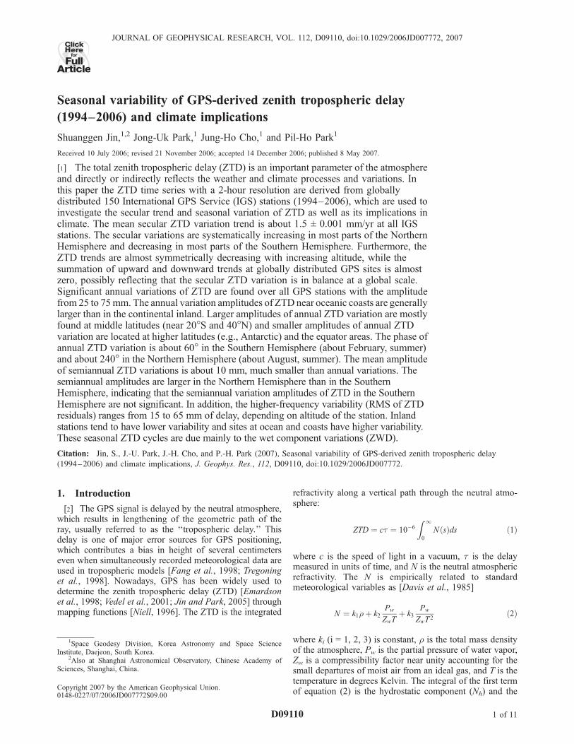
Figure 1. Distribution of global International GPS Service (IGS) GPS sites.

Figure 2. Histogram of the uncertainty for the zenith tro-pospheric delay (ZTD) solutions at 150 sites. Figure 3. Power chart of ZTD time series at Wuhan site.

D09110 JIN ET AL.: SEASONAL VARIABILITY OF ZTD AND CLIMATE IMPLICATIONS

2 of 11

D09110

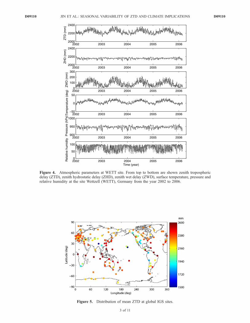
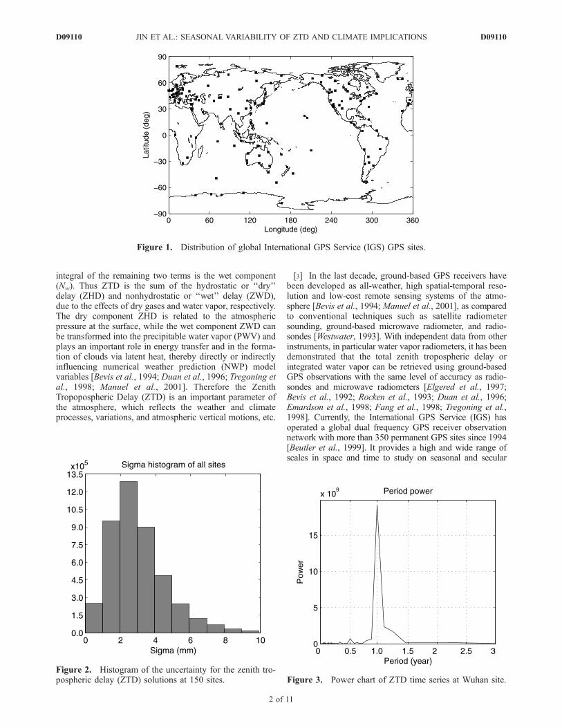
Figure 4. Atmospheric parameters at WETT site. From top to bottom are shown zenith troposphericdelay (ZTD), zenith hydrostatic delay (ZHD), zenith wet delay (ZWD), surface temperature, pressure andrelative humidity at the site Wettzell (WETT), Germany from the year 2002 to 2006.

Figure 5. Distribution of mean ZTD at global IGS sites.


3 of 11

D09110

variations of ZTD as well as its possible implications inclimate.

2. GPS Data and Analysis

2.1. GPS Data

[4] The IGS (International GPS Service) was formallyestablished in 1993 by the International Association ofGeodesy (IAG) and began routine operations on 1 January1994 [Beutler et al., 1999]. The IGS has developed aworldwide network of permanent tracking stations withmore than 350 GPS sites, and each equipped with a GPSreceiver, providing raw GPS orbit and tracking data as adata format called Receiver Independent Exchange (RINEX).Since 1998, the IGS regularly generates a combined tropo-spheric product in the form of weekly files containing thetotal zenith tropospheric delays (ZTD) in 2-hour time intervalfor the IGS tracking stations (ftp://cddis.gsfc.nasa.gov/gps/products/trop_new). However, the IGS did not provide theZTD products before 1998, and furthermore, Humphreys etal. [2004] demonstrated a drastically attenuated oscillation inthe IGS-provided ZTD products between during 1997–2000and 2000–2004, which was probably caused by the com-puted ZTD algorithm and network evolution.[5] Now the fourth Global IGS Data Center in Asian area

was established in 2005 at the Korea Astronomy and SpaceScience Institute (KASI) (http://gdc.kasi.re.kr). It archivesall available near-real-time global IGS observation data(ftp://nfs.kasi.re.kr), including collecting more regional per-manent GPS stations data in Asia-Pacific areas. It willcontribute to geodesy and atmosphere research activitiesin a global scale. This study selects the globally distributed150 IGS sites with better continuous observations spanningmore than 4 years (Figure 1), and most sites observationsare from 1994 to 2006. The long time span of continuousGPS observations provides important information for thelong-term trend and seasonal variation of ZTD.

2.2. Zenith Tropospheric Delay Retrieval Process

[6] The quantity observed by the GPS receiver is theinterferometric phase measurement of the distance from theGPS satellites to the receiver. The processing software mustresolve or model the orbital parameters of the satellites,solve for the transmitter and receiver positions, account for

ionospheric delays, and solve for phase cycle ambiguitiesand the clock drifts, in addition to solving for the tropo-spheric delay parameters of interest. This requires the sametype of GPS data processing software as that which is usedfor high precision geodetic measurements. We use theGAMIT software [King and Bock, 1999], which solves forthe ZTD and other parameters using a constrained batchleast squares inversion procedure. In addition, this studyuses the newly recommended strategies [Byun et al., 2005]to calculate ZTD time series with temporal resolution of2 hours from 1994 to 2006.[7] The GAMIT software parameterizes ZTD as a

stochastic variation from the Saastamoinen model[Saastamoinent, 1973], with piecewise linear interpolationin between solution epochs. GAMIT is very flexible in thatit allows a priori constraints of varying degrees of uncer-tainty. The variation from the hydrostatic delay is con-strained to be a Gauss-Markov process with a specifiedpower density of 2 cm/

ffiffiffiffiffiffiffiffiffihour

p, referred to below as the

‘‘zenith tropospheric parameter constraint.’’ We designed a12-hour sliding window strategy in order to process theshortest data segment possible without degrading the accu-racy of ZTD estimates. The Gauss-Markov process providesan implicit constraint on the ZTD estimate at a given epochfrom observations at proceeding and following epochs,which means that the accuracy is expected to be lower atthe beginning and end of each window. We therefore extractZTD estimates from the middle 4 hours of the window andthen move the window forward by 4 hours. Finally, the ZTDtime series from 1994 to 2006 are obtained at globallydistributed 150 IGS sites with temporal resolution of2 hours. Figure 2 shows the uncertainties for the ZTD solu-tions at 150 sites as a histogram where the vertical axis isthe number of GPS ZTD solutions. It can see that the meanuncertainty of ZTD is about 3 mm.

2.3. Analysis Methods

[8] To fit the time series, a model with a linear trend and aseasonal component for ZTD has been used. This model isdescribed by the following function [Feng et al., 1978]:

ZTDt ¼ aþ bt þX2k¼1

ck sin 2p t � t0ð Þ=pk þ 8kð Þ½ þ et ð3Þ

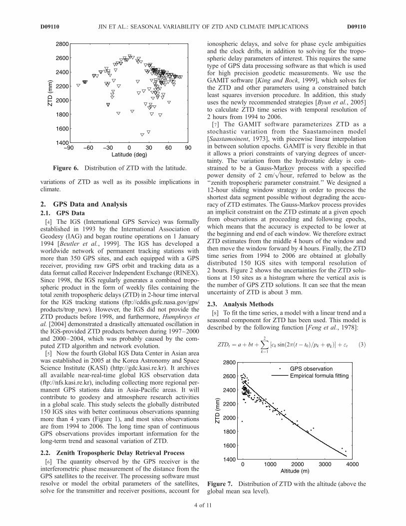
Figure 6. Distribution of ZTD with the latitude.

Figure 7. Distribution of ZTD with the altitude (above theglobal mean sea level).


4 of 11

D09110

where a and b are the constant and linear terms, ck, pk, and8k are the amplitude, period, and phase at period k, respec-tively, and et is the residual. We analyzed all the ZTD timeseries of each GPS station with Fast Fourier transform andfound that the most obvious periods of all GPS stations’ ZTDtime series are about 359.5 days and 180.1 days. Forexample, Figure 3 shows the period power chart of ZTD timeseries at Wuhan (China) GPS site. It has shown clear annualand semiannual variations. No other periods stand out, so wehere analyze the ZTD time series using p1 = 1 year and p2 =0.5 year in equation (3). Through the method of least squareswe can determine the unknown parameters in equation (3) with

the original series of 2-hour ZTD, and then we further analyzethe characteristics of annual and semiannual variations andthose of the constant and linear terms.

3. Results and Discussions

3.1. Zenith Tropospheric Delay

[9] The ZTD consists of the hydrostatic delay (ZHD) andwet delay (ZWD). The ZHD can be well calculated fromsurface meteorological data, ranging from 1.5 to 2.6 m,which accounts for 90% ZTD. It derives from the relation-ship with hydrostatic equilibrium approximation for theatmosphere. Under hydrostatic equilibrium, the change in

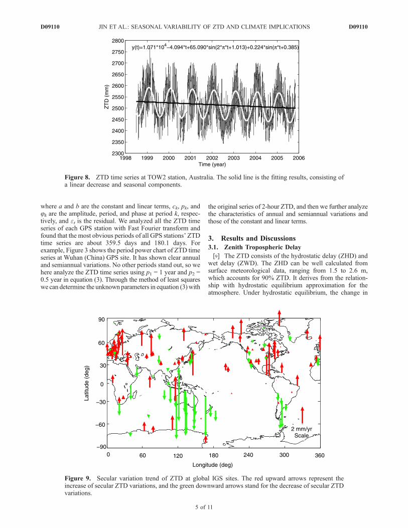
Figure 8. ZTD time series at TOW2 station, Australia. The solid line is the fitting results, consisting ofa linear decrease and seasonal components.

Figure 9. Secular variation trend of ZTD at global IGS sites. The red upward arrows represent theincrease of secular ZTD variations, and the green downward arrows stand for the decrease of secular ZTDvariations.


5 of 11

D09110

pressure with height is related to total density at theheight h above the mean sea level by

dp ¼ �r hð Þg hð Þdh ð4Þ

where r(h)and g(h) are the density and gravity at theheight h. It can be further deduced approximately as

ZHD ¼ kp0 ð5Þ

where k is constant (2.28 mm/hPa) and p0 is the pressure atheight h0 [Davis et al., 1985]. It shows that the ZHD isproportional to the atmospheric pressure at the site. TheZWD is highly variable due possibly to varying climate,relating to the temperature and water vapor. Unfortunately,only fewer IGS sites have meteorological instruments whichcan directly obtain the real ZWD or PWV. If one calculatedthe ZWD or PWV using the meteorological data from theEuropean Centre for Medium-Range Weather Forecasts(ECMWF), it has some differences relative to the realobservation results with meteorological instrument data

[Hagemann et al., 2003]. Therefore we here analyze thevariation and relationship between atmospheric parametersat GPS stations equipped with the meteorological instru-ments. For example, the GPS station Wettzell (WETT),Germany has equipped the meteorological instruments. Thepositions of humidity and temperature sensors are the sameas the GPS antenna, and the pressure sensor is 10.5 m belowthe GPS antenna. The data frequencies of relative humidity,temperature and pressure are all 15 min, and their accuraciesare 1.5% (relative to height), 0.3�C and 0.1 mbar,respectively. Figure 4 shows an example of the time seriesof various atmospheric parameters at the site WETT fromthe year 2002 to 2006. From top to bottom panels, itsequentially denotes zenith tropospheric delay (ZTD),zenith hydrostatic delay (ZHD), zenith wet delay (ZWD),surface temperature, pressure, and relative humidity. Weexamine how much of that correlation between surfacemeasurements. It has been noted that the ZHD is highlyproportional to the atmospheric pressure at the site andrelatively stable, while the ZWD is positively correlatedwith the temperature and also correlated with the relativehumidity. This is due to the combined effects of increasingevaporation and a strong increase in the water vaporsaturation pressure. The correlation coefficient betweenZWD and surface temperature is 0.81, and the remaining ismaybe correlated to the water vapor. The correlationcoefficient between ZTD and ZWD is about 0.95, reflectinga good correlation between ZTD and ZWD variations. Inaddition, we further analyze and compare these parametersat other GPS stations with meteorological data (MATE(Italy), ONSA (Sweden), NYAL (Norway), TSKB (Japan),WES2 (USA), ALGO (USA), FAIR (Alaska, USA), KOKE(Hawaii, USA), and HART (Australia)) and it has shownalmost the same correlations with the WETT station.Therefore it has been indicated that the seasonal variationsof ZTD are due primarily to the wet component (ZWD),even though the wet delay is only 10% of the total delay(ZTD). In addition, the ZHD is proportional to theatmospheric pressure (equation (5)), while the pressure ismainly related to height (seeing the following equation (6)),and therefore the ZHD is almost constant, again showing

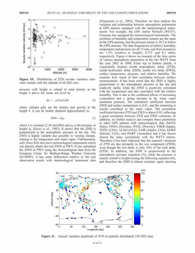
Figure 10. Distribution of ZTD secular variation velo-cities (trend) with the altitude of all IGS sites.

Figure 11. Annual variation amplitude of ZTD at globally distributed 150 GPS sites.


6 of 11

D09110

that the seasonal variations of ZTD are due primarily to theZWD.[10] The mean ZTD values at all GPS sites are shown in

Figure 5 as a color map. It has been noted that lower ZTDvalues are found at the areas of the Tibet (Asia), AndesMountain (South America), Northeast Pacific and higherlatitudes (Antarctica and Arctic), and the higher ZTD valuesare concentrated at the areas of middle-low latitudes (also seeFigure 6). Figure 7 shows the distribution of ZTD at all IGSsites with the altitude (above the global mean sea level). It hasbeen clearly seen that the ZTD values decrease with increas-ing altitude. This is due to the atmospheric pressure variationswith the height increase. Atmospheric pressure is the pressure aboveany area in the Earth’s atmosphere caused by the weight ofair. Air masses are affected by the general atmosphericpressure within the mass, creating areas of high pressure(anticyclones) and low pressure (depressions). Low pressureareas have less atmospheric mass above their locations,whereas high pressure areas have more atmospheric massabove their locations. As elevation increases, there areexponentially fewer and fewer air. Therefore atmosphericpressure decreases with increasing altitude at a decreasingrate. The following relationship is a first-order approximationto the height (http://en.wikipedia.org/wiki/Air_pressure):

log10 P 5� h

15:5ð6Þ

where P is the pressure in Pascals and h is the height inmillimeters. On the basis of equation (5), ZHD can beexpressed as 2.28 * 10(5�h/15.5). As the ZHD accounts for90% of ZTD, we can further deduce the approximate ZTDat all GPS sites as an empirical formula:

ZTD ¼ 2:28 � 10 5�h=15:5ð Þ=0:9 ð7Þ

where the units of ZTD and h are in millimeters,respectively. Comparing GPS-derived ZTD with theempirical formula estimations (Figure 7), it has shown agood consistency.

3.2. Trend Analysis

[11] The GPS ZTD time series have been analyzed for 4–12 years at globally distributed 150 GPS sites. Figure 8 shows

an example of an original ZTD time series and the fittinglines at TOW2 station, Australia. The solid line is the fittingresults, consisting of a linear decrease and seasonal compo-nents (annual and semiannual terms). It has shown a cleartrend and seasonal variations of ZTD time series at theTOW2 in Australia with lower values in the winter andhigher values in the summer. Using the model fromequation (3), the fitting parameters of all GPS site areobtained, including trend and seasonal variation terms. Themean secular ZTD variation trend is about 1.5 ± 0.001 mm/yr.Figure 9 shows the distribution of the secular ZTD variationtrends at all GPS sites as the yearly increase or decrease. Itcan be seen that the trends are positive in most parts of theNorthern Hemisphere and negative in most parts of theSouthern Hemisphere (excluding positive in Antarctic),corresponding to a systematic increase or decrease of ZTD.It is interesting to note that the downtrend in Australia islarger than other regions. This downtrend of ZTD is probablydue to the highly deserted in Australia. In addition, Figure 10shows the relationship of secular ZTD variation trend withthe altitude. It has been seen that the ZTD variation trenddecreases with increasing altitude, and furthermore, the ZTDtrends are almost symmetrical with altitude. This indicatesthat the secular ZTD variations are larger at the lower altitudeand at the higher altitude the secular ZTD variations hardlyincrease or decrease. In addition, the sum of downward andupward trends at globally distributed GPS sites is almostzero, which possibly indicates that the secular variation is inbalance at a global scale, but subjecting to unevenly distrib-uted GPS stations, etc. It need further be confirmed withmuch denser GPS network in the future. These secular ZTDvariation characteristics reflect the total variations of surfaceatmospheric pressure, temperature and relative humidity,atmospheric vertical motions, etc.

3.3. Seasonal Cycle

[12] Meanwhile, the seasonal components are alsoobtained using equation (3), which can be used to studythe seasonal cycle, including amplitude and phase shift. Thefitted phase shift is used to determine in which month theseasonal maximum takes place. The annual variation of ZTDranges from 25 to 75 mm depending on the site, and the

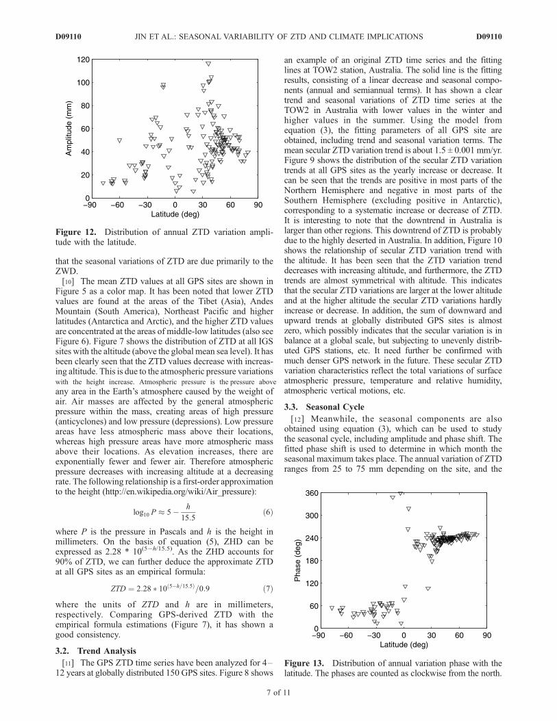
Figure 12. Distribution of annual ZTD variation ampli-tude with the latitude.

Figure 13. Distribution of annual variation phase with thelatitude. The phases are counted as clockwise from the north.


7 of 11

D09110

average amplitude is about 50 mm at most sites (Figure 11).The annual variation amplitudes of ZTD at the IGS sites nearoceanic coasts are generally larger than in the continentalinland. In addition, larger amplitudes of annual ZTD varia-tion are mostly found at middle-low latitudes (near 20�S and40�N), and the amplitudes of annual ZTD variation areespecially smaller at higher latitudes (e.g., Antarctic andArctic) and the equator areas (see Figure 12). Sites on theeastern Atlantic and northeast Pacific coasts have lowerannual variations, probably because of the moderating effectof the ocean on climate. Sites on the lee side of the Alps havehigher annual variation, possibly due to the combined effectsof a rain shadow in the winter and high moisture from theMediterranean in the summer [Haase et al., 2001, 2003;Deblonde et al., 2005]. Figure 13 shows the annual phasedistribution with the latitude, where phase values are countedas clockwise from the north. It can be seen that the phase ofannual ZTD variation is almost found at about 60� (aboutFebruary, summer) in the Southern Hemisphere and at about240� (about August, summer) in the Northern Hemisphere,which is just a half-year difference.[13] The semiannual variations of ZTD at globally dis-

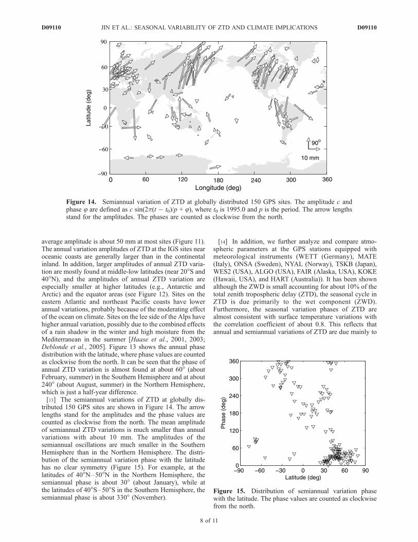
tributed 150 GPS sites are shown in Figure 14. The arrowlengths stand for the amplitudes and the phase values arecounted as clockwise from the north. The mean amplitudeof semiannual ZTD variations is much smaller than annualvariations with about 10 mm. The amplitudes of thesemiannual oscillations are much smaller in the SouthernHemisphere than in the Northern Hemisphere. The distri-bution of the semiannual variation phase with the latitudehas no clear symmetry (Figure 15). For example, at thelatitudes of 40�N–50�N in the Northern Hemisphere, thesemiannual phase is about 30� (about January), while atthe latitudes of 40�S–50�S in the Southern Hemisphere, thesemiannual phase is about 330� (November).

[14] In addition, we further analyze and compare atmo-spheric parameters at the GPS stations equipped withmeteorological instruments (WETT (Germany), MATE(Italy), ONSA (Sweden), NYAL (Norway), TSKB (Japan),WES2 (USA), ALGO (USA), FAIR (Alaska, USA), KOKE(Hawaii, USA), and HART (Australia)). It has been shownalthough the ZWD is small accounting for about 10% of thetotal zenith tropospheric delay (ZTD), the seasonal cycle inZTD is due primarily to the wet component (ZWD).Furthermore, the seasonal variation phases of ZTD arealmost consistent with surface temperature variations withthe correlation coefficient of about 0.8. This reflects thatannual and semiannual variations of ZTD are due mainly to

Figure 14. Semiannual variation of ZTD at globally distributed 150 GPS sites. The amplitude c andphase 8 are defined as c sin(2p(t � t0)/p + 8), where t0 is 1995.0 and p is the period. The arrow lengthsstand for the amplitudes. The phases are counted as clockwise from the north.

Figure 15. Distribution of semiannual variation phasewith the latitude. The phase values are counted as clockwisefrom the north.


8 of 11

D09110

the ZWD variations, about 80% in the surface temperatureand 20% mainly in water vapor variations.

3.4. High-Frequency ZTD Variations

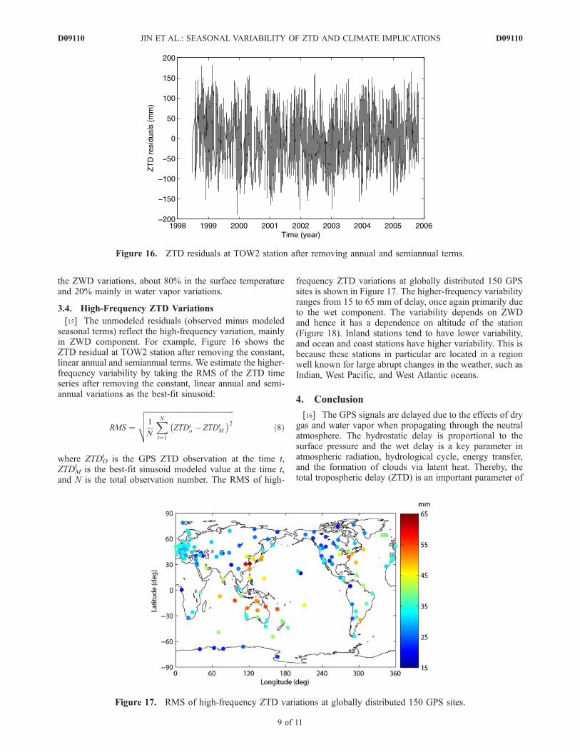
[15] The unmodeled residuals (observed minus modeledseasonal terms) reflect the high-frequency variation, mainlyin ZWD component. For example, Figure 16 shows theZTD residual at TOW2 station after removing the constant,linear annual and semiannual terms. We estimate the higher-frequency variability by taking the RMS of the ZTD timeseries after removing the constant, linear annual and semi-annual variations as the best-fit sinusoid:

RMS ¼

ffiffiffiffiffiffiffiffiffiffiffiffiffiffiffiffiffiffiffiffiffiffiffiffiffiffiffiffiffiffiffiffiffiffiffiffiffiffiffiffiffiffiffiffiffiffiffiffiffi1

N

XNt¼1

ZTDto � ZTDt

M

� �2vuut ð8Þ

where ZTDOt is the GPS ZTD observation at the time t,

ZTDMt is the best-fit sinusoid modeled value at the time t,

and N is the total observation number. The RMS of high-

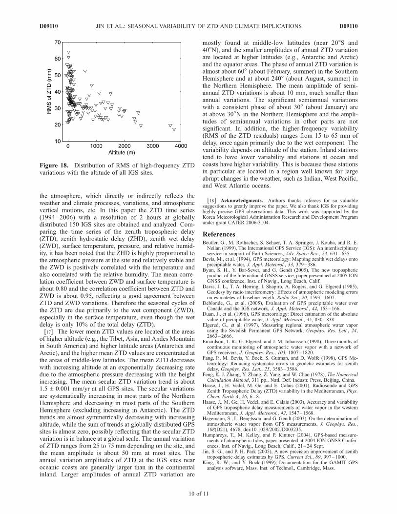
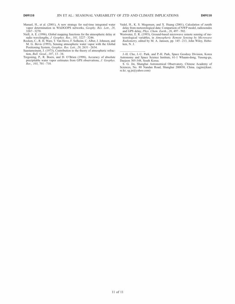
frequency ZTD variations at globally distributed 150 GPSsites is shown in Figure 17. The higher-frequency variabilityranges from 15 to 65 mm of delay, once again primarily dueto the wet component. The variability depends on ZWDand hence it has a dependence on altitude of the station(Figure 18). Inland stations tend to have lower variability,and ocean and coast stations have higher variability. This isbecause these stations in particular are located in a regionwell known for large abrupt changes in the weather, such asIndian, West Pacific, and West Atlantic oceans.

4. Conclusion

[16] The GPS signals are delayed due to the effects of drygas and water vapor when propagating through the neutralatmosphere. The hydrostatic delay is proportional to thesurface pressure and the wet delay is a key parameter inatmospheric radiation, hydrological cycle, energy transfer,and the formation of clouds via latent heat. Thereby, thetotal tropospheric delay (ZTD) is an important parameter of

Figure 16. ZTD residuals at TOW2 station after removing annual and semiannual terms.

Figure 17. RMS of high-frequency ZTD variations at globally distributed 150 GPS sites.


9 of 11

D09110

the atmosphere, which directly or indirectly reflects theweather and climate processes, variations, and atmosphericvertical motions, etc. In this paper the ZTD time series(1994–2006) with a resolution of 2 hours at globallydistributed 150 IGS sites are obtained and analyzed. Com-paring the time series of the zenith tropospheric delay(ZTD), zenith hydrostatic delay (ZHD), zenith wet delay(ZWD), surface temperature, pressure, and relative humid-ity, it has been noted that the ZHD is highly proportional tothe atmospheric pressure at the site and relatively stable andthe ZWD is positively correlated with the temperature andalso correlated with the relative humidity. The mean corre-lation coefficient between ZWD and surface temperature isabout 0.80 and the correlation coefficient between ZTD andZWD is about 0.95, reflecting a good agreement betweenZTD and ZWD variations. Therefore the seasonal cycles ofthe ZTD are due primarily to the wet component (ZWD),especially in the surface temperature, even though the wetdelay is only 10% of the total delay (ZTD).[17] The lower mean ZTD values are located at the areas

of higher altitude (e.g., the Tibet, Asia, and Andes Mountainin South America) and higher latitude areas (Antarctica andArctic), and the higher mean ZTD values are concentrated atthe areas of middle-low latitudes. The mean ZTD decreaseswith increasing altitude at an exponentially decreasing ratedue to the atmospheric pressure decreasing with the heightincreasing. The mean secular ZTD variation trend is about1.5 ± 0.001 mm/yr at all GPS sites. The secular variationsare systematically increasing in most parts of the NorthernHemisphere and decreasing in most parts of the SouthernHemisphere (excluding increasing in Antarctic). The ZTDtrends are almost symmetrically decreasing with increasingaltitude, while the sum of trends at globally distributed GPSsites is almost zero, possibly reflecting that the secular ZTDvariation is in balance at a global scale. The annual variationof ZTD ranges from 25 to 75 mm depending on the site, andthe mean amplitude is about 50 mm at most sites. Theannual variation amplitudes of ZTD at the IGS sites nearoceanic coasts are generally larger than in the continentalinland. Larger amplitudes of annual ZTD variation are

mostly found at middle-low latitudes (near 20�S and40�N), and the smaller amplitudes of annual ZTD variationare located at higher latitudes (e.g., Antarctic and Arctic)and the equator areas. The phase of annual ZTD variation isalmost about 60� (about February, summer) in the SouthernHemisphere and at about 240� (about August, summer) inthe Northern Hemisphere. The mean amplitude of semi-annual ZTD variations is about 10 mm, much smaller thanannual variations. The significant semiannual variationswith a consistent phase of about 30� (about January) areat above 30�N in the Northern Hemisphere and the ampli-tudes of semiannual variations in other parts are notsignificant. In addition, the higher-frequency variability(RMS of the ZTD residuals) ranges from 15 to 65 mm ofdelay, once again primarily due to the wet component. Thevariability depends on altitude of the station. Inland stationstend to have lower variability and stations at ocean andcoasts have higher variability. This is because these stationsin particular are located in a region well known for largeabrupt changes in the weather, such as Indian, West Pacific,and West Atlantic oceans.

[18] Acknowledgments. Authors thanks referees for so valuablesuggestions to greatly improve the paper. We also thank IGS for providinghighly precise GPS observations data. This work was supported by theKorea Meteorological Administration Research and Development Programunder grant CATER 2006-3104.

ReferencesBeutler, G., M. Rothacher, S. Schaer, T. A. Springer, J. Kouba, and R. E.Neilan (1999), The International GPS Service (IGS): An interdisciplinaryservice in support of Earth Sciences, Adv. Space Res., 23, 631–635.

Bevis, M., et al. (1994), GPS meteorology: Mapping zenith wet delays ontoprecipitable water, J. Appl. Meteorol., 33, 379–386.

Byun, S. H., Y. Bar-Sever, and G. Gendt (2005), The new troposphericproduct of the International GNSS service, paper presentaed at 2005 IONGNSS conference, Inst. of Navig., Long Beach, Calif.

Davis, J. L., T. A. Herring, I. Shapiro, A. Rogers, and G. Elgered (1985),Geodesy by radio interferometry: Effects of atmospheric modeling errorson esimatetes of baseline length, Radio Sci., 20, 1593–1607.

Deblonde, G., et al. (2005), Evaluation of GPS precipitable water overCanada and the IGS network, J. Appl. Meteorol., 44, 153–166.

Duan, J., et al. (1996), GPS meteorology: Direct estimation of the absolutevalue of precipitable water, J. Appl. Meteorol., 35, 830–838.

Elgered, G., et al. (1997), Measuring regional atmospheric water vaporusing the Swedish Permanent GPS Network, Geophys. Res. Lett., 24,2663–2666.

Emardson, T. R., G. Elgered, and J. M. Johansson (1998), Three months ofcontinuous monitoring of atmospheric water vapor with a network ofGPS receivers, J. Geophys. Res., 103, 1807–1820.

Fang, P., M. Bevis, Y. Bock, S. Gutman, and D. Wolfe (1998), GPS Me-teorology: Reducing systematic errors in geodetic estimates for zenithdelay, Geophys. Res. Lett., 25, 3583–3586.

Feng, K, J. Zhang, Y. Zhang, Z. Yang, and W. Chao (1978), The NumericalCalculation Method, 311 pp., Natl. Def. Industr. Press, Beijing, China.

Haase, J., H. Vedel, M. Ge, and E. Calais (2001), Radiosonde and GPSZenith Tropospheric Delay (ZTD) variability in the Mediterranean, Phys.Chem. Earth A, 26, 6–8.

Haase, J., M. Ge, H. Vedel, and E. Calais (2003), Accuracy and variabilityof GPS tropospheric delay measurements of water vapor in the westernMediterranean, J. Appl. Meteorol., 42, 1547–1568.

Hagemann, S., L. Bengtsson, and G. Gendt (2003), On the determination ofatmospheric water vapor from GPS measurements, J. Geophys. Res.,108(D21), 4678, doi:10.1029/2002JD003235.

Humphreys, T., M. Kelley, and P. Kintner (2004), GPS-based measure-ments of atmospheric tides, paper presented at 2004 ION GNSS Confer-ences, Inst. of Navig., Long Beach, Calif., 21–24 Sept.

Jin, S. G., and P. H. Park (2005), A new precision improvement of zenithtropospheric delay estimates by GPS, Current Sci., 89, 997–1000.

King, R. W., and Y. Bock (1999), Documentation for the GAMIT GPSanalysis software, Mass. Inst. of Technol., Cambridge, Mass.

Figure 18. Distribution of RMS of high-frequency ZTDvariations with the altitude of all IGS sites.


10 of 11

D09110

Manuel, H., et al. (2001), A new strategy for real-time integrated watervapor determination in WADGOPS networks, Geophy. Res. Lett., 28,3267–3270.

Niell, A. E. (1996), Global mapping functions for the atmospheric delay atradio wavelengths, J. Geophys. Res., 101, 3227–3246.

Rocken, C., R. H. Ware, T. Van Hove, F. Solheim, C. Alber, J. Johnson, andM. G. Bevis (1993), Sensing atmospheric water vapor with the GlobalPositioning System, Geophys. Res. Lett., 20, 2631–2634.

Saastamoinent, J. (1973), Contribution to the theory of atmospheric refrac-tion, Bull. Geod., 107, 13–34.

Tregoning, P., R. Boers, and D. O’Brien (1998), Accuracy of absoluteprecipitable water vapor estimates from GPS observations, J. Geophys.Res., 103, 701–710.

Vedel, H., K. S. Mogensen, and X. Huang (2001), Calculation of zenithdelay from meteorological data: Comparison of NWP model, radiosondesand GPS delay, Phys. Chem. Earth., 26, 497–502.

Westwater, E. R. (1993), Ground-based microwave remote sensing of me-teorological variables, in Atmospheric Remote Sensing by MicrowaveRadiometry, edited by M. A. Janssen, pp. 145–213, John Wiley, Hobo-ken, N. J.

��J.-H. Cho, J.-U. Park, and P.-H. Park, Space Geodesy Division, Korea

Astronomy and Space Science Institute, 61-1 Whaam-dong, Yusong-gu,Daejeon 305-348, South Korea.S. G. Jin, Shanghai Astronomical Observatory, Chinese Academy of

Sciences, No. 80 Nandan Road, Shanghai 200030, China. ([email protected]; [email protected])


11 of 11

D09110

Seasonal variability of GPS-derived Zenith Tropospheric Delay (1994-2006) and climate implications

Documents

Transcript of Seasonal variability of GPS-derived Zenith Tropospheric Delay (1994-2006) and climate implications