Finite Prandtl Number 2-D Convection at High Rayleigh Number

Finite Prandtl Number 2-D Convection at HighRayleigh Number

Catherine Hier Majumder1,2, David A. Yuen1,2, Erik O. Sevre1,2, John M. Boggs2,and Stephen Y. Bergeron2

1. Department of Geology and Geophysics, University of Minnesota, Minneapolis, MN 2. Minnesota Supercomputer Institute, University of Minnesota, Minneapolis, MN

submitted to Electronic Geosciences http://www.msi.umn.edu/~cathy/prpaper/paper.html

Abstract

Finite Prandtl number thermal convection is important to the dynamics of planetarybodies in the solar system. For example, the complex geology on the surface of theJovian moon Europa is caused by a convecting, brine-rich global ocean that deforms theoverlying icy "lithosphere". We have conducted a systematic study on the variations of the convection style, as Prandtl numbers are varied from 7 to 100 at Rayleigh numbers

106 and 108. Numerical simulations show that changes in the Prandtl number could exertsignificant effects on the shear flow, the number of convection cells, the degree oflayering in the convection, and the number and size of the plumes in the convectingfluid. We found that for a given Rayleigh number, the convection style can change fromsingle cell to layered convection, for increasing Prandtl number from 7 to 100. Theseresults are important for determining the surface deformation on the Jovian moonEuropa. They also have important implications for surface heat flow on Europa, or forthe interior heat transfer of the early Earth during its magma ocean phase.

Introduction

The Prandtl number is the ratio of the kinematic viscosity to the thermal diffusivity of afluid and is an important control variable in thermal convection. Although infinitePrandtl number approximations are appropriate for the Earth’s crust and mantle, finitePrandtl number fluids are also ubiquitous throughout our Earth. They include many ofthe fluids associated with our everyday lives, such as air, water, alcohols, and oils. Convection in air, which has a Prandtl number of about 1, is responsible for the weather. Convection in water, with a Prandtl number of 7, is important for oceanic currents. Theliquid iron of the Earth’s outer core is a finite Prandtl fluid. Convection in thiselectrically conducting fluid generates the Earth’s magnetic field (Glatzmaier andRoberts, 1995) . Finite Prandtl convection is important to crystallization processes in

magma chambers (Bergantz, 1992). Convection in a magma ocean under high Rayleighand Prandtl number conditions was likely to have occurred early in Earth’s history.

A knowledge of convection styles in this type of fluid may give important insights intothe heat flux and chemical differentiation of the early Earth. Finite Prandtl number flowsare especially important to the dynamics of the outer planets and their moons. Thesurface of Jupiter is formed by convection in a fluid with a Prandtl number of around0.01 (Zhang and Schubert, 2000). The Galileo missions have confirmed the existence ofconvecting oceans on the Jovian moons Europa and Callisto (Carr, 1998, Khurana,1998). Thomas and Delaney (2001) have used numerical models to show that a sea-floorspreading and hydrothermal vent system similar to the Earth’s mid-ocean ridges couldproduce convection in Europa’s global ocean. A magnetic field is induced as the salty,convecting, global oceans on the moons Europa and Callisto are dragged throughJupiter’s magnetosphere (Khurana, 1998). Europa’s icy lithosphere has a wealth ofsurface geology created by convection in its global ocean (Carr et al., 1998). Evidencefrom the Voyager missions indicates that the surface features of Ganymede may be due toconvection in a water-ice mantle, which is overlain by an icy lithosphere (Kirk, 1987). Abetter understanding of finite Prandtl number convection at high Rayleigh numbers willallow us to better model heat flux and surface deformation on the Jovian moons.

Numerical simulations of Rayleigh-Bénard convection at both high Rayleigh and Prandtlnumber are difficult. As the Rayleigh number increases, strong inertial forces generatecomplex structures in the temperature and velocity fields that require increased gridpoints and smaller timesteps. Increasing the Prandtl number leads to sharp temperaturegradients and strong shear flows. These effects also require increasing grid points anddecreasing timesteps. The problem is compounded by the fact that as the Prandtl numberis increased the fluid becomes stiffer and more time is required for movement to developfrom an initial temperature and velocity perturbation. Vincent and Yuen (1999, 2000)have conducted numerical simulations for a Prandtl number of unity (air) at Rayleighnumbers from 108 to 1014. Numerical simulations have been conducted for Prandtlnumber 7 (water) up to Rayleigh numbers of 1013 (Yuen et al., 2000). These simulationsshowed the complex structures generated by finite Prandtl convection, and wavelets to bean ideal tool for understanding the multiscale nature of these structures (Yuen et al.,2000).

Heat flux scaling laws tend to show that the Nusselt number is proportional to (RaPr)n

where n is 1/3 for plume theories with a single length scale and 2/7 for plume theorieswith several length scales (Zaleski, 2000). Grossmann and Lohse (2000) suggest that asingle power law may not appropriately explain the dependence of the Nusselt number onthe Rayleigh and Prandtl numbers since more than one heat transport regime may be

operating in a given experiment. Instead they propose that linear combinations of severalpower laws may be necessary. They also indicate that for Pr > 7 formation of the windof turbulence, on which classic scaling theories are based becomes less likely. The windof turbulence is associated with shearing in the boundary layers that moves plumes in thehorizontal direction and results in a bulk stirring of the fluid. Verzicco and Camussi(1999) conducted numerical experiments for Prandtl numbers ranging from 0.022(mercury) to 15 at Rayleigh number 6 x 105. They found that below Pr = 0.35 heat istransferred by large-scale recirculation cells; above Pr = 0.35 the heat is transferred bythermal plumes. The aspect-ratio (A) may also play an important role in the heattransport, as suggested by the Shraiman and Siggia (1990) theory, in which the Nusseltnumber is predicted to be proportional to Ra2/7Pr-1/7A-3/7.

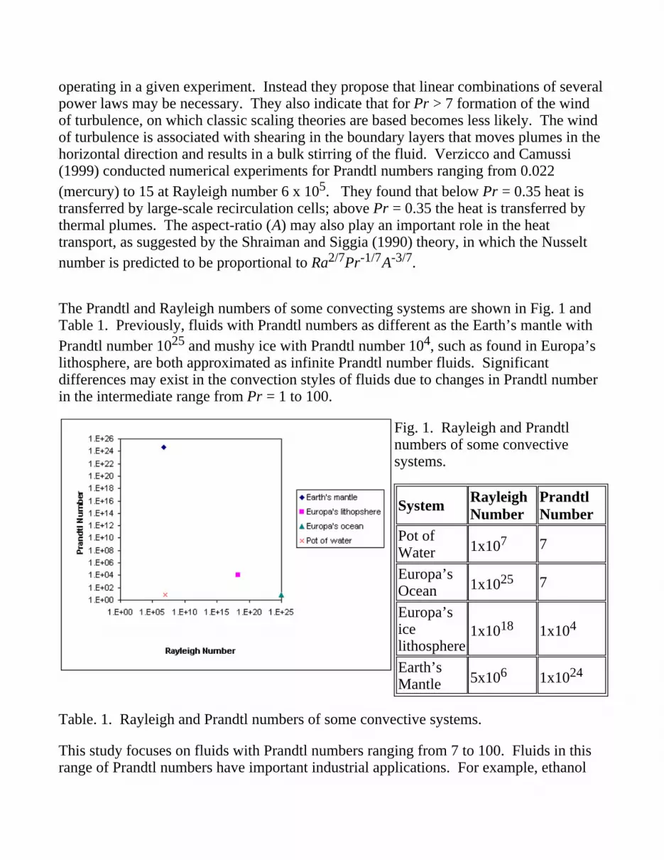
The Prandtl and Rayleigh numbers of some convecting systems are shown in Fig. 1 andTable 1. Previously, fluids with Prandtl numbers as different as the Earth’s mantle withPrandtl number 1025 and mushy ice with Prandtl number 104, such as found in Europa’slithosphere, are both approximated as infinite Prandtl number fluids. Significantdifferences may exist in the convection styles of fluids due to changes in Prandtl numberin the intermediate range from Pr = 1 to 100.

Fig. 1. Rayleigh and Prandtlnumbers of some convectivesystems.

System RayleighNumber

PrandtlNumber

Pot ofWater 1x107 7

Europa’sOcean 1x1025 7

Europa’sicelithosphere

1x1018 1x104

Earth’sMantle 5x106 1x1024

Table. 1. Rayleigh and Prandtl numbers of some convective systems.

This study focuses on fluids with Prandtl numbers ranging from 7 to 100. Fluids in thisrange of Prandtl numbers have important industrial applications. For example, ethanol

has a Prandtl number of 17. A solution of 60% glycerin and 40% water has a Prandtlnumber of 100. Shevtsova et al. studied the onset of thermocapillary convection in liquidbridges for fluids with Prandtl numbers up to 35. This type of convection can causeundesired compositional variations in crystals grown industrially.

We simulated convection at Rayleigh numbers of 106 and 108. The Prandtl numbers inthis study are still significantly below those of some important geologic fluids such as themushy ice that forms diapirs on Europa, or basaltic magma. Both of these fluids havePrandtl numbers of order 104. This study represents a first step in the process ofsimulating systems such as Europa. It allows us to begin to asses the importance ofPrandtl number in the behavior of Rayleigh-Bénard convection at higher Prandtlnumbers. It represents the beginning of the development of techniques that will allow usto conduct simulations at even higher Prandtl and Rayleigh numbers in the future.

We have conducted simulations in an aspect-ratio 3 box for Prandtl numbers of 7, 17, 40,80, and 100 at a Rayleigh number of 106 and for Prandtl numbers of 7, 17, 40, 60, 80, and100 at a Rayleigh number of 108. The convection simulations have a complex timeevolution, which is discussed in detail for the simulations of Prandtl number 7 andRayleigh number 106. We have illustrated the time evolution through the use ofanimations. We have conducted wavelet analysis on the long-term solutions of thetemperature deviation and vorticity fields for each of the simulations to help characterizethe convection style.

Wavelets have been used as a tool to better understand the convection patterns capturedby seismic tomography of the Earth’s mantle (Bergeron et al., 1999, 2000, Yuen et al.,2000). One dimensional wavelet transforms have been used for many years in theanalysis of time series, such as the interseasonal Earth rotation variations (Chao andNaito, 1995). Malamud and Turcotte (2001) analyzed one-dimensional tracks of Martiantopography using wavelets. Vecsey and Matyska (2001) used wavelets to analysistemperature, kinetic energy, and Nusselt number time series in mantle convectionsimulations. Castillo et al. (2001) used wavelet transforms of seismograms tocharacterize the transition zone structure below California.

Wavelets are also a powerful tool for processing 2-D convection simulation data, such astemperature and vorticity fields (Hier et al., 2000). Temperature and vorticity maps fromconvection simulations can be quite complicated and difficult to interpret at higherRayleigh and Prandtl numbers. The wavelet transform allows us to separate thelarge-scale features, such as convection cells, from smaller scale features, such as shearlayers. This leads to a better understanding of the different processes that produce thetemperature and vorticity maps.

In order to take advantage of the web format for paper publishing, we have used figuresextensively in this paper. We focus on the temperature deviation and vorticity fieldsgenerated by the simulations along with their wavelet transforms. The finite Prandtlsimulations resulted in rich patterns in the temperature deviation and vorticity fields thatis most easily conveyed by figures. The time evolution of the simulations was also veryrich. The web format has allowed us to feature in this communication animations of howthe complex dynamics develop with time.

Numerical Model

The nondimensional equations of finite Prandtl number convection in the Boussinesqapproximation are:(1)

(2)

(3)

where t is the time nondimensionalized by the thermal diffusivity, T is the temperaturedeviation from the conductive profile, V is the velocity vector, P is the pressure, and ez is

the unit vector from the top to the bottom of the fluid layer. Ra is the Rayleigh numberfor Rayleigh-Bénard convection in a basely heated box, and Pr is the Prandtl number.

The numerical method used is a spectral method for 2-D convection with finite Prandtlnumber (Vincent and Yuen, 1999) with sine and cosine series expansion as the basisfunctions. The top and bottom of the box have free-slip boundary conditions. Thetime-marching uses a mixed leap frog-Cranck-Nicholson two-step pressure correctionscheme. The grid size for each simulation is shown in Table 2. The aspect-ratio of thebox is defined as the width of the box over the layer depth.

Rayleigh Number Prandtl Number Aspect-Ratio (width x depth)

Grid Size (width x depth)

106 7 3 x 1 768x256 points

106 17 3 x 1 768x256 points

106 40 3 x 1 768x256 points

106 80 3 x 1 768x256 points

106 100 3 x 1 1080x360 points

108 7 3 x 1 1080x360 points

108 17 3 x 1 1080x360 points

108 40 3 x 1 1080x360 points

108 60 3 x 1 1080x360 points

108 80 3 x 1 1080x360 points

108 100 3 x 1 1080x360 points

Table 2. Grid size for simulations.

Wavelet Transform

Wavelet transform (e.g. Resnikoff and Weiss, 1998) allows one to study the scales withina dataset without losing the spatial information. Whereas the Fourier transform orspherical harmonics provides a global description of a wavelength over a dataset; thewavelet transform provides a localized description of a particular length scale at each gridpoint in the multidimensional dataset (van den Berg, 1999). The 2-D wavelet transformis:

(4)

where vector b is the two-dimensional position parameter, scalar a is the scalingparameter, and Lx and Ly are the lengths of the periodic rectangle in Cartesian space(Bergeron et al., 2000). We have used as the mother wavelet the Mexican Hat, or thesecond-derivative of the Gaussian function (Daubechies, 1992):

(5)

The wavelet transform is done in Fourier space to simplify and speed-up the calculation(Bergeron et al., 2000).

Scalogram

The result of a Fourier transform is a coefficient describing the strength of a givenwavelength over the whole dataset. The spatial or phase information is not explicitlypreserved. Therefore, you cannot compare the strength of a given wavelength at twodifferent points.

The wavelet transform produces a coefficient describing the strength of a given lengthscale at each data point. The wavelet transform of a 2-D dataset is a 3-D function knownas a scalogram. The scalogram is a function of both the position vector and the scale. The spatial information is explicitly preserved in the scalogram. This allows one toanalyze how the length scale varies with position. One can say that large length scalesare more important at point a, and small length scales are more important at point b.

Since a scalogram is a function of both scale and position, the dimension of the originaldataset is increased by one. Scalograms of our two-dimensional vorticity fields arethree-dimensional boxes. The extra dimensionality makes the scalograms difficult tostore and visualize because of the large memory required. The 3-D boxes contain vastamounts of data that cannot be easily digested by the eye when displayed on a computerscreen. Therefore, we took slices of the box at a given scale. For each scalogram we took3 slices: one at a large-scale, one at a medium-scale, and one at a small-scale. Theseindividual slices are a function of position only. They show the importance of features ata given scale at different positions in space (Fig. 12).

E-max and k-max

The scale parameter in the wavelet transform (Eq. 4) results in a dimensionality of onedegree higher than the physical space analyzed. This can make the scalograms difficultto visualize and interpret. Analysis of E-max and k-max distributions is used tosynthesize the scalogram (Bergeron et al., 2000, Yuen et al., 2000). E-max represents theenergy of the scale that has the largest energy value at a given position. An E-max mapplots the energy value of the scale with the highest energy at a given point in space. It,

therefore, selects the energy value from the scale which is most important at that point.We define the energy of the wavelet transform as the L2-norm:

(6)

Since the sign of both the thermal anomaly and the vorticity is important in convectionstudies, we have multiplied the L2-norm by the original sign of the thermal anomaly or

vorticity function.

The k-max is the wavenumber at which maximum energy occurs for a given positionvector b. A k-max map plots the scale that is most important at a given point. The scale,a, is related to the wavenumber, k, by:

(7)

where ß is a tuning parameter, which we have chosen as 0.22. High k-max valuesrepresent small-scale features. These features are associated with areas of stronggradients. Therefore, the k-max map is an excellent tool for picking out areas of stronggradients in a dataset. For temperature deviation and vorticity fields from convectionsimulations, the areas of sharp gradients are associated with fluid movement. We willuse the k-max maps to emphasize areas of relative movement within the fluid.

The E-max and k-max analysis results in a lower dimensional approximation of the data. It allows us to look at the data over a given range of scales. For example, to studysmall-scale features in the dataset we would find E-max and k-max maps for scalesvarying from k = 15 to k = 20.

Temporal Evolution

The temporal evolution of the simulations is best illustrated by an animation. Animation1 shows the temporal evolution for the Ra = 106 and Pr = 7 simulation. An example ofa fluid with Pr = 7 is water at 20oC and 1 atm (Weast, 1987). The animation shows thetemperature deviation, which is the total temperature minus the conductive profile, andthe vorticity.

Animation 1. Temporal Evolution of Ra = 106 and Pr = 7 simulation for an aspect-ratio of 3.

Click on picture below to start animation.

The simulations are begun from an initial temperature deviation and vorticityperturbations in the form of a sine wave with fundamental wavelength Lx/2 (Fig. 2). Thenumber of gridpoints for the simulation is specified in Table 2.

Fig. 2. The dimensionless time, t =0.000 for Ra = 106, Pr = 7.

For Ra = 106 and Pr = 7, plumes and circulation cells develop from these perturbations.

The plumes have thin stems with thicker plumeheads that spread horizontally along thethermal boundary layers (Fig. 3). The vorticity shows that the circulation cells havepronounced shear layers along the edges with relatively weak rotation in their cores (Fig.3). This indicates that the majority of the movement is along the edge of the convectioncells. Hot material rises vertically in plumes along on edge of a convection cell, and coldmaterial descends vertically in downwellings along the opposite edge. There is onlyweak movement in the central area of the circulation cell.


As the Ra = 106, Pr = 7 simulation advances to t = 0.410, the plumeheads spreadhorizontally across the thermal boundary layer and begin to impinge on neighboringplumeheads, they move down forming regions of hot material below the upper thermalboundary layer (Fig. 4). This creates a new thermal boundary layer. New plumes beginto develop from the original stem region below the hot regions. In the vorticity field thecenter of the circulation cells reverse flow directions (Fig. 4). The sharp shear layersalong the edges of the circulation cells remain in the same orientation as in Fig. 3. Theseshear layers are associated with the new plumes arising from the original stem area.

Fig. 4. The dimensionless time, t =0.410 for Ra = 106, Pr=7.

In the next frame of the temperature deviation we can see new plumes and downwellingsoriginating from the new central thermal boundary layers (Fig. 5). The verticalsymmetry, which originates from the symmetrical initial condition, is still maintained. The plumes and downwellings growing from the original lower thermal boundary layerbegin to form caps below the lower thermal boundary layer. The original vorticity cellsbegin to divide, thus forming two separate layers of circulation cells. This results inlayered convection (Fig. 5).


At time t = 0.420, the plumes growing from the center become connected with thosegrowing from the bottom of the box to form a branched plume structure (Fig. 6). Newplumes develop at the junction of this branch.


At t = 0.430, the layering structure still persists. The plume branching results in avorticity pattern that is a combination of a whole box circulation with a layered structure(Fig. 7). We can still see the original four circulation cells that cover the whole height ofthe box. These four cells are now each divided into three separate layers with thestrongest circulation in the middle layer.


At t = 0.473, the layered circulation cells divide to form vortex pairs (Fig. 8). Smallplumes begin to rise from both the lower and middle thermal boundary layers, anddownwellings form at both the upper and middle thermal boundary layers. The newplumes and downwellings are evenly spaced along the length of the boundary layers. The symmetry originating from the initial condition is preserved.


As convection progresses to t = 0.490, however, the layering that has developeddisappears (Fig. 9). As can be seen in the vorticity field, the four original circulationcells are no longer divided horizontally (Fig. 9). Instead they are each divided verticallyinto three long narrow cells. At t = 0.490, the symmetry which had been carried alongfrom the initial condition is lost.


At t = 0.525, the layered mode is destroyed, and the circulation cells take up the wholebox height (Fig. 10). Although the four circulation cells are still visible, the circulation isreversed from that of the original cells. There is a strong horizontal shear componentresulting in a wind that sweeps across the box. The temperature deviation shows that theplumes move up from the lower thermal boundary layer along thin stems, which are tiltedby the horizontal shear (Fig. 10). The plumes and downwellings spread out horizontallyonce they reach the top and bottom with relatively thick thermal boundary layers.


The long-term solution is reached at t = 0.534. In the long-term solution there are stillfour convection cells, but two of the cells have become wider at the expense of two cellswhich have narrowed (Fig. 11). The horizontal shear remains in the long-term solution. This results in shear layers on the edge of the wide convection cells.

Fig. 11. Long-term solution, at thedimensionless time, t = 0.534 for Ra = 106, Pr = 7.

Wavelet Analysis

The use of wavelets allows us to separate the structures seen in the temperature deviationand vorticity datasets by the scale of the features. This helps us to interpret the processesoperating at different scales in the convection pattern. The long-term solution of thetemperature deviation and vorticity fields for each simulations was transformed using thecontinuous wavelet transform (Eq. 4) with the Mexican Hat as the mother wavelet (Eq.5). The scalogram was computed from local wavenumber k = 1 to k = 20, whichcorresponds to a resolution varying from 65 to 1.2% of the horizontal box width. Theresulting scalogram for Ra = 106 and Pr = 7 is a 16 MB file, which consists of a 3-Dbox with 768 x 256 x 20 points. The scalogram is difficult to visualize due to the largememory required and to the fact that it contains more information then can be easilydigested by the eye. Therefore, for better interpretation and to minimize data storage, wehave taken slices of the scalogram at 3 scales: k = 5, k =11, and k = 20, whichcorresponds to resolutions of 27, 7.3, and 1.2% of the box width (Fig. 12 & 13).

For the simulation Ra = 106 and Pr = 7 the wavelet transform was performed on thetemperature deviation and vorticity fields shown in Fig. 11. The resulting scalogramslices are shown in Figs. 12 & 13. In the large-scale slice of the temperature deviation(Fig. 12), the only visible structure is the partitioning of the field into a cold bottom layerand a top hot layer. In the medium-scale we can clearly discern the shapes of the

individual plume heads expanding horizontally across the boundary layers. Thesmall-scale structures are dominated by the plume tails. For the hot plumes, the plumetails in the small-scale are surrounded by cold signatures. The opposite occurs for thecold plumes. These false signals surrounding the plume are due to the attempt to fit thestructure to the edges of the Mexican Hat wavelet. The true sign of the signal isassociated with the central color.

Fig. 12. Scalogram of the Ra = 106 andPr = 7, associated with the long-term solution temperature deviation field in Fig. 11.

For the large-scale of the vorticity scalogram (Fig. 13), the wavelets pick out the twowide and two narrow convection cells. In the medium-scale we can see the the fourconvection cells along with stronger areas of circulation created on their edges by thehorizontal shear. The small-scale picks up the strong shear layer associated with theedges of the convection cells.

Fig. 13. Scalogram of the Ra = 106 andPr = 7, associated with the long-term solution vorticity field in Fig. 11.

We have used E-max and k-max maps to synthesize data over several scales. This allowsus to study the effect of a range of scales with datasets that are easier to store andvisualize. Fig. 14 shows E-max and k-max maps for the vorticity field shown in Fig. 11. The maximum energy is computed over scales of k = 15 to k = 20, which corresponds to aresolution varying from 3.0 to 1.2% of the horizontal box width. The E-max map is verysimilar to the small-scale scalogram slice in Fig. 13. However, only the highest valuesnear the shear layers are revealed. This simplifies the pattern and makes it easier for us topick out the most significant features, the shear layers. The lower energy features withinthe convection cells are not shown on the E-max map. In Ra = 106 and Pr = 7 simulationshown here, the pattern is relatively simple and many of the features highlighted in theE-max map can be easily picked out on the small-scale scalogram slice. The ability ofthe E-max to reveal the highest energy features and simplify the pattern will becomeincreasingly important as the convection patterns become more complicated withincreasing Rayleigh and Prandtl number.

Extremely large values of k-max (Fig. 14) occur along the edges of sharp gradients.These areas are associated with differential movement of fluid. Identifying and

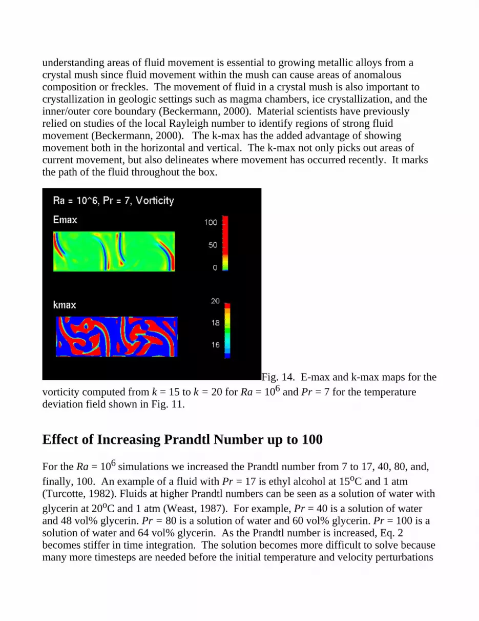
understanding areas of fluid movement is essential to growing metallic alloys from acrystal mush since fluid movement within the mush can cause areas of anomalouscomposition or freckles. The movement of fluid in a crystal mush is also important tocrystallization in geologic settings such as magma chambers, ice crystallization, and theinner/outer core boundary (Beckermann, 2000). Material scientists have previouslyrelied on studies of the local Rayleigh number to identify regions of strong fluidmovement (Beckermann, 2000). The k-max has the added advantage of showingmovement both in the horizontal and vertical. The k-max not only picks out areas ofcurrent movement, but also delineates where movement has occurred recently. It marksthe path of the fluid throughout the box.

Fig. 14. E-max and k-max maps for thevorticity computed from k = 15 to k = 20 for Ra = 106 and Pr = 7 for the temperaturedeviation field shown in Fig. 11.

Effect of Increasing Prandtl Number up to 100

For the Ra = 106 simulations we increased the Prandtl number from 7 to 17, 40, 80, and,finally, 100. An example of a fluid with Pr = 17 is ethyl alcohol at 15oC and 1 atm(Turcotte, 1982). Fluids at higher Prandtl numbers can be seen as a solution of water withglycerin at 20oC and 1 atm (Weast, 1987). For example, Pr = 40 is a solution of waterand 48 vol% glycerin. Pr = 80 is a solution of water and 60 vol% glycerin. Pr = 100 is asolution of water and 64 vol% glycerin. As the Prandtl number is increased, Eq. 2becomes stiffer in time integration. The solution becomes more difficult to solve becausemany more timesteps are needed before the initial temperature and velocity perturbations

cause convective movement. The overall time development of the solution evolvesslower. We also found that, as the Prandtl number was increased from Pr = 7, sharpertemperature gradients and stronger shear flows, i. e., velocity boundary layers developed. This required using more grid points and smaller timesteps. This further increased thecomputation time required for the simulations.

The most noticeable effect of even a small in increase in Prandtl number from 7 to 17 atRayleigh number 106 is the increase in horizontal shear flow (Fig. 15). This results in a"wind" driving the plumes. This shearing effect due to inertia could be substantial in asystem such as Europa where there is an icy "lithosphere" being deformed by aconvecting, brine-rich, global ocean. If the dissolved species in the ocean and theformation of ice increase the Prandtl number of the system, estimates on the behavior ofthe system based on studies at Prandtl number 7 may not be appropriate, and we must usehigher Prandtl numbers going upwards to 50 or 100.

Fig. 15. Long-term solution of thetemperature deviation and vorticity fields for Ra = 106 and Pr = 17.

The smaller scale structures resulting from the strong horizontal shear flow makes itdifficult to pick out the number of convection cells from the vorticity field in Fig. 15. This a situation where the wavelet transform proves especially valuable. In the largescale vorticity scalogram slice (Fig. 16), we can easily see that the same pattern of twowide convection cells separated by two narrow ones that we saw in simulations for Ra=106 and Pr =7 (Fig. 13). The features related to the shear are discerned clearly in the

medium and small-scales.


The E-max map for the smaller scales of the of the vorticity (Fig. 17) gives a similarpicture to the small-scale scalogram slice. The E-max, however, shows that the strongestsignatures are coming from two layers of circulation cells, one in the top of the fluid andone in the bottom. The horizontal shear in this fluid appears to be creating a layeredconvection style in the smaller scale. Vortex cells with positive sense of circulation havemuch stronger signatures than those with negative sense of circulation. The originalvorticity field (Fig. 15) also shows stronger positive vortices than negative ones. Thek-max map (Fig. 16) emphasizes both the vertical shearing movement of the fluid alongwith its significant horizontal component. The ability to pick out both the horizontal andvertical movement within the time-dependent fluid motions provides an advantage overthe more traditional local Rayleigh number approach, which only emphasizes the verticalmovement (Zaleski, 2000).

Fig. 17. E-max and k-max maps for thevorticity computed from k = 15 to k = 20 for Ra = 106 and Pr = 17 for the temperatureperturbation field shown in Fig. 15.

As the Prandtl number is increased to 100, the lateral temperature distribution showsmore layered structures. This indicates that there is better homogenization of the totaltemperature field within each layer (Fig. 18). Both the hot and cold thermal boundarylayers decrease in thickness. The plume heads still spread laterally across the hot andcold boundary layers, but they have less vertical thickness. This indicates the possibilitythat the Prandtl number may have an important control over the vertical heat flux infinite, but large Prandtl number convection.


The vorticity field undergoes noticeable changes with increasing Prandtl number (Fig.18). Individual circulation cells are delineated weakly by strong vertical shear layersalong their edges. The large-scale slice of the vorticity scalogram shows that there areonly two convection cells (Fig. 19) rather than the four seen for smaller Prandtl numbers. One of the convection cells is 1.5 times wider than the other. Although at first glance itmay appear that the scalogram shows three convection cells, this is due to the fact that thecontinuous convection field has been cut along the box edges. We see clearly that thereare actually two convection cells in the medium scalogram slice, where one can see theshear layers along the vertical edges of the cells. The medium and small scale scalogramslices show sharp vertical shear layers along the larger convection cell boundaries alongwith smaller convection cells embedded within the larger ones.

Fig. 19. Scalogram of the Ra = 106 andPr = 100, associated with the long-term solution of the vorticity field in Fig. 18.

The E-max map (Fig. 20) for the smaller scales portrays areas of sharp vertical shearlayers, which coincide with long narrow circulation cells seen in the medium-scalescalogram slice. These long narrow cells are found in between the larger scalecirculation cells. The k-max (Fig. 20) emphasizes the primarily vertical nature of fluidmotions; although it shows that there is also some degree of horizontal movement.


Effect of Increasing Rayleigh Number

Simulations were run at a Rayleigh number of 108 for Prandtl numbers of 7, 17, 40, 60,80, and 100. The increase in Rayleigh number leads to development of smaller scalestructures (Animation 2). The convection evolves through the branching of plumes andthe division and recoalescence of vorticity cells. The plumes become thinner than for Ra= 106. The temperature deviation is more layered, thus indicating a greater separation ofthe convective field. The shear layers along the edges of the convection zones are muchsharper.

Animation 2. Temporal Evolution of Ra = 108 and Pr = 7 simulation for an aspect-ratio of 3.

Click on picture below to start animation.

For Ra = 108 and Pr = 7, the convection pattern in the long time regime (Fig. 21) issimilar to the pattern for Ra = 106 and Pr = 100 (Fig. 18). There is one upwelling andone downwelling, both of which travel across the complete vertical distance between thehorizontal boundary layers. The vorticity is characterized by two circulation cells withone cell 1.5 times larger than the other. The vorticity field is also characterized by manysmall-scale features deriving from the larger convection cells.


By comparing the temperature deviation scalogram for convection in a Prandtl number 7fluid at Ra = 108 (Fig. 22) to that in a fluid with Ra = 106 (Fig. 12), we can see the

variations of the scales associated with the plumes. For Ra = 106, the general shape ofthe plumes is visible in the medium-scale. In the medium-scale for Ra = 108, we can seehot regions in the boundary layer where the plumes impinge, but there are only fainttraces of the plume stems in the medium-scale. The full details of the plumes are visibleonly at the smaller scale for Ra = 108 .

Fig. 22. Scalogram of the temperaturedeviation for the Ra = 108 and Pr = 7, associated with the long-term solution of thetemperature deviation field in Fig. 21.

Wavelet analysis becomes invaluable in analyzing the complicated vorticity fieldsproduced in higher Rayleigh number convection (Ra = 108) (Fig. 23). In the large-scalescalogram slice we can see the structure of the two large convection cells. Themedium-scale slice gives us the smaller convection cells within the larger cells; while thesmall-scale slice shows the small-scale shear layers lying along the edge of thelarge-scale circulation cells.


Since a large portion of the activity in this vorticity pattern occurs at the smallest scales,it is useful to examine the E-max over the small-scales, from mode k = 15 to k = 20 (Fig.24). The plume signatures that were also visible in the small-scale scalogram slice arehighlighted along with he vortices within the larger convection cells. These vorticesoccur over a range of smaller scales. The k-max map (Fig. 24) shows a finer pattern thanfound in the k-max maps for the simulations at Ra = 106. The vertical and horizontalmovements associated with the plume and the downwelling coexist with the movementassociated with the smaller vortices within the two larger circulation cells.


The temperature and vorticity fields at Ra = 108, Pr = 17 and 40 are somewhat similar tothose for Ra = 108, Pr = 7. When the Prandtl number is increased to 60 at Ra = 108,however, the convection style changes dramatically (Fig. 25). The temperaturedeviation field becomes more layered, indicating better homogenization of thetemperature within each layer. The vorticity field has become quite complicated, and it isdifficult to interpret these fields without the use of wavelets.


The change in the convection style when the Prandtl number is increased from 7 to 60becomes clearly evident in the temperature deviation scalogram (Fig. 26). We do not seeany signatures from plumes or downwellings in the large-scale. In the medium-scale, weonly see the boundary layers. The boundary layer signatures are broken by numeroussmall upwellings and downwellings. The shape of these upwellings and downwellings isonly apparent in the small-scale. We can see that these features do not traverse verticallythrough the center of the box. A layered convection style has developed with anadditional internal boundary layer across the center of the box.

Fig. 26. Scalogram of the Ra = 108 andPr = 60, associated with the long-term solution of the temperature deviation field in Fig.25.

The large-scale slice of the vorticity scalogram shows that large-scale circulation cellsstill exist at this mediumly large Prandtl number (Fig. 27). There are four circulationcells, which are much narrower than the large-scale circulation cells at lower Prandtlnumbers. The medium-scale scalogram slice shows a complex structure of circulationcells within the large-scale circulation cells. The small-scale slice of the vorticityscalogram is almost identical to the small-scale slice of the temperature deviationscalogram (Fig. 26) . There are areas of downwellings and upwellings associated withsharp shear layers that travel vertically to the center of the box. Large plumes that travelthrough the vertical distance of the box no longer exist. We note that this change inconvection style is brought about by increasing the Prandtl number, while keeping theRayleigh number constant. This indicates that the Prandtl number plays a significant rolein determining the convection style. The relative increase in viscosity to thermaldiffusivity as the Prandtl number increases makes the movement of large-scale plumesand downwelling more difficult. More of the heat appears to be transported by smallerscale plumes at higher Prandtl numbers.


The E-max of the vorticity field shows the location of the shear layers of the strongerplumes and downwellings (Fig. 28). The heads of the plumes and downwellings haveespecially strong signatures. We also see the layered structure of the convection with noplumes crossing the entire box. The k-max map for Ra = 108 and Pr = 60 is quitedifferent from that of Ra = 108 and Pr = 7. We can see evidence of a large amount ofhorizontal movement, but only limited vertical movement. Although many of thestructures do not cross the center of the box, it appears that there is still some movementacross the center. This indicates that the convection style is not completely layered.

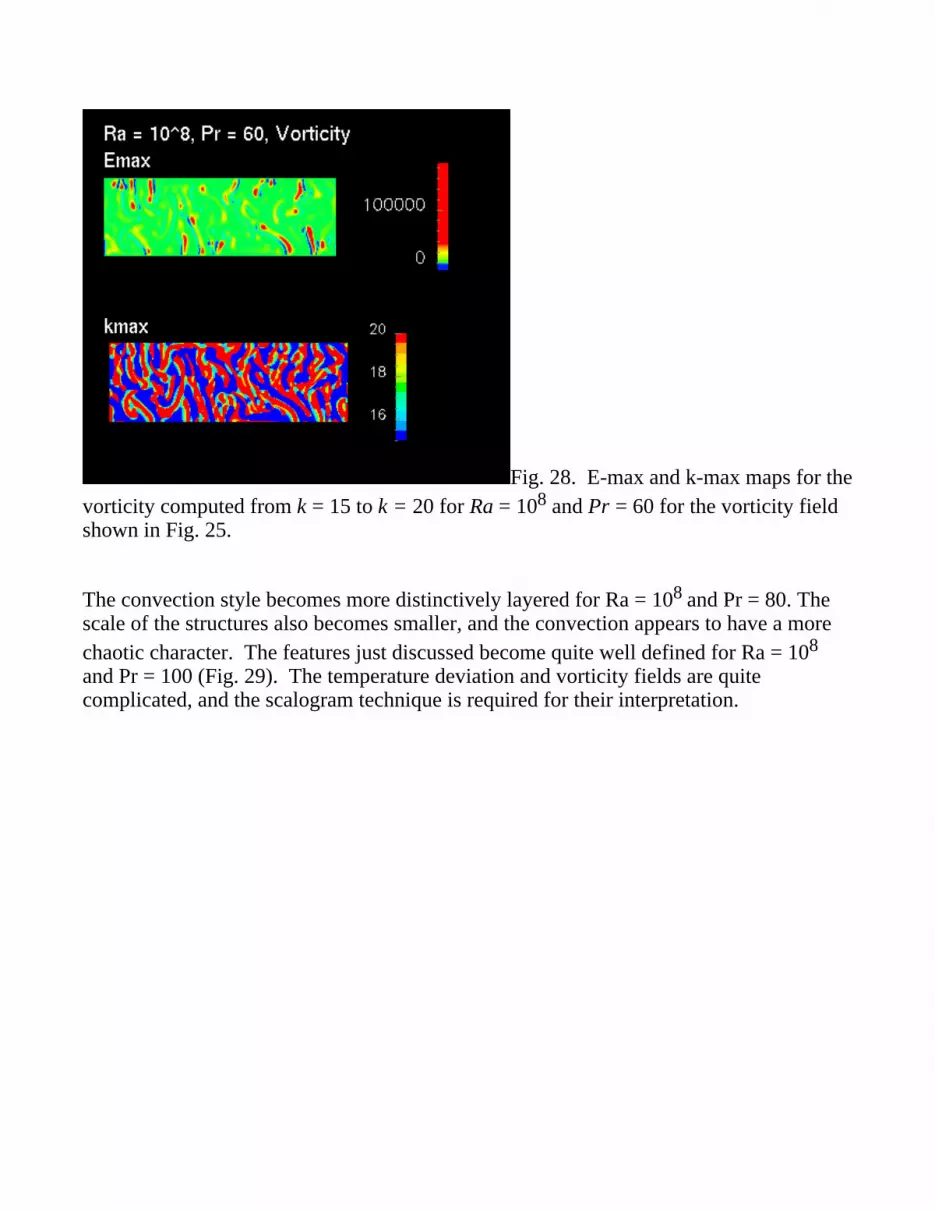
Fig. 28. E-max and k-max maps for thevorticity computed from k = 15 to k = 20 for Ra = 108 and Pr = 60 for the vorticity fieldshown in Fig. 25.

The convection style becomes more distinctively layered for Ra = 108 and Pr = 80. Thescale of the structures also becomes smaller, and the convection appears to have a morechaotic character. The features just discussed become quite well defined for Ra = 108

and Pr = 100 (Fig. 29). The temperature deviation and vorticity fields are quitecomplicated, and the scalogram technique is required for their interpretation.

Fig. 29. Long-term solutiontemperature deviation and vorticity fields for Ra = 108 and Pr = 100.

The slice showing the vorticity scalogram for the large-scale slice (Fig. 30) displays thatthere are still some large circulation cells. There are basically two layers of large-scalecells; the convection style has become indisputably layered. The convection cells aretilted, indicating the presence of horizontal shear. The medium-scale scalogram sliceshows a complicated pattern of narrow, tilted convection cells. This confirms thepresence of a horizontal shear. The small-scale slice shows the small shear layers createdby individual plumes. We can see that the plumes fade away when they reach abouthalfway through the box height. A new boundary layer has been formed across themiddle of the box by the presence of layered convection.


The small scalogram slice is complicated for this simulation. Although it only looks at k= 20, the amount of small-scale features in this vorticity field indicates that other smallscales should play an important role. We have examined the E-max over scales rangingfrom k= 15 to 20 (Fig. 31). In this image we can see both the long narrow shear layersalong the edges of larger convection cells and the smaller scale vortices that are furthersubdividing the vortices observed in the medium-scale. The vortices with scales rangingfrom medium to small indicate that although the convection still has some large-scale oforganization, the smaller scales are becoming increasingly important. The k-max (Fig.31) emphasizes the chaotic movement throughout the box. There is less movementacross the center of the box than for Ra = 108 and Pr = 60. This indicates that theconvection style is reaching a truly layered state for this intermediately high Prandtlnumber situation.

Fig. 31. E-max and k-max of Ra = 108

and Pr = 100 for k = 15 to 20 of the long-term solution of the vorticity field in Fig. 29.

Reynolds Number

The turbulent Reynolds number was calculated a posteriori for several of the simulations(Table 3). The Reynolds number was calculated by post-processing the data from therun. The Reynolds number was not calculated from an assumed Rayleigh and Prandtlnumber relationship.

The Reynolds number is defined as:

(8)

where V is the dimensional root-mean-square velocity, l is the dimensional velocity, and is the dimensional kinematic viscosity.

We calculated the Reynolds number a posteriori as:

(9)

V0 is the nondimensional root-mean-square or quadratic mean velocity. It represents the

velocity of the largest eddies. l0 is the nondimensional integral length scale or

autocorrelation length. It represents the size of the largest eddies. V0 and l0 are local

quantities that are calculated in the course of the run. Since V0 and l0 are

nondimensionalized by the thermal diffusivity and the box height, the resulting Reynoldsnumber is that defined in Eq. (8).

RayleighNumber

Prandtlnumber Aspect-Ratio

ReynoldsNumber*

106 40 3 2.2

106 80 3 0.63

106 100 3 0.45

Table 3. Reynolds numbers for several simulations. * indicates that the Reynoldsnumbers were calculated a posteriori after each run.

The Reynolds numbers tended to decrease with Prandtl number for Ra = 106, which is inthe low Reynolds number regime for these Prandtl numbers. There are two effectscontributing to the decrease in Reynolds number with Prandtl number. The first is thedirect effect of dividing the quantities V0 and l0 by the Pr. The second effect is the that

V0 * l0 tended to decrease with Prandtl number. The smaller size of the eddies with

increasing Prandtl number was also picked up visually on the scalogram (e.g. Fig. 19 &30).

Three-Dimensional Convective Effects

The systems discussed in this study are all two-dimensional. In 2-D systems the vorticityvector is always perpendicular to the flow plane. This means that no vortex stretchingcan occur in 2-D flows since the vorticity cannot be amplified by the velocity gradient. Vorticity can only be weakened by viscous dissipation. A fundamental difference in thenature of turbulence in 2-D and 3-D flows is that energy in large vortices cannot betransported to smaller scale vortices through vortex stretching; instead in 2-D energy at agiven scale is transferred to larger scales and dissipated at the system boundaries(Belmonte, et al., 2000). Due to the absence of vortex stretching, it is more likely thatfluctuations will be transported downstream intact in 2-D than in 3-D flow (Belmonte, etal., 2000). Lateral mixing effects that can remove and introduce fluctuations would alsobe weaker in 2-D than in 3-D flow (Belmonte, et al., 2000).

Three-dimensional effects have important influences on geophysical systems. Thevertical velocity introduced by buoyancy in atmospheric flows induces vortex stretchingthat is responsible for the spiraling updrafts and downdrafts seen in thunderstorms anddust whirls (Cortese and Balachander, 1993). For systems such as Europa’s global ocean,rotation caused by Coriolis effects may have limit how far plumes can spread laterally(Thomson and Delaney, 2001). One type of flow that is characterized by the formationof cigar-shaped vortices through vortex stretching is known as ABC flow (Aref andBrøns, 1998, Dombre et al., 1986). The stretching ability of these flows leads to theirability to amplify magnetic fields and form dynamos (Galloway and Frisch, 1986). Thistype of flow has been suggested as a mechanism for dynamo production in the Sun(Dorch, 2000). Vortex stretching flows also are responsible for dynamos produced in theouter core of the Earth and the oceans of the Jovian moon Callisto and Europa (Khurana,et al., 1998). We will conduct future studies on 3-D finite Prandtl flows to furtherenhance our understanding of these important flows in geophysical systems.

Schmalzl et al. (2001) found that 3-D effects are most important in flows with Prandtlnumbers below 3 when Ra = 106 due to the fact that the toroidal flow, which is neglectedin 2-D flow. They found two flow regimes. In the regime at Prandtl numbers below 3,rising currents are distorted by toroidal currents leading to distortion of currents andexchange of heat between plumes and the interior. This results in diffusion being themain mechanism of heat flux. As the Prandtl number increased, the toroidal flowdecreased, and most of the heat was transported by plumes through the isothermal interiorto thermal boundary layers.

The simulations of Schmalzl et al. (2001) were done at Ra = 106. Rescaling theconvection equations by the free fall velocity rather than the thermal diffusivity gives abetter understanding of the effect of increasing the Rayleigh number on the toroidalflow. The free fall velocity is given by:

(10)

where is the coefficient of thermal expansion. The conservation of momentumequation nondimensionalized by the free fall velocity is:

(11)

As the Rayleigh number increases, the diffusional term will drop out of the conservationof momentum equation for Pr/Ra < 10-8. The change in poloidal velocity with time canthen be expressed as:

(13)

and the change in toroidal velocity in time can be expressed as:

(14)

The toroidal velocity, therefore, should not have a significant effect at Rayleigh numbersof about 108 for Prandtl number of around 3. In short, the toroidal motions should besaturated at high Rayleigh numbers under the conditions prescribed in Eqs. 13 and 14.

Conclusions

We have found that at a given Rayleigh number, increasing the Prandtl number can causethe convection style to change from non-layered to layered. Other effects of increasingthe Prandtl number at a given Rayleigh number include an increase in the number ofplumes, a thinning of the plumes and boundary layers, and an increase in the horizontalshear. The overall size of the large eddies tend to decrease with Prandtl number. This ispartially responsible for the decrease in Reynolds number with Prandtl number.

As the Rayleigh number and Prandtl number were increased, the vorticity fields becamemore complicated. The wavelet transform helped us interpret these fields by allowing usto separate out the processes occurring at different scales without losing the specificspatial location of the signals (van den Berg, 1999). This allows us to see the overalllarge-scale convection style even when it is masked by small-scale structures. The largescale scalogram slices were used to pick out large-scale circulation cells and layeredstructures. The small-scale scalogram slices allowed us to separate out smaller scaleprocesses, such as shear zones along circulation cell edges and smaller vortices withinlarger circulation cells.

The E-max and k-max distributions were used to synthesize the data in the scalogram(Bergeron, 2000). The E-max gives the energy for the scale that has the maximumenergy over a given range of scales. It allows one to quickly find the most prominentfeature in that scale range. We found it useful for quickly picking out features, such asshear zones at the smaller scales where there was often signals from many sources. Itwas especially helpful for simplifying vorticity datasets in simulations at higher Rayleighand Prandtl numbers where a large number of vortices occurred over a wide range ofscales.

The k-max maps out areas of sharp gradients. It was used to draw a path of fluidmovement through the box. The k-max could be used in simulations of crystal mushes topick out areas of movement where anomalous compositions might occur in the solidifiedfluid. Identifying areas of possible anomalous compositions is important in the casting ofmetallic alloys and may also prove useful in modeling flow in crystal mushes in magmachambers, the inner and outer core boundary, and sea ice (Beckermann, 2000).

We have found four major styles of convection in the long-term solutions for simulationswith an aspect-ratio of 3. For Ra =106 and Pr = 7 to 80, there are four convection cells:two wide cells separated by two narrow cells. For Ra =106 and Pr = 100 and Ra =108

and Pr = 7 to 17, there are two convection cells with one cell that is about 1.5 timeswider than the other cell. At Prandtl number 60 there are 4 narrow convection cells. Amajor change in convection style is evident at Pr = 60. The increasing relative viscosityresults in more heat being transported by small-scale thermal plumes than by large-scaleplumes. At Ra =108 and Pr = 100 the four narrow cells divide into two layers of cells,and the convection style becomes layered. This study indicates that the convection styleis dependent on both the Rayleigh number, Prandtl number. We will conduct futurestudies in 3-D to help determine the effect of the third dimension on these flows.

Since increasing the Prandtl number can greatly increase the shear in the fluid, thePrandtl number of the fluid may have significant effects on the type of deformation seenin a "lithospheric" layer above a convecting finite Prandtl fluid. For example a largeshear force created in the convecting brine-rich ocean of Europa (Carr et al., 1998,Khurana et al., 1998) could explain some of the surface deformation seen on this Jovianmoon.

We have also found that an increase in Prandtl number can have a large influence on boththe thickness of the boundary layers and the overall convection style, the scale at whichplumes develop, the number of convection cells, and whether or not convection islayered. Wavelets have allowed us to analyze the convection simulations at differentscales to better understand these changes in convection style. The change in convectionstyle with Prandtl number indicates that the Prandtl number has a significant effect on theheat flux in the fluid. We have seen that the Prandtl number should be important in theNusselt number scaling (Grossmann and Lohse, 2000, Zaleski, 2000, Verzzico andCasmussi, 1999, Shairman and Siggia, 1990, Castaing et al., 1989). Future studies willexamine quantitatively the dependence of the Nusselt number on the Prandtl number. Abetter understanding of heat flux in finite Prandtl number convection will lead to a betterunderstanding of the heat budget of planetary bodies with convecting global oceans suchas the Jovian moon Europa. It will also allow a better understanding of heat flux on theearly Earth during the magma ocean period. The style of convection in this magma oceanmay also be important to the chemical differentiation of the early Earth.

Acknowledgments

We would like to acknowledge Alain P. Vincent, David Munger, Ludek Vecsey, andFabien Dubuffet for their help with this study. Catherine Hier Majumder thanks the NSFFellowship program for providing support during this study. This research was alsosupported by the Complex Fluids Program of D. O. E.

References

Aref, H. and M. Brøns (1998). On stagnation points and streamline topology in vortexflows. Journal of Fluid Mechanics. Vol. 370. pp. 1-27.

Beckermann, C. (2000). Modeling of macrosegregation: past, present, and future. Flemings Symposium. Boston, MA.

Belmonte, A., B. Martin, and W. I. Goldburg (2000). Experimental study of Taylor’shypothesis in a turbulent soap film. Physics of Fluids. Vol. 12, pp. 835-845.

Bergantz, G. W. (1992). Conjugate solidification and melting in multicomponent openand closed systems. International Journal of Heat and Mass Transfer. Vol. 35:533-543.

Bergeron, S. Y., A. P. Vincent, D. A. Yuen, B. J. S. Tranchant, and C. Tchong. (1999). Viewing seismic velocity anomalies with 3-D continuous Gaussian wavelets. Geophysical Research Letters. Vol. 26: 2311-2314.

Bergeron, S. Y., D. A. Yuen, and A. P. Vincent (2000). Looking at the inside of theEarth with 3-D wavelets: a pair of new glasses for geoscientists. Electronic Geosciences. Vol. 5.

Carr, M. H., M. J. S. Belton, C. R. Chapman, M. E. Davies, P. E. Geissler, R. J.Greenberg, A. S. McEwen, B. R. Tufts, R. Greeley, R. J. Sullivan, J. W. Head III, R. T.Pappalardo, K. P. Klaasen, T. V. Johnson, J. Kaufman, D. A. Senske, J. M. Moore, G.Neukum, G. Schubert, J. A. Burns, P. Thomas, J. Veverka (1998). Evidence for asubsurface ocean on Europa. Nature. Vol. 391: 363-365.

Castaing, B., G. Gunaratne, F. Heslot, L. Kadanoff, A. Libichaber, S. Thomae, X. Z. Wu,S. Zaleski and G. Zanetti (1989). Scaling of hard thermal turbulence in Rayleigh-Bénard convection. Journal of Fluid Mechanics. Vol. 204: 1-30.

Castillo, J., A. Mocquet, and G. Saracco (2001). Wavelet transform: a tool for theinterpretation of upper mantle converted phases at high frequency. GeophysicalResearch Letters, Vol. 28, pp. 4327-4330.

Chao, B. F. and I. Naito (1995). Wavelet analysis provides a new tool for studying Earth’s rotation. E. O. S. Vol. 76. pp. 161 & 164.

Cortese, T. and S. Balachandar (1993). Vortical nature of thermal plumes in turbulent convection. Physics of Fluids A. Vol. 12. pp. 3226-3232.

Daubechies, I. (1992). Ten Lectures on Wavelets. Society for Industrial and AppliedMathematics, Philadelphia, 357 pp.

Dombre, T. U. Frisch, J. M. Greene, M. Hénon, A. Mehr, and A. M. Soward (1986). Chaotic streamlines in the ABC flows. Journal of Fluid Mechanics. Vol. 167. pp.353-391.

Dorch, S. B. F. (2000). On the structure of the magnetic field in a kinematic ABC flow dynamo. Physica Scripta. Vol. 61. pp. 717-722.

Galloway, D. and U. Fricsh. (1986). Dynamo action in a family of flows with chaotic streamlines. Geophysical and Astrophysical Convection. Vol. 36. pp. 53-83.

Glatzmaier, G. A. and Roberts, P. H. (1995). A three-dimensional self-consistentcomputer simulation of a geomagnetic field reversal. Nature. Vol. 377. pp. 203-209.

Grossmann, S. and D. Lohse (2000). Scaling in thermal convection: a unifying theory. Journal of Fluid Mechanics. Vol. 407: 27-56.

Hier, C. A., S. Y. Bergeron, D. A. Yuen, E. O. Sevre and J. M. Boggs. Thermal convection in finite Prandtl number fluids at high Rayleigh number. Electronic Geosciences. Vol. 6.

Khurana, K. K., M. G. Kivelson, D. J. Stevenson, G. Schubert, C. T. Russell, R. J. Walker, and C. Polanskey (1998). Induced magnetic fields as evidence for subsurface oceans on Europa and Callisto. Nature. Vol. 195: 777-780.

Kirk, R. L. and D. J. Stevenson (1987). Thermal evolution of a differentiated Ganymede and implications for surface features. Icarus. Vol. 69: 91-134. Shraiman, B. I. and E. D. Siggia (1990). Heat transport in high-Rayleigh number convection. Physical Review A. Vol. 42: 3650-3653.

Malamud, B. D. and D. L. Turcotte (2001). Wavelet analyses of Mars polar topography. Journal of Geophysical Research. Vol. 106. pp. 17497-17504.

Resnikoff, H. L. and R. O. Weiss, Jr. (1998). Wavelet Analysis: The Scalable Structure

of Information. Springer-Verlag, New York, 435 pp.

Schmalzl, J., M. Breuer, and U. Hansen (2001). The influence of the Prandtl number onthe style of vigorous thermal convection. Submitted to: Geophysical and AstrophysicalFluid Dynamics.

Shevtsova, V. M.. D. E. Melnikov, and J. C. Legros. Three-dimensional simulations ofhydrodynamic instability in liquid bridges: influence of temperature-dependent viscosity. Physics of Fluids. Vol. 13. pp, 2851-2865.

Shraiman, B. I. and E. D. Siggia (1990). Heat transport in high-Rayleigh numberconvection. Physical Review A. Vol. 42. pp. 3650-3653/

Thomson, R. E. and J. R. Delaney (2001). Evidence for weakly stratified Europan ocean

sustained by seafloor heat flux. Journal of Geophysical Research. Vol. 106. pp. 12355-12365.

Turcotte, D. L. and G. Schubert. Geodynamics. p. 233. John Wiley & Sons, New York.

van den Berg, J. C., ed. (1999). Wavelets in Physics. Cambridge, New York, 453 pp.

Vecsey, L. and C. Matyska (2001). Wavelet spectra and chaos in thermal convection modelling. Geophysical Research Letters. Vol. 28. pp. 395-398.

Verzicco, R. and R. Camussi (1999). Prandtl number effects in convective turbulence. Journal of Fluid Mechanics. Vol. 383: 55-73.

Vincent, A. P. and D. A. Yuen (1999). Plumes and waves in two-dimensional turbulent thermal convection. Physical Review E. Vol. 60:2957-2963.

Yuen, D. A., A. P. Vincent, S. Y. Bergeron, F. Dubuffet, A. A. Ten, V. C. Steinbach, and L. Starin (2000). Crossing of scales and non-linearities in geophysical processes. In: Problems in Geophysics for the New Millennium, Eds. E. Boschi, G. Ekström, and A. Morelli. pp. 403-462.

Weast, R. C. Ed. (1987). Handbook of Chemistry and Physics. Ed. 68. p. D-232. CRCPress, Boca Raton, FL.

Zaleski, S. (2000). The 2/7 law in turbulent thermal convection. In: Geophysical and Astrophysical Convection, Ed. P. A. Fox and R. M. Kerr. pp. 129-143, Gordon andBreach Science Publishers, Newark, NJ.

Zhang, K. and G. Schubert. (2000). Teleconvection: remotely driven thermal convection in rotating stratified spherical layers. Science. Vol. 290: 1944-1947.

Finite Prandtl Number 2-D Convection at High Rayleigh Number

Documents

Transcript of Finite Prandtl Number 2-D Convection at High Rayleigh Number