Is the Rayleigh-Sommerfeld diffraction always an exact

reference for high speed diffraction algorithms?

SOHEIL MEHRABKHANI,1,2 AND THOMAS SCHNEIDER1,2

1Terahertz-Photonics group, Institut für Hochfrequenztechnik, TU Braunschweig, Schleinitzstraße 22, 38106 Braunschweig 2Lena, Laboratory for Emerging Nanometrology

*Corresponding author: soheil.mehrabkhani@ihf.tu-bs.de

Abstract: In several areas of optics and photonics like wave propagation, digital holography, holographic microscopy, diffraction imaging, biomedical

imaging and diffractive optics, the behavior of the electromagnetic waves has to be calculated with the scalar theory of diffraction by computational

methods. Many of these high speed diffraction algorithms based on a fast Fourier transformation are in principle approximations of the

Rayleigh-Sommerfeld Diffraction (RSD) theory. However, to investigate their numerical accuracy, they should be compared with and

verified by RSD. All numerical simulations are in principle based on a sampling of the analogue continuous field. In this article we

demonstrate a novel validity condition for the well-sampling in RSD, which makes a systematic treatment of sampling in RSD possible.

We show the fundamental restrictions due to this condition and the anomalies caused by its violation. We also demonstrate that the

restrictions are completely removed by a sampling below the Abbe resolution limit. Furthermore, we present a very general unified approach

for applying the RSD outside its validity domain by the combination of a forward and reverse calculation.

1. Introduction

The Rayleigh-Sommerfeld diffraction (RSD) integral is used for the

calculation of scalar wave propagation. In contrast to approximations

such as Fresnel or Fraunhofer diffraction, the RSD gives an exact

solution for the output field of a given input field [1-3]. However, to

the best of our knowledge there is no general analytical solution for

the calculation of an exact RSD. Therefore, numerical methods have

to be used. In these methods, the RSD is treated as a Riemann

integral, which has to be discretized. Thus, with usual computational

power, only high speed algorithms make the utilization of the

diffraction theory possible. These high speed algorithms use

approximations of the RSD integral such as a quadratic phase [2, 4]

or a frequency-cut in convolution RSD [5-7] and in the angular

spectrum method (ASM) [6, 8-11]. Whereupon the latter is only

valid for small propagation distances [2, 12]. Contrary to the

Kirchhoff solution of the diffraction problem [2, 3, 13], the

mathematical solution of the RSD is not inconsistent when the

observation point is close to the diffracting screen. Thus, the

accuracy of the high-speed alternatives, even for very short

propagation distances, could be verified by referencing them with

exact solutions given by the RSD. Since there exist only a few

analytical solutions, an alternative is to compare them with a

discretized RSD. However, here we will demonstrate that the use of

the discretized RSD can cause enormous calculation errors. We will

give the boundary conditions for the usage of the discretized RSD

and show possibilities to completely remove the calculation errors.

2. Sampling condition for the Rayleigh-

Sommerfeld-diffraction

Figure 1 shows a typical setup for the calculation of the diffraction

problem. A coherent source, a laser, illuminates a small object in

plane 1. A discretized sensor like a CCD camera would see a

diffracted image of the object in plane 2 or 3.

According to the Rayleigh-Sommerfeld diffraction integral

the field distribution in an output plane 2 in the distance 𝑧12,

parallel to the input plane is [1-3]:

�⃗⃗⃗� 2 = �⃗⃗� 2 +𝑧12�̂�𝑧; 𝛼 = (𝑖𝑘−1

|�⃗⃗⃗� 2 − �⃗⃗� 1|)

𝑧12

|�⃗⃗⃗� 2 − �⃗⃗� 1|2

𝑢2 (�⃗⃗⃗� 2) = −12𝜋

∬𝑑2𝑟1𝛼𝑢1(�⃗⃗� 1)

Ω

𝑒𝑖𝑘|�⃗⃗⃗� 2−�⃗⃗� 1|

(1)

Figure 1: Coherent imaging of an object in the first (object) plane. The second and third

planes refer to the diffracted images of the object at the distance 𝑧12 and 𝑧13 from the

object plane, respectively.

Where 𝑢1(�⃗⃗� 1) is the field distribution in the input (object)

plane 1 and 𝑘 is the wave number. The two vectors �⃗⃗� 1, �⃗⃗� 2are

position vectors in plane 1 or 2, respectively.

For a numerical treatment of Eq.1, not only the input and

output plane but as well the propagation dependent harmonic

term 𝑒𝑖𝑘|�⃗⃗⃗� 2−�⃗⃗� 1| has to be sampled, according to the well-known

Nyquist sampling criterion [14]. Thus, the sampling

frequency must at least correspond to twice the highest

frequency contained in the harmonic term. If we consider the

phase of the propagation term as:

with the transversal Cartesian coordinates in the input (𝑥1, 𝑦1)

and output (𝑥2, 𝑦2) plane, the derivative of the phase 𝜑 results

in the spatial frequency of the propagation phase 𝑓:

𝑓𝑥 =1

2𝜋|𝜕𝜑

𝜕𝑥1

| =𝑘|𝑥1 − 𝑥2|

2𝜋√(𝑥1 − 𝑥2)2 + (𝑦1 − 𝑦2)

2 + 𝑧122

(3)

This spatial frequency is a monotonically increasing function

of |𝑥1 −𝑥2|. To get its maximum value the conditions

|𝑦1 −𝑦2| = 0 and |𝑥1 −𝑥2| = 𝑥1𝑓𝑝 + 𝑥2𝑓𝑝 must be fulfilled.

Here 𝑥1𝑓𝑝 and 𝑥2𝑓𝑝 are the distances of the farthest point from

the center in 𝑥-direction in the relevant computational plane 1

or 2 with nonzero amplitude value (see Fig. 1). Due to zero

values of the amplitude around the boundary, the maximum

width can be smaller than the real width of the computational

domain. Thus, it follows for the maximum spatial frequency

𝑓𝑥,𝑚𝑎𝑥 in 𝑥-direction:

𝑓𝑥,𝑚𝑎𝑥 =1

2𝜋|𝜕𝜑

𝜕𝑥1

|𝑚𝑎𝑥

=𝑥1𝑓𝑝 + 𝑥2𝑓𝑝

𝜆√(𝑥1𝑓𝑝 + 𝑥2𝑓𝑝)2+ 𝑧12

2

(4)

The sampling frequency 𝑓s is related to the sampling spacing

via 𝛿𝑥1 = 1/𝑓s. Thus, it follows for the sampling according to

the Nyquist criterion (𝑓s ≥ 2𝑓𝑚𝑎𝑥):

Therefore, the validity condition for the numerical treatment

of the RSD can be written as:

Consequently, for a given sampling spacing 𝛿𝑥1 , 𝛿𝑦1 in the

object plane and a maximum size 𝑥1𝑓𝑝 , 𝑦1𝑓𝑝 of the object and

its image 𝑥2𝑓𝑝, 𝑦2𝑓𝑝 in the output computational plane, there is

a critical minimum propagation distance 𝑧1 allowed, in which

the output plane can be calculated by:

An analog derivation results in a similar condition for the 𝑦-

direction:

Thus, the condition for the minimum propagation distance

(critical distance) is:

The critical distance is the minimum distance in which an

output field (image) can be numerically calculated by RSD

without violating the Nyquist criterion for the interplay of the

sampling conditions of input and output planes and the

distance. The reconstruction of the object from the diffracted

image is only possible, if the Nyquist theorem is fulfilled in

the reverse direction too. This results in equations analogous

to (7), (8) and (9) with reversed index 1 and 2.

Thus, the total critical distance 𝑧c for a forward and reverse

transformation of the field has to be at least 𝑧c = 𝑚𝑎𝑥 (𝑧1c,𝑧2c), which is the proposed validity condition for a numerical

treatment of the RSD.

According to the validity condition, the correct calculation of the

diffraction pattern and also the reconstruction of the original object

from the achieved pattern may be performed if the propagation

distance is longer than the critical distance:

𝑧12 > 𝑧c (10)

𝜑 = 𝑘|�⃗� 2 − 𝑟 1| = 𝑘√𝑅22 + 𝑟1

2 − 2�⃗� 2 ∙ 𝑟 1

= 𝑘√𝑥22 + 𝑦2

2 + 𝑧122 +𝑥1

2 + 𝑦12 − 2(𝑥1𝑥2 + 𝑦1𝑦2) (2)

(2)

1

𝛿𝑥1

≥ 2𝑥1𝑓𝑝 + 𝑥2𝑓𝑝

𝜆√(𝑥1𝑓𝑝 + 𝑥2𝑓𝑝)2+ 𝑧12

2

(5)

𝑧122 ≥ (

4𝛿𝑥12

𝜆2

−1)(𝑥1𝑓𝑝 +𝑥2𝑓𝑝)2

(6)

𝑧1c𝑥2 = (

4𝛿𝑥12

𝜆2

−1)(𝑥1𝑓𝑝 +𝑥2𝑓𝑝)2

(7)

𝑧1c𝑦2 = (

4𝛿𝑦12

𝜆2

−1)(𝑦1𝑓𝑝 +𝑦2𝑓𝑝)2

(8)

𝑧1c = 𝑚𝑎𝑥(𝑧1𝑐𝑥 , 𝑧1𝑐𝑦)

(9)

However, it does not mean that the full information of the object can

be obtained from the diffracted image in the output plane. This

depends on the numerical aperture of the output plane as well.

3. Investigation of the validity condition

A. Anomalies if 𝒛 < 𝒛𝒄

To show the influence of the violation of the aforementioned

validity condition we have used an amplitude object (constant

phase) as described in Fig. 2 (a) and (b) and calculated its

diffraction pattern at a distance 𝑧 < 𝑍𝑐. For the sake of simplicity

but without loss of generality, the phase distributions are compared

indirectly. Thus, the magnitude and real part of the complex

amplitude will be discussed throughout the paper. As can be seen

in Fig. 2, for this object both values are identical because it

has a zero phase. The color-bar shows the normalized

amplitude and real part values.

Figure 2: Input object plane, (a) magnitude and real part (b) of the complex amplitude.

If not otherwise stated, the following parameters were used for the presented

simulations: Wavelength 𝜆 = 0.633 𝜇𝑚, sampling spacing in the input plane 𝛿𝑥1 =𝛿𝑦1 = 0.76 𝜇𝑚 and in the output plane 𝛿𝑥2 = 𝛿𝑦2 = 0.94 𝜇𝑚. The pixel numbers

in the x and y axis as well as in the input and output plane are the same 𝑁1,2,𝑥,𝑦 = 265.

The width of the computational domain in the input plane is 𝑃𝑥1= 𝑃𝑦1

= 201 𝜇𝑚,

whereas for the output plane it is 𝑃𝑥2= 𝑃𝑦2

= 250 𝜇𝑚.

The simulated distance between the object and the image plane

is 𝑧12 = 20 𝜇𝑚 which, according to Eqs. (7 - 9), is much smaller

than the critical distance 𝑧𝑐 = 534 𝜇𝑚. The calculated

amplitude and real part of the diffracted field 𝑢12 at a

distance 𝑧12 can be seen in Fig. 3 (a) and (b) respectively. The

error due to the violation of the validity condition can be seen

by a reconstruction of the original object from the diffracted

image 𝑢12. Thus, the reverse RSD 𝑧21 has to be applied. Here

the term “reverse” instead of “inverse” transform will be used

in order to avoid confusion.

The result can be seen in Fig. 3 (c) and (d). A similar pattern

like in the original object occurs but, with very strong

anomalies. Especially the nonzero values of the field in areas,

which originally exhibit zero values, lead to completely

wrong results. The correlation coefficient 𝑟 between 𝑢1 and

𝑢121, i.e. the field after transforming from position 1 to 2 and

back to 1 is 𝑟 = 0.72 and 𝑟 = 0.75 for the magnitude of the

complex field and its real part, respectively. The obviously

strong deviation to the input is a consequence of the

insufficiency of the propagation distance 𝑧 < 𝑧𝑐 .

Figure 3: Reconstruction errors for 𝑧 < 𝑧𝑐 (a) magnitude and (b) real part of the complex amplitude of the diffracted image in plane 2. (c) and (d) magnitude and real

part of the reconstructed object in plane 1.

B. Propagation distance z >𝒛𝒄

As derived in section 1, if the condition 𝑧12 > 𝑧c is satisfied

for the numerical calculation of the RSD, there will be no loss

of information due to the transformation. For an object with a

fixed sampling spacing the critical propagation distance is

fixed. Accordingly, if the propagation distance is longer

than 𝑧c, a correct treatment of the computational RSD should

be achieved for the given sampling spacing.

In Fig. 4 (a) and (b) the diffracted image is numerically

calculated by the RSD under the assumption that the

propagation distance 𝑧13 = 730 𝜇𝑚 satisfies the validity

condition. To confirm the correctness of the field 𝑢13 in the

plane 3 as a necessary condition, the reverse transform is

considered to reconstruct the input object in the input plane,

as reported in Fig. 4 (c) and (d). The correlation coefficient

is 𝑟 = 0.97 for both, magnitude and real part of the complex

amplitude. Since a small part of the whole information will be

lost by the spatial limitation of the computational plane, it is

smaller than one. Comparing the correlation coefficients for

the reconstructed object in Fig. 3 and Fig. 4 shows a more than

20% improvement. Therefore, at the distance 𝑧13 almost the

whole information of the object plane is preserved. However,

in some cases the RSD might be applied as a reference for

different algorithms at a propagation distance outside of the

validity domain.

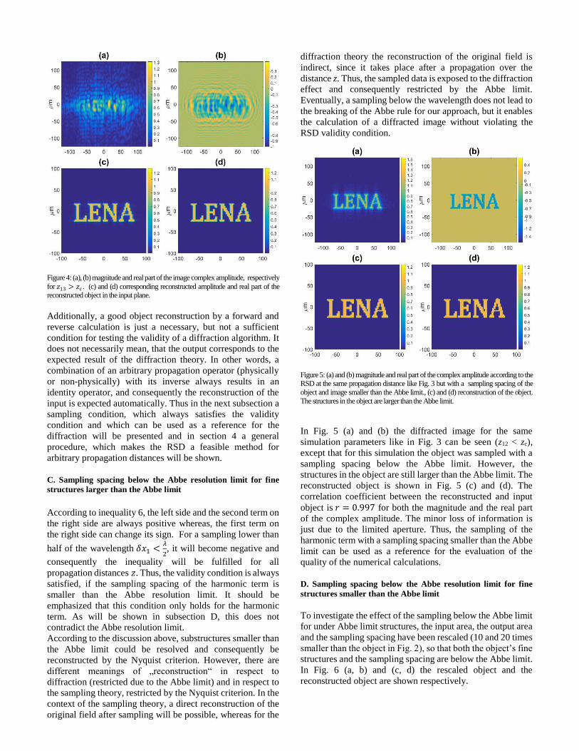
Figure 4: (a), (b) magnitude and real part of the image complex amplitude, respectively

for 𝑧13 > 𝑧𝑐 . (c) and (d) corresponding reconstructed amplitude and real part of the reconstructed object in the input plane.

Additionally, a good object reconstruction by a forward and

reverse calculation is just a necessary, but not a sufficient

condition for testing the validity of a diffraction algorithm. It

does not necessarily mean, that the output corresponds to the

expected result of the diffraction theory. In other words, a

combination of an arbitrary propagation operator (physically

or non-physically) with its inverse always results in an

identity operator, and consequently the reconstruction of the

input is expected automatically. Thus in the next subsection a

sampling condition, which always satisfies the validity

condition and which can be used as a reference for the

diffraction will be presented and in section 4 a general

procedure, which makes the RSD a feasible method for

arbitrary propagation distances will be shown.

C. Sampling spacing below the Abbe resolution limit for fine

structures larger than the Abbe limit

According to inequality 6, the left side and the second term on

the right side are always positive whereas, the first term on

the right side can change its sign. For a sampling lower than

half of the wavelength 𝛿𝑥1 <𝜆

2, it will become negative and

consequently the inequality will be fulfilled for all

propagation distances 𝑧. Thus, the validity condition is always

satisfied, if the sampling spacing of the harmonic term is

smaller than the Abbe resolution limit. It should be

emphasized that this condition only holds for the harmonic

term. As will be shown in subsection D, this does not

contradict the Abbe resolution limit.

According to the discussion above, substructures smaller than

the Abbe limit could be resolved and consequently be

reconstructed by the Nyquist criterion. However, there are

different meanings of „reconstruction“ in respect to

diffraction (restricted due to the Abbe limit) and in respect to

the sampling theory, restricted by the Nyquist criterion. In the

context of the sampling theory, a direct reconstruction of the

original field after sampling will be possible, whereas for the

diffraction theory the reconstruction of the original field is

indirect, since it takes place after a propagation over the

distance z. Thus, the sampled data is exposed to the diffraction

effect and consequently restricted by the Abbe limit.

Eventually, a sampling below the wavelength does not lead to

the breaking of the Abbe rule for our approach, but it enables

the calculation of a diffracted image without violating the

RSD validity condition.

Figure 5: (a) and (b) magnitude and real part of the complex amplitude according to the RSD at the same propagation distance like Fig. 3 but with a sampling spacing of the

object and image smaller than the Abbe limit., (c) and (d) reconstruction of the object.

The structures in the object are larger than the Abbe limit.

In Fig. 5 (a) and (b) the diffracted image for the same

simulation parameters like in Fig. 3 can be seen (z12 < zc),

except that for this simulation the object was sampled with a

sampling spacing below the Abbe limit. However, the

structures in the object are still larger than the Abbe limit. The

reconstructed object is shown in Fig. 5 (c) and (d). The

correlation coefficient between the reconstructed and input

object is 𝑟 = 0.997 for both the magnitude and the real part

of the complex amplitude. The minor loss of information is

just due to the limited aperture. Thus, the sampling of the

harmonic term with a sampling spacing smaller than the Abbe

limit can be used as a reference for the evaluation of the

quality of the numerical calculations.

D. Sampling spacing below the Abbe resolution limit for fine

structures smaller than the Abbe limit

To investigate the effect of the sampling below the Abbe limit

for under Abbe limit structures, the input area, the output area

and the sampling spacing have been rescaled (10 and 20 times

smaller than the object in Fig. 2), so that both the object’s fine

structures and the sampling spacing are below the Abbe limit.

In Fig. 6 (a, b) and (c, d) the rescaled object and the

reconstructed object are shown respectively.

Figure 6: (a), (b) magnitude and the real part of the complex amplitude for

the rescaled input object. (c) and (d) magnitude and real part of the complex

amplitude for the reconstructed object for a sampling spacing below the Abbe

limit 𝛿𝑥1 = 𝛿𝑦1 = 0.025 μm <𝜆

2= 0.32 μm.

As can be seen, due to the violation of the Abbe resolution

limit, the fine structures of the object in Fig. 6 cannot be

resolved anymore. The calculated correlation coefficients

are 𝑟 = 0.88 and 𝑟 = 0.89 for the magnitude and the real part

of the complex amplitude respectively.

Figure 7: (a) and (b) magnitude and real part of the complex amplitude of the

input object. (c) and (d) magnitude and real part of the complex amplitude

for the corresponding output by a sampling below the Abbe limit 𝛿𝑥1 =

𝛿𝑦1 = 0.013 𝜇𝑚<<𝜆

2= 0.32 𝜇𝑚.

For a further reduction of the fine structures in the object the

effect is increased as can be seen in Fig. 7 (a-d). The

calculated correlation coefficients are only 𝑟 = 0.62 and 𝑟 =0.63.Thus, a subwavelength sampling in RSD cannot retain

the full object information, if the fine substructures are below

the Abbe limit.

4. General solution for removing the limitation

of the propagation distance

In practical applications the sampling of the object is restricted by a

minimum spacing as a consequence of the limited pixel size of a

given CCD camera. Here a general solution for an arbitrary distance

from the object will be presented.

The RSD is a linear operator ℛ , which transforms an input

field 𝑢1(𝑟 ) over a propagation distance 𝑧12 into the

field 𝑢12 = ℛ12{𝑢1}. Theoretically, for an unlimited aperture

the information in the input plane 𝑢1 is completely conserved

in the diffracted image 𝑢12. Therefore, the field 𝑢1 can be

reconstructed from the field 𝑢12 by a reverse application of

the RSD with 𝑧 → – 𝑧. The combination of the forward

operator ℛ12 and the reverse operator ℛ21 (𝑢1 =ℛ21{𝑢12}) of the field is an identical operator ℛ21ℛ12 = 𝕝 . Thus, it can be written that ℛ21ℛ12{𝑢1} = 𝕝 {𝑢1} =𝑢1 (for 𝑧12 > 𝑧12c

).

If the validity condition is not satisfied 𝑧12 < 𝑧12c, a complete

reconstruction is not possible and ℛ21ℛ12 ≠ 𝕝. If a set Υ of

all propagation distances satisfying the validity condition is

introduced, it follows that the reverse transform is not an

inverse transform if z ∉ Υ. Although analytically the reverse

and the inverse transforms are identical. Thus, a perfect

reconstruction of all the information in the object is only

possible if ℛ21ℛ12 = 𝕝. Therefore an RSD operator, which

satisfies ℛ21ℛ12 = 𝕝 for z ∉ Υ has to be found.

As described in the last section, at the distance 𝑧13 ∈ Υ, the

reconstruction of the object is almost perfect but, outside the

validity condition 𝑧12 ∉ Υ, the whole object information

cannot be retrieved from the field 𝑢12. Thus for a general

solution, the following approach is proposed: in a first step the

image at a longer distance which satisfies the validity

condition and identity relation 𝑧13 ∈ Υ, is calculated with the

additional property 𝑧13 − 𝑧12 ∈ Υ. In a second step a new

propagation distance 𝑧23 = 𝑧13 − 𝑧12 ∈ Υ will be calculated

with ℛ23 = ℛ32−1. The operator ℛ32 transforms the field 𝑢13 at

𝑧13 to the field 𝑢132 at a shorter distance 𝑧12 . Thus, the

operator ℛ132 = ℛ32ℛ13 , which transforms the field 𝑢1 to

the field 𝑢132 = ℛ132{𝑢1} at the distance 𝑧12 is introduced.

Although 𝑧12 ∉ Υ, it can be easily shown that ℛ231 satisfies

the identity relation as follows:

The reverse of the operator ℛ132 is the operator ℛ231.

According to operator theory [16]:

ℛ231ℛ132 = (ℛ31ℛ23) (ℛ32ℛ13) = ℛ31ℛ23ℛ32ℛ13

Which means the reverse and inverse transforms are the

same ℛ231 = ℛ132−1 . If the loss of information due to the

limited aperture for practical applications is neglected, the

new image 𝑢132 contains all information from 𝑢1.

The operator ℛ132 depends on two propagation variables 𝑧12

and 𝑧13. The first is the real variable, which determines the

distance between the object and the image. The second is just

an arbitrary parameter which has to fulfill the condition 𝑧13 ∈

= ℛ13−1ℛ32

−1ℛ32ℛ13 = ℛ13−1𝕝ℛ13 = 𝕝 (11)

Υ, 𝑧13 − 𝑧12 ∈ Υ. Thus, the set Υ has an infinite number of

elements, which are all valid. However, a cutting of diffracted

field values due to the limited size of the computational plane

3 leads to a loss of information. Thus, for a fixed value of the

pixel size and pixel number, the optimal choice for the

propagation distance 𝑧13 is the minimum allowed value. In

Fig. 8 the calculated field 𝑢132 at the distance 𝑧12 ∉ Υ is

compared with the field 𝑢12 at the same distance. This field

𝑢12 was calculated for a sampling spacing below the Abbe

limit and can be used as a reference, as discussed in section

3C.

Figure 8: (a) and (b) magnitude and real part of the complex amplitude 𝑢132 ,

(c) and (d) magnitude and real part of the complex amplitude 𝑢12 by sampling below the Abbe limit, used as a reference.

The correlation coefficient for the magnitude and real part of

the amplitude are 𝑟 = 0.97 respectively 𝑟 = 0.95, which

shows a remarkable improvement compared to 𝑟 = 0.65

and 𝑟 = 0.49 for the case of applying the conventional

RSD ℛ12 . If we compare the image in Fig. 3 (a), (b) with the

below Abbe sampling image in Fig. 8 (c) and (d), we have a

32% improvement in the magnitude and 46% in the real part

of the amplitude.

In Fig. 9 the reconstruction of the object 𝑢13231 by the use of

the operator ℛ132 for the forward and ℛ231 for the backward

propagation is presented. The correlation coefficients for the

magnitude and the real part of the complex amplitude are 𝑟 =0.97. Again the validity and capability of the proposed

approach can be seen.

Figure 9: (a), (b) amplitude and real part of the input object (c), (d) magnitude

and real part of the amplitude for the reconstructed object.

5. Conclusion

In this paper the numerical treatment of the Rayleigh-Sommerfeld

diffraction was investigated in detail. A validity condition for the

numerical calculation was derived. As have been shown, for a fixed

sampling spacing in the computational domain, the allowed

propagation distance is restricted to a minimum value. However, the

restriction can be completely removed if the sampling spacing (not

the structure in the object) is lower than the Abbe limit. As have been

shown, this results in the maximum obtainable information in the

output plane under the consideration of the limited computational

domain, and was therefore used as a reference. Moreover, a very

general approach for the calculation of the output field for arbitrary

propagation distances was presented. This operator is based on a

combination of forward and reverse RSD transforms and leads to

very high correlation coefficients of 𝑟 = 0.97. An about 30%

improvement in the magnitude of the amplitude and about 45% for

the real part confirms the reliability of the new operator. A

comparison of the results of the below Abbe limit sampling with the

results of the composed operator is an additional verification of both

methods and the consistency of the theoretically derived validity

condition for the RSD. The developed approach can be used as a

reference for the testing of high speed algorithms and other methods,

which are based on the approximation of the exact scalar diffraction

theory.

Acknowledgment. We acknowledge the financial support by the Ministry

of Science and Culture of Lower Saxony in the framework of QUANOMET.

We like to thank Ali Dorostkar for very fruitful discussions, Taranom Akbari

for the creation of Fig. 1 and Julia Böke, Okan Özdemir and Stefan Preußler

for their support during the writing of the paper.

REFERENCES

1. Sommerfeld, Lectures on Theoretical Physics (Academic

Press, New York, 1954) pp. 361-373.

2. J. W. Goodman, Introduction to Fourier Optics

(McGraw-Hill, 1996)

3. M. Born and E. Wolf, Principles of Optics (Pergamon

Press, New York, 1999)

4. Y. M. Engelberg, S. Ruschin, "Fast method for physical

optics propagation of high-numerical-aperture beams," J.

Opt. Soc. Am. A 21, 2135(2004).

5. V. Nascov and P. C. Logofatu, "Fast Computation

algorithm for the Rayleigh-Sommerfeld diffraction

formula using a type of scaled convolution," Appl. Opt.

48, 4310 (2009).

6. F. Shen and A. Wang, "Fast-Fourier-transform based

numerical integration method for the Rayleigh-

Sommerfeld diffraction formula," Appl. Opt. 45, 1102

(2006).

7. F. Zhang, G. Pedrini, and W. Osten, "Reconstruction

algorithm for high-numerical-aperture holograms

with diffraction-limited resolution," Opt. Lett. 31,

1633(2006).

8. H. Scheffers, "Vereinfachte Ableitung der Formeln für die

Fraunhoferschen Beugungserscheinungen," Ann. d. Phys.

434, 211 (1942).

9. E. Lalor, "Conditions for the Validity of the Angular

Spectrum of Plane Waves," J. Opt. Soc. Am. 58, 1235

(1968).

10. M. Kyoji, "Shifted angular spectrum method for off-

axis numerical propagation," Opt. Express 18,18453

(2010).

11. A. Ritter, "Modified shifted angular spectrum

method for numerical propagation at reduced spatial

sampling rates," Opt. Express 22, 26265 (2014).

12. T.-C. Poon and J.-P. Liu, Introduction to modern digital

holography with Matlab (Cambridge University Press,

2014)

13. E. Wolf and E. W. Marchand, "Comparison of the

Kirchhoff and the Rayleigh–Sommerfeld Theories of

Diffraction at an Aperture," J. Opt. Soc. Am. 54, 587

(1964).

14. R. J. Marks, The Joy of fourier, Analysis, Sampling

Theory, Systems, Multidimensions, Stochastic, Processes,

Random Variables, Signal Recovery, POCS, Time,

Scales, & Applications (Baylor University, 2006).

15. M. W. Farn and J. W. Goodman, "Comparison of

Rayleigh-Sommerfeld and Fresnel solutions for axial

points," J. Opt. Soc. Am. A 7, 948 (1990).

16. E. Kreyszig, Introductory functional analysis with

applications (John Wiley & Sons, 1989).