hal-

0016

7711

, ver

sion

1 -

22

Aug

200

7

Fine frequency shift of single vortex entrance and exit in

superconducting loops

Florian R. Onga1, Olivier Bourgeoisa2, Sergey E. Skipetrovb, Jacques Chaussya, Simona

Popac, Jerome Marsc, Jean-Louis Lacoumec

a Institut Neel, CNRS, Laboratoire associe a l’Universite Joseph Fourier, 38042 Grenoble, France

b Laboratoire de Physique et Modelisation des Milieux Condenses, Maison des Magisteres, CNRS and

Universite Joseph Fourier, 38042 Grenoble, France

c Laboratoire des Images et des Signaux, CNRS, Institut National Polytechnique de Grenoble and

Universite Joseph Fourier, Domaine Universitaire, 38402 Saint Martin d’Heres, France

Abstract

The heat capacity Cp of an array of independent aluminum rings has been measured under

an external magnetic field ~H using highly sensitive ac-calorimetry based on a silicon mem-

brane sensor. Each superconducting vortex entrance induces a phase transition and a heat

capacity jump and hence Cp oscillates with ~H . This oscillatory and non-stationary behaviour

measured versus the magnetic field has been studied using the Wigner-Ville distribution (a

time-frequency representation). It is found that the periodicity of the heat capacity oscilla-

tions varies significantly with the magnetic field; the evolution of the period also depends on

the sweeping direction of the field. This can be attributed to a different behavior between

expulsion and penetration of vortices into the rings. A variation of more than 15% of the pe-

riodicity of the heat capacity jumps is observed as the magnetic field is varied. A description

of this phenomenon is given using an analytical solution of the Ginzburg-Landau equations

of superconductivity.

Keywords : mesoscopic superconductivity, giant vortex states, vortex nucleation/expulsion.

PACS : 74.78.Na ; 74.25.Dw ; 74.25.Bt

doi : 10.1016/j.physc.2007.05.050

1email: florian.ong@grenoble.cnrs.fr2email: olivier.bourgeois@grenoble.cnrs.fr

1

hal-0

0167

711,

ver

sion

1 -

22 A

ug 2

007

Author manuscript, published in "Physica C: Superconductivity and its Applications 466, 1-2 (2007) 37-45" DOI : 10.1016/j.physc.2007.05.050

1 Introduction

Thanks to recent evolutions in micro and nanofabrication processes, new devices are emerging which

permit the study of the specific heat of mesoscopic systems even for samples having very small mass (typ-

ically under 100 nanogram)[1, 2, 3, 4, 5, 6]. This kind of innovative sensor opens up a great possibility of

studies which can be carried out on nanosystems. It enables the study of the phase diagram and the phase

transitions specific to systems of small size. Indeed, the reduction of the dimensions of superconducting

or magnetic systems leads to the appearance of new phase transitions [7], or mechanisms proper to quan-

tum physics which can be studied from a thermal point of view [8, 9, 10]. More specifically, the study of

vortex matter in nano-engineered arrays of mesoscopic superconducting systems is of particular interest.

The effect of the geometry, the thickness of the film or the size of the system compared to a physical

characteristic length scale can be studied from a thermal point of view in order to better understand the

physics of vortex in extreme or particular conditions. In general calorimetry has the advantage of being

sensitive to any energy level in the system. Magnetization for instance is sensitive only to the magnetic

aspect of the sample. Through calorimetric measurements any phase transition whatever its origin is

expected to exhibit a signature.

In a superconducting ring a supercurrent appears to screen or enhance a perpendicular external

magnetic field (described by a vector potential ~A), so as the fluxoid φ′ is fixed to an integer multiple of

φ0 = h/2e (the superconducting quantum flux); φ′ is then given by:

φ′ =

∮[

m∗

e∗~vs + ~A

]

· d~l =

∮[

m∗

e∗~vs

]

· d~l + φ = nφ0 (1)

where m∗, e∗ and ~vs are respectively the mass, the charge and the velocity of the supercurrent carriers,

φ is the magnetic flux threading the integration contour and n is an integer. The integer number n of

fluxoid quanta in the ring is a good quantum number and can be seen as the number of vortices threading

the ring, each vortex carrying a fluxoid quantum φ0. If this kind of systems has been widely studied

theoretically [11, 12] and experimentally [13] from an electrical point of view [15, 14], by magnetic deco-

ration [16] or through magnetization measurements [17, 18], little is known about the thermal behaviour

of superconducting mesoscopic loops[4, 5, 19, 20, 21]. Here we report highly sensitive heat capacity mea-

surements performed on an array of independent mesoscopic superconducting rings of size comparable to

the superconducting coherence length ξ(T ) under an applied magnetic field.

In a previous paper (see Ref.[4]), we have already demonstrated that multiple phase transitions be-

tween states with different vorticities are accompagnied by discontinuities of the heat capacity. Each

vortex entrance (or expulsion) is associated to a mesoscopic phase transition from the n to the n + 1

(or n − 1) state, and as the magnetic field is increased, an oscillating heat capacity is measured with

a periodicity corresponding to a flux quantum φ0 threading a loop. Under specific conditions (lowest

temperatures, zero field cooling) it was also shown that several vortices could enter or exit the loop at

the same time, leading to oscillations of the heat capacity with a periodicity of 2φ0 at 0.85 K and 3φ0

at 0.70 K. An important feature distinguishing this article from Ref. [4] is that here we focus only on

2

hal-0

0167

711,

ver

sion

1 -

22 A

ug 2

007

the 1φ0 periodic oscillations of the heat capacity: even at lowest temperatures the system is prepared

to have only a 1φ0 periodic component. Indeed as it was already mentionned in Ref.[4], the magnetic

history of the loops is very important and determines the way the sample behaves. If the magnetic field

is swept from -40 mT down to zero even at 0.6 K the modulation of the heat capacity is φ0 periodic.

The 3φ0 periodic signal as shown in Ref.[4] is evidenced only when the loops are cooled in zero field

before the magnetic field is swept from zero to a high value of H. This hysteresis of the heat capacity of

mesoscopic sample has been observed on many different situations; this behaviour will be discussed in a

forthcoming paper. Here we avoid the appearance of 2φ0 and 3φ0 periodic oscillations, in order to study

the fine evolution of the periodicity of the heat capacity jumps with regard to the varying magnetic field

and to its sweeping direction. The advantages of working at low temperature are the enhancement of the

signal-to-noise ratio and the increase of the total number of vortices a loop can host. We stress here that

in Ref.[4] we studied the temperature and magnetic field ranges enabling the appearance of multiquanta

transitions. It was shown that the pseudoperiod of the heat capacity versus magnetic flux C(H) can take

discrete values n× φ0. In the present paper we focus on the 1φ0 regime and show that the pseudoperiod

of C(H) is continuously changing as H is swept.

2 Experimental results and analysis

2.1 Heat capacity measurements

The sample studied in this work is composed of an array of N = 4.5 × 105 identical non interacting

superconducting aluminum square loops (see the inset of Fig. 2: each loop has 2 µm side, w = 230 nm

arm width, d = 40 nm thickness, for a total mass m = 80 ng of aluminum). The separation of neighboring

loops is 2 µm. The inter-loop interaction is neglected; we indeed do not expect it to affect our results

significantly because for our sample the mutual inductance (≃ −20 fH) is much smaller than the self

inductance (≃ 5 pH). Thus the mutual magnetic flux always remains much smaller than φ0, and the

energy of magnetic interaction between loops is much smaller than the free energy of a single loop. We

will consider in the following that all the thermal signals are additive, hence the measured heat capacity

is N times the heat capacity of a single loop.

The N mesoscopic square loops are patterned by electron beam lithography on a home-made specific

heat sensor and aluminum is deposited by thermal evaporation. The sensor [2, 4] is composed of a large (4

mm×4 mm) and very thin (5 µm) silicon membrane suspended by twelve silicon arms. On this membrane,

a copper heater and a NbN thermometer are deposited through regular photolithography. Resistances of

these thin film transducers are measured by a four point probe technique. In the case of the Cu heater

we can thus measure the power injected in the calorimeter. In the case of the thermometer the four wire

measurement reduces the measuring noise, enabling the read out of very small temperature variations

on which our specific heat measurement is based. Indeed using this device the total heat capacity can

be measured by ac-calorimetry [22]. The principle of this technique lies in applying a sinusoidal current

in the heater at the frequency f , resulting in oscillations of the temperature of the membrane at twice

3

hal-0

0167

711,

ver

sion

1 -

22 A

ug 2

007

this frequency. Thus, when measuring the voltage response on the dc-biased thermometer one gets the

amplitude δTac of the oscillations of the temperature and hence information about the thermal properties

(thermal conductivity and heat capacity) of the silicon membrane and the nanosystems it contains. This

method has been largely described in numerous publications [4, 22, 1, 2]. The calorimetry setup is cooled

down to 0.55 K using a 3He cryostat.

The correct working frequency is obtained by measuring the response function f × δTac of the sensor.

When this response is extremal, i.e. becomes independent of the frequency f , the system can be considered

as quasiadiabatic and then δTac is only related to the heat capacity and to known parameters (frequency

f and injected power) [22]. We define the adiabatic plateau as the frequencies interval such as f × δTac is

greater than 99% of its maximum. In our case we obtain f ∈ [108; 149 Hz] at 0.6 K; in these conditions

the thermal excitation is faster than the characteristic time of the heat loss to the thermal bath but slower

than the heat diffusion time in the system (sensor and sample). The major advantage of working with

lithographied loops is the high thermal contact between the nano-objects and the silicon sensor. In this

quasiadiabatic limit, all superconducting loops can be considered as being at the same temperature. The

amplitude δTac of the oscillations of temperature can be tuned between 1 mK to 15 mK depending on

the working temperature and on the resolution needed for the measurements. The ac-calorimetry enables

averaging of the measured signal, thus reducing the error bar for each measured data point. Typically by

averaging over 10 seconds, this apparatus allows measurements of heat capacity within 10 femto-Joule

per Kelvin, which corresponds to an energy sensitivity as small as few atto-Joule (10−18 Joule).

The sensor is placed in the center of a large superconducting coil so that a tunable magnetic field ~H

can be applied perpendicular to the plane of the loops. The area containing the loops is 2.5 mm×2.8

mm large, and the difference between the field on the axis and the field at the border of the sample has

been calculated to be less than 0.1%. This is regarded as negligible and hence the field is considered as

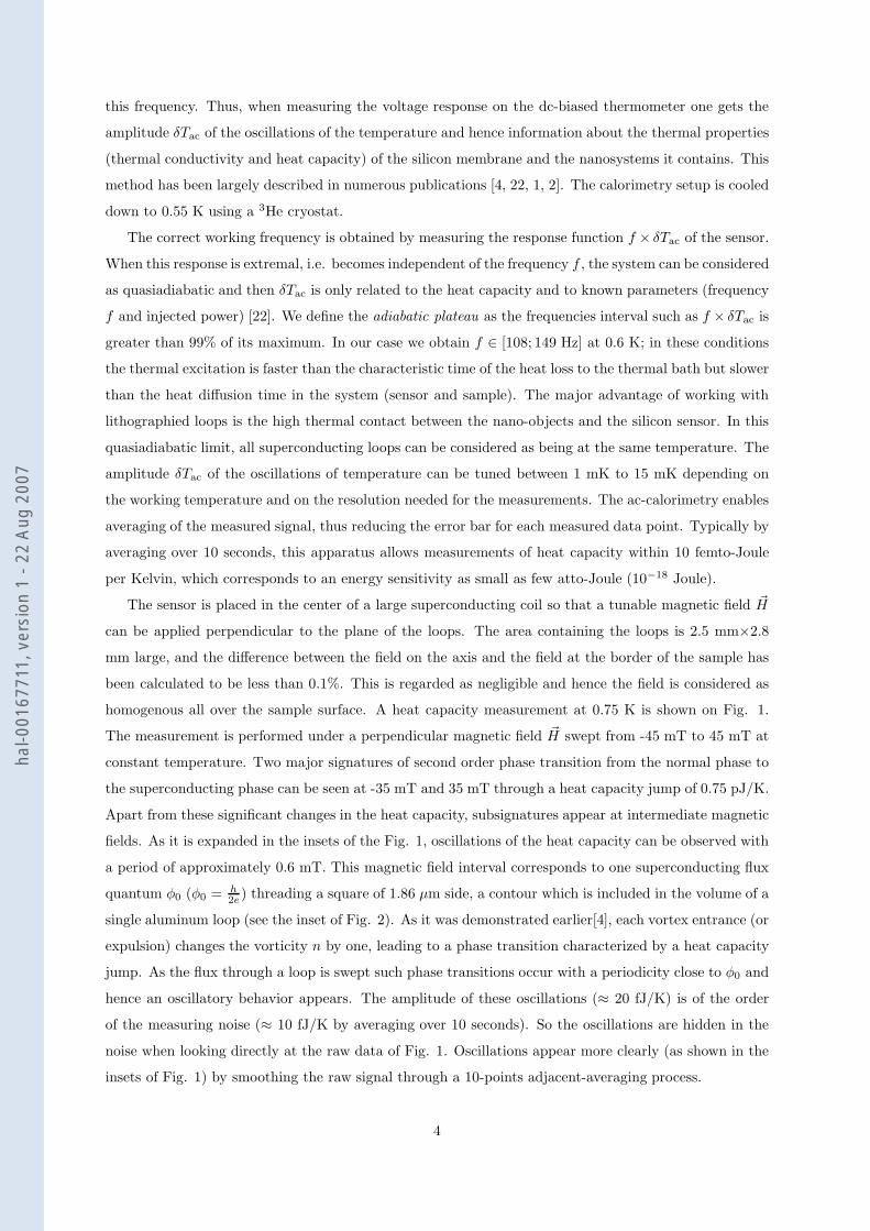
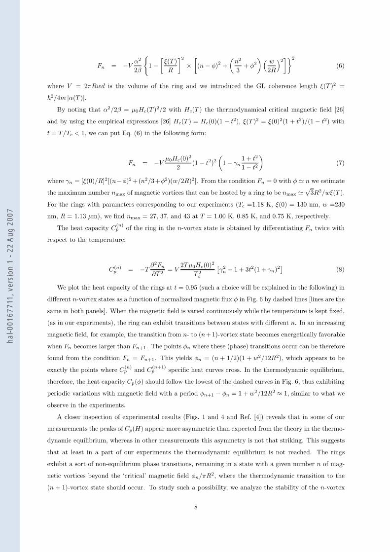
homogenous all over the sample surface. A heat capacity measurement at 0.75 K is shown on Fig. 1.

The measurement is performed under a perpendicular magnetic field ~H swept from -45 mT to 45 mT at

constant temperature. Two major signatures of second order phase transition from the normal phase to

the superconducting phase can be seen at -35 mT and 35 mT through a heat capacity jump of 0.75 pJ/K.

Apart from these significant changes in the heat capacity, subsignatures appear at intermediate magnetic

fields. As it is expanded in the insets of the Fig. 1, oscillations of the heat capacity can be observed with

a period of approximately 0.6 mT. This magnetic field interval corresponds to one superconducting flux

quantum φ0 (φ0 = h2e) threading a square of 1.86 µm side, a contour which is included in the volume of a

single aluminum loop (see the inset of Fig. 2). As it was demonstrated earlier[4], each vortex entrance (or

expulsion) changes the vorticity n by one, leading to a phase transition characterized by a heat capacity

jump. As the flux through a loop is swept such phase transitions occur with a periodicity close to φ0 and

hence an oscillatory behavior appears. The amplitude of these oscillations (≈ 20 fJ/K) is of the order

of the measuring noise (≈ 10 fJ/K by averaging over 10 seconds). So the oscillations are hidden in the

noise when looking directly at the raw data of Fig. 1. Oscillations appear more clearly (as shown in the

insets of Fig. 1) by smoothing the raw signal through a 10-points adjacent-averaging process.

4

hal-0

0167

711,

ver

sion

1 -

22 A

ug 2

007

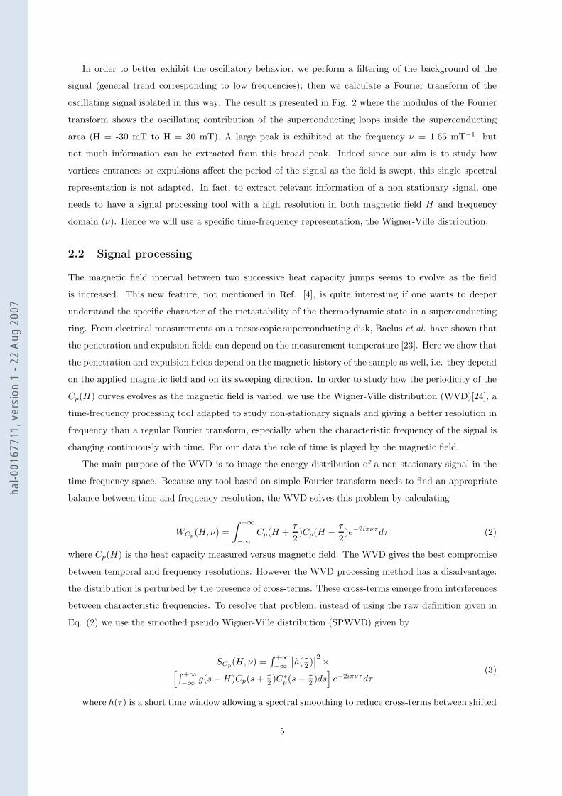
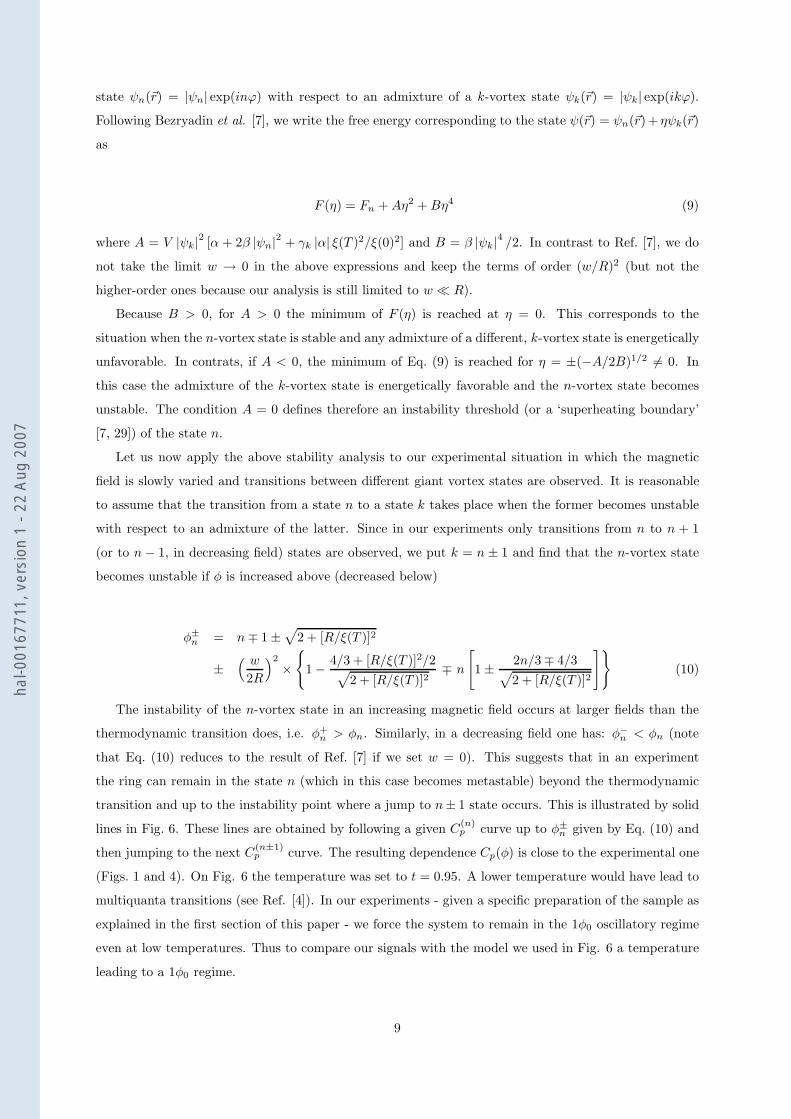
In order to better exhibit the oscillatory behavior, we perform a filtering of the background of the

signal (general trend corresponding to low frequencies); then we calculate a Fourier transform of the

oscillating signal isolated in this way. The result is presented in Fig. 2 where the modulus of the Fourier

transform shows the oscillating contribution of the superconducting loops inside the superconducting

area (H = -30 mT to H = 30 mT). A large peak is exhibited at the frequency ν = 1.65 mT−1, but

not much information can be extracted from this broad peak. Indeed since our aim is to study how

vortices entrances or expulsions affect the period of the signal as the field is swept, this single spectral

representation is not adapted. In fact, to extract relevant information of a non stationary signal, one

needs to have a signal processing tool with a high resolution in both magnetic field H and frequency

domain (ν). Hence we will use a specific time-frequency representation, the Wigner-Ville distribution.

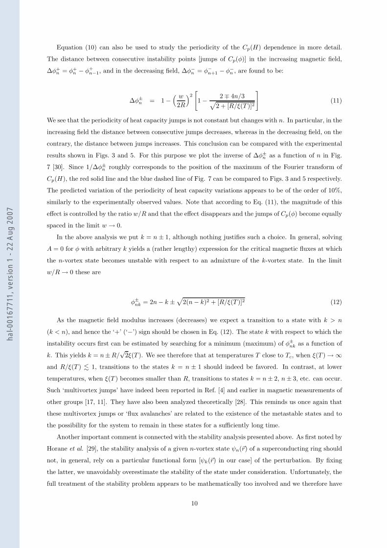
2.2 Signal processing

The magnetic field interval between two successive heat capacity jumps seems to evolve as the field

is increased. This new feature, not mentioned in Ref. [4], is quite interesting if one wants to deeper

understand the specific character of the metastability of the thermodynamic state in a superconducting

ring. From electrical measurements on a mesoscopic superconducting disk, Baelus et al. have shown that

the penetration and expulsion fields can depend on the measurement temperature [23]. Here we show that

the penetration and expulsion fields depend on the magnetic history of the sample as well, i.e. they depend

on the applied magnetic field and on its sweeping direction. In order to study how the periodicity of the

Cp(H) curves evolves as the magnetic field is varied, we use the Wigner-Ville distribution (WVD)[24], a

time-frequency processing tool adapted to study non-stationary signals and giving a better resolution in

frequency than a regular Fourier transform, especially when the characteristic frequency of the signal is

changing continuously with time. For our data the role of time is played by the magnetic field.

The main purpose of the WVD is to image the energy distribution of a non-stationary signal in the

time-frequency space. Because any tool based on simple Fourier transform needs to find an appropriate

balance between time and frequency resolution, the WVD solves this problem by calculating

WCp(H, ν) =

∫ +∞

−∞

Cp(H +τ

2)Cp(H − τ

2)e−2iπντdτ (2)

where Cp(H) is the heat capacity measured versus magnetic field. The WVD gives the best compromise

between temporal and frequency resolutions. However the WVD processing method has a disadvantage:

the distribution is perturbed by the presence of cross-terms. These cross-terms emerge from interferences

between characteristic frequencies. To resolve that problem, instead of using the raw definition given in

Eq. (2) we use the smoothed pseudo Wigner-Ville distribution (SPWVD) given by

SCp(H, ν) =

∫ +∞

−∞

∣

∣h( τ2 )

∣

∣

2 ×[

∫ +∞

−∞g(s−H)Cp(s+ τ

2 )C∗p (s− τ

2 )ds]

e−2iπντdτ(3)

where h(τ) is a short time window allowing a spectral smoothing to reduce cross-terms between shifted

5

hal-0

0167

711,

ver

sion

1 -

22 A

ug 2

007

time terms and g(s−H) is a frequency window allowing a time smoothing to reduce cross-terms between

shifted frequency terms. Several kinds of windows can be used (see Ref. [25]). In the same way as in

classical spectral analysis, boxcar window function are prohibited, so we use in this work smoothing in

time and frequency through Hanning windows [25]. By applying two Hanning windows (h and g) one

gets the same result as a 2D convolution of the WVD by a 2D window. Consequently SPWVD causes

a slight loss of resolution for the characteristic frequency but enables a strong attenuation of the cross

terms.

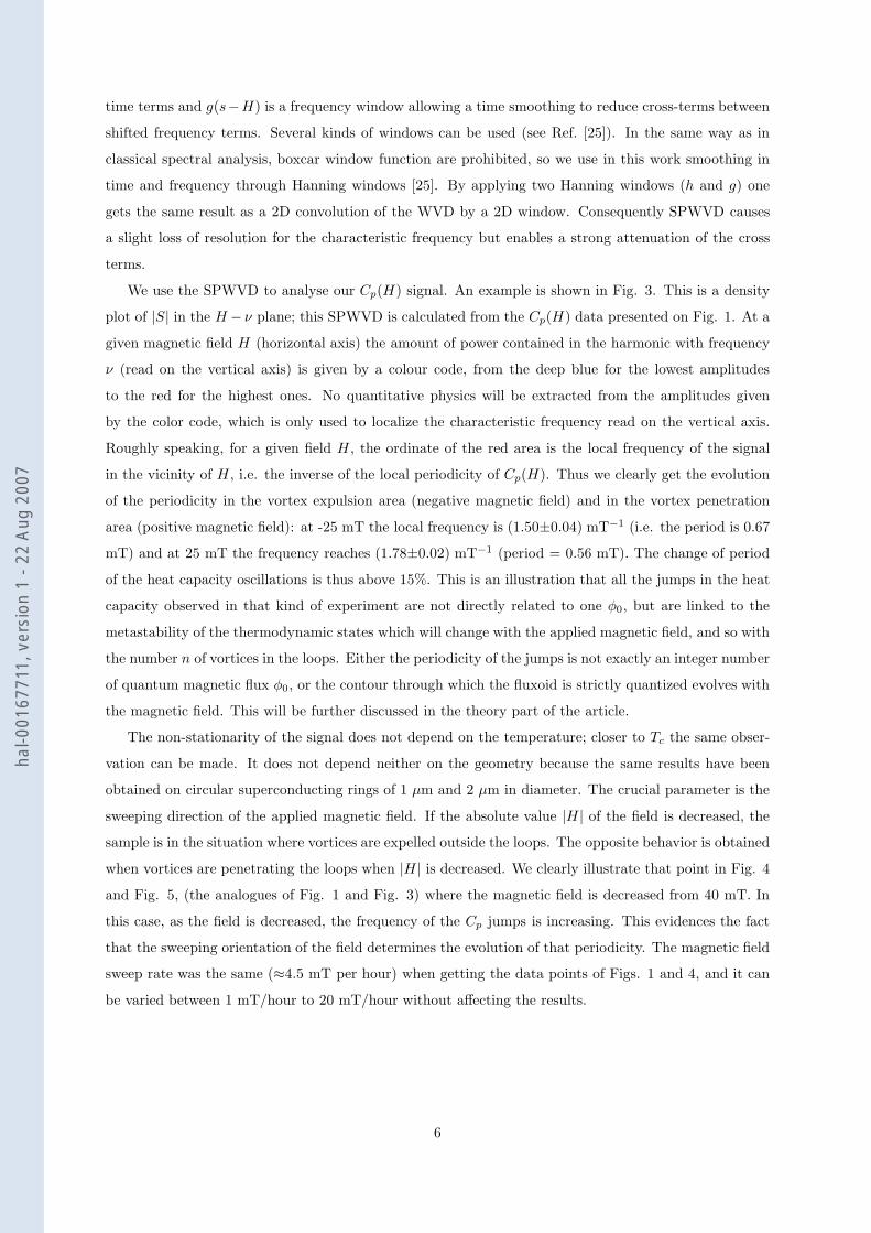
We use the SPWVD to analyse our Cp(H) signal. An example is shown in Fig. 3. This is a density

plot of |S| in the H − ν plane; this SPWVD is calculated from the Cp(H) data presented on Fig. 1. At a

given magnetic field H (horizontal axis) the amount of power contained in the harmonic with frequency

ν (read on the vertical axis) is given by a colour code, from the deep blue for the lowest amplitudes

to the red for the highest ones. No quantitative physics will be extracted from the amplitudes given

by the color code, which is only used to localize the characteristic frequency read on the vertical axis.

Roughly speaking, for a given field H , the ordinate of the red area is the local frequency of the signal

in the vicinity of H , i.e. the inverse of the local periodicity of Cp(H). Thus we clearly get the evolution

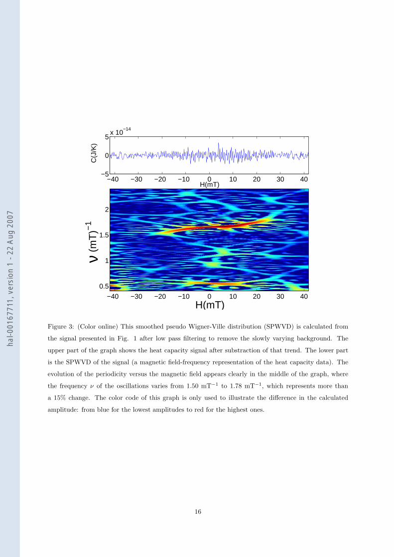
of the periodicity in the vortex expulsion area (negative magnetic field) and in the vortex penetration

area (positive magnetic field): at -25 mT the local frequency is (1.50±0.04) mT−1 (i.e. the period is 0.67

mT) and at 25 mT the frequency reaches (1.78±0.02) mT−1 (period = 0.56 mT). The change of period

of the heat capacity oscillations is thus above 15%. This is an illustration that all the jumps in the heat

capacity observed in that kind of experiment are not directly related to one φ0, but are linked to the

metastability of the thermodynamic states which will change with the applied magnetic field, and so with

the number n of vortices in the loops. Either the periodicity of the jumps is not exactly an integer number

of quantum magnetic flux φ0, or the contour through which the fluxoid is strictly quantized evolves with

the magnetic field. This will be further discussed in the theory part of the article.

The non-stationarity of the signal does not depend on the temperature; closer to Tc the same obser-

vation can be made. It does not depend neither on the geometry because the same results have been

obtained on circular superconducting rings of 1 µm and 2 µm in diameter. The crucial parameter is the

sweeping direction of the applied magnetic field. If the absolute value |H | of the field is decreased, the

sample is in the situation where vortices are expelled outside the loops. The opposite behavior is obtained

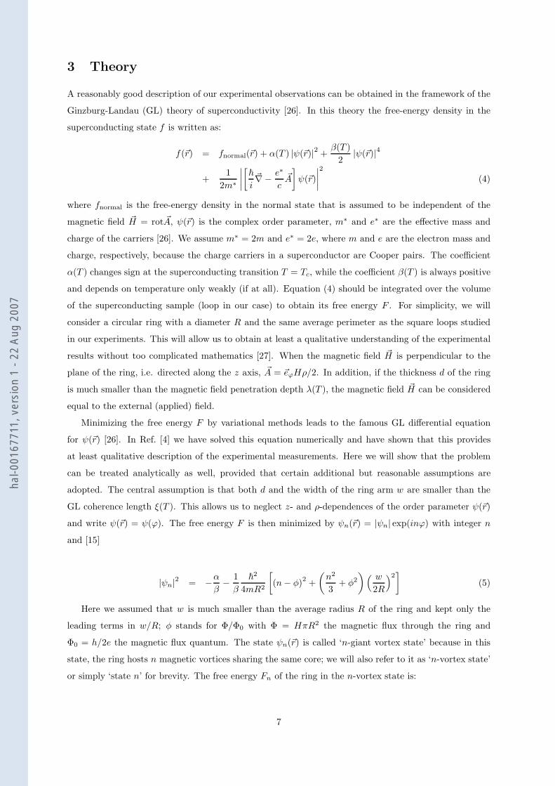
when vortices are penetrating the loops when |H | is decreased. We clearly illustrate that point in Fig. 4

and Fig. 5, (the analogues of Fig. 1 and Fig. 3) where the magnetic field is decreased from 40 mT. In

this case, as the field is decreased, the frequency of the Cp jumps is increasing. This evidences the fact

that the sweeping orientation of the field determines the evolution of that periodicity. The magnetic field

sweep rate was the same (≈4.5 mT per hour) when getting the data points of Figs. 1 and 4, and it can

be varied between 1 mT/hour to 20 mT/hour without affecting the results.

6

hal-0

0167

711,

ver

sion

1 -

22 A

ug 2

007

3 Theory

A reasonably good description of our experimental observations can be obtained in the framework of the

Ginzburg-Landau (GL) theory of superconductivity [26]. In this theory the free-energy density in the

superconducting state f is written as:

f(~r) = fnormal(~r) + α(T ) |ψ(~r)|2 +β(T )

2|ψ(~r)|4

+1

2m∗

∣

∣

∣

∣

[

~

i~∇− e∗

c~A

]

ψ(~r)

∣

∣

∣

∣

2

(4)

where fnormal is the free-energy density in the normal state that is assumed to be independent of the

magnetic field ~H = rot ~A, ψ(~r) is the complex order parameter, m∗ and e∗ are the effective mass and

charge of the carriers [26]. We assume m∗ = 2m and e∗ = 2e, where m and e are the electron mass and

charge, respectively, because the charge carriers in a superconductor are Cooper pairs. The coefficient

α(T ) changes sign at the superconducting transition T = Tc, while the coefficient β(T ) is always positive

and depends on temperature only weakly (if at all). Equation (4) should be integrated over the volume

of the superconducting sample (loop in our case) to obtain its free energy F . For simplicity, we will

consider a circular ring with a diameter R and the same average perimeter as the square loops studied

in our experiments. This will allow us to obtain at least a qualitative understanding of the experimental

results without too complicated mathematics [27]. When the magnetic field ~H is perpendicular to the

plane of the ring, i.e. directed along the z axis, ~A = ~eϕHρ/2. In addition, if the thickness d of the ring

is much smaller than the magnetic field penetration depth λ(T ), the magnetic field ~H can be considered

equal to the external (applied) field.

Minimizing the free energy F by variational methods leads to the famous GL differential equation

for ψ(~r) [26]. In Ref. [4] we have solved this equation numerically and have shown that this provides

at least qualitative description of the experimental measurements. Here we will show that the problem

can be treated analytically as well, provided that certain additional but reasonable assumptions are

adopted. The central assumption is that both d and the width of the ring arm w are smaller than the

GL coherence length ξ(T ). This allows us to neglect z- and ρ-dependences of the order parameter ψ(~r)

and write ψ(~r) = ψ(ϕ). The free energy F is then minimized by ψn(~r) = |ψn| exp(inϕ) with integer n

and [15]

|ψn|2 = −αβ− 1

β

~2

4mR2

[

(n− φ)2 +

(

n2

3+ φ2

)

( w

2R

)2]

(5)

Here we assumed that w is much smaller than the average radius R of the ring and kept only the

leading terms in w/R; φ stands for Φ/Φ0 with Φ = HπR2 the magnetic flux through the ring and

Φ0 = h/2e the magnetic flux quantum. The state ψn(~r) is called ‘n-giant vortex state’ because in this

state, the ring hosts n magnetic vortices sharing the same core; we will also refer to it as ‘n-vortex state’

or simply ‘state n’ for brevity. The free energy Fn of the ring in the n-vortex state is:

7

hal-0

0167

711,

ver

sion

1 -

22 A

ug 2

007

Fn = −V α2

2β

{

1 −[

ξ(T )

R

]2

×[

(n− φ)2 +

(

n2

3+ φ2

)

( w

2R

)2]}2

(6)

where V = 2πRwd is the volume of the ring and we introduced the GL coherence length ξ(T )2 =

~2/4m |α(T )|.

By noting that α2/2β = µ0Hc(T )2/2 with Hc(T ) the thermodynamical critical magnetic field [26]

and by using the empirical expressions [26] Hc(T ) = Hc(0)(1 − t2), ξ(T )2 = ξ(0)2(1 + t2)/(1 − t2) with

t = T/Tc < 1, we can put Eq. (6) in the following form:

Fn = −V µ0Hc(0)2

2(1 − t2)2

(

1 − γn1 + t2

1 − t2

)

(7)

where γn = [ξ(0)/R]2[(n−φ)2 +(n2/3+φ2)(w/2R)2]. From the condition Fn = 0 with φ ≃ n we estimate

the maximum number nmax of magnetic vortices that can be hosted by a ring to be nmax ≃√

3R2/wξ(T ).

For the rings with parameters corresponding to our experiments (Tc =1.18 K, ξ(0) = 130 nm, w =230

nm, R = 1.13 µm), we find nmax = 27, 37, and 43 at T = 1.00 K, 0.85 K, and 0.75 K, respectively.

The heat capacity C(n)p of the ring in the n-vortex state is obtained by differentiating Fn twice with

respect to the temperature:

C(n)p = −T ∂

2Fn

∂T 2= V

2Tµ0Hc(0)2

T 2c

[

γ2n − 1 + 3t2(1 + γn)2

]

(8)

We plot the heat capacity of the rings at t = 0.95 (such a choice will be explained in the following) in

different n-vortex states as a function of normalized magnetic flux φ in Fig. 6 by dashed lines [lines are the

same in both panels]. When the magnetic field is varied continuously while the temperature is kept fixed,

(as in our experiments), the ring can exhibit transitions between states with different n. In an increasing

magnetic field, for example, the transition from n- to (n+1)-vortex state becomes energetically favorable

when Fn becomes larger than Fn+1. The points φn where these (phase) transitions occur can be therefore

found from the condition Fn = Fn+1. This yields φn = (n + 1/2)(1 + w2/12R2), which appears to be

exactly the points where C(n)p and C

(n+1)p specific heat curves cross. In the thermodynamic equilibrium,

therefore, the heat capacity Cp(φ) should follow the lowest of the dashed curves in Fig. 6, thus exhibiting

periodic variations with magnetic field with a period φn+1 − φn = 1 + w2/12R2 ≈ 1, similar to what we

observe in the experiments.

A closer inspection of experimental results (Figs. 1 and 4 and Ref. [4]) reveals that in some of our

measurements the peaks of Cp(H) appear more asymmetric than expected from the theory in the thermo-

dynamic equilibrium, whereas in other measurements this asymmetry is not that striking. This suggests

that at least in a part of our experiments the thermodynamic equilibrium is not reached. The rings

exhibit a sort of non-equilibrium phase transitions, remaining in a state with a given number n of mag-

netic vortices beyond the ‘critical’ magnetic field φn/πR2, where the thermodynamic transition to the

(n + 1)-vortex state should occur. To study such a possibility, we analyze the stability of the n-vortex

8

hal-0

0167

711,

ver

sion

1 -

22 A

ug 2

007

state ψn(~r) = |ψn| exp(inϕ) with respect to an admixture of a k-vortex state ψk(~r) = |ψk| exp(ikϕ).

Following Bezryadin et al. [7], we write the free energy corresponding to the state ψ(~r) = ψn(~r)+ ηψk(~r)

as

F (η) = Fn +Aη2 +Bη4 (9)

where A = V |ψk|2 [α + 2β |ψn|2 + γk |α| ξ(T )2/ξ(0)2] and B = β |ψk|4 /2. In contrast to Ref. [7], we do

not take the limit w → 0 in the above expressions and keep the terms of order (w/R)2 (but not the

higher-order ones because our analysis is still limited to w ≪ R).

Because B > 0, for A > 0 the minimum of F (η) is reached at η = 0. This corresponds to the

situation when the n-vortex state is stable and any admixture of a different, k-vortex state is energetically

unfavorable. In contrats, if A < 0, the minimum of Eq. (9) is reached for η = ±(−A/2B)1/2 6= 0. In

this case the admixture of the k-vortex state is energetically favorable and the n-vortex state becomes

unstable. The condition A = 0 defines therefore an instability threshold (or a ‘superheating boundary’

[7, 29]) of the state n.

Let us now apply the above stability analysis to our experimental situation in which the magnetic

field is slowly varied and transitions between different giant vortex states are observed. It is reasonable

to assume that the transition from a state n to a state k takes place when the former becomes unstable

with respect to an admixture of the latter. Since in our experiments only transitions from n to n + 1

(or to n− 1, in decreasing field) states are observed, we put k = n ± 1 and find that the n-vortex state

becomes unstable if φ is increased above (decreased below)

φ±n = n∓ 1 ±√

2 + [R/ξ(T )]2

±( w

2R

)2

×{

1 − 4/3 + [R/ξ(T )]2/2√

2 + [R/ξ(T )]2∓ n

[

1 ± 2n/3 ∓ 4/3√

2 + [R/ξ(T )]2

]}

(10)

The instability of the n-vortex state in an increasing magnetic field occurs at larger fields than the

thermodynamic transition does, i.e. φ+n > φn. Similarly, in a decreasing field one has: φ−n < φn (note

that Eq. (10) reduces to the result of Ref. [7] if we set w = 0). This suggests that in an experiment

the ring can remain in the state n (which in this case becomes metastable) beyond the thermodynamic

transition and up to the instability point where a jump to n± 1 state occurs. This is illustrated by solid

lines in Fig. 6. These lines are obtained by following a given C(n)p curve up to φ±n given by Eq. (10) and

then jumping to the next C(n±1)p curve. The resulting dependence Cp(φ) is close to the experimental one

(Figs. 1 and 4). On Fig. 6 the temperature was set to t = 0.95. A lower temperature would have lead to

multiquanta transitions (see Ref. [4]). In our experiments - given a specific preparation of the sample as

explained in the first section of this paper - we force the system to remain in the 1φ0 oscillatory regime

even at low temperatures. Thus to compare our signals with the model we used in Fig. 6 a temperature

leading to a 1φ0 regime.

9

hal-0

0167

711,

ver

sion

1 -

22 A

ug 2

007

Equation (10) can also be used to study the periodicity of the Cp(H) dependence in more detail.

The distance between consecutive instability points [jumps of Cp(φ)] in the increasing magnetic field,

∆φ+n = φ+

n − φ+n−1, and in the decreasing field, ∆φ−n = φ−n+1 − φ−n , are found to be:

∆φ±n = 1 −( w

2R

)2[

1 − 2 ∓ 4n/3√

2 + [R/ξ(T )]2

]

(11)

We see that the periodicity of heat capacity jumps is not constant but changes with n. In particular, in the

increasing field the distance between consecutive jumps decreases, whereas in the decreasing field, on the

contrary, the distance between jumps increases. This conclusion can be compared with the experimental

results shown in Figs. 3 and 5. For this purpose we plot the inverse of ∆φ±n as a function of n in Fig.

7 [30]. Since 1/∆φ±n roughly corresponds to the position of the maximum of the Fourier transform of

Cp(H), the red solid line and the blue dashed line of Fig. 7 can be compared to Figs. 3 and 5 respectively.

The predicted variation of the periodicity of heat capacity variations appears to be of the order of 10%,

similarly to the experimentally observed values. Note that according to Eq. (11), the magnitude of this

effect is controlled by the ratio w/R and that the effect disappears and the jumps of Cp(φ) become equally

spaced in the limit w → 0.

In the above analysis we put k = n ± 1, although nothing justifies such a choice. In general, solving

A = 0 for φ with arbitrary k yields a (rather lengthy) expression for the critical magnetic fluxes at which

the n-vortex state becomes unstable with respect to an admixture of the k-vortex state. In the limit

w/R → 0 these are

φ±nk = 2n− k ±√

2(n− k)2 + [R/ξ(T )]2 (12)

As the magnetic field modulus increases (decreases) we expect a transition to a state with k > n

(k < n), and hence the ‘+’ (‘−’) sign should be chosen in Eq. (12). The state k with respect to which the

instability occurs first can be estimated by searching for a minimum (maximum) of φ±nk as a function of

k. This yields k = n±R/√

2ξ(T ). We see therefore that at temperatures T close to Tc, when ξ(T ) → ∞and R/ξ(T ) . 1, transitions to the states k = n ± 1 should indeed be favored. In contrast, at lower

temperatures, when ξ(T ) becomes smaller than R, transitions to states k = n± 2, n± 3, etc. can occur.

Such ‘multivortex jumps’ have indeed been reported in Ref. [4] and earlier in magnetic measurements of

other groups [17, 11]. They have also been analyzed theoretically [28]. This reminds us once again that

these multivortex jumps or ‘flux avalanches’ are related to the existence of the metastable states and to

the possibility for the system to remain in these states for a sufficiently long time.

Another important comment is connected with the stability analysis presented above. As first noted by

Horane et al. [29], the stability analysis of a given n-vortex state ψn(~r) of a superconducting ring should

not, in general, rely on a particular functional form [ψk(~r) in our case] of the perturbation. By fixing

the latter, we unavoidably overestimate the stability of the state under consideration. Unfortunately, the

full treatment of the stability problem appears to be mathematically too involved and we therefore have

10

hal-0

0167

711,

ver

sion

1 -

22 A

ug 2

007

chosen to present a less general but much more physically transparent analysis here. Such an analysis

still yield qualitatively correct conclusions.

4 Discussion

After the exposition of the experimental results, the data treatment and the development of the theoretical

model describing our system, a deeper discussion of the main results is needed. Through the calculation

of the SPWVD of the heat capacity signal versus magnetic field, it has been shown that the Cp(H)

oscillations are not stationary. The periodicity of the jumps strongly depends on the sweeping direction

of the magnetic field (increasing or decreasing). From Fig. 3 and Fig. 5, it is clear that when magnetic

vortices are expelled from the loops (by decreasing the absolute value of the magnetic field), the heat

capacity jumps are far from each other, giving a low-frequency oscillation of Cp(H). On the other hand,

when the magnetic field is increased, vortices penetrate the loops and the jumps are closer and closer to

each other, giving high-frequency heat capacity oscillations. This non-stationarity of the heat capacity

oscillations is not negligible because from the experimental data, as well as from the theoretical estimation,

the variation of the periodicity can be greater than 10% between expulsion of the first vortex and the

penetration of the last one.

In other words, and restraining our discussion only to positive magnetic fields, it can be said that as

the field is increased, the system tends to spend less and less time in each successive giant vortex state.

Furthermore when the vorticity n becomes high it appears from Fig. 6 that the occupied states are the

stable ones, in contrast to the low field regime where the system almost always evolves along metastable

states. This means that the higher the vorticity n, the easier it is to add another vortex into the loop,

until the critical field is reached and the superconductivity suppressed. Thus the energy barriers the

systems has to overcome to jump from the n to the n + 1 state tend to disappear at higher fields. In

that last case, the contour through which the fluxoid is quantized is close to the external edge of the

loop and the supercurrents are localized near the outer boundary of the superconductor, leading to the

”traditional” picture of the giant vortex state regarded as a surface superconductivity state [31].

On the other hand, in decreasing field, when the first vortices are expelled out of the loops (high

magnetic field), the successive jumps occur with a large period, meaning that metastable states can

survive for a long time before the energy barrier between the n and n−1 states is suppressed. This feature

is confirmed by Fig. 6: near the critical field the system spends more time in metastable states when

vortices are expelled than it does in increasing field. In this situation the apparent contour through which

the fluxoid is quantized is close to the inner boundary of the loop; the kinetic energy of the supercurrent

carriers is higher than it would be if the system was in its ground state, where the supercurrents are

localized at the outer boundary.

Furthermore the differences between penetration and expulsion of vortices are enhanced due to the

fact that in increasing field the surface barrier can be destroyed by surface defects, which is not the case

in decreasing field [32]. This effect has not been taken into account in the theoritical work leading to Eq.

11

hal-0

0167

711,

ver

sion

1 -

22 A

ug 2

007

11, but it is in good agreement with the small deviation of the experimental data presented in Fig. 3

from the linear behavior predicted by Eq. 11 and Fig. 7.

5 Conclusions

We have studied the heat capacity behavior of an assembly of non-interacting superconducting loops in

applied magnetic field. Heat capacity discontinuities are observed when the magnetic field is swept. The

jumps are associated to vortex expulsion or vortex entrance in the loops. We have studied the variation

of the periodicity of the heat capacity jumps versus the magnetic field. Using the signal processing tool

based on Wigner-Ville distribution, we were able to image the variation of that periodicity versus the

direction of the magnetic field sweep. As the field is increased, the vortices entering the loops are not

submitted to the same barrier of energy as when the field is decreased and the vortices are expelled. The

GL theory describes our experimental observations with reasonable accuracy.

Acknowledgments

We would like to thank E. Andre, P. Lachkar, J-L. Garden, C. Lemonias, B. Fernandez, T. Crozes for

technical support, P. Brosse-Maron, T. Fournier, Ph. Gandit and J. Richard for fruitfull discussions and

help. We thank the Region Rhone-Alpes and the IPMC (Institut de Physique de la Matiere Condensee)

of Grenoble for financing a part of this project.

References

[1] O. Riou, P. Gandit, M. Charalambous, and J. Chaussy, Rev. Sci. Instrum. 68, 1501 (1997).

[2] F. Fominaya, T. Fournier, P. Gandit, and J. Chaussy, Rev. Sci. Instrum. 68, 4191 (1997).

[3] A. Lindell, J. Mattila, P.S. Deo, M. Manninen and J. Pekola Physica B 284, 1884 (2000).

[4] O. Bourgeois, S.E. Skipetrov, F. Ong, and J. Chaussy Phys. Rev. Lett. 94, 057007 (2005).

[5] F.R. Ong, O. Bourgeois, S.E. Skipetrov, and J. Chaussy Phys. Rev. B 74, 140503(R) (2006).

[6] W. Chung Fon, K.C. Schwab, J.M. Worlock, and M.L. Roukes Nano Lett. 5, 1968 (2005).

[7] A. Bezryadin, A. Buzdin, and B. Pannetier, Phys. Rev. B 51, 3718 (1995).

[8] H.J. Fink and V. Grunfeld Phys. Rev. B 23, 1469 (1981).

[9] A. Buzdin Phys. Rev. B 72, 100501(R) (2005).

[10] P.H. Barsic, O.T. Valls and K. Halterman Cond-Mat 0512285 (2005).

[11] D.Y. Vodolazov, F.M. Peeters, S.V. Dubonos, and A.K. Geim, Phys. Rev. B 67, 054506 (2003).

12

hal-0

0167

711,

ver

sion

1 -

22 A

ug 2

007

[12] B.J. Baelus, F.M. Peeters, and V.A. Schweigert, Phys. Rev. B 63, 144517 (2001).

[13] V.V. Moshchalkov, L. Gielen, C. Strunk, R. Jonckheere, X. Qiu, C. Van Haesendonck and Y.

Bruynseraede Nature 373, 319 (1995).

[14] M. Morelle, V. Bruyndoncx, R. Jonckheere, and V.V. Moshchalkov Phys. Rev. B 64, 064516 (2001).

[15] X. Zhang and J.C. Price, Phys. Rev. B 55, 3128 (1997).

[16] B. Pannetier, A. Bezryadin, and A. Eichenberger, Physica B 222, 253 (1996).

[17] S. Pedersen, G.R. Kofod, J.C. Hollingbery, C.B. Sorensen, and P.E. Lindelof, Phys. Rev. B 64,

104522 (2001).

[18] A.K. Geim, I.V. Grigorieva, S.V. Dubonos, J.G.S. Lok, J.C. Maan, A.E. Filippov, and F.M. Peeters,

Nature 390, 259 (1997).

[19] P. Gandit, J. Chaussy, B. Pannetier, A. Vareille, and A. Tissier EuroPhys. Lett. 3, 623 (1987).

[20] O. Buisson, P. Gandit, R. Rammal, Y.Y. Wang, and B. Pannetier Phys. Lett. A 150, 36 (1990).

[21] P. Singha deo, J.P. Pekola, and M. Manninen EuroPhys. Lett. 5, 649 (2000).

[22] P.F. Sullivan and G. Seidel Phys. Rev. 173, 679 (1968).

[23] B.J. Baelus, A. Kanda, F.M. Peeters, Y. Ootuka, and K. Kadowaki Phys. Rev. B 71, 140502(R)

(2005).

[24] W.J. Mecklenbrauker and F. Hlawatsch , The Wigner Distribution (Elsevier eds, Amsterdam, 1997).

[25] F.J. Harris, Proc. of I.E.E.E. 66, 51 (1978).

[26] M. Tinkham, Introduction to Superconductivity (2nd edition, Dover, 2004).

[27] V.M. Fomin, V.R. Misko, J.T. Devreese, V.V. Moshchalkov, Phys. Rev. B 58, 11703 (1998).

[28] D.Y. Vodolazov and F.M. Peeters, Phys. Rev. B 66, 054537 (2002).

[29] E.M. Horane, J.I. Castro, G.C. Buscaglia, and A. Lopez, Phys. Rev. B 53, 9296 (1996); J.I. Castro

and A. Lopez, Phys. Rev. B 72, 224507 (2005).

[30] We calculate 1/∆φ±n up to second order in (w/2R). This yields the same result as Eq. 1 but with an

opposite sign in front of the second term.

[31] D. Saint-James and P.-G. de Gennes, Phys. Lett. 7, 306 (1963).

[32] C.P. Bean and J.B. Livingston, Phys. Rev. Lett. 12, 14 (1964).

13

hal-0

0167

711,

ver

sion

1 -

22 A

ug 2

007

-40 -30 -20 -10 0 10 20 30 40

44.6

44.8

45.0

45.2

45.4

-20 -19 -18 -17 -1644.79

44.82

44.85

44.88

0 1 2 3 4

44.62

44.64

44.66

44.68

Figure 1: Heat capacity measurement of the superconducting rings at 0.75 K. The heat capacity jumps

at -35 mT and 35 mT corresponds to the transition between the superconducting state and the normal

state. The insets focus on two areas after signal processing reducing the visible noise (10 points adjacent

averaging): small heat capacity oscillations appears to be superimposed on a slowly varying background.

The arrow indicates that in this experiment the field is swept from -45 mT to 45 mT.

14

hal-0

0167

711,

ver

sion

1 -

22 A

ug 2

007

Figure 2: Modulus of the Fourier transform of the signal shown in Fig. 1 windowed from H=-30 mT to

H=30 mT (superconducting part of the plot), after low pass filtering to remove the background. A large

peak appears at the frequency ν = 1.65 mT−1, which corresponds to one magnetic flux quantum in a

square of 1.86 µm side. The inset shows an electron micrograph of one loop : the external side is 2.05

µm and the internal side is 1.65 µm.

15

hal-0

0167

711,

ver

sion

1 -

22 A

ug 2

007

−40 −30 −20 −10 0 10 20 30 40−5

0

5x 10

−14

C(J

/K)

H(mT)

H(mT)

(mT

)−1

−40 −30 −20 −10 0 10 20 30 40

0.5

1

1.5

2

ν

Figure 3: (Color online) This smoothed pseudo Wigner-Ville distribution (SPWVD) is calculated from

the signal presented in Fig. 1 after low pass filtering to remove the slowly varying background. The

upper part of the graph shows the heat capacity signal after substraction of that trend. The lower part

is the SPWVD of the signal (a magnetic field-frequency representation of the heat capacity data). The

evolution of the periodicity versus the magnetic field appears clearly in the middle of the graph, where

the frequency ν of the oscillations varies from 1.50 mT−1 to 1.78 mT−1, which represents more than

a 15% change. The color code of this graph is only used to illustrate the difference in the calculated

amplitude: from blue for the lowest amplitudes to red for the highest ones.

16

hal-0

0167

711,

ver

sion

1 -

22 A

ug 2

007

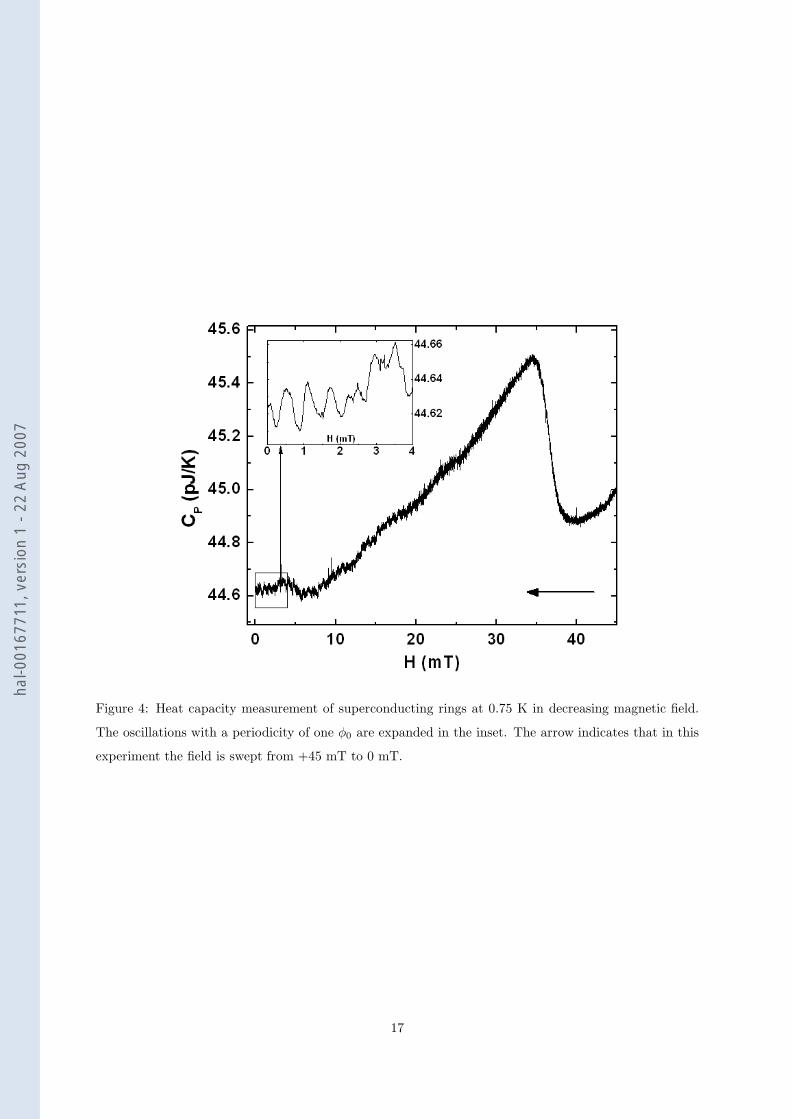
Figure 4: Heat capacity measurement of superconducting rings at 0.75 K in decreasing magnetic field.

The oscillations with a periodicity of one φ0 are expanded in the inset. The arrow indicates that in this

experiment the field is swept from +45 mT to 0 mT.

17

hal-0

0167

711,

ver

sion

1 -

22 A

ug 2

007

0 5 10 15 20 25 30 35 40−5

0

5x 10

−14

C(J

/K)

H(mT)

H(mT)

(mT

)−1

0 10 20 30 400.5

1

1.5

2

ν

Figure 5: (Color online) This SPWVD is calculated from the signal presented in Fig. 4 after low pass

filtering to remove the slowly varying background (upper part of the graph). The lower part is the

SPWVD of that signal. The evolution of frequency versus magnetic field is inverted as compared to the

case where the magnetic field is increased (see Fig. 3). The color code is the same as in Fig. 3.

18

hal-0

0167

711,

ver

sion

1 -

22 A

ug 2

007

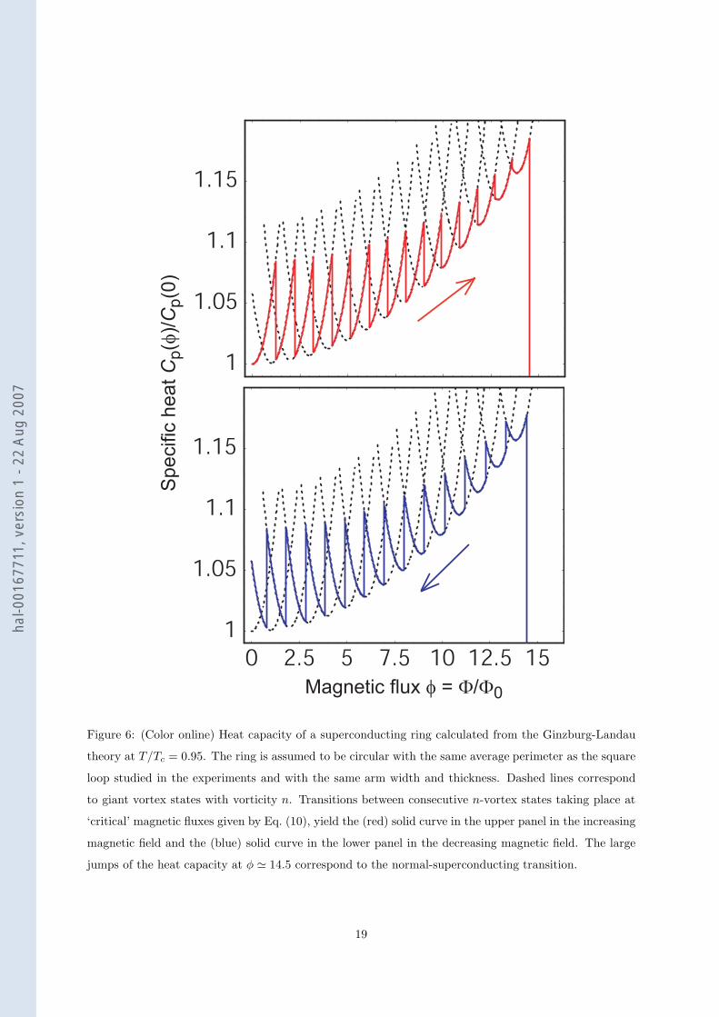
Magnetic flux φ = Φ/Φ0

Specific

heat C

p(φ

)/C

p(0

)

1

1.05

1.1

1.15

0 2.5 5 7.5 10 12.5 15

1

1.05

1.1

1.15

Figure 6: (Color online) Heat capacity of a superconducting ring calculated from the Ginzburg-Landau

theory at T/Tc = 0.95. The ring is assumed to be circular with the same average perimeter as the square

loop studied in the experiments and with the same arm width and thickness. Dashed lines correspond

to giant vortex states with vorticity n. Transitions between consecutive n-vortex states taking place at

‘critical’ magnetic fluxes given by Eq. (10), yield the (red) solid curve in the upper panel in the increasing

magnetic field and the (blue) solid curve in the lower panel in the decreasing magnetic field. The large

jumps of the heat capacity at φ ≃ 14.5 correspond to the normal-superconducting transition.

19

hal-0

0167

711,

ver

sion

1 -

22 A

ug 2

007

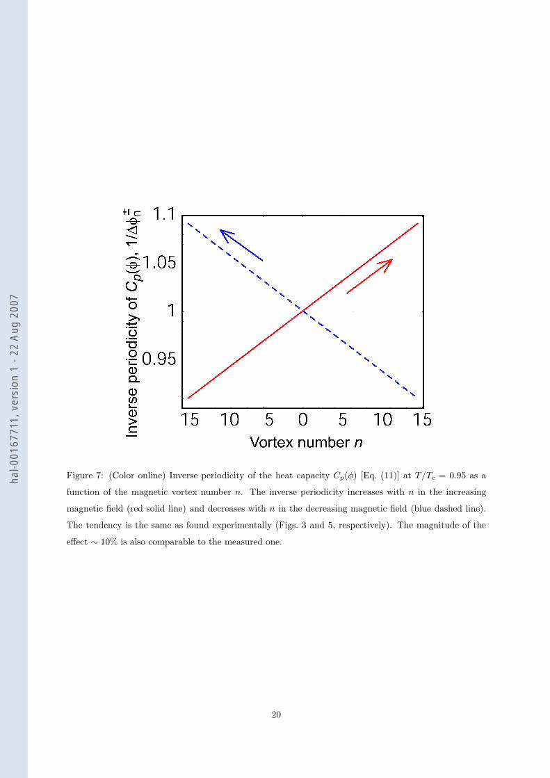
Figure 7: (Color online) Inverse periodicity of the heat capacity Cp(φ) [Eq. (11)] at T/Tc = 0.95 as a

function of the magnetic vortex number n. The inverse periodicity increases with n in the increasing

magnetic field (red solid line) and decreases with n in the decreasing magnetic field (blue dashed line).

The tendency is the same as found experimentally (Figs. 3 and 5, respectively). The magnitude of the

effect ∼ 10% is also comparable to the measured one.

20

hal-0

0167

711,

ver

sion

1 -

22 A

ug 2

007