Finding the Best Viewpoints for Three-Dimensional Graph Drawings

Peter Eades, Michael E. Houle, and Richard Webber

Department of Computer Science and Software Engineering University of Newcastle

Callaghan 2308, Australia {eades, mike, richard}~cs, newcastle, edu. au

Abstract . In this paper we address the problem of finding the best viewpoints for three-dimensional straight-line graph drawings. We define goodness in terms of preserving the relational structure of the graph, and develop two continuous measures of goodness under orthographic parallel projection. We develop Voronoi variants to find the best viewpoints under these measures, and present results on the complexity of these diagrams.

1 I n t r o d u c t i o n

Three-dimensional drawings of graphs are being used in many areas of com- puting. For example: to visualise the structures of object-oriented [16,24] and parallel [22] software; for interactive information retrieval [11]; and to navigate the World-Wide Web [18,20].

There has been much work on creating graph drawings that are both easy to remember and easy to understand [8]. Most work has been to produce two- dimensional drawings, but recent work addresses three-dimensions [6]. Much of this work has concentrated on the problems of finding a good three-dimensional drawing for a graph. In this paper, we consider a problem in the process of rendering a three-dimensional graph drawing as a two-dimensional image: finding a good viewpoint.

There is some experimental evidence that three-dimensional graph drawings have advantages over their two-dimensional counterparts. One claimed advan- tage [23] is that three dimensions allow users to work with larger graphs - the natural three-dimensional actions of rotation and translation allow users to re- solve ambiguities in large graphs while maintaining their overall mental map [9].

Ware et al. [23] consider the problem of finding connections in a three- dimensional graph drawing, with a variety of display and navigation combi- nations. Using a sequence of human experiments, they show that allowing users to navigate around the drawing results in a significant decrease in the error rate, but at the cost of increased decision time. Current navigation methods tend to require users to manually select their desired viewpoints. We conjecture that the increase in decision time is (partly) due to the time taken to manually select good viewpoints.

88

We propose the use of logical viewpoint selection - the users specify the part of tile graph drawing on which the), wish to focus, and the system automatically selects a (locally) good viewpoint. An additional use for logical viewpoint se- lection is when a three-dimensional graph drawing must be rendered as a static two-dimensional image. Using a good viewpoint under these circumstances can be critical, as was evident in last year's graph drawing contest [10].

Some existing systems already support simple versions of logical selection. The application ivview [21] navigates around three-dimensional scenes. It has a logical selection function that allows users to select a surface in the scene being viewed, then it moves the viewpoint to be perpendicular to the surface.

In Sec. 2 we briefly present some background material, and outline previous work specifically on the problem of finding good viewpoints [4,14]. In Sec. 3 we model good viewpoints in terms of the information conveyed by a drawing, then in Sec. 4 we use the techniques described by Bose, Gomez, Ramos and Toussaint [4] to find all bad viewpoints under our model.

In Sec. 5 we develop two new models that provide continuous measures of the goodness of a viewpoint. We introduce Voronoi variants to find all best viewpoints under these measures, and give proofs of their complexity. Finally, in Sec. 6 we outline future research possibilities based on this work.

2 B a c k g r o u n d

A three-dimensional straight-line drawing D : V + ]R 3 of an abstract graph G = (V, E) associates a three-dimensional position (x~, Yi, zi> with each vertex vi E V. We consider a vertex and its position to be synonymous. Each edge eli is drawn as a line-segment ~ between its end-points. A vertex with no incident edges is an isolated vertex. We denote the set of isolated vertices Vo.

The same abstract graph can be represented by many different drawings, and there are many techniques for automatically generating these drawings. For an extensive collection of graph drawing papers refer to the annotated bibliography by" Di Battista et al. [8].

To convert a three-dimensional graph drawing into a two-dimensional image (for rendering onto a computer screen or paper) we use a projection. In computer graphics, the most common projections are parallel, perspective, and fisheye-lens projections. They approximate the way in which people (or fish) see the world around them.

Projections have parameters, the most important being the viewpoint. This has two components: the position of the viewer in three-dimensional space; and the direction that the viewer is facing. These projections map three-dimensional points onto a two-dimensional surface called the projection surface.

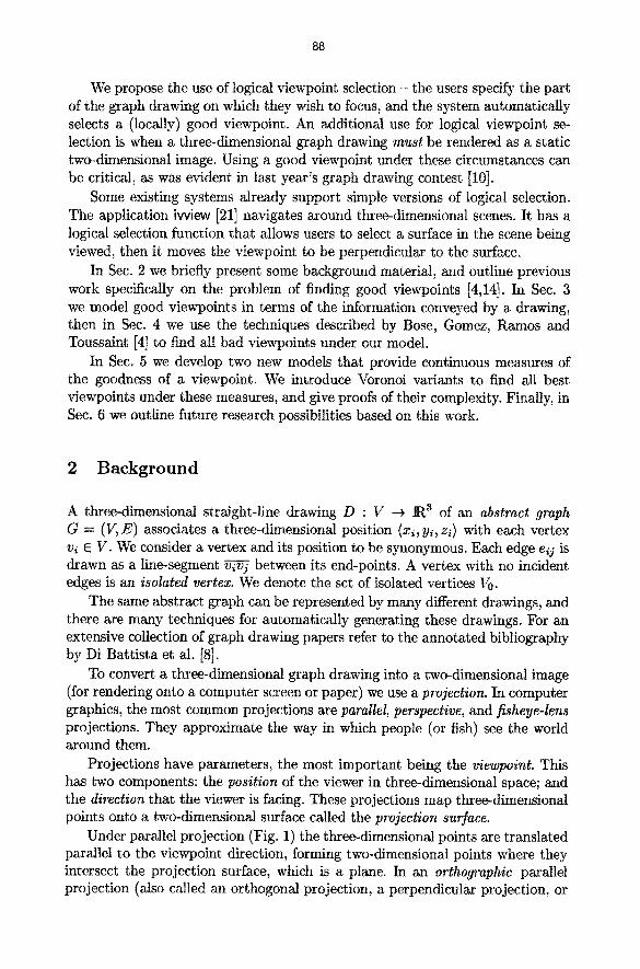
Under parallel projection (Fig. 1) the three-dimensional points are translated parallel to the viewpoint direction, forming two-dimensional points where they intersect the projection surface, which is a plane. In an orthographic parallel projection (also called an orthogonal projection, a perpendicular projection, or

89

proje surfa

viewpoint position

Fig. 1. Orthographic parallel projection.

simply "a projection") the viewpoint direction is perpendicular to the projection surface. A detailed explanation of projections can be found in [12].

If a projection maps two three-dimensional points to the same two-dimensional point, then there is art occlusion. We say the front point (the first one encoun- tered when moving in the viewpoint direction) occludes the rear point.

Both a three-dimensional graph drawing and the two-dimensional result of its projection contain information. The preservation of this information under projection forms the basis for many models of good viewpoints.

Kamada and Kawai [14] model good viewpoints that preserve the shape information of a wire-frame drawing ($~ = 0), excluding viewpoints for which edges appear collinear. Bose et al. [4] preserve the depth-order of a wire-frame drawing, permitting only viewpoints that yield regular projections 1 [17].

In Sec. 3, we define good viewpoints to be those that preserve the abstract graph of a drawing, where a drawing may include isolated vertices. Our definition covers the significant bad viewpoints of Kamada and Kawai, and leads to faster algorithms than those in [4].

Bose et al. suggest an algorithm to describe all bad viewpoints in by building an arrangement [5,19] of curves consisting of bad viewpoints. Under their model this requires O(tEI 3 log IE] + k I) time, where the parameter k' is O(IEI 6) in the worst case. In Sec. 4 we employ the same technique with our simpler model to build an arrangement of bad viewpoints in O(1~ 1 log I~1 + k) time, where I~l = 2(Iv°l) + 21VILE I and k is O(Iko12 ) but can be much less.

Kamada and Kawai use the great-circle distance between a viewpoint and its nearest bad viewpoint as a continuous measure of goodness. We call this rota-

1 A regular projection [17] excludes three three-dimensional points appearing as a single two-dimensional point. The end-points of edges count for two points each.

90

tional separation, and in Sec. 5.1 we show how to find all best viewpoints under rotational separation using the rotational separation diagram. This is a variant of the Voronoi diagram [2] which can be built in O((1~1 + k) log(l~P I + k)) time, with I~1 and k as above. In Sec. 5.2 we define goodness to be the observed separation after projection and describe the observed separation diagram, a Voronoi variant that finds all best viewpoints under observed separation. We also present some results on the complexity of this diagram.

3 Good Viewpoints

Three-dimensional graph drawings are used to convey information. When pro- jecting a drawing into two dimensions we want to preserve this information. This forms the basis for our definition of a good viewpoint.

A three-dimensional graph drawing can convey several forms of information:

- Relational information: the vertices, edges and the incidences between them. - Attribute information: attributes, such as shape and colour, of each element. - Geometric information: the position of each element relative to some known

point (origin), or more typically, the distance between a pair of elements.

Attribute and geometric information are features of a particular drawing of the graph. Attribute information is preserved by most useful projections. Geometric information is highly dependent on the projection and viewpoint used.

Relational information is dependent on the underlying abstract graph. Preser- vation of relational information motivates our definition for a good viewpoint:

Definit ion 1. A good viewpoint is one for which the abstract graphs of the three- dimensional drawing and its two-dimensional projection appear the same.

This in turn depends on how the projection maps each element. For now we make a few simplifying assumptions:

1. We use an orthographic parallel projection. 2. There is no clipping. 3. All vertices and edges are mathematical ideals, with zero width for the pur-

pose of calculating occlusions.

Under an orthographic parallel projection we can parameterise a viewpoint by its normalised direction vector d E $~, where $2 is the unit sphere centred at the origin in ]R 3.

The abstract graphs of a three-dimensional drawing and its two-dimensional projection appear the same under an orthographic parallel projection if and only if there are no occlusions between elements of the drawing. For two graph elements a and b we denote the set of viewpoints that generate occlusions of b by a (a is in front) by ¢(a, b). We refer to the corresponding viewpoints as bad viewpoints.

91

4 d 4 d d d d # # # # # # #

, '- W-7~'- 3'- 3"-7 L -X - . . / - - - #.. - x - - . J

# / l / # # # # # / # # #

1 - - - T - - " / - - - - / f " - - T - - 7 : 2~

"_," . ' " ,' , t J # I i ~u # # /

/ # l # # # / F--T--7----I----F--T--7

I I I l I I l l I l # l / I

1 T

Fig. 2. Vertex-vertex occlusions.

~)(Vi ~ q

d 4 4 [ d d # # I / l I ¢ I 1

I--T--7----I----F--T--7 1 I # I l # .jr '-~-'

# I I # I # #

L_X_J_ _#-_x_.J

I I I I I l I l I I I I I

l--r-7--~l I---T--~

t i I I 11 I I I I I # l #

¢(v~, v0

¢ ( v . vk )

j k , Vi)

Fig. 3. Vertex-edge/edge-vertex occlusions.

There are four pairings of graph elements that generate occlusions:

Vertex-Vertex Occlusions (Fig. 2): A pair of three-dimensional vertices map to a single two-dimensional vertex. The abstract graph of the projection has a single vertex in place of the original two, and any edges incident to the original vertices now appear incident to the combined vertex. The set ¢(vi, vj) contains one element, the normalised vector from vi to vj which we will denote dij.

Vertex-Edge/Edge- Vertex Occlusions (Fig. 3): A three-dimensional vertex maps to an internal point of a two-dimensional edge. The abstract graph of the pro- jection has two edges in place of the original edge, both incident to the vertex. The difference between vertex-edge and edge-vertex occlusions is simply which element is in front. In this case, ¢(vi, ejk) is the set of direction vectors on the great-circle arc between d/j and dik.

Notice that the set of bad viewpoints for a vertex-edge/edge-vertex occlusion is a superset of the bad viewpoints corresponding to the pair of vertex-vertex occlusions of the vertex and each end-point of the edge:

¢(v. e~k) ~ ¢(v.vD u ¢(v~,vk)

92

¢(~j,v~) ¢(~,,v~)

r r - ' ~ - - t - - r r - 7 ~ ( e l j ~ e ~ ! I I I I l I I

, - , ?_:2 I t I I t - t I r-r-7-w--r-?-7 ~ i t l l t t /

I - I t l

I I I I I

l l t l l l 1 I I I I I I I

Fig. 4. Edge-edge occlusions.

We say that the vertex-edge/edge-vertex occlusion covers the vertex-vertex oc- clusions. If we are already checking for vertex-edge/edge-vertex occlusions then we only need to check for vertex-vertex occlusions between pairs of isolated ver- tices. We call these isolated-vertex occlusions.

Edge-Edge Occlusions (Fig. 4): There are two cases of edge-edge occlusions. Case 1 - a pair of three-dimensional edges map to a pair of two-dimensional edges that cross at a single internal point. With straight-line edges, we can (ideally) trace the paths of these edges, and the abstract graph is not effected.

Case 2, significant edge-edge occlusions - the two-dimensional edges share a continuous sequence of points. This only occurs when the three-dimensional edges are coplanar. The abstract graph of the projection has three edges in place of the original two. Some vertices incident to the original edges become incident to the new edge.

For significant edge-edge occlusions, ¢(eij, ekl) is the union of (and hence covered by) four vertex-edge/edge-vertex occlusions:

¢(~ij, ekl) = ¢(v~, eke) U ¢(vj, eke) U ¢(e~j, vk) U ¢(e~j, vd •

If we are already checking for vertex-edge/edge-vertex occlusions then we do not need to check for edge-edge occlusions.

L e m m a 1. A good viewpoint is one that does not generate any isolated-vertex or vertex-edge/edge-vertex occlusions.

4 Bad Viewpoints

For a given three-dimensional drawing of a graph G = (V,E), we want to find all the bad viewpoints. Bose et al. [4] do this by constructing an arrangement of the sets of bad viewpoints under their model. They require O([EI 3 log IEI + k') time and O(IEt 3 + k') space, where k' is the number of intersections in the

93

arrangement, which is O(IEI 6) in the worst case. We apply the same technique to our model, obtaining a description in asymptotically less time and space.

Notice that, under an orthographic parallel projection with no clipping, the viewpoint directions d and - d yield the same two-dimensional projection. It follows that we only need to build the arrangement for one hemisphere.

An arrangement of bad viewpoints is an arrangement of a set ko of points and great-circle arcs on the unit sphere. We can transform this for one hemisphere to an arrangement of points and line-segments in the plane using a central pro- jection [19]. We can now use a segment intersection algorithm in the plane [5,19] to form the arrangement, which leads us to the following result:

Result 1 (Bad Viewpoint Arrangement [4]). For a given three-dimension- al drawing of a graph G = (V, E), we can build a bad viewpoint arrangement in O(l~o t log Ik~l + k) time; I~1 = 2 (Iyol) + 21VILE l is the number of points and great-

circle arcs in the arrangement; k is the number of intersections between them, which is 0(1~12) in the worst case, but can be much less. The arrangement has o(1 1 + k) size.

5 B e s t V i e w p o i n t s

The bad viewpoint arrangement discussed above only distinguishes between good and bad viewpoints. We would prefer to have a continuous measure for the goodness of a viewpoint. In the following sections we discuss two such measures, and show how to find the best viewpoints for a given drawing.

5.1 Rotational Separation

Let the function 5(p, q) denote the great-circle distance between the points p and q on the unit sphere $2. The value of 5(p, q) is also the angle between the vector representations of p and q. We will use either interpretation as appropriate.

We will overload the notation by letting 5(d, ¢(a, b)) denote the minimum great-circle distance (angle) between d and the points (vectors) from the set ¢(a,b). For a vertex-vertex occlusion ¢(v~,vj) this is simply the great-circle distance between d and d~j. For a vertex-edge occlusion ¢(vi, ejk) and an edge- vertex occlusion ¢(ejk, vi) it is defined as: the perpendicular great-circle distance between d and the great-circle through d~j and dik, when the perpendicular inter- sects the great-circle between d~j and d~k; and min(5(d, d~j), 5(d, dik)) otherwise.

We call 5(d, ¢(a, b)) the rotational separation of d from ¢(a, b), and use its minimum over all occlusions to measure the goodness of d. This is equivalent to the measure used by Kamada and Kawai [14].

Notice that 5(d, ¢(a, b)) = 0 implies d E ¢(a, b); in other words, finding good viewpoints that preserve the relational information of a drawing also avoids the worst viewpoints under the rotational separation measure.

9~

We can use the rotational separation diagram (RSD) to find the directions for which a given occlusion ¢(a, b) is the nearest bad viewpoint in terms of

5(d, ¢(a, b)). This is a variant of the Voronoi diagram [2], whose Voronoi sites S are the points and great-circle arcs of the bad viewpoint arrangement, resulting in bisectors that are great-circle arcs and spherical parabolas.

We can build the rotational separation diagram by modifying a planar algo- rithm for the Voronoi diagram of line-segments to work on the sphere S2. The similar problem of modifying Fortune's sweepline algorithm [13] for a cone has been described by Dehne and Klein [7].

The rotational separation diagram has O(ISI) size and requires O(IS 1 log ISI) time to build, where IS I is the size of the bad viewpoint arrangement that defines its Voronoi sites. The size ISt is 0([~ l + k); I~l = 2(iV°I) + 21VIIE I and k is

O(lOl 2) as before. The goodness of a viewpoint increases as it moves away from its nearest bad

viewpoint(s). This increase is maximised locally at the Voronoi vertices of the rotational separation diagram. A two-dimensional example of a best viewpoint for two occlusions under rotational separation is given in Fig. 5.

We can find best viewpoints with arbitrary locality criteria, by traversing the rotational separation diagram in time proportional to its size O(ISI) (assuming the criteria can be tested in constant time). When "locally" means "nearest by great-circle distance", we repeat the process of building the rotational separation diagram, this time using the Voronoi vertices of the first diagram as the sites. This requires the same preprocessing time and space as before, after which we can apply a point-location algorithm [15,19], again with the same preprocessing time and space requirements. The resulting diagram can be used to find the nearest site (the locally best viewpoint) in O(log IS D time.

Resul t 2. The rotational separation diagram has O(ISt) size and requires O(IS 1 log tSI) time to build, where the size ISl of the corresponding bad view- points arrangement is 0(1~ I + k); I~1 = 2(IV°l) + 21VHE I and k is O(Ik012 ) in the worst, but can be much less.

We can use the rotational separation diagram to find best viewpoints under rotational separation, with arbitrary locality criteria, in O(ISI) time, and the nearest best viewpoint by great-circle distance in O(log ISI) time.

5.2 Observed Separation

Given two elements a and b from a three-dimensional graph drawing, and a view- point direction d, we define A(d, ¢(a, b)) to be the shortest Euclidean distance between tile projections of a and b, and call it the observed separation between a and b from d.

Let the function p(a, b) denote the shortest Euclidean distance between the two elements a and b in ][{3. For a vertex-vertex occlusion ¢(v~, vj) this is simply the Euclidean distance IIvj -vii i . For a vertex-edge occlusion ¢(vi, ejk) and an edge-vertex occlusion ¢(ejk, vl) it is defined as: the perpendicular Euclidean

95

distance between v~ and the line ~ when the perpendicular intersects the line between vj and vk; and mAn(llvj - v~lt, llvk - v~ll) otherwise.

Now we can define the observed separation as:

A(d, ¢(a, b)) = p(a, b) sin 5((~, ¢(a, b)) .

The proportion of the distance between a and b which is preserved after projection, when viewed from the direction d, is given by the equation:

A(d, ¢(a, b)) = sin 5(d, ¢(a, b)) . p(a,b)

As 0 < ~(d, ¢(a, b)) < ~ (by symmetry of the bad viewpoint arrangement), this

ratio is maximised when 5(d, ¢(a, b)) is maximised. It follows that the best view- points under rotational separation maximise the minimum of these proportions preserved. Another interpretation is that best viewpoints under rotational sep- aration maintain the relative distance between pairs of points under projection, a form of the geometric information listed in Sec. 3.

It is suggested that people are more sensitive to the boundary conditions of an aesthetic criterion than to the average, and prefer to maximise the minimum separation from these boundaries [14].

An alternate approach would be to use observed separation as a measure of goodness. The best viewpoints under this measure are those that maximise the minimum observed separation between pairs of elements in the two-dimensional projection. This has the effect of maximising the users' ability to resolve elements in the two-dimensional projection, which is proposed as an aesthetic criterion for two-dimensional graph drawings [8]. However, best viewpoints under observed separation sacrifice the relative distance information between pairs of points. A two-dimensional example of a best viewpoint for two occlusions under observed separation is given in Fig. 6.

The observed separation diagram (OSD) is a variant of the Voronoi diagram, used to find best viewpoints under the observed separation measure. Like the rotational separation diagram, its sites are the points and great-circle arcs of the bad viewpoint arrangement; however its bisectors are more complex, being defined by the equation A(d, ¢(a, b)) = A(d, ¢(a' , b')). This form is similar to the multiplicatively-weighted Ybronoi variant [2,3], but with an extra sine factor.

Consider the restricted case where E -- 0. Each vertex-vertex occlusion ¢(v~, vj) generates a point Voronoi site s~ = dij with a corresponding weight w~ = p(vi, vj). By symmetry of the bad viewpoint arrangement, each site s~ has a corresponding site - sa of equal weight, and by the characteristics of the ob- served separation measure we can use either site interchangeably. The resulting diagram is symmetric about the origin.

When w~ = wb, the bisector B(a, b) of sites s~ and sb is a pair of great circles, one equidistant from the points s~ and sb, the other equidistant from the points s~ and -sb, both intersecting at the poles of the great-circle through s~ and sb. We divide B(a, b) into two halves, consisting of the pairs of polar

96

best viewpoint direction best viewpoint direction

v i v j vk vt v~ v j v k vl

0 0 • @ • • • •

resulting 2d projection resulting 2d projection

Fig. 5. Rotational separation. Fig. 6. Observed separation.

• 8a

[ \ i L I I t I

~l I I

• se

r ig. v. s (ISl 2) sized example of an observed separation diagram.

great-semicircles that enclose sa and - sa respectively. When wa > wb, the bi- sector B(a, b) is a pair of ellipsoids, enclosing Sa and -Sa respectively, formed by intersecting an elliptical double-cone with the unit sphere, both centred at the origin.

L e m m a 2. The worst case size complexity of the restricted observed separa- tion diagram ( E = 0) on ISI point sites lies within the bounds I2(ISI 2) and O([SI22~(fsl)), where c~ is the inverse Ackermann function [1].

Proof. An example of a diagram with t2(ISI 2) size is given in Fig. 7. It is a simple adaption of Aurenhammer and Edelsbrunner's [3] worst case example for the multiplicatively-weighted Voronoi diagram of points in the plane.

To establish the upper worst case bound, consider an incremental construc- tion of the diagram in non-descending order of weight. When the site st is in- serted into O S D t - I , the newly created region is convex about st. Label each segment of the new region's boundary by the region of OSDt-1 that it passes through. For example, in Fig. 7, the region of sg is labelled abcdedcb.

97

For the sequence a . . . b to occur in the labelling of the region of st, the bi- sectors B(t, a) and B(t, b) must intersect at a single point. Solving the equations for intersecting a pair of bisectors yields at most 4 intersection points. It fol- lows that the longest sequence of alternating as and b s within the labelling is a . . . b . . . a . . . b . . . a, and hence the labelling is an (t, 4)-Davenport-Schinzel se- quences which has a maximum length of O(t 2 ~(t)) [1]. An observed separation diagram built from ISI such regions has a worst case size of O([S[22~(lsl)).

For practical purposes, a(ISl) can be considered a constant, and these bounds converge. The unrestricted case is at least this complex.

6 F u t u r e R e s e a r c h

In this paper we have described techniques for finding best viewpoints for three- dimensional graph drawings. We have developed a model of good viewpoints and applied the technique of Bose et al. [4] to describe all bad viewpoints. We have extended our model and developed algorithms to find best viewpoints.

An important future step in this research is to perform experimental evalua- tion of our good viewpoint techniques against other methods for displaying and navigating three-dimensional graph drawings; in particular, to decide our initial conjecture that logical selection of good viewpoints decreases decision time in the experiments of Ware et al. [23].

Another avenue of research is to investigate good viewpoints under other projections, in particular under perspective and fisheye-lens projections. In our research (not detailed in this paper) we have established that the notions of abstract graphs, occlusions and a bad viewpoint arrangement, all hold under these projections. However, the current models of best viewpoints do not hold, and we are investigating other models for use under these projections.

Other possibilities for future research include: developing algorithms that trade-off query time against preprocessing complexity; developing fast (heuris- tic) solutions to find viewpoints that are "good enough"; removing the assump- tions of mathematically ideal elements and no clipping; and investigating the implications of our techniques in higher dimensions.

R e f e r e n c e s

1. P. Agarwal: Intersection and Decomposition Algorithms for Planar Arrangements, 1991; Cambridge University Press

2. F. Aurenhammer: "Voronoi Diagrams - A Survey of a Fundamental Geometric Data Structure" in ACM Comp. Surveys, Sep 1991; 23(3)

3. F. Aurenhammer, H. Edelsbrunner: "An Optimal Algorithm for Constructing the Weighted Voronoi Diagram in the Plane" in Part. Recog., 1984; 17(2):251-257

4. P. Bose, F. Gomez, P. Ramos, G. Toussaint: "Drawing Nice Projections of Objects in Space" in Graph Drawing (Sep 1995; Passau, Germany); pp. 52-63

5. B. Chazelle, H. Edelsbrunner: "An Optimal Algorithm for Intersecting Line Seg- ments" in IEEE Found. Comp. Sc. (1988)

98

6. R. Cohen, P. Eades, T. Lin, F. Ruskey: "Three-Dimensional Graph Drawing" in Algorithmica, 1996; 17(2)

7. F. Dehne, R. Klein: "The Voronoi Diagram of Points on a Cone"; School of Com- puter Science, Carleton University, Ottawa

8. G. Di Battista, P. Eades, R. Tamassia, I. Tollis: "Algorithms for Drawing Graphs: An Annotated Bibliography", Jun 1994; http ://www. cs. brown, edu/calendar/gd94/biblio, html

9. P. Eades, W. Lai, K. Misue, K. Sugiyama: "Preserving the Mental Map of a Dia- gram", 1991; Research Report IIAS-RR-9t-16E, Fujitsu Laboratories Ltd., Japan

10. P. Eades, J. Marks, S. North: "Graph-Drawing Contest Report" in Graph Drawing (Sep 1996; Berkeley, U.S.A.); pp. 129-138

11. FADIVA, VIRI: "Actual Listing of Information Visualization Systems", 1995; http ://www-cui. darmstadt, grad. de : 80/vis it/Act ivities/Viri/visual, html

12. J. Foley~ A. van Dam, S. Feiner, J. Hughes: Computer Graphics: Principles and Practice, 2nd Ed., 1990; Addison-Wesley

13. S. Fortune: "A Sweepline Algorithm for Voronoi Diagrams" in Algorithmiea, 1987; 2(2):153-174

14. T. Kamada, S. Kawai: "A Simple Method for Computing General Position in Dis- playing Three-Dimensional Objects" in Comp. Vision, Graphics and Image Pro- cessing, 1988; 41:43-56

15. D. Kirkpatrick: "Optimal Search in Planar Subdivisions" in SIAM J, Comp., 1983; 12(1):28-35

16. H. Koike: "An Application of Three-Dimensional Visualization to Object-Oriented Programming" in Proc. Adv. Visual Interfaces (1992); pp. 180-192

17. C. Livingston: Knot Theory, 1993; Math. Assoc. America 18. T. Munzner~ P. Burchard: "Visualizing the Structure of the World Wide Web in

3D Hyperbolic Space"' in VRML (Dec 1995; San Diego, U.S.A.); pp. 33-38 19. F, Prepaxata, M. Shamos: Computational Geometry: An Introduction: 1985;

Springer-Verlag 20. B. Regan: "Information Diagrams for the DOOMed Generation" in Visual

(Feb 1996; Melbourne, Australia); pp. 557-566 21. Silicon Graphics Inc.: "ivview"; UNIX Manual Page 22. E. Trichina, B. Thomas: "3D Interactive Animation for Visualization of Parallel

Design", 1995; Technical Report CIS-96-001, University of South Australia 23. C. Ware, G. Franck: "Evaluating Stereo and Motion Cues for Visualizing Informa-

tion Nets in Three Dimensions" in ACM Trans. Graphics, Apr 1996; 15:121-140 24. C. Ware~ D. Hui, G. Franck: "Visualizing Object Oriented Software in Three Di-

mensions" in CASCON (1993)