On Finding the Number of Graph

Automorphisms

Robert Beals∗ Richard Chang† William Gasarch‡

Jacobo Toran§

November 14, 1997

Abstract

In computational complexity theory, a function f is called b(n)-enumerableif there exists a polynomial-time function which can restrict the outputof f(x) to one of b(n) possible values. This paper investigates #GA, thefunction which computes the number of automorphisms of an undirectedgraph, and GI, the set of pairs of isomorphic graphs. The results in thispaper show the following connections between the enumerability of #GAand the computational complexity of GI.

1. #GA is exp(O(√

n log n))-enumerable.

2. If #GA is polynomially enumerable then GI ∈ R.

3. For ε < 12, if #GA is nε-enumerable then GI ∈ P.

1 Introduction

The Graph Isomorphism problem has a special place in computational complex-ity theory. The set GI consists of all pairs of graphs that are isomorphic to each

∗Department of Computer Science and Department of Mathematics, University of Ari-zona, Tucson, AZ 85712 (email: beals@math.arizona.edu). Supported in part by an NSFMathematical Sciences Postdoctoral Fellowship and by the Alfred P. Sloan foundation.

†Department of Computer Science and Electrical Engineering, University of MarylandBaltimore County, Baltimore, MD 21250, USA (email: chang@umbc.edu). Supported in partby National Science Foundation grants CCR-9309137 & CCR-9610457 and by the Universityof Maryland Institute for Advanced Computer Studies.

‡University of Maryland Institute for Advanced Computer Studies and Department ofComputer Science, University of Maryland College Park, College Park, MD 20742, USA(email: gasarch@cs.umd.edu). Supported in part by National Science Foundation grant CCR-9301339.

§University of Ulm, Theoretische Informatik, D-89069 Ulm, Germany. (email:toran@informatik.uni-ulm.de,). The work of this author was done while he was at Dept.Llenguatges i Sistemes Informatics, Universitat Politecnica de Catalunya, Pau Gargallo 5, E-08028 Barcelona, Spain. Supported in part by the European Community through the EspiritBRA Program (project 7141, ALCOM II).

1

other. GI is known to be in NP but not NP-complete unless the Polynomial Hier-archy collapses [GMR89, Sch89], a condition which violates the usual intractabil-ity assumptions. Nevertheless, there is no known polynomial-time algorithm tosolve the isomorphism problem on general graphs even though some progresshas been made towards polynomial-time algorithms in special cases (most no-tably for planar graphs [HT71, HW74], graphs of bounded genus [FM80, Mil80],bounded degree graphs [Luk82] and graphs with bounded eigenvalue multiplic-ities [BGM82]). Thus, the Graph Isomorphism problem belongs to a short listof problems in NP that are suspected to be neither decidable in polynomialtime nor NP-complete. In fact, the exact complexity of GI remains an openproblem. For example, it is not known whether GI can be solved in randomizedpolynomial time or whether GI is contained in the class NP ∩ co-NP.

The current state of knowledge on the complexity of GI depends on the two-round interactive protocol for Graph Non-Isomorphism [GMR89], a techniquewhich we exploit in this paper. However, even before this proof was discov-ered, it was suspected that GI could not be NP-complete because counting thenumber of graph isomorphisms has roughly the same complexity as deciding theexistence of an isomorphism [Mat79]. In contrast, the counting versions of typ-ical NP-complete problems tend to be much harder than the decision versions.The proof that counting graph isomorphisms is relatively “easy” also demon-strated a close connection between the structure of graph isomorphisms andgraph automorphisms (isomorphisms between a graph and itself). The resultsin this paper add another link to this connection.

In computational complexity theory, a function is called b(n)-enumerable1

if a polynomial-time function can determine a restricted range for the func-tion. For example, a priori the #GA function, which computes the numberof automorphisms in a graph, may output any value from 1 to n! for a graphwith n vertices. However, we will show that #GA can take on only one ofexp(O(

√n log n)) values — i.e., we will show that #GA is exp(O(

√n log n))-

enumerable. The other main results in this paper show that if #GA is “easy”in the sense of enumerability then there is a corresponding decrease in the com-plexity of GI. Namely:

• If #GA is polynomially enumerable then GI can be recognized in random-ized polynomial time.

• For ε < 12 , if #GA is nε-enumerable then GI can be recognized in deter-

ministic polynomial time.

Currently, GI does not seem to be solvable in polynomial time using eitherrandomized or deterministic computations. Hence, these results could also beinterpreted as results on the non-enumerability of #GA.

The rest of the paper is organized as follows. In Section 2, we provide sometechnical background and formal definitions for the terms used in this paper.

1not to be confused with recursive enumerability in recursive function theory or countable(denumerable) sets in set theory.

2

In Section 3, we construct a graph gadget that allows us to combine manyinstances of GI into one instance of #GA. In Sections 4 and 5, we present theresults connecting the enumerability of #GA and the complexity of GI. Finally,in Section 6 we give an upper bound on the enumerability of #GA.

2 Preliminaries

In this paper, we will work with many complexity classes. We assume that thereader is familiar with P and NP, the classes of languages recognized by deter-ministic and nondeterministic polynomial-time Turing machines. We will usePH to denote the Polynomial Hierarchy and R to denote the class of languagesrecognized by probabilistic polynomial-time Turing machines with bounded one-sided error. We refer the reader to standard references [BDG88, BDG90, Sch85]in complexity theory for explanations on the relationships among these classes.

An instance of the Graph Isomorphism problem (GI) is a pair of undirectedgraphs (G,H). Without loss of generality, the vertices of the graphs are indexed1 through n. The pair (G,H) is an element of GI if there exists a bijection ffrom the vertices of G to the vertices of H that preserves the edge relations —i.e., (u, v) is an edge in the graph G if and only if (f(u), f(v)) is an edge inH. In this case, f is called an isomorphism between G and H and we writeG ' H. Note that we may think of f as a permutation of the set 1, . . . , n.Whereas GI is a set, or alternatively a decision problem, #GI is a function,or a counting problem. The value of the function #GI on input (G,H) is thenumber of isomorphisms from G to H.

An instance of the Graph Automorphism problem (GA) is a single graphG. The graph G is an element of GA if G has a non-trivial automorphism— i.e., an isomorphism between G and itself other than the identity function.Analogously, the function #GA computes the number of automorphisms on G.It is often more convenient to work with GA instead of GI, because the set ofautomorphisms of a graph forms a group under composition.

Clearly, the set GI is an element of NP because an NP machine can guess apermutation and check that the permutation is indeed an isomorphism betweentwo graphs. As we have mentioned before, GI is known to be incomplete forNP unless the Polynomial Hierarchy collapses. The complexities of #GI, GAand #GA can be estimated based upon their relationship to GI. For example,GA reduces to GI by a many-one polynomial-time reduction. Therefore, GAis also an element of NP and cannot be complete for NP unless PH collapses.Clearly, GI reduces to #GI because knowing the number of isomorphisms cer-tainly tells you whether one exists. In addition, one can compare the com-plexities of these problems as oracles. Using the group structure of GA, onecan show that PGI = P#GA = P#GI [Mat79], [Hof79], [KST93, Theorem 1.24].Thus, treated as oracles for P, the problems GI, #GA and #GI have essentiallythe same complexity.2

2Of course, PGA ⊆ P#GA, but whether P#GA ⊆ PGA remains an open problem.

3

The incompleteness of GI also shows that P#GI cannot contain any NP-complete problems unless PH collapses. This result sets the Graph Isomorphismproblem apart from the NP-complete problems. For example, consider the sat-isfiability problem SAT and the corresponding counting problem #SAT, whichoutputs the number of satisfying assignments of a Boolean formula. SAT is ofcourse NP-complete, so PSAT = PNP. However, #SAT is #P-complete3 and italso known that P#SAT contains the entire Polynomial Hierarchy [Tod91]. Thus,the complexity of #SAT is much higher than the complexity SAT, whereas thecomplexity of #GI is at the same level as that of GI. Note that the complexity ofthe counting version of a problem is not necessarily a good predictor of the com-plexity of the decision version of the problem. For example, deciding whethera bipartite graph has a perfect matching can be done in polynomial time, butcounting the number of perfect matchings in a bipartite graph is #P-complete[Val79]. However, since the counting versions of natural NP-complete problemsare #P-complete, the observation that PGI = P#GI nevertheless suggests thatGI is not NP-complete.4 This observation was interpreted by many authors as“evidence” that GI might not be NP-complete before the incompleteness of GIwas proven [Hof79].

Returning to graph automorphisms, we note that the value of #GA(G) hasseveral special properties. First, #GA(G) must range from 1 to n! because theidentity function is always an automorphism and there are at most n! permuta-tions of the n vertices. Second, the set of automorphisms of G forms a subgroupof Sn, the set of all permutations of 1, . . . , n under composition. This groupstructure can be exploited in many ways. For example, from LaGrange’s Theo-rem, we know that #GA(G) must divide n!, hence #GA(G) cannot have factorslarger than n. Thus, given #GA(G) as input, it is possible to obtain a completeprime factorization of #GA(G) in polynomial time. The following observationsabout #GA and prime numbers will be needed throughout the paper.

Lemma 2.1 Let G be a graph with n vertices. For i ≥ 1, let mi be the ithsmallest prime number larger than n.

1. #GA(G) divides n!.

2. mi does not divide #GA(G).

3. There exists a prime p s.t. mi < p < 2mi.

4. For n ≥ 17, mi ≤ 2(n log n+ i log i).

5. mi can be computed in time nO(1) + iO(1).3A function f is in the class #P if there exists an NP machine N such that f(x) equals

the number of accepting paths in the computation of N(x).4I.e., considering the example of perfect matchings in bipartite graphs, one should not

claim that the counting version of a problem being hard implies that the decision problem ishard. However, one might still argue that if the counting version of a problem is easy, thenthe decision problem might be easy.

4

Proof: Parts 1 and 2 follow from the preceding discussion. Part 3 is justBertrand’s Postulate [HW79] (that there exists a prime number between xand 2x). Part 4 can be derived easily from a result of Rosser and Schoenfeld[RS62] which states that the number of primes less than x is between x/ lnx and1.25506x/ lnx, for x ≥ 17. (These are estimates for the constants in the PrimeNumber Theorem.) Part 5 follows from Part 4, because mi is polynomial in nand i. Since we can list all the primes below a number x in time polynomial inx (not the length of x), mi can be found in time polynomial in n and i.

Thus, #GA cannot take on every value between 1 and n! since some of thesenumbers cannot be the order of a subgroup of Sn. This leads us to “enumerabil-ity” as a measure of complexity. The concept of enumerability in computationalcomplexity theory was introduced independently by Beigel [Bei87a] and by Caiand Hemachandra [CH89] then later modified by Amir, Beigel and Gasarch[ABG90].

Definition 2.2 Let b : N → N be polynomially bounded. A function f is b(n)-enumerable if there exists a polynomial-time computable function g, such thatfor all x, g(x) outputs a list of at most b(|x|) values, one of which is f(x). Afunction f is poly-enumerable if f is b(n)-enumerable for some polynomial b.

For super-polynomial b : N → N, f is b(n)-enumerable if there exists apolynomial-time computable function g, such that for all x, f(x) is one of theb(|x|) values in the sequence g(x, 0), g(x, 1), . . . , g(x, b(|x|)−1). (Here we assumethat the second input to g is written in binary.)

Intuitively, we think of the enumerability of functions as a generalization ofapproximability. For example, suppose a function f : N → N is approximablewithin a factor of 2. Then, there is a polynomial-time computable functionwhich, for all x, outputs a value y and guarantees that y ≤ f(x) ≤ 2y. Thus,the set of possible values of f(x) is restricted to the numbers between y and2y. For enumerability, the set of possible values does not have to be an in-terval. Another difference between enumerability and approximability is thatin approximability the number of possible values is “output sensitive” — i.e.,the number of possible values of f(x) depends directly on f(x) rather than x.In addition, approximability is only meaningful when there is a natural totalordering on the range of the function whereas enumerability makes sense in abroader setting.

The algorithm which computes #GA in polynomial time using a GI oracleis a group-theoretic algorithm and proceeds roughly as follows (q.v. [Hof79,KST93] for details). Let A be the automorphism group of a graph G. Considera tower of subgroups of A

I = A(n) ≤ A(n−1) ≤ · · · ≤ A(1) ≤ A(0) = A,

where I is the trivial group containing only the identity permutation and ≤denotes the subgroup relation. Here, A(i) is the subgroup of pointwise stabilizersof 1, . . . , i in A — i.e., the set of permutations ψ ∈ A such that for all j, with

5

1 ≤ j ≤ i, ψ(j) = j. The order of the group A can then be determined byiteratively computing the order of the subgroups A(n), A(n−1), . . . , A(0). Thisiterative procedure relies on the fact that a labeled isomorphism between twographs can be constructed in polynomial time using a GI oracle. A labeledgraph isomorphism between graphs G and H with n vertices is a permutationof 1, . . . , n which preserves the edge relations of G and H as well as labelsassigned to vertices of G and H. For example, if we label both vertex j in Gand vertex j in H with the label `j for 1 ≤ j ≤ i, then we can guarantee thatany labeled isomorphism between G and H is in fact a pointwise stabilizer of1, . . . , i. This is because any labeled isomorphism is forced to map vertex j inG to vertex j in H for 1 ≤ j ≤ i. The labels on the vertices of a labeled graphcan be simulated in an unlabeled graph by attaching large cliques or long cyclesto the vertices. In the example above, the label `j assigned to vertex j can besimulated in an unlabeled graph by attaching a cycle of n + j new vertices tovertex j using a single edge. Again, any isomorphism between G and H mustmap vertex j in G to vertex j in H for 1 ≤ j ≤ i. Note that if the original graphsG and H are planar, then the simulated labeled graphs are also planar. Sinceplanar graph isomorphism can be computed in polynomial time [HT71, HW74],this procedure also computes #GA(G) for planar graphs in polynomial time.Similarly, the simulated labeling scheme applied to bounded genus graphs doesnot change the genus of the graph. Thus, #GA(G) can also be computed inpolynomial time for bounded genus graphs. Attaching a long cycle to a vertex ina bounded degree graph will increase the degree of the vertex by 1. So, #GA(G)is again polynomial-time computable for bounded degree graphs. Thus, in eachof these special cases, #GA(G) is in fact 1-enumerable.5

There do exist functions which cannot be polynomially enumerated unlesssome intractibility assumptions are violated. For example, Cai and Hemachan-dra showed that unless P = PP, the function #SAT is not nε-enumerable forε < 1.6 This result was improved independently by Cai and Hemachandra[CH91] and by Amir, Beigel and Gasarch [ABG90], who showed that P = PP ifand only if #SAT is p(n)-enumerable for some polynomial p. Moreover, Amir,Beigel and Gasarch [ABG90] proved that unless the Polynomial Hierarchy col-lapses to its fourth level, #SAT is not 2nε

-enumerable for ε < 1. Since #SAT isclearly 2n-enumerable, these results show tight upper and lower bounds on theenumerability of #SAT assuming that PH does not collapse.

In the present paper, we investigate the enumerability of #GA. Our mo-tivation for studying the enumerability of #GA is twofold. First, the resultsmentioned above combined with Toda’s theorem that every set in PH reducesto #SAT [Tod91], show that #GA cannot be #P-complete unless PH collapsesto PNP (actually to PGI). Therefore, the enumerability properties of #GAmight be very different from those of #SAT. Also, connections between the

5It is not clear to the authors how this labeling scheme would affect graphs with boundedeigenvalue multiplicity.

6PP is the class of languages recognized by probabilistic polynomial-time Turing machineswith unbounded two-sided error. Since PP contains NP, the conclusion P = PP is generallyconsidered to be unlikely.

6

enumerability of #GA and the complexity of GI might help us obtain a betterclassification of the Graph Isomorphism problem.

Throughout the paper, we use the number of vertices in a graph as the mea-sure of the size of the input. We do this to simplify the terminology even thoughthe length of the encoding of a graph could be as long as n2. In certain cases,this convention does have an effect on our results. For example, Theorem 4.5 isstated for ε < 1/2; without this convention, the statement would be ε < 1/4.

3 Combining Lemma

In this section we show how to combine many instances of GI into one instance of#GA. This lemma will be used in the proofs of the main theorems of Sections 4and 5. First, we need to define the notion of reductions between two functions(as opposed to sets).

Definition 3.1 (Krentel [Kre88]) Let f and g be two functions. We say thatf reduces to g, written f ≤p

m g, if there exist two polynomial-time computablefunctions S and T such that

f(x) = S(x, g(T (x))).

Intuitively, f ≤pm g implies that f is easier than g, because g provides enough

information for a polynomial-time function to compute f . These reductions arealso called metric reductions in the literature.

To simplify our notation, we will also use the following notational device forgeneralized characteristic functions. For a set A and an ordered list x1, . . . , xr

of instances of A, the function χA(x1, . . . , xr) outputs a sequence of r bits suchthat the ith bit is 1 if and only if xi ∈ A. Note that r does not have to beconstant here.

Now, we are ready to prove the Combining Lemma. This key lemma allowsus to construct a graph F from q instances of the Graph Isomorphism problem,(G1,H1), . . . , (Gq,Hq), such that #GA(F) provides enough information to de-termine in polynomial time whether Gi is isomorphic to Hi for each instance(Gi,Hi).

Lemma 3.2 (Combining Lemma) There exist polynomial-time functions Tand S such that χGI ≤p

m #GA via T and S. Furthermore, in the case wherethe ordered list Q = 〈(G1,H1), . . . , (Gq,Hq)〉 consists of pairs of graphs with nvertices, the following hold for the graph F output by T (Q).

1. The F has O(n2q log n+ nq2 log q) vertices.

2. The output of S(Q,#GA(F)) can be computed from (n, q,#GA(F)).

Proof: In the construction below, the running time of T will be polynomialin |Q| which is polynomial in n + q. This allows for the possibility that Q hasmany small graphs. In the first step of the construction, we find m1, . . . ,mq,

7

Gi Hi

Gi

Gi

Gi Hi

Hi

Gi Hi

HiGi

Gi HiGi

Hi

...

...

...

ari+1ari

a3

a2a1

...

a2ri

Hi

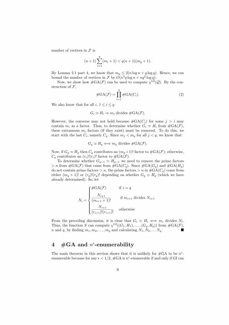
Figure 1: Combining ri copies of Gi and Hi.

the q prime numbers immediately following the number n. Let ri = (mi +1)/2.Assuming that each graph in Q has at least 2 vertices, ri is an integer. For eachi, 1 ≤ i ≤ q, we construct a graph Ci as follows. Take ri copies of Gi, ri copiesof Hi and a complete graph with 2ri new vertices a1, . . . , a2ri

. Connect eachvertex in the jth copy of Gi to aj . Connect each vertex in the jth copy of Hi

to ari+j . (See Figure 1.) Call the resulting graph Ci.Now, suppose that Gi is isomorphic to Hi. Then every automorphism of Ci

can be formed by a permutation of the vertices in a1, . . . , a2ri followed by an

automorphism of each copy of Gi and Hi. Hence

#GA(Ci) = (2ri)!(#GA(Gi))2ri .

Since 2ri = mi + 1, the prime number mi divides #GA(Ci).On the other hand, if Gi is not isomorphic to Hi then every automorphism

of Ci can be formed by a permutation of the vertices in a1, . . . , ari, followed

by a permutation of the vertices in ari+1, . . . , a2ri and the automorphisms of

each copy of Gi and Hi. In this case,

#GA(Ci) = (ri)!(ri)!(#GA(Gi))ri(#GA(Hi))ri .

Since ri < mi and |Gi| = |Hi| = n < mi, the prime number mi does not divide#GA(Ci). In summary,

Gi ' Hi ⇐⇒ mi divides #GA(Ci). (1)

Let F be the disjoint union of all the Ci, for 1 ≤ i ≤ q. The output of thefunction T (Q) will be F . Since each Ci has (mi + 1)(n + 1) vertices, the total

8

number of vertices in F is

(n+ 1)q∑

i=1

(mi + 1) < q(n+ 1)(mq + 1).

By Lemma 2.1 part 4, we know that mq ≤ 2(n log n + q log q). Hence, we canbound the number of vertices in F by O(n2q log n+ nq2 log q).

Now, we show how #GA(F) can be used to compute χGI(Q). By the con-struction of F ,

#GA(F) =q∏

i=1

#GA(Ci). (2)

We also know that for all i, 1 ≤ i ≤ q

Gi ' Hi ⇒ mi divides #GA(F).

However, the converse may not hold because #GA(Cj) for some j > i maycontain mi as a factor. Thus, to determine whether Gi ' Hi from #GA(F),these extraneous mi factors (if they exist) must be removed. To do this, westart with the last Ci, namely Cq. Since mj < mq for all j < q, we know that

Gq ' Hq ⇐⇒ mq divides #GA(F).

Now, if Gq ' Hq then Cq contributes an (mq +1)! factor to #GA(F); otherwise,Cq contributes an (ri)!(ri)! factor to #GA(F).

To determine whether Gq−1 ' Hq−1 we need to remove the prime factors> n from #GA(F) that came from #GA(Cq). Since #GA(Gq) and #GA(Hq)do not contain prime factors > n, the prime factors > n in #GA(Cq) come fromeither (mq + 1)! or (rq)!(rq)! depending on whether Gq ' Hq (which we havealready determined). So, let

Ni =

#GA(F) if i = q

Ni+1

(mi+1 + 1)!if mi+1 divides Ni+1

Ni+1

(ri+1)!(ri+1)!otherwise

From the preceding discussion, it is clear that Gi ' Hi ⇐⇒ mi divides Ni.Thus, the function S can compute χGI((G1,H1), . . . , (Gq,Hq)) from #GA(F),n and q, by finding m1,m2, . . . ,mq and calculating N1, N2, . . . Nq.

4 #GA and nε-enumerability

The main theorem in this section shows that it is unlikely for #GA to be nε-enumerable because for any ε < 1/2, #GA is nε-enumerable if and only if GI can

9

be recognized in polynomial time. We begin with a review of two constructionsfrom the literature. The first one shows that the Graph Isomorphism problemis “self-computable,” in the sense that given GI as an oracle, we can constructan isomorphism between two isomorphic graphs in polynomial time [KST93,Sch76]. We reproduce the proof of this well-known theorem because we needto make references to the construction in the proof and because we need toestimate the sizes of the graphs queried.

Lemma 4.1 There exists a polynomial-time Turing machine using GI as anoracle which finds an isomorphism between two graphs, if the graphs are iso-morphic.

Proof: We prove that GI is “self-computable” by constructing a mapping be-tween the vertices of two isomorphic graphs G and H using GI as an oracle.This “self-computable” property is similar to the disjunctive self-reducibility ofSAT.7 In the first stage of the construction, we find a vertex i1 in H such thatthere is an isomorphism between G and H mapping vertex 1 in G to vertex i1 inH. This is accomplished by trying all n vertices in H exhaustively and askingthe GI oracle the n questions:

Is there an isomorphism from G to H mapping vertex 1 to vertexi1?

These questions can be transformed into queries to GI by attaching cycles withn + 1 vertices to vertex 1 in G and vertex i1 in H. Thus, any isomorphismbetween the transformed graphs must map vertex 1 in G to vertex i1 in H. Ifsuch an isomorphism exists, the remaining n−1 stages of the construction assignvertices 2, . . . , n in G to the vertices in H under the restriction that vertex 1maps to vertex i1. In stage k of the construction, vertex k in G and ik in Hwill be attached to a cycle with n+ k vertices.

Remark: It is convenient to think of the procedure described in the precedingproof as a self-reduction tree. The root of the tree, level 0, is labeled with thegraphs (G,H). Each vertex at level k has n − k children which represent then − k possible assignments of vertex k in G to the n − k remaining verticesin H. These vertices are labeled with the corresponding transformed graphs.This tree has n! leaves, so we cannot construct the entire tree in polynomialtime. However, at the leaves of the tree, every vertex of G is assigned to somevertex of H. Thus, in polynomial time we can determine whether the mappingrepresented by a leaf is indeed an isomorphism between G and H.

In the proof of Theorem 4.5 below, our strategy is to traverse the self-reduction tree from the top down. Since the tree has exponentially many paths,

7That is, given any Boolean formula F , consider the formula F0 obtained by replacing thefirst variable of F with the Boolean value FALSE and the formula F1 obtained by replacingthe first variable with TRUE. Then, F ∈ SAT if and only if F0 ∈ SAT or F1 ∈ SAT (q.v.[BDG88, Section 4.5] and [Sch85, Section 4.5]).

10

we will need to identify some of the paths as dead-ends. The following com-binatorial lemmas [Bei91, Owi89] will help us prune the tree and maintain apolynomial bound on the running time of the tree traversal.

Definition 4.2 For a collection C of sets and a set X, we say X separates C iffor all S, S′ ∈ C, S 6= S′ ⇒ S ∩X 6= S′ ∩X.

Lemma 4.3 For a collection C of sets, with |C| = n ≥ 1, there exists a set Xthat separates C where |X| ≤ n− 1.

The lemma below adapts Lemma 4.3 to show that if we have ` vectorsin 0, 1`, then the vectors can be uniquely identified by their values at ` − 1coordinates. Thus, one of the coordinates is not needed to distinguish the vectorsfrom each other. In the following, we use (~b)i to denote the ith component of avector ~b ∈ Σ`.

Lemma 4.4 Let m ≤ ` and ~b1, . . . ,~bm ∈ 0, 1`. There exists a coordinate ksuch that for all ~bi 6= ~bj, there exists t 6= k such that (~bi)t 6= (~bj)t. Moreover, kcan be found in time polynomial in `.

Proof: It suffices to prove the case where m = `. Use Lemma 4.3 where C isthe collection of subsets of 1, . . . , ` represented by the bit vectors ~b1, . . . ,~b`.Let k be an element not contained in the separator X. Since X is a separator,each pair of bit vectors must differ at coordinates other than k. The coordinatek can be found in time polynomial in ` because we can simply try all possiblevalues for k and check each pair of ~bi and ~bj . This takes time O(`4).

We are now ready to prove the main result of this section. The techniquesused in this proof and in Lemma 4.4 are derived from results on enumerabilityand self-reducibility by Amir, Beigel and Gasarch [ABG90].

Theorem 4.5 For ε < 1/2, the function #GA is nε-enumerable if and only ifGI ∈ P.8

Proof: In Section 2, we outlined a polynomial-time algorithm for #GA whichuses GI as an oracle. Thus, if GI ∈ P, then #GA is also computable in polyno-mial time. In this case, #GA would be 1-enumerable. Thus, we only need toshow that if #GA is nε-enumerable, then GI ∈ P.

Given two graphs G and H with n vertices, we search the self-reduction treedescribed above in stages. We maintain a list Q of pairs of graphs from theself-reduction tree. Initially, Q contains just the pair (G,H). Throughout thetree-pruning procedure we maintain the invariant that G ' H if and only ifQ contains a pair of isomorphic graphs (i.e., χGI(Q) is not all zeroes). Also,the size of the list Q will always be polynomially bounded. In the beginning of

8Recall that the n in “nε-enumerable” is the number of vertices in the graph. If n is thelength of the encoding of the graph, we would need to further restrict ε < 1/4.

11

every stage of the tree pruning, we take each pair of graphs in Q and replace itwith its children in the self-reduction tree. We continue the replacement untilQ has at least q(n) pairs (for q(n) ≥ n to be determined below).

Let Q′ = 〈(G1,H1), . . . , (Gq(n),Hq(n))〉 be the first q(n) pairs in Q. Let m bean upper bound on the size of these graphs. We apply the Combining Lemma toconstruct the graph F which has at most r = mq(n)2 log q(n) vertices. Then, weuse the enumerator for #GA on F to obtain a list of rε numbers one of which is#GA(F). The function S in the Combining Lemma converts these numbers intoa list of rε vectors~b1, . . . ,~brε in 0, 1q(n), one of which is χGI(Q′). Now, supposethat ~bi 6= 0q(n) for all i, 1 ≤ i ≤ rε. Then, we know that χGI(Q′) 6= 0q(n), soG must be isomorphic to H. Thus, we can halt the pruning procedure andaccept. In the remaining case, we may assume that 0q(n) is one of the vectorsin ~b1, . . . ,~brε . We will pick q(n) below so that rε ≤ q(n). Then, Lemma 4.4gives us a coordinate k such that for ~bi 6= ~bj , the vectors ~bi and ~bj differ on acoordinate other than k. Now, it cannot be the case that (Gk,Hk) is the onlyisomorphic pair of graphs in Q′, because in that case χGI(Q′) = 0k−110q(n)−k,hence χGI(Q′) can only be distinguished from 0q(n) using the kth coordinate.Thus, the pruning process can safely remove the pair (Gk,Hk) from the list Qand still guarantee that if Q contains an isomorphic pair before pruning, thenit also does after pruning.

We continue removing items from Q until it has fewer than q(n) pairs ofgraphs. Then we proceed to the next stage. After at most n stages, the pairs inQ are leaves of the self-reduction tree, so we can compute χGI(Q) in polynomialtime. By the invariant we have maintained, G ' H if and only if χGI(Q) is notall zeroes. Thus, we have shown that GI ∈ P.

Finally, we need to show that by picking q(n) to be nα where α > 1/(1−2ε),we can guarantee that rε ≤ q(n). (The constant α is positive since ε < 1/2.)From the construction of the self-reduction tree in Lemma 4.1, we know that mis O(n2) since the graphs Gi and Hi consist of n original vertices and cycles ofsize n+ 1 through 2n. So,

rε ≤ (cn2 · q(n)2 · log q(n))ε = (cn2 · n2α · α log n)ε.

Thus, rε < n2ε+2αε+δ for all δ > 0. From our choice of α, we know that

2ε+ 2αε < 1 + 2αε < α.

Therefore, rε ≤ q(n).

Since it is generally believed that GI 6∈ P, the preceding theorem can also beinterpreted as a lower bound on the enumerability of #GA. We can also use thetheorem to obtain a lower bound on the bounded query complexity of #GA.The bounded query classes are defined as follows.

Definition 4.6 Let j(n) be a function and X be a set. A function f is inPFX[j(n)] if there exists a polynomial-time oracle Turing machine which com-putes f using no more than j(n) queries to X on inputs of length n.

12

Counting the number of oracle queries has been established as a useful com-plexity measure. For example, the number of queries to an NP oracle can beused to characterize the complexity of approximating NP-optimization problems[Cha96, CGL97]. The following fact shows that there is an intimate connectionbetween the enumerability of a function and the bounded query complexity ofthat function.

Fact 4.7 (Beigel [Bei87b, Lemma 3.2]) Let f be any function and j(n) be apolynomial-time computable function. The following are equivalent:

1. There exists X such that f ∈ PFX[j(n)].

2. f is 2j(n)-enumerable.

Using Fact 4.7 we can obtain a lower bound on the number of queries neededto compute #GA, assuming that GI 6∈ P.

Corollary 4.8 Let ε < 1/2. If there exists an X such that #GA ∈ PFX[ε log n]

then GI ∈ P.

5 #GA and poly-enumerability

Assuming that GI 6∈ P, the main result in the previous section is a “non-enumerability” result. In general, we would like to prove stronger non-enumerabilityresults for #GA. For example, Amir, Beigel and Gasarch [ABG90] were able toprove that #SAT is not 2nε

-enumerable for ε < 1 unless the Polynomial Hier-archy collapses. We cannot use their machinery for the case of #GA, becauseit turns out that #GA is actually exp(O(

√n log n))-enumerable. Instead, we

adapt the techniques of Goldwasser, Micali and Rackoff [GMR89] to show that#GA cannot be poly-enumerable unless GI ∈ R.9

Goldwasser, Micali and Rackoff showed that Graph Non-Isomorphism, thecomplement of GI, can be recognized by a two-round interactive protocol. Webriefly review this protocol in order to motivate the proof of Theorem 5.2. Thereare two parties involved in the interactive protocol: an all-powerful prover anda randomized polynomial-time verifier. The verifier asks the prover to convincehim that the input graphs (G,H) are not isomorphic as follows. In secret, theverifier randomly picks one of G and H along with a random permutation ψ. Heapplies ψ to either G or H, whichever one he picked, and obtains a new graphX. Then, the verifier asks the prover whether X is a permuted version of G orof H. If G and H are not isomorphic, the all-powerful prover simply checks ifG ' X or if H ' X, and provides the appropriate answer. On the other hand,if G and H are isomorphic, X can be a permuted version of either graph. Inthat case, the prover can only provide the correct answer with probability onehalf. Thus, if G 6' H, there exists a prover who can always convince the verifier

9We were motivated in part by Lozano and Toran [LT93, Theorem 5.1] who also used thistechnique in their proof.

13

to accept. Conversely, if G ' H, no prover (even one that “lies”) can convincethe verifier to accept with greater than 50 percent probability.

In the proof below, our randomized algorithm for GI will play the role of theverifier and the enumerator for #GA will play the role of the prover. However,unlike the prover in an interactive protocol, the enumerator provides severalanswers at once.10 Thus, it is possible for the enumerator to give two answersat the same time: one that corresponds to G ' H and one to G 6' H. We copewith this situation by emulating the interactive protocol many times in parallel.Thus, instead of picking one permutation ψ and forming one permuted graphX, we pick q(n) permutations ψ1, . . . ψq(n) and form q(n) graphs X1, . . . , Xq(n)

each of which is a permutation of either G or H.

Notation 5.1 For each permutation ψ ∈ Sn, we use ψ(G) to denote the graphobtained by re-labelling the vertices of G using ψ. Given two permutationsψ, ρ ∈ Sn, we define ψρ ∈ Sn to be the functional composition of ψ and ρ —i.e., (ψρ)(G) = ψ(ρ(G)).

Theorem 5.2 If #GA is poly-enumerable then GI ∈ R.

Proof: Assuming that #GA is p(n)-enumerable via an enumeration functiong, we will construct a randomized polynomial-time algorithm to decide whetherthe input graphs G and H are isomorphic. Let n be the number of vertices inG and H and let q(n) ≥ n be a polynomial to be specified later. As discussedabove, we randomly pick q(n) permutations ψ1, . . . , ψq(n) from Sn and for eachψi permute either G or H. Our choice of applying ψi to either G or H can berepresented by a single bit. So, a bit vector ~b ∈ 0, 1q(n) and the permutationsψ1, . . . , ψq(n) fully specify our random choices. Let bi be the ith bit of ~b and Xi

be the result of applying the permutation ψi; that is,

Xi =

ψi(H) if bi = 0ψi(G) if bi = 1.

Now, consider the instances of the graph isomorphism problem: (G,X1), . . . , (G,Xq(n)).Note that if G is not isomorphic to H then

χGI((G,X1), . . . , (G,Xq(n))) = ~b,

since G is isomorphic to Xi only when Xi = ψi(G). On the other hand, if Gis isomorphic to H, then our choice of applying ψi to G or H does not changewhether G is isomorphic to Xi. So, in this case,

χGI((G,X1), . . . , (G,Xq(n))) = 1q(n).

Next, we use the Combining Lemma on (G,X1), . . . , (G,Xq(n)) to construct agraph F such that #GA(F) provides enough information to compute χGI((G,X1), . . . , (G,Xq(n))).

10Another difference is that the enumerator cannot “lie” in the same manner as the proverbecause one of the answers it provides must be the correct value of #GA.

14

Procedure R-ISO(G,H)

1. Randomly pick ~b ∈ 0, 1q(n) and ψ1, . . . , ψq(n) ∈ Sn.

2. Use the Combining Lemma to construct F = T ((G,X1), . . . , (G,Xq(n))).

3. Use g to generate the possible values of #GA(F).

4. Compute the set POSS = S(n, q(n), N) | N ∈ g(F).

5. If ~b 6∈ POSS then output YES, otherwise output NO.

Figure 2: Randomized procedure to determine whether the graphs G and H areisomorphic.

Let r(n) be a polynomial upper bound on the number of vertices in F . If wecould compute #GA(F) directly, then we can immediately determine whetherG ' H by checking whether #GA(F) corresponds to the case where χGI((G,X1), . . . , (G,Xq(n)))is ~b or 1q(n).11 However, we cannot compute #GA(F) directly, so we use theenumerator for #GA(F) instead. Let T and S be the reduction functions fromthe Combining Lemma. (We used T on (G,X1), . . . , (G,Xq(n)) to obtain thegraph F .) Since we assume that #GA is p(n)-enumerable, in polynomial time wecan compute g(F), a set of polynomially many values one of which is #GA(F).For each value in g(F), we use the S function from the Combining Lemma todetermine a possible value for χGI((G,X1), . . . , (G,Xq(n))). Call the set of allsuch values

POSS = S(n, q(n), N) | N ∈ g(F) .

If G 6' H, then ~b = χGI((G,X1), . . . , (G,Xq(n))). Thus, ~b must be an element ofPOSS, since χGI((G,X1), . . . , (G,Xq(n))) is always an element of POSS. On theother hand, if G ' H, then ~b ∈ POSS occurs with very low probability. (Thiswill be proven below.) Therefore, the strategy for our randomized algorithm is toaccept (G,H) if and only if ~b 6∈ POSS. Figure 2 summarizes Procedure R-ISO,the randomized algorithm to determine whether G ' H.

If G 6' H, then Procedure R-ISO outputs NO with probability 1. We need toshow that if G ' H then Procedure R-ISO outputs YES with high probability.Intuitively, it is unlikely for ~b ∈ POSS when G ' H because POSS is completelydetermined by F and the same F can be the result of exponentially manyrandom choices. We prove this formally by showing that for each of choice of ~band ψ1, . . . , ψq(n) made by Procedure R-ISO, there is a block of 2q(n) randomchoices which produces the same graph F . Each random choice within a blockhas a distinct ~b. Thus, within each block, the probability that ~b ∈ POSS is atmost p(r(n))/2q(n). Furthermore, we will show that the blocks form a partition

11The exception is the pathological case where we chose ~b = 1q(n). However, this case onlyoccurs with probability 1/2q(n).

15

of the set of all random choices made by Procedure R-ISO. Thus, the overallprobability that ~b ∈ POSS is also bounded by p(r(n))/2q(n).

The blocks are defined as follows. Assume that G is isomorphic to H. Sincepermutations are invertible, for every graph Y isomorphic to G, there existsa permutation ρ such that ρ(H) = Y . Now, fix a sequence of permutationsσ1, . . . , σq(n) ∈ Sn and let Yi = σi(G). Let ρ1, . . . , ρq(n) be the correspondingpermutations such that ρi(H) = Yi. Let ~b be any bit vector chosen by Proce-dure R-ISO. Then, there exists a choice of ψ1, . . . , ψq(n) such that the graph Xi

constructed in Procedure R-ISO is exactly Yi, namely:

ψi =

ρi if bi = 0;σi if bi = 1.

Furthermore, if we fix an isomorphism τ from H to G, the permutation ψi iscompletely determined by bi and σi — i.e., ψi = σiτ if bi = 0 and ψi = σi

if bi = 1. Thus, we can associate the permutations σ1, . . . , σq(n) with a blockof 2q(n) random choices for Procedure R-ISO (since there are 2q(n) different bitvectors ~b). To see that every choice of ~b and ψ1, . . . , ψq(n) corresponds to someblock, simply note that we can set σi = ψiτ

−1 if bi = 0 and σi = ψi if bi = 1.This will again guarantee that Yi = Xi for every i. Therefore, the blocks doform a partition of the set of all random choices made by Procedure R-ISO.

Finally, observe that for each of the 2q(n) distinct bit vectors ~b in a block,the same instances of GI, (G,X1), . . . , (G,Xq(n)), are constructed by Proce-dure R-ISO. Thus, the same set POSS is generated. Since POSS has p(r(n))elements and since p(r(n)) is polynomially bounded, the probability that a ran-domly chosen ~b is not an element of POSS is at least 1 − p(r(n))/2q(n). Thus,for q(n) large enough, Procedure R-ISO will accept with high probability in thecase that G ' H.

As before, we can translate the non-enumerability of #GA into lower boundson its bounded query complexity using Fact 4.7.

Corollary 5.3 If there exists an X such that #GA ∈ PFX[O(log n)] then GI ∈R.

6 Subexponential enumeration

The results of the preceding section can be interpreted as lower bounds on theenumerability of #GA since it seems unlikely that GI ∈ P or GI ∈ R. In thissection we provide an upper bound on the enumerability of #GA by showingthat #GA is exp(O(

√n log n))-enumerable. Our enumerator will be oblivious.

That is, given a graph G with n vertices and an index `, the output of thisenumerator g(G, `) will depend only on n and `. We think of ` as being anencoding of the order of a permutation group A of degree n. We must showthat an appropriate encoding exists such that ` takes space O(

√n log n) and the

function ` 7→ |A| is computable in polynomial time.

16

Definition 6.1 Let Sn be the group of all permutations of Ω = 1, . . . , n undercomposition. A subgroup A of Sn, written A ≤ Sn, is also called a permutationgroup of degree n and Ω is called the permutation domain of A. The order ofthe subgroup A, written |A|, is the number of permutations in A.

Lemma 6.2 Let A be a subgroup of Sn. Let pi be the ith prime. Then |A| mustbe of the form

∏mi=1 p

dii where

1. for all i, di ≤ n.

2. m ≤ n/ lnn+ o(n/ lnn).

Proof: Let m and d1, . . . , dm be such that |A| =∏m

i=1 pdii . Since |A| is a divisor

of n!, we know that for all i, pdii divides n!. However, for any prime p, the highest

power of p dividing n! is pd, where

d =∑j≥1

⌊n

pj

⌋< n

∑j≥1

1pj

=n

p− 1≤ n.

(This formula simply counts the number of positive integers up to n which aredivisible by p, p2, et cetera.) In particular, all the prime factors of |A| are ≤ n.The Prime Number Theorem states that

limn→∞

π(n)n/ lnn

= 1,

where π(n) is the number of primes less than or equal to n. Thus, m ≤ n/ lnn+o(n/ lnn).

Theorem 6.3 #GA is exp(O(√n log n))-enumerable via an oblivious enumer-

ator.

Proof: Let G be a graph. The set of automorphisms of G is a subgroup of Sn,hence #GA(G) must be of the form specified in Lemma 6.2. We show how toenumerate all possible sizes of the subgroups of Sn. We describe this in the formof a compressed encoding of orders of subgroups of Sn, such that the encodinglengths are O(

√n log n) and given the encoding of |A|, we can compute |A|

in polynomial time. One method would be to simply write down the binaryrepresentations of the di, for 1 ≤ i ≤ π(n). By Lemma 6.2 the number of bitsused would be O(n), which is too many. However, we will use this technique for“small” primes.

Let k =√n log n. Then π(k) = O(k/ log n) = O(

√n/ log n). For A ≤ Sn,

the first part of the encoding of A will consist of the binary representationsof the di for pi ≤ k. This uses O(π(k) log n) = O(

√n log n) bits, as desired.

To encode the exponents of the larger primes, we must use detailed knowledgeof the possible orders of subgroups of Sn. However, our task will be greatlysimplified by the fact that we can now ignore the small primes.

17

Let Ω denote 1, . . . , n. For x ∈ Ω, xA denotes the A-orbit of x defined by:

xA = y ∈ Ω | (∃ψ ∈ A)[y = ψ(x)] .

We say that an orbit is trivial if it has one element, and we say that A istransitive if Ω is an orbit. In any case, the A-orbits partition Ω. We describetwo divide-and-conquer techniques based on this partition. Let ∆ = xA bean A-orbit, and let Ax denote the subgroup ψ ∈ A | ψ(x) = x of thosepermutations which fix x. It is well known that

|A| = |Ax| · |∆|,

so if |∆| has only prime factors ≤ k, we may replace A by Ax for the purposes ofthe second part of the encoding. We henceforth assume that all nontrivial orbitsof A have orders divisible by some prime larger than k (so in particular thereare at most

√n/ log n nontrivial orbits). Actually, we make the more general

assumption that for any proper subgroup B of A, the index |A|/|B| is divisibleby a prime larger than k.

Now suppose that |∆| = m, and let B be the subgroup of Sm obtained fromA by ignoring the action outside of ∆. That is, B consists of those permutationsψ ∈ Sm for which there exist ψ′ ∈ A such that ψ′ is an extension of ψ. Let A∆

denote the subgroup of A which fixes every point of ∆ (i.e., A is the subgroupof pointwise stabilizers of ∆ in A). Then |A| = |B| · |A∆|, and to encode |A|it suffices to first encode |B| and then recursively encode |A∆|. The number oforbits ∆ which need to be considered is O(

√n/ log n), so we must use no more

than O(log n) bits to encode |B|. To do this, we make great use of the fact thatB is transitive.

Now suppose that ∆1, . . . ,∆r is a partition of ∆ with 1 < r < m suchthat B permutes the ∆i. If several such partitions exist, then choose one thatminimizes r. Then the partition is called a system of imprimitivity for B, andthe ∆i are called blocks of imprimitivity. Since B acts transitively on the set ofblocks, B has a subgroup of index r, from which we conclude that r is divisibleby some prime p > k. Let N be the subgroup of B that fixes the blocks, i.e. anyx ∈ N sends each ∆i to itself. Let K be the subgroup of Sr obtained from B byconsidering the action on the blocks. Then |B| = |N | · |K|. In addition, everyorbit of N has order less than k, so |N | is a product of primes whose values areat most k. Thus, to encode |B|, it suffices to encode |K|. By minimality of r, Kis primitive, i.e., preserves no nontrivial partition of the permutation domain.

Much is already known about the structure of primitive groups. The O’Nan–Scott Lemma [Cam81, Theorem 4.1] classifies them into several types. Many ofthese are ruled out by our assumption that the index of any proper subgroupof K is divisible by some prime larger than k (where k2 is bigger than r, thesize of the permutation domain). In fact, it must be the case that K has asimple normal subgroup T . Further, either |T | = r and K is a subgroup of theautomorphism group of T × T , or K is a subgroup of the automorphism groupof T . Following the Classification of Finite Simple groups, much is known aboutthe permutation representations of finite simple groups [BKL83]. In particular,

18

either T is one of polynomially many alternating or classical groups (each ofwhich can be described by a string of length O(log n)), or |K| is polynomiallybounded. In the first case |K|/|T | is polynomially bounded, so in either caseO(log n) bits suffice to describe the order of K.

We summarize the encoding of |A|. First, we write down the binary repre-sentations of the exponents of the primes in |A| for all primes p ≤ k. Then, wewrite down a sequence of O(n/k) pairs (〈T 〉, N), where 〈T 〉 is an O(log n) lengthname of a group T which is either the trivial group or a classical group with apermutation representation of degree ≤ n and N is a positive integer (written inbinary) which is at most nc for some constant c. For primes p > k, the p-part of|A| is the product of the p-parts of the N ’s and the orders of the T ’s. The orderof T is given by an explicit formula, so |A| can be computed in polynomial timefrom its encoding. The first part of the encoding uses O(π(k) log n) bits; thesecond part of the encoding uses O((n/k) log n) bits. Both of these quantitiesare O(

√n log n) as desired.

7 Discussion

Several open problems remain on the enumerability of #GA. We have shownthat if #GA is poly-enumerable, then GI ∈ R. For SAT, we know that if #SATpoly-enumerable, then P = PP [ABG90, CH91] which implies that SAT ∈ P.For #GA, it remains open whether #GA being poly-enumerable could implythat GI ∈ P. It might even be possible to show that if #GA is 2nε

-enumerablefor some ε < 1/2, then GI ∈ P. Such a theorem would not violate our up-per bound that #GA is exp(O(

√n log n))-enumerable. Note that an analogous

result for #SAT, that #SAT is 2nε

-enumerable implies SAT ∈ P, is not known.While no polynomial-time algorithms for GI or #GA have been discovered,

algorithms with subexponential running time do exist. For example, there ex-ists an algorithm with time complexity exp(O(

√n log n)) which computes the

automorphism group and its generators [BKL83] (this is harder than solvingGI and #GA). This algorithm combines the techniques of several authors in-cluding Babai, Luks, and Zemlyachenko. The bound on the running time isthe same as the upper bound on the enumerability of #GA that we achievedin Section 6. This striking observation brings up the possibility of the follow-ing time-enumeration trade-off. By allowing the enumerator to run for longerthan polynomial time, say time exp(O((n log n)a + log n)), it might be possi-ble to achieve exp(O((n log n)b))-enumerability for a + b = 1/2. Note that thecase a = 1/2 is given by the subexponential-time algorithm mentioned above[BKL83], and the case a = 0 is our upper bound. The case 0 < a < 1/2 is open.

We remark that for oblivious enumeration, our upper bound is tight up tosome logarithmic factors in the exponent. To see this, let k =

√n log n as in

Section 6. Since kπ(k) = O(n), the sum of the primes up to k is O(n). Byscaling k by a constant factor, we may achieve that π(k) = Ω(

√n/ log n) and

the sum of the primes less than k is ≤ n. So, for any subset S of the primes

19

p ≤ k, there is a permutation group of degree n whose order is the product of theprimes in S (the group is generated by disjoint cycles of prime lengths). Thisgives us exp(Ω(

√n/ log n)) different orders of permutation groups of degree

n. It is straightforward to obtain the same lower bound for the number ofdistinct orders of automorphism groups of graphs of degree n. Thus, obliviousenumeration seems to have reached its limit, but it remains open whether ornot a clever use of polynomial-time computable graph properties would yield abetter, non-oblivious enumerator.

Finally, we note that the reduction of Section 5 can be used even if theenumeration is not polynomial. (It would yield a randomized algorithm for GIwhich has super-polynomial running time.) Roughly speaking, the reductioncan be used as long as the enumerability is less than about exp(n1/2−ε) (so,not surprisingly, an oblivious enumerator is useless for this). In order to beatthe subexponential running time of the existing algorithm [BKL83], the enu-merability would have to be about exp(n1/4−ε) (however, the enumerator wouldnot have to be restricted to polynomial time).

Acknowledgements

The authors would like to thank Laszlo Babai for helpful comments on the topicsof this paper, and Dave Mount for proofreading.

References

[ABG90] A. Amir, R. Beigel, and W. I. Gasarch. Some connections betweenbounded query classes and non-uniform complexity. In Proceedingsof the 5th Structure in Complexity Theory Conference, pages 232–243,1990. A much expanded version has been submitted to Information andComputation and is available via http://www.eecs.lehigh.edu/ beigel/.

[BDG88] J. L. Balcazar, J. Dıaz, and J. Gabarro. Structural Complexity I,volume 11 of EATCS Monographs on Theoretical Computer Science.Springer-Verlag, 1988.

[BDG90] J. L. Balcazar, J. Dıaz, and J. Gabarro. Structural Complexity II,volume 22 of EATCS Monographs on Theoretical Computer Science.Springer-Verlag, 1990.

[Bei87a] R. Beigel. Query-Limited Reducibilities. PhD thesis, Stanford Univer-sity, 1987. Also available as Report No. STAN-CS-88-1221.

[Bei87b] R. Beigel. A structural theorem that depends quantitatively on thecomplexity of SAT. In Proceedings of the 2nd Structure in ComplexityTheory Conference, pages 28–32, June 1987.

[Bei91] R. Beigel. Bounded queries to SAT and the Boolean hierarchy. Theo-retical Computer Science, 84(2):199–223, July 1991.

20

[BGM82] L. Babai, Y. Grigoryev, and D. Mount. Isomorphism testing forgraphs with bounded eigenvalue multiplicities. In ACM Symposiumon Theory of Computing, pages 310–324, 1982.

[BKL83] L. Babai, W. M. Kantor, and E. M. Luks. Computational complexityand the classification of finite simple groups. In Proceedings of the IEEESymposium Foundations of Computer Science, pages 162–171, 1983.

[Cam81] P. J. Cameron. Finite permutation groups and finite simple groups.Bulletin of the London Mathematical Society, 13:1–22, 1981.

[CGL97] R. Chang, W. I. Gasarch, and C. Lund. On bounded queries andapproximation. SIAM Journal on Computing, 26(1):188–209, February1997.

[CH89] J. Cai and L. A. Hemachandra. Enumerative counting is hard. Infor-mation and Computation, 82(1):34–44, July 1989.

[CH91] J. Cai and L. A. Hemachandra. A note on enumerative counting. In-formation Processing Letters, 38(4):212–219, 1991.

[Cha96] R. Chang. On the query complexity of clique size and maximum sat-isfiability. Journal of Computer and System Sciences, 53(2):298–313,October 1996.

[FM80] I. S. Filotti and J. N. Mayer. A polynomial-time algorithm for deter-mining the isomorphism of graphs of fixed genus. In ACM Symposiumon Theory of Computing, pages 236–243, 1980.

[GMR89] S. Goldwasser, S. Micali, and C. Rackoff. The knowledge complexityof interactive proof systems. SIAM Journal on Computing, 18(1):186–208, 1989.

[Hof79] C. M. Hoffman. Group-Theoretic Algorithms and Graph Isomorphism,volume 136 of Lecture Notes in Computer Science. Springer-Verlag,1979.

[HT71] J. E. Hopcroft and R. E. Tarjan. A V 2 algorithm for determiningisomorphism of planar graphs. Information Processing Letters, pages32–34, 1971.

[HW74] J. E. Hopcroft and J. K. Wong. A linear time algorithm for isomorphismof planar graphs. In ACM Symposium on Theory of Computing, pages172–184, 1974.

[HW79] G. Hardy and E. Wright. An Introduction to the Theory of Numbers.Clarendon Press, Oxford, fifth edition, 1979. The first edition waspublished in 1938.

[Kre88] M. W. Krentel. The complexity of optimization problems. Journal ofComputer and System Sciences, 36(3):490–509, 1988.

21

[KST93] J. Kobler, U. Schoning, and J. Toran. The Graph Isomorphism Prob-lem: Its Structural Complexity. Progress in Theoretical Computer Sci-ence. Birkhauser, Boston, 1993.

[LT93] A. Lozano and J. Toran. On the nonuniform complexity of the graphisomorphism problem. In K. Ambos-Spies, S. Homer, and U. Schoning,editors, Complexity Theory: Current Research, pages 245–273. Cam-bridge University Press, 1993. Shorter version in Proceedings of the 7thStructure in Complexity Theory Conference, pages 118–129, June 1992.

[Luk82] E. Luks. Isomorphism of bounded valence can be tested in polynomialtime. Journal of Computer and System Sciences, 25:42–65, 1982.

[Mat79] R. Mathon. A note on the graph isomorphism counting problem. In-formation Processing Letters, 8:131–132, 1979.

[Mil80] G. L. Miller. Isomorphism testing for graphs of bounded genus. InACM Symposium on Theory of Computing, pages 225–235, 1980.

[Owi89] J. C. Owings, Jr. A cardinality version of Beigel’s nonspeedup theorem.Journal of Symbolic Logic, 54(3):761–767, September 1989.

[RS62] J. B. Rosser and L. Schoenfeld. Approximate formulas for some func-tions of prime numbers. Illinois Journal of Mathematics, 6:64–94, 1962.

[Sch76] C. P. Schnorr. Optimal algorithms for self-reducible problems. In Pro-ceedings of the 3rd International Conference on Automata, Language,and Programming (ICALP), pages 322–337, 1976.

[Sch85] U. Schoning. Complexity and Structure, volume 211 of Lecture Notesin Computer Science. Springer-Verlag, 1985.

[Sch89] U. Schoning. Probabilistic complexity classes and lowness. Journal ofComputer and System Sciences, 39(1):84–100, December 1989.

[Tod91] S. Toda. PP is as hard as the polynomial-time hierarchy. SIAM Journalon Computing, 20(5):865–877, October 1991.

[Val79] L. G. Valiant. The complexity of computing the permanent. TheoreticalComputer Science, 8:189–201, 1979.

22