Finding Patterns inThree-Dimensional Graphs: Algorithms and

Applications to Scientific Data MiningXiong Wang, Member, IEEE, Jason T.L. Wang, Member, IEEE,

Dennis Shasha, Bruce A. Shapiro, Isidore Rigoutsos, Member, IEEE, and Kaizhong Zhang

AbstractÐThis paper presents a method for finding patterns in 3D graphs. Each node in a graph is an undecomposable or atomic unit

and has a label. Edges are links between the atomic units. Patterns are rigid substructures that may occur in a graph after allowing for

an arbitrary number of whole-structure rotations and translations as well as a small number (specified by the user) of edit operations in

the patterns or in the graph. (When a pattern appears in a graph only after the graph has been modified, we call that appearance

ªapproximate occurrence.º) The edit operations include relabeling a node, deleting a node and inserting a node. The proposed method

is based on the geometric hashing technique, which hashes node-triplets of the graphs into a 3D table and compresses the label-

triplets in the table. To demonstrate the utility of our algorithms, we discuss two applications of them in scientific data mining. First, we

apply the method to locating frequently occurring motifs in two families of proteins pertaining to RNA-directed DNA Polymerase and

Thymidylate Synthase and use the motifs to classify the proteins. Then, we apply the method to clustering chemical compounds

pertaining to aromatic, bicyclicalkanes, and photosynthesis. Experimental results indicate the good performance of our algorithms and

high recall and precision rates for both classification and clustering.

Index TermsÐKDD, classification and clustering, data mining, geometric hashing, structural pattern discovery, biochemistry,

medicine.

æ

1 INTRODUCTION

STRUCTURAL pattern discovery finds many applications innatural sciences, computer-aided design, and image

processing [8], [33]. For instance, detecting repeatedlyoccurring structures in molecules can help biologists tounderstand functions of the molecules. In these domains,molecules are often represented by 3D graphs. The tertiarystructures of proteins, for example, are 3D graphs [5], [9],[18]. As another example, chemical compounds are also3D graphs [21].

In this paper, we study a pattern discovery problem for

graph data. Specifically, we propose a geometric hashing

technique to find frequently occurring substructures in a set

of 3D graphs. Our study is motivated by recent advances in

the data mining field, where automated discovery ofpatterns, classification and clustering rules is one of themain tasks. We establish a framework for structural patterndiscovery in the graphs and apply our approach toclassifying proteins and clustering compounds. While thedomains chosen here focus on biochemistry, our approachcan be generalized to other applications where graph dataoccur commonly.

1.1 3D Graphs

Each node of the graphs we are concerned with is anundecomposable or atomic unit and has a 3D coordinate.1

Each node has a label, which is not necessarily unique in agraph. Node labels are chosen from a domain-dependentalphabet �. In chemical compounds, for example, thealphabet includes the names of all atoms. A node can beidentified by a unique, user-assigned number in the graph.Edges in the graph are links between the atomic units. Inthe paper, we will consider 3D graphs that are connected.For disconnected graphs, we consider their connectedcomponents [16].

A graph can be divided into one or more rigid

substructures. A rigid substructure is a subgraph in whichthe relative positions of the nodes in the substructure arefixed, under some set of conditions of interest. Note that therigid substructure as a whole can be rotated (we refer to thisas a ªwhole-structureº rotation or simply a rotation whenthe context is clear). Thus, the relative position of a node in

IEEE TRANSACTIONS ON KNOWLEDGE AND DATA ENGINEERING, VOL. 14, NO. 4, JULY/AUGUST 2002 731

. X. Wang is with the Department of Computer Science, California StateUniversity, Fullerton, CA 92834. E-mail: wang@ecs.fullerton.edu.

. J.T.L. Wang is with the Department of Computer and Information Science,New Jersey Institute of Technology, University Heights, Newark, NJ07102. E-mail: jason@cis.njit.edu.

. D. Shasha is with the Courant Institute of Mathematical Sciences, NewYork University, 251 Mercer St., New York, NY 10012.E-mail: shasha@cs.nyu.edu.

. B.A. Shapiro is with the Laboratory of Experimental and ComputationalBiology, Division of Basic Sciences, National Cancer Institutes, Frederick,MD 21702. E-mail: bshapiro@ncifcrf.gov.

. I. Rigoutsos is with the IBM T.J. Watson Research Center, YorktownHeights, NY 10598. E-mail: rigoutso@us.ibm.com.

. K. Zhang is with the Department of Computer Science, The University ofWestern Ontario, London, Ontario, Canada N6A 5B7.E-mail: kzhang@csd.uwo.ca.

Manuscript received 19 May 1999; revised 18 Oct. 2000; accepted 18 Jan.2001; posted to Digital Library 7 Sept. 2001.For information on obtaining reprints of this article, please send e-mail to:tkde@computer.org, and reference IEEECS Log Number 109849.

1. More precisely, the 3D coordinate indicates the location of the center ofthe atomic unit.

1041-4347/02/$17.00 ß 2002 IEEE

the substructure and a node outside the substructure can bechanged under the rotation. The precise definition of aªsubstructureº is application dependent. For example, inchemical compounds, a ring is often a rigid substructure.

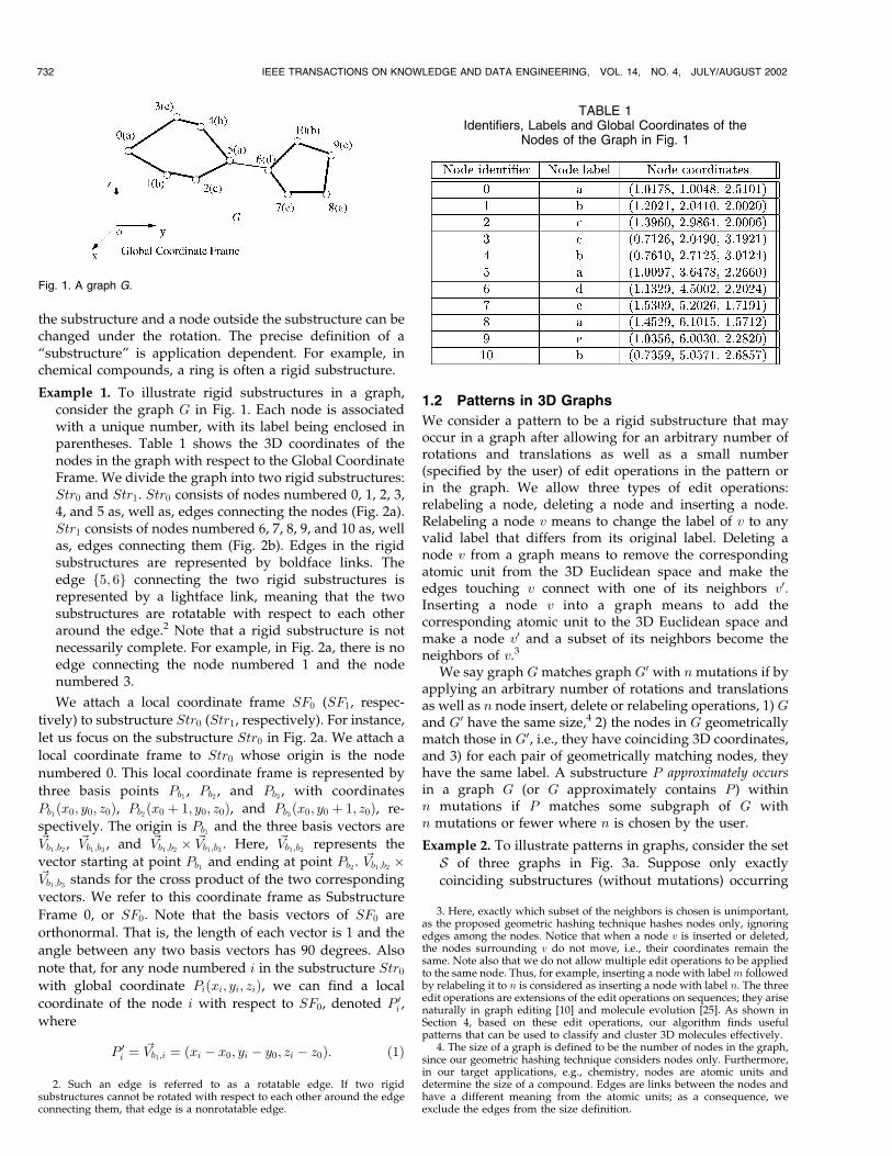
Example 1. To illustrate rigid substructures in a graph,consider the graph G in Fig. 1. Each node is associatedwith a unique number, with its label being enclosed inparentheses. Table 1 shows the 3D coordinates of thenodes in the graph with respect to the Global CoordinateFrame. We divide the graph into two rigid substructures:Str0 and Str1. Str0 consists of nodes numbered 0, 1, 2, 3,4, and 5 as, well as, edges connecting the nodes (Fig. 2a).Str1 consists of nodes numbered 6, 7, 8, 9, and 10 as, wellas, edges connecting them (Fig. 2b). Edges in the rigidsubstructures are represented by boldface links. Theedge f5; 6g connecting the two rigid substructures isrepresented by a lightface link, meaning that the twosubstructures are rotatable with respect to each otheraround the edge.2 Note that a rigid substructure is notnecessarily complete. For example, in Fig. 2a, there is noedge connecting the node numbered 1 and the nodenumbered 3.

We attach a local coordinate frame SF0 (SF1, respec-

tively) to substructure Str0 (Str1, respectively). For instance,

let us focus on the substructure Str0 in Fig. 2a. We attach a

local coordinate frame to Str0 whose origin is the node

numbered 0. This local coordinate frame is represented by

three basis points Pb1, Pb2

, and Pb3, with coordinates

Pb1�x0; y0; z0�, Pb2

�x0 � 1; y0; z0�, and Pb3�x0; y0 � 1; z0�, re-

spectively. The origin is Pb1and the three basis vectors are

~Vb1;b2, ~Vb1;b3

, and ~Vb1;b2� ~Vb1;b3

. Here, ~Vb1;b2represents the

vector starting at point Pb1and ending at point Pb2

. ~Vb1;b2�

~Vb1;b3stands for the cross product of the two corresponding

vectors. We refer to this coordinate frame as Substructure

Frame 0, or SF0. Note that the basis vectors of SF0 are

orthonormal. That is, the length of each vector is 1 and the

angle between any two basis vectors has 90 degrees. Also

note that, for any node numbered i in the substructure Str0

with global coordinate Pi�xi; yi; zi�, we can find a local

coordinate of the node i with respect to SF0, denoted P 0i ,where

P 0i � ~Vb1;i � �xi ÿ x0; yi ÿ y0; zi ÿ z0�: �1�

1.2 Patterns in 3D Graphs

We consider a pattern to be a rigid substructure that mayoccur in a graph after allowing for an arbitrary number ofrotations and translations as well as a small number(specified by the user) of edit operations in the pattern orin the graph. We allow three types of edit operations:relabeling a node, deleting a node and inserting a node.Relabeling a node v means to change the label of v to anyvalid label that differs from its original label. Deleting anode v from a graph means to remove the correspondingatomic unit from the 3D Euclidean space and make theedges touching v connect with one of its neighbors v0.Inserting a node v into a graph means to add thecorresponding atomic unit to the 3D Euclidean space andmake a node v0 and a subset of its neighbors become theneighbors of v.3

We say graph G matches graph G0 with n mutations if byapplying an arbitrary number of rotations and translationsas well as n node insert, delete or relabeling operations, 1) Gand G0 have the same size,4 2) the nodes in G geometricallymatch those in G0, i.e., they have coinciding 3D coordinates,and 3) for each pair of geometrically matching nodes, theyhave the same label. A substructure P approximately occursin a graph G (or G approximately contains P ) withinn mutations if P matches some subgraph of G withn mutations or fewer where n is chosen by the user.

Example 2. To illustrate patterns in graphs, consider the set

S of three graphs in Fig. 3a. Suppose only exactlycoinciding substructures (without mutations) occurring

732 IEEE TRANSACTIONS ON KNOWLEDGE AND DATA ENGINEERING, VOL. 14, NO. 4, JULY/AUGUST 2002

Fig. 1. A graph G.

TABLE 1Identifiers, Labels and Global Coordinates of the

Nodes of the Graph in Fig. 1

2. Such an edge is referred to as a rotatable edge. If two rigidsubstructures cannot be rotated with respect to each other around the edgeconnecting them, that edge is a nonrotatable edge.

3. Here, exactly which subset of the neighbors is chosen is unimportant,as the proposed geometric hashing technique hashes nodes only, ignoringedges among the nodes. Notice that when a node v is inserted or deleted,the nodes surrounding v do not move, i.e., their coordinates remain thesame. Note also that we do not allow multiple edit operations to be appliedto the same node. Thus, for example, inserting a node with label m followedby relabeling it to n is considered as inserting a node with label n. The threeedit operations are extensions of the edit operations on sequences; they arisenaturally in graph editing [10] and molecule evolution [25]. As shown inSection 4, based on these edit operations, our algorithm finds usefulpatterns that can be used to classify and cluster 3D molecules effectively.

4. The size of a graph is defined to be the number of nodes in the graph,since our geometric hashing technique considers nodes only. Furthermore,in our target applications, e.g., chemistry, nodes are atomic units anddetermine the size of a compound. Edges are links between the nodes andhave a different meaning from the atomic units; as a consequence, weexclude the edges from the size definition.

in at least two graphs and having size greater than three

are considered as ªpatterns.º Then, S contains one

pattern shown in Fig. 3b. If substructures having size

greater than four and approximately occurring in all the

three graphs within one mutation (i.e., one node delete,

insert, or relabeling is allowed in matching a substruc-

ture with a graph) are considered as ªpatterns,º then Scontains one pattern shown in Fig. 3c.

Our strategy to find the patterns in a set of 3D graphs is

to decompose the graphs into rigid substructures and, then,

use geometric hashing [14] to organize the substructures

and, then, to find the frequently occurring ones. In [35], we

applied the approach to the discovery of patterns in

chemical compounds under a restricted set of edit opera-

tions including node insert and node delete, and tested the

quality of the patterns by using them to classify thecompounds. Here, we extend the work in [35] by

1. considering more general edit operations includingnode insert, delete, and relabeling,

2. presenting the theoretical foundation and evaluatingthe performance and efficiency of our pattern-finding algorithm,

3. applying the discovered patterns to classifying3D proteins, which are much larger and morecomplicated in topology than chemical compounds,and

4. presenting a technique to cluster 3D graphs based onthe patterns occurring in them.

Specifically, we conducted two experiments. In the firstexperiment, we applied the proposed method to locatingfrequently occurring motifs (substructures) in two familiesof proteins pertaining to RNA-directed DNA Polymeraseand Thymidylate Synthase, and used the motifs to classifythe proteins. Experimental results showed that our methodachieved a 96.4 percent precision rate. In the secondexperiment, we applied our pattern-finding algorithm todiscovering frequently occurring patterns in chemicalcompounds chosen from the Merck Index pertaining toaromatic, bicyclicalkanes and photosynthesis. We then usedthe patterns to cluster the compounds. Experimental resultsshowed that our method achieved 99 percent recall andprecision rates.

The rest of the paper is organized as follows: Section 2presents the theoretical framework of our approach and

WANG ET AL.: FINDING PATTERNS IN THREE-DIMENSIONAL GRAPHS: ALGORITHMS AND APPLICATIONS TO SCIENTIFIC DATA MINING 733

Fig. 2. The rigid substructures of the graph in Fig. 1.

Fig. 3. (a) The set S of three graphs, (b) the pattern exactly occurring in two graphs in S, and (c) the pattern approximately occurring, within one

mutation, in all the three graphs.

describes the pattern-finding algorithm in detail. Section 3

evaluates the performance and efficiency of the pattern-finding algorithm. Section 4 describes the applications of

our approach to classifying proteins and clustering com-

pounds. Section 5 discusses related work. Section 6

concludes the paper.

2 PATTERN-FINDING ALGORITHM

2.1 Terminology

Let S be a set of 3D graphs. The occurrence number of a

pattern P is the number of graphs in S that approxi-

mately contain P within the allowed number of muta-tions. Formally, the occurrence number of a pattern P

with respect to mutation d and set S, denoted

occur nodS�P �, is k if there are k graphs in S that contain

P within d mutations. For example, consider Fig. 3 again.

Let S contain the three graphs in Fig. 3a. Then,occur no0

S�P1� = 2; occur no1S�P2� = 3.

Given a set S of 3D graphs, our algorithm finds all the

patterns P where P approximately occurs in at least

Occur graphs in S within the allowed number of mutations

Mut and jP j � Size, where jP j represents the size, i.e., thenumber of nodes, of the pattern P . (Mut, Occur, and Size

are user-specified parameters.) One can use the patterns in

several ways. For example, biologists or chemists may

evaluate whether the patterns are significant; computer

scientists may use the patterns to classify or clustermolecules as demonstrated in Section 4.

Our algorithm proceeds in two phases to search for the

patterns: 1) find candidate patterns from the graphs in S;

and 2) calculate the occurrence numbers of the candidate

patterns to determine which of them satisfy the user-

specified requirements. We describe each phase in turnbelow.

2.2 Phase 1 of the Algorithm

In phase 1 of the algorithm, we decompose the graphs into

rigid substructures. Dividing a graph into substructures is

necessary for two reasons. First, in dealing with some

molecules such as chemical compounds in which there may

exist two substructures that are rotatable with respect to

each other, any graph containing the two substructures is

not rigid. As a result, we decompose the graph into

substructures having no rotatable components and consider

the substructures separately. Second, our algorithm hashes

node-triplets within rigid substructures into a 3D table.

When a graph as a whole is too large, as in the case of

proteins, considering all combinations of three nodes in the

graph may become prohibitive. Consequently, decompos-

ing the graph into substructures and hashing node-triplets

of the substructures can increase efficiency. For example,

consider a graph of 20 nodes. There are

203

� �� 1140 node-triplets:

On the other hand, if we decompose the graph into five

substructures, each having four nodes, then there are only

5� 43

� �� 20 node-triplets:

There are several alternative ways to decompose3D graphs into rigid substructures, depending on theapplication at hand and the nature of the graphs. For thepurposes of exposition, we describe our pattern-findingalgorithm based on a partitioning strategy. Our approachassumes a notion of atomic unit which is the lowest level ofdescription in the case of interest. Intuitively, atomic unitsare fundamental building elements, e.g., atoms in amolecule. Edges arise as bonds between atomic units. Webreak a graph into maximal size rigid substructures (recallthat a rigid substructure is a subgraph in which the relativepositions of nodes in the substructure are fixed). Toaccomplish this, we use an approach similar to [16] thatemploys a depth-first search algorithm, referred to as DFB,to find blocks in a graph.5 The DFB works by traversing thegraph in a depth-first order and collecting nodes belongingto a block during the traversal, as illustrated in the examplebelow. Each block is a rigid substructure. We merge tworigid substructures B1 and B2 if they are not rotatable withrespect to each other, that is, the relative position of a noden1 2 B1 and a node n2 2 B2 is fixed. The algorithmmaintains a stack, denoted STK, which keeps the rigidsubstructures being merged. Fig. 4 shows the algorithm,which outputs a set of rigid substructures of a graph G. Wethen throw away the substructures P where jP j < Size. Theremaining substructures constitute the candidate patternsgenerated from G. This pattern-generation algorithm runsin time linearly proportional to the number of edges in G.

Example 3. We use the graph in Fig. 5 to illustrate how theFind_Rigid_Substructures algorithm in Fig. 4 works.Rotatable edges in the graph are represented by lightfacelinks; nonrotatable edges are represented by boldfacelinks. Initially, the stack STK is empty. We invoke DFBto locate the first block (Step 4). DFB begins by visitingthe node numbered 0. Following the depth-first search,DFB then visits the nodes numbered 1, 2, and 5. Next,DFB may visit the node numbered 6 or 4. Without loss ofgenerality, assume DFB visits the node numbered 6 and,then, the nodes numbered 10, 11, 13, 14, 15, 16, 18, and17, in that order. Then, DFB visits the node numbered 14,and realizes that this node has been visited before. Thus,DFB goes back to the node numbered 17, 18, etc., until itreturns to the node numbered 14. At this point, DFBidentifies the first block, B1, which includes nodesnumbered 14, 15, 16, 17, and 18. Since the stack STK isempty now, we push B1 into STK (Step 7).

In iteration 2, we call DFB again to find the next block(Step 4). DFB returns the nonrotatable edge f13; 14g as ablock, denoted B2.6 The block is pushed into STK(Step 7). In iteration 3, DFB locates the block B3, whichincludes nodes numbered 10, 11, 12, and 13 (Step 4).Since B3 and the top entry of the stack, B2 are notrotatable with respect to each other, we push B3 into

734 IEEE TRANSACTIONS ON KNOWLEDGE AND DATA ENGINEERING, VOL. 14, NO. 4, JULY/AUGUST 2002

5. A block is a maximal subgraph that has no cut-vertices. A cut-vertex ofa graph is one whose removal results in dividing the graph into multiple,disjointed subgraphs [16].

6. In practice, in graph representations for molecules, one uses differentnotation to distinguish nonrotatable edges from rotatable edges. Forexample, in chemical compounds, a double bond is nonrotatable. Thedifferent notation helps the algorithm to determine the types of edges.

STK (Step 7). In iteration 4, we continue to call DFB andget the single edge f6; 10g as the next block, B4 (Step 4).Since f6; 10g is rotatable and the stack STK is nonempty,we pop out all nodes in STK, merge them and outputthe rigid substructure containing nodes numbered 10, 11,12, 13, 14, 15, 16, 17, 18 (Step 9). We then push B4 intoSTK (Step 10).

In iteration 5, DFB visits the node numbered 7 and,then, 8 from which DFB goes back to the node numbered7. It returns the single edge f7; 8g as the next block, B5

(Step 4). Since f7; 8g is connected to the current top entryof STK, f6; 10g, via a rotatable edge f6; 7g, we pop outf6; 10g, which itself becomes a rigid substructure (Step 9).We then push f7; 8g into STK (Step 10). In iteration 6,DFB returns the single edge f7; 9g as the next block, B6

(Step 4). Since B6 and the current top entry of STK, B5 =f7; 8g, are not rotatable with respect to each other, wepush B6 into STK (Step 7). In iteration 7, DFB goes backfrom the node numbered 7 to the node numbered 6 andreturns the single edge f6; 7g as the next block, B7

(Step 4). Since f6; 7g is rotatable, we pop out all nodes inSTK, merge them and output the resulting rigidsubstructure containing nodes numbered 7, 8, and 9(Step 9). We then push B7 = f6; 7g into STK (Step 10).

In iteration 8, DFB returns the block B8 = f5; 6g(Step 4). Since f5; 6g and f6; 7g are both rotatable, we popout f6; 7g to form a rigid substructure (Step 9). We thenpush B8 into STK (Step 10). In iteration 9, DFB returnsthe block B9 containing nodes numbered 0, 1, 2, 3, 4, and5 (Step 4). Since the current top entry of STK, B8 = f5; 6g,

is rotatable with respect to B9, we pop out f5; 6g to forma rigid substructure (Step 9) and push B9 into STK

(Step 10). Finally, since there is no block left in the graph,we pop out all nodes in B9 to form a rigid substructureand terminate (Step 13).

2.3 Phase 2 of the Algorithm

Phase 2 of our pattern-finding algorithm consists of twosubphases. In subphase A of phase 2, we hash and store thecandidate patterns generated from the graphs in phase 1 ina 3D table H. In subphase B, we rehash each candidatepattern into H and calculate its occurrence number. Noticethat in the subphase B, one does not need to store thecandidate patterns in H again.

In processing a rigid substructure (pattern) of a 3D graph,we choose all three-node combinations, referred to as node-triplets, in the substructure and hash the node-triplets. Wehash three-node combinations, because to fix a rigidsubstructure in the 3D Euclidean space one needs at leastthree nodes from the substructure and three nodes aresufficient provided they are not collinear. Notice that theproper order of choosing the nodes i; j; k, in a triplet issignificant and has an impact on the accuracy of ourapproach, as we will show later in the paper. We determinethe order of the three nodes by considering the triangleformed by them. The first node chosen always opposes thelongest edge of the triangle and the third node chosenopposes the shortest edge. For example, in the triangle inFig. 6, we choose i; j; k, in that order. Thus, the order isunique if the triangle is not isosceles or equilateral, whichusually holds when the coordinates are floating point

WANG ET AL.: FINDING PATTERNS IN THREE-DIMENSIONAL GRAPHS: ALGORITHMS AND APPLICATIONS TO SCIENTIFIC DATA MINING 735

Fig. 5. The graph used for illustrating how the Find_Rigid_Substructures

algorithm works.

Fig. 4. Algorithm for finding rigid substructures in a graph.

Fig. 6. The triangle formed by the three nodes i; j; k.

numbers. On the other hand, when the triangle is isosceles,we hash and store the two node-triplets �i; j; k� and �i; k; j�,assuming that node i opposes the longest edge and edgesfi; jg, fi; kg have the same length. When the triangle isequilateral, we hash and store the six node-triplets �i; j; k�,�i; k; j�, �j; i; k�, �j; k; i�, �k; i; j�, and �k; j; i�.

The labels of the nodes in a triplet form a label-triplet,

which is encoded as follows: Suppose the three nodes

chosen are v1, v2, v3, in that order. We maintain all node

labels in the alphabet � in an array A. The code for the

labels is an unsigned long integer, defined as

��L1 � Prime� L2� � Prime� � L3;

where Prime > j�j is a prime number, L1, L2, and L3 arethe indices for the node labels of v1, v2, and v3, respectively,in the array A. Thus, the code of a label-triplet is unique.This simple encoding scheme reduces three label compar-isons into one integer comparison.

Example 4. To illustrate how we encode label-triplets,consider again the graph G in Fig. 1. Suppose the nodelabels are stored in the array A, as shown in Table 2.Suppose Prime is 1,009. Then, for example, for the threenodes numbered 2, 0, and 1 in Fig. 1, the code for thecorresponding label-triplet is ��2� 1; 009� 0� � 1; 009� �1 � 2; 036; 163:

2.3.1 Subphase A of Phase 2

In this subphase, we hash the candidate patterns generated

in phase 1 of the pattern-finding algorithm into a 3D table.

For the purposes of exposition, consider the example

substructure Str0 in Fig. 2a, which is assumed to be a

candidate pattern. We choose any three nodes in Str0 and

calculate their 3D hash function values as follows: Suppose

the chosen nodes are numbered i, j, k, and have global

coordinates Pi�xi; yi; zi�, Pj�xj; yj; zj�, and Pk�xk; yk; zk�,respectively. Let l1, l2, l3 be three integers where

l1 � ��xi ÿ xj�2 � �yi ÿ yj�2 � �zi ÿ zj�2� � Scalel2 � ��xi ÿ xk�2 � �yi ÿ yk�2 � �zi ÿ zk�2� � Scalel3 � ��xk ÿ xj�2 � �yk ÿ yj�2 � �zk ÿ zj�2� � Scale

: �2�

Here, Scale � 10p is a multiplier. Intuitively, we round to the

nearest pth position following the decimal point (here p is the

last accurate position) and, then, multiply the numbers by 10p.

The reason for using the multiplier is that we want some

digits following the decimal point to contribute to the

distribution of the hash function values. We ignore the digits

after the position p because they are inaccurate. (The

appropriate value for the multiplier can be calculated once

data are given, as we will show in Section 3.)

Let

d1 � �l1 � l2� mod Prime1 mod Nrow

d2 � �l2 � l3� mod Prime2 mod Nrow

d3 � �l3 � l1� mod Prime3 mod Nrow

:

Prime1, Prime2, and Prime3 are three prime numbers and

Nrow is the cardinality of the hash table in each dimension.

We use three different prime numbers in the hope that the

distribution of the hash function values is not skewed even

if pairs of l1, l2, l3 are correlated. The node-triplet �i; j; k� is

hashed to the 3D bin with the address h�d1��d2��d3�.Intuitively, we use the squares of the lengths of the three

edges connecting the three chosen nodes to determine the

hash bin address. Stored in that bin are the graph

identification number, the substructure identification num-

ber, and the label-triplet code. In addition, we store the

coordinates of the basis points Pb1, Pb2

, Pb3of Substructure

Frame 0 (SF0) with respect to the three chosen nodes.

Specifically, suppose the chosen nodes i, j, k are not

collinear. We can construct another local coordinate frame,

denoted LF �i; j; k�, using ~Vi;j, ~Vi;k and ~Vi;j � ~Vi;k as basis

vectors. The coordinates of Pb1, Pb2

, Pb3with respect to the

local coordinate frame LF �i; j; k�, denoted SF0�i; j; k�, form a

3� 3 matrix, which is calculated as follows (see Fig. 7):

SF0�i; j; k� �~Vi;b1

~Vi;b2

~Vi;b3

0B@1CA�Aÿ1; �3�

where

A �~Vi;j~Vi;k

~Vi;j � ~Vi;k

0B@1CA: �4�

Thus, suppose the graph in Fig. 1 has identification number

12. The hash bin entry for the three chosen nodes i, j, k is

�12; 0; Lcode; SF0�i; j; k��, where Lcode is the label-triplet

code. Since there are 6 nodes in the substructure Str0, we

have

736 IEEE TRANSACTIONS ON KNOWLEDGE AND DATA ENGINEERING, VOL. 14, NO. 4, JULY/AUGUST 2002

TABLE 2The Node Labels of the Graph in Fig. 1 and

Their Indices in the Array A

Fig. 7. Calculation of the coordinates of the basis points Pb1, Pb2

, Pb3of

Substructure Frame 0 (SF0) with respect to the local coordinate frame

LF �i; j; k�.

63

� �� 20 node-triplets

generated from the substructure and, therefore, 20 entries in

the hash table for the substructure.7

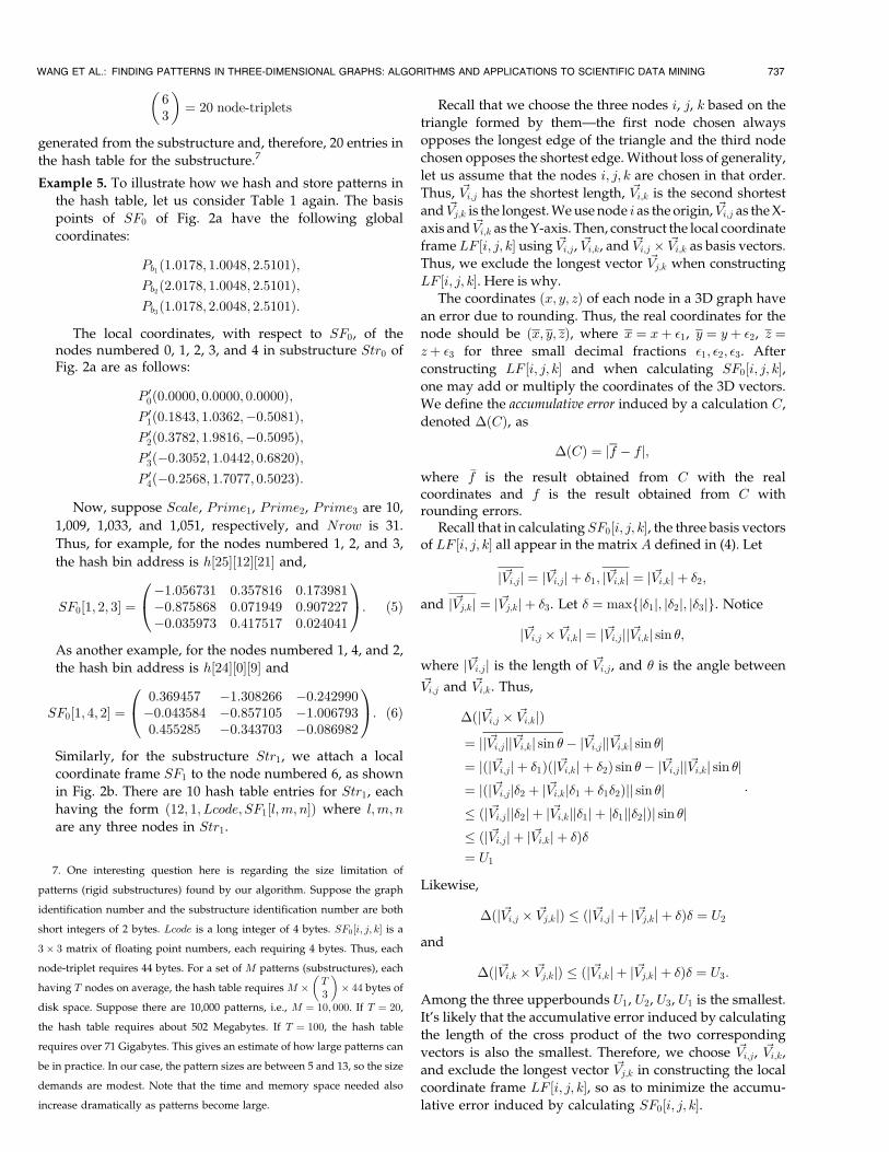
Example 5. To illustrate how we hash and store patterns in

the hash table, let us consider Table 1 again. The basis

points of SF0 of Fig. 2a have the following global

coordinates:

Pb1�1:0178; 1:0048; 2:5101�;

Pb2�2:0178; 1:0048; 2:5101�;

Pb3�1:0178; 2:0048; 2:5101�:

The local coordinates, with respect to SF0, of thenodes numbered 0, 1, 2, 3, and 4 in substructure Str0 ofFig. 2a are as follows:

P 00�0:0000; 0:0000; 0:0000�;P 01�0:1843; 1:0362;ÿ0:5081�;P 02�0:3782; 1:9816;ÿ0:5095�;P 03�ÿ0:3052; 1:0442; 0:6820�;P 04�ÿ0:2568; 1:7077; 0:5023�:

Now, suppose Scale, Prime1, Prime2, Prime3 are 10,

1,009, 1,033, and 1,051, respectively, and Nrow is 31.

Thus, for example, for the nodes numbered 1, 2, and 3,

the hash bin address is h�25��12��21� and,

SF0�1; 2; 3� �ÿ1:056731 0:357816 0:173981ÿ0:875868 0:071949 0:907227ÿ0:035973 0:417517 0:024041

0@ 1A: �5�

As another example, for the nodes numbered 1, 4, and 2,

the hash bin address is h�24��0��9� and

SF0�1; 4; 2� �0:369457 ÿ1:308266 ÿ0:242990ÿ0:043584 ÿ0:857105 ÿ1:0067930:455285 ÿ0:343703 ÿ0:086982

0@ 1A: �6�Similarly, for the substructure Str1, we attach a local

coordinate frame SF1 to the node numbered 6, as shown

in Fig. 2b. There are 10 hash table entries for Str1, each

having the form �12; 1; Lcode; SF1�l;m; n�� where l;m; n

are any three nodes in Str1.

Recall that we choose the three nodes i, j, k based on the

triangle formed by themÐthe first node chosen always

opposes the longest edge of the triangle and the third node

chosen opposes the shortest edge. Without loss of generality,

let us assume that the nodes i; j; k are chosen in that order.

Thus, ~Vi;j has the shortest length, ~Vi;k is the second shortest

and ~Vj;k is the longest. We use node i as the origin, ~Vi;j as the X-

axis and ~Vi;k as the Y-axis. Then, construct the local coordinate

frame LF �i; j; k� using ~Vi;j, ~Vi;k, and ~Vi;j � ~Vi;k as basis vectors.

Thus, we exclude the longest vector ~Vj;k when constructing

LF �i; j; k�. Here is why.The coordinates �x; y; z� of each node in a 3D graph have

an error due to rounding. Thus, the real coordinates for the

node should be �x; y; z�, where x � x� �1, y � y� �2, z �z� �3 for three small decimal fractions �1; �2; �3. After

constructing LF �i; j; k� and when calculating SF0�i; j; k�,one may add or multiply the coordinates of the 3D vectors.

We define the accumulative error induced by a calculation C,

denoted ��C�, as

��C� � jf ÿ fj;where �f is the result obtained from C with the realcoordinates and f is the result obtained from C withrounding errors.

Recall that in calculating SF0�i; j; k�, the three basis vectorsof LF �i; j; k� all appear in the matrix A defined in (4). Let

j~Vi;jj � j~Vi;jj � �1; j~Vi;kj � j~Vi;kj � �2;

and j~Vj;kj � j~Vj;kj � �3. Let � � maxfj�1j; j�2j; j�3jg. Notice

j~Vi;j � ~Vi;kj � j~Vi;jjj~Vi;kj sin �;

where j~Vi;jj is the length of ~Vi;j, and � is the angle between

~Vi;j and ~Vi;k. Thus,

��j~Vi;j � ~Vi;kj�� jj~Vi;jjj~Vi;kj sin �ÿ j~Vi;jjj~Vi;kj sin �j� j�j~Vi;jj � �1��j~Vi;kj � �2� sin �ÿ j~Vi;jjj~Vi;kj sin �j� j�j~Vi;jj�2 � j~Vi;kj�1 � �1�2�jj sin �j� �j~Vi;jjj�2j � j~Vi;kjj�1j � j�1jj�2j�j sin �j� �j~Vi;jj � j~Vi;kj � ���� U1

:

Likewise,

��j~Vi;j � ~Vj;kj� � �j~Vi;jj � j~Vj;kj � ��� � U2

and

��j~Vi;k � ~Vj;kj� � �j~Vi;kj � j~Vj;kj � ��� � U3:

Among the three upperbounds U1, U2, U3, U1 is the smallest.

It's likely that the accumulative error induced by calculating

the length of the cross product of the two corresponding

vectors is also the smallest. Therefore, we choose ~Vi;j, ~Vi;k,

and exclude the longest vector ~Vj;k in constructing the local

coordinate frame LF �i; j; k�, so as to minimize the accumu-

lative error induced by calculating SF0�i; j; k�.

WANG ET AL.: FINDING PATTERNS IN THREE-DIMENSIONAL GRAPHS: ALGORITHMS AND APPLICATIONS TO SCIENTIFIC DATA MINING 737

7. One interesting question here is regarding the size limitation of

patterns (rigid substructures) found by our algorithm. Suppose the graph

identification number and the substructure identification number are both

short integers of 2 bytes. Lcode is a long integer of 4 bytes. SF0�i; j; k� is a

3� 3 matrix of floating point numbers, each requiring 4 bytes. Thus, each

node-triplet requires 44 bytes. For a set of M patterns (substructures), each

having T nodes on average, the hash table requires M � T3

� �� 44 bytes of

disk space. Suppose there are 10,000 patterns, i.e., M � 10; 000. If T � 20,

the hash table requires about 502 Megabytes. If T � 100, the hash table

requires over 71 Gigabytes. This gives an estimate of how large patterns can

be in practice. In our case, the pattern sizes are between 5 and 13, so the size

demands are modest. Note that the time and memory space needed also

increase dramatically as patterns become large.

2.3.2 Subphase B of Phase 2

Let H be the resulting hash table obtained in subphase A ofphase 2 of the pattern-finding algorithm. In subphase B, wecalculate the occurrence number of each candidate patternP by rehashing the node-triplets of P into H. This way, weare able to match a node-triplet tri of P with a node-triplettri0 of another substructure (candidate pattern) P 0 stored insubphase A where tri and tri0 have the same hash binaddress. By counting the node-triplet matches, one can inferwhether P matches P 0 and, therefore, whether P occurs inthe graph from which P 0 is generated.

We associate each substructure with several counters,

which are created and updated as illustrated by the

following example. Suppose the two substructures (pat-

terns) of graph G with identification number 12 in Fig. 1

have already been stored in the hash tableH in subphase A.

Suppose i; j; k, are three nodes in the substructure Str0 of G.

Thus, for this node-triplet, its entry in the hash table is

�12; 0; Lcode; SF0�i; j; k��. Now, in subphase B, consider

another pattern P ; we hash the node-triplets of P using

the same hash function. Let u; v; w, be three nodes in P that

have the same hash bin address as i; j; k; that is, the node-

triplet �u; v; w� ªmatchesº the node-triplet �i; j; k�. If the

nodes u; v; w, geometrically match the nodes i; j; k respec-

tively, i.e., they have coinciding 3D coordinates after

rotations and translations, we call the node-triplet match a

true match; otherwise it is a false match. For a true match, let

SFP � SF0�i; j; k� �~Vu;v~Vu;w

~Vu;v � ~Vu;w

0B@1CA� Pu

PuPu

0@ 1A: �7�

This SFP contains the coordinates of the three basis points

of the Substructure Frame 0 (SF0) with respect to the global

coordinate frame in which the pattern P is given. We

compare the SFP with those already associated with the

substructure Str0 (initially none is associated with Str0). If

the SFP differs from the existing ones, a new counter is

created, whose value is initialized to 1, and the new counter

is assigned to the SFP . If the SFP is the ªsameº as an

existing one with counter value Cnt,8 and the code of the

label-triplet of nodes i, j, k; equals the code of the label-

triplet of nodes u, v, w, then Cnt is incremented by one. In

general, a substructure may be associated with several

different SFP s, each having a counter.We now present the theory supporting this algorithm.

Below, Theorem 1 establishes a criterion based on which

one can detect and eliminate a false match. Below,

Theorem 2 justifies the procedure of incrementing the

counter values.

Theorem 1. Let Pc1, Pc2

, and Pc3be the three basis points forming

the SFP defined in (7), where Pc1is the origin. ~Vc1;c2

, ~Vc1;c3,

and ~Vc1;c2� ~Vc1;c3

are orthonormal vectors if and only if the

nodes u, v, and w geometrically match the nodes i, j, and k,respectively.

Proof. (If) Let A be as defined in (4) and let

B �~Vu;v~Vu;w

~Vu;v � ~Vu;w

0B@1CA: �8�

Note that, if u, v, and w geometrically match i, j, and k,

respectively, then jBj � jAj, where jBj (jAj, respectively)

is the determinant of the matrix B (matrix A, respec-

tively). That is to say, jAÿ1jjBj � 1.From (3) and by the definition of the SFP in (7),

we have

SFP �~Vi;b1

~Vi;b2

~Vi;b3

0B@1CA�Aÿ1 �B�

PuPuPu

0@ 1A: �9�

Thus, the SFP basically transforms Pb1, Pb2

, and Pb3via

two translations and one rotation, where Pb1, Pb2

, and Pb3

are the basis points of the Substructure Frame 0 (SF0).

Since ~Vb1;b2, ~Vb1;b3

, and ~Vb1;b2� ~Vb1;b3

are orthonormal

vectors, and translations and rotations do not change

this property [27], we know that ~Vc1;c2, ~Vc1;c3

, and ~Vc1;c2�

~Vc1;c3are orthonormal vectors.

(Only if) If u, v, and w do not match i, j and kgeometrically while having the same hash bin address,then there would be distortion in the aforementionedtransformation. Consequently, ~Vc1;c2

, ~Vc1;c3, and ~Vc1;c2

�~Vc1;c3

would no longer be orthonormal vectors. tu

Theorem 2. If two true node-triplet matches yield the same SFPand the codes of the corresponding label-triplets are the same,then the two node-triplet matches are augmentable, i.e., theycan be combined to form a larger substructure match betweenP and Str0.

Proof. Since three nodes are enough to set the SFP at a fixed

position and direction, all the other nodes in P will have

definite coordinates under this SFP . When another node-

triplet match yielding the same SFP occurs, it means that

geometrically there is at least one more node match

between Str0 and P . If the codes of the corresponding

label-triplets are the same, it means that the labels of the

corresponding nodes are the same. Therefore, the two

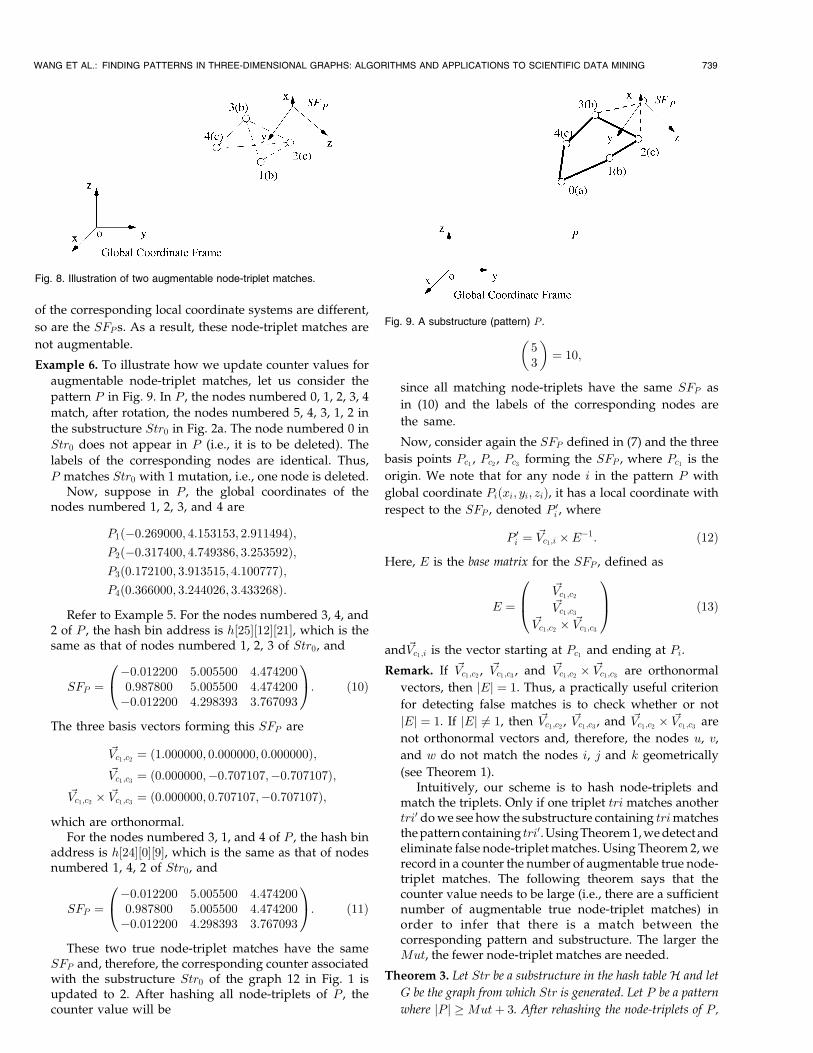
node-triplet matches are augmentable. tuFig. 8 illustrates how two node-triplet matches are

augmented. Suppose the node-triplet �3; 4; 2� yields the

SFP shown in the figure. Further, suppose that the node-

triplet �1; 2; 3� yields the same SFP , as shown in Fig. 8. Since

the labels of the corresponding nodes numbered 3 and 2 are

the same, we can augment the two node-triplets to form a

larger match containing nodes numbered 1, 2, 3, 4.Thus, by incrementing the counter associated with the

SFP , we record how many true node-triplet matches are

augmentable under this SFP . Notice that in cases where two

node-triplet matches occur due to reflections, the directions

738 IEEE TRANSACTIONS ON KNOWLEDGE AND DATA ENGINEERING, VOL. 14, NO. 4, JULY/AUGUST 2002

8. By saying SFP is the same as an existing SF 0P , we mean that for eachentry ei;j; 1 � i; j � 3, at the ith row and the jth column in SFP and itscorresponding entry e0i;j in SF 0P , jei;j ÿ e0i;jj � �, where � is an adjustableparameter depending on the data. In the examples presented in the paper,� � 0:01.

of the corresponding local coordinate systems are different,

so are the SFP s. As a result, these node-triplet matches are

not augmentable.

Example 6. To illustrate how we update counter values foraugmentable node-triplet matches, let us consider thepattern P in Fig. 9. In P , the nodes numbered 0, 1, 2, 3, 4

match, after rotation, the nodes numbered 5, 4, 3, 1, 2 inthe substructure Str0 in Fig. 2a. The node numbered 0 inStr0 does not appear in P (i.e., it is to be deleted). The

labels of the corresponding nodes are identical. Thus,P matches Str0 with 1 mutation, i.e., one node is deleted.

Now, suppose in P , the global coordinates of thenodes numbered 1, 2, 3, and 4 are

P1�ÿ0:269000; 4:153153; 2:911494�;P2�ÿ0:317400; 4:749386; 3:253592�;P3�0:172100; 3:913515; 4:100777�;P4�0:366000; 3:244026; 3:433268�:

Refer to Example 5. For the nodes numbered 3, 4, and2 of P , the hash bin address is h�25��12��21�, which is thesame as that of nodes numbered 1, 2, 3 of Str0, and

SFP �ÿ0:012200 5:005500 4:4742000:987800 5:005500 4:474200ÿ0:012200 4:298393 3:767093

0@ 1A: �10�

The three basis vectors forming this SFP are

~Vc1;c2� �1:000000; 0:000000; 0:000000�;

~Vc1;c3� �0:000000;ÿ0:707107;ÿ0:707107�;

~Vc1;c2� ~Vc1;c3

� �0:000000; 0:707107;ÿ0:707107�;which are orthonormal.

For the nodes numbered 3, 1, and 4 of P , the hash binaddress is h�24��0��9�, which is the same as that of nodesnumbered 1, 4, 2 of Str0, and

SFP �ÿ0:012200 5:005500 4:4742000:987800 5:005500 4:474200ÿ0:012200 4:298393 3:767093

0@ 1A: �11�

These two true node-triplet matches have the sameSFP and, therefore, the corresponding counter associatedwith the substructure Str0 of the graph 12 in Fig. 1 isupdated to 2. After hashing all node-triplets of P , thecounter value will be

53

� �� 10;

since all matching node-triplets have the same SFP as

in (10) and the labels of the corresponding nodes are

the same.

Now, consider again the SFP defined in (7) and the three

basis points Pc1, Pc2

, Pc3forming the SFP , where Pc1

is the

origin. We note that for any node i in the pattern P with

global coordinate Pi�xi; yi; zi�, it has a local coordinate with

respect to the SFP , denoted P 0i , where

P 0i � ~Vc1;i �Eÿ1: �12�Here, E is the base matrix for the SFP , defined as

E �~Vc1;c2

~Vc1;c3

~Vc1;c2� ~Vc1;c3

0B@1CA �13�

and~Vc1;i is the vector starting at Pc1and ending at Pi.

Remark. If ~Vc1;c2, ~Vc1;c3

, and ~Vc1;c2� ~Vc1;c3

are orthonormal

vectors, then jEj � 1. Thus, a practically useful criterion

for detecting false matches is to check whether or not

jEj � 1. If jEj 6� 1, then ~Vc1;c2, ~Vc1;c3

, and ~Vc1;c2� ~Vc1;c3

are

not orthonormal vectors and, therefore, the nodes u, v,

and w do not match the nodes i, j and k geometrically

(see Theorem 1).Intuitively, our scheme is to hash node-triplets and

match the triplets. Only if one triplet tri matches anothertri0 do we see how the substructure containing trimatchesthe pattern containing tri0. Using Theorem 1, we detect andeliminate false node-triplet matches. Using Theorem 2, werecord in a counter the number of augmentable true node-triplet matches. The following theorem says that thecounter value needs to be large (i.e., there are a sufficientnumber of augmentable true node-triplet matches) inorder to infer that there is a match between thecorresponding pattern and substructure. The larger theMut, the fewer node-triplet matches are needed.

Theorem 3. Let Str be a substructure in the hash table H and let

G be the graph from which Str is generated. Let P be a pattern

where jP j �Mut� 3. After rehashing the node-triplets of P ,

WANG ET AL.: FINDING PATTERNS IN THREE-DIMENSIONAL GRAPHS: ALGORITHMS AND APPLICATIONS TO SCIENTIFIC DATA MINING 739

Fig. 9. A substructure (pattern) P .

Fig. 8. Illustration of two augmentable node-triplet matches.

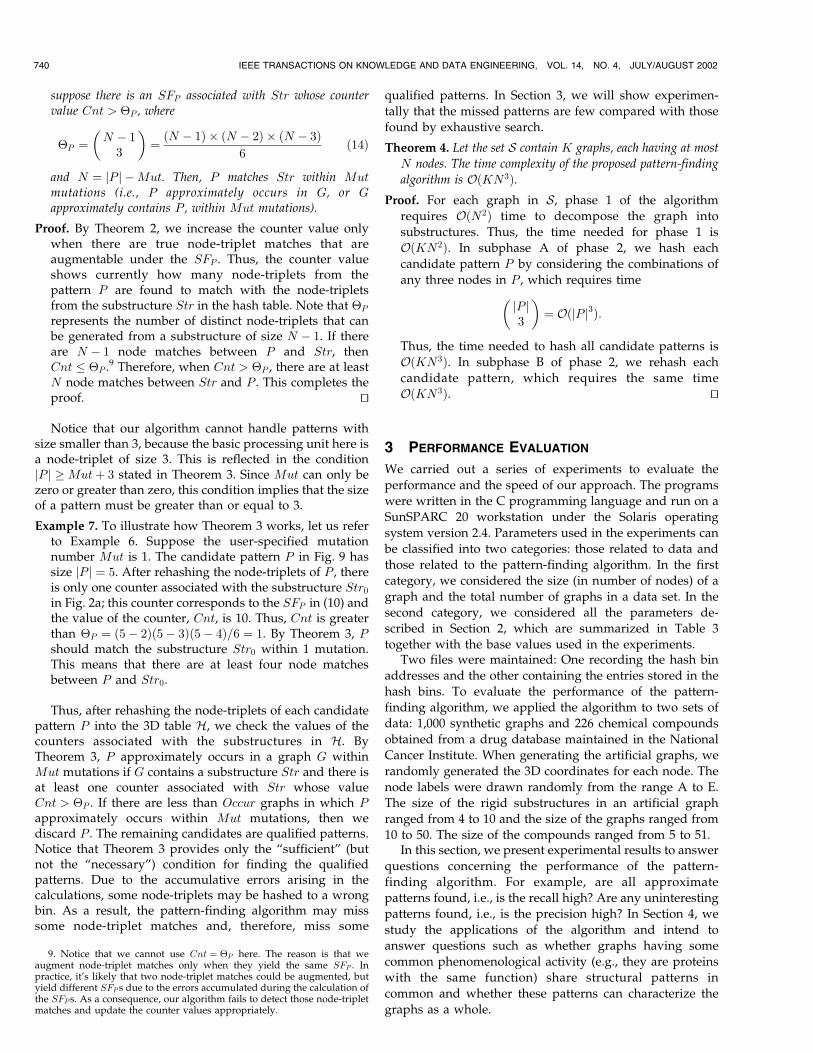
suppose there is an SFP associated with Str whose countervalue Cnt > �P , where

�P � N ÿ 13

� �� �N ÿ 1� � �N ÿ 2� � �N ÿ 3�

6�14�

and N � jP j ÿMut. Then, P matches Str within Mutmutations (i.e., P approximately occurs in G, or Gapproximately contains P , within Mut mutations).

Proof. By Theorem 2, we increase the counter value onlywhen there are true node-triplet matches that areaugmentable under the SFP . Thus, the counter valueshows currently how many node-triplets from thepattern P are found to match with the node-tripletsfrom the substructure Str in the hash table. Note that �P

represents the number of distinct node-triplets that canbe generated from a substructure of size N ÿ 1. If thereare N ÿ 1 node matches between P and Str, thenCnt � �P .9 Therefore, when Cnt > �P , there are at leastN node matches between Str and P . This completes theproof. tu

Notice that our algorithm cannot handle patterns withsize smaller than 3, because the basic processing unit here isa node-triplet of size 3. This is reflected in the conditionjP j �Mut� 3 stated in Theorem 3. Since Mut can only bezero or greater than zero, this condition implies that the sizeof a pattern must be greater than or equal to 3.

Example 7. To illustrate how Theorem 3 works, let us referto Example 6. Suppose the user-specified mutationnumber Mut is 1. The candidate pattern P in Fig. 9 hassize jP j � 5. After rehashing the node-triplets of P , thereis only one counter associated with the substructure Str0

in Fig. 2a; this counter corresponds to the SFP in (10) andthe value of the counter, Cnt, is 10. Thus, Cnt is greaterthan �P � �5ÿ 2��5ÿ 3��5ÿ 4�=6 � 1. By Theorem 3, Pshould match the substructure Str0 within 1 mutation.This means that there are at least four node matchesbetween P and Str0.

Thus, after rehashing the node-triplets of each candidatepattern P into the 3D table H, we check the values of thecounters associated with the substructures in H. ByTheorem 3, P approximately occurs in a graph G withinMut mutations if G contains a substructure Str and there isat least one counter associated with Str whose valueCnt > �P . If there are less than Occur graphs in which Papproximately occurs within Mut mutations, then wediscard P . The remaining candidates are qualified patterns.Notice that Theorem 3 provides only the ªsufficientº (butnot the ªnecessaryº) condition for finding the qualifiedpatterns. Due to the accumulative errors arising in thecalculations, some node-triplets may be hashed to a wrongbin. As a result, the pattern-finding algorithm may misssome node-triplet matches and, therefore, miss some

qualified patterns. In Section 3, we will show experimen-tally that the missed patterns are few compared with thosefound by exhaustive search.

Theorem 4. Let the set S contain K graphs, each having at most

N nodes. The time complexity of the proposed pattern-finding

algorithm is O�KN3�.Proof. For each graph in S, phase 1 of the algorithm

requires O�N2� time to decompose the graph intosubstructures. Thus, the time needed for phase 1 isO�KN2�. In subphase A of phase 2, we hash each

candidate pattern P by considering the combinations ofany three nodes in P , which requires time

jP j3

� �� O�jP j3�:

Thus, the time needed to hash all candidate patterns is

O�KN3�. In subphase B of phase 2, we rehash eachcandidate pattern, which requires the same timeO�KN3�. tu

3 PERFORMANCE EVALUATION

We carried out a series of experiments to evaluate the

performance and the speed of our approach. The programswere written in the C programming language and run on aSunSPARC 20 workstation under the Solaris operating

system version 2.4. Parameters used in the experiments canbe classified into two categories: those related to data andthose related to the pattern-finding algorithm. In the firstcategory, we considered the size (in number of nodes) of a

graph and the total number of graphs in a data set. In thesecond category, we considered all the parameters de-scribed in Section 2, which are summarized in Table 3together with the base values used in the experiments.

Two files were maintained: One recording the hash bin

addresses and the other containing the entries stored in thehash bins. To evaluate the performance of the pattern-finding algorithm, we applied the algorithm to two sets ofdata: 1,000 synthetic graphs and 226 chemical compounds

obtained from a drug database maintained in the NationalCancer Institute. When generating the artificial graphs, werandomly generated the 3D coordinates for each node. The

node labels were drawn randomly from the range A to E.The size of the rigid substructures in an artificial graphranged from 4 to 10 and the size of the graphs ranged from10 to 50. The size of the compounds ranged from 5 to 51.

In this section, we present experimental results to answer

questions concerning the performance of the pattern-finding algorithm. For example, are all approximatepatterns found, i.e., is the recall high? Are any uninterestingpatterns found, i.e., is the precision high? In Section 4, we

study the applications of the algorithm and intend toanswer questions such as whether graphs having somecommon phenomenological activity (e.g., they are proteinswith the same function) share structural patterns in

common and whether these patterns can characterize thegraphs as a whole.

740 IEEE TRANSACTIONS ON KNOWLEDGE AND DATA ENGINEERING, VOL. 14, NO. 4, JULY/AUGUST 2002

9. Notice that we cannot use Cnt � �P here. The reason is that weaugment node-triplet matches only when they yield the same SFP . Inpractice, it's likely that two node-triplet matches could be augmented, butyield different SFP s due to the errors accumulated during the calculation ofthe SFP s. As a consequence, our algorithm fails to detect those node-tripletmatches and update the counter values appropriately.

3.1 Effect of Data-Related Parameters

To evaluate the performance of the proposed pattern-

finding algorithm, we compared it with exhaustive search.

The exhaustive search procedure works by generating all

candidate patterns as in phase 1 of the pattern-finding

algorithm. Then, the procedure examines if a pattern P

approximately matches a substructure Str in a graph by

permuting the node labels of P and checking if they match

the node labels of Str. If so, the procedure performs

translation and rotation on P and checks if P can

geometrically match Str.The speed of the algorithms was measured by the

running time. The performance was evaluated using three

measures: recall (RE), precision (PR), and the number of

false matches, Nfm, arising during the hashing process.

(Recall that a false match arises, if a node-triplet �u; v; w�from a pattern P has the same hash bin address as a node-

triplet �i; j; k� from a substructure of graph G, though the

nodes u; v; w do not match the nodes i; j; k geometrically,

see Section 2.3.2.) Recall is defined as

RE � UPFoundTotalP

� 100%:

Precision is defined as

PR � UPFoundPFound

� 100%;

where PFound is the number of patterns found by the

proposed algorithm, UPFound is the number of patterns

found that satisfy the user-specified parameter values, and

TotalP is the number of qualified patterns found by

exhaustive search. One would like both RE and PR to be

as high as possible. Fig. 10 shows the running times of the

algorithms as a function of the number of graphs and Fig. 11

shows the recall. The parameters used in the proposed

pattern-finding algorithm had the values shown in Table 3.

As can be seen from the figures, the proposed algorithm is

10,000 times faster than the exhaustive search method when

the data set has more than 600 graphs while achieving a

very high (> 97%) recall. Due to the accumulative errors

arising in the calculations, some node-triplets may be

hashed to a wrong bin. As a result, the proposed algorithm

may miss some node-triplet matches in subphase B of

phase 2 and, therefore, cannot achieve a 100 percent recall.

In these experiments, precision was 100 percent.Fig. 12 shows the number of false matches introduced by

the proposed algorithm as a function of the number of

graphs. For the chemical compounds, Nfm is small. For the

synthetic graphs, Nfm increases as the number of graphs

WANG ET AL.: FINDING PATTERNS IN THREE-DIMENSIONAL GRAPHS: ALGORITHMS AND APPLICATIONS TO SCIENTIFIC DATA MINING 741

Fig. 10. Running times as a function of the number of graphs. Fig. 11. Recall as a function of the number of graphs.

TABLE 3Parameters in the Pattern-Finding Algorithm and Their Base Values Used in the Experiments

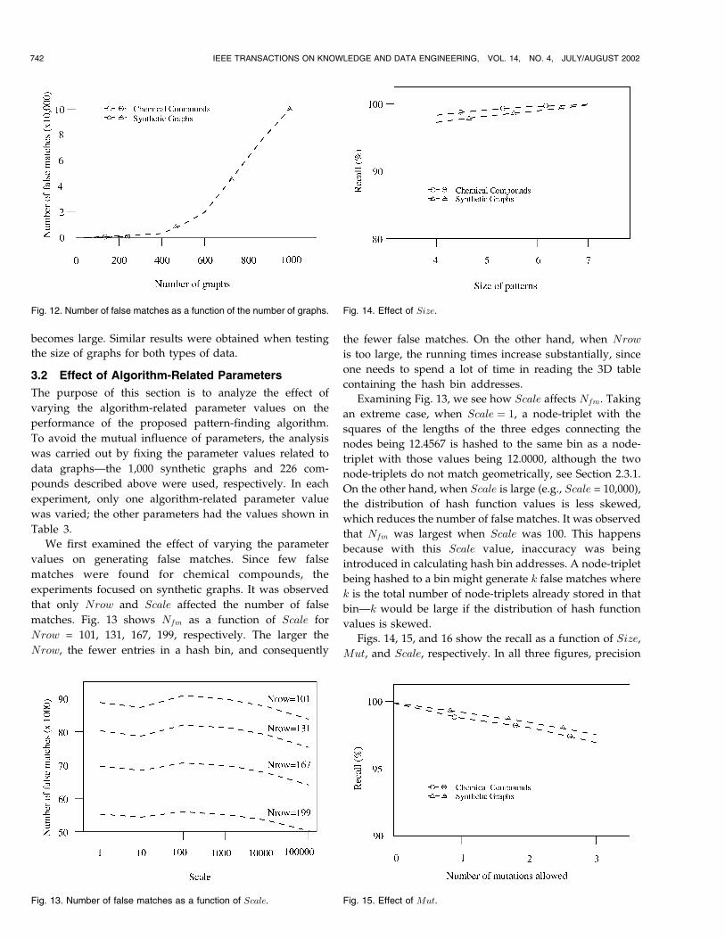
becomes large. Similar results were obtained when testing

the size of graphs for both types of data.

3.2 Effect of Algorithm-Related Parameters

The purpose of this section is to analyze the effect of

varying the algorithm-related parameter values on the

performance of the proposed pattern-finding algorithm.

To avoid the mutual influence of parameters, the analysis

was carried out by fixing the parameter values related to

data graphsÐthe 1,000 synthetic graphs and 226 com-

pounds described above were used, respectively. In each

experiment, only one algorithm-related parameter value

was varied; the other parameters had the values shown in

Table 3.

We first examined the effect of varying the parameter

values on generating false matches. Since few false

matches were found for chemical compounds, the

experiments focused on synthetic graphs. It was observed

that only Nrow and Scale affected the number of false

matches. Fig. 13 shows Nfm as a function of Scale for

Nrow = 101, 131, 167, 199, respectively. The larger the

Nrow, the fewer entries in a hash bin, and consequently

the fewer false matches. On the other hand, when Nrow

is too large, the running times increase substantially, since

one needs to spend a lot of time in reading the 3D table

containing the hash bin addresses.

Examining Fig. 13, we see how Scale affects Nfm. Taking

an extreme case, when Scale � 1, a node-triplet with the

squares of the lengths of the three edges connecting the

nodes being 12.4567 is hashed to the same bin as a node-

triplet with those values being 12.0000, although the two

node-triplets do not match geometrically, see Section 2.3.1.

On the other hand, when Scale is large (e.g., Scale = 10,000),

the distribution of hash function values is less skewed,

which reduces the number of false matches. It was observed

that Nfm was largest when Scale was 100. This happens

because with this Scale value, inaccuracy was being

introduced in calculating hash bin addresses. A node-triplet

being hashed to a bin might generate k false matches where

k is the total number of node-triplets already stored in that

binÐk would be large if the distribution of hash function

values is skewed.

Figs. 14, 15, and 16 show the recall as a function of Size,

Mut, and Scale, respectively. In all three figures, precision

742 IEEE TRANSACTIONS ON KNOWLEDGE AND DATA ENGINEERING, VOL. 14, NO. 4, JULY/AUGUST 2002

Fig. 12. Number of false matches as a function of the number of graphs.

Fig. 13. Number of false matches as a function of Scale.

Fig. 14. Effect of Size.

Fig. 15. Effect of Mut.

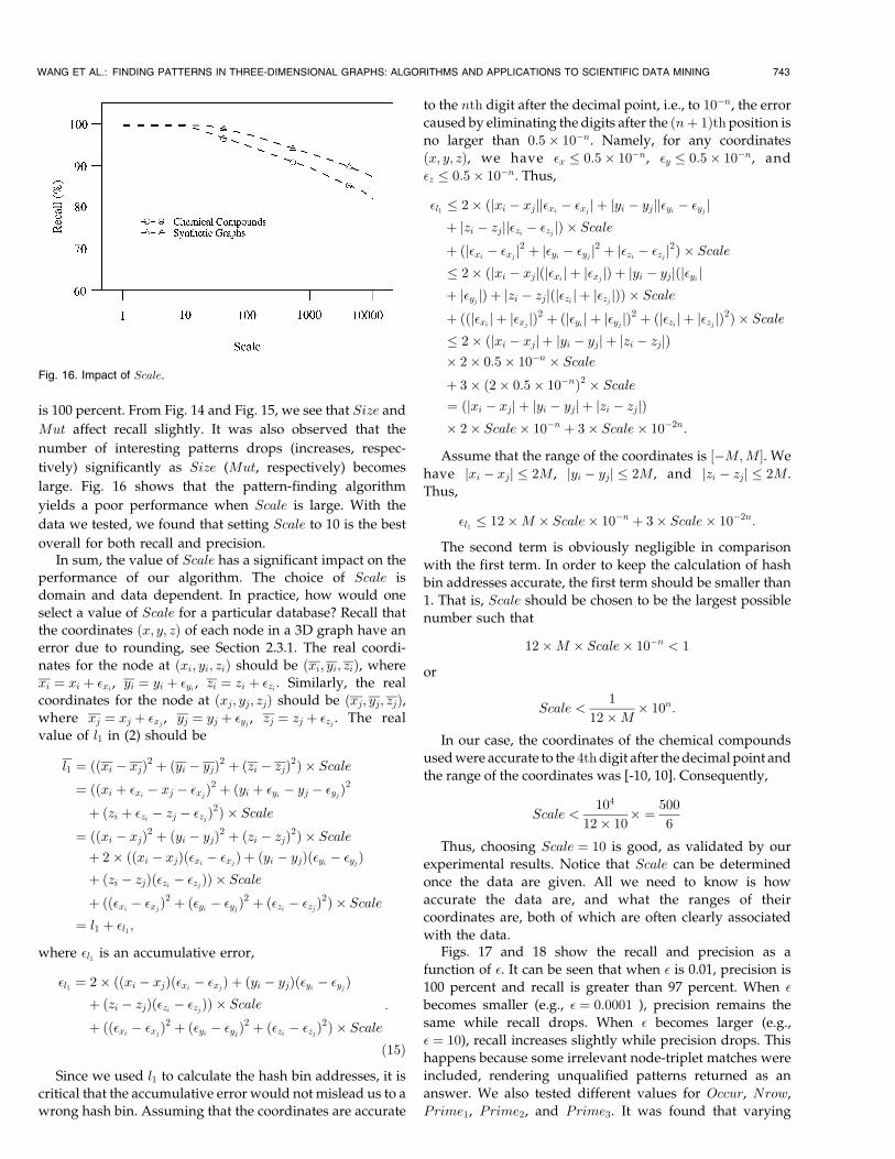
is 100 percent. From Fig. 14 and Fig. 15, we see that Size and

Mut affect recall slightly. It was also observed that the

number of interesting patterns drops (increases, respec-

tively) significantly as Size (Mut, respectively) becomes

large. Fig. 16 shows that the pattern-finding algorithm

yields a poor performance when Scale is large. With the

data we tested, we found that setting Scale to 10 is the best

overall for both recall and precision.In sum, the value of Scale has a significant impact on the

performance of our algorithm. The choice of Scale isdomain and data dependent. In practice, how would one

select a value of Scale for a particular database? Recall thatthe coordinates �x; y; z� of each node in a 3D graph have anerror due to rounding, see Section 2.3.1. The real coordi-

nates for the node at �xi; yi; zi� should be �xi; yi; zi�, wherexi � xi � �xi , yi � yi � �yi , zi � zi � �zi . Similarly, the realcoordinates for the node at �xj; yj; zj� should be �xj; yj; zj�,where xj � xj � �xj , yj � yj � �yj , zj � zj � �zj . The realvalue of l1 in (2) should be

l1 � ��xi ÿ xj�2 � �yi ÿ yj�2 � �zi ÿ zj�2� � Scale� ��xi � �xi ÿ xj ÿ �xj�2 � �yi � �yi ÿ yj ÿ �yj�2

� �zi � �zi ÿ zj ÿ �zj�2� � Scale� ��xi ÿ xj�2 � �yi ÿ yj�2 � �zi ÿ zj�2� � Scale� 2� ��xi ÿ xj���xi ÿ �xj� � �yi ÿ yj���yi ÿ �yj�� �zi ÿ zj���zi ÿ �zj�� � Scale� ���xi ÿ �xj�2 � ��yi ÿ �yj�2 � ��zi ÿ �zj�2� � Scale� l1 � �l1 ;

where �l1 is an accumulative error,

�l1 � 2� ��xi ÿ xj���xi ÿ �xj� � �yi ÿ yj���yi ÿ �yj�� �zi ÿ zj���zi ÿ �zj�� � Scale� ���xi ÿ �xj�2 � ��yi ÿ �yj�2 � ��zi ÿ �zj�2� � Scale

:

�15�Since we used l1 to calculate the hash bin addresses, it is

critical that the accumulative error would not mislead us to awrong hash bin. Assuming that the coordinates are accurate

to the nth digit after the decimal point, i.e., to 10ÿn, the error

caused by eliminating the digits after the �n� 1�th position is

no larger than 0:5� 10ÿn. Namely, for any coordinates

�x; y; z�, we have �x � 0:5� 10ÿn, �y � 0:5� 10ÿn, and

�z � 0:5� 10ÿn. Thus,

�l1 � 2� �jxi ÿ xjjj�xi ÿ �xj j � jyi ÿ yjjj�yi ÿ �yj j� jzi ÿ zjjj�zi ÿ �zj j� � Scale� �j�xi ÿ �xj j2 � j�yi ÿ �yj j2 � j�zi ÿ �zj j2� � Scale� 2� �jxi ÿ xjj�j�xi j � j�xj j� � jyi ÿ yjj�j�yi j� j�yj j� � jzi ÿ zjj�j�zi j � j�zj j�� � Scale� ��j�xi j � j�xj j�2 � �j�yi j � j�yj j�2 � �j�zi j � j�zj j�2� � Scale� 2� �jxi ÿ xjj � jyi ÿ yjj � jzi ÿ zjj�� 2� 0:5� 10ÿn � Scale� 3� �2� 0:5� 10ÿn�2 � Scale� �jxi ÿ xjj � jyi ÿ yjj � jzi ÿ zjj�� 2� Scale� 10ÿn � 3� Scale� 10ÿ2n:

Assume that the range of the coordinates is �ÿM;M�. We

have jxi ÿ xjj � 2M, jyi ÿ yjj � 2M, and jzi ÿ zjj � 2M.

Thus,

�l1 � 12�M � Scale� 10ÿn � 3� Scale� 10ÿ2n:

The second term is obviously negligible in comparison

with the first term. In order to keep the calculation of hash

bin addresses accurate, the first term should be smaller than

1. That is, Scale should be chosen to be the largest possible

number such that

12�M � Scale� 10ÿn < 1

or

Scale <1

12�M � 10n:

In our case, the coordinates of the chemical compounds

used were accurate to the 4th digit after the decimal point and

the range of the coordinates was [-10, 10]. Consequently,

Scale <104

12� 10� � 500

6

Thus, choosing Scale � 10 is good, as validated by our

experimental results. Notice that Scale can be determined

once the data are given. All we need to know is how

accurate the data are, and what the ranges of their

coordinates are, both of which are often clearly associated

with the data.Figs. 17 and 18 show the recall and precision as a

function of �. It can be seen that when � is 0.01, precision is

100 percent and recall is greater than 97 percent. When �

becomes smaller (e.g., � � 0:0001 ), precision remains the

same while recall drops. When � becomes larger (e.g.,

� � 10), recall increases slightly while precision drops. This

happens because some irrelevant node-triplet matches were

included, rendering unqualified patterns returned as an

answer. We also tested different values for Occur, Nrow,

Prime1, Prime2, and Prime3. It was found that varying

WANG ET AL.: FINDING PATTERNS IN THREE-DIMENSIONAL GRAPHS: ALGORITHMS AND APPLICATIONS TO SCIENTIFIC DATA MINING 743

Fig. 16. Impact of Scale.

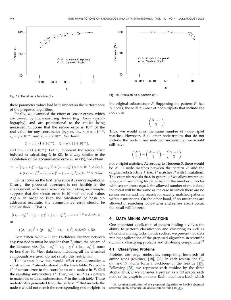
these parameter values had little impact on the performanceof the proposed algorithm.

Finally, we examined the effect of sensor errors, whichare caused by the measuring device (e.g., X-ray crystal-lography), and are proportional to the values beingmeasured. Suppose that the sensor error is 10ÿn of thereal value for any coordinates �x; y; z�, i.e., �x � x� 10ÿn,�y � y� 10ÿn, and �z � z� 10ÿn. We have

x � x� �1� 10ÿn�; y � y� �1� 10ÿn�;and z � z� �1� 10ÿn�. Let l1 represent the sensor errorinduced in calculating l1 in (2). In a way similar to thecalculation of the accumulative error �l1 in (15), we obtain

l1 ���xi ÿ xj�2 � �yi ÿ yj�2 � �zi ÿ zj�2� � 2� 10ÿn � Scale� ��xi ÿ xj�2 � �yi ÿ yj�2 � �zi ÿ zj�2� � 10ÿ2n � Scale:

Let us focus on the first term since it is more significant.Clearly, the proposed approach is not feasible in theenvironment with large sensor errors. Taking an example,suppose that the sensor error is 10ÿ2 of the real value.Again, in order to keep the calculation of hash binaddresses accurate, the accumulative error should besmaller than 1. That is,

��xi ÿ xj�2 � �yi ÿ yj�2 � �zi ÿ zj�2� � 2� 10ÿ2 � Scale < 1

or

��xi ÿ xj�2 � �yi ÿ yj�2 � �zi ÿ zj�2� � Scale < 50:

Even when Scale � 1, the Euclidean distance between

any two nodes must be smaller than 7, since the square of

the distance, viz. ��xi ÿ xj�2 � �yi ÿ yj�2 � �zi ÿ zj�2�, must

be less than 50. Most data sets, including all the chemical

compounds we used, do not satisfy this restriction.To illustrate how this would affect recall, consider a

substructure P already stored in the hash table. We add a10ÿ2 sensor error to the coordinates of a node v in P . Callthe resulting substructure P 0. Then, we use P 0 as a patternto match the original substructure P in the hash table. Thosenode-triplets generated from the pattern P 0 that include thenode v would not match the corresponding node-triplets in

the original substructure P . Supposing the pattern P 0 hasN nodes, the total number of node-triplets that include thenode v is

N ÿ 12

� �:

Thus, we would miss the same number of node-tripletmatches. However, if all other node-triplets that do notinclude the node v are matched successfully, we wouldstill have

N3

� �ÿ N ÿ 1

2

� �� N ÿ 1

3

� �node-triplet matches. According to Theorem 3, there wouldbe N ÿ 1 node matches between the pattern P 0 and theoriginal substructure P (i.e., P 0 matches P with 1 mutation).This example reveals that, in general, if we allow mutationsto occur in searching for patterns and the number of nodeswith sensor errors equals the allowed number of mutations,the recall will be the same as the case in which there are nosensor errors and we search for exactly matched patternswithout mutations. On the other hand, if no mutations areallowed in searching for patterns and sensor errors occur,the recall will be zero.

4 DATA MINING APPLICATIONS

One important application of pattern finding involves theability to perform classification and clustering as well asother data mining tasks. In this section, we present two datamining applications of the proposed algorithm in scientificdomains: classifying proteins and clustering compounds.10

4.1 Classifying Proteins

Proteins are large molecules, comprising hundreds ofamino acids (residues) [18], [33]. In each residue the C�,C�, and N atoms form a backbone of the residue [17].Following [28], we represent each residue by the threeatoms. Thus, if we consider a protein as a 3D graph, eachnode of the graph is an atom. Each node has a label, which

744 IEEE TRANSACTIONS ON KNOWLEDGE AND DATA ENGINEERING, VOL. 14, NO. 4, JULY/AUGUST 2002

Fig. 18. Precision as a function of �.

10. Another application of the proposed algorithm to flexible chemicalsearching in 3D structural databases can be found in [34].

Fig. 17. Recall as a function of �.

is the name of the atom and is not unique in the protein. Weassign a unique number to identify a node in the protein,where the order of numbering is obtained from the ProteinData Bank (PDB) [1], [2], accessible at http://www.rcsb.org.

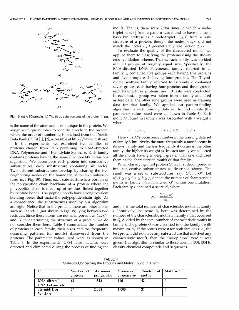
In the experiments, we examined two families ofproteins chosen from PDB pertaining to RNA-directedDNA Polymerase and Thymidylate Synthase. Each familycontains proteins having the same functionality in variousorganisms. We decompose each protein into consecutivesubstructures, each substructure containing six nodes.Two adjacent substructures overlap by sharing the twoneighboring nodes on the boundary of the two substruc-tures (see Fig. 19). Thus, each substructure is a portion ofthe polypeptide chain backbone of a protein where thepolypeptide chain is made up of residues linked togetherby peptide bonds. The peptide bonds have strong covalentbonding forces that make the polypeptide chain rigid. Asa consequence, the substructures used by our algorithmare rigid. Notice that in the proteins there are other atomssuch as O and H (not shown in Fig. 19) lying between tworesidues. Since these atoms are not as important as C�, C�,and N in determining the structure of a protein, we donot consider them here. Table 4 summarizes the numberof proteins in each family, their sizes and the frequentlyoccurring patterns (or motifs) discovered from theproteins. The parameter values used were as shown inTable 3. In the experiments, 2,784 false matches weredetected and eliminated during the process of finding the

motifs. That is, there were 2,784 times in which a node-triplet �u; v; w� from a pattern was found to have the samehash bin address as a node-triplet �i; j; k� from a sub-structure of a protein, though the nodes u; v; w did notmatch the nodes i; j; k geometrically, see Section 2.3.2.

To evaluate the quality of the discovered motifs, weapplied them to classifying the proteins using the 10-waycross-validation scheme. That is, each family was dividedinto 10 groups of roughly equal size. Specifically, theRNA-directed DNA Polymerase family, referred to asfamily 1, contained five groups each having five proteinsand five groups each having four proteins. The Thymi-dylate Synthase family, referred to as family 2, containedseven groups each having four proteins and three groupseach having three proteins, and 10 tests were conducted.In each test, a group was taken from a family and usedas test data; the other nine groups were used as trainingdata for that family. We applied our pattern-findingalgorithm to each training data set to find motifs (theparameter values used were as shown in Table 3). Eachmotif M found in family i was associated with a weight dwhere

d � ri ÿ rj 1 � i; j � 2; i 6� j:Here ri is M's occurrence number in the training data set

of family i. Intuitively, the more frequently a motif occurs inits own family and the less frequently it occurs in the otherfamily, the higher its weight is. In each family we collectedall the motifs having a weight greater than one and usedthem as the characteristic motifs of that family.

When classifying a test protein Q, we first decomposed Qinto consecutive substructures as described above. Theresult was a set of substructures, say, Q1; . . . ; Qp. Letnki ; 1 � i � 2; 1 � k � p, denote the number of characteristicmotifs in family i that matched Qk within one mutation.Each family i obtained a score Ni where

Ni �Pp

k�1 nki

mi

and mi is the total number of characteristic motifs in familyi. Intuitively, the score Ni here was determined by thenumber of the characteristic motifs in family i that occurredin Q, divided by the total number of characteristic motifs infamily i. The protein Q was classified into the family i withmaximum Ni. If the scores were 0 for both families (i.e., thetest protein did not have any substructure that matched anycharacteristic motif), then the ªno-opinionº verdict wasgiven. This algorithm is similar to those used in [30], [35] toclassify chemical compounds and sequences.

WANG ET AL.: FINDING PATTERNS IN THREE-DIMENSIONAL GRAPHS: ALGORITHMS AND APPLICATIONS TO SCIENTIFIC DATA MINING 745

Fig. 19. (a) A 3D protein. (b) The three substructures of the protein in (a).

TABLE 4Statistics Concerning the Proteins and Motifs Found in Them

As in Section 3, we use recall (REc) and precision (PRc)to evaluate the effectiveness of our classification algorithm.Recall is defined as

REc � TotalNumÿP2

i�1 NumLossic

TotalNum� 100%;

where TotalNum is the total number of test proteins andNumLossic is the number of test proteins that belong tofamily i but are not assigned to family i by our algorithm(they are either assigned to family j, j 6� i, or they receivethe ªno-opinionº verdict). Precision is defined as

PRc � TotalNumÿP2

i�1 NumGainic

TotalNum� 100%;

where NumGainic is the number of test proteins that do notbelong to family i but are assigned by our algorithm tofamily i. With the 10-way cross validation scheme, theaverage REc over the 10 tests was 92.7 percent and theaverage PRc was 96.4 percent. It was found that 3.7 percenttest proteins on average received the ªno-opinionº verdictduring the classification. We repeated the same experimentsusing other parameter values and obtained similar results,except that larger Mut values (e.g., 3) generally yieldedlower REc.

The binary classification problem studied here is con-cerned with assigning a protein to one of two families. Thisproblem arises frequently in protein homology detection[31]. The performance of our technique degrades whenapplied to the n-ary classification problem, which isconcerned with assigning a protein to one of many families[32]. For example, we applied the technique to classifyingthree families of proteins and the REc and PRc dropped to80 percent.

4.2 Clustering Compounds

In addition to classifying proteins, we have developed analgorithm for clustering 3D graphs based on the patternsoccurring in the graphs and have applied the algorithmto grouping compounds. Given a collection S of 3Dgraphs, the algorithm first uses the procedure depicted inSection 2.2 to decompose the graphs into rigid substruc-tures. Let fStrpjp � 0; 1; :::; N ÿ 1g be the set of substruc-tures found in the graphs in S where jStrpj � Size.Using the proposed pattern-finding algorithm, we exam-ine each graph Gq in S and determine whether eachsubstructure Strp approximately occurs in Gq withinMut mutations. Each graph Gq is represented as a bitstring of length N , i.e., Gq � �b0

q ; b1q ; :::; b

Nÿ1q �, where

bpq �1 if Strp occurs in Gq within Mut mutations0 otherwise:

�For example, consider the two patterns P1 and P2 in

Fig. 3 and the three graphs in Fig. 3a. Suppose theallowed number of mutations is 0. Then, G1 is repre-sented as 10, G2 as 01, and G3 as 10. On the other hand,suppose the allowed number of mutations is 1. Then, G1

and G3 are represented as 11 and G2 as 01.The distance between two graphs Gx and Gy, denoted

d�Gx;Gy�, is defined as the Hamming distance [12] betweentheir bit strings. The algorithm then uses the well-known

average-group method [13] to cluster the graphs in S, whichworks as follows.

Initially, every graph is a cluster. The algorithm mergestwo nearest clusters to form a new cluster, until there areonly K clusters left where K is a user-specified parameter.The distance between two clusters C1 and C2 is given by

1

jC1jjC2jX

Gx2C1;Gy2C2

jd�Gx;Gy�j; �16�

where jCij, i � 1; 2, is the size of cluster Ci. The algorithmrequires O�N2� distance calculations where N is the totalnumber of graphs in S.

We applied this algorithm to clustering chemicalcompounds. Ninety eight compounds were chosen fromthe Merck Index that belonged to three groups pertaining toaromatic, bicyclicalkanes and photosynthesis. The data wascreated by the CORINA program that converted 2D data(represented in SMILES string) to 3D data (represented inPDB format) [22]. Table 5 lists the number of compounds ineach group, their sizes and the patterns discovered fromthem. The parameter values used were Size � 5, Occur � 1,Mut � 2; the other parameters had the values shown inTable 3.

To evaluate the effectiveness of our clustering algorithm,we applied it to finding clusters in the compounds. Theparameter value K was set to 3, as there were three groups.As in the previous sections, we use recall (REr) andprecision (PRr) to evaluate the effectiveness of the cluster-ing algorithm. Recall is defined as

REr � TotalNumÿPK

i�1 NumLossir

TotalNum� 100%;

where NumLossir is the number of compounds that belongto group Gi, but are assigned by our algorithm to group Gj,i 6� j, and TotalNum is the total number of compoundstested. Precision is defined as

PRr � TotalNumÿPK

i�1 NumGainir

TotalNum� 100%;

where NumGainir is the number of compounds that donot belong to group Gi, but are assigned by ouralgorithm to group Gi. Our experimental results indicatedthat REr � PRr � 99%. Out of the 98 compounds, onlyone compound in the photosynthesis group was assignedincorrectly to the bicyclicalkanes group. We experimentedwith other parameter values and obtained similarresults.11

5 RELATED WORK

There are several groups working on pattern finding (orknowledge discovery) in molecules and graphs. Conklin et al.[4], [5], [6], for example, represented a molecular structure asan image, which comprised a set of parts with their 3Dcoordinates and a set of relations that were preserved for theimage. The authors used an incremental, divisive approach todiscover the ªknowledgeº from a data set, that is, to build a

746 IEEE TRANSACTIONS ON KNOWLEDGE AND DATA ENGINEERING, VOL. 14, NO. 4, JULY/AUGUST 2002

11. The Occur value was fixed at 1 in these experiments because of thefact that all the compounds were represented as binary bit strings.

subsumption hierarchy that summarized and classified thedata set. The algorithm relied on a measure of similarityamong molecular images that was defined in terms of theirlargest common subimages. In [8], Djoko et al. developed asystem, called SUBDUE, that utilized the minimum descrip-tion length principle to find repeatedly occurring substruc-tures in a graph. Once a substructure was found, thesubstructure was used to simplify the graph by replacinginstances of the substructure with a pointer to thediscovered substructure. In [7], Dehaspe et al. usedDATALOG to represent compounds and applied datamining techniques to predicting chemical carcinogenicity.Their techniques were based on Mannila and Toivonen'salgorithm [15] for finding interesting patterns from a classof sentences in a database.

In contrast to the above work, we use the geometrichashing technique to find approximately common pat-terns in a set of 3D graphs without prior knowledge oftheir structures, positions, or occurrence frequency. Thegeometric hashing technique used here originated fromthe work of Lamdan and Wolfson for model basedrecognition in computer vision [14]. Several researchersattempted to parallelize the technique based on variousarchitectures, such as the Hypercube and the ConnectionMachine [3], [19], [20]. It was observed that the distribu-tion of the hash table entries might be skewed. To balancethe distribution of the hash function values, delicaterehash functions were designed [20]. There were alsoefforts exploring the uncertainty existing in the geometrichashing algorithms [11], [26].

In 1996, Rigoutsos et al. employed geometric hashing

and magic vectors for substructure matching in a database

of chemical compounds [21]. The magic vectors were bonds

among atoms; the choice of them was domain dependent

and was based on the type of each individual graph. We

extend the work in [21] by providing a framework for

discovering approximately common substructures in a set

of 3D graphs, and applying our techniques to both

compounds and proteins. Our approach differs from [21]

in that instead of using the magic vectors, we store a

coordinate system in a hash table entry. Furthermore, we

establish a theory for detecting and eliminating false

matches occurring in the hashing.More recently, Wolfson and his colleagues also applied

geometric hashing algorithms to protein docking and

recognition [23], [24], [29]. They attached a reference frame

to each substructure, where the reference frame is an

orthonormal coordinate frame of arbitrary orientations,

established at a ªhingeº point. This hinge point can be any

point or a specific point chosen based on chemical

considerations. The 3D substructure can be rotated around

the hinge point. The authors then developed schemes to

generate node-triplets and hash table indices. However,

based on those schemes, false matches cannot be detected in

the hash table and must be processed in a subsequent,

additional verification phase. Thus, even if a pattern

appears to match several substructures during the search-

ing phase, one has to compare the pattern with those

substructures one by one to make sure they are true

matches during the verification phase. When mutations are

allowed, which were not considered in [23], [24], [29], a

brute-force verification test would be very time-consuming.

For example, in comparing our approach with their

approach in performing protein classification as described

in Section 4, we found that both approaches yield the same

recall and precision, though our approach is 10 times faster

than their approach.

6 CONCLUSION

In this paper, we have presented an algorithm for findingpatterns in 3D graphs. A pattern here is a rigid substructurethat may occur in a graph after allowing for an arbitrarynumber of rotations and translations as well as a smallnumber of edit operations in the pattern or in the graph. Weused the algorithm to find approximately common patternsin a set of synthetic graphs, chemical compounds andproteins. This yields a kind of alphabet of patterns. Ourexperimental results demonstrated the good performance ofthe proposed algorithm and its usefulness for patterndiscovery. We then developed classification and clusteringalgorithms using the patterns found in the graphs, andapplied them to classifying proteins and clustering com-pounds. Empirical study showed high recall and precisionrates for both classification and clustering, indicating thesignificance of the patterns.

We have implemented the techniques presented in thepaper and are combining them with the algorithms foracyclic graph matching [36] into a toolkit. We use the toolkitto find patterns in various types of graphs arising indifferent domains and as part of our tree and graph searchengine project. The toolkit can be obtained from the authorsand is also accessible at http://www.cis.njit.edu/~jason/sigmod.html on the Web.

In the future, we plan to study topological graphmatching problems. One weakness of the proposed geo-metric hashing approach is its sensitivity to errors as wediscussed in Section 3.2. One has to tune the Scale

WANG ET AL.: FINDING PATTERNS IN THREE-DIMENSIONAL GRAPHS: ALGORITHMS AND APPLICATIONS TO SCIENTIFIC DATA MINING 747

TABLE 5Statistics Concerning the Chemical Compounds and Patterns Found in Them

parameter when the accuracy of data changes. Anotherweakness is that the geometric hashing approach doesn'ttake edges into consideration. In some domains, edges areimportant despite the nodes matching. For example, incomputer vision, edges may represent some kind ofboundaries and have to be considered in object recognition.(Notice that when applying the proposed geometrichashing approach to this domain, the node label alphabetcould be extended to contain semantic information, such ascolor, shape, etc.) We have done preliminary work intopological graph matching, in which our algorithmmatches edge distances and the software is accessible athttp://cs.nyu.edu/cs/faculty/shasha/papers/agm.html.We plan to combine geometric matching and topologicalmatching approaches to finding patterns in more general

graphs.

ACKNOWLEDGMENTS

The authors would like to thank the anonymous reviewersfor their constructive suggestions that helped improve boththe quality and the presentation of this paper. We alsothank Dr. Carol Venanzi, Bo Chen, and Song Peng for usefuldiscussions and for providing chemical compounds used inthe paper. This work was supported in part by US NationalScience Foundation grants IRI-9531548, IRI-9531554, IIS-9988345, IIS-9988636, and by the Natural Sciences andEngineering Research Council of Canada under Grant No.OGP0046373. Part of this work was done while X. Wangwas with the Department of Computer and InformationScience, New Jersey Institute of Technology. Part of thiswork was done while J.T.L. Wang was visiting CourantInstitute of Mathematical Sciences, New York University.

REFERENCES

[1] E.E. Abola, F.C. Bernstein, S.H. Bryant, T.F. Koetzle, and J. Weng,ªProtein Data Bank,º Data Comm. Int'l Union of Crystallography,pp. 107-132, 1987.

[2] F.C. Bernstein, T.F. Koetzle, G.J.B. Williams, E.F. Meyer, M.D.Brice, J.R. Rodgers, O. Kennard, T. Shimanouchi, and M. Tasumi,ªThe Protein Data Bank: A Computer-Based Archival File forMacromolecular Structures,º J. Molecular Biology, vol. 112, 1977.

[3] O. Bourdon and G. Medioni, ªObject Recognition Using Geo-metric Hashing on the Connection Machine,º Proc. 10th Int'l Conf.Pattern Recognition, pp. 596-600, 1990.

[4] D. Conklin, ªKnowledge Discovery in Molecular StructureDatabases,º doctoral dissertation, Dept. Computing and Informa-tion Science, Queen's Univ., Canada, 1995.

[5] D. Conklin, ªMachine Discovery of Protein Motifs,º MachineLearning, vol. 21, pp. 125-150, 1995.

[6] D. Conklin, S. Fortier, and J. Glasgow, ªKnowledge Discovery inMolecular Databases,º IEEE Trans. Knowledge and Data Eng., vol. 5,no. 6, pp. 985-987, 1993.

[7] L. Dehaspe, H. Toivonen, and R.D. King, ªFinding FrequentSubstructures in Chemical Compounds,º Proc. Fourth Int'l Conf.Knowledge Discovery and Data Mining, pp. 30-36, 1998.

[8] S. Djoko, D.J. Cook, and L.B. Holder, ªAn Empirical Study ofDomain Knowledge and Its Benefits to Substructure Discovery,ºIEEE Trans. Knowledge and Data Eng., vol. 9, no. 4, pp. 575-586,1997.

[9] D. Fischer, O. Bachar, R. Nussinov, and H.J. Wolfson, ªAnEfficient Automated Computer Vision Based Technique forDetection of Three Dimensional Structural Motifs in Proteins,ºJ. Biomolecular and Structural Dynamics, vol. 9, no. 4, pp. 769-789,1992.

[10] H.N. Gabow, Z. Galil, and T.H. Spencer, ªEfficient Implementa-tion of Graph Algorithms Using Contraction,º Proc. 25th Ann.IEEE Symp. Foundations of Computer Science, pp. 347-357, 1984.

[11] W.E.L. Grimson, D.P. Huttenlocher, and D.W. Jacobs, ªAffineMatching with Bounded Sensor Error: Study of GeometricHashing and Alignment,º Technical Memo AIM-1250, ArtificialIntelligence Laboratory, Massachusetts Inst. of Technology, 1991.

[12] R.W. Hamming ªError Detecting and Error Correcting Codes,ºThe Bell System Technical J., vol. 29, no. 2, pp. 147-160, 1950,Reprinted in E.E. Swartzlander, Computer Arithmetic. vol. 2, LosAlamitos, Calif.: IEEE Computer Soc. Press Tutorial, 1990.

[13] L. Kaufman and P.J. Rousseeuw, Finding Groups in Data: AnIntroduction to Cluster Analysis. New York: John Wiley & Sons,1990.

[14] Y. Lamdan and H. Wolfson, ªGeometric Hashing: A General andEfficient Model-Based Recognition Scheme,º Proc. Int'l Conf.Computer Vision, pp. 237-249, 1988.

[15] H. Mannila and H. Toivonen, ªLevelwise Search and Borders ofTheories in Knowledge Discovery,º Data Mining and KnowledgeDiscovery, vol. 1, no. 3, pp. 241-258, 1997.

[16] J.A. McHugh, Algorithmic Graph Theory. Englewood Cliffs, N.J.:Prentice Hall, 1990.

[17] X. Pennec and N. Ayache, ªAn O�n2� Algorithm for 3DSubstructure Matching of Proteins,º Proc. First Int'l WorkshopShape and Pattern Matching in Computational Biology, pp. 25-40,1994.

[18] C. Pu, K.P. Sheka, L. Chang, J. Ong, A. Chang, E. Alessio,I.N. Shindyalov, W. Chang, and P.E. Bourne, ªPDBtool: APrototype Object Oriented Toolkit for Protein StructureVerification,º Technical Report CUCS-048-92, Dept. ComputerScience, Columbia Univ., 1992.

[19] I. Rigoutsos and R. Hummel, ªScalable Parallel GeometricHashing for Hypercube (SIMD) Architectures,º Technical ReportTR-553, Dept. Computer Science, New York Univ., 1991.

[20] I. Rigoutsos and R. Hummel, ªOn a Parallel Implementation ofGeometric Hashing on the Connection Machine,º TechnicalReport TR-554, Dept. Computer Science, New York Univ., 1991.

[21] I. Rigoutsos, D. Platt, and A. Califano, ªFlexible SubstructureMatching in Very Large Databases of 3D-Molecular Information,ºresearch report, IBM T.J. Watson Research Center, YorktownHeights, N.Y., 1996.

[22] J. Sadowski and J. Gasteiger, ªFrom Atoms and Bonds to Three-Dimensional Atomic Coordinates: Automatic Model Builders,ºChemical Rev., pp. 2567-2581, vol. 93, 1993.

[23] B. Sandak, R. Nussinov, and H.J. Wolfson, ªA Method forBiomolecular Structural Recognition and Docking AllowingConformational Flexibility,º J. Computational Biology, vol. 5, no. 4,pp. 631-654, 1998.

[24] B. Sandak, H.J. Wolfson, and R. Nussinov, ªFlexible DockingAllowing Induced Fit in Proteins: Insights from an Open to ClosedConformational Isomers,º Proteins, vol. 32, pp. 159-74, 1998.

[25] Time Warps, String Edits, and Macromolecules: The Theory andPractice of Sequence Comparison. D. Sankoff and J.B. Kruskal, eds.,Reading, Mass.: Addison-Wesley, 1983.

[26] K.B. Sarachik, ªLimitations of Geometric Hashing in the Presenceof Gaussian Noise,º Technical Memo AIM-1395, Artificial Intelli-gence Laboratory, Massachusetts Inst. of Technology, 1992.

[27] R.R. Stoll, Linear Algebra and Matrix Theory, New York: McGraw-Hill, 1952.

[28] I.I. Vaisman, A. Tropsha, and W. Zheng, ªCompositionalPreferences in Quadruplets of Nearest Neighbor Residues inProtein Structures: Statistical Geometry Analysis,º Proc. IEEE Int'lJoin Symp. Intelligence and Systems, pp. 163-168, 1998.

[29] G. Verbitsky, R. Nussinov, and H.J. Wolfson, ªFlexible StructuralComparison Allowing Hinge Bending and Swiveling Motions,ºProteins, vol. 34, pp. 232-254, 1999.

[30] J.T.L. Wang, G.-W. Chirn, T.G. Marr, B.A. Shapiro, D. Shasha, andK. Zhang, ªCombinatorial Pattern Discovery for Scientific Data:Some Preliminary Results,º Proc. 1994 ACM SIGMOD Int'l Conf.Management of Data, pp. 115-125, 1994.

[31] J.T.L. Wang, Q. Ma, D. Shasha, and C.H. Wu, ªApplication ofNeural Networks to Biological Data Mining: A Case Study inProtein Sequence Classification,º Proc. Sixth ACM SIGKDD Int'lConf. Knowledge Discovery and Data Mining, pp. 305±309, 2000.

[32] J.T.L. Wang, T.G. Marr, D. Shasha, B. A. Shapiro, G.-W. Chirn, andT.Y. Lee, ªComplementary Classification Approaches for ProteinSequences,º Protein Eng., vol. 9, no. 5, pp. 381-386, 1996.

748 IEEE TRANSACTIONS ON KNOWLEDGE AND DATA ENGINEERING, VOL. 14, NO. 4, JULY/AUGUST 2002

[33] J.T.L. Wang, B.A. Shapiro, and D. Shasha, eds., Pattern Discovery inBiomolecular Data: Tools, Techniques and Applications, New York:Oxford Univ. Press, 1999.

[34] X. Wang and J.T.L. Wang, ªFast Similarity Search in Three-Dimensional Structure Databases,º J. Chemical Information andComputer Sciences, vol. 40, no. 2, pp. 442-451, 2000.

[35] X. Wang, J.T.L. Wang, D. Shasha, B.A. Shapiro, S. Dikshitulu,I. Rigoutsos, and K. Zhang, ªAutomated Discovery of ActiveMotifs in Three Dimensional Molecules,º Proc. Third Int'l Conf.Knowledge Discovery and Data Mining, pp. 89-95, 1997.

[36] K. Zhang, J.T.L. Wang, and D. Shasha, ªOn the Editing DistanceBetween Undirected Acyclic Graphs,º Int'l J. Foundations ofComputer Science, special issue on Computational Biology, vol. 7,no. 1, pp. 43-57, 1996.

Xiong Wang received the MS degree incomputer science from Fudan University, China,and the PhD degree in computer and informationscience from the New Jersey Institute ofTechnology, in 2000 ( thesis advisor :Jason T.L. Wang). He is currently an assistantprofessor of computer science in California StateUniversity, Fullerton. His research interestsinclude databases, knowledge discovery anddata mining, pattern matching, and bioinfor-

matics. He is a member of ACM, ACM SIGMOD, IEEE, and IEEEComputer Society.

Jason T.L. Wang received the BS degree inmathematics from National Taiwan University,and the PhD degree in computer science fromthe Courant Institute of Mathematical Sciences,New York University, in 1991 (thesis advisor:Dennis Shasha). He is a full professor in theComputer and Information Science Departmentat the New Jersey Institute of Technology anddirector of the University's Data and KnowledgeEngineering Laboratory. Dr. Wang's research

interests include data mining and databases, pattern recognition,bioinformatics, and Web information retrieval. He has published morethan 100 papers, including 30 journal articles, in these areas. He is aneditor and author of the book Pattern Discovery in Biomolecular Data(Oxford University Press), and co-author of the book Mining the WorldWide Web (Kluwer). In addition, he is program cochair of the 2001Atlantic Symposium on Computational Biology, Genome InformationSystems & Technology held at Duke University. He is a member of theIEEE.

Dennis Shasha received the PhD degree fromHarvard in 1984 (thesis advisor: Nat Goodman).He is a professor at Courant Institute, New YorkUniversity, where he does research on biologicalpattern discovery, combinatorial pattern match-ing on trees and graphs, software support for theexploration of unfamiliar databases, databasetuning, and database design for time series.After graduating from Yale in 1977, he workedfor IBM designing circuits and microcode for the

3090. He has written a professional reference book Database Tuning: APrincipled Approach, (1992, Prentice-Hall), two books about a mathe-matical detective named Dr. Ecco entitled The Puzzling Adventures ofDr. Ecco, (1988, Freeman, and republished in 1998 by Dover) andCodes, Puzzles, and Conspiracy, (1992, Freeman) and a book ofbiographies about great computer scientists called Out of Their Minds:The Lives and Discoveries of 15 Great Computer Scientists, (1995,Copernicus/Springer-Verlag). Finally, he is a co-author of PatternDiscovery in Biomolecular Data: Tools, Techniques, and Applications,published in 1999 by Oxford University Press. In addition, he has co-authored more than 30 journal papers and 40 conference papers andspends most of his time in building data mining and pattern recognitionsoftware these days. He writes a monthly puzzle column for ScientificAmerican.

Bruce A. Shapiro received the BS degree fromBrooklyn College studying mathematics andphysics, the MS and PhD degrees in computerscience from the University of Maryland, CollegePark. He is a principal investigator and computerspecialist in the Laboratory of Experimental andComputational Biology in the National CancerInstitute, National Institutes of Health.Dr. Shapiro directs research on computationalnucleic acid structure prediction and analysis

and has developed several algorithms and computer systems related tothis area. His interests include massively parallel genetic algorithms,molecular dynamics, and data mining for molecular structure/functionrelationships. He is the author of numerous papers on nucleic acidmorphology, parallel computing, image processing, and graphics. He isan editor and author of the book Pattern Discovery in Biomolecular Data,published by Oxford University Press in 1999. In addition, he is a lecturerin the Computer Science Department at the University of Maryland,College Park.

Isidore Rigoutsos received the BS degree in physics from theUniversity of Athens, Greece, the MS and PhD degrees in computerscience from the Courant Institute of Mathematical Sciences of NewYork University. He manages the Bioinformatics and Pattern Discoverygroup in the Computational Biology Center of the Thomas J. WatsonResearch Center. Currently, he is visiting lecturer in the Department ofChemical Engineering of the Massachusetts Institute of Technology. Hehas been the recipient of a Fulbright Foundation Fellowship and hasheld an adjunct professor appointment in the Computer ScienceDepartment of New York University. He is the author or co-author ofeight patents and numerous technical papers. Dr. Rigoutsos is amember of the IEEE, the IEEE Computer Society, the InternationalSociety for Computational Biology, and the American Association for theAdvancement of Science.

Kaizhong Zhang received the MS degree in mathematics from PekingUniversity, Beijing, People's Republic of China, in 1981, and the MS andPhD degrees in computer science from the Courant Institute ofMathematical Sciences, New York University, New York, in 1986 and1989, respectively. Currently, he is an associate professor in theDepartment of Computer Science, University of Western Ontario,London, Ontario, Canada. His research interests include patternrecognition, computational biology, image processing, sequential, andparallel algorithms.

. For more information on this or any computing topic, please visitour Digital Library at http://computer.org/publications/dlib.

WANG ET AL.: FINDING PATTERNS IN THREE-DIMENSIONAL GRAPHS: ALGORITHMS AND APPLICATIONS TO SCIENTIFIC DATA MINING 749