Finding Fossils in New Ways: An Artificial Neural Network Approach to Predicting the Location of Productive Fossil Localities

By: Robert Anemone, Charles Emerson, Glenn Conroy

This is the pre-peer reviewed version of the following article:

RL Anemone, CW Emerson, GC Conroy (2011) Finding Fossils in New Ways: An Artificial Neural Network Approach to Predicting the Location of Productive Fossil Localities. Evolutionary Anthropology, 20(5):169-180.

which has been published in final form at http://onlinelibrary.wiley.com/doi/10.1002/evan.20324/abstract

Abstract:

Chance and serendipity have long played a role in the location of productive fossil localities by vertebrate paleontologists and paleoanthropologists. We offer an alternative approach, informed by methods borrowed from the geographic information sciences and using recent advances in computer science, to more efficiently predict where fossil localities might be found. Our model uses an artificial neural network (ANN) that is trained to recognize the spectral characteristics of known productive localities and other land cover classes, such as forest, wetlands, and scrubland, within a study area based on the analysis of remotely sensed (RS) imagery. Using these spectral signatures, the model then classifies other pixels throughout the study area. The results of the neural network classification can be examined and further manipulated within a geographic information systems (GIS) software package. While we have developed and tested this model on fossil mammal localities in deposits of Paleocene and Eocene age in the Great Divide Basin of southwestern Wyoming, a similar analytical approach can be easily applied to fossil-bearing sedimentary deposits of any age in any part of the world. We suggest that new analytical tools and methods of the geographic sciences, including remote sensing and geographic information systems, are poised to greatly enrich paleoanthropological investigations, and that these new methods should be embraced by field workers in the search for, and geospatial analysis of, fossil primates and hominins.

Keywords: predictive models | GIS | remote sensing | paleoanthropology

Article:

Vertebrate paleontologists and paleoanthropologists search for fossils today in very nearly the same ways that the pioneers in our field have since the late nineteenth century. We often follow in the tracks of geologists or other paleontologists, read the geological and paleontological literature to determine where others have collected the kinds of fossils we are interested in, and study geological and topographic maps to learn where relevant deposits may be exposed at the earth's surface. We bring field crews of colleagues and students to distant locales and walk many

kilometers with eyes trained on the ground in search of the rare and elusive evidence of fossil riches. Many, perhaps most, new fossil localities are literally stumbled upon by geologists, paleontologists, and paleoanthropologists, albeit typically as a result of months to years of determined searching. Serendipitous discoveries of famous hominins by equally famous paleoanthropologists are numerous and legendary in our field. Some obvious examples include Don Johanson's recovery of Lucy at Hadar1 and Lee Berger's recent finds at Malapa.2, 3 While these methods have certainly led to much successful field work, the role of chance and good luck in determining success or failure in paleoanthropological field work might be reduced by applying new techniques and analytical approaches to the problem of predicting where fossils are likely to be found. If successful, such approaches have great potential to increase the efficiency of paleontological field work while, at the same time, decreasing the sometimes staggering logistical costs such field excursions often incur.4

The use of GIS and RS to guide paleoanthropological field work and to provide new analytical approaches to locating hominin-bearing deposits lags well behind the use of these methods by archeologists and geologists. Archeologists were early adopters of the tools and techniques of the geographic sciences5–7 and have made major advances in using GIS and RS to locate new sites8 or uncover previously hidden features at known sites,9 analyze the spatial relations of artifacts within sites,10, 11 and develop predictive models for site location.12 In vertebrate paleontology, Oheim13 developed an innovative GIS-based predictive model for locating dinosaur-bearing deposits in the Two Medicine Formation of Montana based on four simple variables: geology, elevation, vegetation cover, and distance to roads. Field testing of the model indicated a significant correlation between fossil density and the predicted likelihood of fossils. Vertebrate paleontologists have also used GIS to analyze aspects of taphonomy at individual fossils sites,14 as well as sampling and diversity across entire basins.15 As a whole, however, there is little evidence of sophisticated uses of GIS and RS in the literature of paleoanthropology or vertebrate paleontology.4

The most successful use of RS in the search for hominin fossils can be found in the work of Berhane Asfaw, Tim White, and colleagues on the Paleoanthropological Inventory of Ethiopia project.16 Begun in 1988, this project has used a wide range of RS imagery of largely unexplored areas in the Afar Depression and the Main Ethiopian Rift to identify lithologies and geological features of potential paleontological and paleoanthropological interest. The analysis of RS imagery led directly to the identification of promising deposits at Fejej and Kesem-Kebena. Later field expeditions to these areas successfully identified significant paleoanthropological resources, including 3.7-my-old dental remains attributed to A. afarensis at Fejej17, 18 and a diverse Pliocene vertebrate fauna and a rich Acheulean assemblage from Kesem-Kebena.19, 20 While the Paleoanthropological Inventory of Ethiopia demonstrated a clear “proof-of-principle” for the use of remotely sensed imagery in locating deposits of paleoanthropological significance, few paleoanthropologists have followed its lead. One notable exception is the recent use of high-resolution satellite imagery by Njau and Hlusko to locate small patches of sedimentary deposits

of paleoanthropological and archeological interest in remote regions of Tanzania.21 When survey crews visited these locations, 28 new fossil and/or archeological localities were identified, providing another clear demonstration of the utility of this approach to the search for fossil hominins and their archeological remains.

At the heart of our current research lies a simple question about the taphonomic nature and other characteristics of productive fossil localities that distinguish them from deposits that fail to produce fossils.

In some of our earlier work,22, 23 we demonstrated how geospatial information from paleontological and/or paleoanthropological investigations can be analyzed and shared using GIS databases in combination with Google Earth imagery. We encouraged the paleoanthropological community to embrace these new tools and techniques from the geographic sciences. A recent symposium organized by Denne Reed and Chris Campisano on the use of bio- and geo-informatic databases in paleoanthropology held at the AAPA meetings in April 2011 suggests much recent progress and a bright future for new techniques in the analysis, presentation, and storing of geospatial data in paleoanthropology.

At the heart of our current research lies a simple question about the taphonomic nature and other characteristics of productive fossil localities that distinguish them from deposits that fail to produce fossils. While the question may be simple, the answer is certainly complex, and the subject of much active research by paleontologists, geologists, and paleoanthropologists. A multitude of deterministic factors play roles in the formation of fossil deposits. These include geological factors, such as tectonic, erosional, and geomorphological ones, and environmental factors, such as depositional environments and climatic ones, as well as random factors that may have influenced the death, preservation, and exposure of individual fossil organisms.24, 25 The approaches developed in Ethiopia by Asfaw and colleagues,16, 17, 19, 26 and in Tanzania by Njau and Hlusko21 both involve visual identification on RS imagery of geological deposits and features that are thought to be of the correct age and lithology to bear the remains of fossil hominins and their tool kits. Our approach to this problem is different, being neither strictly taphonomic nor geological in nature. Since detailed geological maps are readily available for our research area in Wyoming, we already know where some of the fossil-bearing units are exposed. Instead, the problem we address here is determining where to focus the efforts of collecting surveys within sedimentary deposits that are extensively exposed over an area of some tens of thousands of square kilometers. Therefore, we do not seek to determine, for example, whether the mammalian fossils in the Great Divide Basin are preferentially found in certain geological formations, depositional environments, or sediment types, for we already know the answers to these questions. Rather, our model seeks to determine if the spectral signatures of productive localities can be distinguished from those of nonproductive deposits through classification of multi-spectral remotely sensed imagery using an analytical approach known as an artificial neural network (ANN) and geospatial analysis using GIS software.

DIGITAL IMAGE CLASSIFICATION

The launch of the Landsat 1 satellite in 1972 ushered in the age of digital earth imaging. The SPOT series was developed by a French, Belgian, and Swedish consortium in the 1980s. Since then, many other governmental and private sector satellites, such as Ikonos, Orbview, and Quickbird, have been continuously providing imagery of the Earth's surface.27 The sensors aboard the satellites vary in capability, but they generally measure reflected or emitted electromagnetic radiation in wavelengths ranging from the ultraviolet to the infrared. The continuous range of wavelengths are segmented into discrete groups, called bands, so that a sensor will record the amount of radiation in the blue, green, red, and near-infrared bands, for example. The sensor converts the measured amount of radiation coming from a patch on the earth surface to a series of digital numbers, which, after processing and correction, form a set of brightness values for a particular area, called a picture element, or pixel.28 Pixels are arranged in rows and columns to form an image in which each pixel has values corresponding to the intensity of reflected or emitted radiation in the spectral bands measured by the sensor.29

Different earth surface materials have different reflectance properties, so that, for instance, a material that reflects more green than blue or red radiation (and much more near infrared radiation, which is outside the human eye's sensitivity) would most likely be green vegetation. Areas with different types of land cover, the predominant material covering the surface, would therefore have characteristic spectral signatures, or combinations of typical reflectance values observed for the set of spectral bands measured by a sensor.

Differences between these signatures are often subtle. The problem of identifying a unique spectral signature for a particular land-cover type involves a multidimensional analysis of each pixel, with the dimensions corresponding to the spectral bands measured by a given sensor. The process of taking the continuous range of brightness measurements in the various bands and grouping them together in nominal categories is known as image classification.30, 31 Unsupervised classification uses statistical clustering of the digital numbers corresponding to the brightness measured in the various bands to establish spectral classes, which are then related in a post hocfashion to the appropriate ground cover. Supervised classification uses the locations of known land covers to derive the measured brightness values for these training sites to develop a spectral signature for that land cover. The classification algorithm then finds other pixels that match this signature.

There are many different methods for performing image classification, such as the ISODATA and k-means unsupervised methods and the parallelpiped, maximum likelihood, and neural network approaches to performing supervised classification.31 These differ in speed and complexity, and each involves different assumptions about the statistical characteristics of the image. In this investigation, the neural network method was chosen because it is relatively robust and can handle nonnormally distributed data.

THE NEURAL NETWORK MODEL

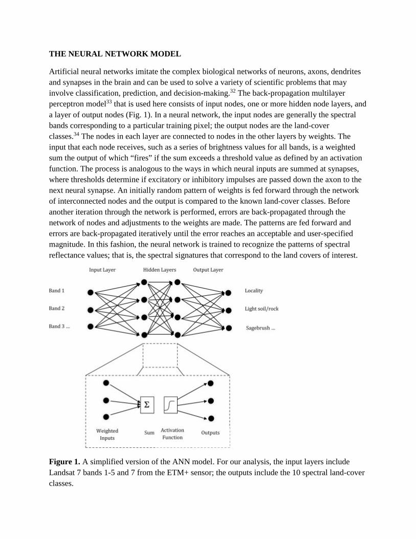
Artificial neural networks imitate the complex biological networks of neurons, axons, dendrites and synapses in the brain and can be used to solve a variety of scientific problems that may involve classification, prediction, and decision-making.32 The back-propagation multilayer perceptron model33 that is used here consists of input nodes, one or more hidden node layers, and a layer of output nodes (Fig. 1). In a neural network, the input nodes are generally the spectral bands corresponding to a particular training pixel; the output nodes are the land-cover classes.34 The nodes in each layer are connected to nodes in the other layers by weights. The input that each node receives, such as a series of brightness values for all bands, is a weighted sum the output of which “fires” if the sum exceeds a threshold value as defined by an activation function. The process is analogous to the ways in which neural inputs are summed at synapses, where thresholds determine if excitatory or inhibitory impulses are passed down the axon to the next neural synapse. An initially random pattern of weights is fed forward through the network of interconnected nodes and the output is compared to the known land-cover classes. Before another iteration through the network is performed, errors are back-propagated through the network of nodes and adjustments to the weights are made. The patterns are fed forward and errors are back-propagated iteratively until the error reaches an acceptable and user-specified magnitude. In this fashion, the neural network is trained to recognize the patterns of spectral reflectance values; that is, the spectral signatures that correspond to the land covers of interest.

Figure 1. A simplified version of the ANN model. For our analysis, the input layers include Landsat 7 bands 1-5 and 7 from the ETM+ sensor; the outputs include the 10 spectral land-cover classes.

In our model,87 the input nodes are six visible and infrared bands of electromagnetic radiation from the Landsat 7 Enhanced Thematic Mapper Plus sensor (ETM+) obtained from the USGS EROS Data Center35 based on images taken on August 8 and September 2, 2002. These dates were chosen because the images were cloud-free and were obtained before the partial failure of the ETM+ sensor in 2003. The September image was projected to the Universal Transverse Mercator Zone 12, World Geodetic System 84 coordinate system to match the August image. Each scene was calibrated using the instrument gain values, and the elevation and azimuth of the sun at the time of acquisition to yield percent reflectance images. The panchromatic bands (band 8) were used to increase the spatial resolution from the original 28.5 m to 14.25 m using a principal components approach in which the first principal component of the 28.5 m visible and reflective infrared bands (bands 1 – 5 and 7) was replaced by the high-resolution panchromatic band and back transformed to yield a pan-enhanced multispectral image. The images were then joined together to form a continuous image of the Great Divide Basin.

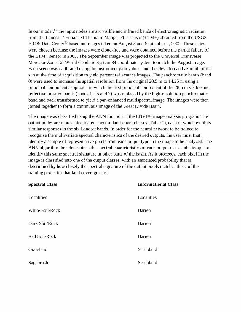
The image was classified using the ANN function in the ENVI™ image analysis program. The output nodes are represented by ten spectral land-cover classes (Table 1), each of which exhibits similar responses in the six Landsat bands. In order for the neural network to be trained to recognize the multivariate spectral characteristics of the desired outputs, the user must first identify a sample of representative pixels from each output type in the image to be analyzed. The ANN algorithm then determines the spectral characteristics of each output class and attempts to identify this same spectral signature in other parts of the basin. As it proceeds, each pixel in the image is classified into one of the output classes, with an associated probability that is determined by how closely the spectral signature of the output pixels matches those of the training pixels for that land coverage class.

Spectral Class Informational Class

Localities Localities

White Soil/Rock Barren

Dark Soil/Rock Barren

Red Soil/Rock Barren

Grassland Scrubland

Sagebrush Scrubland

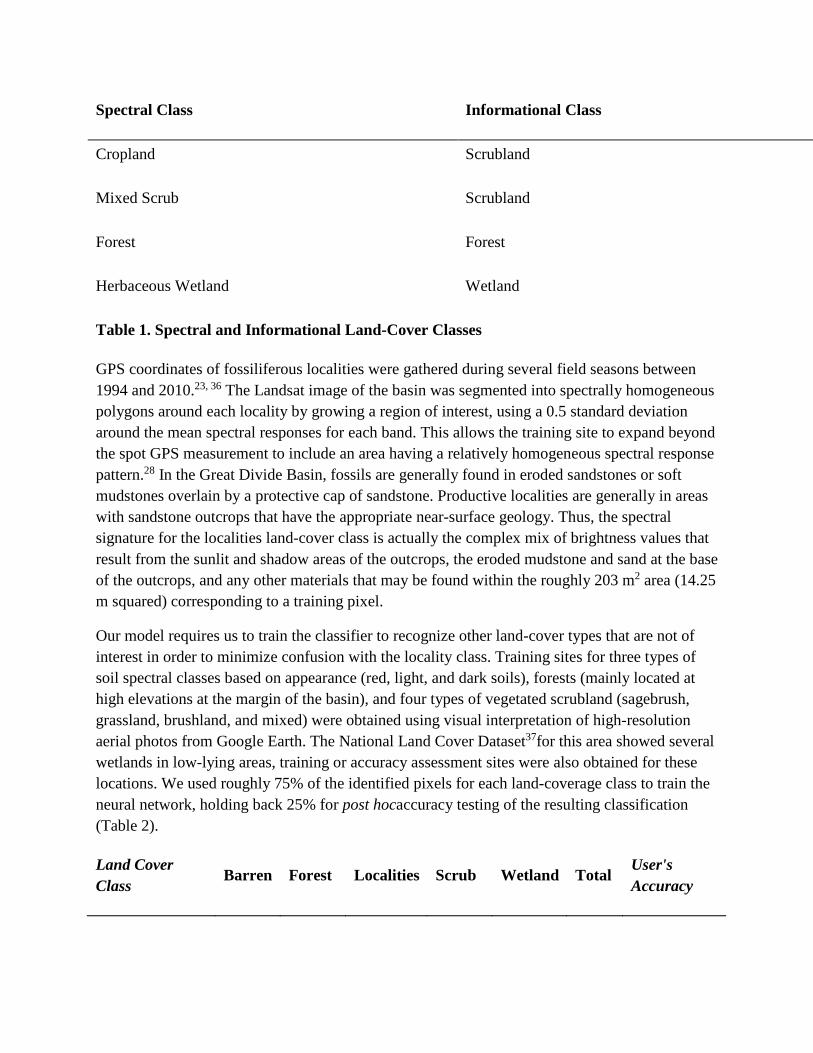
Spectral Class Informational Class

Cropland Scrubland

Mixed Scrub Scrubland

Forest Forest

Herbaceous Wetland Wetland

Table 1. Spectral and Informational Land-Cover Classes

GPS coordinates of fossiliferous localities were gathered during several field seasons between 1994 and 2010.23, 36 The Landsat image of the basin was segmented into spectrally homogeneous polygons around each locality by growing a region of interest, using a 0.5 standard deviation around the mean spectral responses for each band. This allows the training site to expand beyond the spot GPS measurement to include an area having a relatively homogeneous spectral response pattern.28 In the Great Divide Basin, fossils are generally found in eroded sandstones or soft mudstones overlain by a protective cap of sandstone. Productive localities are generally in areas with sandstone outcrops that have the appropriate near-surface geology. Thus, the spectral signature for the localities land-cover class is actually the complex mix of brightness values that result from the sunlit and shadow areas of the outcrops, the eroded mudstone and sand at the base of the outcrops, and any other materials that may be found within the roughly 203 m2 area (14.25 m squared) corresponding to a training pixel.

Our model requires us to train the classifier to recognize other land-cover types that are not of interest in order to minimize confusion with the locality class. Training sites for three types of soil spectral classes based on appearance (red, light, and dark soils), forests (mainly located at high elevations at the margin of the basin), and four types of vegetated scrubland (sagebrush, grassland, brushland, and mixed) were obtained using visual interpretation of high-resolution aerial photos from Google Earth. The National Land Cover Dataset37for this area showed several wetlands in low-lying areas, training or accuracy assessment sites were also obtained for these locations. We used roughly 75% of the identified pixels for each land-coverage class to train the neural network, holding back 25% for post hocaccuracy testing of the resulting classification (Table 2).

Land Cover Class

Barren Forest Localities Scrub Wetland Total User's Accuracy

Land Cover Class Barren Forest Localities Scrub Wetland Total User's

Accuracy

Barren 2411 19 1035 114 20 3599 66.99%

Forest 0 2402 23 193 18 2636 91.12%

Localities 35 6 5525 22 1 5589 98.85%

Scrub 12 238 408 1429 50 2137 66.87%

Wetland 0 5 0 6 11 22 50.00%

Total 2458 2670 6991 1764 100 13983

Producer's Accuracy 98.09% 89.96% 79.03% 81.01% 11.00%

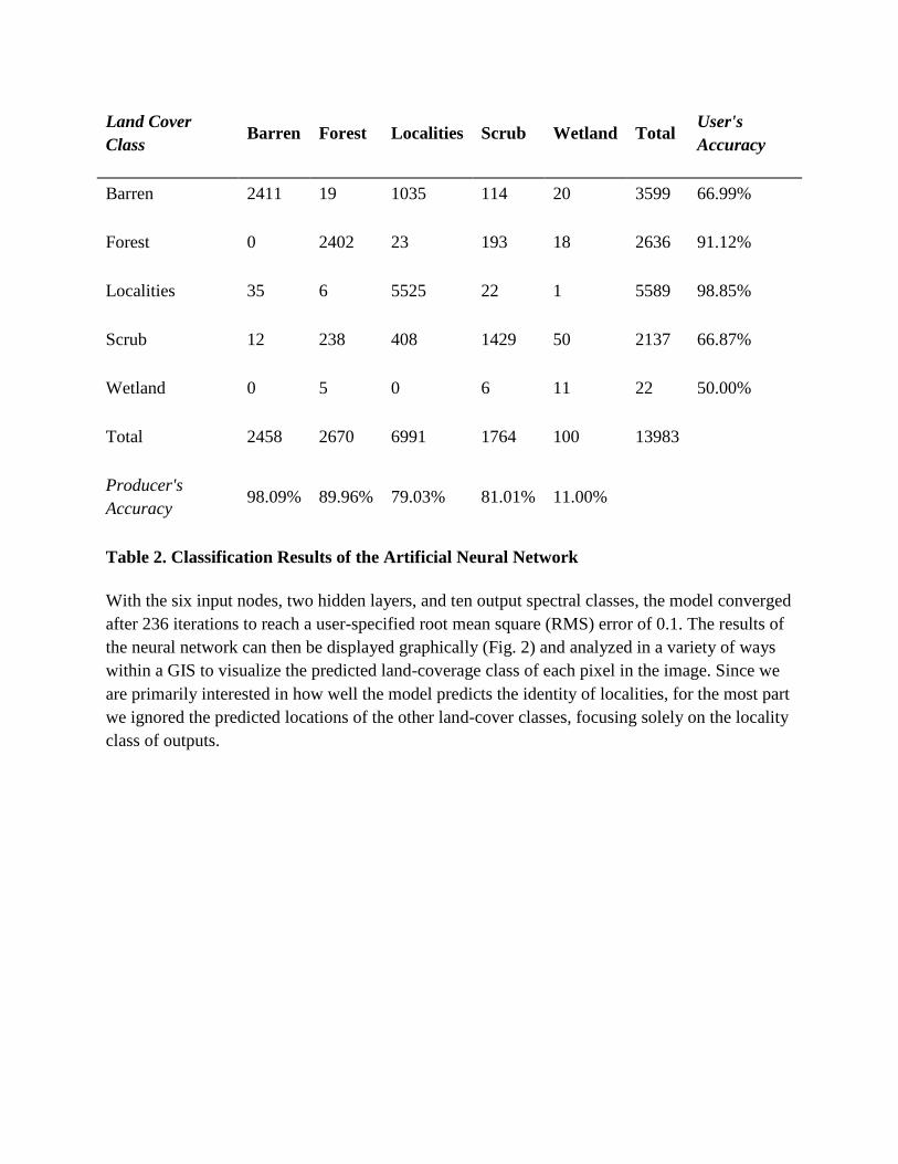
Table 2. Classification Results of the Artificial Neural Network

With the six input nodes, two hidden layers, and ten output spectral classes, the model converged after 236 iterations to reach a user-specified root mean square (RMS) error of 0.1. The results of the neural network can then be displayed graphically (Fig. 2) and analyzed in a variety of ways within a GIS to visualize the predicted land-coverage class of each pixel in the image. Since we are primarily interested in how well the model predicts the identity of localities, for the most part we ignored the predicted locations of the other land-cover classes, focusing solely on the locality class of outputs.

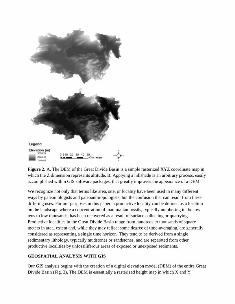
Figure 2. A. The DEM of the Great Divide Basin is a simple rasterized XYZ coordinate map in which the Z dimension represents altitude. B. Applying a hillshade is an arbitrary process, easily accomplished within GIS software packages, that greatly improves the appearance of a DEM.

We recognize not only that terms like area, site, or locality have been used in many different ways by paleontologists and paleoanthropologists, but the confusion that can result from these differing uses. For our purposes in this paper, a productive locality can be defined as a location on the landscape where a concentration of mammalian fossils, typically numbering in the low tens to low thousands, has been recovered as a result of surface collecting or quarrying. Productive localities in the Great Divide Basin range from hundreds to thousands of square meters in areal extent and, while they may reflect some degree of time-averaging, are generally considered as representing a single time horizon. They tend to be derived from a single sedimentary lithology, typically mudstones or sandstones, and are separated from other productive localities by unfossiliferous areas of exposed or unexposed sediments.

GEOSPATIAL ANALYSIS WITH GIS

Our GIS analysis begins with the creation of a digital elevation model (DEM) of the entire Great Divide Basin (Fig. 2). The DEM is essentially a rasterized height map in which X and Y

coordinates represent the geographic coordinates and Z represents elevation. We obtained the data for our DEM from the National Elevation Database (NED)38 and created it using ArcGIS software. Using ArcGIS, we resampled the NED data from an original pixel size of 10 m to 14.25 m in order to match the pixel size on our Landsat images. We also derived a hillshade layer from the DEM. This basically creates a shaded relief image with shadows resulting from an assumed sun in the northwest, thus giving the viewer an idea of the topography. This hillshade image forms the backdrop for the graphical outputs of our ANN.

IMAGE CLASSIFICATION AND RESULTS

Table 2 presents the results of post-hoc accuracy testing for the ANN's classification of the Great Divide Basin. These results measure how well the neural network model identified the 25% of known pixels in each of the five land-cover classes that were held back for this purpose during training. For accuracy assessment purposes, the three spectrally distinct bare rock or soil classes (red, light, and dark brown) were combined into a single “Barren” informational class; four different types of vegetative cover (sagebrush, grass, cropland, and mixed scrub) were combined into a single “Scrubland” informational class, yielding five informational classes of land cover for comparison (Table 1). Vertical columns in accuracy assessment results (Table 2) represent ground truth,39 meaning that the total number of pixels known to exist in each class can be found running from left to right near the bottom of the Table (for example, 2,458 pixels were known to be barren, 100 were known to be wetland, and so on). Horizontal rows represent the classified pixels for each land-cover class; the total number of pixels predicted to fall in each class can be found from top to bottom along the right side of the table (for example, 3,599 pixels were predicted to be barren and 22 were predicted to be wetland). The overall results are encouraging: the model correctly classified 84.21% of the pixels in all land-cover classes, with a Kappa coefficient (a more conservative measure of correctly classified pixels) of 77.44%. For the localities column, the model correctly classified 5,525 of the 6,991 actual locality pixels to yield a “producer's accuracy” (a measure of errors of omission in which pixels that are actually localities, for example, are incorrectly classified as something else) of 79.03%. Of the 5,589 pixels predicted to represent localities, 5,525 were known to be localities, for a “user's accuracy” (a measure of errors of commission in which pixels that were predicted to be localities actually belonged to another land-cover class) of 98.85%. Each predicted pixel comes with an associated probability, which is not represented in these tabular data. The best way to explore this is through an examination of the graphical output of the ANN, known as the classified image.

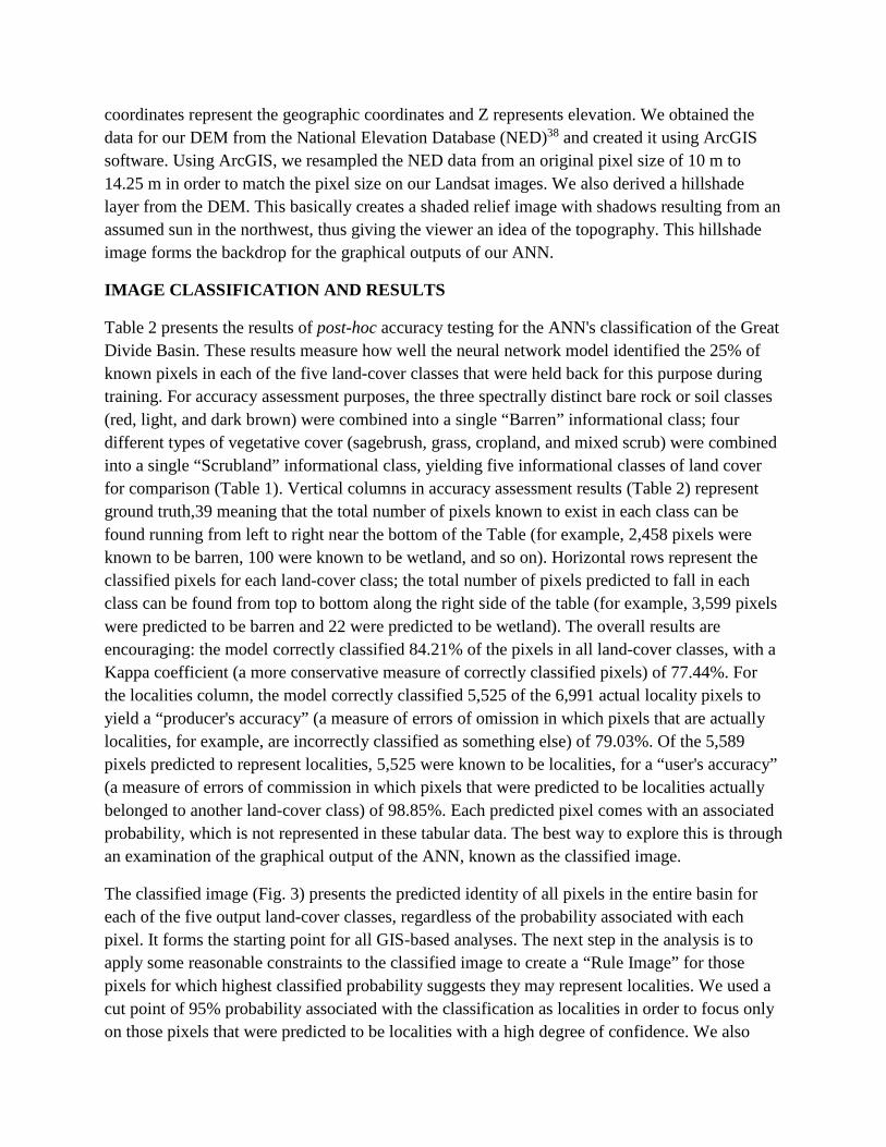
The classified image (Fig. 3) presents the predicted identity of all pixels in the entire basin for each of the five output land-cover classes, regardless of the probability associated with each pixel. It forms the starting point for all GIS-based analyses. The next step in the analysis is to apply some reasonable constraints to the classified image to create a “Rule Image” for those pixels for which highest classified probability suggests they may represent localities. We used a cut point of 95% probability associated with the classification as localities in order to focus only on those pixels that were predicted to be localities with a high degree of confidence. We also

constrained the predicted pixels to those with a slope of greater than 5% in order to ignore areas of little or no vertical relief that may spectrally resemble localities but lack active erosional surfaces where fossils tend to be found. The rule image is then displayed as a layer on top of a hillshaded DEM of the entire GDB. The results can be seen in Figure 4, where the red pixels classified as localities can be seen clustered in several parts of the GDB.

Figure 3. Classified Image. This image of the Great Divide Basin classifies each pixel into one of the five land-cover classes used in this study. All red pixels are predicted to represent localities, but their associated probability will vary from low to high.

Figure 4. Rule Image. This image of the Great Divide Basin includes in red those pixels that had a >95% of belonging to the locality class, and had a slope >5%. This represents our current best estimate of parts of the basin that may include localities with high probability and high priority for ground truthing in upcoming field seasons.

TESTING THE MODEL IN THE BISON BASIN

Directly to the north of the central part of the Great Divide Basin lies a small isolated area containing sedimentary deposits of the Fort Union Formation known as the Bison Basin (Fig. 5). The existence of fossil mammals of Tiffanian age (middle to late Paleocene) has been known there since the 1950s as a result of early work by USGS geologists and, particularly, the Smithsonian Institution paleontologist C. L. Gazin.40 During the past ten years, field crews from the Carnegie Museum of Natural History under the direction of K. C. Beard have returned to the Bison Basin to work at its three most productive localities: West End, Saddle, and Ledge. The geographic and chronological proximity of the Bison Basin vertebrate localities to those in the Great Divide Basin suggests that they might allow an interesting test of our predictive model. We view this test of our model as a conservative one since we trained our ANN to recognize fossil-bearing sediments of the Wasatch Formation of Eocene age in the Great Divide Basin. The spectral signatures of fossil-bearing units in the older Fort Union Formation might be somewhat different owing to the different lithologies and facies in that rock unit.

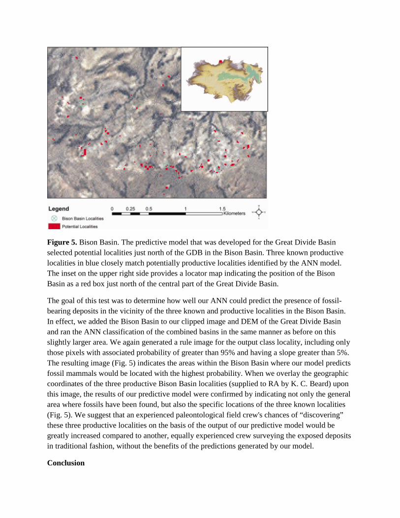
Figure 5. Bison Basin. The predictive model that was developed for the Great Divide Basin selected potential localities just north of the GDB in the Bison Basin. Three known productive localities in blue closely match potentially productive localities identified by the ANN model. The inset on the upper right side provides a locator map indicating the position of the Bison Basin as a red box just north of the central part of the Great Divide Basin.

The goal of this test was to determine how well our ANN could predict the presence of fossil-bearing deposits in the vicinity of the three known and productive localities in the Bison Basin. In effect, we added the Bison Basin to our clipped image and DEM of the Great Divide Basin and ran the ANN classification of the combined basins in the same manner as before on this slightly larger area. We again generated a rule image for the output class locality, including only those pixels with associated probability of greater than 95% and having a slope greater than 5%. The resulting image (Fig. 5) indicates the areas within the Bison Basin where our model predicts fossil mammals would be located with the highest probability. When we overlay the geographic coordinates of the three productive Bison Basin localities (supplied to RA by K. C. Beard) upon this image, the results of our predictive model were confirmed by indicating not only the general area where fossils have been found, but also the specific locations of the three known localities (Fig. 5). We suggest that an experienced paleontological field crew's chances of “discovering” these three productive localities on the basis of the output of our predictive model would be greatly increased compared to another, equally experienced crew surveying the exposed deposits in traditional fashion, without the benefits of the predictions generated by our model.

Conclusion

Our research is a first attempt to develop a predictive model to aid paleoanthropologists and vertebrate paleontologists in the critical activity of fossil exploration. We trained an artificial neural network to recognize ten different categories of land cover, including known localities, in our study area in the Great Divide Basin of Wyoming. Working with satellite images derived from the ETM+ sensor on Landsat 7, the ANN determined those areas having a high potential of being fossiliferous, due to the similarity of their spectral signatures to those of known fossil localities. The results of our model's predictions of the location of fossil-bearing localities in the nearby Bison Basin are extremely encouraging.

Box 1: The Great Divide Basin

The Great Divide Basin (GDB) of southwestern Wyoming is one of the many large structural and sedimentary basins in the Rocky Mountain region of the American West that are well known to vertebrate paleontologists.47, 48 The name comes from the fact that the Continental Divide actually splits and encircles the basin, so that when driving Interstate 80 across southern Wyoming one crosses the Continental Divide twice between Laramie and Rock Springs. The GDB contains thousands of meters of fossiliferous sedimentary rock of Cretaceous to Eocene age that are variably exposed throughout its approximately 10,000 square kilometers.49, 50 The impetus for the research reported here stems from the difficulties of determining where one's efforts might be best applied toward the goal of finding fossils in such a large geographic space.

Box 1.. The Great Divide Basin lies astride the Continental Divide in southwestern Wyoming. It is one of several large sedimentary basins in the Rocky Mountain West with extensive fossil-bearing deposits spanning the Cretaceous through the Eocene.

The first paleontologist to work in the GDB, in the 1950s and 1960s, was the Smithsonian Institution's C. L. Gazin. A series of Gazin's publications described a handful of latest Paleocene and earliest Eocene localities scattered through the basin.51–54 The specimens and localities Gazin described were sufficient to allow him to fill in the paleontological blank space that the GDB had been before his work, but compared to the richer and more productive basins in the northern and southern Rocky Mountain regions (for example, the Bighorn and Wind River Basins in the north and the San Juan and Uinta Basins in the south), the GDB languished in obscurity for decades. Beginning in 1994, the senior author began leading annual field crews to the Great Divide Basin with the dual intentions of collecting new fossils from Gazin's localities and identifying new localities in this under-studied basin. After approximately 15 summer field seasons in the GDB, we have succeeded in both of our original goals.36 Following in Gazin's footsteps, we have collected, identified, and catalogued nearly 10,000 mammalian fossils from approximately 100 localities. We succeeded in locating several of Gazin's named localities and substantially increasing the mammalian fauna from each. In 2009 we located one of the richest Wasatchian (early Eocene) mammal localities in North America from which we recovered more than 400 mammalian jaws and approximately 5,000 isolated teeth and postcranial elements.55 The realization that we located this superb new locality purely by chance challenges us in our work to develop better approaches to predicting where productive fossil-bearing localities might be identified in the future.

Paleoanthropology has for many years been an interdisciplinary field in which the tools and techniques of the natural sciences, typically applied in collaboration with geologists, chemists and physicists, have enriched our analyses of fossil primates and hominins. We suggest that the geospatial sciences have earned a place in the paleoanthropological tool kit, and that twenty-first century research in paleoanthropology must increasingly rely on the kinds of sophisticated spatial analyses that can only come from collaborations with our colleagues in the geographical and geospatial sciences. We envision a paleoanthropology that is critically engaged in the spatial analysis of the raw materials of our science at a number of hierarchical levels, ranging from the scatter of bones and artifacts at individual sites to the distribution of fossil sites within landscapes, between sedimentary basins, and across continents. While we recognize that the use of hand-held GPS receivers has become ubiquitous among field workers in many branches of biological anthropology, we encourage our colleagues to move beyond static and descriptive uses of GPS and GIS that simply record the geographic coordinates of localities or specimens. Spatial data need to be incorporated into dynamic models in order to answer a variety of important questions of paleoanthropological interest.41, 42 Some obvious candidates include migration and colonization scenarios for past human populations,43 effects of climate change on

present and past distributions of primate taxa and communities,44 and problems of dispersals, origins, and extinctions of fossil primates and other mammals.45, 46

Box 2: The Landsat Program

As a joint effort of the National Aeronautics and Space Administration (NASA) and the United States Geological Survey (USGS), the Landsat Program56 has acquired space-based images of the earth's surface continuously since the launch of Landsat 1 on July 23, 1972. In so doing, it has created a longitudinal record of natural as well as human-induced changes across the global landscape. It also provides a valuable resource to scientists working in many different fields, including agriculture and forestry, geology and geography, global climate change, and anthropology.

Of the seven Landsat missions to date, four have been decommissioned (Landsat 1-4), one failed at launch (Landsat 6), and two are still operational in 2011 (Landsat 5 and 7). Landsat 5 is still collecting imagery 27 years after its launch in 1984, well in excess of its originally planned three-year mission. Advances in scanning technology have led to significant improvements in spatial resolution and spectral bandwidth across the generations of Landsat satellites. For example, the Multispectral Scanner (MSS) carried aboard Landsat 1-3 achieved a spatial resolution of 80 m in four spectral bands ranging from visible green to near infrared wavelengths. The Thematic Mapper (TM) sensor on Landsat 4 and 5 achieved a spatial resolution of 30 m in 7 spectral bands. Landsat 7 carries the Enhanced Thematic Mapper Plus (ETM+) sensor that collects multispectral images in 8 bands spanning the visible to thermal infrared wavelengths in 185 km wide scenes with a spatial resolution of 28.5 m. Launched on April 15, 1999 and placed in orbit at an altitude of 705 km, Landsat 7 completes approximately 14 orbits each day to acquire complete coverage of the Earth's surface every 16 days. The scan line correction device in the ETM+ sensor failed in 2003, thus limiting the utility of more recent Landsat 7 imagery.

Perhaps the most remarkable feature of the remotely sensed imagery provided by the Landsat program is that the entire archive of images is now available over the Internet (http://glovis.usgs.gov/) at no charge and with no restrictions to users. The consistency and completeness of the Landsat archive make it an invaluable resource for scientists interested in detailing long-term changes to the earth's surface, as well as aiding in relief efforts by documenting before and after images of areas that have experienced natural or man-made disasters. All in all, Landsat images constitute an extremely valuable and under-used resource for vertebrate paleontologists and paleoanthropologists.

Although there are other earth-imaging satellites currently in orbit, the imagery they provide is generally not free, and in some cases, is quite expensive. The Ikonos, OrbView, and Quickbird satellites are privately owned and provide imagery with spatial resolution as high as 0.4 m. Several foreign governments also operate remote sensing satellites, including France (SPOT),

India (IRS), and a joint Chinese-Brazilian program (CBERS). The Aqua and Terra satellites operated by the U.S. National Aeronautics and Space Administration contain a number of sensors, including ASTER, which is most similar to the European SPOT series of satellites, and MODIS, which has pixel sizes ranging from 250 m to 1000 m.29 The kind of analyses described here could also be performed using imagery from any of these other sources.

Box 3. Other Uses of GIS and RS in Biological Anthropology

Biological anthropologists have used innovative new methods and techniques derived from the geographic sciences to study primates in their natural habitats, the relationship between diet and dental morphology and microwear, and the migrations out of Africa of Plio-Pleistocene hominins.4 Green and Sussman57demonstrated how satellite imagery could reveal a multi-decadal record of deforestation in the eastern forested zone of Madagascar and highlighted the conservation implications of this trend for the future of the island's mostly endemic fauna and flora. Smith, Horning, and Moore58 created a large GIS database to study habitat degradation and deforestation in western Madagascar, and evaluate how well the system of nature reserves was succeeding in safeguarding the local habitat and fauna. Recently, Irwin, Johnson, and Wright59used Landsat imagery and field censuses of 10 lemur populations to develop a multi-faceted geospatial analysis of the current ranges, available habitats, and threats to the continued existence of Madagascar's lemuriform fauna, mostly as a result of human activity. As a part of studies of global and environmental change, the analysis of RS images within GIS databases will continue to play a leading role in documenting habitat degradation and its effects on fauna and flora in many parts of the world.

The development of miniaturized GPS-enabled collars and their use in studies of animal movement and ranging behavior (that is, wildlife telemetry) has led to a revolution in the ecological study of animal behavior.60–62 Dozens of different terrestrial and marine organisms have been successfully tracked and studied by ecologists and animal behaviorists, including sea turtles,63 African elephants,64 and penguins.65A pilot study66 demonstrated the feasibility of studying baboon ranging patterns with an automated, GPS-enabled collar in the open, savannah habitats of Amboseli, Kenya. The use of such devices, and even hand-held GPS receivers, to track primates in closed canopy forest has not yet proven to be entirely feasible due to the

difficulty of obtaining the required GPS satellite signals when the sky is obscured by dense foliage.67–69

Following Denne Reed's70 initial use of three-dimensional (3-D) imaging and GIS software to study tooth morphology in 1997, several workers have applied the tools of GIS to the analysis of tooth morphology and dental microwear with the goal of understanding dietary differences among a wide variety of living and fossil primates.4 Using different approaches to collect either landmark data70 or three-dimensional point clouds derived from 3-D scanners,71, 72 a DEM of the tooth occlusal surface can be generated and analyzed using GIS software. Peter Ungar of the University of Arkansas, along with a long list of collaborators, students, and post-docs, has applied the tools of geospatial analysis to the functional morphology of teeth and patterns of dental microwear.73, 74 These approaches have been widely used in assessing microwear on extant primates of known diet, and in using the patterns that emerge to reconstruct the diet of extinct primates, including hominins. One notable success of this approach was the solution of the “worn tooth conundrum,” allowing, for the first time, the study of how wear-related changes to tooth occlusal surfaces influence dental function over an individual's lifetime.75 Ungar's innovative work constitutes a major improvement on the older techniques of counting scratches and pits on scanning electron micrographs to determine whether an animal has been fed primarily on hard or soft objects. His team has recently developed a promising new approach that uses the confocal microscope to generate a 3-D model of tooth occlusal surfaces that is then analyzed by a scale-sensitive fractal analysis76–79 to quantitatively characterize and compare patterns of microwear. Since this technique does not rely on landmark data, it can be applied to teeth at any wear stage, and since it does not involve subjective identification of scratches and pits, it should provide reproducible results with low error rates.76, 78

Two other early adopters and innovators in the application of approaches derived from the geographic and imaging sciences to the analysis of dental morphology, diet,and wear are the University of Helsinki's Jukka Jernvall and Monash University's Alistair Evans.80, 81 Working independently and together, these scholars and their colleagues have advanced the science in various ways, including use of the laser confocal microscope to generate DEMs of dental surfaces71 and the development of homology-free comparisons of dental morphology that allow quantification of the complexity of occlusal morphology (that is, orientation patch complexity, or OPC).82 A particularly interesting study scanned fossil horse teeth to study the transition to hypsodonty and grazing with increasing aridity in the European Miocene.83 Three-dimensional scans of tooth occlusal surfaces were used to create DEMs; these were analyzed with GIS software to measure the slope of the enamel surfaces, which could be related to degree of hypsodonty. In this way, the authors were able to relate evolutionary changes in dental morphology (hypsodonty) to global climate change (cooling and aridity) and diet (grazing).

Recently, Doug Boyer has been applying innovative approaches to analysis of the 3-D shape of the teeth of living and fossil primates and other mammals, the goal being to improve our ability to determine dietary preferences of fossil mammals. Building on the earlier work of Ungar,

Jernvall, and others, Boyer84 has compared extant archontans with respect to the relief index of molar shape (a ratio of tooth crown 3-D area to 2-D area that expresses the degree of hypsodonty and tooth shape complexity).74 The results suggested that variability in relief index is better correlated with diet than with phylogeny, and that it can distinguish among primate insectivores, folivores, and frugivore/gumnivores.84 More recently, Boyer has scanned the molar surfaces of three species of Plesiadapis to reveal interesting differences in both molar relief and complexity that may relate to intraspecific dietary differences.85 Boyer and colleagues86 have used a promising new measure of dental surface complexity known as Dirichlet normal energy (DNE) in the analysis of 3-D occlusal shape and diet in extant primates.86

Acknowledgements

We thank John Fleagle for the opportunity to contribute this paper and for his editorial suggestions, as well as the comments of the reviewers, all of whom greatly helped to improve the final version of this paper. Our field work in the Great Divide Basin is under federal permit 287-WY-PA95 (to RA) and administered by the Wyoming Bureau of Land Management. The permanent repository for our fossil collections is the Carnegie Museum of Natural History in Pittsburgh, PA. Bison Basin field work by Chris Beard is also permitted by the Wyoming Bureau of Land Management under federal permit 042-WY-PA98. RA thanks Mr. Walt Worthy, the Office of the Vice President for Research, and the FRACAA fund at Western Michigan University for financial support. CE acknowledges the financial support of the Lucia Harrison Endowment at Western Michigan University. We also thank our colleagues Justin Adams, Aaron Addison, Chris Beard, Wendy Dirks, Brett Nachman, Richard Stucky, and John Van Regenmorter.

REFERENCES

1. Johanson D,Taieb M. 1976. Plio-Pleistocene hominid discoveries in Hadar, Ethiopia. Nature 260: 293–297.

2. Berger LR,de Ruiter DJ,Churchill SE,Schmid P,Carlson KJ,Dirks PHGM,Kibii JM. 2010. Australopithecus sediba: a new species ofHomo-like Australopith from South Africa. Science 328: 195–204.

3. Dirks PHGM,Kibii JM,Kuhn BF,Steininger C,Churchill SE,Kramers JD,Pickering R, {JF: all aus needed.] Farber DL,Meriaux AS,Herries AIR and others. 2010. Geological setting and sge of Australopithecus sediba from Southern Africa. Science 328:205–208.

4. Anemone R,Conroy G,Emerson C. n.d. GIS and paleoanthropology: incorporating new approaches from the geospatial sciences in the analysis of primate and human evolution. Yearbk Phys Anthropol. In press.

5. Kvamme K. 1999. Recent directions and developments in geographic information systems. J Archaeol Res 7: 153–201.

6. McCoy M,Ladefoged T. 2009. New developments in the use of spatial technology in archaeology. J Archaeol Res 17: 263–295.

7. Sever T,Wiseman J. 1985. Conference on remote sensing: potential for the future. NASA Earth Resources Laboratory, NSTL, MS.

8. Johnson J,Madry S,Sever T. 1988. Remote sensing and GIS analysis in large scale survey design in north Mississippi.Southeastern Archaeology 7: 124–131.

9. Chase A,Chase D,Weishampel J,Drake J,Shrestha R,Slatton K,Awe J,Carter W. 2011. Airborne LiDAR, archaeology, and the ancient Maya landscape at Caracol, Belize. J Archaeol Sci 38: 387–398.

10. Nigro J,Limp W,Kvamme K,de Ruiter D,Berger L. 2002. The creation and potential applications of a 3-dimensional GIS for the early hominin site of Swartkrans, South Africa. In: Burenhult G,Arvidsson J, editors. Archaeological informatics: pushing the envelope CAA2001. Proceedings of the 29th Conference, Gotland, April 2001 ed. Oxford: Archaeopress. p 113–124.

11. Nigro J,Ungar P,de Ruiter D,LR B. 2003. Developing a geographic information system (GIS) for mapping and analysing fossil deposits at Swartkrans, Gauteng Province, South Africa. J Archaeol Sci 30: 317–324.

12. Mehrer M,Westcott K, editors. 2006. GIS and archaeological site location modeling. Boca Raton, FL: CRC Press.

13. Oheim KB. 2007. Fossil site prediction using geographic information systems (GIS) and suitability analysis: The Two Medicine Formation, MT, a test case. Palaeogeogr, Palaeoclimatol, Palaeoecol 251: 354–365.

14. Jennings DS,Hasiotis ST. 2006. Taphonomic analysis of a dinosaur feeding site using geographic information systems (GIS), Morrison formation, southern Bighorn Basin, Wyoming, USA. Palaios 21: 480–492.

15. Chew A,Oheim K. 2009. Using GIS to determine the effects of two common taphonomic biases on vertebrate fossil assemblages.Palaios 24: 367–376.

16. Asfaw B,Ebinger C,Harding D,White T,WoldeGabriel G. 1990. Space-based imagery in paleoanthropological research: an Ethiopian example. Natl Geo Res 6: 418–434.

17. Asfaw B,Beyene Y,Semaw S,Suwa G,White T,WoldeGabriel G. 1991. Fejej: a new paleoanthropological research area in Ethiopia.J Hum Evol 21: 137–143.

18. Fleagle JG,Rasmussen DT,Yirga S,Bown TM,Grine FE. 1991. New hominid fossils from Fejej, Southern Ethiopia. J Hum Evol 21:145–152.

19. WoldeGabriel G,White T,Suwa G,Semaw S,Beyene Y,Asfaw B,Walter R. 1992. Kesem-Kebena: a newly discovered Paleoanthropological research area in Ethiopia. J Field Archaeol 19: 471–493.

20. Wood B. 1992. A remote sense for fossils. Nature 355: 397–398. 21. Njau J,Hlusko L. 2010. Fine-tuning paleoanthropological reconnaissance with high

resolution satellite imagery: the discovery of 28 new sites in Tanzania. J Hum Evol 59: 680–684.

22. Conroy G. 2006. Creating, displaying, and querying interactive paleoanthropological maps using GIS: an example from the Uinta Basin, Utah. Evol Anthropol 15: 217–223.

23. Conroy G,Anemone R,Van Regenmorter J,Addison A. 2008. Google Earth, GIS, and the Great Divide: A new and simple method for sharing paleontological data. J Hum Evol 55: 751–755.

24. Bown T,Krause M. 1993. Soils, time, and primate paleoenvironments. Evol Anthropol 2: 11–21.

25. Shipman P. 1981. Life history of a fossil: an introduction to taphonomy and paleoecology. Cambridge, MA: Harvard University Press.

26. Asfaw B,Beyene Y,Suwa G,Walter R,White T,WoldeGabriel G,Yemane T. 1992. The earliest Acheulean from Konso-Gardula.Nature 360: 732–735.

27. Lillesand TM,Kiefer RW,Chipman JW. 2004. Remote sensing and image interpretation. New York: John Wiley and Sons.

28. Schowengerdt RA. 2007. Remote sensing models and methods for image processing. London: Elsevier.

29. Jensen JR. 2007. Remote sensing of the environment: an earth resource perspective. Upper Saddle River, NJ: Prentice-Hall.

30. Jensen JR. 2005. Introductory digital image processing: a remote sensing perspective. Upper Saddle River, NJ: Prentice-Hall.

31. Tso B,Mather TB. 2009. Classification methods for remotely sensed data. Boca Raton, FL: CRC Press.

32. Rosenblatt F. 1958. The perceptron: a probabilistic model for information storage and organization in the brain. Psychol Rev 65:386–408.

33. Rumelhart D,Hinton G,Williams RD. 1986. Learning internal representation by error propagation. In: Rumelhart D,McClelland L, editors. Distributed processing: explorations in the microstructure of cognition, Vol. 1: Foundations. Cambridge, MA: MIT Press.

34. Murai H,Omatu S. 1997. Remote sensing image analysis using a neural network and knowledge-based processing. Int J Remote Sens 18: 811–828.

35. USGS. 2011. Landsat 7 scenes L71035031_03120020808 and L71036031_03120020808. U.S. Geological Survey Earth Resources Observation and Science (EROS) Data Center accessed 05 May 2011:Available online at: edc,usgs.gov.

36. Anemone R,Dirks W. 2009. An anachronistic mammal fauna from the Paleocene Fort Union Formation (Great Divide Basin, Wyoming, USA). Geol Acta 7: 113–124.

37. Homer C,Huang C,Yang L,Wylie B,Coan M. 2004. Development of 2001 national landcover database for the United States.Photogrammetric Engineering Remote Sensing 70: 829–840.

38. Gesch D,Evans G,Mauck J,Huchinson J,Carswell W. 2009. The national map-elevation. U.S. Geological Survey Fact Sheet 3053.

39. Congalton R,Green K. 2009. Assessing the accuracy of remotely sensed data: principles and practices. Boca Raton, FL: CRC Press.

40. Gazin C. 1956. Paleocene mammalian faunas of the Bison basin in south-central Wyoming. Smithsonian Miscellaneous Collections 131: 1–57.

41. Bailey GN,Reynolds SC,King GCP. 2011. Landscapes of human evolution: models and methods of tectonic geomorphology and the reconstruction of hominin landscapes. J Hum Evol 60: 257–280.

42. Reynolds SC,Bailey GN,King GCP. 2011. Landscapes and their relation to hominin habitats: case studies from Australopithecus sites in eastern and southern Africa. J Hum Evol 60: 281–298.

43. Holmes K., 2007. GIS simulation of the earliest hominid colonisation of Eurasia. Oxford: Archaeopress.

44. Gingerich PD. 2006. Environment and evolution through the Paleocene-Eocene thermal maximum. TREE 21: 246–253.

45. Beard K,Dawson M, editors. 1998. Dawn of the age of mammals in Asia. Pittsburgh, PA: Carnegie Museum of Natural History.

46. Beard KC,Dawson MR. 1999. Intercontinental dispersal of Holarctic land mammals near the Paleocene/Eocene boundary: paleogeographic, paleoclimatic and biostratigraphic implications. Bull Soc Geol France 170: 697–706.

47. Barrs D,Bartleson B,Chapin C,Curtis B,De Voto R,Everett J,Johnson R,Mlenaar C,Peterson F,Schenk C and others. 1988. Basins of the Rocky Mountain region. In: Sloss L, editor. The geology of North America: sedimentary cover: North American Craton.Boulder, CO: Geological Society of America. p 109–220.

48. Dickinson W,Klute M,Hayes M,Janecke S,Lundin E,McKittrick M,Olivares M. 1988. Paleogeographic and paleotectonic setting of Laramide sedimentary basins in the central Rocky Mountain region. Geol Soc Am Bull 100: 1023–1039.

49. Lillegraven J. 1993. Correlation of Paleogene strata across Wyoming: a users' guide. In: Snoke A,Steidtmann J,Roberts S, editors.Geology of Wyoming: Geological Survey of Wyoming memoir No. 5.p 414–477.

50. Love JD. 1961. Definition of Green River, Great Divide, and Washakie Basins, southwestern Wyoming. Bull Am Assoc Petroleum Geol 45: 1749–1755.

51. Gazin C. 1952. The lower Eocene Knight formation of western Wyoming and its mammalian faunas. Smithsonian Miscellaneous Collections 117: 1–82.

52. [JF: Publishers' location needed.] Gazin C. 1959. Paleontological exploration and dating of the early Tertiary deposits in basins adjacent to the Uinta mountains. In: Williams N, editor. Guidebook to the geology of the Wasatch and Uinta Mountains. Intermountain Association of Petroleum Geologists. p 131–138.

53. Gazin C. 1962. A further study of the lower Eocene mammalian faunas of southwestern Wyoming. Smithsonian Miscellaneous Collections 144: 1–98.

54. Gazin C. 1965. Early Eocene mammalian faunas and their environment in the vicinity of the Rock Springs Uplift, Wyoming. Nineteenth Field Conference: Sedimentation of Late Cretaceous and Tertiary Outcrops, Rock Springs Uplift. p 171–180.

55. Anemone R,Watkins R,Nachman B,Dirks W. 2010. An early Wasatchian mammalian fauna from an extraordinarily rich new locality in the Great Divide Basin, SW Wyoming. J Vert Paleo 30( Suppl): 138A.

56. Headley R. 2010. Landsat: A global land-imaging project. Washington, DC: US Department of the Interior.

57. Green G,Sussman R. 1990. Deforestation history of the eastern rain forests of Madagascar from satellite images. Science 248:212–215.

58. Smith A,Horning N,Moore D. 1997. Regional biodiversity planning and lemur conservation with GIS in western Madagascar.Conservation Biol 11: 498–512.

59. Irwin M,Johnson S,Wright P. 2005. The state of lemur conservation in south-eastern Madagascar: population and habitat assessments for diurnal and cathemeral lemurs using surveys, satellite imagery and GIS. Oryx 39: 204–218.

60. Aarts G,MacKenzie M,McConnell B,Fedak M,Matthiopoulos J. 2008. Estimating space-use and habitat preference from wildlife telemetry data. Ecography 31: 140–160.

61. Hulbert I,French J. 2001. The accuracy of GPS for wildlife telemetry and habitat mapping. J Appl Ecol 38: 869–878.

62. Cagnacci F,Boitani L,Powell R,Boyce M. 2010. Animal ecology meets GPS-based radiotelemetry: a perfect storm of opportunities and challenges. Philos Trans R Soc B 365: 2157–2162.

63. Schofield G,Bishop CM,MacLean G,Brown P,Baker M,Katselidis KA,Dimopoulos P,Pantis JD,Hays GC. 2007. Novel GPS tracking of sea turtles as a tool for conservation management. J Exp Marine Biol Ecol 347: 58–68.

64. Blake S,Douglas-Hamilton I,Karesh W. 2001. GPS telemetry of forest elephants in Central Africa: results of a preliminary study. Afr J Ecol 39: 178–186.

65. Ryan PG,Petersen SL,Peters G,Grémillet D. 2004. GPS tracking a marine predator: the effects of precision, resolution and sampling rate on foraging tracks of African Penguins. Marine Biol 145: 215–223.

66. Markham A,Altmann J. 2008. Remote monitoring of primates using automated GPS technology in open habitats. Am J Primatol70: 1–5.

67. Dominy NJ,Duncan B. 2001. GPS and GIS methods in an African rain forest: applications for tropical ecology and conservation.Conservation Ecol 5:6.

68. Phillips K,Elvey C,Abercrombie C. 1998. Applying GPS to the study of primate ecology: a useful tool? Am J Primatol 46: 167–172.

69. [JF: Title of article strange. Is it correct?] Sprague D,Kabaya H,Hagihara K. 2004. Field testing a global positioning system (GPS) collar on a Japanese monkey: reliability of automatic GPS positioning in a Japanese forest. Primates 45: 151–154.

70. Reed D. 1997. Contour mapping as a new method for interpreting diet from tooth morphology. Am J Phys Anthropol (suppl) 24:194.

71. Jernvall J,Selanne L. 1999. Laser confocal microscopy and geographic information systems in the study of dental morphology.Palaeontol Electronica 2: 18.

72. Zuccotti L,Williamson M,Limp W,Ungar P. 1998. Modeling primate occlusal topography using geographic information systems technology. Am J Phys Anthropol 107: 137–142.

73. Ungar P. 2004. Dental topography and diets of Australopithecus afarensis and early Homo. J Hum Evol 46: 605–622.

74. Ungar P,Williamson M. 2000. Exploring the effects of tooth wear on functional morphology: a preliminary study using dental topographic analysis. Palaeontol Electronica 3: 18pp.

75. Ungar P,Simon J,Cooper J. 1991. A semiautomated image analysis procedure for the quantification of dental microwear.Scanning 13: 31–36.

76. Scott J,Godfrey L,Jungers W,Scott R,Simons E,Teaford M,Ungar P,Walker A. 2009. Dental microwear texture analysis of two families of subfossil lemurs from Madagascar. J Hum Evol 56: 405–416.

77. Scott R,Ungar P,Bergstrom T,Brown C,Childs B,Teaford M,Walker A. 2006. Dental microwear texture analysis: technical considerations. J Hum Evol 51: 339–349.

78. Scott R,Ungar P,Bergstrom T,Brown C,Grine F,Teaford M,Walker A. 2005. Dental microwear texture analysis shows within-species diet variability in fossil hominins. Nature 436: 693–695.

79. Ungar P,Brown C,Bergstrom T,Walker A. 2003. Quantification of dental microwear by tandem scanning confocal microscopy and scale-sensitive fractal analysis. Scanning 25: 185–193.

80. Evans A. 2005. Connecting morphology, function and tooth wear in microchiropterans. Biol J Linn Soc 85: 81–96.

81. Evans A,Sanson G. 2003. The tooth of perfection: functional and spatial constraints on mammalian tooth shape. Biol J Linnaeus Soc 78: 173–191.

82. Evans A,Wilson G,Fortelius M,Jernvall J. 2007. High level similarity of dentitions in carnivorans and rodents. Nature 445: 78–81.

83. Eronen J,Evans A,Fortelius M,Jernvall J. 2009. The impact of regional climate on the evolution of mammals: a case study using fossil horses. Evolution 64: 398–408.

84. Boyer D. 2008. Relief index of second mandibular molars is a correlate of diet among prosimian primates and other euarchontan mammals. J Hum Evol 55: 1118–1137.

85. Boyer D,Evans A,Jernvall J. 2010. Evidence of dietary differentiation among late Paleocene-early Eocene plesiadapids (Mammalia, Primates). Am J Phys Anthropol 142: 194–210.

86. Bunn J,Boyer D,Lipman Y,St. Clair E,Jernvall J,Daubechies I. 2011. Comparing Dirichlet normal surface energy of tooth crowns, a new technique of molar shape quantification for dietary inference, with previous methods in isolation and in combination. Am J Phys Anthropol 145: 247–261.

87. Emerson C,Anemone R. 2012. An artificial neural network-based approach to identifying mammalian fossil localities in the Great Divide Basin, Wyoming. Remote Sensing Letters 460: 453–460.