
feb-fresenius environmental bulletin
305
-
Upload
khangminh22 -
Category
Documents
-
view
1 -
download
0
Transcript of feb-fresenius environmental bulletin


FEB-FRESENIUS ENVIRONMENTAL BULLETIN
Founded jointly by F.Korte and F.Coulston
Production by PSP-Vimy str 1e,85354 Freising,Germany in
cooperation with PRT-Parlar Research & Technology
Vimy Str 1e,85354 Freising
Copyright© by PSP and PRT,Vimy Str 1e,85354 Freising,Germany
All rights are reserved,especially the right to translate into foreign language or other processes-or
converted to a machine language,especially for data processing equipment-without written permission of the
publisher.The rights of reproduction by lecture,radio and television transmission,magnetic sound recording or
similar means are also reserved.
Printed in Germany-ISSN 1018-4619

by PSP Volume 25 – No. 2/ 2016 Fresenius Environmental Bulletin
FEB-EDITORIAL BOARD
Chief Editor : Managing Editor:
Prof.Dr.Dr.H.Parlar Dr.P.Parlar
Parlar Research & Technology-PRT Parlar Research&Technology
Vimy Str.1e PRT,Vimy Str.1e
85354 Freising ,Germany 85354 Freising-Germany
Co-Editors:
Environmental Spectroscopy Environmental Management Prof.Dr.A.Piccolo Prof.Dr.F.Vosniakos
Universita di Napoli”FredericoII” TEI-Thessaloniki,Applied Physic
Dipto.Di Scienze Chmica Agrarie P.O-Box 14561
Via Universita 100,80055 Portici,Italy Thessaloniki-Greece
Environmental Biology Dr.K.I.Nikolaou
Prof.Dr.G.Schüürmann Env.Protection of Thessaloniki
UFZ-Umweltzentrum OMPEPT-54636 Thessaloniki
Sektion Chemische Ökotoxikologie Greece
Leipzig-Halle GmbH, Environmental Toxicology
Permoserstr.15,04318 Prof.Dr.H.Greim
04318 Leipzig-Germany Senatkommision-DFG/TUM
Prof.Dr.I.Holoubek 85350 Freising,Germany
Recetox-Tocoen
Kamenice126/3, 62500 Brno,Czech Republic Advisory Board
Environmental Analytical Chemistry K.Bester,K.Fischer,R.Kallenborn
Prof.Dr.M.Bahadir DCG.Muir,R.Niessner,W.Vetter,
Lehrstuhl für Ökologische Chemie A.Reichlmayr-Lais,D.Steinberg ,
und Umweltanalytik J.P.Lay,J.Burhenne,L.O.Ruzo
TU Braunschweig Marketing Manager
Lehrstuhl für Ökologische Chemie Cansu Ekici,Bc of BA
Hagenring 30, 38106 Braunschweig PRT-Research and Technology
Germany Vimy Str 1e
Dr.D.Kotzias 85354 Freising,Germany
Via Germania29 E-Mail:[email protected]
21027 Barza(Va) [email protected]
Italy Phone:+498161887988

by PSP Volume 25 – No. 2/ 2016 Fresenius Environmental Bulletin
Fresenius Environmental Bulletin is abstracted/indexed in:
Biology&Environmental Sciences,BIOSIS,CAB International,Cambridge Scientific
abstracts,Chemical Abstracts,Chemical Abstracts,Current Awareness,Current
Contents/Agriculture,CSA Civil Engineering Abstracts,CSA
Mechanical&Transportation Engineering,IBIDS database,Information
Ventures,NISC,research Alert,Science Citation Indey(SCI),Scisearch,Selected Water
Resources Abstracts
© by PSP Volume 25 – No. 2/2016, pages 370-372 Fresenius Environmental Bulletin
370
CONTENTS ORIGINAL PAPERS ENDOCRINE DISCRUPTERS IN AQUEOUS DEGRADATION OF FOUR ENVIRONMENTAL SOLUTIONS BY
OZONIZATION “MECHANISM AND INFLUENCE OF pH”
373
Yang Gang, Xiang Qiming, Zhang Beibei, Yu Dian, Chen Jiexia, Deng Chao
INDUSTRIAL EXPERIMENTAL STUDY ON SO2 REMOVAL DURING NOVEL INTEGRATED SINTERING FLUE GAS
DESULFURIZATION PROCESS
384
Qin Linbo, Han Jun, Deng Yurui, He Chao, Chen Wangsheng
THE PREPARATION OF Ag/Cu2O HOLLOW NANOSPHERES FOR ENHANCED PHOTOCATALYTIC ACTIVITY 391
Zhufeng Lu, Hongmei Wang, Dapeng Zhou, Dan Liu, Zhe Chen
DETERMINATION OF LEAD, MERCURY, ARSENIC AND CADMIUM LEVEL IN MUSCLE OF COMMON CARP
(CYPRINUS CARPIO) IN SOUTHERN CASPIAN SEA AND GOMISHAN AND ANZALI WETLANDS
401
Mohammad Reza Ghomi
RENEWABLE ENERGY STATUS AND HYDROPOWER IN SOME DEVELOPING COUNTRIES AND FOCUS ON
TURKEY
409
Ibrahim Yuksel, Hasan Arman, Ugur Serencam, Mehmet Songur, I. Halil Demirel
RESEARCH ON VEGETATION ECOLOGICAL RISK ASSESSMENT BASED ON RRM -TAKE XIANGXI RIVER
HYDRO-FLUCTUATION BELT OF THREE GORGES RESERVOIR AREA AS AN EXAMPLE
419
Haiyan Li, Peijiang Zhou, Chao Xu, Wanshun Zhang, Guoqiang Song
EFFECTS OF SOME BOTANICAL INSECTICIDES ON THE EGG PARASITOID TRICHOGRAMMA PINTOI VOEGELÉ
(HYMENOPTERA: TRICHOGRAMMATIDAE)
429
Hilal Tunca, Sahin Tatlı, H. Hilal Moran, Cem Özkan
ESTIMATING THE SOIL REDISTRIBUTION RATES IN A SMALL AGRICULTURAL REGION (KARKIN VILLAGE) IN
GEDIZ BASIN BY USING 137CS AND 210PB MEASUREMENTS
444
Manav Ramazan, Görgün Ugur Aysun, Özden Banu, Arslan Fatih Dursun
DISTRIBUTION AND BIOAVAILABILITY OF NITROGEN AND PHOSPHORUS FRACTIONS IN STREET DUSTS OF
MEGA-CITY, CHENGDU, SOUTHWEST CHINA
453
Bin Zhang, Chi Xu, Shumin Wang, Chunmei Wei
OPTIMIZED PARAMETERIZATION FOR SPATIAL INTERPOLATION OF DAILY TEMPERATURE DATA AT BLACK
SEA REGION, TURKEY
464
Emine Tanır Kayıkçı, Selma Zengin Kazancı
RISK ASSESSMENT OF HEAVY METALS IN FARMLAND SOILS NEAR MINING AREAS IN DAYE CITY, HUBEI
PROVINCE, CHINA
490
Yongkui Wang, Chunqin Yin, Jiaquan Zhang, Xianli Liu, Wei Kang, Liang Liu, Wensheng Xiao
© by PSP Volume 25 – No. 2/2016, pages 370-372 Fresenius Environmental Bulletin
371
DEGRADATION OF 2-NITROPHENOL FROM PETROCHEMICAL WASTEWATER BY
UV/NIFE2O4/CLINOPTILOLITE PROCESS
500
Aref Shokri, Kazem Mahanpoor, Davood Soodbar
MITROCHONDRIAL DNA CONTROL REGION POLYMORPHISMS OF LOGGERHEAD AND GREEN TURTLES
NESTING ON TURKISH BEACHES: QUICK RESULTS WITH RESTRICTION FRAGMENT LENGTH POLYMORPHISM
(RFLP) ANALYSIS FOR CONSERVATION ASSESSMENT
509
Arzu Kaska
EFFECTS OF LOW MOLECULAR WEIGHT ORGANIC ACIDS ON PHOSPHORUS ADSORPTION CHARACTERISTICS
IN A BLACK CLAY SOIL IN NORTHEAST CHINA
517
Yongzhuang Wang, Baoqing Hu, Yan Yan
CONTAMINATION STATUS OF ERZENI RIVER, ALBANIA DUE TO HEAVY METALS SPATIAL AND TEMPORAL
DISTRIBUTION
525
Alma Shehu, Majlinda Vasjari, Edlira Baraj, Rajmonda Lilo, Roza Allabashi
ANALYSIS ON REGIONAL CLIMATE AND ATMOSPHERIC DROUGHT CHARACTERISTICS IN THE NORTH SLOPE
OF TIANSHAN MOUNTAIN IN XINJIANG, CHINA
534
Aihong Fu, Yaning Chen, Weihong Li
THE CHARACTERISTICS OF SOIL WATER EVAPORATION IN THE CORN FIELDS UNDER DIFFERENT CLIMATE
CONDITIONS IN ARID REGIONS OF NORTHWESTERN CHINA
548
Aihong Fu, Weihong Li, Yaning Chen
SHORT AND LONG TERM STREAMFLOW PREDICTION BY DIFFERENT NEURAL NETWORK APPROACHES AND
TREND ANALYSIS METHODS: CASE STUDY OF SAKARYA RIVER, TURKEY
565
Osman Sonmez, Gokmen Ceribasi, Emrah Dogan
EFFECT OF THE IRON CONCENTRATION ON THE PROPERTIES OF AN ALUMINOSILICATE GLASS USED FOR
STORAGE OF RADIOACTIVE WASTE
580
D. Moudir, S. Ikhaddalene, N. Kamel, A. Benmounah, F. Zibouche, Y. Mouheb, F. Aouchiche
ADSORPTION OF CR(VI) ONTO BIOCHARS DERIVED FROM TYPICAL VEGETABLE OIL CROP BIOMASSES
ORIGINATING IN LOESS AREAS
588
Baowei Zhao, Xiaying Shi, Fengfeng Ma
REMEDIATION EFFECTS OF MAIZE-STRAW-DERIVED BIOCHAR ON RICE GROWN IN CADMIUM-
CONTAMINATED SOIL IN NORTH CHINA
602
Weiming Zhang, Liqun Xiu, Wenfu Chen
TOXIC EFFECTS OF SILICA NANOPARTICLES ON HEART: ELECTROPHYSIOLOGICAL, BIOCHEMICAL,
HISTOLOGICAL AND GENOTOXIC STUDY
612
Ebru Ballı, Ülkü Çömelekoğlu, Serap Yalın, Dilek Battal, Kasım Ocakoğlu, Fatma Söğüt, Selma Yaman, Çağatay Han Türkseven, Pelin Eroğlu, İlkay Karagül, Gülşen Göney, Saadet Yıldırımcan, Ayça Aktaş
INFLUENCE OF LEAD STRESS ON GROWTH, ANTIOXIDATIVE ENZYME ACTIVITIES AND ION CHANGE IN
ROOT AND LEAF OF STRAWBERRY
623
Ferhad Muradoğlu, Tarık Encu, Muttalip Gündoğdu, Sibel Boysan Canal

© by PSP Volume 25 – No. 2/2016, pages 370-372 Fresenius Environmental Bulletin
372
INFLUENCE OF ALKALI CATALYSTS ON THE SUPERCRITICAL WATER GASIFICATION OF CYANOBACTERIA 633
Huiwen Zhang, Wei Zhu, Miao Gong, Yujie Fan
RELATIONSHIPS BETWEEN SELECTED SOIL PROPERTIES EXAMINED BY THE LUCAS PROJECT AND
SATELLITE-DERIVED VEGETATION INDICES FOR POLAND
641
Dariusz Gozdowski
EFFECTS OF ORGANIC FERTILIZER INPUT ON HEAVY METAL CONTENT AND SPECIATION IN VEGETABLE
AND SOIL
647
Yaning Han, Mengmeng Rui, Yi Hao, Yukiu Rui, Xinlian Tang, Liming Liu, Weidong Cao
SHORT TERM EFFECTS OF ZINC ON SOME SERA BIOCHEMICAL PARAMETERS AND ON TISSUE
ACCUMULATION OF CLARIAS GARIEPINUS
658
Mustafa Tuncsoy, Servet Duran, Burcu Yesilbudak, Özcan Ay, Bedii Cicik, Cahit Erdem
by PSP Volume 25 – No. 2/2016, pages 373-383 Fresenius Environmental Bulletin
373
ENDOCRINE DISCRUPTERS IN AQUEOUS DEGRADATION OF FOUR ENVIRONMENTAL SOLUTIONS BY
OZONIZATION “MECHANISM AND INFLUENCE OF pH”
Yang Gang¹’²,Xiang Qiming¹*,Zhang Beibei¹,Yu Dian¹,Chen Jiexia¹,Deng Chao1
¹State Key laboratory of Pollution and Research Reuse,School of Environment,Nanjing University,Nanjing 210023,China
²College of Environment,Shichuan Agroculture University,Chendu 611130,China
ABSTRACT
This work investigated the degradation of four
environmental endocrine disrupters (EDCs)
including estrone (E1), 17β-estradiol (E2), 17α-
Ethinylestradiol (EE2) and estriol (E3) by the
ozonation process. Batch experiments were carried
out to clarify the effect of ozone dosage at different
pHs on their degradation. The formed by-products
during the ozonation were identified by LC-MS.
Results indicated that ozonation was high-efficient
for removing EDCs from aqueous solutions. The
degradation efficiency of E1 could be up to almost
100% with ozone dosage of 1.2 mg·min-1 after 3
min ozonation. pH play an important role on EDCs
degradation efficiency. The effect of pH on the
degradation of these estrogens was different. When
pH value was varied from 9.0 to 11.0, the
degradation of EDCs presented to be more efficient,
but their difference of these 4 four estrogens was
not significant. As pH was in the range of 3.0-5.0,
the degradation efficiency was relatively decreased,
but the degradation difference between these
estrogens was obvious. However, only a few
compounds of the produced by-products during the
EDCs ozonation processes could be identified and
confirmed.
KEYWORDS: EDCs; Ozonation; pH; By-products
INTRODUCTION
Estrogens include natural estrogens (estrone,
estradiol, estriol) and synthetic estrogens
(Ethinylestradiol), which are effective endocrine
disruptors chemicals (EDCs) at ng·l-1 levels and the
major substances are responsible for estrogenic
activity in environment (Routledge et al., 1998).
Most of estrogens are released into the environment
via wastewater treated effluents because they are
hydrophobic compounds and uneasily degraded,
and only partially can be removed through
conventional domestic wastewater treatment plants
(WWT) processes (Auriol et al., 2006; Zhang et al.,
2008; Zhang et al.,2012). Thus, in consideration of
the presence of EDCs in sewage treatment plants
and sources of potable water, investigations of
transformation and degradation of the estrogens in
the environment, especially in aquatic environment,
has become a remarkable issue of worldwide
concerns (Zhou et al, 2007; Rodriguez et al., 2004;
Ölmez-Hanci et al. 2012).
Up till now, the researches about estrogen’s oxidation and degradation in the environment are
fewer. As the most common pre-oxidants or
disinfectants in the drinking water treatment,
Chlorine, chloramines, chlorine dioxide and ozone
are widely employed in application (Pereira et al.,
2011). Ozone is unstable in water comparing with
the chlorine or chlorine dioxide. Furthermore, it is
also characterized by the decomposition into OH
radicals (·OH), which are the strongest oxidants in
water (von Gunten, 2003). Some studies proved
that ozonation treatment is both efficient and
economical for many pollutants with the end-
products of CO2 and H2O in special conditions (Lee
et al., 2008; Kepa et al, 2008). However, ozone do
not always achieve the complete mineralization of
the pollutants although it presents high reactivity
(Bila et al,.2007), which may potentially leads to a
wide variety of by-products (Han et
al.,2004).Therefore, it is very important to know the
formation of by-products and transformations
during oxidation.
In this study, we selected 4 estrogenic
chemicals including estrone (E1), 17-βestradiol (E2), 17α-Ethinylestradiol (EE2) and estriol (E3),
as target compounds to investigate their degradation
by ozonation. The influence of ozone dosage and
pH on the removal of these substances, and the
formation of by-products in aqueous solution were
also discussed.
MATERIAL AND METHODS
Chemicals and stock solutions. Estrone (E1),
17β-estradiol (E2), 17α-Ethinylestradiol (EE2) and
by PSP Volume 25 – No. 2/2016, pages 373-383 Fresenius Environmental Bulletin
374
estriol (E3) were supplied by the J&K Chemical
Company with the purity of 99%, 99%, 98%, and
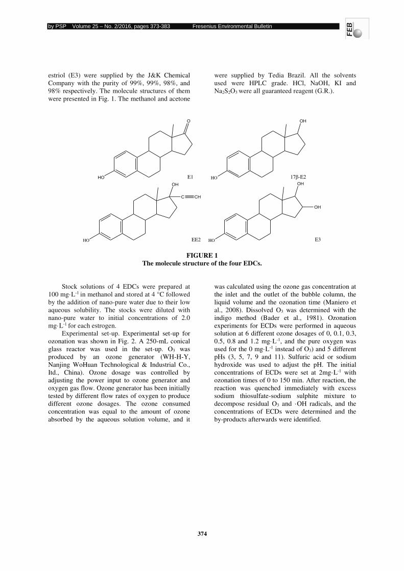
98% respectively. The molecule structures of them
were presented in Fig. 1. The methanol and acetone
were supplied by Tedia Brazil. All the solvents
used were HPLC grade. HCl, NaOH, KI and
Na2S2O3 were all guaranteed reagent (G.R.).
HO
O
E1 HO
OH
17β-E2
HO
OH
C CH
EE2 HO
OH
OH
E3
FIGURE 1 The molecule structure of the four EDCs.
Stock solutions of 4 EDCs were prepared at
100 mg·L-1 in methanol and stored at 4 °C followed
by the addition of nano-pure water due to their low
aqueous solubility. The stocks were diluted with
nano-pure water to initial concentrations of 2.0
mg·L-1 for each estrogen.
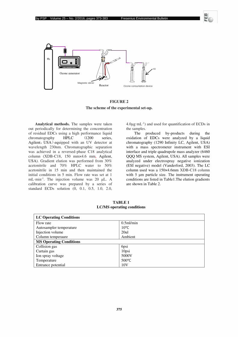
Experimental set-up. Experimental set-up for
ozonation was shown in Fig. 2. A 250-mL conical
glass reactor was used in the set-up. O3 was
produced by an ozone generator (WH-H-Y,
Nanjing WoHuan Technological & Industrial Co.,
Itd., China). Ozone dosage was controlled by
adjusting the power input to ozone generator and
oxygen gas flow. Ozone generator has been initially
tested by different flow rates of oxygen to produce
different ozone dosages. The ozone consumed
concentration was equal to the amount of ozone
absorbed by the aqueous solution volume, and it
was calculated using the ozone gas concentration at
the inlet and the outlet of the bubble column, the
liquid volume and the ozonation time (Maniero et
al., 2008). Dissolved O3 was determined with the
indigo method (Bader et al., 1981). Ozonation
experiments for ECDs were performed in aqueous
solution at 6 different ozone dosages of 0, 0.1, 0.3, 0.5, 0.8 and 1.2 mg·L-1, and the pure oxygen was
used for the 0 mg·L-1 instead of O3) and 5 different
pHs (3, 5, 7, 9 and 11). Sulfuric acid or sodium
hydroxide was used to adjust the pH. The initial
concentrations of ECDs were set at 2mg·L-1 with
ozonation times of 0 to 150 min. After reaction, the
reaction was quenched immediately with excess
sodium thiosulfate-sodium sulphite mixture to
decompose residual O3 and ·OH radicals, and the
concentrations of ECDs were determined and the
by-products afterwards were identified.
by PSP Volume 25 – No. 2/2016, pages 373-383 Fresenius Environmental Bulletin
375
FIGURE 2
The scheme of the experimental set-up.
Analytical methods. The samples were taken
out periodically for determining the concentration
of residual EDCs using a high performance liquid
chromatography HPLC 1200 series,
Agilent,USA equipped with an UV detector at
wavelength 230nm. Chromatographic separation
was achieved in a reversed-phase C18 analytical
column (XDB-C18, 150 mm×4.6 mm, Agilent,
USA). Gradient elution was performed from 30%
acetonitrile and 70% HPLC water to 50%
acetonitrile in 15 min and then maintained the
initial conditions in 5 min. Flow rate was set at 1
mL·min-1. The injection volume was 20 μL. A
calibration curve was prepared by a series of
standard ECDs solution (0, 0.1, 0.5, 1.0, 2.0,
4.0μg·mL-1) and used for quantification of ECDs in
the samples.
The produced by-products during the
oxidation of EDCs were analyzed by a liquid
chromatography (1290 Infinity LC, Agilent, USA)
with a mass spectrometer instrument with ESI
interface and triple quadrupole mass analyzer (6460
QQQ MS system, Agilent, USA). All samples were
analyzed under electrospray negative ionization
(ESI negative) model (Vanderford, 2003). The LC
column used was a 150×4.6mm XDB-C18 column
with 5 μm particle size. The instrument operating conditions are listed in Table1.The elution gradients
are shown in Table 2.
TABLE 1 LC/MS operating conditions
LC Operating Conditions
Flow rate
Autosampler temperature
Injection volume
Column temperaure
0.5ml/min
10℃20ul
Ambient
MS Operating Conditions Collision gas
Curtain gas
Ion spray voltage
Temperature
Entrance potential
6psi
10psi
5000V
500℃10V
O2
Ozone generator
Ozone consumption device Reactor
KI
Magnetic stirrer
by PSP Volume 25 – No. 2/2016, pages 373-383 Fresenius Environmental Bulletin
376
TABLE 2 The settlement of elution gradients by LC
Time Solvent A(water) Solvent B(acetonitrile)
0.00
6.00
15.00
24.00
25.00
30.00
70
70
50
50
70
70
30
30
50
50
30
30
RESULTS AND DISCUSSION
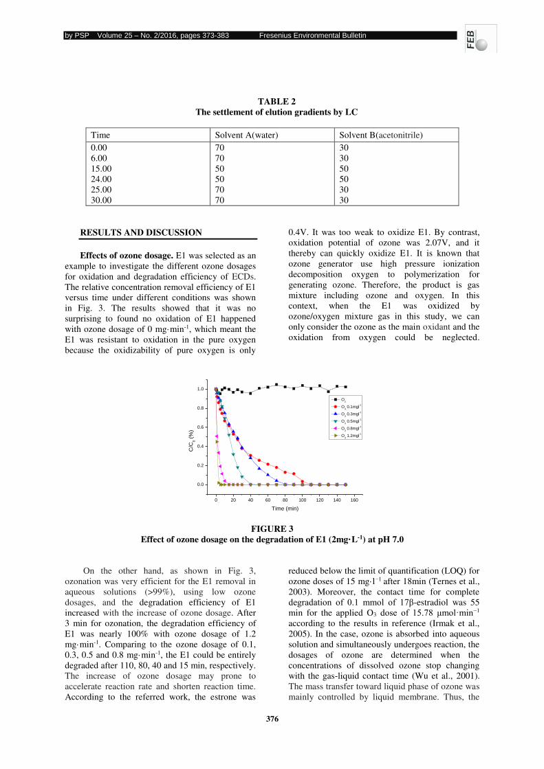
Effects of ozone dosage. E1 was selected as an
example to investigate the different ozone dosages
for oxidation and degradation efficiency of ECDs.
The relative concentration removal efficiency of E1
versus time under different conditions was shown
in Fig. 3. The results showed that it was no
surprising to found no oxidation of E1 happened
with ozone dosage of 0 mg·min-1, which meant the
E1 was resistant to oxidation in the pure oxygen
because the oxidizability of pure oxygen is only
0.4V. It was too weak to oxidize E1. By contrast,
oxidation potential of ozone was 2.07V, and it
thereby can quickly oxidize E1. It is known that
ozone generator use high pressure ionization
decomposition oxygen to polymerization for
generating ozone. Therefore, the product is gas
mixture including ozone and oxygen. In this
context, when the E1 was oxidized by
ozone/oxygen mixture gas in this study, we can
only consider the ozone as the main oxidant and the
oxidation from oxygen could be neglected.
FIGURE 3 Effect of ozone dosage on the degradation of E1 (2mg·L-1) at pH 7.0
On the other hand, as shown in Fig. 3,
ozonation was very efficient for the E1 removal in
aqueous solutions (>99%), using low ozone
dosages, and the degradation efficiency of E1
increased with the increase of ozone dosage. After
3 min for ozonation, the degradation efficiency of
E1 was nearly 100% with ozone dosage of 1.2
mg·min-1. Comparing to the ozone dosage of 0.1,
0.3, 0.5 and 0.8 mg·min-1, the E1 could be entirely
degraded after 110, 80, 40 and 15 min, respectively.
The increase of ozone dosage may prone to
accelerate reaction rate and shorten reaction time.
According to the referred work, the estrone was
reduced below the limit of quantification (LOQ) for
ozone doses of 15 mg·l−1 after 18min (Ternes et al.,
2003). Moreover, the contact time for complete
degradation of 0.1 mmol of 17β-estradiol was 55
min for the applied O3 dose of 15.78 μmol·min−1
according to the results in reference (Irmak et al.,
2005). In the case, ozone is absorbed into aqueous
solution and simultaneously undergoes reaction, the
dosages of ozone are determined when the
concentrations of dissolved ozone stop changing
with the gas-liquid contact time (Wu et al., 2001).
The mass transfer toward liquid phase of ozone was
mainly controlled by liquid membrane. Thus, the
0 20 40 60 80 100 120 140 160
0.0
0.2
0.4
0.6
0.8
1.0
C/C
0 (
%)
Time (min)
O2
O3 0.1mgl
-1
O3 0.3mgl
-1
O3 0.5mgl
-1
O3 0.8mgl
-1
O3 1.2mgl
-1
by PSP Volume 25 – No. 2/2016, pages 373-383 Fresenius Environmental Bulletin
377
mass transfer coefficient of liquid phase could be
increased when ozone dosage was increased.
Correspondingly, the amount of input ozone in a
certain time duration and solution volume was also
increased, which had a positive influence on
ozonation process (Lin et al., 2009).
Effects of pH. Ozone is unstable in water, and
the major secondary oxidant derived from ozone
decomposition in water is hydroxyl radical (HO·)
(von Gunten, 2003). In the ozonation reaction,
pollutants are oxidized by the ozone molecule or by
the HO· which derived from ozone decomposition
(Nakada et al., 2007).The stability of ozone largely
depends on the water matrix, especially the pH, the
content and type of natural organic matters (NOM)
and their alkalinity (Hoigné,1998). It is well known
that hydroxide ions initiate ozone decomposition,
which involves the 6 reactions as presented in Eq.1-
6 (Staehelin et al.1982; Sehested et al.1984).
According to Eq.1 and Eq.2 the initiation of ozone
decomposition can be artificially accelerated by
increasing the pH. Free radicals continue react with
ozone, and lead to the free radicals proliferation and
transfer as shown in Eq.3-6. Therefore, the pH of
water has a marked effect on ozonation.
O3 + OH-→HO2-+O2 (1)
O3 + HO2-→HO·+O2
-·+ O2 (2)
O3 + O2-·→O3
-·+ O2 (3)
O3-·→O-·+ O2 (4)
O-·→HO·+OH- (5)
HO·+ O3→HO2·+O2 (6)
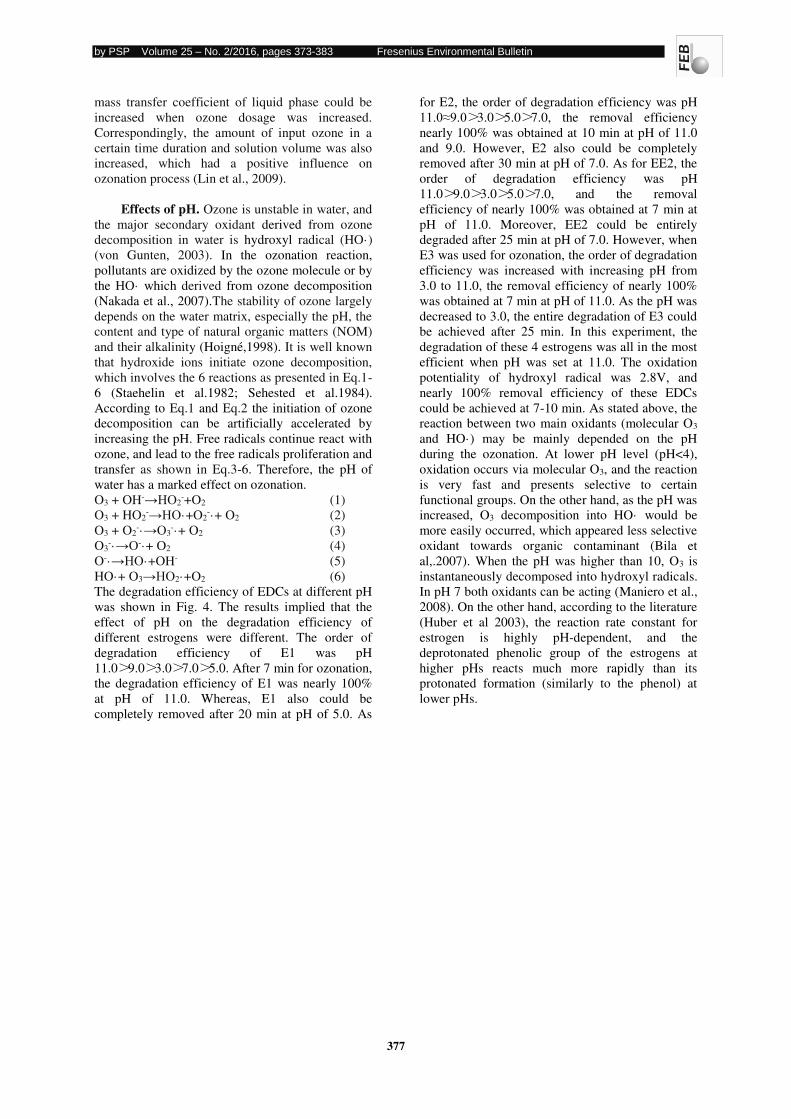
The degradation efficiency of EDCs at different pH
was shown in Fig. 4. The results implied that the
effect of pH on the degradation efficiency of
different estrogens were different. The order of
degradation efficiency of E1 was pH
11.0>9.0>3.0>7.0>5.0. After 7 min for ozonation,
the degradation efficiency of E1 was nearly 100%
at pH of 11.0. Whereas, E1 also could be
completely removed after 20 min at pH of 5.0. As
for E2, the order of degradation efficiency was pH
11.0≈9.0>3.0>5.0>7.0, the removal efficiency
nearly 100% was obtained at 10 min at pH of 11.0
and 9.0. However, E2 also could be completely
removed after 30 min at pH of 7.0. As for EE2, the
order of degradation efficiency was pH
11.0>9.0>3.0>5.0>7.0, and the removal
efficiency of nearly 100% was obtained at 7 min at
pH of 11.0. Moreover, EE2 could be entirely
degraded after 25 min at pH of 7.0. However, when
E3 was used for ozonation, the order of degradation
efficiency was increased with increasing pH from
3.0 to 11.0, the removal efficiency of nearly 100%
was obtained at 7 min at pH of 11.0. As the pH was
decreased to 3.0, the entire degradation of E3 could
be achieved after 25 min. In this experiment, the
degradation of these 4 estrogens was all in the most
efficient when pH was set at 11.0. The oxidation
potentiality of hydroxyl radical was 2.8V, and
nearly 100% removal efficiency of these EDCs
could be achieved at 7-10 min. As stated above, the
reaction between two main oxidants (molecular O3
and HO·) may be mainly depended on the pH
during the ozonation. At lower pH level (pH<4),
oxidation occurs via molecular O3, and the reaction
is very fast and presents selective to certain
functional groups. On the other hand, as the pH was
increased, O3 decomposition into HO· would be
more easily occurred, which appeared less selective
oxidant towards organic contaminant (Bila et
al,.2007). When the pH was higher than 10, O3 is
instantaneously decomposed into hydroxyl radicals.
In pH 7 both oxidants can be acting (Maniero et al.,
2008). On the other hand, according to the literature
(Huber et al 2003), the reaction rate constant for
estrogen is highly pH-dependent, and the
deprotonated phenolic group of the estrogens at
higher pHs reacts much more rapidly than its
protonated formation (similarly to the phenol) at
lower pHs.
by PSP Volume 25 – No. 2/2016, pages 373-383 Fresenius Environmental Bulletin
378
FIGURE 4
Effect of pH on the degradation efficiency of EDCs (2 mg·L-1)
During the ozonation, the difference of
degradation efficiency of these 4 estrogens at same
pH was compared, and the results were shown in
Fig. 4. When pH was at 3.0, the order of
degradation efficiency was as E2>E1>EE2>E3.
The degradation efficiency of E2 could reach to
100% after 10 min treatment, and only 89.4%,
87.8% and 47.1% degradation was observed in E1,
EE2 and E3, respectively. When the pH was set at
5.0, the degradation of E1 and E2 was higher than
that of EE2 and E3, and the removal of E1, E2,
EE2, E3 in 10 min were 79.5%, 79.2%, 65.2% and
64.9%, respectively. The pH was adjusted to 7.0,
the degradation efficiency could be ordered as
E1>E3>EE2>E2, after 10 min treatment, the
removal of E1, E2, EE2, E3 was 87.2%,37.
7.2%,56.4% and 81.0%, respectively. While the pH
was maintained at 9 and 11, all these 4 estrogens
could be degraded very fast, and the difference in
removal of 4 estrogens was not obvious, and a
complete removal of estrogen was achieved at 10
min at pH of 11. According to the obtained results
from Huber et al. (2003), molecular ozone is the
predominant form in pH 3, which is selective to
react with some specific functional groups, such as
activated aromatic systems (i.e., phenolics), amino
groups or double bonds (Harrisson, 2000; von
Gunten, 2003).In this work, comparing 4 estrogens,
as an electron donor group, phenolic ring of E2 can
be rather interesting in reacting with ozone. On the
other hand, the hydroxyl radical is the predominant
oxidant at pH of 11, and the high oxidation rate
constants via HO· indicate that the removal of
EDCs by these oxidants is very fast without
selectivity (von Gunten, 2003; Bila et al,.2007).
Based on this reason, 4 estrogens can be
indiscriminately and thoroughly oxidized.
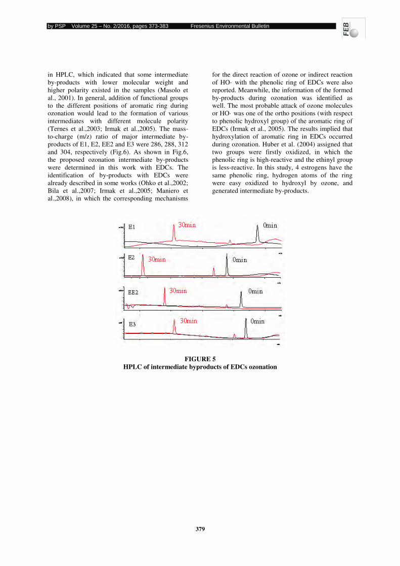
The by-products of ECDs ozonation. The
analysis of by-products during the degradation of
ECDs was conducted by HPLC (Fig. 5). The EDCs
decreased gradually by ozonation and the
intermediate by-products also increased
correspondingly. Comparing with estrogenic
compounds, the ozonation by-products have earlier
retention times in polar eluent (acetonitrile/water)
0 10 20 30
0.0
0.2
0.4
0.6
0.8
1.0
C/C
0 (
%)
Time (min)
pH 3.0
pH 5.0
pH 7.0
pH 9.0
pH11.0
E1
0 10 20 30
0.0
0.2
0.4
0.6
0.8
1.0
C/C
0 (
%)
Time (min)
pH 3.0
pH 5.0
pH 7.0
pH 9.0
pH 11.0
E2
0 10 20 30
0.0
0.2
0.4
0.6
0.8
1.0
C/C
0 (
%)
Time (min)
pH 3.0
pH 5.0
pH 7.0
pH 9.0
pH 11.0
EE2
0 10 20 30
0.0
0.2
0.4
0.6
0.8
1.0
C/C
0 (%
)
Time (min)
pH 3.0
pH 5.0
pH 7.0
pH 9.0
pH 11.0
E3
by PSP Volume 25 – No. 2/2016, pages 373-383 Fresenius Environmental Bulletin
379
in HPLC, which indicated that some intermediate
by-products with lower molecular weight and
higher polarity existed in the samples (Masolo et
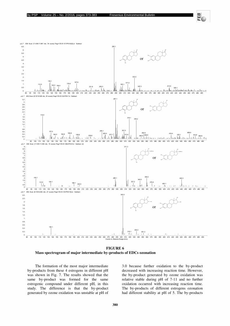
al., 2001). In general, addition of functional groups
to the different positions of aromatic ring during
ozonation would lead to the formation of various
intermediates with different molecule polarity
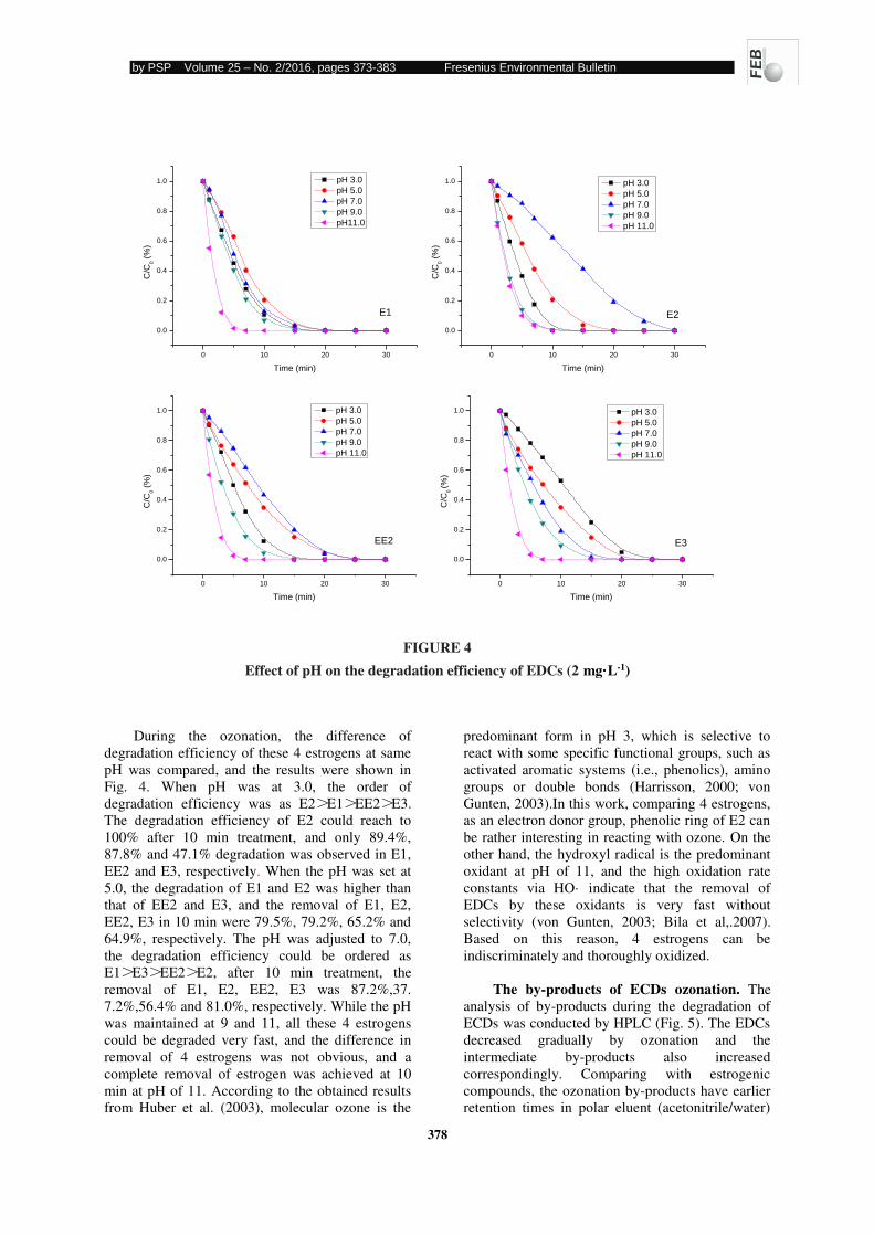
(Ternes et al.,2003; Irmak et al.,2005). The mass-
to-charge (m/z) ratio of major intermediate by-
products of E1, E2, EE2 and E3 were 286, 288, 312
and 304, respectively (Fig.6). As shown in Fig.6,
the proposed ozonation intermediate by-products
were determined in this work with EDCs. The
identification of by-products with EDCs were
already described in some works (Ohko et al.,2002;
Bila et al.,2007; Irmak et al.,2005; Maniero et
al.,2008), in which the corresponding mechanisms
for the direct reaction of ozone or indirect reaction
of HO· with the phenolic ring of EDCs were also
reported. Meanwhile, the information of the formed
by-products during ozonation was identified as
well. The most probable attack of ozone molecules
or HO· was one of the ortho positions (with respect
to phenolic hydroxyl group) of the aromatic ring of
EDCs (Irmak et al., 2005). The results implied that
hydroxylation of aromatic ring in EDCs occurred
during ozonation. Huber et al. (2004) assigned that
two groups were firstly oxidized, in which the
phenolic ring is high-reactive and the ethinyl group
is less-reactive. In this study, 4 estrogens have the
same phenolic ring, hydrogen atoms of the ring
were easy oxidized to hydroxyl by ozone, and
generated intermediate by-products.
FIGURE 5 HPLC of intermediate byproducts of EDCs ozonation
by PSP Volume 25 – No. 2/2016, pages 373-383 Fresenius Environmental Bulletin
380
3x10
0
0.5
1
1.5
2
2.5
3
3.5
4
4.5
5
5.5
6
6.5
-ESI Scan (11.638-11.881 min, 34 scans) Frag=135.0V E1-PH3-5(02).d Subtract
285.1
333.0
136.1197.8 317.2
179.9112.9 305.1144.0 156.0 413.9345.3255.3231.8
429.1
Counts vs. Mass-to-Charge (m/ z)
80 90 100 110 120 130 140 150 160 170 180 190 200 210 220 230 240 250 260 270 280 290 300 310 320 330 340 350 360 370 380 390 400 410 420 430 440 450 460 470 480 490
3x10
0
0.2
0.4
0.6
0.8
1
1.2
1.4
1.6
1.8
2
2.2
2.4
2.6
2.8
3
3.2
-ESI Scan (8.167-8.528 min, 50 scans) Frag=135.0V E2-PH5-7.d Subtract
287.1
116.9
319.1335.2
307.0255.1137.2458.9352.9180.8 263.0 416.4164.8146.9 313.0277.1199.8 435.1 472.8358.9228.8 346.9 484.8
Counts vs. Mass-to-Charge (m/ z)
90 100 110 120 130 140 150 160 170 180 190 200 210 220 230 240 250 260 270 280 290 300 310 320 330 340 350 360 370 380 390 400 410 420 430 440 450 460 470 480 490
3x10
0
0.5
1
1.5
2
2.5
3
3.5
4
4.5
5
5.5
6
6.5
7
7.5
8
8.5
9
-ESI Scan (11.535-11.638 min, 15 scans) Frag=135.0V EE2-PH3-5.d Subtract (2)
311.3
359.0100.1 285.1 440.3343.0
327.2135.1112.9 370.9189.1 400.1202.0
Counts vs. Mass-to-Charge (m/ z)
80 90 100 110 120 130 140 150 160 170 180 190 200 210 220 230 240 250 260 270 280 290 300 310 320 330 340 350 360 370 380 390 400 410 420 430 440 450 460 470 480 490
4x10
0
0.2
0.4
0.6
0.8
1
1.2
1.4
1.6
1.8
2
2.2
2.4
-ESI Scan (8.100-8.292 min, 27 scans) Frag=135.0V E3-PH5-7(2).d Subtract
303.3
136.1
335.3319.1 351.3
Counts vs. Mass-to-Charge (m/ z)
80 90 100 110 120 130 140 150 160 170 180 190 200 210 220 230 240 250 260 270 280 290 300 310 320 330 340 350 360 370 380 390 400 410 420 430 440 450 460 470 480 490
HO
O
OH
HO
OH
O
or
HO
OH
OH
HO
OH
OH
or
HO
OH
OH
C CH
HO
OH
OH
C CH
or
HO
OH
OH
OH
HO
OH
OH
OH
or
FIGURE 6
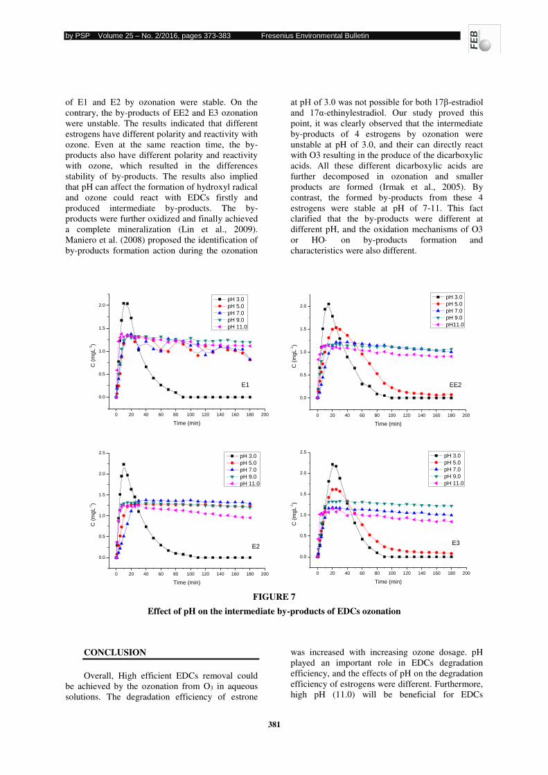
Mass spectrogram of major intermediate by-products of EDCs ozonation The formation of the most major intermediate
by-products from these 4 estrogens in different pH
was shown in Fig. 7. The results showed that the
same by-product was formed for the same
estrogenic compound under different pH, in this
study. The difference is that the by-product
generated by ozone oxidation was unstable at pH of
3.0 because further oxidation to the by-product
decreased with increasing reaction time. However,
the by-product generated by ozone oxidation was
relative stable during pH of 7-11 and no further
oxidation occurred with increasing reaction time.
The by-products of different estrogens ozonation
had different stability at pH of 5. The by-products
by PSP Volume 25 – No. 2/2016, pages 373-383 Fresenius Environmental Bulletin
381
of E1 and E2 by ozonation were stable. On the
contrary, the by-products of EE2 and E3 ozonation
were unstable. The results indicated that different
estrogens have different polarity and reactivity with
ozone. Even at the same reaction time, the by-
products also have different polarity and reactivity
with ozone, which resulted in the differences
stability of by-products. The results also implied
that pH can affect the formation of hydroxyl radical
and ozone could react with EDCs firstly and
produced intermediate by-products. The by-
products were further oxidized and finally achieved
a complete mineralization (Lin et al., 2009).
Maniero et al. (2008) proposed the identification of
by-products formation action during the ozonation
at pH of 3.0 was not possible for both 17β-estradiol
and 17α-ethinylestradiol. Our study proved this
point, it was clearly observed that the intermediate
by-products of 4 estrogens by ozonation were
unstable at pH of 3.0, and their can directly react
with O3 resulting in the produce of the dicarboxylic
acids. All these different dicarboxylic acids are
further decomposed in ozonation and smaller
products are formed (Irmak et al., 2005). By
contrast, the formed by-products from these 4
estrogens were stable at pH of 7-11. This fact
clarified that the by-products were different at
different pH, and the oxidation mechanisms of O3
or HO· on by-products formation and
characteristics were also different.
FIGURE 7
Effect of pH on the intermediate by-products of EDCs ozonation
CONCLUSION
Overall, High efficient EDCs removal could
be achieved by the ozonation from O3 in aqueous
solutions. The degradation efficiency of estrone
was increased with increasing ozone dosage. pH
played an important role in EDCs degradation
efficiency, and the effects of pH on the degradation
efficiency of estrogens were different. Furthermore,
high pH (11.0) will be beneficial for EDCs
0 20 40 60 80 100 120 140 160 180 200
0.0
0.5
1.0
1.5
2.0
C (
mg
L-1)
Time (min)
pH 3.0
pH 5.0
pH 7.0
pH 9.0
pH 11.0
E1
0 20 40 60 80 100 120 140 160 180 200
0.0
0.5
1.0
1.5
2.0
2.5
C (
mg
L-1)
Time (min)
pH 3.0
pH 5.0
pH 7.0
pH 9.0
pH 11.0
E2
0 20 40 60 80 100 120 140 160 180 200
0.0
0.5
1.0
1.5
2.0
C (
mg
L-1)
Time (min)
pH 3.0
pH 5.0
pH 7.0
pH 9.0
pH11.0
EE2
0 20 40 60 80 100 120 140 160 180 200
0.0
0.5
1.0
1.5
2.0
2.5
C (
mg
L-1)
Time (min)
pH 3.0
pH 5.0
pH 7.0
pH 9.0
pH 11.0
E3
by PSP Volume 25 – No. 2/2016, pages 373-383 Fresenius Environmental Bulletin
382
degradation. The oxidation process of EDCs was
analyzed by HPLC, indicating hydrogen atoms of
the phenolic ring were easily oxidized to hydroxyl
by ozone, which was the main route to form the
intermediate by-products. However, only a few
compounds could be proposed and needed to be
confirmed in future work.
ACKNOWLEDGEMENTS
This work was supported by Jiangsu province
Natural Science Foundation of China
(BK20131271), National Hightech R&D Program
of China (Grant no. 2013AA06A309). We thanks
Dr. Gong Huijuan in the Center of Materials
Analysis of Nanjing University for her assistance
for analysis of by-products using HPLC-MS.
REFERENCES
[1] M. Auriol, Y. Filali-Meknassi, R.D. Tyagi,
C.D. Adams, R.Y. Surampalli, (2006)
Endocrine disrupting compounds removal
from wastewater, a new challenge, Process.
Biochem. 41:525–539.
[2] H. Bader, J. Hoigné, (1981) Determination of
ozone in water by the indigo method, Water
Res. 15:449-456.
[3] D. Bila, A.F.Montalvão, D.Azevedo,
M.Dezotti, (2007)Estrogenic activity removal
of 17β-estradiol by ozonation and
identification of by-products, Chemosphere,
69:736–746
[4] J.V. Brett, A. P. Rebecca, J. R. David,
A.S.Shane, (2003) Analysis of endocrine
disruptors, pharmaceuticals, and personal care
products in water using liquid
chromatography/tandem mass spectrometry,
Anal. Chem., 75:6265–6274
[5] Y.H. Han, K. Ichikawa, H. Utsumi, (2004) A
kinetic study of enhancing effect by phenolic
compounds on the hydroxyl radical generation
during ozonation, Water Sci.Technol. 50:97–102.
[6] J.F. Harrisson, Ozone for Point-of Use, Point-
of-Entry, and Small Water System Water
Treatment Applications – A Reference
Manual, Water Quality Association, Lisle.
2000
[7] J. Hoigné, Chemistry of aqueous ozone, and
transformation of pollutants by ozonation and
advanced oxidation processes, In: J. Hubrec,
editor. The handbook of environmental
chemistry quality and treatment of drinking
water, Berlin: Springer, 1998
[8] S. Irmak, O. Erbatur, A. Akgerman, (2005)
Degradation of 17β-estradiol and bisphenol A
in aqueous medium by using ozone and
ozone/UV techniques, Journal of Hazardous
Materials. B126: 54–62
[9] U. Kepa, E. Stanczyk-Mazanek, L. Stepniak,
(2008) The use of the advanced oxidation
process in the ozone + hydrogen peroxide
system for the removal of cyanide from water,
Desalination. 223:187-193.
[10] B.H. Lee, W.C. Song, B. Manna, J.K. Ha,
(2008) Dissolved ozone flotation (DOF)-a
promising technology in municipal wastewater
treatment, Desalination.225:260–273.
[11] Y.X. Lin, Z.G. Peng, X. Zhang, (2009)
Ozonation of estrone, estradiol,
diethylstilbestrol in waters, Desalination. 249:
235-240
[12] M.M. Huber, S. Canonica, G.U. Park, U. von
Gunten, (2003) Oxidation of Pharmaceuticals
during Ozonation and Advanced Oxidation
Processes, Environ. Sci. Technol. 37:1016-
1024.
[13] M.M.Huber, T.A.Ternes, U.von Gunten,
(2004) Removal of Estrogenic Activity and
Formation of Oxidation Products during
Ozonation of 17α-Ethinylestradiol, Environ.
Sci. Technol. 38:5177–5186
[14] G. Masolo, A. Lopez, H. James, M. Fielding,
(2001)By-products formation during
degradation of isoproturon in aqueous
solution, Ozonation, Water Res. 35:1695–1704.
[15] M.G. Maniero, D.M. Bila, M. Dezotti, (2008)
Degradation and estrogenic activity removal
of 17β-estradiol and 17α-ethinylestradiol by
ozonation and O3/H2O2,Science of the Total
Environment. 407:105-115
[16] N. Nakada, H. Shinohara, A. Murata, K. Kiri,
S. Anagaki, N. Sato, H. Takada,
(2007)Removal of selected pharmaceuticals
and personal care products (PPCPs) and
endocrine disrupting chemicals (EDCs) during
sand filtration and ozonation at a municipal
sewage treatment plant, Water. Res. 41:4373-
4382
[17] T. Ölmez -Hanci, I. Kabdash, O. Tunay, C.
Imren, D. Gulhan, (2012)Treatment of
aqueous dimethyl phythalate solution by
fenton and photo-fenton processes, Fresenius
Environmental Bulletin. 21(10A):3136-3141
[18] Y. Ohko, K. Iuchi, C. Niwa, T. Tatsuma, T.
Nakashima, T. Iguchi, Y. Kubota, A.
Fujishima, (2002)17β-estradiol degradation by
TiO2 photocatalysis as a means of reducing
by PSP Volume 25 – No. 2/2016, pages 373-383 Fresenius Environmental Bulletin
383
estrogenic activity, Environ Sci Technol .
36:4175–4181.
[19] R.O. Pereira, C. Postigo, M. López de Alda,
L.A. Daniel, D. Barceló, (2011) Removal of
estrogens through water disinfection processes
and formation of by-products,
Chemosphere.82:789–799
[20] M.S. Rodriguez, J. Marίa, M. Lόpez de Alda,
D. Barcelό, (2004) Monitoring of estrogens, pesticides and bisphenol A in natural waters
and drinking water treatment plants by solid-
phase extraction-liquid chromatography-mass
spectrometry, J. Chromatogr.A 1045:85–92.
[21] E.J. Routledge, D. Sheahan, C.Desbrow,
G.C.Brighty, M.Waldock, J.P. Sumpter,
(1998) Identification of estrogenic chemicals
in STW effluent. 2. In vivo responses in trout
and roach, Environ. Sci. Technol. 32:1559–1565.
[22] K. Sehested, J. Holcman, E. Bjergbakke, E.J.
Hart, (1984):Formation of ozone in the
reaction of O3- and the decay of the ozonide
ion radical at pH 10–13, J Phys Chem.88269–273.
[23] J.Staehelin, J. Hoigné, (1982) Decomposition
of ozone in water:rate of initiation by
hydroxide ions and hydrogen peroxide,
Environ Sci Technol.16:676–681.
[24] T.A. Ternes, M. Stumph, J. Mueller, H.
Haberer, R.D. Wilken, M. Servos, (1999)
Behavior and occurrence of estrogens in
municipal sewage treatment plants-I.
Investigations in Germany, Canada and Brazil,
Sci Total Environ.225:81–90.
[25] T.A.Ternes, J.Stüber, N.Hermann,
D.McDowell, A.Ried, M. Kampmann,
B.Teiser, (2003) Ozonation: a tool for removal
of pharmaceuticals, contrast media and musk
fragrances from wastewater? Water Res.
37:1976–1982.
[26] U.von Gunten, Ozonation of drinking water:
part I. Oxidation kinetics and product
formation. Water Res. 37 (2003):1443–1467.
[27] J. N. Wu, T.W. Wang, (2001) Ozonation of
aqueous azo dye in a semi-batch reactor,
Water. Res.35:1093-1099
[28] Y. Zhang, J.L. Zhou, (2008) Occurrence and
removal of endocrine disrupting chemicals in
wastewater, Chemosphere. 73:848–853
[29] W.L. Zhang, Y Li, K Mao. G.P.
Li,(2012)Removal of endocrine disrupting
compounds and estrogenic activity from
secondary effluents during TiO2
photocatalysis. Fresenius Environmental
Bulletin. 21(3A):731-73
[30] G. Zuo, Y.J. Lin, (2007) Solvent effects on the
silylation-gas chromatography-mass
spectrometric determination of natural and
synthetic estreogenic silylation-gas
chromatography-mass spectrometric
determination of natural and synthetic
estrogenic steroid hormones: Comment on
“Formation of chlorinated estrones via hypochlorous disinfection of wastewater
effluent containing estrone”, Chemosphere. 69:1175–1176,
Received: 06.03.2015 Accepted: 04.12.2015 CORRESPONDING AUTHOR
Dr. X. Qiming Nanjing University
Environmental Analytical Chemistry Laboratory
163 Xianlin Avenue
Nanjing, 210046 - P. R. China
E-mail address: [email protected]
by PSP Volume 25 – No. 2/2016, pages 384-390 Fresenius Environmental Bulletin
384
INDUSTRIAL EXPERIMENTAL STUDY ON SO2 REMOVAL
DURING NOVEL INTEGRATED SINTERING FLUE GAS
DESULFURIZATION PROCESS
Qin Linbo1, Han Jun1, Deng Yurui1, He Chao1, Chen Wangsheng1
1College of Resources and Environment Engineering, Wuhan University of Science and Technology, Wuhan 430081, Hubei, China
ABSTRACT
In order to increase the desulfurization
efficiency and sorbent utilization of the novel
integrated sintering flue gas desulfurization system,
industrial experiments in a commercial-scale novel
integrated desulfurization(NID) system were
conducted to investigate the effects of operating
parameters (inlet SO2 concentration, inlet gas
temperature, CaO/S, H2O/CaO) on SO2 removal
efficiency and the outlet SO2 concentration. The
commercial-scale experimental results confirmed
that the SO2 removal efficiency in excess of 96%
was achieved by optimizing the operating
parameters. The SO2 removal efficiency was
increased with the gas temperature enhancement.
Much lower and higher inlet SO2 concentration and
H2O/CaO adversely influenced SO2 removal
efficiency. Larger CaO/S was greatly increased the
SO2 removal efficiency but a further increase can
not effectively affect SO2 removal efficiency.
KEYWORDS:
Novel integrated desulfurization; Industrial experiments;
Sintering flue gas
INTRODUCTION
In China, the sintering process of iron ore
annually emitted about 1.5 million tons of SO2,
which occupied 70% SO2 produced from iron and
steel industry [1]. With the implementation of new
acts or regulations, SO2 emission from the sintering
process has received wide attention. “Discharge standard of air pollutants for iron and steel
industry” requires that SO2 emission from the
sintering process of iron ore must be below 200
mg/Nm3 since 2013 [2, 3]. In order to meet
availability requirements and stringent standards of
SO2 removal, the iron and steel companies make
every effort to construct flue gas desulfurization
system for removing SO2 [4, 5, 6, 7].
Novel Integrated Desulfurization (NID)
technology is one of an effectively semi-dry flue
gas desulfurization, which was widely used in
medium- and small-scale flue gas desulfurization
with the advantages of small space requirement,
low water consumption, low investment and
operation costs [8, 9, 10, 11]. Since the first NID
system was imported from Alstom Company in
1998, more than 100 sets of NID system are
constructed for coal-fired power flue gas
desulfurization in China [12]. As for novel
integrated sintering flue gas desulfurization, the
first novel integrated sintering flue gas
desulfurization system was constructed in the
572m2 sintering device of France’ SOLLAC steel company in 2005, and confirmed that the
desulfurization efficiency was above 50% [13]. In
2009, the NID technology was imported from
Alstom Company, and constructed in 360m2
sintering device of Wuhan iron and steel company.
The operation results demonstrated that SO2
removal efficiency in excess of 80% can be
achieved, while it has shortcomings of high sorbent
utilization and poor stability. Above all, the SO2
emission concentration can not meet environmental
regulation when the inlet SO2 concentration was
above 2000 mg/m3 [14].
In order to increase the desulfurization
efficiency and sorbent utilization of the novel
integrated sintering flue gas desulfurization system,
the effects of operating parameters (Inlet SO2
concentration, inlet gas temperature, CaO/S,
H2O/CaO) on the SO2 removal efficiency and the
outlet SO2 concentration were investigated in a
commercial-scale novel integrated desulfurization
(NID) system.
MATERIALS AND METHODS
Materials. In the experiments, lime was used
as sorbent and stored in the slurry tank after
hydration. Sauter diameter of the lime slurry is
~74μm. Chemical and physical characteristics of sorbent are presented in Tab.1.
by PSP Volume 25 – No. 2/2016, pages 384-390 Fresenius Environmental Bulletin
385
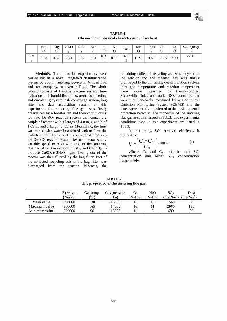
TABLE 1
Chemical and physical characteristics of sorbent
Na2
O
Mg
O
Al2O
3
SiO
2
P2O
5 SO3
K2
O CaO
Mn
O
Fe2O
3
Cu
O
Zn
O
SBET/(m3/g
)
Lim
e 3.58 0.59 0.74 1.09 1.14
0.3
7 0.17
87.0
1 0.21 0.63 1.15 3.33
22.16
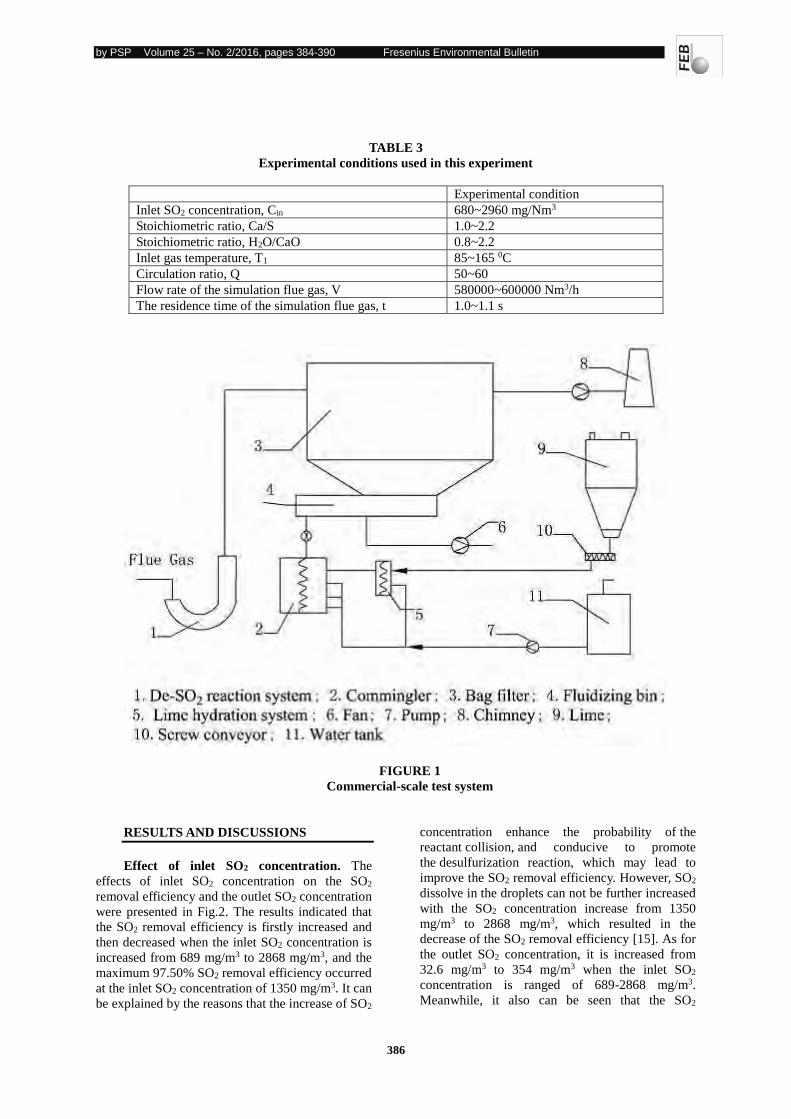
Methods. The industrial experiments were
carried out in a novel integrated desulfurization
system of 360m2 sintering device in Wuhan iron
and steel company, as given in Fig.1. The whole
facility consists of De-SO2 reaction system, lime
hydration and humidification system, ash feeding
and circulating system, ash conveying system, bag
filter and data acquisition system. In this
experiment, the sintering flue gas was firstly
pressurized by a booster fan and then continuously
fed into De-SO2 reaction system that contains a
couple of reactor with a length of 4.0 m, a width of
1.65 m, and a height of 22 m. Meanwhile, the lime
was mixed with water in a stirred tank to form the
hydrated lime that was also continuously fed into
the De-SO2 reaction system by an injector with a
variable speed to react with SO2 of the sintering
flue gas. After the reaction of SO2 and Ca(OH)2 to
produce CaSO4 2H2O, gas flowing out of the
reactor was then filtered by the bag filter. Part of
the collected recycling ash in the bag filter was
discharged from the reactor. Whereas, the
remaining collected recycling ash was recycled to
the reactor and the cleaned gas was finally
discharged to the air. In this desulfurization system,
inlet gas temperature and reaction temperature
were online measured by thermocouples.
Meanwhile, inlet and outlet SO2 concentrations
were simultaneously measured by a Continuous
Emission Monitoring System (CEMS) and the
dates were directly transferred to the environmental
protection network. The properties of the sintering
flue gas are summarized in Tab.2. The experimental
conditions used in this experiment are listed in
Tab.3.
In this study, SO2 removal efficiency is
defined as
100%in out
in
C C
C
(1)
Where, Cin and Cout are the inlet SO2
concentration and outlet SO2 concentration,
respectively.
TABLE 2
The propertied of the sintering flue gas
Flow rate
(Nm3/h)
Gas temp.
(0C)
Gas pressure
(Pa)
O2
(Vol %)
H2O
(Vol %)
SO2
(mg/Nm3)
Dust
(mg/Nm3)
Mean value 590000 130 -15000 15 10 1560 80
Maximum value 600000 165 -14000 16 11 2960 150
Minimum value 580000 90 -16000 14 9 680 50
by PSP Volume 25 – No. 2/2016, pages 384-390 Fresenius Environmental Bulletin
386
TABLE 3
Experimental conditions used in this experiment
Experimental condition
Inlet SO2 concentration, Cin 680~2960 mg/Nm3
Stoichiometric ratio, Ca/S 1.0~2.2
Stoichiometric ratio, H2O/CaO 0.8~2.2
Inlet gas temperature, T1 85~165 0C
Circulation ratio, Q 50~60
Flow rate of the simulation flue gas, V 580000~600000 Nm3/h
The residence time of the simulation flue gas, t 1.0~1.1 s
FIGURE 1
Commercial-scale test system
RESULTS AND DISCUSSIONS
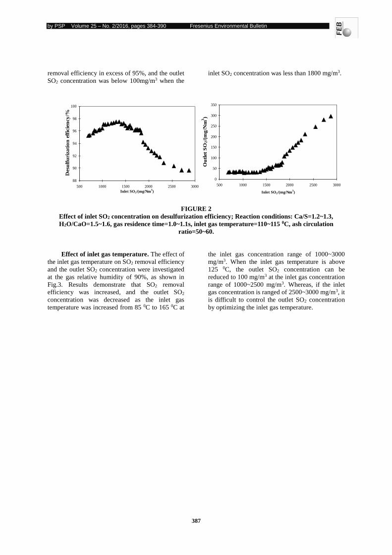
Effect of inlet SO2 concentration. The
effects of inlet SO2 concentration on the SO2
removal efficiency and the outlet SO2 concentration
were presented in Fig.2. The results indicated that
the SO2 removal efficiency is firstly increased and
then decreased when the inlet SO2 concentration is
increased from 689 mg/m3 to 2868 mg/m3, and the
maximum 97.50% SO2 removal efficiency occurred
at the inlet SO2 concentration of 1350 mg/m3. It can
be explained by the reasons that the increase of SO2
concentration enhance the probability of the
reactant collision, and conducive to promote
the desulfurization reaction, which may lead to
improve the SO2 removal efficiency. However, SO2
dissolve in the droplets can not be further increased
with the SO2 concentration increase from 1350
mg/m3 to 2868 mg/m3, which resulted in the
decrease of the SO2 removal efficiency [15]. As for
the outlet SO2 concentration, it is increased from
32.6 mg/m3 to 354 mg/m3 when the inlet SO2
concentration is ranged of 689-2868 mg/m3.
Meanwhile, it also can be seen that the SO2
by PSP Volume 25 – No. 2/2016, pages 384-390 Fresenius Environmental Bulletin
387
removal efficiency in excess of 95%, and the outlet
SO2 concentration was below 100mg/m3 when the
inlet SO2 concentration was less than 1800 mg/m3.
FIGURE 2
Effect of inlet SO2 concentration on desulfurization efficiency; Reaction conditions: Ca/S=1.2~1.3,
H2O/CaO=1.5~1.6, gas residence time=1.0~1.1s, inlet gas temperature=110~115 0C, ash circulation
ratio=50~60.
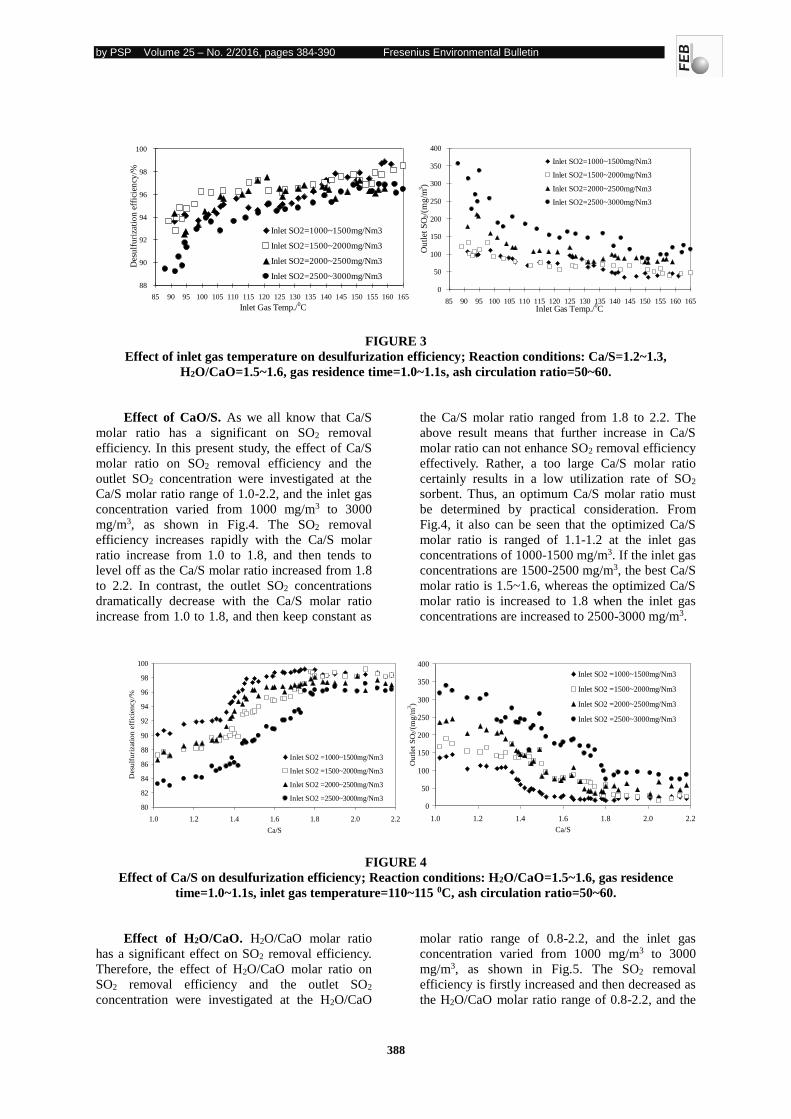
Effect of inlet gas temperature. The effect of
the inlet gas temperature on SO2 removal efficiency
and the outlet SO2 concentration were investigated
at the gas relative humidity of 90%, as shown in
Fig.3. Results demonstrate that SO2 removal
efficiency was increased, and the outlet SO2
concentration was decreased as the inlet gas
temperature was increased from 85 0C to 165 0C at
the inlet gas concentration range of 1000~3000
mg/m3. When the inlet gas temperature is above
125 0C, the outlet SO2 concentration can be
reduced to 100 mg/m3 at the inlet gas concentration
range of 1000~2500 mg/m3. Whereas, if the inlet
gas concentration is ranged of 2500~3000 mg/m3, it
is difficult to control the outlet SO2 concentration
by optimizing the inlet gas temperature.
88
90
92
94
96
98
100
500 1000 1500 2000 2500 3000
Inlet SO2/(mg/Nm3)
Des
ulf
uri
zati
on
eff
icie
ncy
/%
0
50
100
150
200
250
300
350
500 1000 1500 2000 2500 3000
Inlet SO2/(mg/Nm3)
Ou
tlet
SO
2/(
mg
/Nm
3)
by PSP Volume 25 – No. 2/2016, pages 384-390 Fresenius Environmental Bulletin
388
FIGURE 3
Effect of inlet gas temperature on desulfurization efficiency; Reaction conditions: Ca/S=1.2~1.3,
H2O/CaO=1.5~1.6, gas residence time=1.0~1.1s, ash circulation ratio=50~60.
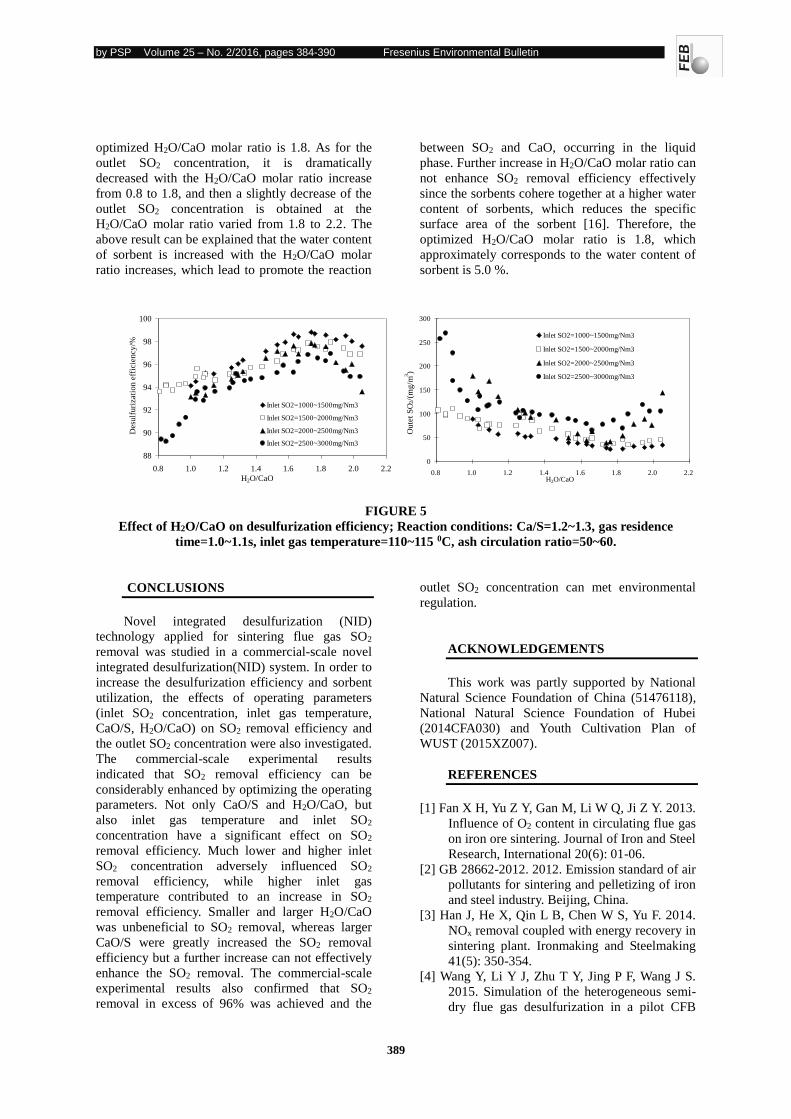
Effect of CaO/S. As we all know that Ca/S
molar ratio has a significant on SO2 removal
efficiency. In this present study, the effect of Ca/S
molar ratio on SO2 removal efficiency and the
outlet SO2 concentration were investigated at the
Ca/S molar ratio range of 1.0-2.2, and the inlet gas
concentration varied from 1000 mg/m3 to 3000
mg/m3, as shown in Fig.4. The SO2 removal
efficiency increases rapidly with the Ca/S molar
ratio increase from 1.0 to 1.8, and then tends to
level off as the Ca/S molar ratio increased from 1.8
to 2.2. In contrast, the outlet SO2 concentrations
dramatically decrease with the Ca/S molar ratio
increase from 1.0 to 1.8, and then keep constant as
the Ca/S molar ratio ranged from 1.8 to 2.2. The
above result means that further increase in Ca/S
molar ratio can not enhance SO2 removal efficiency
effectively. Rather, a too large Ca/S molar ratio
certainly results in a low utilization rate of SO2
sorbent. Thus, an optimum Ca/S molar ratio must
be determined by practical consideration. From
Fig.4, it also can be seen that the optimized Ca/S
molar ratio is ranged of 1.1-1.2 at the inlet gas
concentrations of 1000-1500 mg/m3. If the inlet gas
concentrations are 1500-2500 mg/m3, the best Ca/S
molar ratio is 1.5~1.6, whereas the optimized Ca/S
molar ratio is increased to 1.8 when the inlet gas
concentrations are increased to 2500-3000 mg/m3.
FIGURE 4
Effect of Ca/S on desulfurization efficiency; Reaction conditions: H2O/CaO=1.5~1.6, gas residence
time=1.0~1.1s, inlet gas temperature=110~115 0C, ash circulation ratio=50~60.
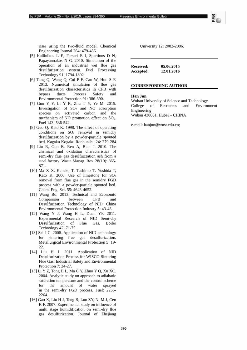
Effect of H2O/CaO. H2O/CaO molar ratio
has a significant effect on SO2 removal efficiency.
Therefore, the effect of H2O/CaO molar ratio on
SO2 removal efficiency and the outlet SO2
concentration were investigated at the H2O/CaO
molar ratio range of 0.8-2.2, and the inlet gas
concentration varied from 1000 mg/m3 to 3000
mg/m3, as shown in Fig.5. The SO2 removal
efficiency is firstly increased and then decreased as
the H2O/CaO molar ratio range of 0.8-2.2, and the
80
82
84
86
88
90
92
94
96
98
100
1.0 1.2 1.4 1.6 1.8 2.0 2.2
Ca/S
Des
ulf
uri
zati
on
eff
icie
ncy
/%
Inlet SO2 =1000~1500mg/Nm3
Inlet SO2 =1500~2000mg/Nm3
Inlet SO2 =2000~2500mg/Nm3
Inlet SO2 =2500~3000mg/Nm30
50
100
150
200
250
300
350
400
1.0 1.2 1.4 1.6 1.8 2.0 2.2
Ca/S
Outl
et
SO
2/(
mg/m
3)
Inlet SO2 =1000~1500mg/Nm3
Inlet SO2 =1500~2000mg/Nm3
Inlet SO2 =2000~2500mg/Nm3
Inlet SO2 =2500~3000mg/Nm3
88
90
92
94
96
98
100
85 90 95 100 105 110 115 120 125 130 135 140 145 150 155 160 165
Inlet Gas Temp./0C
Des
ulf
uri
zati
on
eff
icie
ncy
/%
Inlet SO2=1000~1500mg/Nm3
Inlet SO2=1500~2000mg/Nm3
Inlet SO2=2000~2500mg/Nm3
Inlet SO2=2500~3000mg/Nm3
0
50
100
150
200
250
300
350
400
85 90 95 100 105 110 115 120 125 130 135 140 145 150 155 160 165Inlet Gas Temp./
0C
Ou
tlet
SO
2/(
mg
/m3)
Inlet SO2=1000~1500mg/Nm3
Inlet SO2=1500~2000mg/Nm3
Inlet SO2=2000~2500mg/Nm3
Inlet SO2=2500~3000mg/Nm3
by PSP Volume 25 – No. 2/2016, pages 384-390 Fresenius Environmental Bulletin
389
optimized H2O/CaO molar ratio is 1.8. As for the
outlet SO2 concentration, it is dramatically
decreased with the H2O/CaO molar ratio increase
from 0.8 to 1.8, and then a slightly decrease of the
outlet SO2 concentration is obtained at the
H2O/CaO molar ratio varied from 1.8 to 2.2. The
above result can be explained that the water content
of sorbent is increased with the H2O/CaO molar
ratio increases, which lead to promote the reaction
between SO2 and CaO, occurring in the liquid
phase. Further increase in H2O/CaO molar ratio can
not enhance SO2 removal efficiency effectively
since the sorbents cohere together at a higher water
content of sorbents, which reduces the specific
surface area of the sorbent [16]. Therefore, the
optimized H2O/CaO molar ratio is 1.8, which
approximately corresponds to the water content of
sorbent is 5.0 %.
FIGURE 5
Effect of H2O/CaO on desulfurization efficiency; Reaction conditions: Ca/S=1.2~1.3, gas residence
time=1.0~1.1s, inlet gas temperature=110~115 0C, ash circulation ratio=50~60.
CONCLUSIONS
Novel integrated desulfurization (NID)
technology applied for sintering flue gas SO2
removal was studied in a commercial-scale novel
integrated desulfurization(NID) system. In order to
increase the desulfurization efficiency and sorbent
utilization, the effects of operating parameters
(inlet SO2 concentration, inlet gas temperature,
CaO/S, H2O/CaO) on SO2 removal efficiency and
the outlet SO2 concentration were also investigated.
The commercial-scale experimental results
indicated that SO2 removal efficiency can be
considerably enhanced by optimizing the operating
parameters. Not only CaO/S and H2O/CaO, but
also inlet gas temperature and inlet SO2
concentration have a significant effect on SO2
removal efficiency. Much lower and higher inlet
SO2 concentration adversely influenced SO2
removal efficiency, while higher inlet gas
temperature contributed to an increase in SO2
removal efficiency. Smaller and larger H2O/CaO
was unbeneficial to SO2 removal, whereas larger
CaO/S were greatly increased the SO2 removal
efficiency but a further increase can not effectively
enhance the SO2 removal. The commercial-scale
experimental results also confirmed that SO2
removal in excess of 96% was achieved and the
outlet SO2 concentration can met environmental
regulation.
ACKNOWLEDGEMENTS
This work was partly supported by National
Natural Science Foundation of China (51476118),
National Natural Science Foundation of Hubei
(2014CFA030) and Youth Cultivation Plan of
WUST (2015XZ007).
REFERENCES
[1] Fan X H, Yu Z Y, Gan M, Li W Q, Ji Z Y. 2013.
Influence of O2 content in circulating flue gas
on iron ore sintering. Journal of Iron and Steel
Research, International 20(6): 01-06.
[2] GB 28662-2012. 2012. Emission standard of air
pollutants for sintering and pelletizing of iron
and steel industry. Beijing, China.
[3] Han J, He X, Qin L B, Chen W S, Yu F. 2014.
NOx removal coupled with energy recovery in
sintering plant. Ironmaking and Steelmaking
41(5): 350-354.
[4] Wang Y, Li Y J, Zhu T Y, Jing P F, Wang J S.
2015. Simulation of the heterogeneous semi-
dry flue gas desulfurization in a pilot CFB
88
90
92
94
96
98
100
0.8 1.0 1.2 1.4 1.6 1.8 2.0 2.2
H2O/CaO
Desu
lfuri
zati
on e
ffic
iency/%
Inlet SO2=1000~1500mg/Nm3
Inlet SO2=1500~2000mg/Nm3
Inlet SO2=2000~2500mg/Nm3
Inlet SO2=2500~3000mg/Nm3
0
50
100
150
200
250
300
0.8 1.0 1.2 1.4 1.6 1.8 2.0 2.2H2O/CaO
Oute
t S
O2/(
mg/m
3)
Inlet SO2=1000~1500mg/Nm3
Inlet SO2=1500~2000mg/Nm3
Inlet SO2=2000~2500mg/Nm3
Inlet SO2=2500~3000mg/Nm3
by PSP Volume 25 – No. 2/2016, pages 384-390 Fresenius Environmental Bulletin
390
riser using the two-fluid model. Chemical
Engineering Journal 264: 479-486.
[5] Kallinikos L E, Farsari E I, Spartinos D N,
Papayannakos N G. 2010. Simulation of the
operation of an industrial wet flue gas
desulfurization system. Fuel Processing
Technology 91: 1794-1802.
[6] Tang Q, Wang Q, Cui P F, Cao W, Hou S F.
2013. Numerical simulation of flue gas
desulfurization characteristics in CFB with
bypass ducts. Process Safety and
Environmental Protection 91: 386-390.
[7] Guo Y Y, Li Y R, Zhu T Y, Ye M. 2015.
Investigation of SO2 and NO adsorption
species on activated carbon and the
mechanism of NO promotion effect on SO2.
Fuel 143: 536-542.
[8] Guo Q, Kato K. 1998. The effect of operating
conditions on SO2 removal in semidry
desulfurization by a powder-particle spouted
bed. Kagaku Kogaku Ronbunshu 24: 279-284.
[9] Liu R, Guo B, Ren A, Bian J. 2010. The
chemical and oxidation characteristics of
semi-dry flue gas desulfurization ash from a
steel factory. Waste Manag. Res. 28(10): 865-
871.
[10] Ma X X, Kaneko T, Tashimo T, Yoshida T,
Kato K. 2000. Use of limestone for SO2
removal from flue gas in the semidry FGD
process with a powder-particle spouted bed.
Chem. Eng. Sci. 55: 4643-4652.
[11] Wang Bo. 2013. Technical and Economic
Comparison between CFB and
Desulfurization Technology of NID. China
Environmental Protection Industry 5: 43-48.
[12] Wang Y J, Wang H L, Duan YF. 2011.
Experimental Research of NID Semi-dry
Desulfurization of Flue Gas. Boiler
Technology 42: 71-75.
[13] Sai J C. 2008. Application of NID technology
for sintering flue gas desulfurization.
Metallurgical Environmental Protection 5: 19-
22.
[14] Liu H J. 2011. Application of NID
Desulfurization Process for WISCO Sintering
Flue Gas. Industrial Safety and Environmental
Protection 7: 24-27.
[15] Li Y Z, Tong H L, Ma C Y, Zhuo Y Q, Xu XC.
2004. Analytic study on approach to adiabatic
saturation temperature and the control scheme
for the amount of water sprayed
in the semi-dry FGD process. Fuel: 2255-
2264.
[16] Gao X, Liu H J, Teng B, Luo ZY, Ni M J, Cen
K F. 2007. Experimental study on influence of
multi stage humidification on semi-dry flue
gas desulfurization. Journal of Zhejiang
University 12: 2082-2086.
Received: 05.06.2015
Accepted: 12.01.2016
CORRESPONDING AUTHOR
Han Jun
Wuhan University of Science and Technology
College of Resources and Environment
Engineering
Wuhan 430081, Hubei – CHINA
e-mail: [email protected];
by PSP Volume 25 – No. 2/2016, pages 391-400 Fresenius Environmental Bulletin
391
THE PREPARATION OF Ag/Cu2O HOLLOW NANOSPHERES FOR ENHANCED PHOTOCATALYTIC
ACTIVITY
Zhufeng Lu1, Hongmei Wang1, *, Dapeng Zhou1, Dan Liu1, Zhe Chen2
1 Institute of Biological and Chemical Engineering, Jiaxing University, Jiaxing 314001, P.R. China 2 Department of Material Science and Engineering, Wuhan Institute of Technology, Wuhan 430073, P.R. China
ABSTRACT
Noble metal / semiconductor
nanocomposites play an important role in high
efficient photo catalysis. Herein, we
demonstrated a convenient method for
fabrication of hollow Ag/Cu2O nanospheres
with tunable Ag coverage by adding AgNO3
solution with different volumes to fresh Cu2O
nanospheres mother solution. The
as-synthesized pure Cu2O and Ag/Cu2O
nanospheres were characterized by powder
X-ray diffraction (XRD), scanning electron
microscopy (SEM), energy dispersive X-ray
(EDX) and X-ray photoelectron spectroscopy
(XPS). Photocatalytic tests of the Ag/Cu2O
nanospheres for the degradation of methyl
orange (MO) revealed high photocatalytic
activity and stability compared with pure
Cu2O. The remarkable photocatalytic
performance of hollow Ag/Cu2O nanospheres
mainly originated from the low recombination
rate of the electron/hole pairs by the Ag
nanoparticles deposited on the Cu2O surface.
KEYWORDS: Ag/Cu2O; Nanostructures; Electron/hole separation;
Photocatalytic properties
INTRODUCTION
Nowadays, a great deal of interest has
been devoted to semiconductor photocatalysts
due to their potential applications in
environmental purification and solar energy
transformation. Cuprous oxide (Cu2O) is a
significant and typical p-type semiconductor
with a direct band gap of 1.9-2.2 eV [1]. Cu2O
nanostructures have been demonstrated to be
useful for solar energy conversion [2], electrode
materials [3], gas sensors [4], visible-light driven
photocatalyst of organic pollutants [5].
However, pure Cu2O is not an ideal
photocatalyst because of its lower
photocatalytic activity caused by high
recombination rate of the photo-generated e-/h+
pairs. This disadvantage greatly limits the
utilization of Cu2O in environmental
purification. To overcome this imitation,
modification of Cu2O with noble metals is one
of the most efficient strategies to improve the
photocatalytic performance.
Noble metal/Cu2O heterostructures has
attracted much current interest because of their
excellent photocatalytic activities [6-10]. It is
believed that in the metal/semiconductor
composites, the photo-generated electrons
accumulate on the metal and holes remain on
the semiconductor surface. Therefore, the
photocatalytic efficiency of the semiconductors will be improved when the recombination of
the electrons and holes can be prevented. It
was reported that the activity of Ag/ZnO
composite nanofiber increased 25 times
compared to that of the pure ZnO nanofiber
and Au/ZnO nanocomposites showed higher
activity than pure ZnO nanocrystalline [11, 12].
Zeng et al. reported that noble metal/ZnO
hollow nanoparticles with diameter below 50
nm and Pt/ZnO porous nanocages exhibited
improved photocatalytic activity [13, 14].
However, these studies have mainly focused
on ZnO-based nanocomposites. Herein, it is
interesting to fabricate Cu2O-based
photocatalysts active under UV light
irradiation and understand the underlying
photocatalytic mechanism.
In this article, we demonstrated a simple
and versatile reduction method to fabricate
Ag/Cu2O composite nanospheres under mild
conditions. Ag+ ions can be reduced by the
fresh Cu2O nanospheres and Ag nanoparticles
can be directly deposited on the Cu2O
nanospheres. The content of Ag on the Cu2O
nanospheres can be tuned by controlling the
volume of AgNO3 solution. And the crystal
by PSP Volume 25 – No. 2/2016, pages 391-400 Fresenius Environmental Bulletin
392
structures, morphologies and photocatalytic
properties of Ag/Cu2O nanocomposites were
studied in detail. The photocatalytic activities
of Ag/Cu2O nanocomposites have been
investigated by photo-degradation of methyl
orange (MO) under the irradiation of a 500W
Xe lamp in comparison with pure Cu2O. The
present results could highlight the importance
of designing metal/semiconductor composite
nanostructures for highly efficient
photocatalysts.
EXPERIMENTAL
Reagents and materials. All reagents
used were of analytical purity and directly
used without further purification. Cupricacetate hydrate (Cu(CH3COO)2·H2O,
A.R.) and Hydrazine hydrate (N2H4·H2O, 85%)
was purchased from Sinopharm Chemical
Reagent Co., Ltd, China. Silver nitrate
(AgNO3, ≥99.8%) was purchased from
Shanghai zhanyun Chemical Company. All
aqueous solutions were prepared using
deionized (DI) water.
Preparation of Cu2O nanospheres.
Cu2O nanospheres were prepared by the
hydrothermal method. In a typical experiment,
0.16g of Cu(CH3COO)2·H2O was dissolved in
50 mL of DI water in a beaker with vigorous
magnetic stirring to get a homogeneous
solution. Subsequently, 10.0 mL of 0.2 mol/L
N2H4·H2O solution was quickly added into the
above mixture and stirred for 30 min. Then,
the mixture was put into a Teflon-lined
stainless steel autoclave. The autoclave was
heated to 120 oC, maintained at 120 oC for 5 h
and finally allowed to cool to room
temperature gradually air. The product was
collected by filtration, washed several times
with DI water and ethanol, and then dried in a
vacuum at 70 oC for 6 h.
Preparation of Ag/Cu2O nanospheres. The process for the synthesis of Ag/Cu2O
composites was one step more than the
preparation of pure Cu2O nanospheres. A
certain volume of AgNO3 solution (0.05 mol/L)
was added dropwise into the Cu2O-containing
mother solution and the suspension was stirred
for another 30min and the color of suspension
was changed from brick red to black. After that,
the obtained Ag/Cu2O nanospheres were
separated by centrifugation, washed several
times with DI water and ethanol and dried
under vacuum. Samples prepared with 1, 2 and
4 mL of AgNO3 solution were referred to as
sample A, sample B and sample C,
respectively.
Characterization. X-ray diffraction
(XRD) patterns were recorded on a Bruker D8
Advance diffractometer using Cu Kα radiation
(λ = 1.5406 Å) at 40 kV and 40 mA over a 2θ range of 10-70o at a scanning rate 1o/min. The
morphology of the as-prepared samples were
analyzed by field-emission scanning electron
microscopy (FESEM, Hitachi S-4800) at an
accelerating voltage of 10 kV with an energy
dispersive X-ray (HORIBA EX-250). The
composition and the elemental state of the
samples were determined by XPS using a
Thermo Scientific ESCALAB 250 with a
monochromatic Al Kα radiation as the excitation source.
Photocatalytic Activity. The
photocatalytic activities of as-obtained samples
were evaluated by measuring the degradation
of MO in an aqueous solution under UV light
irradiation. In activity tests, a 500W Xe lamp
was used as light source. The 50 mg samples
was dispersed in 100 mL of MO aqueous
solution with initial concentration C0=20mg/L.
Prior to irradiation, the suspension was
strongly magnetically stirred in the dark for 30
min to reach adsorption/desorption equilibrium.
The suspension was vigorously stirred during
the photocatalytic process. At regular intervals
of 20 min, 5 mL of the dispersion was taken
out and centrifuged. The clear upper layer
solution was analyzed by Shimadzu 2550
UV-vis spectrophotometer. The MO
concentration was determined at 465 nm,
which was the maximum absorption
wavelength for MO. The degradation rate (D)
was calculated using the following equation:
(1) 100%C)/C(CD 00
(C0: the initial concentration; C: the t moment
concentration)
RESULTS AND DISCUSSION
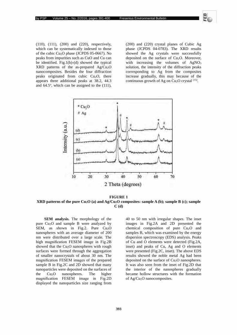
XRD analysis. The XRD patterns of the
prepared pure Cu2O and Ag/Cu2O
nanocomposites sample were shown in Fig.1.
All samples exhibited the same diffraction
peaks at 2θ=29.8, 36.5, 42.6 and 61.4o. These
reflection peaks corresponded to the planes of
by PSP Volume 25 – No. 2/2016, pages 391-400 Fresenius Environmental Bulletin
393
(110), (111), (200) and (220), respectively,
which can be systematically indexed to those
of the cubic Cu2O phase (JCPDS 05-0667). No
peaks from impurities such as CuO and Cu can
be identified. Fig.1(b)-(d) showed the typical
XRD patterns of the as-prepared Ag/Cu2O
nanocomposites. Besides the four diffraction
peaks originated from cubic Cu2O, there
appears three additional peaks at 38.2, 44.3
and 64.5o, which can be assigned to the (111),
(200) and (220) crystal planes of Cubic Ag
phase (JCPDS 04-0783). The XRD results
showed the Ag crystals were successfully
deposited on the surface of Cu2O. Moreover,
with increasing the volumes of AgNO3
solution, the intensity of the diffraction peaks
corresponding to Ag from the composites
increase gradually, this may because of the
continuous growth of Ag on Cu2O crystal [15].
FIGURE 1
XRD patterns of the pure Cu2O (a) and Ag/Cu2O composites: sample A (b); sample B (c); sample
C (d)
SEM analysis. The morphology of the
pure Cu2O and sample B were analyzed by
SEM, as shown in Fig.2. Pure Cu2O
nanospheres with an average diameter of 200
nm were distributed over a large scale. The
high magnification FESEM image in Fig.2B
showed that the Cu2O nanospheres with rough
surfaces were formed through the aggregation
of smaller nanocrystals of about 30 nm. The
magnification FESEM images of the prepared
sample B in Fig.2C and 2D showed that many
nanoparticles were deposited on the surfaces of
the Cu2O nanospheres. The higher
magnification FESEM image in Fig.2D
displayed the nanoparticles size ranging from
40 to 50 nm with irregular shapes. The inset
images in Fig.2A and 2D presented the
chemical composition of pure Cu2O and
samples B, which was examined by the energy
dispersion spectroscopy (EDS) analysis. Peaks
of Cu and O elements were detected (Fig.2A,
inset) and peaks of Cu, Ag and O elements
were presented (Fig.2C, inset). The above EDS
results showed the noble metal Ag had been
deposited on the surface of Cu2O nanospheres.
It was also seen from the inset of Fig.2D that
the interior of the nanospheres gradually
became hollow structures with the formation
of Ag/Cu2O nanocomposites.
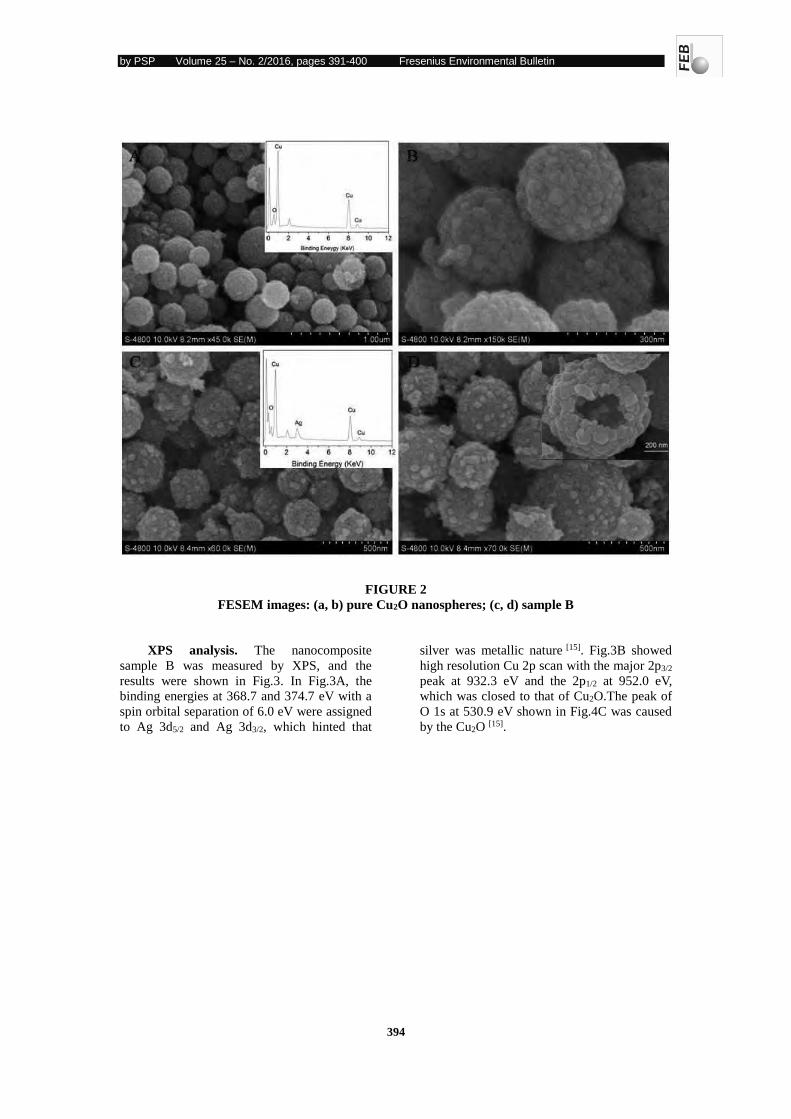
by PSP Volume 25 – No. 2/2016, pages 391-400 Fresenius Environmental Bulletin
394
FIGURE 2
FESEM images: (a, b) pure Cu2O nanospheres; (c, d) sample B
XPS analysis. The nanocomposite
sample B was measured by XPS, and the
results were shown in Fig.3. In Fig.3A, the
binding energies at 368.7 and 374.7 eV with a
spin orbital separation of 6.0 eV were assigned
to Ag 3d5/2 and Ag 3d3/2, which hinted that
silver was metallic nature [15]. Fig.3B showed
high resolution Cu 2p scan with the major 2p3/2
peak at 932.3 eV and the 2p1/2 at 952.0 eV,
which was closed to that of Cu2O.The peak of
O 1s at 530.9 eV shown in Fig.4C was caused
by the Cu2O [15].
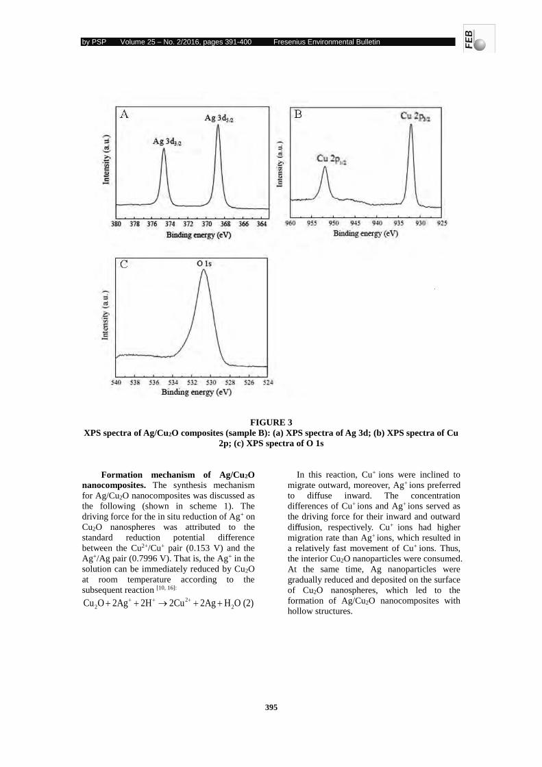
by PSP Volume 25 – No. 2/2016, pages 391-400 Fresenius Environmental Bulletin
395
FIGURE 3
XPS spectra of Ag/Cu2O composites (sample B): (a) XPS spectra of Ag 3d; (b) XPS spectra of Cu
2p; (c) XPS spectra of O 1s
Formation mechanism of Ag/Cu2O
nanocomposites. The synthesis mechanism
for Ag/Cu2O nanocomposites was discussed as
the following (shown in scheme 1). The
driving force for the in situ reduction of Ag+ on
Cu2O nanospheres was attributed to the
standard reduction potential difference
between the Cu2+/Cu+ pair (0.153 V) and the
Ag+/Ag pair (0.7996 V). That is, the Ag+ in the
solution can be immediately reduced by Cu2O
at room temperature according to the
subsequent reaction [10, 16]: 2
2 2Cu O 2Ag 2H 2Cu 2Ag H O (2)
In this reaction, Cu+ ions were inclined to
migrate outward, moreover, Ag+ ions preferred
to diffuse inward. The concentration
differences of Cu+ ions and Ag+ ions served as
the driving force for their inward and outward
diffusion, respectively. Cu+ ions had higher
migration rate than Ag+ ions, which resulted in
a relatively fast movement of Cu+ ions. Thus,
the interior Cu2O nanoparticles were consumed.
At the same time, Ag nanoparticles were
gradually reduced and deposited on the surface
of Cu2O nanospheres, which led to the
formation of Ag/Cu2O nanocomposites with
hollow structures.
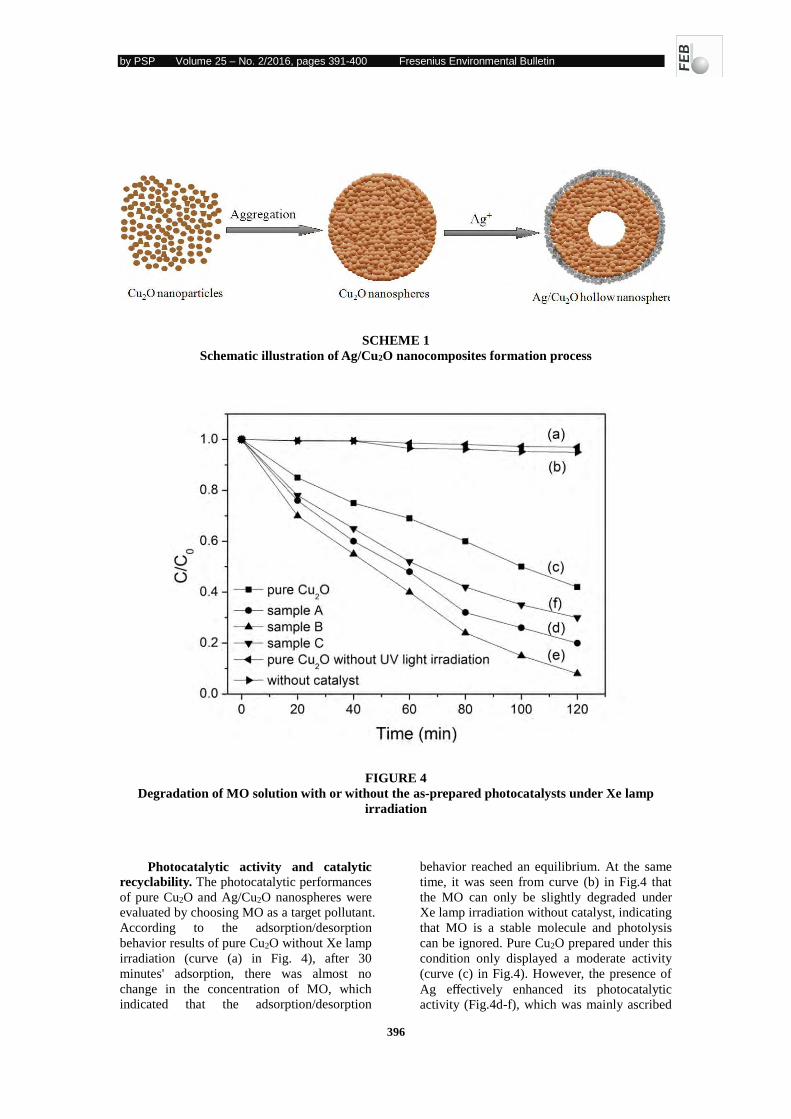
by PSP Volume 25 – No. 2/2016, pages 391-400 Fresenius Environmental Bulletin
396
SCHEME 1
Schematic illustration of Ag/Cu2O nanocomposites formation process
FIGURE 4
Degradation of MO solution with or without the as-prepared photocatalysts under Xe lamp
irradiation
Photocatalytic activity and catalytic
recyclability. The photocatalytic performances
of pure Cu2O and Ag/Cu2O nanospheres were
evaluated by choosing MO as a target pollutant.
According to the adsorption/desorption
behavior results of pure Cu2O without Xe lamp
irradiation (curve (a) in Fig. 4), after 30
minutes' adsorption, there was almost no
change in the concentration of MO, which
indicated that the adsorption/desorption
behavior reached an equilibrium. At the same
time, it was seen from curve (b) in Fig.4 that
the MO can only be slightly degraded under
Xe lamp irradiation without catalyst, indicating
that MO is a stable molecule and photolysis
can be ignored. Pure Cu2O prepared under this
condition only displayed a moderate activity
(curve (c) in Fig.4). However, the presence of
Ag effectively enhanced its photocatalytic
activity (Fig.4d-f), which was mainly ascribed
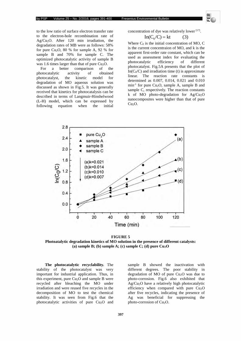
by PSP Volume 25 – No. 2/2016, pages 391-400 Fresenius Environmental Bulletin
397
to the low ratio of surface electron transfer rate
to the electron-hole recombination rate of
Ag/Cu2O. After 120 min irradiation, the
degradation rates of MB were as follows: 58%
for pure Cu2O, 80 % for sample A, 92 % for
sample B and 70% for sample C. The
optimized photocatalytic activity of sample B
was 1.6 times larger than that of pure Cu2O.
For a better comparison of the
photocatalytic activity of obtained
photocatalyst, the kinetic model for
degradation of MO aqueous solution was
discussed as shown in Fig.5. It was generally
received that kinetics for photocatalysis can be
described in terms of Langmuir-Hinshelwood
(L-H) model, which can be expressed by
following equation when the initial
concentration of dye was relatively lower [17].
(3) kt /C)In(C0
Where C0 is the initial concentration of MO, C
is the current concentraion of MO, and k is the
apparent first-order rate constant, which can be
used as assessment index for evaluating the
photocatalytic efficiency of different
photocatalyst. Fig.5A presents that the plot of
In(C0/C) and irradiation time (t) is approximate
linear. The reaction rate constants is
determined as 0.007, 0.014, 0.021 and 0.010
min-1 for pure Cu2O, sample A, sample B and
sample C, respectively. The reaction constants
k of MO photo-degradation for Ag/Cu2O
nanocomposites were higher than that of pure
Cu2O.
FIGURE 5
Photoatalytic degradation kinetics of MO solution in the presence of different catalysts:
(a) sample B; (b) sample A; (c) sample C; (d) pure Cu2O
The photocatalytic recyclability. The
stability of the photocatalyst was very
important for industrial application. Thus, in
this experiment, pure Cu2O and sample B were
recycled after bleaching the MO under
irradiation and were reused five recycles in the
decomposition of MO to test the chemical
stability. It was seen from Fig.6 that the
photocatalytic activities of pure Cu2O and
sample B showed the inactivation with
different degrees. The poor stability in
degradation of MO of pure Cu2O was due to
photo-corrosion. Fig.6 also exhibited that
Ag/Cu2O have a relatively high photocatalytic
efficiency when compared with pure Cu2O
after five recycles, indicating the presence of
Ag was beneficial for suppressing the
photo-corrosion of Cu2O.
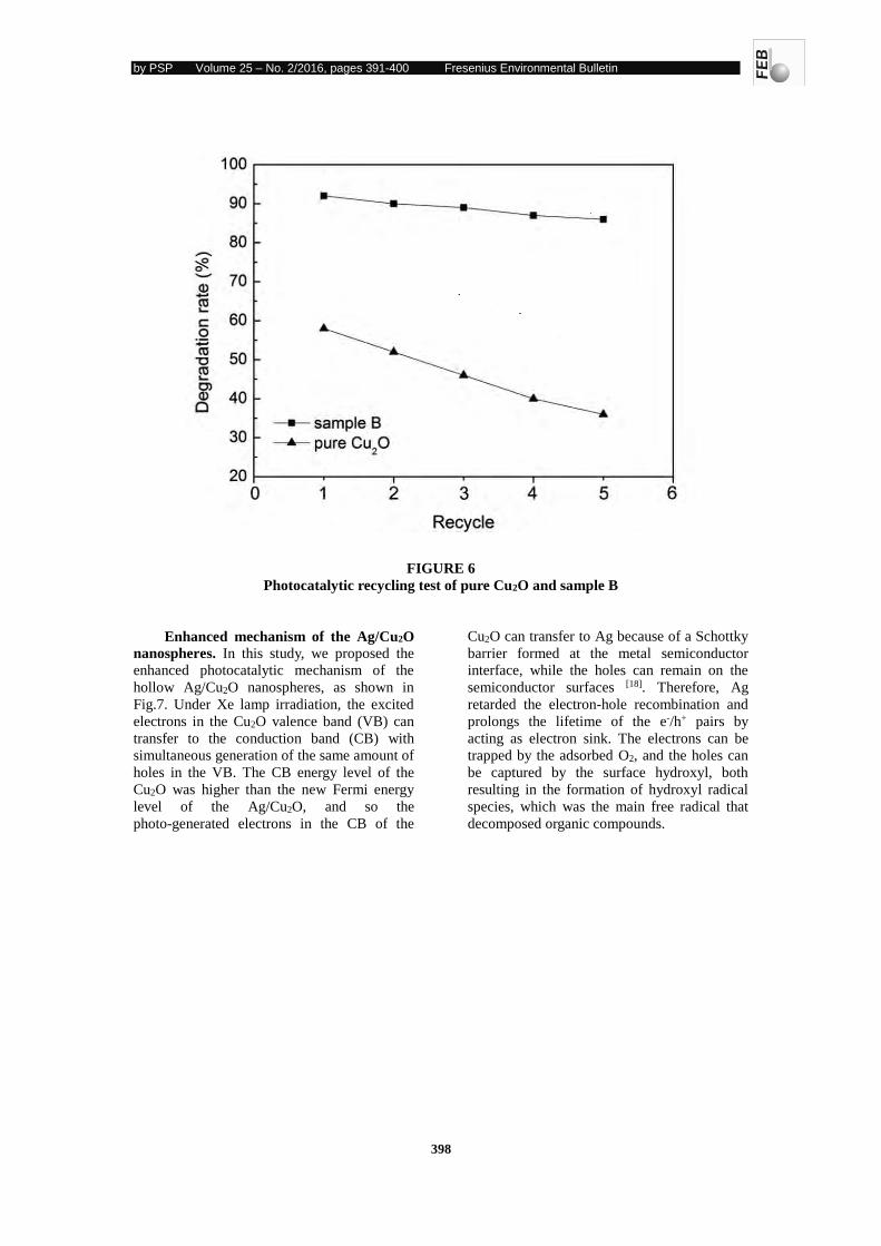
by PSP Volume 25 – No. 2/2016, pages 391-400 Fresenius Environmental Bulletin
398
FIGURE 6
Photocatalytic recycling test of pure Cu2O and sample B
Enhanced mechanism of the Ag/Cu2O
nanospheres. In this study, we proposed the
enhanced photocatalytic mechanism of the
hollow Ag/Cu2O nanospheres, as shown in
Fig.7. Under Xe lamp irradiation, the excited
electrons in the Cu2O valence band (VB) can
transfer to the conduction band (CB) with
simultaneous generation of the same amount of
holes in the VB. The CB energy level of the
Cu2O was higher than the new Fermi energy
level of the Ag/Cu2O, and so the
photo-generated electrons in the CB of the
Cu2O can transfer to Ag because of a Schottky
barrier formed at the metal semiconductor
interface, while the holes can remain on the
semiconductor surfaces [18]. Therefore, Ag
retarded the electron-hole recombination and
prolongs the lifetime of the e-/h+ pairs by
acting as electron sink. The electrons can be
trapped by the adsorbed O2, and the holes can
be captured by the surface hydroxyl, both
resulting in the formation of hydroxyl radical
species, which was the main free radical that
decomposed organic compounds.
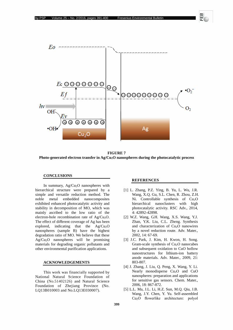
by PSP Volume 25 – No. 2/2016, pages 391-400 Fresenius Environmental Bulletin
399
FIGURE 7
Photo-generated electron transfer in Ag/Cu2O nanospheres during the photocatalytic process
CONCLUSIONS
In summary, Ag/Cu2O nanospheres with
hierarchical structure were prepared by a
simple and versatile reduction method. The
noble metal embedded nanocomposites
exhibited enhanced photocatalytic activity and
stability in decomposition of MO, which was
mainly ascribed to the low ratio of the
electron-hole recombination rate of Ag/Cu2O.
The effect of different coverage of Ag has been
explored, indicating that the Ag/Cu2O
nanospheres (sample B) have the highest
degradation ratio of MO. We believe that these
Ag/Cu2O nanospheres will be promising
materials for degrading organic pollutants and
other environmental purification applications.
ACKNOWLEDGEMENTS
This work was financially supported by
National Natural Science Foundation of
China (No.51402126) and Natural Science
Foundation of Zhejiang Province (No.
LQ13B010003 and No.LQ13E030007).
REFERENCES
[1] L. Zhang, P.Z. Ying, B. Yu, L. Wu, J.R.
Wang, X.Q. Gu, S.L. Chen, R. Zhou, Z.H.
Ni. Controllable synthesis of Cu2O
hierarchical nanoclusters with high
photocatalytic activity. RSC Adv., 2014,
4: 42892-42898.
[2] W.Z. Wang, G.H. Wang, X.S. Wang, Y.J.
Zhan, Y.K. Liu, C.L. Zheng. Synthesis
and characterization of Cu2O nanowires
by a novel reduction route. Adv. Mater.,
2002, 14: 67-69.
[3] J.C. Park, J. Kim, H. Kwon, H. Song.
Gram-scale synthesis of Cu2O nanocubes
and subsequent oxidation to CuO hollow
nanostructures for lithium-ion battery
anode materials. Adv. Mater., 2009, 21:
803-807.
[4] J. Zhang, J. Liu, Q. Peng, X. Wang, Y. Li.
Nearly monodisperse Cu2O and CuO
nanospheres: preparation and applications
for sensitive gas sensors. Chem. Mater.,
2006, 18: 867-872.
[5] L.L. Ma, J.L. Li, H.Z. Sun, M.Q. Qiu, J.B.
Wang, J.Y. Chen, Y. Yu. Self-assembled
Cu2O flowerlike architecture: polyol
by PSP Volume 25 – No. 2/2016, pages 391-400 Fresenius Environmental Bulletin
400
synthesis, photocatalytic activity and
stability under simulated solar light.
Mater. Res. Bull., 2010, 45: 961-968.
[6] R. Georgekutty, M.K. Seery, S.C. Pillai. A
highly efficient Ag-ZnO photocatalyst:
synthesis, properties, and mechanism. J.
Phys. Chem. C, 2008, 112: 13563-13570.
[7] W. Lu, S. Gao, J. Wang. One-pot synthesis
of Ag/ZnO self-assembled 3D hollow
microspheres with enhanced
photocatalytic performance. J. Chem.
Phys. C, 2008, 112: 16792-16800.
[8] W. Jia, B. Jia, F. Qu. Towards a highly
efficient simulated sunlight driven photocatalyst: a case of heterostructured
ZnO/ZnS hybrid structure. Dalton Trans.,
2013, 42: 14178-14187.
[9] J. Wang, F. Qu, X. Wu. Photocatalytic
degradation of organic dyes with
hierarchical Ag2O/ZnO heterostructures.
Sci. Adv. Mater., 2013, 5: 1364-1371.
[10] W.X, Zhang, X.N. Yang, Q. Zhu, K. Wang,
J.B. Lu, M. Chen, Z.H. Yang. One-Pot
Room Temperature Synthesis of
Cu2O/Ag Composite Nanospheres with
Enhanced Visible-Light-Driven
Photocatalytic Performance. Industrial &
Engineering Chemistry Research, 2014,
53: 16316-16323.
[11] D.D. Lin, H. Wu, R. Zhang and W. Pan.
Enhanced photocatalysis of electrospun
Ag-ZnO heterostructured nanofibers.
Chem. Mater., 2009, 21: 3479-3484.
[12] P. Li, Z. Wei, T. Wu, Q. Peng, Y.D. Li.
Au-ZnO Hybrid Nanopyramids and Their
Photocatalytic Properties. J. Am. Chem.
Soc., 2011, 133: 5660-5663.
[13] H.B. Zeng, W.P. Cai, P.S. Liu, X.X. Xu, H.
J. Zhou,C. Klingshirn, H. Kalt.
ZnO-Based Hollow Nanoparticles by
Selective Etching: Elimination and
Reconstruction of Metal Semiconductor
Interface, Improvement of Blue Emission
and Photocatalysis. ACS Nano, 2008, 2:
1661-1670.
[14] H. B. Zeng, P. S. Liu, W. P. Cai, S. K.
Yang and X. X. Xu. Controllable Pt/ZnO
Porous Nanocages with Improved
Photocatalytic Activity. J.Phys. Chem. C,
2008, 112: 19620-19624.
[15] J.B. Yang, Z. Li, C.X. Zhao, Y. Wang,
X.Q. Liu. Facile synthesis of Ag-Cu2O
composites with enhanced photocatalytic
activity. Mater. Res. Bull., 2014, 60:
530-536.
[16] J. Wang, F.L. Cui, S.B. Chu, X.Q. Jin, J.
Pu, Z.H. Wang. In situ Growth of
Noble-Metal Nanoparticles on Cu2O
Nanocubes for Surface-Enhanced Raman
Scattering Detection.
CHEMPLUSCHEM, 2014, 79: 684-689.
[17] R.G. Chen, J.H. Bi, L. Wu, Z.H. Li, X.Z.
Fu. Orthorhombic Bi2GeO5 nanobelts:
Synthesis, characterization, and
photocatalytic properties. Cryst. Growth
Des., 2009, 9: 1775-1779.
[18] Y.G. Chang, J. Xu, Y.Y. Zhang, S.Y. Ma,
L.H. Xin, L.N. Zhu, C.T. Xu. Optical
Properties and Photocatalytic
Performances of Pd Modified ZnO Samples. J. Phys. Chem. C, 2009, 113:
18761-18767.
Received: 09.06.2015
Accepted: 16.06.2015
CORRESPONDING AUTHOR
Hongmei Wang
Institute of Biological and Chemical
Engineering
Jiaxing University
Jiaxing 314001 - P.R. China
e-mail: [email protected]
by PSP Volume 25 – No. 2/2016, pages 401-408 Fresenius Environmental Bulletin
401
DETERMINATION OF LEAD, MERCURY, ARSENIC AND
CADMIUM LEVEL IN MUSCLE OF COMMON CARP
(CYPRINUS CARPIO) IN SOUTHERN CASPIAN SEA AND
GOMISHAN AND ANZALI WETLANDS
Mohammad Reza Ghomi
Department of Fisheries, Tonekabon Branch, Islamic Azad University, Tonekabon, Iran
ABSTRACT
Due to the importance of Caspian Sea as the
largest brakish water body in the world, the present
study has been done to assess the level of common
carp (Cyrprinus carpio) muscle contamination in
the five regions of southern Caspian Sea for the
main hazardous heavy metals. The mean level of all
measured heavy metals (Pb= 0.192, Cd= 0.111,
Hg= 0.027, As= 0.014 μg/g wet weight), in the five different sites of the southern Caspian Sea
(including Anzali and Gomishan wetlands) were
below than standard. Western sampling site of the
southeast Caspian Sea, had the trend of maximum
levels of metals comparing to the other sampling
sites, and then followed by the eastern sampling
area and Gomishan wetland. The middle sampling
site of the southern Caspian Sea showed the
minimum of all heavy metals in present study
indicating the pollution of this area is lower than
other sampling regions. By having the deepest
water in the middle of southern Caspian Sea (the
average depth of 342 m) and water circulations that
mainly occurring time to time there, more water
movement in this area could be expected that could
potentially incorporated the benefit of more dilution
of contamination and resulting the minimum level
of all measured metals in carp muscle in this area
rather than other western and eastern basins.
KEYWORDS: Heavy metals, Caspian Sea, Gomishan wetland, Anzali
wetland, Common carp
INTRODUCTION
Since industrialization in the late 1940s and
1950s, the amount of contaminants and toxic
substances put into the oceans has greatly increased [1]. These contaminants include heavy metals such
as Hg, Pb, Cd, Zn, Cr and Cu and synthetic organic
compounds [1]. The main sources of heavy metals
are the erosion of soils, rocks and also from the
industrial and urban wastes are discharged into
water bodies [2]. Also, sub marine volcanic activities
and leaching of the ocean floor are also among the
natural processes that have caused the enrichments
of these elements [3]. These elements have no
beneficial effects in humans, and there is no known
homeostasis mechanism for them [4]. Although
toxicity and the resulting threat to human health of
any contaminant are, of course, a function of
concentration, it is well-known that chronic
exposure to As, Cd, Hg, and Pb at relatively low
levels can cause adverse effects [5].
According to USEPA [6], the human activities
is one of the main origin of all mentioned heavy
metals in which arsenic compounds, mainly As2O3,
can be recovered as a by-product of processing
complex ores mined mainly for copper, Pb, zinc,
gold, and silver. Pure cadmium compounds rarely
are found in nature, although the main sources of
Cd are sulfide ores of Pb, zinc, and copper.
Recovery of lead from the ore typically involves
grinding, flotation, roasting, and smelting. And in a
few cases, mercury occurs as the principal ore
product; it is more commonly obtained as the
byproduct of processing complex ores that contain
mixed sulfides, oxides, and chloride minerals [6].
The Caspian Sea by constituting 44% of the
global volume of lacustrine waters is the largest
enclosed water body on the earth [7]. The Caspian
Sea has an elongated geometry (1000 km in length
and 200–300 km in width), where the Northern,
Middle and Southern Caspian Basins that has
maximum depth of about 20 m, 788 m and 1025 m,
respectively [7]. The Caspian Sea and related water
including Gomishan and Anzali wetlands have the
particular circumstances of species diversity of
plants and animals. The wetlands in the southern
part of the Caspian Sea in the North Iran are
seriously threatened by pollutants from various
sources influenced by industrial, shipping,
agriculture, Caspian oil.
The Anzali wetland is situated at the
southwest of the Caspian Sea (37˚ 28/N, 49˚ 25/E). The Anzali wetland's area is more than 218 km2
by PSP Volume 25 – No. 2/2016, pages 401-408 Fresenius Environmental Bulletin
402
which consists of the total basin of 374,000 hectare
with the maximum depth of 3.5 m and average
depth of more than 1 m. According to Ramsar
Convention in 1975, among the twenty preserved
wetlands in Iran, this wetland is considered as one
of the most important wetlands. The wetland is
currently receiving mass and energy flows of the
eleven midsize catchments and their rivers
originating from the northern mountains with
relatively steep slopes toward the wetland [8].
The Gomishan wetland is situated at the
southeast of the Caspian Sea (37˚ 11/N, 53˚ 57/E). It is a type of large shallow marsh lagoon with a
surface area of 20,000 ha, average depth of 1 m,
and maximum depth of 2.5 m [9]. Research on
physicochemical characteristics of international
Gomishan wetland showed that increasing
agricultural activities and application of chemical
pesticides, wastes, municipal and industrial
wastewater seriously imposed the risks to the
aquatic ecosystems [10].
Sea food has an important role in human
nutrition which brings health for human
consumption. According to IFO [11], the stocking of
common carp fingerling in Caspian Sea was
reached to 340,000 individuals in 2005. Farmed
common carp production was nearly 14 percent of
the total global freshwater aquaculture production
in 2002 (33,138,962 tonnes) which indicates high
demand of this species for human consumption.
Common carp production increased by an average
global rate of 9.5 percent/year between 1985 and
2002 [12].
Compared to other semi-enclosed and
enclosed seas of the world, little is known of the
Caspian Sea contamination especially in its
consumable fish metals. Present study was aimed to
measure the four heavy metals (Cd, As, Pb, Hg) in
muscle of common carp (Cyrprinus carpio) caught
from southern Caspian Sea and Anzali and
Gomishan wetlands to monitor their levels in
different areas and also comparing with the
international standards.
MATERIALS AND METHODS
Five common carp (Cyrprinus carpio) samples
in the five different stations (sampling sites no. 1-5)
of the southern Caspian Sea including Gomishan
wetland (no. 1), south-eastern Caspian Sea (no. 2),
south-middle Caspian Sea (no. 3), Anzali wetland
(no. 4), and the south-western Caspian Sea (no. 5)
randomly caught (totally 25 samples) (Figure 1).
The samples were in the weight range of 870 ± 83
g. Samples after being placed in a flask containing
ice, immediately transported to the laboratory.
In the laboratory, the samples were washed
with distilled water, then skin was separated from
the muscle and muscle was kept to measure metals.
Then 10 g of the muscle tissue samples were
removed to be ready for conduction of chemical
digestion [13]. Ten gram of sample is poured into a
Pyrex flask and for digestion of heavy metals, a
combination of 50 ml pure nitric acid with 50 ml of
30% hydrogen peroxide was added in. Then the
samples exposed to the temperature ranging 100-
150 °C and acid digestion occurred. The digestion
process took for 30-60 min to reach to 5 ml of the
initial solution, 5 ml deionized water added to reach
to a volume of 10 ml (with deionized water) and
finally was filled in 20 ml glass containers for
measurement of heavy metals [13]. In order to avoid
probable contamination, all the glassware and
equipment used were washed by 4% Nitric acid.
The four heavy metals including lead, mercury,
arsenic and cadmium were measured by standard
method using atomic absorption spectroscopy
(Varian AA-240FS, USA) in ppb. The data were
reported as μg/g wet weight (ww) of fish muscle. The test of kolmogrov-Smirnov for
determination of normality of data distribution was
examined, and based on normality of data, the
differences between groups were compared using
one-way ANOVA and Duncan's multiple range test
in the level of 95%. Statistical analysis was
performed using SPSS16 software.
Statistical software, version 5.1 (SAS Institute
INc., Cary, NC, USA). Sources of variation were
treatments, incubation day and their interaction.
Means were compared by Student’s t-test at a
significance level of 0.01 or 0.05.
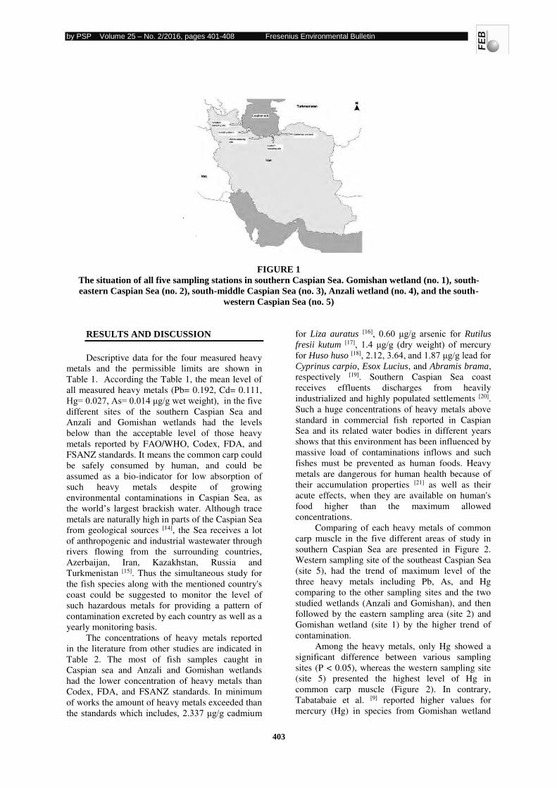
by PSP Volume 25 – No. 2/2016, pages 401-408 Fresenius Environmental Bulletin
403
FIGURE 1
The situation of all five sampling stations in southern Caspian Sea. Gomishan wetland (no. 1), south-
eastern Caspian Sea (no. 2), south-middle Caspian Sea (no. 3), Anzali wetland (no. 4), and the south-
western Caspian Sea (no. 5)
RESULTS AND DISCUSSION
Descriptive data for the four measured heavy
metals and the permissible limits are shown in
Table 1. According the Table 1, the mean level of
all measured heavy metals (Pb= 0.192, Cd= 0.111,
Hg= 0.027, As= 0.014 μg/g wet weight), in the five different sites of the southern Caspian Sea and
Anzali and Gomishan wetlands had the levels
below than the acceptable level of those heavy
metals reported by FAO/WHO, Codex, FDA, and
FSANZ standards. It means the common carp could
be safely consumed by human, and could be
assumed as a bio-indicator for low absorption of
such heavy metals despite of growing
environmental contaminations in Caspian Sea, as
the world’s largest brackish water. Although trace metals are naturally high in parts of the Caspian Sea
from geological sources [14], the Sea receives a lot
of anthropogenic and industrial wastewater through
rivers flowing from the surrounding countries,
Azerbaijan, Iran, Kazakhstan, Russia and
Turkmenistan [15]. Thus the simultaneous study for
the fish species along with the mentioned country's
coast could be suggested to monitor the level of
such hazardous metals for providing a pattern of
contamination excreted by each country as well as a
yearly monitoring basis.
The concentrations of heavy metals reported
in the literature from other studies are indicated in
Table 2. The most of fish samples caught in
Caspian sea and Anzali and Gomishan wetlands
had the lower concentration of heavy metals than
Codex, FDA, and FSANZ standards. In minimum
of works the amount of heavy metals exceeded than
the standards which includes, 2.337 μg/g cadmium
for Liza auratus [16], 0.60 μg/g arsenic for Rutilus
fresii kutum [17], 1.4 μg/g (dry weight) of mercury for Huso huso [18], 2.12, 3.64, and 1.87 μg/g lead for Cyprinus carpio, Esox Lucius, and Abramis brama,
respectively [19]. Southern Caspian Sea coast
receives effluents discharges from heavily
industrialized and highly populated settlements [20].
Such a huge concentrations of heavy metals above
standard in commercial fish reported in Caspian
Sea and its related water bodies in different years
shows that this environment has been influenced by
massive load of contaminations inflows and such
fishes must be prevented as human foods. Heavy
metals are dangerous for human health because of
their accumulation properties [21] as well as their
acute effects, when they are available on human's
food higher than the maximum allowed
concentrations.
Comparing of each heavy metals of common
carp muscle in the five different areas of study in
southern Caspian Sea are presented in Figure 2.
Western sampling site of the southeast Caspian Sea
(site 5), had the trend of maximum level of the
three heavy metals including Pb, As, and Hg
comparing to the other sampling sites and the two
studied wetlands (Anzali and Gomishan), and then
followed by the eastern sampling area (site 2) and
Gomishan wetland (site 1) by the higher trend of
contamination.
Among the heavy metals, only Hg showed a
significant difference between various sampling
sites (P < 0.05), whereas the western sampling site
(site 5) presented the highest level of Hg in
common carp muscle (Figure 2). In contrary,
Tabatabaie et al. [9] reported higher values for
mercury (Hg) in species from Gomishan wetland
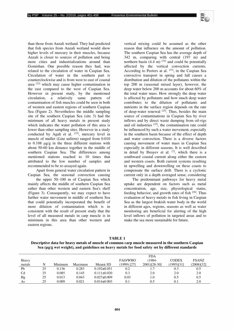
by PSP Volume 25 – No. 2/2016, pages 401-408 Fresenius Environmental Bulletin
404
than those from Anzali wetland. They had predicted
that fish species from Anzali wetland would show
higher levels of mercury in their muscles, because
Anzali is closer to sources of pollution and being
more cities and industrializations around than
Gomishan. One possible reason they had, was
related to the circulation of water in Caspian Sea.
Circulation of water in the southern part is
counterclockwise and is from west to east of coastal
area [22] which may cause higher contamination in
the east compared to the west of Caspian Sea.
However in present study, by the mentioned
circulation, a relatively same pattern of
contamination of fish muscles could be seen in both
of western and eastern regions of southern Caspian
Sea (Figure 2). Nevertheless the middle sampling
site of the southern Caspian Sea (site 3) had the
minimum of all heavy metals in present study
which indicates the water pollution of this area is
lower than other sampling sites. However in a study
conducted by Agah et al. [23], mercury level in
muscle of mullet (Liza saliens) ranged from 0.010
to 0.108 μg/g in the three different stations with
about 50-60 km distance together in the middle of
southern Caspian Sea. The differences among
mentioned stations reached to 10 times that
attributed to the low number of samples and
recommended to be re-assayed again.
Apart from general water circulation pattern in
Caspian Sea, the seasonal convection causing
vertical mixing could be assumed as the other
reason that influence on the amount of pollution.
The southern Caspian Sea has the average depth of
342 m, comparing with central (197 m) and
northern basin (4.4 m) [24] and could be potentially
affected by the vertical convection currents.
According to Peeters at al. [25], in the Caspian Sea
convective transport in spring and fall causes a
distribution and dilution of the pollutants within the
top 200 m (seasonal mixed layer), however, the
deep water below 200 m accounts for about 60% of
the total water mass. How strongly the deep water
is affected by pollutants and how much deep water
contributes to the dilution of pollutants and
nutrients in the surface region depends on the rate
of deep-water renewal [25]. Thus, besides the main
source of contaminations in Caspian Sea by river
inflows and by direct waste dumping from oil-rigs
and oil industries [25], the contamination rate could
be influenced by such a water movement, especially
in the southern basin because of the effect of depth
and water convection. There is a diverse factors
causing movement of water mass in Caspian Sea
especially in different seasons. It is well described
in detail by Ibrayev et al. [7], which there is a
southward coastal current along either the eastern
and western coasts. Both current systems resulting
in upwelling and downwelling on these coasts to
compensate the surface drift. There is a cyclonic
current only in a depth averaged sense, considering
the upper 50–100 m of Caspian Sea which
mainly affects the middle of southern Caspian Sea
rather than other western and eastern Sea's shelf
(Figure 3). Consequently, we may expect to have
further water movement in middle of southern Sea
that could potentially incorporated the benefit of
more dilution of contamination which is in
consistent with the result of present study that the
level of all measured metals in carp muscle is in
minimum in this area than other western and
eastern regions.
The predominant pathways for heavy metal
uptake are dependent on factors such as metal
concentration, age, size, physiological status,
feeding behavior, and growth rates of fish [26]. Thus
evaluation of heavy metals in fish living in Caspian
Sea as the largest brakish water body in the world
in different ages, regions, seasons as well as water
monitoring are beneficial for alerting of the high
level inflows of pollution in targeted areas and to
make the sea more sustainable for future.
TABLE 1
Descriptive data for heavy metals of muscle of common carp muscle measured in the southern Caspian
Sea (μg/g wet weight), and guidelines on heavy metals for food safety set by different standards
Heavy
metals N Minimum Maximum Mean± SD
FAO/WHO
(1999) [27]
FDA
(1984-
2001)[28-30]
CODEX
(1995)[31]
FSANZ
(2008)[32]
Pb 25 0.136 0.283 0.192±0.051 0.2 1.7 0.3 0.5
Cd 25 0.085 0.145 0.111±0.020 0.3 2.0 2.0 2.0
Hg 25 0.013 0.043 0.027±0.009 0.03 1.0 0.5 0.5
As 25 0.009 0.021 0.014±0.003 0.1 0.5 0.1 2.0
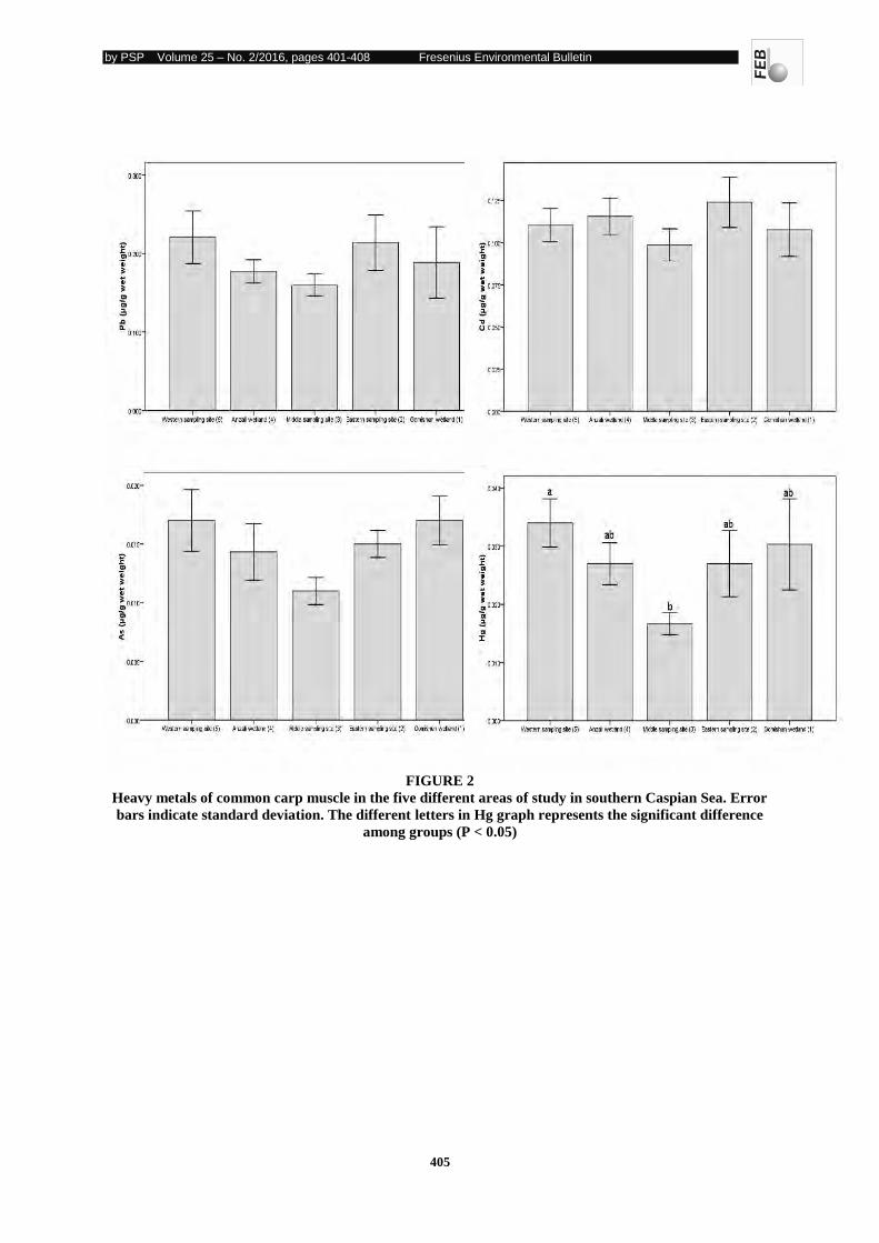
by PSP Volume 25 – No. 2/2016, pages 401-408 Fresenius Environmental Bulletin
405
FIGURE 2
Heavy metals of common carp muscle in the five different areas of study in southern Caspian Sea. Error
bars indicate standard deviation. The different letters in Hg graph represents the significant difference
among groups (P < 0.05)
by PSP Volume 25 – No. 2/2016, pages 401-408 Fresenius Environmental Bulletin
406
TABLE 2
Heavy metal levels in various fish species in the Caspian Sea (μg/g wet weight) Species
Water body Cd As Hg Pb Reference
Rutilus rutilus caspicus Caspian sea 0.04 - - 0.04 Taghipour and Azizi,
2011
Liza auratus Caspian sea 2.337 - - 0.321 Pourang et al. 2005
Cyprinus carpio Gomishan wetland 0.03 - - 0.07 Bandani et al. 2010
Cyprinus carpio Caspian sea 0.01 - 0.13 - Saravi et al. 2013
Rutilus fresii kutum Eastern Caspian sea 0.004 - 0.001 0.012 Varedi (2006)
Liza saliens Eastern Caspian sea 0.631 - 0.001 2.63 Varedi (2006)
Rutilus fresii kutum Caspian sea 0.001 - 0.19 0.008 Anan et al. 2005
Huso huso Caspian sea - - 1.4 (dry weight) - Agusa et al. (2004)
Acipenser persicus Caspian sea - - 0.33 (dry
weight)
- Agusa et al. (2004)
Acipenser stellatus Caspian sea - - 0.06 (dry
weight)
- Agusa et al. (2004)
Rutilus fresii kutum Middle Caspian sea 0.004 0.60 0.13 0.042 Agah et al. 2010
Liza aurata Middle Caspian sea 0.005 0.31 0.07 0.032 Agah et al. 2010
Different species Middle Caspian sea 0.005 0.40 0.021 - Agah et al. 2007
Carassius gibelio Anzali wetland 0.21 - - 0.90 Ebrahimpour et al. 2011
Cyprinus carpio Anzali wetland 0.23 - - 2.12 Mansouri et al. 2013
Esox lucius Anzali wetland 0.31 - - 3.64 Mansouri et al. 2013
Abramis brama Anzali wetland 0.24 - - 1.87 Mansouri et al. 2013
Cyprinus carpio Anzali and Gomishan
wetland
- - 0.2 - Tabatabaie et al. 2011
Sander lucioperca Anzali wetland - - 0.06 - Tabatabaie et al. 2011
Sander lucioperca Gomishan wetland - - 0.15 - Tabatabaie et al. 2011
Cyprinus carpio Caspian sea, Anzali and
Gomishan wetland
0.111 0.014 0.027 0.192 Present study
FIGURE 3
Monthly currents at 50 m depth of Caspian Sea (Ibrayev et al., [7]). The current is mainly affected the
middle of southern basin rather than eastern and western shelf
ACKNOWLEDGMENTS
This study has been supported as a research
project (N0. 37689) of Islamic Azad University,
Tonekabon branch, Iran.
REFERENCES
[1] USEPA (United States Environmental
Protection Agency) (2006) Contaminants and
toxic chemicals, heavy metals, pesticides,
PCBs, and PAHs. Washington, D.C.
[2] Yu KY, Tasi LJ, Chen SH, Ho ST (2001)
Chemical binding of heavy metals in anoxic
river sediments. Water Resour 35(7):4086–4094.
[3] Hashim NO (2001) The levels of
radionuclides and trace elements in selected
Kenyan coastal ecosystems. A thesis
submitted in partial fulfillment for the
requirement of the degree of Masters of
Science in Physics of Kenyatta University.
by PSP Volume 25 – No. 2/2016, pages 401-408 Fresenius Environmental Bulletin
407
[4] Chang LW (1996) Toxicology of Metals;
CRC Lewis Publishers: Boca Raton, FL, USA.
[5] Llobet JM, Falcoä G, Casas C, Teixidoä A,
Domingo JL (2003) Concentrations of arsenic,
cadmium, mercury, and lead in common foods
and estimated daily intake by children,
adolescents, adults, and seniors of Catalonia,
Spain. J Agric Food Chem 51:838-842.
[6] USEPA (United States Environmental
Protection Agency) (1997) Technology
alternatives for the remediation of soils
contaminated with As, Cd, Cr, Hg, and Pb.
Office of Emergency and Remedial Response.
Washington, D.C.
[7] Ibrayev RA, Ozsoy E, Schrum C, Sur HI
(2010) Seasonal variability of the Caspian Sea
three-dimensional circulation, sea level and
air-sea interaction. Ocean Sci 6:311–329.
[8] Kazanci N, Gulbabazadeh T, Leroy SAG, Ileri
O (2004) Sedimentary and environmental
characteristics of the Gilan-Mazenderan plain,
northern Iran: influence of long- and short-
term Caspian water level fluctuations on
geomorphology. J Marine Sys 46(1-4):145-
168.
[9] Tabatabaie T, Ghomi MR, Amiri F, Zamani-
ahmadmahmoodi R (2011) Comparative study
of mercury accumulation in two fish species,
(Cyprinus carpio and Sander lucioperca) from
Anzali and Gomishan wetlands in the southern
coast of the Caspian Sea, Bull Environ
Contam Toxicol 87(6):674-677.
[10] Kiabi b, Vertical B, Abdul A (1999)
Ecosystems in wetlands and rivers in Golestan
province, Volume I. Published by the
Environmental Protection Agency. 174 P. (In
Farsi)
[11] IFO (Iranian Fisheries Organization) (2005) A
decade activities of Iranian Fisheries
Organization (1993-2005). (In Farsi)
[12] FAO (2014) Cultured aquatic species
information program, Cyprinus
carpio (Linnaeus, 1758).
http://www.fao.org/fishery/culturedspecies/Cy
prinus_carpio/en.
[13] Voegborlo RB, Adimado AA, Ephraim JH
(2007) Total mercury distribution in different
tissues of frigate tuna (Auxis thazard thazard)
from the Atlantic coastal waters of Ghana,
Gulf of Guinea. Environ Mon Assess
132:503–508. [14] CEP (2006) Caspian Environmental Program,
http://www.caspianenvironment. org/ caspian.
Htm.
[15] Katunin DN (2000) Ecological and
toxicological characteristics of Volga. Caspian
basin in the conditions of anthropogenic
impact on biological resources and habitat.
Fishery studies in the Caspian- Results of
scientific research works over 1999-
Astrakhan. Caspian Scientific Research
Institute of Fishery. Pages 30-44.
[16] Pourang N, Tanabe S, Rezvani S, Dennis JH
(2004) Trace elements accumulation in edible
tissues of five sturgeon species from the
Caspian Sea. Environ Monit Assess 100(1-
3):89-108.
[17] Agah H, Eghtesadi P, Owfi F, Fatemi SMR
(2010) Concentrations of some trace metals in
the tissues of two commercial fishes from
Tonekabon. J Persian Gulf (Mar Sci) 1(2):55-
64.
[18] Agusa T, Kunito T, Tanabe S, Pourkazemi M,
Aubery DG (2004) Concentration of trace
elements in muscle of sturgeons in the
Caspian Sea. Mar Pollut Bull 49:789–800.
[19] Mansouri N, Khorasani N, Karbassi AR, Riazi
B, Panahandeh M (2013) Assesing human risk
of contaminants in Anzali wetland fishes. Int J
Appl Innov Eng Manag 2( 11):119-126.
[20] Tabari S, Saravi SS, Bandany GA, Dehghan
A, Shokrzadeh M (2010) Heavy metals (Zn,
Pb, Cd and Cr) in fish, water and sediments
sampled form Southern Caspian Sea, Iran.
Toxicol Ind Health 26(10):649-656.
[21] Tressou J, Crepet A, Bertall P, Feinberg MH,
Leblanc JC (2004) Probabilistic exposure
assessment to food chemicals based on
extreme value theory, application to heavy
metals from fish and sea products. Food Chem
Toxicol 42:1349.
[22] Korotenko KA, Mamedove RM, Mooers CNK
(2000) Prediction of the dispersal of oil
transport in the Caspian Sea resulting from a
continuous release. Spill Sci Technol Bull 6(5-
6):323-339.
[23] Agah H, Leermakers M, Elskens M, Fatemi
SMR, Baeyens W (2007) Total mercury and
methyl mercury concentrations in fish from
the Persian gulf and the Caspian Sea. Water
Air Soil Pollut DOI 10.1007/s11270-006-
9281-0.
[24] Kosarev AN, Yablonskaya EA (1994) The
Caspian Sea, SPB Academic Publishing. The
Hague, 259 pp.
[25] Peeters F, Kipfer R, Achermann D, Hofer M,
Aeschbach-Hertig W, Beyerle U, Imboden
DM, Rozanski K, Frohlich K (2000) Analysis
of deep-water exchange in the Caspian Sea
based on environmental tracers. Deep Sea Res,
Part I 47:621–654.
[26] Chapman PM, Allen HE, Godtfredsen K,
Z'graggen MN (1996) Evaluation of
by PSP Volume 25 – No. 2/2016, pages 401-408 Fresenius Environmental Bulletin
408
bioaccumulation factors in regulating metals.
Environ Sci Technol 30:448-452.
[27] FAO/WHO (1999) Expert Committee on Food
Additives, Summary and conclusions, 53rd
Meeting, Rome.
[28] FDA (US Food and Drug Administration)
(1984) Action level for methyl mercury in
fish, Federal Register 49, Nov. 19, 45663.
[29] FDA (U.S. Food and Drug Administration)
(1999) U.S. Department of health and human
Services, 21 CFR 556.60.
[30] FDA (U.S. Food and Drug Administration)
(2001) Fish and fisheries products hazards and
controls guidance, 3rd edn., Center for Food
Safety and Applied Nutrition, US Food and
Drug Administration.
[31] CODEX (1995) Codex general standard for
contaminants and toxins in food and feed.
CODEX STAN 193.
[32] FSANZ (Food Standards Australia New
Zealand) (2008) Code – Amendment No. 97.
Anstat Pty Ltd., Melbourne.
[33] Ebrahimpour M, Pourkhabbaz A, Baramaki
R, Babaei H, Rezaei M (2011)
Bioaccumulation of heavy metals in
freshwater fish species, Anzali, Iran. Bull
Environ Contam Toxicol. 87(4):386-392.
Received: 09.06.2015 Accepted: 05.12.2015
CORRESPONDING AUTHOR
Mohammad Reza Ghomi
Department of Fisheries
Tonekabon Branch
Islamic Azad University
Tonekabon – IRAN
e-mail: [email protected]
by PSP Volume 25 – No. 2/2016, pages 409-418 Fresenius Environmental Bulletin
409
RENEWABLE ENERGY STATUS AND HYDROPOWER IN
SOME DEVELOPING COUNTRIES AND FOCUS ON TURKEY
Ibrahim Yuksel1; Hasan Arman2; Ugur Serencam3 Mehmet Songur4; I. Halil Demirel5
1 Yildiz Technical University, Civil Engineering Faculty, Department of Civil Engineering, Hydraulics Division, 34220 Davutpasa-Istanbul, Turkey
2 United Arab Emirates University, College of Science, Geology Department, 15551, Al-Ain, UAE 3 Bayburt University, Engineering Faculty, Dep. of Civil Engineering, 68000 Bayburt, Turkey
4 Sakarya University, Civil Engineering Ph.D. Student, 54187, Sakarya, Turkey 5 Yildiz Technical University, Civil Engineering Ph.D. Student, 34220, Istanbul, Turkey
ABSTRACT
The share of renewable energies varies quite a lot
in the developing countries, both in terms of total
primary energy and electricity generation. Several
different policy instruments are in use for promoting
renewable energies, such as quota obligations, price
subsidies, and taxes/tax exemptions on energy. Some
countries such as Turkey, also have specific political
programs for renewable energies. The obstacles and
success conditions mainly deal with geographical,
economic, administrative and political factors. The
Republic of Turkey forms a natural bridge between
Europe and Asia and the country has a relatively
young population in both Europe and Asia. Turkey
aims to utilize its energy potential, including from
renewable sources, in a cost-effective manner. In its
efforts to promote renewable energy, the government
has focused on electricity, but has recently started to
pay more attention to heat. On the other hand,
Turkey’s geographical location has several advantages for extensive use of most of the renewable energy
sources. In this regard, renewable energy resources
appear the most efficient and effective solutions for
clean and sustainable energy development in Turkey.
In addition to Turkey has a great hydropower,
especially small hydropower potential. This paper
deals with Turkey’s renewable energy status in
developing countries.
KEYWORDS: Renewable energy; hydropower; developing counties;
Turkey
INTRODUCTION
In September 2001, the European Parliament and
the Council gave the Directive 2001/77/EC (EC,
2001) on the promotion of electricity produced from
renewable energy sources in the internal electricity
market. The background for this directive includes the
underused potential of exploitation of renewable
energy and the need to promote renewable energies as
a priority measure to contribute to environmental
protection and sustainable development. In addition,
renewable energies offer a possibility to increase local
employment, social cohesion and security of energy
supply as well as they help in meeting the European
Union (EU) target in the Kyoto Protocol of the United
Nations Framework Convention on Climate Change
(Vehmas and Luukkanen, 2003).
The Directive 2001/77/EC (EC, 2001) introduced a
“global target” to reach a 12% share for renewable
energy sources from gross domestic energy
consumption in the year 2010. This target means
practically doubling the share of renewable energy in
the EU as a whole. The directive concentrates only on
electricity production, in order to highlight the
existing internal energy market where renewable
energy sources can have a significant role (Vehmas
and Luukkanen, 2003). The Directive 2001/77/EC has
been updated on 23 April 2009 as Directive
2009/28/EC of the European Parliament and of the
Council. According to the Directive 2009/28/EC:
The control of European energy consumption and
the increased use of energy from renewable sources,
together with energy savings and increased energy
efficiency, constitute important parts of the package of
measures needed to reduce greenhouse gas emissions
and comply with the Kyoto Protocol to the United
Nations Framework Convention on Climate Change,
and with further Community and international
greenhouse gas emission reduction commitments
beyond 2012. Those factors also have an important
part to play in promoting the security of energy
supply, promoting technological development and
innovation and providing opportunities for
employment and regional development, especially in
rural and isolated areas (EC, 2009).
In particular, increasing technological
improvements, incentives for the use and expansion of
public transport, the use of energy efficiency
technologies and the use of energy from renewable
sources in transport are some of the most effective
tools by which the Community can reduce its
dependence on imported oil in the transport sector, in
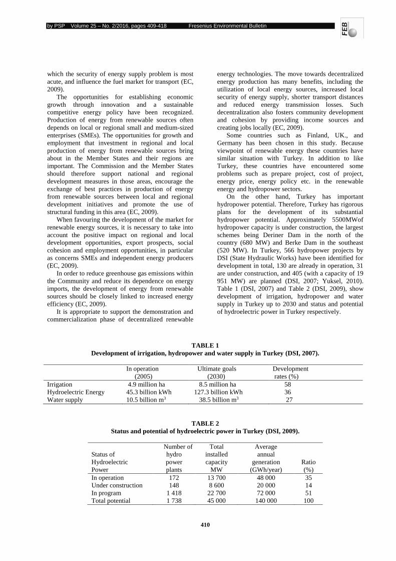
by PSP Volume 25 – No. 2/2016, pages 409-418 Fresenius Environmental Bulletin
410
which the security of energy supply problem is most
acute, and influence the fuel market for transport (EC,
2009).
The opportunities for establishing economic
growth through innovation and a sustainable
competitive energy policy have been recognized.
Production of energy from renewable sources often
depends on local or regional small and medium-sized
enterprises (SMEs). The opportunities for growth and
employment that investment in regional and local
production of energy from renewable sources bring
about in the Member States and their regions are
important. The Commission and the Member States
should therefore support national and regional
development measures in those areas, encourage the
exchange of best practices in production of energy
from renewable sources between local and regional
development initiatives and promote the use of
structural funding in this area (EC, 2009).
When favouring the development of the market for
renewable energy sources, it is necessary to take into
account the positive impact on regional and local
development opportunities, export prospects, social
cohesion and employment opportunities, in particular
as concerns SMEs and independent energy producers
(EC, 2009).
In order to reduce greenhouse gas emissions within
the Community and reduce its dependence on energy
imports, the development of energy from renewable
sources should be closely linked to increased energy
efficiency (EC, 2009).
It is appropriate to support the demonstration and
commercialization phase of decentralized renewable
energy technologies. The move towards decentralized
energy production has many benefits, including the
utilization of local energy sources, increased local
security of energy supply, shorter transport distances
and reduced energy transmission losses. Such
decentralization also fosters community development
and cohesion by providing income sources and
creating jobs locally (EC, 2009).
Some countries such as Finland, UK., and
Germany has been chosen in this study. Because
viewpoint of renewable energy these countries have
similar situation with Turkey. In addition to like
Turkey, these countries have encountered some
problems such as prepare project, cost of project,
energy price, energy policy etc. in the renewable
energy and hydropower sectors.
On the other hand, Turkey has important
hydropower potential. Therefore, Turkey has rigorous
plans for the development of its substantial
hydropower potential. Approximately 5500MWof
hydropower capacity is under construction, the largest
schemes being Deriner Dam in the north of the
country (680 MW) and Berke Dam in the southeast
(520 MW). In Turkey, 566 hydropower projects by
DSI (State Hydraulic Works) have been identified for
development in total, 130 are already in operation, 31
are under construction, and 405 (with a capacity of 19
951 MW) are planned (DSI, 2007; Yuksel, 2010).
Table 1 (DSI, 2007) and Table 2 (DSI, 2009), show
development of irrigation, hydropower and water
supply in Turkey up to 2030 and status and potential
of hydroelectric power in Turkey respectively.
TABLE 1
Development of irrigation, hydropower and water supply in Turkey (DSI, 2007).
In operation Ultimate goals Development
(2005) (2030) rates (%)
Irrigation 4.9 million ha 8.5 million ha 58
Hydroelectric Energy 45.3 billion kWh 127.3 billion kWh 36
Water supply 10.5 billion m3 38.5 billion m3 27
TABLE 2
Status and potential of hydroelectric power in Turkey (DSI, 2009).
Number of Total Average
Status of hydro installed annual
Hydroelectric power capacity generation Ratio
Power plants MW (GWh/year) (%)
In operation 172 13 700 48 000 35
Under construction 148 8 600 20 000 14
In program 1 418 22 700 72 000 51
Total potential 1 738 45 000 140 000 100
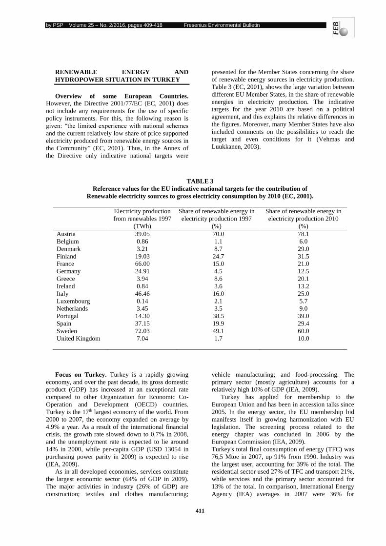
by PSP Volume 25 – No. 2/2016, pages 409-418 Fresenius Environmental Bulletin
411
RENEWABLE ENERGY AND
HYDROPOWER SITUATION IN TURKEY
Overview of some European Countries. However, the Directive 2001/77/EC (EC, 2001) does
not include any requirements for the use of specific
policy instruments. For this, the following reason is
given: “the limited experience with national schemes and the current relatively low share of price supported
electricity produced from renewable energy sources in
the Community” (EC, 2001). Thus, in the Annex of
the Directive only indicative national targets were
presented for the Member States concerning the share
of renewable energy sources in electricity production.
Table 3 (EC, 2001), shows the large variation between
different EU Member States, in the share of renewable
energies in electricity production. The indicative
targets for the year 2010 are based on a political
agreement, and this explains the relative differences in
the figures. Moreover, many Member States have also
included comments on the possibilities to reach the
target and even conditions for it (Vehmas and
Luukkanen, 2003).
TABLE 3
Reference values for the EU indicative national targets for the contribution of
Renewable electricity sources to gross electricity consumption by 2010 (EC, 2001).
Electricity production
from renewables 1997
(TWh)
Share of renewable energy in
electricity production 1997
(%)
Share of renewable energy in
electricity production 2010
(%)
Austria 39.05 70.0 78.1
Belgium 0.86 1.1 6.0
Denmark 3.21 8.7 29.0
Finland 19.03 24.7 31.5
France 66.00 15.0 21.0
Germany 24.91 4.5 12.5
Greece 3.94 8.6 20.1
Ireland 0.84 3.6 13.2
Italy 46.46 16.0 25.0
Luxembourg 0.14 2.1 5.7
Netherlands 3.45 3.5 9.0
Portugal 14.30 38.5 39.0
Spain 37.15 19.9 29.4
Sweden 72.03 49.1 60.0
United Kingdom 7.04 1.7 10.0
Focus on Turkey. Turkey is a rapidly growing
economy, and over the past decade, its gross domestic
product (GDP) has increased at an exceptional rate
compared to other Organization for Economic Co-
Operation and Development (OECD) countries.
Turkey is the 17th largest economy of the world. From
2000 to 2007, the economy expanded on average by
4.9% a year. As a result of the international financial
crisis, the growth rate slowed down to 0,7% in 2008,
and the unemployment rate is expected to lie around
14% in 2000, while per-capita GDP (USD 13054 in
purchasing power parity in 2009) is expected to rise
(IEA, 2009).
As in all developed economies, services constitute
the largest economic sector (64% of GDP in 2009).
The major activities in industry (26% of GDP) are
construction; textiles and clothes manufacturing;
vehicle manufacturing; and food-processing. The
primary sector (mostly agriculture) accounts for a
relatively high 10% of GDP (IEA, 2009).
Turkey has applied for membership to the
European Union and has been in accession talks since
2005. In the energy sector, the EU membership bid
manifests itself in growing harmonization with EU
legislation. The screening process related to the
energy chapter was concluded in 2006 by the
European Commission (IEA, 2009).
Turkey's total final consumption of energy (TFC) was
76,5 Mtoe in 2007, up 91% from 1990. Industry was
the largest user, accounting for 39% of the total. The
residential sector used 27% of TFC and transport 21%,
while services and the primary sector accounted for
13% of the total. In comparison, International Energy
Agency (IEA) averages in 2007 were 36% for
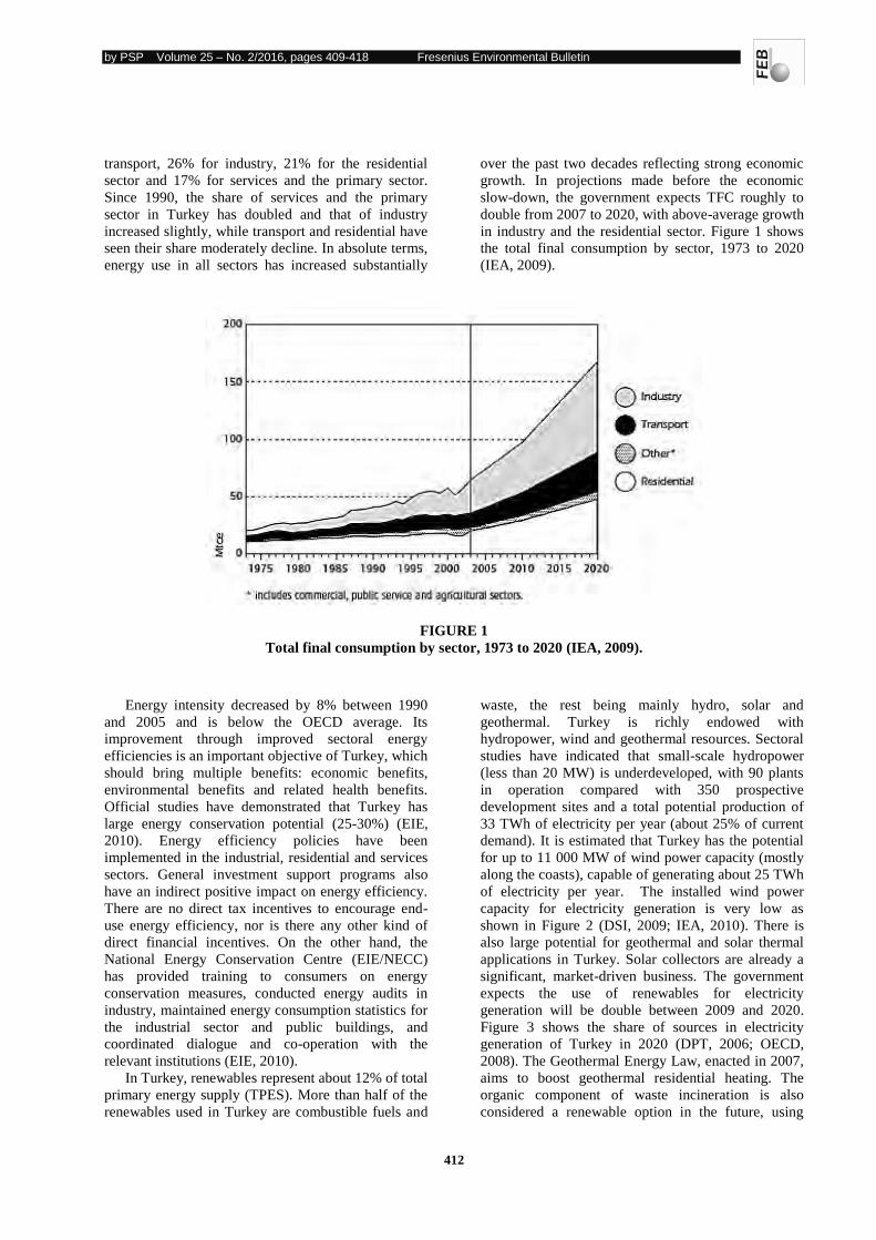
by PSP Volume 25 – No. 2/2016, pages 409-418 Fresenius Environmental Bulletin
412
transport, 26% for industry, 21% for the residential
sector and 17% for services and the primary sector.
Since 1990, the share of services and the primary
sector in Turkey has doubled and that of industry
increased slightly, while transport and residential have
seen their share moderately decline. In absolute terms,
energy use in all sectors has increased substantially
over the past two decades reflecting strong economic
growth. In projections made before the economic
slow-down, the government expects TFC roughly to
double from 2007 to 2020, with above-average growth
in industry and the residential sector. Figure 1 shows
the total final consumption by sector, 1973 to 2020
(IEA, 2009).
FIGURE 1
Total final consumption by sector, 1973 to 2020 (IEA, 2009).
Energy intensity decreased by 8% between 1990
and 2005 and is below the OECD average. Its
improvement through improved sectoral energy
efficiencies is an important objective of Turkey, which
should bring multiple benefits: economic benefits,
environmental benefits and related health benefits.
Official studies have demonstrated that Turkey has
large energy conservation potential (25-30%) (EIE,
2010). Energy efficiency policies have been
implemented in the industrial, residential and services
sectors. General investment support programs also
have an indirect positive impact on energy efficiency.
There are no direct tax incentives to encourage end-
use energy efficiency, nor is there any other kind of
direct financial incentives. On the other hand, the
National Energy Conservation Centre (EIE/NECC)
has provided training to consumers on energy
conservation measures, conducted energy audits in
industry, maintained energy consumption statistics for
the industrial sector and public buildings, and
coordinated dialogue and co-operation with the
relevant institutions (EIE, 2010).
In Turkey, renewables represent about 12% of total
primary energy supply (TPES). More than half of the
renewables used in Turkey are combustible fuels and
waste, the rest being mainly hydro, solar and
geothermal. Turkey is richly endowed with
hydropower, wind and geothermal resources. Sectoral
studies have indicated that small-scale hydropower
(less than 20 MW) is underdeveloped, with 90 plants
in operation compared with 350 prospective
development sites and a total potential production of
33 TWh of electricity per year (about 25% of current
demand). It is estimated that Turkey has the potential
for up to 11 000 MW of wind power capacity (mostly
along the coasts), capable of generating about 25 TWh
of electricity per year. The installed wind power
capacity for electricity generation is very low as
shown in Figure 2 (DSI, 2009; IEA, 2010). There is
also large potential for geothermal and solar thermal
applications in Turkey. Solar collectors are already a
significant, market-driven business. The government
expects the use of renewables for electricity
generation will be double between 2009 and 2020.
Figure 3 shows the share of sources in electricity
generation of Turkey in 2020 (DPT, 2006; OECD,
2008). The Geothermal Energy Law, enacted in 2007,
aims to boost geothermal residential heating. The
organic component of waste incineration is also
considered a renewable option in the future, using
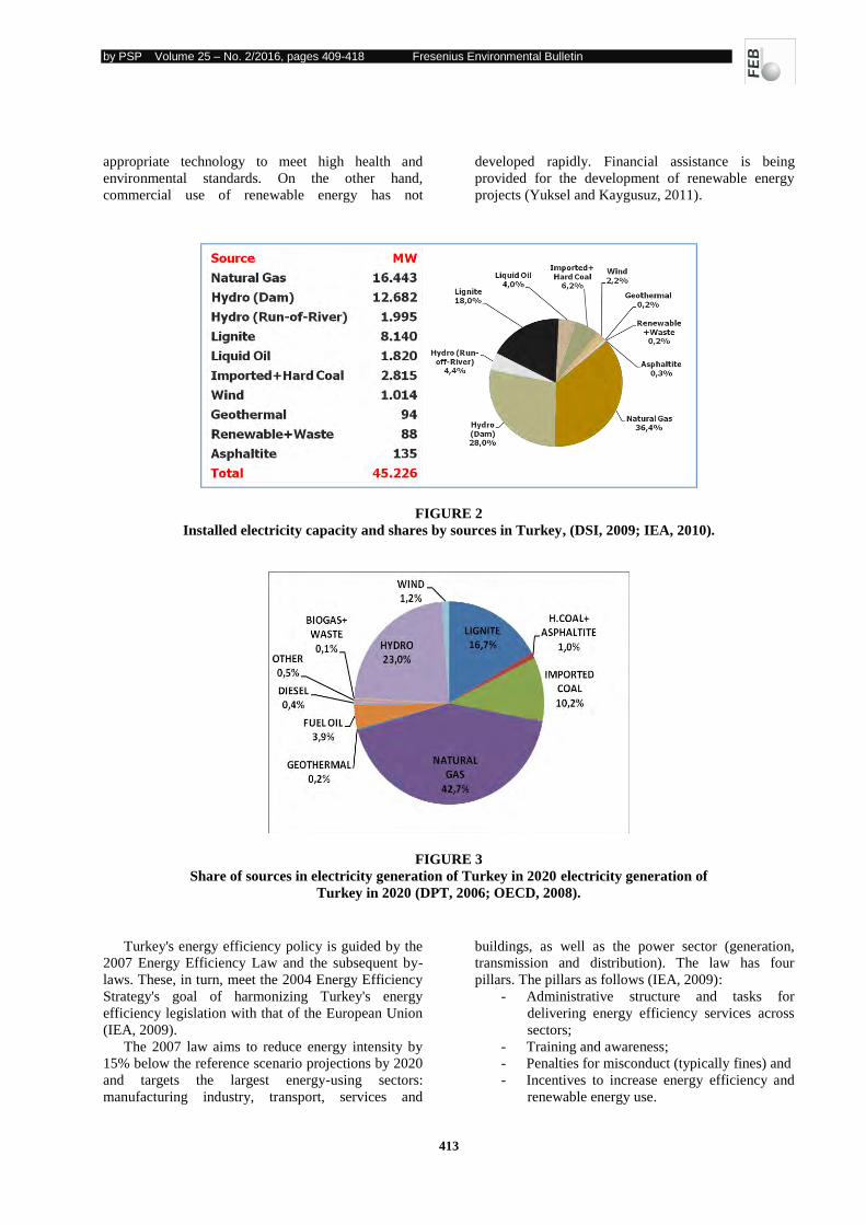
by PSP Volume 25 – No. 2/2016, pages 409-418 Fresenius Environmental Bulletin
413
appropriate technology to meet high health and
environmental standards. On the other hand,
commercial use of renewable energy has not
developed rapidly. Financial assistance is being
provided for the development of renewable energy
projects (Yuksel and Kaygusuz, 2011).
FIGURE 2
Installed electricity capacity and shares by sources in Turkey, (DSI, 2009; IEA, 2010).
FIGURE 3
Share of sources in electricity generation of Turkey in 2020 electricity generation of
Turkey in 2020 (DPT, 2006; OECD, 2008).
Turkey's energy efficiency policy is guided by the
2007 Energy Efficiency Law and the subsequent by-
laws. These, in turn, meet the 2004 Energy Efficiency
Strategy's goal of harmonizing Turkey's energy
efficiency legislation with that of the European Union
(IEA, 2009).
The 2007 law aims to reduce energy intensity by
15% below the reference scenario projections by 2020
and targets the largest energy-using sectors:
manufacturing industry, transport, services and
buildings, as well as the power sector (generation,
transmission and distribution). The law has four
pillars. The pillars as follows (IEA, 2009):
- Administrative structure and tasks for
delivering energy efficiency services across
sectors;
- Training and awareness;
- Penalties for misconduct (typically fines) and
- Incentives to increase energy efficiency and
renewable energy use.
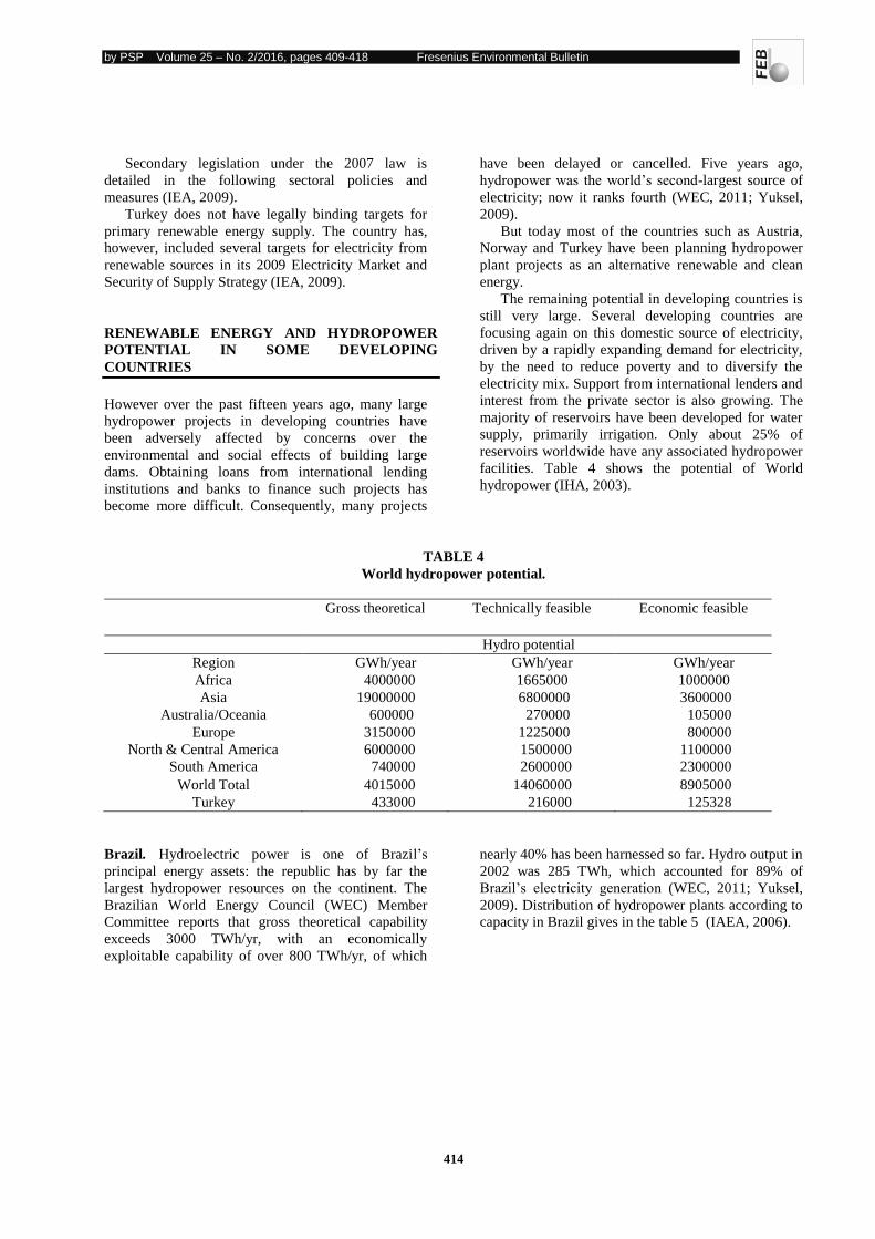
by PSP Volume 25 – No. 2/2016, pages 409-418 Fresenius Environmental Bulletin
414
Secondary legislation under the 2007 law is
detailed in the following sectoral policies and
measures (IEA, 2009).
Turkey does not have legally binding targets for
primary renewable energy supply. The country has,
however, included several targets for electricity from
renewable sources in its 2009 Electricity Market and
Security of Supply Strategy (IEA, 2009).
RENEWABLE ENERGY AND HYDROPOWER
POTENTIAL IN SOME DEVELOPING
COUNTRIES
However over the past fifteen years ago, many large
hydropower projects in developing countries have
been adversely affected by concerns over the
environmental and social effects of building large
dams. Obtaining loans from international lending
institutions and banks to finance such projects has
become more difficult. Consequently, many projects
have been delayed or cancelled. Five years ago,
hydropower was the world’s second-largest source of
electricity; now it ranks fourth (WEC, 2011; Yuksel,
2009).
But today most of the countries such as Austria,
Norway and Turkey have been planning hydropower
plant projects as an alternative renewable and clean
energy.
The remaining potential in developing countries is
still very large. Several developing countries are
focusing again on this domestic source of electricity,
driven by a rapidly expanding demand for electricity,
by the need to reduce poverty and to diversify the
electricity mix. Support from international lenders and
interest from the private sector is also growing. The
majority of reservoirs have been developed for water
supply, primarily irrigation. Only about 25% of
reservoirs worldwide have any associated hydropower
facilities. Table 4 shows the potential of World
hydropower (IHA, 2003).
TABLE 4
World hydropower potential.
Gross theoretical Technically feasible Economic feasible
Hydro potential
Region GWh/year GWh/year GWh/year
Africa 4000000 1665000 1000000
Asia 19000000 6800000 3600000
Australia/Oceania 600000 270000 105000
Europe 3150000 1225000 800000
North & Central America 6000000 1500000 1100000
South America 740000 2600000 2300000
World Total 4015000 14060000 8905000
Turkey 433000 216000 125328
Brazil. Hydroelectric power is one of Brazil’s principal energy assets: the republic has by far the
largest hydropower resources on the continent. The
Brazilian World Energy Council (WEC) Member
Committee reports that gross theoretical capability
exceeds 3000 TWh/yr, with an economically
exploitable capability of over 800 TWh/yr, of which
nearly 40% has been harnessed so far. Hydro output in
2002 was 285 TWh, which accounted for 89% of
Brazil’s electricity generation (WEC, 2011; Yuksel,
2009). Distribution of hydropower plants according to
capacity in Brazil gives in the table 5 (IAEA, 2006).
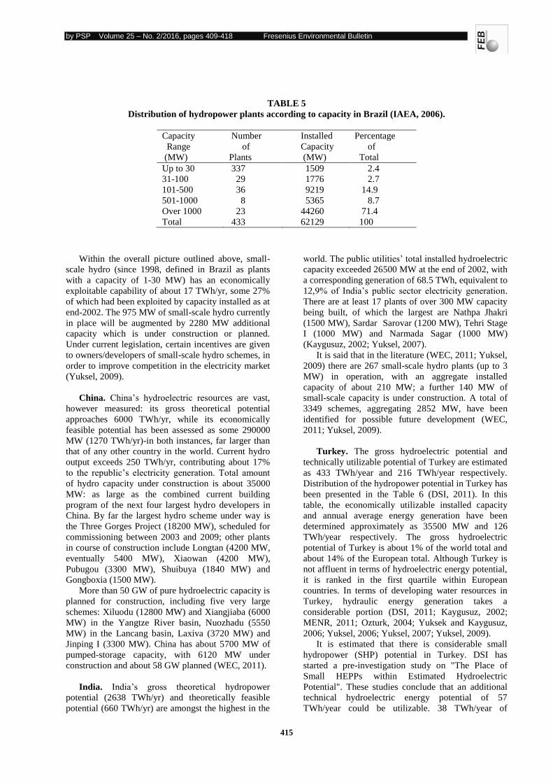
by PSP Volume 25 – No. 2/2016, pages 409-418 Fresenius Environmental Bulletin
415
TABLE 5
Distribution of hydropower plants according to capacity in Brazil (IAEA, 2006).
Capacity Number Installed Percentage
Range of Capacity of
(MW) Plants (MW) Total
Up to 30 337 1509 2.4
31-100 29 1776 2.7
101-500 36 9219 14.9
501-1000 8 5365 8.7
Over 1000 23 44260 71.4
Total 433 62129 100
Within the overall picture outlined above, small-
scale hydro (since 1998, defined in Brazil as plants
with a capacity of 1-30 MW) has an economically
exploitable capability of about 17 TWh/yr, some 27%
of which had been exploited by capacity installed as at
end-2002. The 975 MW of small-scale hydro currently
in place will be augmented by 2280 MW additional
capacity which is under construction or planned.
Under current legislation, certain incentives are given
to owners/developers of small-scale hydro schemes, in
order to improve competition in the electricity market
(Yuksel, 2009).
China. China’s hydroelectric resources are vast,
however measured: its gross theoretical potential
approaches 6000 TWh/yr, while its economically
feasible potential has been assessed as some 290000
MW (1270 TWh/yr)-in both instances, far larger than
that of any other country in the world. Current hydro
output exceeds 250 TWh/yr, contributing about 17%
to the republic’s electricity generation. Total amount of hydro capacity under construction is about 35000
MW: as large as the combined current building
program of the next four largest hydro developers in
China. By far the largest hydro scheme under way is
the Three Gorges Project (18200 MW), scheduled for
commissioning between 2003 and 2009; other plants
in course of construction include Longtan (4200 MW,
eventually 5400 MW), Xiaowan (4200 MW),
Pubugou (3300 MW), Shuibuya (1840 MW) and
Gongboxia (1500 MW).
More than 50 GW of pure hydroelectric capacity is
planned for construction, including five very large
schemes: Xiluodu (12800 MW) and Xiangjiaba (6000
MW) in the Yangtze River basin, Nuozhadu (5550
MW) in the Lancang basin, Laxiva (3720 MW) and
Jinping I (3300 MW). China has about 5700 MW of
pumped-storage capacity, with 6120 MW under
construction and about 58 GW planned (WEC, 2011).
India. India’s gross theoretical hydropower
potential (2638 TWh/yr) and theoretically feasible
potential (660 TWh/yr) are amongst the highest in the
world. The public utilities’ total installed hydroelectric
capacity exceeded 26500 MW at the end of 2002, with
a corresponding generation of 68.5 TWh, equivalent to
12,9% of India’s public sector electricity generation.
There are at least 17 plants of over 300 MW capacity
being built, of which the largest are Nathpa Jhakri
(1500 MW), Sardar Sarovar (1200 MW), Tehri Stage
I (1000 MW) and Narmada Sagar (1000 MW)
(Kaygusuz, 2002; Yuksel, 2007).
It is said that in the literature (WEC, 2011; Yuksel,
2009) there are 267 small-scale hydro plants (up to 3
MW) in operation, with an aggregate installed
capacity of about 210 MW; a further 140 MW of
small-scale capacity is under construction. A total of
3349 schemes, aggregating 2852 MW, have been
identified for possible future development (WEC,
2011; Yuksel, 2009).
Turkey. The gross hydroelectric potential and
technically utilizable potential of Turkey are estimated
as 433 TWh/year and 216 TWh/year respectively.
Distribution of the hydropower potential in Turkey has
been presented in the Table 6 (DSI, 2011). In this
table, the economically utilizable installed capacity
and annual average energy generation have been
determined approximately as 35500 MW and 126
TWh/year respectively. The gross hydroelectric
potential of Turkey is about 1% of the world total and
about 14% of the European total. Although Turkey is
not affluent in terms of hydroelectric energy potential,
it is ranked in the first quartile within European
countries. In terms of developing water resources in
Turkey, hydraulic energy generation takes a
considerable portion (DSI, 2011; Kaygusuz, 2002;
MENR, 2011; Ozturk, 2004; Yuksek and Kaygusuz,
2006; Yuksel, 2006; Yuksel, 2007; Yuksel, 2009).
It is estimated that there is considerable small
hydropower (SHP) potential in Turkey. DSI has
started a pre-investigation study on "The Place of
Small HEPPs within Estimated Hydroelectric
Potential". These studies conclude that an additional
technical hydroelectric energy potential of 57
TWh/year could be utilizable. 38 TWh/year of
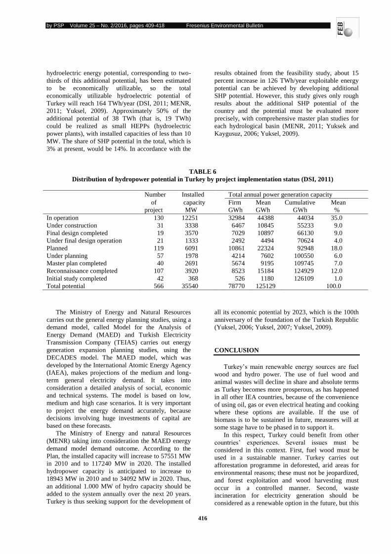
by PSP Volume 25 – No. 2/2016, pages 409-418 Fresenius Environmental Bulletin
416
hydroelectric energy potential, corresponding to two-
thirds of this additional potential, has been estimated
to be economically utilizable, so the total
economically utilizable hydroelectric potential of
Turkey will reach 164 TWh/year (DSI, 2011; MENR,
2011; Yuksel, 2009). Approximately 50% of the
additional potential of 38 TWh (that is, 19 TWh)
could be realized as small HEPPs (hydroelectric
power plants), with installed capacities of less than 10
MW. The share of SHP potential in the total, which is
3% at present, would be 14%. In accordance with the
results obtained from the feasibility study, about 15
percent increase in 126 TWh/year exploitable energy
potential can be achieved by developing additional
SHP potential. However, this study gives only rough
results about the additional SHP potential of the
country and the potential must be evaluated more
precisely, with comprehensive master plan studies for
each hydrological basin (MENR, 2011; Yuksek and
Kaygusuz, 2006; Yuksel, 2009).
TABLE 6
Distribution of hydropower potential in Turkey by project implementation status (DSI, 2011)
Number Installed Total annual power generation capacity
of capacity Firm Mean Cumulative Mean
project MW GWh GWh GWh %
In operation 130 12251 32984 44388 44034 35.0
Under construction 31 3338 6467 10845 55233 9.0
Final design completed 19 3570 7029 10897 66130 9.0
Under final design operation 21 1333 2492 4494 70624 4.0
Planned 119 6091 10861 22324 92948 18.0
Under planning 57 1978 4214 7602 100550 6.0
Master plan completed 40 2691 5674 9195 109745 7.0
Reconnaissance completed 107 3920 8523 15184 124929 12.0
Initial study completed 42 368 526 1180 126109 1.0
Total potential 566 35540 78770 125129 100.0
The Ministry of Energy and Natural Resources
carries out the general energy planning studies, using a
demand model, called Model for the Analysis of
Energy Demand (MAED) and Turkish Electricity
Transmission Company (TEIAS) carries out energy
generation expansion planning studies, using the
DECADES model. The MAED model, which was
developed by the International Atomic Energy Agency
(IAEA), makes projections of the medium and long-
term general electricity demand. It takes into
consideration a detailed analysis of social, economic
and technical systems. The model is based on low,
medium and high case scenarios. It is very important
to project the energy demand accurately, because
decisions involving huge investments of capital are
based on these forecasts.
The Ministry of Energy and natural Resources
(MENR) taking into consideration the MAED energy
demand model demand outcome. According to the
Plan, the installed capacity will increase to 57551 MW
in 2010 and to 117240 MW in 2020. The installed
hydropower capacity is anticipated to increase to
18943 MW in 2010 and to 34092 MW in 2020. Thus,
an additional 1.000 MW of hydro capacity should be
added to the system annually over the next 20 years.
Turkey is thus seeking support for the development of
all its economic potential by 2023, which is the 100th
anniversary of the foundation of the Turkish Republic
(Yuksel, 2006; Yuksel, 2007; Yuksel, 2009).
CONCLUSION
Turkey’s main renewable energy sources are fuel
wood and hydro power. The use of fuel wood and
animal wastes will decline in share and absolute terms
as Turkey becomes more prosperous, as has happened
in all other IEA countries, because of the convenience
of using oil, gas or even electrical heating and cooking
where these options are available. If the use of
biomass is to be sustained in future, measures will at
some stage have to be phased in to support it.
In this respect, Turkey could benefit from other
countries’ experiences. Several issues must be considered in this context. First, fuel wood must be
used in a sustainable manner. Turkey carries out
afforestation programme in deforested, arid areas for
environmental reasons; these must not be jeopardized,
and forest exploitation and wood harvesting must
occur in a controlled manner. Second, waste
incineration for electricity generation should be
considered as a renewable option in the future, but this
by PSP Volume 25 – No. 2/2016, pages 409-418 Fresenius Environmental Bulletin
417
should be done using appropriate technology to ensure
high health and environmental standards, in particular
with respect to air emissions (IEA, 2001).
On the other hand, hydropower has an extensive
list of positive characteristics. In addition to power
generation and efficiency, it has advantages such as:
flood protection, flow regulation, fossil fuel
avoidance, a long depreciation period, revenue by an
adequate electricity rate, and low operating–maintenance–replacement costs. In addition, hydro
plants are often superior to other power plants from
the standpoint of socio-economic and environmental
considerations (IHA, 2003; IEA, 2002; IEA, 2003;
WEC, 2011; Yuksel, 2008).
In addition to the environmental impacts of
hydropower plants are at the lowest level compared
with the other alternative resources. They make use of
our renewable ‘‘green energy’’ resource, without causing pollution and CO2 emission. They have
considerable advantages; since they use the renewable
sources of the country, are free of fuel costs and their
design and construction can be performed by Turkish
engineers and contractors. They are also easily
adaptable to the system load demands (IHA, 2003;
Yuksel, 2008). The advantages of hydropower as
follows:
• A sustainable resource: It meets the needs of the
present without compromising the ability of future
generations to meet their own needs.
• An efficient resource: It can satisfy energy demand
with no depletion of the resource and with little impact
on the environment.
• A secure resource: Small hydropower is available
within the borders of one country and is not subject to
disruption by international political events. This
guarantees its security of supply.
• A clean resource: It does not involve a process of
combustion, thus avoiding pollution and greenhouse
gas emissions.
• A renewable resource: The fuel for hydropower is
water, which is not consumed in the electricity
generation process.
In this case, it is important to point out the
restructuring policies that are directing the
development of new and renewable energy, and giving
special emphasis to socio-economical bodies, laws and
legal regulations. In this respect, particular attention
and priority should be given to the development of the
hydroelectric potential in Turkey, since it is the most
important natural renewable resource and only 35% of
the technically and economically utilizable hydro
potential has been developed so far (IHA, 2003;
MENR, 2011; Yuksel, 2008).
On the other hand in the last decades, some
countries including Turkey have been planning large
or small hydropower projects as an alternative
renewable energy instead of fuel, biomass and
geothermal.
REFERENCES
[1] Dinica, V., United Kingdom. In: Reiche, D.
(ed.), “Handbook of Renewable Energies in the
European Union Case studies of all Member
States.” Peter Lang, Frankfurt 2002. [2] DPT, State Planning Organization. Ninth
Development plan 2007–2013, Ankara, Turkey,
2006.
[3] DSI, State Water Works. Hydropower potential
in Turkey, Ankara, Turkey, 2007.
[4] DSI, State Water Works. Turkey water report,
Ankara, Turkey, 2009.
[5] DSI, State Hydraulic Works, “Statistics on hydropower”, Ankara, Turkey, www.dsi.gov.tr,
accessed date 16 March 2011.
[6] EC, European Countries, Directive 2001/77/EC
of the European Parliament and the Council of
27 September 2001 on the promotion of
electricity produced from renewable energy
sources in the internal electricity market, Official
Journal of the European Communities, L283/35,
2001.
[7] EC, European Countries, Directive 2009/28/EC
of the European Parliament and the Council of
23 April 2009 on the promotion of the use of
energy from renewable sources and amending
and subsequently repealing Directives
2001/77/EC and 2003/30/EC, (Text with EEA
relevance), Official Journal of the European
Union, 2009.
[8] EIE, Electrical Power Resources Survey and
Development Administration. Renewable energy
activities of the EIE, 2009, http://www.eie.gov.tr/
(accessed 12.08.2010).
[9] IAEA, International Atomic Energy Agency,
“Brazil: A Country Profile on Sustainable
Energy Development”, Vienna, Austria, 2006.
[10] IEA, International Energy Agency, “Energy Policies of IEA Countries 2001 Review.” IEA, Paris, 2001.
[11] IEA, International Energy Agency, “Renewable Information 2002 with 2000 data”, IEA, Paris, 2002.
[12] IEA, International Energy Agency, “Energy Balances of OECD Countries”, IEA, Paris, 2003.
[13] IEA, International Energy Agency, “Energy Policies of IEA Countries 2009 Review”, IEA, Paris, 2009.
[14] IHA, International Hydropower Association,
“The Role of Hydropower in Sustainable
Development”, IHA White Paper, 2003.
by PSP Volume 25 – No. 2/2016, pages 409-418 Fresenius Environmental Bulletin
418
[15] Kaygusuz, K., “Sustainable Development of Hydropower”, Energy Sources. 24 (2002) 803-
815.
[16] MEF, Ministry of Environment and Forestry
First national Communication of Turkey on
Climate Change (Eds. Apak, G and Ubay, B), pp.
60-150, Ankara, Turkey, 2007
[17] MENR, Ministry of Energy and Natural
Resources. “Energy report of Turkey in 2008”
[18] MENR, Ministry of Energy and Natural
Resources, “Energy Statistics of Turkey in
2005”, Available from http://www.menr.gov.tr,
accessed date 10 April 2011.
[19] OECD, Organisation for Economic Co-
Operation and development. Environmen-tal
performance reviews: Turkey. Paris: OECD;
2008.
[20] Ozturk, R. and Kıncay, O., “Potential of Hydroelectric Energy”, Energy Sources. 26 (2004) 1141-1156.
[21] Reiche, D., “Renewable energies in the EU Member States in comparison”, In: Reiche, D.
(Ed.), Handbook of Renewable Energies in the
European Union, Case Studies of all Member
States, Frankfurt, 2002.
[22] WEC, World Energy Council, “Survey of Energy Resources”, www.worldenergy.org, access date
05 April 2011.
[23] Vehmas, J. and Luukkanen, J., Finland. In:
Reiche, D. (ed.), “Handbook of Renewable
Energies in the European Union Case studies of
all Member States.” Peter Lang, Frankfurt, 2002.
[24] Vehmas, J. and Luukkanen, J., “Renewable Energies in the European Union and Turkey” Energy Policy of the EU and Implications for
Turkey - Conference/Workshop Vehmas and
Luukkanen, 2003.
[25] Yuksek, O and Kaygusuz, K., “Small Hydropower Plants As a New and Renewable
Energy Source”, Energy Sources, Part B. 1
(2006) 279-290.
[26] Yuksel, I., “Southeastern Anatolia Project (GAP) for Irrigation and Hydroelectric Power in
Turkey”, Energy Exploration & Exploitation. 24
(2006) 361-370.
[27] Yuksel, I., “Development of Hydropower: A Case Study in Developing Countries”, Energy Sources, Part B. 2 (2007) 113-121.
[28] Yuksel., I., Hydropower in Turkey for a clean
and sustainable energy future Renewable and
Sustainable Energy Reviews. 12 (2008) 1622–1640.
[29] Yuksel, I., “Hydroelectric Power in Developing Countries”, Energy Sources, Part B: Economics,
Planning, and Policy. 4 (2009) 377-386.
[30] Yuksel, I., “Hydropower for Sustainable Water
and Energy Development”, Journal of
Renewable and Sustainable Energy Reviews. 14
(2010) 462 - 469.
[31] Yuksel, I and Kaygusuz, K., “Renewable energy sources for clean and sustainable energy policies
in Turkey” Renewable and Sustainable Energy
Reviews. 15 (2011) 4132- 4144.
Received: 11.06.2015
Accepted: 18.01.2016
CORRESPONDING AUTHOR
Ibrahim Yuksel
Yildiz Technical University
Civil Engineering Faculty
Department of Civil Engineering
Hydraulics Division
34220 Davutpasa-Istanbul – TURKEY
e-mail: [email protected]
by PSP Volume 25 – No. 2/2016, pages 419-428 Fresenius Environmental Bulletin
419
RESEARCH ON VEGETATION ECOLOGICAL RISK
ASSESSMENT BASED ON RRM-TAKE XIANGXI RIVER
HYDRO-FLUCTUATION BELT OF THREE GORGES
RESERVOIR AREA AS AN EXAMPLE
Haiyan Li1, Peijiang Zhou1, Chao Xu1, Wanshun Zhang1, Guoqiang Song2
1School of Resource and Environmental Science, Wuhan University, 430079, Wuhan, China
2Hubei Academy of Environmental Sciences , Bayi Road, 430079, Wuhan, China
ABSTRACT
This paper assesses the vegetation risk of
different risk areas and various vegetations
respectively based on improved relative risk
assessment model RRM taking Xiangxi river
hydro-fluctuation belt as an example. The
ecological risk assessment technology system of
risk degree- vulnerability-loss degree is also
constructed on the basis of multiple risk sources
and multiple receptors. It also introduces the
concept of anti-interference index to analysis the
expose-response relationship between risk sources
and receptors. The results show that:(1) The current
vegetation ecological risk in Xiangxi river hydro-
fluctuation belt stays at moderate risk degree, and
then the low risk area, the high risk area has a lower
proportion. (2)The risk grade of various vegetations
are arbor vegetation, brush vegetation, grass
vegetation and farmland vegetation by descending
order. (3) Herbaceous plants with strong
adaptability should be chosen to repair the
ecological environment which has higher flood
resistance and lower risk in area below 160m. In the
area between 150m and 160m reasonable utilization
of land could be a effective measure to reduce the
vegetation risk.
KEY WORDS:
Three Gorges Reservoir Area, Xiangxi River Hydro-
fluctuation Belt, Multiple Risk Sources, Vegetation
Ecological Risk Assessment, RRM
INTRODUCTION
The ecological risk assessment study
experiences the development process from
environment risk to ecological risk and then area
ecological risk assessment, the risk source expands
from single risk source to multiple risk sources, the
risk receptor expands from single receptor to
multiple receptors, as well as the assessment scope
expands from local area to area landscape [1,2] in
several decades. Currently, vegetation risk
assessment method includes RRM method, vague
comprehensive assessment[3], artificial neuron
network method[4], as well as the method based on
RS and GIS technology risk assessment [5,6]. Dai,
BL (Dai, Benlin) [7] evaluated the surface water
quality of Emei river in China. In the research an
improved method (PPM-PCAM) which combines
projection pursuit model (PPM) with principal
component analysis method (PCAM) was
developed for use in this study. An EFR assessment
model was developed based on both the spatial
structure and the dominant eco-function of the river
ecosystem in the Haihe River Basin in the study of
Yang, T (Yang, Tao) [8]. RRM pattern was put
forward by Landis and Wiegers since 1997, by
which the multiple risk sources and multiple end
points can be well combined together through
setting grades [9]. Such model is widely used in
regional risk assessment, land utilization risk, water
environment and ecology risk.
The hydro-fluctuation belt is formed between
145m and 175m area after water storage of three
gorges reservoir area, among which most of them
are hard rock typed hill hydro-fluctuation belts with
sparse vegetation. Therefore, the structure and
function changes of the vegetation in hydro-
fluctuation belt have important ecological
significance, which has arisen the attention of the
researchers in both ecology and environment
science daily. Currently, researches on vegetation
ecological risk mainly focus on basin scale with
less attention on hydro-fluctuation belts. Therefore,
this paper tries to improve the RRM model in the
following ways in the process of vegetation
ecological risk assessment of hydro-fluctuation
belts. This paper on one hand references to
application of the RRM [10-13] on basin ecological
risk assessment, on the other it introduces anti-
interference index from the angle of vegetation
ecology. The vulnerability of the environment and
each vegetation ecological system are both
considered which can reduce the inaccuracy in
by PSP Volume 25 – No. 2/2016, pages 419-428 Fresenius Environmental Bulletin
420
vulnerability degree assessment. The evaluation
index system for risk degree and vulnerability
degree are also proposed according to the situation
of hydro-fluctuation belts.
RESEARCH AREA
Xiangxi river locates in the west of Hubei
province and the north of Xiling Gorge of Yangtze
The research scope of this paper mainly involves
the hydro-fluctuation belt in Xingshan and Zigui
counties of Yichang city with area of 8.19km2.
Xiangxi river hydro-fluctuation belt basically with a
steep slope and serious soil erosions. The anti-
seasonal and cyclical fluctuation phenomenon of
the level water aggravates the soil erosion and rock
exposure, which caused the vegetation cannot
survive and appears “desertification liked” situation. According to the field investigation and
document statistics data analysis [14,15], great
changes take place on vegetation quantity in the
hydro-fluctuation belt after impoundment, which
reduces 26 branches and 83 types. Therefore, the
richness and the diversity of species dramatically
decreased in the hydro-fluctuation belt of Xiangxi
river where herbaceous plant can survive and
setaria macrostachya is widely distributed. With the
increase of the altitude, the exposure area of the
hydro-fluctuation belt increases gradually, and the
richness and diversity of the vegetation species
improves gradually.
MATERIALS AND METHODS
Risk assessment receptor choosing of the
hydro-fluctuation belt
Receptor refers to the risk taker in the
ecological system who suffered from risk source
during risk assessment process, it may be organism
or non-organism[16].The key species, population,
community and ecosystem-types are usually chosen
as the risk receptor which are sensitive to the risk
factor or has significant consequences in ecosystem.
As hydro-fluctuation belt ecological system is
the interlace belt of the land and water ecological
system wetlands ecosystem is formed gradually
which leads to the vegetation type and community
successions. Vegetation ecosystem can keep the soil
stable, prevent surface erosion, stabilize bank,
intercept organics, such as chemical fertilizers and
pesticides, which reflect the influences and changes
on ecosystem structures and functions. The bear
ability to ecological risk is significantly difference
among different vegetation types, so we choose
arbor vegetation, shrub vegetation, herbal
vegetation and farmland vegetation as ecological
risk receptors.
Risk source analysis. Firstly, according to the
graded distribution characteristics of the Xiangxi
river hydro-fluctuation, it is classified to four risk
area: areaⅠ bellow 150m , area 150m-
160m , area (160m-170m) and area (above
170m). The elevation and water level have
important effects to the vegetation population
distribution. The anti-season and drowned type
changes the soil physical and chemical properties,
which intensifies soil erosion and the increase of
soil and water loss, and then the soil layer becomes
thinner leading to the richness of the species
reduced. Besides, based on the research on the
effects of water level fluctuations on the wetland
landscape , it influenced greatly the structure and
composition of the landscape and the dynamic
response of the waterfowl habitat areas to water
level fluctuations was presented [17].Therefore, in
view of the greatly influence on landscape of water
level it was selected as an important evaluation
factor. The frequent occurrence of the geological
disaster also leads to the species reduction.
Xingshan and Zigui are the prone areas of the
natural geological disaster. Therefore slide slope
stabilized factor is chosen to indicate the possibility
of the slide slope occurrence. The utilization of the
fertilizer changes the N/P ratio in the soil which
influences the species composition and life form
and then the distribution pattern will be different.
The characteristics of phosphorus adsorption onto
soils have been studied in Danjiangkou reservoir
[18]. In the study samples of soil in five different
land uses (cropland, forest land, abandon cropland,
grass land, orange orchard) were taken in the
elevations of 160m, 165m and 170m. And the
characteristics of phosphorus adsorption onto soils
are different by different land uses. The risk degree
assessment indexes of hydro-fluctuation belt risk
source are list in table 2-1.
The risk degree index is introduced to
characterize the probability and intensity of the risk
source which calculated by Analytic Hierarchy
Process(AHP). And due to multiple risk sources
characteristics the relative weight factor is also
introduced to distinguish risk degree of different
risk sources in various risk areas [10]. The
calculation formula is as follows:
ij
n
i
iji whH 1
1
by PSP Volume 25 – No. 2/2016, pages 419-428 Fresenius Environmental Bulletin
421
Where, Hi is the degree index in risk areas i,
hij is risk index of risk sources j in risk area i, wij is
the weight of risk source j in risk area i.
Exposure and response analysis. The anti-
interference index reflects the buffer and adjusting
ability of ecosystem in different various risk units,
fragile index is used to reflect vulnerability of
different ecosystem in various risk units and the
ecological loss index indicates the differences of
ecological damage suffered from the disaster.
Anti-interference index. Anti-interference
index includes: specie richness index, diversity
index and the area proportion of ecological system.
The calculation formula is as follows:
ij
i
ij eE
3
1
j 2
Where, Eij is the anti-interference index of
vegetation ecosystem j in risk area i, λj is the weight
of factor j, eij is the normalized value of factor j.
Vulnerability index calculation. The
ecological environment vulnerability of one area is
changing gradually under outside environment
influences [19,20]. As ecological environment is
influenced by both human and nature factors, we
choose ecological factors and human factors to
construct the vulnerability assessment index system
based on the domestic research achievements
[10,11]. The calculation formula is as follows:
j
n
i
iij EVwPV
i
1
3
Where, Vij is vulnerability index of vegetation
ecosystem j in risk area I, Pi is the normalized value
of factor I, wi is the weight of factor I, n is The
number of evaluation index, EVj is Fragile index of
Vegetation ecosystem j;
Specific assessment indexes system are list in
table 2-2.
On the basis of referring the present research [13], arbor, brush, herbaceous vegetation and
farmland vegetation are given different values
respectively, arbor assignment 4, brush assignment
3, grass assignment1 and farmland vegetation
assignment 2.
TABLE 2-1
Risk degree evaluation index system of Hydro-Fluctuation Belt
Risk source Elements Indicators The index type
water loss and soil
erosion
Rainfall intensity Average annual rainfall Positive
Soil erosion fators[15] slope Positive
Vegetation factor The vegetation coverage Reverse
Terrain LS Positive
Water level Flooding time Flooding time Positive
Geological disaster Landslide [16] Stability coefficients Reverse
human disturbance Farming Fertilizer runoff Positive
Phosphate enterprises Phosphorus loss Positive
Ecological loss degree calculation.
Ecological loss degree means the changing degree
of ecological system structures, functions and
others after risk receptor exposing under risk
sources. Ecological loss degree calculation formula
is as follows:
ijijj VEEDi 4
Where, EDij is the loss degree of vegetation
ecosystem j in risk area I, Eij is the anti-interference
index of Vegetation ecosystem j in Risk area I, Vij is
vulnerability index of vegetation ecosystem j
in Risk area i.
Comprehensive ecological risk value
calculation. Risk value is the indication of the
ecological risk which should include risk source
strength, occurrence possibility, risk receptor
characteristics, the impact of risk source to risk
receptor and other information. The detailed
calculation model is as follow:
iijij HEDR 5
by PSP Volume 25 – No. 2/2016, pages 419-428 Fresenius Environmental Bulletin
422
Where, Rij is ecological risk value of
vegetation ecosystem j in risk area i, EDij is the loss
degree of vegetation ecosystem j in risk area i, Hij is
risk degree index of vegetation ecosystem j in risk
area i.
i
i
iji wRCR
4
1
6
Where, CRi is comprehensive ecological risk
value of risk area i, Rij is ecological risk value of
vegetation ecosystem j in risk area i, wi is the
weight of factor i.
RESULTS AND ANALYSIS
Risk degree of various risk sources. Because
of the different dimension, the above value should
be normalization processed to get risk index of each
risk source. Each risk degree index of each risk area
can be obtained by formula (1) which is shown in
table 3-1.
TABLE 2-2
The vulnerability assessment index system of different habitat
TABLE 3-1
Risk evaluation index of various risk area of Hydro-Fluctuation Bel
Table 3-1 and figure1 shows that: the risk area
risk degree are area , area , area and area
by descending order. Water level risk mainly
distributes in Area and accounting for 74%,
which have longer drowned time, slide slope risk
occurrence possibility is higher. Owing to the
bigger gradient and intense human disturbance has
plus bigger people interference, the risk degree
index in area is higher than it in area .
Analyzing from different risk area, the main risk
source of area and area are drowned time and
geography disaster risk. The major risk source in
area are geography disaster risk and human
interference. Soil erosion risk mainly scatteres in
the area above 160m which is converted to
farmland whose agriculture soil erosion rate is
greater than other types of vegetation, and water
loss and soil erosion is easy to happen. It has a
larger gradient and higher flush caused by erosive
rain, and the vegetation has lower inhibitory action
in the area above 170m of which the soil erosion
risk level is higher. The effective actions should be
proposed according to different risk sources and
risk areas to reduce the risk level. The species with
high waterlogging tolerance should be screened out
and cultivated which can survive in area and
Risk source Elements Indicators The index type
Ecological factors
geological
elevation Positive
slope Positive
The soil corrosion factor K Positive
Geological disasters Positive
meteorological Erosive rainfall frequency Positive
The earth's surface factor The vegetation coverage Reverse
drainage Flooding time Positive
Social factors Pollutant emission intensity Point source discharge Positive
Non-point source emissions Positive
Risk area Water level
index
soil and water
loss Index
Geological
hazard index
Human disturbance
index
Comprehensive
risk
Area 0.42 0.12 0.33 0.14 0.31
Area 0.32 0.08 0.38 0.17 0.27
Area 0.16 0.13 0.24 0.30 0.19
Area 0.11 0.67 0.05 0.39 0.23
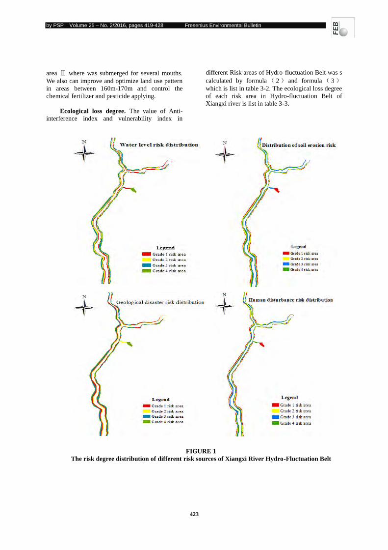
by PSP Volume 25 – No. 2/2016, pages 419-428 Fresenius Environmental Bulletin
423
area where was submerged for several mouths.
We also can improve and optimize land use pattern
in areas between 160m-170m and control the
chemical fertilizer and pesticide applying.
Ecological loss degree. The value of Anti-
interference index and vulnerability index in
different Risk areas of Hydro-fluctuation Belt was s
calculated by formula 2 and formula 3
which is list in table 3-2. The ecological loss degree
of each risk area in Hydro-fluctuation Belt of
Xiangxi river is list in table 3-3.
FIGURE 1
The risk degree distribution of different risk sources of Xiangxi River Hydro-Fluctuation Belt
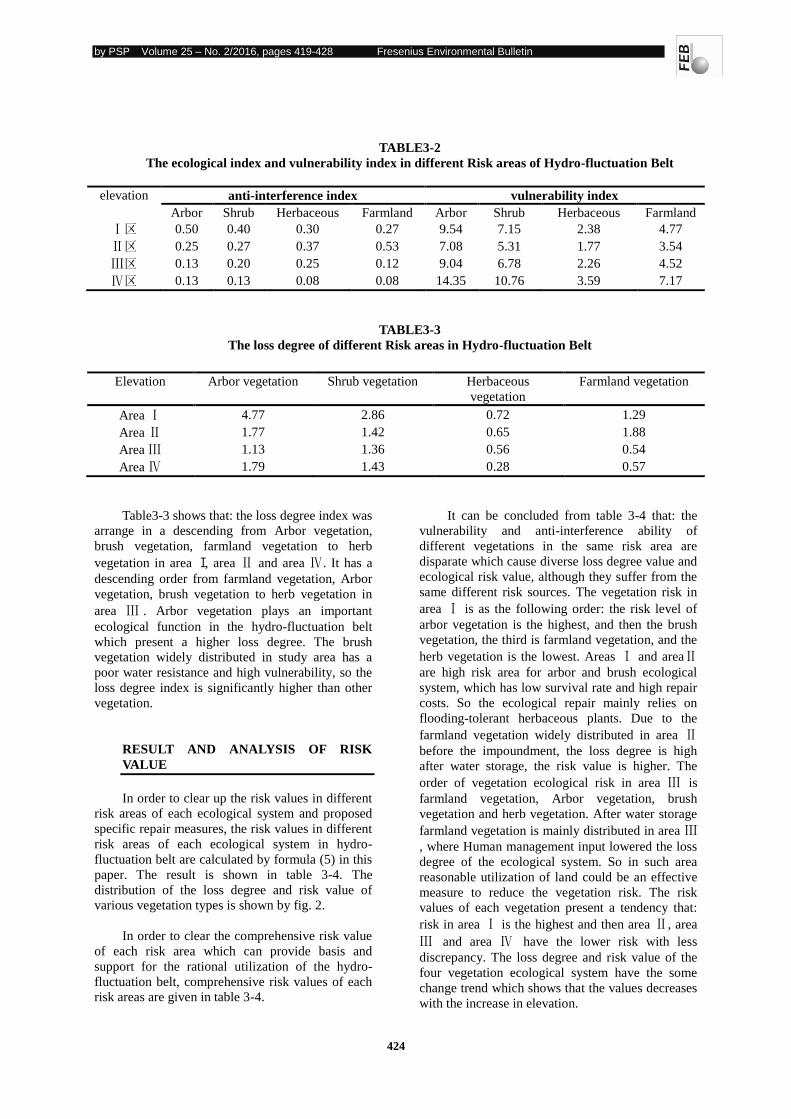
by PSP Volume 25 – No. 2/2016, pages 419-428 Fresenius Environmental Bulletin
424
TABLE3-2
The ecological index and vulnerability index in different Risk areas of Hydro-fluctuation Belt
elevation anti-interference index vulnerability index
Arbor Shrub Herbaceous Farmland Arbor Shrub Herbaceous Farmland
区 0.50 0.40 0.30 0.27 9.54 7.15 2.38 4.77
区 0.25 0.27 0.37 0.53 7.08 5.31 1.77 3.54
区 0.13 0.20 0.25 0.12 9.04 6.78 2.26 4.52
区 0.13 0.13 0.08 0.08 14.35 10.76 3.59 7.17
TABLE3-3
The loss degree of different Risk areas in Hydro-fluctuation Belt
Table3-3 shows that: the loss degree index was
arrange in a descending from Arbor vegetation,
brush vegetation, farmland vegetation to herb
vegetation in area Ⅰ, area and area . It has a
descending order from farmland vegetation, Arbor
vegetation, brush vegetation to herb vegetation in
area . Arbor vegetation plays an important
ecological function in the hydro-fluctuation belt
which present a higher loss degree. The brush
vegetation widely distributed in study area has a
poor water resistance and high vulnerability, so the
loss degree index is significantly higher than other
vegetation.
RESULT AND ANALYSIS OF RISK
VALUE
In order to clear up the risk values in different
risk areas of each ecological system and proposed
specific repair measures, the risk values in different
risk areas of each ecological system in hydro-
fluctuation belt are calculated by formula (5) in this
paper. The result is shown in table 3-4. The
distribution of the loss degree and risk value of
various vegetation types is shown by fig. 2.
In order to clear the comprehensive risk value
of each risk area which can provide basis and
support for the rational utilization of the hydro-
fluctuation belt, comprehensive risk values of each
risk areas are given in table 3-4.
It can be concluded from table 3-4 that: the
vulnerability and anti-interference ability of
different vegetations in the same risk area are
disparate which cause diverse loss degree value and
ecological risk value, although they suffer from the
same different risk sources. The vegetation risk in
area is as the following order: the risk level of
arbor vegetation is the highest, and then the brush
vegetation, the third is farmland vegetation, and the
herb vegetation is the lowest. Areas and area
are high risk area for arbor and brush ecological
system, which has low survival rate and high repair
costs. So the ecological repair mainly relies on
flooding-tolerant herbaceous plants. Due to the
farmland vegetation widely distributed in area
before the impoundment, the loss degree is high
after water storage, the risk value is higher. The
order of vegetation ecological risk in area is
farmland vegetation, Arbor vegetation, brush
vegetation and herb vegetation. After water storage
farmland vegetation is mainly distributed in area
, where Human management input lowered the loss
degree of the ecological system. So in such area
reasonable utilization of land could be an effective
measure to reduce the vegetation risk. The risk
values of each vegetation present a tendency that:
risk in area is the highest and then area , area
and area have the lower risk with less
discrepancy. The loss degree and risk value of the
four vegetation ecological system have the some
change trend which shows that the values decreases
with the increase in elevation.
Elevation Arbor vegetation Shrub vegetation Herbaceous
vegetation
Farmland vegetation
Area 4.77 2.86 0.72 1.29
Area 1.77 1.42 0.65 1.88
Area 1.13 1.36 0.56 0.54
Area 1.79 1.43 0.28 0.57
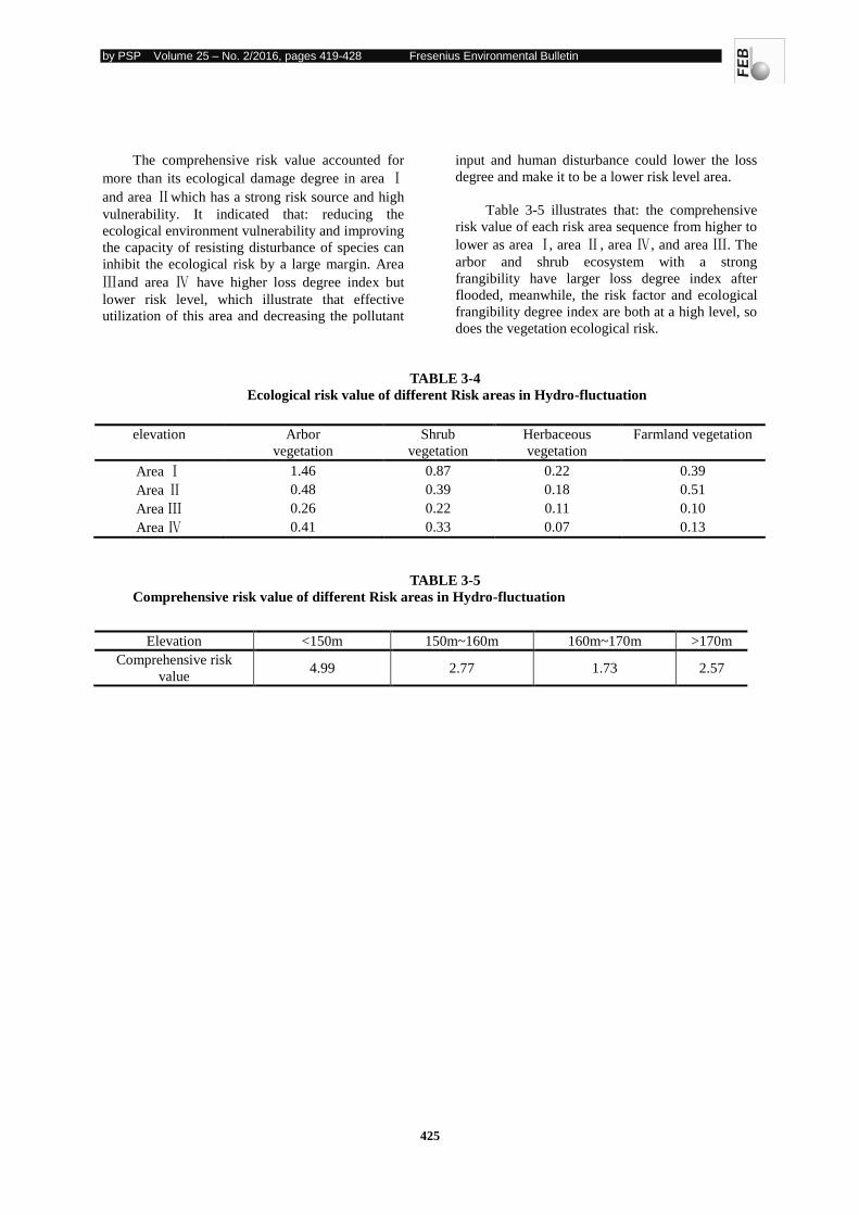
by PSP Volume 25 – No. 2/2016, pages 419-428 Fresenius Environmental Bulletin
425
The comprehensive risk value accounted for
more than its ecological damage degree in area
and area which has a strong risk source and high
vulnerability. It indicated that: reducing the
ecological environment vulnerability and improving
the capacity of resisting disturbance of species can
inhibit the ecological risk by a large margin. Area
and area have higher loss degree index but
lower risk level, which illustrate that effective
utilization of this area and decreasing the pollutant
input and human disturbance could lower the loss
degree and make it to be a lower risk level area.
Table 3-5 illustrates that: the comprehensive
risk value of each risk area sequence from higher to
lower as area , area , area , and area . The
arbor and shrub ecosystem with a strong
frangibility have larger loss degree index after
flooded, meanwhile, the risk factor and ecological
frangibility degree index are both at a high level, so
does the vegetation ecological risk.
TABLE 3-4
Ecological risk value of different Risk areas in Hydro-fluctuation
TABLE 3-5
Comprehensive risk value of different Risk areas in Hydro-fluctuation
elevation Arbor
vegetation
Shrub
vegetation
Herbaceous
vegetation
Farmland vegetation
Area 1.46 0.87 0.22 0.39
Area 0.48 0.39 0.18 0.51
Area 0.26 0.22 0.11 0.10
Area 0.41 0.33 0.07 0.13
Elevation <150m 150m~160m 160m~170m >170m
Comprehensive risk
value 4.99 2.77 1.73 2.57
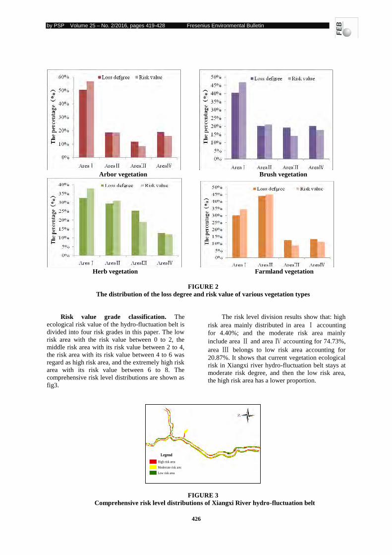
by PSP Volume 25 – No. 2/2016, pages 419-428 Fresenius Environmental Bulletin
426
Arbor vegetation Brush vegetation
Herb vegetation Farmland vegetation
FIGURE 2
The distribution of the loss degree and risk value of various vegetation types
Risk value grade classification. The
ecological risk value of the hydro-fluctuation belt is
divided into four risk grades in this paper. The low
risk area with the risk value between 0 to 2, the
middle risk area with its risk value between 2 to 4,
the risk area with its risk value between 4 to 6 was
regard as high risk area, and the extremely high risk
area with its risk value between 6 to 8. The
comprehensive risk level distributions are shown as
fig3.
The risk level division results show that: high
risk area mainly distributed in area accounting
for 4.40%; and the moderate risk area mainly
include area and area accounting for 74.73%,
area belongs to low risk area accounting for
20.87%. It shows that current vegetation ecological
risk in Xiangxi river hydro-fluctuation belt stays at
moderate risk degree, and then the low risk area,
the high risk area has a lower proportion.
FIGURE 3
Comprehensive risk level distributions of Xiangxi River hydro-fluctuation belt
Legend
High risk area
Moderrate risk area
Low risk area
by PSP Volume 25 – No. 2/2016, pages 419-428 Fresenius Environmental Bulletin
427
CONCLUSIONS
According to the above calculation and
analysis the conclusions we can drawn are as follow:
(1)Different risk areas with the same risk
source in Xiangxi river hydro-fluctuation belt have
various risk degrees, and the same risk area with
different risk sources has diverse contribution.
Areas bellow 150m and 150m~160m have larger
risk degree, its risk mainly derives from water level
and geological hazard. The risk degree is lower in
the areas above 170 m , where the soil and water
loss and human disturbance are the main risk
sources. The areas between 160 and 170m have the
lowest risk degree and its risk mainly derives from
human disturbance and geological hazard.
(2) The composition of the vegetation
ecological system with different risk areas and risk
distributions are discrepancy, which basically
shows the tendency of lower risk with the increase
of the elevation. The high vegetation ecological risk
area mostly distributed in the area bellow 150m
accounting for 4.40%, middle risk degree area
mainly lies on the area between 150m and 160m
and the area above 170m accounting for 74.73% ;and the low risk area concentrates in the area
between 160m and 170m.
(3) The current vegetation ecological risk in
Xiangxi river hydro-fluctuation belt stays at
moderate risk degree, and then the low risk area,
the high risk area has a lower proportion. The risk
grade of various vegetations are arbor vegetation,
brush vegetation, grass vegetation and farmland
vegetation by descending order.
(4) Some specific measures can be given
based on the above study. Herbaceous plants with
strong adaptability should be chosen to repair the
ecological environment which has higher flood
resistance and lower risk in area below 160m.
Meanwhile, reducing the ecological environment
vulnerability and improving the capacity of
resisting disturbance of species can inhibit the
ecological risk by a large margin. After water
storage farmland vegetation mainly distributes in
area , where Human management input reduces
the loss degree of the ecological system. So in such
area reasonable utilization of land could be a
effective measure to reduce the vegetation risk. It
also illustrates that reduction in the risk source
input and reducing of the ecological environment
vulnerability will prevent ecological risk largely.
DISCUSSIONS
And most researches on Xiangxi river pay
close attention to the water quality and vegetation
pattern changes and so on ignoring the relationship
and influence among various factors. This paper
linkes each factors by improved RRM model and
proposed appropriate indicator system. This paper
on one hand introduces anti-interference index from
the angle of vegetation ecology, on the other the
vulnerability of the environment and each
vegetation ecological system are both considered
which can reduce the inaccuracy in vulnerability
degree assessment.
The vegetation ecological risk assessment in
this paper mainly based on the changes on various
species richness and diversity of vegetation
ecosystem. So the ecological risk value mainly
reflects the impact of each risk source on the
vegetation ecosystem after the impoundment. The
assessment results in this paper can instructive
vegetation restoration and rational land use in
Xiangxi River hydro-fluctuation belt. Due to the
limitation of data the spatial distribution of
ecological risk along the Xiangxi River has not
been discussed which can be studied later.
ACKNOWLEDGEMENT
This research was supported by nation Water
Special Project for water environment risk
assessment and early warning technology research
in The three gorges reservoir area and upstream
basin(Project NO. 2013ZX07503-001). The authors
would like to thank anonymous reviewer for their
helpful comments and suggestions on corrections
and improvement of the manuscript.
REFERENCES
[1] Xu, X.G., Yan, L., Xu, L.F., Lu, Y. L. and Ma,
L.Y. (2011) Ecological Risk Assessment of
Natural Disasters in China. Acta Scientiarum
Naturalium Universitatis Pekinensis, 47(5),
901-908.
[2] Zhang, H.L. Indicators and Methods of Water
Environment Pollution Ecological Risk
Assessment in Daliao River Estuary. (2011)
Ocean University of China, 4-14.
[3] Xue, Y., Wang, R. H. and Zhang, H.Z.
Ecological Risk Assessment of Ecosystems in
the
Main stream Area of the Tarim River. (2008) Arid
zone research, 25(4), 562-567.
by PSP Volume 25 – No. 2/2016, pages 419-428 Fresenius Environmental Bulletin
428
[4] Chen, H., Li, S.C. and Zheng, D. Ecological
Risk Assessment o f Regions Alongside Qing
hai – Xizang High way and Railway Based on
Artificial Neural Network. (2005) Acta
Scientiarum Naturalium Universitatis
Pekinensis, 41(4) , 586-592.
[5] Wei, L. Study on the Ecological Vulnerability in
Shiyang River Basin Based on RS and GIS
Approach. (2010) Northwest normal
university.
[6] Sun, L., Zhou, K.F. and Jiang, L.Q. Quantitative
Assessment on Ecological Risk of Riparian
Vegetation in Arid Areas. (2008) Xinjiang
Geology, 26(1), 84-89.
[7] Dai, B.L., He, Y.L. Li, Y.Z., Chu, K.J., Xu, N.,
Wu, Z. Surface water quality assessment by
use of a combination of projection pursuit and
principal component analysis.(2014)Fresenius
Environmental Bulletin, 23(7), 1490-1496.
[8]Yang, T., Liu, J.L., Chen, Q.Y. Evaluation of
environmental flow requirement for
improvement of river ecological integrity in
the Haihe River Basin, China.(2014) Fresenius
Environmental Bulletin,23(5), 1121-1130.
[9] Zhang, S.F. and Liu, H.M. Review of ecological
risk assessment methods. (2010) Acta
Ecologica Sinica, 30 (10), 2735-2744.
[10] Xu, Y., Ma, M.H. and Gao, G. F. The
evaluation method of ecological risk
assessment based on watershed scale—Take
the Taihu watershed as example.(2012) China
Environmental Science, 32(9), 1693-1701.
[11] Xu, L.F., Xu, X.G. and Lu, Y.L. Integrated
ecological risk assessment of J-50 based on
natural disasters risk source.( 2010) Chinese
Journal of Applied Ecology, 19(11), 2607-
2612.
[12] Liu, X., Su, W.C., Wang, Z. and Huang, Y.M.
Regional ecological risk assessment of land
use in the flooding zone of the Three Gorges
Reservoir area based on relative risk
model.(2012) Acta Scientiae Circum stantiae,
32(1) , 248-256.
[13] Fu, Z.Y., Xu, X.G. and Lin, H.P. Regional
ecological risk assessment of in the Liao he
River Delta wetlands. (2001) Acta Ecologica
Sinica, 21(3), 365-373.
[14] EPA . Framework for ecological risk
assessment. (1992) Risk Assessment Forum,
EPA / 630 (1), 41.
[15] Han, X.Y., Qian, J. and Wang, L. Estimation of
soil erosion in red earth hilly area based on RS
and USLE.(2013) Remote Sensing for Land
and Resources, 25(3), 171-177.
[16] Hang, B.L. and Xue, M. Analyses of Typical
land slides in Xiangxi River Valley Affected
by Impounding.(2006) Journal of Disaster
Prevention and Mitigation Engineering, 26(3),
290-295.
[17] You, H.L., Xu, L.G., Jiang, J.H., Wang, X.L.,
Huang, Q. Liu, G.L. The effects of water level
fluctuations on the wetland landscape and
waterfowl habitat of Poyang Lake.(2014)
Fresenius Environmental Bulletin, 23(7A),
1650-1661.
[18] Xu, M., Zhang, L., Du, Y., Du, C., Zhuang,
Y.H. Adsorption characteristics of phosphorus
onto soils from different land use types in
Danjiangkou reservoir area.(2015) Fresenius
Environmental Bulletin, 24(7), 2354-2361.
[19] Li, H., Zhang, P.Y. and Cheng, Y.Q. The
concept of vulnerability and its evaluation
methods. (2008) Process of Geographical,
27(2), 18-25.
[20] Zhang, X.N. Northwest Guangxi karst region
ecological environment vulnerability. (2009)
Acta Ecologica Sinica, 29(2), 749-757.
Received: 11.06.2015
Accepted: 10.12.2015
CORRESPONDING AUTHOR
Peijiang Zhou
School of Resource and Environmental Science
Wuhan University
No. 129, Luoyu Road
430079 Wuhan – P.R. CHINA
e-mail: [email protected]
by PSP Volume 25 – No. 2/2016, pages 429-443 Fresenius Environmental Bulletin
429
EFFECTS OF SOME BOTANICAL INSECTICIDES ON THE EGG PARASITOID TRICHOGRAMMA PINTOI VOEGELÉ
(HYMENOPTERA: TRICHOGRAMMATIDAE)
Hilal Tunca1, Sahin Tatlı2, H. Hilal Moran3, Cem Özkan4
1: Ankara University, Agriculture Faculty, Department of Plant Protection, Ankara, Turkey
2: Kırıkkale University, Vocational High School, Kırıkkkale, Turkey
3: Ankara University, Agriculture Faculty, Department of Plant Protection, Ankara, Turkey
4: Ankara University, Agriculture Faculty, Department of Plant Protection, Ankara, Turkey
ABSTRACT
Egg parasitoids are among the most significant
biological control agents of a number of insect pests.
Among them, Trichogramma species are the most
widely used insect natural enemy in the world.
Generally, when it raised the idea of using biological
control, the effects of insecticides should be studied
under laboratory conditions before the release of
beneficial natural enemies. In this study, effects of
some botanical insecticides on development and
behaviour of Trichogramma pintoi Voegelé
(Hymenoptera: Trichogrammatidae) were studied. The
experiments were conducted on the host Ephestia
kuehniella Zeller (Lepidoptera: Pyralidae), at 25 ºC,
60-70% relative humidity in the laboratory condition.
In the experiments, Neem Azal (azadirachtin) and
Spruzit Neu (pyrethrum, hotpepperwax (capsaicin) and
Orange Guard (d-Limone) were tested. With the use of
LC10, LC25, LC50 ve LC90 doses of Neem Azal and
Spruzit Neu against parasitized and unparasitized E.
kuehniella eggs, insecticide side effects to the
parasitoid biology and behavior was designated.
Parasitism rate of T. pintoi was negatively affected by
application of azadirachtin and pyrethrum. This
negative effect was more observed at pyrethrum. Some
biological properties of parasitoid also showed
differences depending on parasitoid development stage,
insecticide and application dose. Emergence ratio of
the parasitoid was significantly affected by LC90 of
both insecticide. The results also showed that the most
sensitive period of parasitoid was larval stage. In adult
toxicity experiment, pyrethrum was found to be more
toxic than azadirachtin. The results of behavioral
experiments show that these botanical insecticides have
strong repellent effect to the parasitoid.
KEY WORDS: botanical insecticide, side-effect, biological control,
Trichogramma pintoi
INTRODUCTION
The use of synthetic chemical product remains a
major strategy in the pest control because it is quick,
efficient, easy to use and cost effective [1] However,
broad-spectrum insecticides are toxic to several non-
target organisms, including natural enemies. Other
negative effects of this insecticides are the
development of insecticide resistance, resurgence of
secondary pests and deleterious effects on the
environment endangering the sustainability of
agroecosystems[2]. In agroecosystem, the Ecologically
Based Integrated Pest Management (IPM) proposes the
use of environmentally respectful methods of pest
control [3] [4] [5] Insecticides of botanical origin is an
interesting way of pest control [6] [7] [8]
In this study, among botanical insecticides
azadirachtin, pyrethrum, capsaicin, d-Limonene were
used. Azadirachtin, a complex tetranortriterpenoid
limonoid from the neem seeds, cause a different of
effects in insects such as antifeedant, growth
retardation, reduced fecundity, moulting disorders,
morphogenetic defects and changes of behavior [9] [10] [11] [12].
Pyrethrum is a natural insecticide extracted from
the Composite perennial plant, Chrysanthemum
cineariaefolium, Asteraceae. The insecticide pyrethrum
contains quantities of 6 esters, collectively named
Pyretrins: Jasmolin I & II, Cinerin I & II, Pyrethrin I &
II. This insecticide is also used to control insects, such
as azadirachtin [13] .
Capsaicin is a another natural pesticide used to
repel many species of insects and mites including
aphids, lace bugs, leafhoppers, spider mites, whiteflies
by PSP Volume 25 – No. 2/2016, pages 429-443 Fresenius Environmental Bulletin
430
and thrips. Capsaicin is most effective in preventing
populations of insect pests from growing instead of
killing large infestations. It has also lethal and
antifeedant effects on different insect pests [14] [15]
Limonene (also known as d-Limonene) is produced
from citrus oils extracted from oranges and other citrus
fruit peels. it is used as an insecticide, acaricide, insect
repellent, and animal repellent [16]
These insecticides are effective againts target pest
and reputedly pose small impact to the environment [17] [18] [19]. On the other hand, the combination of
biological control and botanical insecticides, within the
concept of integrated pest management practices,
contribute to minimizing the adverse effect on the
environment [20]. One of the most studied biological
control agent, the egg parasitoids of the Trichogramma
genus (Hymenoptera: Trichogrammatidae) [21].
Parasitoids of the Trichogramma genus have important
profits as biological control agents including relative
ease of rearing and that they kill their host in the egg
stage before it causes feeding damage [22] [23]. The
minute parasitoids attacks predominately lepidopterous
hosts[24]. [25]. [26]. [27]. [28]. Trichogramma are spread
worl-wide and are successfully used large scale on
corn, cotton, sugarcane, orchard, vegetable crops and
forestry in many countries[29] [30] [31]. Also,
Trichogramma pintoi is an important parasitoid species
of lepidopterous pests in our country. The side effects
studies of synthetic insecticides and also botanical
insecticides on natural enemies is very important and
these studies have increased in the last years [4] [32] [33]
The effects of botanical insecticides were evaluated in
more than a hundred species of parasitoid and predator.
However, their biological and behavioral effects on
natural enemies may vary according to its chemical
property, formulation, dose, the natural enemy
(species, development stage vb), other environmental
factors [19]. Apart from direct toxic effects, insecticides
may prevent the feeding and foraging behavior as
repellents, inhibitors, or olfaction disruptors [34]. The
female parasitoid uses generally chemical cues to
locate a host egg. The chemical cues, called
kairomones, are on the host left near the egg by the
female during oviposition. Some of these same
chemicals are also host sex pheromones [35].These
compounds also cause interruption of sex pheromone
communication [36].
Many studies have shown that lethal effect of
insecticides on natural enemies, but sub-lethal effects
on development and behavior are overlooked.
However, studies showed that sub lethal effects can
severely decrease the quality of natural enemies [34] [37].
The objective of this study was to asses the subletal
and lethal effect of azadirachtin and Pyrethrum on
preimaginal development and their residue effect on T.
pintoi. Furthermore, the responseof the T. pintoi to
azadirachtin, pyrethrum, capsaicin, d-Limonene was
tested in air flow Y-tube olfactometer bioassays. The
result of this study may help to integrate the biological
control agents with the botanical insecticide and may
have important impact on pest control strategies in
sustainable agriculture systems.
MATERIALS AND METHODS
The host and the parasitoid. Both Ephestia
kuehniella eggs and Trichogramma pintoi were
obtained from the mass rearing unit at the Ankara
University, Faculty of Agriculture, Department Plant
Protection.
Rearing of Ephestia kuehniella. The host was
reared at 25 ± 1°C, 60-70% relative humidity (RH)
with a 16:8 h light:dark photoperiod. Culturing was
undertaken using clear plastic containers (27 x 37 x 7
cm) on a 2:1 mixture of wheat flour and rough wheat
bran containing approximately 400 g food, which was
sterilized at 60°C for 3 days, and 5.000 host eggs [38].
Rearing of Trichogramma pintoi. The parasitoid
was reared at 25±1°C and 65-75% relative humidity
with a 16:8 h light:dark photoperiod. Nearly, fresh 500
eggs (0-24 h) of E. kuehniella were glued onto cards
(5X10 cm). These cards were placed in glass tubes
(3x10cm). Newly emerged T. pintoi adults were
transferred to the glass tubes containing E. kuehniella
egg-cards and kept for 24 h.
LC Bioassays. Two botanical insectides,
azadirachtin (Neem Azal ®-T/S, Trifolio–M GMBH,
Germany-10 g/l azadirachtin) and pyrethrum (Spruzit®
Neu, Neudorff, Germany-18.36 g/l Natural-
Pyrethrum), were used. Third instar (15 days) of E.
kuehniella larvae was used for azadirachtin and
pyrethrum. LC Bioassays were conducted according to
the methods described by [37].
Effect of Ephestia kuehniella egg pre-treatement with azadirachtin and pyrethrum on Trichogramma pintoi. In the experiment, 200 0-24 h.
old aged eggs were stuck on a paper sheet (1.5 x 10
cm) with the help of 5% Arabic gum solution. LC10
LC25, LC50 and LC90 values of azadirachtin and
pyrethrum were applied on cards containing 200 E.
kuehniella eggs, using spray tower. 0, 1, 6, 12, 24 and
48 hours later the egg cards were individually place
into glass tube (3X10cm) and exposed to 15 parasitoid
females for 24 h. Parasitoids were left to mate and feed
for 24 h before host eggs were supplied. Three-five
days after exposing the parasitoids to the treated host
egg cards the number of parasitized eggs were
recorded. This experiment was replicated three times.
In the control group, only distilled water was sprayed.
by PSP Volume 25 – No. 2/2016, pages 429-443 Fresenius Environmental Bulletin
431
Side effects of Ephestia kuehniella egg post treatement with azadirachtin and pyrethrum on Trichogramma pintoi. Ephestia kuehniella eggs were
used to investigate the effects of azadirachtin and
pyrethrum on preimaginal stages of T. pintoi
developing within the host eggs. 30 0-24 h. old aged
eggs were stuck on a paper sheet (1.5 x 10 cm) with the
help of 5% Arabic gum solution. Egg cards containing
30 E. kuehniella eggs were offered to two T. pintoi females for 24 h. Parasitoids were left to mate and feed
for 24 h before host eggs were supplied. Egg cards
were removed and 72 hours, 144 hours and 192 hours
later. These days correspond to larval, prepupal and
pupal stages of Trichogramma, respectively [39] [40] [41].
After these egg cards were sprayed either with LC10,
LC25, LC50 and LC90 values of azadirachtin and
pyrethrum. The treated egg cards were allowed to dry
for 20 minute. In the control group, only distilled water
was sprayed. Each egg card was then transferred to a
glass tube (3x10 cm) and placed rearing room (25±1°C
and 65-75% relative humidity, with a 16:8 h light:dark
photoperiod) and checked daily till the emergence of
adult parasitoids to determine the tested biological
parameters (emergence ratio, development time and
longevity). Longevities of the parasitoid were
investigated at two different condition (with food-
honey and without food). This experiment was
replicated three times.
Side effects of azadirachtin and pyrethrum on Trichogramma pintoi adult. In order to determine
initial toxicity, the adult T. pintoi was exposed to a
fresh dry pesticide film applied on glass plates at the
LC10 LC25, LC50 and LC90 values of azadirachtin and
pyrethrum. The exposure cage contained in two square
glass plates and an aleminium frame (13cm long, 1.5
cm high, and 1cm wide). Each of three sides of the
frame contained six ventilation holes (1cm diameter),
covered with black tight material [30] The glass plates
coated with 2 + 0.2 mg/cm2 of LC10 LC25, LC50 and
LC90 values of azadirachtin and pyrethrum with the use
of spray tower and allowed to dry for 30 minute. T.
pintoi adults were introduced into the exposure cages
by emergence tubes. The number of dead wasps in each
glass plate was counted 24 h after initial exposure to
azadirachtin and pyrethrum residue in glass plates.
Data were corrected for mortality in the controls using
Abbott’s formula [42]. Each treatement was replicated 4
times. At the end of 24 h exposure, the parasitoids, if
still alive, were given host eggs to measure their
capacity of parasitism. Fifteen eggs of E. kuehniella
were offered to one female parasitoid. A female
parasitoid was removed after 24 h. The capacity of
parasitism per T. pintoi female and the reduction in
capacity compared with the control was used to
measure the effect of insecticide.
Olfactory bioassays. Olfactometric assays were
conducted according to the methods described by [43].
In the experiment, Naive, mated and fed female
parasitoids (0-24 hours old) were introduced singly into
the stem of the olfactometer. In choice testing, the
behavioural response of T. pintoi to azadirachtin (LC10,
LC50 and LC90),pyrethrum (LC10, LC50 and LC90),
capsaicin (1:32) (Hotpepperwax) and d-Limonene (1:4)
(Orange guard), and clean air, was assessed in a Y-
olfactometer. Experiments were carrying out three
times and each replicate involved 10 adult parasitoids.
All tests were conducted at 25±1, 65–75% RH. Choice
test was carried out by the following treatments: (1)
Insecticide-a clean air; (2) Insecticide + host egg-a
clean air (3) distile water- clean air (control).
Statistical analysis. Dose–response bioassay data
for LC10, LC25, LC50, LC90 determinations were
analyzed with the probit procedure [44]. Differences
were considered significant when 95% fiducial limits
(FL) did not overlap. Emergence, longevity and
reproduction data were analyzed with one-way
analyses of variance (ANOVA). Percentage data were
arcsine transformed before analysis. In olfactometric
assays, data were analysed using the Z test.
RESULTS AND DISCUSSION
Using multiple dose assays with azadirachtin and
pyrethrum, different LC10, LC25, LC50 and LC90 values
for the third developmental stages of E. kuehniella was
determined. LC50 of azadirachtin to E. kuehniella
ranged from 409.3-722.6. LC50 of pyrethrum to E.
kuehniella ranged from 63.5-111.3 (Table 1).
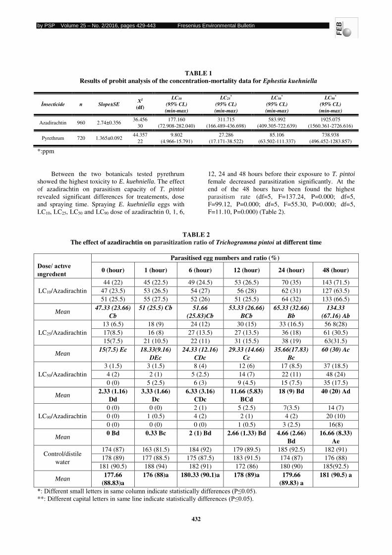
by PSP Volume 25 – No. 2/2016, pages 429-443 Fresenius Environmental Bulletin
432
TABLE 1 Results of probit analysis of the concentration-mortality data for Ephestia kuehniella
İnsecticide n Slope±SE Χ2
(df)
LC10
(95% CL)
(min-max)
LC25*
(95% CL)
(min-max)
LC50*
(95% CL)
(min-max)
LC90*
(95% CL)
(min-max)
Azadirachtin 960 2.74±0.356 36.456
30
177.160
(72.908-282.040)
311.715
(166.489-436.698)
583.992
(409.305-722.639)
1925.075
(1560.361-2726.616)
Pyrethrum 720 1.365±0.092 44.357
22
9.802
(4.966-15.791)
27.286
(17.171-38.522)
85.106
(63.502-111.337)
738.938
(496.452-1283.857)
*:ppm
Between the two botanicals tested pyrethrum
showed the highest toxicity to E. kuehniella. The effect
of azadirachtin on parasitism capacity of T. pintoi
revealed significant differences for treatements, dose
and spraying time. Spraying E. kuehniella eggs with
LC10, LC25, LC50 and LC90 dose of azadirachtin 0, 1, 6,
12, 24 and 48 hours before their exposure to T. pintoi
female decreased parasitization significantly. At the
end of the 48 hours have been found the highest
parasitism rate (df=5, F=137.24, P=0.000; df=5,
F=99.12, P=0.000; df=5, F=55.30, P=0.000; df=5,
F=11.10, P=0.000) (Table 2).
TABLE 2 The effect of azadirachtin on parasitization ratio of Trichogramma pintoi at different time
Dose/ actıve ıngredıent
Parasitised egg numbers and ratio (%)
0 (hour) 1 (hour) 6 (hour) 12 (hour) 24 (hour) 48 (hour)
LC10/Azadirachtin
44 (22) 45 (22.5) 49 (24.5) 53 (26.5) 70 (35) 143 (71.5)
47 (23.5) 53 (26.5) 54 (27) 56 (28) 62 (31) 127 (63.5)
51 (25.5) 55 (27.5) 52 (26) 51 (25.5) 64 (32) 133 (66.5)
Mean 47.33 (23.66)
Cb
51 (25.5) Cb 51.66
(25.83)Cb
53.33 (26.66)
BCb
65.33 (32.66)
Bb
134.33
(67.16) Ab
LC25/Azadirachtin
13 (6.5) 18 (9) 24 (12) 30 (15) 33 (16.5) 56 8(28)
17(8.5) 16 (8) 27 (13.5) 27 (13.5) 36 (18) 61 (30.5)
15(7.5) 21 (10.5) 22 (11) 31 (15.5) 38 (19) 63(31.5)
Mean 15(7.5) Ec 18.33(9.16)
DEc
24.33 (12.16)
CDc
29.33 (14.66)
Cc
35.66(17.83)
Bc
60 (30) Ac
LC50/Azadirachtin
3 (1.5) 3 (1.5) 8 (4) 12 (6) 17 (8.5) 37 (18.5)
4 (2) 2 (1) 5 (2.5) 14 (7) 22 (11) 48 (24)
0 (0) 5 (2.5) 6 (3) 9 (4.5) 15 (7.5) 35 (17.5)
Mean 2.33 (1.16)
Dd 3.33 (1.66)
Dc 6.33 (3.16)
CDc 11.66 (5.83)
BCd 18 (9) Bd 40 (20) Ad
LC90/Azadirachtin
0 (0) 0 (0) 2 (1) 5 (2.5) 7(3.5) 14 (7)
0 (0) 1 (0.5) 4 (2) 2 (1) 4 (2) 20 (10)
0 (0) 0 (0) 0 (0) 1 (0.5) 3 (2.5) 16(8)
Mean 0 Bd 0.33 Bc 2 (1) Bd 2.66 (1.33) Bd 4.66 (2.66)
Bd 16.66 (8.33)
Ae
Control/distile
water
174 (87) 163 (81.5) 184 (92) 179 (89.5) 185 (92.5) 182 (91)
178 (89) 177 (88.5) 175 (87.5) 183 (91.5) 174 (87) 176 (88)
181 (90.5) 188 (94) 182 (91) 172 (86) 180 (90) 185(92.5)
Mean 177.66
(88.83)a 176 (88)a 180.33 (90.1)a 178 (89)a 179.66
(89.83) a 181 (90.5) a
*: Different small letters in same column indicate statistically differences (P≤0.05). **: Different capital letters in same line indicate statistically differences (P≤0.05).
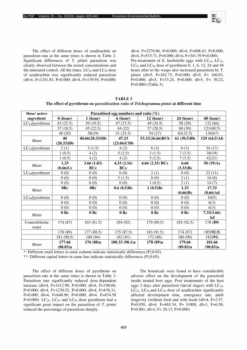
by PSP Volume 25 – No. 2/2016, pages 429-443 Fresenius Environmental Bulletin
433
The effect of different doses of azadirachtin on
parasitism rate at the same times is shown in Table 2.
Significant differences of T. pintoi parasitism was
clearly observed between the tested concentrations and
the untreated control. All the times, LC50 and LC90 dose
of azadirachtin was significantly reduced parasitism
(df=4, F=1241.83, P=0.000; df=4, F=139.93, P=0.000;
df=4, F=2276.06, P=0.000; df=4, F=608.43, P=0.000;
df=4, F=515.71, P=0.000; df=4, F=341.39 P=0.000).
Pre-treatement of E. kuehniella eggs with LC10, LC25,
LC50 and LC90 dose of pyrethrum 0, 1, 6, 12, 24 and 48
hours after to the wasps also increased parasitism by T.
pintoi (df=5, F=162.73, P=0.000; df=5, F= 166.03,
P=0.000; df=5, F=33.24, P=0.000; df=5, F= 30.22,
P=0.000) (Table 3).
TABLE 3 The effect of pyrethrum on parasitization ratio of Trichogramma pintoi at different time
Dose/ actıve ıngredıent
Parasitised egg numbers and ratio (%) 0 (hour) 1 (hour) 6 (hour) 12 (hour) 24 (hour) 48 (hour)
LC10/pyrethrum 43 (22.5) 39 (19.5) 47 (23.5) 49 (24.5) 58 (29) 132 (66)
37 (18.5) 45 (22.5) 44 (22) 57 (28.5) 60 (30) 121(60.5)
40 (20) 38(19) 51 (25.5) 54 (27) 65(32.5) 134(67)
Mean 40
(20.33)Db 40.66(20.33)Db 47.33
(23.66)CDb 53.33(26.66)BCb 61 (30.5)Bb 129 (64.5)Ab
LC25/pyrethrum 2 (1) 3 (1.5) 4 (2) 6 (3) 6 (3) 34 (17)
1 (0.5) 4 (2) 5 (2.5) 3 (1.5) 7 (3.5) 38(19)
1 (0.5) 4 (2) 4 (2) 5 (2.5) 7 (3.5) 42(21)
Mean 1.33
(0.66)Cc 3.66 (1.83)
BCc 4.33 (2.16)
BCc 4.66 (2.33) BCc 6.66
(3.33)Bc 38 (19)Ac
LC50/pyrethrum 0 (0) 0 (0) 0 (0) 2 (1) 0 (0) 22 (11)
0 (0) 0 (0) 3 (1.5) 0 (0) 2 (1) 16 (8)
0 (0) 0 (0) 0 (0) 1 (0.5) 2 (1) 14 (7)
Mean 0Bc 0Bc 0.6 (0.5)Bc 1 (0.5)Bc 1.33
(0.66)Bc 17.33
(8.66)Ad LC90/pyrethrum 0 (0) 0 (0) 0 (0) 0 (0) 0 (0) 10(5)
0 (0) 0 (0) 0 (0) 0 (0) 0 (0) 6(3)
0 (0) 0 (0) 0 (0) 0 (0) 0 (0) 6(3)
Mean 0 Bc 0 Bc 0 Bc 0 Bc 0 Bc 7.33(3.66)
Ad Control/distile
water
174 (87) 163 (81.5) 184 (92) 179 (89.5) 185 (92.5) 178 (89)
178 (89) 177 (88.5) 175 (87.5) 183 (91.5) 174 (87) 185(92.5) 181 (90.5) 188 (94) 182 (91) 172 (86) 180 (90) 182(91)
Mean 177.66
(88.83)a 176 (88)a 180.33 (90.1)a 178 (89)a 179.66
(89.83)a 181.66
(90.83)a *: Different small letters in same column indicate statistically differences (P≤0.05). **: Different capital letters in same line indicate statistically differences (P≤0.05).
The effect of different doses of pyrethrum on
parasitism rate at the same times is shown in Table 3.
Parasitism rate significantly reduced dose-dependent
increase (df=4, F=1412.90, P=0.000; df=4, F=190.60,
P=0.000; df=4, F=1230.52, P=0.000; df=4, F=676.31,
P=0.000; df=4, F=640.96, P=0.000; df=4, F=674.58
P=0.000). LC25, LC50 and LC90 dose pyrethrum had a
significant great impact on the parasitism of T. pintoi
reduced the percentage of parasitism sharply.
The botanicals were found to have considerable
adverse effect on the development of the parasitoid
inside treated host eggs. Post treatements of the host
eggs 3 days after parasitism (larval stages) with LC10,
LC25, LC50 and LC90 dose of azadirachtin significantly
affected development time, emergence rate, adult
longevity (without food and with food) (df=4, F=2.57,
P=0.039, df=4, F=465.34, P= 0.000, df=3, F=6.50,
P=0.001; df=3, F= 20.13, P=0.000).
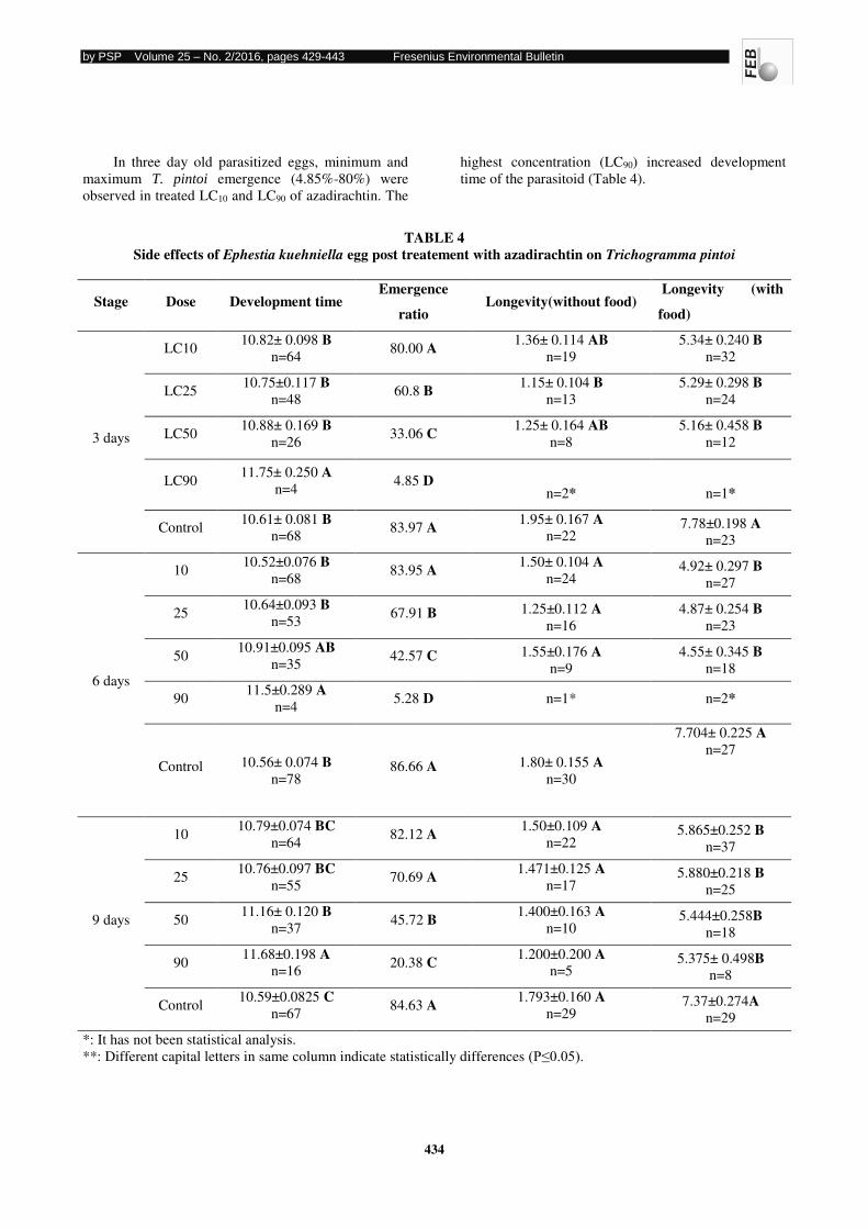
by PSP Volume 25 – No. 2/2016, pages 429-443 Fresenius Environmental Bulletin
434
In three day old parasitized eggs, minimum and
maximum T. pintoi emergence (4.85%-80%) were
observed in treated LC10 and LC90 of azadirachtin. The
highest concentration (LC90) increased development
time of the parasitoid (Table 4).
TABLE 4 Side effects of Ephestia kuehniella egg post treatement with azadirachtin on Trichogramma pintoi
Stage Dose Development time Emergence
ratio Longevity(without food)
Longevity (with
food)
3 days
LC10 10.82± 0.098 B
n=64 80.00 A
1.36± 0.114 AB
n=19
5.34± 0.240 B
n=32
LC25 10.75±0.117 B
n=48 60.8 B
1.15± 0.104 B
n=13
5.29± 0.298 B
n=24
LC50 10.88± 0.169 B
n=26 33.06 C
1.25± 0.164 AB
n=8
5.16± 0.458 B
n=12
LC90 11.75± 0.250 A
n=4 4.85 D
n=2*
n=1*
Control 10.61± 0.081 B
n=68 83.97 A
1.95± 0.167 A
n=22 7.78±0.198 A
n=23
6 days
10 10.52±0.076 B
n=68 83.95 A
1.50± 0.104 A
n=24 4.92± 0.297 B
n=27
25 10.64±0.093 B
n=53 67.91 B 1.25±0.112 A
n=16
4.87± 0.254 B
n=23
50 10.91±0.095 AB
n=35 42.57 C 1.55±0.176 A
n=9
4.55± 0.345 B
n=18
90 11.5±0.289 A
n=4 5.28 D n=1* n=2*
Control 10.56± 0.074 B
n=78 86.66 A 1.80± 0.155 A
n=30
7.704± 0.225 A
n=27
9 days
10 10.79±0.074 BC
n=64 82.12 A
1.50±0.109 A
n=22 5.865±0.252 B
n=37
25 10.76±0.097 BC
n=55 70.69 A
1.471±0.125 A
n=17 5.880±0.218 B
n=25
50 11.16± 0.120 B
n=37 45.72 B
1.400±0.163 A
n=10 5.444±0.258B
n=18
90 11.68±0.198 A
n=16 20.38 C
1.200±0.200 A
n=5 5.375± 0.498B
n=8
Control 10.59±0.0825 C
n=67 84.63 A
1.793±0.160 A
n=29 7.37±0.274A
n=29
*: It has not been statistical analysis.
**: Different capital letters in same column indicate statistically differences (P≤0.05).
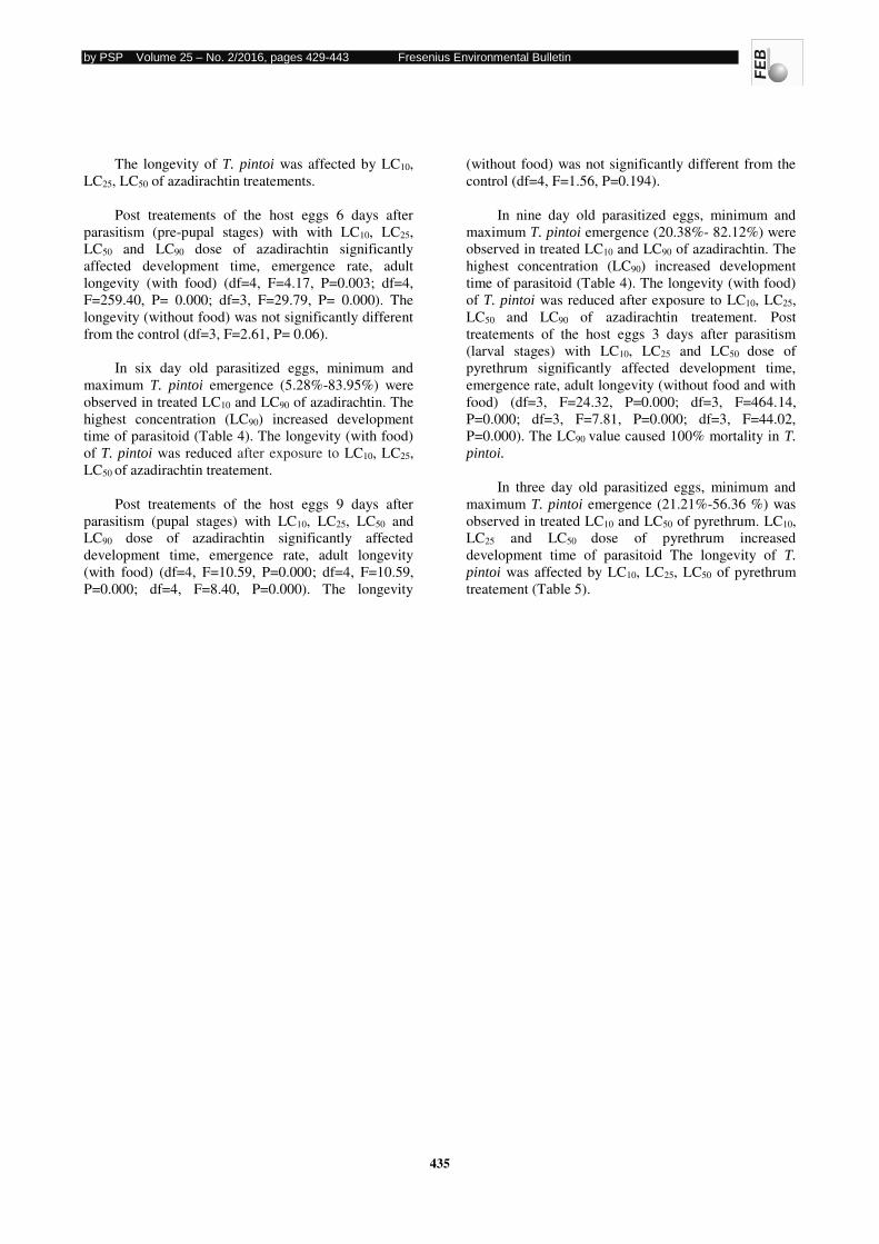
by PSP Volume 25 – No. 2/2016, pages 429-443 Fresenius Environmental Bulletin
435
The longevity of T. pintoi was affected by LC10,
LC25, LC50 of azadirachtin treatements.
Post treatements of the host eggs 6 days after
parasitism (pre-pupal stages) with with LC10, LC25,
LC50 and LC90 dose of azadirachtin significantly
affected development time, emergence rate, adult
longevity (with food) (df=4, F=4.17, P=0.003; df=4,
F=259.40, P= 0.000; df=3, F=29.79, P= 0.000). The
longevity (without food) was not significantly different
from the control (df=3, F=2.61, P= 0.06).
In six day old parasitized eggs, minimum and
maximum T. pintoi emergence (5.28%-83.95%) were
observed in treated LC10 and LC90 of azadirachtin. The
highest concentration (LC90) increased development
time of parasitoid (Table 4). The longevity (with food)
of T. pintoi was reduced after exposure to LC10, LC25,
LC50 of azadirachtin treatement.
Post treatements of the host eggs 9 days after
parasitism (pupal stages) with LC10, LC25, LC50 and
LC90 dose of azadirachtin significantly affected
development time, emergence rate, adult longevity
(with food) (df=4, F=10.59, P=0.000; df=4, F=10.59,
P=0.000; df=4, F=8.40, P=0.000). The longevity
(without food) was not significantly different from the
control (df=4, F=1.56, P=0.194).
In nine day old parasitized eggs, minimum and
maximum T. pintoi emergence (20.38%- 82.12%) were
observed in treated LC10 and LC90 of azadirachtin. The
highest concentration (LC90) increased development
time of parasitoid (Table 4). The longevity (with food)
of T. pintoi was reduced after exposure to LC10, LC25,
LC50 and LC90 of azadirachtin treatement. Post
treatements of the host eggs 3 days after parasitism
(larval stages) with LC10, LC25 and LC50 dose of
pyrethrum significantly affected development time,
emergence rate, adult longevity (without food and with
food) (df=3, F=24.32, P=0.000; df=3, F=464.14,
P=0.000; df=3, F=7.81, P=0.000; df=3, F=44.02,
P=0.000). The LC90 value caused 100% mortality in T.
pintoi.
In three day old parasitized eggs, minimum and
maximum T. pintoi emergence (21.21%-56.36 %) was
observed in treated LC10 and LC50 of pyrethrum. LC10,
LC25 and LC50 dose of pyrethrum increased
development time of parasitoid The longevity of T.
pintoi was affected by LC10, LC25, LC50 of pyrethrum
treatement (Table 5).
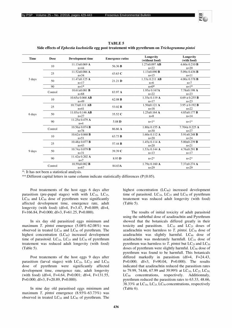
by PSP Volume 25 – No. 2/2016, pages 429-443 Fresenius Environmental Bulletin
436
TABLE 5 Side effects of Ephestia kuehniella egg post treatement with pyrethrum on Trichogramma pintoi
Time Dose Development time Emergence ratioı Longevity (without food)
Longevity (with food)
3 days
10 11.13±0.069 A
n=44 56.36 B
1.27±0.097 AB
n=22
4.60± 0.210 B
n=20
25 11.52±0.086 A
n=34 43.63 C
1.13±0.090 B
n=15
5.09± 0.436 B
n=11
50 11.47±0.125 A
n=17 21.21 D
1.33± 0.211 AB
n=6
4.00± 0.378 B
n=7
90 n=1* n=0* n=1*
Control 10.61±0.081 B
n=68 83.97 A
1.95± 0.167A
n=22
7.78±0.198 A
n=23
6 days
10 10.65± 0.068 AB
n=49 62.08 B
1.35± 0.119 A
n=17
4.69 ± 0.255 B
n=23
25 10.73±0.111 AB
n=41 53.02 B
1.50±0.121 A
n=18
3.95 ± 0.192 B
n=22
50 11.03± 0.146 AB
n=27 35.52 C
1.25±0.164 A
n=8
4.85±0.177 B
n=14
90 11.25± 0.479 A
n=4 5.08 D n=1* n=1*
Control 10.56± 0.074 B
n=78 86.66 A
1.80± 0.155 A
n=30
7.704± 0.225 A
n=27
9 days
10 10.62± 0.068 B
n=51 63.73 B
1.60± 0.112 A
n=20
5.91±0.248 B
n=24
25 10.48± 0.077 B
n=43 57.44 B
1.45± 0.114 A
n=20
5.00±0.239 B
n=21
50 10.74± 0.079 B
n=31 39.39 C
1.53± 0.144 A
n=13
4.76±0.291 B
n=17
90 11.42± 0.202 A
n=7 8.93 D n=2* n=2*
Control 10.59±0.082 B
n=67 84.63A
1.79± 0.160 A
n=29
7.37±0.274 A
n=29
*: It has not been a statistical analysis.
**:Different capital letters in same column indicate statistically differences (P≤0.05).
Post treatements of the host eggs 6 days after
parasitism (pre-pupal stages) with with LC10, LC25,
LC50 and LC90 dose of pyrethrum were significantly
affected development time, emergence rate, adult
longevity (with food) (df=4, F=3.47, P=0.009; df=4,
F=166.84, P=0.000; df=3, F=61.25, P=0.000).
In six day old parasitized eggs minimum and
maximum T. pintoi emergence (5.08%-62.08%) was
observed in treated LC10 and LC90 of pyrethrum. The
highest concentration (LC90) increased development
time of parasitoid. LC10, LC25 and LC50 of pyrethrum
treatement was reduced adult longevity (with food)
(Table 5).
Post treatements of the host eggs 9 days after
parasitism (larval stages) with LC10, LC25 and LC50
dose of pyrethrum were significantly affected
development time, emergence rate, adult longevity
(with food) (df=4, F=4.64, P=0.001; df=4, F=131.55,
P=0.000; df=3, F=20.89, P=0.000).
In nine day old parasitised eggs minimum and
maximum T. pintoi emergence (8.93%-63.73%) was
observed in treated LC10 and LC90 of pyrethrum. The
highest concentration (LC90) increased development
time of parasitoid. LC10, LC25 and LC50 of pyrethrum
treatement was reduced adult longevity (with food)
(Table 5).
The results of initial toxicity of adult parasitoid
using the sublethal dose of azadirachtin and Pyrethrum
showed that the botanicals differed greatly in their
toxicity and parasitism. LC10 and LC25 doses of
azadirachtin were harmless to T. pintoi. LC50 dose of
azadirachtin was slightly harmful. LC90 dose of
azadirachtin was moderately harmfull. LC10 dose of
pyrethrum was harmless to T. pintoi but LC25 and LC50
doses of pyrethrum were slightly harmful. LC90 dose of
pyrethrum was found to be harmfull. This botanicals
differed markedly in parasitism (df=4, F=24.43,
P=0.000; df=3, F=90.04, P=0.000). The results
indicated that azadirachtin reduced the parasitism rates
to 79.99, 74.66, 67.99 and 39.99% at LC10, LC25, LC50,
LC90 concentrations, respectively. Additionnaly,
pyrethrum reduced the parasitism rates to 63.33, 48.66,
38.33% at LC10, LC25, LC50 concentrations, respectively
(Table 6).
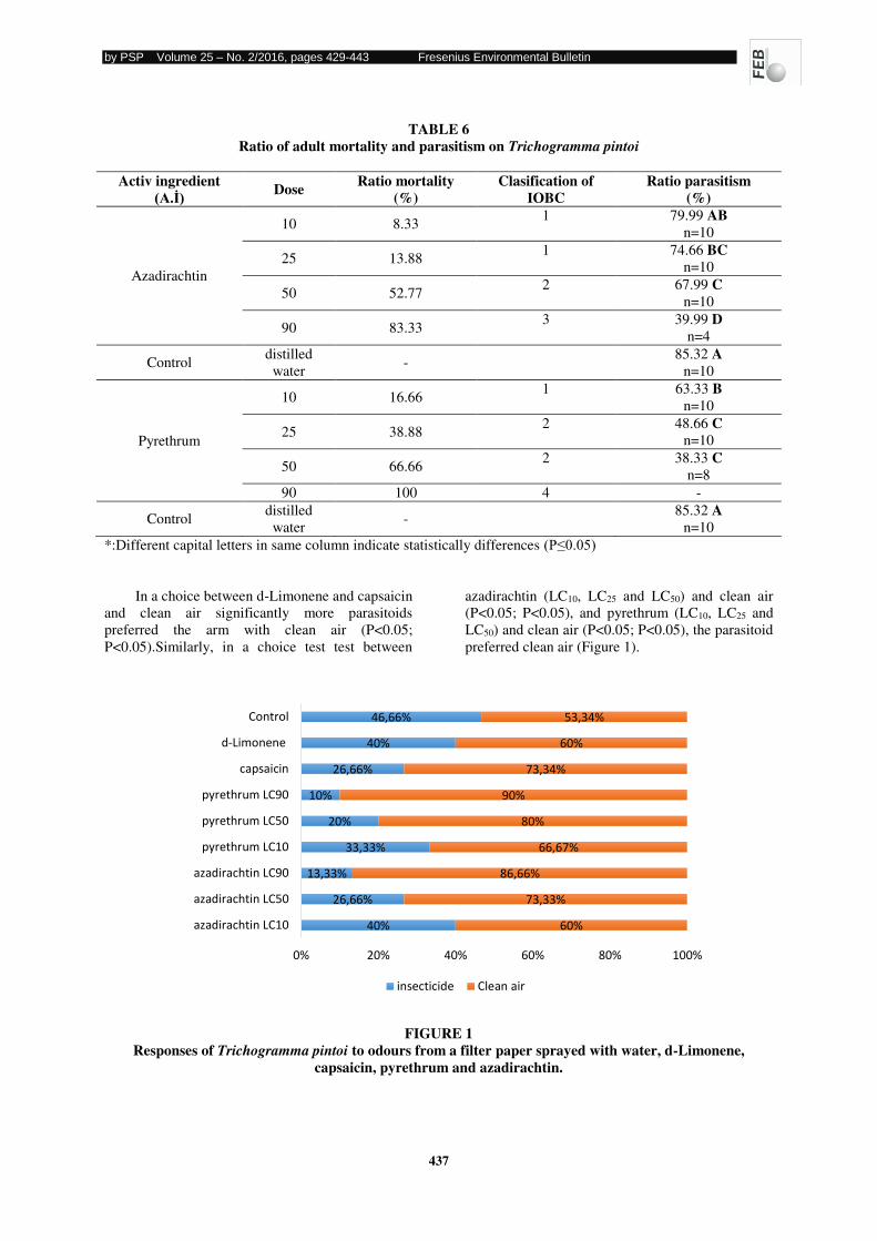
by PSP Volume 25 – No. 2/2016, pages 429-443 Fresenius Environmental Bulletin
437
TABLE 6 Ratio of adult mortality and parasitism on Trichogramma pintoi
Activ ingredient (A.İ) Dose
Ratio mortality (%)
Clasification of IOBC
Ratio parasitism (%)
Azadirachtin
10 8.33 1 79.99 AB
n=10
25 13.88 1 74.66 BC
n=10
50 52.77 2 67.99 C
n=10
90 83.33 3 39.99 D
n=4
Control distilled
water -
85.32 A n=10
Pyrethrum
10 16.66 1 63.33 B
n=10
25 38.88 2 48.66 C
n=10
50 66.66 2 38.33 C
n=8
90 100 4 -
Control distilled
water -
85.32 A
n=10
*:Different capital letters in same column indicate statistically differences (P≤0.05)
In a choice between d-Limonene and capsaicin
and clean air significantly more parasitoids
preferred the arm with clean air (P<0.05;
P<0.05).Similarly, in a choice test test between
azadirachtin (LC10, LC25 and LC50) and clean air
(P<0.05; P<0.05), and pyrethrum (LC10, LC25 and
LC50) and clean air (P<0.05; P<0.05), the parasitoid
preferred clean air (Figure 1).
FIGURE 1 Responses of Trichogramma pintoi to odours from a filter paper sprayed with water, d-Limonene,
capsaicin, pyrethrum and azadirachtin.
40%
26,66%
13,33%
33,33%
20%
10%
26,66%
40%
46,66%
60%
73,33%
86,66%
66,67%
80%
90%
73,34%
60%
53,34%
0% 20% 40% 60% 80% 100%
azadirachtin LC10
azadirachtin LC50
azadirachtin LC90
pyrethrum LC10
pyrethrum LC50
pyrethrum LC90
capsaicin
d-Limonene
Control
insecticide Clean air
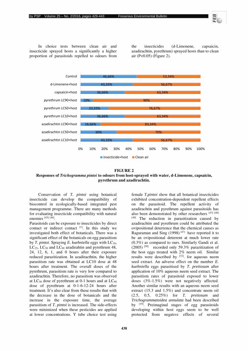
by PSP Volume 25 – No. 2/2016, pages 429-443 Fresenius Environmental Bulletin
438
In choice tests between clean air and
insecticide sprayed hosts a significantly a higher
proportion of parasitoids repelled to odours from
the insecticides (d-Limonene, capsaicin,
azadirachtin, pyrethrum) sprayed hosts than to clean
air (P<0.05) (Figure 2).
FIGURE 2 Responses of Trichogramma pintoi to odours from host-sprayed with water, d-Limonene, capsaicin,
pyrethrum and azadirachtin.
Conservation of T. pintoi using botanical
insecticide can develop the compatibility of
biocontrol in ecologically-based integrated pest
management programme. There are many methods
for evaluating insecticide compatibility with natural
enemies [45] [46].
Parasitoids can be exposure to insecticides by direct
contact or indirect contact [1]. In this study we
investigated both effect of botanicals. There was a
significant effect of the botanicals on egg parasitism
by T. pintoi. Spraying E. kuehniella eggs with LC10,
LC25, LC50 and LC90 azadirahtin and pyrethrum 48,
24, 12, 6, 1, and 0 hours after their exposure
reduced parazitization. In azadiracthtin, the higher
parasitism rate was obtained at LC10 dose at 48
hours after treatment. The overall doses of the
pyrethrum, parasitism rate is very low compared to
azadirachtin. Therefore, no parasitism was observed
at LC50 dose of pyrethrum at 0-1 hours and at LC90
dose of pyrethrum at 0-1-6-12-24 hours after
treatment. İt’s also clear from these results that with the decrease in the dose of botanicals and the
increase in the exposure time, the average
parasitism of T. pintoi is increased. The side-effects
were minimized when these pesticides are applied
at lower concentrations. Y tube choice test using
female T.pintoi show that all botanical insecticides
exhibited concentration-dependent repellent effects
on the parasitoid. The repellent activity of
azadirachtin and pyrethrum against parasitoids has
also been demonstrated by other researchers [47] [48]
[49] The reduction in parasitization caused by
azadirachtin and pyrethrum could be attributed the
ovipositional deterrence that the chemical causes as
Raguraman and Sing (1998) [47] have reported it to
be an ovipositional deterrent at much lower rate
(0.3%) as compared to ours. Similarly Gandi et al.
(2005) [50] recorded only 59.3% parazitization of
the host eggs treated with 2% neem oil. Similar
results were described by [32]. for aqueous neem
seed extract. An adverse effect on the number E.
kuehniella eggs parasitised by T. pretiosum after
application of 10% aqueous neem seed extract. The
parasitism rates of parasitoid exposed to lower
doses (3%-1.5%) were not negatively affected.
Another similar results with an aqueous neem seed
extract (15.3 and 1.5%) and concentrate neem oil
(2.5, 0.5, 0.25%) for T. pretiosum and
Trichogrammatoidea annulata had been described
by [19]. Preimaginal stages of egg parasitoids
developing within host eggs seem to be well
protected from negatıve effects of several
43,33%
30%
16,66%
36,66%
23,33%
10%
36,66%
43,33%
46,66%
56,67%
70%
83,34%
63,34%
76,67%
90%
63,34%
56,67%
53,34%
0% 10% 20% 30% 40% 50% 60% 70% 80% 90% 100%
azadirachtin LC10+host
azadirachtin LC50+host
azadirachtin LC90+host
pyrethrum LC10+host
pyrethrum LC50+host
pyrethrum LC90+host
capsaicin+host
d-Limonene+host
Control
insecticide+host Clean air
by PSP Volume 25 – No. 2/2016, pages 429-443 Fresenius Environmental Bulletin
439
insecticides. Because the egg chorion is a kind of
protection to developmental stages [39] [51] [52] [53].
However, the toxic effect of insecticides might
depend on product formulation, concentration, the
progression of preimaginal development at time of
exposure, host egg and on Trichogramma species [19]. Orr et al. (1989) [52] reported that the
developmental stage of parasitoids at the time of
insecticide treatment is important because it detects
the times permited for insecticide degradation
before emergence of parasitoids. However, the host
egg plays an important role on the effect of
insecticide on preimagınal stages. Insecticides can pass or not pass from the chorion depend on host
egg [54] [55]. Hence, this situation affects disruptive
effect level. Saber et al. (2004) [55] reported that
azadirachtin could penetrate the host’s egg chorion to some extent and made the adult parasitoids
unable to emerge and also pyrethrum. In current
study, the timing of the insecticide treatement
relative to three preimaginal development stages
had significant effect on emergence. When T. pintoi
preimaginal stages developing within E. kuehniella
eggs were exposed to the insecticides larval and
prepupal stages resulted in lower emergence than
pupal stage. The disruptive effect of azadirachtin
and pyrethrum on T. pintoi emergence decreased as
the parasitoid advanced in development, and the
pupal stage had the hıghest emergence rate. Similar observations were made by [41] who examined
spinosad effects on egg parasitoid T.exiguum early
developmental stages and reported that the
emergence ratio increased while preimaginal
development advanced. [53] showed that the most
susceptible stage was found as larvae while treated
with spinosad T. evanescens and T. bourarachaev,
however for T.cacoeciae this phenomon was higher
for prepupae stages. Hohmann et al. (2010) [19]
reported that the susceptibility of the T. pretiosum
pre-imaginal stage varies its developmental stage
and neem formulation. The egg-first larval instar
was the most influenced, stage when aqueous neem
seed extract was used, whereas emulsifiable
concentrate neem oil was more destructive to
prepupal stage. Another report by [56] who tested
side effects of 21 pesticides on the hymenoptera
egg parasitoid T. cacoeciae, they reported that the
pyrethrum was harmfulll the adult parasitoid and
pupal stage within host egg. Sattar et al. (2011) [57]
showed that degrees of toxicity for the insecticides
used againts the different immature stages of T.
chilonis inside host eggs. Six insecticides were
tested against all the life stage of parasitoid. Neem
oil was harmless to the eggs, pupae, and adults but
exerted slightly harmful effects on larval
development and female fecundity.
In addition, post-treatements of the host eggs
with azadirachtin and pyrethrum reduced T. pintoi
survival. Hohmann et al. (2010) [19] were treated
host eggs with emulsifiable concentrate neem oil
(ECNO) at concentrations varying from 2.5% to
0.25% did not affect T. pretiosum longevity, but the
highest concentration (2.5%) reduced T.annulata
survival. Oliveira et al. (2003) [58] however reported
significant reduction on longevity of T. pretiosum
on A. kuehniella eggs even concentrations variying
from 1.25% to 2% were tested.
Concerning the insecticide effects on
Trichogramma adult, azadirachtin and pyrethrum
residues were changed depend on dose. But LC90
dose of azadirachtin and pyrethrum were found to
be very toxic. In addition, the results demonstrated
that the percentage of parasitism of T. pintoi was
significantly reduced compared with control after
insecticide residue application. Abdelgader (2012)
[59] reported that residues of Neem Azal
formulations on glass plates were either harmfull
(Neem Azal-Blank) or moderately harmful
(Celaflor) T. cacoeciae adults.
CONCLUSIONS
No literature is available on the effects of
insecticide on T. pintoi, except this study. The
combination different methods used in the present
work to test the effect of botanicals on T. pintoi
showed that usefull information to evaluate on the
total effect of this chemicals. The results showed
that, in general, that high dose of azadirachtin and
pyrethrum weren’t relatively safe to tested parasitoid. Also four botanicals have a strong
repellent effect against T. pintoi.
Nevertheless, it is crucial to advert, that this
research was accomplished under controlled
conditions where the wasp was submitted to the
highest possible insecticide pressure, then field crop
conditions insecticides might have their toxic effect
decreased becaused the natural enemies can benefit
from natural refuges or avoid treated areas.
Furthermore, sunlight degration contribute to
reduce the effect of insecticides on the biological
control agents observed in laboratory [60]
ACKNOWLEDGEMENTS
This study was supported by the Scientific and
Technological Research Council of Turkey.
by PSP Volume 25 – No. 2/2016, pages 429-443 Fresenius Environmental Bulletin
440
REFERENCES
[1] Wang, H.Y., Yang, Y., Su, J.Y., Shen, J.L.,
Gao, C.F. and Zhu, Y.C. 2008. Assessment of
the impact of insecticides on Anagyrus
nilaparvatae (pang and wang) (Hymenoptera:
Mymanidae), an egg parasitoid of the rice
planthopper, Nilaparvata lugens (Hemiptera:
Delphacidae) Crop Protection 27: 514-522.
[2] Jesudasan, A. R.W. and Jeyasankar, A. 2005.
Insecticidal activity of some novel plants
against lepidopteran pests. Proceedings of the
National Seminar on Insect Growth Regulator
and Insect Pests Management, January 11,
2005, Department of Zoology, St. Joseph
College, Devagiri, Calicut, India -.
[3] Kogan, M. 1998. Integrated pest manent:
Historical perspectives and contemporary
development. The Annual Review of
Entomology 43: 243-70.
[4] Raguraman, S. and Singh, R. P. 1999.
Biological effects of neem (Azadirachta
indica) seed oil on eggs parasitoid,
Trichogramma chilonis. Journal Economic
Entomology 92: 1274-1280.
[5] Seal, D.R., Ciomperlik, M., Richards, M.L.,
Klassen, W. 2006. Comparative effectiveness
of chemical insecticides againts the chili
tthirips, Scirothrips dorsalis Hood
(THysanoptera: Thripidae), opn pepper and
their compatibility with natural enemies. Crop
protection 25: 949-955.
[6] Arnason, J. T., Philogene, B. J. R. and Morand,
P. 1989. Insecticides of plant origin. ACS
Symposium Series 387. American Chemical
Society. Washington, DC. Beneficial
Arthropods. Annual Review of Entomology
52: 81-106.
[7] Schmutterer, H. 1990. Properties and potential
of natural pesticides from the neem tree,
Azadirachta indica. Annual Review
Entomology 35: 271-297.
[8] Isman, M.B. 1994. Botanical insecticides.
Pesticide Outlook, 5: 26-31.
[9] Schmidt, G. H., Rembold, H., Ahmed, A. A.
and Breuer, A. M. 1998. Effect of Melia
azedarach fruit extract on juvenile hormone
titer and protein content in the hemolymph of
two species of noctuid lepidopteran larvae
(Insecta: Lepidoptera: Noctuidae).
Phytoparasitica 26: 283–291.
[10] Luntz, A. J. M. and Nisbet, A. J. 2000.
Azadirachtin from the Neem Tree Azadirachta
indica: its Action Against Insects. Anais da
Sociedade Entomológica do Brasil 29(4): 615-
632.
[11] Gajmer, T., Singh, R., Saini, R. K., Kalidhar,
S. B. 2002. Effect of methanolic extracts of
neem (Azadirachta indica A. Juss) and bakain
(Melia azedarach L.) seeds on oviposition and
egg hatching of Earias vittella (Fab.)
(Lepidoptera: Noctuidae). Journal of Applied
Entomology 126: 238–243.
[12] Wandscheer, C. B., Duque, J. E., Da Silva
Man Fukuyama, Y., Wohlke, J. L., Adelmann,
J. And Fontana, J. D. 2004. Larvicidal action
of ethanolic extracts from fruit endocarps of
Melia azedarach and Azadirachta indica
against the dengue mosquito Aedes aegypti.
Toxicon 44: 829–835.
[13] Greenhill, M. 2007. Pyrethrum Production:
Tasmanian Success Story. Chronıca Hortıculturae 47(3): 5-8.
[14] Gudeva, L. K., Mitrev, S., Maksimova, V. and
Spasov, D. 2013. Content of capsaicin
extracted from hot pepper (Capsicum annuum
ssp. microcarpum L.) and its use as an
ecopesticide. Hemijska Industrija 67 (4): 671–675.
[15] Madhumathy, A.P., Aivazi, A. A. and Vijayan,
V. A. 2007. Larvicidal efficacy of Capsicum
annum against Anopheles stephensi and Culex
quinquefasciatus. Journal of Vector Borne
Diseases 44: 223-226.
[16] Ibrahim, M.A., Kainulainen, P. and Aflatuni.
A. 2001. Insecticidal, repellent, antimicrobial
activity, phytotoxicity of essential oils: With
special reference to limonene and its
suitability for control of insect pests.
Agricultural and Food Science 10 (3): 243-
249.
[17] Stark, J. D. and Walter, J. F. 1995. Persistence
of azadirachtin A and B in soil: effects of
temperature and microbial activity. Journal of
Environmental Science and Health, Part B, 30:
685-698.
[18] Isman, M. B. 2006. Botanical Insecticides,
Deterrents, And Repellents In Modern
Agriculture And An Increasingly Regulated
World. Annual Review Entomology 51: 45–66.
[19] Hohmann, C. L., Silva, F. A. C. and De
Novaes, T. G. 2010. Selectitivity of Neem to
Trichogramma pretiosum Riley and
Trichogrammatoidea annulata De Santis
(Hymenoptera: Trichogrammatidae).
Biological Control 985-990.
[20] Grutzmacher, A. D., Zımmermann, O., Youssef, A. and Hassan, S. A. 2004. The side-
effects of pesticides used in integrated
production of peaches in Brazil on the egg
parasitoid Trichogramma cacociae Marchal
by PSP Volume 25 – No. 2/2016, pages 429-443 Fresenius Environmental Bulletin
441
(Hym: Trichogrammatidae). Journal of
Applied Entomology 128: 377-383.
[21] Morrıson, R. K. 1985. Trichogramma spp.. In:
Singh P, Moore RF (Eds.) Handbook of insect
rearing, pp. 413-417, Elsevier 1, Amsterdam.
[22] Hassan, S. A. 1982. Mass-production and
utilization of Trichogramma: 3. Results of
some research projects related to the practical
use in the Federal Republic of Germany. In ‘ Les trichogrammes, er symposium
ınternational’ pp. 214-218. Colloques de
L’INRA (Institute de la Recherche Agronomique), Paris.
[23] Bigler, F. 1984. Mass production and field
application of Trichogramma maidis Pintureau
& Voegele against the European corn borer in
Switzerland. Abstract Vol. XVII. International
Congress of Entomology and Weed 2 (1): 26-
28.
[24] Losey, J. E. and Calvin, D. D. 1995. Quality
assesment of four commercially avaiable
species of trichogramma (Hymenoptera:
Trichogrammatidae) Journal of Economic
Entomology 88: 1243-1250.
[25] Pintureau, B., Lassabliere, F., Daumal, J. and
Grenier, S. 2001. Does a cyclıc natural thermal cure occur in Wolbahia-infected
Trichogramma species? Ecological
Entomology 27:366-372.
[26] Pintureau B, Pizzol J, Bolland P (2003)
Effects of endosymbiotic Wolbachia on the
diapause in Trichogramma hosts and effects
of the diapause in Trichogramma hosts and
effects of the diapause on Wolbachia.
Entomologia Experimentalis et Applicata 106:
193-200.
[27]Stouthamer, R., Hu, J., Van Kan, F. J. P.,
Platner, G. R. and Pinto, J. D. 1999. The
utility of internally transcribed 2 DNA
sequences of the nuclear ribosamal gene for
distinguishing sibling species of
Trichogramma. Biocontrol 43: 421-440.
[28] Rohi, L. and Pintureau, B. 2003. Are
Trichogramma bourarachae and perkinsi
species group really distinct from
Trichogramma buesi and the pintoi group,
respectively?. Journal Applied Entomology
127: 265-268.
[29] Hassan, S. A. 1993. The mass rearing and
utilization of Trichogramma to control
Lepitopterous pests: Achivements and look.
Pesticide Science 37: 387-391.
[30] Hassan, S. A. 1998. Standard laboratory
methods to test the side-effects of pesticides
(initial and persistent) on Trichogramma
cacoeciae Marchal (Hym:
Trichogrammatidae) In Haskell PT, MCEven
P, (Eds) Ecotoxicology: pesticides and
beneficial organism pp 71-79. Chapman Hall,
London, UK.
[31] Antoon, J. M. L., Jan, T., Joan, J. F.and Joop,
C. L, 2006. Releases of parasitoids (ceranisus
sp) as biological control agents of western
flower thrips (Frankniella occidentalis) in
experimental glasshouses, Bulletin of
İnsectology 59 (2): 85-97.
[32] Gonçalves-Gervasio, R .De. C.R. and
Vendramin, E. J. D. 2004. Efeito de Extratos
de Meliáceas Sobre o Parasitóide de Ovos
Trichogramma pretiosum Riley
(Hymenoptera: Trichogrammatidae)
Neotropical Entomology 33(5): 607-612.
[33] Silva, F. A. C. and Martinez, S. S. 2004. Effect
of neem seed oil aqueous solution on survival
and development of the predator Cycloneda
sanguinea (L.) (Coleoptera: Coccinellidae).
Neotropical Entomology, 33: 371-375.
[34] Desneux, N., Decourtye, A. and Delpuech, J.
M. 2007. The Sublethal Effects of Pesticides
on beneficial arthropods. Annual Review
Entomology 52: 81-106.
[35] Nordlund, D.A., Jones, R. L., Lewis, W.J.
1981. Semiochemicals: Their Role in Pest
Control. John Wiley, New York, USA.
[36] Delpuech, J. M., Gareau, E., Terrier, O. and
Fouillet, P. 1998. Sublethal Effects of the
Insecticide Chlorpyrifos on the Sex
Pheromonal Communication of
Trichogramma brassicae.Chemosphere,
36:1775–1785.
[37]Tunca, H., Kilinçer, N. and Özkan, C. 2012.
Side-effects of some botanical insecticides and
extracts on the parasitoid, Venturia canescens
(Grav.) (Hymenoptera: Ichneumonidae)
Türkiye Entomology Dergisi 36 (2): 205-214.
[38]Bulut, H. and Kilinçer, N. 1987. Yumurta
parazitoiti Trichogramma spp. (Hym:
Trichogrammatidae) un güvesi (Ephestia
kuehniella Zell.) (Lepidoptera: Pyralidae)
yumurta üretimi ve konukçu parazitoid
ilişkileri. Türkiye 1. Entomoloji Kongresi Bildirileri, İzmir, 13-16.
[39] Consoli, F. L., Parra, J.R.P. and Hassan, S. A.
1998. Side-effects of insecticides used in
tomato fields on the egg parasitoid
Trichogramma pretiosum Riley
(Hym.,Trichogrammatidae), a natural enemy
of Tuta absoluta (Meyrick) (Lep.,
Gelechiidae). Journal of Applied Entomology
122: 43–47.
[40] Knutson, A. 1998. The Trichogramma manual.
Texas Agriculture Extension Service, Texas A
and M University System, College Station,
Texas, USA.
by PSP Volume 25 – No. 2/2016, pages 429-443 Fresenius Environmental Bulletin
442
[41] Suh, C. P. C., Orr, D. B.and Van Duyn, J. W.
2000. Effect of insecticides on Trichogramma
exiguum (Trichogrammatidae: Hymenoptera)
preimaginal development and adult survival.
Journal of Economic Entomology 93: 577-
583.
[42]. Abbott, W. S. 1925. A method of computing
the effectiveness of insecticide. Journal of
Economic Entomology 18 (2): 265-267.
[43] Akol, A. M., Njagi, P. G. N., Sithanantham, S.
and Mueke, J. M. 2003. Effects of two neem
insecticide formulations on the attractiveness
acceptability and suitability of diamondback
moth larvae on the parasitoid, Diadegma
mollipla (Holmgren) (Hymenoptera:
Ichneumonidae). Journal Applied Entomology
127: 325-331.
[44] Finney, D. J. 1971. Probit analysis. Cambridge
University Press.
[45] Desneux, N., Denoyelle, R. and Kaiser, L.
2006. A multi-step bioassay to assess the
effect of the deltamethrin on the parasitic
wasp Aphidius ervi. Chemosphere 65: 1697-
1706.
[46] Preetha, G., Manoharan, T., Stanley, J. and
Kuttalam, S. 2010. Impact of chlornicotinyl
insecticide, imidacloprid on egg, egg-larval
and larval parasitoids under laboratory
conditions. Journal of Plant Protection
Research 50: 535-540.
[47] Raguraman, S. and Singh, R. P. 1998
Behavioral and physiological effects of neem
(Azadirachta indica) seed kernel extracts on
larval parasitoid, Bracon hebetor. Journal of
Chemical Ecology, 24: 1241-1250.
[48] Simmonds, M. S. J., Manlove, J. D., Blaney,
W.M., Khambay B. P. S. 2002. Effects of
selected botanical insectcides on the behaviour
and moratlity of the glasshouse whitefly
Trialeurodes vaporarium and the parasitoid
Encarsia formosa. Entomologia
Experimentalis et Applicata 102: 39-47.
[49] Boeke, S. J., Sinzogan, A. A. C., De Almeida,
R.P., De Boer, P. W. M., Jeong, G., Kossou,
D.K.and Van Loon, J. J. A. 2003. Side-effects
of cowpea treatment with botanical
insecticides on two parasitoids of
Callosobruchus maculatus. Entomologia
Experimentalis et Applicata 108: 43-51.
[50] Gandhi, P. I., Gunasekaran, K., Poonguzhali,
S., Anandham, R., Kim, G. H., Chung, K.Y.
and Sa, T. 2005. Laboratory Evaluation of
relative toxicities of some insecticides againts
Trichogramma chilonis (Hymenoptera:
Trichogrammatidae) and Chrysoperla carnea
(Neuroptera: Chrysopidae). Journal of Asia-
Pacific Entomology 8: 381-386.
[51] Varma, G. C. and Sing, P. P. 1987. Effect of
Insecticides on the emergence of
Trichogramma brasiliensis
(Hymenoptera:Trichogrammatidae) from
parasitized host eggs. Entomophaga 32: 443-
448.
[52] Orr, D. B., Boethel, D. J. and Layton, M. B.
1989. Effect of insecticides applications in
Soybean on Trisolcus basalis (Hymenoptera:
Scelionidae). Journal of Economic
Entomology 82: 1078-1084.
[53] Ksentini, I., Jardak, T. and Zeghal N., 2010.
Bacillus thuringiensis, deltamethrin and
spinosad side-effects on three Trichogramma
species. Bulletin of Insectology, 63 (1): 31-37.
[54] Plewka, T., Kot, J.and Krukierek, T. 1975.
Effect of insecticides on the longevity and
fecundity of Trichogramma evanescens
(Hymenoptera: Trichogrammatidae) Polısh Ecologıcal Studies 1:197-210.
[55] Saber, M and Hejazi, M. J. and Hassan, S. A.
2004. Effects of Azadirachtin/Neemazal on
different stgaes and adult life table parameters
of Trichogramma cacoeciae. Journal of
Economic Entomology 97(3): 905-910.
[56] Hassan, S. A. 1994. Strategies to select
Trichogramma species for use in biological
control In : Wajnberg E, Hassan SA (Eds.)
Biological Control with Egg Parasitoids, pp.
27–38. CAB, Wallingford,.
[57] Sattar S, Farmanullah Soljoqi A. R., Arif, M.,
Sattar, H. and Qazi, J. I. 2011. Toxicity of
some new insecticides against Trichogramma
chilonis (Hymenoptera: Trichogrammatidae)
under laboratory and extended laboratory
conditions. Pakistan Journal of Zoology 43:
1117-1125.
[58] Oleiveira, H.N., Zanuncio, T.V., Zanuncio, J.
C.and Serrao, J. E. 2003. Influencia da idade
dos ovos de Oxydia vesulia no parasitimo de
Trichogramma maxacalii. Pesquisa
Agropecuaria Brasilaria 38 (4):551-554.
[59] Abdelgader, H. 2012. Effects of botanical
insecticides on the egg parasitoid
Trichogramma cacoeciae Marchal (Hym.
Trichogrammatidae). In:Third Ruforum
Biennial Meeting 24 - 28 September 2012,
Entebbe, Uganda. Research Application
Summary.
[60] Rocha, L.C.D.and Carvalho, G.A. 2004.
Adaptação da metodologia padrão da IOBC
para estudos de seletividade com
Trichogramma pretiosum Riley, 1879
(Hymenoptera: Trichogrammatidae)
emcondições de laboratório. Acta Scientiarum
Agronomy, v.26,n.3, p.315-320.

by PSP Volume 25 – No. 2/2016, pages 429-443 Fresenius Environmental Bulletin
443
Received: 22.06.2015 Accepted: 04.12.2015
CORRESPONDING AUTHOR
Hilal Tunca Ankara University
Agriculture Faculty
Department of
Plant Protection
Ankara – TURKEY
e-mail: [email protected]
by PSP Volume 25 – No. 2/2016, pages 444-452 Fresenius Environmental Bulletin
444
ESTIMATING THE SOIL REDISTRIBUTION RATES IN A SMALL AGRICULTURAL REGION (KARKIN VILLAGE) IN
GEDIZ BASIN BY USING 137Cs AND 210Pb MEASUREMENTS
Manav Ramazan, Görgün Ugur Aysun, Özden Banu, Arslan Fatih Dursun
Ege University, Institute of Nuclear Sciences, 35100 Bornova, İzmir, Turkey
ABSTRACT
Gediz Basin supports the considerable amount
of Turkey’s agricultural need and erosion have long
been causing a serious problem in the basin. To
evaluate the erosion rate by using 137Cs and 210Pbex
measurements, bulk soil samples were collected in
cultivated site from Karkın Village in Middle Gediz Basin. Soil loss rates were calculated from 137Cs
and 210Pb inventories of the samples using the
proportional and the mass balance conversion
models. The activity concentrations of 137Cs and 210Pb were measured and their values are obtained
in the ranges of 0,4 - 24 Bq kg-1 and 17-58 Bq kg-1
respectively. The 137Cs and 210Pb inventories of
reference, erosion and deposition are obtained as
follow in sequence; 3162 Bq m-2, 2285 Bq m-2,
6272 Bq m-2 and 3723 Bq m-2, 2544 Bq m-2 and
4138 Bq m-2. Soil redistribution rates, within the
field, determined for 137Cs and 210Pb 10,8 t ha-1 y-1
and 13,07 t ha-1 y-1 and the mean erosion rates for
the eroding area was obtained as 25,8 t ha-1 y-1 and
54,05 t ha-1 y-1 respectively.
Keywords: 210Po, 210Pb, Soil erosion, Gediz Basin
INTRODUCTION
Soil erosion is one of the main degradation
processes to occur on soil, having high productive
capacity, in Turkey. The semiarid climate and the
irregular terrain enhance erosion in Aegean region.
Extremely short duration and very high intensity
rainfall regime of Gediz Basin areas is particularly
conductive to erosion and it has been increasingly
considered as a serious environmental problem in
region. It can be figured out that soil erosion is not
only a natural processes, but also it can be
accelerated by human intervention through
deforestation, overgrazing, and nonsustainable
farming practices. Information on rates of soil loss
from agricultural land must be seen as an important
requirement for effective environmental
management. Rates of soil loss exert a key control
on crop productivity and the longer-term
sustainability of the soil resource (Oldeman, 1994).
Many studies were made for understanding the soil
and sediment movement.
Mostly caesium-137 (137Cs) and excess lead-
210 (210Pbex) fallout radionuclides are used to
provide the rates of soil and sediment redistribution
in recent years (Mabit, Benmansour & Walling,
2008). Porto, Walling & Capra, (2014) indicated
that 137Cs measurements are primarily used to
generate information on mean annual erosion rates
over the past ca. 50 years. It is a man-made
radionuclide (half-life 30.2 years) generating from
the nuclear weapon tests and nuclear accidents. 137Cs, coming out with nuclear studies, penetrates to
the atmosphere and then deposited to landscape and
soil.
Lead-210, a naturally occurring radionuclide
(half-life 22.2 years), is a product of the 238U decay
series, derived via a series of other short-lived radio
nuclides from the decay of gaseous 222Rn (half-life
3.8 days), the daughter of 226Ra (half-life 1622
years). The 210Pb content of soils and rocks
produced by the natural in situ decay of 226Ra is
termed ‘supported’ 210Pb because it is in
equilibrium with its parent. However, upward
diffusion of a small proportion of the 222Rn
produced naturally in soils and rocks releases 222Rn
to the atmosphere, and the subsequent fallout of 210Pb provides an input to surface soils and
sediments which is not in equilibrium with 226Ra.
Such fallout 210Pb is commonly termed ‘excess’ or ‘unsupported’ 210Pb (Robbins, 1978). Because of its
natural origin, the deposition of fallout 210Pb has
been essentially constant through time. Relatively
little is currently known about the global
distribution of fallout 210Pb, although in a review of
existing data on 210Pb deposition fluxes for different
areas of the world, Appleby and Oldfield (1992)
indicate that such fluxes are greater over the land
than over the ocean and lower over the western
margins of continental land masses, due to the
predominant west to east trajectory of air mass
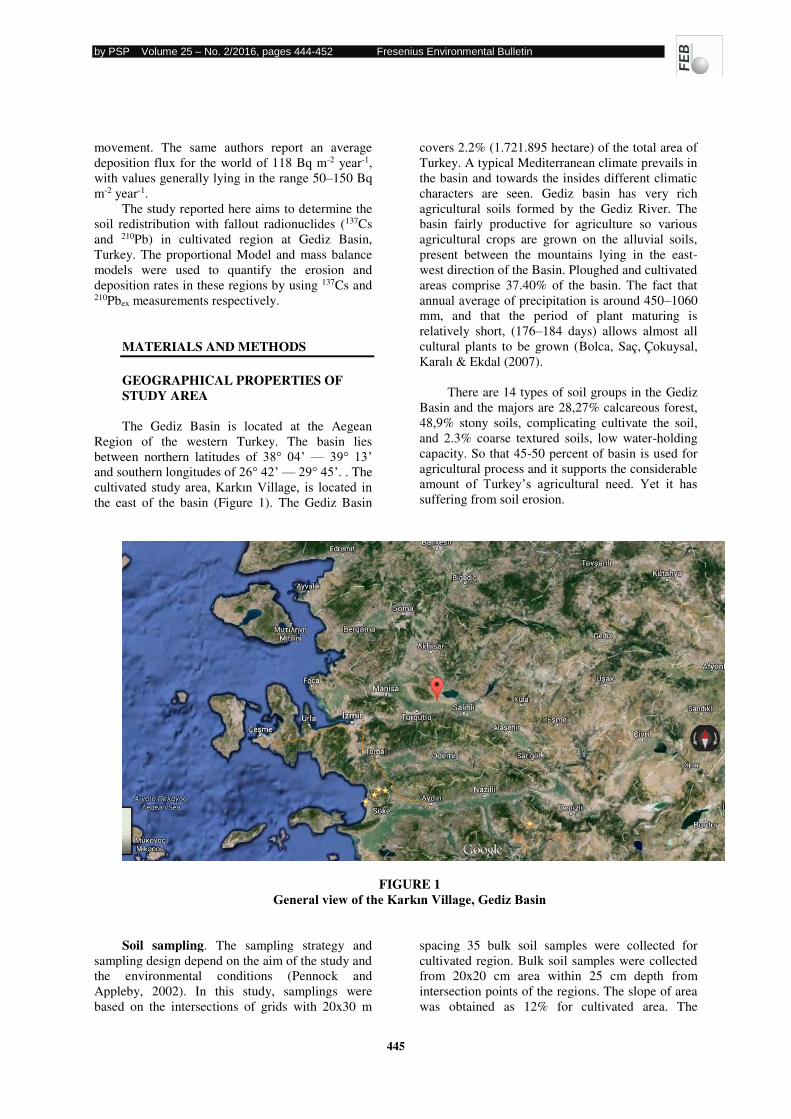
by PSP Volume 25 – No. 2/2016, pages 444-452 Fresenius Environmental Bulletin
445
movement. The same authors report an average
deposition flux for the world of 118 Bq m-2 year-1,
with values generally lying in the range 50–150 Bq
m-2 year-1.
The study reported here aims to determine the
soil redistribution with fallout radionuclides (137Cs
and 210Pb) in cultivated region at Gediz Basin,
Turkey. The proportional Model and mass balance
models were used to quantify the erosion and
deposition rates in these regions by using 137Cs and 210Pbex measurements respectively.
MATERIALS AND METHODS
GEOGRAPHICAL PROPERTIES OF STUDY AREA The Gediz Basin is located at the Aegean
Region of the western Turkey. The basin lies
between northern latitudes of 38° 04’ — 39° 13’ and southern longitudes of 26° 42’ — 29° 45’. . The
cultivated study area, Karkın Village, is located in the east of the basin (Figure 1). The Gediz Basin
covers 2.2% (1.721.895 hectare) of the total area of
Turkey. A typical Mediterranean climate prevails in
the basin and towards the insides different climatic
characters are seen. Gediz basin has very rich
agricultural soils formed by the Gediz River. The
basin fairly productive for agriculture so various
agricultural crops are grown on the alluvial soils,
present between the mountains lying in the east-
west direction of the Basin. Ploughed and cultivated
areas comprise 37.40% of the basin. The fact that
annual average of precipitation is around 450–1060
mm, and that the period of plant maturing is
relatively short, (176–184 days) allows almost all
cultural plants to be grown (Bolca, Saç, Çokuysal,
Karalı & Ekdal (2007).
There are 14 types of soil groups in the Gediz
Basin and the majors are 28,27% calcareous forest,
48,9% stony soils, complicating cultivate the soil,
and 2.3% coarse textured soils, low water-holding
capacity. So that 45-50 percent of basin is used for
agricultural process and it supports the considerable
amount of Turkey’s agricultural need. Yet it has suffering from soil erosion.
FIGURE 1
General view of the Karkın Village, Gediz Basin
Soil sampling. The sampling strategy and
sampling design depend on the aim of the study and
the environmental conditions (Pennock and
Appleby, 2002). In this study, samplings were
based on the intersections of grids with 20x30 m
spacing 35 bulk soil samples were collected for
cultivated region. Bulk soil samples were collected
from 20x20 cm area within 25 cm depth from
intersection points of the regions. The slope of area
was obtained as 12% for cultivated area. The
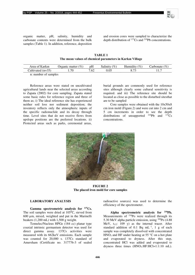
by PSP Volume 25 – No. 2/2016, pages 444-452 Fresenius Environmental Bulletin
446
organic matter, pH, salinity, humidity and
carbonate contents were determined from the bulk
samples (Table 1). In addition, reference, deposition
and erosion cores were sampled to characterize the
depth distribution of 137Cs and 210Pb concentrations.
TABLE 1 The mean values of chemical parameters in Karkın Village
Area of Karkın Organic matter (%) pH Salinity (%) Humidity (%) Carbonate (%)
Cultivated (n=35) 1.70 7.62 0.05 8.73 11.7
n: number of samples
Reference areas were stated on uncultivated
agricultural lands near the selected areas according
to Zapata (2002) for core sampling. Zapata stated
some basic rules for reference region and three of
them as; i) The ideal reference site has experienced
neither soil loss nor sediment deposition; the
inventory reflects only the atmospheric inputs of
the specific radionuclide and its decay through
time. Level sites that do not receive flows from
upslope positions are the preferred locations. ii)
Protected areas such as parks, ceremonial areas,
burial grounds are commonly used for reference
sites although clearly some cultural sensitivity is
required. and iii) The reference site should be
located as close as possible to the disturbed sitesthat
are to be sampled
Core samples were obtained with the 10x50x8
cm iron mold (Figure.2) and were cut into 2 cm and
5 cm increments in order to see the depth
distributions of unsupported 210Pb and 137Cs
concentrations.
FIGURE 2 The placed iron mold for core samples
LABORATORY ANALYSIS
Gamma spectrometric analysis for 137Cs. The soil samples were dried at 1050C, sieved from
600 µm, mixed, weighted and put in the Marinelli
beakers (1,200 mL) with 1,500 g weight. Tennelec/Nucleus HPGe (184 cc) planar type
coaxial intrinsic germanium detector was used for
direct gamma assay. 137Cs activities were
measured with its 662keV emissions. Each sample
was counted for 20,000 s. 137Cs standard of
Amersham (Certificate no. 317776-3 of sealed
radioactive sources) was used to determine the
efficiency of the spectrometer.
Alpha spectrometric analysis for 210Pb. Measurements of 210Po were realized through its
5.30 MeV alpha particle emission, using 209Po (4.88
MeV, t1/2: 109 y) as the internal tracer. After
standard addition of 0.1 Bq mL−1, 1 g of each
sample was completely dissolved with concentrated
HNO3 and HF under heating at 55 °C on a hot plate
and evaporated to dryness. After this step,
concentrated HCl was added and evaporated to
dryness three times (HNO3:HF:HCl=1:1:10 mL).
by PSP Volume 25 – No. 2/2016, pages 444-452 Fresenius Environmental Bulletin
447
Polonium was spontaneously plated on copper disks
in 0.5 M HCl in the presence of ascorbic acid to
reduce Fe+3 to Fe+2 (Flynn, 1968). The recovery
rates of standardized tracer for the soil samples
varied from 70% to 90%. Alpha activities were
measured using Ortec Octete Plus with 450 mm2
ULTRA-AS Detectors. Concentrations of 210Po in
all the samples were well above the detection limit
(0.0003 Bq). Sample count times were 86,400 s,
with counting errors in the order of ±10% or less. After the first deposition of 210Po, the residual
0.5 M HCl was kept for one year to allow 210Po in-
growth from the 210Pb contained in the solution to
search supported 210Pb in the samples. The samples
were re-plated and the 210Po activities were
determined. Well known Bateman equations were
used to obtain 210Pb activity from measured 210Po
activity (Bateman, 1910; Cetnar, 2006). The second
deposition provided information on the 210Pb
content of the samples and hence on the extent to
which the initial 210Po was supported by its
grandparent.
MATHEMATICAL MODELS USED IN THE STUDY
The proportional model for 137Cs. The
reference inventories at the sampling area should be
higher than the erosion region and higher than the
deposition sites to apply the 137Cs model. So it is
observed that some sampling points’ 137Cs
inventories are lower than reference inventory
showing the soil loss while some points getting
higher for deposition areas. The proportional model
was used widely for 137Cs to calculate the soil loss
and deposition rate all over the world. It is based on
the assumption that 137Cs fallout inputs are
completely mixed within the plough or cultivation
layer and that soil loss is directly proportional to the
reduction in the 137Cs content in the soil profile
(Saç, Uğur, Yener & Özden, (2008). The mean
annual soil loss rate Y (t ha–1 y–1) can be written as
follows: (Walling and He 199a)
(1)
where
X = the percentage reduction in total 137Cs
inventory (defined as (Aref – A)/Aref · 100)
d = the depth of the plough or cultivation
layer (m)
B = the bulk density of the soil (kg m-3)
t = the time elapsed since initiation of 137Cs
accumulation (since 1963) (year)
Aref = the local reference inventory (Bq m-2)
A = the total inventory measured at the
sampling point (Bq m-2).
The mass balance model for 210Pb. The mass
balance conversion model (Walling and He, 1999b)
was used to estimate the soil redistribution rates
(kg/m/year) from the unsupported 210Pb inventories
associated with collected soil samples. Following Walling and He the change in the
activity of accumulated 137Cs or 210Pbex A(t) (Bq m-
2) per unit area with time t (yr) at an eroding site
can be represented as:
dtetIetAtA
t
t
ttDPRdtDPR
t
t
0
,0
,
))(/(,)/(
0 )()1()()( (2)
where
R= mean annual erosion rate (kg m-2 yr-1)
D = mass depth representing the average
plough depth (kg m-2)
l= decay constant for 137Cs or 210Pbex (yr-1)
I(t) =annual 137Cs or 210Pbex deposition flux
(Bq m-2 yr-1)
= proportion of the freshly deposited 137Cs
or 210Pbex fallout removed by erosion before being
mixed into the plough layer
P = particle size correction factor
t0 (yr) = year when cultivation started
A(t0) (Bq m-2) = 210Pbex or 137Cs inventory at
t0.
can be expressed as
)1( / HReP (3)
γ is the proportion of the annual 137Cs or 210Pbex fallout susceptible to removal by erosion
prior to incorporation into the soil profile by tillage
and is dependent on the timing of cultivation and
the local rainfall regime; H (kg/m2) is the relaxation
mass depth of the initial distribution of the fallout
radionuclide in the soil profile, which can be
determined experimentally for local conditions (He
and Walling, 1997).
According to mass balance conversion model
the following parameters were obtained from the
studying area. An average plough depth (D) of 220
(kg m-2) (corresponding to an average bulk density
and a plough depth ), a value of the relaxation mass
depth (H) equal to 98.04 (kg m-2) (it was derived
from the graph of the lnA of 210Pb of reference core
vs relaxation mass depth) , a value of γ equal to 0.14 based on the relationship between the timing
of cultivation and the rainfall regime of the
sampling area and also 210Pb decay constant 0,0311
(y-1) was used. A particle size correction factor P of
1.4 was calculated by considering the enrichment of
the eroded soil in fines relative to the source
material. And also annual fallout 210Pb deposition
was determined as 116 (Bq m-1 year-1).
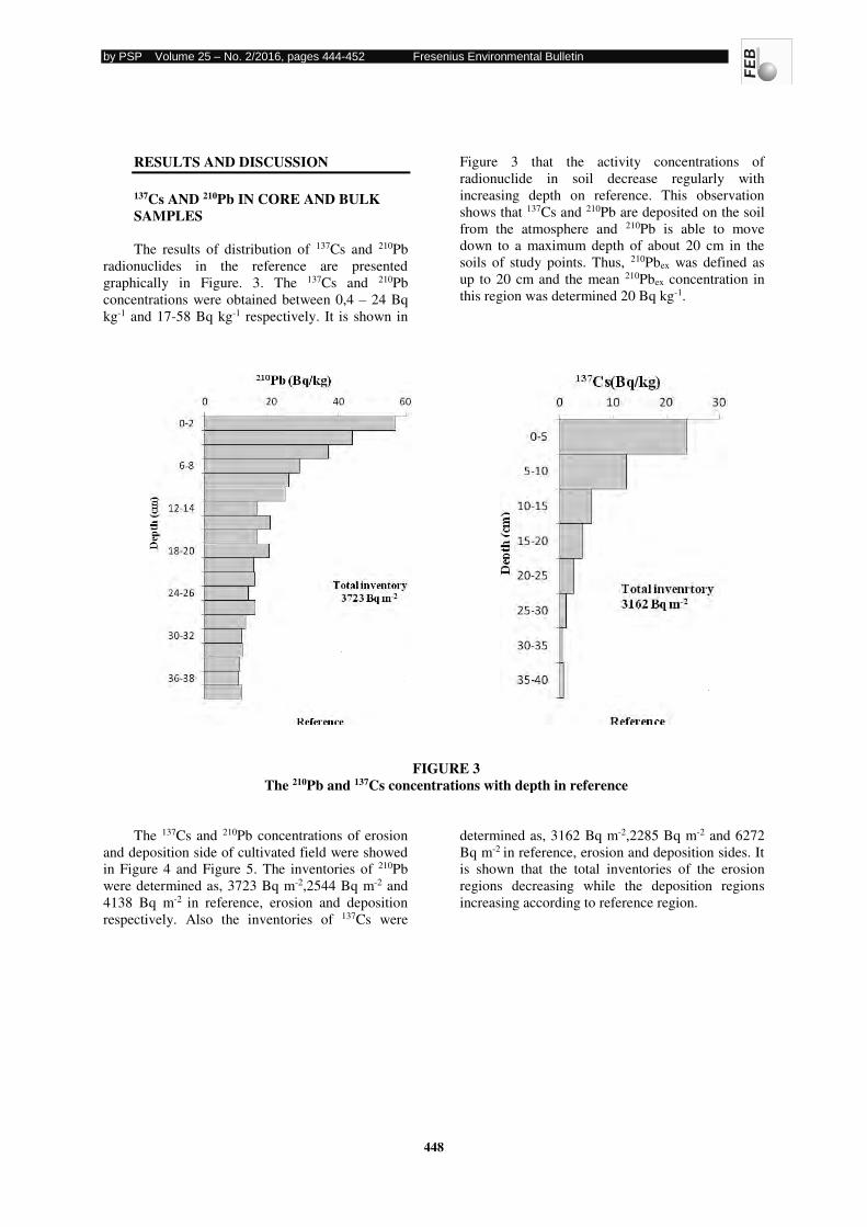
by PSP Volume 25 – No. 2/2016, pages 444-452 Fresenius Environmental Bulletin
448
RESULTS AND DISCUSSION
137Cs AND 210Pb IN CORE AND BULK SAMPLES
The results of distribution of 137Cs and 210Pb
radionuclides in the reference are presented
graphically in Figure. 3. The 137Cs and 210Pb
concentrations were obtained between 0,4 – 24 Bq
kg-1 and 17-58 Bq kg-1 respectively. It is shown in
Figure 3 that the activity concentrations of
radionuclide in soil decrease regularly with
increasing depth on reference. This observation
shows that 137Cs and 210Pb are deposited on the soil
from the atmosphere and 210Pb is able to move
down to a maximum depth of about 20 cm in the
soils of study points. Thus, 210Pbex was defined as
up to 20 cm and the mean 210Pbex concentration in
this region was determined 20 Bq kg-1.
FIGURE 3 The 210Pb and 137Cs concentrations with depth in reference
The 137Cs and 210Pb concentrations of erosion
and deposition side of cultivated field were showed
in Figure 4 and Figure 5. The inventories of 210Pb
were determined as, 3723 Bq m-2,2544 Bq m-2 and
4138 Bq m-2 in reference, erosion and deposition
respectively. Also the inventories of 137Cs were
determined as, 3162 Bq m-2,2285 Bq m-2 and 6272
Bq m-2 in reference, erosion and deposition sides. It
is shown that the total inventories of the erosion
regions decreasing while the deposition regions
increasing according to reference region.
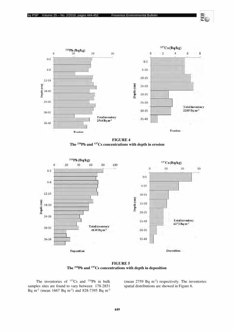
by PSP Volume 25 – No. 2/2016, pages 444-452 Fresenius Environmental Bulletin
449
FIGURE 4 The 210Pb and 137Cs concentrations with depth in erosion
FIGURE 5 The 210Pb and 137Cs concentrations with depth in deposition
The inventories of 137Cs and 210Pb in bulk
samples sites are found to vary between 178-2851
Bq m-2 (mean 1667 Bq m-2) and 828-7395 Bq m-2
(mean 2759 Bq m-2) respectively. The inventories
spatial distributions are showed in Figure 6.
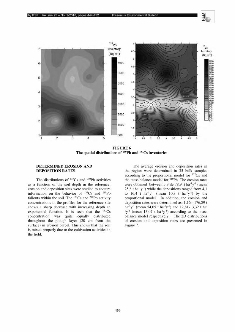
by PSP Volume 25 – No. 2/2016, pages 444-452 Fresenius Environmental Bulletin
450
FIGURE 6 The spatial distributions of 210Pb and 137Cs inventories
DETERMINED EROSION AND DEPOSITION RATES The distributions of 137Cs and 210Pb activities
as a function of the soil depth in the reference,
erosion and deposition sites were studied to acquire
information on the behavior of 137Cs and 210Pb
fallouts within the soil. The 137Cs and 210Pb activity
concentrations in the profiles for the reference site
shows a sharp decrease with increasing depth an
exponential function. It is seen that the 137Cs
concentration was quite equally distributed
throughout the plough layer (20 cm from the
surface) in erosion parcel. This shows that the soil
is mixed properly due to the cultivation activities in
the field.
The average erosion and deposition rates in
the region were determined in 35 bulk samples
according to the proportional model for 137Cs and
the mass balance model for 210Pb. The erosion rates
were obtained between 5,9 ile 78,9 t ha-1y-1 (mean
25,8 t ha-1y-1) while the depositions ranged from 4,1
to 16,4 t ha-1y-1 (mean 10,8 t ha-1y-1) by the
proportional model. In addition, the erosion and
deposition rates were determined as, 1,16 - 176,89 t
ha-1y-1 (mean 54,05 t ha-1y-1) and 12,81-13,32 t ha-
1y-1 (mean 13,07 t ha-1y-1) according to the mass
balance model respectively. The 2D distributions
of erosion and deposition rates are presented in
Figure 7.
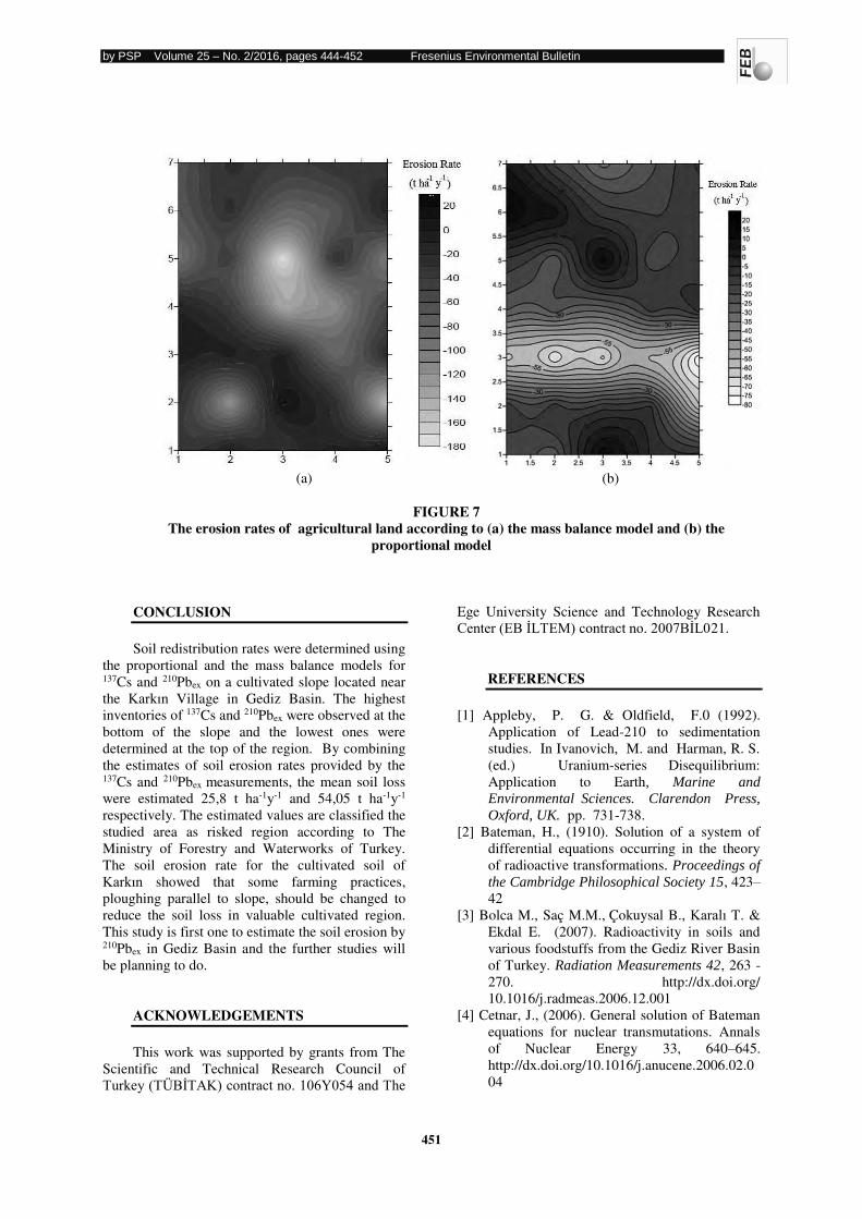
by PSP Volume 25 – No. 2/2016, pages 444-452 Fresenius Environmental Bulletin
451
(a) (b)
FIGURE 7 The erosion rates of agricultural land according to (a) the mass balance model and (b) the
proportional model
CONCLUSION
Soil redistribution rates were determined using
the proportional and the mass balance models for 137Cs and 210Pbex on a cultivated slope located near
the Karkın Village in Gediz Basin. The highest
inventories of 137Cs and 210Pbex were observed at the
bottom of the slope and the lowest ones were
determined at the top of the region. By combining
the estimates of soil erosion rates provided by the 137Cs and 210Pbex measurements, the mean soil loss
were estimated 25,8 t ha-1y-1 and 54,05 t ha-1y-1
respectively. The estimated values are classified the
studied area as risked region according to The
Ministry of Forestry and Waterworks of Turkey.
The soil erosion rate for the cultivated soil of
Karkın showed that some farming practices,
ploughing parallel to slope, should be changed to
reduce the soil loss in valuable cultivated region.
This study is first one to estimate the soil erosion by 210Pbex in Gediz Basin and the further studies will
be planning to do.
ACKNOWLEDGEMENTS
This work was supported by grants from The
Scientific and Technical Research Council of
Turkey (TÜBİTAK) contract no. 106Y054 and The
Ege University Science and Technology Research
Center (EB İLTEM) contract no. 2007BİL021.
REFERENCES
[1] Appleby, P. G. & Oldfield, F.0 (1992).
Application of Lead-210 to sedimentation
studies. In Ivanovich, M. and Harman, R. S.
(ed.) Uranium-series Disequilibrium:
Application to Earth, Marine and
Environmental Sciences. Clarendon Press,
Oxford, UK. pp. 731-738.
[2] Bateman, H., (1910). Solution of a system of
differential equations occurring in the theory
of radioactive transformations. Proceedings of
the Cambridge Philosophical Society 15, 423–42
[3] Bolca M., Saç M.M., Çokuysal B., Karalı T. &
Ekdal E. (2007). Radioactivity in soils and
various foodstuffs from the Gediz River Basin
of Turkey. Radiation Measurements 42, 263 -
270. http://dx.doi.org/
10.1016/j.radmeas.2006.12.001
[4] Cetnar, J., (2006). General solution of Bateman
equations for nuclear transmutations. Annals
of Nuclear Energy 33, 640–645.
http://dx.doi.org/10.1016/j.anucene.2006.02.0
04
by PSP Volume 25 – No. 2/2016, pages 444-452 Fresenius Environmental Bulletin
452
[5] Flynn, W.W. (1968). The determination of low
levels of polonium-210 in environmental
materials. Analytica Chimica Acta 43, 221 -
227.
[6] He, Q., & Walling, D. E. (1997). The
distribution of fallout 137Cs and 210Pb in
undisturbed and cultivated soils. Applied
Radiation and Isotopes, 48, 677–690.
http://dx.doi.org/10.1016/S0969-
8043(96)00302-8
[7] Mabit L., Benmansour M. & Walling D.E.,
(2008). Comparative advantages and
limitations of the fallout radionuclides 137Cs, 210Pbex and 7Be for assessing soil erosion and
sedimentation. Journal of Environmental
Radioactivity 99, 1799–1807.
http://dx.doi.org/10.1016/j.jenvrad.2008.08.00
9
[8] Oldeman, L.R. (1994). The global extent of soil
degradation. In: Greenland, D.J., Szabolcs, I.
(ed.), Soil Resilience and Sustainable Land
Use. CAB International, Wallingford, Oxon,
UK, pp. 99–118.
[9] Pennock, D.J. & Appleby, P.G. (2002). Site
selection and sampling design. In: Zapata, F.
(Ed.), Handbook for the Assessment of Soil
Erosion and Sedimentation Using
Environmental Radionuclides. Kluwer
Academic Publishers, pp. 15 40.
[10] Porto P., Walling D.E., Capra A., (2014).
Using 137Cs and 210Pbex measurements and
conventional surveys to investigate the
relative contributions of interrill/rill and gully
erosion to soil loss from a small cultivated
catchment in Sicily. Soil & Tillage Research
135. 18–27.
http://dx.doi.org/10.1016/j.still.2013.08.013
[11] Robbins, R.A. (1978). Geochemical and
geophysical application of radioactive lead. In:
Nriagu, J.O. (ed.), The Biogeochemistry of
Lead in the Environment. Elsevier,
Amsterdam, pp. 286–383.
[12] Saç M. M., Uğur A., Yener G., Özden B. (2008). Estimates of soil erosion using
cesium-137 tracer models. Environ Monit
Assess 136, 461 - 467.
http://dx.doi.org/10.1007/s10661-007-9700-8
[13] Walling D.E., He Q., (1999a). Improved
models for estimating soil erosion rates from
Cesium-137 measurements. J Environ Qual
28,611–622
http://dx.doi.org/10.2134/jeq1999.0047242500
2800020027x
[14] Walling, D.E., He Q., (1999b). Using fallout
lead-210 measurements to estimate soil
erosion on cultivated land. Soil Science
Society of America Journal 63, 1404 - 1412.
http://dx.doi.org/10.2136/sssaj1999.6351404x
[15] Zapata F., (2002) Handbook for the
Assessment of Soil Erosion and Sedimentation
Using Environmental Radionuclides, Kluwer
Academic Publishers, Boston.
Received: 22.06.2015 Accepted: 06.01.2016 CORRESPONDING AUTHOR
Manav Ramazan Ege University
Institute of Nuclear Sciences
35100 Bornova, İzmir – TURKEY
e-mail address: [email protected]
by PSP Volume 25 – No. 2/2016, pages 453-463 Fresenius Environmental Bulletin
453
DISTRIBUTION AND BIOAVAILABILITY OF NITROGEN AND
PHOSPHORUS FRACTIONS IN STREET DUSTS OF
MEGA-CITY, CHENGDU, SOUTHWEST CHINA
Bin Zhanga, Chi Xuc, Shumin Wangb,*, Chunmei Weia
a School of food biotechnology of Xihua University, Chengdu 610039, China
b Chongqing Key Laboratory of Environmental Material and Restoration Technology, Chongqing University of Arts and Sciences,
Chongqing 402160, China c Xihua University of Architecture and Civil Engineering, Sichuan Chengdu, 610039, China
ABSTRACT
Forty-two street dust samples of Chengdu City were
collected from impervious areas with seven different
urban land-use types. The studies on spatial
distribution, correlation and bioavailability of
nitrogen and phosphorus species were made
according to the analyzed data. The results showed
that total nitrogen (TN) was composed mainly of
organic matter-sulfide form (OSF-N) and weak acid
extractable form (WAEF-N) while total phosphorus
(TP) and inorganic phosphorus (IP) consisted chiefly
of phosphorus bound to calcium was extracted by HCl
(Ca-P), and the spatial variability of nitrogen and
phosphorus species contents was greatly affected by
the mode of urban land-use type. In addition, there are
significant correlations among partial nitrogen and
phosphorus forms in street dusts. Corresponding to
different urban land-use types, the average ratios of
bioavailable nitrogen content (the sum of
ion-extractable form (IEF-N), WAEF-N,
iron-manganese oxides form (IMOF-N), and OSF-N)
to TN were 40.10%, 40.34%, 41.14%, 38.89%,
47.47%, 34.61%, and 31.00%, respectively, while the
mean ratios of bioavailable phosphorus content ( the
sum of Fe/Al-P and OP) to TP, were equal to 32.95%,
17.67%, 32.87%, 36.83%, 32.20%, 45.52%, and
30.58%, respectively. Higher bioavailable nitrogen
and phosphorus contents can also cause the
eutrophication of receiving water bodies.
KEYWORDS: Street dust; Nitrogen and phosphorus fractions;
Bioavailability; Chengdu City.
INTRODUCTION
The rapid increase of impervious land in the city
changes surface accumulation and the flush law of
pollutants, and leads to the “source”, “process” and “sink” of the nonpoint source pollution changed [1]. As an important carrier of pollutants, street dust is one
of the typical nonpoint source pollution, and it is
closely related to water and air pollution. On the one
hand, Street dust is transported into the receiving
waters during rainfall and affects the stream water
quality and aquatic biota markedly. Urban runoff has
been deemed as one of the leading sources of water
quality impairment for rivers, lakes and estuaries. On
the other hand, under the influence of wind, traffic
flow and anthropic activity, the street dust may be
re-suspended and affects the atmospheric
environmental quality and weather. Therefore, the
quality of street dust is related to urban aquatic,
atmospheric and ecological environment including
human health [2].
Nitrogen and phosphorus are major nutrients for
terrestrial and aquatic plants and animals, and their
excess supply poses environmental risks because it
may cause eutrophication of surface water bodies.
Nowadays, most cities at home and abroad are more
or less troubled by eutrophication. In the process of
controlling exogenous input load, it is a very
meaningful work on scientific understanding and
evaluation the contribution of nitrogen and
phosphorus from street dust and their biological
effectiveness. Many studies on street dust have
focused on trace metal elements concentration,
distribution and source identification in the last
decades [3-17]. However, there is little information
on nitrogen and phosphorus in the street dust [2,
18-21]. During rain/storm/street-washing events, the
street dust particles laden with nitrogen and
phosphorus are washed off and finally end up in
receiving water bodies and may cause eutrophication
of the receiving water bodies. Not all of the nitrogen
and phosphorus fractions can be released into the
water, the nitrogen and phosphorus behavior in street
dust for promoting urban water bodies eutrophication
can be more efficiently evaluated based on the their
fractions, instead of the total nitrogen or total
phosphorus content.
Chengdu, one of the most crowded cities in the
world, has experienced a rapid urbanization and
industrialization in the last decades. The rapid growth
by PSP Volume 25 – No. 2/2016, pages 453-463 Fresenius Environmental Bulletin
454
of industry, population and vehicle exerts a heavy
pressure on its urban environment. The aims of this
study were to investigate the characteristics of the
nitrogen and phosphorus fractions in the street dust
samples collected from Chengdu city, to analyze their
biological effectiveness. This study will provide a
scientific basis for estimating nonpoint source
pollution load, pollution assessment and control
measures.
MATERIALS AND METHODS
Study area. Chengdu (30°05′-31°26′N,
102°54′ -104°53′E), the capital of Sichuan
province, is located in the southwest of China.
Geomorphologically, it is high to the northwest and
low to the southeast, not far from the western slopes
of the Longmen Mountains. With a typical continental
monsoon climate of northern temperate zone, there
are four distinct seasons in Chengdu. The average
temperature ranges from 5 °C in winter to 26 °C in
summer. The average annual precipitation is 918 mm.
Rainfall mainly concentrated from July to August.
The least rainfall concentrated from December to
March. In the present study, street dust samples were
collected from various areas with different land uses
(educational district, commercial district, scenic parks,
traffic pivotal district, industrial district, residential
district, and peri-urban district).
Sampling and analytical procedures. Although
there was no strict functional classification in urban
areas in Chengdu, forty-two samples were collected at
different districts with different land use: Xihua
university and Southwest Jiaotong University
(educational district, abbreviation as ED, S1-S6),
Chunxi road and Babaoroad commercial center
district (commercial district, abbreviation as CD,
S7-S12), Du Fu Thatched Cottage and Temple of
Marquis scenic districts (scenic parks, abbreviation as
SP, S13-S18), Chengdu north railway station and
Xinnanmen bus station (traffic pivotal district,
abbreviation as TD, S19-S24), Pixian county modern
industrial port of destination and Shuangliu airport
industrial park (industrial district, abbreviation as ID,
S25-S30), Shahepu residential district and A loop
section of East residential district (residential district,
abbreviation as RD, S31-S36), and Sandaoyan town
and Youai town (peri-urban district, abbreviation as
PD, S37-S42) in August 2012 in Chengdu, China.
Forty-two samples were collected on pavements next
to roads at periods when no rain had occurred during
the previous week in Chengdu. At every sampling site,
more than 300 g of street dust composite sample was
collected by sweeping using polyethylene brush and
tray from five to eight points of road/pavement edges
within the scope of 10m×10m. All the samples were
stored in the sealed polyethylene bags, labeled and
then transported to the laboratory. The samples were
air-dried in the laboratory for 2weeks. Dried samples
were grinded by a porcelain mill and then passed
through a 100-mesh sieve before analyzing. Detailed
locations of sampling sites are shown in Fig.1. The
pH of all the samples was taken in the ratio (w: v),
sample (1): distilled water (2.5) [22]. The organic
matters (OM) were measured by Kjeldahl and
potassium dichromate-external heating method,
separately [23].
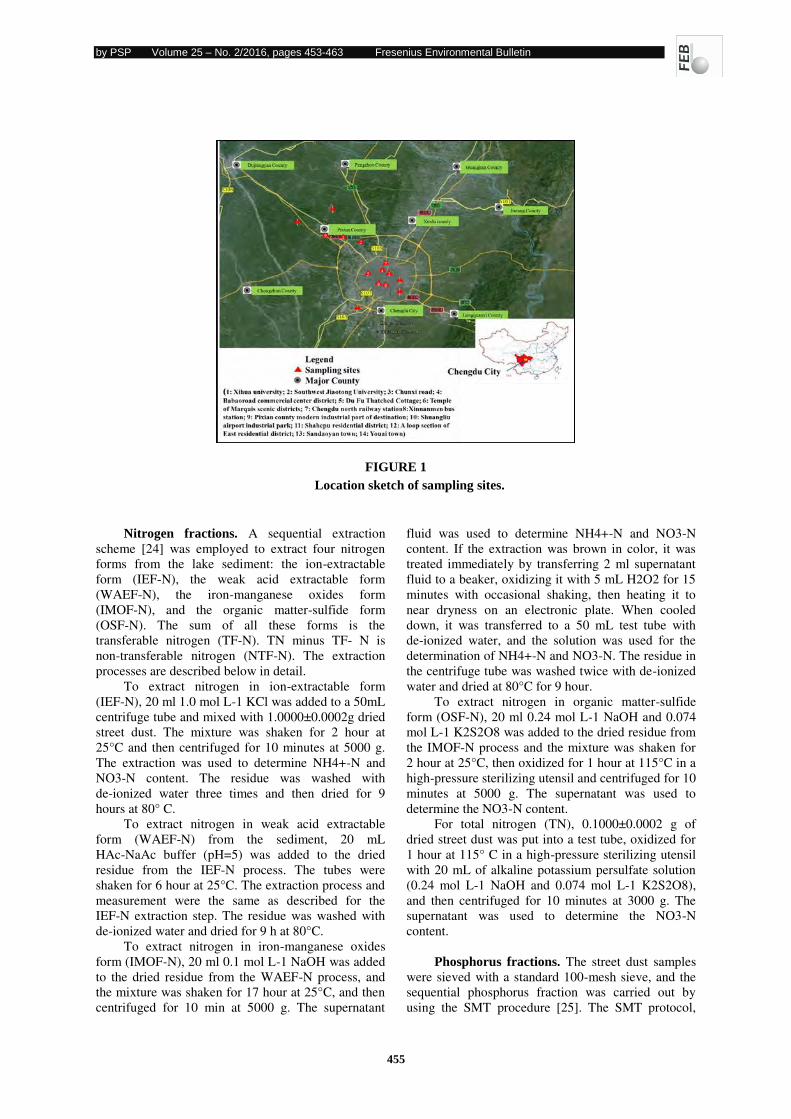
by PSP Volume 25 – No. 2/2016, pages 453-463 Fresenius Environmental Bulletin
455
FIGURE 1
Location sketch of sampling sites.
Nitrogen fractions. A sequential extraction
scheme [24] was employed to extract four nitrogen
forms from the lake sediment: the ion-extractable
form (IEF-N), the weak acid extractable form
(WAEF-N), the iron-manganese oxides form
(IMOF-N), and the organic matter-sulfide form
(OSF-N). The sum of all these forms is the
transferable nitrogen (TF-N). TN minus TF- N is
non-transferable nitrogen (NTF-N). The extraction
processes are described below in detail.
To extract nitrogen in ion-extractable form
(IEF-N), 20 ml 1.0 mol L-1 KCl was added to a 50mL
centrifuge tube and mixed with 1.0000±0.0002g dried
street dust. The mixture was shaken for 2 hour at
25°C and then centrifuged for 10 minutes at 5000 g.
The extraction was used to determine NH4+-N and
NO3-N content. The residue was washed with
de-ionized water three times and then dried for 9
hours at 80° C.
To extract nitrogen in weak acid extractable
form (WAEF-N) from the sediment, 20 mL
HAc-NaAc buffer (pH=5) was added to the dried
residue from the IEF-N process. The tubes were
shaken for 6 hour at 25°C. The extraction process and
measurement were the same as described for the
IEF-N extraction step. The residue was washed with
de-ionized water and dried for 9 h at 80°C.
To extract nitrogen in iron-manganese oxides
form (IMOF-N), 20 ml 0.1 mol L-1 NaOH was added
to the dried residue from the WAEF-N process, and
the mixture was shaken for 17 hour at 25°C, and then
centrifuged for 10 min at 5000 g. The supernatant
fluid was used to determine NH4+-N and NO3-N
content. If the extraction was brown in color, it was
treated immediately by transferring 2 ml supernatant
fluid to a beaker, oxidizing it with 5 mL H2O2 for 15
minutes with occasional shaking, then heating it to
near dryness on an electronic plate. When cooled
down, it was transferred to a 50 mL test tube with
de-ionized water, and the solution was used for the
determination of NH4+-N and NO3-N. The residue in
the centrifuge tube was washed twice with de-ionized
water and dried at 80°C for 9 hour.
To extract nitrogen in organic matter-sulfide
form (OSF-N), 20 ml 0.24 mol L-1 NaOH and 0.074
mol L-1 K2S2O8 was added to the dried residue from
the IMOF-N process and the mixture was shaken for
2 hour at 25°C, then oxidized for 1 hour at 115°C in a
high-pressure sterilizing utensil and centrifuged for 10
minutes at 5000 g. The supernatant was used to
determine the NO3-N content.
For total nitrogen (TN), 0.1000±0.0002 g of
dried street dust was put into a test tube, oxidized for
1 hour at 115° C in a high-pressure sterilizing utensil
with 20 mL of alkaline potassium persulfate solution
(0.24 mol L-1 NaOH and 0.074 mol L-1 K2S2O8),
and then centrifuged for 10 minutes at 3000 g. The
supernatant was used to determine the NO3-N
content.
Phosphorus fractions. The street dust samples
were sieved with a standard 100-mesh sieve, and the
sequential phosphorus fraction was carried out by
using the SMT procedure [25]. The SMT protocol,
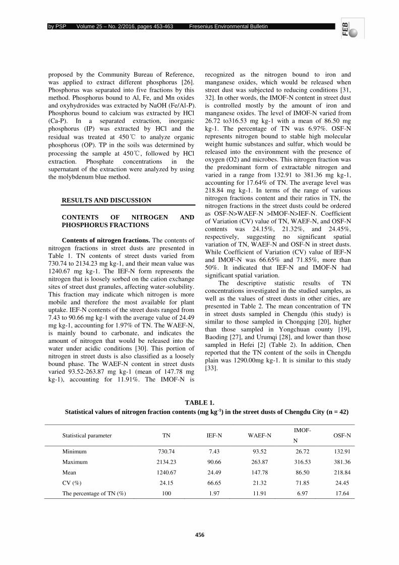
by PSP Volume 25 – No. 2/2016, pages 453-463 Fresenius Environmental Bulletin
456
proposed by the Community Bureau of Reference,
was applied to extract different phosphorus [26].
Phosphorus was separated into five fractions by this
method. Phosphorus bound to Al, Fe, and Mn oxides
and oxyhydroxides was extracted by NaOH (Fe/Al-P).
Phosphorus bound to calcium was extracted by HCl
(Ca-P). In a separated extraction, inorganic
phosphorus (IP) was extracted by HCl and the
residual was treated at 450℃ to analyze organic
phosphorus (OP). TP in the soils was determined by
processing the sample at 450℃, followed by HCl
extraction. Phosphate concentrations in the
supernatant of the extraction were analyzed by using
the molybdenum blue method.
RESULTS AND DISCUSSION
CONTENTS OF NITROGEN AND
PHOSPHORUS FRACTIONS
Contents of nitrogen fractions. The contents of
nitrogen fractions in street dusts are presented in
Table 1. TN contents of street dusts varied from
730.74 to 2134.23 mg kg-1, and their mean value was
1240.67 mg kg-1. The IEF-N form represents the
nitrogen that is loosely sorbed on the cation exchange
sites of street dust granules, affecting water-solubility.
This fraction may indicate which nitrogen is more
mobile and therefore the most available for plant
uptake. IEF-N contents of the street dusts ranged from
7.43 to 90.66 mg kg-1 with the average value of 24.49
mg kg-1, accounting for 1.97% of TN. The WAEF-N,
is mainly bound to carbonate, and indicates the
amount of nitrogen that would be released into the
water under acidic conditions [30]. This portion of
nitrogen in street dusts is also classified as a loosely
bound phase. The WAEF-N content in street dusts
varied 93.52-263.87 mg kg-1 (mean of 147.78 mg
kg-1), accounting for 11.91%. The IMOF-N is
recognized as the nitrogen bound to iron and
manganese oxides, which would be released when
street dust was subjected to reducing conditions [31,
32]. In other words, the IMOF-N content in street dust
is controlled mostly by the amount of iron and
manganese oxides. The level of IMOF-N varied from
26.72 to316.53 mg kg-1 with a mean of 86.50 mg
kg-1. The percentage of TN was 6.97%. OSF-N
represents nitrogen bound to stable high molecular
weight humic substances and sulfur, which would be
released into the environment with the presence of
oxygen (O2) and microbes. This nitrogen fraction was
the predominant form of extractable nitrogen and
varied in a range from 132.91 to 381.36 mg kg-1,
accounting for 17.64% of TN. The average level was
218.84 mg kg-1. In terms of the range of various
nitrogen fractions content and their ratios in TN, the
nitrogen fractions in the street dusts could be ordered
as OSF-N>WAEF-N >IMOF-N>IEF-N. Coefficient
of Variation (CV) value of TN, WAEF-N, and OSF-N
contents was 24.15%, 21.32%, and 24.45%,
respectively, suggesting no significant spatial
variation of TN, WAEF-N and OSF-N in street dusts.
While Coefficient of Variation (CV) value of IEF-N
and IMOF-N was 66.65% and 71.85%, more than
50%. It indicated that IEF-N and IMOF-N had
significant spatial variation.
The descriptive statistic results of TN
concentrations investigated in the studied samples, as
well as the values of street dusts in other cities, are
presented in Table 2. The mean concentration of TN
in street dusts sampled in Chengdu (this study) is
similar to those sampled in Chongqing [20], higher
than those sampled in Yongchuan county [19],
Baoding [27], and Urumqi [28], and lower than those
sampled in Hefei [2] (Table 2). In addition, Chen
reported that the TN content of the soils in Chengdu
plain was 1290.00mg kg-1. It is similar to this study
[33].
TABLE 1.
Statistical values of nitrogen fraction contents (mg kg-1) in the street dusts of Chengdu City (n = 42)
Statistical parameter TN IEF-N WAEF-N IMOF-
N OSF-N
Minimum 730.74 7.43 93.52 26.72 132.91
Maximum 2134.23 90.66 263.87 316.53 381.36
Mean 1240.67 24.49 147.78 86.50 218.84
CV (%) 24.15 66.65 21.32 71.85 24.45
The percentage of TN (%) 100 1.97 11.91 6.97 17.64
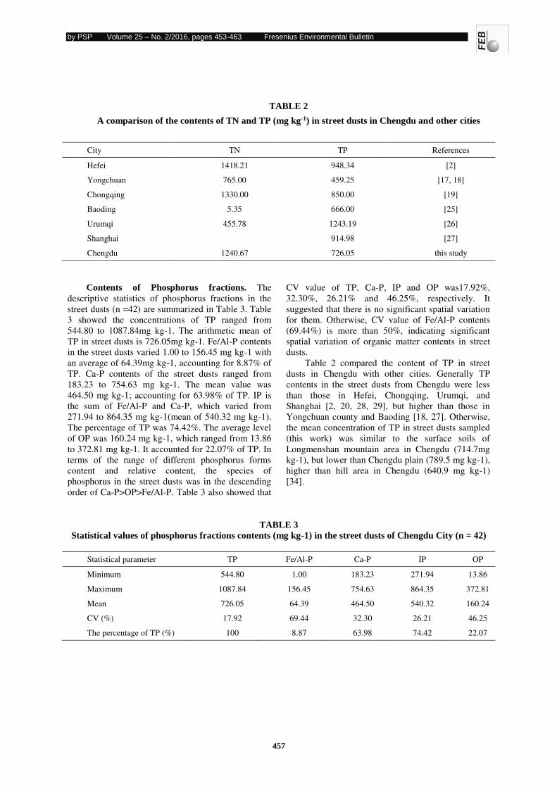
by PSP Volume 25 – No. 2/2016, pages 453-463 Fresenius Environmental Bulletin
457
TABLE 2
A comparison of the contents of TN and TP (mg kg-1) in street dusts in Chengdu and other cities
City TN TP References
Hefei 1418.21 948.34 [2]
Yongchuan 765.00 459.25 [17, 18]
Chongqing 1330.00 850.00 [19]
Baoding 5.35 666.00 [25]
Urumqi 455.78 1243.19 [26]
Shanghai 914.98 [27]
Chengdu 1240.67 726.05 this study
Contents of Phosphorus fractions. The
descriptive statistics of phosphorus fractions in the
street dusts (n =42) are summarized in Table 3. Table
3 showed the concentrations of TP ranged from
544.80 to 1087.84mg kg-1. The arithmetic mean of
TP in street dusts is 726.05mg kg-1. Fe/Al-P contents
in the street dusts varied 1.00 to 156.45 mg kg-1 with
an average of 64.39mg kg-1, accounting for 8.87% of
TP. Ca-P contents of the street dusts ranged from
183.23 to 754.63 mg kg-1. The mean value was
464.50 mg kg-1; accounting for 63.98% of TP. IP is
the sum of Fe/Al-P and Ca-P, which varied from
271.94 to 864.35 mg kg-1(mean of 540.32 mg kg-1).
The percentage of TP was 74.42%. The average level
of OP was 160.24 mg kg-1, which ranged from 13.86
to 372.81 mg kg-1. It accounted for 22.07% of TP. In
terms of the range of different phosphorus forms
content and relative content, the species of
phosphorus in the street dusts was in the descending
order of Ca-P>OP>Fe/Al-P. Table 3 also showed that
CV value of TP, Ca-P, IP and OP was17.92%,
32.30%, 26.21% and 46.25%, respectively. It
suggested that there is no significant spatial variation
for them. Otherwise, CV value of Fe/Al-P contents
(69.44%) is more than 50%, indicating significant
spatial variation of organic matter contents in street
dusts.
Table 2 compared the content of TP in street
dusts in Chengdu with other cities. Generally TP
contents in the street dusts from Chengdu were less
than those in Hefei, Chongqing, Urumqi, and
Shanghai [2, 20, 28, 29], but higher than those in
Yongchuan county and Baoding [18, 27]. Otherwise,
the mean concentration of TP in street dusts sampled
(this work) was similar to the surface soils of
Longmenshan mountain area in Chengdu (714.7mg
kg-1), but lower than Chengdu plain (789.5 mg kg-1),
higher than hill area in Chengdu (640.9 mg kg-1)
[34].
TABLE 3
Statistical values of phosphorus fractions contents (mg kg-1) in the street dusts of Chengdu City (n = 42)
Statistical parameter TP Fe/Al-P Ca-P IP OP
Minimum 544.80 1.00 183.23 271.94 13.86
Maximum 1087.84 156.45 754.63 864.35 372.81
Mean 726.05 64.39 464.50 540.32 160.24
CV (%) 17.92 69.44 32.30 26.21 46.25
The percentage of TP (%) 100 8.87 63.98 74.42 22.07
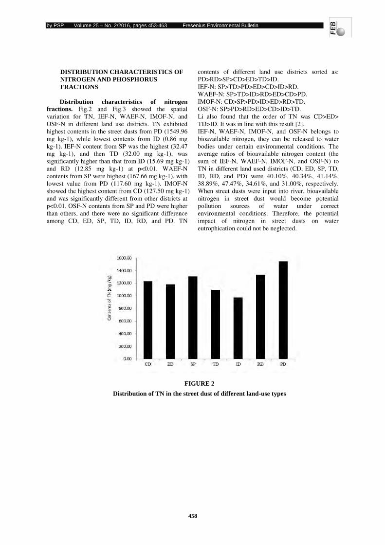
by PSP Volume 25 – No. 2/2016, pages 453-463 Fresenius Environmental Bulletin
458
DISTRIBUTION CHARACTERISTICS OF
NITROGEN AND PHOSPHORUS
FRACTIONS
Distribution characteristics of nitrogen fractions. Fig.2 and Fig.3 showed the spatial
variation for TN, IEF-N, WAEF-N, IMOF-N, and
OSF-N in different land use districts. TN exhibited
highest contents in the street dusts from PD (1549.96
mg kg-1), while lowest contents from ID (0.86 mg
kg-1). IEF-N content from SP was the highest (32.47
mg kg-1), and then TD (32.00 mg kg-1), was
significantly higher than that from ID (15.69 mg kg-1)
and RD (12.85 mg kg-1) at p<0.01. WAEF-N
contents from SP were highest (167.66 mg kg-1), with
lowest value from PD (117.60 mg kg-1). IMOF-N
showed the highest content from CD (127.50 mg kg-1)
and was significantly different from other districts at
p<0.01. OSF-N contents from SP and PD were higher
than others, and there were no significant difference
among CD, ED, SP, TD, ID, RD, and PD. TN
contents of different land use districts sorted as:
PD>RD>SP>CD>ED>TD>ID.
IEF-N: SP>TD>PD>ED>CD>ID>RD.
WAEF-N: SP>TD>ID>RD>ED>CD>PD.
IMOF-N: CD>SP>PD>ID>ED>RD>TD.
OSF-N: SP>PD>RD>ED>CD>ID>TD.
Li also found that the order of TN was CD>ED>
TD>ID. It was in line with this result [2].
IEF-N, WAEF-N, IMOF-N, and OSF-N belongs to
bioavailable nitrogen, they can be released to water
bodies under certain environmental conditions. The
average ratios of bioavailable nitrogen content (the
sum of IEF-N, WAEF-N, IMOF-N, and OSF-N) to
TN in different land used districts (CD, ED, SP, TD,
ID, RD, and PD) were 40.10%, 40.34%, 41.14%,
38.89%, 47.47%, 34.61%, and 31.00%, respectively.
When street dusts were input into river, bioavailable
nitrogen in street dust would become potential
pollution sources of water under correct
environmental conditions. Therefore, the potential
impact of nitrogen in street dusts on water
eutrophication could not be neglected.
FIGURE 2
Distribution of TN in the street dust of different land-use types
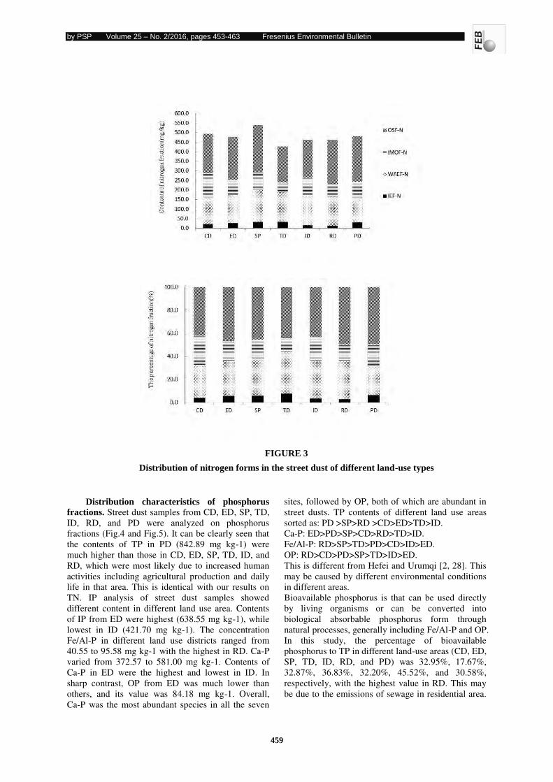
by PSP Volume 25 – No. 2/2016, pages 453-463 Fresenius Environmental Bulletin
459
FIGURE 3
Distribution of nitrogen forms in the street dust of different land-use types
Distribution characteristics of phosphorus
fractions. Street dust samples from CD, ED, SP, TD,
ID, RD, and PD were analyzed on phosphorus
fractions (Fig.4 and Fig.5). It can be clearly seen that
the contents of TP in PD (842.89 mg kg-1) were
much higher than those in CD, ED, SP, TD, ID, and
RD, which were most likely due to increased human
activities including agricultural production and daily
life in that area. This is identical with our results on
TN. IP analysis of street dust samples showed
different content in different land use area. Contents
of IP from ED were highest (638.55 mg kg-1), while
lowest in ID (421.70 mg kg-1). The concentration
Fe/Al-P in different land use districts ranged from
40.55 to 95.58 mg kg-1 with the highest in RD. Ca-P
varied from 372.57 to 581.00 mg kg-1. Contents of
Ca-P in ED were the highest and lowest in ID. In
sharp contrast, OP from ED was much lower than
others, and its value was 84.18 mg kg-1. Overall,
Ca-P was the most abundant species in all the seven
sites, followed by OP, both of which are abundant in
street dusts. TP contents of different land use areas
sorted as: PD >SP>RD >CD>ED>TD>ID.
Ca-P: ED>PD>SP>CD>RD>TD>ID.
Fe/Al-P: RD>SP>TD>PD>CD>ID>ED.
OP: RD>CD>PD>SP>TD>ID>ED.
This is different from Hefei and Urumqi [2, 28]. This
may be caused by different environmental conditions
in different areas.
Bioavailable phosphorus is that can be used directly
by living organisms or can be converted into
biological absorbable phosphorus form through
natural processes, generally including Fe/Al-P and OP.
In this study, the percentage of bioavailable
phosphorus to TP in different land-use areas (CD, ED,
SP, TD, ID, RD, and PD) was 32.95%, 17.67%,
32.87%, 36.83%, 32.20%, 45.52%, and 30.58%,
respectively, with the highest value in RD. This may
be due to the emissions of sewage in residential area.
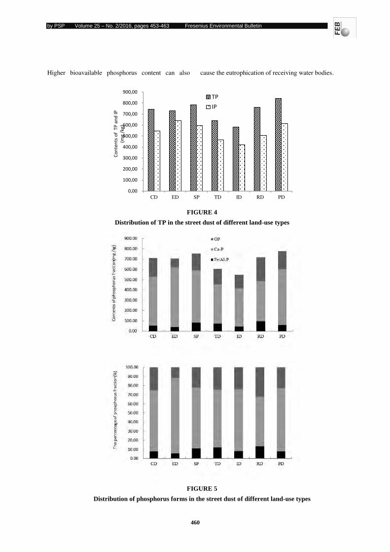
by PSP Volume 25 – No. 2/2016, pages 453-463 Fresenius Environmental Bulletin
460
Higher bioavailable phosphorus content can also cause the eutrophication of receiving water bodies.
FIGURE 4
Distribution of TP in the street dust of different land-use types
FIGURE 5
Distribution of phosphorus forms in the street dust of different land-use types
0,00
100,00
200,00
300,00
400,00
500,00
600,00
700,00
800,00
900,00
CD ED SP TD ID RD PD
TP
IP
Co
nte
nts
of
TP
an
d I
P
(mg
/kg
)
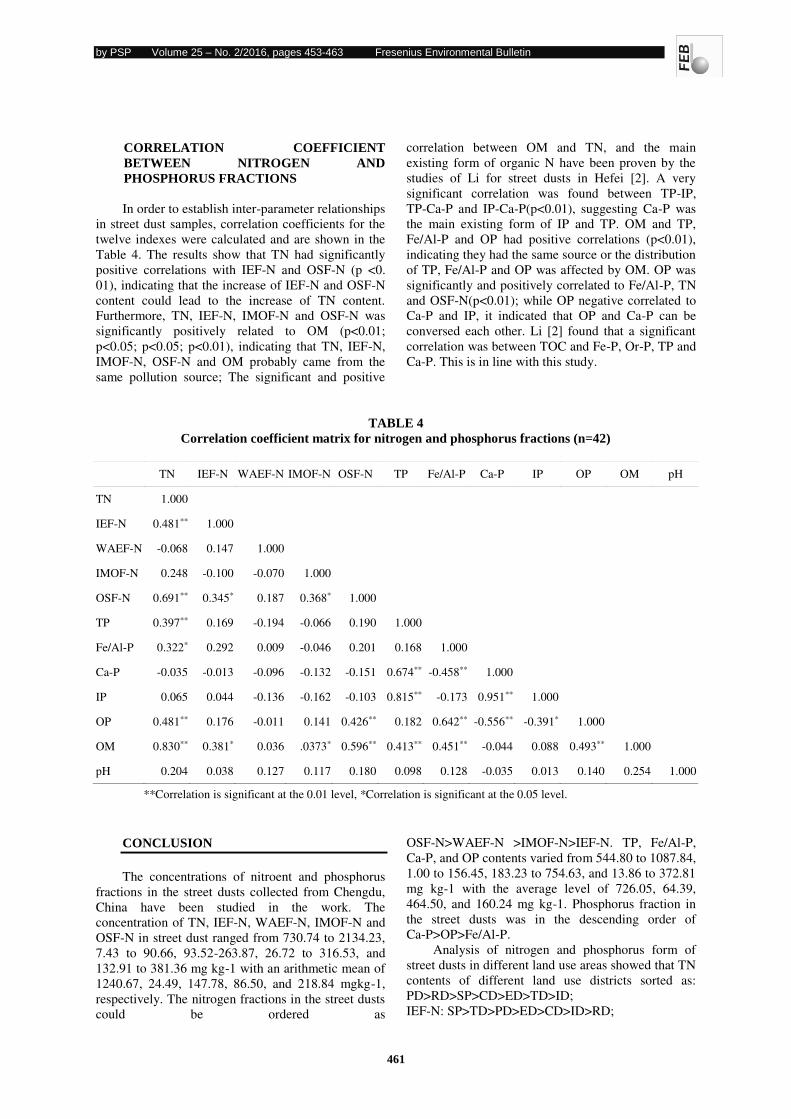
by PSP Volume 25 – No. 2/2016, pages 453-463 Fresenius Environmental Bulletin
461
CORRELATION COEFFICIENT
BETWEEN NITROGEN AND
PHOSPHORUS FRACTIONS
In order to establish inter-parameter relationships
in street dust samples, correlation coefficients for the
twelve indexes were calculated and are shown in the
Table 4. The results show that TN had significantly
positive correlations with IEF-N and OSF-N (p <0.
01), indicating that the increase of IEF-N and OSF-N
content could lead to the increase of TN content.
Furthermore, TN, IEF-N, IMOF-N and OSF-N was
significantly positively related to OM (p<0.01;
p<0.05; p<0.05; p<0.01), indicating that TN, IEF-N,
IMOF-N, OSF-N and OM probably came from the
same pollution source; The significant and positive
correlation between OM and TN, and the main
existing form of organic N have been proven by the
studies of Li for street dusts in Hefei [2]. A very
significant correlation was found between TP-IP,
TP-Ca-P and IP-Ca-P(p<0.01), suggesting Ca-P was
the main existing form of IP and TP. OM and TP,
Fe/Al-P and OP had positive correlations (p<0.01),
indicating they had the same source or the distribution
of TP, Fe/Al-P and OP was affected by OM. OP was
significantly and positively correlated to Fe/Al-P, TN
and OSF-N(p<0.01); while OP negative correlated to
Ca-P and IP, it indicated that OP and Ca-P can be
conversed each other. Li [2] found that a significant
correlation was between TOC and Fe-P, Or-P, TP and
Ca-P. This is in line with this study.
TABLE 4
Correlation coefficient matrix for nitrogen and phosphorus fractions (n=42)
TN IEF-N WAEF-N IMOF-N OSF-N TP Fe/Al-P Ca-P IP OP OM pH
TN 1.000
IEF-N 0.481** 1.000
WAEF-N -0.068 0.147 1.000
IMOF-N 0.248 -0.100 -0.070 1.000
OSF-N 0.691** 0.345* 0.187 0.368* 1.000
TP 0.397** 0.169 -0.194 -0.066 0.190 1.000
Fe/Al-P 0.322* 0.292 0.009 -0.046 0.201 0.168 1.000
Ca-P -0.035 -0.013 -0.096 -0.132 -0.151 0.674** -0.458** 1.000
IP 0.065 0.044 -0.136 -0.162 -0.103 0.815** -0.173 0.951** 1.000
OP 0.481** 0.176 -0.011 0.141 0.426** 0.182 0.642** -0.556** -0.391* 1.000
OM 0.830** 0.381* 0.036 .0373* 0.596** 0.413** 0.451** -0.044 0.088 0.493** 1.000
pH 0.204 0.038 0.127 0.117 0.180 0.098 0.128 -0.035 0.013 0.140 0.254 1.000
**Correlation is significant at the 0.01 level, *Correlation is significant at the 0.05 level.
CONCLUSION
The concentrations of nitroent and phosphorus
fractions in the street dusts collected from Chengdu,
China have been studied in the work. The
concentration of TN, IEF-N, WAEF-N, IMOF-N and
OSF-N in street dust ranged from 730.74 to 2134.23,
7.43 to 90.66, 93.52-263.87, 26.72 to 316.53, and
132.91 to 381.36 mg kg-1 with an arithmetic mean of
1240.67, 24.49, 147.78, 86.50, and 218.84 mgkg-1,
respectively. The nitrogen fractions in the street dusts
could be ordered as
OSF-N>WAEF-N >IMOF-N>IEF-N. TP, Fe/Al-P,
Ca-P, and OP contents varied from 544.80 to 1087.84,
1.00 to 156.45, 183.23 to 754.63, and 13.86 to 372.81
mg kg-1 with the average level of 726.05, 64.39,
464.50, and 160.24 mg kg-1. Phosphorus fraction in
the street dusts was in the descending order of
Ca-P>OP>Fe/Al-P.
Analysis of nitrogen and phosphorus form of
street dusts in different land use areas showed that TN
contents of different land use districts sorted as:
PD>RD>SP>CD>ED>TD>ID;
IEF-N: SP>TD>PD>ED>CD>ID>RD;
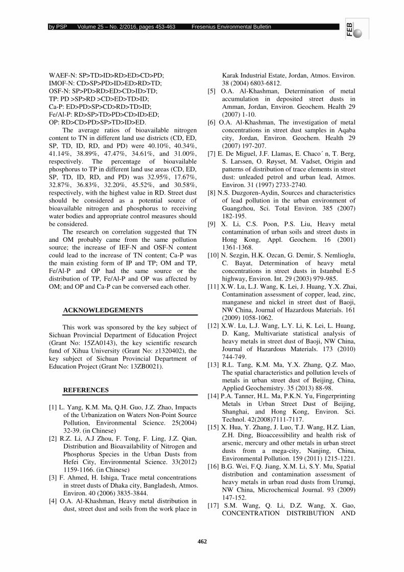
by PSP Volume 25 – No. 2/2016, pages 453-463 Fresenius Environmental Bulletin
462
WAEF-N: SP>TD>ID>RD>ED>CD>PD;
IMOF-N: CD>SP>PD>ID>ED>RD>TD;
OSF-N: SP>PD>RD>ED>CD>ID>TD;
TP: PD >SP>RD >CD>ED>TD>ID;
Ca-P: ED>PD>SP>CD>RD>TD>ID;
Fe/Al-P: RD>SP>TD>PD>CD>ID>ED;
OP: RD>CD>PD>SP>TD>ID>ED.
The average ratios of bioavailable nitrogen
content to TN in different land use districts (CD, ED,
SP, TD, ID, RD, and PD) were 40.10%, 40.34%,
41.14%, 38.89%, 47.47%, 34.61%, and 31.00%,
respectively. The percentage of bioavailable
phosphorus to TP in different land use areas (CD, ED,
SP, TD, ID, RD, and PD) was 32.95%, 17.67%,
32.87%, 36.83%, 32.20%, 45.52%, and 30.58%,
respectively, with the highest value in RD. Street dust
should be considered as a potential source of
bioavailable nitrogen and phosphorus to receiving
water bodies and appropriate control measures should
be considered.
The research on correlation suggested that TN
and OM probably came from the same pollution
source; the increase of IEF-N and OSF-N content
could lead to the increase of TN content; Ca-P was
the main existing form of IP and TP; OM and TP,
Fe/Al-P and OP had the same source or the
distribution of TP, Fe/Al-P and OP was affected by
OM; and OP and Ca-P can be conversed each other.
ACKNOWLEDGEMENTS
This work was sponsored by the key subject of
Sichuan Provincial Department of Education Project
(Grant No: 15ZA0143), the key scientific research
fund of Xihua University (Grant No: z1320402), the
key subject of Sichuan Provincial Department of
Education Project (Grant No: 13ZB0021).
REFERENCES
[1] L. Yang, K.M. Ma, Q.H. Guo, J.Z. Zhao, Impacts
of the Urbanization on Waters Non-Point Source
Pollution, Environmental Science. 25(2004)
32-39. (in Chinese)
[2] R.Z. Li, A.J Zhou, F. Tong, F. Ling, J.Z. Qian,
Distribution and Bioavailability of Nitrogen and
Phosphorus Species in the Urban Dusts from
Hefei City, Environmental Science. 33(2012)
1159-1166. (in Chinese)
[3] F. Ahmed, H. Ishiga, Trace metal concentrations
in street dusts of Dhaka city, Bangladesh, Atmos.
Environ. 40 (2006) 3835-3844.
[4] O.A. Al-Khashman, Heavy metal distribution in
dust, street dust and soils from the work place in
Karak Industrial Estate, Jordan, Atmos. Environ.
38 (2004) 6803-6812.
[5] O.A. Al-Khashman, Determination of metal
accumulation in deposited street dusts in
Amman, Jordan, Environ. Geochem. Health 29
(2007) 1-10.
[6] O.A. Al-Khashman, The investigation of metal
concentrations in street dust samples in Aqaba
city, Jordan, Environ. Geochem. Health 29
(2007) 197-207.
[7] E. De Miguel, J.F. Llamas, E. Chaco´ n, T. Berg,
S. Larssen, O. Røyset, M. Vadset, Origin and
patterns of distribution of trace elements in street
dust: unleaded petrol and urban lead, Atmos.
Environ. 31 (1997) 2733-2740.
[8] N.S. Duzgoren-Aydin, Sources and characteristics
of lead pollution in the urban environment of
Guangzhou, Sci. Total Environ. 385 (2007)
182-195.
[9] X. Li, C.S. Poon, P.S. Liu, Heavy metal
contamination of urban soils and street dusts in
Hong Kong, Appl. Geochem. 16 (2001)
1361-1368.
[10] N. Sezgin, H.K. Ozcan, G. Demir, S. Nemlioglu,
C. Bayat, Determination of heavy metal
concentrations in street dusts in Istanbul E-5
highway, Environ. Int. 29 (2003) 979-985.
[11] X.W. Lu, L.J. Wang, K. Lei, J. Huang, Y.X. Zhai,
Contamination assessment of copper, lead, zinc,
manganese and nickel in street dust of Baoji,
NW China, Journal of Hazardous Materials. 161
(2009) 1058-1062.
[12] X.W. Lu, L.J. Wang, L.Y. Li, K. Lei, L. Huang,
D. Kang, Multivariate statistical analysis of
heavy metals in street dust of Baoji, NW China,
Journal of Hazardous Materials. 173 (2010)
744-749.
[13] R.L. Tang, K.M. Ma, Y.X. Zhang, Q.Z. Mao,
The spatial characteristics and pollution levels of
metals in urban street dust of Beijing, China,
Applied Geochemistry. 35 (2013) 88-98.
[14] P.A. Tanner, H.L. Ma, P.K.N. Yu, Fingerprinting
Metals in Urban Street Dust of Beijing,
Shanghai, and Hong Kong, Environ. Sci.
Technol. 42(2008)7111-7117.
[15] X. Hua, Y. Zhang, J. Luo, T.J. Wang, H.Z. Lian,
Z.H. Ding, Bioaccessibility and health risk of
arsenic, mercury and other metals in urban street
dusts from a mega-city, Nanjing, China,
Environmental Pollution. 159 (2011) 1215-1221.
[16] B.G. Wei, F.Q. Jiang, X.M. Li, S.Y. Mu, Spatial
distribution and contamination assessment of
heavy metals in urban road dusts from Urumqi,
NW China, Microchemical Journal. 93 (2009)
147-152.
[17] S.M. Wang, Q. Li, D.Z. Wang, X. Gao,
CONCENTRATION DISTRIBUTION AND
by PSP Volume 25 – No. 2/2016, pages 453-463 Fresenius Environmental Bulletin
463
COMPOSITION OF HEAVY METALS IN
STREET DUST FROM SMALL TOWNS IN
YONGCHUAN, CHONGQING, Fresenius
Environ. Bull. 22(2013) 2663-2668.
[18] S.M. Wang, Q.H. Zhu, B. Zhang, X. Gao,
Concentration distribution and composition of
phosphorus in street dust from small towns in
Yongchuan, Chongqing, Advanced Materials
Research. 689 (2013)556-560.
[19] S.M. Wang, H. Yu, Distribution and
Bioavailability of Nitrogen Species in Street
Dust from Small Towns in Yongchuan,
Chongqing, Advanced Materials Research.
690-693 (2013)1539-1542.
[20] M.H. Zhu, X.L. Wang, Y.C. Chen, Analyse on
po1lutionof nitroen and phosphorus in street
dust from core district of Chongqing,
Environmental Chemistry. 28(2009)306-307. (in
Chinese)
[21] B. Zhang, B.F. Luo, T. Jiang, Z.L.
Mei,CONCENTRATION OF NUTRIENTS IN
STREET DUSTS OF MEGA-CITY,
CHENGDU, SOUTHWEST CHINA, Fresenius
Environ. Bull. 23(2014) 2239-2244.
[22] J.R. Okalebo, W.Gathua, P.L. Woomer,
Laboratory Methods of Soil and Plant Analysis:
A Working Manual, TSBF Programme. Nairobi,
Kenya (1993).
[23] R.K. Lu, Chemical analysis of agricultural soil,
China, Agricultural Science and Technology
press, Beijing. (2000). (in Chinese)
[24] H.B. Ma, J. Song, X. Lü, H. Yuan, Nitrogen
forms and their functions in recycling of the
Bohai Sea sediment, Geochimica. 32 (2003)
48-54. (in Chinese)
[25] V. Ruban, S. Brigault, D. Demare, An
investigation of the origin and mobility of
phosphorus in freshwater sediments from
Bort-Les-Orgues Reservoir, France, Journal of
Environmental Monitoring. 1(1999) 403-407.
[26] P. Pardo, G. Rauret, J.F. López-SÁnchez,
Shortened screening method for phosphorus
fractionation in sediments: A complementary
approach to the standards, measurements and
testing harmonized protocol, Analytica Chimica
Acta. 508(2004) 201-206.
[27] X.K. Zheng, C.H. Li, G.H. Huang, Z.F. Yang,
A.P. Pang, Y. Lv, Pollutant distribution in urban
dusts of Baoding and health risk assessment,
Acta Scientiae Circumstantiae. 29 (2009)
2195-2202.
[28] Y.Y. Liu, M. Liu, Study on the Properties and
Pollution of Urban Soils in Urumqi, Arid Zone
Research. 24(2007) 66-69.
[29] H.Y. Jiang, Analysis of characteristics of
Shanghai urban soil, surface dust environment
and its management system, Shanghai: East
China Normal University. (2005) 29-40.
[30] J. Usero, M. Gamero, J. Morillo, I. Gracia,
Comparative study of three sequential extraction
procedures for metals in marine sediments,
Environ. Int. 24(1998) 487-496.
[31] T.G. Kazi, M.K. Jamali, G.H. Kazi, M. B. Arain,
H. I. Afridi, A. Siddiqui, Evaluating the mobility
of toxic metals in untreated industrial astewater
sludge using a BCR sequential extraction
procedure and a leaching test, Anal. Bioanal.
Chem. 383(2005) 297-304.
[32] D. Panda, V. Subramanian, R.C Panigrahy,
Geochemical fractionation of heavy metals in
Chilka Lake (east coast of India)-a tropical
coastal lagoon, Environ. Geol. 26(1995)
199-210.
[33] X. Chen, R.S. Zhang, Q.L. Huang, Y. Dai, Y.R.
Wu, Spatial distribution characteristic and its
influential factors of soil nitrogen in Chengdu
Plain, Plant Nutrition and Fertilizer Science.
13(2007) 1-7. (in Chinese)
[34] S.H. Pan, Y.S. He, M. Gong, L.M. Ren, X. Tao,
Z.D. Ma, Distributions and Sources of
Phosphorus in Surface Soils of Chengdu Basin,
Geological Science and Technology Information,
25(2006), 97-100.
Received: 25.06.2015
Accepted: 16.01.2016
CORRESPONDING AUTHOR
Shumin Wang Chongqing University of Arts and Sciences
Chongqing Key Laboratory of Environmental
Material and Restoration Technology
Chongqing 402160 - P.R.CHINA
e-mail: [email protected]
by PSP Volume 25 – No. 2/2016, pages 464-489 Fresenius Environmental Bulletin
464
OPTIMIZED PARAMETERIZATION FOR SPATIAL
INTERPOLATION OF DAILY TEMPERATURE DATA AT
BLACK SEA REGION, TURKEY
Emine Tanır Kayıkçı, Selma Zengin Kazancı
Karadeniz Technical University Department of Geomatics Engineering, 61080, Trabzon, Turkey
ABSTRACT
Spatial interpolation methods are frequently
used to estimate values of meteorological data in
locations where they are not measured. The correct
determination of the spatial distribution of
meteorological variables is as important as their
measurement. Although there are several methods
to perform this, it can be difficult to determine
which one best reproduces actual condition. Many
factors may affect the performance of the spatial
interpolation methods.
In literature, few research work have been
performed to compare the effectiveness of different
spatial interpolations in meteorological variables.
Especially interpolating regionalized variables such
as temperature which is strongly correlated with
elevation is worth to investigate. This paper focuses
on the performance of three commonly applied
spatial interpolation methods, which are Inverse
Distance Weighted (IDW), Temperature Lapse Rate
method (TLR) combined version of IDW with TLR
for daily mean temperature data in the Black Sea
Region of Turkey w.r.t. spatial and temporal
properties of data points. Up to now, very little
research has been investigated for the performance
of different interpolation methods in meteorological
data of this region. Furthermore, this study targets
to determine the optimum parameterization of three
commonly used methods based on RMSE (root
mean square error), MAE (mean absolute error),
MAXE (maximum of error) and MINE (minimum
of error) statistics of interpolation errors for daily
mean temperature from 1981 to 2012. In order to
determine optimized parameterization options of
both IDW and combined version of IDW, the cross-
validation method was applied over long periods of
32 years on 52 different sites. The algorithms of
three interpolation methods were programmed in
MATLAB programming language by authors of
paper.
KEYWORDS:
Spatial Interpolation, Daily Temperature, Inverse
Distance Weighted, Temperature Lapse Rate,
Interpolation Error, Black Sea Region of Turkey.
INTRODUCTION
Spatial interpolation as a modeling depending
on the location is one of the important applications
for geoscience. Spatial interpolation is generally
carried out by estimating a value at prediction
(interpolation) stations based on weighted observed
values at predictor (measurement) stations. A
number of interpolation methods have been
described and used in the literature of geoscience,
e.g. to establish digital terrain models, to calculate
geoid undulations as a difference between
elipsoidal heights based on GPS measurements and
orthometric heights which are used in applications,
and to reproduce estimated meteorological data
(temperature, precipitation, humidity) which is of
specific interest for modeling tropospheric delay as
the main error factor for positioning in space
geodesy.
The appropriate interpolation methods for any
application depend on the aim of the study, on the
surface properties of the area, distribution and
density of measurement (predictor) stations, etc.
Depending on the spatial properties of the data, the
accuracy of the results may vary among spatial
interpolation methods. Thus, criteria must be found
to decide whether the method chosen is suitable for
data set. It is also significant to specify the aims of
the interpolation, since different aims require
different criteria for evaluation of the interpolation.
In this study, daily mean temperature data for
a total of 32 years from 1981 to 2012 at 52
meteorological stations covering Blacksea Region
of Turkey provided by Turkish State
Meteorological Service was used. Inverse Distance
Weighted (IDW), Temperature Lapse Rate method
(TLR) and combined version of IDW with TLR
were briefly introduced. In order to evaluate overall
by PSP Volume 25 – No. 2/2016, pages 464-489 Fresenius Environmental Bulletin
465
performance and to determine optimized
parameterization of these methods, cross-validation
method was applied. This way of validation was
performed by removing one data station at a time,
performing interpolation for the location of the
removed station using the remaining predictor
stations, and calculating the difference (errors)
between measured value of the removed data
station and the prediction for this station obtained
from remaining samples. This procedure was
repeated for 52 stations for each spatial
interpolation methods over 32 years to evaluate
performance of methods in wide range of time for
highly varying elevations range from 2 to 2050 m.
The stations were divided into three groups among
stations having continuous data over 32 years w.r.t.
geographical location and altitudes of stations as
coastal, inland, and high elevation stations. The
error criteria for validation as Root Mean Square
Error, (RMSE), Mean Absolute Error (MAE),
Maximum Error (MAXE) and Minimum Error
(MINE) ( [1]; [2]) were evaluated in order to
investigate the performance of spatial interpolation
methods and determine optimized configuration of
parameterization by taking into account
geographical location and different seasons (winter
and summer). The results were introduced
respectively 7 of coastal stations, 7 of for inland
stations and 3 of high elevation stations . The
algorithms of three interpolation methods were
programmed in MATLAB programming language
by authors of paper to perform this study. For the
flowcharts of these methods, see [3]. Inverse Distance Weighted (IDW). One of
the most commonly used techniques for
interpolation is the IDW interpolation ( [4]; [5];
[6]). The IDW method estimates a value at an
interpolation station using a linear combination of
values at known stations, weighted by a weighting
function of the distance from interpolation station
to the known stations. To predict a value for any
interpolation station, the IDW uses the measured
values surrounding the prediction location. The
IDW methods are based on the assumption that the
unknown value at interpolation station should be
influenced most by the nearby known stations and
less by the more distant known stations. The
smaller the distance between the known station to
known data stations, the larger weights of that
station. The basic form of the IDW is the following:
The prediction location. The IDW methods are
based on the assumption that the unknown value at
interpolation station should be influenced most by
the nearby known stations and less by the more
distant known stations. The smaller the distance
between the known station to known data stations,
the larger weights of that station. The basic form of
the IDW is the following: f x, y = ∑wini= fi (1)
where n is the number of known stations, fi
are the values at known stations, and wi are the
weights assigned to known stations. Although many
inverse distance weighted methods exist, the best
known is the Shepard Method. In this paper, the
most well known Shepard method, the original
Shepard and improved Shepard methods are used.
Original Shepard Method. Original Shepard
Method based on the weighted average of the
values of the data points produces a surface
interpolation method. The simplest way of
calculation of weights (wi) as
� = ���∑ �����= (2)
where n is the number of predictor stations
used for prediction within the study area, the
subscripts i index predictor stations. The weight at
predictor station i is estimated using the values
associated with the n stations within some search
radius of station i. Each ith station within the search
area is associated with a distance d_i between a
prediction station and predictor stations calculated
by a simple Euclidean distance equation as � = √ − � + − � + − � (3)
where (x,y,z) are the coordinates of the
prediction station and (xi, yi, zi) are the coordinates
of predictor stations. p is called power parameter
(p>0). The value of p is determined by the user. The
most common choice is p= 2. To ensure unbiased
estimates, weights calculated with equation (2) are
required to sum to 1 [6].
Modified Shepard Method. Modified
Shepard Method compared to original Shepard
method, use weights which are slightly modified as �� = [�−����� ]∑ [�−����� ]��= (4)
where di is calculated with equation (3), R is
the distance between the prediction station to the
most distant predictor station = max � , and
n is the total number of known stations. This way of
IDW is called as Modified IDW (MIDW) in this
study [4].
Temperature Lapse Rate. The Temperature
Lapse Rate (TLR) is defined as temperatures
change with height. The TLR can be changed in
by PSP Volume 25 – No. 2/2016, pages 464-489 Fresenius Environmental Bulletin
466
seasons or even in days. [7] shows that the change
varies from about -0.98 oC (100 m)-1 to about 0.4 oC
(100m)-1 . However, these values are
approximations unsuitable and might not be
suitable for precise studies [8].
The interpolated (predicted) daily mean
temperature at prediction station �� (in 0C), is
modelled as a linear combination of sea level
reference temperature, temperature lapse rate and
station elevation are as follows: �� = + � ℎ� (5)
where LR is temperature lapse rate (100 m-1),
h_p is the elevation of the prediction station ( in
meter), B is the sea level temperature (in 0C). The
regression slope of the simple linear equation (5) is
LR. The unknown parameters that need to be
determined are B and LR. In order to estimate B
and LR for a study region, simple linear equation
model is used for predictor stations as �� = + � ℎ� � = , , . . , (6)
where ℎ� is elevation of predictor station (in
meter), �� is daily mean temperature at predictor
station (in 0C). A linear equation system with n
linear equations and u = 2 unknowns ( and � ) is
formed as � = + � ℎ � = + � ℎ � = + � ℎ �� = + � ℎ�
(7)
Two coefficients in equation (7) can be
computed by Least Squares Estimation (LSE)
method. For this calculation, the linear equation
system is rewritten in matrix form
y= Ax+ ∈ (8)
where y is constant vector of dimension of n x
1,
=[ . .. .
ℎ ℎ ℎ. .. .ℎ� ] (9)
= [ ���…��]
(10)
A is coefficient matrix of size of n x u, x is
unknown vector of dimension 2,
= [� ] (11)
and ∈ is error vector of dimension n
∈= [ ∈∈∈…∈�]
(12)
A symmetric-square linear equation system is
formed from equation (8) as � = � (13)
in order to calculate x as = � − � . (14)
Lapse rate derived interpolation error is
calculated as � =(�� )observed - (�� )estimated � = , , . . , )
(15)
where (T_(i ))observed is measured daily
mean temperature at removed station i and (T_(i
))estimated is interpolated daily mean temperature
at station i estimated from remaining n-1 stations
and n is the number of data stations at certain time.
Combined IDW and Temperature Lapse
Rate. Combined IDW and Temperature Lapse Rate
method to estimate daily mean temperature consists
of two operations: calculating the weights from
surrounding predictor stations and lapse rate
correction based on elevation difference [9]. The
following equation can be applied to calculate
prediction T_p, �� = ∑ ( �) −��= × ∑{[�� + � (ℎ� − ℎ�) + ] ( �) }�
�=
(16)
where Ti is the observed minimum
temperature at station i, di the distance from the
prediction to predictor station i, ℎ� prediction
elevation; ℎ� predictor elevation; LR the
temperature lapse rate, and B is sea level
temperature. The term within the square brackets is
the temperature correction due to temperature lapse
rate.
APPLICATION
Study area. In this study, a large network of
weather stations was analyzed throughout the Black
Sea Region of Turkey which is S − W oriented and situated between 4201'48'' and 40017'13'' north
latitude and 3108'14'' and 41049'7'' east longitude
(Figure1).
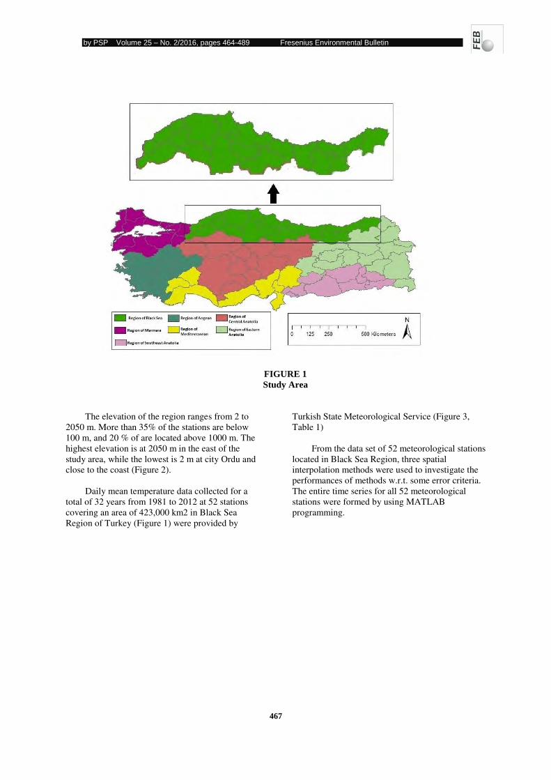
by PSP Volume 25 – No. 2/2016, pages 464-489 Fresenius Environmental Bulletin
467
FIGURE 1
Study Area
The elevation of the region ranges from 2 to
2050 m. More than 35% of the stations are below
100 m, and 20 % of are located above 1000 m. The
highest elevation is at 2050 m in the east of the
study area, while the lowest is 2 m at city Ordu and
close to the coast (Figure 2).
Daily mean temperature data collected for a
total of 32 years from 1981 to 2012 at 52 stations
covering an area of 423,000 km2 in Black Sea
Region of Turkey (Figure 1) were provided by
Turkish State Meteorological Service (Figure 3,
Table 1)
From the data set of 52 meteorological stations
located in Black Sea Region, three spatial
interpolation methods were used to investigate the
performances of methods w.r.t. some error criteria.
The entire time series for all 52 meteorological
stations were formed by using MATLAB
programming.
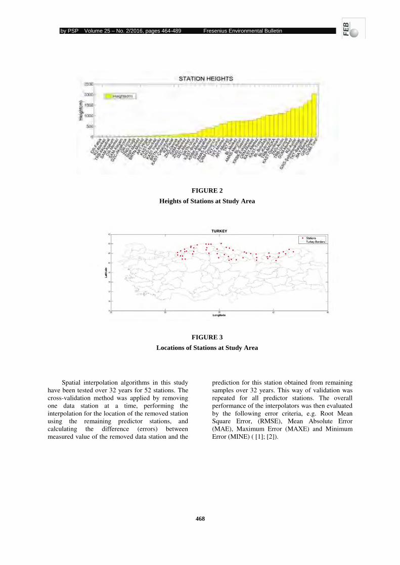
by PSP Volume 25 – No. 2/2016, pages 464-489 Fresenius Environmental Bulletin
468
FIGURE 2
Heights of Stations at Study Area
FIGURE 3
Locations of Stations at Study Area
Spatial interpolation algorithms in this study
have been tested over 32 years for 52 stations. The
cross-validation method was applied by removing
one data station at a time, performing the
interpolation for the location of the removed station
using the remaining predictor stations, and
calculating the difference (errors) between
measured value of the removed data station and the
prediction for this station obtained from remaining
samples over 32 years. This way of validation was
repeated for all predictor stations. The overall
performance of the interpolators was then evaluated
by the following error criteria, e.g. Root Mean
Square Error, (RMSE), Mean Absolute Error
(MAE), Maximum Error (MAXE) and Minimum
Error (MINE) ( [1]; [2]).
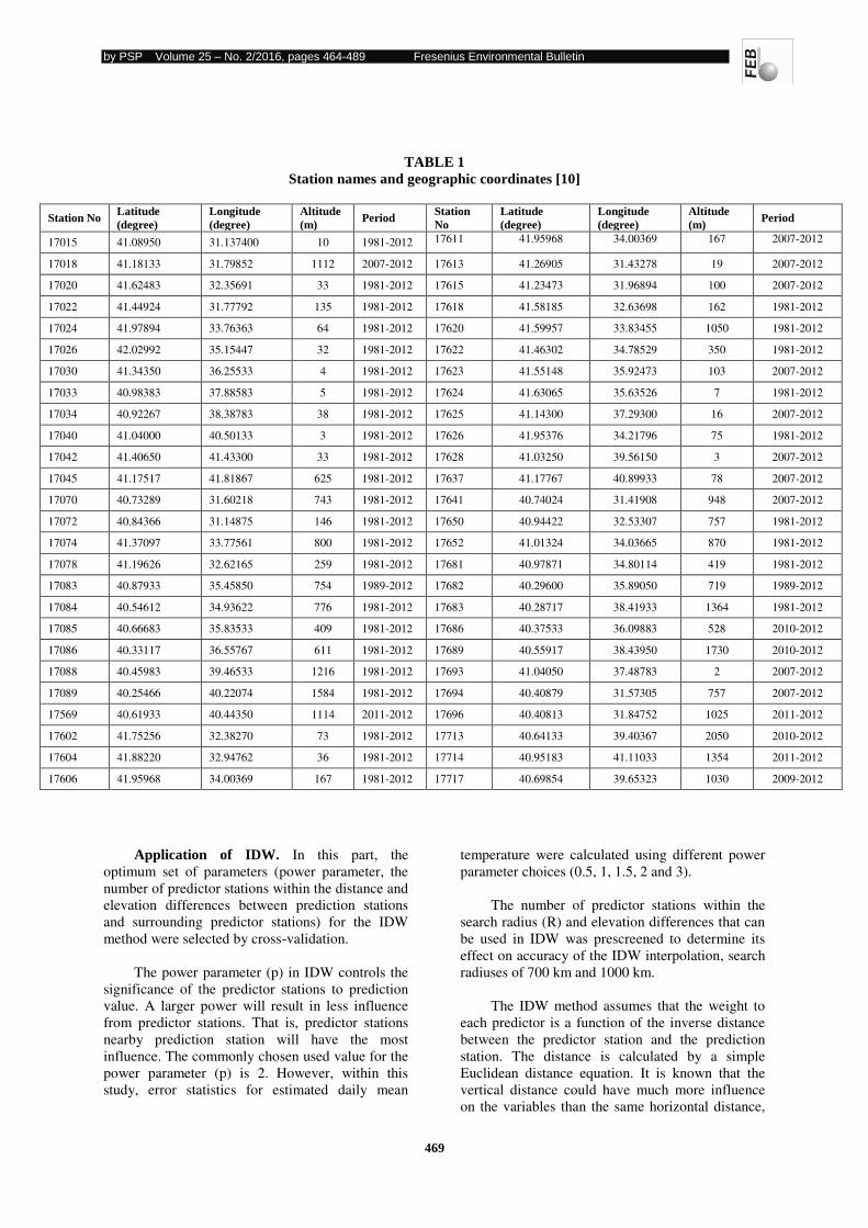
by PSP Volume 25 – No. 2/2016, pages 464-489 Fresenius Environmental Bulletin
469
TABLE 1
Station names and geographic coordinates [10]
Station No Latitude
(degree)
Longitude
(degree)
Altitude
(m) Period
Station
No
Latitude
(degree)
Longitude
(degree)
Altitude
(m) Period
17015 41.08950 31.137400 10 1981-2012 17611 41.95968 34.00369 167 2007-2012
17018 41.18133 31.79852 1112 2007-2012 17613 41.26905 31.43278 19 2007-2012
17020 41.62483 32.35691 33 1981-2012 17615 41.23473 31.96894 100 2007-2012
17022 41.44924 31.77792 135 1981-2012 17618 41.58185 32.63698 162 1981-2012
17024 41.97894 33.76363 64 1981-2012 17620 41.59957 33.83455 1050 1981-2012
17026 42.02992 35.15447 32 1981-2012 17622 41.46302 34.78529 350 1981-2012
17030 41.34350 36.25533 4 1981-2012 17623 41.55148 35.92473 103 2007-2012
17033 40.98383 37.88583 5 1981-2012 17624 41.63065 35.63526 7 1981-2012
17034 40.92267 38.38783 38 1981-2012 17625 41.14300 37.29300 16 2007-2012
17040 41.04000 40.50133 3 1981-2012 17626 41.95376 34.21796 75 1981-2012
17042 41.40650 41.43300 33 1981-2012 17628 41.03250 39.56150 3 2007-2012
17045 41.17517 41.81867 625 1981-2012 17637 41.17767 40.89933 78 2007-2012
17070 40.73289 31.60218 743 1981-2012 17641 40.74024 31.41908 948 2007-2012
17072 40.84366 31.14875 146 1981-2012 17650 40.94422 32.53307 757 1981-2012
17074 41.37097 33.77561 800 1981-2012 17652 41.01324 34.03665 870 1981-2012
17078 41.19626 32.62165 259 1981-2012 17681 40.97871 34.80114 419 1981-2012
17083 40.87933 35.45850 754 1989-2012 17682 40.29600 35.89050 719 1989-2012
17084 40.54612 34.93622 776 1981-2012 17683 40.28717 38.41933 1364 1981-2012
17085 40.66683 35.83533 409 1981-2012 17686 40.37533 36.09883 528 2010-2012
17086 40.33117 36.55767 611 1981-2012 17689 40.55917 38.43950 1730 2010-2012
17088 40.45983 39.46533 1216 1981-2012 17693 41.04050 37.48783 2 2007-2012
17089 40.25466 40.22074 1584 1981-2012 17694 40.40879 31.57305 757 2007-2012
17569 40.61933 40.44350 1114 2011-2012 17696 40.40813 31.84752 1025 2011-2012
17602 41.75256 32.38270 73 1981-2012 17713 40.64133 39.40367 2050 2010-2012
17604 41.88220 32.94762 36 1981-2012 17714 40.95183 41.11033 1354 2011-2012
17606 41.95968 34.00369 167 1981-2012 17717 40.69854 39.65323 1030 2009-2012
Application of IDW. In this part, the
optimum set of parameters (power parameter, the
number of predictor stations within the distance and
elevation differences between prediction stations
and surrounding predictor stations) for the IDW
method were selected by cross-validation.
The power parameter (p) in IDW controls the
significance of the predictor stations to prediction
value. A larger power will result in less influence
from predictor stations. That is, predictor stations
nearby prediction station will have the most
influence. The commonly chosen used value for the
power parameter (p) is 2. However, within this
study, error statistics for estimated daily mean
temperature were calculated using different power
parameter choices (0.5, 1, 1.5, 2 and 3).
The number of predictor stations within the
search radius (R) and elevation differences that can
be used in IDW was prescreened to determine its
effect on accuracy of the IDW interpolation, search
radiuses of 700 km and 1000 km.
The IDW method assumes that the weight to
each predictor is a function of the inverse distance
between the predictor station and the prediction
station. The distance is calculated by a simple
Euclidean distance equation. It is known that the
vertical distance could have much more influence
on the variables than the same horizontal distance,
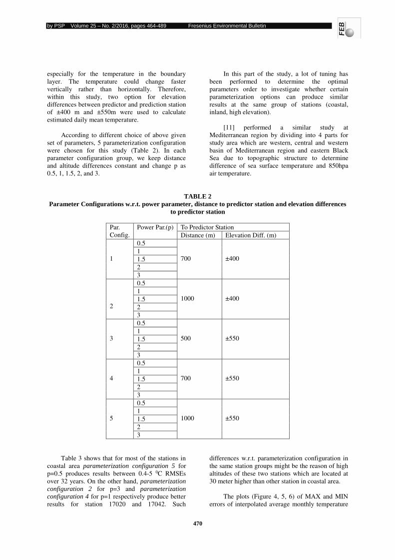
by PSP Volume 25 – No. 2/2016, pages 464-489 Fresenius Environmental Bulletin
470
especially for the temperature in the boundary
layer. The temperature could change faster
vertically rather than horizontally. Therefore,
within this study, two option for elevation
differences between predictor and prediction station
of ±400 m and ±550m were used to calculate
estimated daily mean temperature.
According to different choice of above given
set of parameters, 5 parameterization configuration
were chosen for this study (Table 2). In each
parameter configuration group, we keep distance
and altitude differences constant and change p as
0.5, 1, 1.5, 2, and 3.
In this part of the study, a lot of tuning has
been performed to determine the optimal
parameters order to investigate whether certain
parameterization options can produce similar
results at the same group of stations (coastal,
inland, high elevation).
[11] performed a similar study at
Mediterranean region by dividing into 4 parts for
study area which are western, central and western
basin of Mediterranean region and eastern Black
Sea due to topographic structure to determine
difference of sea surface temperature and 850hpa
air temperature.
TABLE 2
Parameter Configurations w.r.t. power parameter, distance to predictor station and elevation differences
to predictor station
Par.
Config.
Power Par.(p) To Predictor Station
Distance (m) Elevation Diff. (m)
1
0.5
700
±400 1
1.5
2
3
2
0.5
1000
±400 1
1.5
2
3
3
0.5
500
±550 1
1.5
2
3
4
0.5
700
±550 1
1.5
2
3
5
0.5
1000
±550 1
1.5
2
3
Table 3 shows that for most of the stations in
coastal area parameterization configuration 5 for
p=0.5 produces results between 0.4-5 0C RMSEs
over 32 years. On the other hand, parameterization
configuration 2 for p=3 and parameterization
configuration 4 for p=1 respectively produce better
results for station 17020 and 17042. Such
differences w.r.t. parameterization configuration in
the same station groups might be the reason of high
altitudes of these two stations which are located at
30 meter higher than other station in coastal area.
The plots (Figure 4, 5, 6) of MAX and MIN
errors of interpolated average monthly temperature
by PSP Volume 25 – No. 2/2016, pages 464-489 Fresenius Environmental Bulletin
471
presents a comparison for seven coastal stations in
years 1990, 2002, 2011. Focusing on the results for
17020 as highest elevation station among coastal
stations (33m) and lowest elevation station 17040
(3 m) throughout the years 1990, 2002 and 2011,
parameterization configuration 5 of IDW
performance (p=0.5) increased at station 17020
with smaller MAXE and MIN interpolation error
and decreased at station 17040 with larger errors
(Figure 4). Above all, the interpolation errors vary
seasonaly for all coastal stations. The largest
interpolation errors occur for highest temperatures
in summer seasons.
Figure 5 illustrates that the performance of
parameterization configuration 2(p=3) for IDW.
Interpolation errors indicates that seasonal
differences are similar for all coastal stations and
the improvement in interpolation errors is greatest
in winter seasons.
Parameterization configuration 4 (p=1) for
IDW (Figure 6) shows generally larger
interpolation errors (MAXE between 2-20°C and
MIN between 0-15°C) than other parameter
configurations (MAXE between 2-16°C and MIN
between 0-12°C) (Figure 4 and Figure 5). Table 4
indicates that stations 17681, 17070, 17083, 17084
and 17074 in inland area produce better results over
32 years for parameterization configuration 1 and
parameter configuration 2 with various power
parameters (p=0.5, 1, 2 and 3) between 0.3-4°C
RMSEs over 32 years.
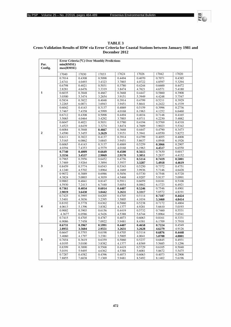
by PSP Volume 25 – No. 2/2016, pages 464-489 Fresenius Environmental Bulletin
472
TABLE 3
Cross-Validation Results of IDW via Error Criteria for Coastal Stations between January 1981 and
December 2012
Par.
Config.
Error Criteria (0C) Over Monthly Predictions
min(RMSE)
max(RMSE)
17040 17030 17033 17624 17026 17042 17020
1
0.7014
2.6741
0.4308
4.0493
0.5098
3.4323
0.4494
3.7003
0.4070
4.0722
0.7071
4.8597
0.4385
5.3294
0.6798
2.8281
0.4021
4.6476
0.5031
3.3319
0.3780
3.8474
0.4244
4.7621
0.6600
4.6571
0.4472
5.4180
0.6035
3.0300
0.3848
5.3474
0.4667
3.2654
0.3668
3.9151
0.4447
5.3949
0.5860
4.4248
0.3908
5.7547
0.5834
3.2265
0.3822
6.0871
0.4048
3.6943
0.3914
3.9451
0.4799
5.8641
0.5211
4.2422
0.3929
6.1539
0.6042
3.7467
0.4143
7.4358
0.3137
4.5999
0.4069
4.0168
0.5159
6.1963
0.3996
4.1252
0.2736
6.6460
2
0.6712
3.5065
0.4308
4.0464
0.5098
3.4292
0.4494
3.7003
0.4034
4.0711
0.7148
4.2230
0.4165
5.4882
0.6047
3.4523
0.4021
4.6439
0.5031
3.3274
0.3780
3.8474
0.4194
4.7609
0.5769
3.9023
0.4318
5.5342
0.6084
3.4590
0.3848
5.3455 0.4667
3.2629
0.3668
3.9151
0.4447
5.3941
0.4790
4.0550
0.3473
5.8272
0.6111
3.5165
0.3822
6.0862
0.4137
3.6845
0.3914
3.9451
0.4799
5.8637
0.4055
4.0948
0.4008
6.1926
0.6065
4.0394
0.4143
7.4353
0.3137
4.5579
0.4069
4.0168
0.5259
6.1963 0.3066
4.4517
0.2907
6.6550
3
0.7740
3.3556
0.4009
3.4537
0.6649
2.9069
0.4500
2.9170
0.5615
3.3051
0.7630
5.2837
0.6017
4.4152
0.7965
3.7469
0.3956
3.9264
0.6452
3.3894
0.4756
3.5937
0.5114
3.3287
0.7419
5.4918
0.5001
4.4619
0.8459
4.1240
0.3774
4.5702
0.6543
3.8964
0.5343
4.1669
0.5250
3.9936
0.7372
5.7146
0.4751
4.6428
0 9072
4.3824
0.3889
5.0003
0.6986
4.3039
0.5856
4.5468
0.5730
4.9207
0.7548
5.9137
0.5720
5.0991
0.9882
4.5930
0.4841
7.2413
0.8147
6.7440
0.5911
5.6054
0.6059
8.0862
0.8181
6.1723
0.5108
6.4921
4
0.7361
2.9019
0.4034
3.6430
0.6014
3.0442
0.4407
3.2631
0.5246
3.3317
0.7546
5.0572
0.4901
4.8191
0.7425
3.5401
0.3995
4.3036
0.6205
3.2395
0.4705
3.5005
0.5114
4.1034
0.7187
5.3460
0.4424
4.8414
0.8192
4.0613
0.3778
5.1396
0.6362
3.8382
0.5060
4.1377
0.5238
4.9281
0.7172
5.6610
0.4804
5.0193
0.9002
4.3677
0.3903
6.0586
0.6156
4.5426
0.4419
4.5388
0.5732
5.6744
0.7460
5.8964
0.5531
5.6541
0.7415
6.9086
0.4705
7.7458
0.4787
7.0922
0.4073
5.9481
0.6063
8.4381
0.8161
6.1709
0.3331
5.7918
5
0.6731
2.8955
0.3967
3.5604
0.5991
2.9551
0.4407
3.2631
0.4658
3.2628
0.7224
4.6279
0.4549
4.9126
0.6647
3.4060
0.3793
4.1797
0.6198
3.2381
0.4705
3.5005
0.5114
4.0041
0.6876
5.0788
0.4448
4.8801
0.7654
4.0195
0.3619
5.0100
0.6359
3.8382
0.5060
4.1377
0.5237
4.8369
0.6845
5.5685
0.4931
5.1296
0.8399
5.0191
0.3890
5.9495
0.5568
4.6362
0.4419
4.5388
0.5729
5.6081
0.6105
5.8672
0.5040
5.5475
0.7287
7.8855
0.4582
7.6838
0.4396
7.1369
0.4073
5.9481
0.6063
8.5492
0.4073
8.1402
0.2908
5.6196
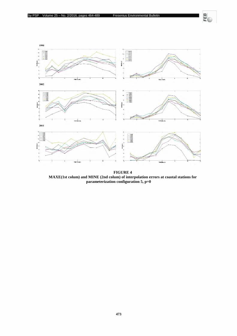
by PSP Volume 25 – No. 2/2016, pages 464-489 Fresenius Environmental Bulletin
473
FIGURE 4
MAXE(1st colum) and MINE (2nd colum) of interpolation errors at coastal stations for
parameterization configuration 5, p=0
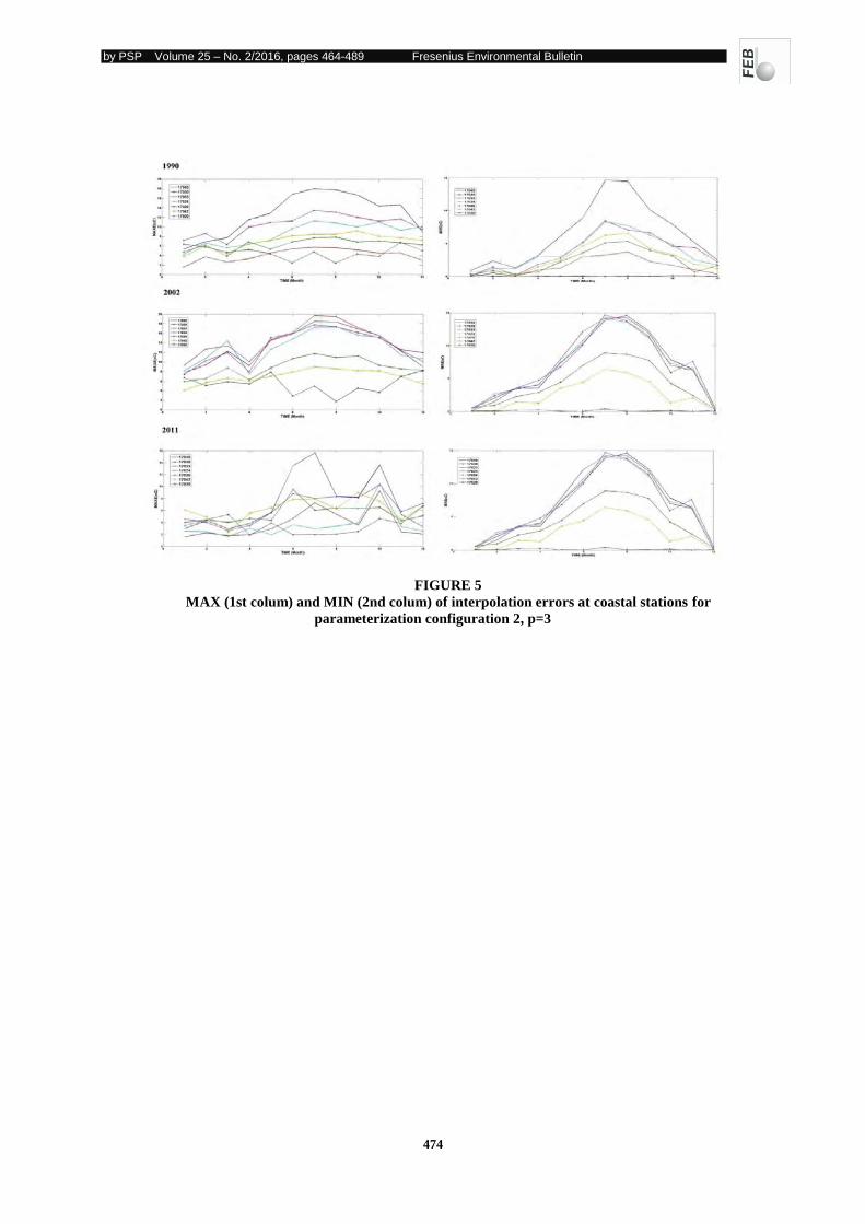
by PSP Volume 25 – No. 2/2016, pages 464-489 Fresenius Environmental Bulletin
474
FIGURE 5
MAX (1st colum) and MIN (2nd colum) of interpolation errors at coastal stations for
parameterization configuration 2, p=3
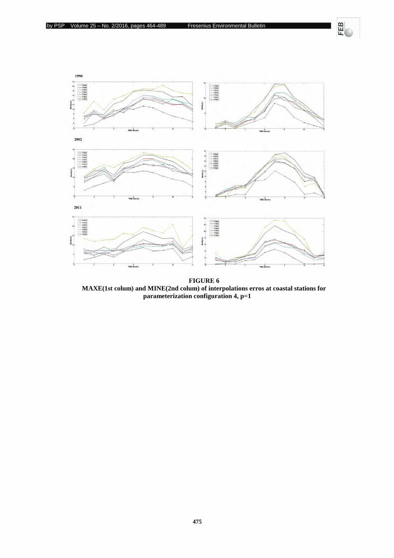
by PSP Volume 25 – No. 2/2016, pages 464-489 Fresenius Environmental Bulletin
475
FIGURE 6
MAXE(1st colum) and MINE(2nd colum) of interpolations erros at coastal stations for
parameterization configuration 4, p=1
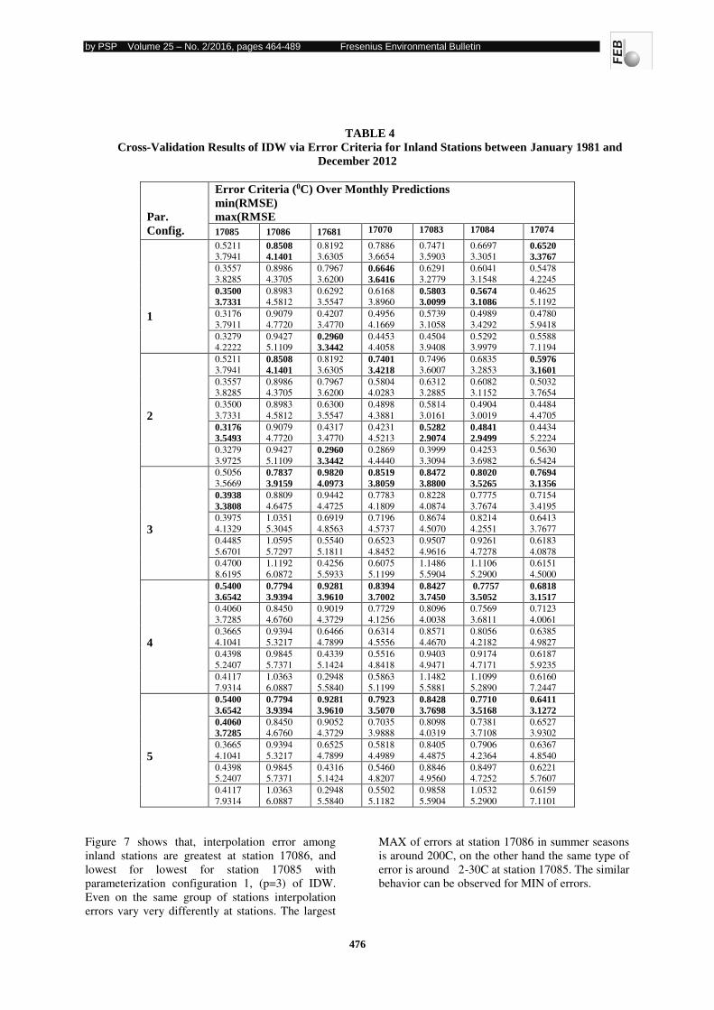
by PSP Volume 25 – No. 2/2016, pages 464-489 Fresenius Environmental Bulletin
476
TABLE 4
Cross-Validation Results of IDW via Error Criteria for Inland Stations between January 1981 and
December 2012
Par.
Config.
Error Criteria (0C) Over Monthly Predictions
min(RMSE)
max(RMSE
17085 17086 17681 17070 17083 17084 17074
1
0.5211
3.7941 0.8508
4.1401
0.8192
3.6305
0.7886
3.6654
0.7471
3.5903
0.6697
3.3051 0.6520
3.3767
0.3557
3.8285
0.8986
4.3705
0.7967
3.6200
0.6646
3.6416
0.6291
3.2779
0.6041
3.1548
0.5478
4.2245
0.3500
3.7331
0.8983
4.5812
0.6292
3.5547
0.6168
3.8960 0.5803
3.0099
0.5674
3.1086
0.4625
5.1192
0.3176
3.7911
0.9079
4.7720
0.4207
3.4770
0.4956
4.1669
0.5739
3.1058
0.4989
3.4292
0.4780
5.9418
0.3279
4.2222
0.9427
5.1109 0.2960
3.3442
0.4453
4.4058
0.4504
3.9408
0.5292
3.9979
0.5588
7.1194
2
0.5211
3.7941
0.8508
4.1401
0.8192
3.6305
0.7401
3.4218
0.7496
3.6007
0.6835
3.2853
0.5976
3.1601
0.3557
3.8285
0.8986
4.3705
0.7967
3.6200
0.5804
4.0283
0.6312
3.2885
0.6082
3.1152
0.5032
3.7654
0.3500
3.7331
0.8983
4.5812
0.6300
3.5547
0.4898
4.3881
0.5814
3.0161
0.4904
3.0019
0.4484
4.4705
0.3176
3.5493
0.9079
4.7720
0.4317
3.4770
0.4231
4.5213 0.5282
2.9074
0.4841
2.9499
0.4434
5.2224
0.3279
3.9725
0.9427
5.1109
0.2960
3.3442
0.2869
4.4440
0.3999
3.3094
0.4253
3.6982
0.5630
6.5424
3
0.5056
3.5669
0.7837
3.9159
0.9820
4.0973
0.8519
3.8059
0.8472
3.8800
0.8020
3.5265
0.7694
3.1356
0.3938
3.3808
0.8809
4.6475
0.9442
4.4725
0.7783
4.1809
0.8228
4.0874
0.7775
3.7674
0.7154
3.4195
0.3975
4.1329
1.0351
5.3045
0.6919
4.8563
0.7196
4.5737
0.8674
4.5070
0.8214
4.2551
0.6413
3.7677
0.4485
5.6701
1.0595
5.7297
0.5540
5.1811
0.6523
4.8452
0.9507
4.9616
0.9261
4.7278
0.6183
4.0878
0.4700
8.6195
1.1192
6.0872
0.4256
5.5933
0.6075
5.1199
1.1486
5.5904
1.1106
5.2900
0.6151
4.5000
4
0.5400
3.6542
0.7794
3.9394
0.9281
3.9610
0.8394
3.7002
0.8427
3.7450
0.7757
3.5052
0.6818
3.1517
0.4060
3.7285
0.8450
4.6760
0.9019
4.3729
0.7729
4.1256
0.8096
4.0038
0.7569
3.6811
0.7123
4.0061
0.3665
4.1041
0.9394
5.3217
0.6466
4.7899
0.6314
4.5556
0.8571
4.4670
0.8056
4.2182
0.6385
4.9827
0.4398
5.2407
0.9845
5.7371
0.4339
5.1424
0.5516
4.8418
0.9403
4.9471
0.9174
4.7171
0.6187
5.9235
0.4117
7.9314
1.0363
6.0887
0.2948
5.5840
0.5863
5.1199
1.1482
5.5881
1.1099
5.2890
0.6160
7.2447
5
0.5400
3.6542
0.7794
3.9394
0.9281
3.9610
0.7923
3.5070
0.8428
3.7698
0.7710
3.5168
0.6411
3.1272
0.4060
3.7285
0.8450
4.6760
0.9052
4.3729
0.7035
3.9888
0.8098
4.0319
0.7381
3.7108
0.6527
3.9302
0.3665
4.1041
0.9394
5.3217
0.6525
4.7899
0.5818
4.4989
0.8405
4.4875
0.7906
4.2364
0.6367
4.8540
0.4398
5.2407
0.9845
5.7371
0.4316
5.1424
0.5460
4.8207
0.8846
4.9560
0.8497
4.7252
0.6221
5.7607
0.4117
7.9314
1.0363
6.0887
0.2948
5.5840
0.5502
5.1182
0.9858
5.5904
1.0532
5.2900
0.6159
7.1101
Figure 7 shows that, interpolation error among
inland stations are greatest at station 17086, and
lowest for lowest for station 17085 with
parameterization configuration 1, (p=3) of IDW.
Even on the same group of stations interpolation
errors vary very differently at stations. The largest
MAX of errors at station 17086 in summer seasons
is around 200C, on the other hand the same type of
error is around 2-30C at station 17085. The similar
behavior can be observed for MIN of errors.
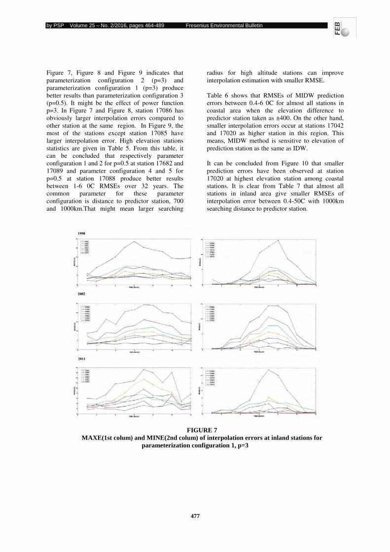
by PSP Volume 25 – No. 2/2016, pages 464-489 Fresenius Environmental Bulletin
477
Figure 7, Figure 8 and Figure 9 indicates that
parameterization configuration 2 (p=3) and
parameterization configuration 1 (p=3) produce
better results than parameterization configuration 3
(p=0.5). It might be the effect of power function
p=3. In Figure 7 and Figure 8, station 17086 has
obviously larger interpolation errors compared to
other station at the same region. In Figure 9, the
most of the stations except station 17085 have
larger interpolation error. High elevation stations
statistics are given in Table 5. From this table, it
can be concluded that respectively parameter
configuration 1 and 2 for p=0.5 at station 17682 and
17089 and parameter configuration 4 and 5 for
p=0.5 at station 17088 produce better results
between 1-6 0C RMSEs over 32 years. The
common parameter for these parameter
configuration is distance to predictor station, 700
and 1000km.That might mean larger searching
radius for high altitude stations can improve
interpolation estimation with smaller RMSE.
Table 6 shows that RMSEs of MIDW prediction
errors between 0.4-6 0C for almost all stations in
coastal area when the elevation difference to
predictor station taken as ±400. On the other hand,
smaller interpolation errors occur at stations 17042
and 17020 as higher station in this region. This
means, MIDW method is sensitive to elevation of
prediction station as the same as IDW.
It can be concluded from Figure 10 that smaller
prediction errors have been observed at station
17020 at highest elevation station among coastal
stations. It is clear from Table 7 that almost all
stations in inland area give smaller RMSEs of
interpolation error between 0.4-50C with 1000km
searching distance to predictor station.
FIGURE 7
MAXE(1st colum) and MINE(2nd colum) of interpolation errors at inland stations for
parameterization configuration 1, p=3
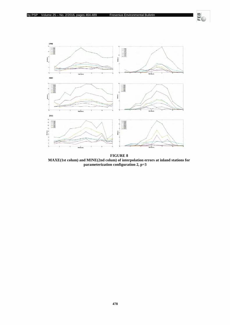
by PSP Volume 25 – No. 2/2016, pages 464-489 Fresenius Environmental Bulletin
478
FIGURE 8
MAXE(1st colum) and MINE(2nd colum) of interpolation errors at inland stations for
parameterization configuration 2, p=3
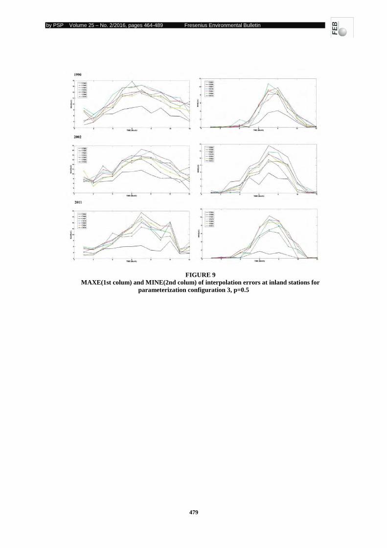
by PSP Volume 25 – No. 2/2016, pages 464-489 Fresenius Environmental Bulletin
479
FIGURE 9
MAXE(1st colum) and MINE(2nd colum) of interpolation errors at inland stations for
parameterization configuration 3, p=0.5
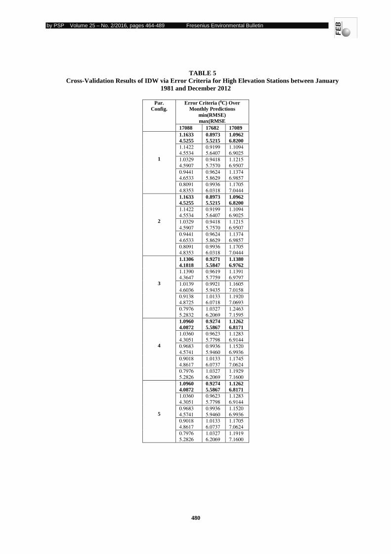
by PSP Volume 25 – No. 2/2016, pages 464-489 Fresenius Environmental Bulletin
480
TABLE 5
Cross-Validation Results of IDW via Error Criteria for High Elevation Stations between January
1981 and December 2012
Par.
Config.
Error Criteria (0C) Over
Monthly Predictions
min(RMSE)
max(RMSE
17088 17682 17089
1
1.1633
4.5255
0.8973
5.5215
1.0962
6.8200
1.1422
4.5534
0.9199
5.6407
1.1094
6.9025
1.0329
4.5907
0.9418
5.7570
1.1215
6.9507
0.9441
4.6533
0.9624
5.8629
1.1374
6.9857
0.8091
4.8353
0.9936
6.0318
1.1705
7.0444
2
1.1633
4.5255
0.8973
5.5215
1.0962
6.8200
1.1422
4.5534
0.9199
5.6407
1.1094
6.9025
1.0329
4.5907
0.9418
5.7570
1.1215
6.9507
0.9441
4.6533
0.9624
5.8629
1.1374
6.9857
0.8091
4.8353
0.9936
6.0318
1.1705
7.0444
3
1.1306
4.1818
0.9271
5.5847
1.1380
6.9762
1.1390
4.3647
0.9619
5.7759
1.1391
6.9797
1.0139
4.6036
0.9921
5.9435
1.1605
7.0158
0.9138
4.8725
1.0133
6.0718
1.1920
7.0693
0.7976
5.2832
1.0327
6.2069
1.2463
7.1595
4
1.0960
4.0872
0.9274
5.5867
1.1262
6.8171
1.0360
4.3051
0.9623
5.7798
1.1283
6.9144
0.9683
4.5741
0.9936
5.9460
1.1520
6.9936
0.9018
4.8617
1.0133
6.0737
1.1745
7.0624
0.7976
5.2826
1.0327
6.2069
1.1929
7.1600
5
1.0960
4.0872
0.9274
5.5867
1.1262
6.8171
1.0360
4.3051
0.9623
5.7798
1.1283
6.9144
0.9683
4.5741
0.9936
5.9460
1.1520
6.9936
0.9018
4.8617
1.0133
6.0737
1.1705
7.0624
0.7976
5.2826
1.0327
6.2069
1.1919
7.1600
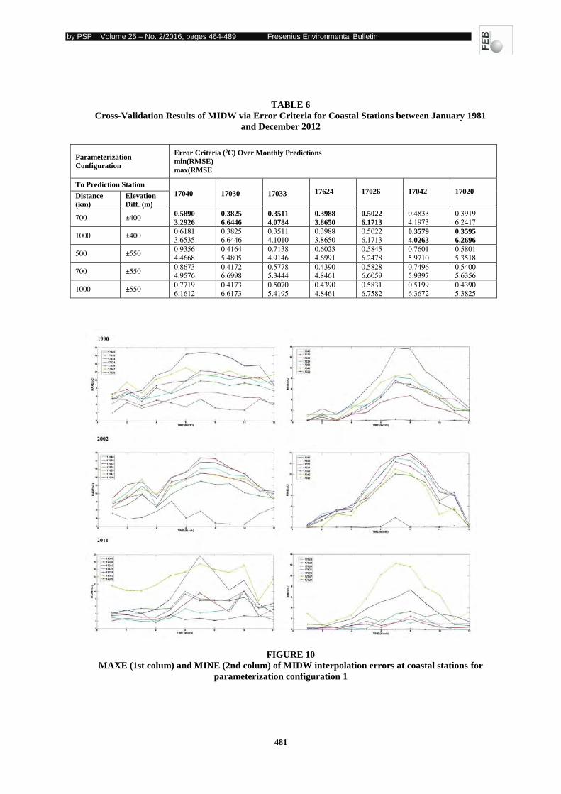
by PSP Volume 25 – No. 2/2016, pages 464-489 Fresenius Environmental Bulletin
481
TABLE 6
Cross-Validation Results of MIDW via Error Criteria for Coastal Stations between January 1981
and December 2012
FIGURE 10
MAXE (1st colum) and MINE (2nd colum) of MIDW interpolation errors at coastal stations for
parameterization configuration 1
Parameterization
Configuration
Error Criteria (0C) Over Monthly Predictions
min(RMSE)
max(RMSE
To Prediction Station
17040 17030 17033
17624
17026
17042
17020 Distance
(km)
Elevation
Diff. (m)
700 ±400 0.5890
3.2926
0.3825
6.6446
0.3511
4.0784
0.3988
3.8650
0.5022
6.1713
0.4833
4.1973
0.3919
6.2417
1000 ±400 0.6181
3.6535
0.3825
6.6446
0.3511
4.1010
0.3988
3.8650
0.5022
6.1713 0.3579
4.0263
0.3595
6.2696
500 ±550 0 9356
4.4668
0.4164
5.4805
0.7138
4.9146
0.6023
4.6991
0.5845
6.2478
0.7601
5.9710
0.5801
5.3518
700 ±550 0.8673
4.9576
0.4172
6.6998
0.5778
5.3444
0.4390
4.8461
0.5828
6.6059
0.7496
5.9397
0.5400
5.6356
1000 ±550 0.7719
6.1612
0.4173
6.6173
0.5070
5.4195
0.4390
4.8461
0.5831
6.7582
0.5199
6.3672
0.4390
5.3825
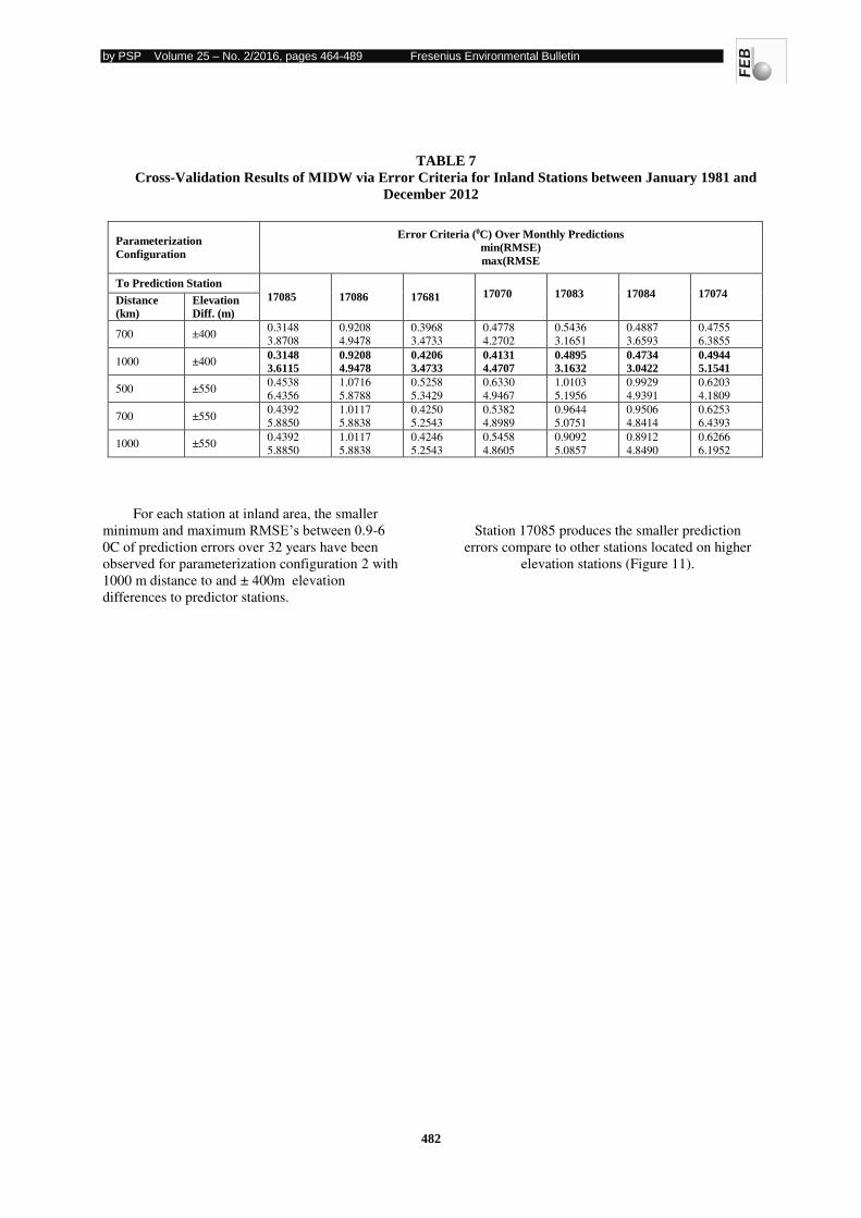
by PSP Volume 25 – No. 2/2016, pages 464-489 Fresenius Environmental Bulletin
482
TABLE 7
Cross-Validation Results of MIDW via Error Criteria for Inland Stations between January 1981 and
December 2012
For each station at inland area, the smaller
minimum and maximum RMSE’s between 0.9-6
0C of prediction errors over 32 years have been
observed for parameterization configuration 2 with
1000 m distance to and ± 400m elevation
differences to predictor stations.
Station 17085 produces the smaller prediction
errors compare to other stations located on higher
elevation stations (Figure 11).
Parameterization
Configuration
Error Criteria (0C) Over Monthly Predictions
min(RMSE)
max(RMSE
To Prediction Station
17085 17086 17681
17070
17083
17084
17074 Distance
(km)
Elevation
Diff. (m)
700 ±400 0.3148
3.8708
0.9208
4.9478
0.3968
3.4733
0.4778
4.2702
0.5436
3.1651
0.4887
3.6593
0.4755
6.3855
1000 ±400 0.3148
3.6115
0.9208
4.9478
0.4206
3.4733
0.4131
4.4707
0.4895
3.1632
0.4734
3.0422
0.4944
5.1541
500 ±550 0.4538
6.4356
1.0716
5.8788
0.5258
5.3429
0.6330
4.9467
1.0103
5.1956
0.9929
4.9391
0.6203
4.1809
700 ±550 0.4392
5.8850
1.0117
5.8838
0.4250
5.2543
0.5382
4.8989
0.9644
5.0751
0.9506
4.8414
0.6253
6.4393
1000 ±550 0.4392
5.8850
1.0117
5.8838
0.4246
5.2543
0.5458
4.8605
0.9092
5.0857
0.8912
4.8490
0.6266
6.1952
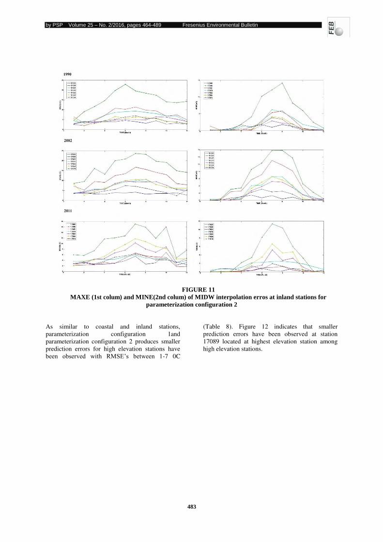
by PSP Volume 25 – No. 2/2016, pages 464-489 Fresenius Environmental Bulletin
483
FIGURE 11
MAXE (1st colum) and MINE(2nd colum) of MIDW interpolation erros at inland stations for
parameterization configuration 2
As similar to coastal and inland stations,
parameterization configuration 1and
parameterization configuration 2 produces smaller
prediction errors for high elevation stations have
been observed with RMSE’s between 1-7 0C
(Table 8). Figure 12 indicates that smaller
prediction errors have been observed at station
17089 located at highest elevation station among
high elevation stations.
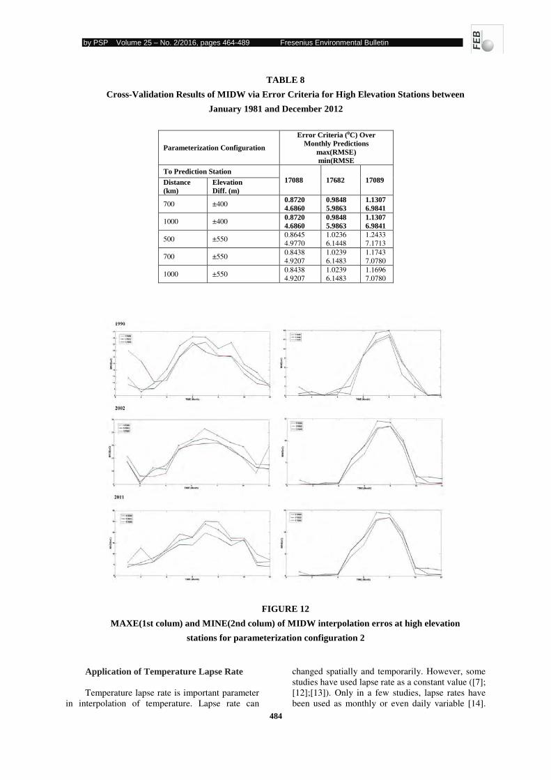
by PSP Volume 25 – No. 2/2016, pages 464-489 Fresenius Environmental Bulletin
484
TABLE 8
Cross-Validation Results of MIDW via Error Criteria for High Elevation Stations between
January 1981 and December 2012
Parameterization Configuration
Error Criteria (0C) Over
Monthly Predictions
max(RMSE)
min(RMSE
To Prediction Station
17088 17682 17089 Distance
(km)
Elevation
Diff. (m)
700 ±400 0.8720
4.6860
0.9848
5.9863
1.1307
6.9841
1000 ±400 0.8720
4.6860
0.9848
5.9863
1.1307
6.9841
500 ±550 0.8645
4.9770
1.0236
6.1448
1.2433
7.1713
700 ±550 0.8438
4.9207
1.0239
6.1483
1.1743
7.0780
1000 ±550 0.8438
4.9207
1.0239
6.1483
1.1696
7.0780
FIGURE 12
MAXE(1st colum) and MINE(2nd colum) of MIDW interpolation erros at high elevation
stations for parameterization configuration 2
Application of Temperature Lapse Rate
Temperature lapse rate is important parameter
in interpolation of temperature. Lapse rate can
changed spatially and temporarily. However, some
studies have used lapse rate as a constant value ([7];
[12];[13]). Only in a few studies, lapse rates have
been used as monthly or even daily variable [14].
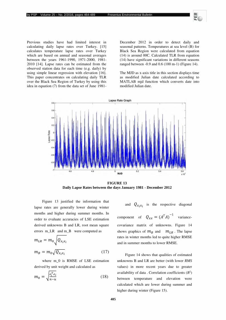
by PSP Volume 25 – No. 2/2016, pages 464-489 Fresenius Environmental Bulletin
485
Previous studies have had limited interest in
calculating daily lapse rates over Turkey. [15]
calculates temperature lapse rates over Turkey
which are based on annual and seasonal averages
between the years 1961-1990, 1971-2000, 1981-
2010 [14]. Lapse rates can be estimated from the
observed station data for each time (e.g. daily) by
using simple linear regression with elevation [16].
This paper concentrates on calculating daily TLR
over the Black Sea Region of Turkey by using this
idea in equation (7) from the data set of June 1981-
December 2012 in order to detect daily and
seasonal patterns. Temperatures at sea level (B) for
Black Sea Region were calculated from equation
(14) is around 00C. Calculated TLR from equation
(14) have significant variations in different seasons
ranged between -0.9 and 0.6 (100 m-1) (Figure 14).
The MJD as x-axis title in this section displays time
as modified Julian date calculated according to
MATLAB mjd function which converts date into
modified Julian date.
FIGURE 13
Daily Lapse Rates between the days January 1981 - December 2012
Figure 13 justified the information that
lapse rates are generally lower during winter
months and higher during summer months. In
order to evaluate accuracies of LSE estimation
derived unknowns B and LR, root mean square
errors m_LR and m_B were computed as
�� = √ ���� � = √ ���� (17)
where m_0 is RMSE of LSE estimation
derived by unit weight and calculated as = √������−� (18)
and ���� is the respective diagonal
component of �� = � − variance-
covariance matrix of unknowns. Figure 14
shows graphics of � and �� . The lapse
rates in winter months led to quite higher RMSE
and in summer months to lower RMSE.
Figure 14 shows that qualities of estimated
unknowns B and LR are better (with lower RMS
values) in more recent years due to greater
availability of data . Correlation coefficients (R2)
between temperature and elevation were
calculated which are lower during summer and
higher during winter (Figure 15).
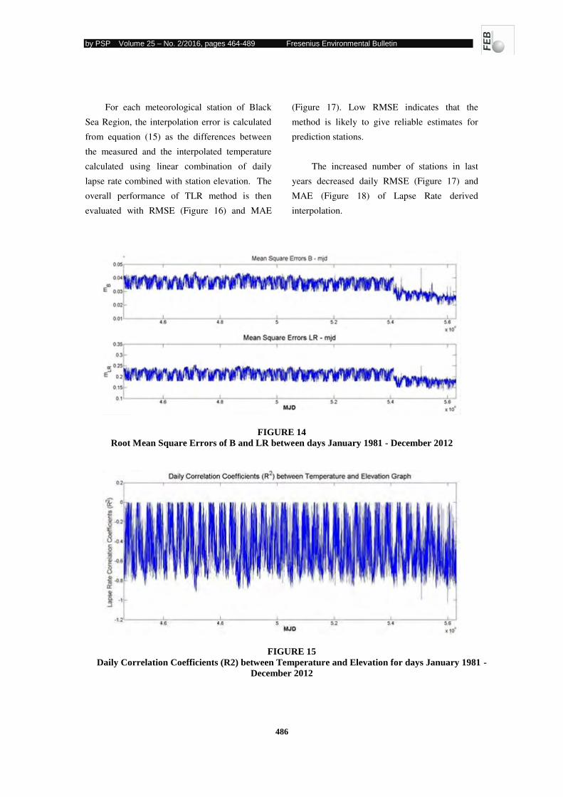
by PSP Volume 25 – No. 2/2016, pages 464-489 Fresenius Environmental Bulletin
486
For each meteorological station of Black
Sea Region, the interpolation error is calculated
from equation (15) as the differences between
the measured and the interpolated temperature
calculated using linear combination of daily
lapse rate combined with station elevation. The
overall performance of TLR method is then
evaluated with RMSE (Figure 16) and MAE
(Figure 17). Low RMSE indicates that the
method is likely to give reliable estimates for
prediction stations.
The increased number of stations in last
years decreased daily RMSE (Figure 17) and
MAE (Figure 18) of Lapse Rate derived
interpolation.
FIGURE 14
Root Mean Square Errors of B and LR between days January 1981 - December 2012
FIGURE 15
Daily Correlation Coefficients (R2) between Temperature and Elevation for days January 1981 -
December 2012
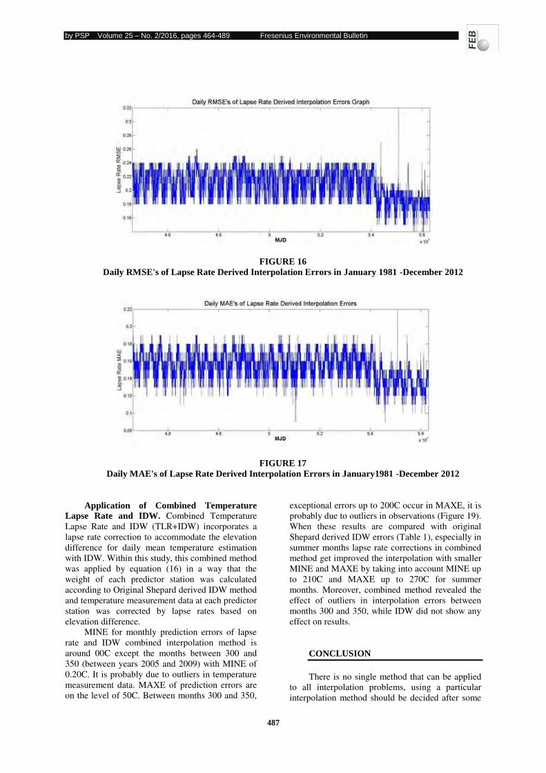
by PSP Volume 25 – No. 2/2016, pages 464-489 Fresenius Environmental Bulletin
487
FIGURE 16
Daily RMSE's of Lapse Rate Derived Interpolation Errors in January 1981 -December 2012
FIGURE 17
Daily MAE's of Lapse Rate Derived Interpolation Errors in January1981 -December 2012
Application of Combined Temperature Lapse Rate and IDW. Combined Temperature
Lapse Rate and IDW (TLR+IDW) incorporates a
lapse rate correction to accommodate the elevation
difference for daily mean temperature estimation
with IDW. Within this study, this combined method
was applied by equation (16) in a way that the
weight of each predictor station was calculated
according to Original Shepard derived IDW method
and temperature measurement data at each predictor
station was corrected by lapse rates based on
elevation difference.
MINE for monthly prediction errors of lapse
rate and IDW combined interpolation method is
around 00C except the months between 300 and
350 (between years 2005 and 2009) with MINE of
0.20C. It is probably due to outliers in temperature
measurement data. MAXE of prediction errors are
on the level of 50C. Between months 300 and 350,
exceptional errors up to 200C occur in MAXE, it is
probably due to outliers in observations (Figure 19).
When these results are compared with original
Shepard derived IDW errors (Table 1), especially in
summer months lapse rate corrections in combined
method get improved the interpolation with smaller
MINE and MAXE by taking into account MINE up
to 210C and MAXE up to 270C for summer
months. Moreover, combined method revealed the
effect of outliers in interpolation errors between
months 300 and 350, while IDW did not show any
effect on results.
CONCLUSION
There is no single method that can be applied
to all interpolation problems, using a particular
interpolation method should be decided after some
by PSP Volume 25 – No. 2/2016, pages 464-489 Fresenius Environmental Bulletin
488
investigations, such as applying several
interpolation methods and comparing the results
and finally having the optimal method. This study
presents three spatial interpolation methods for
estimating temperatures at unmeasured stations
using measured temperatures. These methods were
implemented in different types of stations (inland,
costal, and high elevated) and optimal parameters
(such as distance to for interpolation methods were
discusses based on different methods and stations.
In this study, in order to evaluate temporal and
spatial variability of interpolation errors on daily
basis over 32 years for each 52 stations, statistics as
RMSE, MAXE and MINE were obtained by cross
validation. The cross validation were applied where
one data point is removed and the remaining data
points are used to predict this removed point with
methods of IDW and combined temperature lapse
rate and IDW. Daily temperature lapse rates were
computed using linear regression between station
elevation and sea level temperature for the period
1981 to 2012.
Comparisons based on RMSE statistics have
depicted that combined TLR and IDW (IDW+TLR)
decreased RMSE in inland site (Samsun-Bafra
17622) compared to IDW and MIDW. On the other
hand, IDW+TLR increased RMSE at high elevation
stations. For coastal stations, IDW+TLR did not
influence the RMSE results. We must remark that
in some time intervals, due to the lack of some data
or outliers in data performance of the interpolation
has lowered w.r.t. interpolation error.
The best preferable configuration of
parameterization for IDW, MIDW, TLR and
IDW+TLR methods w.r.t. lowest interpolation error
for interpolating daily mean temperature in Black
Sea Region of Turkey for 1981 to 2012 based on
the statistics RMSE (root mean square error), MAE
(mean absolute error), MAXE (maximum of error)
and MINE (minimum of error) values of
interpolation errors was determined;
IDW interpolation method should be
configured w.r.t. the power parameter and the
search radius to improve accuracy for each specific
station and season,
In order to get smaller interpolation error with
Original Shepard weighted IDW,
different power parameter (p) values instead of
generally used one (p = 2) should be used according
to the location and elevation level of the station, the
number of predictor points should be increased
interpolation should be preferred for winter months,
because highest interpolation error was founded for
maximum temperatures, especially for summer
seasons.
The optimum configuration options for
Original Shepard weighted IDW w.r.t. the number
and location of predictor points can be given as
follows:
sea level> average height> maximum height,
winter> summer months
more predictor points > less predictor points
Modified Shepard and Original Shepard method
give similar results.
With the comparison MAXE and MINE of
interpolation methods used in this study, the order
of the best and worst interpolation method can be
given as follows:
combined lapse rate and IDW Method > IDW-
original Shepard method > IDW-Modified Shepard
method
With the comparison MAXE and MINE of
interpolation methods applied in summer and
winter months in this study, the order of the best
and worst interpolation method can be given as
follows:
combined lapse rate and IDW > IDW-original
Shepard method > IDW- Modified Shepard method
This study concludes following results, too;
The optimum power parameter of IDW should be
chosen on the basis on minimum interpolation
error, significant variations in lapse rates can be
investigated by season, due to the instrumentation
changes or outliers in data, performance of the
interpolation can lowered w.r.t. interpolation error.
Authors will test the influence of measurement
accuracy in the future.
ACKNOWLEDGEMENT
The authors would like to thank the Turkish
State Meteorological Service for providing data for
this study.
REFERENCES
[1] Davis BM, 1987. Uses and abuses of Cross-
validation in geostatistics. Math. Geol., 19(3):
241-248.
[2] Song J, DePinto JV. 1995. A GIS-based Data
Query System. Presented at the International
Association for Great Lakes Research
(IAGLR) Conference, Windsor, Ontario.
by PSP Volume 25 – No. 2/2016, pages 464-489 Fresenius Environmental Bulletin
489
[3] Zengin Kazancı S. 2014.. A study for Applications of Spatial Interpolation Methods:
Case Study for Daily Mean Temperature Data
of Black Sea Region of Turkey, Master of
Science Thesis, Thesis Supervisor: Emine
Tanır Kayıkçı, Karadeniz Technical University, Natural Science Institute, 2014,
Trabzon, Turkey (in Turkish).
[4] Franke R, Neilson G., 1980. Smooth
interpolation of large sets of scattered data.
Int. J. Numer. Meth. Eng. 15: 1691–1704.
[5] Lu GY, Wong DW. 2008. An adaptive inverse-
distance weighting spatial interpolation
technique, Comput. Geosci., Volume 34, Issue
9: 1044–1055.
[6] Shepard D. 1968. A two-dimensional
interpolation function for irregularly-spaced
data. Proceedings of the 1968 ACM National
Conference: 517–524.
[7] Dodson R, and Marks D, 1997. Daily air
temperature interpolated at high spatial
resolution over a large mountainous region,
Clim. Res., 8: 1−20. [8] Rolland C. 2003. Spatial and seasonal variations
of air temperature lapse rates in alpine regions.
J. Climate 16 (7): 1032–1046.
[9] Stahl K, Moore RD, Floyer JA, Asplin MG,
McKendry IG. 2006. Comparison of
Approaches for Spatial Interpolation of Daily
Air Temperature in a Large Region with
Complex Topography and Highly Variable
Station Density, Agr. Forest. Meteorol., 2006:
224 – 236.
[10] URL 1. Station Information Database,
http://www.dmi.gov.tr/kurumsal/istasyonlarim
iz.aspx. Accessed 23 September 2014.
[11] Lolis, C. J., Bartzokas A. and Katsoulis B. D.
Spatial and Temporal 850 hPA Air
Temperature and Sea-Surface Temperature
Covariances in the Mediterranean Region and
Their Connection to Atmospheric Circulation,
Int. J. Climatol. 22: 663–676 (2002).
[12] Thornton PE, SW Running, MA White. 1997.
Generating surfaces of daily meteorological
variables over large regions of complex
terrain. J. Hydrol., 190(3‐4): 214‐251.
[13] Willmott CJ, Matsuura, K. 1995. Smart
interpolation of annually averaged air
temperature in the United States. J. Appl.
Meteorol.34(12): 2577‐2586.
[14] Liston G, and Elder K. 2006. A meteorological
distribution system for high‐resolution
terrestrial modeling (MicroMet). J.
Hydrometeorol. 7(2): 217‐234.
[15] Demircan M, Arabacı H, Bölük E, Akçakaya
A, Ekici M. 2013. Climatological normals:
relationship between three temperature
normals and its spatial distribution, III.
Turkish Climate Change Congre (TİKDEK 2013).
[16] Garen DC, Marks D. 2005. Spatially
distributed energy balance snowmelt
modelling in a mountainous river basin:
estimation of meteorological inputs and
verification of model results. J. Hydrol., 315:
126–153.
Received: 25.06.2015
Accepted: 06.01.2016
CORRESPONDING AUTHOR
Emine Tanir Kayikci Karadeniz Technical University Department of
Geomatics Engineering
61080, Trabzon – TURKEY
e-mail: [email protected]
by PSP Volume 25 – No. 2/2016, pages 490-499 Fresenius Environmental Bulletin
490
RISK ASSESSMENT OF HEAVY METALS IN FARMLAND SOILS NEAR MINING AREAS IN DAYE CITY, HUBEI
PROVINCE, CHINA
Yongkui Wang1,2, Chunqin Yin1,2, Jiaquan Zhang1,2, Xianli Liu1,2, Wei Kang1,2, Liang Liu3, Wensheng
Xiao1,2
1College of Environmental Science and Engineering, Hubei Polytechnic University, Huangshi 435003, Hubei, China.
2Hubei Key Laboratory of Mine Environmental Pollution Control and Remediation,Hubei Polytechnic University,Huangshi 435003,
Hubei, China. 3School of Environmental & Safety Engineering, Changzhou University, Changzhou 213164, Jiangsu, China
ABSTRACT
We aimed to identify the status and evalute the
potential risks of heavy metals in the farmland soils
near the mining areas in Daye City, Hubei
Province, China. Seventeen surface samples from
this area were collected from depths of 0 cm to 20
cm to investigate the content of six major heavy
metals, namely, Cu, Zn, Pb, Cd, Cr, and Ni, and
evaluate the risk of these heavy metals in soils
using single factor evaluation index and Nemero
comprehensive evaluation index. The results
revealed the sites were severely contaminated by
Cu, Cd, and Zn. The pollution percentages of Cu,
Cd, and Zn above the Class II standards defined by
the National Soil Environmental Quality Standard
(GB15618-1995) were 88.24%, 100%, and 58.82%
respectively. The average concentration values for
these elements were 259.7, 1.360, 241.1 mg/kg
respectively. Light, moderate, and heavy pollution
levels were observed in 17.65%, 35.29%, and
47.06% of the soils respectively according to the
results by Nemero comprehensive evaluation index.
No soil was clean or under warning limit.
Correlation and Principal component analysis
results revealed that mining activities were the main
source of pollution. Therefore, the situation of the
heavy metals pollution in the soils near the mining
areas in Daye City were very serious and measures
should be taken immediately to avoid further
deterioration. The results presented here can
provide data support and reference for regional soil
quality management in Daye City.
KEYWORDS: Heavy metals, Risk assessment, Correlation analysis,
Principal component analysis, Daye City, Farmland soils
INTRODUCTION
Soil quality is important because the role of
soil in producing food, and crops, which are
essential for human beings and animals.
Unfortunately, with the development of economy
and industrialization, large amounts of heavy
metals have been dumped into the soil environment.
Disasters of the soil pollution caused by heavy
metals have occurred in many parts of China and
world [1], which not only lead to serious economic
losses, including decrease of quantity and quality of
crops, vegetables, and fruits, but also cause great
potential damage to human lives, including bone
effects and fractures, liver and kidney damage, and
even genotoxic carcinogen [2-6]. According to the
relevant data issued by the National Environmental
Protection Bureau of China, the economic losses of
food caused by heavy metal pollution have reached
2×10¹⁰ annually [7]. High amounts of heavy metals
in the soils can be fatal to soil microorganisms
because these pollutants could reduce soil enzyme
activity and inhibit soil respiration, ammonification,
nitrification, and denitrification, thereby destroying
the structure and function of soil, and decreasing
crop yield and quality [8-10].
Soil heavy metal pollution sources can be
classified into two main types. One type is natural
pollution, wherein the chemical composition of the
parent rock determines the initial concentration of
heavy metals in the soil. The other type includes
anthropogenic activities, which comprise the
following: transportation, chemical fertilizers,
pesticides, large-scale sewage irrigation, sludge as
fertilizer, and mining activities [11-12]. Among the
sources mentioned above, mining and smelting
industries are the significant sources of heavy metal
elements emissions [9, 13-14]. These industries
provide mineral, industrial raw materials and
building materials for the national economy.
However, large quantities of heavy metals are
deposited into the soil environment from these
industries by mineral excavation, tailing and slag,
and acid mine drainage, which can bring about
severe potential health risks that will endanger our
human health for several generations and restrict
by PSP Volume 25 – No. 2/2016, pages 490-499 Fresenius Environmental Bulletin
491
the sustainable development of whole society
[11,15-17]. Cd is the main production emissions of
Pb/Zn mining. In Pb/Zn polluted areas, Cd contents
usually exceed the standard. In the Pb mines,
processing and smelting could result in the release
of a large number of Pb into the surrounding soils,
thereby causing soil Pb pollution. The Cd content in
soils surrounding a German smelter were in the
range 300 mg/kg to 2,100 mg/kg, which was 4 to 48
times higher than the Cd content in normal soil
[18]. The Pb and Cd contents in certain vegetables
near the Pb/Zn mine in Shaoxing were 20 and 30
times higher than the permitted values [19]. The
toxicity of Cd was so strong that it can cause a
series of diseases including liver and kidney
problems and genotoxic carcinogens [18,20] and its
concentrations in the study region were so high that
immediate attention from the government is
required. Although the toxicity of Cu and Zn were
relatively lower compared with Cd, fatal problems
still could be caused such as disturbing our
metabolic activities when their concentrations reach
a certain limit [7,20]. In China, the areas of
wasteland caused by relevant activities have
reached 1,500,000 ha and are still increasing at a
rate of 46,700 ha annually [9]. Given that the heavy
metals in soils could transfer into and accumulate in
the plants, studying the concentration of heavy
metals in soils and estimating the quality of the
farmland soil near the mining areas are important
for local inhabitants. Thus, soil pollution by heavy
metals from mining activities has received
increasing concern [10, 14, 21-24].
Daye City is located in the middle part of
China, Hubei Province. This city has been an
important mining city in China dating back to
Shang Dynasty and has greatly contributed to the
country's prosperity. Unfortunately, given the lack
of corresponding protective measures in the mining
processes, a large amount of heavy metals was
discharged to the adjacent farmland. This area was
the key pollution control area of heavy metals in the
12th Five Year Plan of China. However, only few
related studies have been reported to date about the
concentrations of heavy metals in the soils of this
region [25-26] and additional information is
urgently needed to comprehensively clarify of the
status of soil quality in this region. The main
objectives of this study were to investigate the
concentrations of several major heavy metals and
conduct an ecological risk assessment to provide
data support and reference for the prevention and
control of soil heavy metal pollution in Daye City.
MATERIAL AND METHODS
Study Area. Daye City is the origin of the
world bronze culture lying between east longitude
114°31’ to 115°20’ and north latitude 29°40’ to 30°15’. The city of Ezhou is in the northwest and the towns of Qichun and Xishui are in the northeast.
The cities of Wuhan and Xianning are adjacent to
Daye City in the southwest direction, and the Town
of Yangxin is in the southeast. The city has a total
area of 1,566.3 km2. Daye City has a typical
continental monsoon climate (hot in summer and
cold in winter) with sufficient light, plenty of
rainfall, annual average temperature of 16.9°C,
extreme maximum temperature of 40.1°C, extreme
minimum temperature of -10°C, annual average
frost free period of 261 d, and average annual
rainfall of 1,385.8 mm. Daye City is rich in mineral
resources. A total of 273 deposits, of which 53 were
metals and non-metallic minerals, are found in the
region. Daye City is the 6th copper production base
and 10th iron ore production base in China. Gold
and silver production levels in rank first in Hubei
Province, and wollastonite reserves rank second in
the world [25].
Sample collection and Chemical analysis. A
total of 17 samples were collected from adjacent
farmlands near mining area locations in Daye.
Samples were collected at a depth of 0 cm to 20cm.
All the sampling areas were close to the sites of
mineral excavation and smelting but were located
far from the main roads to eliminate the effect of
automobile emissions. At each sampling point, five
subsamples were collected by "S" type of random
sampling to obtain a mixture of composite soil
sample. The detailed sampling point distribution
was shown in Fig. 1. After collection, soil samples
were brought to the laboratory and air-dried by
placing in a cool, dustless indoor environment with
air circulation at room temperature. Plant roots,
rhizome, leaves, dead animal remains and stones
were removed from the soil samples. After
completing the air drying process, the soil samples
were initially ground to pass 100 mesh nylon sieve
and subsequently stored in prepared self-sealing
plastic bags for use.
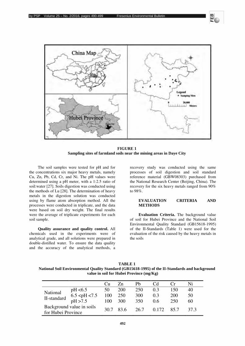
by PSP Volume 25 – No. 2/2016, pages 490-499 Fresenius Environmental Bulletin
492
FIGURE 1
Sampling sites of farmland soils near the mining areas in Daye City
The soil samples were tested for pH and for
the concentrations six major heavy metals, namely
Cu, Zn, Pb, Cd, Cr, and Ni. The pH values were
determined using a pH meter, with a 1:2.5 ratio of
soil:water [27]. Soils digestion was conducted using
the methods of Lu [28]. The determination of heavy
metals in the digestion solution was conducted
using by flame atom absorption method. All the
processes were conducted in triplicate, and the data
were based on soil dry weight. The final results
were the average of triplicate experiments for each
soil sample.
Quality assurance and quality control. All
chemicals used in the experiments were of
analytical grade, and all solutions were prepared in
double-distilled water. To ensure the data quality
and the accuracy of the analytical methods, a
recovery study was conducted using the same
processes of soil digestion and soil standard
reference material (GBW08303) purchased from
the National Research Center (Beijing, China). The
recovery for the six heavy metals ranged from 90%
to 98%.
EVALUATION CRITERIA AND
METHODS
Evaluation Criteria. The background value
of soil for Hubei Province and the National Soil
Environmental Quality Standard (GB15618-1995)
of the II-Standards (Table 1) were used for the
evaluation of the risk caused by the heavy metals in
the soils
TABLE 1
National Soil Environmental Quality Standard (GB15618-1995) of the II-Standards and background
value in soil for Hubei Province (mg/Kg)
Cu Zn Pb Cd Cr Ni
National
II-standard
pH <6.5 50 200 250 0.3 150 40
6.5 <pH <7.5 100 250 300 0.3 200 50
pH >7.5 100 300 350 0.6 250 60
Background value in soils
for Hubei Province 30.7 83.6 26.7 0.172 85.7 37.3
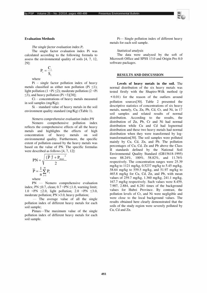
by PSP Volume 25 – No. 2/2016, pages 490-499 Fresenius Environmental Bulletin
493
Evaluation Methods
The single factor evaluation index Pi
The single factor evaluation index Pi was
calculated according to the following formula to
assess the environmental quality of soils [4, 7, 12,
29]:
i
ii
S
CP
where
Pi – single factor pollution index of heavy
metals classified as either non pollution (Pi ≤1); light pollution (1 <Pi ≤2); moderate pollution (2 <Pi ≤3), and heavy pollution (Pi >3)[30];
Ci – concentrations of heavy metals measured
in soil samples (mg/Kg);
Si – standard value of heavy metals in the soil
environment quality standard (mg/Kg) (Table 1).
Nemero comprehensive evaluation index PN
Nemero comprehensive pollution index
reflects the comprehensive effects of all the heavy
metals and highlights the effects of high
concentration of heavy metals on soil
environmental quality. Furthermore, the specific
extent of pollution caused by the heavy metals was
based on the value of PN. The specific formulas
were described as follows [4, 7, 12]:
2
PPPN
2
imax
2
i
m
1i
Pn
1P
where
PN — Nemero comprehensive evaluation
index; PN ≤0.7, clean; 0.7 <PN ≤1.0, warning limit; 1.0 <PN ≤2.0, light pollution; 2.0 <PN ≤3.0,
moderate pollution; PN >3.0, heavy pollution;
— The average value of all the single
pollution index of different heavy metals for each
soil sample;
Pimax—The maximum value of the single
pollution index of different heavy metals for each
soil sample.
Pi— Single pollution index of different heavy
metals for each soil sample.
Statistical analysis
The data were analyzed by the soft of
Microsoft Office and SPSS 13.0 and Origin Pro 8.0
software packages.
RESULTS AND DISCUSSION
Levels of heavy metals in the soil. The
normal distribution of the six heavy metals was
tested firstly with the Shapiro-Wilk method (p
<0.01) for the reason of the outliers around
pollution sources[30]. Table 2 presented the
descriptive statistics of concentrations of six heavy
metals, namely, Cu, Zn, Pb, Cd, Cr, and Ni, in 17
soil samples and related results of normal
distribution. According to the results, the
distribution of Zn, Pb, Cr and Ni had normal
distribution while Cu and Cd had lognormal
distribution and these two heavy metals had normal
distribution when they were transformed by log-
transformation[30]. The soil samples were polluted
mainly by Cu, Cd, Zn, and Pb. The pollution
percentages of Cu, Cd, Zn and Pb above the Class
II standards defined by the National Soil
Environmental Quality Standard (GB15618-1995)
were 88.24%, 100%, 58.82%, and 11.76%
respectively. The concentration ranges were 25.39
mg/kg to 1121 mg/kg, 0.5237 mg/kg to 5.45 mg/kg,
58.64 mg/kg to 559.5 mg/kg, and 51.97 mg/kg to
465.8 mg/kg for Cu, Cd, Zn, and Pb, with mean
values of 259.7 mg/kg, 1.360 mg/kg, 241.1 mg/kg,
167.7 mg/kg respectively. Such values were 8.459,
7.907, 2.884, and 6.281 times of the background
values for Hubei Province. By contrast, the
pollution levels of Cr, and Ni were negligible and
were close to the local background values. The
results obtained here clearly demonstrated that the
soils of the study region were severely polluted by
Cu, Cd and Zn.
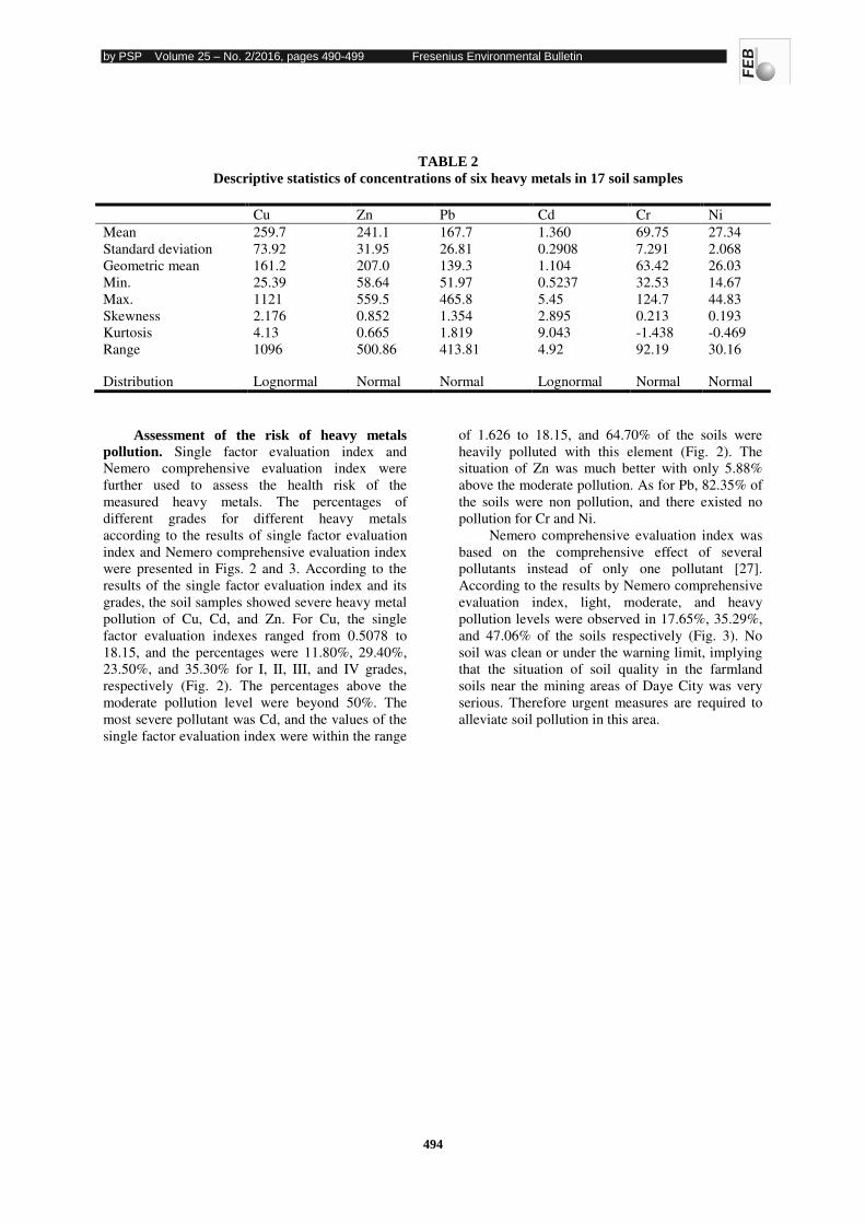
by PSP Volume 25 – No. 2/2016, pages 490-499 Fresenius Environmental Bulletin
494
TABLE 2
Descriptive statistics of concentrations of six heavy metals in 17 soil samples
Cu Zn Pb Cd Cr Ni
Mean 259.7 241.1 167.7 1.360 69.75 27.34
Standard deviation 73.92 31.95 26.81 0.2908 7.291 2.068
Geometric mean 161.2 207.0 139.3 1.104 63.42 26.03
Min. 25.39 58.64 51.97 0.5237 32.53 14.67
Max. 1121 559.5 465.8 5.45 124.7 44.83
Skewness 2.176 0.852 1.354 2.895 0.213 0.193
Kurtosis 4.13 0.665 1.819 9.043 -1.438 -0.469
Range 1096 500.86 413.81 4.92 92.19 30.16
Distribution Lognormal Normal Normal Lognormal Normal Normal
Assessment of the risk of heavy metals
pollution. Single factor evaluation index and
Nemero comprehensive evaluation index were
further used to assess the health risk of the
measured heavy metals. The percentages of
different grades for different heavy metals
according to the results of single factor evaluation
index and Nemero comprehensive evaluation index
were presented in Figs. 2 and 3. According to the
results of the single factor evaluation index and its
grades, the soil samples showed severe heavy metal
pollution of Cu, Cd, and Zn. For Cu, the single
factor evaluation indexes ranged from 0.5078 to
18.15, and the percentages were 11.80%, 29.40%,
23.50%, and 35.30% for I, II, III, and IV grades,
respectively (Fig. 2). The percentages above the
moderate pollution level were beyond 50%. The
most severe pollutant was Cd, and the values of the
single factor evaluation index were within the range
of 1.626 to 18.15, and 64.70% of the soils were
heavily polluted with this element (Fig. 2). The
situation of Zn was much better with only 5.88%
above the moderate pollution. As for Pb, 82.35% of
the soils were non pollution, and there existed no
pollution for Cr and Ni.
Nemero comprehensive evaluation index was
based on the comprehensive effect of several
pollutants instead of only one pollutant [27].
According to the results by Nemero comprehensive
evaluation index, light, moderate, and heavy
pollution levels were observed in 17.65%, 35.29%,
and 47.06% of the soils respectively (Fig. 3). No
soil was clean or under the warning limit, implying
that the situation of soil quality in the farmland
soils near the mining areas of Daye City was very
serious. Therefore urgent measures are required to
alleviate soil pollution in this area.
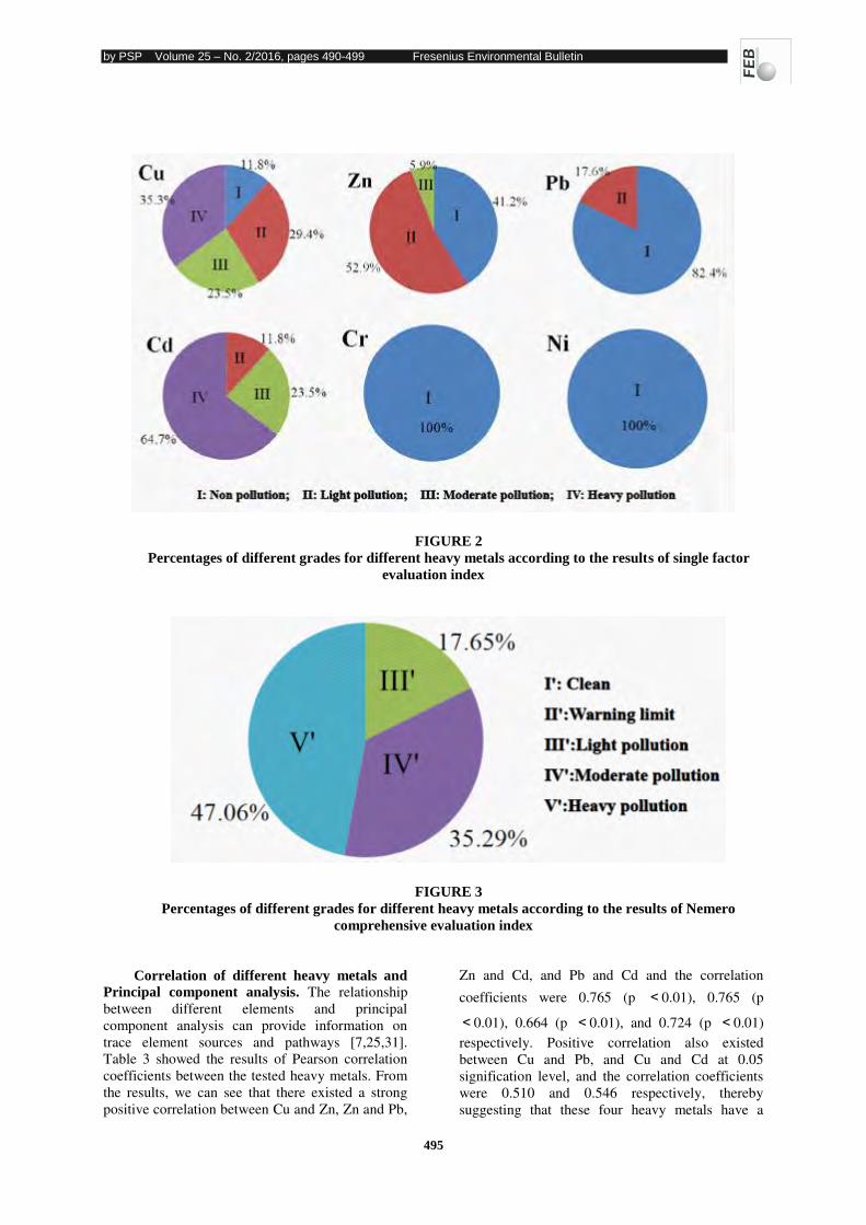
by PSP Volume 25 – No. 2/2016, pages 490-499 Fresenius Environmental Bulletin
495
FIGURE 2
Percentages of different grades for different heavy metals according to the results of single factor
evaluation index
FIGURE 3
Percentages of different grades for different heavy metals according to the results of Nemero
comprehensive evaluation index
Correlation of different heavy metals and
Principal component analysis. The relationship
between different elements and principal
component analysis can provide information on
trace element sources and pathways [7,25,31].
Table 3 showed the results of Pearson correlation
coefficients between the tested heavy metals. From
the results, we can see that there existed a strong
positive correlation between Cu and Zn, Zn and Pb,
Zn and Cd, and Pb and Cd and the correlation
coefficients were 0.765 (p <0.01), 0.765 (p
<0.01), 0.664 (p <0.01), and 0.724 (p <0.01)
respectively. Positive correlation also existed
between Cu and Pb, and Cu and Cd at 0.05
signification level, and the correlation coefficients
were 0.510 and 0.546 respectively, thereby
suggesting that these four heavy metals have a
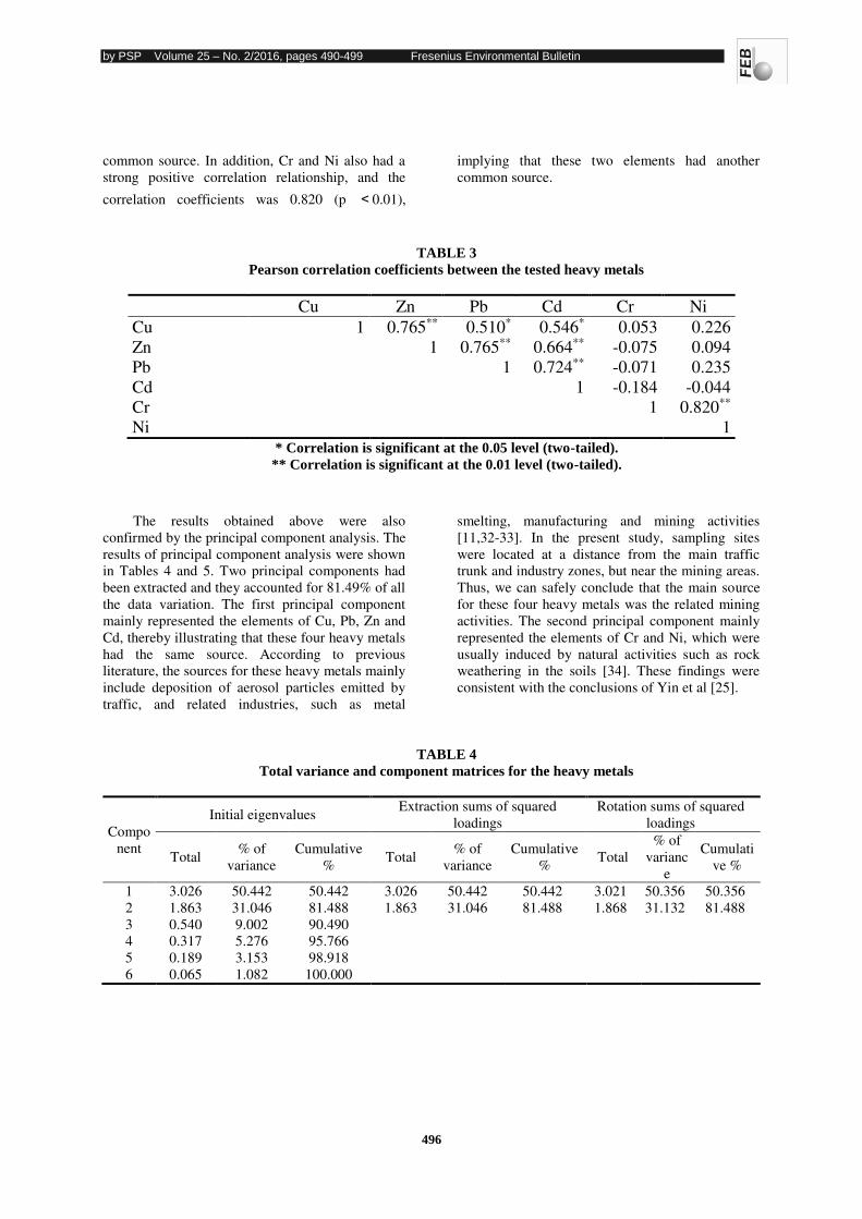
by PSP Volume 25 – No. 2/2016, pages 490-499 Fresenius Environmental Bulletin
496
common source. In addition, Cr and Ni also had a
strong positive correlation relationship, and the
correlation coefficients was 0.820 (p <0.01),
implying that these two elements had another
common source.
TABLE 3
Pearson correlation coefficients between the tested heavy metals
Cu Zn Pb Cd Cr Ni
Cu 1 0.765** 0.510* 0.546* 0.053 0.226
Zn 1 0.765** 0.664** -0.075 0.094
Pb 1 0.724** -0.071 0.235
Cd 1 -0.184 -0.044
Cr 1 0.820**
Ni 1
* Correlation is significant at the 0.05 level (two-tailed).
** Correlation is significant at the 0.01 level (two-tailed).
The results obtained above were also
confirmed by the principal component analysis. The
results of principal component analysis were shown
in Tables 4 and 5. Two principal components had
been extracted and they accounted for 81.49% of all
the data variation. The first principal component
mainly represented the elements of Cu, Pb, Zn and
Cd, thereby illustrating that these four heavy metals
had the same source. According to previous
literature, the sources for these heavy metals mainly
include deposition of aerosol particles emitted by
traffic, and related industries, such as metal
smelting, manufacturing and mining activities
[11,32-33]. In the present study, sampling sites
were located at a distance from the main traffic
trunk and industry zones, but near the mining areas.
Thus, we can safely conclude that the main source
for these four heavy metals was the related mining
activities. The second principal component mainly
represented the elements of Cr and Ni, which were
usually induced by natural activities such as rock
weathering in the soils [34]. These findings were
consistent with the conclusions of Yin et al [25].
TABLE 4
Total variance and component matrices for the heavy metals
Compo
nent
Initial eigenvalues Extraction sums of squared
loadings
Rotation sums of squared
loadings
Total % of
variance
Cumulative
% Total
% of
variance
Cumulative
% Total
% of
varianc
e
Cumulati
ve %
1 3.026 50.442 50.442 3.026 50.442 50.442 3.021 50.356 50.356
2 1.863 31.046 81.488 1.863 31.046 81.488 1.868 31.132 81.488
3 0.540 9.002 90.490
4 0.317 5.276 95.766
5 0.189 3.153 98.918
6 0.065 1.082 100.000
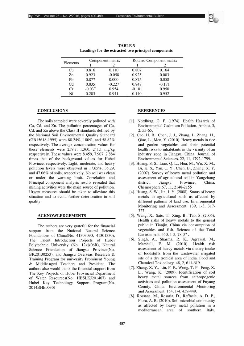
by PSP Volume 25 – No. 2/2016, pages 490-499 Fresenius Environmental Bulletin
497
TABLE 5
Loadings for the extracted two principal components
Elements Component matrix Rotated Component matrix
1 2 1 2
Cu 0.816 0.110 0.807 0.164
Zn 0.923 -0.058 0.925 0.003
Pb 0.877 0.000 0.875 0.058
Cd 0.835 -0.227 0.848 -0.171
Cr -0.037 0.954 -0.101 0.950
Ni 0.203 0.941 0.140 0.952
CONCLUSIONS
The soils sampled were severely polluted with
Cu, Cd, and Zn. The pollution percentages of Cu,
Cd, and Zn above the Class II standards defined by
the National Soil Environmental Quality Standard
(GB15618-1995) were 88.24%, 100%, and 58.82%
respectively. The average concentration values for
these elements were 259.7, 1.360, 241.1 mg/kg
respectively. These values were 8.459, 7.907, 2.884
times that of the background values for Hubei
Province, respectively. Light, moderate, and heavy
pollution levels were observed in 17.65%, 35.29,
and 47.06% of soils, respectively. No soil was clean
or under the warning limit. Correlation and
Principal component analysis results revealed that
mining activities were the main source of pollution.
Urgent measures should be taken to alleviate this
situation and to avoid further deterioration in soil
quality.
ACKNOWLEDGEMENTS
The authors are very grateful for the financial
support from the National Natural Science
Foundations of China(No. 41303090; 41301330),
The Talent Introduction Projects of Hubei
Polytechnic University (No. 12xjz06R), Natural
Science Foundation of Jiangsu Province(No.
BK20130253), and Jiangsu Overseas Research &
Training Program for university Prominent Young
& Middle-aged Teachers and President. The
authors also would thank the financial support from
The Key Projects of Hubei Provincial Department
of Water Resources(No. HBSLKJ201407) and
Hubei Key Technology Support Program(No.
2014BHE0030)
REFERENCES
[1]. Nordberg, G. F. (1974). Health Hazards of
Environmental Cadmium Pollution. Ambio. 3,
2, 55-65.
[2]. Cao, H. B., Chen, J. J., Zhang, J., Zhang, H.,
Qiao, L., Men, Y. (2010). Heavy metals in rice
and garden vegetables and their potential
health risks to inhabitants in the vicinity of an
industry zone in Jiangsu, China. Journal of
Environmental Sciences. 22, 11, 1792-1799.
[3]. Huang, S. S., Liao, Q. L., Hua, M., Wu, X. M.,
Bi, K. S., Yan, C. Y., Chen, B., Zhang, X. Y.
(2007). Survey of heavy metal pollution and
assessment of agricultural soil in Yangzhong
district, Jiangsu Province, China.
Chemosphere.67, 11, 2148-2155
[4]. Huang, S. W., Jin, J. Y. (2008). Status of heavy
metals in agricultural soils as affected by
different patterns of land use. Environmental
Monitoring and Assessment. 139, 1-3, 317-
327.
[5]. Wang, X., Sato, T., Xing, B., Tao, S. (2005).
Health risks of heavy metals to the general
public in Tianjin, China via consumption of
vegetables and fish. Science of the Total
Environment. 350, 1-3, 28-37 .
[6]. Singh, A., Sharma, R. K., Agrawal, M.,
Marshall, F. M. (2010). Health risk
assessment of heavy metals via dietary intake
of foodstuffs from the wastewater irrigated
site of a dry tropical area of India. Food and
Chemical Toxicology. 48, 2, 611-619.
[7]. Zhang, X. Y., Lin, F. F., Wong, T. F., Feng, X.
L., Wang, K. (2009). Identification of soil
heavy metal sources from anthropogenic
activities and pollution assessment of Fuyang
County, China. Environmental Monitoring
and Assessment. 154, 1-4, 439-449.
[8]. Rossana, M., Rosaria, D., Raffaele, A. D. P.,
Flora, A. R. (2010). Soil microbial community
as affected by heavy metal pollution in a
mediterranean area of southern Italy.
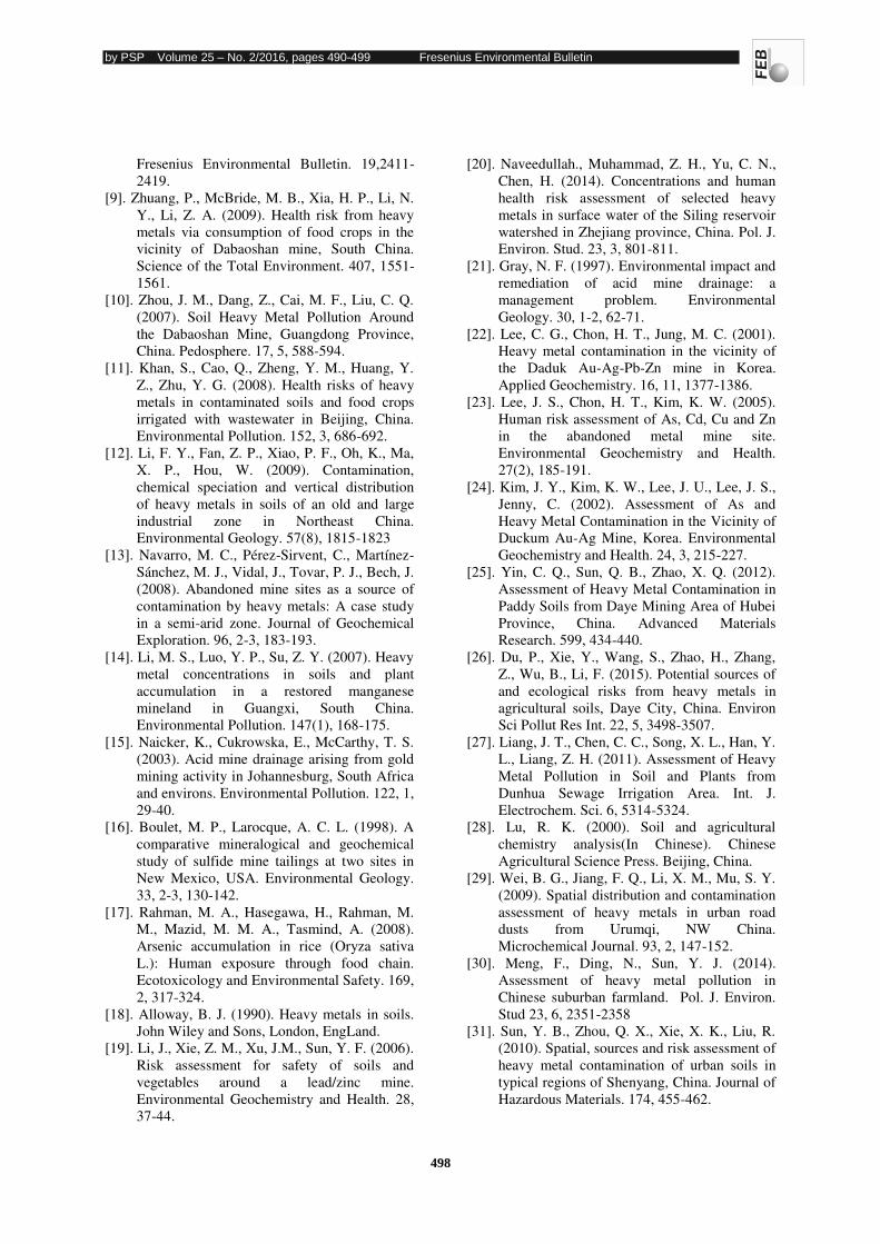
by PSP Volume 25 – No. 2/2016, pages 490-499 Fresenius Environmental Bulletin
498
Fresenius Environmental Bulletin. 19,2411-
2419.
[9]. Zhuang, P., McBride, M. B., Xia, H. P., Li, N.
Y., Li, Z. A. (2009). Health risk from heavy
metals via consumption of food crops in the
vicinity of Dabaoshan mine, South China.
Science of the Total Environment. 407, 1551-
1561.
[10]. Zhou, J. M., Dang, Z., Cai, M. F., Liu, C. Q.
(2007). Soil Heavy Metal Pollution Around
the Dabaoshan Mine, Guangdong Province,
China. Pedosphere. 17, 5, 588-594.
[11]. Khan, S., Cao, Q., Zheng, Y. M., Huang, Y.
Z., Zhu, Y. G. (2008). Health risks of heavy
metals in contaminated soils and food crops
irrigated with wastewater in Beijing, China.
Environmental Pollution. 152, 3, 686-692.
[12]. Li, F. Y., Fan, Z. P., Xiao, P. F., Oh, K., Ma,
X. P., Hou, W. (2009). Contamination,
chemical speciation and vertical distribution
of heavy metals in soils of an old and large
industrial zone in Northeast China.
Environmental Geology. 57(8), 1815-1823
[13]. Navarro, M. C., Pérez-Sirvent, C., Martínez-
Sánchez, M. J., Vidal, J., Tovar, P. J., Bech, J.
(2008). Abandoned mine sites as a source of
contamination by heavy metals: A case study
in a semi-arid zone. Journal of Geochemical
Exploration. 96, 2-3, 183-193.
[14]. Li, M. S., Luo, Y. P., Su, Z. Y. (2007). Heavy
metal concentrations in soils and plant
accumulation in a restored manganese
mineland in Guangxi, South China.
Environmental Pollution. 147(1), 168-175.
[15]. Naicker, K., Cukrowska, E., McCarthy, T. S.
(2003). Acid mine drainage arising from gold
mining activity in Johannesburg, South Africa
and environs. Environmental Pollution. 122, 1,
29-40.
[16]. Boulet, M. P., Larocque, A. C. L. (1998). A
comparative mineralogical and geochemical
study of sulfide mine tailings at two sites in
New Mexico, USA. Environmental Geology.
33, 2-3, 130-142.
[17]. Rahman, M. A., Hasegawa, H., Rahman, M.
M., Mazid, M. M. A., Tasmind, A. (2008).
Arsenic accumulation in rice (Oryza sativa
L.): Human exposure through food chain.
Ecotoxicology and Environmental Safety. 169,
2, 317-324.
[18]. Alloway, B. J. (1990). Heavy metals in soils.
John Wiley and Sons, London, EngLand.
[19]. Li, J., Xie, Z. M., Xu, J.M., Sun, Y. F. (2006).
Risk assessment for safety of soils and
vegetables around a lead/zinc mine.
Environmental Geochemistry and Health. 28,
37-44.
[20]. Naveedullah., Muhammad, Z. H., Yu, C. N.,
Chen, H. (2014). Concentrations and human
health risk assessment of selected heavy
metals in surface water of the Siling reservoir
watershed in Zhejiang province, China. Pol. J.
Environ. Stud. 23, 3, 801-811.
[21]. Gray, N. F. (1997). Environmental impact and
remediation of acid mine drainage: a
management problem. Environmental
Geology. 30, 1-2, 62-71.
[22]. Lee, C. G., Chon, H. T., Jung, M. C. (2001).
Heavy metal contamination in the vicinity of
the Daduk Au-Ag-Pb-Zn mine in Korea.
Applied Geochemistry. 16, 11, 1377-1386.
[23]. Lee, J. S., Chon, H. T., Kim, K. W. (2005).
Human risk assessment of As, Cd, Cu and Zn
in the abandoned metal mine site.
Environmental Geochemistry and Health.
27(2), 185-191.
[24]. Kim, J. Y., Kim, K. W., Lee, J. U., Lee, J. S.,
Jenny, C. (2002). Assessment of As and
Heavy Metal Contamination in the Vicinity of
Duckum Au-Ag Mine, Korea. Environmental
Geochemistry and Health. 24, 3, 215-227.
[25]. Yin, C. Q., Sun, Q. B., Zhao, X. Q. (2012).
Assessment of Heavy Metal Contamination in
Paddy Soils from Daye Mining Area of Hubei
Province, China. Advanced Materials
Research. 599, 434-440.
[26]. Du, P., Xie, Y., Wang, S., Zhao, H., Zhang,
Z., Wu, B., Li, F. (2015). Potential sources of
and ecological risks from heavy metals in
agricultural soils, Daye City, China. Environ
Sci Pollut Res Int. 22, 5, 3498-3507.
[27]. Liang, J. T., Chen, C. C., Song, X. L., Han, Y.
L., Liang, Z. H. (2011). Assessment of Heavy
Metal Pollution in Soil and Plants from
Dunhua Sewage Irrigation Area. Int. J.
Electrochem. Sci. 6, 5314-5324.
[28]. Lu, R. K. (2000). Soil and agricultural
chemistry analysis(In Chinese). Chinese
Agricultural Science Press. Beijing, China.
[29]. Wei, B. G., Jiang, F. Q., Li, X. M., Mu, S. Y.
(2009). Spatial distribution and contamination
assessment of heavy metals in urban road
dusts from Urumqi, NW China.
Microchemical Journal. 93, 2, 147-152.
[30]. Meng, F., Ding, N., Sun, Y. J. (2014).
Assessment of heavy metal pollution in
Chinese suburban farmland. Pol. J. Environ.
Stud 23, 6, 2351-2358
[31]. Sun, Y. B., Zhou, Q. X., Xie, X. K., Liu, R.
(2010). Spatial, sources and risk assessment of
heavy metal contamination of urban soils in
typical regions of Shenyang, China. Journal of
Hazardous Materials. 174, 455-462.
by PSP Volume 25 – No. 2/2016, pages 490-499 Fresenius Environmental Bulletin
499
[32]. Gray, C. W., McLaren, R. G., Roberts, A. H.
C. (2003). Atmospheric accessions of heavy
metals to some New Zealand pastoral soils.
Science of the Total Environment. 305, 105-
115.
[33]. Habes, G., Nigem, Y. (2006). Assessing Mn,
Fe, Cu, Zn, and Cd pollution in bottom
sediments of Wadi Al-Arab Dam, Jordan.
Chemosphere. 65, 11, 2114-2121.
[34]. Chen, T. B., Zheng, Y. M., Lei, M., Huang, Z.
C., Wu, H. T., Chen, H., Fan, K. K., Yu, K.,
Wu, X., Tian, Q. Z. (2005). Assessment of
heavy metal pollution in surface soils of urban
parks in Beijing, China. Chemosphere. 60, 4,
542-551.
Received: 25.06.2015 Accepted: 16.12.2015
CORRESPONDING AUTHOR
Yongkui Wang College of Environmental Science and Engineering
Hubei Polytechnic University
Huangshi 435003, Hubei – P.R. CHINA
email: [email protected]
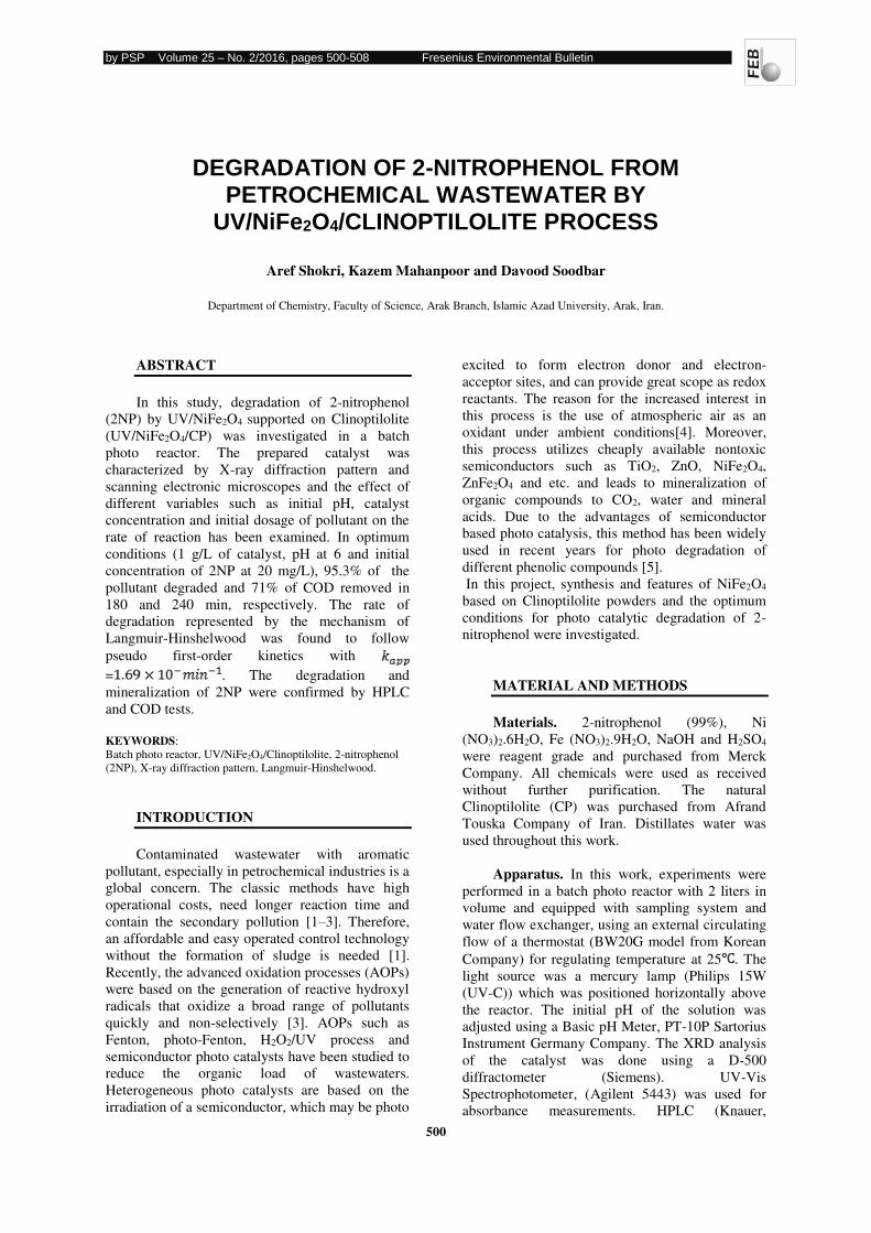
by PSP Volume 25 – No. 2/2016, pages 500-508 Fresenius Environmental Bulletin
500
DEGRADATION OF 2-NITROPHENOL FROM PETROCHEMICAL WASTEWATER BY
UV/NiFe2O4/CLINOPTILOLITE PROCESS
Aref Shokri, Kazem Mahanpoor and Davood Soodbar
Department of Chemistry, Faculty of Science, Arak Branch, Islamic Azad University, Arak, Iran.
ABSTRACT
In this study, degradation of 2-nitrophenol
(2NP) by UV/NiFe2O4 supported on Clinoptilolite
(UV/NiFe2O4/CP) was investigated in a batch
photo reactor. The prepared catalyst was
characterized by X-ray diffraction pattern and
scanning electronic microscopes and the effect of
different variables such as initial pH, catalyst
concentration and initial dosage of pollutant on the
rate of reaction has been examined. In optimum
conditions (1 g/L of catalyst, pH at 6 and initial
concentration of 2NP at 20 mg/L), 95.3% of the
pollutant degraded and 71% of COD removed in
180 and 240 min, respectively. The rate of
degradation represented by the mechanism of
Langmuir-Hinshelwood was found to follow
pseudo first-order kinetics with
= . The degradation and
mineralization of 2NP were confirmed by HPLC
and COD tests.
KEYWORDS:
Batch photo reactor, UV/NiFe2O4/Clinoptilolite, 2-nitrophenol
(2NP), X-ray diffraction pattern, Langmuir-Hinshelwood.
INTRODUCTION
Contaminated wastewater with aromatic
pollutant, especially in petrochemical industries is a
global concern. The classic methods have high
operational costs, need longer reaction time and
contain the secondary pollution [1–3]. Therefore,
an affordable and easy operated control technology
without the formation of sludge is needed [1].
Recently, the advanced oxidation processes (AOPs)
were based on the generation of reactive hydroxyl
radicals that oxidize a broad range of pollutants
quickly and non-selectively [3]. AOPs such as
Fenton, photo-Fenton, H2O2/UV process and
semiconductor photo catalysts have been studied to
reduce the organic load of wastewaters.
Heterogeneous photo catalysts are based on the
irradiation of a semiconductor, which may be photo
excited to form electron donor and electron-
acceptor sites, and can provide great scope as redox
reactants. The reason for the increased interest in
this process is the use of atmospheric air as an
oxidant under ambient conditions[4]. Moreover,
this process utilizes cheaply available nontoxic
semiconductors such as TiO2, ZnO, NiFe2O4,
ZnFe2O4 and etc. and leads to mineralization of
organic compounds to CO2, water and mineral
acids. Due to the advantages of semiconductor
based photo catalysis, this method has been widely
used in recent years for photo degradation of
different phenolic compounds [5].
In this project, synthesis and features of NiFe2O4
based on Clinoptilolite powders and the optimum
conditions for photo catalytic degradation of 2-
nitrophenol were investigated.
MATERIAL AND METHODS
Materials. 2-nitrophenol (99%), Ni
(NO3)2.6H2O, Fe (NO3)2.9H2O, NaOH and H2SO4
were reagent grade and purchased from Merck
Company. All chemicals were used as received
without further purification. The natural
Clinoptilolite (CP) was purchased from Afrand
Touska Company of Iran. Distillates water was
used throughout this work.
Apparatus. In this work, experiments were
performed in a batch photo reactor with 2 liters in
volume and equipped with sampling system and
water flow exchanger, using an external circulating
flow of a thermostat (BW20G model from Korean
Company) for regulating temperature at 25 . The
light source was a mercury lamp (Philips 15W
(UV-C)) which was positioned horizontally above
the reactor. The initial pH of the solution was
adjusted using a Basic pH Meter, PT-10P Sartorius
Instrument Germany Company. The XRD analysis
of the catalyst was done using a D-500
diffractometer (Siemens). UV-Vis
Spectrophotometer, (Agilent 5443) was used for
absorbance measurements. HPLC (Knauer,
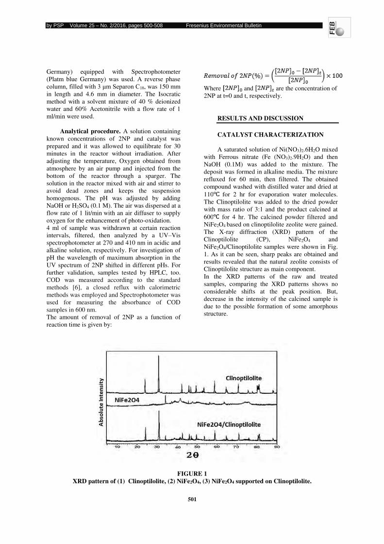
by PSP Volume 25 – No. 2/2016, pages 500-508 Fresenius Environmental Bulletin
501
Germany) equipped with Spectrophotometer
(Platm blue Germany) was used. A reverse phase
column, filled with 3 μm Separon C18, was 150 mm
in length and 4.6 mm in diameter. The Isocratic
method with a solvent mixture of 40 % deionized
water and 60% Acetonitrile with a flow rate of 1
ml/min were used.
Analytical procedure. A solution containing
known concentrations of 2NP and catalyst was
prepared and it was allowed to equilibrate for 30
minutes in the reactor without irradiation. After
adjusting the temperature, Oxygen obtained from
atmosphere by an air pump and injected from the
bottom of the reactor through a sparger. The
solution in the reactor mixed with air and stirrer to
avoid dead zones and keeps the suspension
homogenous. The pH was adjusted by adding
NaOH or H2SO4 (0.1 M). The air was dispersed at a
flow rate of 1 lit/min with an air diffuser to supply
oxygen for the enhancement of photo-oxidation.
4 ml of sample was withdrawn at certain reaction
intervals, filtered, then analyzed by a UV–Vis
spectrophotometer at 270 and 410 nm in acidic and
alkaline solution, respectively. For investigation of
pH the wavelength of maximum absorption in the
UV spectrum of 2NP shifted in different pHs. For
further validation, samples tested by HPLC, too.
COD was measured according to the standard
methods [6], a closed reflux with calorimetric
methods was employed and Spectrophotometer was
used for measuring the absorbance of COD
samples in 600 nm.
The amount of removal of 2NP as a function of
reaction time is given by:
Where and are the concentration of
2NP at t=0 and t, respectively.
RESULTS AND DISCUSSION
CATALYST CHARACTERIZATION
A saturated solution of Ni(NO3)2.6H2O mixed
with Ferrous nitrate (Fe (NO3)2.9H2O) and then
NaOH (0.1M) was added to the mixture. The
deposit was formed in alkaline media. The mixture
refluxed for 60 min, then filtered. The obtained
compound washed with distilled water and dried at
110 for 2 hr for evaporation water molecules.
The Clinoptilolite was added to the dried powder
with mass ratio of 3:1 and the product calcined at
600 for 4 hr. The calcined powder filtered and
NiFe2O4 based on clinoptilolite zeolite were gained.
The X-ray diffraction (XRD) pattern of the
Clinoptilolite (CP), NiFe2O4 and
NiFe2O4/Clinoptilolite samples were shown in Fig.
1. As it can be seen, sharp peaks are obtained and
results revealed that the natural zeolite consists of
Clinoptilolite structure as main component.
In the XRD patterns of the raw and treated
samples, comparing the XRD patterns shows no
considerable shifts at the peak position. But,
decrease in the intensity of the calcined sample is
due to the possible formation of some amorphous
structure.
FIGURE 1
XRD pattern of (1) Clinoptilolite, (2) NiFe2O4, (3) NiFe2O4 supported on Clinoptilolite.
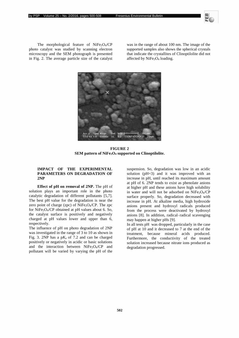
by PSP Volume 25 – No. 2/2016, pages 500-508 Fresenius Environmental Bulletin
502
The morphological feature of NiFe2O4/CP
photo catalyst was studied by scanning electron
microscopy and the SEM photograph is presented
in Fig. 2. The average particle size of the catalyst
was in the range of about 100 nm. The image of the
supported samples also shows the spherical crystals
that indicate the crystallites of Clinoptilolite did not
affected by NiFe2O4 loading.
FIGURE 2
SEM pattern of NiFe2O4 supported on Clinoptilolite.
IMPACT OF THE EXPERIMENTAL
PARAMETERS ON DEGRADATION OF
2NP
Effect of pH on removal of 2NP. The pH of
solution plays an important role in the photo
catalytic degradation of different pollutants [5,7].
The best pH value for the degradation is near the
zero point of charge (zpc) of NiFe2O4/CP. The zpc
for NiFe2O4/CP obtained at pH values about 6. So,
the catalyst surface is positively and negatively
charged at pH values lower and upper than 6,
respectively.
The influence of pH on photo degradation of 2NP
was investigated in the range of 3 to 10 as shown in
Fig. 3. 2NP has a pKa of 7.2 and can be charged
positively or negatively in acidic or basic solutions
and the interaction between NiFe2O4/CP and
pollutant will be varied by varying the pH of the
suspension. So, degradation was low in an acidic
solution (pH=3) and it was improved with an
increase in pH, until reached its maximum amount
at pH of 6. 2NP tends to exist as phenolate anions
at higher pH and these anions have high solubility
in water and will not be adsorbed on NiFe2O4/CP
surface properly. So, degradation decreased with
increase in pH. At alkaline media, high hydroxide
anions present and hydroxyl radicals produced
from the process were deactivated by hydroxyl
anions [8]. In addition, radical–radical scavenging
may happen at higher pHs [9].
In all tests pH was dropped, particularly in the case
of pH at 10 and it decreased to 7 at the end of the
treatment, because mineral acids produced.
Furthermore, the conductivity of the treated
solution increased because nitrate ions produced as
degradation progressed.
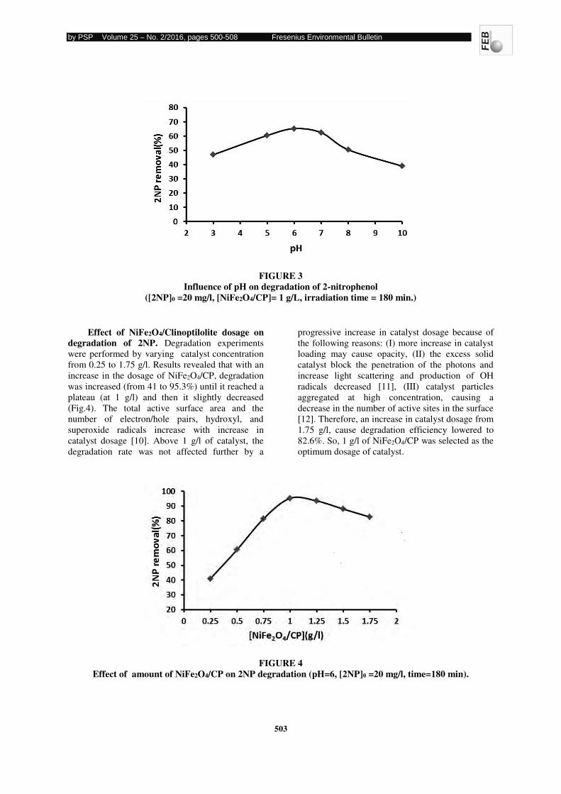
by PSP Volume 25 – No. 2/2016, pages 500-508 Fresenius Environmental Bulletin
503
FIGURE 3
Influence of pH on degradation of 2-nitrophenol
([2NP]0 =20 mg/l, [NiFe2O4/CP]= 1 g/L, irradiation time = 180 min.)
Effect of NiFe2O4/Clinoptilolite dosage on
degradation of 2NP. Degradation experiments
were performed by varying catalyst concentration
from 0.25 to 1.75 g/l. Results revealed that with an
increase in the dosage of NiFe2O4/CP, degradation
was increased (from 41 to 95.3%) until it reached a
plateau (at 1 g/l) and then it slightly decreased
(Fig.4). The total active surface area and the
number of electron/hole pairs, hydroxyl, and
superoxide radicals increase with increase in
catalyst dosage [10]. Above 1 g/l of catalyst, the
degradation rate was not affected further by a
progressive increase in catalyst dosage because of
the following reasons: (I) more increase in catalyst
loading may cause opacity, (II) the excess solid
catalyst block the penetration of the photons and
increase light scattering and production of OH
radicals decreased [11], (III) catalyst particles
aggregated at high concentration, causing a
decrease in the number of active sites in the surface
[12]. Therefore, an increase in catalyst dosage from
1.75 g/l, cause degradation efficiency lowered to
82.6%. So, 1 g/l of NiFe2O4/CP was selected as the
optimum dosage of catalyst.
FIGURE 4
Effect of amount of NiFe2O4/CP on 2NP degradation (pH=6, [2NP]0 =20 mg/l, time=180 min).
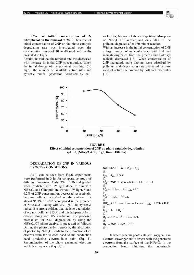
by PSP Volume 25 – No. 2/2016, pages 500-508 Fresenius Environmental Bulletin
504
Effect of initial concentration of 2-
nitrophenol on the removal of 2NP. The effect of
initial concentration of 2NP on the photo catalytic
degradation rate was investigated over the
concentration range of 10 to 40 mg/l and results
presented in Fig.5.
Results showed that the removal rate was decreased
with increase in initial 2NP concentration. When
the initial dosage of the pollutant was high (40
mg/l), the number of available active sites and
hydroxyl radical generation decreased by 2NP
molecules, because of their competitive adsorption
on NiFe2O4/CP surface and only 58% of the
pollutant degraded after 180 min of reaction.
With an increase in the initial concentration of 2NP
a large number of molecules react with hydroxyl
radicals originated from the process and hydroxyl
radicals decreased [13]. When concentration of
2NP increased, more photons were adsorbed by
pollutant and degradation rate decreased because
most of active site covered by pollutant molecules
[14].
FIGURE 5
Effect of initial concentration of 2NP on photo catalytic degradation
(pH=6, [NiFe2O4/CP] =1g/l, time =180min).
DEGRADATION OF 2NP IN VARIOUS
PROCESS CONDITIONS
As it can be seen from Fig.6, experiments
were performed in 3 hr for comparative study of
different processes. Only 2% of 2NP degraded
when irradiated with UV light alone. In runs with
NiFe2O4 and Clinoptilolite without UV light, 5 and
6.2% of 2NP concentration decreased respectively,
because pollutant adsorbed on the surface. But
almost 95.3% of 2NP decomposed in the presence
of NiFe2O4/CP along with UV light. The hydroxyl
radical is a strong oxidant that leads to degradation
of organic pollutant [15,9] and this happens only in
catalyst along with UV irradiation. The proposed
mechanism for 2-NP degradation by using the
NiFe2O4/CP photo catalyst is suggested as follows:
During the photo catalytic process, the absorption
of photon by NiFe2O4 leads to the promotion of an
electron from the valence band to the conduction
band producing electron–hole pairs (Eq. 1).
Recombination of the photo generated electrons
and holes may occur (Eq. (2)).
NiFe2O4/CP + hv +
(1)
+ heat
(2)
+ 2NP intermediates CO2 + H2O
(3)
+ H2O (ads) + H+
(4)
+
(5)
+ 2NP (ads) intermediates + CO2 + H2O
(6)
+ O2
(7)
+ + O2 + H2O2
(8)
+ 2NP
(9)
In heterogeneous photo catalysis, oxygen is an
electron scavenger and it reacts with the generated
electrons from the surface of the NiFe2O4 in the
conduction band, inhibiting the undesirable
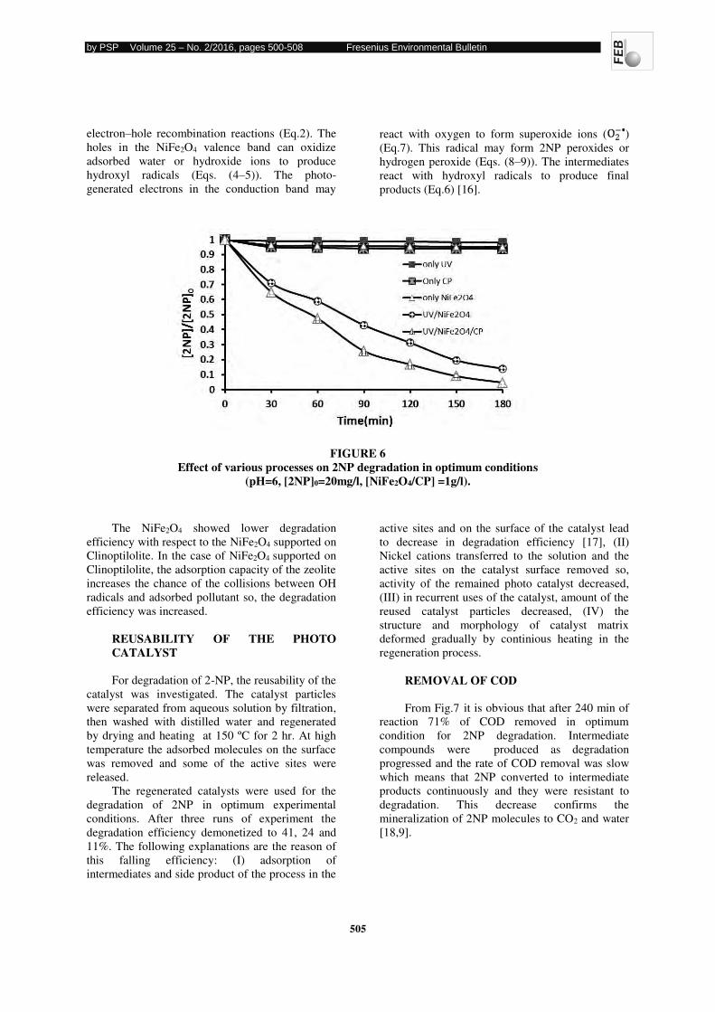
by PSP Volume 25 – No. 2/2016, pages 500-508 Fresenius Environmental Bulletin
505
electron–hole recombination reactions (Eq.2). The
holes in the NiFe2O4 valence band can oxidize
adsorbed water or hydroxide ions to produce
hydroxyl radicals (Eqs. (4–5)). The photo-
generated electrons in the conduction band may
react with oxygen to form superoxide ions ( )
(Eq.7). This radical may form 2NP peroxides or
hydrogen peroxide (Eqs. (8–9)). The intermediates
react with hydroxyl radicals to produce final
products (Eq.6) [16].
FIGURE 6
Effect of various processes on 2NP degradation in optimum conditions
(pH=6, [2NP]0=20mg/l, [NiFe2O4/CP] =1g/l).
The NiFe2O4 showed lower degradation
efficiency with respect to the NiFe2O4 supported on
Clinoptilolite. In the case of NiFe2O4 supported on
Clinoptilolite, the adsorption capacity of the zeolite
increases the chance of the collisions between OH
radicals and adsorbed pollutant so, the degradation
efficiency was increased.
REUSABILITY OF THE PHOTO
CATALYST
For degradation of 2-NP, the reusability of the
catalyst was investigated. The catalyst particles
were separated from aqueous solution by filtration,
then washed with distilled water and regenerated
by drying and heating at 150 ºC for 2 hr. At high
temperature the adsorbed molecules on the surface
was removed and some of the active sites were
released.
The regenerated catalysts were used for the
degradation of 2NP in optimum experimental
conditions. After three runs of experiment the
degradation efficiency demonetized to 41, 24 and
11%. The following explanations are the reason of
this falling efficiency: (I) adsorption of
intermediates and side product of the process in the
active sites and on the surface of the catalyst lead
to decrease in degradation efficiency [17], (II)
Nickel cations transferred to the solution and the
active sites on the catalyst surface removed so,
activity of the remained photo catalyst decreased,
(III) in recurrent uses of the catalyst, amount of the
reused catalyst particles decreased, (IV) the
structure and morphology of catalyst matrix
deformed gradually by continious heating in the
regeneration process.
REMOVAL OF COD
From Fig.7 it is obvious that after 240 min of
reaction 71% of COD removed in optimum
condition for 2NP degradation. Intermediate
compounds were produced as degradation
progressed and the rate of COD removal was slow
which means that 2NP converted to intermediate
products continuously and they were resistant to
degradation. This decrease confirms the
mineralization of 2NP molecules to CO2 and water
[18,9].
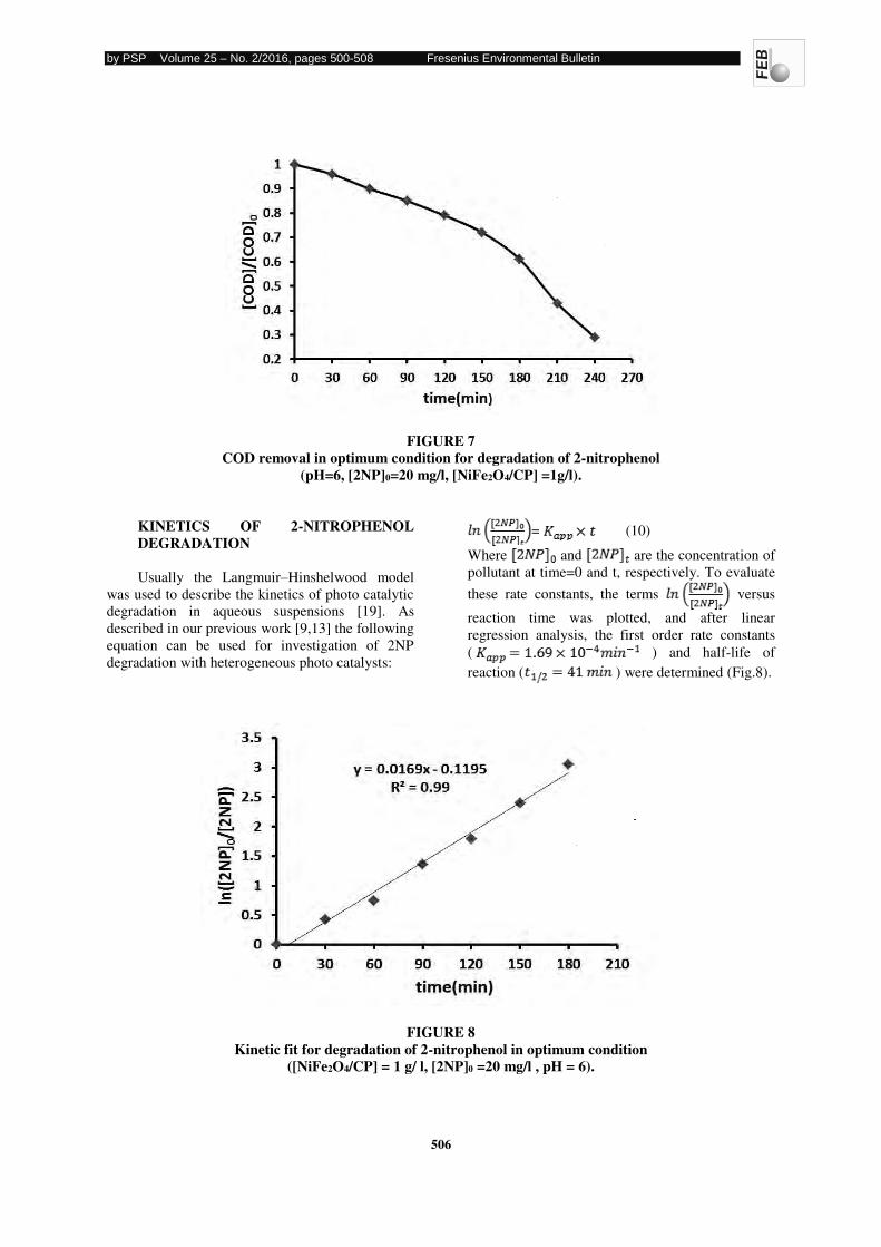
by PSP Volume 25 – No. 2/2016, pages 500-508 Fresenius Environmental Bulletin
506
FIGURE 7
COD removal in optimum condition for degradation of 2-nitrophenol
(pH=6, [2NP]0=20 mg/l, [NiFe2O4/CP] =1g/l).
KINETICS OF 2-NITROPHENOL
DEGRADATION
Usually the Langmuir–Hinshelwood model
was used to describe the kinetics of photo catalytic
degradation in aqueous suspensions [19]. As
described in our previous work [9,13] the following
equation can be used for investigation of 2NP
degradation with heterogeneous photo catalysts:
= (10)
Where and are the concentration of
pollutant at time=0 and t, respectively. To evaluate
these rate constants, the terms versus
reaction time was plotted, and after linear
regression analysis, the first order rate constants
( ) and half-life of
reaction ( ) were determined (Fig.8).
FIGURE 8
Kinetic fit for degradation of 2-nitrophenol in optimum condition
([NiFe2O4/CP] = 1 g/ l, [2NP]0 =20 mg/l , pH = 6).
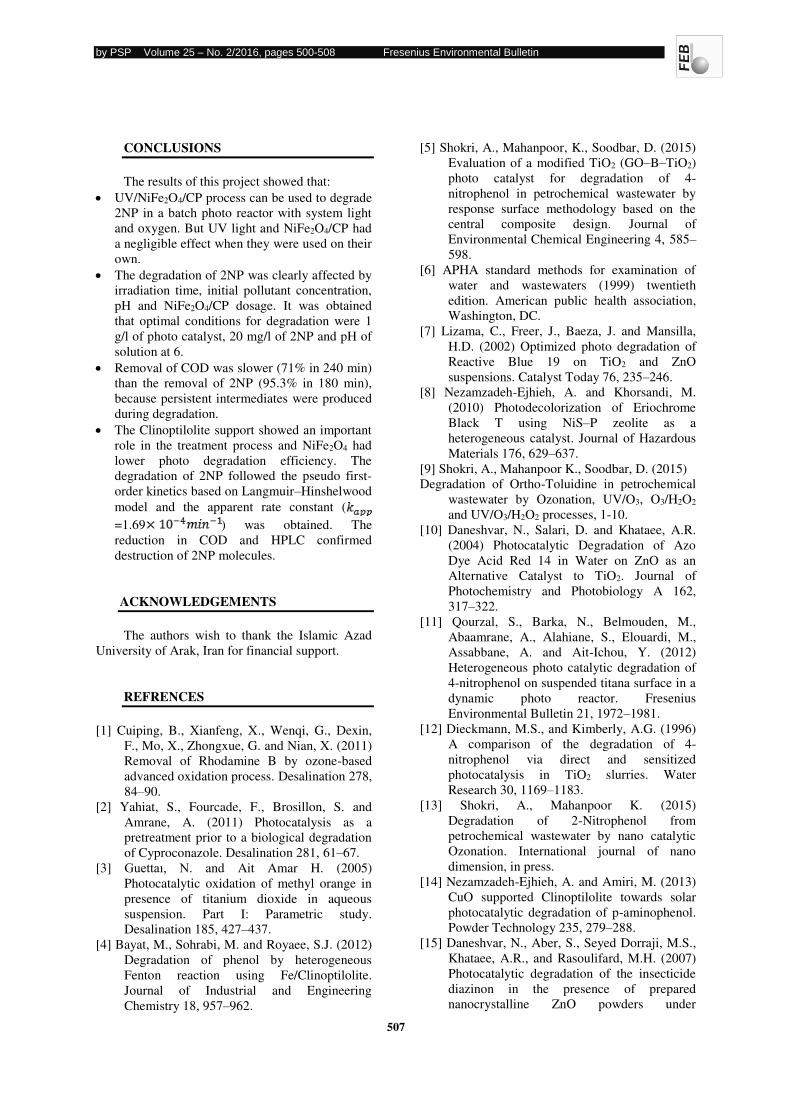
by PSP Volume 25 – No. 2/2016, pages 500-508 Fresenius Environmental Bulletin
507
CONCLUSIONS
The results of this project showed that:
UV/NiFe2O4/CP process can be used to degrade
2NP in a batch photo reactor with system light
and oxygen. But UV light and NiFe2O4/CP had
a negligible effect when they were used on their
own.
The degradation of 2NP was clearly affected by
irradiation time, initial pollutant concentration,
pH and NiFe2O4/CP dosage. It was obtained
that optimal conditions for degradation were 1
g/l of photo catalyst, 20 mg/l of 2NP and pH of
solution at 6.
Removal of COD was slower (71% in 240 min)
than the removal of 2NP (95.3% in 180 min),
because persistent intermediates were produced
during degradation.
The Clinoptilolite support showed an important
role in the treatment process and NiFe2O4 had
lower photo degradation efficiency. The
degradation of 2NP followed the pseudo first-
order kinetics based on Langmuir–Hinshelwood
model and the apparent rate constant (
=1.69 ) was obtained. The
reduction in COD and HPLC confirmed
destruction of 2NP molecules.
ACKNOWLEDGEMENTS
The authors wish to thank the Islamic Azad
University of Arak, Iran for financial support.
REFRENCES
[1] Cuiping, B., Xianfeng, X., Wenqi, G., Dexin,
F., Mo, X., Zhongxue, G. and Nian, X. (2011)
Removal of Rhodamine B by ozone-based
advanced oxidation process. Desalination 278,
84–90.
[2] Yahiat, S., Fourcade, F., Brosillon, S. and
Amrane, A. (2011) Photocatalysis as a
pretreatment prior to a biological degradation
of Cyproconazole. Desalination 281, 61–67.
[3] Guettaı, N. and Ait Amar H. (2005)
Photocatalytic oxidation of methyl orange in
presence of titanium dioxide in aqueous
suspension. Part I: Parametric study.
Desalination 185, 427–437.
[4] Bayat, M., Sohrabi, M. and Royaee, S.J. (2012)
Degradation of phenol by heterogeneous
Fenton reaction using Fe/Clinoptilolite.
Journal of Industrial and Engineering
Chemistry 18, 957–962.
[5] Shokri, A., Mahanpoor, K., Soodbar, D. (2015)
Evaluation of a modified TiO2 (GO–B–TiO2)
photo catalyst for degradation of 4-
nitrophenol in petrochemical wastewater by
response surface methodology based on the
central composite design. Journal of
Environmental Chemical Engineering 4, 585–598.
[6] APHA standard methods for examination of
water and wastewaters (1999) twentieth
edition. American public health association,
Washington, DC.
[7] Lizama, C., Freer, J., Baeza, J. and Mansilla,
H.D. (2002) Optimized photo degradation of
Reactive Blue 19 on TiO2 and ZnO
suspensions. Catalyst Today 76, 235–246.
[8] Nezamzadeh-Ejhieh, A. and Khorsandi, M.
(2010) Photodecolorization of Eriochrome
Black T using NiS–P zeolite as a
heterogeneous catalyst. Journal of Hazardous
Materials 176, 629–637.
[9] Shokri, A., Mahanpoor K., Soodbar, D. (2015)
Degradation of Ortho-Toluidine in petrochemical
wastewater by Ozonation, UV/O3, O3/H2O2
and UV/O3/H2O2 processes, 1-10.
[10] Daneshvar, N., Salari, D. and Khataee, A.R.
(2004) Photocatalytic Degradation of Azo
Dye Acid Red 14 in Water on ZnO as an
Alternative Catalyst to TiO2. Journal of
Photochemistry and Photobiology A 162,
317–322.
[11] Qourzal, S., Barka, N., Belmouden, M.,
Abaamrane, A., Alahiane, S., Elouardi, M.,
Assabbane, A. and Ait-Ichou, Y. (2012)
Heterogeneous photo catalytic degradation of
4-nitrophenol on suspended titana surface in a
dynamic photo reactor. Fresenius
Environmental Bulletin 21, 1972–1981.
[12] Dieckmann, M.S., and Kimberly, A.G. (1996)
A comparison of the degradation of 4-
nitrophenol via direct and sensitized
photocatalysis in TiO2 slurries. Water
Research 30, 1169–1183.
[13] Shokri, A., Mahanpoor K. (2015) Degradation of 2-Nitrophenol from
petrochemical wastewater by nano catalytic
Ozonation. International journal of nano
dimension, in press.
[14] Nezamzadeh-Ejhieh, A. and Amiri, M. (2013)
CuO supported Clinoptilolite towards solar
photocatalytic degradation of p-aminophenol.
Powder Technology 235, 279–288.
[15] Daneshvar, N., Aber, S., Seyed Dorraji, M.S.,
Khataee, A.R., and Rasoulifard, M.H. (2007)
Photocatalytic degradation of the insecticide
diazinon in the presence of prepared
nanocrystalline ZnO powders under
by PSP Volume 25 – No. 2/2016, pages 500-508 Fresenius Environmental Bulletin
508
irradiation of UV-C light. Separation and
Purification Technology 58, 91–98.
[16] Kasiri, M.B., Aleboyeh, H., and Aleboyeh A.
(2008) Degradation of Acid Blue 74 using Fe-
ZSM5 zeolite as a heterogeneous photo-
Fenton catalyst. Applied Catalysis B:
Environmental 84, 9–15.
[17] Jibril, B.Y., Atta, A.Y., Al-Waheibi, Y.M.,
and Al-Waheibi, T.K. (2012) Microwave-
enhanced catalytic degradation of 2-
nitrophenol on alumina-supported copper
oxides. Journal of Industrial and Engineering
Chemistry 26, 112–116.
[18] Byrappa, K., Subramani, A.K., Ananda, S.,
Lokanatha Rai, K.M., Dinesh, R.and
Yoshimura .M.(2006) Photocatalytic
degradation of Rhodamine B dye using
hydrothermally synthesized ZnO. Bulletin of
Materials Science 29, 433–438.
[19] Wang, G., Wu, F., Zhang, X., Lu, M. and
Deng N. (2006) Enhance photo catalytic
degradation of Bisphenol F by b-
Cyclodextrine in aqueous TiO2 dispersion.
Fresenius Environmental Bulletin 15, 61–67.
Received: 29.06.2015
Accepted: 26.12.2015
CORRESPONDING AUTHOR
*Corresponding Author E
Kazem Mahanpoor
Islamic Azad University
Department of Chemistry
Faculty of Science
Arak Branch, Arak – IRAN
e-mail: k- [email protected]
by PSP Volume 25 – No. 2/2016, pages 509-516 Fresenius Environmental Bulletin
509
MITROCHONDRIAL DNA CONTROL REGION POLYMORPHISMS OF LOGGERHEAD AND GREEN
TURTLES NESTING ON TURKISH BEACHES: QUICK RESULTS WITH RESTRICTION FRAGMENT LENGTH POLYMORPHISM (RFLP) ANALYSIS FOR
CONSERVATION ASSESSMENT
Arzu Kaska
Department of Science Education, Faculty of Education, Pamukkale University, Denizli, Turkey.
ABSTRACT
The genetic structures of two sea turtle species
(Caretta caretta and Chelonia mydas) nesting along
the Turkish coast, were analyzed using tissues
(kidney, liver, gonad, muscles etc.) from dead
hatchlings and embryos. We collected tissues 31
different (14 C. caretta and 17 C. mydas) dead
hatchlings from 10 different nesting beaches
(Dalyan, Dalaman, Fethiye, Çıralı, Belek, Kızılot, Anamur, Göksu, Kazanlı and Samandağ) and preserved in absolute alcohol. We used AluI,
HindII, HindIII, HaeIII and SmaI restriction
enzymes for digestion in PCR-RFLP analyses. The
SmaI and HindIII enzymes were not digested the
mtDNA from both species. We detected five
polymorphisms (in three C. caretta and two C.
mydas) on four different beaches of Turkey
(produced by the digestion of AluI and HindII
enzymes). These results showed that there are
genetical diversities of the sea turtle population on
Turkish beaches and these results are discussed in
identifying the genetic source of the turtles and
their conservation.
KEYWORDS:
Loggerhead turtle, green turtle, mitochondrial DNA,
Polymorphism, Restriction Fragment Length
Polymorphism.
INTRODUCTION
There are two species of sea turtles nesting in
the Mediterranean: the loggerhead turtle Caretta
caretta and the green turtle Chelonia mydas [1].
Both of these species are listed on Appendix 1 of
Conservation on International Trade in Endangered
Species of Wild Fauna and Flora (CITES),
prohibiting any international trade among
contracting parties such as International Union for
Conservation of Nature and Natural Resources
(IUCN). The loggerhead turtle is distributed in the
entire Mediterranean but the green turtle is nesting
in the Mediterranean is confined to Turkey, Cyprus,
Lebanon, Israel and Egypt [1, 2] having foraging
areas in Greece and Libya [3]. In Turkey, the green
turtle nesting is mostly confined to eastern beaches
whereas loggerhead turtles on the more western
beaches [4] (Figure 1).
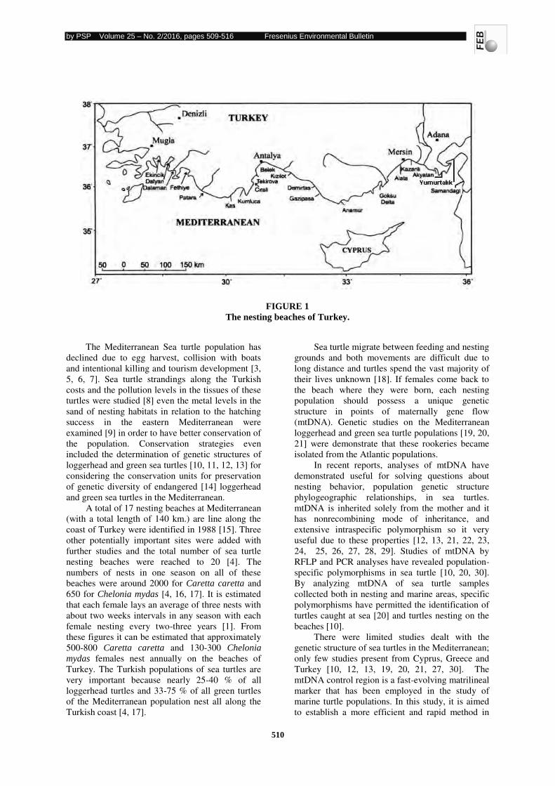
by PSP Volume 25 – No. 2/2016, pages 509-516 Fresenius Environmental Bulletin
510
FIGURE 1
The nesting beaches of Turkey.
The Mediterranean Sea turtle population has
declined due to egg harvest, collision with boats
and intentional killing and tourism development [3,
5, 6, 7]. Sea turtle strandings along the Turkish
costs and the pollution levels in the tissues of these
turtles were studied [8] even the metal levels in the
sand of nesting habitats in relation to the hatching
success in the eastern Mediterranean were
examined [9] in order to have better conservation of
the population. Conservation strategies even
included the determination of genetic structures of
loggerhead and green sea turtles [10, 11, 12, 13] for
considering the conservation units for preservation
of genetic diversity of endangered [14] loggerhead
and green sea turtles in the Mediterranean.
A total of 17 nesting beaches at Mediterranean
(with a total length of 140 km.) are line along the
coast of Turkey were identified in 1988 [15]. Three
other potentially important sites were added with
further studies and the total number of sea turtle
nesting beaches were reached to 20 [4]. The
numbers of nests in one season on all of these
beaches were around 2000 for Caretta caretta and
650 for Chelonia mydas [4, 16, 17]. It is estimated
that each female lays an average of three nests with
about two weeks intervals in any season with each
female nesting every two-three years [1]. From
these figures it can be estimated that approximately
500-800 Caretta caretta and 130-300 Chelonia
mydas females nest annually on the beaches of
Turkey. The Turkish populations of sea turtles are
very important because nearly 25-40 % of all
loggerhead turtles and 33-75 % of all green turtles
of the Mediterranean population nest all along the
Turkish coast [4, 17].
Sea turtle migrate between feeding and nesting
grounds and both movements are difficult due to
long distance and turtles spend the vast majority of
their lives unknown [18]. If females come back to
the beach where they were born, each nesting
population should possess a unique genetic
structure in points of maternally gene flow
(mtDNA). Genetic studies on the Mediterranean
loggerhead and green sea turtle populations [19, 20,
21] were demonstrate that these rookeries became
isolated from the Atlantic populations.
In recent reports, analyses of mtDNA have
demonstrated useful for solving questions about
nesting behavior, population genetic structure
phylogeographic relationships, in sea turtles.
mtDNA is inherited solely from the mother and it
has nonrecombining mode of inheritance, and
extensive intraspecific polymorphism so it very
useful due to these properties [12, 13, 21, 22, 23,
24, 25, 26, 27, 28, 29]. Studies of mtDNA by
RFLP and PCR analyses have revealed population-
specific polymorphisms in sea turtle [10, 20, 30].
By analyzing mtDNA of sea turtle samples
collected both in nesting and marine areas, specific
polymorphisms have permitted the identification of
turtles caught at sea [20] and turtles nesting on the
beaches [10].
There were limited studies dealt with the
genetic structure of sea turtles in the Mediterranean;
only few studies present from Cyprus, Greece and
Turkey [10, 12, 13, 19, 20, 21, 27, 30]. The
mtDNA control region is a fast-evolving matrilineal
marker that has been employed in the study of
marine turtle populations. In this study, it is aimed
to establish a more efficient and rapid method in
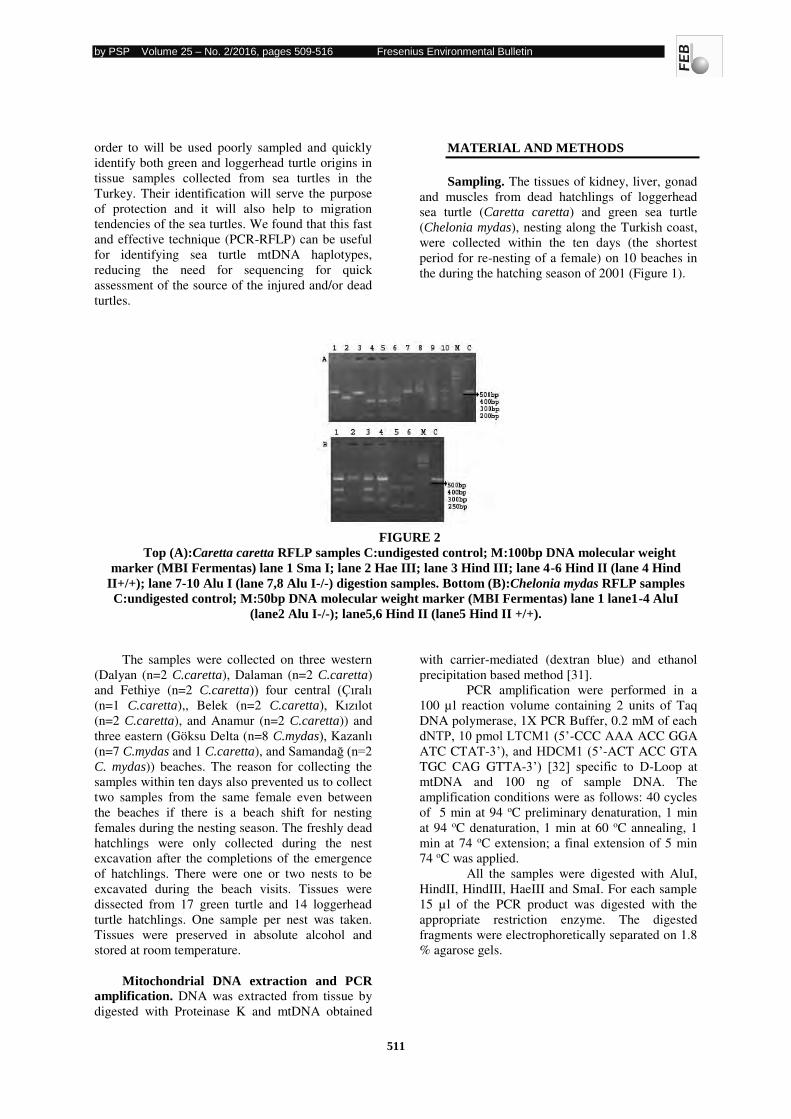
by PSP Volume 25 – No. 2/2016, pages 509-516 Fresenius Environmental Bulletin
511
order to will be used poorly sampled and quickly
identify both green and loggerhead turtle origins in
tissue samples collected from sea turtles in the
Turkey. Their identification will serve the purpose
of protection and it will also help to migration
tendencies of the sea turtles. We found that this fast
and effective technique (PCR-RFLP) can be useful
for identifying sea turtle mtDNA haplotypes,
reducing the need for sequencing for quick
assessment of the source of the injured and/or dead
turtles.
MATERIAL AND METHODS
Sampling. The tissues of kidney, liver, gonad
and muscles from dead hatchlings of loggerhead
sea turtle (Caretta caretta) and green sea turtle
(Chelonia mydas), nesting along the Turkish coast,
were collected within the ten days (the shortest
period for re-nesting of a female) on 10 beaches in
the during the hatching season of 2001 (Figure 1).
FIGURE 2
Top (A):Caretta caretta RFLP samples C:undigested control; M:100bp DNA molecular weight
marker (MBI Fermentas) lane 1 Sma I; lane 2 Hae III; lane 3 Hind III; lane 4-6 Hind II (lane 4 Hind
II+/+); lane 7-10 Alu I (lane 7,8 Alu I-/-) digestion samples. Bottom (B):Chelonia mydas RFLP samples
C:undigested control; M:50bp DNA molecular weight marker (MBI Fermentas) lane 1 lane1-4 AluI
(lane2 Alu I-/-); lane5,6 Hind II (lane5 Hind II +/+).
The samples were collected on three western
(Dalyan (n=2 C.caretta), Dalaman (n=2 C.caretta)
and Fethiye (n=2 C.caretta)) four central (Çıralı (n=1 C.caretta),, Belek (n=2 C.caretta), Kızılot (n=2 C.caretta), and Anamur (n=2 C.caretta)) and
three eastern (Göksu Delta (n=8 C.mydas), Kazanlı (n=7 C.mydas and 1 C.caretta), and Samandağ (n=2 C. mydas)) beaches. The reason for collecting the
samples within ten days also prevented us to collect
two samples from the same female even between
the beaches if there is a beach shift for nesting
females during the nesting season. The freshly dead
hatchlings were only collected during the nest
excavation after the completions of the emergence
of hatchlings. There were one or two nests to be
excavated during the beach visits. Tissues were
dissected from 17 green turtle and 14 loggerhead
turtle hatchlings. One sample per nest was taken.
Tissues were preserved in absolute alcohol and
stored at room temperature.
Mitochondrial DNA extraction and PCR
amplification. DNA was extracted from tissue by
digested with Proteinase K and mtDNA obtained
with carrier-mediated (dextran blue) and ethanol
precipitation based method [31].
PCR amplification were performed in a
100 µl reaction volume containing 2 units of Taq
DNA polymerase, 1X PCR Buffer, 0.2 mM of each
dNTP, 10 pmol LTCM1 (5’-CCC AAA ACC GGA
ATC CTAT-3’), and HDCM1 (5’-ACT ACC GTA
TGC CAG GTTA-3’) [32] specific to D-Loop at
mtDNA and 100 ng of sample DNA. The
amplification conditions were as follows: 40 cycles
of 5 min at 94 oC preliminary denaturation, 1 min
at 94 oC denaturation, 1 min at 60 oC annealing, 1
min at 74 oC extension; a final extension of 5 min
74 oC was applied.
All the samples were digested with AluI,
HindII, HindIII, HaeIII and SmaI. For each sample
15 µl of the PCR product was digested with the
appropriate restriction enzyme. The digested
fragments were electrophoretically separated on 1.8
% agarose gels.
by PSP Volume 25 – No. 2/2016, pages 509-516 Fresenius Environmental Bulletin
512
RESULTS
A PCR product of about 559 bp for green sea
turtle (Chelonia mydas) and 550 bp for loggerhead
sea turtle (Caretta caretta) from the control region
of mtDNA were obtained for both species. We used
AluI, HindII, HindIII, HaeIII and SmaI restriction
enzymes for digestion. No digestion products were
obtained for SmaI and HindIII. We did not find any
polymorphisms in HaeIII site and only AluI and
HindII enzymes were showed intra species
differences between the beaches for both species.
Most of the C. caretta specimens were
heteroplasmic as Alu I+/- , but only two C. caretta
showed homoplasmic pattern as Alu I-/-. These two
polymorphic specimens were obtained from one at
the western beach of Dalaman and the other one
from eastern beach of Kazanlı which is mainly used for green turtle nesting (Figure 1). For the enzyme
of Hind II, all loggerhead turtles showed
heteroplasmic (Hind II+/-) except for one which
found homoplasmic (Hind II+/+). This
homoplasmic specimen was obtained from Fethiye
beach which is at the west coast and nearly 45 km
away from Dalaman beach which also holds
another polymorphic pattern by Alu I. All the other
samples obtained from remain beaches showed the
pattern of Alu I+/- and Hind II+/-.
For C. mydas, majority of the samples showed
heteroplasmic (Alu I+/-), only one was found
homoplasmic (Alu I-/-). This polymorphic
specimen was obtained from Göksu Delta. Hind II
enzyme digested as heteroplasmic (Hind II+/-) in
most of the specimen, and only one found
homoplasmic (Hind II+/+). This homoplasmic
specimen were obtained sample from Samandağ Beach where end point of the eastern
Mediterranean. These two polymorphic sites were
nearly 200 km apart (Figure 1), the other samples
showed uniform pattern.
The mtDNA control region sequences were
obtained from the Gene Bank. The enzymes
restriction sites for loggerhead turtles were Alu I:
333-336; Hae III:428-431/490-493 and Hind
II:168-173 according to the sequence obtained from
Gene Bank Accession No I: U40435. These
sequences were chosen according to primers we
used and the restriction sites of the enzymes and the
fragment sizes we have obtained. Similarly, the
enzymes restriction sites for green turtles were Alu
I:337-340; Hind II:170-175 and Hae III:434-437
according to Gene Bank Accession Numbers of
U40435, M98394, S76889, Z50124 and Z50140.
DISCUSSION
Sea turtle research is generally focused on
nesting beaches, tagged and sampled. Genetic
studies were instigated to help fill this gap and
genetic diversity and structuring of the populations
are important for understanding loggerhead and
green turtle life history their management and
conservation purposes. The loggerhead and green
sea turtles are widely distributed species especially
in the Mediterranean beaches. According to the
IUCN [14], C. mydas is categorized as Endangered
and C.caretta is Vulnerable as a result of egg
harvest, incidental mortality relating to marine
fisheries, degradation of nesting habitats and
tourism development. Therefore, in addition to
conventional conservation actions, additional
information such as genetic structure of populations
is required for determination of conservation.
Molecular markers, such as n DNA and mt DNA
sequences are of great importance for the
description of genetic structure of turtle populations
A generational time scale, involving change
from one generation to the other, is a dynamic
process but operates within relatively narrow
morphological constraints compared to the time
available for change [33]. Bowen et al. [34] studied
the Ridley sea turtles and compared mtDNA control
region among 89 Ridley turtles, including the sole
L. kempi and L. olivacea nesting population. They
also reported that the haplotype differences within
these populations might occurred within the last
300.000 years by molecular clock estimations. Sea
turtles might have colonized the Mediterranean
during the most recent glacial period (18.000 to
12.000 years before the present) as proved by
genetical study [10]. The green turtles are only
colonized on the eastern beaches of Turkey close to
Cyprus. The loggerhead turtles are mainly nesting
most south western beaches but few numbers are
also present on these green turtle nesting beaches.
The origin of colonization of the species to the
Mediterranean beaches can also be understood by
looking at the genetical diversity or similarity of
these species. This information may also help to
understand the approximate age of the beach and
therefore the colonization order of the sea turtles on
these beaches. Lahanas et al. [35] also studied green
turtle genetic structure by control region sequences
of mtDNA and found variations both within and
between four nesting populations. Another study
with Encalada et al. [19] found 18 haplotypes
among 147 individuals from nine nesting
populations in the world, by sequencing the
mtDNA control region. They described the C.
mydas from Cyprus holding the Haplotype XIII
except for heteroplasmy at site 167. This was later
by PSP Volume 25 – No. 2/2016, pages 509-516 Fresenius Environmental Bulletin
513
proved by Kaska [12]. In addition to these mtDNA
haplotypes, three new haplotypes (CM-A61, CM-
A62 and CM-A63) were described recently [21].
There were a few main studies on the
loggerhead genetical structure from Turkish
beaches [20, 27, 30]. Schroth et al. [30] in the
study of loggerhead turtle's mtDNA sequence
analyses in the Eastern Mediterranean, found 11
haplotypes in 81 individuals including from
Turkey. They also found that haplotype III, which
was only found in Turkey, is significantly
decreasing from western towards eastern beaches.
Their study also showed that there are genetic
differences both between coastal areas and
neighboring nesting beaches. The results of Alu-/-
for loggerhead turtle specimens (Haplotype III of
Schroth et al. [30]) were also found in our study
which confirms the presence of this haplotype on
both at the western beach (Dalaman) and eastern
beach (Kazanlı). Schroth et al. [30] reported that the
frequency was 42 % at the western beaches (Dalyan
and Fethiye) and decreased towards to east (i. e., 16
% in Anamur) but there were no samples taken by
them from east of Anamur beach. The presence of
this haplotype in Kazanlı also showed that this
haplotype is one of the most common one, may be
the oldest haplotype, in Turkey.
In many studies involving analysis of mtDNA,
one or several haplotype groups of the species
distribution are frequently observed [13, 21, 27].
Carreras et al. [13] studied the loggerhead sea
turtle's genetic structure in the eastern
Mediterranean. They reported a total of five
haplotypes. Two haplotypes of them (Haplotypes
CC-A2 and CC-A3) were previously described both
the Mediterranean and Atlantic nesting beaches [11,
20]. They reported mt DNA sequencing differences
between eastern and western rookeries. The results
were also found in our study which confirms
differences for mtDNA have been found between
eastern and western rookeries. Another studies
involving analysis of mtDNA [27]. In this study
Yılmaz et al. [27] detected 7 different haplotypes by mtDNA and microsatellite analyses. They were
described Haplotypes CC-A52.1, CC-A53.1 and a
variant of the CC-A3. Haplotype CC-A3.2, for first
time in their work. Their results showed that
Turkish C. caretta have a high genetic diversity in
the Mediterranean and Turkish nesting sites could
be distinguished as five management units. In
recent years, Bağda et al. [21] studied green turtle's genetic structure from Turkey and Northern Cyprus
beaches. Tissues were collected on six beaches
from 256 different nests. They found 859 bp
fragment of control region from six distinct mtDNA
haplotypes. Three of them described for the first
time in their study (haplotypes CM-A61, CM-A62
and CM-A63). As mentioned above Haplotypes
CM-A13 and CM-A14 had been previously
reported from the Cyprus [12, 19]. Haplotype CM-
A27, reported from a foraging ground of North
Carolina and Cuba [36] were recorded for the first
time in the Mediterranean [21]. Bağda et al. [21] found three heteroplasmic individuals from
Akyatan (haplotypes, CM-A13/CM-A27),
Samandag (haplotypes, CM-A13/CM-A63) and
Yumurtalık (haplotypes, CM-A13/CM-A61)
nesting populations. Our results of two
polymorphisms (Alu I-/-, Hind II+/+), present in
green turtles, suggesting that there is definitely
more than one (Haplotype XIII) haplotype as
described by Encalada et al. [19] and Kaska [12].
Our results of Hind II+/+ confirms the presence of
the Haplotype XIII on Samandağ beach but the
other one with Alu I-/- from Göksu Deltası implies the presence of other haplotype in Turkey. The
nesting sites of green turtles are only found in the
eastern Mediterranean, our results suggested that
there may be genetically differences between the
females nesting on very close beaches. These
probably need to be better determined by analyzing
more samples and sequencing the mtDNA control
regions. The similar polymorphisms found on
loggerhead turtles are also suggesting that there are
definitely some genetic differences between the
beaches that far from each other (i.e., Dalaman and
Kazanlı) and also close beaches (i.e., Dalaman and Fethiye). One possible explanation of these results
might be the time in difference in occurrence of
these beaches during the post-glacial period in
Mediterranean. The most eastern beaches might
occur first and western ones might follow.
Discussion on the effects of global warming on sea
turtle populations has focused on loss of nesting
beach habitat as a result of sea level rise and on
skewed sex ratios as an effect of temperature
increases on temperature-dependent sex
determination. One of the places that the largest
environmental changes are expected to occur
around the Mediterranean [37]. These climatic
changes, in the eastern Mediterranean, may have
altered circulation patterns [38] and affected the
deep-sea ecosystem [39]. Therefore, the
Mediterranean Sea turtle population may be the
first to be impacted by climatic changes. From this
perspective, those beach that holding the
genetically different populations would gain
additional importance in helping this species to
survive in the Mediterranean.
According to the numbers of nests recorded on
beaches according the studies so far, The mean
annual loggerhead turtle nest numbers were found
on Belek and Dalyan beaches were somehow
around 2-300 and higher. All the 4 loggerhead
by PSP Volume 25 – No. 2/2016, pages 509-516 Fresenius Environmental Bulletin
514
samples that collected from these beaches showed
uniform pattern. The mean annual numbers of nests
on Dalaman, Fethiye, Anamur and Kızılot beaches
were around 100. Two of the samples from these
beaches (one from Fethiye and another from
Dalaman) were found to be different than the
others. The numbers of loggerhead turtle nests per
year were very few or around 50 on Cirali and
Kazanli beaches and one sample obtained from
Kazanli were also found to be different. The
number of green turtle nests on three nesting
beaches seems to be similar and may hold around
1-200 nests per year. The one of samples obtained
from Samandag and Goksu Delta beaches were
found to be genetically different.
For an endangered species, researchers are
now trying to give priority to protect the beaches
holding more nests [40] , more data accumulation
by completing these genetical studies, we may
concentrate to protect genetically distinct
populations on the beaches despite of the less
number of nests. Recently, potential declines in sea
turtle nesting population have shown to be
declining on one of the Turkish beaches [2]. The
differences in genetic structures may serve as
genetic tags to identify found dead stranded on the
beaches due to drawn in fishing trawls and they can
be addressed at the beaches. This may highlight a
new approach to species conservation especially
protected under several conventions. The impacts
of climate change, such as changes in nesting beach
physiochemical characteristics and the implications
for nesting, modeling of predicted beach loss under
various sea level rise scenarios, and the possible
secondary beaches and their genetic diversity might
increase the importance in the future. Both the
nesting females on the beaches and the juveniles
and the adults of the both sexes in the sea should be
studied in terms of genetic diversity by getting
more DNA samples in order to find out more
precise information regarding the genetic
composition of sea turtles in the eastern
Mediterranean.
Understanding turtles migration routes, the
impact of human activities environmental
conditions on them essential for the development of
practical conservation measures. The long
generation time of sea turtles make them especially
vulnerable to decrease. Mitochondrial DNA or
nuclear DNA sequencing techniques were used in
identifying the genetic diversity present between
the sea turtle population of Turkish beaches. In
some cases the sample may be analyzed in a quick
way in order to identify the beach source of
specimens that found injured and/or dead.
ACKNOWLEDGEMENTS
This work was granted by Pamukkale
University Research Fund as PAU-2002-FBE-001.
I would like to thank Prof. Dr. Huseyin Bağcı for his supervision of my Master Thesis. I am also
grateful to Dr. İbrahim Açıkbaş for the lab work.
REFERENCES
[1] Groombridge, B. (1990). Marine turtles in the
Mediterranean: Distribution, population status,
conservation: A report to the Council of
Europe, World. Conservation Monitoring
Centre, Cambridge U.K. 72p.
[2] Ilgaz, Ç., Türkozan,·O., Özdemir, A., Kaska,
Y. and Stachowitsch (2007). Population
decline of loggerhead turtles: two potential
scenarios for Fethiye beach, Turkey.
Biodiversity and Conservation.
[3] Casale, P. and Margaritoulis, D. (2010). Sea
turtles in the Mediterranean: distribution,
threats and conservation priorities. IUCN
Gland Switzerland.
[4] Turkozan, O. and Kaska, Y. (2010). Turkey.
In:Casale, P., Margaritoulis, D. (Eds), Sea
turtles in the Mediterranean: Distribution,
Threats and Conservation Prioritiess.
IUCN/SSC Marine Turtle SPecialist Group,
Gland; Switzerland. pp, 257-293.
[5] Margaritoulis, D., Argano, R., Baran, I.,
Bentivegna, F., Bradai, M.N., Caminas, J.A.,
Casale, P., De Metrio, G., Demetropoulos, A.,
Gerosa, G. et al. (2003). Loggerhead turtles in
the Mediterranean Sea: present knowledge and
conservation perspectives. In: Bolten AB,
Witherington BE (eds) Loggerhead sea turtles,
Washington, USA, 340 pp 175–198.
[6] Tomas, J., Gozalbes, P., Raga, J.A. and Godley,
B.J. (2008). By catch of loggerhead sea
turtles: insights from 14 years of stranding
data. Endangered Species Research 5, 161-
169.
[7] Casale, P. (2011). Sea turtle by-catch in the
Mediterranean. Fish and Fish. 12, 299-316.
[8] Kaska, Y., Çelik, A., Bağ, H., Aureggi, M., Özel, K., Elçi, A., Kaska, A. and Elçi, L.
(2004). Heavy metal monitoring in stranded
sea turtles along the Mediterranean coast of
Turkey. Fresenius Env. Bul 13, 769-776.
[9] Yalçın Özdilek, S., Özdilek, H.G. and Sangun M.K. (2006). The effect of some elements
(Ca, Mg and Cr) on the nesting activity of
green turtles on the Samandağ Beach, Turkey. Fresenius Env. Bul 15, 1607-1615.
by PSP Volume 25 – No. 2/2016, pages 509-516 Fresenius Environmental Bulletin
515
[10] Bowen, B.W., Avise, J.C., Richardson, J.I.,
Meylan, A.B., Margaritoulis, D. and Hopkins-
Morphy, S.R. (1993). Population structure of
loggerhead turtles (Caretta caretta) in the
Northwestern Atlantic Ocean and
Mediterranean Sea. Conserv Biol 7, 834-844.
[11] Encalada, S.E., Bjorndal, K.A., Bolten, A.B.,
Zurita, C.J., Schroeder, B., Possardt, E., Sears,
C.J., Bowen, B.W. (1998). Population
structure of loggerhead turtle (Caretta caretta)
nesting colonies in the Atlantic and
Mediterranean as inferred from mitochondrial
DNA control region sequences. Mar. Biol.
130, 567-575.
[12] Kaska, Y. (2000). Genetic structure of
Mediterranean sea turtle populations. Turk J
Zool 24, 191-197.
[13] Carreras, C.; Pascual, M.; Cardona, L.,
Aguilar, A.; Margaritoulis, D.; Rees, A.;
Turkozan, O.; Levy., Y., Gasith, A., Aureggi,
M., and Khalil, M. (2007). The genetic
structure of the loggerhead sea turtle (Caretta
caretta) in the mediterranean as revealed by
nuclear and mitochondrial DNA and its
conservation implications. Conserv Genet 8,
761-775.
[14] IUCN. (2014). The IUCN Red List of
Threatened Species. Version 2014.3.
<www.iucnredlist.org>. Downloaded on 14
January 2015.
[15] Baran, İ. and Kasperek, M. (1989). Marine
turtles, Turkey, status survey 1988 and
recommendation for conservation and
management. Prepared by WWF Heidelberg
129 pp.
[16] Canbolat, A.F. (2004). A review of sea turtle
nesting activity along the Mediterranean coast
of Turkey. Biological Conservation 116, 81-
91.
[17] Kaska, Y., Baran, I., Ilgaz, Ç., Türkozan, O.,
Öz, M. and Erdoğan, A. (2005). An estimation
of the total nesting activity of sea turtles in
Turkey, Pp. 204-205 In: Coyne M.S., and
Clark, R.D. (Compilers). Proceedings of the
Twenty-First Annual Sea Turtle Biology and
Conservation. NOAA Technical
Memorandum NMFS-SEFCS-528, Miami,
368 pp.
[18] Carr, A. (1980). Some problems of sea turtle
ecology. Amer Zool 20, 489-498.
[19] Encalada, S.A., Lahanas, P.N., Bjorndal,
K.A., Bolten, A.B., Miyamoto, M.M. and
Bowen, B.W. (1996). Phylogeography and
population structure of the Atlantic and
Mediterranean green turtle, Chelonia mydas, a
mitochondrial DNA control region sequence
assessment. Mol Ecol 5, 473-483.
[20] Laurent, L., Casale, P., Bradai, M.N., Godley,
B.J., Gerosas, G., Broderick, A.C., Schroth,
W., Schierwater, B., Levy, A.M., Freggi, D. et
al. (1998). Molecular resolution of marine
turtle stock composition in fishery bycatch, a
case study in the Mediterranean. Mol Ecol 7,
1529-1542.
[21] Bağda, E., Bardakçı, F. and Türkozan, O. (2012). Lower genetic structuring in
mitochondrial DNA than nuclear DNA among
the nesting colonies of green turtles (Chelonia
mydas) in the Mediterranean. Biochemical
Systematics and Ecology 43, 192-199.
[22] Moritz, C., Dowling, T.E. and Brown, W.M.
(1987). Evolution of animal mitochondrial
DNA: relevance for population biology and
systematic. Ann Rev Ecol Syst 18, 269-292.
[23] Avise, J.C., Bowen, B.W., Lamb, T., Meylan,
A.B. and Bermingham, E. (1992).
Mitocondria; DNA evolution at a turtle's pace:
Evidence for low genetic variability and
reduced microevolutionary rate in the
Testudines. Mol Biol Evol 9, 457-473.
[24] Rand, D.M. and Kann, L.M. (1998). Mutation
and selection at silent and replacement sites in
the evolution of animal mitochondrial DNA.
Genetica 102-103, 393-407.
[25] Solignac, M . (2004). Mitochondrial DNA in
the Drosophila melanogaster Complex.
Genetica 120 (1-3), 41-50.
[26] Bourjea, J., Lapegue, S., Gagnevin, L.,
Broderick, D., Mortimer, A., Ciccione, S.,
Roos, D., Taquet, C. and Grizel, H. (2007).
Phylogeography of the green turtle, Chelonia
mydas, in the Soutwest Indian Ocean.
Molecular Ecology, 16, 175-186.
[27] Yılmaz, C., Türkozan, O. and Bardakçı, F. (2011). Genetic structure of loggerhead turtle
(Caretta caretta) populations in Turkey.
Biochemical Systematics and Ecology 39,
266-276.
[28] Garofalo, L., Mastrogiacomo, A., Casale, P.,
Carlini, R., Eleni, C., Freggi, D., Gelli, D.,
Knittweis, L., Mifsud, C., Mingozzi, T. et al.
(2013). Genetic characterization of central
Mediterranean stocks of the loggerhead turtle
(Caretta caretta) using mitochondrial and
nuclear markers, and conservation
implications. Aquat Conserv.
doi:10.1002/aqc.2338.
[29] Shamblin, B.M., Bolten, A.B., Abreu-Grobois,
F.A., Bjorndal, K.A., Cardona, L., Carreas, C.,
Clusa, M., Monzon-Argello, C., Nairn, C.J.
and Nielsen, J.T. (2014). Geographic patterns
of genetic variation in a broadly distributed
marine vertebrate: new insights into
by PSP Volume 25 – No. 2/2016, pages 509-516 Fresenius Environmental Bulletin
516
loggerhead turtle stock structure from
expanded mitochondrial DNA sequences. Plos
One 9.
[30] Schroth, W., Streit, B. and Schierwater, B.
(1996). Evolutionary handicap for turtles.
Nature 384, 521-522.
[31] Kalmar, T., Bachrati, C.Z., Marcsik, A. and
Rasko, I. (2000). A Simple and Efficient
Method for PCR Amplifiable DNA Extraction
from Ancient Bones, Nucleic Acids Res.
28(12), e67(I-IV).
[32] Allard, M.W., Miyamoto, M.M., Bjorndal,
K.A., Bolten, A.B. and Bowen, B.W. (1994).
Support for natal homing in green turtles from
mitochondrial DNA sequences. Copeia
1994(1),34-41.
[33] Gingerich, P.D. (2001). Rates of evolution on
the time scale of the evolutionary process.
Genetica 112-113, 127-144.
[34] Bowen, B.W., Clark, A.M., Abreu-Grobois,
F.A., Chaves, A., Reichart, R.A. and Ferl, R.J.
(1997). Global phylogeography of the ridley
sea turtles (Lepidochelys spp.) as inferred
from mitochondrial DNA sequences. Genetica
101(3), 179-189.
[35] Lahanas, P.N., Miyamota, M.M., Bjorndal,
K.A. and Bolten, A.B. (1994). Molecular
evolution and population genetics of Greater
Caribbean green turtles (Chelonia mydas) as
inferred from mitochondrial DNA control
region sequences. Genetica 94, 57-67.
[36] Naro-Maciel, E., Becker, J.H., Lima,
E.H.S.M., Marcovaldi, M.A. and DeSalle, R.
(2007). Testing dispersal hypotheses in
foraging green sea tutrles (Chelonia mydas) of
Brazil. J. Hered 98, 29-39.
[37] Nicholls, R.J., Hoozemans, F.M.J. and
Marchard, M. (1999). Increasing food risk and
wetland losses due to global sea-level rise:
regional and global analyses. Glob En
Changes 9, 69-87.
[38] Roether, W., Manca, B.B., Klein, B., Bregant,
D., Georgopoulos, D., Beitzel, V., Kovacevic,
V. and Luchetta, A. (1996). Recent changes in
eastern Mediterranean deep waters. Science
271, 333-335.
[39] Danovaro, R., Dell’Anno, A., Fabiano, M., Pusceddu, A. and Tselepides, A. (2001).
Deep-sea ecosystem response to climate
changes: the eastern Mediterranean case study.
Trends in Ecol Evol 16(9), 505-510.
[40] Başkale, E. and Kaska, Y. (2005). Sea Turtle
Nest Conservation Techniques on
Southwestern Beaches in Turkey. Isr J Zool
51, 13-26.
Received: 03.07.2015 Accepted: 06.01.2016
CORRESPONDING AUTHOR
Arzu Kaska Department of Science Education
Faculty of Education
Pamukkale University
Kınıklı-Denizli – TURKEY
e-mail: [email protected]
by PSP Volume 25 – No. 2/2016, pages 517-524 Fresenius Environmental Bulletin
517
EFFECTS OF LOW MOLECULAR WEIGHT ORGANIC ACIDS
ON PHOSPHORUS ADSORPTION CHARACTERISTICS IN A
BLACK CLAY SOIL IN NORTHEAST CHINA
Yongzhuang Wang1,2,3, Baoqing Hu1,2, Yan Yan1,2,*
1 Key Laboratory of Environment Change and Resources Use in Beibu Gulf, Guangxi Teachers Education University, Ministry of
Education, Nanning 530001, China
2 Guangxi Key Laboratory of Earth Surface Processes and Intelligent Simulation, Guangxi Teachers Education University, Nanning 530001,
China
3 College of Environment and Life Science, Guangxi Teachers Education University, Nanning 530001, China
ABSTRACT
The decrease of P adsorption induced by low
molecular weight organic acids (LMWOA) is
considered as an important mechanism for enhancing
P mobilization in soils. But how LMWOA
specifically alter soil P adsorption capacity is not well
understood, much less the mechanisms involved. In
this study, the effects of three common LMWOA
(oxalic acid, citric acid and malic acid) on P
adsorption in a black clay soil were studied in batch
experiments, followed by sequential P fractionation to
elucidate the mechanisms of P adsorption perturbed
by LMWOA. The adsorption data of the studied soil
were well fitted to Freundlich equation
(r2=0.821-0.878, P<0.01). Oxalic acid, citric acid and
malic acid at 10 mmol kg-1 soil decreased Freundlich
parameters Kf and n, which represent P adsorption
capacity and energy. The mechanism involved is that
LMWOA significantly decreased the amounts of P
adsorbed in soil NaHCO3-Pi (soil soluble and
exchangeable Pi, 11.6-29.3%) and NaOH-Pi (Fe/Al-Pi,
18.3-41.2%) fractions.
KEYWORDS: Inorganic P fraction; Organic P fraction; Sequential
extraction; Batch experiments; Mechanisms
INTRODUCTION
To overcome phosphorus (P) deficiency,
exudation of low molecular weight organic acids
(LMWOA) from roots is a common plant strategy that
mobilizes unavailable P in soils [1, 2]. The decrease
of P adsorption induced by LMWOA is considered as
an important mechanism for enhancing P mobilization
in soils. Among various LMWOA, oxalic acid, citric
acid and malic acid are three common organic acids
exuded from plant roots and identified in soils, and
they vary in their effectiveness in mobilizing soil P
for plants uptake [3, 4]. Though concentrations of
LMWOA in soil are very low (10-3 to 10-5 mol L-1),
these acids may accumulate to levels toxic to plant
growth and threatening to environment under suitable
environmental conditions [5]. The ability of the
LMWOA to reduce P adsorption results in a larger
pool of P in soil solution that enhances P acquisition.
However, this large amount of P in soil solution that
results from the release or removal from solid (e.g.
soil minerals, organic matter and limestone) has
potential to increase the risk of P loss to overland and
subsurface flow, exacerbating eutrophication of
freshwaters [6-8]. Therefore, better preventing and
controlling P loss risk could be achieved by a greater
understanding of how LMWOA specifically alter soil
P adsorption capacity and the mechanisms involved.
Soil P adsorption capacity is a function of factors
such as the Fe/Al oxides contents, exchangeable Ca
/Mg concentrations, soil texture, porosity, pH, ionic
strength and hydraulic conductivity [9]. While
LMWOA may have reduced P adsorption through
interactions with calcium carbonates and Fe/Al oxides,
why the response varied depending on the type of
LMWOA needs to be explained. The objective of the
present study was therefore to study the impacts of
oxalic acid, citric acid and malic acid on P adsorption
characteristics in a black clay soil in Northeast China.
The mechanisms involved were elucidated by
sequential P fractionation after batch adsorption
experiments.
MATERIALS AND METHODS
Soils. Samples of the topsoil (0-20cm) were
collected from Hailun (47°26’N, 126°38’E) Experimental Stations of Ecology, Chinese Academy
of Sciences. The climate at the site is continental
monsoon, characterized by warm-wet summer and
dry-cold winter. The mean annual temperature is 2°C,
frost-free period 120 days and annual precipitation
500-600 mm. The test soil was a major soil type for
agricultural production in the local area. Soil samples
by PSP Volume 25 – No. 2/2016, pages 517-524 Fresenius Environmental Bulletin
518
were air dried and ground to pass through a 2-mm
sieve before use. Selected chemical and physical
properties are shown in Table1.
Batch experiments. Triplicate soil samples (3 g)
were placed in 50 ml centrifuge tubes, and then 30 ml
of 0.01M KCl solution containing 0-50 mg P L-1 as
KH2PO4 and 0 mmol LMWOAs kg-1 soil (control)
or 0-50 mg P L-1 as KH2PO4 plus 10 mmol
LMWOAs kg-1 soil was added to each tube. This
resulted in a total of 72 centrifuge tubes that received
6 levels of P (0, 10, 20, 30, 40 and 50 mg P L-1)
combined with four treatments (control, oxalic acid,
citric acid and malic acid) from a P-LMWOAs
solution. The concentration of LMWOA was chosen
by considering the values of organic acids in soil
extracts [10, 11]. Two drops of toluene were added to
each tube to inhibit microbial activity prior to capping
the tube. All centrifuge tubes were shaken on an
end-to-end shaker (15-cycles min-1) for 24 h at
25±1°C. The suspensions were centrifuged at
12000×g for 10 min and filtered through Whatman
filter paper (No.42). The P concentration of the
filtrate was determined colorimetrically with the
molybdate-blue method [12]. The adsorption of added
P was calculated as the difference between the
concentration of soluble P added in the initial solution
and P in equilibrium solution after 24 h. P adsorption
parameters were calculated using Langmuir,
Freundlich and Linear equations as described below.
Langmuir equation. The P adsorption parameters
were calculated using the linear form of transformed
adsorption isotherms of Langmuir Equation:
C/X=(C/Xmax) +1/ (K Xmax), (1)
where C is the concentration of P in equilibrium
solution (mg P L-1), X is the amount of P adsorbed by
soil (mg P kg-1), Xmax is the Langmuir P adsorption
maxima (mg P kg−1), and K is an affinity constant related to the binding energy (L mg−1). Model
parameters were fit from a linear regression of C/X against C, where the slope equals 1/Xmax and the
intercept equals 1/ (K Xmax ).
Freundlich equation. The P adsorption
parameters were calculated using the linear form of
the Freundlich equation:
Log X=log Kf +1/n log C, (2)
where X is the amount of P adsorbed (mg kg-1
soil), C is the equilibrium concentration of P (mg L-1),
and Kf and n are constants related to the sorption
capacity and bonding energy, and the linear
regression of log C against log X gives a regression
coefficient, a slope of 1/n and an intercept of log Kf.
Linear equation. The linear equation has the
form:
X=a + b C, (3)
where X is the amount of P adsorbed (mg kg-1
soil), C is the equilibrium concentration of P (mg L-1).
The parameter b represents the buffering capacity
(EBC) of the equation.
Soil P fractionation. Soil samples before and
after the batch P adsorption experiments were
extracted using the Hedley P fractionation procedure
[13], with modifications as proposed by Kang et al.
[14]. Specifically, 0.5 g of soil samples were
subjected to sequential extraction with 30 ml 0.5 mol
L-1 NaHCO3 (pH=8.5) for labile inorganic P (Pi) and
organic P (Po) fractions, 30 ml 0.1 mol L-1 NaOH for
Fe-/Al-bound Pi and Po fractions, 30 ml 1.0 mol L-1
HCl for Ca-bound Pi fraction. After these extractions,
the remaining residue was subjected to digestion with
10 ml H2SO4+ 0.5 ml HClO4 at 360 °C, which
extracts the soil redual Pi and Po. The extracted Pi
collected at each step was analyzed colorimetrically
with the molybdate-blue method. Total Pi in the
NaHCO3 and NaOH extracts was determined by
digesting in autoclave (103.4 K Pa, 121 °C) with
acidified potassium persulfate (K2S2O8). The Po in
the NaHCO3 and NaOH fractions was calculated as
the difference between total and inorganic P.
Statistical analysis. After fitting P adsorption
data to linear forms of the Langmuir, Freundlich and
Linear equations, least-square-regression analysis was
used to determine the slope and intercept of the
best-fit model for P-adsorption in each of the studied
soils. All data on soil fractionated P were expressed as
the average amounts of P adsorbed among the
equilibrated (24 h) P solutions (0-50 mg P L-1). Soil
P fractions were subject to the normality and
homogeneity tests before analysis of variance
(ANOVA) using SAS statistical package (SAS 9.1).
One-way analysis of variance (ANOVA) was used to
determine the effects of control, oxalic acid, citric
acid and malic acid on each fractionated P. Least
significant difference (LSD) was conducted only
when the analysis of variance was significant at p <
0.05.
RESULTS AND DISCUSSION
Batch experiments. Data on the adsorption of
added P from P-LMWOAs solutions in the studied
soils fitted better to the Freundlich equation
(r2=0.821-0.878, p<0.01) than the Linear
(r2=0.423-0.797) and Langmuir (r2=0.075-0.742)
equations (Table 2).
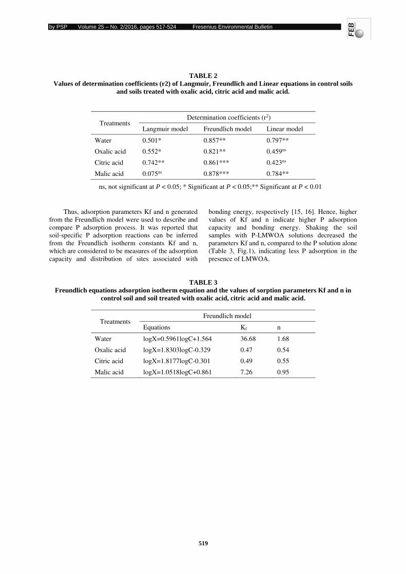
by PSP Volume 25 – No. 2/2016, pages 517-524 Fresenius Environmental Bulletin
519
TABLE 2
Values of determination coefficients (r2) of Langmuir, Freundlich and Linear equations in control soils
and soils treated with oxalic acid, citric acid and malic acid.
ns, not significant at P < 0.05; * Significant at P < 0.05;** Significant at P < 0.01
Thus, adsorption parameters Kf and n generated
from the Freundlich model were used to describe and
compare P adsorption process. It was reported that
soil-specific P adsorption reactions can be inferred
from the Freundlich isotherm constants Kf and n,
which are considered to be measures of the adsorption
capacity and distribution of sites associated with
bonding energy, respectively [15, 16]. Hence, higher
values of Kf and n indicate higher P adsorption
capacity and bonding energy. Shaking the soil
samples with P-LMWOA solutions decreased the
parameters Kf and n, compared to the P solution alone
(Table 3, Fig.1), indicating less P adsorption in the
presence of LMWOA.
TABLE 3
Freundlich equations adsorption isotherm equation and the values of sorption parameters Kf and n in
control soil and soil treated with oxalic acid, citric acid and malic acid.
Treatments Freundlich model
Equations Kf n
Water logX=0.5961logC+1.564 36.68 1.68
Oxalic acid logX=1.8303logC-0.329 0.47 0.54
Citric acid logX=1.8177logC-0.301 0.49 0.55
Malic acid logX=1.0518logC+0.861 7.26 0.95
Treatments Determination coefficients (r2)
Langmuir model Freundlich model Linear model
Water 0.501* 0.857** 0.797**
Oxalic acid 0.552* 0.821** 0.459ns
Citric acid 0.742** 0.861*** 0.423ns
Malic acid 0.075ns 0.878*** 0.784**
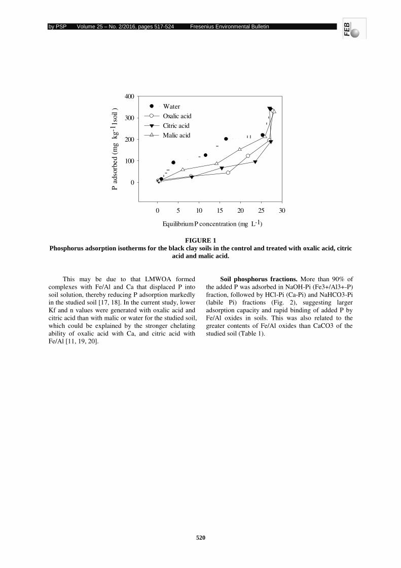
by PSP Volume 25 – No. 2/2016, pages 517-524 Fresenius Environmental Bulletin
520
Equilibrium P concentration (mg L-1)
0 5 10 15 20 25 30
P a
dso
rbed (
mg
kg
-11so
il )
0
100
200
300
400
Water
Oxalic acid
Citric acid
Malic acid
FIGURE 1
Phosphorus adsorption isotherms for the black clay soils in the control and treated with oxalic acid, citric
acid and malic acid.
This may be due to that LMWOA formed
complexes with Fe/Al and Ca that displaced P into
soil solution, thereby reducing P adsorption markedly
in the studied soil [17, 18]. In the current study, lower
Kf and n values were generated with oxalic acid and
citric acid than with malic or water for the studied soil,
which could be explained by the stronger chelating
ability of oxalic acid with Ca, and citric acid with
Fe/Al [11, 19, 20].
Soil phosphorus fractions. More than 90% of
the added P was adsorbed in NaOH-Pi (Fe3+/Al3+-P)
fraction, followed by HCl-Pi (Ca-Pi) and NaHCO3-Pi
(labile Pi) fractions (Fig. 2), suggesting larger
adsorption capacity and rapid binding of added P by
Fe/Al oxides in soils. This was also related to the
greater contents of Fe/Al oxides than CaCO3 of the
studied soil (Table 1).
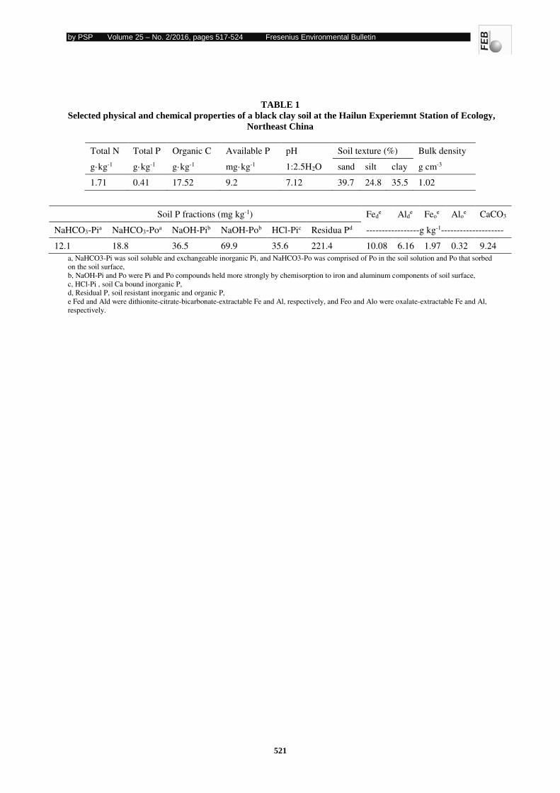
by PSP Volume 25 – No. 2/2016, pages 517-524 Fresenius Environmental Bulletin
521
TABLE 1
Selected physical and chemical properties of a black clay soil at the Hailun Experiemnt Station of Ecology,
Northeast China
Total N Total P Organic C Available P pH Soil texture (%) Bulk density
g·kg-1 g·kg-1 g·kg-1 mg·kg-1 1:2.5H2O sand silt clay g cm-3
1.71 0.41 17.52 9.2 7.12 39.7 24.8 35.5 1.02
Soil P fractions (mg kg-1) Fede Ald
e Feoe Alo
e CaCO3
NaHCO3-Pia NaHCO3-Poa NaOH-Pib NaOH-Pob HCl-Pic Residua Pd -----------------g kg-1--------------------
12.1 18.8 36.5 69.9 35.6 221.4 10.08 6.16 1.97 0.32 9.24
a, NaHCO3-Pi was soil soluble and exchangeable inorganic Pi, and NaHCO3-Po was comprised of Po in the soil solution and Po that sorbed
on the soil surface,
b, NaOH-Pi and Po were Pi and Po compounds held more strongly by chemisorption to iron and aluminum components of soil surface,
c, HCl-Pi , soil Ca bound inorganic P,
d, Residual P, soil resistant inorganic and organic P,
e Fed and Ald were dithionite-citrate-bicarbonate-extractable Fe and Al, respectively, and Feo and Alo were oxalate-extractable Fe and Al,
respectively.
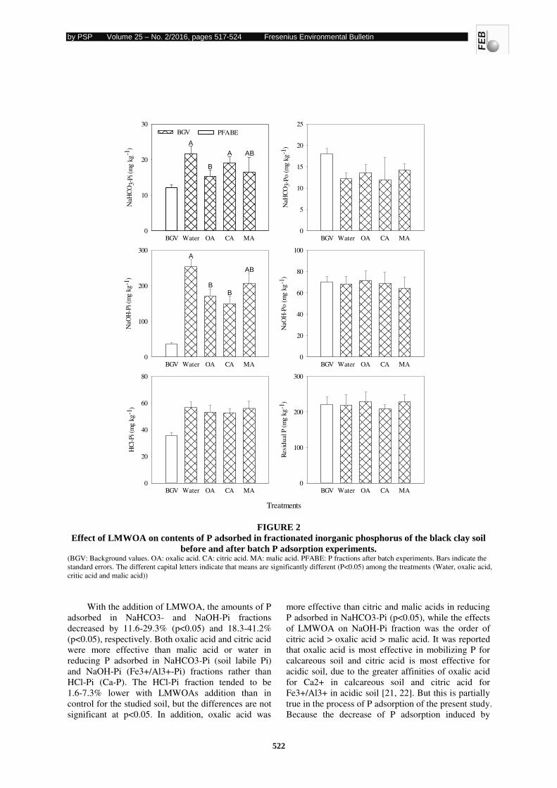
by PSP Volume 25 – No. 2/2016, pages 517-524 Fresenius Environmental Bulletin
522
BGV Water OA CA MA
NaH
CO
3-P
i (m
g k
g-1
)
0
10
20
30
BGV PFABE
BGV Water OA CA MA
NaH
CO
3-P
o (
mg
kg
-1)
0
5
10
15
20
25
BGV Water OA CA MA
NaO
H-P
i (m
g k
g-1
)
0
100
200
300
BGV Water OA CA MA
NaO
H-P
o (
mg
kg
-1)
0
20
40
60
80
100
BGV Water OA CA MA
HC
l-P
i (m
g k
g-1
)
0
20
40
60
80
Treatments
BGV Water OA CA MA
Res
idu
al P
(m
g k
g-1
)
0
100
200
300
A
A
B
AB
A
AB
BB
FIGURE 2
Effect of LMWOA on contents of P adsorbed in fractionated inorganic phosphorus of the black clay soil
before and after batch P adsorption experiments. (BGV: Background values. OA: oxalic acid. CA: citric acid. MA: malic acid. PFABE: P fractions after batch experiments. Bars indicate the
standard errors. The different capital letters indicate that means are significantly different (P<0.05) among the treatments (Water, oxalic acid,
critic acid and malic acid))
With the addition of LMWOA, the amounts of P
adsorbed in NaHCO3- and NaOH-Pi fractions
decreased by 11.6-29.3% (p<0.05) and 18.3-41.2%
(p<0.05), respectively. Both oxalic acid and citric acid
were more effective than malic acid or water in
reducing P adsorbed in NaHCO3-Pi (soil labile Pi)
and NaOH-Pi (Fe3+/Al3+-Pi) fractions rather than
HCl-Pi (Ca-P). The HCl-Pi fraction tended to be
1.6-7.3% lower with LMWOAs addition than in
control for the studied soil, but the differences are not
significant at p<0.05. In addition, oxalic acid was
more effective than citric and malic acids in reducing
P adsorbed in NaHCO3-Pi (p<0.05), while the effects
of LMWOA on NaOH-Pi fraction was the order of
citric acid > oxalic acid > malic acid. It was reported
that oxalic acid is most effective in mobilizing P for
calcareous soil and citric acid is most effective for
acidic soil, due to the greater affinities of oxalic acid
for Ca2+ in calcareous soil and citric acid for
Fe3+/Al3+ in acidic soil [21, 22]. But this is partially
true in the process of P adsorption of the present study.
Because the decrease of P adsorption induced by
by PSP Volume 25 – No. 2/2016, pages 517-524 Fresenius Environmental Bulletin
523
oxalic acid was mainly due to the effect of oxalic acid
on the NaHCO3-Pi fraction, but not the displacement
of P from Ca-P complexes by oxalic acid ligands.
These results showed that the decrease of P
adsorption induced by LMWOA was mainly ascribed
to the reduced P adsorbed in NaHCO3- and NaOH-Pi
fractions.
CONCLUSIONS
This work was designed to study the
mechanisms of P adsorption perturbed by LMWOA
using the batch experiments followed by sequential P
fractionation in a black clay soils. Results revealed
that LMWOA (oxalic acid, citric acid and malic acid)
reduced P adsorption by soils through decreasing the
amounts of P adsorbed in NaHCO3-Pi (soil labile Pi)
and NaOH-Pi (Fe/Al-Pi) fractions. Further studies on
speciation analysis of P by means of 31P-NMR and
XANES in P adsorption processes involved in
LMWOAs are warranted.
ACKNOWLEDGEMENTS
This work is financially supported by Science
Research and Technology Development Program of
Guangxi (Grant No. 2014DD29090).
REFERENCES
[1] Chen, C.R., Condron, L.M. and Xu, Z.H. (2008)
Impacts of grassland afforestation with
coniferous trees on soil phosphorus dynamics
and associated microbial processes: A review.
Forest Ecol. Manag, 255(3-4), 396-409.
[2] Palomo, L., Claassenb, N. and Jones, D.L. (2006)
Differential mobilization of P in the maize
rhizosphere by citric acid and potassium citrate.
Soil Biol. Biochem, 38(4), 683-692.
[3] Harrold, S.A. and Tabatabai, M.A. (2006)
Release of inorganic phosphorus from soils by
low-molecular-weight organic acids. Commun.
Soil Sci. Plan, 37(9-10), 1233-1245.
[4] Nwoke, O.C., Diels, J., Abaidoo, R., Nziguheba,
G. and Merckx, R. (2008) Organic acids in the
rhizosphere and root characteristics of soybean
(Glycine max) and cowpea (Vigna unguiculata)
in relation to phosphorus uptake in poor savanna
soils. African J. Biotech, 7(20), 3617-3624.
[5] Taghipour, M. and Jalali, M. (2013) Effect of
low-molecular-weight organic acids on kinetics
release and fractionation of phosphorus in some
calcareous soils of western Iran. Environ Monit
Asses 185(7), 5471-5482.
[6] Zhang, W., Niu, J., Ming, Q., Chen, G., Shi, Z.
and Long, X. (2015) Spatial-temporal variations
of phosphorus and ammonia nitrogen of
Baoxiang River, dianchi lake catchment.
Fresenius Environ. Bull, 24(8A), 2673-2681.
[7] Wang, H., Bo, G. and Liu, X. (2015) Chemical
reaction kinetics analysis of removing
phosphorus pollutants from wastewater in
different constructed wetlands. Fresenius
Environ. Bull, 24(2A), 596-601.
[8] Zheng, X., Wei, Y., Chen, Y., Wan, R., Tang, S.,
Su, Y. and Wu, L. (2015) Mitigation of adverse
effects of zinc oxide nanoparticles on enhanced
biological phosphorus removal: role of carbon
source concentration. Fresenius Environ. Bull,
24(5), 1699-1706.
[9] Del Bubba, M., Arias, C.A. and Brix, H. (2003)
Phosphorus adsorption maximum of sands for
use as media in subsurface flow constructed reed
beds as measured by the Langmuir isotherm.
Water Res, 37(14), 3390-3400.
[10] Jones, D.L. (1998) Organic acids in the
rhizosphere - a critical review. Plant Soil, 205(1),
25-44.
[11] Wei, L.L., Chen, C.R. and Xu, Z.H. (2010)
Citric acid enhances the mobilization of organic
phosphorus in subtropical and tropical forest
soils. Biol. Fert. Soils, 46(7), 765-769.
[12] Olsen, S.R., Cole, C., Watanabe, F.S. and Dean,
L. (1954) Estimation of available phosphorus in
soils by extraction with sodium bicarbonate, 939.
USDA Washington, DC.
[13] Hedley, M., Stewart, J. and Chauhan, B. (1982)
Changes in inorganic and organic soil
phosphorus fractions induced by cultivation
practices and by laboratory incubations. Soil Sci.
Soc. Am. J, 46(5), 970-976.
[14] Kang, J., Amoozegar, A., Hesterberg, D. and
Osmond, D.L. (2011) Phosphorus leaching in a
sandy soil as affected by organic and inorganic
fertilizer sources. Geoderma, 161(3-4), 194-201.
[15] Börling, K., Otabbong, E. and Barberis, E. (2001)
Phosphorus sorption in relation to soil properties
in some cultivated Swedish soils. Nutr. Cycl.
Agroecosys, 59(1), 39-46.
[16] Bus, A.Z., Karczmarczyk, A. (2015) Kinetic and
sorption equilibrium studies on phosphorus
removal from natural swimming ponds by
selected reactive materials. Fresenius Environ.
Bull, 24(9), 2736-2741.
[17] Ström, L., Owen, A.G., Godbold, D.L. and Jones,
D.L. (2005) Organic acid behaviour in a
calcareous soil implications for rhizosphere
nutrient cycling. Soil Biol. Biochem, 37(11),
2046-2054.
[18] Wang, C., Wang, Z., Lin, L., Tian, B. and Pei, Y.
(2012) Effect of low molecular weight organic
by PSP Volume 25 – No. 2/2016, pages 517-524 Fresenius Environmental Bulletin
524
acids on phosphorus adsorption by ferric-alum
water treatment residuals. J. Hazard. Mater,
203-204, 145-150.
[19] Bais, H.P., Weir, T.L., Perry, L.G., Gilroy, S.
and Vivanco, J.M. (2006) The role of root
exudates in rhizosphere interations with plants
and other organisms. Annu. Rev. Plant Biol, 57,
233-266.
[20] Moradi, N., Sadaghiani, M.H.R., Sepehr, E. and
Mandoulakani, B.A. (2012) Effects of
low-molecular-weight organic acids on
phosphorus sorption characteristics in some
calcareous soils. Turkish J. Agri. Forest, 36(4),
459-468.
[21] Hayes, J.E., Richardson, A.E. and Simpson, R.J.
(2000) Components of organic phosphorus in
soil extracts that are hydrolysed by phytase and
acid phosphatase. Biol. Fert. Soils, 32(4),
279-286.
[22] Strom, L., Owen, A.G., Godbold, D.L. and Jones,
D.L. (2001) Organic acid behaviour in a
calcareous soil: sorption reactions and
biodegradation rates. Soil Biol. Biochem, 33(15),
2125-2133.
Received: 09.07.2015
Accepted: 17.01.2016
CORRESPONDING AUTHOR
Yan Yan
Guangxi Teachers Education University
Nanning 530001 – P.R. CHINA
e-mail: [email protected] (Yan Yan),
[email protected] (Yongzhuang Wang)
by PSP Volume 25 – No. 2/2016, pages 525-533 Fresenius Environmental Bulletin
525
CONTAMINATION STATUS OF ERZENI RIVER, ALBANIA
DUE TO HEAVY METALS SPATIAL AND TEMPORAL
DISTRIBUTION
Alma Shehu1, MajlindaVasjari1, Edlira Baraj2, Rajmonda Lilo2, Roza Allabashi3
1Department of Chemistry, Faculty of Natural Sciences, University of Tirana
2Departmentof Chemistry, Faculty of Mathematical Engineering and Physical Engineering, Polytechnic University of Tirana 3University of Natural Resources and Life Sciences, Vienna; Department of Water, Atmosphere and Environment, Institute of Sanitary
Engineering and Water Pollution Control
ABSTRACT
Heavy metals are considered as serious
pollutants of aquatic ecosystems because of their
environmental persistence, toxic potential and
ability to be incorporated into the food chain. In the
present investigation, the contamination status of
one section of Erzeni River was assessed in regard
to occurrence and distribution of some heavy
metals. Due to concerns about potential pollution
resulting from watershed sources and adjacent
increased human activities, the study was
performed at a representative section of this river,
during the period December 2013-April 2014. The
filterable fraction of heavy metals such as Pb, Cu,
Cd, Zn and Ni was determined using the GF-AAS
technique. BGBI.II, Nr. 96/2006 as well as
2008/105/EC Directives were used for the
estimation of the contamination status of the river
water. Distribution of heavy metals in the river
water was also evaluated by means of the
Contamination Index (CI) and the Mean
Contamination Index (MCI), values. The relative
abundance of heavy metals followed the order:
Zn>Ni>Pb>Cu>Cd, while probability plots ( =
0.05) confirm that external pressures can contribute
to heavy metal levels in waters of Erzeni River.
Although CI varied evidently in different sites,
assuming that the levels of heavy metals are very
dependent with location, the MCI values prove that
there exist a high degree of spatial and temporal
homogeneity at all scales due to a high rate of water
mixing in the river.
KEYWORDS: Heavy Metals, Water Contamination, Erzeni River.
INTRODUCTION
The fate of heavy metals introduced by human
activities, chemical and geochemical processes into
the aquatic ecosystem have recently become subject
of widespread concern; since beyond the tolerable
limits they may become very toxic [1]. Sediments
and biota are generally metal reservoirs in aquatic
environment and may assume several orders of
magnitude greater than the amount found in water
[2]. Contamination of surface water systems by
heavy metals may be either due to natural or
anthropogenic activities. Naturally occurring metals
move through aquatic environments independently
of human activities, usually without any detrimental
effects [3, 4]. Some of these metals are essential for
proper metabolism in all living organisms yet toxic
at high concentrations; other metals currently
thought of as non-essential are toxic even at
relatively low concentrations [5]. Major sources of
toxic metals arising from human activities are
domestic and industrial wastewaters and their
associated solid wastes. Metal contamination can
also originate from industrial activities as well as
from urban storm water runoff from roads, parking
areas and other impervious surfaces, ending up
either in waste water treatment plants, or directly in
the river [6].
Metals that are naturally introduced into the
river come primarily from such sources as rock
weathering, soil erosion, or the dissolution of
water-soluble salts [7]. All heavy metals exist in
surface waters in colloidal, particulate and
dissolved phases, although dissolved concentrations
are generally low. The solubility of trace metals in
surface waters is predominately controlled by the
water pH, the type and concentration of ligands on
which the metal could adsorb and the redox
environment of the system [8, 9].
Albania is rich in water resources, including
rivers, groundwater, lakes, lagoons and seas.
Although its resources exceed by far its
consumption, locally water shortage and conflicts
among users may occur in the dry season [10].
General assessment of the state of HM
pollution of rivers is difficult, primarily because
measurements of metals are rarely included in
by PSP Volume 25 – No. 2/2016, pages 525-533 Fresenius Environmental Bulletin
526
monitoring programmes, but also because
concentration levels are usually so low that
problems arise with sample preparation and the
precision of analytical results [11, 12]. Comparison
and assessment of the state of HM in rivers is
therefore more difficult than for most of the other
water quality variables.
Erzeni River is located in the western part of
Albania. It springs from the east mountains of
Tirana city, near the Shëngjergji village and flows
west through Bërzhitë, Petrelë, Vaqarr, Ndroq,
Shijak and Sukth into the Adriatic Sea, north of
Durrësi [10]. The catchment of this river is about
759 km2 while its annual discharge volume is about
1,439 million m3, with a specific discharge of about
31 L/sec*km2. The water quality is poor as the river
flows through one of the most developed urban
areas of the central part of Albania. In recent years,
human activities such as abusive deforestation, the
plugging up of new agricultural lands and their
intensive cultivation, extraction of gravel and sand
from the riverbed have been intensified [10].
Environmental situation of the main rivers in
Albania has been monitored in the framework of
several national and international projects [12, 13,
14]. Previous studies on Erzeni River have been
focused mainly on physical-chemical parameters
while there are no reliable studies regarding heavy
metals. The aim of the present study was the
evaluation of the spatial and temporal
contamination of this section of Erzeni River due to
heavy metals levels in the water.
Evaluation of the contamination status of
waters of Erzeni River was carried out based on
two important standards, which determine the
allowable levels of heavy metals in surface waters,
such as BGBl.II, Nr. 96/2006,
“Qualitätszielverordnung Chemie Oberflächengewässer” and the 2008/105/EC Directive [15, 16].
MATERIAL AND METHODS
Estimation of the environmental situation of
Erzeni River regarding heavy metals content in
water was accomplished by determining the metals
content in water samples of four sites, selected in a
representative section of the river. The study was
performed in different months, during the period
December 2013-April 2014.
Sampling procedure for water samples.
Water samples were manually collected at surface
depth in each site using PET bottles, according to
the standard method Nr 105, described in the
“Standard Methods for the Examination of Water
and Waste Water”, case of heavy metals [17]. Samples were transported to the laboratory within
the same day, using cooling boxes, were
immediately filtered with 0.45µm glass filters and
the filtrate was acidified to pH=2 with concentrated
HNO3.
Acidified samples were stored at temperature
+4oC till the analyses. The analyzed metals were
Copper, Cadmium, Lead, Nickel, Zinc and their
content in water samples was determined according
to the standard method Nr 304 of the “Standard Methods for the Examination of Water and Waste
Water” [17]. NOVAA 400 Atomic Absorption
Spectrometer, equipped with a graphite furnace
system, was used to carry out water analyses.
Analytical blanks were run in the same way as
the samples and concentration was determined
using standard solutions prepared in the same acid
matrix. Results are expressed in μg.L-1, as well as
standard deviation was calculated for three repeated
analyses of each sample
Sampling sites description. The water quality
of Erzeni River was monitored in four selected sites
along the river, namely S1- located at Ibe area; S2-
located at Peshkatari Bridge ; S3- located at Domje
Bridge; S4- located at Sharra area. The sampling site S1 is located in the
upstream area of the river, being suggested as the
reference point. At the area of S2, a considerable
number of restaurants and hotels develop their
activities, while in S3 extraction of gravels is
evident in several points. Station S4 is located close
to the Sharra landfill, classified by the UNEP, 2000,
as a “hot spot” area in Albania [18]. Before the landfill construction, Sharra dump was the most
potential source of pollutants of Erzeni River, for
both inorganic and organic pollutants [19].
Location of all selected sampling sites for the
present study is illustrated in figure 1.
Quality control of measurements and statistical analysis. Quality control of the results
was conducted by analyzing a certified reference
material (QC-TM#1), provided by GEMS/Water
(PE) Study No 8, 2013. Obtained results were in
good agreement with the certified values given in
respective certificates of the CRM (z-score ranging
between -0.03 to-0.6). The concentration of each
metal in water samples in Erzeni River was
calculated using linear regression and expressed in
µg.L-1 as the mean value of three sample replicates.
Limit of quantification (LOQ) and working range
for each element studied in this work are presented
in table 1. Descriptive statistics including mean, standard
deviation, min, max, value and median were
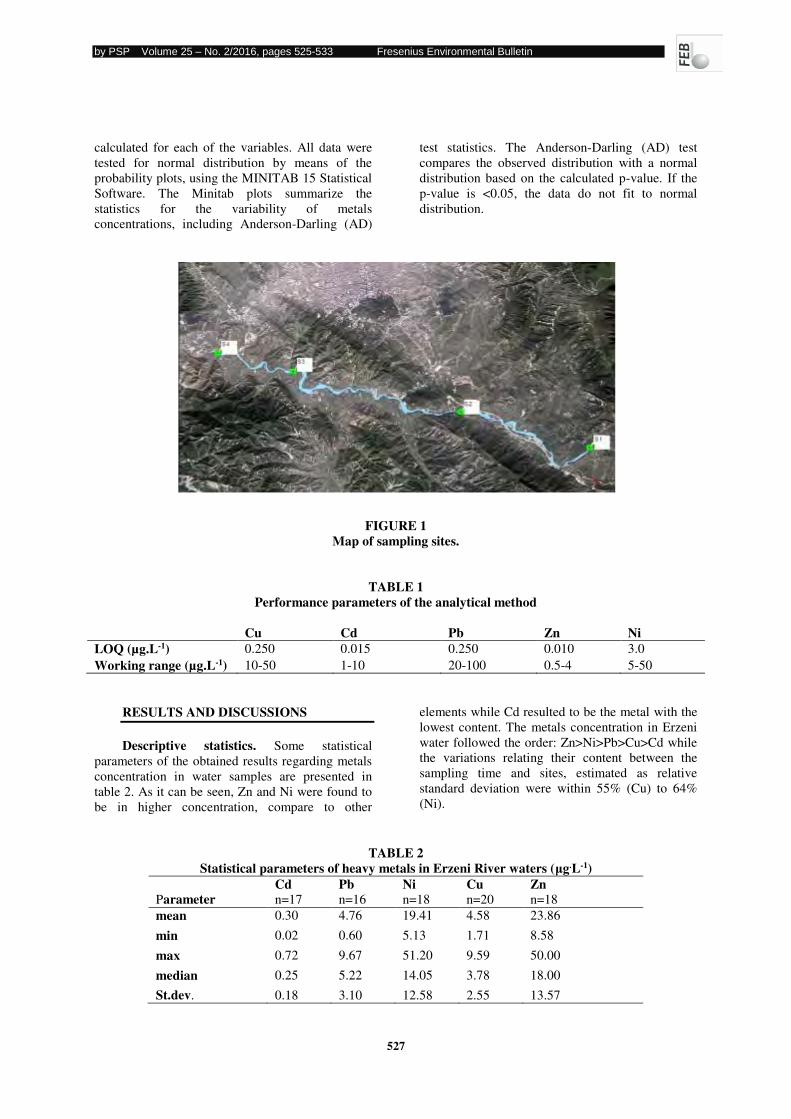
by PSP Volume 25 – No. 2/2016, pages 525-533 Fresenius Environmental Bulletin
527
calculated for each of the variables. All data were
tested for normal distribution by means of the
probability plots, using the MINITAB 15 Statistical
Software. The Minitab plots summarize the
statistics for the variability of metals
concentrations, including Anderson-Darling (AD)
test statistics. The Anderson-Darling (AD) test
compares the observed distribution with a normal
distribution based on the calculated p-value. If the
p-value is <0.05, the data do not fit to normal
distribution.
FIGURE 1 Map of sampling sites.
TABLE 1 Performance parameters of the analytical method
Cu Cd Pb Zn Ni LOQ (µg.L-1) 0.250 0.015 0.250 0.010 3.0
Working range (µg.L-1) 10-50 1-10 20-100 0.5-4 5-50
RESULTS AND DISCUSSIONS
Descriptive statistics. Some statistical
parameters of the obtained results regarding metals
concentration in water samples are presented in
table 2. As it can be seen, Zn and Ni were found to
be in higher concentration, compare to other
elements while Cd resulted to be the metal with the
lowest content. The metals concentration in Erzeni
water followed the order: Zn>Ni>Pb>Cu>Cd while
the variations relating their content between the
sampling time and sites, estimated as relative
standard deviation were within 55% (Cu) to 64%
(Ni).
TABLE 2 Statistical parameters of heavy metals in Erzeni River waters (μg.L-1)
Parameter
Cd n=17
Pb n=16
Ni n=18
Cu n=20
Zn n=18
mean 0.30 4.76 19.41 4.58 23.86
min 0.02 0.60 5.13 1.71 8.58
max 0.72 9.67 51.20 9.59 50.00
median 0.25 5.22 14.05 3.78 18.00
St.dev. 0.18 3.10 12.58 2.55 13.57
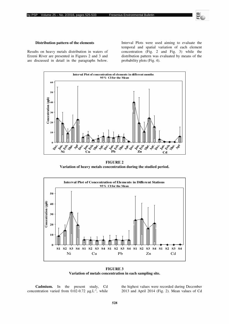
by PSP Volume 25 – No. 2/2016, pages 525-533 Fresenius Environmental Bulletin
528
Distribution pattern of the elements
Results on heavy metals distribution in waters of
Erzeni River are presented in Figures 2 and 3 and
are discussed in detail in the paragraphs below.
Interval Plots were used aiming to evaluate the
temporal and spatial variation of each element
concentration (Fig. 2 and Fig. 3) while the
distribution pattern was evaluated by means of the
probability plots (Fig. 4).
Apr
Mar
.
Feb.
Jan.
Dec
.
Apr
.
Mar
.
Feb.
Jan.
Dec
.
Apr
.
Mar
.
Feb.
Jan.
Dec
.
Apr
.
Mar
.
Feb.
Jan.
Dec
.
Apr
Mar
.
Feb.
Jan.
Dec
.
60
50
40
30
20
10
0
Con
cent
rati
on (
ppb)
95% CI for the MeanInterval Plot of concentration of elements in different months
Ni Cu Pb Zn Cd
FIGURE 2 Variation of heavy metals concentration during the studied period.
S4S3S2S1S4S3S2S1S4S3S2S1S4S3S2S1S4S3S2S1
50
40
30
20
10
0
Con
cent
rati
on (
ppb)
95% CI for the MeanInterval Plot of Concentration of Elements in Different Stations
Ni Cu Pb Zn Cd
FIGURE 3 Variation of metals concentration in each sampling site.
Cadmium. In the present study, Cd
concentration varied from 0.02-0.72 μg.L-1, while
the highest values were recorded during December
2013 and April 2014 (Fig. 2). Mean values of Cd
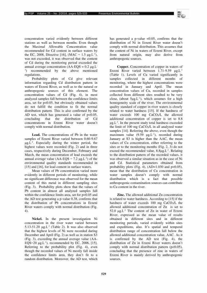
by PSP Volume 25 – No. 2/2016, pages 525-533 Fresenius Environmental Bulletin
529
concentration varied evidently between different
stations as well as between months. Even though
the Maximal Allowable Concentration value
recommended for Cd content in surface waters by
the EC, 2008, Directive [16], (MAC = 1.5 μg.L-1),
was not exceeded, it was observed that the content
of Cd during the monitoring period exceeded the
annual average concentration (AA-EQS = 0.2 μg.L-
1) recommended by the above mentioned
regulations.
Probability plots of Cd give relevant
information regarding Cd distribution pattern in
waters of Erzeni River, as well as to the natural or
anthropogenic sources of this element. The
concentration values of Cd (Fig. 4), in most
analyzed samples fall between the confidence limits
area, set for p<0.05, but obviously obtained values
do not fulfill the condition to fit the normal
distribution pattern. This is also confirmed by the
AD test, which has generated a value of p<0.05,
concluding that the distribution of Cd
concentrations in Erzeni River water doesn’t comply with normal distribution.
Lead. The concentrations of Pb in the water
samples of Erzeni River varied between 0.60-9.67
μg.L-1. Especially during the winter period, the
highest values were recorded (Fig. 2) and in three
cases, respectively during December, February and
March, the mean concentration of lead exceeds the
annual average value (AA-EQS = 7.2 μg.L-1) of the
environmental quality standards recommended in
[15] and [16], for lead content in surface waters. Mean values of Pb concentration varied more
evidently in different periods of monitoring, while
no significant difference was observed for the mean
content of this metal in different sampling sites
(Fig. 3). Probability plots show that the values of
Pb content in almost all analyzed samples fall
within the confidence limits area, set for p<0.05 and
the AD test generating a p-value 0.38, confirms that
the distribution of Pb concentrations in Erzeni
River waters comply with normal distribution (Fig.
4).
Nickel. In the present investigation Ni
concentration in the river water varied between
5.13-51.20 μg.L-1 (Table 2). It was also observed
that the highest levels of Ni were recorded during
December and April (Fig. 2) as well as in station S3
(Fig. 3), exceeding the annual average value (AA-
EQS=20 μg.L-1), recommended by EC, 2006, [15].
Referring to the probability plot (Fig. 4), even
though the recorded values of Ni mostly fall inside
the confidence limits area, they don’t fit to a random distribution. Moreover, the AD test, which
has generated a p-value <0.05, confirms that the
distribution of Ni in Erzeni River water doesn’t comply with normal distribution. This assumes that
the content of Ni in waters of Erzeni River, except
from natural origin, may also derive from
anthropogenic sources.
Copper. Concentration of copper in waters of
Erzeni River varied between 1.71-9.59 μg.L-1
(Table 1). Levels of Cu varied significantly in
samples collected in different months of
monitoring, where the highest concentrations were
recorded in January and April. The mean
concentration values of Cu, recorded in samples
collected from different sites resulted to be very
close, (about 5μg.L-1), which assumes for a high
homogeneity scale of the river. The environmental
quality standard of copper in river waters is closely
related to water hardness [15]. If the hardness of
water exceeds 100 mg CaCO3/L the allowed
additional concentration of copper is set to 8.8
μg.L-1. In the present study total hardness exceeded
the limit of 100 mg CaCO3/L in all analyzed water
samples [14]. Referring the above, even though the
maximum value (9.59 μg.L-1), recorded during
January at S3 is higher than the AAC, the mean
values of Cu concentration, either referring to the
sites or to the monitoring months (Fig. 2, 3) do not
exceed the recommended value, 8.8μg.L-1. Relating
to the distribution pattern of the recorded values, it
was observed a similar situation as in the case of Ni
and Cd. Statistical parameters obtained from
probability plots (Fig. 4), (AD=1.030 and p<0.05),
mean that the distribution of Cu concentration in
water samples doesn’t comply with normal distribution which is a fact that possible
anthropogenic contamination sources can contribute
to Cu content in the river.
Zinc. The allowed additional Zn concentration
is related to water hardness. According to [15] if the
hardness of water exceeds 100 mg CaCO3/L the
allowed additional concentration of Zn is set to
52.0 μg.L-1 The content of Zn in water of Erzeni
River, expressed as the mean value of results
obtained in different sites and in different
monitoring periods, varied evidently within sites
and expeditions, also. It’s spatial and temporal distribution range of concentration fall below the
allowed additional concentration value, AAC. As it
is confirmed by the AD test (Fig. 4), the
distribution of Zn in Erzeni River waters doesn’t comply with normal distribution pattern (p<0.05),
concluding that the presence of zinc in waters of
Erzeni River is mainly derived by anthropogenic
sources.
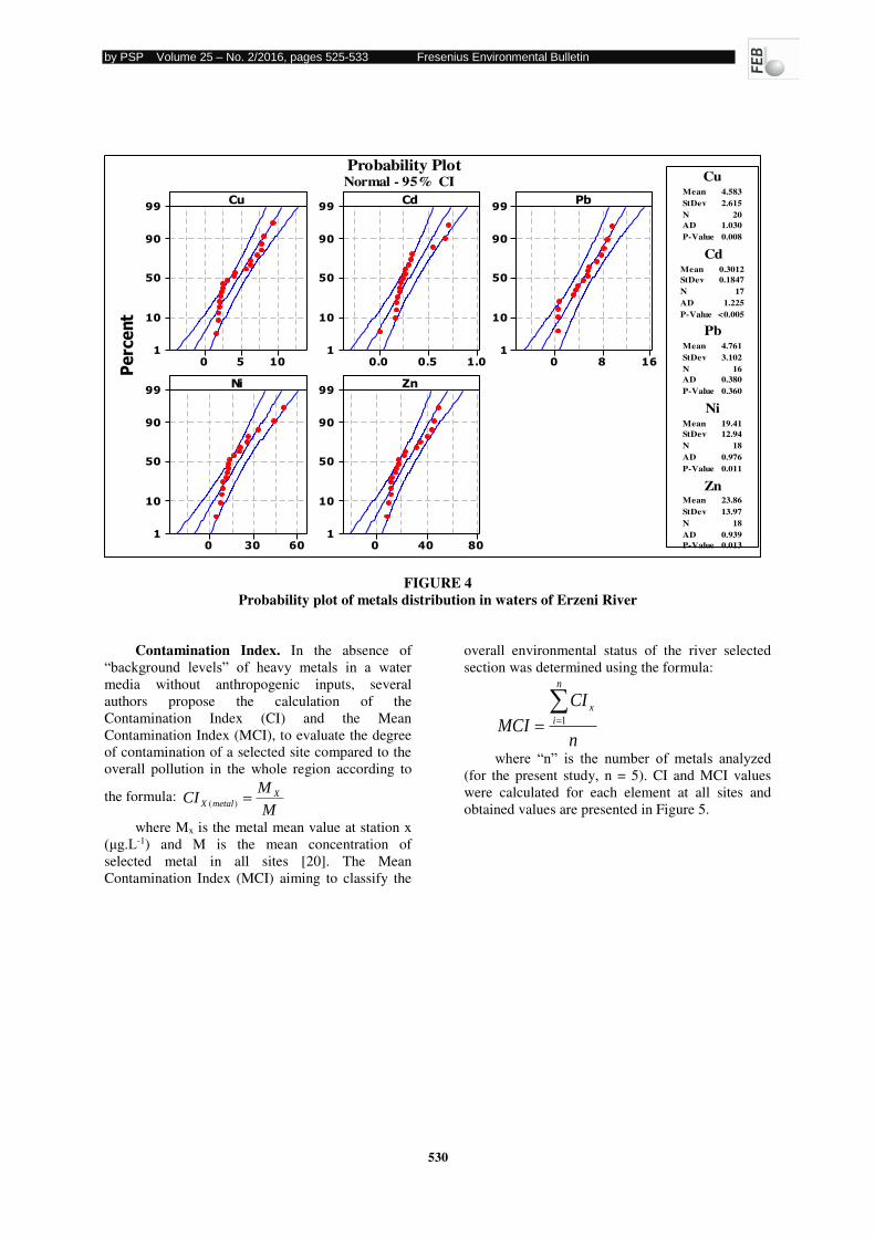
by PSP Volume 25 – No. 2/2016, pages 525-533 Fresenius Environmental Bulletin
530
1050
99
90
50
10
1
1.00.50.0
99
90
50
10
1
1680
99
90
50
10
1
60300
99
90
50
10
1
80400
99
90
50
10
1
Cu
Percent
Cd Pb
Ni Zn
Mean 4.583
StDev 2.615
N 20AD 1.030
P-Value 0.008
Cu
Mean 0.3012StDev 0.1847
N 17
AD 1.225
P-Value <0.005
Cd
Mean 4.761
StDev 3.102
N 16AD 0.380
P-Value 0.360
Pb
Mean 19.41StDev 12.94
N 18
AD 0.976
P-Value 0.011
Ni
Mean 23.86
StDev 13.97
N 18
AD 0.939P-Value 0.013
Zn
Normal - 95% CIProbability Plot
FIGURE 4 Probability plot of metals distribution in waters of Erzeni River
Contamination Index. In the absence of
“background levels” of heavy metals in a water media without anthropogenic inputs, several
authors propose the calculation of the
Contamination Index (CI) and the Mean
Contamination Index (MCI), to evaluate the degree
of contamination of a selected site compared to the
overall pollution in the whole region according to
the formula:
M
MCI
X
metalX)(
where Mx is the metal mean value at station x
(μg.L-1) and M is the mean concentration of
selected metal in all sites [20]. The Mean
Contamination Index (MCI) aiming to classify the
overall environmental status of the river selected
section was determined using the formula:
n
CI
MCI
n
i
x 1
where “n” is the number of metals analyzed
(for the present study, n = 5). CI and MCI values
were calculated for each element at all sites and
obtained values are presented in Figure 5.
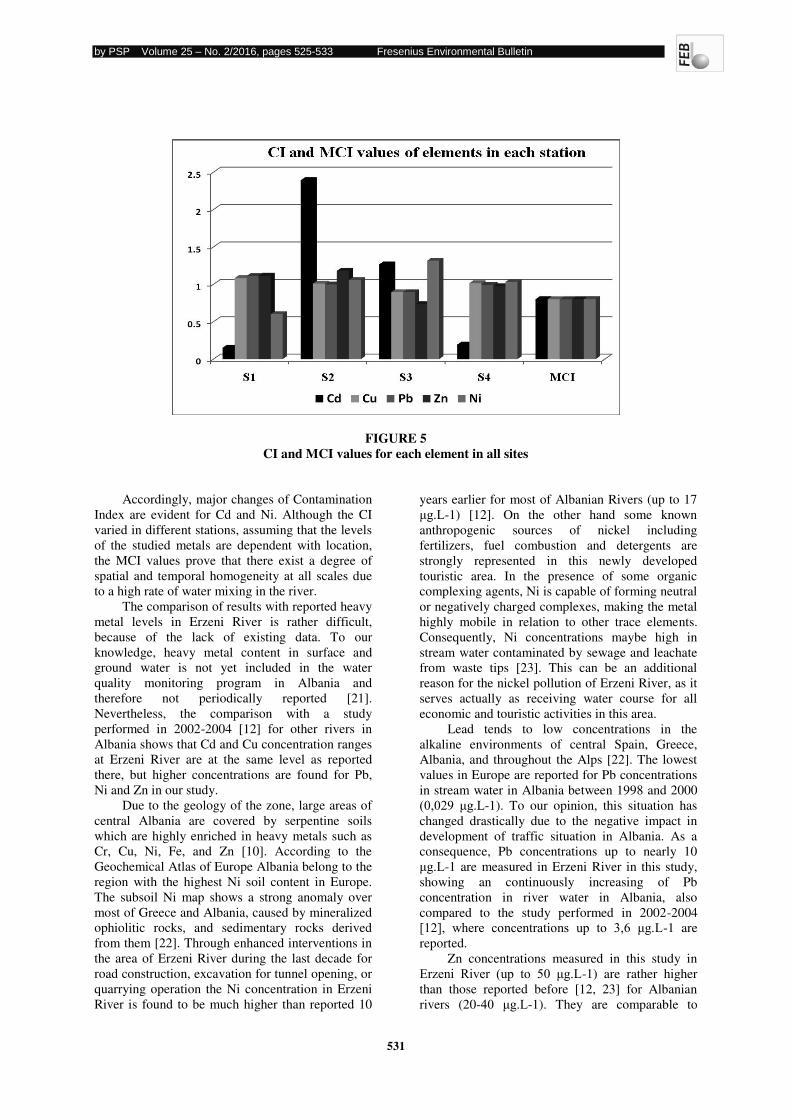
by PSP Volume 25 – No. 2/2016, pages 525-533 Fresenius Environmental Bulletin
531
FIGURE 5 CI and MCI values for each element in all sites
Accordingly, major changes of Contamination
Index are evident for Cd and Ni. Although the CI
varied in different stations, assuming that the levels
of the studied metals are dependent with location,
the MCI values prove that there exist a degree of
spatial and temporal homogeneity at all scales due
to a high rate of water mixing in the river.
The comparison of results with reported heavy
metal levels in Erzeni River is rather difficult,
because of the lack of existing data. To our
knowledge, heavy metal content in surface and
ground water is not yet included in the water
quality monitoring program in Albania and
therefore not periodically reported [21].
Nevertheless, the comparison with a study
performed in 2002-2004 [12] for other rivers in
Albania shows that Cd and Cu concentration ranges
at Erzeni River are at the same level as reported
there, but higher concentrations are found for Pb,
Ni and Zn in our study.
Due to the geology of the zone, large areas of
central Albania are covered by serpentine soils
which are highly enriched in heavy metals such as
Cr, Cu, Ni, Fe, and Zn [10]. According to the
Geochemical Atlas of Europe Albania belong to the
region with the highest Ni soil content in Europe.
The subsoil Ni map shows a strong anomaly over
most of Greece and Albania, caused by mineralized
ophiolitic rocks, and sedimentary rocks derived
from them [22]. Through enhanced interventions in
the area of Erzeni River during the last decade for
road construction, excavation for tunnel opening, or
quarrying operation the Ni concentration in Erzeni
River is found to be much higher than reported 10
years earlier for most of Albanian Rivers (up to 17
μg.L-1) [12]. On the other hand some known
anthropogenic sources of nickel including
fertilizers, fuel combustion and detergents are
strongly represented in this newly developed
touristic area. In the presence of some organic
complexing agents, Ni is capable of forming neutral
or negatively charged complexes, making the metal
highly mobile in relation to other trace elements.
Consequently, Ni concentrations maybe high in
stream water contaminated by sewage and leachate
from waste tips [23]. This can be an additional
reason for the nickel pollution of Erzeni River, as it
serves actually as receiving water course for all
economic and touristic activities in this area.
Lead tends to low concentrations in the
alkaline environments of central Spain, Greece,
Albania, and throughout the Alps [22]. The lowest
values in Europe are reported for Pb concentrations
in stream water in Albania between 1998 and 2000
(0,029 μg.L-1). To our opinion, this situation has
changed drastically due to the negative impact in
development of traffic situation in Albania. As a
consequence, Pb concentrations up to nearly 10
μg.L-1 are measured in Erzeni River in this study,
showing an continuously increasing of Pb
concentration in river water in Albania, also
compared to the study performed in 2002-2004
[12], where concentrations up to 3,6 μg.L-1 are
reported.
Zn concentrations measured in this study in
Erzeni River (up to 50 μg.L-1) are rather higher
than those reported before [12, 23] for Albanian
rivers (20-40 μg.L-1). They are comparable to
by PSP Volume 25 – No. 2/2016, pages 525-533 Fresenius Environmental Bulletin
532
typical concentrations in river water from the
literature, which are about 10-50 μg.L-1 [22]. These
high concentrations in stream water can be
explained with the high content of Zn in topsoil of
the region which is reported to be among the
highest in Europe [22]. The enhanced interventions
in the area of Erzeni River during the last decade,
especially excavations or quarrying operations can
be one of the reasons for the change of water
quality regarding Zn content in Erzeni River.
CONCLUSION
In the present study, the contamination status
of Erzeni River was assessed in regard to
occurrence and distribution of Pb, Cu, Cd, Zn and
Ni in one section of the river, represented by four
selected sites. The concentrations of studied heavy
metals are determined in the filterable sample
fraction. The European Water Frame Directive
(2008/105/EC) and the respective Austrian
regulation for surface water (BGBI.II, Nr. 96/2006)
were used to classify the contamination status of the
river water.
Except Cd, the means concentrations of other
metals were found to be lower than the values
recommended in those standards while the
variations relating the sampling time and sites were
within 55% (Cu) to 64% (Ni). The metal contents
were found to be in the order: Zn> Ni> Pb>Cu> Cd.
Comparative studies with other publications on
river water quality based on heavy metals contents
confirm that Cd and Cu concentration ranges at
Erzeni River are at the same level as reported there,
but higher concentrations are found for Pb, Ni and
Zn in our study. The enhanced interventions in the
area of Erzeni River during the last decade for road
construction, excavation for tunnel opening, or
quarrying operation have caused the enrichment of
water samples of Erzeni River with heavy metals
originated from the geology of the zone. On the
other hand, some known anthropogenic sources
including fertilizers, fuel combustion and detergents
are strongly represented in this newly developed
touristic area.Although the CI values varied
significantly for some elements such as Cd and Ni,
assuming that the levels of studied metals are
dependent with location, the MCI values prove that
there exist a degree of spatial and temporal
homogeneity at all scales due to a high rate of water
mixing in the river.
REFERENCES
[1] Manahan S. E., 2001. "Front matter
"Fundamentals of Environmental Chemistry.
Boca Raton: CRC Press LLC.
[2] Zhang Z., Wang J., Delaune R., 2015. Trace
elements contamination of Tangipahoa river
water and sediment in Louisiana. Fresenius
Environmental Bulletin, Vol. 24, No. 3, 910-
919.
[3] Qarri F., Kane S., Lazo P., 2014. Environmental
assessment of dissolved heavy metals in Vlora
Bay, Albania. Pranvera Lazo. Fresenius
Environmental Bulletin. Vol. 23 No. 7, 1539-
1546.
[4] Qi Y., Ma J., Fan G., 2015. Assessment of
heavy metals contamination in fen river
channels. Fresenius Environmental Bulletin.
Vol. 24, No. 5. 1230-1242.
[5] Baker, Lawrence A., Ed., 1994. Environmental
Chemistry of Lakes and Reservoirs, American
Chemical Society, Washington, D.C.
[6] Nicolau, R., Galera, C. A., and Lucas, Y., 2006.
Transfer of nutrients and labile metals from
the continent to the sea by a small
Mediterranean river, Chemosphere, 63 (3),
469 - 476.
[7] Hirsch, R.M., Hamilton, P.A., and Miller, T.L.,
2006. U.S. Geological Survey perspective on
water-quality monitoring and assessment.
Journal of Environmental Monitoring 8(5),
512-518.
[8] Forstner U, Wittmann G.T.W., 1981. Metal
Speciation in the Aquatic Environment, 2nd
ed., 26, Springer-Verlag.
[9] Huang Y., Zhang D., Li Y., Xu Zh., Yuan Sh.,
Wang L., 2015. Heavy metals sorption on
river sediments: kinetics, equilibria and
relative selectivities. Fresenius Environmental
Bulletin, Vol. 24, No. 09.
[10] Selenica A., Ardicioglu M.,Kuriqi A. Risk
assessment from floodings in the rivers of
Albania. International Balkans Conference on
Challenges of Civil Engineering, BCCCE, 19-
21 May 2011, EPOKA University, Tirana,
ALBANIA.
[11] Gashi F., Troni N., Hoti R., Faiku F., Ibrahimi
R., Laha F., Kurteshi K., Osmani S., Hoti F.,
2014. Chemical determination of some
elements in water of Sitnica river (Kosovo) by
ICP-MS technique. Fresenius Environmental
Bulletin, Vol. 23, No. 01.
[12] Miho A., Cullaj A., Hasko A., Lazo P., Kupe
L., Bachofen R., Brandl H., Schanz F., Baraj
B., 2005. “Environmental state of some rivers of Albanian Adriatic Lowland”, Evaluation
by PSP Volume 25 – No. 2/2016, pages 525-533 Fresenius Environmental Bulletin
533
Report/ Joint research project 7ALJ065583
(SCOPES).
[13] Flanagan M., Paukstys B., 2012, Report on:
“CEMSA Water Monitoring Field Survey and Training”.
[14] Project Report “Assessment of the water
quality of Erzeni River in Albania and the
impact of economic developments therein”, Ref. No. 1206.002A-13, co-financed by the
Central European Initiative (CEI) with
funding of the Austrian Development
Cooperation (ADC).
[15] BGBl.II, Nr. 96/2006,
“Qualitätszielverordnung Chemie Oberflächengewässer”.
[16] Directive 2008/105/EC of the European
Parliament and of the Council of 16 December
2008 on environmental quality standards in
the field of water policy.
[17] APHA, 1985. American Public Health
Association.Standard methods for the
examination of water and wastewater. 18th
Edition APHA Washington, DC.
[18] Post –conflict Environmental Assessment-
Albania UNEP 2000
[19] Billing K.,Wenborn M.,Selfo L., 2011.Sharra
Waste Dump Site, Albania-Feasibility Study
and Urgent Rehabilitation
Measures.http://www.sida.se/publications.
[20] Chafika, A., M.Cheggourb, D. Cossac and
Siffedine, S.B.M., 2001. Quality of Morocoan
Atlantic coastal waters: Water monitoring and
mussel watching. Aquatic Living Resour.,
14:239-249.
[21] State of the Environmental Report, Albania
2011, 2012, 2013, 2014
[22] Geological Atlas of Europe, Part1, ISBN 951-
690-913 2 (electronic version)
http://weppi.gtk.fi/publ/foregsatlas/index.php
[23] Cullaj A., Baraj B., 2007 “Assessment of the environmental situation of Albanian rivers
based on physico-chemical analyses”, http://siba-ese.unisalento.it/.
Received: 14.07.2015 Accepted: 10.12.2015
CORRESPONDING AUTHOR
Majlinda Vasjari
Department of Chemistry
Faculty of Natural Sciences
University of Tirana – ALBANIA
e-mail: [email protected]
by PSP Volume 25 – No. 2/2016, pages 534-547 Fresenius Environmental Bulletin
534
ANALYSIS ON REGIONAL CLIMATE AND
ATMOSPHERIC DROUGHT CHARACTERISTICS IN THE
NORTH SLOPE OF TIANSHAN MOUNTAIN IN XINJIANG,
CHINA
Aihong Fu1,2*, Yaning Chen1, Weihong Li1
1State key laboratory of desert and oasis ecology, Xinjiang Institute of Ecology and Geography, Chinese Academy of Sciences,
818 South Beijing Road, Urumqi, Xinjiang, China, 830011 2 Department of Biology, San Diego State University, San Diego, California, the United States,
5500 Campanile Drive, San Diego, CA 92182-4614
ABSTRACT
The drought as a universal natural
disaster not only can cause the agricultural
disaster, but also has a serious impact on
industrial production, urban water supply and
ecological environment. To explore whether
global warming could tend to increase
atmospheric drought in the north slope of
Tianshan Mountains in Xinjiang, China, we
collected the daily mean temperature,
precipitation, water vapor pressure and air
relative humidity of four typical counties
(Yining, Jinghe, Shihezi and Qitai counties) on
the north slope of Tianshan Mountains, and
analyzed the characteristics of temporal and
spatial variations of climatic factors and the
humid tendency of the north slope of Tianshan
Mountains. The results showed that 1)
temperature rose and precipitation increased in
all of the four in 1961-2013; 2) water vapor
pressure decreased in Yining county but
increased in other counties; and 3) air relative
humidity in Yining county and Shihezi
decreased, but unchanged in Jinghe and Qitai
counties. To relieve the drought tendency in
Yining County, it may be appropriate to reduce
the county's cultivated land area and return
farmland to forest and pasture land, which can
not only reduce crop production losses, but
also alleviate water shortage in the area.
KEYWORDS: Atmospheric drought; Climate change; The North
Slope of Tianshan Mountain; China
INTRODUCTION
Drought is a widely-distributed natural
disaster in the world, affecting more than 120
countries at different degrees. Only in China, it
affects 50% of the whole area subjected to
meteorological disasters. With the climate
warming, its outbreaks are characteristic of
high frequency, large distributed area, uneven
spatial and temporal distribution, and long
duration, etc. [1]. Drought impacts agricultural,
industrial, marine and other industry
productions, especially agricultural production
[2, 3]. High temperature can prolong the
growing season of crops and increase
evapotranspiration from farmland and
irrigation water demand [4, 5]. Fertilization
can lead to seasonal drought in crop fileds[6].
The changes in the drought pattern also bring
new challenges to water source management
[7]. Its resulted desertification of ecological
degradation and impacts on human society and
natural environment have attracted great and
widespread concerns all over the world [2].
To alleviate and prevent the
drought-induced adverse effects on the
environments, many researchers have
extensively explored the characteristics of
regional drought and established a series of
drought indicators to calculate and estimate the
severity of regional drought. These indicators
include meteorological indicators, soil
moisture index, crop physiological indicators,
corp water demand and supply indicators, the
percentage of model production targets, and
integrated crop moisture indicators. Some
scholars used different models to simulate and
predict the future drought of the
watershed[7,8-11], while others
comprehensively studied the spatial
distribution characteristics of drought
frequency from the aspects of climate,
vegetation and soil[12-15]. However, most of
them estimated the drought conditions from
the perspective of crop and soil water deficits,
very few studied the air temperature,
precipitation and air relative humidity from the
by PSP Volume 25 – No. 2/2016, pages 534-547 Fresenius Environmental Bulletin
535
point of view of atmospheric drought and by
means of atmospheric variation characteristics
to reflect the atmospheric, agricultural and
hydrological drought conditions. Previous
studies have indicated that atmospheric
drought is preceding the agricultural drought
and hydrological drought. When the
atmospheric evaporation capacity and
precipitation capability are at imbalance and
water usage is greater than the water supply,
the atmospheric humidity lowers and soil
moisture is deficit, crops will stop growing or
die due to lack of adequate water supply, and
river runoff is reduced due to excessive water
evaporation. Thus, understanding the
atmospheric drought conditions will help to
propose measures to alleviate atmospheric,
crops and hydrological droughts and provide
early warning for alleviating regional water
conflicts and water shortages, protecting
agricultural production and maintaining social
stability.
The north slope of Tianshan Mountains is
an important agricultural production base in
Xinjiang, China, and plays a very significant
role for Xinjiang's grain production, economic
development, and social stability. However in
recent decades, the ecological environment of
the north slope is worsening with the following
features: 1) Great recession of Tianshan glacier.
According to the 1981-2006 survey, the
thickness, area, volume, and snow line
decreased by 12.2%, 10.3%, 21.2% and 3.6%,
respectively[16]. From 1950s to 1970s, the
Ebinur Lake located in the north of Jinghe
County, Boertala Mongolian Autonomous
Prefecture, shrank at an annual average rate of
greater than 20 km2, 290 times as that of the
natural dry shrinkage period, from 1250 km2 in
1950s to 483 km2 in 2006[17]. Thus, it is clear
that the water source in the north slope of
Tianshan Mountains is gradually decreasing.
Over the past few decades, many scholars have
studied how climate of Tianshan Mountains
changes, whether its precipitation increases
and if so, whether it will positively affect river
runoff. They found that the temperature and
precipitation in Jinghe county (1953-2008),
Qitai county (1961-2002) and Shihezi
(1961-2010 years) all showed a upward trend.
In detail, the temperature of Jinghe county and
Qitai county obviously increased in winter
followed by fall; and precipitation in Jinghe
county, Shihezi County and Qitai county also
increased in the order of fall, summer and
winter [18-21]. However, Wang et al.[22]
found that increases in temperature and
precipitation did not significantly increase the
river runoff in the north slope of Tianshan
Mountains. Furthermore, Li et al.[23]found
that increase of the river runoff in the north
slope of Tianshan Mountains was the least in
the whole arid region of the northwest China
over the past 50 years. These results indicated
that the climate warming and increased
precipitation in Tianshan Mountains not only
did not increase water resource in the north
slope of Tainshan Mountains, it actually
accelerated the water resource shortage,
resulting in severe desertification process,
serious vegetation decline and reduced species
in the watershed[24].
Many scholars have tried to answer why
increased air temperature and precipitation in
the north slope of Tianshan Mountains
accelerated the water resource shortage,
whether climate changes could lead to drought
or humid status, and whether atmospheric
wetness could reflect the arid status and
explain the fact of no obvious water resource
increase in the north slope of Tianshan
Mountains. However, previous studies on the
temporal and spatial climate changes only
focused in Shihezi county before 2010 and did
not thoroughly explore the aridity in the
northern slope of Tianshan Mountains. In this
paper, we in-depth analyzed the varying
characteristics of air temperature, precipitation,
water vapor pressure, relative humidity and
other factors of the north slope of Tianshan
Mountains over the last 53 years, and based on
which, comprehensively determined the
wetness or drought status and explained the
reasons for arid situation in the basin and no
obvious water resource increase. We believe
that our research is extremely important not
only for understanding the current atmospheric
wetness status in the north slope of Tianshan
Mountains, but for providing atmospheric
drought mitigation measures and alleviating
regional water shortages and water use
conflicts, and maintaining the relatively
stability of natural and social ecosystems of
the northern slope of Tianshan Mountains.
MATERIALS AND METHODS
STUDY AREA
The north slope of Tianshan Mountains,
Xinjiang, China, mainly consists of the
northern regions of Bogda Mountain,
Yilianhabierga Mountain, and the watershed of
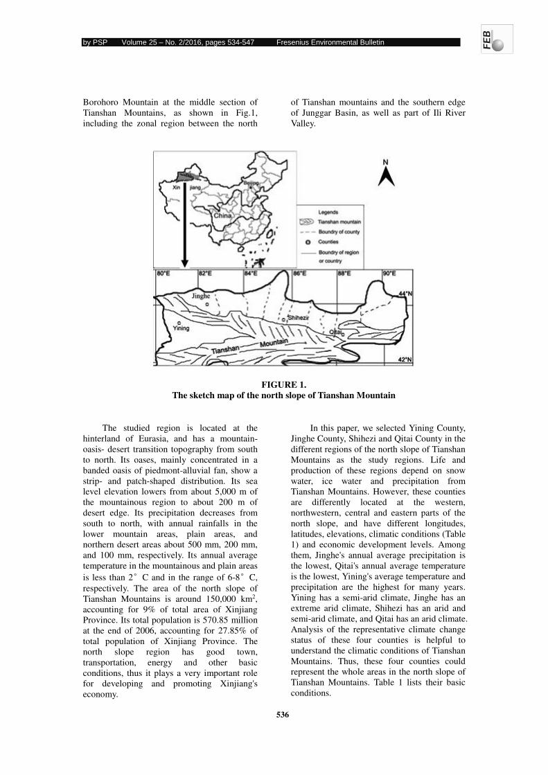
by PSP Volume 25 – No. 2/2016, pages 534-547 Fresenius Environmental Bulletin
536
Borohoro Mountain at the middle section of
Tianshan Mountains, as shown in Fig.1,
including the zonal region between the north
of Tianshan mountains and the southern edge
of Junggar Basin, as well as part of Ili River
Valley.
FIGURE 1.
The sketch map of the north slope of Tianshan Mountain
The studied region is located at the
hinterland of Eurasia, and has a mountain-
oasis- desert transition topography from south
to north. Its oases, mainly concentrated in a
banded oasis of piedmont-alluvial fan, show a
strip- and patch-shaped distribution. Its sea
level elevation lowers from about 5,000 m of
the mountainous region to about 200 m of
desert edge. Its precipitation decreases from
south to north, with annual rainfalls in the
lower mountain areas, plain areas, and
northern desert areas about 500 mm, 200 mm,
and 100 mm, respectively. Its annual average
temperature in the mountainous and plain areas
is less than 2°C and in the range of 6-8°C,
respectively. The area of the north slope of
Tianshan Mountains is around 150,000 km2,
accounting for 9% of total area of Xinjiang
Province. Its total population is 570.85 million
at the end of 2006, accounting for 27.85% of
total population of Xinjiang Province. The
north slope region has good town,
transportation, energy and other basic
conditions, thus it plays a very important role
for developing and promoting Xinjiang's
economy.
In this paper, we selected Yining County,
Jinghe County, Shihezi and Qitai County in the
different regions of the north slope of Tianshan
Mountains as the study regions. Life and
production of these regions depend on snow
water, ice water and precipitation from
Tianshan Mountains. However, these counties
are differently located at the western,
northwestern, central and eastern parts of the
north slope, and have different longitudes,
latitudes, elevations, climatic conditions (Table
1) and economic development levels. Among
them, Jinghe's annual average precipitation is
the lowest, Qitai's annual average temperature
is the lowest, Yining's average temperature and
precipitation are the highest for many years.
Yining has a semi-arid climate, Jinghe has an
extreme arid climate, Shihezi has an arid and
semi-arid climate, and Qitai has an arid climate.
Analysis of the representative climate change
status of these four counties is helpful to
understand the climatic conditions of Tianshan
Mountains. Thus, these four counties could
represent the whole areas in the north slope of
Tianshan Mountains. Table 1 lists their basic
conditions.
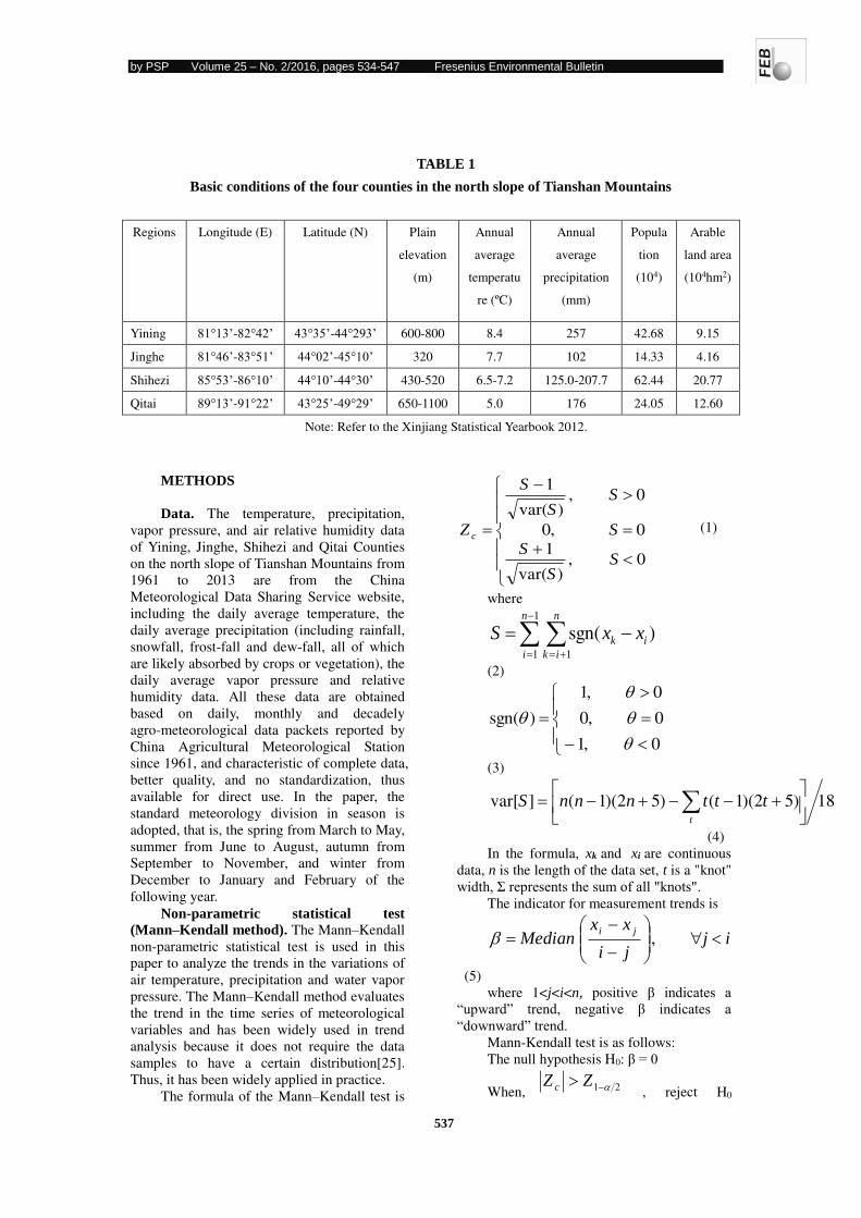
by PSP Volume 25 – No. 2/2016, pages 534-547 Fresenius Environmental Bulletin
537
TABLE 1
Basic conditions of the four counties in the north slope of Tianshan Mountains
Regions Longitude (E) Latitude (N) Plain
elevation
(m)
Annual
average
temperatu
re (ºC)
Annual
average
precipitation
(mm)
Popula
tion
(104)
Arable
land area
(104hm2)
Yining 81°13’-82°42’ 43°35’-44°293’ 600-800 8.4 257 42.68 9.15
Jinghe 81°46’-83°51’ 44°02’-45°10’ 320 7.7 102 14.33 4.16
Shihezi 85°53’-86°10’ 44°10’-44°30’ 430-520 6.5-7.2 125.0-207.7 62.44 20.77
Qitai 89°13’-91°22’ 43°25’-49°29’ 650-1100 5.0 176 24.05 12.60
Note: Refer to the Xinjiang Statistical Yearbook 2012.
METHODS
Data. The temperature, precipitation,
vapor pressure, and air relative humidity data
of Yining, Jinghe, Shihezi and Qitai Counties
on the north slope of Tianshan Mountains from
1961 to 2013 are from the China
Meteorological Data Sharing Service website,
including the daily average temperature, the
daily average precipitation (including rainfall,
snowfall, frost-fall and dew-fall, all of which
are likely absorbed by crops or vegetation), the
daily average vapor pressure and relative
humidity data. All these data are obtained
based on daily, monthly and decadely
agro-meteorological data packets reported by
China Agricultural Meteorological Station
since 1961, and characteristic of complete data,
better quality, and no standardization, thus
available for direct use. In the paper, the
standard meteorology division in season is
adopted, that is, the spring from March to May,
summer from June to August, autumn from
September to November, and winter from
December to January and February of the
following year.
Non-parametric statistical test
(Mann–Kendall method). The Mann–Kendall
non-parametric statistical test is used in this
paper to analyze the trends in the variations of
air temperature, precipitation and water vapor
pressure. The Mann–Kendall method evaluates
the trend in the time series of meteorological
variables and has been widely used in trend
analysis because it does not require the data
samples to have a certain distribution[25].
Thus, it has been widely applied in practice.
The formula of the Mann–Kendall test is
0,)var(
1
0,0
0,)var(
1
SS
S
S
SS
S
Z c
(1)
where
1
1 1
)sgn(n
i
n
ik
ik xxS
(2)
0,1
0,0
0,1
)sgn(
(3)
18)52)(1()52)(1(]var[
t
tttnnnS
(4)
In the formula, xk and xi are continuous
data, n is the length of the data set, t is a "knot"
width, Σ represents the sum of all "knots". The indicator for measurement trends is
ijji
xxMedian
ji
,
(5)
where 1<j<i<n, positive β indicates a “upward” trend, negative β indicates a “downward” trend.
Mann-Kendall test is as follows:
The null hypothesis H0: β = 0
When, 21 ZZ c , reject H0
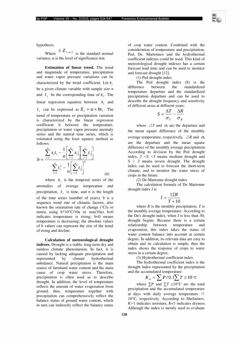
by PSP Volume 25 – No. 2/2016, pages 534-547 Fresenius Environmental Bulletin
538
hypothesis.
Where 21 Z is the standard normal
variance, α is the level of significance test.
Estimation of linear trend. The trend
and magnitude of temperature, precipitation
and water vapor pressure variations can be
characterized by the trend coefficient. Let ix
be a given climate variable with sample size n
and it be the corresponding time of ix . The
linear regression equation between ix and
it can be expressed asii btaX . The
trend of temperature or precipitation variation
is characterized by the linear regression
coefficient b between the temperature,
precipitation or water vapor pressure anomaly
series and the natural time series, which is
estimated using the least squares method as
follows:
2
11
2
111
1
1
n
i
i
n
i
i
n
i
i
n
i
i
n
i
ii
tn
t
txn
tx
b
(6)
where ix is the temporal series of the
anomalies of average temperature and
precipitation, it is time, and n is the length
of the time series (number of years). b is a
sequence trend rate of climatic factors, also
known the orientation rate of change (°C/a or
mm/a, using b*10°C/10a or mm/10a). b>0
indicates temperature is rising; b<0 means
temperature is decreasing; the absolute values
of b values can represent the size of the trend
of rising and decline.
Calculation of meteorological drought
indexes. Drought is a stable, long-term dry and
rainless climate phenomenon. In fact, it is
caused by lacking adequate precipitation and
represented by climate hydrothermal
unbalance. Natural precipitation is the main
source of farmland water content and the main
cause of crop water stress. Therefore,
precipitation is often used as to describe
drought. In addition, the level of temperature
reflects the amount of water evaporation from
ground, thus, temperature together with
precipitation can comprehensively reflect the
balance status of ground water content, which
in turn can indirectly reflect the balance status
of crop water content. Combined with the
consideration of temperature and precipitation,
Ped, De. Martonnex and the hydrothermal
coefficient indexes could be used. This kind of
meteorological drought indexes has a certain
forecast lead time and can be used to monitor
and forecast drought [12].
(1) Ped drought index
The Ped drought index (S) is the
difference between the standardized
temperature departure and the standardized
precipitation departure and can be used to
describe the drought frequency and sensitivity
of different areas at different years:
RT
RTS
where △T and σT are the departure and
the mean square difference of the monthly
average temperature, respectively, △R and σR
are the departure and the mean square
difference of the monthly average precipitation.
According to division by the Ped drought
index, 2 <S <3 means medium drought and
S > 3 means severe drought. The drought
index can be used to forecast the short-term
climate, and to monitor the water stress of
crops in the future.
(2) De Martonne drought index
The calculation formula of De Martonne
drought index I is
10
12
T
RI
where R is the monthly precipitation, T is
the monthly average temperature. According to
the De's drought index, when I is less than 30,
drought begins. Because there is a certain
relationship between temperature and
evaporation, this index takes the status of
water content balance into account at certain
degree. In addition, its relevant data are easy to
obtain and its calculation is simple, thus the
index shows the response of crops to water
stress in a certain degree.
(3) Hydrothermal coefficient index
The hydrothermal coefficient index is the
drought index represented by the precipitation
and the accumulated temperature:
101.0/ TPK w ℃
where ∑P and ∑T ≥10°C are the total
precipitation and the accumulated temperature
at days with daily average temperature ≥
10°C, respectively. According to Shelininov,
K>1 indicates moisture, K<1 indicates dryness.
Although the index is mostly used to evaluate
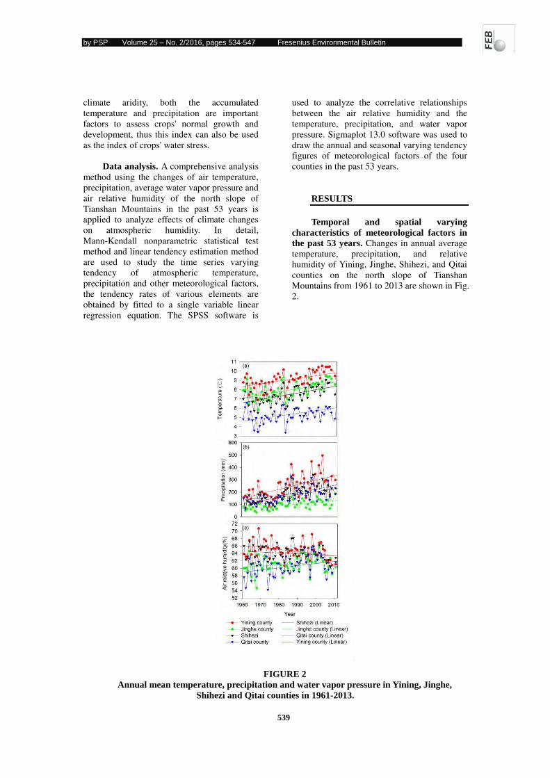
by PSP Volume 25 – No. 2/2016, pages 534-547 Fresenius Environmental Bulletin
539
climate aridity, both the accumulated
temperature and precipitation are important
factors to assess crops' normal growth and
development, thus this index can also be used
as the index of crops' water stress.
Data analysis. A comprehensive analysis
method using the changes of air temperature,
precipitation, average water vapor pressure and
air relative humidity of the north slope of
Tianshan Mountains in the past 53 years is
applied to analyze effects of climate changes
on atmospheric humidity. In detail,
Mann-Kendall nonparametric statistical test
method and linear tendency estimation method
are used to study the time series varying
tendency of atmospheric temperature,
precipitation and other meteorological factors,
the tendency rates of various elements are
obtained by fitted to a single variable linear
regression equation. The SPSS software is
used to analyze the correlative relationships
between the air relative humidity and the
temperature, precipitation, and water vapor
pressure. Sigmaplot 13.0 software was used to
draw the annual and seasonal varying tendency
figures of meteorological factors of the four
counties in the past 53 years.
RESULTS
Temporal and spatial varying
characteristics of meteorological factors in
the past 53 years. Changes in annual average
temperature, precipitation, and relative
humidity of Yining, Jinghe, Shihezi, and Qitai
counties on the north slope of Tianshan
Mountains from 1961 to 2013 are shown in Fig.
2.
FIGURE 2
Annual mean temperature, precipitation and water vapor pressure in Yining, Jinghe,
Shihezi and Qitai counties in 1961-2013.
Fig.2
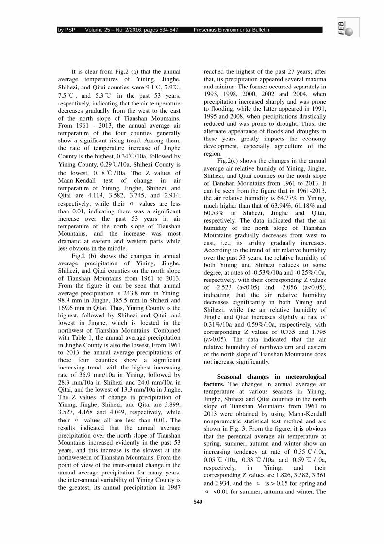
by PSP Volume 25 – No. 2/2016, pages 534-547 Fresenius Environmental Bulletin
540
It is clear from Fig.2 (a) that the annual
average temperatures of Yining, Jinghe,
Shihezi, and Qitai counties were 9.1℃, 7.9℃,
7.5℃ , and 5.3℃ in the past 53 years,
respectively, indicating that the air temperature
decreases gradually from the west to the east
of the north slope of Tianshan Mountains.
From 1961 - 2013, the annual average air
temperature of the four counties generally
show a significant rising trend. Among them,
the rate of temperature increase of Jinghe
County is the highest, 0.34℃/10a, followed by
Yining County, 0.29℃/10a, Shihezi County is
the lowest, 0.18℃ /10a. The Z values of
Mann-Kendall test of change in air
temperature of Yining, Jinghe, Shihezi, and
Qitai are 4.119, 3.582, 3.745, and 2.914,
respectively; while their α values are less
than 0.01, indicating there was a significant
increase over the past 53 years in air
temperature of the north slope of Tianshan
Mountains, and the increase was most
dramatic at eastern and western parts while
less obvious in the middle.
Fig.2 (b) shows the changes in annual
average precipitation of Yining, Jinghe,
Shihezi, and Qitai counties on the north slope
of Tianshan Mountains from 1961 to 2013.
From the figure it can be seen that annual
average precipitation is 243.8 mm in Yining,
98.9 mm in Jinghe, 185.5 mm in Shihezi and
169.6 mm in Qitai. Thus, Yining County is the
highest, followed by Shihezi and Qitai, and
lowest in Jinghe, which is located in the
northwest of Tianshan Mountains. Combined
with Table 1, the annual average precipitation
in Jinghe County is also the lowest. From 1961
to 2013 the annual average precipitations of
these four counties show a significant
increasing trend, with the highest increasing
rate of 36.9 mm/10a in Yining, followed by
28.3 mm/10a in Shihezi and 24.0 mm/10a in
Qitai, and the lowest of 13.3 mm/10a in Jinghe.
The Z values of change in precipitation of
Yining, Jinghe, Shihezi, and Qitai are 3.899,
3.527, 4.168 and 4.049, respectively, while
their α values all are less than 0.01. The
results indicated that the annual average
precipitation over the north slope of Tianshan
Mountains increased evidently in the past 53
years, and this increase is the slowest at the
northwestern of Tianshan Mountains. From the
point of view of the inter-annual change in the
annual average precipitation for many years,
the inter-annual variability of Yining County is
the greatest, its annual precipitation in 1987
reached the highest of the past 27 years; after
that, its precipitation appeared several maxima
and minima. The former occurred separately in
1993, 1998, 2000, 2002 and 2004, when
precipitation increased sharply and was prone
to flooding, while the latter appeared in 1991,
1995 and 2008, when precipitations drastically
reduced and was prone to drought. Thus, the
alternate appearance of floods and droughts in
these years greatly impacts the economy
development, especially agriculture of the
region.
Fig.2(c) shows the changes in the annual
average air relative humidy of Yining, Jinghe,
Shihezi, and Qitai counties on the north slope
of Tianshan Mountains from 1961 to 2013. It
can be seen from the figure that in 1961-2013,
the air relative humidity is 64.77% in Yining,
much higher than that of 63.94%, 61.18% and
60.53% in Shihezi, Jinghe and Qitai,
respectively. The data indicated that the air
humidity of the north slope of Tianshan
Mountains gradually decreases from west to
east, i.e., its aridity gradually increases.
According to the trend of air relative humidity
over the past 53 years, the relative humidity of
both Yining and Shihezi reduces to some
degree, at rates of -0.53%/10a and -0.25%/10a,
respectively, with their corresponding Z values
of -2.523 (a<0.05) and -2.056 (a<0.05),
indicating that the air relative humidity
decreases significantly in both Yining and
Shihezi; while the air relative humidity of
Jinghe and Qitai increases slightly at rate of
0.31%/10a and 0.59%/10a, respectively, with
corresponding Z values of 0.735 and 1.795
(a>0.05). The data indicated that the air
relative humidity of northwestern and eastern
of the north slope of Tianshan Mountains does
not increase significantly.
Seasonal changes in meteorological
factors. The changes in annual average air
temperature at various seasons in Yining,
Jinghe, Shihezi and Qitai counties in the north
slope of Tianshan Mountains from 1961 to
2013 were obtained by using Mann-Kendall
nonparametric statistical test method and are
shown in Fig. 3. From the figure, it is obvious
that the perennial average air temperature at
spring, summer, autumn and winter show an
increasing tendency at rate of 0.35℃ /10a,
0.05℃ /10a, 0.33℃ /10a and 0.59℃ /10a,
respectively, in Yining, and their
corresponding Z values are 1.826, 3.582, 3.361
and 2.934, and the α is > 0.05 for spring and
α <0.01 for summer, autumn and winter. The
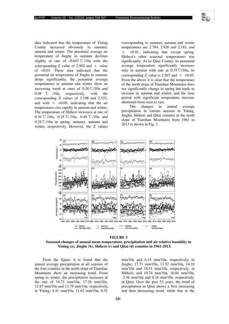
by PSP Volume 25 – No. 2/2016, pages 534-547 Fresenius Environmental Bulletin
541
data indicated that the temperature of Yining
County increased obviously in summer,
autumn and winter. The perennial average air
temperature of Jinghe in summer declines
slightly at rate of -0.043℃ /10a with the
corresponding Z value of 2.902 and α value
of <0.01. These data indicated that the
perennial air temperature of Jinghe in summer
drops significantly; the perennial average
temperatures in autumn and winter show an
increasing trend at rates of 0.36℃/10a and
0.48 ℃ /10a, respectively, with the
corresponding Z values of 3.108 and 2.523,
and with α <0.05, indicating that the air
temperatures rise rapidly in autumn and winter.
The temperature of Shihezi increases at rate of
0.36℃ /10a, 0.25℃ /10a, 0.49℃ /10a and
0.29℃ /10a in spring, summer, autumn and
winter, respectively. However, the Z values
corresponding to summer, autumn and winter
temperatures are 2.784, 2.926 and 2.183, and
α <0.01, indicating that except spring,
Shihezi's other seasonal temperatures rise
significantly. As to Qitai County, its perennial
average temperature significantly increases
only in autumn with rate at 0.35℃/10a, its
corresponding Z value is 2.507 and α <0.05.
From the above it is clear that the temperature
of the north slope of Tianshan Mountains does
not significantly change in spring but tends to
increase in autumn and winter, and the time
period with significant temperature increase
shortened from west to east.
The changes in annual average
precipitation in various seasons in Yining,
Jinghe, Shihezi and Qitai counties in the north
slope of Tianshan Mountains from 1961 to
2013 is shown in Fig. 3.
FIGURE 3
Seasonal changes of annual mean temperature, precipitation and air relative humidity in
Yining (a), Jinghe (b), Shihezi (c) and Qitai (d) counties in 1961-2013.
From the figure, it is found that the
annual average precipitation at all seasons of
the four counties in the north slope of Tianshan
Mountains show an increasing trend. From
spring to winter, the precipitation increases at
the rate of 14.73 mm/10a, 17.26 mm/10a,
12.87 mm/10a and 13.79 mm/10a, respectively,
in Yining; 4.41 mm/10a, 11.62 mm/10a, 8.52
mm/10a and 6.15 mm/10a, respectively, in
Jinghe; 17.71 mm/10a, 13.32 mm/10a, 14.18
mm/10a and 16.51 mm/10a, respectively, in
Shihezi; and 10.74 mm/10a, 16.84 mm/10a,
-3.36 mm/10a and 0.16 mm/10a, respectively,
in Qitai. Over the past 53 years, the trend of
precipitation in Qitai shows a first increasing
and then decreasing trend, while that in the
by PSP Volume 25 – No. 2/2016, pages 534-547 Fresenius Environmental Bulletin
542
other three counties show an increasing trend.
The non-parametric statistical tests of
precipitation data at different seasons in the
four counties found that the Z values of winter
precipitation were 1.969, 2.467, 2.981 and
3.068, respectively in Yining, Jinghe, Shihezi
and Qitai and their corresponding α was
<0.05, indicating that winter precipitation
significantly increases over the past 53 years
and the autumn precipitations in Shihezi also
increased with corresponding Z-value of 1.977.
Overall, the increased precipitation in the north
slope of Tianshan Mountains is mainly
concentrated in winter.
The annual variations of the annual air
relative humidity at various seasons from 1961
to 2013 in Yining, Jinghe, Shihezi and Qitai
counties are shown in Fig.3. It is found that the
spring, summer and winter air relative
humidity of Yining county and the spring,
summer, autumn and winter air relative
humidity of Shihezi showed an decreased trend,
while that of the summer, autumn of Jinghe
county and the spring and summer of Qitai
county tended a slightly increasing tendancy.
The non-parametric statistical tests showed
that the Z-values were -3.345, -2.143 and
4.642, respectively, for the air relative
humidity trend in spring, summer of Yining,
summer of Qitai and their a was <0.05. The
data indicated that the spring and summer air
relative humidity of Yining county
significantly decreased, the summer air relative
humidity of Qitai county increased
significantly while that of the other seasons of
other counties did not change significantly.
Calculations on drought indexes on the
north slope of Tianshan Mountains. The arid
conditions of the north slope of Tianshan
Mountains over the past 53 years were
quantitatively calculated using the
comprehensive indexes as the Ped drought
index, De. Martonne drought index, and
hydrothermal coefficient indicator that are
commonly affected by temperature and
precipitation.
In Fig.4, S values show the calculated
Ped drought index.
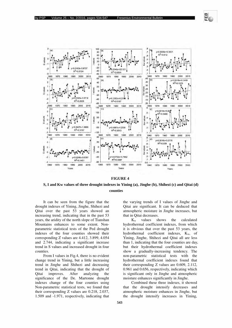
by PSP Volume 25 – No. 2/2016, pages 534-547 Fresenius Environmental Bulletin
543
FIGURE 4
S, I and Kw values of three drought indexes in Yining (a), Jinghe (b), Shihezi (c) and Qitai (d)
counties
It can be seen from the figure that the
drought indexes of Yining, Jinghe, Shihezi and
Qitai over the past 53 years showed an
increasing trend, indicating that in the past 53
years, the aridity of the north slope of Tianshan
Mountains enhances to some extent. Non-
parametric statistical tests of the Ped drought
indexes of the four counties showed their
corresponding Z values are 4.412, 3.899, 4.054
and 2.744, indicating a significant increase
trend in S values and increased drought in four
counties.
From I values in Fig.4, there is no evident
change trend in Yining, but a little increasing
trend in Jinghe and Shihezi and decreasing
trend in Qitai, indicating that the drought of
Qitai improves. After analyzing the
significance of the De. Martonne drought
indexes change of the four counties using
Non-parametric statistical tests, we found that
their corresponding Z values are 0.218, 2.037,
1.509 and -1.971, respectively, indicating that
the varying trends of I values of Jinghe and
Qitai are significant. It can be deduced that
atmospheric moisture in Jinghe increases, but
that in Qitai decreases.
Kw values shows the calculated
hydrothermal coefficient indexes, from which
it is obvious that over the past 53 years, the
hydrothermal coefficient indexes, Kw, of
Yining, Jinghe, Shihezi and Qitai all are less
than 1, indicating that the four counties are day,
but their hydrothermal coefficient indexes
show a gradually-increasing tendency. The
non-parametric statistical tests with the
hydrothermal coefficient indexes found that
their corresponding Z values are 0.609, 2.112,
0.961 and 0.656, respectively, indicating which
is significant only in Jinghe and atmospheric
moisture enhances significantly in Jinghe.
Combined these three indexes, it showed
that the drought intensify decreases and
atmospheric moisture enhances in Jinghe, but
the drought intensify increases in Yining,
Fig.4
by PSP Volume 25 – No. 2/2016, pages 534-547 Fresenius Environmental Bulletin
544
Shihezi and Qitai.
DISCUSSIONS
Response of regional climate on the
global warming. Response of the climate in
the different regions on the global warming is
different. Studies have found that in China,
compared with the 1990s, the winter air
temperature of the Yangtze River after 2000
reduces, while the summer air temperature
rises. In addition, precipitation in Yangtze
River reduces and air becomes dry[26]. Zhang
et al[27]showed that a significant increasing
trend of 7.40 mm/10a in the annual mean
precipitation and an increasing trend of
0.25 ℃ /10a in the annual maximum
temperature in Xinjiang, northwest of China
during 1961-2008. Moreover, the air
temperature of the Tarim River Basin located
in the southern Xinjiang also showed an
increasing trend[28]. Su et al. [29]studied the
climate conditions of the north slope of
Tianshan Mountains over the past 40 years and
found that the air temperature and precipitation
of this region increase, especially in its plain
oases. However, previous studies on the north
slope of Tianshan Mountains climate mainly
focused on its mountainous regions and plains
oases. In this study, we focus on the climate
changes of its typical four counties from west
to east over the past 53 years. Our studies
found that with the global climate warming,
the temperature and precipitation in the north
slope of Tianshan Mountains show a
significant increasing trend, which is
consistent with the conclusions from previous
researches. However, different counties show
different changes in their climate situations.
The air temperature and precipitation of Yining
located in the west of the north slope of
Tianshan Mountains increase the fastest, while
those of Qitai in the east increases only slightly.
In addition, the original temperature and
precipitation of Yining County are higher than
other counties', as shown in Fig.2, thus it can
be referred that in the next several years, the
air temperature, precipitation and atmosphere
humidity of Yining county on the entire
northern slope of Tianshan Mountains remain
the greatest.
Regional drought. We found that both
temperature and precipitation in the north
slope of Tianshan Mountains increased
evidently over the past 53 years. However, the
air relative humidity decreases obviously in
Yining and Shihezi, and that enhances in
Jinghe and Qitai. Although the air temperature
and precipitation increased on north slope of
Tianshan Mountains over the past 53 years,
analyses of their seasonal variation found that
these two phenomena occurs mainly in autumn
and winter, during which periods the air
temperature is lower and evaporation is weaker.
Even if the precipitation increases, the vapor in
air over Shihezi is mostly present in the forms
of snow and ice, whose evaporation is weaker
at low temperature, resulting in a decline in the
vapor content in the air. While in short and hot
summer, the air temperature, but not
precipitation rises, thus the evaporated
moisture is still less, resulting in no significant
changes in annual atmospheric humidity. That
is why the air relative humidity decreases
obviously in Yining and Shihezi in the past 53
years. The conclusion is in an agreement with
the conclusions of Jung and Chang et al
(2012)[4] that precipitation increase in winter
would not change the long-term arid situation.
In other words, precipitation increase in winter
would not increase overall annual air relative
humidity. In Yining County, winter and spring
are warm and humid, ice and snow are easy to
melt; at a lower temperature, melted snow
water mostly seeps into the ground and
becomes groundwater and only a small amount
of snow water is evaporated; while its summer
and autumn are dry and hot, thus only the air
temperature, but not the precipitation rises.
Therefore, the evaporated vapor doesn't
increase, showing a declining trend in the air
humidity. Jinghe's precipitation in autumn and
winter increases significantly, while in spring
the air temperature increases rapidly[25]. Thus,
large amount of surface snow water is
evaporated, resulting in enhancements in both
the vapor content and air humidity.
Atmospheric drought refers to water
shortages in a certain period of time due to
imbalances of evaporation and precipitation
and excessive water expenditures over water
revenue. Atmospheric drought is the
forerunner of agricultural and hydrological
drought and will affect the latter. In recent
decades, although the precipitation on the
north slope of Tianshan Mountains has
increased, its temperature also rises, leading to
intense evaporation and subsequent higher
evaporation capacity than precipitation ability,
which is reflected in the atmosphere as
decreased humidity and increased aridity. Our
analyses found that the air relative humidity
by PSP Volume 25 – No. 2/2016, pages 534-547 Fresenius Environmental Bulletin
545
decreased in Yining County and Shihezi but
did not change significantly in the other two
counties. These data indicated that the overall
atmospheric aridity increased in the north
slope of Tianshan Mountains. Water moisture
expenditures exceeded revenue will cause soil
water deficit, destroy water equilibrium in
corps and affect corps’ normal physiological
activity, leading to agricultural drought
occurrence [30]. With the increase in water
evaporation capability, water in river will be
significantly evaporated, which will result in
no significant changes in river runoff and
eventually lead to hydrological drought.
Measures to alleviate atmospheric
drought. Air humidity decrease in Yining may
be related to increased human activities and
decreased water resource. First of all, decrease
in soil and water conservation function and
climate regulation in the north slope of
Tianshan Mountains are caused by the serious
forest shrinkage, grassland degradation,
mountain ecosystems destruction due to
human’s long term unreasonable utilization of
forest and pasture resources. Secondly, soil
erosion and swamp salinization are caused by
lack of long term planning in water
conservancy construction, incomplete support
of some facilities, and disadvantageous
management measures. Thirdly, dramatic
increase in river use also accelerates soil
erosion, marshes salinization and other issues.
In addition, with the increase of population,
and the continuous development of industry
and agriculture productions, water use for
irrigation, production and normal life increases
more and more. Reduction of water resource
and increases in arid severity lead to frequent
occurrence of natural disasters in Yining
County [31] From Fig.2 it is clear that since
the 1990s, the county has been repeatedly and
alternatively suffered from floods and droughts.
Drought occurs once every 3-4 years in spring,
leading to water shortage of arable land and
poor farmland humidity that delays timely
sowing as well as normal growth of crops and
flowering of fruit trees, every 2-3 years in
summer at crops' vigorous growth period,
greatly affecting crops growth, every 3-4 years
in autumn at crops' seed-filling period, greatly
affecting crops maturation, timely winter
wheat and other crops planting and pre-winter
crops growth and development[32]. Floods and
droughts all will result in agricultural
underproduction and even serious economic
losses. Therefore, it is appropriate for Yining
County to reduce the arable land for grassland
and pasture, doing so not only can reduce the
loss caused by crops underproduction, but also
can promote the development of local animal
husbandry as well as alleviate and delay
serious ecological environment damage.
CONCLUSIONS
With global climate warming, various
regions of the north slope of Tianshan
Mountains, Xinjiang, China, showed different
responses. Analyses of spatial and temporal
variation characteristics of the 1961-2013
perennial average air temperature, annual
precipitation, water vapor pressure, and air
relative humidity found that various counties
on the north slope of Tianshan Mountains
showed trends of temperature rising and
precipitation increasing. However, the water
vapor pressure and air relative humidity
showed different trends. Except for Yining
County in the west of the north slope of
Tianshan Mountains, the vapor pressures of
Jinghe, Shihezi and Qitai located respectively
in the northwest, center and east all
significantly increased. However, a rise in the
vapor pressure does not mean an increase in
the air relative humidity, which is also related
to the saturated vapor pressure. This study
found that the air relative humidity in Yining
and Shihezi reduced to some extent, which
may be because precipitation often increases in
fall and winter, which will not lead to increase
in annual air relative humidity.
In order to solve the drought tendency,
one should appropriately reduce the area of
arable land and increase the area of forests and
pasture, such doing can not only reduce the
loss due to crops underproduction, but also
promote the development of local animal
husbandry and alleviate and delay serious
ecological environment damage.
ACKNOWLEDGEMENTS
We were grateful for the China
Meteorological Data Sharing Service website
because of the climate data provided. This
study was supported financially by the Project
of Scientific and Technological Personnel
Training of Young Doctor in Autonomous
Region (Grant No. 2013731025, 2013721050)
and National Natural Science Foundation of
China (Grant No.41271052).
by PSP Volume 25 – No. 2/2016, pages 534-547 Fresenius Environmental Bulletin
546
AUTHOR CONTRIBUTIONS
Aihong Fu made all the figures and tables
and wrote the whole manuscript.
Yaning Chen conceived and designed the
experiments.
Weihong Li analyzed the data.
CONFLICTS OF INTEREST
The authors declare no conflict of interest.
The founding sponsors had no role in the design
of the study; in the collection, analyses, or
interpretation of data; in the writing of the
manuscript, and in the decision to publish the
results.
REFERENCES
[1] Li, M.S., Li, S., Li, Y.H. Studies on
drought in the past 50 years in China.
Agricul. Meteor., 2003, 24(1):8-11.
[2] Mengu G. P., Anac S., Topcuoglu K.
Analysis of drought in the Marmara
region using the Standardized
Precipitation Index. Fresenius
Environmental Bulletin,
2009,18(5):633-641.
[3] Mengu G. P., Akkuzu E., Anac S., et al.
Impact of climate change on irrigated
agriculture. Fresenius Environmental
Bulletin, 2011,20(3A):823-830.
[4] Jung, W., Chang, H.J. Climate change
impacts on spatial patterns in drought risk
in the Willamette River Basin, Oregon,
USA. Theor Appl. Climatol., 2012, 108:
355-371.
[5] Usta A., Yilmaz M., Malkocoglu S., et al.
Effects of environmental factors on wood
anatomy of black alder (Alnus glutinosa
(L.) Gaertner subsp barbata (CA Meyer)
Yalt) from two different origins of eastern
black sea region in Turkey. Fresenius
Environmental Bulletin,
2014,23(8):1778-1784.
[6] Zou, W.X., Yang, C.B., Jiang, H., Han,
X.Z. The effect of long-term fertilization
on soil water dynamics and water use
efficiency in a field experiment of black
soil region in northeast China. Fresenius
Environmental Bulletin, 2014:
23(3):840-850.
[7] Chun, K.P., Wheater, H., Onof, C.
Prediction of the impact of climate
change on drought: an evaluation of six
UK catchments using two stochastic
approaches. Hydrol. Processes, 2013,
27(11):1600-1614.
[8] Raje, D., Mujumdar, P.P. Hydrologic
drought prediction under climate change:
Uncertainty modeling with
Dempster-Shafer and Bayesian
approaches. Adv. Water Resour,
2010,33:1176-1186.
[9] Vrochidou, A.E.K., Tsanis, I.K., Grillakis,
M.G., Koutroulis, A.G. The impact of
climate change on hydrometeorological
droughts at a basin scale. J. Hydrol.,
2013,476:290-301.
[10] Kim, C.J., Park, M.J., Lee, J.H. Analysis
of climate change impacts on the spatial
and frequency patterns of drought using a
potential drought hazard mapping
approach. Int. J. Climatol.,
2014,34(1):61-80.
[11] Lee, J.H., Kim, C.J. A multimodel
assessment of the climate change effect
on the drought
severity-duration-frequency relationship.
Hydrol. Processes, 2013,
27(19):2800-2813.
[12] Liu, Z.Y., Zhang, J.P., Luo, H.X., He, Y.K.
Temporal and spatial distribution of
maize drought in Southwest of China
based on agricultural reference index for
drought. Transac. Chin. Soc. Agricul.
Engin., 2014, 30(2):105-115.
[13] Bao, Y.S., Yan, J., Min, J.Z., Wang, D.M.,
Li, Z.T., Li, X.C. Agricultural drought
monitoring in north Jiangsu by using
temperature vegetation dryness index. .
Transac. Chin. Soc. Agricul. Engin., 2014,
30(7):163-172.
[14] Lu, H.J., Mo, X.G., Hu, S. Spatiotemporal
variation characteristics of meteorological
droughts in North China Plain during
1960-2009. J. Nat. Dis., 2012,
21(6):72-82.
[15] Zhao, L. Analysis on temporal and spatial
variation of agricultural meteorological
drought in agricultural area in Qinhai
province. Master Degree, Northwest
Agriculture and Forestry University,
Shaanxi, China, 2010.
[16] Wang, P.Y., Li, Z.Q., Jin, S., Zhou, P., Yao,
H.B., Wang, W.B. Ice thickness, volume
and subglacial topography of Urumqi
Glacier No.1, Tianshan Mountains,
central Asia, by ground penetrating radar
survey. J. Earth System Sci., 2014,
123:581-591.
by PSP Volume 25 – No. 2/2016, pages 534-547 Fresenius Environmental Bulletin
547
[17] Bai, J., Chen, X., Li, J.L., Yang, L., Fang,
H. Changes in the area of inland lakes in
arid regions of central Asia during the
past 30 years. Environ Monit. Assess,
2011,178: 247–256.
[18] Cao, Y.J., Yan, J.P. Changes in climate and
climatic productivity in Jinghe county of
Xinjiang during last 56 years. Res. Devel.
Market, 2012, 28(3):267-269.
[19] Song, W.J., Xiong, H.G., Qi R. Climate
change in Qitai County in Xinjiang in
recent 42 a. J. Arid Land Resour. Environ.,
2009, 23(4):100-106.
[20] Guo, J.Q., Wang, X.J. Analysis on climate
change in recent 50 years in Shihezi
Prefecture, Xinjiang. Qinhai Climate,
2011, 4: 46-51.
[21] Ling, H.B., Xu, H.L., Fu, J.Y. Temporal
and spatial variation in regional climate
and its impact on runoff in Xinjiang,
China. Water Resour. Manag,
2013,27:381-399.
[22] Wang, H.J., Chen, Y.N., Li, W.H., Deng
H.J. Runoff responses to climate change
in arid region of Northwestern China
during 1960-2010. Chin. Geogra. Sci.
2013, 23(3):286-300.
[23] Li, B.F., Chen, Y.N., Chen, Z.S., Li, W.H.
Trends in runoff versus climate change in
typical rivers in the arid region of
northwest China. Quatern. Int.,
2012,282:87-95.
[24] Li, Q. Drought leads to extreme withering
in Aibi River, Xinjiang.
http://www.ts.cn/homepage/content/2008-
09/11/content_3027645.htm.2008.9.11.
[25] Wang, Y.H. The harm of sand and
prevention measures in Jinghe county.
Environmental Protection of Xinjiang,
1997, 19(2):5-9.
[26] Wang, Y.G., Gong, Z.S., Xu, L., Ai, W.X.
Analysis of long trend of temperature and
precipitation in China and its influencing
factors. Q. J. Appl. Meteorol.,
2005,16(supI):85-90.
[27] Zhang, Y., Wei, W., Jiang, F., Liu, M.,
Wang, W., Bai, L., and Li, K. Brief
communication "Assessment of change in
temperature and precipitation over
Xinjiang, China", Nat. Hazards Earth
Syst. Sci., 2012, 12, 1327-1331,
[28] Liang, L.G. Xinjiang Tarim River Basin
temperature, precipitation and runoff
characteristics and trend. Yellow River,
2014, (8).
[29] Su, L.T., Song, Y.D., Zhang, Z.Y.
Response of the climate and ecological
environment in Northern Slope of
Tianshan Mountains to global warming
since recent 40 years. Arid Land Geog.,
2005, 28(3):342-346.
[30] He, L.K. Problems and measures on water
and soil conservation in Yining county in
Xinjiang. Heilongjiang Sci. Technol.
Water Conser., 2013, 41(11):230-232.
[31] http://www.cma.gov.cn/kppd/kppdqxwq/
kppdjckp/201211/t20121128_192964.ht
ml. Types of drought and their
relationship. Chinese Meteorological
News, 2011,5.25.
[32] Lei, J., Ma, Y.P. Analysis of agricultural
climate resources in Yining county and the
main meteorological disasters. Mod. Agr.
Tech., 2011, 22:305,312.
Received: 21.07.2015
Accepted: 16.12.2015
CORRESPONDING AUTHOR
Aihong Fu
State key laboratory of desert and oasis
ecology
Xinjiang Institute of Ecology and Geography
Chinese Academy of Sciences
CHINA
e-mail: [email protected]
by PSP Volume 25 – No. 2/2016, pages 548-564 Fresenius Environmental Bulletin
548
THE CHARACTERISTICS OF SOIL WATER
EVAPORATION IN THE CORN FIELDS UNDER
DIFFERENT CLIMATE CONDITIONS IN ARID REGIONS
OF NORTHWESTERN CHINA
Aihong Fu1,2, Weihong Li1, Yaning Chen1
1. State Key Laboratory of Desert and Oasis Ecology, Xinjiang Institute of Ecology and Geography, Chinese Academy of
Sciences, 818 South Beijing Road, Urumqi 830011, China
2. The Department of Geography, University of California, Los Angeles, UCLA, California, CA90095, USA.
ABSTRACT
Studying the responses of water
evaporation rate to climate changes in corn fields
located in arid regions can effectively provide
the scientific basis for the formulation of the
appropriate irrigation strategies and for
increasing the efficient use of water resources. In
this study, three representative climate regions
located in Yanqi, Shanshan and Qinghe Counties
in the arid regions in northwest of China were
studied to investigate the indicative threshold
values of the environmental factors that cause
significant changes in soil water evaporation rate
in corn fields in the summer by monitoring
on-site the daily changes in soil water
evaporation rate in corn fields, liquid flow rate in
corn stalks, water content within 1m-soil layer
underneath topsoil, and the meteorological
factors including air temperature (Tair),
atmosphere relative humidity (RH), and wind
velocity (Wv). The study results indicated: (1)
when soil water content was higher, a
phenomenon of short “Afternoon break” in
water evaporation existed in the corn fields in
Shanshan and Yanqi Counties where mean
annual Tair was higher but this phenomenon did
not exist in corn fields in Qinghe County where
mean annual Tair was lower. There existed a
phenomenon of no-liquid flow and transpiration
in corn evaporation rate at noon. High
temperature was favorable for corn growth.
When soil water content was lower, no
“afternoon break” existed in soil water
evaporation in corn field and corn transpiration
rate in three counties. Low temperature was
favorable for corn growth; (2) there were
significant correlations between soil water
evaporation rate in corn fields and Tair, Wv, soil
temperature (Ts) and RH. There were significant
correlations of corn transpiration rate with Ts,
RH and Tair; (3) Temperature at 22.59℃ was the
minimum threshold for Ts that affected the
changes in corn transpiration rate. When soil
water content was 22.73%, corn respiration rate
was the highest. Planting two rows of crops with
higher height such as sorghum and sunflowers in
outside boundary of corn fields, simultaneously
controlling irrigation frequencies and irrigation
amounts and increasing Ts and RH to maintain
soil water content at about 22.73%, may be the
effective ways to reduces soil water evaporation
rate and increase corn transpiration rate.
KEY WORDS:
Soil evaporation rate; transpiration rate; corn; climate
changes; arid region.
INTRODUCTION
The global climate changes are mainly
characterized by the persistently warming
climate and frequent incidences of extreme
weather conditions, which have threatened the
survival and development of human beings.
From the agricultural perspective, the warming
climates have already led to the corresponding
changes in plantation timing, cycle, locations
and varieties for a part of crops, acceleration of
crop growth and development and the shortening
of the crop growth and developmental stages,
which did not allow crops to have sufficient time
for full formation of their grains and thus
gradually reduced crop yields. The instability for
agricultural production has been increased and
has even forced the adjustment of the structure
and patterns for crop plantation. The food crop
production in various countries in the world has
been reduced to varying extends. For instance,
since the start in 2003, the major food-producing
countries in the world, such as Australia,
by PSP Volume 25 – No. 2/2016, pages 548-564 Fresenius Environmental Bulletin
549
Ukraine and Canada etc., have continuously
suffered from the natural disasters and their food
production has been reduced. According to the
statistical data, during the period of 2004 to 2006,
due to the drying climate and other factors, the
total wheat yield in Australia was reduced by
52%, the food production in the United States
was reduced by 13%, and the food production in
European Unions was reduced by 14%, which
had directly impacted the amounts of food
storage in a number of countries. Many countries
and even those countries that used to export food
have become the food-importing ones. In Asia, it
has been estimated that the climate changes in
the future will have significant impacts on
agricultural production through the continuing
reduction of crop yields and the shrinkage of
cultivatable areas[Mengu et al., 2009].
Warming climate has already caused
significantly negative impacts on agricultural
production in China. Climate warming has led to
a trend of the exaggerated fluctuation of crop
production in China due to the increased drought
areas caused by the drought disaster [Zhou
2001]. The influences on the agricultural
production patterns and structures in China
caused by the climate changes will further
increase the cost of agricultural production in the
future [Ma et al. 2011].
The studies of the impacts of climate
changes on agricultural production have
attracted increasing and broad attentions.
Regarding the studies about the impacts of
climate changes on soil water evaporation, many
investigators have investigated the differences in
the soil water evaporation rate in corn field
under different plantation patterns to find out the
key factors that influence the soil water
evaporation rate [Wang et al. 2004]. Among
which, the water contents in the 0-30 cm soil
layer and the temperature in the 0-25 cm soil
layer displayed a significantly positive
correlation with the daily soil water evaporation
rate [Chai et al. 2011]. The daily changes in soil
water evaporation rate in winter wheat field
displayed in single-peak trend and the peak
value occurred in the period between 12:00 and
14:00 PM. At the same time, there was a good
linear correlation between the proportion of soil
water evaporation in relative to the ratio of
evaporation to transpiration and the water
content in topsoil. Rainfall and irrigation also
caused relatively large impacts on soil water
evaporation rate [Liang et al. 2011]. By
applying the climate-related factors such as soil
temperature etc., a number of studies have
estimated the soil water evaporation rates for
different crops [Gunnel and Per-Erik 1997
Bittelli et al., 2008 Kerridge et al., 2013 Qiu
et al., 2006 Yamanake and Yonetani 1999
Aydin et al., 2005 Tapan et al., 2001; Wallace
et al., 1999]. In term of the studies on the
impacts of climate changes on the transpiration
rates of crops, it has been found that the daily
changes in the transpiration rate of winter wheat
displayed a single-peak trend and the peak value
occurred during the period between 12:00 and
14:00 PM and the transpiration rate was
increased with the increase in air temperature
(Tair) [Liang et al. 2011]. Under the situation
when the agricultural technologies were not
changed, the higher the latitude was, the larger
the impact of Tair on the transpiration rate of food
crops and the lower the latitude was, the smaller
impact. In the areas located in the middle
latitude, the disturbance by solar radiation after
irrigation caused huge changes in transpiration
rate [Terjung et al., 1984]. The global warming
climate can stimulate the growth of plants in the
middle and high latitude areas but can cause
negative impacts on the growth of plants in arid,
semi-arid and tropical regions [Samsul Huda et
al., 1993; Usta et al., 2014]. For example, in the
United States, with the increase in Tair, the
growth of crops in northern areas was stimulated
whereas the growth of crops in southern areas
was reduced [Southworth et al., 2002]. The
climate changes can reduce the soil fertility,
destroy soil structures and reduce the soil
retention capacity and thus, reduce the crop yield
but the increase in Tair, rainfall and CO2
concentration increased crop yields [Samsul
Huda et al., 1993; Mengu et al., 2011].
It can be seen from what have been
mentioned above that a number of domestic and
foreign investigators have conducted numerous
studies on the response of crop
evapotranspiration to climate changes. However,
most of these studies have mainly focused on
investigating the impacts of Tair, rainfall and
irrigation on the evapotranspiration and crop
growth in a macro-scale and have paid their
attention to the response of evapotranspiration of
winter wheat and the amount of transpiration in
the humid areas to the different changes in
climate and the methods for measurement of the
evapotranspiration of summer corn. However,
these studies have not investigated the
characteristics in the daily changes in
evapotranspiration in corn field in the summer
under different climate conditions in arid regions
and on their influencing factors and thus, the
threshold limit values for the environmental
factors indicative for the changes in the
by PSP Volume 25 – No. 2/2016, pages 548-564 Fresenius Environmental Bulletin
550
evapotranspiration of the summer corn have not
been available. In this study, the summer corn
fields in three representative climate regions in
Yanqi County, Shanshan County and Qinghe
County located in the arid areas in Xinjiang
Uygur Autonomous Region in northwest of
China were selected to investigate the
characteristics of the daily changes in the soil
water evaporation rate and corn transpiration
rate in the summer corn fields and to analyze the
predominant environmental factors that cause
significant influences on the evapotranspiration
in the summer corn field and their threshold
limit values, aiming to provide the scientific
basis for effectively formulating the appropriate
strategies for irrigation of the corn fields in arid
regions.
STUDY AREA AND METHODS
STUDY AREA
In this study, three counties representing
the middle and south parts (Yanqi County),
eastern part (Shanshan County) and the northern
part (Qinghe County) in Xinjiang Uygur
Autonomous Region were studied Fig.1 , These
three counties have quite different climates.
Yanqi County
(E85°13′-86°44′,N41°45′-42°20′) is located at
the center of Yanqi Basin at the south foothill of
Tianshan Mountain in Xinjiang. Its southeast is
bordered by Bohu County, its north is connected
to Hejing County, its northeast is linked to
Heshuo County, its south is faced by Korla City
and its southwest is bordered by Luntai County.
Its topography is such that its northwestern part
is high and its southeastern part is low. The
Kaidu River traverses its eastern part, Konqu
River flows across its south part. There are small
wetlands in its middle part. Its total area is
2570.88 km2, and its total population (in 2004)
was 120 thousands. There are a total of 23
nationalities including Hui, Han, Uygur and
Mongolian nationalities in this county.
Traditionally, Yanqi County is an agricultural
area. More than 70 crops are currently grown
and the major crops are wheat, corn, rice, broad
bean and Pijiuhua etc. The economic crops with
the local characteristics include fennel, red
pepper, Chinese cabbage, white sunflower,
tomato, beet, grape, and wild licorice root etc.
The climate in Yanqi County belongs to
temperate continental drying climate. It is very
hot in the summer but is extremely cold in the
winter. The climates are buffered by the water in
Bosten Lake. Thus, there are no vigorous
variations in cold-hot weather conditions. The
day-time radiation is longer and the thermality is
abundant. The annual available sunshine hours
are 4440.1 hours and the total annual solar
radiation is 156.84 thousand Cal/cm2, being
ranked the second highest among those in all
counties in Xinjiang. The mean annual
biologically acquirable solar radiation per unit
area is 78400 Cal/cm2 being ranked the first
place among those in all the counties in Xinjiang.
The mean annual non-frost period is 176 days
and the mean annual precipitation (rainfall) is
74.4 mm. The mean annual Tair is 8.2oC the
extremely high temperature is 38℃ and the
extremely low temperature is -35℃. The most
frequent wind direction is the northwest wind.
Shanshan County (E90°21′-90°25′, N42°82′-42°86′) is located in the Asian
innermost at the middle latitude at the eastern
side of Turpan Basin at the south foothill of the
eastern part of Tianshang Mountain. It north is
neighbored by Mulei County and Qitai County.
Its east is connected via Qiketai town to
Qijiaojing Town of Kumul (or Hami). Its west is
bordered by Subashi village in Toyukmazar and
the Shangjinxiang County in Turpan City. Its
south is bound by Ruoqiang County and Yuli
County via Nanhu (South Lake) Gobi Desert
through Jiaoluotage Mountain. The total area of
this county is 39800 km2, accounting for 2.5% of
the total area of Xinjiang. Agriculture is the
major economic source for Shanshan County. In
addition to grape, melon and cotton, the other
crops include wheat, corn, white sorghum and
vegetables, beans, tuber crops, grass pasturage,
and fruit etc., which are usually sporadically
planted or inter-planted or multiply-cropped but
the plantation areas for these crops are small.
Because Shanshan County is far away from the
seas/oceans and is surrounded by mountains, its
topography is complex. Its climate belongs to
the temperate continental drying climate. It is
extremely hot in the summer but is extremely
cold in the winter. The diurnal temperature
difference is big. The solar radiation during the
daytime is abundant. The mean annual Tair is
11.3℃. The mean annual precipitation (rainfall)
is 25 mm. The temperature in summer is hot, the
mean Tair in July is 29.2~33℃ and there has
been the occurrence of the extremely high
temperature of 48℃. The temperature in the
winter is extremely cold. The mean Tair in
January is -10~11℃. The lowest temperature
that used to occur was -28.7~ -29.7℃. The
by PSP Volume 25 – No. 2/2016, pages 548-564 Fresenius Environmental Bulletin
551
spring is the drying season. The annual
precipitation (rainfall) is 17.6~25.3 mm but the
evaporation rate is extremely high, which is
2751~3216.6 mm. The thermality is abundant.
The accumulated temperature at ≥10℃ is
4522.6~5548.9℃. The daytime solar radiation
is plenty. The day-time solar radiation hours are
2900~ 3100 hours. The diurnal temperature
difference is big, which is 14.3~15.9℃ and can
reach as big as 17~26.6℃. The non-frost period
is long, which is 192~224 days. These climate
conditions are favorable for the growth and
development of cotton, grape and sweet water
melon and are particularly favorable for
improving the quality of grape and sweet water
melon.
Qinghe County (E90°37′, N46°71′) is
located at the northeastern edge of Dzungarian
Basin and the southeastern foothill of Altai
Mountains. Its west is neighbored by Fuyun
County and its south is linked by Qitai County in
Changji. Its northeast is bordered by the country
of Mongolian. The length of its boundary line is
282 km and the total area is 15700 Km2. Qinghe
County administers five village districts and two
towns, 54 administrative villages and its total
population is 63.2 thousands (in 2008), which is
consisted of 16 nationalities including Kazak,
Han, Mongolian, Hui and Uyghur nationalities.
Within Qinghe County, the soil is fertile and
there are 133.332 km2 of cultivatable land and
the total exportable areas are as high as 1066.656
km2. Qinghe County is the major food-producing
county in Xinjiang. Wheat is the major
agricultural crop in Qinghe County. In addition
to wheat, rape, white peas and corn are also
grown. The topography within Qinghe County is
located in the area of high above sea level and
high latitude. The highest above sea level is
3659 m and the lowest above sea level is 900 m.
The extremely low air temperature is -53℃, and
the mean annual Tair is 0℃. The mean annual
precipitation is 161 mm, the evaporation rate can
reach as high as 1495 mm The mean non-frost
period is 103 days and the shortest annual
non-frost period is 87 days. The climate
conditions are abominable and the natural
disasters have occurred frequently.
METHODS
Experimental Designs. According to the
regional climate characteristics, three counties
including Yanqi County, Shanshan County and
Qinghe County representing the typical climate
regions within the boundary of Xinjiang were
selected for this study. Among three counties, the
mean annual Tair in Shanshan County is the
highest one and its precipitation is the lowest
one and is a typical arid-hot area. The mean
annual Tair in Qinghe County is the lowest one
but its precipitation is the highest one and is a
typical humid-cold climate area. The thermality
and humidity in Yanqi County are between those
of Shanshan County and Qinghe County. In
April 2012, in the distance of 5-8 km from the
outside of the county region, six corn fields,
where the growth and development of corn are
normal and the levels of irrigation are the same
but the intervals of irrigation are different, were
selected for conducting this study. Two corn
fields selected in Yanqi County were both
irrigated three times. Those corn fields selected
in Shanshan and Qinghe counties were all
irrigated four times. The areas of six corn fields
were between 100-140 m2. During May to July
2012 when the corn growth was vigorous, after
being irrigated three to four times, the corn
plants were selected on 3 days when the soil
water content was the highest and 25 days when
the soil water content was the lowest after three
to four times of irrigation for analysis of the
status of water contents of different soil samples.
The simple soil water evaporation monitoring
equipment was used to monitor the soil water
evaporation rate in corn fields and flowmaster
SF300 was used to measure the liquid flow rate
along corn stalks. At the same time, the
meteorological station was established to
monitor the meteorological factors including Tair,
RH and soil temperature (Ts) at that time. These
measurements were all conducted on the sunny
days.
Measurement of Daily Changes in the
Soil Water Evaporation Rate. In the corn fields
to be measured, the locations at four corners
were set as the monitoring spots. The central
location in the corn field was found out by the
mean of pulling rope. This central location was
set as the central monitoring spot. From this
central spot, the squares with 1 m, 10 m, 20 m,
30 m and 40 m and … in both length and width were set until the boundary of the corn field. The
monitoring spots were set at the four corners of
each of these squares. At each selected
monitoring spot, a double layer-PVC tube with a
height of 15 cm, internal diameter of 9 cm and
external diameter of 10 cm was vertically
inserted into the soil ground. The soil samples in
PVC tube and in the internal tube were taken out
and the bottom of PVC tube was floated. The
by PSP Volume 25 – No. 2/2016, pages 548-564 Fresenius Environmental Bulletin
552
sandy net with length and width of 30 cm was
used to wrap up the soil samples and the PVC
tube. The bottom of PVC tube was sealed with
paper again. The outside wall of PVC tube was
stacked with duct tape. The stacked PVC tube
was put back the original place.
On the sunny days, from 8:00 AM to
20:00 PM, each PVC tube with the soil
samples were taken out at a 2-hour interval
and weighted with analytical balance (Model
LP34001S, Sartorius, Germany) to the
accuracy of 0.1g. The weights of the soil
samples of two intervals were subtracted and
the difference between them was the soil
water evaporation rate during that period of
time. The soil water evaporation rates in all
the monitoring spots at the same time points
were averaged, the mean value was the value
of the soil water evaporation rate of the
entire corn fields at that time. The rest may
be deduced by the same way, the value of
soil water evaporation of the all corn fields
at the six periods of 8:00-10:00, 10:00-12:00,
12:00-14:00, 14:00-16:00, 16:00-18:00 and
18:00-20:00 were inferred. Similarly, the
mean weight of soil at all monitoring spots
at 20:00 PM was subtracted by the mean
weight of soil of all monitoring spots at 8:00
AM and the difference between them was
the daily mean value of evaporation of the
entire corn field.
Measurement of Soil Water Content. In
six experimental corn fields mentioned above,
according to the quincuncial distribution pattern,
five holes with a depth of 1 m were dug. The soil
samples at the layers of 0-5cm, 5-10 cm, 10-15
cm, 15-20 cm, 20-25 cm, 25-30 cm, 30-40 cm,
40-50 cm, 50-60 cm, 60-80 cm and 80-100 cm
were collected and stored in aluminum boxes.
The water contents in these soil samples were
measured with the Laboratory Oven Drying
Method.
Measurement of the Liquid Flow Rate along Corn Stalk. SF300 Plastic Flow Meter
(GREENSPAN Technology Co. Australia) was
used to measure the daily changes in liquid flow
rate along the corn stalk. This was done by
inculcating a small impulse source into corn
vessel and then the ratio of the moving up of this
impulse along the corn stalk was measured to
obtain the liquid flow rate inside plant xylem.
For ensuring the reliability of the data and
strengthening the expressive power, the liquid
flow rate was continually measured from 8:00
AM to 20:00 PM (Beijing time). Considering the
requirement for the experimental accuracy, the
set interval for sample collection was 10 min.
Monitoring the Changes in
Meteorological Factors. At the same time of
measuring the liquid flow rate along corn stalk,
the stomach conductivity meter was used to
measure the stomach conductivity of corn leaves.
The typical leaves that grew and developed
normally and exposed to the sunny side at 1.5 m
above the ground were selected for the
measurement of the daily changes in stomach
conductivity. The measurement duration was
from 8:00 AM in the morning to 20:00 PM in the
evening with a 2-hour interval. This
measurement was not conducted at night time.
Data Analysis. Pearson correlation analysis
was used to analyze the relativity between soil
evaporation, corn transevaporation and the
climatic factors(Tair, Wv, Ts and RH) using
SPSS13.0 software. Multiple stepwise regression
analysis was used to analyze the impact of the
climatic factors on soil evaporation and corn
transevaporation. Soil evaporation among the
different Wv and corn transevaporation among
the different Ts were compared by ANOVA and
least significant difference (LSD), respectively
(p<0.05) using SPSS13.0 software.
RESULTS AND ANALYSIS
THE CHARACTERISTICS OF THE
DAILY CHANGES IN SOIL
EVAPORATION IN CORN FIELDS IN
SUMMER UNDER DIFFERENT
CLIMATE CONDITIONS
Soil water evaporation is a process during
which water in soils is moved up and vaporized
from the soil surface into the atmosphere and
soil water evaporation causes significant impacts
on the changes in the soil water content. Soil
water evaporation is a dehydration process for
water loss from the soils, which is an important
link in the hydrologic cycle. Through the
investigation of the different water states in three
different climate regions in Yanqi, Shanshan and
Qinghe counties in Xinjiang Uyghur
Autonomous Region (Fig. 1) and the analyses of
the daily changes in soil evaporation rate during
the corn growth seasons (Fig. 2), we observed
that the soil evaporation rate in the corn fields
located in both Yanqi and Shanshan counties
displayed an noticeable double-peak trend
during the day time whereas the daily changes in
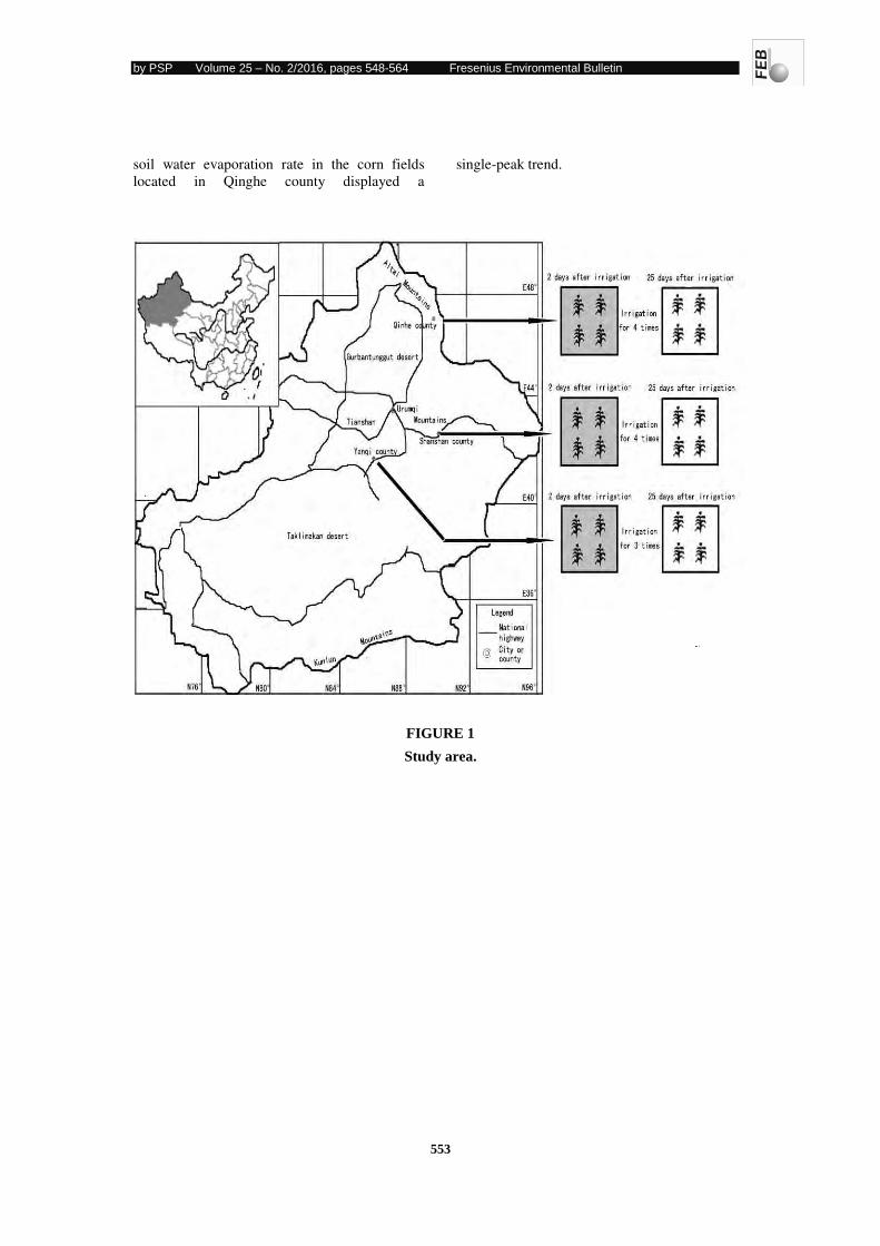
by PSP Volume 25 – No. 2/2016, pages 548-564 Fresenius Environmental Bulletin
553
soil water evaporation rate in the corn fields
located in Qinghe county displayed a
single-peak trend.
FIGURE 1
Study area.
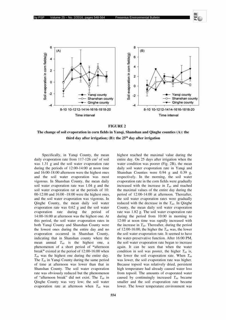
by PSP Volume 25 – No. 2/2016, pages 548-564 Fresenius Environmental Bulletin
554
FIGURE 2
The change of soil evaporation in corn fields in Yanqi, Shanshan and Qinghe counties (A): the
third day after irrigation; (B): the 25th day after irrigation
Specifically, in Yanqi County, the mean
daily evaporation rate from 117-126 cm3 of soil
was 1.31 g and the soil water evaporation rate
during the periods of 12:00-14:00 at noon time
and 16:00-18:00 afternoon were the highest ones
and the soil water evaporation was most
vigorous. In Shanshan County, the mean daily
soil water evaporation rate was 1.04 g and the
soil water evaporation rat at the periods of 10:
00-12:00 and 16:00 -18:00 were the highest ones,
and the soil water evaporation was vigorous. In
Qinghe County, the mean daily soil water
evaporation rate was 0.62 g and the soil water
evaporation rate during the period of
14:00-16:00 at afternoon was the highest one. At
this period, the soil water evaporation rates in
both Yanqi County and Shanshan County were
the lowest ones during the entire day and no
evaporation occurred in Shanshan County,
indicating that in Shanshan county where the
mean annual Tair is the highest one, a
phenomenon of a short period of “afternoon
break” existed at the period of 12:00-16:00 when
Tair was the highest one during the entire day.
The Tair in Yanqi County during the same period
of time at afternoon was lower than that in
Shanshan County. The soil water evaporation
rate was obviously reduced but the phenomenon
of “afternoon break” did not exist. The Tair in
Qinghe County was very low; the soil water
evaporation rate at afternoon when Tair was
highest reached the maximal value during the
entire day. On 25 days after irrigation when the
water condition was poorer (Fig. 2B), the mean
daily soil water evaporation rate in Yanqi and
Shanshan Counties were 0.94 g and 0.39 g,
respectively. In the morning, the soil water
evaporation rate in the corn fields were gradually
increased with the increase in Tair and reached
the maximal values of the entire day during the
period of 12:00-14:00 at afternoon. Thereafter,
the soil water evaporation rates were gradually
reduced with the decrease in the Tair. In Qinghe
County, the mean daily soil water evaporation
rate was 1.82 g. The soil water evaporation rate
during the period from 10:00 in morning to
12:00 at noon time was rapidly increased with
the increase in Tair. Thereafter, during the period
of 12:00-16:00, the higher the Tair was, the lower
the soil water evaporation rate. It seemed to have
the water-preservative function. After 16:00 PM,
the soil water evaporation rate began to increase
again. It can be seen that when the water
condition in soil was poorer, the higher Tair is,
the lower the soil evaporation rate. When Tair
was lower, the soil evaporation rate was higher.
Because topsoil was relatively dried, persistent
high temperature had already caused water loss
from topsoil. The amounts of evaporated water
caused by continuingly increased Tair became
smaller and the soil evaporation rate became
lower. The lower temperature environment was
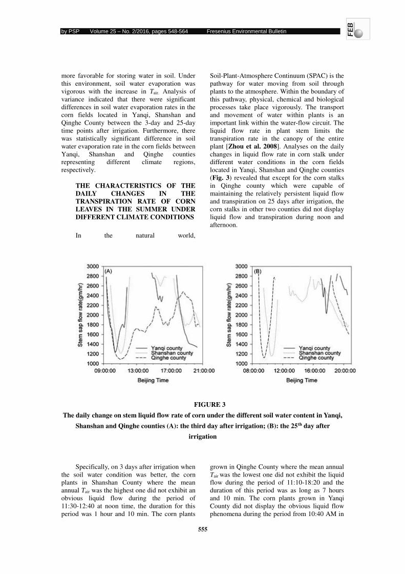
by PSP Volume 25 – No. 2/2016, pages 548-564 Fresenius Environmental Bulletin
555
more favorable for storing water in soil. Under
this environment, soil water evaporation was
vigorous with the increase in Tair. Analysis of
variance indicated that there were significant
differences in soil water evaporation rates in the
corn fields located in Yanqi, Shanshan and
Qinghe County between the 3-day and 25-day
time points after irrigation. Furthermore, there
was statistically significant difference in soil
water evaporation rate in the corn fields between
Yanqi, Shanshan and Qinghe counties
representing different climate regions,
respectively.
THE CHARACTERISTICS OF THE
DAILY CHANGES IN THE
TRANSPIRATION RATE OF CORN
LEAVES IN THE SUMMER UNDER
DIFFERENT CLIMATE CONDITIONS
In the natural world,
Soil-Plant-Atmosphere Continuum (SPAC) is the
pathway for water moving from soil through
plants to the atmosphere. Within the boundary of
this pathway, physical, chemical and biological
processes take place vigorously. The transport
and movement of water within plants is an
important link within the water-flow circuit. The
liquid flow rate in plant stem limits the
transpiration rate in the canopy of the entire
plant [Zhou et al. 2008]. Analyses on the daily
changes in liquid flow rate in corn stalk under
different water conditions in the corn fields
located in Yanqi, Shanshan and Qinghe counties
(Fig. 3) revealed that except for the corn stalks
in Qinghe county which were capable of
maintaining the relatively persistent liquid flow
and transpiration on 25 days after irrigation, the
corn stalks in other two counties did not display
liquid flow and transpiration during noon and
afternoon.
FIGURE 3
The daily change on stem liquid flow rate of corn under the different soil water content in Yanqi,
Shanshan and Qinghe counties (A): the third day after irrigation; (B): the 25th day after
irrigation
Specifically, on 3 days after irrigation when
the soil water condition was better, the corn
plants in Shanshan County where the mean
annual Tair was the highest one did not exhibit an
obvious liquid flow during the period of
11:30-12:40 at noon time, the duration for this
period was 1 hour and 10 min. The corn plants
grown in Qinghe County where the mean annual
Tair was the lowest one did not exhibit the liquid
flow during the period of 11:10-18:20 and the
duration of this period was as long as 7 hours
and 10 min. The corn plants grown in Yanqi
County did not display the obvious liquid flow
phenomena during the period from 10:40 AM in
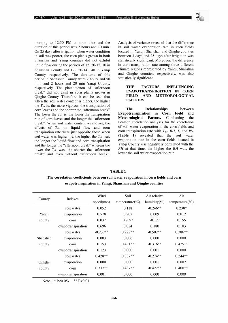
by PSP Volume 25 – No. 2/2016, pages 548-564 Fresenius Environmental Bulletin
556
morning to 12:50 PM at noon time and the
duration of this period was 2 hours and 10 min.
On 25 days after irrigation when water condition
in soil was poorer, the corn plants grown in both
Shanshan and Yanqi counties did not exhibit
liquid flow during the periods of 12 20-15 10 in
Shanshan County and 12 20-14 40 in Yanqi
County, respectively. The durations of this
period in Shanshan County were 2 hours and 50
min, and 2 hours and 20 min Yanqi County,
respectively. The phenomenon of “afternoon break” did not exist in corn plants grown in
Qinghe County. Therefore, it can be seen that
when the soil water content is higher, the higher
the Tair is, the more vigorous the transpiration of
corn leaves and the shorter the “afternoon break”.
The lower the Tair is, the lower the transpiration
rate of corn leaves and the longer the “afternoon break”. When soil water content was lower, the
effects of Tair on liquid flow and corn
transpiration rate were just opposite those when
soil water was higher, i.e. the higher the Tair was,
the longer the liquid flow and corn transpiration
and the longer the “afternoon break” whereas the lower the Tair was, the shorter the “afternoon break” and even without “afternoon break”.
Analysis of variance revealed that the difference
in soil water evaporation rate in corn fields
located in Yanqi, Shanshan and Qinghe counties
between 3 days and 25 days after irrigation was
statistically significant. Moreover, the difference
in corn transpiration rate among three different
climate regions represented by Yanqi, Shanshan
and Qinghe counties, respectively, was also
statistically significant.
THE FACTORS INFLUENCING
EVAPOTRANSPIRATION IN CORN
FIELD AND METEOROLOGICAL
FACTORS
The Relationships between
Evapotranspiration in Corn Field and
Meteorological Factors. Conducting the
Pearson correlation analyses for the correlation
of soil water evaporation in the corn fields and
corn transpiration rate with Tair, RH, Ts and WV
(Table 1) revealed that the soil water
evaporation rate in the corn fields located in
Yanqi County was negatively correlated with the
RH at that time, the higher the RH was, the
lower the soil water evaporation rate.
TABLE 1
The correlation coefficients between soil water evaporation in corn fields and corn
evapotranspiration in Yanqi, Shanshan and Qinghe counties
County Indexes Wind
speed(m/s)
Soil
temperature(℃)
Air relative
humidity(%)
Air
temperature(℃)
Yanqi
county
soil water
evaporation
0.052 0.118 -0.246** 0.238*
0.578 0.207 0.009 0.012
corn
evapotranspiration
0.037 0.209* -0.127 0.155
0.696 0.024 0.180 0.103
Shanshan
county
soil water
evaporation
-0.239** 0.222** -0.502** 0.386**
0.003 0.006 0.000 0.000
corn
evapotranspiration
0.153 0.481** -0.316** 0.425**
0.123 0.000 0.001 0.000
Qinghe
county
soil water
evaporation
0.428** 0.387** -0.274** 0.244**
0.000 0.000 0.001 0.002
corn
evapotranspiration
0.337** 0.487** -0.422** 0.400**
0.001 0.000 0.000 0.000
Note * P<0.05 ** P<0.01
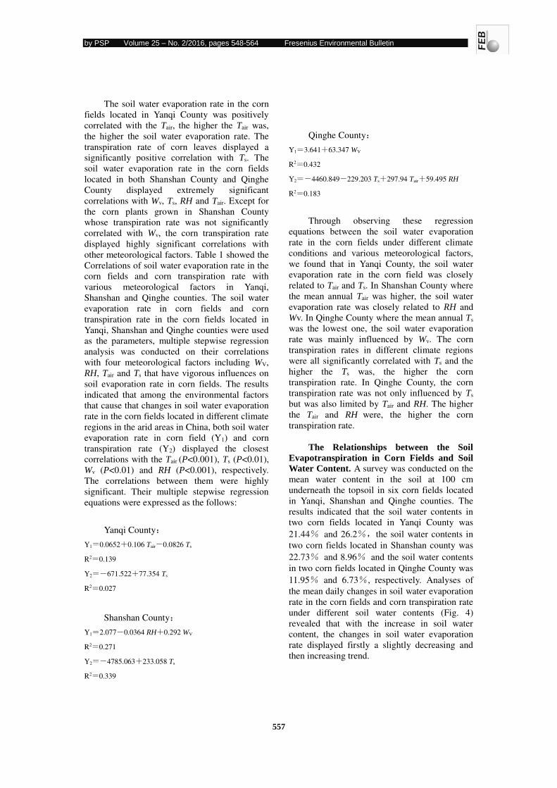
by PSP Volume 25 – No. 2/2016, pages 548-564 Fresenius Environmental Bulletin
557
The soil water evaporation rate in the corn
fields located in Yanqi County was positively
correlated with the Tair, the higher the Tair was,
the higher the soil water evaporation rate. The
transpiration rate of corn leaves displayed a
significantly positive correlation with Ts. The
soil water evaporation rate in the corn fields
located in both Shanshan County and Qinghe
County displayed extremely significant
correlations with Wv, Ts, RH and Tair. Except for
the corn plants grown in Shanshan County
whose transpiration rate was not significantly
correlated with Wv, the corn transpiration rate
displayed highly significant correlations with
other meteorological factors. Table 1 showed the
Correlations of soil water evaporation rate in the
corn fields and corn transpiration rate with
various meteorological factors in Yanqi,
Shanshan and Qinghe counties. The soil water
evaporation rate in corn fields and corn
transpiration rate in the corn fields located in
Yanqi, Shanshan and Qinghe counties were used
as the parameters, multiple stepwise regression
analysis was conducted on their correlations
with four meteorological factors including WV,
RH, Tair and Ts that have vigorous influences on
soil evaporation rate in corn fields. The results
indicated that among the environmental factors
that cause that changes in soil water evaporation
rate in the corn fields located in different climate
regions in the arid areas in China, both soil water
evaporation rate in corn field (Y1) and corn
transpiration rate (Y2) displayed the closest
correlations with the Tair (P<0.001), Ts (P<0.01),
Wv (P<0.01) and RH (P<0.001), respectively.
The correlations between them were highly
significant. Their multiple stepwise regression
equations were expressed as the follows:
Yanqi County
Y1=0.0652 0.106 Tair 0.0826 Ts
R2=0.139
Y2= 671.522 77.354 Ts
R2=0.027
Shanshan County
Y1=2.077 0.0364 RH 0.292 WV
R2=0.271
Y2= 4785.063 233.058 Ts
R2=0.339
Qinghe County
Y1=3.641 63.347 WV
R2=0.432
Y2= 4460.849 229.203 Ts 297.94 Tair 59.495 RH
R2=0.183
Through observing these regression
equations between the soil water evaporation
rate in the corn fields under different climate
conditions and various meteorological factors,
we found that in Yanqi County, the soil water
evaporation rate in the corn field was closely
related to Tair and Ts. In Shanshan County where
the mean annual Tair was higher, the soil water
evaporation rate was closely related to RH and
Wv. In Qinghe County where the mean annual Ts
was the lowest one, the soil water evaporation
rate was mainly influenced by Wv. The corn
transpiration rates in different climate regions
were all significantly correlated with Ts and the
higher the Ts was, the higher the corn
transpiration rate. In Qinghe County, the corn
transpiration rate was not only influenced by Ts
but was also limited by Tair and RH. The higher
the Tair and RH were, the higher the corn
transpiration rate.
The Relationships between the Soil
Evapotranspiration in Corn Fields and Soil
Water Content. A survey was conducted on the
mean water content in the soil at 100 cm
underneath the topsoil in six corn fields located
in Yanqi, Shanshan and Qinghe counties. The
results indicated that the soil water contents in
two corn fields located in Yanqi County was
21.44% and 26.2% the soil water contents in
two corn fields located in Shanshan county was
22.73% and 8.96% and the soil water contents
in two corn fields located in Qinghe County was
11.95% and 6.73%, respectively. Analyses of
the mean daily changes in soil water evaporation
rate in the corn fields and corn transpiration rate
under different soil water contents (Fig. 4)
revealed that with the increase in soil water
content, the changes in soil water evaporation
rate displayed firstly a slightly decreasing and
then increasing trend.
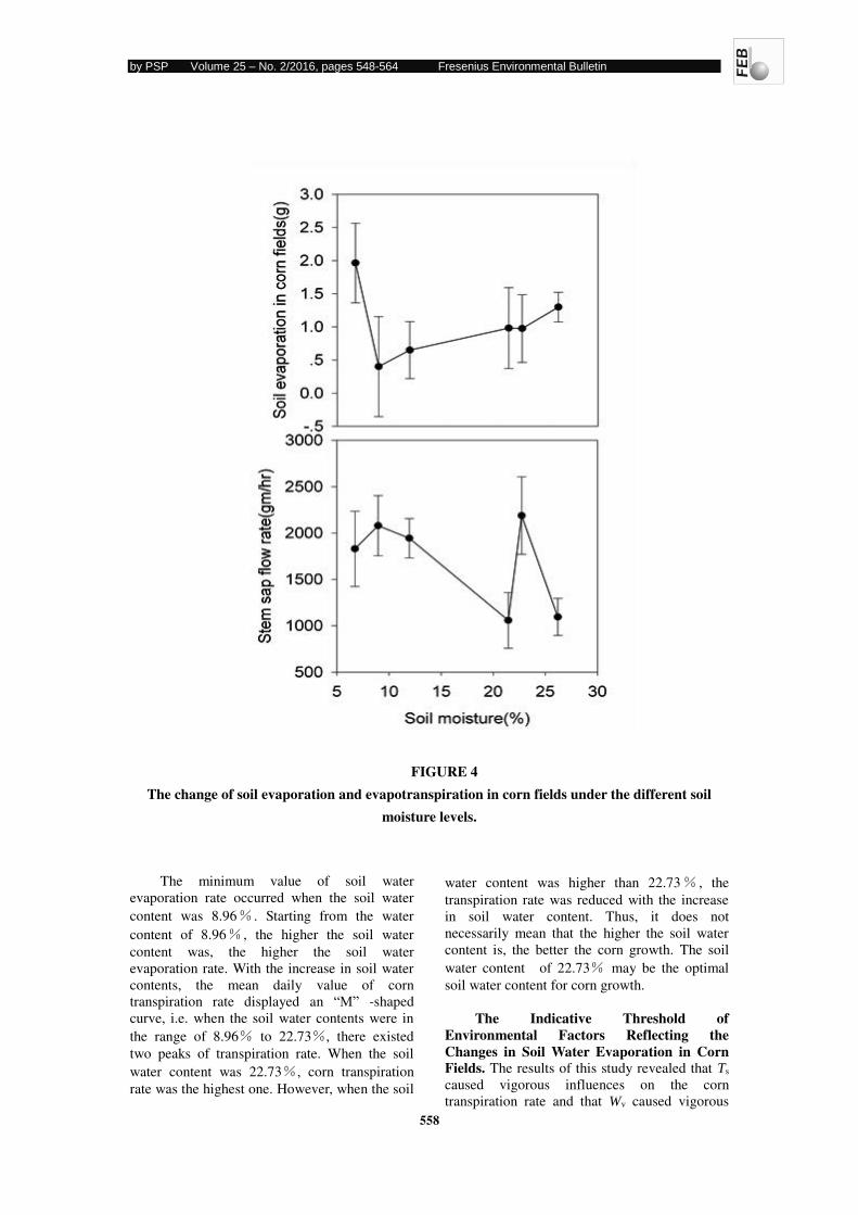
by PSP Volume 25 – No. 2/2016, pages 548-564 Fresenius Environmental Bulletin
558
FIGURE 4
The change of soil evaporation and evapotranspiration in corn fields under the different soil
moisture levels.
The minimum value of soil water
evaporation rate occurred when the soil water
content was 8.96% . Starting from the water
content of 8.96% , the higher the soil water
content was, the higher the soil water
evaporation rate. With the increase in soil water
contents, the mean daily value of corn
transpiration rate displayed an “M” -shaped
curve, i.e. when the soil water contents were in
the range of 8.96% to 22.73%, there existed
two peaks of transpiration rate. When the soil
water content was 22.73%, corn transpiration
rate was the highest one. However, when the soil
water content was higher than 22.73% , the
transpiration rate was reduced with the increase
in soil water content. Thus, it does not
necessarily mean that the higher the soil water
content is, the better the corn growth. The soil
water content of 22.73% may be the optimal
soil water content for corn growth.
The Indicative Threshold of
Environmental Factors Reflecting the
Changes in Soil Water Evaporation in Corn
Fields. The results of this study revealed that Ts
caused vigorous influences on the corn
transpiration rate and that Wv caused vigorous
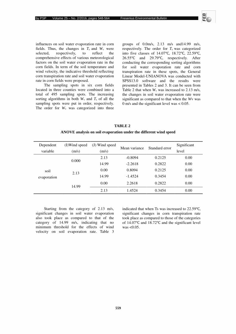
by PSP Volume 25 – No. 2/2016, pages 548-564 Fresenius Environmental Bulletin
559
influences on soil water evaporation rate in corn
fields. Thus, the changes in Ts and Wv were
selected, respectively, to reflect the
comprehensive effects of various meteorological
factors on the soil water evaporation rate in the
corn fields. In term of the soil temperature and
wind velocity, the indicative threshold reflecting
corn transpiration rate and soil water evaporation
rate in corn fields were proposed.
The sampling spots in six corn fields
located in three counties were combined into a
total of 495 sampling spots. The increasing
sorting algorithms in both Wv and Ts of all the
sampling spots were put in order, respectively.
The order for Wv was categorized into three
groups of 0.0m/s, 2.13 m/s and14.99 m/s,
respectively. The order for Ts was categorized
into five classes of 14.07℃, 18.72℃, 22.59℃,
26.55℃ and 29.79℃, respectively. After
conducting the corresponding sorting algorithms
for soil water evaporation rate and corn
transpiration rate in these spots, the General
Linear Model-UNIANOVA was conducted with
SPSS13.0 software and the results were
presented in Tables 2 and 3. It can be seen from
Table 2 that when Wv was increased to 2.13 m/s,
the changes in soil water evaporation rate were
significant as compared to that when the Wv was
0 m/s and the significant level was < 0.05.
TABLE 2
ANOVE analysis on soil evaporation under the different wind speed
Dependent
variable
(I)Wind speed
(m/s)
(J) Wind speed
(m/s) Mean variance Standard error
Significant
level
soil
evaporation
0.000 2.13 -0.8094 0.2125 0.00
14.99 -2.2618 0.2822 0.00
2.13 0.00 0.8094 0.2125 0.00
14.99 -1.4524 0.3454 0.00
14.99 0.00 2.2618 0.2822 0.00
2.13 1.4524 0.3454 0.00
Starting from the category of 2.13 m/s,
significant changes in soil water evaporation
also took place as compared to that of the
category of 14.99 m/s, indicating that no
minimum threshold for the effects of wind
velocity on soil evaporation rate. Table 3
indicated that when Ts was increased to 22.59℃,
significant changes in corn transpiration rate
took place as compared to those of the categories
of 14.07℃ and 18.72℃ and the significant level
was <0.05.
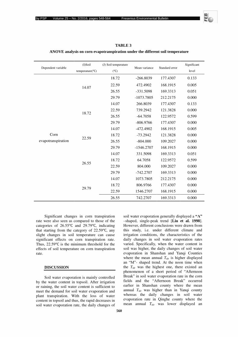
by PSP Volume 25 – No. 2/2016, pages 548-564 Fresenius Environmental Bulletin
560
TABLE 3
ANOVE analysis on corn evapotranspiration under the different soil temperature
Dependent variable (I)Soil
temperature(℃)
(J) Soil temperature
(℃) Mean variance Standard error
Significant
level
Corn
evapotranspiration
14.07
18.72 -266.8039 177.4307 0.133
22.59 472.4902 168.1915 0.005
26.55 -331.5098 169.3313 0.051
29.79 -1073.7805 212.2175 0.000
18.72
14.07 266.8039 177.4307 0.133
22.59 739.2942 121.3828 0.000
26.55 -64.7058 122.9572 0.599
29.79 -806.9766 177.4307 0.000
22.59
14.07 -472.4902 168.1915 0.005
18.72 -73.2942 121.3828 0.000
26.55 -804.000 109.2027 0.000
29.79 -1546.2707 168.1915 0.000
26.55
14.07 331.5098 169.3313 0.051
18.72 64.7058 122.9572 0.599
22.59 804.000 109.2027 0.000
29.79 -742.2707 169.3313 0.000
29.79
14.07 1073.7805 212.2175 0.000
18.72 806.9766 177.4307 0.000
22.59 1546.2707 168.1915 0.000
26.55 742.2707 169.3313 0.000
Significant changes in corn transpiration
rate were also seen as compared to those of the
categories of 26.55℃ and 29.79℃, indicating
that starting from the category of 22.59℃, any
slight changes in soil temperature can cause
significant effects on corn transpiration rate.
Thus, 22.59℃ is the minimum threshold for the
effects of soil temperature on corn transpiration
rate.
DISCUSSION
Soil water evaporation is mainly controlled
by the water content in topsoil. After irrigation
or raining, the soil water content is sufficient to
meet the demand for soil water evaporation and
plant transpiration. With the loss of water
content in topsoil and thus, the rapid decreases in
soil water evaporation rate, the daily changes of
soil water evaporation generally displayed a “Λ”
–shaped, single-peak trend [Liu et al. 1998].
However, different conclusions were drawn from
this study, i.e. under different climate and
irrigation conditions, the characteristics of the
daily changes in soil water evaporation rates
varied. Specifically, when the water content in
soil was higher, the daily changes of soil water
evaporation in Shanshan and Yanqi Counties
where the mean annual Tair is higher displayed
an “M”- shaped trend. At the noon time when
the Tair was the highest one, there existed an
phenomenon of a short period of “Afternoon Break” in soil water evaporation rate in the corn
fields and the “Afternoon Break” occurred earlier in Shanshan county where the mean
annual Tair was higher than in Yanqi county
whereas the daily changes in soil water
evaporation rate in Qinghe county where the
mean annual Tair was lower displayed an
by PSP Volume 25 – No. 2/2016, pages 548-564 Fresenius Environmental Bulletin
561
“Λ”-shaped trend and no “Afternoon Break” existed. This is due to the reason that under the
high temperature condition, the water adhered to
topsoil is rapidly evaporated and with the
continuing increase in temperature, the
evaporable water adhered in soil surface become
lower or is zero, thus, under the high
temperature condition, the soil water evaporation
rate is reduced or is zero and displayed an
“Afternoon Break”. In the afternoon, with the
decrease in Tair, the water content in the deeper
soil layers is moved up through capillary and
reaches the shallow layer underneath the topsoil.
At this time, there is higher amount of water
adhered to topsoil that can be used for
evaporation, thus, under the action of
transpiration driving force, the soil water
evaporation rate starts to increase. High
temperature can rapidly evaporate the water in
the topsoil. When the water content in the deeper
soil layers is lower and cannot provide the
supplement of water for topsoil in time, the
water requirement for the corn growth at
afternoon can be affected whereas the low
temperature is favorable for water storage in soil
and the corn growth at afternoon is not affected.
When soil water content is lower and the
mean soil water evaporation rate is also lower,
the daily changes in soil water evaporation rate
in Yanqi and Shanshan counties displayed a
“W”-shaped trend, and no “Afternoon Break” existed. This is due to the reason that the topsoil
is drier. The mean soil water evaporation rate in
Yanqi and Shanshan counties was only 0.62 g,
which was far lower than the soil water
evaporation rate of 1.17 g when the soil water
condition was good. When Tair is increased, the
small amount of water in the soil is gradually
evaporated on the basis of the lower soil water
evaporation rate. In afternoon, with the decrease
in Tair, the lower amount of water in the deeper
layers of soil is unable to supplement the topsoil
in time and thus, the soil water evaporation rate
became lower and lower. After the period of
16:00-18:00 PM, the soil water evaporation rate
started to increase again. In Qinghe County,
because the Tair is always lower there, thus, even
on 25 days after irrigation, the status of soil
water content was still quite good, with the
increase in Tair, the soil water evaporation rate
reached the maximal value during the period of
10:00-12:00 at noon time. In afternoon, the soil
water evaporation rate was slightly reduced and
started to increase again at the period of
14:00-16:00 PM. This is due to the reason that
even the water in the shallow layers of topsoil is
completely evaporated under the high
temperature condition, water in the deeper soil
layers can supplement in time to the topsoil. This
similarly indicates that low temperature is
favorable for corn growth under the environment
of lower soil water content.
Analyses on the characteristics of the daily
changes in transpiration rate of corn leaves under
different Tair and irrigation conditions revealed
that on 3 days after irrigation when the soil water
content was higher, the phenomenon of liquid
flow and corn transpiration did not occur at noon
time, i.e. there existed the phenomenon of
“Afternoon Break”. Specifically, the no-liquid
flow existed in the period of 11:30-12:40 at noon
time in Shanshan County where the mean annual
Tair is higher and the duration of no-liquid flow
was 1 hour and 10 min. The no-liquid flow
occurred during the period of 11:10-18:20 in
Qinghe County where the mean annual
temperature is lower and the duration of
no-liquid flow was as long as 7 hours and 10
min. The no-liquid flow occurred during the
period of 10:40-12:50 at noon time in Yanqi
County where the mean annual Tair is between
those of Shanshan county and Qinghe county.
The duration of no-liquid flow was 2 hours and
10 min. It can be seen that the higher the Tair is,
the shorter the “Afternoon Break” and is more
favorable for corn growth. The lower Tair is, the
longer the “Afternoon Break” and is less
favorable for corn growth. On 25 days after
irrigation when the soil water content was lower,
the phenomenon of no-liquid flow and
transpiration existed in corn leaves in both
Shanshan and Yanqi counties where the mean
annual Tair is higher, among which no-liquid
flow occurred during the period of 12:20-15:10
in Shanshan county where Tair is higher and the
duration of No-liquid flow was 2 hours and 50
min. The no-liquid flow occurred during the
period of 12:20-14:40 in Yanqi County where
the Tair is lower and the duration of no-liquid
flow was 2 hours and 20 min. The no-liquid flow
did not exist in corn leaves in Qinghe county
where the Tair is lowest, indicating that when soil
water content is lower, the higher the Tair is, the
longer the “Afternoon Break” and the less
favorable for corn growth; the lower the Tair is,
the shorter the Afternoon Break” or even no
“Afternoon Break” occurred, and is more
favorable for corn growth. Thus, it can be
inferred that when soil is deficient in water,
lower temperature is favorable for corn growth
and when the soils have sufficient water, higher
temperature is favorable for corn growth. When
corn is growing under a low temperature
environment, the frequencies of irrigation can be
by PSP Volume 25 – No. 2/2016, pages 548-564 Fresenius Environmental Bulletin
562
properly reduced whereas when corn is growing
under a high temperature environment, the
frequencies of irrigation can be properly
increased.
A large number of studies have been
conducted on how to reduce soil water
evaporation and how to increase the water use
efficiency of crops, including the drip irrigation
measure, coverage cultivation, increase in leaf
area index at the earlier stage of crop growth and
reduction of the water content in topsoil under
the crown layer to control the non-production
consumption of water in fields [Liu et al. 1998].
Zero-tillage can effectively reduce soil water
evaporation rate and increase the transpiration
consumption of water [Zhang et al. 2003].
Covering the soil with ground sheeting can
largely reduce the soil water evaporation rate
[Meng et al. 2003]. The high stubble harvesting
of wheat grains was an effective way to increase
the water use efficiency in row-intercropping of
corn with wheat in the oasis irrigated areas
[Kang and cai 1996; Jing et al., 2010]. Larger
irrigation norm and fewer irrigation frequencies
can reduce the soil water evaporation rate in
winter wheat fields and increased the irrigated
water use efficiency [Yu et al. 2009]. The study
by Yuan et al. observed that gravel-derived
coverage materials had larger effects on topsoil
water evaporation rate in arid and semi-arid
regions [Yuan et al. 2009]. In the arid regions
located in northwest of China, through
quantitative interpretation of the impacts of the
meteorological factors and soil water contents on
the changes in soil water evaporation in corn
fields will allow us to find out the characteristics
of the living environment indicative the changes
in soil water evaporation rate in corn fields. In
this study, we found that the soil water
evaporation rate in corn field had significant
correlations with Tair, Wv, Ts and RH and that
corn transpiration rate had significant
correlations with Ts, RH and Tair. If we need to
reduce the soil water evaporation in the corn
fields, we need to implement the appropriate
measures and/or treatments to reduce the
temperature and Wv and to increase the Ts and
RH in the fields where corn is grown. For these
measures, two rows of crops with higher height
such as sorghum and sunflowers can be planted
in the outside boundary of the corn fields to
reduce the Wv and to prevent the leakage of
water vapor from the corn field environment and
thus, maintain higher RH in corn fields. In
general, after the treatments for increasing Ts and
RH have been implemented, the soil water
evaporation in the corn fields can be effectively
reduced and thus, the corn transpiration rate can
be increased. Because 22.59℃ is the minimum
threshold for soil temperature that affects corn
transpiration rate, after the biological measures
have been implemented, the soil temperature
needs to be maintained at above 22.59℃.
Additionally, this study also found that when the
soil water content was 22.73 % , corn
transpiration rate was the highest one. When soil
water content was above the 22.73% , corn
transpiration rate was reduced with the increase
in soil water contents. Thus, it can be inferred
that the soil water content of 22.73% may be
the optimal soil water content for corn growth.
The soil water content can be maintained at
about 22.73% through controlling the irrigation
frequencies and the irrigation norm.
ACKNOWLEDGEMENTS
This study was supported financially by
National Natural Science Foundation of China
(Grant No. 41271052, 41561023), Foundation of
State Key Laboratory of Desert and Oasis
Ecology (Y471166), the project of autonomous
scientific and technological youth personnel
training (2013731025).
REFERENCES
[1] M. Aydin, S.L. Yang, N. Kurt, et al. Test of
a simple model for estimating evaporation
from bare soils in different environments.
Ecological Modelling, 2005,182(1):
91-105.
[2] M. Bittelli, F. Ventura, G.S. Campbell, et al.
Coupling of heat, water vapor and liquid
water fluxes to compute evaporation in
bare soils. Journal of Hydrology, 2008,
362(3-4):191-205.
[3] Q. Chai, A.Z. Yu, G.P. Chen, et al. Soil
evaporation under sole cropping and
intercropping systems and the main driving
factors.Chinese Journal of Eco-Agriculture,
2011,19(6):1307-1312.
[4] G. Alvenas, P.E. Jansson. Model for
evaporation, moisture and temperature of
bare soil: calibration and sensitivity
analysis. Agricultural and Forest
Meteorology, 1997,88(1-4): 47-56.
[5] M. Jing, B.Z Jiang, H.M. Zhang, et al.
Effect of different mulching materials to
soil evaporation of spring wheat in arid
region. Journal of Water Resources and
by PSP Volume 25 – No. 2/2016, pages 548-564 Fresenius Environmental Bulletin
563
Water Engineering, 2010,21(2):92-95.
[6] S.Z. Kang, H.J. Cai. Agricultural water
management. Beijing: china agriculture
press. 1996.
[7] B.L. Kerridge, J.W. Hornbuckle, E.W.
Christen, et al. Using soil surface
temperature to assess soil evaporation in a
drip irrigated vineyard. Agricultural Water
Management, 2013, 116: 128-141.
[8] W.Q. Liang, H.J. Cai, J. Wang. Research of
evapotranspiration and evaporation for
winter wheat. Journal of Irrigation and
Drainage, 2011,30(6):93-96.
[9] C.M. Liu, X.Y. Zhang, Y.Q. Zhang
Determination of daily evaporation and
evapotranspiration of winter wheat field by
large-scale weighing lysimeter and micro
lysimeter. Agricultural and Forest
Meteorology, 2002,111(2):109-120.
[10] S.M. Ma, E.D. Lin, S.S. Ma. The influence
of climate change on agriculture and
Countermeasures -- climate change and
agriculture, rural development and
livelihood of farmers. Science Chinese,
2011,5: 18-23.
[11] Q. Meng, Y. Li, G.P. Feng. Effects of plastic
film mulch Patterns on soil surface
evaporation. Irrigation and Drainage,
2003,22(2):17-20.
[12] G.P. Mengu, S. Anac, K. Topcuoglu
Analysis of drought in the Marmara region
using the Standardized Precipitation Index.
Fresenius Environmental Bulletin,
2009,18(5):633-641.
[13] G. P. Mengu, E. Akkuzu, S. Anac, et al.
Impact of climate change on irrigated
agriculture. Fresenius Environmental
Bulletin, 2011,20(3A):823-830.
[14] G.Y. Qiu, P.J. Shi, L.M. Wang. Theoretical
analysis of a remotely measurable soil
evaporation transfer coefficient. Remote
sensing of environment, 2006,
101(3):390-398.
[15] H. Blanco-Canqui, R. Lal Climate change
and soil erosion risks. Principles of Soil
Conservation and Management, 2008,
513-536.
[16] J. Southworth, P.A. Pfeifer, M. Habeck, et
al. Sensitivity of winter wheat yields in the
Mid-western United States to future
changes in climate, climate variability, and
CO2 fertilization. Climatic change, 2002,
22(1): 73-86.
[17] T.C. Baruah, S. Hasegawa. In-situ
measurement of soil evaporation from a
volcanic ash soil by TDR technique using
soil water diffusivity. Geodema,
2001,102(3-4):317-328.
[18] W.H. Terjung, D.M. Liverman, J.T. Hayes,
Climatic change and water requirements
for grain corn in the North American great
plains. Climatic change,
1984,6(2):193-220.
[19] A.Usta, M.Yilmaz, S. Malkocoglu, et al.
Effects of environmental factors on wood
anatomy of black alder (Alnus glutinosa (L.)
Gaertner subsp barbata (CA Meyer) Yalt)
from two different origins of eastern black
sea region in Turkey. Fresenius
Environmental Bulletin,
2014,23(8):1778-1784.
[20] J.S.Wallace, N.A.Jackson, C.K.Ong.
Modelling soil evaporation in an
agroforestry system in Kenya. Agricultural
and Forest Meteorology,
1999,94(3-4):189-202
[21] .J. Wang, H.J. Cai, F. Chen, et al.
Experimental study on evapotranspiration
and soil evaporation in summer maize field.
Journal of Water Resources and Water
Engineering, 2004,11:108-113.
[22] T. Yamanaka, T. Yonetani. Dynamics of the
evaporation zone in dry sandy soils.
Journal of Hydrology, 1999,217(1-2):
135-148.
[23] L.P. Yu, G.H. Huang, H.J. Liu, et al.
Experimental investigation of soil
evaporation and evapotranspiration of
winter wheat under sprinkler irrigation.
Agricultural Sciences in China, 2009, 8(11):
1360-1368.
[24] C.P. Yuan, T.W. Lei, L.L. Mao, et al. Soil
surface evaporation processes under
mulches of different sized gravel. Catena,
2009,78(2):117-121.
[25] H.L. Zhang, Y.D. Qin, W.S. Zhu. Study on
soil evaporation of no-tillage with mulch.
Chinese Journal of Soil Science,
2003,34(4):259-261.
[26] P. Zhou. The possible influence of global
climate changes on agricultural production
in China and counter measures. Journal of
Yunnan Agricultural University,
2001,16(1):1-4.
[27] X.M. Zhou, Y.N. Chen, W.H. Li, et al.
Study of sap flow in stem of Populus
euphratica in the lower reaches of Tarim
River. Journal of Desert Research,
2008,28(4):673-678.
Received: 21.07.2015
Accepted: 05.12.2015

by PSP Volume 25 – No. 2/2016, pages 548-564 Fresenius Environmental Bulletin
564
CORRESPONDING AUTHOR
Aihong Fu
Chinese Academy of Sciences
Xinjiang Institute of Ecology and Geography
State Key Laboratory of Desert and Oasis
Ecology
818 South Beijing Road
Urumqi 830011 – CHINA
e-mail: [email protected]
by PSP Volume 25 – No. 2/2016, pages 565-579 Fresenius Environmental Bulletin
565
SHORT AND LONG TERM STREAMFLOW PREDICTION BY DIFFERENT NEURAL NETWORK APPROACHES AND TREND
ANALYSIS METHODS: CASE STUDY OF SAKARYA RIVER, TURKEY
Osman Sonmez1, Gokmen Ceribasi2, Emrah Dogan1
1Sakarya University, Faculty of Engineering, Department of Civil Engineering, Sakarya, Turkey
2Sakarya University, Technology Faculty, Department
ABSTRACT
The estimation of flow is required for planning and
operating many hydraulic structure in rivers. This study
presents the application of Artificial Neural Networks
(ANNs) and trend analysis methods in predicting short
and long term streamflows. Estimations was made by
using flow datas of Sakarya River, Turkey between 1989
and 2000. In ANN models were based on the daily
streamflow data for predicting short term streamflows
although trend analysis methods were based on the
monthly streamflow data for predicating long term
streamflows. The flow data of 4.018 days were used as
training and testing sets for the chosen all ANN models in
this study. Among these, 2.650 days (approximately %65
of all data) were reserved for the calibration/training set
and the remaining data (approximately %35 of all data)
were used for the validation/testing set. For predicting
flow of Sakarya Rivers, seven different scenarios were
analyzed for four different ANN models and three
different trend analysis method. The performance criteria
of the neural network is depend of Mean Absolute Error
(MAE), Nash-Sutcliffe Sufficiency Score (NSSS) and
coefficient of correlation (R-value) parameters. The
results were compared with each other for determine the
best approaches. For long term streamflow prediction,
The Mann-Kendall test and Spearman Rho test were used
in the study. The Mann-Kendall Rank Correlation test
was used to determine the trend’s starting year. In the
result of these analysis shows that Feed Forward Neural
Networks (FFNN) gave the best results, with respect to
performance criteria for short term prediction. In addition,
downward trends in test statistics of Sakarya River also
indicate that water will decrease in next years. Thus, to
leave healthy and adequate amount of water to the next
generations, Turkey should preserve and rationally use its
sources.
KEYWORDS: Streamflow, Artificial Neural Networks, Trend Analysis,
Sakarya River
INTRODUCTION
Water is one of the essentials for the existence and
continuance of life. Water is one of the most important
natural resources which are indispensable for humans and
all organisms. Furthermore, Water is essential for nearly
all sectors, such as industry, agriculture, energy,
environment and usage within ecosystems and national
security.
The Artificial Neural Networks (ANNs) are
intelligent computation computer techniques, which are
inspired by studies on the human brain. ANN approaches
have been successfully applied in a number of diverse
fields, including water resources. ANNs can learn from
training patterns and respond successfully to unknown
situations. In the hydrological context, recent experiments
have reported that ANNs may offer a promising
alternative for evapotranspiration modeling [1-4], rainfall-
runoff modeling [5, 6], streamflow prediction [7-10],
reservoir inflow forecasting [11, 12], and suspended
sediment estimation [13, 14]. The results indicate that the
proposed model could significantly increase the short and
long-term forecast accuracy [15].
On the other hand, Climatic conditions are among
the most changeable conditions in the earth. Today water
resources are threatened by climate change [5]. Since
water’s characteristics change over time, it always shows
a tendency to increase or decrease. For this reason, certain
methods are used to make estimations using available
data. The Trend Analysis method, whose reliability has
been proven by many studies, is among these methods. It
is quite important to make comparison between these
methods since both of them make prospective long and
short-term estimation with available data. Because these
two methods are being used in most of the studies that
have been carried out in recent years. Therefore, in this
study, was aimed to long and short-term streamflow
prediction using Trend Analysis Method and Artificial
Neural Networks Method on Sakarya River.
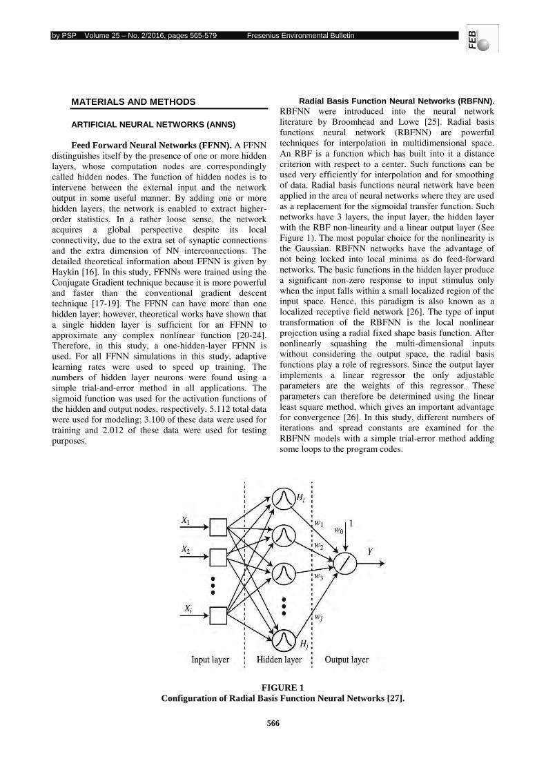
by PSP Volume 25 – No. 2/2016, pages 565-579 Fresenius Environmental Bulletin
566
MATERIALS AND METHODS
ARTIFICIAL NEURAL NETWORKS (ANNS)
Feed Forward Neural Networks (FFNN). A FFNN
distinguishes itself by the presence of one or more hidden
layers, whose computation nodes are correspondingly
called hidden nodes. The function of hidden nodes is to
intervene between the external input and the network
output in some useful manner. By adding one or more
hidden layers, the network is enabled to extract higher-
order statistics. In a rather loose sense, the network
acquires a global perspective despite its local
connectivity, due to the extra set of synaptic connections
and the extra dimension of NN interconnections. The
detailed theoretical information about FFNN is given by
Haykin [16]. In this study, FFNNs were trained using the
Conjugate Gradient technique because it is more powerful
and faster than the conventional gradient descent
technique [17-19]. The FFNN can have more than one
hidden layer; however, theoretical works have shown that
a single hidden layer is sufficient for an FFNN to
approximate any complex nonlinear function [20-24].
Therefore, in this study, a one-hidden-layer FFNN is
used. For all FFNN simulations in this study, adaptive
learning rates were used to speed up training. The
numbers of hidden layer neurons were found using a
simple trial-and-error method in all applications. The
sigmoid function was used for the activation functions of
the hidden and output nodes, respectively. 5.112 total data
were used for modeling; 3.100 of these data were used for
training and 2.012 of these data were used for testing
purposes.
Radial Basis Function Neural Networks (RBFNN).
RBFNN were introduced into the neural network
literature by Broomhead and Lowe [25]. Radial basis
functions neural network (RBFNN) are powerful
techniques for interpolation in multidimensional space.
An RBF is a function which has built into it a distance
criterion with respect to a center. Such functions can be
used very efficiently for interpolation and for smoothing
of data. Radial basis functions neural network have been
applied in the area of neural networks where they are used
as a replacement for the sigmoidal transfer function. Such
networks have 3 layers, the input layer, the hidden layer
with the RBF non-linearity and a linear output layer (See
Figure 1). The most popular choice for the nonlinearity is
the Gaussian. RBFNN networks have the advantage of
not being locked into local minima as do feed-forward
networks. The basic functions in the hidden layer produce
a significant non-zero response to input stimulus only
when the input falls within a small localized region of the
input space. Hence, this paradigm is also known as a
localized receptive field network [26]. The type of input
transformation of the RBFNN is the local nonlinear
projection using a radial fixed shape basis function. After
nonlinearly squashing the multi-dimensional inputs
without considering the output space, the radial basis
functions play a role of regressors. Since the output layer
implements a linear regressor the only adjustable
parameters are the weights of this regressor. These
parameters can therefore be determined using the linear
least square method, which gives an important advantage
for convergence [26]. In this study, different numbers of
iterations and spread constants are examined for the
RBFNN models with a simple trial-error method adding
some loops to the program codes.
FIGURE 1
Configuration of Radial Basis Function Neural Networks [27].
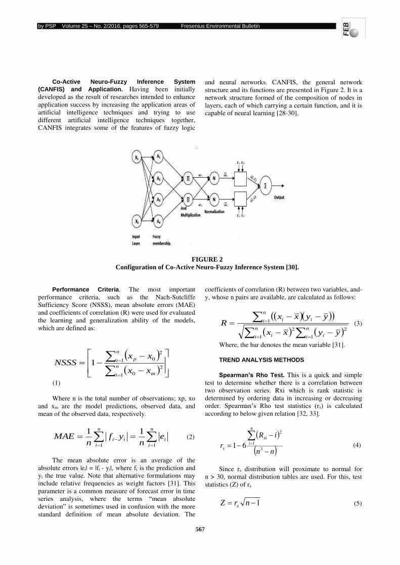
by PSP Volume 25 – No. 2/2016, pages 565-579 Fresenius Environmental Bulletin
567
Co-Active Neuro-Fuzzy Inference System
(CANFIS) and Application. Having been initially
developed as the result of researches intended to enhance
application success by increasing the application areas of
artificial intelligence techniques and trying to use
different artificial intelligence techniques together,
CANFIS integrates some of the features of fuzzy logic
and neural networks. CANFIS, the general network
structure and its functions are presented in Figure 2. It is a
network structure formed of the composition of nodes in
layers, each of which carrying a certain function, and it is
capable of neural learning [28-30].
FIGURE 2
Configuration of Co-Active Neuro-Fuzzy Inference System [30].
Performance Criteria. The most important
performance criteria, such as the Nach-Sutcliffe
Sufficiency Score (NSSS), mean absolute errors (MAE)
and coefficients of correlation (R) were used for evaluated
the learning and generalization ability of the models,
which are defined as:
n
i m
n
i p
xx
xxNSSS
1
2
0
1
2
01
(1)
Where n is the total number of observations; xp, xo
and xm are the model predictions, observed data, and
mean of the observed data, respectively.
n
i
i
n
i
ii en
yfn
MAE11
11 (2)
The mean absolute error is an average of the
absolute errors |ei| = |fi - yi|, where fi is the prediction and
yi the true value. Note that alternative formulations may
include relative frequencies as weight factors [31]. This
parameter is a common measure of forecast error in time
series analysis, where the terms “mean absolute
deviation” is sometimes used in confusion with the more
standard definition of mean absolute deviation. The
coefficients of correlation (R) between two variables, and-
y, whose n pairs are available, are calculated as follows:
n
i
n
i ii
n
i ii
yyxx
yyxxR
1 1
22
1 (3)
Where, the bar denotes the mean variable [31].
TREND ANALYSIS METHODS
Spearman’s Rho Test. This is a quick and simple
test to determine whether there is a correlation between
two observation series. Rxi which is rank statistic is
determined by ordering data in increasing or decreasing
order. Spearman’s Rho test statistics (rs) is calculated
according to below given relation [32, 33].
nn
iR
r
n
i
xi
s
3
1
2
61 (4)
Since rs distribution will proximate to normal for
n > 30, normal distribution tables are used. For this, test
statistics (Z) of rs
1 nrZ s (5)
by PSP Volume 25 – No. 2/2016, pages 565-579 Fresenius Environmental Bulletin
568
It is concluded that if normal distribution
corresponding to significance level which is chosen as
absolute value of Z is smaller than Z/2 then null
hypothesis is accepted and it is concluded that there is no
trend in time series observed; if it is bigger it is concluded
that there is trend and Z value is positive there is increase
trend and if it is negative there is decrease trend [32, 33].
Mann-Kendall Test. Since the Mann-Kendall test is
a non-parametric test, it is independent from distribution
of random variable. With this test, the presence of a trend
in a time series is checked with null hypothesis “H0: no
trend” [34-41]. In x1, x2, ........., xn time series on which
the test will be applied xi, xj pairs are divided into two
groups. For i < j, if the number of the pairs xi < xj is
indicated with P and number of the pairs xi > xj test
statistics (S) is calculated by the following relation:
MPS (6)
Kendall correlation coefficient:
2/1
nn
S (7)
For n ≥ 10
18/521 nnns (8)
0
0
0
/)1(
0
/)1(
S
S
S
S
S
Z
s
s
(9)
It is concluded that if normal distribution
corresponding to significance level which is chosen as
absolute value of Z is smaller than Z/2 then null
hypothesis is accepted and it is concluded that there is no
trend in time series observed; if it is bigger it is concluded
that there is trend and iv Z value is positive there is
increase trend and if it is negative there is decrease trend
[42-44].
Mann-Kendall Rank Correlation test. This
nonparametric test is used to determine whether an
increase or decrease is present in the applied series in
time. The test graphically expresses the results and also
determines starting point of the trend [33]. In
hydrometeorology time series, considering data one by
one from the left, the number of data among the ones
previous than the data are counted. If this number is
called ni then xi data values are replaced with them and a
whole number sample function is obtained. If sequential
sums of these whole numbers are indicated with ti, (t)
which the magnitude required to test the method becomes:
n
i
int1
(10)
Mean E(t) is a follows:
4
1
nntE (11)
Variance is a follows:
72
521var
nnnt (12)
u(t) function is a follows:
t
tEttu
var
(13)
While the assumption, that there is no change over
time, is expressed by the near-zero values of u(t), the
bigger values of u(t) show that a change occurs. On the
other hand, graphical intersection point of u(t) and u’(t) shows the starting time of the trend. As an example,
Figure 3 shows u(t) - u’(t) graph in the case of an existing trend and Figure 4 shows u(t) - u’(t) graph when there is no trend [33, 42-44].
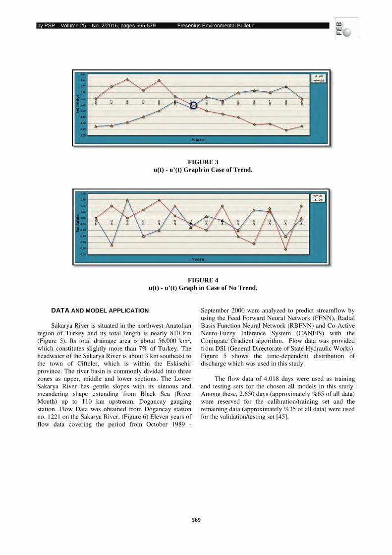
by PSP Volume 25 – No. 2/2016, pages 565-579 Fresenius Environmental Bulletin
569
FIGURE 3
u(t) - u’(t) Graph in Case of Trend.
FIGURE 4
u(t) - u’(t) Graph in Case of No Trend.
DATA AND MODEL APPLICATION
Sakarya River is situated in the northwest Anatolian
region of Turkey and its total length is nearly 810 km
(Figure 5). Its total drainage area is about 56.000 km2,
which constitutes slightly more than 7% of Turkey. The
headwater of the Sakarya River is about 3 km southeast to
the town of Cifteler, which is within the Eskisehir
province. The river basin is commonly divided into three
zones as upper, middle and lower sections. The Lower
Sakarya River has gentle slopes with its sinuous and
meandering shape extending from Black Sea (River
Mouth) up to 110 km upstream, Dogancay gauging
station. Flow Data was obtained from Dogancay station
no. 1221 on the Sakarya River. (Figure 6) Eleven years of
flow data covering the period from October 1989 -
September 2000 were analyzed to predict streamflow by
using the Feed Forward Neural Network (FFNN), Radial
Basis Function Neural Network (RBFNN) and Co-Active
Neuro-Fuzzy Inference System (CANFIS) with the
Conjugate Gradient algorithm. Flow data was provided
from DSI (General Directorate of State Hydraulic Works).
Figure 5 shows the time-dependent distribution of
discharge which was used in this study.
The flow data of 4.018 days were used as training
and testing sets for the chosen all models in this study.
Among these, 2.650 days (approximately %65 of all data)
were reserved for the calibration/training set and the
remaining data (approximately %35 of all data) were used
for the validation/testing set [45].
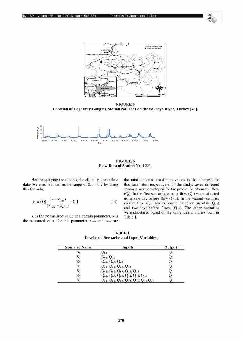
by PSP Volume 25 – No. 2/2016, pages 565-579 Fresenius Environmental Bulletin
570
FIGURE 5
Location of Dogancay Gauging Station No. 1221 on the Sakarya River, Turkey [45].
0
20
40
60
10.01.89 10.01.90 10.01.91 10.01.92 10.01.93 10.01.94 10.01.95 10.01.96 10.01.97 10.01.98 10.01.99 10.01.00
Riv
erf
low
(m
3/s
)
Date
FIGURE 6
Flow Data of Station No. 1221.
Before applying the models, the all daily streamflow
datas were normalized in the range of 0,1 - 0,9 by using
this formula;
1.0)(
)(8.0
minmax
min
xx
xxxi
(14)
xi is the normalized value of a certain parameter, x is
the measured value for this parameter, xmin and xmax are
the minimum and maximum values in the database for
this parameter, respectively. In the study, seven different
scenario were developed for the prediction of current flow
(Qt). In the first scenario, current flow (Qt) was estimated
using one-day-before flow (Qt-1). In the second scenario,
current flow (Qt) was estimated based on one-day (Qt-1)
and two-days-before flows (Qt-2). The other scenarios
were structured based on the same idea and are shown in
Table 1.
TABLE 1
Developed Scenarios and Input Variables.
Scenario Name Inputs Output
S1 Qt-1 Qt
S2 Qt-1, Qt-2 Qt
S3 Qt-1, Qt-2, Qt-3 Qt
S4 Qt-1, Qt-2, Qt-3, Qt-4 Qt
S5 Qt-1, Qt-2, Qt-3, Qt-4, Qt-5 Qt
S6 Qt-1, Qt-2, Qt-3, Qt-4, Qt-5, Qt-6 Qt
S7 Qt-1, Qt-2, Qt-3, Qt-4, Qt-5, Qt-6, Qt-7 Qt
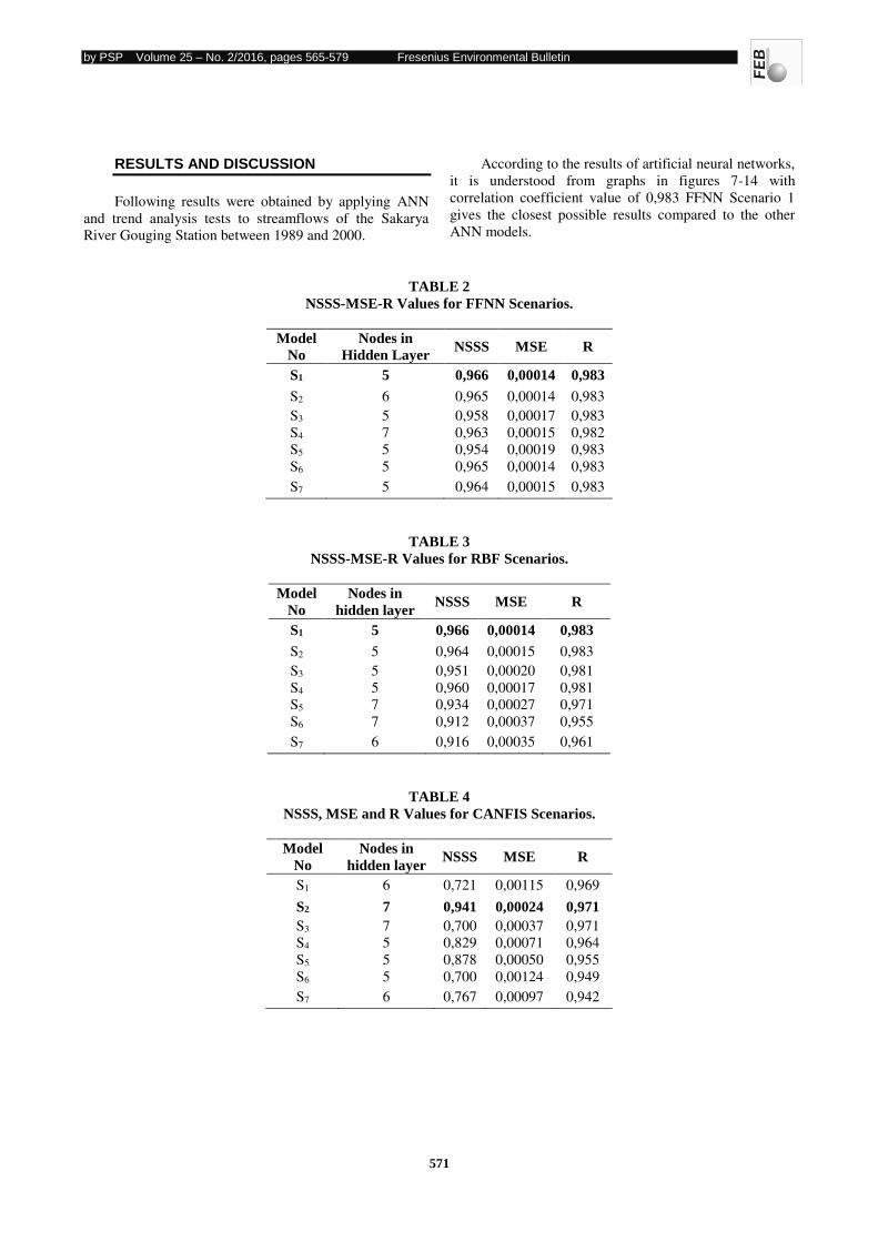
by PSP Volume 25 – No. 2/2016, pages 565-579 Fresenius Environmental Bulletin
571
RESULTS AND DISCUSSION
Following results were obtained by applying ANN
and trend analysis tests to streamflows of the Sakarya
River Gouging Station between 1989 and 2000.
According to the results of artificial neural networks,
it is understood from graphs in figures 7-14 with
correlation coefficient value of 0,983 FFNN Scenario 1
gives the closest possible results compared to the other
ANN models.
TABLE 2
NSSS-MSE-R Values for FFNN Scenarios.
Model
No
Nodes in
Hidden Layer NSSS MSE R
S1 5 0,966 0,00014 0,983
S2 6 0,965 0,00014 0,983
S3 5 0,958 0,00017 0,983
S4 7 0,963 0,00015 0,982
S5 5 0,954 0,00019 0,983
S6 5 0,965 0,00014 0,983
S7 5 0,964 0,00015 0,983
TABLE 3
NSSS-MSE-R Values for RBF Scenarios.
Model
No
Nodes in
hidden layer NSSS MSE R
S1 5 0,966 0,00014 0,983
S2 5 0,964 0,00015 0,983
S3 5 0,951 0,00020 0,981
S4 5 0,960 0,00017 0,981
S5 7 0,934 0,00027 0,971
S6 7 0,912 0,00037 0,955
S7 6 0,916 0,00035 0,961
TABLE 4
NSSS, MSE and R Values for CANFIS Scenarios.
Model
No
Nodes in
hidden layer NSSS MSE R
S1 6 0,721 0,00115 0,969
S2 7 0,941 0,00024 0,971
S3 7 0,700 0,00037 0,971
S4 5 0,829 0,00071 0,964
S5 5 0,878 0,00050 0,955
S6 5 0,700 0,00124 0,949
S7 6 0,767 0,00097 0,942
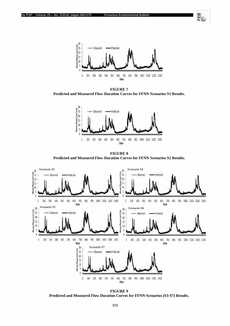
by PSP Volume 25 – No. 2/2016, pages 565-579 Fresenius Environmental Bulletin
572
FIGURE 7
Predicted and Measured Flow Duration Curves for FFNN Scenarios S1 Results.
FIGURE 8
Predicted and Measured Flow Duration Curves for FFNN Scenarios S2 Results.
FIGURE 9
Predicted and Measured Flow Duration Curves for FFNN Scenarios (S3-S7) Results.
Scenario S3
Scenario S5
Scenario S4
Scenario S6
Scenario S7
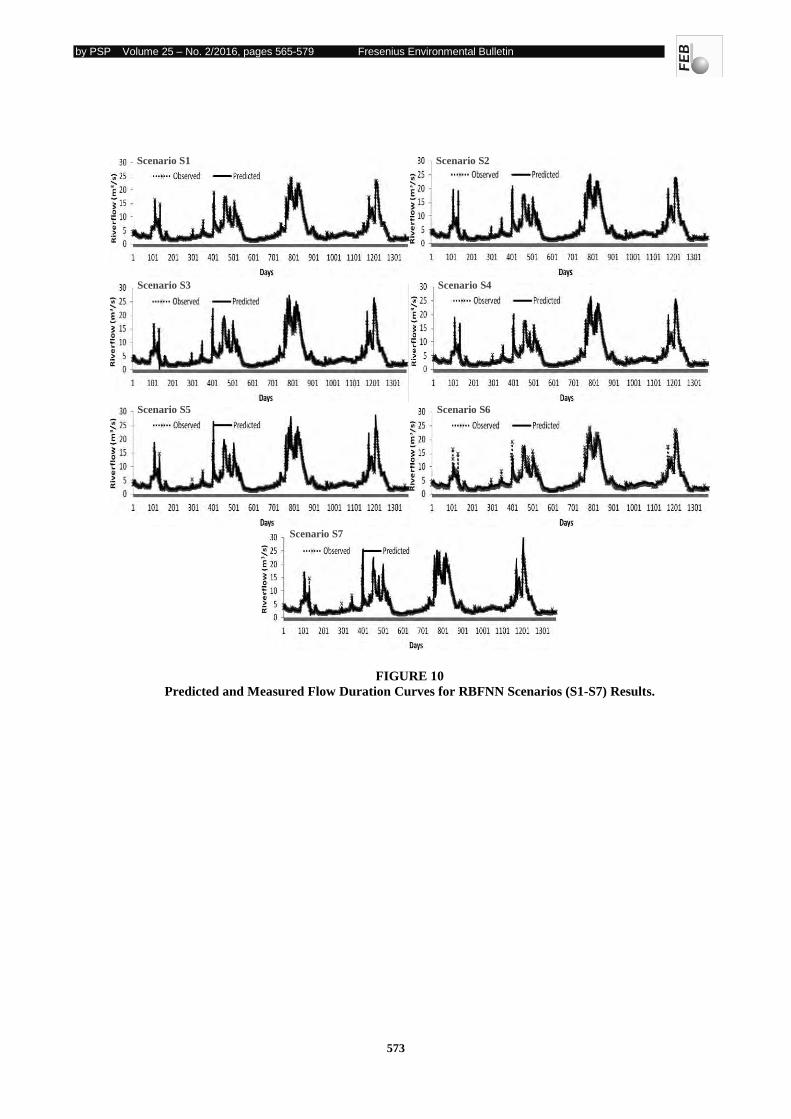
by PSP Volume 25 – No. 2/2016, pages 565-579 Fresenius Environmental Bulletin
573
FIGURE 10
Predicted and Measured Flow Duration Curves for RBFNN Scenarios (S1-S7) Results.
Scenario S6
Scenario S7
Scenario S5
Scenario S4 Scenario S3
Scenario S2 Scenario S1
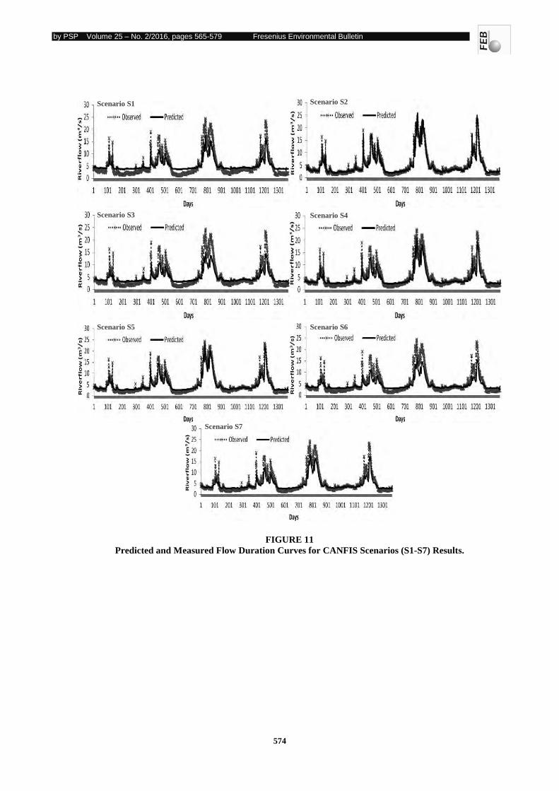
by PSP Volume 25 – No. 2/2016, pages 565-579 Fresenius Environmental Bulletin
574
FIGURE 11
Predicted and Measured Flow Duration Curves for CANFIS Scenarios (S1-S7) Results.
Scenario S1 Scenario S2
Scenario S3
Scenario S5 Scenario S6
Scenario S4
Scenario S7
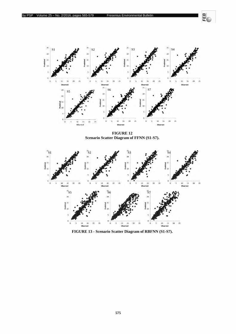
by PSP Volume 25 – No. 2/2016, pages 565-579 Fresenius Environmental Bulletin
575
FIGURE 12
Scenario Scatter Diagram of FFNN (S1-S7).
FIGURE 13 - Scenario Scatter Diagram of RBFNN (S1-S7).
S1 S2 S3 S4
S6 S7 S5
S1 S2 S3 S4
S5 S6 S7
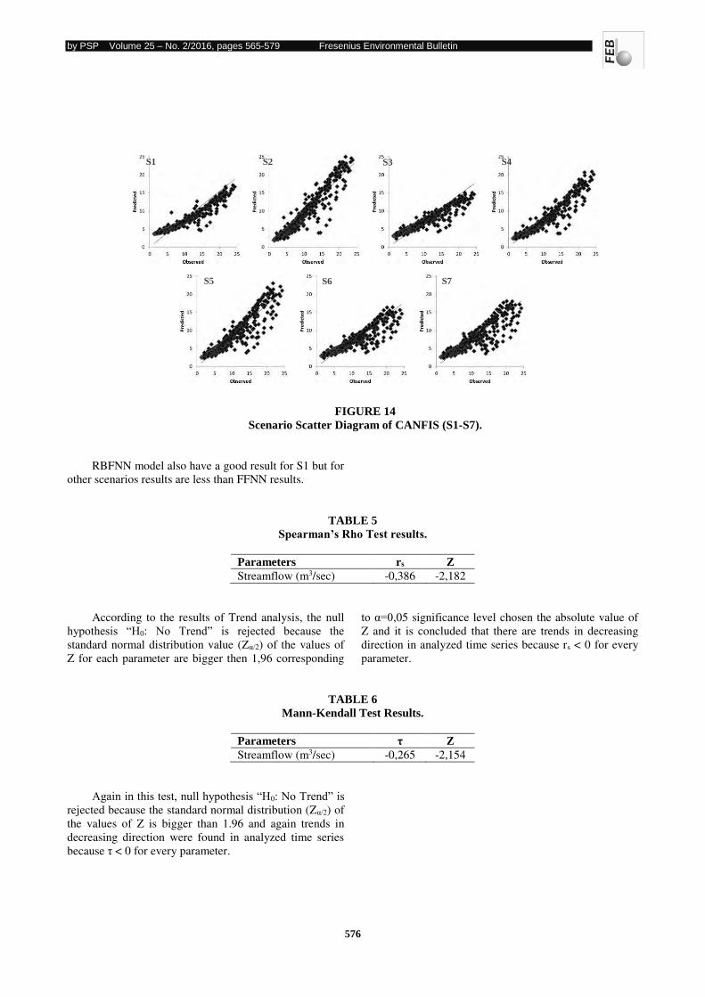
by PSP Volume 25 – No. 2/2016, pages 565-579 Fresenius Environmental Bulletin
576
FIGURE 14
Scenario Scatter Diagram of CANFIS (S1-S7).
RBFNN model also have a good result for S1 but for
other scenarios results are less than FFNN results.
TABLE 5
Spearman’s Rho Test results.
Parameters rs Z
Streamflow (m3/sec) -0,386 -2,182
According to the results of Trend analysis, the null
hypothesis “H0: No Trend” is rejected because the standard normal distribution value (Zα/2) of the values of
Z for each parameter are bigger then 1,96 corresponding
to α=0,05 significance level chosen the absolute value of
Z and it is concluded that there are trends in decreasing
direction in analyzed time series because rs < 0 for every
parameter.
TABLE 6
Mann-Kendall Test Results.
Parameters τ Z
Streamflow (m3/sec) -0,265 -2,154
Again in this test, null hypothesis “H0: No Trend” is
rejected because the standard normal distribution (Zα/2) of
the values of Z is bigger than 1.96 and again trends in
decreasing direction were found in analyzed time series
because τ < 0 for every parameter.
S1 S2 S3 S4
S5 S6 S7
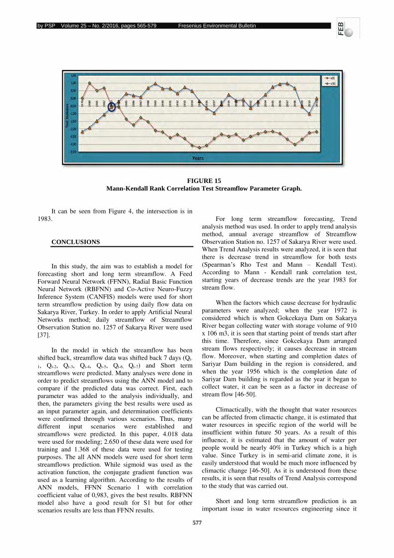
by PSP Volume 25 – No. 2/2016, pages 565-579 Fresenius Environmental Bulletin
577
FIGURE 15
Mann-Kendall Rank Correlation Test Streamflow Parameter Graph.
It can be seen from Figure 4, the intersection is in
1983.
CONCLUSIONS
In this study, the aim was to establish a model for
forecasting short and long term streamflow. A Feed
Forward Neural Network (FFNN), Radial Basic Function
Neural Network (RBFNN) and Co-Active Neuro-Fuzzy
Inference System (CANFIS) models were used for short
term streamflow prediction by using daily flow data on
Sakarya River, Turkey. In order to apply Artificial Neural
Networks method; daily streamflow of Streamflow
Observation Station no. 1257 of Sakarya River were used
[37].
In the model in which the streamflow has been
shifted back, streamflow data was shifted back 7 days (Qt-
1, Qt-2, Qt-3, Qt-4, Qt-5, Qt-6, Qt-7) and Short term
streamflows were predicted. Many analyses were done in
order to predict streamflows using the ANN model and to
compare if the predicted data was correct. First, each
parameter was added to the analysis individually, and
then, the parameters giving the best results were used as
an input parameter again, and determination coefficients
were confirmed through various scenarios. Thus, many
different input scenarios were established and
streamflows were predicted. In this paper, 4.018 data
were used for modeling; 2.650 of these data were used for
training and 1.368 of these data were used for testing
purposes. The all ANN models were used for short term
streamflows prediction. While sigmoid was used as the
activation function, the conjugate gradient function was
used as a learning algorithm. According to the results of
ANN models, FFNN Scenario 1 with correlation
coefficient value of 0,983, gives the best results. RBFNN
model also have a good result for S1 but for other
scenarios results are less than FFNN results.
For long term streamflow forecasting, Trend
analysis method was used. In order to apply trend analysis
method, annual average streamflow of Streamflow
Observation Station no. 1257 of Sakarya River were used.
When Trend Analysis results were analyzed, it is seen that
there is decrease trend in streamflow for both tests
(Spearman’s Rho Test and Mann – Kendall Test).
According to Mann - Kendall rank correlation test,
starting years of decrease trends are the year 1983 for
stream flow.
When the factors which cause decrease for hydraulic
parameters were analyzed; when the year 1972 is
considered which is when Gokcekaya Dam on Sakarya
River began collecting water with storage volume of 910
x 106 m3, it is seen that starting point of trends start after
this time. Therefore, since Gokcekaya Dam arranged
stream flows respectively; it causes decrease in stream
flow. Moreover, when starting and completion dates of
Sariyar Dam building in the region is considered, and
when the year 1956 which is the completion date of
Sariyar Dam building is regarded as the year it began to
collect water, it can be seen as a factor in decrease of
stream flow [46-50].
Climactically, with the thought that water resources
can be affected from climactic change, it is estimated that
water resources in specific region of the world will be
insufficient within future 50 years. As a result of this
influence, it is estimated that the amount of water per
people would be nearly 40% in Turkey which is a high
value. Since Turkey is in semi-arid climate zone, it is
easily understood that would be much more influenced by
climactic change [46-50]. As it is understood from these
results, it is seen that results of Trend Analysis correspond
to the study that was carried out.
Short and long term streamflow prediction is an
important issue in water resources engineering since it
by PSP Volume 25 – No. 2/2016, pages 565-579 Fresenius Environmental Bulletin
578
affects all of river engineering problems (e.g. flood
forecasting, sediment rating studies,), irrigation, reservoir
management policy and hydro-electric power stations
operating policy. Therefore, with the result of ANN
model, makes it possible to prediction of short term
streamflow. For long term streamflow prediction is
possible and give good result with Trend Analysis
method.
REFERENCES
[1] Trajkovic, S., Todorovic, B., Stankovic, M., (2003),
Forecast. Reference Evapotranspiration by Artificial
Neural Networks, ASCE J. Irrig. Drain, Eng., 129, 6,
454-457.
[2] Sudheer K.P., Gosain A.K., Rangan D.M., Saheb
S.M., (2002), Modelling Evaporation Using an
Artificial Neural Network Algorithm, Hydrological
Processes, 16, 3189-3202.
[3] Kisi, O., (2006), Generalized Regression Neural
Networks for Evapotranspiration Modeling. Hydro.
Sci. J., 51, 6, 1092-1105.
[4] Kisi, O., (2006), Evapotranspiration Estimation
Using Feed-Forward Neural Networks, Nordic
Hydro, 36, 1, 49-64.
[5] Dawson, W.C., Wilby. R., (1998), An Artificial
Neural Network Approach to Rainfall–Runoff
Modeling, Hydrological Sciences Journal, 43, 1, 47-
66.
[6] Solomatine, D.P., Dulal, K.N., (2003), Model Trees
as an Alternative to Neural Networks in Rainfall–Runoff Modeling. Hydrological Science Journal, 48,
3, 399-411.
[7] Raman, H., and Sunilkumar, N., (1995),
Multivariate Modelling of Water Resources Time
Series Using Artificial Neural Networks, Hydro. Sci.
J., 40, 2, 145-163.
[8] Zealand, C. M., Burn, D. H. and Simonovic, S. P.,
(1999), Short Term Stream Flow Forecasting Using
Artificial Neural Networks, Hydro., 214, 32-48.
[9] Sivakumar, B., Jayawardena, A.W. and Fernando,
T.M.K.G., (2002), River Flow Forecasting: Use of
Phase Space Reconstruction and Artificial Neural
Networks Approaches, Hydro. 265, 225-245.
[10] Cigizoglu, H. K., (2003), Estimation, Forecasting
and Extrapolation of River Flows by Artificial
Neural Networks. Hydro. Sci. J., 48, 3, 349-361.
[11] Saad, M., Bigras, P., Turgeon, A. and Duquette, R.,
(1996), Fuzzy Learning Decomposition for the
Scheduling of Hydroelectric Power Systems, Water
Res., 32, 1, 179-186.
[12] Jain, S.K., Das, D. and Srivastava, D.K., (1999).
Application of ANN for Reservoir Inflow Prediction
and Operation, Journal of Water Resources Planning
and Management, 125, 5, 263-271.
[13] Kisi, O., (2005), Suspended Sediment Estimation
Using Neuro-Fuzzy and Neural Network
Approaches, Hydro. Sci. J., 50, 4, 683-696.
[14] Cigizoglu, H.K. and Kisi, O., (2006), Methods to
Improve the Neural Network Performance in
Suspended Sediment Estimation, J. Hydro., 317,
221-238.
[15] Kisi O, (2009). Neural Network and Wavelet
Conjunction Model for Modelling Monthly Level
Fluctuations in Turkey, Hydro. Process, 23, 2081-
2092.
[16] Hagan, M.T. and Menhaj, M.B., (1994), Training
Feed Forward Networks with the Marquardt
Algorithm, IEEE Trans, Neural Networks, 6, 861-
867.
[17] Cybenco, G., (1989), Approximation by
Superposition of a Sigmoidal Function. Mathematics
of Control, Signals and Systems 2, 303-314.
[18] Hornik, K., Stinchcombe, M. and White, H. (1989),
Multilayer Feed Forward Networks are Universal
Approximators, Neural Networks 2, 359-366.
[19] Sonmez, O., Dogan, E., Ceribasi, G. and Demir, S.
(2013), Impact of Climate Change on the Daily
Water Level Fluctuation of Lake Sapanca, Journal of
Fresenius Environmental Bulletin, 22, 7, 1895-1903.
[20] Cybenco, G., (1989), Approximation by
Superposition of a Sigmoidal Function. Mathematics
of Control, Signals and Systems 2, 303-314.
[21] Hornik, K., Stinchcombe, M. and White, H. (1989),
Multilayer Feed Forward Networks are Universal
Approximators, Neural Networks 2, 359-366.
[22] Freiwan, M and Cigizoglu, H.K., (2005), Prediction
of Total Monthly Rainfall in Jordan Using Feed
Forward Backpropagation Method, Fresenius
Environmental Bulletin, 14, 142-151.
[23] Karakitsios, S.P., Hadjidakis, J., Kassomenos, P.A.
and Pilidis, G.A., (2006), Development of an
Artificial Neural Network to Predict Benzene
Concentrations in A Street Canyon, Fresenius
Environmental Bulletin, 15, 424-430.
[24] Diamantopoulou, M.J., Georgiou, P.E. and
Papamichail, D.M., (2007), Performance of Neural
Network Models with Kalman Learning Rule for
Flow Routing in A River System, Fresenius
Environmental Bulletin, 16, 1474-1484.
[25] Broomhead, D. and Lowe, D. (1988), Multivariable
functional interpolation and adaptive networks.
Complex Syst. 2, 321-355.
[26] Lee, G.C. and Chang, S.H. (2003), Radial basis
function networks applied to DNBR calculation in
digital core protection systems. Annals of Nuclear
Energy, 30, 1561-1572.
[27] Valez, O. And Langs. (2014), Feature Reduction
Using A RBF Network for Classification of
Learning Styles in First Year Engineering Students,
Ingeniare. Revista Chilena de Ingeniería, 22, 1, 140-
151.
by PSP Volume 25 – No. 2/2016, pages 565-579 Fresenius Environmental Bulletin
579
[28] Jang, J.S.R., Sun, C.T., Mizutani, E. (1997), Neuro-
Fuzzy and Soft Computing: A Comp. Approach to
Learning and Machine Intel. Prentice Hall,
Englewood Cliffs.
[29] Burrows, W.R., Walmsley, J., Montpetit, J., Faucher
M. (1998), Cart-Neuro-Fuzzy statistical data
modeling, Part 2: Results. In: Preprints, 14th
Conference on Probability and Statistics in the
Atmospheric Sci., Phoenix, AZ, 160-167. American
Met. Society, Boston, MA.
[30] Sengorur, B., Dede, C. and Dogan, E. (2014),
Separation of Stream Flow into Components
Through the Use of a Co-Active Neuro Fuzzy
Inference System (CANFIS), Fresenius
Environmental Bulletin, 23, 2279-2288.
[31] https://en.wikipedia.org/wiki (Access 26 June 2015).
[32] Buyukkaracigan, N. and Kahya, E. (1997), The
Dependency Analysis of Annual Peak Flows of
Streams in Konya Basin, In: Proc. of the
International Conference on Water Problems in the
Mediterranean Countries, Ankara, Turkey.
[33] Gumus, V. (2006), Evaluation of Firat River Basin
Streamflow by Trend Analysis, Institute of Science,
Department of Civil Engineering, Harran University,
Sanliurfa.
[34] Mann, H.B. (1945), Non-parametric Tests against
Trend.
[35] Kendall, M.G. (1975), Rank Correlation Methods,
London.
[36] Van Belle, G. and Hughes, J.P. (1984),
Nonparametric Tests for Trend in Water Quality, 1,
127–136.
[37] Partal, T., Kahya, E. and Karaca, M. (2003), Trend
Analysis of Lakes Region Precipitation Data, I.
National Hydrological Engineering Symposium,
Gumuldur, Izmir, Turkey.
[38] Gumus, V. and Yenigun, K. (2006), Evaluation of
Lower Fırat Basin Streamflow by Trend Analysis, 7th International Advances in Civil Engineering
Conference, Yildiz Technical University, Istanbul,
Turkey.
[39] Kalayci, S. and Kahya, E. (2006), Assessment of
streamflow variability modes in Turkey: 1964-1994,
Journal of Hydrology, 324, 163-177.
[40] Partal, T. and Kucuk, M. (2006), Long-Term trend
analysis using discrete wavelet components of
annual precipitations measurements in Marmara
Region (Turkey), Physics and Chemistry of the
Earth, 31, 1189-1200.
[41] Fiala, T. (2008), Statistical Characteristics and
Trends of Mean Annual and Monthly Discharges of
Czech Rivers in the Period 1961-2005. Journal of
Hydrology and Hydromechanics, 56, 133-140.
[42] Ceribasi, G. (2010), Estimation of Sediment
Discharge Transported in Sakarya River by Using
Trend Analysis Method. Institute of Science,
Department of Construction, Sakarya University,
Sakarya, Turkey.
[43] Ceribasi, G., Dogan, E. and Sonmez, O. (2013),
Evaluation of Sakarya River Streamflow and
Sediment Transport with Rainfall Using Trend
Analysis. Journal of Fresenius Environmental
Bulletin, 3A, 846-852.
[44] Ceribasi, G., Dogan, E. and Sonmez, O. (2014),
Evaluation of Meteorological and Hydrological Data
of Sapanca Basin by Trend Analysis Method.
Journal of Environmental Protection and Ecology, 2,
705-714.
[45] Isik, S., Dogan, E., Kalin, L., Sasal, M. and
Agiralioglu, N. (2008), Effects of Anthropogenic
Activities on the Lower Sakarya River, CATENA,
75, 2, 172-181.
[46] Atalay, A. and Ikiel, C. (2007), Trend analysis of
monthly and annual flow values of Sakarya River,
International symposium on Geography, 5-8 June,
Antalya, Turkey.
[47] Atalay, I. (1986), Applied Hydro geography - I, Ege
University, Faculty of Letters, Izmir.
[48] Bakir, H. (2003), Determination of Erzurum Ilica
Sinirbasi Creek Basin Precipitation and Streamflow
Characteristics, Ataturk University, Erzurum,
Turkey.
[49] Ikiel, C. and Kacmaz, M. (2007), Global Evolution;
Involving Change of Climate, Natural Resources and
Human Politics, 31st IMISE Conference, 2-7 July,
Naples, Italia.
[50] Yildiz, K., Sipahioglu, S. and Yilmaz, M. (2000)
Environmental Science, Gunduz Education and
Publishing, General Directorate of Electrical Power
Resources Survey and Development Administration,
Ankara, Turkey.
Received: 27.07.2015
Accepted: 06.12.2015
CORRESPONDING AUTHOR
Assist. Prof. Dr. Gokmen Ceribasi Sakarya University
Technology Faculty
Department of Civil Engineering
54187, Sakarya – TURKEY
e-mail: [email protected]
by PSP Volume 25 – No. 2/2016, pages 580-587 Fresenius Environmental Bulletin
580
EFFECT OF THE IRON CONCENTRATION ON THE
PROPERTIES OF AN ALUMINOSILICATE GLASS USED
FOR STORAGE OF RADIOACTIVE WASTE
D. Moudir1, S. Ikhaddalene2, N. Kamel1
, A. Benmounah3, F. Zibouche2, Y. Mouheb1
, F. Aouchiche1
1Nuclear Research Center of Algiers, Nuclear Technology Division, 2. Bd Frantz Fanon, BP 399, RP-Algiers, Algiers, Algeria 2Faculty of Science. Department of Chemistry, Railway Station Road - 35000 Boumerdes, Algeria
3Research Unit, Process Materials and Environment, University M'Hamed Bougurra, Boumerdes, 35000, Algeria
ABSTRACT
Aluminosilicate glasses doped with iron of the
valence state III have satisfactory properties, and
may be suitable as nuclear glasses, dedicated for
storage of radioactive waste solutions, cause of the
good reception capacities of actinides and / or
lanthanides, and excellent long-term performance
properties. In this work, a simplified
aluminosilicate glass composition: SiO2-Al2O3-
Fe2O3-MgO-Li2O-Na2O-K2O-Y2O3-ZrO2-La2O3-
MoO3 is synthesized by a batch method of double
melting of oxides at 1,450 ° C during 1h30min. The
influence of the content of Fe2O3 in the glass in the
interval: 0.50 to 7.00% was studied. Most of the
basic properties increase with the glass Fe2O3
content. The Archimedes density of the materials is
in the range 2.55-2.63 g / cm3, the molar volume in
the range 22.92 to 23.20 cm3/mol, Both X-ray
diffraction and scanning electron microscopy
analyses reveal a pure amorphous structure.
Infrared Spectroscopy Fourier Transform gave
spectra representative of the chemical composition
of the glasses studied. The values of Vickers
indentations are from 516 to 724 HV and Young
modulus around 0.330-1.840 GPa. The electrical
resistivity show a spring in the concentration of
3.0% Fe2O3, display both the combined effect of Fe
valence change and the mixed alkali effect (MAE)
in the glass. KEYWORDS: nuclear Glass, Fe, storage, radioactive waste, XRD, SEM.
INTRODUCTION
If one considers a typical nuclear fuel cycle,
majority of the radioactivity of the entire cycle is
concentrated in the so called high level waste
(HLW) [1]. Management of this waste is a major
challenge for nuclear scientists. They require
special treatment to ensure its isolation from human
environment for extended period of time. A variety
of matrix materials is available for the
immobilization of HLW. The choice of the
immobilization technology depends on the physical
and chemical nature of the waste and the
acceptance criteria for the long term storage and
disposal facility to which the waste will be
consigned. The main immobilization technologies
that are available commercially are cementation,
bituminization, and vitrification [2] . Vitrification is a particularly attractive
immobilization route because of the high chemical
durability (remain in a corrosive
environment). Furthermore, glasses have a flexible
microstructure which permits waste compositions.
Nuclear glasses must be durable against both self-
irradiation and water corrosion [3-5]. At an industrial scale, many glass systems are
employed in nuclear industries, mainly alkali
borosilicates and aluminoborosilicates glasses [6], each kind will exhibit a complex behavior
depending on its basic structure and the dopents
elements [7-9] With regard to their physico-chemical
properties, it has been demonstrated that these kinds
of glasses may be suitable candidates for minor
actinides and (REE elements or fission products)
[6]. Aluminosilicate glasses are widely used as
glasses with good mechanical, thermo-mechanical
and high chemical durability [10, 11], especially
when added with specific metals, like iron.
Many physical properties of oxide glasses
show non-linear behavior as a function of alkali
content, if one alkali type is gradually changed for
another alkali ion type [12-14], Which is referred
to the mixed alkali effect (MAE) [12].
In this paper we study the effect of iron
concentration ranging between 0.50 to 7.00 wt.%
on the properties of an aluminosilicate glass.
Lanthanum (La) and Yttrium (Y) was employed as
a lanthanide/actinide surrogate.
The materials are characterized by their
physical, microstructural, mechanical and electrical
properties. The glasses densities are measured for
calculating the molar volume, the amorphous
structure was confirmed by X-ray diffraction
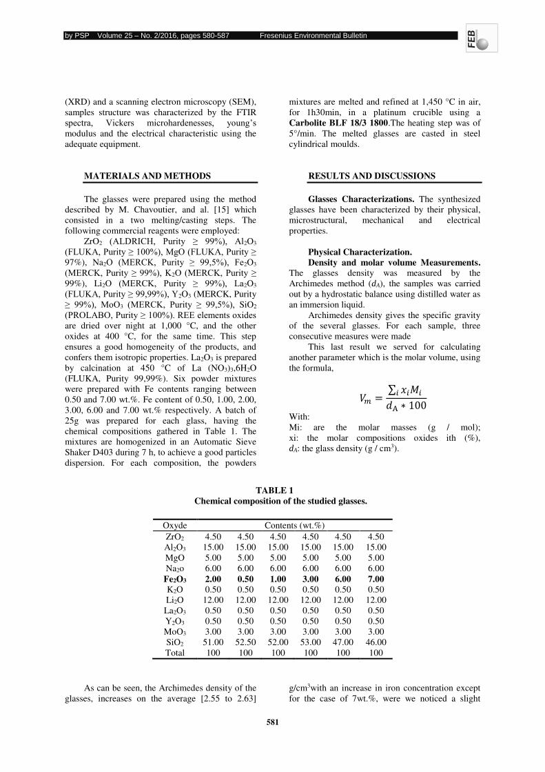
by PSP Volume 25 – No. 2/2016, pages 580-587 Fresenius Environmental Bulletin
581
(XRD) and a scanning electron microscopy (SEM),
samples structure was characterized by the FTIR
spectra, Vickers microhardenesses, young’s modulus and the electrical characteristic using the
adequate equipment.
MATERIALS AND METHODS
The glasses were prepared using the method
described by M. Chavoutier, and al. [15] which
consisted in a two melting/casting steps. The
following commercial reagents were employed:
ZrO2 (ALDRICH, Purity ≥ 99%), Al2O3
(FLUKA, Purity ≥ 100%), MgO (FLUKA, Purity ≥ 97%), Na2O (MERCK, Purity ≥ 99,5%), Fe2O3
(MERCK, Purity ≥ 99%), K2O (MERCK, Purity ≥ 99%), Li2O (MERCK, Purity ≥ 99%), La2O3
(FLUKA, Purity ≥ 99,99%), Y2O3 (MERCK, Purity
≥ 99%), MoO3 (MERCK, Purity ≥ 99,5%), SiO2
(PROLABO, Purity ≥ 100%). REE elements oxides are dried over night at 1,000 °C, and the other
oxides at 400 °C, for the same time. This step
ensures a good homogeneity of the products, and
confers them isotropic properties. La2O3 is prepared
by calcination at 450 °C of La (NO3)3,6H2O
(FLUKA, Purity 99,99%). Six powder mixtures
were prepared with Fe contents ranging between
0.50 and 7.00 wt.%. Fe content of 0.50, 1.00, 2.00,
3.00, 6.00 and 7.00 wt.% respectively. A batch of
25g was prepared for each glass, having the
chemical compositions gathered in Table 1. The
mixtures are homogenized in an Automatic Sieve
Shaker D403 during 7 h, to achieve a good particles
dispersion. For each composition, the powders
mixtures are melted and refined at 1,450 °C in air,
for 1h30min, in a platinum crucible using a
Carbolite BLF 18/3 1800.The heating step was of
5°/min. The melted glasses are casted in steel
cylindrical moulds.
RESULTS AND DISCUSSIONS
Glasses Characterizations. The synthesized
glasses have been characterized by their physical,
microstructural, mechanical and electrical
properties.
Physical Characterization. Density and molar volume Measurements.
The glasses density was measured by the
Archimedes method (dA), the samples was carried
out by a hydrostatic balance using distilled water as
an immersion liquid.
Archimedes density gives the specific gravity
of the several glasses. For each sample, three
consecutive measures were made
This last result we served for calculating
another parameter which is the molar volume, using
the formula,
�� = ∑ ����� �A ∗
With:
Mi: are the molar masses (g / mol);
xi: the molar compositions oxides ith (%),
dA: the glass density (g / cm3).
TABLE 1 Chemical composition of the studied glasses.
Oxyde Contents (wt.%)
ZrO2 4.50 4.50 4.50 4.50 4.50 4.50
Al2O3 15.00 15.00 15.00 15.00 15.00 15.00
MgO 5.00 5.00 5.00 5.00 5.00 5.00
Na2o 6.00 6.00 6.00 6.00 6.00 6.00
Fe2O3 2.00 0.50 1.00 3.00 6.00 7.00 K2O 0.50 0.50 0.50 0.50 0.50 0.50
Li2O 12.00 12.00 12.00 12.00 12.00 12.00
La2O3 0.50 0.50 0.50 0.50 0.50 0.50
Y2O3 0.50 0.50 0.50 0.50 0.50 0.50
MoO3 3.00 3.00 3.00 3.00 3.00 3.00
SiO2 51.00 52.50 52.00 53.00 47.00 46.00
Total 100 100 100 100 100 100
As can be seen, the Archimedes density of the
glasses, increases on the average [2.55 to 2.63]
g/cm3with an increase in iron concentration except
for the case of 7wt.%, were we noticed a slight
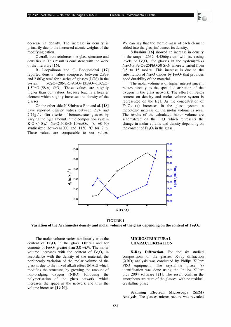
by PSP Volume 25 – No. 2/2016, pages 580-587 Fresenius Environmental Bulletin
582
decrease in density. The increase in density is
primarily due to the increased atomic weights of the
modifying cation.
Overall, iron reinforces the glass structure and
densifies it .This result is consistent with the work
of the literature [16].
R. Laopaiboon and C. Bootjomchai [17]
reported density values comprised between 2.839
and 2.863g /cm3 for a series of glasses (LGS) in the
system xCeO2-20Na2O-Al2O3-13B2O3-6.5CaO-
1.5PbO-(58-x) SiO2. These values are slightly
higher than our values, because lead is a heavier
element which slightly increases the density of the
glasses.
On the other side N.Srinivasa Rao and al. [18] have reported density values between 2.24 and
2.74g / cm3for a series of boroarsenates glasses, by
varying the K2O amount in the composition system
K2O-x(40-x) Na2O-50B2O3-10As2O3, (x =0-40)
synthesized between1000 and 1150 °C for 2 h.
These values are comparable to our values.
We can say that the atomic mass of each element
added into the glass influences its density.
S.Ibrahim [16] showed an increase in density
in the range 4.2632 -4.4566g / cm3 with increasing
levels of Fe2O3, for glasses in the system(25-x)
Na2O-x Fe2O3-25PbO-50 SiO2 where x varied from
0.5 to 15 mol.%. This increase is due to the
substitution of Na2O oxides by Fe2O3 that provides
good durability of the material.
The molar volume is of higher interest since it
relates directly to the special distribution of the
oxygen in the glass network. The effect of Fe2O3
content on density and molar volume system is
represented on the fig1. As the concentration of
Fe2O3 (x) increases in the glass system, a
monotonic increase of the molar volume is seen.
The results of the calculated molar volume are
schematized on the Fig1 which represents the
change in molar volume and density depending on
the content of Fe2O3 in the glass.
0 2 4 6 8
2,54
2,56
2,58
2,60
2,62
2,64
%(Fe2O
3)
d A (g
/ cm
3 )
22,80
22,85
22,90
22,95
23,00
23,05
23,10
23,15
23,20
23,25
Vm
(cm3 / m
ol )
FIGURE 1 Variation of the Archimedes density and molar volume of the glass depending on the content of Fe2O3.
The molar volume varies nonlinearly with the
content of Fe2O3 in the glass. Overall and for
contents of Fe2O3 greater than 3.0 wt.%, The molar
volume increases with the content of Fe2O3 in
accordance with the density of the material. the
nonlinearly variation of the molar volume of the
glass is due to the mixed alkali effect (MAE) which
modifies the structure, by growing the amount of
non-bridging oxygen (NBO) following the
polymerisation of the glass network, which
increases the space in the network and thus the
volume increases [19,20].
MICROSTRUCTURAL CHARACTERIZATION X-Ray Diffraction. For the six studied
compositions of the glasses, X-ray diffraction
(XRD) analysis was conducted by Philips X’Pert PRO equipment. The crystalline phase (s)
identification was done using the Philips X’Pert plus 2004 software [21]. The result confirm the
amorphous structure of the glasses, with no residual
crystalline phase. Scanning Electron Microscopy (SEM)
Analysis. The glasses microstructure was revealed
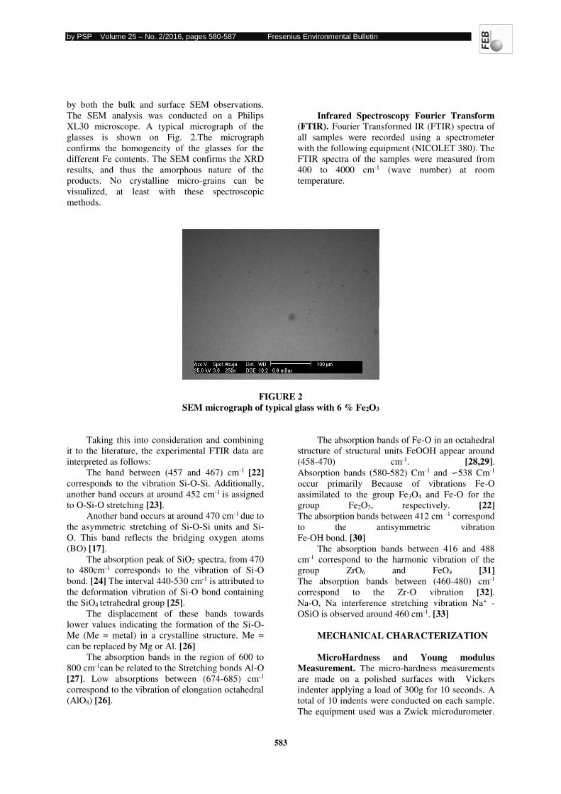
by PSP Volume 25 – No. 2/2016, pages 580-587 Fresenius Environmental Bulletin
583
by both the bulk and surface SEM observations.
The SEM analysis was conducted on a Philips
XL30 microscope. A typical micrograph of the
glasses is shown on Fig. 2.The micrograph
confirms the homogeneity of the glasses for the
different Fe contents. The SEM confirms the XRD
results, and thus the amorphous nature of the
products. No crystalline micro-grains can be
visualized, at least with these spectroscopic
methods.
Infrared Spectroscopy Fourier Transform
(FTIR). Fourier Transformed IR (FTIR) spectra of
all samples were recorded using a spectrometer
with the following equipment (NICOLET 380). The
FTIR spectra of the samples were measured from
400 to 4000 cm-1 (wave number) at room
temperature.
FIGURE 2 SEM micrograph of typical glass with 6 % Fe2O3
Taking this into consideration and combining
it to the literature, the experimental FTIR data are
interpreted as follows:
The band between (457 and 467) cm-1 [22] corresponds to the vibration Si-O-Si. Additionally,
another band occurs at around 452 cm-1 is assigned
to O-Si-O stretching [23]. Another band occurs at around 470 cm-1 due to
the asymmetric stretching of Si-O-Si units and Si-
O. This band reflects the bridging oxygen atoms
(BO) [17]. The absorption peak of SiO2 spectra, from 470
to 480cm-1 corresponds to the vibration of Si-O
bond. [24] The interval 440-530 cm-1 is attributed to
the deformation vibration of Si-O bond containing
the SiO4 tetrahedral group [25]. The displacement of these bands towards
lower values indicating the formation of the Si-O-
Me (Me = metal) in a crystalline structure. Me =
can be replaced by Mg or Al. [26] The absorption bands in the region of 600 to
800 cm-1can be related to the Stretching bonds Al-O
[27]. Low absorptions between (674-685) cm-1
correspond to the vibration of elongation octahedral
(AlO8) [26].
The absorption bands of Fe-O in an octahedral
structure of structural units FeOOH appear around
(458-470) cm-1. [28,29]. Absorption bands (580-582) Cm-1 and ∽538 Cm-1
occur primarily Because of vibrations Fe-O
assimilated to the group Fe3O4 and Fe-O for the
group Fe2O3, respectively. [22] The absorption bands between 412 cm -1 correspond
to the antisymmetric vibration
Fe-OH bond. [30] The absorption bands between 416 and 488
cm-1 correspond to the harmonic vibration of the
group ZrO6 and FeO4 [31] The absorption bands between (460-480) cm-1
correspond to the Zr-O vibration [32]. Na-O, Na interference stretching vibration Na+ -
OSiO is observed around 460 cm-1. [33]
MECHANICAL CHARACTERIZATION MicroHardness and Young modulus
Measurement. The micro-hardness measurements
are made on a polished surfaces with Vickers
indenter applying a load of 300g for 10 seconds. A
total of 10 indents were conducted on each sample.
The equipment used was a Zwick microdurometer.
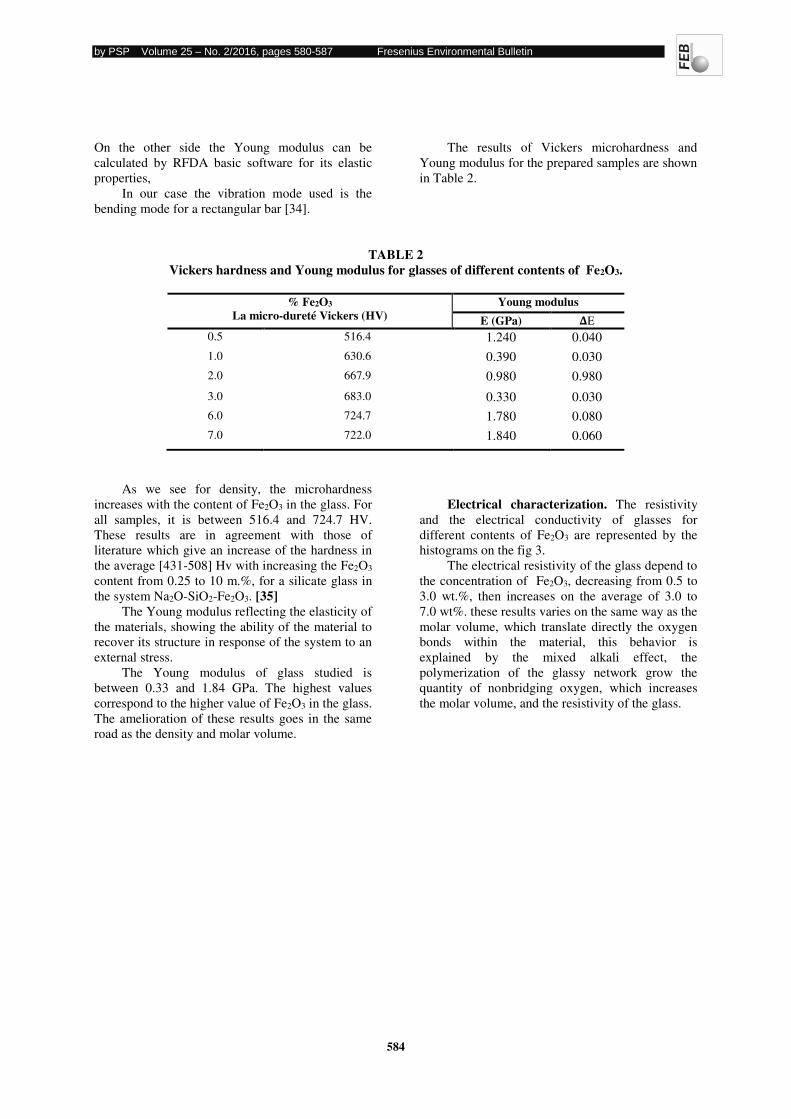
by PSP Volume 25 – No. 2/2016, pages 580-587 Fresenius Environmental Bulletin
584
On the other side the Young modulus can be
calculated by RFDA basic software for its elastic
properties,
In our case the vibration mode used is the
bending mode for a rectangular bar [34].
The results of Vickers microhardness and
Young modulus for the prepared samples are shown
in Table 2.
TABLE 2 Vickers hardness and Young modulus for glasses of different contents of Fe2O3.
% Fe2O3
La micro-dureté Vickers (HV) Young modulus
E (GPa) �E
0.5 516.4 1.240 0.040
1.0 630.6 0.390 0.030
2.0 667.9 0.980 0.980
3.0 683.0 0.330 0.030
6.0 724.7 1.780 0.080
7.0 722.0 1.840 0.060
As we see for density, the microhardness
increases with the content of Fe2O3 in the glass. For
all samples, it is between 516.4 and 724.7 HV.
These results are in agreement with those of
literature which give an increase of the hardness in
the average [431-508] Hv with increasing the Fe2O3
content from 0.25 to 10 m.%, for a silicate glass in
the system Na2O-SiO2-Fe2O3. [35] The Young modulus reflecting the elasticity of
the materials, showing the ability of the material to
recover its structure in response of the system to an
external stress.
The Young modulus of glass studied is
between 0.33 and 1.84 GPa. The highest values
correspond to the higher value of Fe2O3 in the glass.
The amelioration of these results goes in the same
road as the density and molar volume.
Electrical characterization. The resistivity
and the electrical conductivity of glasses for
different contents of Fe2O3 are represented by the
histograms on the fig 3. The electrical resistivity of the glass depend to
the concentration of Fe2O3, decreasing from 0.5 to
3.0 wt.%, then increases on the average of 3.0 to
7.0 wt%. these results varies on the same way as the
molar volume, which translate directly the oxygen
bonds within the material, this behavior is
explained by the mixed alkali effect, the
polymerization of the glassy network grow the
quantity of nonbridging oxygen, which increases
the molar volume, and the resistivity of the glass.
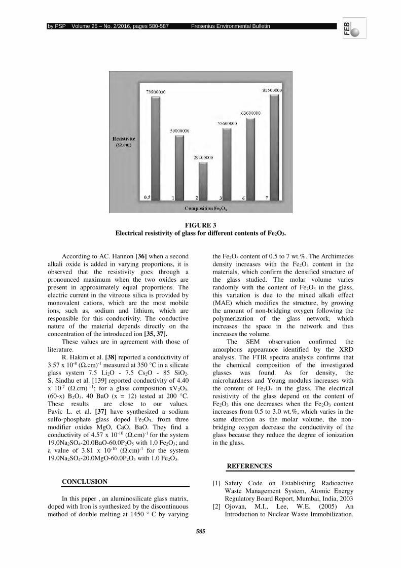
by PSP Volume 25 – No. 2/2016, pages 580-587 Fresenius Environmental Bulletin
585
FIGURE 3 Electrical resistivity of glass for different contents of Fe2O3.
According to AC. Hannon [36] when a second
alkali oxide is added in varying proportions, it is
observed that the resistivity goes through a
pronounced maximum when the two oxides are
present in approximately equal proportions. The
electric current in the vitreous silica is provided by
monovalent cations, which are the most mobile
ions, such as, sodium and lithium, which are
responsible for this conductivity. The conductive
nature of the material depends directly on the
concentration of the introduced ion [35, 37]. These values are in agreement with those of
literature.
R. Hakim et al. [38] reported a conductivity of
3.57 x 10⁻⁸ (Ω.cm)-1 measured at 350 °C in a silicate
glass system 7.5 Li2O - 7.5 Cs2O - 85 SiO2.
S. Sindhu et al. [139] reported conductivity of 4.40
x 10-7 (Ω.cm) -1; for a glass composition xV2O5.
(60-x) B2O3. 40 BaO (x = 12) tested at 200 °C.
These results are close to our values.
Pavic L. et al. [37] have synthesized a sodium
sulfo-phosphate glass doped Fe2O3, from three
modifier oxides MgO, CaO, BaO. They find a
conductivity of 4.57 x 10⁻¹⁰ (Ω.cm)-1 for the system
19.0Na2SO4-20.0BaO-60.0P2O5 with 1.0 Fe2O3; and
a value of 3.81 x 10⁻¹⁰ (Ω.cm)-1 for the system
19.0Na2SO4-20.0MgO-60.0P2O5 with 1.0 Fe2O3.
CONCLUSION
In this paper , an aluminosilicate glass matrix,
doped with Iron is synthesized by the discontinuous
method of double melting at 1450 ° C by varying
the Fe2O3 content of 0.5 to 7 wt.%. The Archimedes
density increases with the Fe2O3 content in the
materials, which confirm the densified structure of
the glass studied. The molar volume varies
randomly with the content of Fe2O3 in the glass,
this variation is due to the mixed alkali effect
(MAE) which modifies the structure, by growing
the amount of non-bridging oxygen following the
polymerization of the glass network, which
increases the space in the network and thus
increases the volume.
The SEM observation confirmed the
amorphous appearance identified by the XRD
analysis. The FTIR spectra analysis confirms that
the chemical composition of the investigated
glasses was found. As for density, the
microhardness and Young modulus increases with
the content of Fe2O3 in the glass. The electrical
resistivity of the glass depend on the content of
Fe2O3 this one decreases when the Fe2O3 content
increases from 0.5 to 3.0 wt.%, which varies in the
same direction as the molar volume, the non-
bridging oxygen decrease the conductivity of the
glass because they reduce the degree of ionization
in the glass.
REFERENCES
[1] Safety Code on Establishing Radioactive
Waste Management System, Atomic Energy
Regulatory Board Report, Mumbai, India, 2003
[2] Ojovan, M.I., Lee, W.E. (2005) An
Introduction to Nuclear Waste Immobilization.
by PSP Volume 25 – No. 2/2016, pages 580-587 Fresenius Environmental Bulletin
586
Elsevier Science Publishers B.V, Amsterdam,
The Netherlands, p.315.
[3] B. Grambow, Nuclear waste glasses: How
durable? Elements, vol. 2, n°(6) p.357-364,
(2006)
[4] Combarieu, G. D. (2007) Altération du verre de
confinement de déchets type R7T7 en
condition de stockage géologique, University
of Paris XI
[5] Zaoui, A. (2000) Academy of sciences.
materials for the nuclear, RST report No. 5,
Tec. and Doc. (eds.) Lavoisier, Paris.
[6] Chouard, N., Caurant, D., Majérus, O.,
Dussossoy, J.L., Ledieu, A., Peuget, S. (2011)
Effect of neodymium oxide onthe solubility of
MoO3 in an aluminoborosilicate glass. Journal
of Non-Crystalline Solids, 357 (14) 2752-2762.
[7] Quintas, A., Caurant, D., Majérus, O.,
Dussossoy, J.L., Charpentier ,T. (2008) Effect
of changing the rare earth cation typeon the
structure and crystallisationbehaviour of
analuminoborosilicate glass. European Journal
of Glass Science Technology B, 49 (4) 192-
197.
[8] Quintas, A., Majérus, O., Caurant, D.,
Dussossoy, J.L., Vermaut, P. (2007)
Crystallization of a rare earth-rich
aluminoborosilicate glass with varying
CaO/Na2O ratio. Journal of the American
Ceramic Society, 90 (3) 712-719.
[9] Quintas, A., Charpentier, T., Majérus, O.,
Caurant, D., Dussossoy, J.L., Vermaut, P.,
(2007) NMR study of a rare-earth
aluminoborosilicate glass with varying CaO-to-
Na2O ratio. Applied Magnetic Resonance, 32
(4) 613-634.
[10] Leturcq, G., Berger, G., Advocat, T., Fillet, C.,
Halgand C., Vernaz, E. (1997) Chemical
durability of aluminosilicate glasses containing
low solubility chemical elements, C-MRS Int.
Symp. Proc., DOI : 10.1557/proc-p: 506-199.
[11] Scholze, H. (1959) Der Einbau des Wassers in
Glӓsern. Glastech. Ber, 32 (4) 142-152.
[12] Isard, J.O. (1969) The mixed alkali effect in
glass. Journal of Non-Crystalline Solids, 1 (3)
235-261.
[13] Day, D.E. (1976) Mixed alkali glasses - their
properties and uses. Journal of Non-Crystalline
Solids, 21 (3) 343-372. [14] Ingram, M.D. (1987) Ionic Conductivity in
Glass. Physics and Chemistry of Glasses, 28
(6) 215-234.
[15] Chavoutier, M., Caurant, D., Majérus, O.,
Boulesteix, R., Loiseau, P., Jousseaume, C.,
Brunet , E., Lecomte , E. (2014) Effect of TiO2
content on the crystallization and the color of
(ZrO2,TiO2)-doped Li2O–Al2O3–SiO2 glasses.
Journal of Non Crystalline Solids, 384, 15–24.
[16] Ibrahim, S., Morsi, M.M. (2013) Effect of
increasing Fe2O3 content on the chemical
durability and infrared spectra of (25 - x)
Na2O-x Fe2O3-25PbO-50SiO2 glasses.
Materials Chemistry and Physics, 138 (2-3)
417-966.
[17] Laopaiboon, R., Bootjomchai, C. (2014)
Radiation effects on structural properties of
glass by using ultrasonic techniques and FTIR
spectroscopy: A comparison between local
sand and SiO2. Annals of Nuclear Energy, 68,
220-227.
[18] Rao, N.S., Bale, S., Purnima, M., Kumar, K.
S., Rahman, S. (2007) Mixed alkali effect in
boroarsenate glasses. Journal of Physical and
Chemistry of Solids, 68 (7) 1354-1358.
[19] Duffy, J.A., Ingram, M.D. (1975) Optical
basicity-IV: Influence of electronegativity on
the Lewis basicity and solvent properties of
molten oxyanion salts and glasses. Journal of
Inorganic and Nuclear Chemistry, 37 (5) 1203-
1206.
[20] Padmaja, G., Kistaiah, P. (2009) Infrared and
Raman spectroscopic studies on Alkali Borate
Glasses: Evidence of Mixed Alkali Effect.
Journal of Physical and Chemistry, 113 (11)
2397-2004.
[21] JCPDS data Philips X’Pert High Score Package, Diffraction data CD-ROM. (2004)
International Center for Diffraction Data,
Newtown Square PA.
[22] Palanivel, R., Velraj, G. (2007) FTIR and FT-
Raman spectroscopic studies of fired clay
artifacts recently excavated in Tamilnadu India.
Indian Journal of Pure & Applied Physics, 45
(6) 501-508.
[23] Zibouche, F., Boudissa, N., irekti, A., Abadlia,
M.T. (2013) Géopolymérisation
d’aluminosilicates. Influences des rapports
Silice/Alumine. Journal of Materials, Processes
and environment, 01,147-156.
[24] Atalay, S., Adiguzel, H.I., Atalay, F. (2001)
Infrared absorption study of Fe2O3–CaO–SiO2
glass ceramics. Materials Science and
Engineering A, 304–306, p796–799.
[25] El-Egili, K. (2003) Infrared studies of Na2O-
B2O3-SiO2 and Al2O3-Na2O-B2O3-
SiO2 glasses. Physica B : Condensed Matter,
325, 340–348,
[26] Petrovic, R., Janackovic, D., Zec, S., Drmanic,
S., Kostic-Gvozdenovic, L.J. (2003)
Crystallization behavior of alkoxy-derivrd
cordierite gels Crystallization Behavior of
Alkoxy-Derived Cordierite Gels. Journal of
by PSP Volume 25 – No. 2/2016, pages 580-587 Fresenius Environmental Bulletin
587
Sol-Gel Science and Technology, 28 (1) 111-
118.
[27] Lin, S.L., Hwang, C.S. (1996) Structures of
CeO2Al2O3SiO2 glasses. Journal of Non-
Crystalline Solids, 202, (1-2) 61-67.
[28] Cakić, M. D., Nikolić, G. S., Ilić, Lj. A. (2002)FTIR spectra of iron(III) complexes
with dextran pullulan and inulin oligomers.
Bulletin of the Chemists and Technologists of
Macedonia, 21 (2) 135-146. [29] Singh, S. P., Chakradhar, R.P.S., Rao, J.L.,
Karmakar, B. (2010) EPR, FTIR, Optical
absorption and photoluminescence studies of
Fe2O3 and CeO2 doped ZnO-Bi2O3-B2O3
glasses. Journal of Alloys and Compounds, 493
(1) 256–262.
[30] Cambier, P. (1986) Infrared Study of Goethites
of Varying crytallinity and Particle, siza : I.
Interpretation of OH and Lattice vibration
frequencies. Clay Minerals, 21 (2) 191-200.
[31] Pascuta, P., Borodi, G., Jumate, N., Vida-
Simiti, I., Viorel, D., Culea, E. (2010) The
structural role of manganese ions in some zinc
phosphate glasses and glass ceramics. Journal
of Alloys and Compounds, 504 (2) 479-483.
[32] Joe, H., Vasudevan, A., Aruldhas, G.,
Damodaran, A., Warrier, K. (1997) FTIR as a
tool to study high-temperature phase formation
in sol-gel aluminium titanate. Journal of Solid
State Chemistry, 131 (1) 181-184.
[33] King, P.L., Ramsey, M.S., Swayze, G.A.
(2004) Infrared Spectroscopy in Geochemistry
Exploration Geochemistry and Remote
Sensing. The 49th annual meeting of the
Mineralogical Association of Canada, 33, p 93-
133. Proceedings.
[34] IMCE. Integrated material control engineering
n.v. MANUAL Version 1.1 RFDA basic, PDF
[35] Bansal, N.P. Doremus, R. H. (1986) Handbook
of Glass Properties. Materials Engineering
Department Rensselaer Polytechnic Institute,
United Kingdom Edition published by
Academic Press INC. (LONDON) LTD. 24-28
Oval Road.
[36] Hannon, A.C., Parker, J.M. (2002) The use of
bond-valence parameters in interpreting glass
diffraction results. Physics and Chemistry of
Glasses, 43C (6) 6-12.
[37] Pavic, L., Moguš-Milankovic, A., Raghava
Rao, P., Šantic, A., Ravi Kumar, V., Veeraiah, N. (2014) Effect of alkali-earth modifier ion on
electrical, dielectric and spectroscopic
properties of Fe2O3 doped Na2SO4AMOAP2O5
glass system. Journal of Alloys and
Compounds, 604, 352–362.
[38] Hakim, R. M., Uhlmann, D. R. (1973) Physics
and Chemistry of Glasses, 14, 81.
Received: 27.07.2015 Accepted: 08.01.2016 CORRESPONDING AUTHOR
D. Moudir Nuclear Research Center of Algiers
Nuclear Technology Division
2. Bd Frantz Fanon, BP 399
RP-Algiers, Algiers – ALGERIA
by PSP Volume 25 – No. 2/ 2016, pages 588-601 Fresenius Environmental Bulletin
588
ADSORPTION OF Cr(VI) ONTO BIOCHARS DERIVED FROM TYPICAL VEGETABLE OIL CROP BIOMASSES
ORIGINATING IN LOESS AREAS
Baowei Zhao, Xiaying Shi, Fengfeng Ma
School of Environmental and Municipal Engineering, Lanzhou Jiaotong University, Lanzhou 730070, P. R. China
ABSTRACT
In this study, four types of biomasses
originating in loess areas (flax straw, rape straw,
flaxseed tailing and rapeseed tailing) were collected
and converted into biochars through pyrolysis. The
biomasses pyrolyzed from flax straw at 600 °C
(FS600), rape straw at 600 °C (RS600), flaxseed
tailing at 400 °C (FT400) and rapeseed tailing at
400 °C (RT400) were selected and characterized.
The adsorptive performance of Cr(VI) onto the four
types of biochars was investigated using the batch
equilibrium method. The effects of solution pH,
temperature, contact time, and initial Cr(VI)
concentration on Cr(VI) adsorption were tested.
The results showed that Cr(VI) adsorption by the
biochars was highly pH-dependent, and the Cr(VI)
adsorption capacity decreased with increasing pH
values. The adsorption kinetics followed the
pseudo-second-order equation. The adsorption data
were well described by the Langmuir isotherm. The
maximum adsorptive capacities of Cr(VI) were
26.7, 30.8, 33.0 and 29.2 mg/g by FS600, RS600,
FT400 and RT400, respectively. The adsorptive
capacity increased with increasing temperature,
indicating that the adsorption processes were
mostly endothermic chemical processes. According
to FTIR, the differences in the surface structures
and functional groups from before and after Cr(VI)
adsorption showed that the mechanisms of Cr(VI)
adsorption onto the biochars primarily included
chemical bonding and electrostatic attraction.
KEYWORDS:
biomass; biochar; characterization; Cr(VI); adsorption
INTRODUCTION
Loess is widespread, accounting for one-tenth
of the global land area. Approximately 640
thousand km2 of loess area is spread over China’s topography, especially in northwestern China. The
loose structure, large porosity and water
permeability, low agglomerating force and organic
matter content result in nutrient leaching from the
loess soils, causing it to have poor quality [1].
Moreover, there are excessive concentrations of
heavy metals in farmland soils in loess areas,
resulting primarily from irrigation using industrial
wastewater, the disposal of solid waste (e.g.,
sludge, garbage, etc.), the use of agrochemicals and
fertilizers, and atmospheric deposition [2, 3].
Improvement and remediation of loess soils are of
utmost importance and urgency.
Biochar (BC) is a carbon-rich solid by-product
of the pyrolysis of biomass under oxygen-free and
low temperature conditions. When applied to soils,
biochar’s proven ability to remain stable against chemical and biological degradation renders it an
innovative method of mitigating climate change [4,
5]. In addition, biochar can improve soil
productivity because it can be a valuable nitrogen
and phosphorous source, and it affects soil cation
exchange capacity, pH, and the retention of water
and nutrients [6, 7]. The porous structure,
negatively charged surface and large number of
functional groups on the surface of biochar causes it
to be a remarkable adsorbent and immobilizing
agent for contaminants when it is added to soils,
providing a promising in-situ alternative to
remediate soils contaminated with heavy metals [8,
9]. Therefore, biochars should be applied to loess
soil to improve the soil structure and properties,
increase the soil’s water holding capacity, improve soil fertility and enhance crop yield. Meanwhile, it
is also expected that the use of biochars as an
amendment will control the migration,
transformation and bioavailability behaviors of
heavy metal pollutants and will ensure the safety of
agricultural products.
Generally, chromium is found in nature in the
trivalent and hexavalent forms. Of its two oxidation
states, the hexavalent form is of particular concern
because it is 100 times more toxic than the trivalent
form and exerts adverse effects on humans [10].
For this reason, much attention has been paid to
removal of Cr(VI) from waste water [11-15].
However, in recent years, with the development of
modern industries, including electroplating,
tanning, textile, painting and metal finishing, large
quantities of chromium compounds have entered
by PSP Volume 25 – No. 2/ 2016, pages 588-601 Fresenius Environmental Bulletin
589
into loess soils through untreated effluents. The
most abundant chromium species in loess is
chromate due to its high pH value and low organic
matter [16]. Recently, intense interest has been
generated regarding chromium immobilization
using biochars in waters and soils, and attention has
been focused on the adsorption of Cr(VI) onto
biochars [5, 17-20]. Biomasses, such as rice husk,
organic solid waste, sewage sludge [5, 18], sugar
beet tailing [19], coconut coir [17] and wood [20],
were used through pyrolysis. The adsorptive
capacity of Cr(VI) was highly related to the
conditions under which the biomasses were
pyrolyzed as well as the structure and properties of
the biochars; thus, it was also related to the
structure and compositions of the biomasses. These
results indicated that the electrostatic attraction of
Cr(VI) to the positively charged biochar surface,
the reduction of Cr(VI) to the Cr(III) ion, and the
complexation between the Cr(III) ion and biochar’s functional groups were most likely responsible for
Cr(VI) removal by biochars. However, because of
the heterogeneity of biochars and the various
compositions among different biomasses, the
adsorption performance and mechanisms of Cr(VI)
will be numerous when the biochars used are from
different sources [17].
Flax and rape are the primary crops planted in
loess areas. In 2013, flax was planted on a land area
of 187,000 hm2 and rape on 87,300 hm2 in Gansu
Province in Northwestern China, China. To our
knowledge, few studies were performed on the
biochars from agricultural waste in loess areas [21].
The goal of this study is to investigate the
following: i) the characteristics of biochars derived
from typical vegetable oil crop biomasses
originating from loess areas; ii) the adsorptive
performance of Cr(VI) onto the biochars; and iii)
the mechanisms of Cr(VI) adsorption. The results
could be used in the application of biochars in loess
soils contaminated with chromate.
MATERIAL AND METHODS
Biochar preparation. The biochars used in
this study were derived from straws and seed
tailings collected from a farmland and from
vegetable oil mills near Lanzhou, Gansu Province,
China. Flax (Linum usitatissimum L.) straw and
rape (Brassica campestris L.) straw were washed
several times with deionized water to remove any
surface impurities, while flaxseed tailing and
rapeseed tailing cannot be cleaned. Subsequently,
all of the straws and tailings were sun dried, dried
in an oven at 80 ± 5 ºC for 12 h, crushed into
smaller pieces, and sieved through a 40-mesh sieve.
Next, the crushed and sieved straws and tailings
were compacted into a crucible that was covered
with a fitted lid. Finally, the samples were placed in
a muffle furnace (KSW 12-11, Shanghai
Laboratory Equipment Company Limited, China)
with limited oxygen, and the straws and tailings
were pyrolyzed for 4 h at 300, 400, 500 and 600 °C.
After cooling to room temperature, all of the
samples were washed with 1 mol/L HCl for 6 h,
then washed with deionized water until reaching a
neutral pH; next, the samples were dried, sieved
through a 100-mesh sieve and stored in a glass
bottle. The flax straw, rape straw, flaxseed tailing
and rapeseed tailing derived biochars are hereafter
referred to as FS300-FS600, RS300-RS600, FT300-
FT600, and RT300-RT600, respectively, where the
suffix number represents the pyrolytic temperature.
Batch adsorption experiments were performed, each
run with 0.1, 0.2, 0.4, and 0.6 g of biochars in 20
mL of a 50 mg/L Cr (VI) solution (pH = 4 ~ 5) at
25 °C for 24 h, and the maximum adsorbed
amounts of Cr(VI) were initially found with FS600,
RS600, FT400 and RT400, which were used in
further analyses. Analytical grade K2Cr2O4 was
obtained from Tianjin Chemical Institute, China.
Deionized water was used in all of the experiments.
Biochar characterization. The pH values and
ash contents of the biochars were determined
according to the national standards of China [22].
The point of zero charge (pHPZC) was determined
by potentiometric titration, and quantification of the
surface functional groups was determined by the
Boehm titration [23]. Elemental analysis was
completed on an elemental analyzer (Vario EL,
Germany). The biochar contents of C, N, H and S
were determined directly, while the O content was
calculated by subtracting the contents of C, N, H, S
and the ash contents from the total mass of the
sample. The specific surface areas of the biochars
were determined on a surface and porosimetry
analyzer (Micromeritics ASAP 2020, USA). The
surface areas were measured with N2 adsorption at
77 K using BET adsorption isotherms. Scanning
electron micrographs were obtained on a scanning
electron microscope (SEM) (JSM-5600LV, Japan).
The FTIR spectra were collected over the range of
500-4000 cm-1 on an IR spectrometer (Nicolet
Nexus 870, USA).
Sorption experiments. Batch adsorption
experiments were conducted in 50 mL Erlenmeyer
flasks by mixing 0.05 g of biochars with 20 mL of a
certain initial concentration of Cr(VI) solution. The
mixture was then agitated on a rotary shaker (CHA-
S Shaker, Jintan Danyang Instrumental Company,
China) with an agitation speed of 150 rpm at a
by PSP Volume 25 – No. 2/ 2016, pages 588-601 Fresenius Environmental Bulletin
590
certain temperature. At pre-defined time intervals,
the flasks were removed from the shaker, the
contents were filtered using 0.45 μm filter paper, and the filtrate was analyzed for Cr(VI) on a UV
spectrophotometer (752, Shanghai Spectrum
Instrumental Company, China). A portion of the
residues (cake) on the membrane filters was gently
washed with water, collected, dried and used for
FTIR analysis. The initial pH value of the solution,
biochar dosage, temperature, contact time, biochar
size, and initial concentration of Cr(VI) were
maintained at 4.0-5.0, 0.05 g, 25 °C, 24 h, 100
mesh, and 50 mg/L Cr, respectively, except that one
of the factors was changed and tested. The initial
pH values of the phosphate solutions were adjusted
using a 1 mol/L HCl or NaOH solution. The pH
values of the sample solutions were adjusted using
0.1 mol/L NaOH or HCl and measured with a pH
meter (PHS-3C, Shanghai Analytical Instrumental
Company, China).
Data analysis. The residual Cr(VI) was
determined by diphenylcarbazide
spectrophotometry on a UV spectrophotometer with
a 1 cm cell [24]. To confirm the presence or
absence of Cr(III) after the adsorption process,
parallel residual samples were prepared. One
sample was oxidized at a high temperature with the
addition of excess potassium permanganate to
convert the possible Cr(III) into Cr (VI) prior to
reacting with diphenylcarbazide [19]. The
adsorptive amount of Cr(VI) by the four biochars in
solution can be determined using the following
equation:
m
vccq
1000
)( 21 (1)
where q represents the mass of Cr(VI)
adsorbed per unit weight of biochar (mg/g); c1 is the
initial concentration of Cr(VI) (mg/L); c2 is the
final concentration of Cr(VI) (mg/L); V represents
the volume of the reacting solution (mL); and m
represents the amount of biochar used (g).
RESULTS AND DISCUSSION
Characterization of biochars. The physico-
chemical characteristics of the four types of
biochars are shown in Table 1.
TABLE 1
Physico-chemical characteristics of biochars
BC pH pHpzc Ash
(%)
Element content (%) Atomic ratios
C H N S O O/C H/C (O+N)/C
FS600 10.69 4.73 19.10 60.13 1.80 1.83 0.61 16.52 0.27 0.03 0.31
RS600 9.98 5.08 29.21 53.60 1.56 0.86 0.76 14.01 0.26 0.03 0.28
FT400 9.74 3.06 16.75 57.43 3.45 7.53 0.72 14.13 0.25 0.06 0.38
RT400 9.35 2.84 17.67 56.75 3.01 7.15 0.47 14.96 0.26 0.05 0.39
The pH values of FS600, RS600, FT400 and
RT400 are higher than 7.0, suggesting that the four
biochars are alkaline, which is consistent with
previous studies in which the pH values of biochars
were between 4 and 12 [25]. It is also observed that
the pH values of FS600 and RS600 were higher
than the pH values of FT400 and RT400. Under
normal circumstances, the pH of biochar tends to
increase as the production temperature increases [8,
9]. A substantial difference was found in the ash
content among the biochars. The ash content of
RS600 is highest at approximately 29.21%, while
those of FT400 and RT400 are substantially lower
at only 17%. This result shows that RS600 contains
relatively higher amounts of N, P, K and other
mineral elements, resulting in a higher ash content
in these biochars.
The pHpzc refers to the solution pH value when
the net charge on the solid surface is zero, which is
also called the point of zero charge. The pHpzc of
FS600, RS600, FT400 and RT400 is 4.73, 5.08,
3.06 and 2.84, respectively. The value of pHpzc is
closely related to the surface acidity. When more
acidic functional groups are present than basic
functional groups, the number of H+ increases,
leading to a decrease in pHpzc. The pHpzc of RS600
is the highest, indicating that it may contain a large
number of basic groups, which is proven by the
Boehm titration.
The elemental content changes in C, H, O, S
and N and their associated ratios are listed in Table
1. The most predominant component in both of the
biochars (straw and seed tailing) was carbon
followed by oxygen. The hydrogen and nitrogen
contents of FT400 and RT400 were substantially
higher than the contents of FS600 and RS600,
likely due to differences in the pyrolysis conditions
and the composition between straws and seed
by PSP Volume 25 – No. 2/ 2016, pages 588-601 Fresenius Environmental Bulletin
591
tailings. This result was consistent with the fact that
the significant constituents of flax straw and rape
straw are cellulose, hemicellulose and lignin, which
do not contain substantial amounts of N. The molar
ratio of H/C expresses the abundance of hydrogen
relative to carbon in the biochar, therefore
indicating the degree of hydrophobicity [26, 27].
The molar oxygen to carbon (O/C) ratio of biochar
has been used as a surrogate for surface
hydrophilicity because it is indicative of polar
group content, most likely derived from
carbohydrates [26, 27]. In terms of associated
ratios, the H/C ratio of FT400 and RT400 is slightly
higher than that of FS600 and RS600, suggesting
that the latter has a higher degree of aromatization.
The (O+N) /C ratio of FT400 and RT400 is
relatively higher, indicating that their surface
polarity and hydrophilicity are strong [26, 27];
therefore, it is easier to adsorb non-polar or less
polar molecules. In addition, the contents of H and
N for FT400 and RT400 are higher, indicating that
they may contain more surface oxygen functional
groups, as proven by the subsequent Boehm
titration in which the hydroxyl contents of FT400
and RT400 are significantly higher than those of
FS600 and RS600.
The specific surface areas, pore volume and
porosity of biochars are shown in Table 2.
TABLE 2
BET surface areas and porosity of biochars
BC
BET
surface
areas
(m2/g)
Mesoporous
surface areas
(m2/g)
Micropore
surface
areas
(m2/g)
Single point
total pore
volume
(cm3/g)
Mesopore
volume
(cm3/g)
Micropore
volume
(cm3/g)
Average
pore
diameter
(Å)
FS600 109.10 35.34 69.26 6.6910-2 4.4410-2 3.1910-2 24.52
RS600 157.52 39.55 113.43 1.0310-1 5.9510-2 5.2610-2 26.14
FT400 1.71 1.01 0.23 3.5310-3 1.2810-2 6.5010-5 82.61
RT400 2.20 1.69 - 3.1810-3 8.2410-3 - 57.78
The BET surface areas are in the following
order: RS600>FS600>RT400>FT400. The BET
surface area of RS600 and FS600 is substantially
larger than that of FT400 and RT400, which is most
likely because the structure of straws is looser than
that of seeds, facilitating the escape of volatile
components and forming the porosity during
pyrolysis. In addition, the micropore surface areas
of FS600 and RS600 are substantially higher than
those of FT400 and RT400, indicating that the two
straw biochars contain more micropores, while the
pore structures of the two seed biochars contain
only a few or no micropores. The single point total
pore volumes are in the following order:
RS600>FS600>FT400>RT400. The mesopore
volume or micropore volume for FS600 and RS600
is relatively high, while the micropore volume for
FT400 and RT400 is substantially less, and even
undetected, suggesting that the two straw biochars
have a more developed pore structure than the two
seed tailing biochars. A good correlation was found
between the surface areas of the four biochars and
their ash contents in which the BET surface areas
increase with increasing ash contents, suggesting
the presence of minerals on the surface of the
biochars [28]. The higher surface area of FS600 and
RS600 was primarily due to the high temperature
carbonization adopted for the preparation [29].
Scanning electron micrograph (SEM) images are
useful for obtaining accurate details about the
surface structure of biochar. The SEM images of
FS600, RS600, FT400, and RT400 are shown in
Fig. 1.
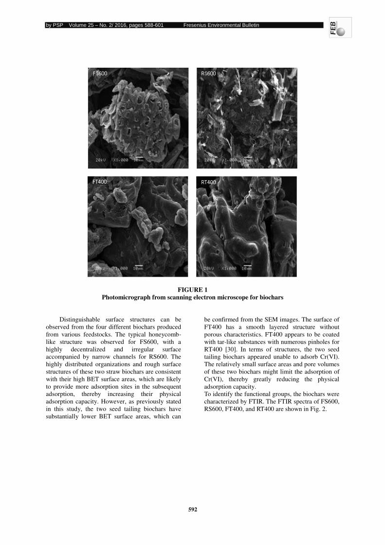
by PSP Volume 25 – No. 2/ 2016, pages 588-601 Fresenius Environmental Bulletin
592
FIGURE 1
Photomicrograph from scanning electron microscope for biochars
Distinguishable surface structures can be
observed from the four different biochars produced
from various feedstocks. The typical honeycomb-
like structure was observed for FS600, with a
highly decentralized and irregular surface
accompanied by narrow channels for RS600. The
highly distributed organizations and rough surface
structures of these two straw biochars are consistent
with their high BET surface areas, which are likely
to provide more adsorption sites in the subsequent
adsorption, thereby increasing their physical
adsorption capacity. However, as previously stated
in this study, the two seed tailing biochars have
substantially lower BET surface areas, which can
be confirmed from the SEM images. The surface of
FT400 has a smooth layered structure without
porous characteristics. FT400 appears to be coated
with tar-like substances with numerous pinholes for
RT400 [30]. In terms of structures, the two seed
tailing biochars appeared unable to adsorb Cr(VI).
The relatively small surface areas and pore volumes
of these two biochars might limit the adsorption of
Cr(VI), thereby greatly reducing the physical
adsorption capacity.
To identify the functional groups, the biochars were
characterized by FTIR. The FTIR spectra of FS600,
RS600, FT400, and RT400 are shown in Fig. 2.
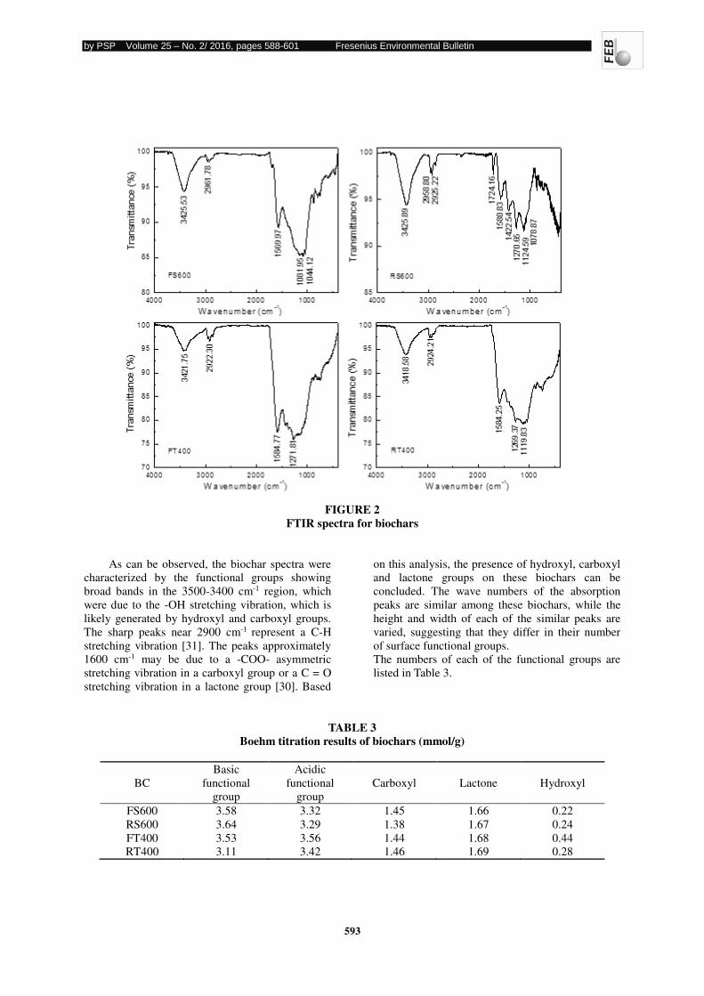
by PSP Volume 25 – No. 2/ 2016, pages 588-601 Fresenius Environmental Bulletin
593
FIGURE 2
FTIR spectra for biochars
As can be observed, the biochar spectra were
characterized by the functional groups showing
broad bands in the 3500-3400 cm-1 region, which
were due to the -OH stretching vibration, which is
likely generated by hydroxyl and carboxyl groups.
The sharp peaks near 2900 cm-1 represent a C-H
stretching vibration [31]. The peaks approximately
1600 cm-1 may be due to a -COO- asymmetric
stretching vibration in a carboxyl group or a C = O
stretching vibration in a lactone group [30]. Based
on this analysis, the presence of hydroxyl, carboxyl
and lactone groups on these biochars can be
concluded. The wave numbers of the absorption
peaks are similar among these biochars, while the
height and width of each of the similar peaks are
varied, suggesting that they differ in their number
of surface functional groups.
The numbers of each of the functional groups are
listed in Table 3.
TABLE 3
Boehm titration results of biochars (mmol/g)
BC
Basic
functional
group
Acidic
functional
group
Carboxyl Lactone Hydroxyl
FS600 3.58 3.32 1.45 1.66 0.22
RS600 3.64 3.29 1.38 1.67 0.24
FT400 3.53 3.56 1.44 1.68 0.44
RT400 3.11 3.42 1.46 1.69 0.28
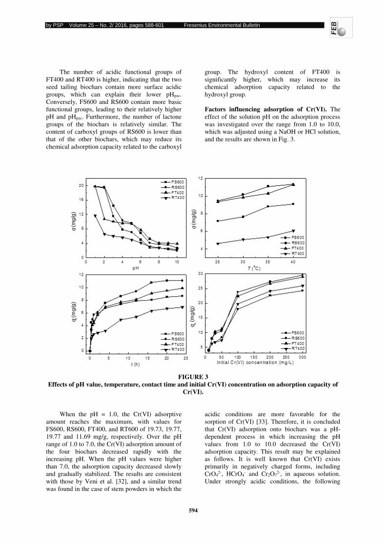
by PSP Volume 25 – No. 2/ 2016, pages 588-601 Fresenius Environmental Bulletin
594
The number of acidic functional groups of
FT400 and RT400 is higher, indicating that the two
seed tailing biochars contain more surface acidic
groups, which can explain their lower pHpzc.
Conversely, FS600 and RS600 contain more basic
functional groups, leading to their relatively higher
pH and pHpzc. Furthermore, the number of lactone
groups of the biochars is relatively similar. The
content of carboxyl groups of RS600 is lower than
that of the other biochars, which may reduce its
chemical adsorption capacity related to the carboxyl
group. The hydroxyl content of FT400 is
significantly higher, which may increase its
chemical adsorption capacity related to the
hydroxyl group.
Factors influencing adsorption of Cr(VI). The
effect of the solution pH on the adsorption process
was investigated over the range from 1.0 to 10.0,
which was adjusted using a NaOH or HCl solution,
and the results are shown in Fig. 3.
FIGURE 3
Effects of pH value, temperature, contact time and initial Cr(VI) concentration on adsorption capacity of
Cr(VI).
When the pH = 1.0, the Cr(VI) adsorptive
amount reaches the maximum, with values for
FS600, RS600, FT400, and RT600 of 19.73, 19.77,
19.77 and 11.69 mg/g, respectively. Over the pH
range of 1.0 to 7.0, the Cr(VI) adsorption amount of
the four biochars decreased rapidly with the
increasing pH. When the pH values were higher
than 7.0, the adsorption capacity decreased slowly
and gradually stabilized. The results are consistent
with those by Veni et al. [32], and a similar trend
was found in the case of stem powders in which the
acidic conditions are more favorable for the
sorption of Cr(VI) [33]. Therefore, it is concluded
that Cr(VI) adsorption onto biochars was a pH-
dependent process in which increasing the pH
values from 1.0 to 10.0 decreased the Cr(VI)
adsorption capacity. This result may be explained
as follows. It is well known that Cr(VI) exists
primarily in negatively charged forms, including
CrO42-, HCrO4
- and Cr2O72-, in aqueous solution.
Under strongly acidic conditions, the following
by PSP Volume 25 – No. 2/ 2016, pages 588-601 Fresenius Environmental Bulletin
595
changes may occur in a biochar-Cr(VI) solution
system [34]:
2CrO42- + 2H+ ↔ Cr2O7
2- + H2O (2)
R-C=O + Cr2O72- + H+ → R-C=O…HOCr2O5
-
(Hydrogen bonds) (3)
R-C=O + HCrO4- → R-C=O…HOCrO3
- (Hydrogen
bonds) (4)
Under the participation of H+, an abundance of
C=O groups on the biochar surface can bind with
the anions forming hydrogen bonds, resulting in an
increased amount of Cr(VI) adsorbed onto the
biochars; hence, the Cr(VI) adsorption capacity
increased. In addition, a protonated functional
group, such as -OH, is positively charged, which
enhances the adsorption of negatively charged
Cr(VI) anions by electrostatic binding [35]. This
result could be illustrated by the sharp increase of
the adsorptive amount of Cr(VI) by FS600 and
RS600 when the pH values were less than their
pHZPC (4.73 and 5.08, respectively) and those by
FT400 and RT400 when the pH values were less
than their pHZPC (3.06 and 2.84, respectively). In
addition, an excess of OH- could effectively
compete with the Cr(VI) ions for the bonding sites
when the pH value was increased [36], leading to a
relatively lower Cr(VI) adsorption capacity. The
conversion of a portion of Cr(VI) into Cr(III) in a
substantially more acidic solution was
demonstrated [17-19]. In the present study, the
conversions were also found when the pH values of
the solution were less than 2. However, the
conversions were negligible when the pH values of
the solution were higher than 3.
Temperature is a critical factor for adsorption
processes. The adsorption capacity of Cr(VI) was
investigated at various temperatures. The results are
shown in Fig 3. As the temperature increased from
25 °C to 40 °C, the amount of Cr(VI) adsorbed onto
FS600, RS600, FT400 and RT400 increased from
7.08, 9.48, 9.57, 4.61 mg/g to 9.08, 11.34, 11.29,
6.06 mg/g, respectively. Higher temperatures
favored a slight but statistically significant increase
in Cr(VI) adsorption onto these biochars, indicating
that the adsorption was a chemisorption and was a
thermodynamically favorable endothermic process
[27]. These results are consistent with a previous
report [37] in which Cr(VI) uptake increased with
increasing temperature for clay over the range of
303-313 K. The results are also consistent with the
work of Chen et al., who suggested that increased
temperatures supplied sufficient energy to the
heavy metal ions to overcome the diffuse double
layer and to adsorb onto the interior structure of the
biochars [27]. It is well known that an increase in
temperature causes the molecules to move at a
greater speed and with less interaction time; thus,
more Cr(VI) ions were able to overcome the
adsorption activation energy barrier and attach to
the biochar surface [37]. Although a high
temperature is advantageous to improve the
adsorption capacity, when considering the
convenience of the actual operation, the following
experiments should be performed at 25 °C.
The effect of contact time on adsorption was
investigated over the range from 0 to 24 h for each
biochar, and the results are shown in Fig. 3. The
Cr(VI) adsorption capacity increases with
increasing contact time. The adsorption process
could be divided into three stages: a rapid initial
rate followed by a substantially slower adsorption
rate and then equilibrium. In the first 4 h, the
adsorption rate increased rapidly, followed by a
slow approach to equilibrium. There was no
significant difference in the sorption amount
between 20 h and 24 h. Therefore, 24 h was taken
as the equilibration time for the adsorption of
Cr(VI) onto the biochars. Of the biochar
adsorbents, RS600 shows the highest adsorption
performance for Cr(VI), followed by FT400, FS600
and RT400, over the tested range. Initially, active
binding sites were highly available on the biochar
surfaces; consequently, the adsorption process onto
the sorbents was easy and rapid. However, with
increasing coverage, the fraction of the surface
rapidly diminished, and chromium ions had to
compete among themselves for the adsorption sites,
causing the absorbance on the surface of the
biochar to be substantially more difficult and slow
[29].
The sorption of Cr(VI) ions was tested at
different initial Cr(VI) concentrations ranging from
10-300 mg/L (Fig. 3). Increasing the concentration
leads to an increase of the adsorption capacity of
Cr(VI) by the biochars. At a lower concentration
(<100 mg/L), the Cr(VI) adsorption capacity
increases rapidly, possibly because all of the Cr(VI)
ions in the solution would react with the binding
sites, thus facilitating nearly complete adsorption.
At a higher concentration (>100 mg/L), a smooth
growth would occur in the adsorption capacity
because more Cr(VI) ions remain unsorbed in the
solution due to saturation of the binding sites [35].
It was also observed that the adsorption capacity
increases exponentially with high concentrations,
which is consistent with the findings by Ozer et al.
[35], who indicated that mass transfer limitations
were overcome by the high driving force of the
concentration difference between the liquid and
solid phases.
by PSP Volume 25 – No. 2/ 2016, pages 588-601 Fresenius Environmental Bulletin
596
As illustrated above, given the pH value (4 ~
5), temperature (25 °C), contact time, and the initial
concentration of Cr (VI) (50 mg/L), the adsorptive
capacities of Cr(VI) onto biochars are in the order
of RS600 > FT400 > FS600 > RT400. This result is
not consistent with the BET surface areas of
biochars, which are in the order of RS600 > FS600
>> RT400 > FT400 (Table 2). It could be deduced
that a chemical reaction occurred in the adsorption
process.
Adsorption kinetics. To examine the
controlling mechanism for the adsorption process,
pseudo-first-order and pseudo-second-order models
are used to simulate collected data of the sorption
kinetics. The first-order rate equation can be
represented as follows:
tkqqq ete 1ln)(ln (5)
Similarly, the second-order rate equation is
given by:
eet q
t
qkq
t
2
2
1 (6)
where qt (mg/g) and qe (mg/g) are the amounts of
Cr(VI) sorbed at time t and at equilibrium,
respectively; and k1 and k2 are the first-order and
second-order apparent sorption rate constants,
respectively. The plot of ln(qe-qt)-t should yield a
linear relationship, from which k1 and qe can be
determined from the slope and the intercept of the
plot, respectively. The linear plots of t/qt - t can give
the pseudo-second-order adsorption rate constant k2
from the slope, and qe can be calculated from the
intercept [37]. The results based on the adsorption
capacity of Cr(VI) are summarized in Table 4.
TABLE 4
Kinetic parameters of adsorption of Cr(VI) onto biochars
BC qe,ex
(mg/g)
Pseudo-first-order model Pseudo-second-order model
qe,cal
(mg/g)
k1
(1/h) R2
qe,cal
(mg/g)
k2
(g/mg h) R2
FS600 8.64 4.83 0.156 0.9573 8.71 0.137 0.9970
RS600 11.1 9.08 0.229 0.9282 11.40 0.0715 0.9902
FT400 9.52 6.52 0.134 0.9655 9.96 0.0801 0.9904
RT400 6.90 5.69 0.143 0.9676 7.18 0.0630 0.9698
The results show that the correlation
coefficients of each biochar were higher (R2 >
0.9698) for the pseudo-second-order model than for
the pseudo-first-order model. The differences
between the measured maximum adsorptive amount
(qe, ex) and the calculated amount (qe, cal) suggest that
the sorption kinetics of Cr(VI) onto biochars fitted well into the pseudo-second-order kinetics model,
indicating that chemisorption might have been the
major sorption mechanism [26]. It was also
confirmed by the observation that chemisorption
was the rate-limiting mechanism for the adsorption
of chromium onto biochars. Similar observations
have been reported by Jia et al., who studied
oxytetracycline sorption onto maize-straw-derived
biochar [26].
Adsorption isotherms. Adsorption isotherms
express the relationship between the amount of
adsorbed Cr(VI) per unit mass of each biochar (qe)
and the Cr(VI) concentration in solution (ce) at
equilibrium. Of several isotherm equations, the two
most commonly used, the Langmuir and Freundlich
adsorption isotherms, were investigated in this
study. The Langmuir equation, as follows, suggests
that the monolayer sorption onto a surface contains
a finite number of identical sites:
mm
e
e
e
bqq
c
q
c 1 (7)
The empirical Freundlich equation based on
sorption on a heterogeneous surface is given by the
following equation:
eFe cn
Kq ln1
lnln (8)
where ce (mg/L) and qe (mg/g) show the
residual Cr(VI) concentration and the amount of
Cr(VI) adsorbed on the biochars at equilibrium,
respectively; b is the Langmuir constant related to
the energy of adsorption; qm is the maximum
adsorption capacity of the biochars; and KF and n
are the Freundlich constants, which are the
indicators of the adsorption capacity and adsorption
intensity, respectively.
Based on the plots of ce/qe versus ce, the constants
qm and b were calculated from the slope and
intercept of the graph, respectively, KF can be
determined from the intercept value, and n can be
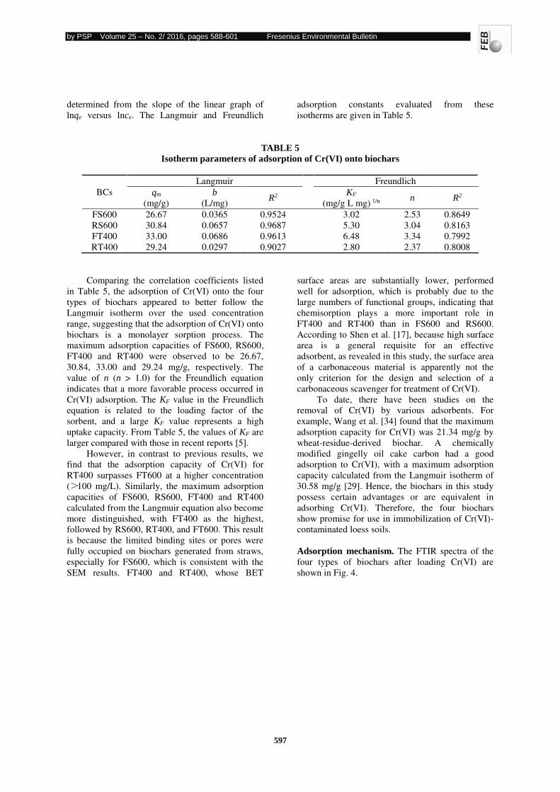
by PSP Volume 25 – No. 2/ 2016, pages 588-601 Fresenius Environmental Bulletin
597
determined from the slope of the linear graph of
lnqe versus lnce. The Langmuir and Freundlich
adsorption constants evaluated from these
isotherms are given in Table 5.
TABLE 5
Isotherm parameters of adsorption of Cr(VI) onto biochars
BCs
Langmuir Freundlich
qm
(mg/g)
b
(L/mg) R2
KF
(mg/g L mg) 1/n n R2
FS600 26.67 0.0365 0.9524 3.02 2.53 0.8649
RS600 30.84 0.0657 0.9687 5.30 3.04 0.8163
FT400 33.00 0.0686 0.9613 6.48 3.34 0.7992
RT400 29.24 0.0297 0.9027 2.80 2.37 0.8008
Comparing the correlation coefficients listed
in Table 5, the adsorption of Cr(VI) onto the four
types of biochars appeared to better follow the
Langmuir isotherm over the used concentration
range, suggesting that the adsorption of Cr(VI) onto
biochars is a monolayer sorption process. The
maximum adsorption capacities of FS600, RS600,
FT400 and RT400 were observed to be 26.67,
30.84, 33.00 and 29.24 mg/g, respectively. The
value of n (n > 1.0) for the Freundlich equation
indicates that a more favorable process occurred in
Cr(VI) adsorption. The KF value in the Freundlich
equation is related to the loading factor of the
sorbent, and a large KF value represents a high
uptake capacity. From Table 5, the values of KF are
larger compared with those in recent reports [5].
However, in contrast to previous results, we
find that the adsorption capacity of Cr(VI) for
RT400 surpasses FT600 at a higher concentration
(>100 mg/L). Similarly, the maximum adsorption
capacities of FS600, RS600, FT400 and RT400
calculated from the Langmuir equation also become
more distinguished, with FT400 as the highest,
followed by RS600, RT400, and FT600. This result
is because the limited binding sites or pores were
fully occupied on biochars generated from straws,
especially for FS600, which is consistent with the
SEM results. FT400 and RT400, whose BET
surface areas are substantially lower, performed
well for adsorption, which is probably due to the
large numbers of functional groups, indicating that
chemisorption plays a more important role in
FT400 and RT400 than in FS600 and RS600.
According to Shen et al. [17], because high surface
area is a general requisite for an effective
adsorbent, as revealed in this study, the surface area
of a carbonaceous material is apparently not the
only criterion for the design and selection of a
carbonaceous scavenger for treatment of Cr(VI).
To date, there have been studies on the
removal of Cr(VI) by various adsorbents. For
example, Wang et al. [34] found that the maximum
adsorption capacity for Cr(VI) was 21.34 mg/g by
wheat-residue-derived biochar. A chemically
modified gingelly oil cake carbon had a good
adsorption to Cr(VI), with a maximum adsorption
capacity calculated from the Langmuir isotherm of
30.58 mg/g [29]. Hence, the biochars in this study
possess certain advantages or are equivalent in
adsorbing Cr(VI). Therefore, the four biochars
show promise for use in immobilization of Cr(VI)-
contaminated loess soils.
Adsorption mechanism. The FTIR spectra of the
four types of biochars after loading Cr(VI) are
shown in Fig. 4.
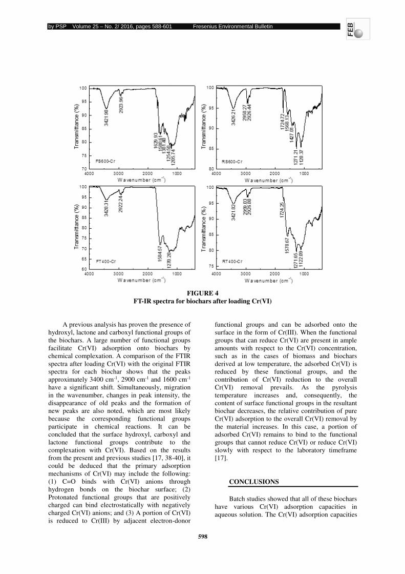
by PSP Volume 25 – No. 2/ 2016, pages 588-601 Fresenius Environmental Bulletin
598
FIGURE 4
FT-IR spectra for biochars after loading Cr(VI)
A previous analysis has proven the presence of
hydroxyl, lactone and carboxyl functional groups of
the biochars. A large number of functional groups
facilitate Cr(VI) adsorption onto biochars by
chemical complexation. A comparison of the FTIR
spectra after loading Cr(VI) with the original FTIR
spectra for each biochar shows that the peaks
approximately 3400 cm-1, 2900 cm-1 and 1600 cm-1
have a significant shift. Simultaneously, migration
in the wavenumber, changes in peak intensity, the
disappearance of old peaks and the formation of
new peaks are also noted, which are most likely
because the corresponding functional groups
participate in chemical reactions. It can be
concluded that the surface hydroxyl, carboxyl and
lactone functional groups contribute to the
complexation with Cr(VI). Based on the results
from the present and previous studies [17, 38-40], it
could be deduced that the primary adsorption
mechanisms of Cr(VI) may include the following:
(1) C=O binds with Cr(VI) anions through
hydrogen bonds on the biochar surface; (2)
Protonated functional groups that are positively
charged can bind electrostatically with negatively
charged Cr(VI) anions; and (3) A portion of Cr(VI)
is reduced to Cr(III) by adjacent electron-donor
functional groups and can be adsorbed onto the
surface in the form of Cr(III). When the functional
groups that can reduce Cr(VI) are present in ample
amounts with respect to the Cr(VI) concentration,
such as in the cases of biomass and biochars
derived at low temperature, the adsorbed Cr(VI) is
reduced by these functional groups, and the
contribution of Cr(VI) reduction to the overall
Cr(VI) removal prevails. As the pyrolysis
temperature increases and, consequently, the
content of surface functional groups in the resultant
biochar decreases, the relative contribution of pure
Cr(VI) adsorption to the overall Cr(VI) removal by
the material increases. In this case, a portion of
adsorbed Cr(VI) remains to bind to the functional
groups that cannot reduce Cr(VI) or reduce Cr(VI)
slowly with respect to the laboratory timeframe
[17].
CONCLUSIONS
Batch studies showed that all of these biochars
have various Cr(VI) adsorption capacities in
aqueous solution. The Cr(VI) adsorption capacities
by PSP Volume 25 – No. 2/ 2016, pages 588-601 Fresenius Environmental Bulletin
599
of FS600, RS600, FT400 and RT400 are 7.27,
10.07, 9.49 and 5.65 mg/g, respectively, at pH 4.8
and at 25 °C, with a biochar dose of 0.05 g and an
initial Cr(VI) content of 50 mg/L. Thus, RS600
provides the best remediation for contaminated soil,
followed by FT400, FS600 and RT400. The
adsorption of Cr(VI) onto these biochars follows
pseudo-second-order kinetics. The isotherm
adsorption of Cr(VI) onto biochars fitted well into the Langmuir isothermal model, and the maximum
adsorption capacities of Cr(VI) were found to be
26.67, 30.84, 33.00 and 29.24 mg/g for LS600,
BS600, LO400 and BO400, respectively. It is also
concluded that the mechanisms of Cr(VI)
adsorption onto biochars primarily include
chemical bonds and electrostatic attraction.
ACKNOWLEDGEMENTS
This paper was financially supported by the
National Natural Science Foundation of China
(21167007, 21467013), the Specialized Research
Fund for the Doctoral Program of Higher Education
of China (20136204110003) and the Youth Science
Foundation of Lanzhou Jiaotong University
(2013015).
REFERENCES
[1] Shen, Y., Li, L., Chen, W., Robertson, M.,
Unkovich, M., Bellotti, W. and Probert, M.
(2009) Soil water, soil nitrogen and
productivity of lucerne-wheat sequences on
deep silt loams in a summer dominant rainfall
environment. Field Crops Res. 111, 97-108.
[2] Liu, J., Cao, J., Nan, Z. R., Wang, S. L., Hu, X.
N. and Chen, J. S. (2010) Impact of heavy
metal combined pollution on soil enzyme
activity in Baiyin region, Gansu province. J.
Lanzhou Univ. 46, 39-43.
[3] Zhao, B. W. and Wang, G. (2010) Preliminary
investigation and assessment of farmland soils
contaminated by heavy metal around Baiyin
City. Environ. Sci. Technol. 33, 79-81, 105.
[4] Lehmann, J. (2007) A handful of carbon.
Nature. 447, 143-144.
[5] Agrafioti, E., Kalderis, D. and Diamadopoulos,
E. (2014) Arsenic and chromium removal
from water using biochars derived from rice
husk, organic solid wastes and sewage sludge.
J. Environ. Manage. 133, 309-314.
[6] Steiner, C., Glaser, B., Teixeira, W. G.,
Lehmann, J., Blum, W. E. H. and Zech, W.
(2008) Nitrogen retention and plant uptake on
a highly weathered central Amazonian
ferralsol amended with compost and charcoal.
J. Plant Nut. Soil Sci. 171, 893-899.
[7] Glaser, B., Lehman, J. and Zech, W. (2002)
Ameliorating physical and chemical properties
of highly weathered soils in the tropics with
charcoal. Biol. Fert. Soils. 35, 219-230.
[8] Ladygina, N. and Rinceau, F. (2013) Biochar
and Soil Biota. CRC Press, New York.
[9] Lehmann, J. and Joseph, S. (2009) Biochar for
Environmental Management: Science and
Technology. Earthscan, London.
[10] Costa, M. (2003) Potential hazards of
hexavalent chromate in our drinking water.
Toxicol. Appl. Pharmacol. 188, 1-5.
[11] Sun, W., Shen, W., Wang, Q., Ding, S. and
Su, S. (2013) Adsorption of chromium (Ⅵ)
from aqueous solution onto aluminum pillared
pyrolusite leaching residue. Fresen. Environ.
Bull. 22, 2645-2650.
[12] Yari, A. R., Nasseri, S., Mahvi, A. H.,
Nabizadeh, R., Kalantari, R. R. and Yunesian,
M. (2013) Application of a forward osmosis
membrane in removal of chromium from
aqueous solutions. Fresen. Environ. Bull. 22,
2319-2323.
[13] Beltran-Prieto, J. C., Kolomaznfk, K. and
Veloz-Rodriguez, R. (2013) Removal of
chromium from tannery wastewater using
waste-building material. Fresen. Environ.
Bull. 22, 573-578.
[14] Ghaneian, M. T., Ghanizadeh, G., Asgari, G.
and Mohammadi, A. M. S. (2012) Kinetics
and isotherm studies of hexavalent chromium
adsorption from water using bone charcoal.
Fresen. Environ. Bull. 21, 1296-1302.
[15] Netzahuatl-Munoz, A. R., Aranda-Garcia, E.,
Cristiani-Urbina, M. C., Barragan-Huerta, B.
E., Villegas-Garrido, T. L. and Cristiani-
Urbina, E. (2010) Removal of hexavalent and
total chromium from aqueous solutions by
schinus molle bark. Fresen. Environ. Bull. 19,
2911-2918.
[16] Yi, X. (2004) Study on purification of loessial
soil to Cr(VI) and its migration characters. J.
Soil Water Conserv. 18, 24-27, 23.
[17] Shen, Y. S., Wang, S. L., Tzou, Y. M., Yan,
Y. Y. and Kuan, W. H. (2012) Removal of
hexavalent Cr by coconut coir and derived
chars: The effect of surface functionality.
Bioresource Technol. 104, 165-172.
[18] Zhang, W., Mao, S., Chen, H., Huang, L. and
Qiu, R. (2013) Pb(II) and Cr(VI) sorption by
biochars pyrolyzed from the municipal
wastewater sludge under different heating
conditions. Bioresource Technol. 147, 545-
552.
[19] Dong, X., Ma, L. Q. and Li, Y. (2011)
by PSP Volume 25 – No. 2/ 2016, pages 588-601 Fresenius Environmental Bulletin
600
Characteristics and mechanisms of hexavalent
chromium removal by biochar from sugar beet
tailing. J. Hazard. Mater. 190, 909-915.
[20] Abdel-Fattah, T. M., Mahmoud, M. E.,
Ahmed, S. B., Huff, M. D., Lee, J. W. and
Kumar, S. (2015) Biochar from woody
biomass for removing metal contaminants and
carbon sequestration. J. Ind. Eng. Chem. 22,
103-109.
[21] Zhao, B. and Nartey, O. D. (2014)
Characterization and evaluation of biochars
derived from agricultural waste biomasses
from Gansu, China. Proceedings of the 2014
World Congress on Advances in Civil,
Environmental, and Materials Research.
Techno-Press, Busan.
[22] Liu, F. and Liu, X. (2007) Monitoring and
Analysis Technology for Soils and Waste
Solids. Chemical Industry Press, Beijing.
[23] Boehm, H. P. (1994) Some aspects of the
surface chemistry of carbon blacks and other
carbons. Carbon. 32, 759-769.
[24] China EPA. (2005) Monitoring and Analysis
Methods for water and Waste Water (4th Ed.).
China Environment Press, Beijing.
[25] Song, W. and Guo, M. (2012) Quality
variations of poultry litter BC generated at
different pyrolysis temperatures. J. Anal. App.
Pyrol. 94, 138-145.
[26] Jia, M., Wang, F., Bian, Y., Jin, X., Kengara,
F. O. and Xu, R. (2013) Effects of pH and
metal ions on oxytetracycline sorption to
maize-straw-derived biochar. Bioresource
Technol. 136, 87-93.
[27] Chen, X., Chen, G., Chen, L., Chen, Y.,
Lehmann, J., Mcbridge, M. B. and Hay, A. G.
(2011) Adsorption of copper and zinc by
biochars produced from pyrolysis of
hardwood and corn straw in aqueous solution.
Bioresource Technol. 102, 8877-8884.
[28] Sun, K., Ro, K., Guo, M., Navok, J.,
Mashayekhi, H. and Xin, B. (2011) Sorption
of bisphenol A, 17α-ethinyl estradiol and
phenanthrene on thermally and
hydrothermally produced biochars.
Bioresource Technol. 102, 5757-5763.
[29] Nagashanmugam, K. B. and Srinivason, K.
(2011) Removal of chromium (VI) from
aqueous solution by chemically modified
gingelly oil cake carbon. Indian J. Chem.
Technol. 18, 207-219.
[30] Regmi, P., Moscoso, J. L. G., Kumar, S., Cao,
X. and Mao, J. (2012) Removal of copper and
cadmium from aqueous solution using
switchgrass biochar produced via
hydrothermal carbonization process. J.
Environ. Manage. 109, 61-69.
[31] Singh, S. R. and Singh, A. P. (2012)
Treatment of water containg chromium (VI)
using rice husk carbon as a new low cost
adsorbent. Int. J. Environ. Res. 6, 917-924.
[32] Veni, V. K. and Ravindhranath, K. (2012)
Stems and their ashes of some herbal plants as
adsorbents in the removal of chromium (VI)
from waste waters. Int. J. App. Biol. Pharm.
Technol. 3, 151-166.
[33] Sen, A. U., Olivella, A., Fiol, N., Miranda, I.,
Villaescusa, I. and Pereira, H. (2012) Removal
of chromium(VI) in aqueous environments
using cork and heat-treated cork samples from
quercus cerris and quercus suber.
Bioresources. 7, 4843-4857.
[34] Wang, X. S., Chen, L. F., Li, F. Y., Chen, K.
L., Wan, W. Y. and Tang, Y. J. (2010)
Removal of Cr(VI) with wheat-residue
derived black carbon: reaction mechanism and
adsorption performance. J. Hazard. Mater.
175, 816-822.
[35] Ozer, T. B., Erkaya, I. A., Udoh, A. U.,
Duygu, D. Y., Akbulut, A., Bayramoglu, G.
and Arica, M. Y. (2012) Biosorption of Cr(VI)
by free and immobilized pediastrum
boryanum biomass: equilibrium, kinetic, and
thermodynamic studies. Environ. Sci. Pollut.
Res. 19, 2983-2993.
[36] Wang, W., Li, M. and Zeng, Q. (2012)
Column adsorption of chromium (VI) by
strong alkaline anion-exchange fiber. J. App.
Poly. Sci. 126, 1733-1738.
[37] Bhattacharyya, K. G. and Gupta, S. S. (2006)
Adsorption of chromium (VI) from water by
clays. Ind. Eng. Chem. Res. 45, 7232-7240.
[38] Saha, B. and Orvig, C. (2010) Biosorbents for
hexavalent chromium elimination from
industrial and municipal effluents. Coordin.
Chem. Rev. 254, 2959-2972.
[39] Park, D. H., Lim, S. R., Yun, Y. S. and Park,
J. M. (2007) Reliable evidences that the
removal mechanism of hexavalent chromium
by natural biomaterials is adsorption coupled
reduction. Chemosphere. 70, 298-305.
[40] Park, D. H., Park, J. M. and Yun, Y. S. (2006)
Mechanisms of the removal of hexavalent
chromium by biomaterials or biomaterial-
based activated carbons. J. Hazard. Mater.
B137, 1254-1257.
Received: 04.08.2015
Accepted: 06.12.2015

by PSP Volume 25 – No. 2/ 2016, pages 588-601 Fresenius Environmental Bulletin
601
CORRESPONDING AUTHOR
Baowei Zhao Lanzhou Jiaotong University
School of Environmental and Municipal
Engineering
88 West Anning Rd.
Lanzhou 730070 - P. R. CHINA
e-mail: [email protected]
by PSP Volume 25 – No. 2/2016, pages 602-611 Fresenius Environmental Bulletin
602
REMEDIATION EFFECTS OF MAIZE-STRAW-DERIVED
BIOCHAR ON RICE GROWN IN CADMIUM-CONTAMINATED
SOIL IN NORTH CHINA
Weiming Zhang, Liqun Xiu, Wenfu Chen
Biochar Engineering Technology Research Center of Liaoning Province, Agronomy College of Shenyang Agricultural University, Shenyang, China
ABSTRACT
To assess biochar potential for cadmium
(Cd)-contaminated soil, a pot experiment was
conducted with samples of typical farmland soil from
Shenyang area(North China), which was contaminated
with cadmium due to sewage irrigation. Two
maize-straw-derived biochar concentrations(11250 and
22500 kg·hm-2) were tested. The results showed that the
biochar prepared with dry distillation of carbonization
technology under oxygen-deficient conditions and low
temperature(400-450 ℃ ) had appropriate structural
features and physical and chemical properties. The use
of such biochar reduced the available-Cd ions in the
contaminated soil, with a “passivation or inhibitory”
effect which displayed a variable time-dependent
response. The biochar led to soil pH changes during rice
growth(increase followed by a decrease). Furthermore,
the biochar significantly improved the soil organic
matter and available-nutrients(N, P, K), and indeed a
cumulative effect with time was observed. More
importantly, the biochar significantly reduced the
cadmium content in rice grains by an average of
33.01% compared to the control(CK), the treatment
with higher biochar concentration being more effective;
this indicates a decreased bio-availability of the
cadmium. These results suggest that
maize-straw-derived biochar is an effective remediation
material for Cd-contaminated soil, which has good
application potential for the environment.
KEYWORDS:
Biochar, Maize straw, Cadmium-contaminated soil, Rice
INTRODUCTION
With the rapid development of modern
industrialization and urbanization, the production of
sewage and wastes in cities increased, together with
pollution; the excessive use of pesticides and chemical
fertilizer, on the other hand, caused a gradual decline in
farmland quality [1]. Heavy metal pollution of farmland,
in particular, became one of the most important
problems for the government, experts and for the
public’s attention. According to statistics, which
probably underestimate the problem, China’s heavy
metal pollution of current farmland could be higher than
2×10⁷hm2, resulting in a reduction of crop production
up to 1×10⁷t [2]. Among the heavy metal pollutants,
cadmium is one of the most toxic and which can affect
the environment the most. Heavy metal pollution not
only reduces crop yield, but also threatens human health
through the “food-health” chain, becoming an
“invisible-killer” which can affect national grain
production, food safety and the overall sustainable
development of society. At present, the main methods
to deal with heavy metal pollution are precipitation,
complexation, irrigation, and antagonistic and
electro-chemical methods. All these technologies,
however, are generally expensive, take time to be
effective and pose ecological security risks. It is
therefore crucial to develop effective remediation
techniques for heavy metal polluted farmland; such
technologies have to be cheaper, and efficient from an
ecological point of view.
Biochar has several characteristics which make it
an ideal material for agricultural and environmental
protection; these include a rich micro-pore structure,
large specific surface area and strongly adsorption
ability [3, 4]. Therefore, the development of biochar
technology looks to be a promising method for heavy
metal pollution remediation [5]. At present, several
studies showed that biochar acted as an adsorbent for
heavy metal ions, chlorobenzene-based organic
pollutants and pesticide residues, thereby reducing the
pollutant concentrations and their bioavailability [6-11].
Until now, however, the researches on biochar for
heavy metal pollution remediation were performed
mainly at laboratory scale; not many relevant reports
are available on the use of biochar in contaminated
farmland.
In this paper, the maize-straw-derived biochar was
used as an external material added to the soil to study
its remediation effects on soils of rice farmlands
contaminated with cadmium. The effects on the
cadmium concentration on several parts of the plant
(stems, leaves and rice grains) were also studied. The
results can clarify the possible role biochar can have on
the remediation of heavy metal contaminated farmland.
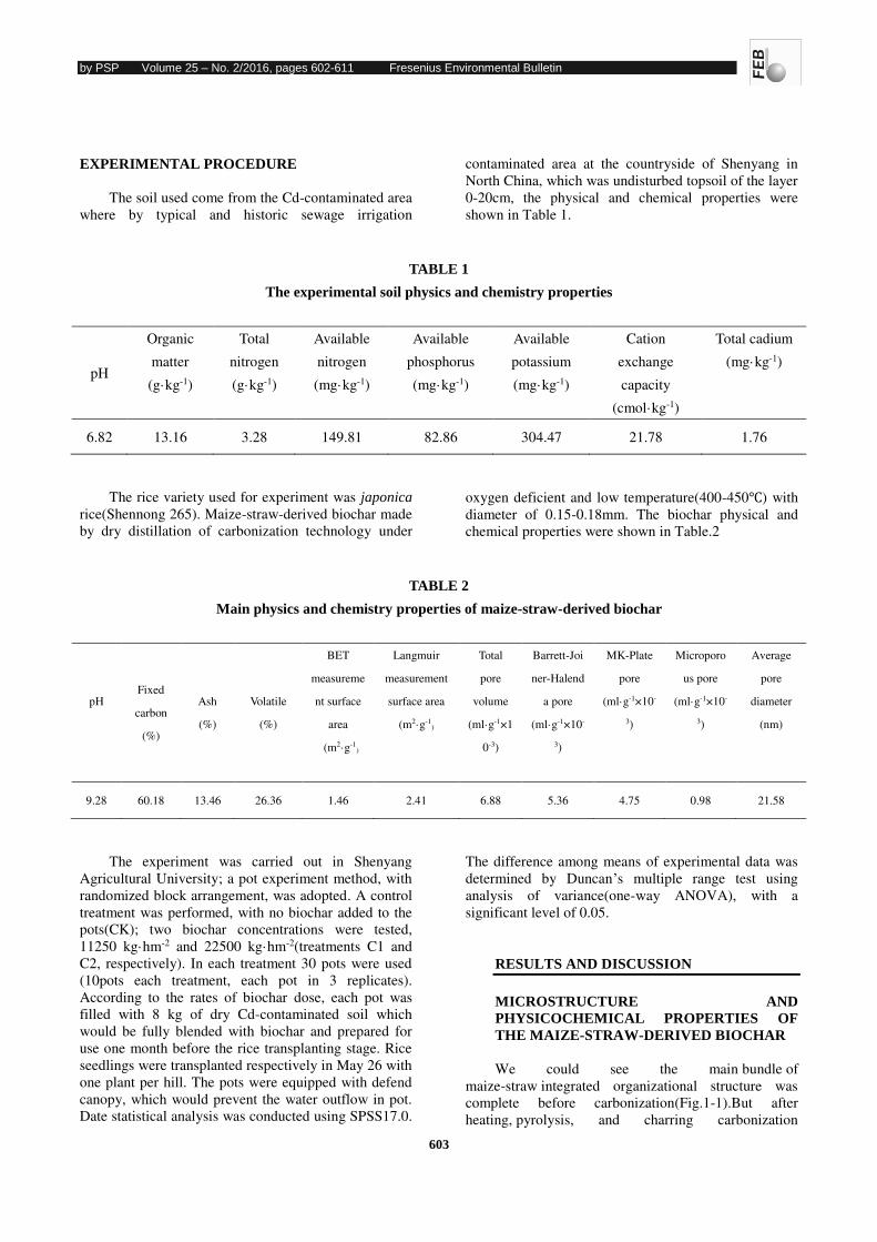
by PSP Volume 25 – No. 2/2016, pages 602-611 Fresenius Environmental Bulletin
603
EXPERIMENTAL PROCEDURE
The soil used come from the Cd-contaminated area
where by typical and historic sewage irrigation
contaminated area at the countryside of Shenyang in
North China, which was undisturbed topsoil of the layer
0-20cm, the physical and chemical properties were
shown in Table 1.
TABLE 1
The experimental soil physics and chemistry properties
pH
Organic
matter
(g·kg-1)
Total
nitrogen
(g·kg-1)
Available
nitrogen
(mg·kg-1)
Available
phosphorus
(mg·kg-1)
Available
potassium
(mg·kg-1)
Cation
exchange
capacity
(cmol·kg-1)
Total cadium
(mg·kg-1)
6.82 13.16 3.28 149.81 82.86 304.47 21.78 1.76
The rice variety used for experiment was japonica
rice(Shennong 265). Maize-straw-derived biochar made
by dry distillation of carbonization technology under
oxygen deficient and low temperature(400-450℃) with
diameter of 0.15-0.18mm. The biochar physical and
chemical properties were shown in Table.2
TABLE 2
Main physics and chemistry properties of maize-straw-derived biochar
pH
Fixed
carbon
(%)
Ash
(%)
Volatile
(%)
BET
measureme
nt surface
area
(m2·g-1)
Langmuir
measurement
surface area
(m2·g-1)
Total
pore
volume
(ml·g-1×1
0-3)
Barrett-Joi
ner-Halend
a pore
(ml·g-1×10-
3)
MK-Plate
pore
(ml·g-1×10-
3)
Microporo
us pore
(ml·g-1×10-
3)
Average
pore
diameter
(nm)
9.28 60.18 13.46 26.36 1.46 2.41 6.88 5.36 4.75 0.98 21.58
The experiment was carried out in Shenyang
Agricultural University; a pot experiment method, with
randomized block arrangement, was adopted. A control
treatment was performed, with no biochar added to the
pots(CK); two biochar concentrations were tested,
11250 kg·hm-2 and 22500 kg·hm-2(treatments C1 and
C2, respectively). In each treatment 30 pots were used
(10pots each treatment, each pot in 3 replicates).
According to the rates of biochar dose, each pot was
filled with 8 kg of dry Cd-contaminated soil which
would be fully blended with biochar and prepared for
use one month before the rice transplanting stage. Rice
seedlings were transplanted respectively in May 26 with
one plant per hill. The pots were equipped with defend
canopy, which would prevent the water outflow in pot.
Date statistical analysis was conducted using SPSS17.0.
The difference among means of experimental data was
determined by Duncan’s multiple range test using
analysis of variance(one-way ANOVA), with a
significant level of 0.05.
RESULTS AND DISCUSSION
MICROSTRUCTURE AND
PHYSICOCHEMICAL PROPERTIES OF
THE MAIZE-STRAW-DERIVED BIOCHAR
We could see the main bundle of
maize-straw integrated organizational structure was
complete before carbonization(Fig.1-1).But after
heating, pyrolysis, and charring carbonization
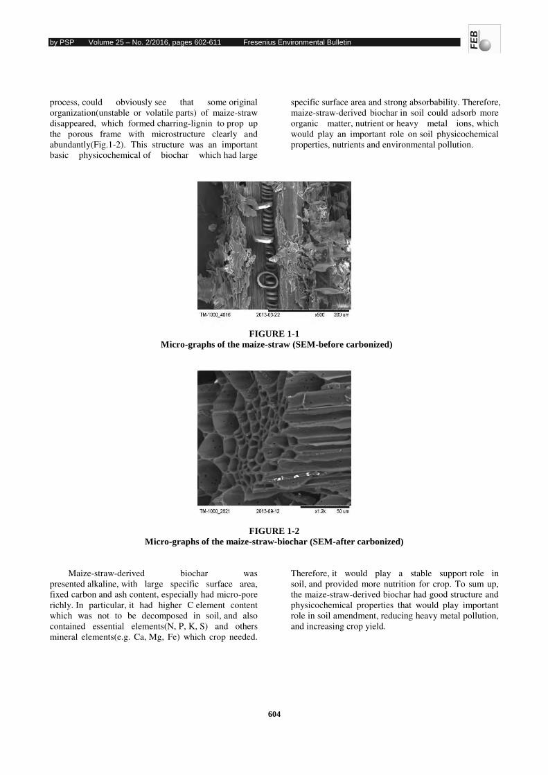
by PSP Volume 25 – No. 2/2016, pages 602-611 Fresenius Environmental Bulletin
604
process, could obviously see that some original
organization(unstable or volatile parts) of maize-straw
disappeared, which formed charring-lignin to prop up
the porous frame with microstructure clearly and
abundantly(Fig.1-2). This structure was an important
basic physicochemical of biochar which had large
specific surface area and strong absorbability. Therefore,
maize-straw-derived biochar in soil could adsorb more
organic matter, nutrient or heavy metal ions, which
would play an important role on soil physicochemical
properties, nutrients and environmental pollution.
FIGURE 1-1
Micro-graphs of the maize-straw (SEM-before carbonized)
FIGURE 1-2
Micro-graphs of the maize-straw-biochar (SEM-after carbonized)
Maize-straw-derived biochar was
presented alkaline, with large specific surface area,
fixed carbon and ash content, especially had micro-pore
richly. In particular, it had higher C element content
which was not to be decomposed in soil, and also
contained essential elements(N, P, K, S) and others
mineral elements(e.g. Ca, Mg, Fe) which crop needed.
Therefore, it would play a stable support role in
soil, and provided more nutrition for crop. To sum up,
the maize-straw-derived biochar had good structure and
physicochemical properties that would play important
role in soil amendment, reducing heavy metal pollution,
and increasing crop yield.
by PSP Volume 25 – No. 2/2016, pages 602-611 Fresenius Environmental Bulletin
605
TABLE 3
Main physics and chemistry properties of the maize-straw-derived biochar
pH
Fixed
carbon
(%)
Ash
(%)
Volatile
(%)
BET
surface area
(m2·g-1)
Total pore
volume
(ml·g-1×10⁻³)
Barrett-Joiner-
Halenda pore
(ml·g-1×10⁻³)
Microporous
pore
(ml·g-1×10⁻³)
Average
pore
diameter
(nm)
9.28 60.18 13.46 26.36 1.46 6.88 5.36 0.98 21.58
TABLE 4
Main elements composition of the maize-straw-derived biochar
Elements C N P K S Na Mg Ca Fe Al
Maize-straw-derived
biochar content
(%)
70.48 1.55 0.81 1.78 0.66 0.02 1.26 0.59 0.12 0.21
EFFECT OF MAIZE-STRAW-DERIVED
BIOCHAR ON pH OF
Cd-CONTAMINATION SOIL
Figure 2 shows the effect of biochar amendment
on the pH of the soil. It can be seen that such
differences were not significant at the rice tillering stage.
At the jointing stage, however, the pH of the soil for the
C2 treatment increased significantly in comparison with
other treatments, indicating the effectiveness of the
higher rate of biochar amendment. For the heading
stage, the pH of the soil of biochar treatments decreased
compared to the control, following the order
C2<C1<CK, with no significant difference between C1
and C2. Reaching the filling stage, the pH for the pots
with biochar treatments increased again, becoming
comparable with the control experiment. In general, the
soil pH of biochar amendment showed different values
in each rice growth period, with a wave-shaped trend;
this indicates a clear effect of the biochar, different in
each stage of the rice growth. The control, on the other
hand, was relatively stable, with no significant
fluctuations.
The biochar was alkaline, so its application into
the soil could have a direct effect on soil pH. This was
indeed observed in the early stage of rice growth; these
results are consistent with what was reported by Glaser,
et al. [12]. For the other stages, the changes in the pH of
the soil did not show a continuous increasing or
decreasing trend, as at first it became higher and then
lower. This may be related to the biochar adsorption by
different organic substances and base cations, which
changed the amount of cationic soil and its “activity
degree”. The biochar surface active sites may also
generate competitive adsorption with organic matter
and base cations; the adsorbed amount being related to
the different soil ecological environments, which led to
fluctuations in soil pH.
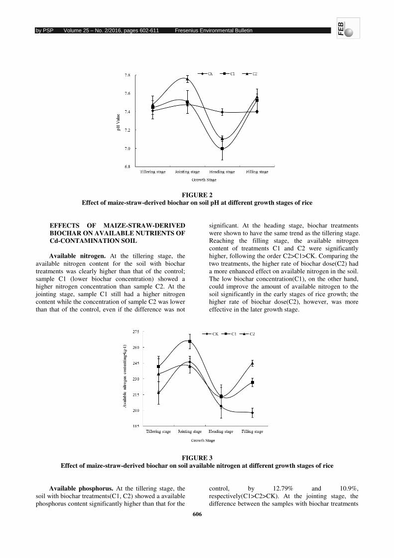
by PSP Volume 25 – No. 2/2016, pages 602-611 Fresenius Environmental Bulletin
606
FIGURE 2
Effect of maize-straw-derived biochar on soil pH at different growth stages of rice
EFFECTS OF MAIZE-STRAW-DERIVED
BIOCHAR ON AVAILABLE NUTRIENTS OF
Cd-CONTAMINATION SOIL
Available nitrogen. At the tillering stage, the
available nitrogen content for the soil with biochar
treatments was clearly higher than that of the control;
sample C1 (lower biochar concentration) showed a
higher nitrogen concentration than sample C2. At the
jointing stage, sample C1 still had a higher nitrogen
content while the concentration of sample C2 was lower
than that of the control, even if the difference was not
significant. At the heading stage, biochar treatments
were shown to have the same trend as the tillering stage.
Reaching the filling stage, the available nitrogen
content of treatments C1 and C2 were significantly
higher, following the order C2>C1>CK. Comparing the
two treatments, the higher rate of biochar dose(C2) had
a more enhanced effect on available nitrogen in the soil.
The low biochar concentration(C1), on the other hand,
could improve the amount of available nitrogen to the
soil significantly in the early stages of rice growth; the
higher rate of biochar dose(C2), however, was more
effective in the later growth stage.
FIGURE 3
Effect of maize-straw-derived biochar on soil available nitrogen at different growth stages of rice
Available phosphorus. At the tillering stage, the
soil with biochar treatments(C1, C2) showed a available
phosphorus content significantly higher than that for the
control, by 12.79% and 10.9%,
respectively(C1>C2>CK). At the jointing stage, the
difference between the samples with biochar treatments
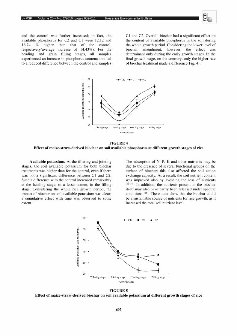
by PSP Volume 25 – No. 2/2016, pages 602-611 Fresenius Environmental Bulletin
607
and the control was further increased; in fact, the
available phosphorus for C2 and C1 were 12.12 and
16.74 % higher than that of the control,
respectively(average increase of 14.43%). For the
heading and grain filling stages, all samples
experienced an increase in phosphorus content; this led
to a reduced difference between the control and samples
C1 and C2. Overall, biochar had a significant effect on
the content of available phosphorus in the soil during
the whole growth period. Considering the lower level of
biochar amendment, however, the effect was
determinant only during the early growth stages. In the
final growth stage, on the contrary, only the higher rate
of biochar treatment made a difference(Fig. 4).
FIGURE 4
Effect of maize-straw-derived biochar on soil available phosphorus at different growth stages of rice
Available potassium. At the tillering and jointing
stages, the soil available potassium for both biochar
treatments was higher than for the control, even if there
was not a significant difference between C1 and C2.
Such a difference with the control increased remarkably
at the heading stage, to a lesser extent, in the filling
stage. Considering the whole rice growth period, the
impact of biochar on soil available potassium was clear;
a cumulative effect with time was observed to some
extent.
The adsorption of N, P, K and other nutrients may be
due to the presence of several functional groups on the
surface of biochar; this also affected the soil cation
exchange capacity. As a result, the soil nutrient content
was improved also by avoiding the loss of nutrients [13-14]. In addition, the nutrients present in the biochar
itself may also have partly been released under specific
conditions [15]. These data show that the biochar could
be a sustainable source of nutrients for rice growth, as it
increased the total soil nutrient level.
FIGURE 5
Effect of maize-straw-derived biochar on soil available potassium at different growth stages of rice
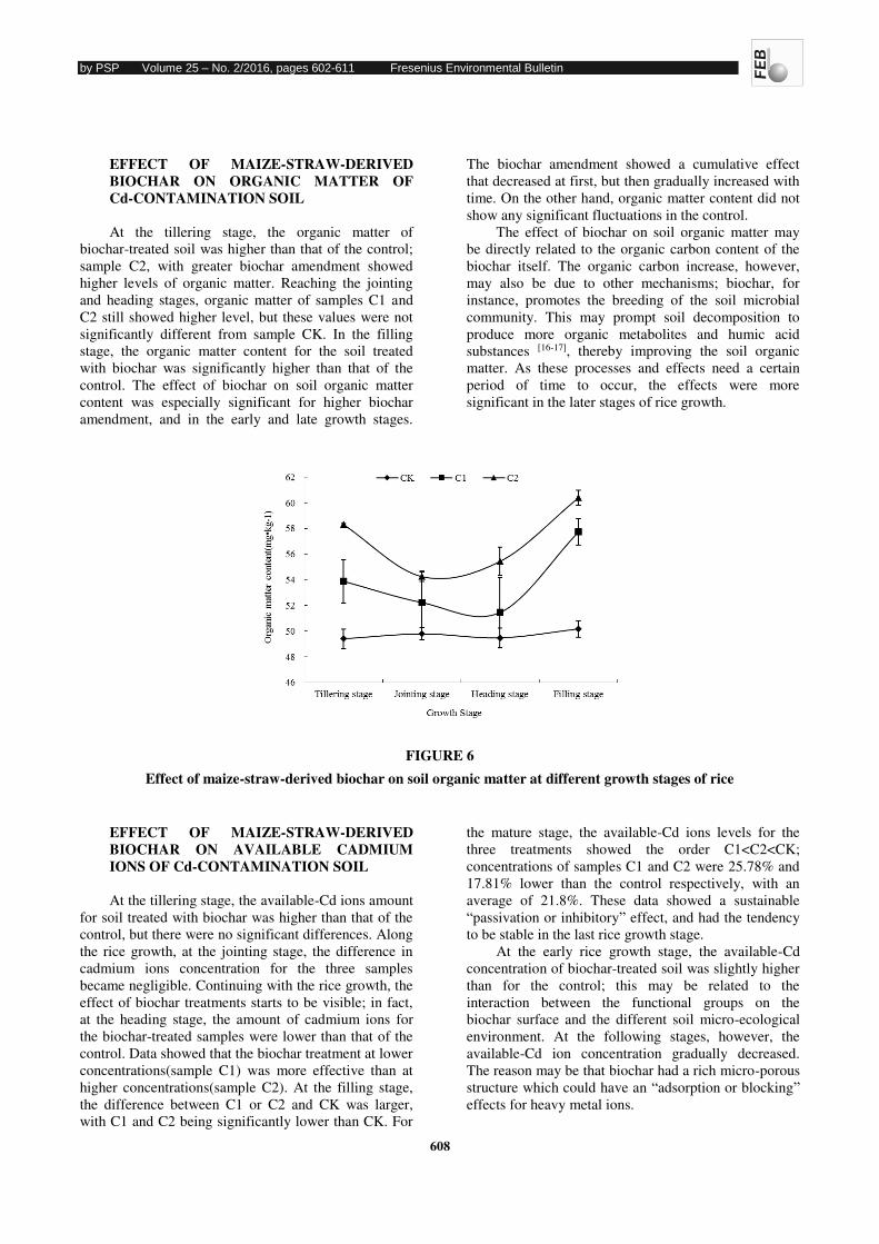
by PSP Volume 25 – No. 2/2016, pages 602-611 Fresenius Environmental Bulletin
608
EFFECT OF MAIZE-STRAW-DERIVED
BIOCHAR ON ORGANIC MATTER OF
Cd-CONTAMINATION SOIL
At the tillering stage, the organic matter of
biochar-treated soil was higher than that of the control;
sample C2, with greater biochar amendment showed
higher levels of organic matter. Reaching the jointing
and heading stages, organic matter of samples C1 and
C2 still showed higher level, but these values were not
significantly different from sample CK. In the filling
stage, the organic matter content for the soil treated
with biochar was significantly higher than that of the
control. The effect of biochar on soil organic matter
content was especially significant for higher biochar
amendment, and in the early and late growth stages.
The biochar amendment showed a cumulative effect
that decreased at first, but then gradually increased with
time. On the other hand, organic matter content did not
show any significant fluctuations in the control.
The effect of biochar on soil organic matter may
be directly related to the organic carbon content of the
biochar itself. The organic carbon increase, however,
may also be due to other mechanisms; biochar, for
instance, promotes the breeding of the soil microbial
community. This may prompt soil decomposition to
produce more organic metabolites and humic acid
substances [16-17], thereby improving the soil organic
matter. As these processes and effects need a certain
period of time to occur, the effects were more
significant in the later stages of rice growth.
FIGURE 6
Effect of maize-straw-derived biochar on soil organic matter at different growth stages of rice
EFFECT OF MAIZE-STRAW-DERIVED
BIOCHAR ON AVAILABLE CADMIUM
IONS OF Cd-CONTAMINATION SOIL
At the tillering stage, the available-Cd ions amount
for soil treated with biochar was higher than that of the
control, but there were no significant differences. Along
the rice growth, at the jointing stage, the difference in
cadmium ions concentration for the three samples
became negligible. Continuing with the rice growth, the
effect of biochar treatments starts to be visible; in fact,
at the heading stage, the amount of cadmium ions for
the biochar-treated samples were lower than that of the
control. Data showed that the biochar treatment at lower
concentrations(sample C1) was more effective than at
higher concentrations(sample C2). At the filling stage,
the difference between C1 or C2 and CK was larger,
with C1 and C2 being significantly lower than CK. For
the mature stage, the available-Cd ions levels for the
three treatments showed the order C1<C2<CK;
concentrations of samples C1 and C2 were 25.78% and
17.81% lower than the control respectively, with an
average of 21.8%. These data showed a sustainable
“passivation or inhibitory” effect, and had the tendency
to be stable in the last rice growth stage.
At the early rice growth stage, the available-Cd
concentration of biochar-treated soil was slightly higher
than for the control; this may be related to the
interaction between the functional groups on the
biochar surface and the different soil micro-ecological
environment. At the following stages, however, the
available-Cd ion concentration gradually decreased.
The reason may be that biochar had a rich micro-porous
structure which could have an “adsorption or blocking”
effects for heavy metal ions.
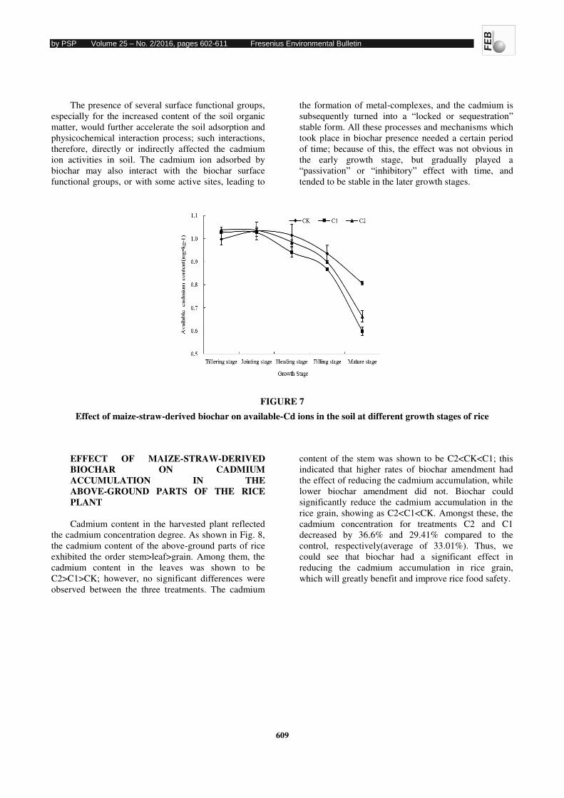
by PSP Volume 25 – No. 2/2016, pages 602-611 Fresenius Environmental Bulletin
609
The presence of several surface functional groups,
especially for the increased content of the soil organic
matter, would further accelerate the soil adsorption and
physicochemical interaction process; such interactions,
therefore, directly or indirectly affected the cadmium
ion activities in soil. The cadmium ion adsorbed by
biochar may also interact with the biochar surface
functional groups, or with some active sites, leading to
the formation of metal-complexes, and the cadmium is
subsequently turned into a “locked or sequestration”
stable form. All these processes and mechanisms which
took place in biochar presence needed a certain period
of time; because of this, the effect was not obvious in
the early growth stage, but gradually played a
“passivation” or “inhibitory” effect with time, and
tended to be stable in the later growth stages.
FIGURE 7
Effect of maize-straw-derived biochar on available-Cd ions in the soil at different growth stages of rice
EFFECT OF MAIZE-STRAW-DERIVED
BIOCHAR ON CADMIUM
ACCUMULATION IN THE
ABOVE-GROUND PARTS OF THE RICE
PLANT
Cadmium content in the harvested plant reflected
the cadmium concentration degree. As shown in Fig. 8,
the cadmium content of the above-ground parts of rice
exhibited the order stem>leaf>grain. Among them, the
cadmium content in the leaves was shown to be
C2>C1>CK; however, no significant differences were
observed between the three treatments. The cadmium
content of the stem was shown to be C2<CK<C1; this
indicated that higher rates of biochar amendment had
the effect of reducing the cadmium accumulation, while
lower biochar amendment did not. Biochar could
significantly reduce the cadmium accumulation in the
rice grain, showing as C2<C1<CK. Amongst these, the
cadmium concentration for treatments C2 and C1
decreased by 36.6% and 29.41% compared to the
control, respectively(average of 33.01%). Thus, we
could see that biochar had a significant effect in
reducing the cadmium accumulation in rice grain,
which will greatly benefit and improve rice food safety.
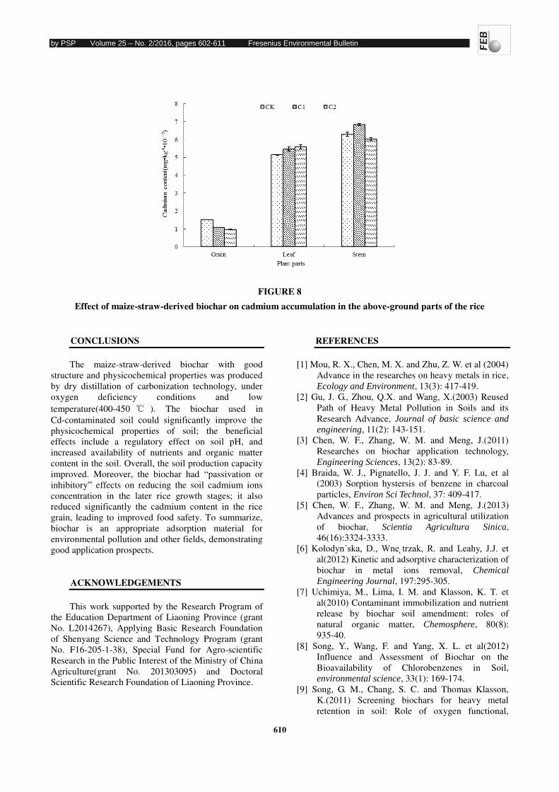
by PSP Volume 25 – No. 2/2016, pages 602-611 Fresenius Environmental Bulletin
610
FIGURE 8
Effect of maize-straw-derived biochar on cadmium accumulation in the above-ground parts of the rice
CONCLUSIONS
The maize-straw-derived biochar with good
structure and physicochemical properties was produced
by dry distillation of carbonization technology, under
oxygen deficiency conditions and low
temperature(400-450 ℃ ). The biochar used in
Cd-contaminated soil could significantly improve the
physicochemical properties of soil; the beneficial
effects include a regulatory effect on soil pH, and
increased availability of nutrients and organic matter
content in the soil. Overall, the soil production capacity
improved. Moreover, the biochar had “passivation or
inhibitory” effects on reducing the soil cadmium ions
concentration in the later rice growth stages; it also
reduced significantly the cadmium content in the rice
grain, leading to improved food safety. To summarize,
biochar is an appropriate adsorption material for
environmental pollution and other fields, demonstrating
good application prospects.
ACKNOWLEDGEMENTS
This work supported by the Research Program of
the Education Department of Liaoning Province (grant
No. L2014267), Applying Basic Research Foundation
of Shenyang Science and Technology Program (grant
No. F16-205-1-38), Special Fund for Agro-scientific
Research in the Public Interest of the Ministry of China
Agriculture(grant No. 201303095) and Doctoral
Scientific Research Foundation of Liaoning Province.
REFERENCES
[1] Mou, R. X., Chen, M. X. and Zhu, Z. W. et al (2004)
Advance in the researches on heavy metals in rice,
Ecology and Environment, 13(3): 417-419.
[2] Gu, J. G., Zhou, Q.X. and Wang, X.(2003) Reused
Path of Heavy Metal Pollution in Soils and its
Research Advance, Journal of basic science and
engineering, 11(2): 143-151.
[3] Chen, W. F., Zhang, W. M. and Meng, J.(2011)
Researches on biochar application technology,
Engineering Sciences, 13(2): 83-89.
[4] Braida, W. J., Pignatello, J. J. and Y. F. Lu, et al
(2003) Sorption hystersis of benzene in charcoal
particles, Environ Sci Technol, 37: 409-417.
[5] Chen, W. F., Zhang, W. M. and Meng, J.(2013)
Advances and prospects in agricultural utilization
of biochar, Scientia Agricultura Sinica,
46(16):3324-3333.
[6] Kołodyn´ska, D., Wne˛trzak, R. and Leahy, J.J. et al(2012) Kinetic and adsorptive characterization of
biochar in metal ions removal, Chemical
Engineering Journal, 197:295-305.
[7] Uchimiya, M., Lima, I. M. and Klasson, K. T. et
al(2010) Contaminant immobilization and nutrient
release by biochar soil amendment: roles of
natural organic matter, Chemosphere, 80(8):
935-40.
[8] Song, Y., Wang, F. and Yang, X. L. et al(2012)
Influence and Assessment of Biochar on the
Bioavailability of Chlorobenzenes in Soil,
environmental science, 33(1): 169-174.
[9] Song, G. M., Chang, S. C. and Thomas Klasson,
K.(2011) Screening biochars for heavy metal
retention in soil: Role of oxygen functional,
by PSP Volume 25 – No. 2/2016, pages 602-611 Fresenius Environmental Bulletin
611
Journal of hazardous materials, 190: 432-441.
[10] Sun, J. K., Lian, F. and Liu, Z. Q. et al(2014)
Biochars derived from various crops traws:
Characterization and Cd (II) Removal potential,
Ecotoxicology and Environmental Safety, 106:
226-231.
[11] Han, D., Liu, X. T. And Zhang, G.X. et al(2013)
Effects of cationic surfactant on prntachlorophenol
sorption by sediment, active carbon and biochar,
Fresenius Environmental Bulletin, 22: 1280-1286.
[12] Glaser, B., Lehmann, J. and Zech, W.(2002)
Ameliorating physical and chemical properties of
highly weathered soils in the tropics with
charcoal-a review, Biology Fertility of Soils, 35:
219-230.
[13] Lehmann, J., da Silva, J. P. and Steiner, C. et
al(2003) Nutrient availability and leaching in an
archaeological Anthrosol and a Ferralsol of the
Central Amazon basin: Fertilizer, manure and
charcoal amendments, Plant Soil, 249: 343-357.
[14] Laird, D. A., Fleming. P., and Davis, D. D., et
al(2010). Impact of biochar amendment on the
quality of a typical Midwestern agricultural soil.
Geoderma, 158: 443-449.
[15] Glaser, B., Lehmann, J. and Zech, W. (2002)
Ameliorating physical and chemical properties of
highly weathered soils in the tropics with
charcoal-a review, Biol Fert Soils, 35: 219-230.
[16] Saito, M. and Marumoto, T.(2002) Inoculation with
arbuscular mycorrhizal fungi: The status quo in
Japan and the future prospects, Plant Soil, 244:
273-279.
[17] Warnock, D. D., Lehmann, J. and Kuyper, T. W. et
al(2007) Mycorrhizal responses to biochar in
soil-concepts and mechanisms, Plant Soil, 300:
9-20.
Received: 20.08.2015
Accepted: 11.12.2015
CORRESPONDING AUTHOR
Wenfu Chen
Biochar Engineering Technology Research Center of
Liaoning Province
Agronomy College of Shenyang Agricultural
University
Shenyang – P.R. CHINA
e-mail: [email protected]
by PSP Volume 25 – No. 2/2016, pages 612-622 Fresenius Environmental Bulletin
612
TOXIC EFFECTS OF SILICA NANOPARTICLES ON HEART:
ELECTROPHYSIOLOGICAL, BIOCHEMICAL,
HISTOLOGICAL AND GENOTOXIC STUDY
Ebru Ballı1, Ülkü Çömelekoğlu2, Serap Yalın3, Dilek Battal4, Kasım Ocakoğlu5, Fatma Söğüt2, Selma
Yaman2, Çağatay Han Türkseven2, Pelin Eroğlu6, İlkay Karagül1, Gülşen Göney7, Saadet Yıldırımcan5,
Ayça Aktaş4
1Mersin University, Medical Faculty, Department of Histology and Embryology, Mersin, Turkey 2Mersin University, Medical Faculty, Department of Biophysics, Mersin, Turkey
3Mersin University, Pharmacy Faculty, Department of Biochemistry, Mersin, Turkey 4Mersin University, Pharmacy Faculty, Department of Pharmaceutical Toxicology, Mersin, Turkey
5 Mersin University Advanced Technology, Education, Research and Aplication Center, Mersin, Turkey 6Mersin University, Science and Letters Faculty, Department of Chemistry, Mersin, Turkey
7Gazi University, Pharmacy Faculty Department of Pharmaceutical Toxicology, Ankara, Turkey
ABSTRACT
In this study, the effect of variable sized silica
nanoparticles on the cardiac electrophysiology,
mechanics, antioxidant activity, ultrastructure and
genotoxicity in rats were investigated. Among five
groups (6, 20, 50 nm, control and positive control
for comet assay; n=7 for each group) treatment
groups received intraperitonally 150 µg/mL of
silica nanoparticles for 28 days. Electrical and
mechanical activities of heart were recorded using
electrophysiological recording techniques.
Malondialdehyde (MDA) levels, catalase (CAT)
and superoxide dismutase (SOD) activities were
measured using biochemical methodologies and
transmission electron microscopic levels of heart
samples were examined for all groups. Comet assay
was performed on peripheral blood lympocytes.
Heart rate significantly increased whereas
amplitude and duration of T wave decreased in 6
and 20 nm groups as compared with control group.
In 20 and 50 nm groups, P wave and QRS complex
amplitude were significantly higher and contraction
force were significantly lower than control.
Duration of contraction decreased and contraction
frequency increased in 6, 20 and 50 nm groups as
compared with control group. There was no
significant difference between control and silica
nanoparticle received groups for MDA levels, CAT
and SOD activities. Ultrastructurally, expansion in
endoplasmic reticulum cisterns, disorganization and
breaking off miyofibrils of myocytes were observed
in 6, 20 and 50 nm groups. In genotoxicity study,
tail length, tail intensity and tail moment of
peripheral blood lympocytes significantly decreased
in 20 and 50 nm groups as compared with positive
control group. According to our results, exposure to
different sizes SiNPs have a probable hazard
potential for the cardiac system.
KEYWORDS: silica nanoparticle, heart, ECG, contractility, antioxidant,
DNA damage
INTRODUCTION
Nanoparticles are defined as particles with a
diameter of less than 100 nm in structural
dimension. Because of the unique dimensional and
morphological properties, nanomaterials can be
physically and chemically manipulated and widely
used in industrial and biomedical processes [1-5].
This adds to the increasing industrial exposure to
SiNPs during production, transportation, storage,
and consumer use by which human exposure and
environmental burden were obviously increased.
Toxic effects of SiNPs were investigated by a
number of researchers in various tissues.
Hassankhani et al. [6] studied silicon dioxide
nanoparticles in healthy adult mice and showed that
SiNPs with diameters of 10-15 nm in size can cause
significant changes in albumin, cholesterol,
triglyceride, total protein, urea, HDL and LDL as
well as in alkaline phosphatase and aspartate
aminotransferase activity. Ahamed [7] investigated
SiNPs-induced cytotoxicity, oxidative stress and
apoptosis in cultured human skin epithelial (A431)
and human lung epithelial (A549) cells and he
showed that SiNPs induced cytotoxicity and
apoptosis in A431 and A549 cells. Zhang et al. [1]
studied toxic effects of ZnO, TiO2, SiO2 and Al2O3
nanoparticles on human fetal lung fibroblasts and
they suggested that the four types of metal oxide
nanoparticles lead to cellular mitochondrial
dysfunction, morphological modifications and
apoptosis. Ramesh et al. [8] designed to investigate
the oxidative toxic effects of silicon dioxide
nanoparticles using fish model. Their results
revealed that alteration of antioxidant enzymes due
by PSP Volume 25 – No. 2/2016, pages 612-622 Fresenius Environmental Bulletin
613
to SiNPs can be considered as a biomarker to SiO2-
mediated oxidative stress in biological samples.
Duan et al. [9] studied cardiovascular toxicity of
SiNPs in endothelial cells and zebrafish model.
They revealed that SiNPs could inhibit the
angiogenesis and disturb the heart formation and
development. They suggested that exposure to
SiNPs is a possible risk factor to cardiovascular
system. Despite these, Galagudza et al. [10]
suggested carbon and SiNPs are nontoxic materials
that can be used as carriers for heart targeted drug
delivery.
As shown, there are only a few publications
studying the effects of nanoparticles on
cardiovascular parameters. In this study, therefore,
we aimed to investigate the effect of variable sized
(6 nm, 20 nm and 50 nm) SiNPs on cardiac
contraction, ECG parameters, cardiac ultrastructure,
oxidative stress markers and genotoxicity.
MATERIAL AND METHODS
The SiNPs were prepared according to the
procedures reported in the literature [11,12]. X-ray
powder diffraction (XRD) measurements were
carried out using Bruker D8 Advance X-ray
diffractometer. Transmission electron microscopy
(TEM) was used to characterize particle size and
shape of the nanoparticles. TEM images were
obtained with a JEOL JEM-2100F using
formvar/carbon coated 200-mesh copper grids.
The preparation of SiNPs. SiNPs were
synthesized using the Stöber method according to
the previously reported procedures in the literature
[11,12]. In a typical synthesis, 1.2 mL TEOS, 0.1
mL APTES, 1.2 mL NH4OH and 5 mL ethanol
were mixed homogeneously under an inert
atmosphere (overnight). Then, the nanoparticles
were washed with absolute ethanol for five times to
remove unreacted chemicals. The sizes of
nanoparticles were adjusted by changing the
precursor concentrations. In addition to our
previously reported study, the nanoparticles were
characterized by XRD and TEM [11]. A Bruker D8
Advanced Series powder diffractometer at ambient
temperature (40 kV, 40 mA, Cu Kα λ=1.5405 Å) was used for XRD measurements. For medical
applications, the nanoparticles were dispersed in a
saline solution at a concentration of 150 µg/mL by
ultrasonication, and then were filtered by an
appropriate filter [11].
Animals. Thirty-five healthy adult male
Wistar albino rats weighing 150–250 g were used
in this study and maintained in stainless steel cages
under controlled temperature (22°C) and humidity
(55–60%) with a 12-hr light–dark cycle. Standard
laboratory rat feed containing 21% protein and
fresh drinking water was given ad libitum. The
animals were treated humanely with regard to
alleviation of suffering and the study protocol was
designed according to the ethical standards for
animal use and approved by the local Committee of
Animal Use at Mersin University.
Experimental Design. Thirty five male
Wistar albino rats were equally divided into five
groups (n=7 rats) which were treated with SiNPs in
physiological serum intraperitoneally (i.p) in a
volume of 1 mL. Group 1 was the control
(physiological serum treated) group. Group 2 was
administered low particule size SiNP (6 nm, 150
µg/mL/day). Group 3 was treated with medium
particule size SiNP (20 nm, 150 µg/mL/day). Group
4 received high particule size SiNP (50 nm, 150
µg/mL/day) once a day throughout 28 days of the
study for chronic treatment. Group 5 was positive
control group, ethylmethane sulfonate (EMS; CAS
No. 62-50-0) was dissolved in physiological serum
and administred i.p 200 mg/kg BW, 24 h before
sacrifice.
Electrocardiogram. Animals were
anesthetized using 50 mg/kg intramuscular
ketamine hydrochloride. The electrical activity of
heart was recorded using the BIOPAC MP 100
Acquisition System Version 3.5.7 (Santa Barbara,
USA). The signals were digitized with a 16-bit
analog-to-digital converter at a sampling rate of
2500 samples/s. BIOPAC Acknowledge Analysis
Software (ACK 100 W5.7 version) was used to
measure the heart rate, the amplitude and the
duration of the P wave, QRS complex and T wave.
Mechanogram. After electrocardiogram
records, an incision was made to leave the
midabdominal line, starting from the inferior
portion of the abdominal cavity. To reach the heart,
the left and right sides of the sternum were incised
(to avoid cardiac perforation). The heart was
separated carefully from the pericardial sac. Apical
force displacement was used to measure cardiac
contractility [13]. The signals were digitized with a
16-bit analog-to-digital converter at a sampling rate
of 500 samples/s. BIOPAC Acknowledge Analysis
Software was used to measure the ventricular force
and the ventricular contraction time and the
frequency of contraction from mechanogram.
Biochemical evaluation. Tissue samples were
homogenized (T25 Ultra-Turrax, IKA Werke
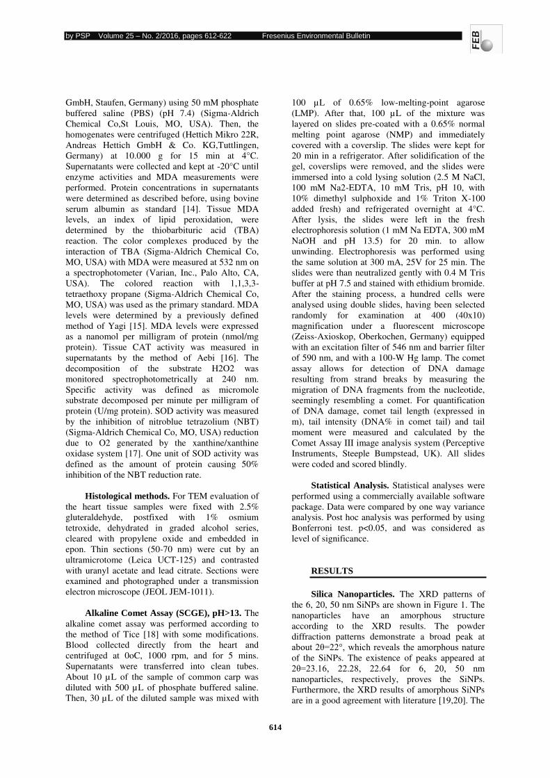
by PSP Volume 25 – No. 2/2016, pages 612-622 Fresenius Environmental Bulletin
614
GmbH, Staufen, Germany) using 50 mM phosphate
buffered saline (PBS) (pH 7.4) (Sigma-Aldrich
Chemical Co,St Louis, MO, USA). Then, the
homogenates were centrifuged (Hettich Mikro 22R,
Andreas Hettich GmbH & Co. KG,Tuttlingen,
Germany) at 10.000 g for 15 min at 4°C.
Supernatants were collected and kept at -20°C until
enzyme activities and MDA measurements were
performed. Protein concentrations in supernatants
were determined as described before, using bovine
serum albumin as standard [14]. Tissue MDA
levels, an index of lipid peroxidation, were
determined by the thiobarbituric acid (TBA)
reaction. The color complexes produced by the
interaction of TBA (Sigma-Aldrich Chemical Co,
MO, USA) with MDA were measured at 532 nm on
a spectrophotometer (Varian, Inc., Palo Alto, CA,
USA). The colored reaction with 1,1,3,3-
tetraethoxy propane (Sigma-Aldrich Chemical Co,
MO, USA) was used as the primary standard. MDA
levels were determined by a previously defined
method of Yagi [15]. MDA levels were expressed
as a nanomol per milligram of protein (nmol/mg
protein). Tissue CAT activity was measured in
supernatants by the method of Aebi [16]. The
decomposition of the substrate H2O2 was
monitored spectrophotometrically at 240 nm.
Specific activity was defined as micromole
substrate decomposed per minute per milligram of
protein (U/mg protein). SOD activity was measured
by the inhibition of nitroblue tetrazolium (NBT)
(Sigma-Aldrich Chemical Co, MO, USA) reduction
due to O2 generated by the xanthine/xanthine
oxidase system [17]. One unit of SOD activity was
defined as the amount of protein causing 50%
inhibition of the NBT reduction rate.
Histological methods. For TEM evaluation of
the heart tissue samples were fixed with 2.5%
gluteraldehyde, postfixed with 1% osmium
tetroxide, dehydrated in graded alcohol series,
cleared with propylene oxide and embedded in
epon. Thin sections (50-70 nm) were cut by an
ultramicrotome (Leica UCT-125) and contrasted
with uranyl acetate and lead citrate. Sections were
examined and photographed under a transmission
electron microscope (JEOL JEM-1011).
Alkaline Comet Assay (SCGE), pH>13. The
alkaline comet assay was performed according to
the method of Tice [18] with some modifications.
Blood collected directly from the heart and
centrifuged at 0oC, 1000 rpm, and for 5 mins.
Supernatants were transferred into clean tubes.
About 10 µL of the sample of common carp was
diluted with 500 µL of phosphate buffered saline.
Then, 30 µL of the diluted sample was mixed with
100 µL of 0.65% low-melting-point agarose
(LMP). After that, 100 µL of the mixture was
layered on slides pre-coated with a 0.65% normal
melting point agarose (NMP) and immediately
covered with a coverslip. The slides were kept for
20 min in a refrigerator. After solidification of the
gel, coverslips were removed, and the slides were
immersed into a cold lysing solution (2.5 M NaCl,
100 mM Na2-EDTA, 10 mM Tris, pH 10, with
10% dimethyl sulphoxide and 1% Triton X-100
added fresh) and refrigerated overnight at 4°C.
After lysis, the slides were left in the fresh
electrophoresis solution (1 mM Na EDTA, 300 mM
NaOH and pH 13.5) for 20 min. to allow
unwinding. Electrophoresis was performed using
the same solution at 300 mA, 25V for 25 min. The
slides were than neutralized gently with 0.4 M Tris
buffer at pH 7.5 and stained with ethidium bromide.
After the staining process, a hundred cells were
analysed using double slides, having been selected
randomly for examination at 400 (40x10)
magnification under a fluorescent microscope
(Zeiss-Axioskop, Oberkochen, Germany) equipped
with an excitation filter of 546 nm and barrier filter
of 590 nm, and with a 100-W Hg lamp. The comet
assay allows for detection of DNA damage
resulting from strand breaks by measuring the
migration of DNA fragments from the nucleotide,
seemingly resembling a comet. For quantification
of DNA damage, comet tail length (expressed in
m), tail intensity (DNA% in comet tail) and tail
moment were measured and calculated by the
Comet Assay III image analysis system (Perceptive
Instruments, Steeple Bumpstead, UK). All slides
were coded and scored blindly.
Statistical Analysis. Statistical analyses were
performed using a commercially available software
package. Data were compared by one way variance
analysis. Post hoc analysis was performed by using
Bonferroni test. p<0.05, and was considered as
level of significance.
RESULTS
Silica Nanoparticles. The XRD patterns of
the 6, 20, 50 nm SiNPs are shown in Figure 1. The
nanoparticles have an amorphous structure
according to the XRD results. The powder
diffraction patterns demonstrate a broad peak at
about 2θ=22°, which reveals the amorphous nature of the SiNPs. The existence of peaks appeared at
2θ=23.16, 22.28, 22.64 for 6, 20, 50 nm nanoparticles, respectively, proves the SiNPs.
Furthermore, the XRD results of amorphous SiNPs
are in a good agreement with literature [19,20]. The
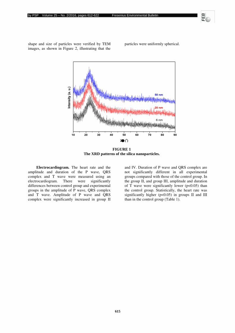
by PSP Volume 25 – No. 2/2016, pages 612-622 Fresenius Environmental Bulletin
615
shape and size of particles were verified by TEM
images, as shown in Figure 2, illustrating that the
particles were uniformly spherical.
10 20 30 40 50 60 70 80 90
Inte
ns
ity
(a
. u
.)
2(o)
6 nm
20 nm
50 nm
FIGURE 1
The XRD patterns of the silica nanoparticles.
Electrocardiogram. The heart rate and the
amplitude and duration of the P wave, QRS
complex and T wave were measured using an
electrocardiogram. There were significantly
differences between control group and experimental
groups in the amplitude of P wave, QRS complex
and T wave. Amplitude of P wave and QRS
complex were significantly increased in group II
and IV. Duration of P wave and QRS complex are
not significantly different in all experimental
groups compared with those of the control group. In
the group II, and group III, amplitude and duration
of T wave were significantly lower (p<0.05) than
the control group. Statistically, the heart rate was
significantly higher (p<0.05) in groups II and III
than in the control group (Table 1).
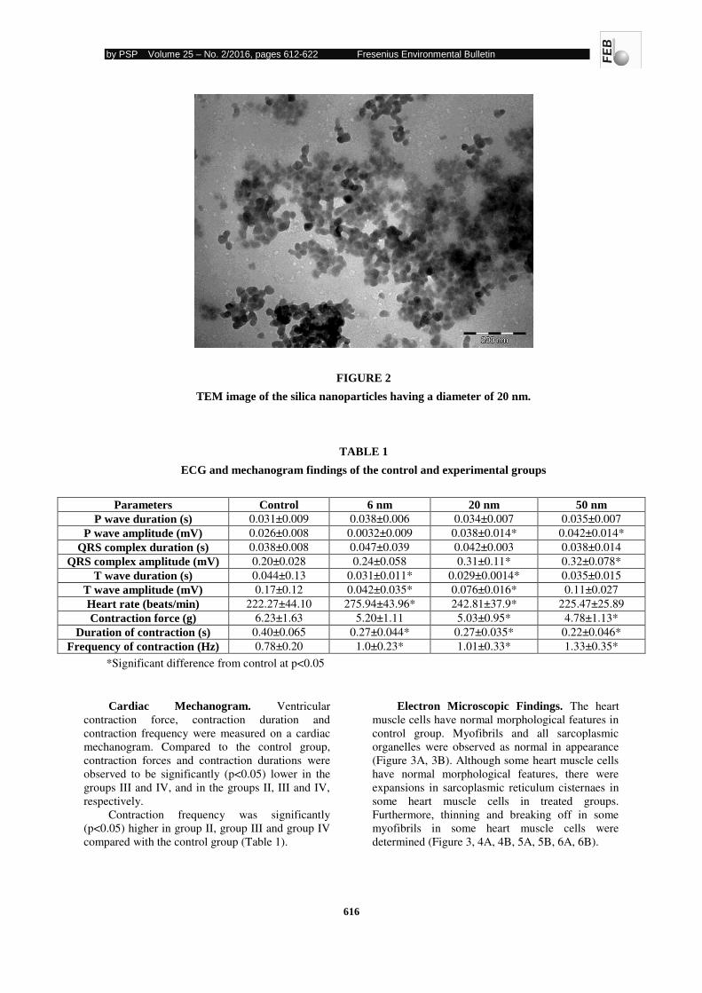
by PSP Volume 25 – No. 2/2016, pages 612-622 Fresenius Environmental Bulletin
616
FIGURE 2
TEM image of the silica nanoparticles having a diameter of 20 nm.
TABLE 1
ECG and mechanogram findings of the control and experimental groups
Parameters Control 6 nm 20 nm 50 nm
P wave duration (s) 0.031±0.009 0.038±0.006 0.034±0.007 0.035±0.007
P wave amplitude (mV) 0.026±0.008 0.0032±0.009 0.038±0.014* 0.042±0.014*
QRS complex duration (s) 0.038±0.008 0.047±0.039 0.042±0.003 0.038±0.014
QRS complex amplitude (mV) 0.20±0.028 0.24±0.058 0.31±0.11* 0.32±0.078*
T wave duration (s) 0.044±0.13 0.031±0.011* 0.029±0.0014* 0.035±0.015
T wave amplitude (mV) 0.17±0.12 0.042±0.035* 0.076±0.016* 0.11±0.027
Heart rate (beats/min) 222.27±44.10 275.94±43.96* 242.81±37.9* 225.47±25.89
Contraction force (g) 6.23±1.63 5.20±1.11 5.03±0.95* 4.78±1.13*
Duration of contraction (s) 0.40±0.065 0.27±0.044* 0.27±0.035* 0.22±0.046*
Frequency of contraction (Hz) 0.78±0.20 1.0±0.23* 1.01±0.33* 1.33±0.35*
*Significant difference from control at p<0.05
Cardiac Mechanogram. Ventricular
contraction force, contraction duration and
contraction frequency were measured on a cardiac
mechanogram. Compared to the control group,
contraction forces and contraction durations were
observed to be significantly (p<0.05) lower in the
groups III and IV, and in the groups II, III and IV,
respectively.
Contraction frequency was significantly
(p<0.05) higher in group II, group III and group IV
compared with the control group (Table 1).
Electron Microscopic Findings. The heart
muscle cells have normal morphological features in
control group. Myofibrils and all sarcoplasmic
organelles were observed as normal in appearance
(Figure 3A, 3B). Although some heart muscle cells
have normal morphological features, there were
expansions in sarcoplasmic reticulum cisternaes in
some heart muscle cells in treated groups.
Furthermore, thinning and breaking off in some
myofibrils in some heart muscle cells were
determined (Figure 3, 4A, 4B, 5A, 5B, 6A, 6B).
by PSP Volume 25 – No. 2/2016, pages 612-622 Fresenius Environmental Bulletin
617
FIGURE 3
Control group. The heart muscle cells have normal morphologic characteristics. Mitochondrion
(arrow head), discus intercalaris (thick arrow), sarcoplasmic reticulum cisternaes (thin arrow) - x10.000.
TABLE 2
Antioxidant enzyme activities and MDA levels
Control 6 nm 20 nm 50 nm
CAT (U/mg protein) 141.58±24.36 113.98±50.05 92.23±40.62 189.16±76.45
SOD (U/mg protein) 2.42±1.30 2.24±0.73 1.45±0.41 1.54±0.81
MDA (nmol/mg
protein) 6.10±3.03 10.29±5.93 8.36±4.05 7.21±3.01
Antioxidant enzyme activities and MDA
levels. The generation of intracellular reactive
oxygen species (ROS) could cause oxidative
damage. Therefore, we measured the production of
MDA as well as the activities of SOD and CAT. As
shown Table 2, administration of SiNPs caused no
significant change in SOD, CAT activities and
MDA levels in all experimental groups compared to
control group (p>0.05).
Blood Comet Assay. Comet assay data
presented as median and (25-75%) based on 100
cells scored per animal. In comparison with the
positive control group, tail length, tail intensity and
tail moment of blood cells exposed to 20 nm and 50
nm SiNPs significantly decreased (Table 3). There
was a statistically significant difference according
to percentage of tail intensity of blood lymphocyte
cell results between 6, 20 and 50 nm nanoparticules
and positive control (Table 3).
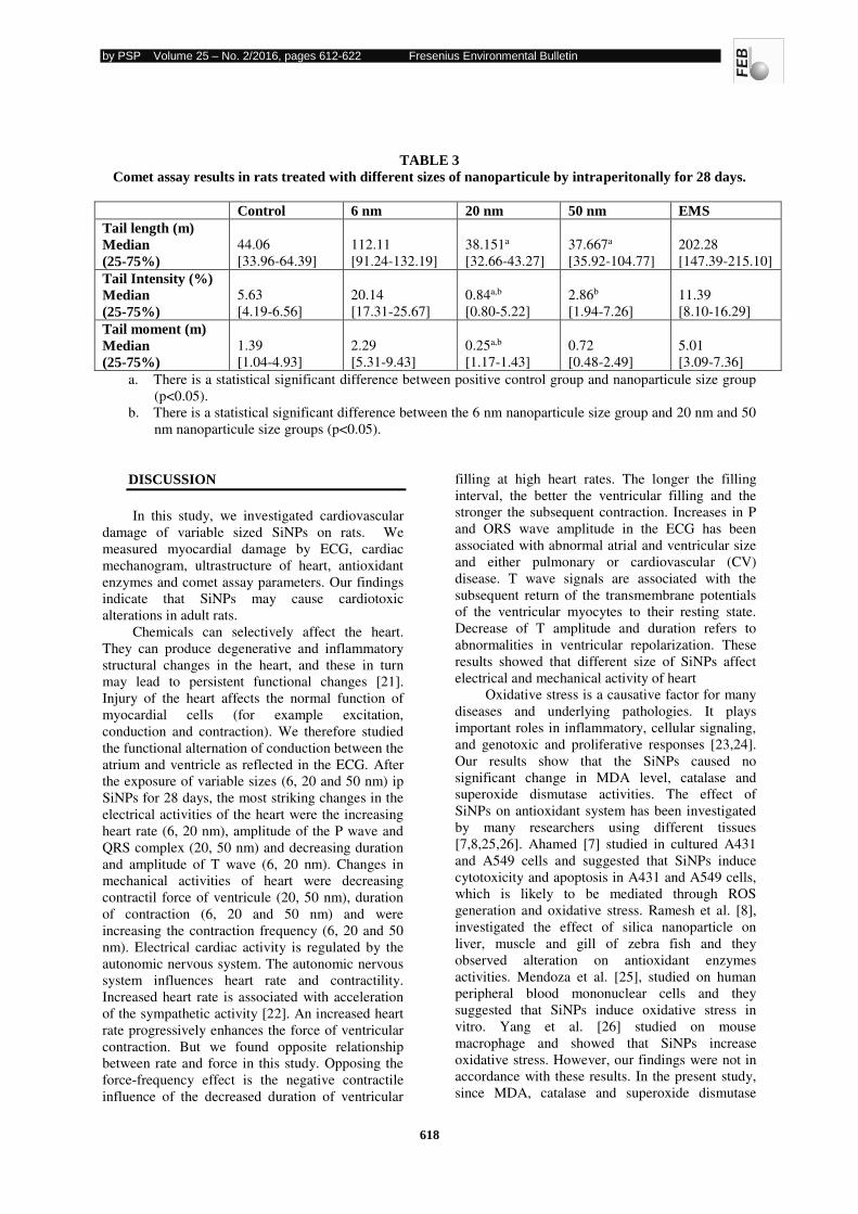
by PSP Volume 25 – No. 2/2016, pages 612-622 Fresenius Environmental Bulletin
618
TABLE 3
Comet assay results in rats treated with different sizes of nanoparticule by intraperitonally for 28 days.
Control 6 nm 20 nm 50 nm EMS
Tail length (m)
Median
(25-75%)
44.06
[33.96-64.39]
112.11
[91.24-132.19]
38.151a
[32.66-43.27]
37.667a
[35.92-104.77]
202.28
[147.39-215.10]
Tail Intensity (%)
Median
(25-75%)
5.63
[4.19-6.56]
20.14
[17.31-25.67]
0.84a,b
[0.80-5.22]
2.86b
[1.94-7.26]
11.39
[8.10-16.29]
Tail moment (m)
Median
(25-75%)
1.39
[1.04-4.93]
2.29
[5.31-9.43]
0.25a,b
[1.17-1.43]
0.72
[0.48-2.49]
5.01
[3.09-7.36]
a. There is a statistical significant difference between positive control group and nanoparticule size group
(p<0.05).
b. There is a statistical significant difference between the 6 nm nanoparticule size group and 20 nm and 50
nm nanoparticule size groups (p<0.05).
DISCUSSION
In this study, we investigated cardiovascular
damage of variable sized SiNPs on rats. We
measured myocardial damage by ECG, cardiac
mechanogram, ultrastructure of heart, antioxidant
enzymes and comet assay parameters. Our findings
indicate that SiNPs may cause cardiotoxic
alterations in adult rats.
Chemicals can selectively affect the heart.
They can produce degenerative and inflammatory
structural changes in the heart, and these in turn
may lead to persistent functional changes [21].
Injury of the heart affects the normal function of
myocardial cells (for example excitation,
conduction and contraction). We therefore studied
the functional alternation of conduction between the
atrium and ventricle as reflected in the ECG. After
the exposure of variable sizes (6, 20 and 50 nm) ip
SiNPs for 28 days, the most striking changes in the
electrical activities of the heart were the increasing
heart rate (6, 20 nm), amplitude of the P wave and
QRS complex (20, 50 nm) and decreasing duration
and amplitude of T wave (6, 20 nm). Changes in
mechanical activities of heart were decreasing
contractil force of ventricule (20, 50 nm), duration
of contraction (6, 20 and 50 nm) and were
increasing the contraction frequency (6, 20 and 50
nm). Electrical cardiac activity is regulated by the
autonomic nervous system. The autonomic nervous
system influences heart rate and contractility.
Increased heart rate is associated with acceleration
of the sympathetic activity [22]. An increased heart
rate progressively enhances the force of ventricular
contraction. But we found opposite relationship
between rate and force in this study. Opposing the
force-frequency effect is the negative contractile
influence of the decreased duration of ventricular
filling at high heart rates. The longer the filling
interval, the better the ventricular filling and the
stronger the subsequent contraction. Increases in P
and ORS wave amplitude in the ECG has been
associated with abnormal atrial and ventricular size
and either pulmonary or cardiovascular (CV)
disease. T wave signals are associated with the
subsequent return of the transmembrane potentials
of the ventricular myocytes to their resting state.
Decrease of T amplitude and duration refers to
abnormalities in ventricular repolarization. These
results showed that different size of SiNPs affect
electrical and mechanical activity of heart
Oxidative stress is a causative factor for many
diseases and underlying pathologies. It plays
important roles in inflammatory, cellular signaling,
and genotoxic and proliferative responses [23,24].
Our results show that the SiNPs caused no
significant change in MDA level, catalase and
superoxide dismutase activities. The effect of
SiNPs on antioxidant system has been investigated
by many researchers using different tissues
[7,8,25,26]. Ahamed [7] studied in cultured A431
and A549 cells and suggested that SiNPs induce
cytotoxicity and apoptosis in A431 and A549 cells,
which is likely to be mediated through ROS
generation and oxidative stress. Ramesh et al. [8],
investigated the effect of silica nanoparticle on
liver, muscle and gill of zebra fish and they
observed alteration on antioxidant enzymes
activities. Mendoza et al. [25], studied on human
peripheral blood mononuclear cells and they
suggested that SiNPs induce oxidative stress in
vitro. Yang et al. [26] studied on mouse
macrophage and showed that SiNPs increase
oxidative stress. However, our findings were not in
accordance with these results. In the present study,
since MDA, catalase and superoxide dismutase
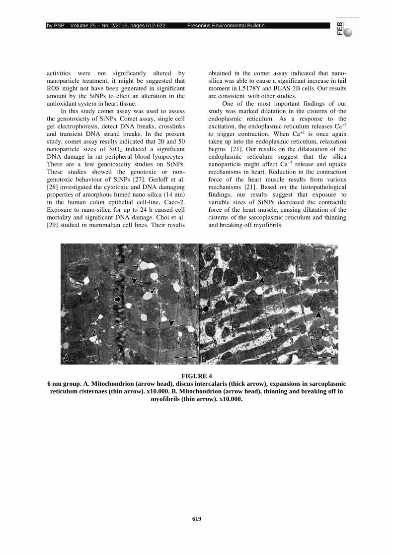
by PSP Volume 25 – No. 2/2016, pages 612-622 Fresenius Environmental Bulletin
619
activities were not significantly altered by
nanoparticle treatment, it might be suggested that
ROS might not have been generated in significant
amount by the SiNPs to elicit an alteration in the
antioxidant system in heart tissue.
In this study comet assay was used to assess
the genotoxicity of SiNPs. Comet assay, single cell
gel electrophoresis, detect DNA breaks, crosslinks
and transient DNA strand breaks. In the present
study, comet assay results indicated that 20 and 50
nanoparticle sizes of SiO2 induced a significant
DNA damage in rat peripheral blood lympocytes.
There are a few genotoxicity studies on SiNPs.
These studies showed the genotoxic or non-
genotoxic behaviour of SiNPs [27]. Gerloff et al.
[28] investigated the cytotoxic and DNA damaging
properties of amorphous fumed nano-silica (14 nm)
in the human colon epithelial cell-line, Caco-2.
Exposure to nano-silica for up to 24 h caused cell
mortality and significant DNA damage. Choi et al.
[29] studied in mammalian cell lines. Their results
obtained in the comet assay indicated that nano-
silica was able to cause a significant increase in tail
moment in L5178Y and BEAS-2B cells. Our results
are consistent with other studies.
One of the most important findings of our
study was marked dilatation in the cisterns of the
endoplasmic reticulum. As a response to the
excitation, the endoplasmic reticulum releases Ca+2
to trigger contraction. When Ca+2 is once again
taken up into the endoplasmic reticulum, relaxation
begins [21]. Our results on the dilatatation of the
endoplasmic reticulum suggest that the silica
nanoparticle might affect Ca+2 release and uptake
mechanisms in heart. Reduction in the contraction
force of the heart muscle results from various
mechanisms [21]. Based on the histopathological
findings, our results suggest that exposure to
variable sizes of SiNPs decreased the contractile
force of the heart muscle, causing dilatation of the
cisterns of the sarcoplasmic reticulum and thinning
and breaking off myofibrils.
FIGURE 4
6 nm group. A. Mitochondrion (arrow head), discus intercalaris (thick arrow), expansions in sarcoplasmic
reticulum cisternaes (thin arrow). x10.000. B. Mitochondrion (arrow head), thinning and breaking off in
myofibrils (thin arrow). x10.000.
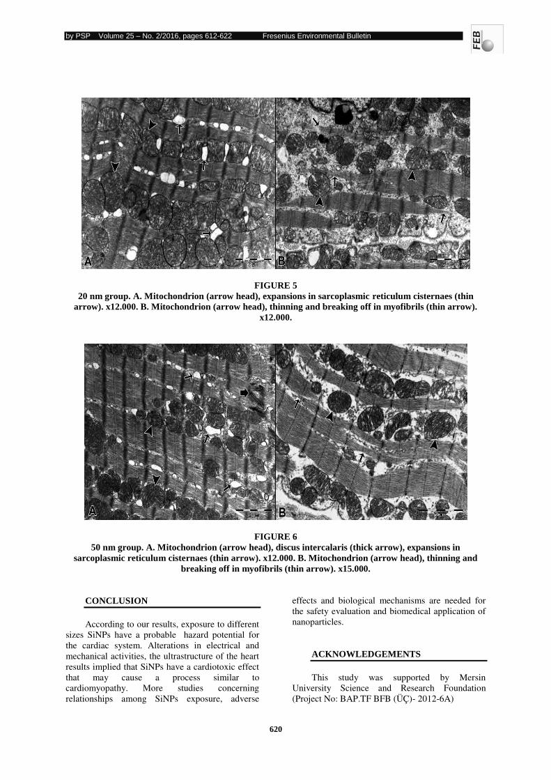
by PSP Volume 25 – No. 2/2016, pages 612-622 Fresenius Environmental Bulletin
620
FIGURE 5
20 nm group. A. Mitochondrion (arrow head), expansions in sarcoplasmic reticulum cisternaes (thin
arrow). x12.000. B. Mitochondrion (arrow head), thinning and breaking off in myofibrils (thin arrow).
x12.000.
FIGURE 6
50 nm group. A. Mitochondrion (arrow head), discus intercalaris (thick arrow), expansions in
sarcoplasmic reticulum cisternaes (thin arrow). x12.000. B. Mitochondrion (arrow head), thinning and
breaking off in myofibrils (thin arrow). x15.000.
CONCLUSION
According to our results, exposure to different
sizes SiNPs have a probable hazard potential for
the cardiac system. Alterations in electrical and
mechanical activities, the ultrastructure of the heart
results implied that SiNPs have a cardiotoxic effect
that may cause a process similar to
cardiomyopathy. More studies concerning
relationships among SiNPs exposure, adverse
effects and biological mechanisms are needed for
the safety evaluation and biomedical application of
nanoparticles.
ACKNOWLEDGEMENTS
This study was supported by Mersin
University Science and Research Foundation
(Project No: BAP.TF BFB (ÜÇ)- 2012-6A)
by PSP Volume 25 – No. 2/2016, pages 612-622 Fresenius Environmental Bulletin
621
CONFLICTS OF INTEREST
The authors report no conflicts of interest.
REFERENCES
[1] Zhang, X.Q., Yin, L.H., Tang, M., Pu, Y.P.
(2011) ZnO, TiO2, SiO2, and Al2O3
nanoparticles-induced toxic effects on human
fetal lung fibroblasts. Biomed Environ Sci
24:661-669.
[2] Kumar, R., Roy, I., Ohulchanskky, T.Y. et al.
(2010) In vivo biodistribution and clearance
studies using multimodal organically modified
silica nanoparticles. ACS Nano 23:699-708.
[3] Li, Z., Barnes, J.C., Bosoy, A., Stoddart, J.F.,
Zink, J.I. (2012) Mesoporous silica
nanoparticles in biomedical applications.
Chem Soc Rev 41:2590-2605.
[4] Barandeh, F., Nguyen, P.L., Kumar, R., et al.
(2012) Organically modified silica
nanoparticles are biocompatible and can be
targeted to neurons in vivo. PLoS One 7:
e29424.
[5] Lee, J.E., Lee, N., Kim, T., Kim, J., Hyeon, T.
(2011) Multifunctional mesoporous silica
nanocomposite nanoparticles for theranostic
applications. Acc Chem Res 44893-44902.
[6] Hassankhani, R., Esmaeillou, M., Tehrani, A.A.,
Nasirzadeh, K., Khadir, F., Maadi, H. (2014)
In vivo toxicity of orally administrated silicon
dioxide nanoparticles in healthy adult mice.
Environ. Sci Pollut Res Int 22:1127-1132.
[7] Ahamed, M. (2013) Silica nanoparticles-
induced cytotoxicity, oxidative stress and
apoptosis in cultured A431 and A549 cells.
Hum Exp Toxicol 32:186-195.
[8] Ramesh, R., Kavitha, P., Kanipandian, N.,
Arun, S., Thirumurugan, R., Subramanian, P.
(2013) Alteration of antioxidant enzymes and
impairment of DNA in the silica nanoparticles
exposed zebra fish (Danio rerio). Environ
Monit Assess 185:5873-5881.
[9] Duan, J., Yu, Y., Li, Y., et al. (2013) Toxic
effect of silica nanoparticles on endothelial
cells through DNA damage response via
Chk1-dependent G2/M checkpoint. PLoS One
8:e62087.
[10] Galagudza, M.M., Korolev, D.V., Sonin, D.L.,
et al. (2010) Targeted drug delivery into
reversibly injured myocardium with silica
nanoparticles: surface functionalization,
natural biodistribution, and acute toxicity. Int J
Nanomedicine 5:231-237.
[11] Battal, D., Celik, A., Güler, G., et al. (2014)
SiO2 nanoparticule-induced size-dependent
genotoxicity – an in vitro study using sister
chromatid exchange, micronucleus and comet
assay. Drug Chem Toxicol 1-9. [Epub ahead
of print]
[12] Costa, C.A.R., Valadares, L.F., Galembeck, F.
(2007) Stöber silica particle size effect on the
hardness and brittleness of silica monoliths.
Colloids Surfaces A: Physicochem Eng
Aspects 302:371-376.
[13] Kleinelp, W.C. (1991) Experiments in
Physiology. North Brunswick: Wood River
Publications,
[14] Lowry, O.H., Rosenbrough, N.J., Farr, A.L.,
Randall, R.J. (1951) Protein measurement
with the Folin phenol reagent. J Biol Chem
193:265-275.
[15] Yagi, K. (1998) Simple procedure for specific
enzyme of lipid hydroperoxides in serum or
plasma. Methods Mol Biol 108:107-110.
[16] Aebi, H. (1984) Catalase in vitro. Methods
Enzymol 105:121-126.
[17] Sun, Y., Oberley, L.W., Li, Y. (1988) A simple
method for clinical assay of superoxide
dismutase. Clin Chem 34:497-500.
[18] Tice, R.R., Agurell, E., Anderson, D., et al,
(2000) Single cell gel/comet assay: guidelines
for in vitro and in vivo genetic toxicology
testing. Environ Mol Mutagen 35:206-221.
[19] Xuejing, C., Jianguo, J., Feng, Y., Sicong ,T.,
Kaimin, L. (2014) A novel low temperature
vapor phase hydrolysis method for the
production of nano-structured silica materials
using silicon tetrachloride. RSC Adv 4:8703-
8710.
[20] Banalata, S.K., Sanjana, P.D., Sumanta, K.S. et
al. (2013) Facile preparation of
multifunctional hollow silica nanoparticles
and their cancer specific targeting effect.
Biomater Sci 1:647-657.
[21] Hanig, J.P., Herman, E.H. (1991) Toxic
responses of the heart and vascular system. In:
Amdur MO, Daull J, Klaassen CD (eds)
Caserett and Daull's Toxicology: The Basic
Science of Poisons. Toronto: McGraw-Hill,
Pergamon, pp.430-461.
[22] Guyton, A.C., Hall, J.E. (1996) Textbook of
Medical Physiology. Philadelphia: W.B.
Saunders Company.
[23] Siddiqi, N.J., Abdelhalim, M.A.K., AlYafee,
Y.A., Alhomida, A.S. (2012) Studies on the
effect of gold nanoparticles on oxidative stress
and antioxidants defense indices in various rat
tissues. Afr J Pharm Pharmaco 6:3246-3251.
[24] Grigorov, B. (2012) Reactive oxygen species
and their relation to carcinogenesis. Trakia J
Sci 10:83-92.
by PSP Volume 25 – No. 2/2016, pages 612-622 Fresenius Environmental Bulletin
622
[25] Mendoza, A., Torres-Hernandez, J.A., Ault,
J.G., Pedersen-Lane, J.H., Gao, D., Lawrence,
D.A. (2014) Silica nanoparticles induce
oxidative stres and inflammation of human
peripheral blood mononuclear cells. Cell
Stress Chaperon 19:777-790.
[26] Yang, H., Wu, Q., Tang, M., Kong, L., Lu, Z.
(2009) Cell membrane injury induced by silica
nanoparticles in mouse macrophage. J
Biomed Nanotechnol 5(5):528-535.
[27] Golbamaki, N., Rasulev, B., Cassano, A., et al.
(2015) Genotoxicity of metal oxide
nanomaterials: review of recent data and
discussion of possible mechanisms. Nanoscale
7:2154-2198.
[28] Gerloff, K., Albrecht, C., Boots, A.W., Förster,
I., Schins, R.P.F. (2009) Cytotoxicity and
oxidative DNA damage by nanoparticles in
human intestinal Caco-2 cells.
Nanotoxicology 3:355-364.
[29] Choi, H.S., Kim, Y.J., Song, M., Song, M.K.,
Ryu, J.C. (2011) Genotoxicity of nano-silica
in mammalian cell lines. Toxicol Environ
Health Sci 3:7-13.
Received: 14.08.2015
Accepted: 18.12.2015
CORRESPONDING AUTHOR
Dr. Ulku Comelekoglu
Mersin University Medical School,
Department of Biophysics,
Mersin, 33169 – TURKEY
e-mail: [email protected]
by PSP Volume 25 – No. 2/2016, pages 623-632 Fresenius Environmental Bulletin
623
INFLUENCE OF LEAD STRESS ON GROWTH,
ANTIOXIDATIVE ENZYME ACTIVITIES AND ION CHANGE IN
ROOT AND LEAF OF STRAWBERRY
Ferhad Muradoğlu1, Tarık Encu2, Muttalip Gündoğdu1, Sibel Boysan Canal3
1Department of Horticulture, Faculty of Agriculture and Natural Sciences, Abant Izzet Baysal University, Bolu, Turkey.
2Department of Horticulture, Faculty of Agriculture, YuzuncuYil University, Van, Turkey 3Department of Soil science and Plant Nutrition, Faculty of Agriculture, YuzuncuYil University, Van, Turkey
ABSTRACT
Heavy metals are of widespread occurrence as
consequences of human, agricultural and industrial
activities. Among heavy metals, lead is a potential
pollutant that can accumulate in different tissues
organs and thus restrict plant growth. In this study,
mechanisms of plant tolerances to lead stress were
studied on strawberry (Camarosa cv.) using pot
experiment with different Lead Pb(NO3)2
applications ranging from 0 to 80 mg kg-1 using
soil culture. The accumulation of Pb2+ and its
influence on chlorophyll and malondialdehyde
(MDA) contents, activities of superoxide dismutase
(SOD), catalase (CAT), ascorbate peroxidase
(APX) and ion concentrations were investigated in
both root and leaves of strawberry plant. Despite
severally decrease in the chlorophyll a and b
contents, Pb2+ accumulation, MDA, SOD, and
CAT activities were increased with the increase in
the Pb2+concentrations both in roots and leaves.
However APX activity was shown unsteady
increase in roots and leaves. In the roots and leaves
macro and micro ion concentrations were shown
altered. While micro element concentrations
decreased in contrary to macro element
concentrations which were increased compare with
control. These results indicate that lead stress cause
reduction on growth and oxidative damage as
shown by the decline in chlorophyll, increase in
lipid peroxidase and antioxidant enzyme and alter
levels of macro-micro ion concentrations.
KEYWORDS:
Lead stress, antioxidant enzyme activity, lipid
peroxidase, macro-micro element, strawberry
INTRODUCTION
Lead is a toxic and residual environmental
pollution. The major source of Pb in environmental
are automobiles exhaust fumes , chimneys of
factories, wastes of the storage battery, processing
of Pb ores, metal plating and finishing activities,
pesticides, fertilizers, pigments additives and
gasoline [1]. Pb is accessible to plants from soil and
aerosol source. Pb can be accumulated into plants
though it is not necessary for plant. Previous studies
show that roots usually accumulate significant
quantities of Pb and roots greatly restricting its
translocation to aerial parts but certain species have
ability to transferring large quantities of Pb to their
shoot and leaves [2]. Many research demonstrated
that excess Pb causes toxic effect which influence
various morphological and biochemical processes
in plant. Pb toxicity inhibits cell division and
transpiration [3], chlorophyll production [4], leaf
rolls, chlorosis and inhibition of root and stem
growth [5], Lead to changes in plant nutrient upset
[6,7], changes hormonal status [1], water balance,
and nitrate assimilation [8]. Heavy metals cause
oxidative damage to plant either directly or
indirectly. ROS (reactive oxygen species) can
efficiently eliminated by non-enzymatic
components such as glutathione, ascorbic acid, a-
tocopherol and carotenoids as well as enzymatic
components superoxide dismutase (SOD),
ascorbate peroxidase (APX), catalase (CAT),
peroxidase (POD) and glutathione reductase,
ascorbic acid peroxidase [9, 10, 11]. Pb can cause
oxidative stress in plant with accompanying
increased ROS production. When exceeds the
capacity of cell defense mechanisms, these ROS
can induce oxidative stress and damage the
proteins, lipids and eventually causing the death of
plant [12, 13]. Turkey is one of the most important
countries in world with 353.173 tones Strawberry
productions. Turkey comes after United States of
America (1366.850) and Mexico (360.426) [14].
The strawberry is a grown area of around 134.23
decares in Turkey [15]. So ıt is very important to
study on Strawberry and understand the effect of Pb
toxicity in root and leaf of strawberry.
Up to the present, there is not study in the
literature dealing with Pb tolerance on strawberry
cultivars. Although, Pb toxicity in plant is depend
on Pb range, soil types and plant species. Thus, the
by PSP Volume 25 – No. 2/2016, pages 623-632 Fresenius Environmental Bulletin
624
objectives of the this study were study Pb
accumulation and influence of Pb toxicity on
Photosynthetic performance, ion alter in root and
leaf and also help to clarify Pb effect on antioxidant
enzymes in tolerances mechanisms in root and leaf
of Camarosa cultivars (Strawberry) in increasing Pb
applications.
MATERIAL AND METHODS
Plant materials and pot experiment. The
experiment was carried out in the green house of
YüzüncüYıl University during growing period (from middle May to end of July). The experiment
was conducted frigo plant of Strawberry (Fragaria x
ananassa cv. Camarosa) and pot experiment. Four
frigo plant was planted into every pots
(72x20x17cm) that were filled peat (4 kg). Initial
stage of grown, plants were fed by adding nutrient
solution to the pots. The nutrition solutions
contained N 200, K 208, P 37, Ca 167, Mg 49, Fe
1.53, Mn 1.16, B 0.46 Zn 0.09, Cu 0.03 and Mo
0.02 mg/L [16]. Flower buds were cut of early stage
of plant’s growth. After the plants had four or five leaves about 4 weeks, Lead applications were
started. Lead was added to pots at concentration of
0, 20, 60 and 80 mg kg-1 in the form of Pb(NO3)2
four equal times with watering during growth
period. In harvest, 12 plants were harvested to
every application, plants were sectioned into leaves
and roots and then this sections were stored -80ºC
until antioxidant analysis, also for macro-micro
analysis, fresh root and leafs dried in a oven (80ºC)
and dried parts were ground and stored.
Chlorophyll determination. Chlorophyll a
and chlorophyll b were extracted by using
Lichtentaler formula Fresh strawberry leaves (0.5g)
were extracted in 80% acetone and determined by
spectrophotometrically [17].
Lipid peroxidation content. The level of lipid
peroxidation was determined as a malondialdehyde
(MDA) content, following the method of Heath and
Packer [18]. A leaf sample (0.5g) was homogenized
in trichloro acetic acid, TCA (10 ml; 0.1%). The
homogenate was centrifuged (15 000 g; 5 min) and
supernatant was collected. To aliquot (1.0 ml) of
the supernatant 4 ml of 0.5% thiobarbituricacid
(TBA) in TCA (20%) was added. The mixture was
heated at 95ºC for half an hour and then quickly
cooled in an ice bath. After centrifugation (10.000
g; 10 min), the absorbance of the supernatant was
recorded at 532 nm. The value for non specific
absorption at 600 nm was substracted. The MDA
content was calculated by its extinction coefficient
of 155 mM-1 cm-1 and expressed as nmol MDA per
gram fresh weight.
Preparation of extracts and determination
of antioxidant enzymes. For the analysis of
antioxidant enzyme, 1 g fresh tissue from fourth
leaves and the roots was homojenized in 5mL cold
0.1M Na-phosphate, 0.5 mM Na-EDTA and 1mM
ascorbic acid (pH7.5). Samples were centrifuged
(18.000 g; 4ºC for 30 min). Then Catalase activity
was determined immediately and the supernatant
was stored at -20ºC until determined for SOD.
SOD activity was measured by monitoring the
inhibition of nitroblue tetrazolioum (NBT)
reduction at 560 nm as reported by Giannopolitis
and Ries [19]. Briefly, the reaction mixture
contained phosphate buffer (50 mM; pH 7), Na-
EDTA (0.1 mM), riboflavin (75 μM), methionine (13 mM) and enzyme extract (0.1-0.2 ml).Reaction
was carried out in test tubes at 25°C under
fluorescent lamp (40 W) with irradiance of 75
μmoL m-2 s-1. The reaction was allowed to run for
10 min and stopped by switching the light off.
Blanks and controls were run similarly but without
irradiation and enzyme, respectively. Under the
experimental condition, the initial rate of reaction,
as measured by the difference in increase of
absorbance at 560 nm in the presence and absence
of extract, was proportional to the amount of
enzyme.
CAT activity was determined using the modified
Aebi [20] method, by measurement the decrease in
absorbance at 240 nm for 2 min, in a solution
containing H2O2 (10 mM) in phosphate buffer (50
mM; pH 7.0). Enzyme activity was defined as the
consumption of 1 µmoL H2O2 per min and mL
using a molar absorptivity of 39.4mM-1 cm-1.
APX activity was assayed according to the method
of Nakano and Asada [21] by recording the
decrease in ascorbate content at 290 nm as
ascorbate was oxidized. . The reaction mixture
contained potassium phosphate buffer (pH 7.0; 50
mM), ascorbic acid (5mM), EDTA (0.1 mM), H2O2
(0.1mM) and diluted enzyme (0.1 ml) in a total 3.0
ml. The reaction was started with the addition of
H2O2 and absorbance was recorded at 290 nm
spectrophotometer for 1 min.
Macronutrient and micronutrient determination: In
dried leaves and roots, Pb and others nutrient
elements concentrations were analyzed by an
atomic absorption spectrophotometer (Varian
Techtron Model AAS 1000, Varian Associates,
Palo Alto, CA). The samples which were digested
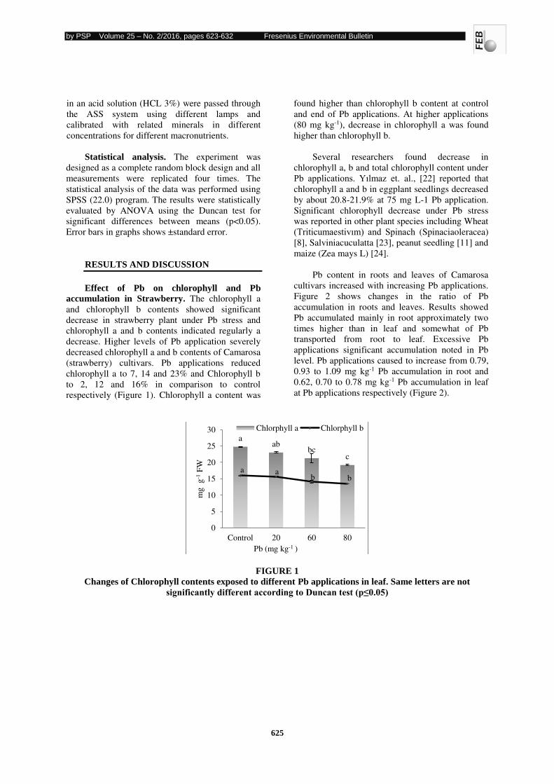
by PSP Volume 25 – No. 2/2016, pages 623-632 Fresenius Environmental Bulletin
625
in an acid solution (HCL 3%) were passed through
the ASS system using different lamps and
calibrated with related minerals in different
concentrations for different macronutrients.
Statistical analysis. The experiment was
designed as a complete random block design and all
measurements were replicated four times. The
statistical analysis of the data was performed using
SPSS (22.0) program. The results were statistically
evaluated by ANOVA using the Duncan test for
significant differences between means (p<0.05).
Error bars in graphs shows ±standard error.
RESULTS AND DISCUSSION
Effect of Pb on chlorophyll and Pb
accumulation in Strawberry. The chlorophyll a
and chlorophyll b contents showed significant
decrease in strawberry plant under Pb stress and
chlorophyll a and b contents indicated regularly a
decrease. Higher levels of Pb application severely
decreased chlorophyll a and b contents of Camarosa
(strawberry) cultivars. Pb applications reduced
chlorophyll a to 7, 14 and 23% and Chlorophyll b
to 2, 12 and 16% in comparison to control
respectively (Figure 1). Chlorophyll a content was
found higher than chlorophyll b content at control
and end of Pb applications. At higher applications
(80 mg kg-1), decrease in chlorophyll a was found
higher than chlorophyll b.
Several researchers found decrease in
chlorophyll a, b and total chlorophyll content under
Pb applications. Yılmaz et. al., [22] reported that
chlorophyll a and b in eggplant seedlings decreased
by about 20.8-21.9% at 75 mg L-1 Pb application.
Significant chlorophyll decrease under Pb stress
was reported in other plant species including Wheat
(Triticumaestivım) and Spinach (Spinaciaoleracea)
[8], Salviniacuculatta [23], peanut seedling [11] and
maize (Zea mays L) [24].
Pb content in roots and leaves of Camarosa
cultivars increased with increasing Pb applications.
Figure 2 shows changes in the ratio of Pb
accumulation in roots and leaves. Results showed
Pb accumulated mainly in root approximately two
times higher than in leaf and somewhat of Pb
transported from root to leaf. Excessive Pb
applications significant accumulation noted in Pb
level. Pb applications caused to increase from 0.79,
0.93 to 1.09 mg kg-1 Pb accumulation in root and
0.62, 0.70 to 0.78 mg kg-1 Pb accumulation in leaf
at Pb applications respectively (Figure 2).
FIGURE 1
Changes of Chlorophyll contents exposed to different Pb applications in leaf. Same letters are not
significantly different according to Duncan test (p≤0.05)
aab
bcc
a ab b
0
5
10
15
20
25
30
Control 20 60 80
mg
g-1
FW
Pb (mg kg-1 )
Chlorphyll a Chlorphyll b
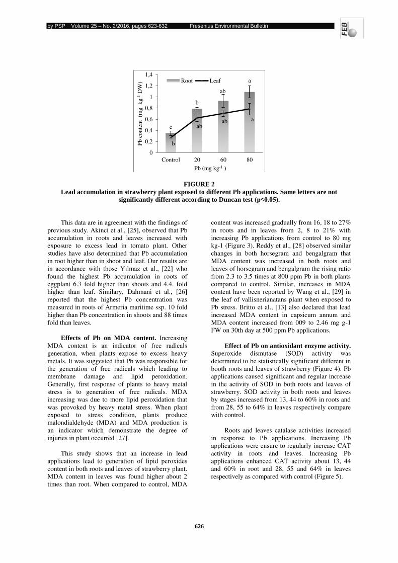
by PSP Volume 25 – No. 2/2016, pages 623-632 Fresenius Environmental Bulletin
626
FIGURE 2
Lead accumulation in strawberry plant exposed to different Pb applications. Same letters are not
significantly different according to Duncan test (p≤0.05).
This data are in agreement with the findings of
previous study. Akinci et al., [25], observed that Pb
accumulation in roots and leaves increased with
exposure to excess lead in tomato plant. Other
studies have also determined that Pb accumulation
in root higher than in shoot and leaf. Our results are
in accordance with those Yılmaz et al., [22] who found the highest Pb accumulation in roots of
eggplant 6.3 fold higher than shoots and 4.4. fold
higher than leaf. Similary, Dahmani et al., [26]
reported that the highest Pb concentration was
measured in roots of Armeria maritime ssp. 10 fold
higher than Pb concentration in shoots and 88 times
fold than leaves.
Effects of Pb on MDA content. Increasing
MDA content is an indicator of free radicals
generation, when plants expose to excess heavy
metals. It was suggested that Pb was responsible for
the generation of free radicals which leading to
membrane damage and lipid peroxidation.
Generally, first response of plants to heavy metal
stress is to generation of free radicals. MDA
increasing was due to more lipid peroxidation that
was provoked by heavy metal stress. When plant
exposed to stress condition, plants produce
malondialdehyde (MDA) and MDA production is
an indicator which demonstrate the degree of
injuries in plant occurred [27].
This study shows that an increase in lead
applications lead to generation of lipid peroxides
content in both roots and leaves of strawberry plant.
MDA content in leaves was found higher about 2
times than root. When compared to control, MDA
content was increased gradually from 16, 18 to 27%
in roots and in leaves from 2, 8 to 21% with
increasing Pb applications from control to 80 mg
kg-1 (Figure 3). Reddy et al., [28] observed similar
changes in both horsegram and bengalgram that
MDA content was increased in both roots and
leaves of horsegram and bengalgram the rising ratio
from 2.3 to 3.5 times at 800 ppm Pb in both plants
compared to control. Similar, increases in MDA
content have been reported by Wang et al., [29] in
the leaf of vallisnerianatans plant when exposed to
Pb stress. Britto et al., [13] also declared that lead
increased MDA content in capsicum annum and
MDA content increased from 009 to 2.46 mg g-1
FW on 30th day at 500 ppm Pb applications.
Effect of Pb on antioxidant enzyme activity.
Superoxide dismutase (SOD) activity was
determined to be statistically significant different in
booth roots and leaves of strawberry (Figure 4). Pb
applications caused significant and regular increase
in the activity of SOD in both roots and leaves of
strawberry. SOD activity in both roots and leaves
by stages increased from 13, 44 to 60% in roots and
from 28, 55 to 64% in leaves respectively compare
with control.
Roots and leaves catalase activities increased
in response to Pb applications. İncreasing Pb applications were ensure to regularly increase CAT
activity in roots and leaves. Increasing Pb
applications enhanced CAT activity about 13, 44
and 60% in root and 28, 55 and 64% in leaves
respectively as compared with control (Figure 5).
c
b
ab
a
b
abab a
0
0,2
0,4
0,6
0,8
1
1,2
1,4
Control 20 60 80
Pb
co
nte
nt
(m
g
kg
-1D
W)
Pb (mg kg-1 )
Root Leaf
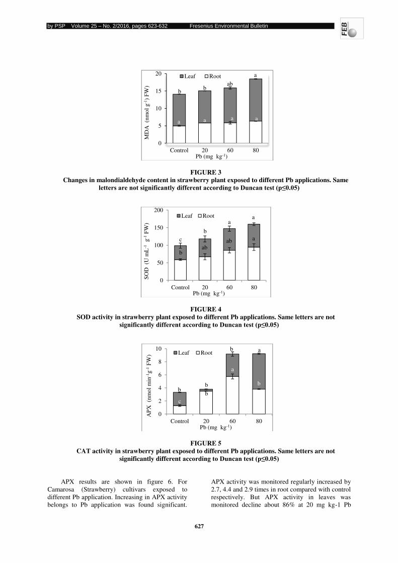
by PSP Volume 25 – No. 2/2016, pages 623-632 Fresenius Environmental Bulletin
627
FIGURE 3
Changes in malondialdehyde content in strawberry plant exposed to different Pb applications. Same
letters are not significantly different according to Duncan test (p≤0.05)
FIGURE 4
SOD activity in strawberry plant exposed to different Pb applications. Same letters are not
significantly different according to Duncan test (p≤0.05)
FIGURE 5
CAT activity in strawberry plant exposed to different Pb applications. Same letters are not
significantly different according to Duncan test (p≤0.05)
APX results are shown in figure 6. For
Camarosa (Strawberry) cultivars exposed to
different Pb application. Increasing in APX activity
belongs to Pb application was found significant.
APX activity was monitored regularly increased by
2.7, 4.4 and 2.9 times in root compared with control
respectively. But APX activity in leaves was
monitored decline about 86% at 20 mg kg-1 Pb
a a a a
bb
ab
a
0
5
10
15
20
Control 20 60 80M
DA
(n
mo
l g
-1)
FW
)
Pb (mg kg-1)
Leaf Root
bab
ab ac
b
aa
0
50
100
150
200
Control 20 60 80
SO
D
(U m
L-1
g-1
FW
)
Pb (mg kg-1)
Leaf Root
c
b
a
bb
b
b a
0
2
4
6
8
10
Control 20 60 80
AP
X (n
mo
l m
in-1
g-1
FW
)
Pb (mg kg-1)
Leaf Root
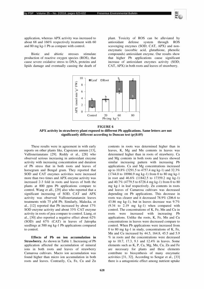
by PSP Volume 25 – No. 2/2016, pages 623-632 Fresenius Environmental Bulletin
628
application, whereas APX activity was increased to
about 68 and 166% respectively treatment with 60
and 80 mg kg-1 Pb as compare with control.
Biotic and abiotic stresses stimulate
production of reactive oxygen species (ROS), that
cause severe oxidative stress to DNA, proteins and
lipids damage and eventually causing the death of
plant. Toxicity of ROS can be alleviated by
antioxidant defense system through ROS
scavenging enzymes (SOD; CAT, APX) and non-
enzymatic (ascorbic acid, glutathione, phenolic
compounds) antioxidant enzyme. Our results show
that higher Pb applications cause significant
increase of antioxidant enzymes activity (SOD;
CAT, APX) in both roots and leaves of strawberry.
FIGURE 6
APX activity in strawberry plant exposed to different Pb applications. Same letters are not
significantly different according to Duncan test (p≤0.05)
These results were in agreement in with early
reports on other plants like, Capsicum annum [13],
Vallisnerianatans [29]. Reddy et al., [28] who
observed serious increasing in antioxidant enzyme
activity with increasing concentration and duration
of Pb stress that in both roots and leaves of
horsegram and Bengal gram. They reported that
SOD and CAT enzymes activities were increased
more than two times and APX enzyme activity was
increased 2-3 fold in roots and leaves of both the
plants at 800 ppm Pb applications compare to
control. Wang et all., [29] also who reported that a
significant increasing of SOD, CAT and APX
activity was observed Vallisnerianatansin leaves
treatments with 75 µM Pb. Similarly, Malecka, et
al., [12] reported that Pb increased by about 17%
SOD enzyme activity and about 33% CAT enzyme
activity in roots of pea compare to control. Liang, et
al., [30] also reported a negative effect about 62%
(SOD) and 67% (CAT) in leaves of Jatropha
seedlings at 500 mg kg-1 Pb applications compared
to control.
Effects of Pb on ion accumulation in
Strawberry. As shown in Table 1. Increasing of Pb
application affected the accumulation of mineral
ions in both roots and leaves of strawberry
Camarosa cultivars. Macro ion accumulation was
found higher than micro ion accumulation in both
roots and leaves. Contrarily, Ca, Fe, Cu and Zn
contents in roots was determined higher than in
leaves, K, Mg and Mn contents in leaves was
determined higher than in roots of strawberry. Ca
and Mg contents in both roots and leaves showed
similar increasing pattern with increasing Pb
applications. Ca and Mg concentrations increased
up to 10.8% (3291.5 to 4757.4 mg kg-1) and 32.3%
(1744.0 to 18986.9 mg kg-1) from 0 to 80 mg kg-1
in root and 46.6% (11842.5 to 17359.2 mg kg-1)
and 40.7% (4779.5 to 6728.4 mg kg-1) from 0 to 80
mg kg-1 in leaf respectively. Zn contents in roots
and leaves of Camarosa cultivars was decreased
depending on Pb applications. This decrease in
roots was clearer and it decreased 78.9% (206.6 to
43.86 mg kg-1), but in leaves decrease was 9.7%
(9.34 to 2.19 mg kg-1) when compared with
control. The concentrations of K, Fe, Mn and Cu in
roots were increased with increasing Pb
applications. Unlike the roots, K, Fe, Mn and Cu
concentrations in leaves were decreased compare to
control. When Pb applications were increased from
0 to 80 mg kg-1 in study, concentrations of K, Fe,
Mn and Cu increased by 44.5, 164.8, 45.5 and 5.9
% in roots and the concentrations were decreased
up to 10.7, 17.3, 9.1 and 12.4% in leaves. Some
elements such as K, P, Ca, Mg, Mn, Cu, Zn and Fe
are necessary for plants and these elements
contribute to biosynthesis of many enzymatic
activities [31, 32]. According to Sengar et al., [33]
there is a antagonistic effect among nutrient uptake
c
b
a
bb
b
b a
0
2
4
6
8
10
Control 20 60 80
AP
X (n
mo
l m
in-1
g-1
FW
)
Pb (mg kg-1)
Leaf Root
by PSP Volume 25 – No. 2/2016, pages 623-632 Fresenius Environmental Bulletin
629
and heavy metal stress in plants and changes in
mineral nutrition may occur from blockage of roots
absorption, a decrease in translocation processes, or
by competition between ions, impairing critical
physiological processes [4]. Many researchers
decelerated that Pb have a negative effect of
nutrition uptake and these effect were shown
widely in different plant species and cultivars.
Kibria et al., [34] found similar results in spinach
plant. Who reported that Pb decreased potassium
and magnesium concentration in both roots and
shoots but Zinc and iron concentration decreased
only in roots with increasing Pb level. On the
contrary increasing Pb level increased manganese
concentration (in both roots and shoots), nitrogen
and magnesium concentrations (in shoots) and
calcium concentration (in root) in spinach.
Lamhamdi et al., [8] also reported that Pb decreased
the uptake of Na, K, Ca, P, Mg, Cu and Zn,
Although Mn concentration is increased in wheat
and spinach. Similar study reported in various plant
species increasing Pb applications generally
inhibited the uptake of all mineral elements in
tomato [25], eggplant seedling [22], canola [35] and
azolacaroliniana- Anabaena [36].
In conclusion, our research indicated that
higher levels of Pb could be accumulated in both
roots and leaves of strawberry plant. The
accumulation of Pb in roots was higher than leaves
because root is the first organ exposed to Pb and
could be expanded to prevent translocation of
higher amount of Pb in shoots. Pb accumulation
reduced chlorophyll a and chlorophyll b and
proportional decrease of chlorophyll a was found
higher than chlorophyll b with increasing Pb
applications from 20 mg kg-1 to 80 mg kg-1. The
decreased chlorophyll content caused reduction of
growth because of α-amino laevulinate
dehydrogenase is strongly inhibited by Pb ions and
this enzyme has a key role for chlorophyll
biosynthesis [37]. Treatments with Pb caused
oxidative stress as namely increased lipid peroxide
content induces the production free radicals. The
defense mechanism of strawberry against Pb
applications triggered the production of some
protective mechanism (antioxidant enzyme) such as
increased SOD, CAT and APX activities were
increased with increasing Pb concentrations. In
addition, excess Pb applications were seriously
blocked to nutrition uptake. These results ensure an
important mark for understanding the change of
chlorophyll content in leaves, accumulation of Pb
and defense mechanisms of strawberry plant in both
roots and leaves.
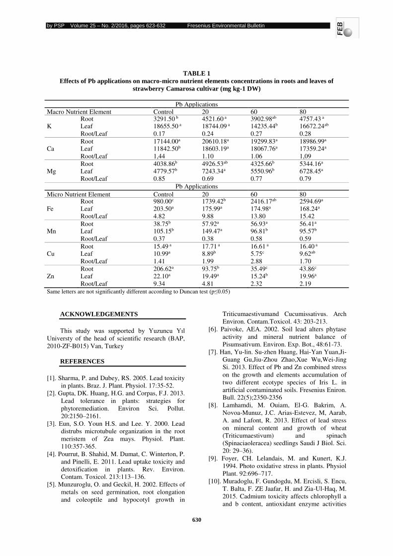
by PSP Volume 25 – No. 2/2016, pages 623-632 Fresenius Environmental Bulletin
630
TABLE 1
Effects of Pb applications on macro-micro nutrient elements concentrations in roots and leaves of
strawberry Camarosa cultivar (mg kg-1 DW)
Pb Applications Macro Nutrient Element Control 20 60 80 Root 3291.50 b 4521.60 a 3902.98ab 4757.43 a K Leaf 18655.50 a 18744.09 a 14235.44b 16672.24ab
Root/Leaf 0.17 0.24 0.27 0.28
Root 17144.00a 20610.18a 19299.83a 18986.99a Ca Leaf 11842.50b 18603.19a 18067.76a 17359.24a
Root/Leaf 1,44 1.10 1.06 1,09
Root 4038.86b 4926.53ab 4325.66b 5344.16a Mg Leaf 4779.57b 7243.34a 5550.96b 6728.45a Root/Leaf 0.85 0.69 0.77 0.79
Pb Applications
Micro Nutrient Element Control 20 60 80 Root 980.00c 1739.42b 2416.17ab 2594.69a Fe Leaf 203.50a 175.99a 174.98a 168.24a
Root/Leaf 4.82 9.88 13.80 15.42
Root 38.75b 57.92a 56.93a 56.41a Mn Leaf 105.15b 149.47a 96.81b 95.57b
Root/Leaf 0.37 0.38 0.58 0.59
Root 15.49 a 17.71 a 16.61 a 16.40 a Cu Leaf 10.99a 8.89b 5.75c 9.62ab
Root/Leaf 1.41 1.99 2.88 1.70
Root 206.62a 93.75b 35.49c 43.86c Zn Leaf 22.10a 19.49a 15.24b 19.96a
Root/Leaf 9.34 4.81 2.32 2.19
Same letters are not significantly different according to Duncan test (p≤0.05)
ACKNOWLEDGEMENTS
This study was supported by Yuzuncu Yıl Universty of the head of scientific research (BAP,
2010-ZF-B015) Van, Turkey
REFERENCES
[1]. Sharma, P. and Dubey, RS. 2005. Lead toxicity
in plants. Braz. J. Plant. Physiol. 17:35-52.
[2]. Gupta, DK. Huang, H.G. and Corpas, F.J. 2013.
Lead tolerance in plants: strategies for
phytoremediation. Environ Sci. Pollut.
20:2150–2161.
[3]. Eun, S.O. Youn H.S. and Lee. Y. 2000. Lead
distrubs microtubule organization in the root
meristem of Zea mays. Physiol. Plant.
110:357-365.
[4]. Pourrut, B. Shahid, M. Dumat, C. Winterton, P.
and Pinelli, E. 2011. Lead uptake toxicity and
detoxification in plants. Rev. Environ.
Contam. Toxicol. 213:113–136.
[5]. Munzuroglu, O. and Geckil, H. 2002. Effects of
metals on seed germination, root elongation
and coleoptile and hypocotyl growth in
Triticumaestivumand Cucumissativus. Arch
Environ. Contam.Toxicol. 43: 203-213.
[6]. Paivoke, AEA. 2002. Soil lead alters phytase
activity and mineral nutrient balance of
Pisumsativum. Environ. Exp. Bot., 48:61-73.
[7]. Han, Yu-lin. Su-zhen Huang, Hai-Yan Yuan,Ji-
Guang Gu,Jiu-Zhou Zhao,Xue Wu,Wei-Jing
Si. 2013. Effect of Pb and Zn combined stress
on the growth and elements accumulation of
two different ecotype species of Iris L. in
artificial contaminated soils. Fresenius Eniron.
Bull. 22(5);2350-2356
[8]. Lamhamdi, M. Ouiam, El-G. Bakrim, A.
Novoa-Munuz, J.C. Arias-Estevez, M, Aarab,
A. and Lafont, R. 2013. Effect of lead stress
on mineral content and growth of wheat
(Triticumaestivum) and spinach
(Spinaciaoleracea) seedlings Saudi J Biol. Sci.
20: 29–36).
[9]. Foyer, CH. Lelandais, M. and Kunert, K.J.
1994. Photo oxidative stress in plants. Physiol
Plant. 92:696–717.
[10]. Muradoglu, F. Gundogdu, M. Ercisli, S. Encu,
T. Balta, F. ZE Jaafar, H. and Zia-Ul-Haq, M.
2015. Cadmium toxicity affects chlorophyll a
and b content, antioxidant enzyme activities
by PSP Volume 25 – No. 2/2016, pages 623-632 Fresenius Environmental Bulletin
631
and mineral nutrient accumulation in
strawberry. Biological Research 48:1-7.
[11]. Dogan, M. Akgul, H. Tozlu, I. 2013. Lead
accumulation and toxicity in peanut (Arachis
hypogaea L.) seedlings. Fresenius Environ.
Bull. 22 (8), 2350−2356. [12]. Malecka, A. Jarmuszkiewicz, W. and
Tomaszewska, B. 2001. Antioxidative defense
to lead stress in subcellular compartments of
pea root cells. Acta Bochimica Polonica,
48:687-698.
[13]. Britto, AJD. Sebastian S.R. and Gracelin, H.S.
2013. Effect of Lead on malondialdehyde,
superoxide dismutase, proline activity and
chlorophyll content in Capsicum annum.
Bioresearch Bulletin 2:1-5.
[14]. Anonymous: 2012. FAO
htpp://faostat.fao.org/site/339/default.aspx.
22-07-2015.
[15]. Anonymous: 2014.
http://rapory.tuik.gov.tr/20-07-2015.
[16]. Eltez, R.Z. and Tüzel, Y. 2007. The Effects of
different soilless culture techniques in “A-
Shape” system on the yield and quality of greenhouse strawberry production. Ege Üniv.
Fac. Agricult. J. 44:15-27.
[17]. Lichtentaler, HK. 1994. Chlorophyll and
carotenoids pigments of photosynthetic
biomembranes. Meth. Enzymol. 148:350–82.
[18]. Heath, R.L. and Packer, L. 1968.
Photoperoxidation in isolated chloroplast. I.
Kinetics and stoichiometry of fatty acid
peroxidation. Arch. Biochem Biophys.
125:189-198.
[19]. Giannopolitis, C.N. and Ries, S.K. 1977.
Superoxide dismutase. I. Occurrence in higher
plants. Plant Physiol59: 309-314.
[20]. Aebi, H. 1984. Catalase in vitro. Methods
Enzymol. 105,121–126.
[21]. Nakano, Y. and Asada, K. 1981. Hydrogen
peroxide is scavenged by ascorbate specific
peroxidase in spinach Chloroplasts. Plant Cell
Physiol. 22:867-880.
[22]. Yılmaz, K. Akıncı, İ.E. and Akıncı, S. 2009. Effect of lead accumulation on growth and
mineral composition of eggplant seedlings
(Solanummelongena). New Zealand J. Crop.
Hort. Sci. 37:189-199.
[23]. Phetsombat, S. Kruatrachue, M.
Pokethitiyook, P. and Upatham, S. 2006.
Toxicity and bioaccumulation of cadmium and
lead in Salviniacucullata. J. Enviro. Biolog.
27:645-652.
[24]. Ghani, A. 2010. Effect of lead on growth,
chlorophyll and lead (Pb+) contents of two
varieties of maize (Zea mays L.). Pak. J. Nutr.
9:887-891.
[25]. Akinci, İE. Akinci, S.and Yılmaz, K. 2010. Response of tomato (SolanumlycopersicumL.)
to lead toxicity: Growth, element uptake,
chlorophyll and water content. African J. Agri.
Res. 5:416-423.
[26]. Dahmani, M. Van-Oort, HF. Gelieand B. and
Balabane M. 2000. Strategies of heavy metal
uptake by three plant species growing near a
metal smelter. Enviro.Pollut.109:231-238.
[27]. Xu, W. Li, W. He, J. Balwant, S. and Xiong,
Z. 2009. Effect of insoluble Zn, Cd, and
EDTA on growth, activities of antioxidant
enzymes and uptake of Zn and Cd in
Vetiveriazizanioidies. J. Environ Sci. (China).
21:186-192.
[28]. Reddy, AM. Kumar, SG. Jyothsnakumari, G.
Thimmanaik, S. and Sudhakar, C. 2005. Lead
induced changes in antioxidant metabolism of
horsegram (Macrotylomauniflorum (Lam.)
Verdc.) and bengalgram (Cicerarietinum L.).
Chemosphere 60:97-104(2005).
[29]. Wang, P. Zhang, S. Whang, C. and Lu, J.
2012. Effect of Pb on the oxidative stress and
antioxidant response in a Pb bioaccumulator
plant vallisnerianatans. Ecotoxicology and
Environmental Safety. 78:28-34.
[30]. Liang, J. Yang, Z. Tang, L. Xu, Y. Wang, S.
and Chen, F. 2012. Growth performence and
tolerance responses of jatropha
(Jatrophacurcas) seedlings subjected to
isolated or combined cadmium and lead stress.
İnt. J. Agric. Biol. 14:861-869.
[31]. Van de Mortel, JA. Villanueva, LA. Schat, H.
Kwekkeboom, J. Coughlan, S. Moerland, P.D.
Van-Themaat, EVL. Koornneef, M. and Aarts,
MGM. 2006. Large expression differences in
genes for iron and zinc homeostasis, stress
response, and lignin biosynthesis distinguish
roots of Arabidopsis thaliana and the related
metal hyperaccumulator Thlaspicaerulescens.
Plant Physiol., 142:1127–1147.
[32]. Ali, M.B. Singh, N. Shohael, A.M., Hahn, E.J.
and Paek, K.Y. 2006. Phenolics metabolism
and lignin synthesis in root suspension
cultures of Panax ginseng in response to
copper stress.Plant Sci., 171:147–154.
[33]. Sengar, R.S. Gautam, M. Sengar, R.S. Garg,
S.K. Sengar, K. and Chaudhary, R. 2008. Lead
stress effects on physiobiochemical activities
of higher plants. Rev. Environ. Contam.
Toxicol. 196:73–93.
[34]. Kibria, M.G. Maniruzzaman, M. İslam, M. and Osman, K.T. 2010. Effect of soil-applied
lead on growth and partitioning of ion
concentration in Spinacea-oleracea L. tissues.
Soil & Environ. 29:1-6.

by PSP Volume 25 – No. 2/2016, pages 623-632 Fresenius Environmental Bulletin
632
[35]. Ashraf, M.Y. Azhar, N. Ashraf, M. Hussain,
M. and Arshad, M. 2011. Influence of lead on
growth and nutrient accumulation in canola
(Brassica napus L.) cultivars. J. Environ. Biol.
32:659-666.
[36]. Roberts, A.E. Boylen, CW. and Nierzwicki-
Bauer, SA. 2014. Effects of lead accumulation
on the Azollacaroliniana–Anabaena
association. Ecotox. Envir. Safe. 102:100–104.
[37]. Prasad, D.D.K. and Prasad, A.R.K. 1987.
Altered α-amino luvelinic acid metabolism by
Pb and Hg in germinating seedling of Bajra
(Pennisetumtyphoidenum). J. Plant. Physiol.
127:241–249.
Received: 04.09.2015
Accepted: 17.12.2015
CORRESPONDING AUTHOR
Ferhad Muradoğlu
Department of Horticulture
Faculty of Agriculture and Natural Sciences
Abant Izzet Baysal University
Bolu – TURKEY
e-mail: [email protected]
by PSP Volume 25 – No. 2/2016, pages 633-640 Fresenius Environmental Bulletin
633
INFLUENCE OF ALKALI CATALYSTS ON THE
SUPERCRITICAL WATER GASIFICATION OF
CYANOBACTERIA
Huiwen Zhanga, b, Wei Zhua, Miao Gonga, Yujie Fana
aCollege of Environment, Hohai University, P.R. China
bHohai University, College of Environment, Nanjing, Jiangsu, 210098, P.R. China
ABSTRACT
The paper focused on enhancing
hydrogen(H2) production by addition of alkali
catalysts, based on that cyanobacteria could be used
as a ideal feedstock of supercritical
gasification(SCWG). We studied the influence and
mechanism of alkali catalysts in the SCWG process
of cyanobacteria from the angle of loading and
types of alkali catalysts. Our results indicated that
some alkali catalysts could promote yield of H2 to a
great extent, the H2 yield reached 17.50 mol/kg dry
cyanobacteria at 500 oC, 22 MPa, 30 min and 5.0%
catalysts loading; two obvious stage features were
showed in the changing process of catalysts
loading: the enhancement of gas production and the
enhancement of H2 production; the catalysis of
promoting H2 production was determined by both
hydroxide ion and types of metal ions.
KEYWORDS:
alkali catalysts, supercritical water, gasification,
cyanobacteria
INTRODUCTION
Many academic and material resources have
been applied to control the widespread
eutrophication in the lakes of China, such as Taihu,
Dianchi, and Chaohu, is of great concern. However,
this phenomenon leads to the large-scale outbreak
of Cyanobacteria every year as before. Salvage has
become a conventional measure of treating
Cyanobacteria accumulated on the water surface. In
2010, about 100 boats were used and 670 000 t
Cyanobacteria slurry were captured [1].
Cyanobacteria slurry is characterized by numerous
microcystis cells as well as high moisture, organic
matter, N, and P contents.
The engineering technology of cyanobacteria
was mostly built on dewatering operation, which
would consume a mass of time and work in the
process. Due to the high water content of
cyanobacteria, the anaerobic fermentation and
thermal treatment results in low treatment
efficiency and engineering value. Given the
properties of dissolving capacity and oxidbillity of
organic matters in supercritical water, SCWG
technology has been extensively used to treat wet
biomass with characteristics of high moisture and
organic matter content, which can provide
sufficient water and high solubility to get
supercritical status. Nature changes harmful organic
matter into stable products. Thus, clean and
efficient H2 energy is produced, and waste
treatment and energy utilization are achieved.
Accordingly, supercritical gasification has been
widely applied in waste biomass processing and
utilization, including municipal sludge [2-5],
kitchen waste [6-8], sawdust, and agricultural straw
[9,10]. Thus, SCWG technology was a possible
option to achieve cyanobacteria processing and
utilization.
Due to the extreme operating conditions of
SCWG, catalysts addition had been studied and
applied at lower reaction temperature and pressure.
Alkali catalysts with high catalytic efficiency had
been known in the early 1940 s by researchers.
Elliott et al.[11-13] firstly did research about effects
of alkali catalysts on the water gas shift reaction.
On the base of Elliot’s study, combined with catalysis effects of KOH on pyrocatechol and
glucose, Kruse et al.[14, 15] presented the chemical
equation as (1-5) to (1-8). It’s also considered that NaOH addition inhabited coke production, and
enhanced gas production of sewage sludge during
the process of SCWG in Zhang et al.’s studies[16].Watanabe et al.[17] used lignin as the
feedstocks of SCWG, NaOH addition increased 4
times of H2 yield.
NaOH、KOH、Ca(OH)2、Na2CO3、K2CO3 and
NaHCO3 were selected as catalysts in the SCWG
of glucose in Muangrat’s study[21], it’s found that these materials could enhance gas and H2
productions to some extent, the sequence of
catalytic effects on H2 production was listed as
follow: NaOH > KOH > Ca(OH)2 > K2CO3 >
Na2CO3 > NaHCO3, the salt basicity of
intermediates containing alkali metal ions was
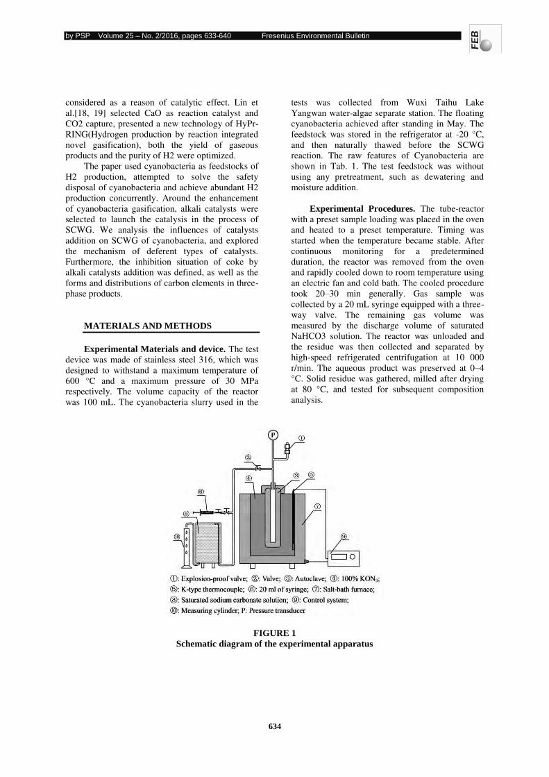
by PSP Volume 25 – No. 2/2016, pages 633-640 Fresenius Environmental Bulletin
634
considered as a reason of catalytic effect. Lin et
al.[18, 19] selected CaO as reaction catalyst and
CO2 capture, presented a new technology of HyPr-
RING(Hydrogen production by reaction integrated
novel gasification), both the yield of gaseous
products and the purity of H2 were optimized.
The paper used cyanobacteria as feedstocks of
H2 production, attempted to solve the safety
disposal of cyanobacteria and achieve abundant H2
production concurrently. Around the enhancement
of cyanobacteria gasification, alkali catalysts were
selected to launch the catalysis in the process of
SCWG. We analysis the influences of catalysts
addition on SCWG of cyanobacteria, and explored
the mechanism of deferent types of catalysts.
Furthermore, the inhibition situation of coke by
alkali catalysts addition was defined, as well as the
forms and distributions of carbon elements in three-
phase products.
MATERIALS AND METHODS
Experimental Materials and device. The test
device was made of stainless steel 316, which was
designed to withstand a maximum temperature of
600 °C and a maximum pressure of 30 MPa
respectively. The volume capacity of the reactor
was 100 mL. The cyanobacteria slurry used in the
tests was collected from Wuxi Taihu Lake
Yangwan water-algae separate station. The floating
cyanobacteria achieved after standing in May. The
feedstock was stored in the refrigerator at -20 °C,
and then naturally thawed before the SCWG
reaction. The raw features of Cyanobacteria are
shown in Tab. 1. The test feedstock was without
using any pretreatment, such as dewatering and
moisture addition.
Experimental Procedures. The tube-reactor
with a preset sample loading was placed in the oven
and heated to a preset temperature. Timing was
started when the temperature became stable. After
continuous monitoring for a predetermined
duration, the reactor was removed from the oven
and rapidly cooled down to room temperature using
an electric fan and cold bath. The cooled procedure
took 20–30 min generally. Gas sample was
collected by a 20 mL syringe equipped with a three-
way valve. The remaining gas volume was
measured by the discharge volume of saturated
NaHCO3 solution. The reactor was unloaded and
the residue was then collected and separated by
high-speed refrigerated centrifugation at 10 000
r/min. The aqueous product was preserved at 0–4
°C. Solid residue was gathered, milled after drying
at 80 °C, and tested for subsequent composition
analysis.
FIGURE 1
Schematic diagram of the experimental apparatus
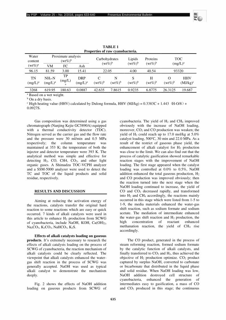
by PSP Volume 25 – No. 2/2016, pages 633-640 Fresenius Environmental Bulletin
635
Gas composition was determined using a gas
chromatograph (Nanjing Kejie GC5890A) equipped
with a thermal conductivity detector (TDC).
Nitrogen served as the carrier gas and the flow rate
and the pressure were 30 ml/min and 0.5 MPa
respectively; the column temperature was
maintained at 353 K; the temperature of both the
injector and detector temperature were 393 K. The
analytical method was simple and effective for
detecting H2, CO, CH4, CO2, and other light
organic gases. A Shimadzu TOC-VCPH analyzer
and a SSM-5000 analyzer were used to detect the
TC and TOC of the liquid products and solid
residue, respectively.
RESULTS AND DISCUSSION
Aiming at reducing the activation energy of
the reactions, catalysts transfer the original hard
reaction to some reactions which are easy or quick
occurred. 7 kinds of alkali catalysts were used in
this article to enhance H2 production from SCWG
of cyanobacteria, include NaOH, KOH, Ca(OH)2,
Na2CO3, K2CO3, NaHCO3, K2S.
Effects of alkali catalysts loading on gaseous
products. It’s extremely necessary to research the effects of alkali catalysts loading on the process of
SCWG of cyanobacteria, the reaction mechanism of
alkali catalysts could be clearly reflected. The
viewpoint that alkali catalysts enhanced the water-
gas shift reaction in the process of SCWG was
generally accepted. NaOH was used as typical
alkali catalyst to demonstrate the mechanism
deeply.
Fig. 2 shows the effects of NaOH addition
loading on gaseous products from SCWG of
cyanobacteria. The yield of H2 and CH4 improved
obviously with the increase of NaOH loading,
moreover, CO2 and CO production was weaken; the
yield of H2 could reach up to 17.0 mol/kg at 5.0%
catalyst loading, 500oC, 30 min and 22.0 MPa. As a
result of the restrict of gaseous phase yield, the
enhancement of alkali catalyst for H2 production
was close to the limit. We can also find out that the
process of catalytic gasification showed remarkable
reaction stages with the improvement of NaOH
loading. The first stage appeared when the catalyst
loading was controlled at 0.0% to 0.5%, NaOH
addition enhanced the total gaseous production, H2
and CO production was improved obviously; then
the reaction turned into the next stage when the
NaOH loading continued to increase, the yield of
CO and CO2 decreased rapidly, and transformed
into H2 and CH4 accordingly, the reactions mainly
occurred in this stage which were listed from 1-5 to
1-9, the media materials enhanced the water-gas
shift reaction, such as sodium formate and sodium
acetate. The mediation of intermediate enhanced
the water-gas shift reaction and H2 production, the
high concentration of reactant enhanced
methanation reaction, the yield of CH4 rise
accordingly.
The CO product, generated in the process of
steam reforming reaction, formed sodium formate
by the catalytic function of alkali catalysts, and
finally transferred to CO2 and H2, thus achieved the
objective of H2 production optimize. CO2 product
captured by surplus NaOH, converted to carbonate
or bicarbonate that distributed in the liquid phase
and solid residue. When NaOH loading was low,
NaOH addition destroyed cell structure of
cyanobacteria, enhanced the generation of
intermediates easy to gasification, a mass of CO
and CO2 produced in this stage; the continuous
TABLE 1
Properties of raw cyanobacteria.
Water
content
(wt%)a
Proximate analysis
(wt%)b Carbohydrates
(wt%)b
Lipids
(wt%)b
Proteins
(wt%)b
TOC
(mg/L)a
VM FC Ash
96.15 81.59 3.00 15.41 22.05 4.00 40.54 93320
TN
(mg/L)a
NH3-N
(mg/L)a
TP
(mg/L)a
DRP
(mg/L)a
C
(wt%)b
N
(wt%)b
S
(wt%)b
H
(wt%)b
O
(wt%)b
HHV
(MJ/kg)c
3268 619.95 180.63 0.0887 42.635 7.8615 0.9235 6.8775 26.3125 19.687 a Based on a wet weight.
b On a dry basis.
c High heating value (HHV) calculated by Dulong formula, HHV (MJ/kg) = 0.3383C + 1.443 H-O/8 +
0.0927S.
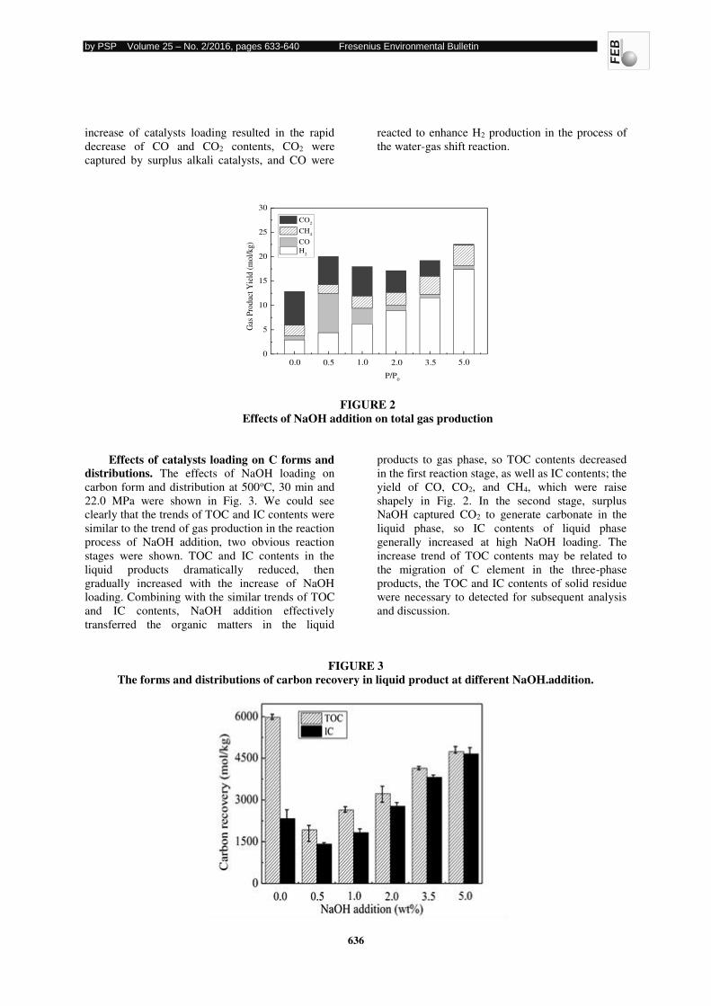
by PSP Volume 25 – No. 2/2016, pages 633-640 Fresenius Environmental Bulletin
636
increase of catalysts loading resulted in the rapid
decrease of CO and CO2 contents, CO2 were
captured by surplus alkali catalysts, and CO were
reacted to enhance H2 production in the process of
the water-gas shift reaction.
FIGURE 2
Effects of NaOH addition on total gas production
Effects of catalysts loading on C forms and
distributions. The effects of NaOH loading on
carbon form and distribution at 500oC, 30 min and
22.0 MPa were shown in Fig. 3. We could see
clearly that the trends of TOC and IC contents were
similar to the trend of gas production in the reaction
process of NaOH addition, two obvious reaction
stages were shown. TOC and IC contents in the
liquid products dramatically reduced, then
gradually increased with the increase of NaOH
loading. Combining with the similar trends of TOC
and IC contents, NaOH addition effectively
transferred the organic matters in the liquid
products to gas phase, so TOC contents decreased
in the first reaction stage, as well as IC contents; the
yield of CO, CO2, and CH4, which were raise
shapely in Fig. 2. In the second stage, surplus
NaOH captured CO2 to generate carbonate in the
liquid phase, so IC contents of liquid phase
generally increased at high NaOH loading. The
increase trend of TOC contents may be related to
the migration of C element in the three-phase
products, the TOC and IC contents of solid residue
were necessary to detected for subsequent analysis
and discussion.
FIGURE 3
The forms and distributions of carbon recovery in liquid product at different NaOH.addition.
0
5
10
15
20
25
30
0.0 0.5 1.0 2.0 3.5 5.0
Gas
Pro
du
ct Y
ield
(m
ol/
kg
)
P/P0
CO2
CH4
CO
H2
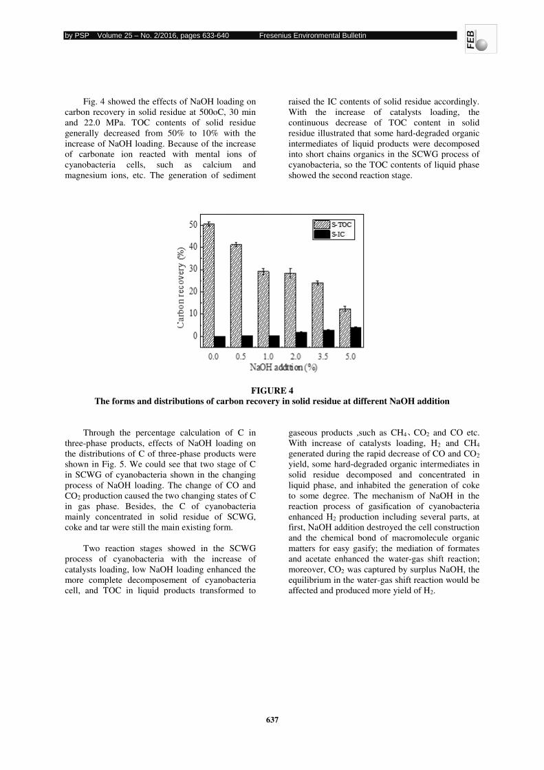
by PSP Volume 25 – No. 2/2016, pages 633-640 Fresenius Environmental Bulletin
637
Fig. 4 showed the effects of NaOH loading on
carbon recovery in solid residue at 500oC, 30 min
and 22.0 MPa. TOC contents of solid residue
generally decreased from 50% to 10% with the
increase of NaOH loading. Because of the increase
of carbonate ion reacted with mental ions of
cyanobacteria cells, such as calcium and
magnesium ions, etc. The generation of sediment
raised the IC contents of solid residue accordingly.
With the increase of catalysts loading, the
continuous decrease of TOC content in solid
residue illustrated that some hard-degraded organic
intermediates of liquid products were decomposed
into short chains organics in the SCWG process of
cyanobacteria, so the TOC contents of liquid phase
showed the second reaction stage.
FIGURE 4
The forms and distributions of carbon recovery in solid residue at different NaOH addition
Through the percentage calculation of C in
three-phase products, effects of NaOH loading on
the distributions of C of three-phase products were
shown in Fig. 5. We could see that two stage of C
in SCWG of cyanobacteria shown in the changing
process of NaOH loading. The change of CO and
CO2 production caused the two changing states of C
in gas phase. Besides, the C of cyanobacteria
mainly concentrated in solid residue of SCWG,
coke and tar were still the main existing form.
Two reaction stages showed in the SCWG
process of cyanobacteria with the increase of
catalysts loading, low NaOH loading enhanced the
more complete decomposement of cyanobacteria
cell, and TOC in liquid products transformed to
gaseous products ,such as CH4、CO2 and CO etc.
With increase of catalysts loading, H2 and CH4
generated during the rapid decrease of CO and CO2
yield, some hard-degraded organic intermediates in
solid residue decomposed and concentrated in
liquid phase, and inhabited the generation of coke
to some degree. The mechanism of NaOH in the
reaction process of gasification of cyanobacteria
enhanced H2 production including several parts, at
first, NaOH addition destroyed the cell construction
and the chemical bond of macromolecule organic
matters for easy gasify; the mediation of formates
and acetate enhanced the water-gas shift reaction;
moreover, CO2 was captured by surplus NaOH, the
equilibrium in the water-gas shift reaction would be
affected and produced more yield of H2.

by PSP Volume 25 – No. 2/2016, pages 633-640 Fresenius Environmental Bulletin
638
FIGURE 5
Effects of NaOH addition on the distribution of Carbon of Cyanobacteria in three-phase products.
Effects of alkali catalysts types on SCWG. Fig. 6 showed effects of alkali catalysts types on the
gas phase from SCWG of cyanobacteria at 500oC,
30 min , 22.0 MPa and 5.0% of catalysts loading.
The left figure illustrated effects of alkali catalysts
addition on gaseous products production, including
H2, CO and CH4, etc. Consider this from H2
production, not all types of alkali catalysts could
enhance H2 production from SCWG of
cyanobacteria, we sorted the H2 production
enhancement abilities of alkali catalyst as follow:
NaOH > KOH > Ca(OH)2 > Na2CO3 > K2CO3 >
NaHCO3 > K2S; combined with changing CO2
production showing in the right figure, Na2CO3 and
K2CO3 could achieve a relatively higher total gas
yield than NaOH and KOH addition, but CO2
contents accounted a higher percentage and the
yield of H2 was relatively lower. NaOH and KOH
could capture the generated CO2 and enhanced the
right shift of water-gas shift reaction, more and
more CO and H2O reacted to generate H2 and CO2,
surplus hydroxyl ion further reduced CO2 contents
in gaseous products. The yields of total gas and H2
with Ca(OH)2 additions were far below than NaOH
and KOH additions, it’s mainly because of different types of metal ions generated different types of
formate and acetate, the chemical potential energies
of these intermediates were of large difference,
some intermediates were hardly to degrade for
catalysis gasification, including calcium formate,
calcium acetate and calcium carbonate etc. To some
extent, the phenomenon of catalysis failure
emerged in the gasification process of
cyanobacteria. The differences of alkali catalysts
were determined by both hydroxyl ions and metal
ions in the process of SCWG.
In addition, we sorted the enhancement of CH4
production as follow: Na2CO3 >NaOH > K2CO3 >
KOH, the CH4 production mainly generated in
methanation reaction which occurred in the late
reaction process of SCWG. Both CO and CO2
could combined with H2 to produce CH4 and H2O,
the contents of CO, CO2 and H2 determined final
CH4 contents in gas phase.
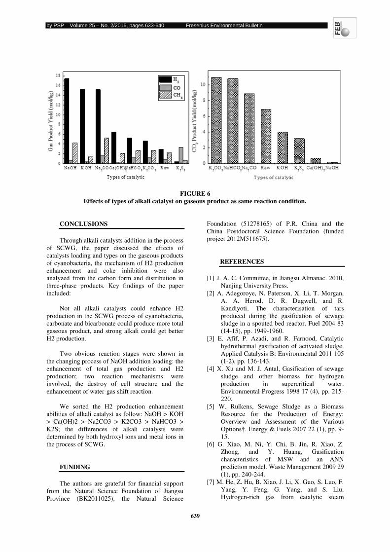
by PSP Volume 25 – No. 2/2016, pages 633-640 Fresenius Environmental Bulletin
639
FIGURE 6
Effects of types of alkali catalyst on gaseous product as same reaction condition.
CONCLUSIONS
Through alkali catalysts addition in the process
of SCWG, the paper discussed the effects of
catalysts loading and types on the gaseous products
of cyanobacteria, the mechanism of H2 production
enhancement and coke inhibition were also
analyzed from the carbon form and distribution in
three-phase products. Key findings of the paper
included:
Not all alkali catalysts could enhance H2
production in the SCWG process of cyanobacteria,
carbonate and bicarbonate could produce more total
gaseous product, and strong alkali could get better
H2 production.
Two obvious reaction stages were shown in
the changing process of NaOH addition loading: the
enhancement of total gas production and H2
production; two reaction mechanisms were
involved, the destroy of cell structure and the
enhancement of water-gas shift reaction.
We sorted the H2 production enhancement
abilities of alkali catalyst as follow: NaOH > KOH
> Ca(OH)2 > Na2CO3 > K2CO3 > NaHCO3 >
K2S; the differences of alkali catalysts were
determined by both hydroxyl ions and metal ions in
the process of SCWG.
FUNDING
The authors are grateful for financial support
from the Natural Science Foundation of Jiangsu
Province (BK2011025), the Natural Science
Foundation (51278165) of P.R. China and the
China Postdoctoral Science Foundation (funded
project 2012M511675).
REFERENCES
[1] J. A. C. Committee, in Jiangsu Almanac. 2010,
Nanjing University Press.
[2] A. Adegoroye, N. Paterson, X. Li, T. Morgan,
A. A. Herod, D. R. Dugwell, and R.
Kandiyoti, The characterisation of tars
produced during the gasification of sewage
sludge in a spouted bed reactor. Fuel 2004 83
(14-15), pp. 1949-1960.
[3] E. Afif, P. Azadi, and R. Farnood, Catalytic
hydrothermal gasification of activated sludge.
Applied Catalysis B: Environmental 2011 105
(1-2), pp. 136-143.
[4] X. Xu and M. J. Antal, Gasification of sewage
sludge and other biomass for hydrogen
production in supercritical water.
Environmental Progress 1998 17 (4), pp. 215-
220.
[5] W. Rulkens, Sewage Sludge as a Biomass
Resource for the Production of Energy:
Overview and Assessment of the Various
Options†. Energy & Fuels 2007 22 (1), pp. 9-
15.
[6] G. Xiao, M. Ni, Y. Chi, B. Jin, R. Xiao, Z.
Zhong, and Y. Huang, Gasification
characteristics of MSW and an ANN
prediction model. Waste Management 2009 29
(1), pp. 240-244.
[7] M. He, Z. Hu, B. Xiao, J. Li, X. Guo, S. Luo, F.
Yang, Y. Feng, G. Yang, and S. Liu,
Hydrogen-rich gas from catalytic steam
by PSP Volume 25 – No. 2/2016, pages 633-640 Fresenius Environmental Bulletin
640
gasification of municipal solid waste (MSW):
Influence of catalyst and temperature on yield
and product composition. International Journal
of Hydrogen Energy 2009 34 (1), pp. 195-203.
[8] J. A. Onwudili and P. T. Williams, Role of
sodium hydroxide in the production of
hydrogen gas from the hydrothermal
gasification of biomass. International Journal
of Hydrogen Energy 2009 34 (14), pp. 5645-
5656.
[9] T. Yoshida, Y. Oshima, and Y. Matsumura,
Gasification of biomass model compounds
and real biomass in supercritical water.
Biomass and Bioenergy 2004 26 (1), pp. 71-
78.
[10] Elliott, D.C., L.J. Sealock Jr, and R.S. Butner,
Aqueous catalyst systems for the water-gas
shift reaction. 3. Continuous gas processing
results. Industrial & Engineering Chemistry
Product Research and Development, 1986.
25(4): p. 541-549.
[11] Elliott, D.C. and L.J. Sealock Jr, Aqueous
catalyst systems for the water-gas shift
reaction. 1. Comparative catalyst studies.
Industrial & Engineering Chemistry Product
Research and Development, 1983. 22(3): p.
426-431.
[12] Elliott, D.C., R.T. Hallen, and L.J. Sealock Jr,
Aqueous catalyst systems for the water-gas
shift reaction. 2. Mechanism of basic catalysis.
Industrial & Engineering Chemistry Product
Research and Development, 1983. 22(3): p.
431-435.
[13] Sinag, A., A. Kruse, and R. Jens, Influence of
the Heating Rate and the Type of Catalyst on
the Formation of Key Intermediates and on the
Generation of Gases During Hydropyrolysis
of Glucose in Supercritical Water in a Batch
Reactor. Industrial & Engineering Chemistry
Research, 2004. 43(2): p. 502-508
[14] Kruse, A., et al., Gasification of Pyrocatechol
in Supercritical Water in the Presence of
Potassium Hydroxide. Industrial &
Engineering Chemistry Research, 2000.
39(12): p. 4842-4848.
[15] Zhang, Q.M., et al. Catalytic hydrogen
production from municipal sludge in
supercritical water with partial oxidation. in
International Conference on Power
Engineering (ICOPE-2007). 2007. Hangzhou,
PEOPLES R CHINA: Zhejiang Univ Press.
[16] Watanabe, M., et al., Catalytic effects of
NaOH and ZrO for partial oxidative
gasification of n-hexadecane and lignin in
supercritical water. Fuel, 2003. 82(5): p. 545-
552.
[17] Muangrat, R., J.A. Onwudili, and P.T.
Williams, Influence of alkali catalysts on the
production of hydrogen-rich gas from the
hydrothermal gasification of food processing
waste. Applied Catalysis B: Environmental,
2010. 100(3-4): p. 440-449.
[18] Lin, S.-Y., et al., Developing an innovative
method, HyPr-RING, to produce hydrogen
from hydrocarbons. Energy Conversion and
Management, 2002. 43(9-12): p. 1283-1290.
[19] Lin, S.-Y., et al., Hydrogen Production from
Hydrocarbon by Integration of Water Carbon
Reaction and Carbon Dioxide Removal
(HyPr-RING Method). Energy & Fuels, 2001.
15(2): p. 339-343.
Received: 28.09.2015
Accepted: 08.01.2016
CORRESPONDING AUTHOR
Huiwen Zhang
Hohai University
College of Environment
Nanjing, Jiangsu 210098 – P.R. CHINA.
e-mail: [email protected]
by PSP Volume 25 – No. 2/2016, pages 641-646 Fresenius Environmental Bulletin
641
RELATIONSHIPS BETWEEN SELECTED SOIL PROPERTIES
EXAMINED BY THE LUCAS PROJECT AND SATELLITE-
DERIVED VEGETATION INDICES FOR POLAND
Dariusz Gozdowski
Department of Experimental Design and Bioinformatics, Warsaw University of Life Sciences, Nowoursynowska 159, 02-776 Warsaw,
Poland
ABSTRACT
Satellite-derived data are a valuable source of
information about the spatial variability of soil at
regional scales. The aim of this study was to
evaluate the relationships between satellite-derived
vegetation indices and selected soil properties
obtained during the LUCAS Topsoil Survey. Soil
samples from cropland areas in Poland were
compared to low resolution, satellite-derived data.
The results showed significant correlations between
clay, silt and sand content and satellite-derived
vegetation indices and are promising for the
improvement of predictions soil texture at a
regional scale.
KEYWORDS: soil fractions, soil sampling, NDVI, EVI, correlations
INTRODUCTION
The prediction of soil properties, such as soil
organic carbon (SOC) content, soil texture (i.e.,
clay, silt and sand) and other variables that
characterize soil quality, is important at a regional
scale because of environmental issues. Low soil
organic matter, which is strongly correlated with
SOC, is one of the factors that accelerates the soil
erosion process [1], and another important factor
for soil erosion is soil texture, especially the
proportion of sand and clay. Therefore, monitoring
the spatial and temporal variability of these
properties is very important. These soil properties
are also critical for maintaining high and sustained
crop yields. High SOC and moderate clay content
increase soil productivity and mitigate soil erosion
and leaching. In Poland, nitrogen and phosphorus
leaching must be limited due to the eutrophication
of the Baltic Sea [2]. Areas with low SOC and clay
content should be mapped as they are vulnerable to
leaching.
High resolution mapping of SOC, soil texture
and other soil properties is not possible at a regional
scale because of high costs, so proximal sensing
methods are more commonly used and partly
replace soil sampling. One of valuable sources of
information about soil spatial variability is satellite
imagery. Soil properties are related to vegetation
indices, and many previous examinations have
proved the usefulness of satellite-derived variables
for the proximal sensing of some soil properties.
Poggio et al. [3] used various satellite data, e.g.,
MODIS (Moderate Resolution Imaging
Spectroradiometer), to distinguish between soils
with high or low soil organic matter, such as peat
soils vs. other soils. MODIS data and terrain
attributes were used by Dobos et al. [4] to delineate
soil parent material. Satellite data are also used as
ancillary data for the interpolation of the spatial
distribution of SOC [5, 6]; NDVI (Normalized
Difference Vegetation Index) is often used as a
covariate for predicting SOC. However, the
relationship between soil texture and satellite data
has rarely been examined. One study of soil texture
mapping using satellite imagery was conducted by
Liao et al. [7], and the authors showed that remote
sensing data significantly improves estimates of
surface soil texture
In most publications, satellite data are treated
as auxiliary variables to improve spatial
predictions. Such an approach is especially useful at
the regional scale where dense soil sampling is
impossible and proximal ground sensing methods,
such as electrical conductivity, are insufficient.
In the present study, the relationships between
selected soil properties (e.g., SOC, clay, silt and
sand content) examined by the LUCAS (Land
Use/Cover Area frame Statistical Survey) EU soil
project in 2009 [8] and MODIS data are examined
at a regional scale, i.e., the area of Poland.
MATERIAL AND METHODS
Soil data. For the analyses, soil sampling data
collected as part of the LUCAS Topsoil Survey [8]
were used. For all samples, the following soil
properties were measured: percentage of coarse
fragments, clay, silt and sand content, pH (in CaCl2
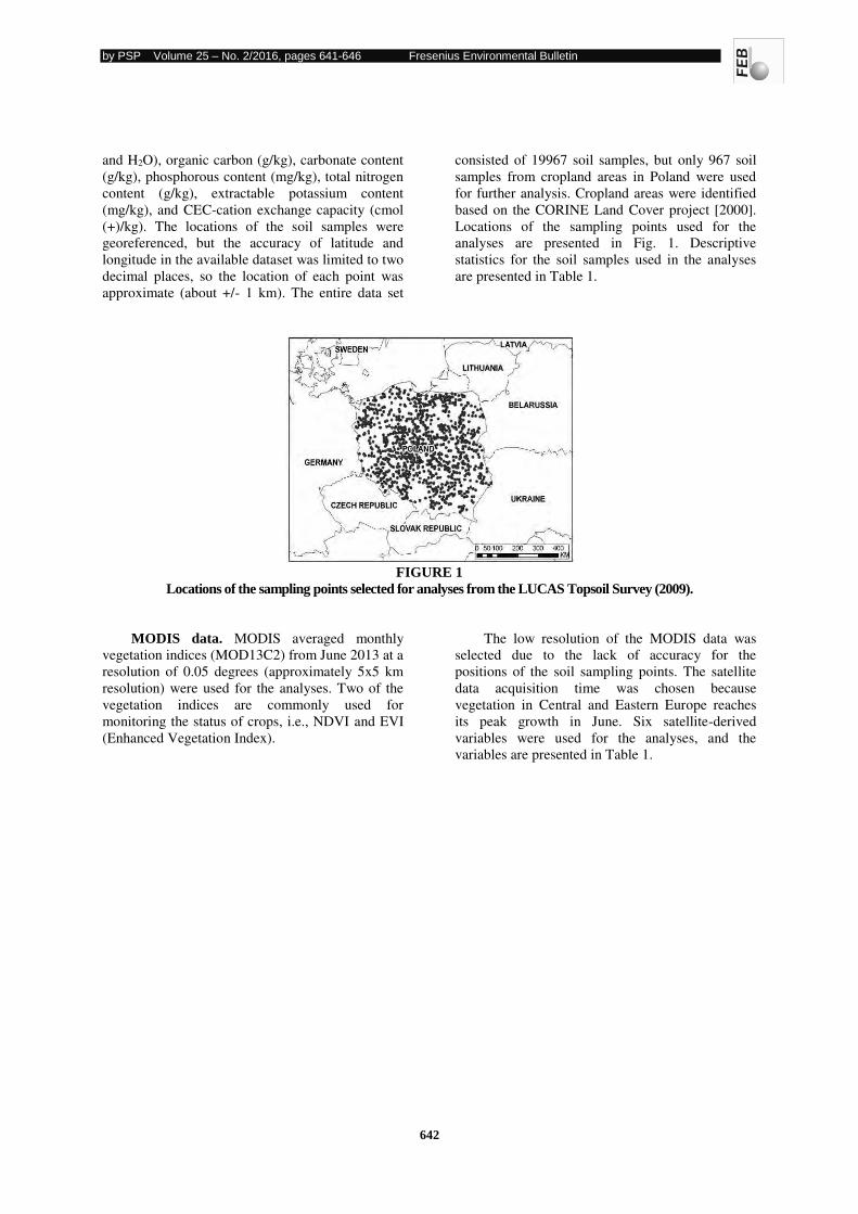
by PSP Volume 25 – No. 2/2016, pages 641-646 Fresenius Environmental Bulletin
642
and H2O), organic carbon (g/kg), carbonate content
(g/kg), phosphorous content (mg/kg), total nitrogen
content (g/kg), extractable potassium content
(mg/kg), and CEC-cation exchange capacity (cmol
(+)/kg). The locations of the soil samples were
georeferenced, but the accuracy of latitude and
longitude in the available dataset was limited to two
decimal places, so the location of each point was
approximate (about +/- 1 km). The entire data set
consisted of 19967 soil samples, but only 967 soil
samples from cropland areas in Poland were used
for further analysis. Cropland areas were identified
based on the CORINE Land Cover project [2000].
Locations of the sampling points used for the
analyses are presented in Fig. 1. Descriptive
statistics for the soil samples used in the analyses
are presented in Table 1.
FIGURE 1
Locations of the sampling points selected for analyses from the LUCAS Topsoil Survey (2009).
MODIS data. MODIS averaged monthly
vegetation indices (MOD13C2) from June 2013 at a
resolution of 0.05 degrees (approximately 5x5 km
resolution) were used for the analyses. Two of the
vegetation indices are commonly used for
monitoring the status of crops, i.e., NDVI and EVI
(Enhanced Vegetation Index).
The low resolution of the MODIS data was
selected due to the lack of accuracy for the
positions of the soil sampling points. The satellite
data acquisition time was chosen because
vegetation in Central and Eastern Europe reaches
its peak growth in June. Six satellite-derived
variables were used for the analyses, and the
variables are presented in Table 1.
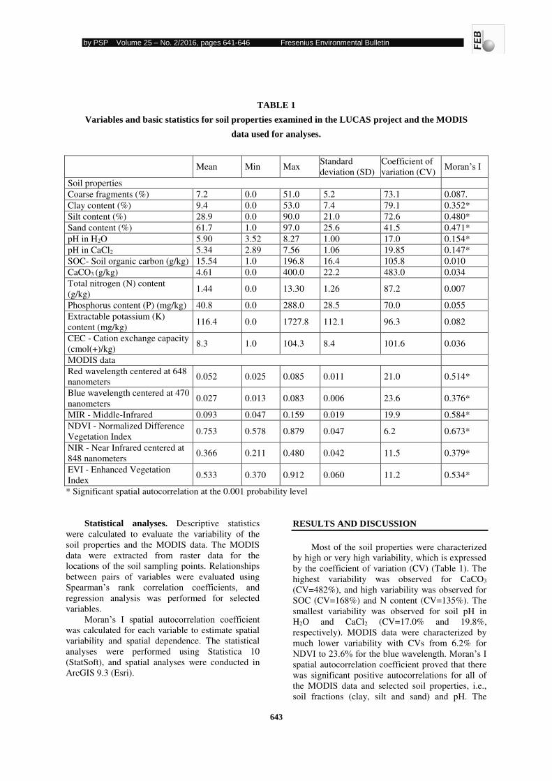
by PSP Volume 25 – No. 2/2016, pages 641-646 Fresenius Environmental Bulletin
643
TABLE 1
Variables and basic statistics for soil properties examined in the LUCAS project and the MODIS
data used for analyses.
Mean Min Max Standard
deviation (SD)
Coefficient of
variation (CV) Moran’s I
Soil properties
Coarse fragments (%) 7.2 0.0 51.0 5.2 73.1 0.087.
Clay content (%) 9.4 0.0 53.0 7.4 79.1 0.352*
Silt content (%) 28.9 0.0 90.0 21.0 72.6 0.480*
Sand content (%) 61.7 1.0 97.0 25.6 41.5 0.471*
pH in H2O 5.90 3.52 8.27 1.00 17.0 0.154*
pH in CaCl2 5.34 2.89 7.56 1.06 19.85 0.147*
SOC- Soil organic carbon (g/kg) 15.54 1.0 196.8 16.4 105.8 0.010
CaCO3 (g/kg) 4.61 0.0 400.0 22.2 483.0 0.034
Total nitrogen (N) content
(g/kg) 1.44 0.0 13.30 1.26 87.2 0.007
Phosphorus content (P) (mg/kg) 40.8 0.0 288.0 28.5 70.0 0.055
Extractable potassium (K)
content (mg/kg) 116.4 0.0 1727.8 112.1 96.3 0.082
CEC - Cation exchange capacity
(cmol(+)/kg) 8.3 1.0 104.3 8.4 101.6 0.036
MODIS data
Red wavelength centered at 648
nanometers 0.052 0.025 0.085 0.011 21.0 0.514*
Blue wavelength centered at 470
nanometers 0.027 0.013 0.083 0.006 23.6 0.376*
MIR - Middle-Infrared 0.093 0.047 0.159 0.019 19.9 0.584*
NDVI - Normalized Difference
Vegetation Index 0.753 0.578 0.879 0.047 6.2 0.673*
NIR - Near Infrared centered at
848 nanometers 0.366 0.211 0.480 0.042 11.5 0.379*
EVI - Enhanced Vegetation
Index 0.533 0.370 0.912 0.060 11.2 0.534*
* Significant spatial autocorrelation at the 0.001 probability level
Statistical analyses. Descriptive statistics
were calculated to evaluate the variability of the
soil properties and the MODIS data. The MODIS
data were extracted from raster data for the
locations of the soil sampling points. Relationships
between pairs of variables were evaluated using
Spearman’s rank correlation coefficients, and regression analysis was performed for selected
variables.
Moran’s I spatial autocorrelation coefficient was calculated for each variable to estimate spatial
variability and spatial dependence. The statistical
analyses were performed using Statistica 10
(StatSoft), and spatial analyses were conducted in
ArcGIS 9.3 (Esri).
RESULTS AND DISCUSSION
Most of the soil properties were characterized
by high or very high variability, which is expressed
by the coefficient of variation (CV) (Table 1). The
highest variability was observed for CaCO3
(CV=482%), and high variability was observed for
SOC (CV=168%) and N content (CV=135%). The
smallest variability was observed for soil pH in
H2O and CaCl2 (CV=17.0% and 19.8%,
respectively). MODIS data were characterized by
much lower variability with CVs from 6.2% for
NDVI to 23.6% for the blue wavelength. Moran’s I spatial autocorrelation coefficient proved that there
was significant positive autocorrelations for all of
the MODIS data and selected soil properties, i.e.,
soil fractions (clay, silt and sand) and pH. The
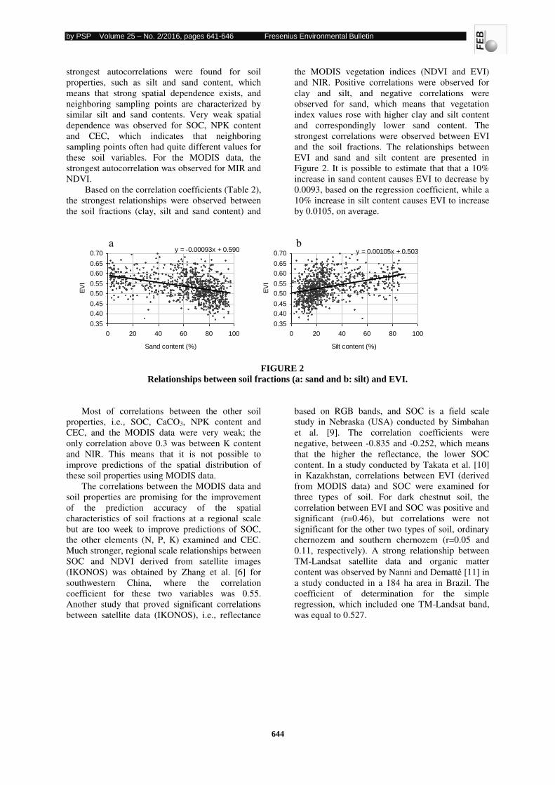
by PSP Volume 25 – No. 2/2016, pages 641-646 Fresenius Environmental Bulletin
644
strongest autocorrelations were found for soil
properties, such as silt and sand content, which
means that strong spatial dependence exists, and
neighboring sampling points are characterized by
similar silt and sand contents. Very weak spatial
dependence was observed for SOC, NPK content
and CEC, which indicates that neighboring
sampling points often had quite different values for
these soil variables. For the MODIS data, the
strongest autocorrelation was observed for MIR and
NDVI.
Based on the correlation coefficients (Table 2),
the strongest relationships were observed between
the soil fractions (clay, silt and sand content) and
the MODIS vegetation indices (NDVI and EVI)
and NIR. Positive correlations were observed for
clay and silt, and negative correlations were
observed for sand, which means that vegetation
index values rose with higher clay and silt content
and correspondingly lower sand content. The
strongest correlations were observed between EVI
and the soil fractions. The relationships between
EVI and sand and silt content are presented in
Figure 2. It is possible to estimate that that a 10%
increase in sand content causes EVI to decrease by
0.0093, based on the regression coefficient, while a
10% increase in silt content causes EVI to increase
by 0.0105, on average.
FIGURE 2
Relationships between soil fractions (a: sand and b: silt) and EVI.
Most of correlations between the other soil
properties, i.e., SOC, CaCO3, NPK content and
CEC, and the MODIS data were very weak; the
only correlation above 0.3 was between K content
and NIR. This means that it is not possible to
improve predictions of the spatial distribution of
these soil properties using MODIS data.
The correlations between the MODIS data and
soil properties are promising for the improvement
of the prediction accuracy of the spatial
characteristics of soil fractions at a regional scale
but are too week to improve predictions of SOC,
the other elements (N, P, K) examined and CEC.
Much stronger, regional scale relationships between
SOC and NDVI derived from satellite images
(IKONOS) was obtained by Zhang et al. [6] for
southwestern China, where the correlation
coefficient for these two variables was 0.55.
Another study that proved significant correlations
between satellite data (IKONOS), i.e., reflectance
based on RGB bands, and SOC is a field scale
study in Nebraska (USA) conducted by Simbahan
et al. [9]. The correlation coefficients were
negative, between -0.835 and -0.252, which means
that the higher the reflectance, the lower SOC
content. In a study conducted by Takata et al. [10]
in Kazakhstan, correlations between EVI (derived
from MODIS data) and SOC were examined for
three types of soil. For dark chestnut soil, the
correlation between EVI and SOC was positive and
significant (r=0.46), but correlations were not
significant for the other two types of soil, ordinary
chernozem and southern chernozem (r=0.05 and
0.11, respectively). A strong relationship between
TM-Landsat satellite data and organic matter
content was observed by Nanni and Demattê [11] in
a study conducted in a 184 ha area in Brazil. The
coefficient of determination for the simple
regression, which included one TM-Landsat band,
was equal to 0.527.
y = -0.00093x + 0.590
0.35
0.40
0.45
0.50
0.55
0.60
0.65
0.70
0 20 40 60 80 100
Sand content (%)
EV
I
y = 0.00105x + 0.503
0.35
0.40
0.45
0.50
0.55
0.60
0.65
0.70
0 20 40 60 80 100
Silt content (%)
EV
I
b a
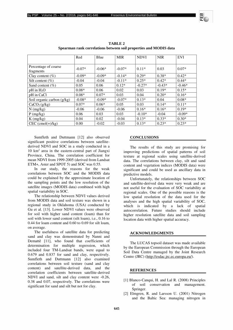
by PSP Volume 25 – No. 2/2016, pages 641-646 Fresenius Environmental Bulletin
645
TABLE 2
Spearman rank correlations between soil properties and MODIS data
Red Blue MIR NDVI NIR EVI
Percentage of coarse
fragments -0.07* -0.06* -0.07* 0.11* 0.03 0.07*
Clay content (%) -0.09* -0.09* -0.14* 0.29* 0.38* 0.42*
Silt content (%) -0.04 -0.04 -0.11* 0.25* 0.42* 0.44*
Sand content (%) 0.05 0.06 0.12* -0.27* -0.43* -0.46*
pH in H2O 0.08* 0.06 0.02 0.03 0.19* 0.15*
pH in CaCl 0.08* 0.07* 0.03 0.04 0.20* 0.16*
Soil organic carbon (g/kg) -0.08* -0.09* -0.07* 0.13* 0.04 0.08*
CaCO3 (g/kg) 0.07* 0.06* 0.05 0.03 0.14* 0.11*
N (mg/kg) -0.06 -0.06 -0.06 0.16* 0.16* 0.19*
P (mg/kg) 0.06 0.03 0.03 -0.10* -0.04 -0.09*
K (mg/kg) 0.04 0.02 -0.04 0.13* 0.33* 0.30*
CEC (cmol(+)/kg) 0.00 -0.02 -0.03 0.13* 0.23* 0.23*
Sumfleth and Duttmann [12] also observed
significant positive correlations between satellite-
derived NDVI and SOC in a study conducted in a
10 km2 area in the eastern-central part of Jiangxi
Province, China. The correlation coefficient for
mean NDVI from 1999-2005 (derived from Landsat
ETM+, Aster and SPOT 5) and SOC was 0.55.
In our study, the reasons for the weak
correlations between SOC and the MODIS data
could be explained by the approximate location of
the sampling points and the low resolution of the
satellite images (MODIS data) combined with high
spatial variability in SOC.
The relationship between NDVI values derived
from MODIS data and soil texture was shown in a
regional study in Oklahoma (USA) conducted by
Gu et al. [13]. Lower NDVI values were observed
for soil with higher sand content (loam) than for
soil with lower sand content (silt loam), i.e., 0.16 to
0.44 for loam content and 0.60 to 0.69 for silt loam,
on average.
The usefulness of satellite data for predicting
sand and clay was demonstrated by Nanni and
Demattê [11], who found that coefficients of
determination for multiple regression, which
included four TM-Landsat bands, were equal to
0.679 and 0.837 for sand and clay, respectively.
Sumfleth and Duttmann [12] also examined
correlations between soil texture (sand and clay
content) and satellite-derived data, and the
correlation coefficients between satellite-derived
NDVI and sand, silt and clay content were -0.26,
0.38 and 0.07, respectively. The correlations were
significant for sand and silt but not for clay.
CONCLUSIONS
The results of this study are promising for
improving predictions of spatial patterns of soil
texture at regional scales using satellite-derived
data. The correlations between clay, silt and sand
content and vegetation indices (MODIS data) were
significant and could be used as ancillary data in
predictive models.
Unfortunately, the relationships between SOC
and satellite-derived data were very weak and are
not useful for the evaluation of SOC variability at
regional scales. One of the possible reasons is the
low spatial resolution of the data used for the
analyses and the high spatial variability of SOC,
which is indicated by a lack of spatial
autocorrelation. Future studies should include
higher resolution satellite data and soil sampling
location data with higher spatial accuracy.
ACKNOWLEDGMENTS
The LUCAS topsoil dataset was made available
by the European Commission through the European
Soil Data Centre managed by the Joint Research
Centre (JRC) (http://esdac.jrc.ec.europa.eu/).
REFERENCES
[1] Blanco-Canqui, H. and Lal R. (2008) Principles
of soil conservation and management.
Springer.
[2] Elmgren, R. and Larsson U. (2001) Nitrogen
and the Baltic Sea: managing nitrogen in
by PSP Volume 25 – No. 2/2016, pages 641-646 Fresenius Environmental Bulletin
646
relation to phosphorus. Sci. World J., 1, 371-
377.
[3] Poggio, L., Gimona A. and Brewer M. J. (2013)
Regional scale mapping of soil properties and
their uncertainty with a large number of
satellite-derived covariates. Geoderma, 209, 1-
14.
[4] Dobos, E., Seres, A., Vadnai, P., Michéli, E.,
Fuchs, M., Láng, V., Bertoti, R.D. and
Kovács, K. (2013) Soil parent material
delineation using MODIS and SRTM data.
Hungarian Geographical Bulletin, 62, 133-
156.
[5] Kumar, S., Lal, R. and Liu D. (2012) A
geographically weighted regression kriging
approach for mapping soil organic carbon
stock. Geoderma, 189, 627-634.
[6] Zhang, W., Wang, K., Chen, H., He, X. and
Zhang J. (2012) Ancillary information
improves kriging on soil organic carbon data
for a typical karst peak cluster depression
landscape. J. Sci. Food Agr., 92, 1094-1102.
[7] Liao, K., Xu, S., Wu, J. and Zhu Q. (2013)
Spatial estimation of surface soil texture using
remote sensing data. Soil Sci. Plant Nutr., 59,
488-500.
[8] Carre, F., Rusco, E., Tóth, G., Jones, A., Gardi,
C. and Stolbovoy V. (2013) 2. Soil sampling
methodology. In: Tóth G., Jones A. and
Montanarella L.(eds.) LUCAS Topsoil Survey
methodology, data and results, Joint Research
Centre, Report EUR 26102.
[9] Simbahan, G. C., Dobermann, A., Goovaerts,
P., Ping, J. and Haddix M. L. (2006) Fine-
resolution mapping of soil organic carbon
based on multivariate secondary data.
Geoderma, 132, 471-489.
[10] Takata, Y., Funakawa, S., Akshalov, K.,
Ishida, N. and Kosaki T. (2007) Spatial
prediction of soil organic matter in northern
Kazakhstan based on topographic and
vegetation information. Soil Sci. Plant Nutr.,
53, 289-299.
[11] Nanni, M. R. and Demattê J.A.M. (2006)
Spectral reflectance methodology in
comparison to traditional soil analysis. Soil
Sci. Soc. Am. J., 70, 393-407.
[12] Sumfleth, K. and Duttmann R. (2008)
Prediction of soil property distribution in
paddy soil landscapes using terrain data and
satellite information as indicators. Ecol. Indic.,
8, 485-501.
[13] Gu, Y., Hunt, E., Wardlow, B., Basara, J. B.,
Brown, J. F. and Verdin J. P. (2008)
Evaluation of MODIS NDVI and NDWI for
vegetation drought monitoring using
Oklahoma Mesonet soil moisture data.
Geophys. Res. Lett., 35, L22401.
Received: 08.10.2015
Accepted: 27.01.2016
CORRESPONDING AUTHOR
Dariusz Gozdowski
Department of Experimental Design and
Bioinformatics
Warsaw University of Life Sciences
Nowoursynowska 159, 02-776 Warsaw – POLAND
e-mail: [email protected]
by PSP Volume 25 – No. 2/ 2016, pages 647-657 Fresenius Environmental Bulletin
647
EFFECTS OF ORGANIC FERTILIZER INPUT ON HEAVY
METAL CONTENT AND SPECIATION IN VEGETABLE AND
SOIL
Yaning Han1, Mengmeng Rui2, Yi Hao1, Yukiu Rui1,3, Xinlian Tang2, Liming Liu1, Weidong Cao4,5
1 College of Resources and Environmental Sciences, China Agricultural University, Beijing 100193, China
2 College of Agriculture, Guangxi University, Nanning 530005, China
3 Stockbridge School of Agriculture,University of Massachusetts, Amherst, MA 01003 USA
4 Key Laboratory of Plant Nutrition and Fertilizer, Ministry of Agriculture of the P.R. China/ Institute of Agricultural Resources and
Regional Planning, Chinese Academy of Agricultural Sciences, Beijing 100081, P.R. China
5 Qinghai Academy of Agricultural and Forestry, Qinghai University, Xining 810016, P.R. China
ABSTRACT
Long-term application of manure as organic
fertilizer results in high levels of heavy metals
accumulating in soil and vegetables. We studied the
effects of applying organic fertilizer to soil during
the cultivation process of Wuta-tsai (Brassica
campestris L. ssp. chinensis L. Makino var.
rosularis Tsen et Lee), and the speciation change of
zinc. Different levels of chicken manure were used
to look at the effect of heavy metal content and
speciation on Wuta-tsai and soil. Using synchrotron
radiation technology we determined the proportion
of each of the chemical forms of zinc in exposed
soils and plants quantitatively. The results show
that the optimum amount of chicken manure
fertilizer is 3.8 kg·m−2. This quantity increases
crop yield while reducing the accumulation of
heavy metals in Wuta-tsai.
KEYWORDS: Organic fertilizer, Wuta-tsai, heavy metals, speciation,
content
INTRODUCTION
Organic fertilizer contains abundant quantities
of organic matter and a variety of nutritional
elements. It is widely available, is derived from
multiple sources, and is nutrient-dense. It has been
shown that long-term application of manure affects
soil nutrient content, bacterial communities, and gas
emission rates [1]. Organic fertilizer can increase
soil pH and the cation exchange capacity, and
enhance nutrient levels in soils [2]. In the United
States, Western Europe, and in other developed
countries, where use of eco-agriculture and organic
agriculture techniques is increasing, organic manure
is becoming a primary source for fertilizing
organically grown vegetables. The Ministry of
Agriculture of the People’s Republic of China has set guidelines for zero growth in chemical fertilizer
use by 2020. Organic fertilizer instead of chemical
fertilizer was offered in the technology pathway,
meanwhile promote precision fertilization. This can
be accomplished with optimal utilization of
livestock and poultry.
Organic fertilizer is greatly important in
agriculture, but excessive use could have adverse
effects for the environment, soils, and crops. Kumar
et al. found that metals accumulated in plants and
soil in correlation with sewage sludge
concentrations [3-4]. Another studies also reported
that heavy metal contents in vegetables correlated
with heavy metal concentrations in soil [5-7]. Thus,
in organic cultivation, it is important to control
heavy metal content in organic fertilizer and the
amount of organic fertilizer applied. In the process
of large-scale livestock and poultry breeding, metal
trace element additives such as copper (Cu),
manganese (Mn), arsenic (As), and zinc (Zn), are
used to prevent animal diseases and promote the
growth and development of livestock and poultry.
Liu et al.’s research suggests that maximum concentrations of cadmium (Cd), chromium (Cr),
Cu, Zn, and As found in manures all exceeded
German and Italian standards, and soils exposed to
long-term chicken manure application accumulated
considerable amounts of metals [5]. An
investigation of 140 commercial organic fertilizer
with livestock and poultry manure, city garbage,
sewage sludge, industry and agricultural wastes,
weathered coal, and phosphate rock powder as the
main raw material, this research shows that the
content of Cd, mercury (Hg), lead (Pb), Cr and As
in commercial organic fertilizer were all over
weight by different degrees [8]. Excessive and
long-term use of fertilizers and livestock manure
that contain high levels of heavy metal leads to the
accumulation of heavy metals in soils [9]. In
manure-treated soils, levels of heavy metals were
significantly higher than the natural background
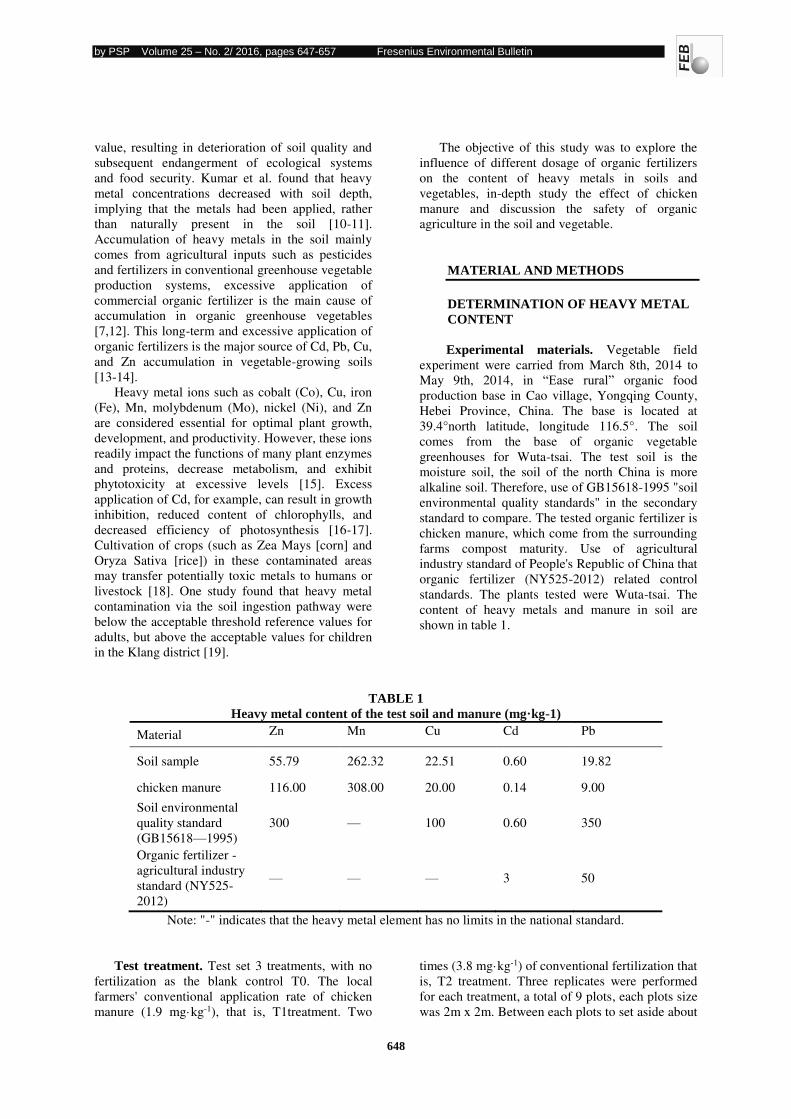
by PSP Volume 25 – No. 2/ 2016, pages 647-657 Fresenius Environmental Bulletin
648
value, resulting in deterioration of soil quality and
subsequent endangerment of ecological systems
and food security. Kumar et al. found that heavy
metal concentrations decreased with soil depth,
implying that the metals had been applied, rather
than naturally present in the soil [10-11].
Accumulation of heavy metals in the soil mainly
comes from agricultural inputs such as pesticides
and fertilizers in conventional greenhouse vegetable
production systems, excessive application of
commercial organic fertilizer is the main cause of
accumulation in organic greenhouse vegetables
[7,12]. This long-term and excessive application of
organic fertilizers is the major source of Cd, Pb, Cu,
and Zn accumulation in vegetable-growing soils
[13-14].
Heavy metal ions such as cobalt (Co), Cu, iron
(Fe), Mn, molybdenum (Mo), nickel (Ni), and Zn
are considered essential for optimal plant growth,
development, and productivity. However, these ions
readily impact the functions of many plant enzymes
and proteins, decrease metabolism, and exhibit
phytotoxicity at excessive levels [15]. Excess
application of Cd, for example, can result in growth
inhibition, reduced content of chlorophylls, and
decreased efficiency of photosynthesis [16-17].
Cultivation of crops (such as Zea Mays [corn] and
Oryza Sativa [rice]) in these contaminated areas
may transfer potentially toxic metals to humans or
livestock [18]. One study found that heavy metal
contamination via the soil ingestion pathway were
below the acceptable threshold reference values for
adults, but above the acceptable values for children
in the Klang district [19].
The objective of this study was to explore the
influence of different dosage of organic fertilizers
on the content of heavy metals in soils and
vegetables, in-depth study the effect of chicken
manure and discussion the safety of organic
agriculture in the soil and vegetable.
MATERIAL AND METHODS
DETERMINATION OF HEAVY METAL
CONTENT
Experimental materials. Vegetable field
experiment were carried from March 8th, 2014 to
May 9th, 2014, in “Ease rural” organic food
production base in Cao village, Yongqing County,
Hebei Province, China. The base is located at
39.4°north latitude, longitude 116.5°. The soil
comes from the base of organic vegetable
greenhouses for Wuta-tsai. The test soil is the
moisture soil, the soil of the north China is more
alkaline soil. Therefore, use of GB15618-1995 "soil
environmental quality standards" in the secondary
standard to compare. The tested organic fertilizer is
chicken manure, which come from the surrounding
farms compost maturity. Use of agricultural
industry standard of People's Republic of China that
organic fertilizer (NY525-2012) related control
standards. The plants tested were Wuta-tsai. The
content of heavy metals and manure in soil are
shown in table 1.
TABLE 1
Heavy metal content of the test soil and manure (mg·kg-1)
Material Zn
Mn
Cu
Cd
Pb
Soil sample 55.79 262.32 22.51 0.60 19.82
chicken manure 116.00 308.00 20.00 0.14 9.00
Soil environmental
quality standard
(GB15618—1995)
300 — 100 0.60 350
Organic fertilizer -
agricultural industry
standard (NY525-
2012)
— — — 3 50
Note: "-" indicates that the heavy metal element has no limits in the national standard.
Test treatment. Test set 3 treatments, with no
fertilization as the blank control T0. The local
farmers' conventional application rate of chicken
manure (1.9 mg·kg-1), that is, T1treatment. Two
times (3.8 mg·kg-1) of conventional fertilization that
is, T2 treatment. Three replicates were performed
for each treatment, a total of 9 plots, each plots size
was 2m x 2m. Between each plots to set aside about
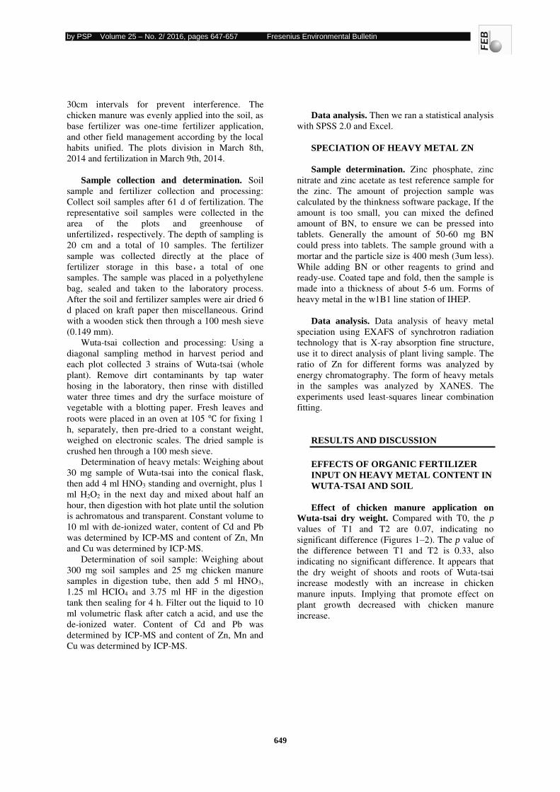
by PSP Volume 25 – No. 2/ 2016, pages 647-657 Fresenius Environmental Bulletin
649
30cm intervals for prevent interference. The
chicken manure was evenly applied into the soil, as
base fertilizer was one-time fertilizer application,
and other field management according by the local
habits unified. The plots division in March 8th,
2014 and fertilization in March 9th, 2014.
Sample collection and determination. Soil
sample and fertilizer collection and processing:
Collect soil samples after 61 d of fertilization. The
representative soil samples were collected in the
area of the plots and greenhouse of
unfertilized,respectively. The depth of sampling is
20 cm and a total of 10 samples. The fertilizer
sample was collected directly at the place of
fertilizer storage in this base,a total of one
samples. The sample was placed in a polyethylene
bag, sealed and taken to the laboratory process.
After the soil and fertilizer samples were air dried 6
d placed on kraft paper then miscellaneous. Grind
with a wooden stick then through a 100 mesh sieve
(0.149 mm).
Wuta-tsai collection and processing: Using a
diagonal sampling method in harvest period and
each plot collected 3 strains of Wuta-tsai (whole
plant). Remove dirt contaminants by tap water
hosing in the laboratory, then rinse with distilled
water three times and dry the surface moisture of
vegetable with a blotting paper. Fresh leaves and
roots were placed in an oven at 105 ℃ for fixing 1
h, separately, then pre-dried to a constant weight,
weighed on electronic scales. The dried sample is
crushed hen through a 100 mesh sieve.
Determination of heavy metals: Weighing about
30 mg sample of Wuta-tsai into the conical flask,
then add 4 ml HNO3 standing and overnight, plus 1
ml H2O2 in the next day and mixed about half an
hour, then digestion with hot plate until the solution
is achromatous and transparent. Constant volume to
10 ml with de-ionized water, content of Cd and Pb
was determined by ICP-MS and content of Zn, Mn
and Cu was determined by ICP-MS.
Determination of soil sample: Weighing about
300 mg soil samples and 25 mg chicken manure
samples in digestion tube, then add 5 ml HNO3,
1.25 ml HCIO4 and 3.75 ml HF in the digestion
tank then sealing for 4 h. Filter out the liquid to 10
ml volumetric flask after catch a acid, and use the
de-ionized water. Content of Cd and Pb was
determined by ICP-MS and content of Zn, Mn and
Cu was determined by ICP-MS.
Data analysis. Then we ran a statistical analysis
with SPSS 2.0 and Excel.
SPECIATION OF HEAVY METAL ZN
Sample determination. Zinc phosphate, zinc
nitrate and zinc acetate as test reference sample for
the zinc. The amount of projection sample was
calculated by the thinkness software package, If the
amount is too small, you can mixed the defined
amount of BN, to ensure we can be pressed into
tablets. Generally the amount of 50-60 mg BN
could press into tablets. The sample ground with a
mortar and the particle size is 400 mesh (3um less).
While adding BN or other reagents to grind and
ready-use. Coated tape and fold, then the sample is
made into a thickness of about 5-6 um. Forms of
heavy metal in the w1B1 line station of IHEP.
Data analysis. Data analysis of heavy metal
speciation using EXAFS of synchrotron radiation
technology that is X-ray absorption fine structure,
use it to direct analysis of plant living sample. The
ratio of Zn for different forms was analyzed by
energy chromatography. The form of heavy metals
in the samples was analyzed by XANES. The
experiments used least-squares linear combination
fitting.
RESULTS AND DISCUSSION
EFFECTS OF ORGANIC FERTILIZER
INPUT ON HEAVY METAL CONTENT IN
WUTA-TSAI AND SOIL
Effect of chicken manure application on Wuta-tsai dry weight. Compared with T0, the p
values of T1 and T2 are 0.07, indicating no
significant difference (Figures 1–2). The p value of
the difference between T1 and T2 is 0.33, also
indicating no significant difference. It appears that
the dry weight of shoots and roots of Wuta-tsai
increase modestly with an increase in chicken
manure inputs. Implying that promote effect on
plant growth decreased with chicken manure
increase.
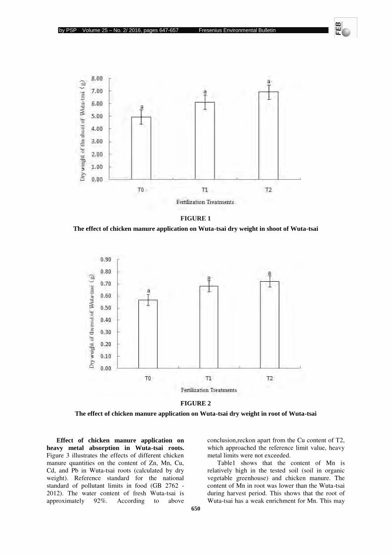
by PSP Volume 25 – No. 2/ 2016, pages 647-657 Fresenius Environmental Bulletin
650
FIGURE 1
The effect of chicken manure application on Wuta-tsai dry weight in shoot of Wuta-tsai
FIGURE 2
The effect of chicken manure application on Wuta-tsai dry weight in root of Wuta-tsai
Effect of chicken manure application on
heavy metal absorption in Wuta-tsai roots.
Figure 3 illustrates the effects of different chicken
manure quantities on the content of Zn, Mn, Cu,
Cd, and Pb in Wuta-tsai roots (calculated by dry
weight). Reference standard for the national
standard of pollutant limits in food (GB 2762 -
2012). The water content of fresh Wuta-tsai is
approximately 92%. According to above
conclusion,reckon apart from the Cu content of T2,
which approached the reference limit value, heavy
metal limits were not exceeded.
Table1 shows that the content of Mn is
relatively high in the tested soil (soil in organic
vegetable greenhouse) and chicken manure. The
content of Mn in root was lower than the Wuta-tsai
during harvest period. This shows that the root of
Wuta-tsai has a weak enrichment for Mn. This may
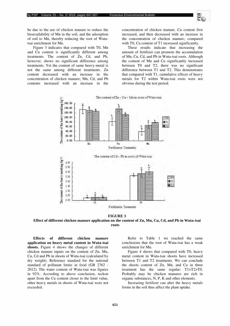
by PSP Volume 25 – No. 2/ 2016, pages 647-657 Fresenius Environmental Bulletin
651
be due to the use of chicken manure to reduce the
bioavailability of Mn in the soil, and the adsorption
of soil to Mn, thereby reducing the root of Wuta-
tsai enrichment for Mn.
Figure 3 indicates that compared with T0, Mn
and Cu content is significantly different among
treatments. The content of Zn, Cd, and Pb,
however, shows no significant difference among
treatments. Yet the content of same heavy-metal is
not the same among different treatments. Zn
content decreased with an increase in the
concentration of chicken manure; Mn, Cd, and Pb
contents increased with an increase in the
concentration of chicken manure. Cu content first
increased, and then decreased with an increase in
the concentration of chicken manure; compared
with T0, Cu content of T1 increased significantly.
These results indicate that increasing the
amount of fertilizer can promote the accumulation
of Mn, Cu, Cd, and Pb in Wuta-tsai roots. Although
the content of Mn and Cu significantly increased
between T0 and T2, there was no significant
difference between T1 and T2. This demonstrates
that compared with T1, cumulative effects of heavy
metals for T2 within Wuta-tsai roots were not
obvious during the test period.
FIGURE 3
Effect of different chicken manure application on the content of Zn, Mn, Cu, Cd, and Pb in Wuta-tsai
roots
Effects of different chicken manure
application on heavy metal content in Wuta-tsai
shoots. Figure 4 shows the changes of different
chicken manure inputs on the content of Zn, Mn,
Cu, Cd and Pb in shoots of Wuta-tsai (calculated by
dry weight). Reference standard for the national
standard of pollutant limits in food (GB 2762 -
2012). The water content of Wuta-tsai was figures
in 92%. According to above conclusion, reckon
apart from the Cu content closer to the limit value,
other heavy metals in shoots of Wuta-tsai were not
exceeded.
Refer to Table 1 we reached the same
conclusions that the root of Wuta-tsai has a weak
enrichment for Mn.
Figure 4 shows that compared with T0, heavy
metal content in Wuta-tsai shoots have increased
between T1 and T2 treatments. We can conclude
the shoots content of Zn, Mn, and Cu in three
treatment has the same regular: T1>T2>T0.
Probably may be chicken manures are rich in
organic substances, N, P, K and other elements.
Increasing fertilizer can alter the heavy metals
forms in the soil thus affect the plant uptake.
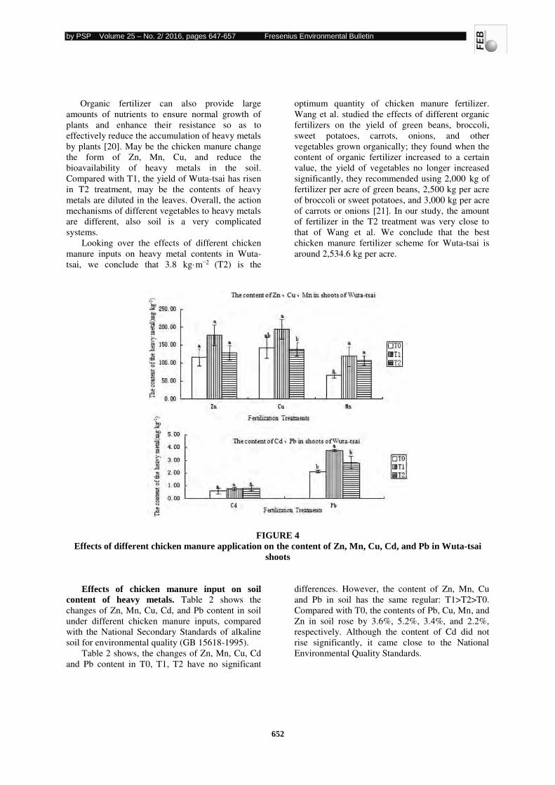
by PSP Volume 25 – No. 2/ 2016, pages 647-657 Fresenius Environmental Bulletin
652
Organic fertilizer can also provide large
amounts of nutrients to ensure normal growth of
plants and enhance their resistance so as to
effectively reduce the accumulation of heavy metals
by plants [20]. May be the chicken manure change
the form of Zn, Mn, Cu, and reduce the
bioavailability of heavy metals in the soil.
Compared with T1, the yield of Wuta-tsai has risen
in T2 treatment, may be the contents of heavy
metals are diluted in the leaves. Overall, the action
mechanisms of different vegetables to heavy metals
are different, also soil is a very complicated
systems.
Looking over the effects of different chicken
manure inputs on heavy metal contents in Wuta-
tsai, we conclude that 3.8 kg·m−2 (T2) is the
optimum quantity of chicken manure fertilizer.
Wang et al. studied the effects of different organic
fertilizers on the yield of green beans, broccoli,
sweet potatoes, carrots, onions, and other
vegetables grown organically; they found when the
content of organic fertilizer increased to a certain
value, the yield of vegetables no longer increased
significantly, they recommended using 2,000 kg of
fertilizer per acre of green beans, 2,500 kg per acre
of broccoli or sweet potatoes, and 3,000 kg per acre
of carrots or onions [21]. In our study, the amount
of fertilizer in the T2 treatment was very close to
that of Wang et al. We conclude that the best
chicken manure fertilizer scheme for Wuta-tsai is
around 2,534.6 kg per acre.
FIGURE 4
Effects of different chicken manure application on the content of Zn, Mn, Cu, Cd, and Pb in Wuta-tsai
shoots
Effects of chicken manure input on soil
content of heavy metals. Table 2 shows the
changes of Zn, Mn, Cu, Cd, and Pb content in soil
under different chicken manure inputs, compared
with the National Secondary Standards of alkaline
soil for environmental quality (GB 15618-1995).
Table 2 shows, the changes of Zn, Mn, Cu, Cd
and Pb content in T0, T1, T2 have no significant
differences. However, the content of Zn, Mn, Cu
and Pb in soil has the same regular: T1>T2>T0.
Compared with T0, the contents of Pb, Cu, Mn, and
Zn in soil rose by 3.6%, 5.2%, 3.4%, and 2.2%,
respectively. Although the content of Cd did not
rise significantly, it came close to the National
Environmental Quality Standards.
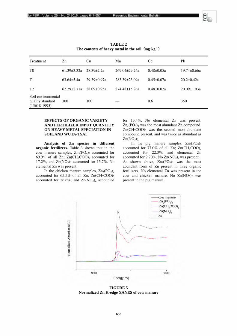
by PSP Volume 25 – No. 2/ 2016, pages 647-657 Fresenius Environmental Bulletin
653
TABLE 2
The contents of heavy metal in the soil mg·kg-1
Treatment Zn Cu Mn Cd Pb
T0 61.39±3.32a 28.39±2.2a 269.04±29.24a 0.48±0.05a 19.74±0.66a
T1 63.64±5.4a 29.39±0.97a 283.39±23.09a 0.45±0.07a 20.2±0.42a
T2 62.29±2.71a 28.09±0.95a 274.48±15.26a 0.48±0.02a 20.09±1.93a
Soil environmental
quality standard
(15618-1995)
300 100 — 0.6 350
EFFECTS OF ORGANIC VARIETY
AND FERTILIZER INPUT QUANTITY
ON HEAVY METAL SPECIATION IN
SOIL AND WUTA-TSAI
Analysis of Zn species in different
organic fertilizers. Table 3 shows that in the
cow manure samples, Zn3(PO4)2 accounted for
69.9% of all Zn; Zn(CH3COO)2 accounted for
17.2%, and Zn(NO3)2 accounted for 15.7%. No
elemental Zn was present.
In the chicken manure samples, Zn3(PO4)2
accounted for 65.5% of all Zn; Zn(CH3COO)2
accounted for 26.6%, and Zn(NO3)2 accounted
for 13.4%. No elemental Zn was present.
Zn3(PO4)2 was the most abundant Zn compound,
Zn(CH3COO)2 was the second most-abundant
compound present, and was twice as abundant as
Zn(NO3)2.
In the pig manure samples, Zn3(PO4)2
accounted for 77.0% of all Zn; Zn(CH3COO)2
accounted for 22.3%, and elemental Zn
accounted for 2.70%. No Zn(NO3)2 was present.
As shown above, Zn3(PO4)2 was the most
abundant form of Zn present in three organic
fertilizers. No elemental Zn was present in the
cow and chicken manure. No Zn(NO3)2 was
present in the pig manure.
FIGURE 5
Normalized Zn K-edge XANES of cow manure
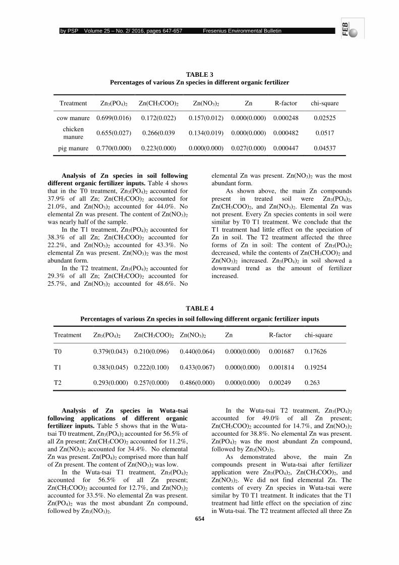
by PSP Volume 25 – No. 2/ 2016, pages 647-657 Fresenius Environmental Bulletin
654
TABLE 3
Percentages of various Zn species in different organic fertilizer
Analysis of Zn species in soil following different organic fertilizer inputs. Table 4 shows
that in the T0 treatment, Zn3(PO4)2 accounted for
37.9% of all Zn; Zn(CH3COO)2 accounted for
21.0%, and Zn(NO3)2 accounted for 44.0%. No
elemental Zn was present. The content of Zn(NO3)2
was nearly half of the sample.
In the T1 treatment, Zn3(PO4)2 accounted for
38.3% of all Zn; Zn(CH3COO)2 accounted for
22.2%, and Zn(NO3)2 accounted for 43.3%. No
elemental Zn was present. Zn(NO3)2 was the most
abundant form.
In the T2 treatment, Zn3(PO4)2 accounted for
29.3% of all Zn; Zn(CH3COO)2 accounted for
25.7%, and Zn(NO3)2 accounted for 48.6%. No
elemental Zn was present. Zn(NO3)2 was the most
abundant form.
As shown above, the main Zn compounds
present in treated soil were Zn3(PO4)2,
Zn(CH3COO)2, and Zn(NO3)2. Elemental Zn was
not present. Every Zn species contents in soil were
similar by T0 T1 treatment. We conclude that the
T1 treatment had little effect on the speciation of
Zn in soil. The T2 treatment affected the three
forms of Zn in soil: The content of Zn3(PO4)2
decreased, while the contents of Zn(CH3COO)2 and
Zn(NO3)2 increased. Zn3(PO4)2 in soil showed a
downward trend as the amount of fertilizer
increased.
TABLE 4
Percentages of various Zn species in soil following different organic fertilizer inputs
Analysis of Zn species in Wuta-tsai
following applications of different organic
fertilizer inputs. Table 5 shows that in the Wuta-
tsai T0 treatment, Zn3(PO4)2 accounted for 56.5% of
all Zn present; Zn(CH3COO)2 accounted for 11.2%,
and Zn(NO3)2 accounted for 34.4%. No elemental
Zn was present. Zn(PO4)2 comprised more than half
of Zn present. The content of Zn(NO3)2 was low.
In the Wuta-tsai T1 treatment, Zn3(PO4)2
accounted for 56.5% of all Zn present;
Zn(CH3COO)2 accounted for 12.7%, and Zn(NO3)2
accounted for 33.5%. No elemental Zn was present.
Zn(PO4)2 was the most abundant Zn compound,
followed by Zn3(NO3)2.
In the Wuta-tsai T2 treatment, Zn3(PO4)2
accounted for 49.0% of all Zn present;
Zn(CH3COO)2 accounted for 14.7%, and Zn(NO3)2
accounted for 38.8%. No elemental Zn was present.
Zn(PO4)2 was the most abundant Zn compound,
followed by Zn3(NO3)2.
As demonstrated above, the main Zn
compounds present in Wuta-tsai after fertilizer
application were Zn3(PO4)2, Zn(CH3COO)2, and
Zn(NO3)2. We did not find elemental Zn. The
contents of every Zn species in Wuta-tsai were
similar by T0 T1 treatment. It indicates that the T1
treatment had little effect on the speciation of zinc
in Wuta-tsai. The T2 treatment affected all three Zn
Treatment Zn3(PO4)2 Zn(CH3COO)2 Zn(NO3)2 Zn R-factor chi-square
cow manure 0.699(0.016) 0.172(0.022) 0.157(0.012) 0.000(0.000) 0.000248 0.02525
chicken
manure 0.655(0.027) 0.266(0.039 0.134(0.019) 0.000(0.000) 0.000482 0.0517
pig manure 0.770(0.000) 0.223(0.000) 0.000(0.000) 0.027(0.000) 0.000447 0.04537
Treatment Zn3(PO4)2 Zn(CH3COO)2 Zn(NO3)2 Zn R-factor chi-square
T0 0.379(0.043) 0.210(0.096) 0.440(0.064) 0.000(0.000) 0.001687 0.17626
T1 0.383(0.045) 0.222(0.100) 0.433(0.067) 0.000(0.000) 0.001814 0.19254
T2 0.293(0.000) 0.257(0.000) 0.486(0.000) 0.000(0.000) 0.00249 0.263
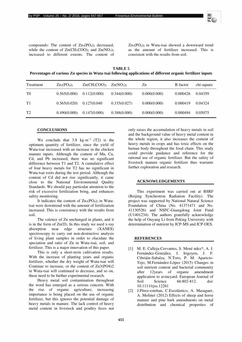
by PSP Volume 25 – No. 2/ 2016, pages 647-657 Fresenius Environmental Bulletin
655
compounds: The content of Zn3(PO4)2 decreased,
while the content of Zn(CH3COO)2 and Zn(NO3)2
increased to different extents. The content of
Zn3(PO4)2 in Wuta-tsai showed a downward trend
as the amount of fertilizer increased. This is
consistent with the results from soil.
TABLE 5
Percentages of various Zn species in Wuta-tsai following applications of different organic fertilizer inputs
Treatment Zn3(PO4)2 Zn(CH3COO)2 Zn(NO3)2 Zn R-factor chi-square
T0 0.565(0.000) 0.112(0.000) 0.344(0.000) 0.000(0.000) 0.000426 0.04359
T1 0.565(0.020) 0.127(0.040 0.335(0.027) 0.000(0.000) 0.000419 0.04324
T2 0.490(0.000) 0.147(0.000) 0.388(0.000) 0.000(0.000) 0.000494 0.05075
CONCLUSIONS
We conclude that 3.8 kg·m−2 (T2) is the
optimum quantity of fertilizer, since the yield of
Wuta-tsai increased with an increase in the chicken
manure inputs. Although the content of Mn, Cu,
Cd, and Pb increased, there was no significant
difference between T1 and T2. A cumulative effect
of four heavy metals for T2 has no significant in
Wuta-tsai roots during the test period. Although the
content of Cd did not rise significantly, it came
close to the National Environmental Quality
Standards. We should pay particular attention to the
risk of excessive fertilization bring, and enhances
safety monitoring.
It indicates the content of Zn3(PO4)2 in Wuta-
tsai were downtrend with the amount of fertilization
increased. This is consistency with the results from
soil.
The valence of Zn unchanged in plants, and it
is in the form of Zn(П). In this study we used x-ray
absorption near edge structure (XANES)
spectroscopy to carry out non-destructive analysis
of living plant samples in order to elucidate the
speciation and ratio of Zn in Wuta-tsai, soil, and
fertilizer. This is a major innovation of this paper.
This is only a short-term cultivation results.
With the increase of planting years and organic
fertilizer, whether the dry weight of Wuta-tsai will
Continue to increase, or the content of Zn3(PO4)2
in Wuta-tsai will continued to decrease, and so on,
these need to be further experimental research.
Heavy metal soil contamination throughout
the word has emerged as a serious concern. With
the rise of organic agriculture, increasing
importance is being placed on the use of organic
fertilizer, but this ignores the potential damage of
heavy metals in manure. The lack control of heavy
metal content in livestock and poultry feces not
only raises the accumulation of heavy metals in soil
and the background value of heavy metal content in
the whole region, it also increases the content of
heavy metals in crops and has toxic effects on the
human body throughout the food chain. This study
could provide guidance and reference for the
rational use of organic fertilizer. But the safety of
livestock manure organic fertilizer thus warrants
further exploration and research.
ACKNOWLEDGEMENTS
This experiment was carried out at BSRF
(Beijing Synchrotron Radiation Facility). The
project was supported by National Natural Science
Foundation of China (No. 41371471 and No.
41130526) and NSFC-Guangdong Joint Fund
(U1401234). The authors gratefully acknowledge
the help of Ouyang Li from Peking University with
determination of nutrient by ICP-MS and ICP-OES.
REFERENCES
[1] M. E. Calleja-Cervantes, S. Mené ndez*, A. J.
Fernández-González, I. Irigoyen, J. F.
Cibriáin-Sabalza, N.Toro, P. M. Aparicio-
Tejo, M.Fernández-López (2015) Changes in
soil nutrient content and bacterial community
after 12years of organic amendment
application to avineyard. European Journal of
Soil Science 66:802-812. doi:
10.1111/ejss.12261
[2] J.Pérez-esteban, C.Escolástico, A. Masaguer,
A. Moliner (2012) Effects of sheep and horse
manure and pine bark amendments on metal
distribution and chemical properties of
by PSP Volume 25 – No. 2/ 2016, pages 647-657 Fresenius Environmental Bulletin
656
contaminated mine soils . European Journal of
Soil Science, 63, 733–742
[3] Kumar V, A. K. Chopra (2014) Accumulation
and translocation of metals in soil and
different parts of French Bean
(Phaseolusvulgaris L.) Amendedwith Sewage
Sludge. Bulletin of Environmental
Contamination and Toxicology, 92:103–108
[4] Shomar B, Kalavrouziotis K I, Koukoulakis P
H, Yahya A (2013) Soil pollution indices
under the effect of sludge. Water Air Soil
Pollution, 224–1436
[5] Liu Q, Sun X, Hu A Y, Zhang Y A, Cao Z H
(2014) Characteristics of toxic metal
accumulation in farmlandin relation to long-
term chicken manure application:A case study
in the Yangtze River Delta Region,
China.Bulletin of Environmental
Contamination and Toxicology, 92:279–284
[6] Chen Z F, Zhao Y, Gu L, Wang S F. Li Y L,
Dong F L (2014) Accumulation and
localization of cadmium in potato(Solanum
tuberosum) under different soil Cd
levels.Bulletin of Environmental
Contamination and Toxicology, 92:745–751
[7] Chen Y, Huang B, Hu W Y, Weindorf D C,
Liu X X, Yang L Q (2014) Accumulation and
ecological effects of soil heavy metalsin
conventional and organic greenhouse
vegetable production systems in Nanjing,
China. Environmental Earth Sciences,
71:3605–3616
[8] Zhong X L, Zhou S L, Zhao Q G (2006) Soil
contamination and its Eco-environmental
impacts in the urban-rural marginal area.
Soils), 38(2):122–129
[9] Bai L Y, Zeng X B, Su S M, Duan R, Wang Y
N, Gao X (2015) Heavy metal accumulation
and source analysis in greenhouse soils of
Wuwei District, Gansu Province, China.
Environmental Science and Pollution
Research, 22:5359-5369
[10] Kumar A, Maiti S K (2015) Assessment of
potentially toxic heavy metal contaminationin
agricultural fields, sediment, and water from
an abandoned chromite-asbestos mine waste
of Roro hill, Chaibasa, India. Environmental
Earth Sciences
[11] Szolnoki Z, Farsang A (2013) Evaluation of
metal mobility and bioaccessibility in soils of
urban vegetable gardens using sequential
extraction . Water Air Soil Pollution, 224–1737
[12] Wu L H, Pan X, Chen L K, Huang Y J, Teng
Y, Luo Y M, Christie P (2013) Occurrence
and distribution of heavy metals and
tetracyclines in agricultural soils after typical
land use change ineast China. Environmental
Science and Pollution Research, 20:8342–8354
[13] Hu W Y, Huang B, Shi X Z, Chen W P, Zhao
Y G, Jiao W T (2013) Accumulation and
health risk of heavy metals in a plot-scale
vegetable production system in a peri-urban
vegetable farm near Nanjing, China.
Ecotoxicology and Environmental Safety ,
303–309
[14] Yang LQ, Huang B, Hu W Y, Chen Y, Mao
M C (2013) Assessment and source
identification of trace metals in the soils of
greenhouse vegetable production in eastern
China. Ecotoxicology and Environmental
Safety, 204–209
[15] Anjum N A, Singh H P, Khan M I R, Masood
A, Per T S, Negi A, Batish D R, Khan N A,
Duarte A C, Pereira E, Ahmad I (2015) Too
much is bad-an appraisal of phytotoxicity of
elevated plant-beneficial heavy metal ions.
Environmental Science and Pollution
Research, 22:3361–3382
[16] Saifullah, Sarwar N, Bibi S,Ahmad M, Sik Ok
Y (2014) Effectiveness of zinc application to
minimize cadmium toxicity and accumulation
in wheat(Triticum aestivum L.). Environ Earth
Sciences, 71:1663–1672
[17] Mihaličová Malčovská S, Dučaiová Z, Maslaňáková I, Bačkor M (2014) Effect of silicon on growth, photosynthesis, oxidative
status and phenolic compounds of maize (Zea
mays L.) grown in cadmium excess. Water Air
Soil Pollution, 225–2056
[18] Kuma A, Maiti S K (2014) Translocation and
bioaccumulation of metals in Oryza sativaand
Zea mays growing in chromite-asbestos
contaminated agricultural fields, Jharkhand,
India.Bulletin of Environmental
Contamination and Toxicology, 93:434–441
[19] Nurul Syazani Yuswir, Sarva Mangala
Praveena, Ahmad Zaharin Aris, Sharifah
Norkhadijah Syed Ismail, Zailina Hashim
(2015) Health risk assessment of heavy metal
in urban surface soil(Klang District,
Malaysia). Bulletin of Environmental
Contamination and Toxicology, 95:80–89
[20] Du C Y, Zu Y Q, Li Y (2005) Effect of pH
and organic matter on the bioavailability Cd
and Zn in soil.Journal of Yunnan Agricultural
University, 20(4):539–543
[21] Wang W J, Zhu D Y, Wang H S (2010) Effect
of different amount of organic fertilizer in the
yield of organic vegetables. Northern
Horticulture. (17):29–30

by PSP Volume 25 – No. 2/ 2016, pages 647-657 Fresenius Environmental Bulletin
657
Received: 17.10.2015
Accepted: 27.12.2015
CORRESPONDING AUTHOR
Rui Yukui
College of Resources and Environmental Sciences,
China Agricultural University
Beijing 100193 – P.R. CHINA
e-mail: [email protected].
by PSP Volume 25 – No. 2/2016, pages 658-664 Fresenius Environmental Bulletin
658
SHORT TERM EFFECTS OF ZINC ON SOME SERA
BIOCHEMICAL PARAMETERS AND ON TISSUE
ACCUMULATION OF Clarias gariepinus
Mustafa Tuncsoya, Servet Durana, Burcu Yesilbudaka, Özcan Ayb, Bedii Cicikb, Cahit Erdema
aUniversity of Cukurova, Faculty of Science and Letters, Biology Department, 01330 Balcalı, Adana, Turkey
bMersin University, Faculty of Fisheries, Yenişehir Campus, Yenişehir, Mersin, Turkey
ABSTRACT
Effects of zinc on sera aspartate
aminotransferase (AST), alanine aminotransferase
(ALT) activities and glucose, total protein and
cholesterol levels together with liver, gill, kidney,
spleen and muscle accumulation of the metal were
studied after exposing Clarias gariepinus to 1.0 and
5.0 ppm Zn over 24, 48 and 96 hours.
Highest accumulation of Zn was in liver and
spleen tissues in fish exposed to 1.0 ppm and 5.0
ppm Zn respectively after 96 hours of exposure.
Sera AST and ALT activities, cholesterol,
total protein and glucose levels changed depending
on zinc concentration and exposure period. Sera
glucose levels increased with increasing exposure
periods at both concentrations of zinc. There was
also an increase in sera cholesterol and total protein
levels at the beginning of the experiment which
decreased with increasing exposure. The increase in
sera ALT and AST activities were higher in 5.0
ppm Zn compared with 1.0 ppm Zn depending on
exposure period.
KEYWORDS: Clarias gariepinus, Sera biochemical parameters,
Accumulation, Zinc
INTRODUCTION
Heavy metals are natural constituents of
aquatic environments mainly through volcanic
activities, floods and erosion. However their
concentrations increased significantly by
anthropogenic activities leading to important health
and environmental problems [1]. High levels of
heavy metals can cause mass mortalities in aquatic
environments whereas they accumulate in various
tissues at lower concentrations if detoxification
mechanisms cannot compensate uptake levels [2].
Zinc is an element that is needed in trace
amounts by organisms and act as a cofactor in
about 300 enzymes [3-4]. In addition to its
biological functions it is widely used in metallurgy,
plastic and glazing industries and in agriculture.
Unprocessed wastes of these activities increase the
levels of this metal significantly in aquatic
environments. Hence a number of studies were
carried out both under laboratory conditions and in
field concerning the accumulation of zinc in aquatic
organisms [5-6]. Metals taken up by fish are carried
to various tissues through blood stream where they
cause tissue damages, changes in blood parameters
and effecting endocrine system and metabolic
activities.
Glucose is the main high energy compound in
vertebrates and its excess amounts are stored in
liver and muscle tissues in the form of glycogen
and its level in sera is controlled by endocrine
system [7]. Stress factors, such as hunger, hypoxic
conditions, dense stocking and heavy metals, results
in changes in carbohydrate metabolism, hence in
sera glucose levels [8-9].
Aspartate aminotransferase (AST) and alanine
aminotransferase (ALT) are liver originated
enzymes. They play a role in amino acid
metabolism and their levels in blood is low under
normal conditions [10].
Cholesterol is a structural component of
lipoproteins, bile acids and steroid hormones and its
level in sera changes through stimulation of
lipolysis under the effect of pollutants such as
metals [11].
Clarias gariepinus is a widely distributed
species in inland waters and drainage channels of
Mediterranean region and is consumed commonly
as a protein source. Due to its wide tolerance
against pollutants and its habitat being under direct
influence of agricultural and industrial activities
and urban discharges, the species was chosen as an
experimental animal.
Long term effects of low doses of heavy
metals result in accumulation. Significant variations
in blood parameters occur, however, at the
beginning of exposure. Hence AST and ALT
activities and sera glucose, cholesterol and total
protein levels were determined after exposing
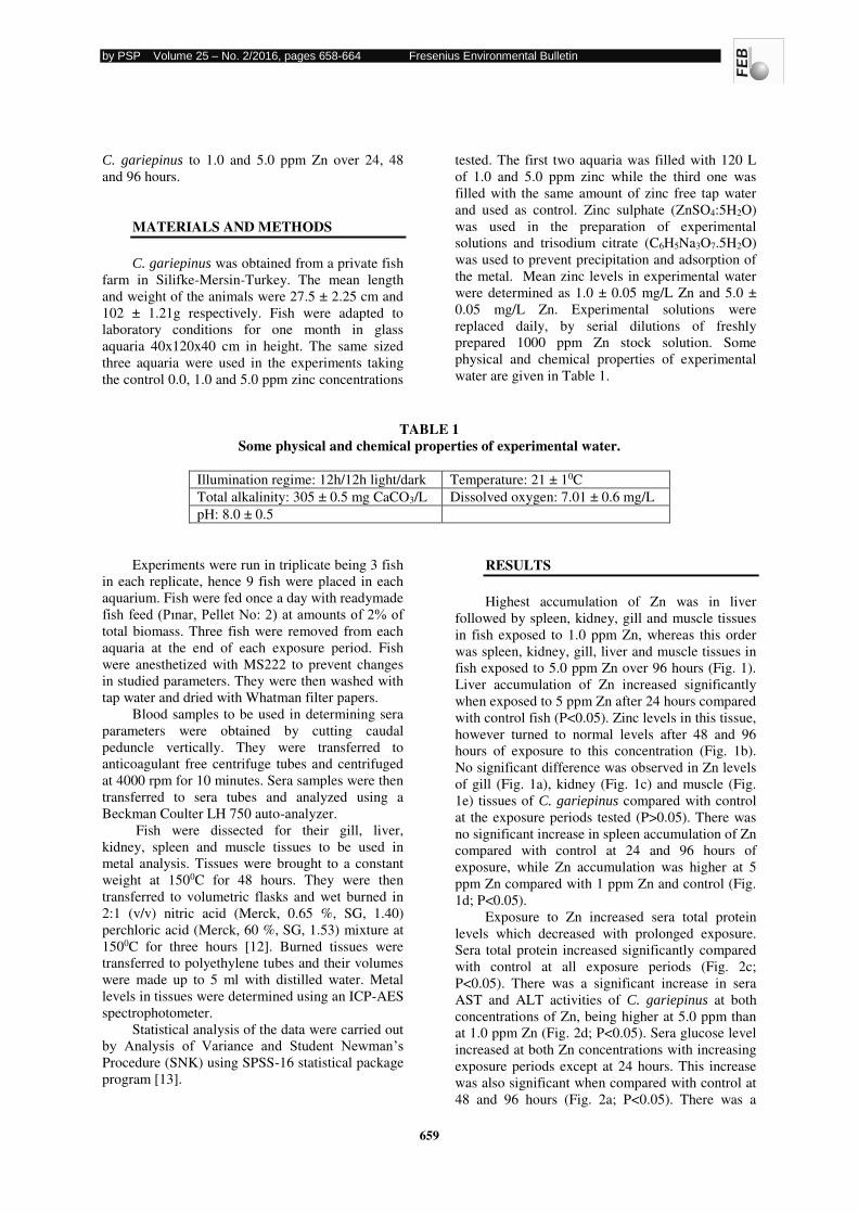
by PSP Volume 25 – No. 2/2016, pages 658-664 Fresenius Environmental Bulletin
659
C. gariepinus to 1.0 and 5.0 ppm Zn over 24, 48
and 96 hours.
MATERIALS AND METHODS
C. gariepinus was obtained from a private fish
farm in Silifke-Mersin-Turkey. The mean length
and weight of the animals were 27.5 ± 2.25 cm and
102 ± 1.21g respectively. Fish were adapted to
laboratory conditions for one month in glass
aquaria 40x120x40 cm in height. The same sized
three aquaria were used in the experiments taking
the control 0.0, 1.0 and 5.0 ppm zinc concentrations
tested. The first two aquaria was filled with 120 L
of 1.0 and 5.0 ppm zinc while the third one was
filled with the same amount of zinc free tap water
and used as control. Zinc sulphate (ZnSO4:5H2O)
was used in the preparation of experimental
solutions and trisodium citrate (C6H5Na3O7.5H2O)
was used to prevent precipitation and adsorption of
the metal. Mean zinc levels in experimental water
were determined as 1.0 ± 0.05 mg/L Zn and 5.0 ±
0.05 mg/L Zn. Experimental solutions were
replaced daily, by serial dilutions of freshly
prepared 1000 ppm Zn stock solution. Some
physical and chemical properties of experimental
water are given in Table 1.
TABLE 1 Some physical and chemical properties of experimental water.
Illumination regime: 12h/12h light/dark Temperature: 21 ± 10C
Total alkalinity: 305 ± 0.5 mg CaCO3/L Dissolved oxygen: 7.01 ± 0.6 mg/L
pH: 8.0 ± 0.5
Experiments were run in triplicate being 3 fish
in each replicate, hence 9 fish were placed in each
aquarium. Fish were fed once a day with readymade
fish feed (Pınar, Pellet No: 2) at amounts of 2% of total biomass. Three fish were removed from each
aquaria at the end of each exposure period. Fish
were anesthetized with MS222 to prevent changes
in studied parameters. They were then washed with
tap water and dried with Whatman filter papers.
Blood samples to be used in determining sera
parameters were obtained by cutting caudal
peduncle vertically. They were transferred to
anticoagulant free centrifuge tubes and centrifuged
at 4000 rpm for 10 minutes. Sera samples were then
transferred to sera tubes and analyzed using a
Beckman Coulter LH 750 auto-analyzer.
Fish were dissected for their gill, liver,
kidney, spleen and muscle tissues to be used in
metal analysis. Tissues were brought to a constant
weight at 1500C for 48 hours. They were then
transferred to volumetric flasks and wet burned in
2:1 (v/v) nitric acid (Merck, 0.65 %, SG, 1.40)
perchloric acid (Merck, 60 %, SG, 1.53) mixture at
1500C for three hours [12]. Burned tissues were
transferred to polyethylene tubes and their volumes
were made up to 5 ml with distilled water. Metal
levels in tissues were determined using an ICP-AES
spectrophotometer.
Statistical analysis of the data were carried out
by Analysis of Variance and Student Newman’s Procedure (SNK) using SPSS-16 statistical package
program [13].
RESULTS
Highest accumulation of Zn was in liver
followed by spleen, kidney, gill and muscle tissues
in fish exposed to 1.0 ppm Zn, whereas this order
was spleen, kidney, gill, liver and muscle tissues in
fish exposed to 5.0 ppm Zn over 96 hours (Fig. 1).
Liver accumulation of Zn increased significantly
when exposed to 5 ppm Zn after 24 hours compared
with control fish (P<0.05). Zinc levels in this tissue,
however turned to normal levels after 48 and 96
hours of exposure to this concentration (Fig. 1b).
No significant difference was observed in Zn levels
of gill (Fig. 1a), kidney (Fig. 1c) and muscle (Fig.
1e) tissues of C. gariepinus compared with control
at the exposure periods tested (P>0.05). There was
no significant increase in spleen accumulation of Zn
compared with control at 24 and 96 hours of
exposure, while Zn accumulation was higher at 5
ppm Zn compared with 1 ppm Zn and control (Fig.
1d; P<0.05).
Exposure to Zn increased sera total protein
levels which decreased with prolonged exposure.
Sera total protein increased significantly compared
with control at all exposure periods (Fig. 2c;
P<0.05). There was a significant increase in sera
AST and ALT activities of C. gariepinus at both
concentrations of Zn, being higher at 5.0 ppm than
at 1.0 ppm Zn (Fig. 2d; P<0.05). Sera glucose level
increased at both Zn concentrations with increasing
exposure periods except at 24 hours. This increase
was also significant when compared with control at
48 and 96 hours (Fig. 2a; P<0.05). There was a
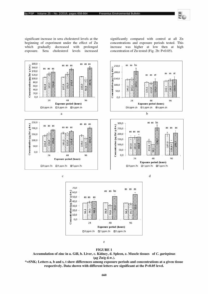
by PSP Volume 25 – No. 2/2016, pages 658-664 Fresenius Environmental Bulletin
660
significant increase in sera cholesterol levels at the
beginning of experiment under the effect of Zn
which gradually decreased with prolonged
exposure. Sera cholesterol levels increased
significantly compared with control at all Zn
concentrations and exposure periods tested. This
increase was higher at low then at high
concentration of Zn tested (Fig. 2b: P<0.05).
a b
c d
e
FIGURE 1 Accumulation of zinc in a. Gill, b. Liver, c. Kidney, d. Spleen, e. Muscle tissues of C. gariepinus
(µg Zn/g d.w.). *=SNK; Letters a, b and s, t show differences among exposure periods and concentrations at a given tissue
respectively. Data shown with different letters are significant at the P<0.05 level.
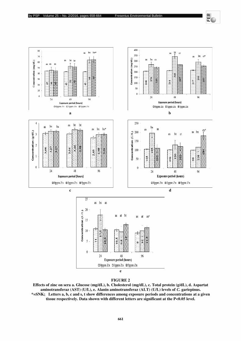
by PSP Volume 25 – No. 2/2016, pages 658-664 Fresenius Environmental Bulletin
661
a b
c d
e
FIGURE 2 Effects of zinc on sera a. Glucose (mg/dL), b. Cholesterol (mg/dL), c. Total protein (g/dL), d. Aspartat
aminotransferaz (AST) (U/L), e. Alanin aminotransferaz (ALT) (U/L) levels of C. gariepinus. *=SNK; Letters a, b, c and s, t show differences among exposure periods and concentrations at a given
tissue respectively. Data shown with different letters are significant at the P<0.05 level.
by PSP Volume 25 – No. 2/2016, pages 658-664 Fresenius Environmental Bulletin
662
DISCUSSION
There was no mortality C. gariepinus exposed
to 5.0 ppm Zn over 96 hours which was probably
due to short exposure periods and low metal
concentrations. Previously observed behavioral
differences were also true for C. gariepinus
exposed to zinc at the beginning of experiments
[14-15].
Highest accumulation of Zn was in liver tissue
of C. gariepinus followed by spleen, kidney, gill
and muscle tissues in fish exposed to 1.0 ppm Zn
whereas this order was spleen, kidney, gill, liver
and muscle tissues in 5.0 ppm Zn exposed fish.
Accumulation of Zn and Cu was higher in the liver
tissue of Scyliorhinus canicula whereas the lowest
accumulation was in muscle tissue [16]. These
difference among the tissues in accumulating
metals can be explained by discrepancies of
metabolic activities of these tissues. Although Zn is
a trace element excess levels of this metal are also
toxic and are carried to liver for detoxification and
to kidneys for excretion.
Gills are the target organs in accumulating
metals since they are in direct contact with the
external media [10]. Short exposure to high
concentrations of Zn resulted in higher gill and liver
accumulation in C. lazera and Tilapia zillii [17] and
in Channa punctatus [18]. No significant difference
was observed in Zn levels of gill, which might be
due to the low concentration and short exposure
periods.
Metals entering from gills are firstly
transferred to liver by the circulatory system, and
when the carrying capacity of liver is exceeded,
they are transferred and stored in metabolically
active tissues, especially in kidney and spleen [19].
Cicik [20] reported liver accumulation of Cu and
Zn accumulation was higher compared to gill and
muscle tissues in C. carpio. Puntius parrah
exposed to 0.9.mg/L Zn over 1, 3, 7, 14, and 28
days accumulated higher levels of Zn in liver,
followed by kidney, gill and muscle tissues [21].
Zinc accumulation in liver increased on days 1 and
3, remained unchanged on day 7 and increased
again on the following days. Liver accumulation of
zinc in 5.0 ppm Zn exposed C. gariepinus increased
compared with control after 24 hours of exposure
and returned to control levels on prolonged
exposure probably due to activation of
detoxification mechanisms.
Spleen accumulation of Zn was highest
compared with the other tissues studied in
C. gariepinus exposed to 5.0 ppm Zn. Studies
carried out with other fish species have also shown
that spleen accumulate high levels of this metal
[22]. Muscle, although not an active tissue in
accumulating metals, plays an important role in
transferring metals to higher trophic levels through
food chain at more concentrated forms. Muscle
accumulation of metals was generally low
compared with liver, kidney and gill tissues as
shown by previous studies which was also shown to
be true in the present study [23-24]. Muscle is an
important tissue for carrying the metals to upper
trophic levels, although it is not an effective tissue
in metal accumulation. Although muscle is not an
effective tissue in binding metals it is important to
know metal levels in this tissue as far as food chain
and human health is concerned.
Heavy metals above given concentrations
activate stress conditions in fish as other stress
factors, such as temperature and anaerobic
conditions, which in turn increases the need for
energy. The increase in energy demand stimulates
the release of glucocorticoids such as cortisol,
epinephrine, and catecholamine causing
mobilization of liver and muscle glycogen by
glycogenolysis and result in hyperglycemia. Copper
increases sera glucose and cortisol levels in Salmo
trutta depending on exposure concentration and
period [25]. McLeay [26] reported that sera glucose
levels increased in Oncorhynchus mykiss exposed
to zinc for 7 days. Sera glucose levels of
C. gariepinus exposed to 1.0 and 5.0 ppm Zn
increased with exposure period except for 24 hours.
This might result from stimulation of
glycogenolysis in liver and muscle depending upon
the energy demand under the effect of zinc.
Cholesterol is the main structural component
of lipoproteins, bile acids and steroid hormones.
Effects of heavy metals on cholesterol levels in fish
varies between fish species and metals tested. Sera
cholesterol levels increased in Oreochromis
niloticus exposed to Ag, Zn, Cr, Cu and Cd singly
[27] while long term effect of methyl mercury and
lead decreased sera cholesterol levels in Lepomis
macrochirus [28] and in Prochilodus lineatus [29]
respectively. Short term exposure to Zn increased
sera cholesterol levels of C. gariepinus whereas its
level decreased with increasing periods. Variations
in sera cholesterol levels under the effect of Zn
might be due to tissue damage caused by the metal,
breakdown in cholesterol synthesis and/or the use
of cholesterol in the synthesis of steroid hormones.
Trace elements are transported between
various tissues by binding to proteins such as
albumin, globulin and ceruloplasmin. Sera total
protein levels of O. mykiss increased exposed to
copper for 15 and 30 days [30]. Sera total protein
levels of Cyprinus carpio increased under the effect
of Cu and Zn [31] and in T. zillii and C. lazera
exposed to Zn [16]. These increases, however, were
not continuous. Sera total protein levels of
by PSP Volume 25 – No. 2/2016, pages 658-664 Fresenius Environmental Bulletin
663
C. gariepinus increased on the 24th hour of
exposure to Zn and decreased with increasing
periods. The increase in synthesis of metal binding
proteins and time depended increase in protein
catabolism might explain these variations.
Heavy metals not only induces stress
conditions in fish but also cause tissue damages.
Stress conditions in fish increase energy
requirements which is derived primarily from
carbohydrates, such as glucose and from non-
carbohydrate sources, such as proteins and lipids,
through gluconeogenic enzymes, namely AST and
ALT. The levels of gluconeogenic enzymes are low
under normal conditions. Sera AST and ALT
activities of O. mykiss increased on the 15 and 30
days of exposure to cadmium [32]. Zinc increased
sera AST and ALT activities in O. niloticus at both
short and long exposure periods [33]. Sera AST and
ALT activities increased to higher levels at 5.0 ppm
than at 1.0 ppm Zn concentration in C. gariepinus.
The results of the present study revealed that
zinc even at low concentrations and exposure
periods can result in tissue accumulation and cause
variations in sera glucose, cholesterol, total protein
levels, AST and ALT activities which all can be
used in determining Zn toxicity to the species
mentioned. It was concluded that the studied zinc
concentrations caused significant alterations in the
carbohydrate and protein metabolism by effecting
sera parameters.
REFERENCES
[1] Naito, W., Kamo, M., Tsushima, K. and
Iwasaki, Y. (2010) Exposure and risk
assessment of zinc in Japanese surface waters.
Sci. Total. Environ. 408(20), 4271–4284.
[2] Handy, R.D. (2003) Chronic effects of copper
exposure versus endocrine toxicity: two sides
of the same toxicological process. Comp.
Biochem. Physiol. 135A, 25-38.
[3] Valee, B.L. and Falchuk, K. (1993) The
biochemical basis of zinc physiology. Physiol.
Rev. 73, 79-118.
[4] Kozlowski, H., Janicka-Klos, A., Brasun, J.,
Gaggelli, E., Valensin, D. and Valensin, G.
(2009) Copper, iron, and zinc ions
homeostasis and their role in
neurodegenerative disorders (metal uptake,
transport, distribution and regulation). Coord.
Chem. Rev. 253, 2665–2685.
[5] Galvez, F., Nebb, N., Hogstrand, C. and Wood
C.M. (1998) Zinc binding to the gills of
Rainbow Trout: the effect of long-term
exposure to sublethal zinc. J. Fish. Biol. 52,
1089-1104.
[6] Shaw, J.R., Dempsey, T.D., Chen, C.Y.,
Hamilton, J.W. and Folt, C.L. (2006)
Comparative toxicity of cadmium, zinc and
mixtures of cadmium and zinc to daphnids.
Environ. Toxicol. Chem., 25,182–189.
[7] Dange, A.D. (1986) Changes in carbohydrate
metabolism in Tilapia Oreochromis
mossambicus, during short-term exposure to
different types of pollutants. Environ Pollut
41, 165-177.
[8] Kuşatan, Z. and Cicik, B. (2004) Clarias lazera
(Valenciennes, 1840)’da kadmiyum’un solungaç, karaciğer, böbrek, dalak ve kas dokularındaki birikimi. SDÜ. Eğirdir Su Ürünleri Fakültesi Dergisi, 2(12), 59-66.
[9] Tunçsoy, M., Duran, S., Ay, Ö., Cicik, B. and
Erdem, C. (2015) Effects of copper and lead
applied singly and in mixture with chitosan on
some sera parameters of Clarias gariepinus.
Fresen. Environ. Bull. 24(9A), 3029-3034.
[10] Cowey, C.B. and Walton, M.J. (1988)
Intermediary metabolism in fish nutrition 2nd
edition. Academic Press, San Diego, pp 259-
329.
[11] Heath, A.G. (1995). Water pollution and fish
physiology. CRC press, Florida, USA.
[12] Muramoto, S. (1983) Elimination of copper
from cu-contaminated fish by long- term
exposure to edta and freshwater. J. Environ.
Sci. Health. A. 18(3), 455-461.
[13] Sokal, R.R. and Rohlf, F.J. (1995) Biometry:
the principles and practice of statistics in
biological research. 3rd edition. W.H. Freeman
and Co., New York.
[14] Duran, S. and Erdem C. (2014) Effects of
sublethal concentration of copper, zinc and
cadmium, applied singly and in mixture, on
some hematological parameters of
Oreochromis niloticus (L., 1758). Fresen.
Environ. Bull. 22(10A), 2977-2980.
[15] Tunçsoy, M. and Erdem, C. (2014)
Accumulation of copper, zinc and cadmium in
liver, gill and muscle tissues of Oreochromis
niloticus exposed to these metals separately
and in mixture. Fresen. Environ. Bull. 23(5),
1143-1149.
[16] Sanpera, C., Vallribera, M. and Crepo, S.
(1983) Zn, Cu and Mn levels in the liver of the
dogfish exposed to Zn. Bull. Environ.
Contam. Toxicol. 31, 415-417.
[17] Hilmy, A.M., El-Domiaty, N.A., Daabees,
A.Y. and Abdel Latife H.A. (1987) Some
physiological and biochemical indices of zinc
toxicity in two freshwater fish, Clarias lazera
and Tilapia zillii. Comp. Biochem. Physiol.
87C(2), 297-301.
by PSP Volume 25 – No. 2/2016, pages 658-664 Fresenius Environmental Bulletin
664
[18] Shukla, V., Dhankhar, M., Prakash, J. and
Sastry, K.V. (2007) Bioaccumulation of Zn,
Cu and Cd in Channa punctatus. J. Environ.
Biol. 28(2), 395-397.
[19] Cousins, R.J. (1985) Absorption, transport and
hepatic metabolism of copper and zinc:
special reference to metallothionein and
ceruloplasmin. Physiol. Rev. 65, 238–309.
[20] Cicik, B. (2003) Bakır-çinko etkileşiminin sazan (Cyprinus carpio)’ın karaciğer, solungaç ve kas dokularındaki metal birikimi üzerine etkileri. Ekoloji 12(48), 32-36.
[21] Ciji, P.P. and Nandan, S.B. (2014) Toxicity of
copper and zinc to Puntius parrah (Day,
1865). Mar. Environ. Res. 93, 38-46.
[22] Flos, R., Caritat, A. and Balasch, J. (1979)
Zinc content in organs of dogfish
(Scyliorhinus canicula L.) subjected to
sublethal experimental aquatic zinc pollution.
Comp. Biochem. Physiol. 64C, 77- 81.
[23] Zyadah, M. and Chouikhi, A. (1999) Heavy
metal accumulation in Mullus barbatus,
Merluccius merluccius and Boops boops fish
from Aegean Sea, Turkey. Int. J. Food. Sci.
Nutr. 50, 429–434.
[24] Cicik, B., Ay, Ö. and Karayakar, F. (2004)
Effects of lead and cadmium interactions on
the metal accumulation in tissue and organs of
the Nile Tilapia (Oreochromis niloticus). Bull.
Environ. Contam. Toxicol. 72, 141-148.
[25] Nemcsok, J. and Hughes, G.M. (1988) The
effect of copper sulphate on some biochemical
parameters of Rainbow Trout. Environ. Pollut.
49, 77–85.
[26] McLeay, D.J. (1977) Development of a blood
sugar bioassay for rapidly measuring stressful
levels of pulpmill effluents in salmonid fish. J.
Fish. Res. Bd. Can. 34, 477-485.
[27] Öner, M., Atlı, G. and Canlı, M. (2007). Changes in serum biochemical parameters of
freshwater fish oreochromis nilotıcus following prolonged metal (Ag, Cd, Cr, Cu,
Zn) exposures. Environ. Toxicol. Chem.
27(2), 360–366.
[28] Dutta, H.M. and Haghighi, A.Z. (1986)
Methylmercuric chloride and serum
cholesterol level in the Bluegill (Lepomis
macrochirus). Bull. Environ. Contam.
Toxicol. 36, 181-185.
[29] Martinez, C.B.R., Nagae, M.Y., Zaia, C.T.B.V.
and Zaia, D.A.M. (2004) Acute morphological
and physiological effects of lead in the
neotropical fish Prochilodus lineatus. Braz. J.
Biol. 64(4), 797-807.
[30] Heydarnejad, M.S., Khosravian-hemami, M.,
Nematollahi, A. and Rahnama, S. (2013)
Effects of copper at sublethal concentrations
on growth and biochemical parameters in
rainbow trout (Oncorhynchus mykiss). Int.
Rev. Hydrobiol. 98, 71-79.
[31] De Smet, H. and Blust, R. (2001) Stress
responses and changes in protein metabolism
in Carp Cyprinus carpio during cadmium
exposure. Ecotoxicol. Environ. Safe. 48(3),
255-262.
[32] Heydarnejad, M.S., Khosravian-hemami, M.
and Nematollahi, A. (2013) Effects of
cadmium at sub-lethal concentration on
growth and biochemical parameters in
rainbow trout (Oncorhynchus mykiss). Irish
Vet. J. 66(11), 2-7.
[33] Younis, E.M., Abdel-Warith, A.A. and Al-
Asgah, N.A. (2012) Hematological and
enzymatic responses of nile tilapia
Oreochromis niloticus during short and long
term sublethal exposure to zinc. Afr. J.
Biotechnol. 11(19), 4442-4446.
Received: 13.06.2015 Accepted: 04.12.2015 CORRESPONDING AUTHOR
Mustafa Tuncsoy University of Çukurova
Faculty of Science and Letters
Biology Department
01330, Balcalı Adana Turkey
e-mail: [email protected]
by PSP Volume 25 – No. 2/ 2016, pages 665-666 Fresenius Environmental Bulletin
665
AUTHOR INDEX
A
Aktaş, A. 612 Allabashi, R. 525
Aouchiche, F. 580 Arman, H. 409
Ay, Ö. 658 Aysun, G. U. 444
B
Ballı, E. 612 Battal, D. 612
Banu, Ö. 444 Baraj, E. 525
Beibei, Z. 373 Benmounah, A. 580
C
Canal, S. B. 623 Cao, W. 647
Ceribasi, G. 565 Chao, D. 373
Chao, H. 384 Chen, W. 602
Chen, Y. 534, 548 Chen, Z. 391
Cicik, B. 658 Çömelekoğlu, Ü. 612
D
Demirel, I. H. 409 Dian, Y. 373
Dogan, E. 565 Duran, S. 658
Dursun, A. F. 444
E
Encu, T. 623 Erdem, C. 658
Eroğlu, P. 612
F
Fan, Y. 633 Fu, A. 534, 548
G
Gang, Y. 373 Ghomi, M. R. 401
Göney, G. 612 Gong, M. 633
Gozdowski, D. 641 Gündoğdu, M. 623
H
Han, Y. 647 Hao, Y. 647
Hu, B. 517
I
Ikhaddalene, S. 580
J
Jiexia, C. 373 Jun, H. 384
K
Kamel, N. 580 Kang, W. 490
Karagül, I. 612 Kaska, A. 509
Kayıkçı, E. T. 464 Kazancı, S. Z. 464
L
Li, H. 419 Li, W. 534, 548
Lilo, R. 525 Linbo, Q. 384
Liu, D. 391 Liu, L. 490, 647
Liu, X. 490 Lu, Z. 391
by PSP Volume 25 – No. 2/ 2016, pages 665-666 Fresenius Environmental Bulletin
666
M
Ma, F. 588 Mahanpoor 500
Moran, H. H. 429 Moudir, D. 580
Mouheb, Y. 580 Muradoğlu, F. 623
O
Ocakoğlu, K. 612 Özkan, C. 429
Q
Qiming, X. 373
R
Ramazan, M. 444 Rui, M. 647
Rui, Y. 647
S
Serencam, U. 409 Shehu, A. 525
Shi, X. 588 Shokri, A. 500
Söğüt, F. 612 Song, G. 419
Songur, M. 409 Sonmez, O. 565
Soodbar, D. 500
T
Tang, X. 647 Tatlı, S. 429
Tunca, H. 429 Tuncsoy, M. 658
Türkseven, C. H. 612
V
Vasjari, M. 525
W
Wang, H. 391 Wang, S. 453
Wang, Y. 490, 517 Wangsheng, C. 384
Wei, C. 453
X
Xiao, W. 490 Xiu, L. 602
Xu, C. 419, 453
Y
Yalın, S. 612 Yaman, S. 612
Yan, Y. 517 Yesilbudak, B. 658
Yıldırımcan, S. 612 Yin, C. 490
Yuksel, I. 409 Yurui, D. 384
Z
Zhang, B. 453 Zhang, H. 633
Zhang, J. 490 Zhang, W. 419, 602
Zaho, B. 588 Zhou, D. 391
Zhou, P. 419 Zhu, W. 633
Zibouche, F. 580
by PSP Volume 25 – No. 2/2016, pages 667-668 Fresenius Environmental Bulletin
667
SUBJECT INDEX
A
Accumulation 658 Adsorption 588
Alkali catalysts 633 Antioxidant 612
Antioxidant enzyme activity 623 Arid region 548
Artificial neural networks 565 Atmospheric drought 534
B
Batch experiments 517 Bioavailability 453
Biochar 588, 602 Biological control 429
Biomass 588 Botanical insecticide 429
By-products 373
C
Cadmium-contaminated soil 602 Characterization 588
Clarias gariepinus 658 Climate changes 548
Common carp 401 Content 647
Contractility 612 Corn 548
Correlations 641 Correlation analysis 490
Cr(VI) 588 Cyanobacteria 633
D
DNA damage 612
E
ECG 612 EDCs 373
Electron/hole separation 391 EVI 641
F
Farmland soils 490 Fe 580
G
Gasification 633 Green turtle 509
H
Heavy metals 490, 525, 647 Heart 612
Hydropower 409
I
Industrial experiments 384 Inorganic P fraction 517
Interpolation Error 464 Inverse distance weighted 464
L
Langmuir-Hinshelwood 500 Lead stress 623
Lipid peroxidase 623 Loggerhead turtle 509
M
Macro-micro element 623 Maize straw 602
Mechanisms 517 Mitochondrial DNA 509
N
Nanostructures 391 NDVI 641
Nuclear glass 580
O
Organic fertilizer 647 Organic P fraction 517
by PSP Volume 25 – No. 2/2016, pages 667-668 Fresenius Environmental Bulletin
668
Ozonation 373
P 210Pb 444 210Po 444
pH 373 Photocatalytic properties 391
Polymorphism 509 Principal component analysis 490
R
Radioactive waste 580 Renewable energy 409
Rice 602 Risk assessment 490
RRM 419
S
Sequential extraction 517 SEM 580
Sera biochemical parameters 658 Side-effect 429
Silica nanoparticle 612 Sintering flue gas 384
Soil erosion 444 Soil evaporation rate 548
Soil fractions 641 Soil sampling 641
Spatial interpolation 464 Speciation 647
Storage 580 Strawberry 623
Streamflow 565 Street dust 453
Supercritical water 633
T
Temperature Lapse Rate 464 Transpiration rate 548
Trend analysis 565 Trichogramma pintoi 429
W
Water contamination 525 Wuta-tsai 647
X
X-ray diffraction pattern 500 XRD 580
Z
Zinc 658
by PSP Volume 25 – No. 2/2016 Fresenius Environmental Bulletin
FEB- GUIDE FOR AUTHORS
General FEB accepts original papers, review articles, short
communications, research abstracts from the entire
sphere
of environmental-chemistry,-biology,-
microbiology,- technology, -biotechnology and-
management, furthermore, about residueanalysis/
and ecotoxicology of contaminants.
Acceptance or nonacceptance of a contribution will
be decided, as in the case of other scientific
journals, by a board of reviewers.Papers are
processed with the understanding that they have not
been published before (except in form of an abstract
or as a part of a published lecture, review or
thesis);that they are not under consideration for
publication elsewhere; that their publication has
been approved by all co-authors, if any, as well as-
tacitly or explicitly- by the responsible authorities
at the institute where the work has been carried out
and that, if accepted, it will not be published
elsewhere in the same form, in either the same or
another language, without the consent of the
copyright holders.
Language Papers must be written in English. Spelling may
eitherfollow American (Webster) or British
(Oxford) usage but must be consistent. Authors
who are less familiar with the English language
should seek assistance from proficient colleagues in
order to produce manuscripts that are
grammatically and linguistically correct.
Size of manuscript Review articles should not exceed 30 typewritten
pages. In addition up to 5 figures may be included.
Original papers must not exceed 14 typewritten
pages. In addition up to 5 figures may be included.
Short-Communications should be limited to 4
typewrittenpages plus not more than 1 illustration.
Short descriptions of the authors, presentation of
their groups and their research activities (with
photo) should together not exceed I typewritten
page.Short research abstracts should report in a few
brief sentences (one-forth to one page) particularly
significant findings.Short articles by relative
newcomers to the chemical innovation arena
highlight the key elements of their Master and PhD-
works in about I page.
Book Reviews are normally written in-house, but
suggestions for books to review are welcome.
Preparation of manuscript Dear authors,
FEB is available both as printed journal and as
online journal on the web. You can now e-mail
your manuscripts with an attached file. Save both
time and money.To avoid any problems handling
your text please follow the instructions given
below:
When preparing your manuscripts have the formula
K/SS ( Keep It Simple and Stupid) in mind.Most
word processing programs such as MS-Word offera
lot of features. Some of them can do serious harm
to our layout. So please do not insert hyperlinks
and/or automatic cross-references, tables of
contents,references, footnotes, etc
1. Please use the standard format features of your
word processor (such as standard.dotfor MS Word).
2. Please do not insert automatisms or secret link-
ups between your text and your figures or
tables. These features will drive our graphic
department sometimes mad.
3. Please only use two fonts. for text or tables
"Times New Roman" and for graphical
presentations "Arial".
4. Stylesheets, text, tables and graphics in shade of
grey
5. Turn on the automatic language detection
inEnglish (American or British)
6. Please - check your files for viruses before you
send them to us!!
Manuscripts should send to:[email protected]
Thank you very much!
by PSP Volume 25 – No. 2/2016 Fresenius Environmental Bulletin
STRUCTURE OF THE MANUSCRIPT
Title page:The first page of the manuscript should
contain the following items in the sequence given:A
concise title of the paper (no abbreviations)The
names of all authors with at least one first name
spelled out for every author.The names of
Universities with Faculty, City and Country of all
authors.
Abstracts:The second page of the manuscript
should start with an abstract that summarizes
briefly the contents of the paper (except short
communications). Its lenght should not exceed 150-
200 words. The abstract should be as informative as
possible. An extended repetition of the paper's title
is not considered to be an abstract.
Keywords:Below the Summary up to 6 key words
have to beprovided which will assist indexers in
crossindexing your article.
Introduction:This should define the problem and,
if possible, the frame of existing knowledge. Please
ensure that people not working in that particular
field will be able to understand the intention. The
word length of the introduction should be 150 to
300 words.
Materials and methods: Please be as precise as possible to enable other
scientiststo repeat the work.
Results:Only material pertinent to the subject must
be included.Data must not be repeated in figures
and tables.
Acknowledgements:Acknowledgements of
financial support, advice orother kind of assistance
should be given at the end of the text under the
heading "Acknowledgements". The names of
funding organisations should be written in full.
Reference:Responsibility for the accuracy of
references rests with the authors. References are to
be limited in number to those absolutely
necessary.References should appear in numerical
order in brackets and in order of their citation in the
text. They should be grouped at the end of the paper
in numerical order of appearance. Abbreviated titles
of periodicals are to be used according to Chemical
or Biological Abstracts,but names of lesser known
journals should be typed in full.References should
be styled and punctuated according to the following
examples:
ORIGINALPAPERS:
l. Author, N.N. and Author, N.N. (Year) Full title of
the article. Joumal and Volume, first and last page.
BOOK OR PROCEEDING:
2. Author, N.N. and Author, N.N. (Year) Title of
the contribution.
In: Title of the book or proceeding. Volume
(Edition
of klitor-s, ed-s) Publisher, City, first and last page
DOCTORALTHESIS:
3. Author, N.N. (Year) Tille of the thesis,
University and
Faculty, City
UNPUBLISHED WORK:
Papers that are unpublished but have been
submitted to a joumal may be cited with the
joumal's name followed by "in press". However,
this practice is acceptable only if the author has at
least received galley proofs of his paper. In all other
cases reference must be made to”unpublished work" or "personal communication".
Discussion and Conclusion:This part should
interpret the results in reference to the problem
outlined in the introduction and of related
observations by the author/s or others. Implications
for further studies or application may be discussed.
A conclusion should be added if results and
discussion are combined.
Corresponding author:The name of the
corresponding author with complete postal address
Precondition for publishing:
A minimum number of 25 reprints must be
ordered and prepaid. 1 - 4 pp.: 200,- EURO + postage/handling
5 - 8 pp.: 250,- EURO + postage/ handling
more than 8pp: 1.50 EURO/page x number of reprints
+postage/ handling.
The prices are based upon the number of pages in our
journal
layout (not on the page numbers of the submitted
manuscript).
Postage/ Handling: The current freight rate is
Germany 10 €,Europe 18,00 €, International 30 €.VAT: In certain circumstances (if no VAT
registration number exists) we may be obliged to
charge 7% VAT on sales to other EU member
countries.MESAEP and SECOTOX members get a
further discountof 20% (postage/ handling full).