Distributed average consensus with stochastic communication failures
Upload
khangminh22Category
view
1download
0
FEA-BASED METHOD TO PREDICT DYNAMIC TEST
FAILURES OF INDUSTRIAL RUBBER CASTOR
WHEELS
Ampitiyawaththe Vishvajith Wijayasundara
(128413 C)
Dissertation submitted in partial fulfillment of the requirements for the
Master of Engineering in Manufacturing Systems Engineering
Department of Mechanical Engineering
University of Moratuwa
Sri Lanka
November 2016

ii
Declaration
I declare that this is my own work and this thesis/dissertation does not
incorporate without acknowledgement any material previously submitted for a
Degree or Diploma in any other University or institute of higher learning and to the
best of my knowledge and belief it does not contain any material previously
published or written by another person except where the acknowledgement is made
in the text.
Also, I hereby grant to University of Moratuwa the non-exclusive right to
reproduce and distribute my dissertation in whole or in part in print, electronic or
other medium. I retain the right to use this content in whole or part in future works
(such as articles or books)
Signature: Date:
A.V.Wijayasundara (128413c)
The above candidate has carried out research for the Masters Dissertation
under my supervision.
Signature of the supervisor: Date:
Dr. H.K.G Punchihewa
Signature of the supervisor: Date :
Mr. R.K.P.S Ranaweera

iii
Acknowledgment
I would first like to thank my research supervisors Dr. H.K.G Punchihewa and Mr.
R.K.P.S Ranaweera at department of Mechanical Engineering in university of
moratuwa Sri Lanka for their continuous guidance and support provided during this
work.
I would like to thank all other staff of department of Mechanical Engineering in
university of moratuwa Sri Lanka for sharing valuable knowledge with me and for the
guidance given for this work.
I’m very grateful for Elastomeric Engineering Co.Ltd located at NO. 51/54, IDB
Industrial Estate, Horana, Sri Lanka for providing me opportunity and resources to
carry out this research work.
I would like to thank Mr. S.Ranathunga, General Manager, Elastomeric
Engineering Co.Ltd. and other staff members at organization for the valuable support
and information given during the work to make this a success.

iv
Abstract
Castor wheels are used in various applications including industries, hospitals, offices,
shopping trollies, air ports and other material handling applications. These applications
demand different properties from castor wheels, such as dynamic load capacity, high speed
capability, and capability to operate in hot and cold environments. Design of a castor wheel
plays a major role to fulfill those various demands while being competitive in the market.
Dynamic test of castor wheel is one of the main tests done on new castor wheel designs to
evaluate its performance for an application. Due to manual trial and error practice used to test
new designs in dynamic test, wheel development cost and lead time for deliver new castor
wheel designs for new customer requirements is high. In order to evaluate wheel designs in
early stages of development in dynamic test performance, Finite element model was developed
to check castor wheel dynamic performance using combination of finite element analysis
(FEA) techniques and raw material testing.
Initially six samples of castor wheels were selected and dynamic test was carried out on
them at various loads to evaluate temperature development inside the wheel and failure modes.
Two sets of raw material testing, namely uniaxial tensile test and dynamic mechanical analyze
test (DMA), were done on rubber and plastic materials which are used to make castor wheels.
One wheel was selected as a case study to develop FEA model. As first step, 3D static loading
simulation was done for the selected wheel. Total energy rate was defined for wheel in
dynamic motion by data from static test using equations. 2D axisymmetric FEA model was
developed as next step to evaluate temperature development of the castor wheel. Calculated
energy rate was distributed among rubber elements as heat sources combining with DMA
results to predict temperature inside the 2D profile using transient heat. Wheel failure analysis
was carried out by combining predicted temperature profile and static loading case with
temperature dependent properties of materials used. It was defined as a good design if castor
wheel shows higher safety factor in failure simulation. From the case study, step-by-step
method was developed to simulated castor wheel designs and evaluated failure. Four castor
wheels were simulated according to developed model and predicted temperatures were
compared with actual dynamic test temperature to validate the proposed model which showed
good match with practical data. As future work, advanced failure analysis of caster wheels can
be proposed, which should be carried out considering material chemistry and behavioral
changes of materials with heat and fatigue loads.

v
Table of Contents
Declaration ................................................................................................................... ii
Acknowledgment ........................................................................................................ iii
Abstract ....................................................................................................................... iv
List of Figures ........................................................................................................... viii
List of Tables............................................................................................................... xi
1. Introduction .......................................................................................................... 1
1.1. Background ................................................................................................ 1
1.2. Motivation .................................................................................................. 3
1.3. Problem Definition .................................................................................... 5
2. Literature Review ................................................................................................. 9
2.1. Castor Wheel Test Standards ..................................................................... 9
2.2. Physical Test Methods ............................................................................. 13
2.3. Simulation Methods ................................................................................. 14
3. Methodology ....................................................................................................... 20
4. Physical Testing and Results .............................................................................. 24
4.1. Product Testing ........................................................................................ 24
4.1.1. Sample Wheel Selection ............................................................. 24
4.1.2. Dynamic Test .............................................................................. 25
4.1.3. Dynamic Test Results ................................................................. 27
4.2. Raw Material Testing............................................................................... 30
4.2.1. Tensile Test ................................................................................ 30
4.2.2. DMA Test ................................................................................... 33
5. Finite Element Model Development................................................................... 36
5.1. Static Loading .......................................................................................... 36
5.1.1. Mesh Creation ............................................................................ 38

vi
5.1.2. Boundary Conditions .................................................................. 40
5.1.3. Material Models .......................................................................... 42
5.1.4. Solver Setup ................................................................................ 44
5.1.5. Simulation Results ...................................................................... 44
5.2. Total Energy Rate Calculation ................................................................. 47
5.3. Temperature Prediction............................................................................ 49
5.3.1. 2D Model and Mesh Creation .................................................... 50
5.3.2. Heat Generation Rate.................................................................. 50
5.3.3. Thermal boundary conditions ..................................................... 53
5.3.4. Solver setup ................................................................................ 53
5.3.5. Simulation results ....................................................................... 54
5.4. Failure Analysis ....................................................................................... 58
5.4.1. Equivalent Load Calculation ...................................................... 59
5.4.2. 2D simulation Model with Temperature Effects ........................ 61
5.4.3. Simulation results ....................................................................... 63
5.5. Generalized model ................................................................................... 66
6. Validation ........................................................................................................... 73
6.1. Case Study 1 ............................................................................................ 73
6.2. Case Study 2 ............................................................................................ 80
6.3. Case Study 3 ............................................................................................ 88
6.4. Case Study 4 ............................................................................................ 93
7. Discussion ........................................................................................................... 98
8. Conclusions ...................................................................................................... 100
Bibliography ............................................................................................................. 101
Appendix 1 – Sample wheels dynamic test results summary .................................. 105
Appendix 2 – Static loading energy calculation case study 1 .................................. 106

vii
Appendix 3 – Total energy rate calculation case study 1 ........................................ 108
Appendix 4 – Material property data ....................................................................... 110
Appendix 5 – Static load energy calculation case study 2 ....................................... 111
Appendix 6 – Total energy rate calculation case study 2 ........................................ 113
Appendix 7 - Static load energy calculation case study 3 ........................................ 115
Appendix 8 - Total energy rate calculation case study 3 ......................................... 116
Appendix 9 - Static load energy calculation case study 4 ........................................ 117
Appendix 10 - Total energy rate calculation case study 4 ....................................... 119

viii
List of Figures
Figure 1.1: Castor wheels mounted in industrial trolley .............................................. 1
Figure 1.2 : Assembled castor wheel with swivel fork ................................................ 2
Figure 1.3 : Main parts of a castor wheel and materials .............................................. 3
Figure 1.4 : Tests conducted for industrial castors ...................................................... 5
Figure 1.5 : Castor wheel dynamic test apparatus........................................................ 6
Figure 2.1 : Temperature prediction method for pneumatic tyres [9] ........................ 19
Figure 3.1 : FEA model development methodology .................................................. 21
Figure 4.1 : Cross section of a castor wheel............................................................... 24
Figure 4.2 : Castor wheel Dynamic test apparatus (Original in colour) .................... 26
Figure 4.3 : Dynamic test Temperature recorded locations ....................................... 27
Figure 4.4 : Wheel after failure .................................................................................. 27
Figure 4.5 : 160 mm Wheel 450 kg Dynamic test temperature record ...................... 28
Figure 4.6 : Castor wheel temperature development stages ....................................... 29
Figure 4.7 : ASTM D638-Type 1 test piece dimensions ........................................... 30
Figure 4.8 : Polypropylene Stress-Strain graph at 23oC ............................................ 30
Figure 4.9 : Nylon Stress-Strain graph at 23oc ........................................................... 31
Figure 4.10 : ASTMD 412-Type C rubber specimen dimensions ............................. 32
Figure 4.11 : Rubber Stress-Strain graph at 23oc ....................................................... 32
Figure 4.12 : NR-1 & NR-2 Energy loss fraction vs temperature graphs .................. 35
Figure 5.1 : 160 mm Castor wheel dimensions .......................................................... 36
Figure 5.2 : proposed ¼ castor wheel model for FEA ............................................... 37
Figure 5.3 : FEA Elements available for 3D simulation ............................................ 38
Figure 5.4: Convergence analyze for selecting mesh size ......................................... 39
Figure 5.5 : Meshed 3D model of 160 mm Castor wheel .......................................... 40
Figure 5.6 : Meshed model with boundary conditions ............................................... 40
Figure 5.7 : FEA model with loading conditions ....................................................... 41
Figure 5.8 : Material models used in FEA ................................................................. 42
Figure 5.9 : Reaction force vs Solver step graph of 160 mm wheel .......................... 45
Figure 5.10 : Reaction force vs Wheel compression of 160 mm wheel .................... 45
Figure 5.11 : von Mises stress distribution of 160 mm wheel ................................... 46

ix
Figure 5.13 : Stress in Plastic 160 mm wheel (Original in colour) ............................ 46
Figure 5.12 : Stress in rubber 160 mm wheel (Original in colour) ............................ 46
Figure 5.14 : 2D axisymmetric model........................................................................ 50
Figure 5.15 : 2D profile with heat sources applied to relevant elements ................... 51
Figure 5.16 : Castor wheel run cycle graph ............................................................... 52
Figure 5.17: Temperature extracted points from 2D simulation ................................ 54
Figure 5.18 : 160 mm 450 kg FEA simulation temperature prediction ..................... 54
Figure 5.19 : Steady state max temperature profile, 160 mm 450 kg ........................ 55
Figure 5.20 : Rubber inner temperature comparison, 160 mm 450 kg ...................... 56
Figure 5.21 : Plastic inner temperature comparison, 160 mm 450 kg ....................... 57
Figure 5.22 : Plastic outer temperature comparison, 160 mm 450 kg ....................... 57
Figure 5.23 : Rubber outer temperature comparison, 160 mm 450 kg ...................... 58
Figure 5.24 : 160 mm castor wheel 2D profile .......................................................... 59
Figure 5.25 : 160 mm wheel 2D profile stress distortion ........................................... 60
Figure 5.26 : Reaction force on cluster node vs Solver increment ............................ 60
Figure 5.27 : Applied temperature profile, 160 mm wheel, 450 kg loading .............. 62
Figure 5.28 : Reaction force vs Solver step for temperature effect simulation.......... 63
Figure 5.29 : 160 mm castor 450 kg stress profile ..................................................... 64
Figure 5.30 : Example models for 2D profile ............................................................ 66
Figure 5.31 : 3D FEA model of castor wheel ............................................................ 67
Figure 5.32 : 3D FEA model with beam and cluster node at bottom ........................ 68
Figure 5.33 : Temperature prediction 2D model with heat sources ........................... 70
Figure 5.34 : Temperature analyze locations ............................................................. 71
Figure 5.35 : 2D castor wheel FEA profile ................................................................ 71
Figure 6.1 : 160 mm 500 kg load temperature prediction .......................................... 75
Figure 6.2 : Rubber inner temperature comparison, 160 mm 500 kg ........................ 75
Figure 6.3 : Rubber Outer temperature comparison, 160 mm 500 kg ....................... 76
Figure 6.4 : Plastic Inner temperature comparison, 160 mm 500 kg ......................... 76
Figure 6.5 : Plastic Outer temperature comparison, 160 mm 500 kg ........................ 77
Figure 6.6 : Reaction force vs solver step 160 mm wheel 500 kg ............................. 78
Figure 6.7 : 160 mm 500kg load failure analysis ....................................................... 78
Figure 6.8 : 160 mm wheel 500 kg load with temperature stress profile ................... 79

x
Figure 6.9 : 125 mm Castor wheel ............................................................................. 80
Figure 6.10 : 125 mm 125 kg static loading .............................................................. 81
Figure 6.11 : 125mm 125 kg case force vs wheel compression ................................ 81
Figure 6.12 : 125 mm 125 kg temperature prediction setup ...................................... 82
Figure 6.13 : 125 mm 125 kg temperature prediction ................................................ 83
Figure 6.14 : Rubber inner temperature comparison, 125 mm 125 kg ...................... 84
Figure 6.15 : Plastic inner temperature comparison. 125 mm 125 kg ....................... 84
Figure 6.16 : Plastic outer temperature comparison, 125 mm 125 kg ....................... 85
Figure 6.17 : Rubber outer temperature comparison, 125 mm 125 kg ...................... 85
Figure 6.18 : 125 mm wheel 125 kg Force vs solver step.......................................... 86
Figure 6.19 : 125 mm wheel failure analysis ............................................................. 86
Figure 6.20 : 125 mm 125 kg stress distribution at steady state ................................ 87
Figure 6.21 : 100 mm 100 kg case force vs wheel compression ............................... 88
Figure 6.22 : 100 mm 100 kg temperature prediction setup ...................................... 89
Figure 6.23 : Rubber inner temperature comparison, 100mm 100 kg ....................... 90
Figure 6.24 : Plastic inner temperature comparison. 100 mm 100 kg ....................... 90
Figure 6.26 : Plastic outer temperature comparison, 100 mm 100 kg ....................... 91
Figure 6.25 : Rubber outer temperature comparison, 100 mm 100 kg ...................... 91
Figure 6.28 : 100 mm 100 kg stress distribution at steady state ................................ 92
Figure 6.29 : 200 mm 550 kg case force vs wheel compression ............................... 93
Figure 6.30 : 200 mm 550 kg temperature prediction setup ...................................... 94
Figure 6.31 : Rubber inner temperature comparison, 200 mm 550 kg ...................... 95
Figure 6.32 : Plastic inner temperature comparison. 200 mm 550 kg ....................... 95
Figure 6.33 : Plastic outer temperature comparison, 200 mm 550 kg ....................... 96
Figure 6.34 : Rubber outer temperature comparison, 200 mm 550 kg ...................... 96
Figure 6.35 : 200 mm 550 kg stress distribution at steady state ................................ 97

xi
List of Tables
Table 4.1 : Sample Castor wheels and selected test loads ......................................... 25
Table 4.2 : Plastic material tensile test results ........................................................... 31
Table 4.3 : DMA test oscillation frequency ............................................................... 34
Table 5.1 : Max stress in plastic vs Element size ....................................................... 39
Table 5.2 : 160 mm wheel, 450 kg static load safety factor....................................... 47
Table 5.3 : Correction factor calculation.................................................................... 48
Table 5.4 : Total energy rate distribution ................................................................... 51
Table 5.5 : Material properties for thermal simulation .............................................. 53
Table 5.6 : Nylon Tensile data variation with temperature ........................................ 61
Table 5.7 : Polypropylene Tensile data variation with temperature .......................... 62
Table 5.8 : 160 mm 450 kg wheel safety factor ......................................................... 64
Table 6.1 : Element energy rate in 160 mm 500 kg case ........................................... 74
Table 6.2 : 160 mm 500 kg wheel safety factor ......................................................... 79
Table 6.3 : 125 mm 125 kg case static loading stress ................................................ 81
Table 6.4 : 125 mm 125 kg case total energy distribution ......................................... 83
Table 6.5 : 125 mm 125 kg safety factor ................................................................... 87
Table 6.6 : 100 mm 100 kg case static loading stress ................................................ 88
Table 6.7 : 100 mm 100 kg safety factor ................................................................... 92
Table 6.8 : 200 mm 550 kg case static loading stress ................................................ 93
Table 6.9 : 200 mm 550 kg safety factor ................................................................... 97

1
1. Introduction
1.1. Background
Castor wheels are mainly used as a tool that makes object movement easy. They
are un-driven wheels which are designed to be mounted to a bottom of a larger object
so that object can be moved easily. They can be found in various applications around
the world such as in Industrial applications, shopping trollies, office chairs, air ports,
hospitals and other various material handling equipment. These various applications
demand various performance and properties from castor wheels. High capacity heavy
duty castors are used in many industrial applications for continuous use under heavy
loads such as platform trucks, industrial carts, and automated material handling lines.
Castor wheels used in air ports are designed to withstand heavy dynamic and impact
loads. Furniture castors are treated as light load castors but still should consider time
to time extreme loading conditions and environmental conditions which may occur in
practical application. Castor wheels used in hospitals are premium castors which gives
comfortable ride and low noise in applications. Some castor wheels are designed to
conduct electricity while moving the object fitted.
To cater all these application demands, castor wheels are available in various sizes
and designs. Castor wheels are made from various materials such as Rubber,
Polyurethane, Nylon, Aluminum and Stainless steel for various types of applications
in various types of designs.
Figure 1.1: Castor wheels mounted in industrial trolley
Source: https://www.exportersindia.com/punamenterprises-163389.htm

2
A castor wheel is defined as “small wheel on a swivel, attached under a piece of
furniture or other heavy object to make it easier to move” [1] . These wheels are made
from various materials using moulding, forming, matching and assembling methods to
form the final castor wheel.
Forks are made from steel or aluminum most of the time with bearings for make it
easy to rotate. In general, wheel part can be divided in to three main parts named as
outer ring, center part and bearing. Outer ring which is in contact with the floor,
manufactured in flexible material like rubber, polyurethane or thermoplastic rubber to
get comfort and smooth running of the wheel. Most of the time outer ring is made from
moulding method such as compression moulding or injection moulding according to
material. Polypropylene is used as center material for light duty Castor Wheels. Nylon,
Steel, cast iron or Aluminum is used as center material for heavy duty wheels for
different applications. Various methods such as forging, casting, injection moulding
and machining are used to make center part according to material used. Summary of
general material used to make castor wheels are given on Figure 1.3 both roller type
and ball type bearings are used in castor wheels according to applications.
Figure 1.2 : Assembled castor wheel with swivel fork
Source: https://www.tente.com/us-us/

3
Center
Polypropylene (PP)
Nylon (PA6)
Steel
Aluminum
Bearing
Ball Bearing
Roller Bearing
Plain Bearing
Outer Ring
Rubber
Polyurethane
Thermoplastic vulcanize
Thermoplastic urethane
1.2. Motivation
Rubber industry started in Sri Lanka 1876 with planting of rubber trees in
Henerathgoda Botanical Gardens- Colombo. Now a days Sri Lanka is one of reputed
supplier of rubber value-added products for the world market. Sri Lanka Rubber
product industry is composed of about 4,530 manufacturing organizations of small,
medium, and large-scale industries. Main products manufactured and exported from
Sri Lanka are rubber solid tyres, pneumatic tyres, rubber gloves, rubber mats, rubber
castor wheels and rubber bands which brings in foreign currency to Sri Lanka. In 2014
rubber finished products industry earned an export income of US$ 889 Million and
provided direct and indirect employment opportunities to over 300,000 persons [2].
When considered about competition in world market, other Asian countries such as
china, India, Thailand, Indonesia, Malaysia, Vietnam are main competitors for Sri
Lankan rubber products.
Castor wheels which are made from rubber material are one of those value-added
rubber products which accounted for about US$ 50 Million in year 2014. Several
Figure 1.3 : Main parts of a castor wheel and materials
Source: https://www.tente.com/us-us/

4
castor wheel manufactures are located in Sri Lanka who mainly make rubber castor
wheels. Sri Lankan made rubber castor wheels are very popular in the world market
for their high quality, smooth and reliable operations. These are mostly used in various
applications mainly including heavy and light duty industrial applications all around
the world [2], [3].
Castor wheel market is very competitive with lots of wheel suppliers around the
world including mentioned china, India, Thailand, Indonesia, Malaysia, Vietnam
countries. To gain new market share and maintain existing market level, castor wheel
manufacturers are always searching ways to minimize their costs and improve
performance of their castor wheels. Customers are looking to develop customized
castor wheels for their own applications with better performance and minimum cost.
In average five to ten new inquiries about castor wheel new developments are given to
one castor wheel manufacturer per month which suggest this industry is very dynamic
industry. Most of inquiries are new applications in new material handling
developments, new machines, high or low temperature applications, premium
applications such as hospitals, sports items with new improvements. Lots of
developments happening in material handling, castor forks, breaks in castors,
automated vehicles, air ports, hospital equipment which constantly demands new
castor wheel designs. To develop castor wheels low cost and to deliver intended
application, castor wheels must be designed and developed in optimized manner. Lots
of designs considerations and options are considered when designing a new design for
a castor wheel. Lack of proper standardized method to evaluate designs of castor
wheels in design stage was main problem in Sri Lankan castor wheel industry. Most
companies do a sample production and do physical testing to evaluate design
performance of various proposal designs which consumes time and cost.
In this research work focus is to develop a model to determine performance of a
castor wheel design in early design stage so designers can do better designs by
evaluating several design options and select best option before going in to sample trial
and error stage.

5
Industrial castor wheel testing
Static Tests
Initial Wheel Play Test
Conductivity Test
Static Load test
Side Load test
Dynamic Tests
Dynamic loading test
1.3. Problem Definition
When new castor wheel designs are done, it is necessary to evaluate wheel
performance under defined conditions to qualify the new design for a given
application. Even in day to day productions randomly castor wheels are tested to
evaluate performance of castor wheel and ensure quality of supply by castor wheel
manufacturers. To evaluate the performance of the castor wheels, standard test
methods are developed by international bodies [4], [5], [6]. New designs of castor
wheels are tested under defined international test method by manufacture to ensure its
performance in the application. For castor wheel testing, wheels are categorized as,
• Furniture Chair Casters
• Industrial Casters
• Institutional and Medical Equipment Casters
In this study standard used to test industrial castors wheels below 4 km/h was
considered to test wheel designs [6]. Several tests are listed under industrial castor
wheels, tests which are related to wheel part can be categorized as Static tests and
dynamic tests of castor wheels.
Performance of a new castor wheel design in static test can be evaluated Figure 1.4 : Tests conducted for industrial castors

6
Applied load
Castor Wheel with fork
Rotatable Drum
Static tests can be performed by available simple simulations methods or raw
material testing methods. But performance evaluation of a new castor wheel design in
dynamic test is hard task for simple simulation and material testing. There is no proper
defined simulation method to evaluate castor wheel performance under dynamic load
application, because it involves complex parameters like material analyze, viscoelastic
hysteresis energy, heat buildup in the rubber wheel and material property variations
due to temperature [7], [8] .
In the dynamic test castor wheel is mounted on to a rotatable drum and a defined
load is applied to the wheel. Then drum is rotated to a given speed for a given defined
time period making the wheel to rotate with the load. Castor wheel should pass this
test without any failures. Pass criteria for the wheel is defined as “No permanent
deformation should happen in castor wheel which adversely affects performance” [6].
This Standard castor wheel test method is given under international standard. If a
wheel passed this test it is accepted that wheel will perform in the real-world
application.
During the dynamic test, it was observed that most of the wheels were failed at
the center part of the castor wheel. When wheel is rotated, given location of rubber
Figure 1.5 : Castor wheel dynamic test apparatus

7
outer ring is continuously loaded and unloaded resulting heat buildup inside the rubber
which is commonly known as hysteresis heat buildup [9]. Then this heat is also
absorbed by the center part of the castor wheel resulting to reduce its capability to hold
against applied load. Then with time it was observed that center part was melted and
resulted to failure.
Evaluation of dynamic test performance of a new castor wheel in design stage is
important to develop optimized designs with lowest materials for a given application.
Optimized design will result in low cost high performance wheel which will generate
new markets for castor wheel manufacturers. When considered about material
consumption also its always ecofriendly to develop products with minimum weight.
In average five to ten new inquiries are received by manufactures per month to
develop castor wheels for various applications. As first step a basic design of castor
wheel is done or existing wheel design is used for initial costing. Optimization of
wheel design is not considered in this step hence most of times higher price is offered
to customer than actually required. Because of that higher risk is there to lose business
to another competitor. Two to three days are spent on this for costing.
If customer is positive next step is to develop sample wheels for customer
approval which is done by trial and error method. Several moulds will be developed
and various material trials will be done on this moulds also to identify best design.
These additional trials consume additional development time and approximately 70%
of total development cost. If trials are not successful or any improvements are needed,
another mould should be developed and trials should be repeated until satisfactory
results are obtained in product testing such as dynamic test and others. In average
castor wheel development time can range from 1.5 to 3 months’ time based on number
of trials. Development cost is high due to additional mould and materials physical
trials. Because of this method very few design options can be considered in
development also which limit the opportunity to develop best design for a given
application.
Requirement is to develop a finite element simulation method to simulate castor
wheel dynamic test conditions in design stage and evaluate various designs. Through

8
this simulation model wheel manufacturing companies are able develop new castor
wheel designs in optimized manner to a given application with less cost and lead time.
Only wheels made from rubber outer rings and plastic centers (PP and PA6) will be
studied in this research work since these wheels are the main products which are
manufactured in Sri Lanka.
Aim of this research is to develop a finite element model to evaluate castor wheel
designs for failures in dynamic testing. Objectives are to,
• Identify of parameters to be used in finite element model
• Develop finite element model to evaluate castor failures in dynamic test
• Validate the developed finite element model
As summary of this research which was done to achieve above aim and objectives,
initially detailed literature review was carried out as described in chapter 2. From
evaluated literature, Identification of parameters to be used in finite element model
was carried out. 3rd chapter gives step by step description about development
methodology followed in this research. 4th chapter of this report elaborate about
physical testing carried out on caster wheels and raw materials. Obtained results were
used in FEA model development in latter chapters. 5th chapter describes the detailed
steps carried out in developing simulation model for caster wheel dynamic testing.
Then in 6th chapter validation of developed models was done with several case studies
comparing simulation results with actual physical test results. Finally, Discussion and
conclusions of the developed model included in chapter 7 and 8 respectively.

9
2. Literature Review
Initially analysis of test standards, physical testing methods and finite element
modeling methods available for wheels made form rubber were discussed which
includes castor wheels, pneumatic tyres and solid tyres. Various testing methods used
to measure parameters of rotating wheel such as turning, rolling, failures, static
performance, dynamic performance were also discussed. The various finite element
methods used to simulate rubber tyres and rubber other products were analyzed to
identify methods used and parameters required for castor wheel simulation.
2.1. Castor Wheel Test Standards
Institute of castor and wheel manufactures association which is a USA based
associations has published ANSI ICWM:2012 The ICWM performance standard for
casters and wheels. In this standard, wheels are categorized to three main categories as
furniture castors, Industrial castor and institutional and medical equipment casters.
Sixteen tests are defined in the standard which castor wheels should be tested [4],
• Initial Wheel Play Test
• Initial Swivel Play Test
• Rollability Test
• Conductivity Test
• Initial Wheel Brake Efficiency Test
• Initial Swivel Lock Efficiency Test
• Braking and/or Locking Device Fatigue Test
• Dynamic Test
• Static Test
• Final Wheel Brake Efficiency Test
• Final Swivel Lock Efficiency Test
• Final Wheel Play Test
• Final Swivel Play Test
• Side Load Test
• Caster – Vertical Impact Test
• Wheels – Vertical Impact Test
For given tests, standard describes test apparatus and parameters to be tested. Test
parameters and approval limits are different for different castor wheel categories.
Standard describes that all the test should be done between 18oC to 24oC environment
temperature. Initial wheel play tests are done by measuring castor wheel clearances

10
when fully assembled. For rollability test, castor wheel should be mounted on to a
separate test apparatus and when wheel rotating on a surface rolling and swivelling
parameters are measured. Electrical conductivity test is done while wheel is rotating
in given apparatus with suitable resistance measuring equipment. Next three tests are
done to measure break performance of castor wheels with break option. Dynamic test
method given is given in the standard for all three castor wheel categories with
recommendation for used any type of track which can be linear or circular, horizontal
or vertical but providing required test setup options. Dynamic test is done on wheels
to establish dynamic load capacity of the castor wheels. Static and side load tests are
done on castor wheels to determine maximum load capacity and deflection of the
wheel. Impact test are done to test time to tome extreme load application capacity of
the castor wheel. Approval levels and test parameters are given in standard under each
category [4].
British standards are established to test castor wheels which are going through
application categories furniture castors, industrial castors, castors and wheels for
manually propelled institutional applications and hospital beds. BS EN 12527:1999
Castors and wheels test methods and apparatus standard, discuss about test apparatus
for the testing defined under given categories. Several test standards are defied to test
each given category castor wheels such as,
• BS EN 12529:1999: Castors for furniture. Castors for swivel chairs.
Requirements
• BS EN 12530:1999: Castors and wheels for manually propelled institutional
applications
• BS EN 12531:1999: Castors and wheels. Hospital bed castors
• BS EN 12532:1999: Castors and wheels. Castors and wheels for applications
up to 1,1 m/s (4 km/h)
• BS EN 12533:1999: Castors and wheels. Castors and wheels for applications
over 1,1 m/s (4 km/h) and up to 4,4 m/s (16 km/h)
The given standards discuss about various application categories of castor wheels.
In the given British standards sixteen tests are defined to be carried out on castor
wheels. The failure criteria are defined as no permanent deformation should happen
during the test. Each caster shall be capable of carrying out its normal function at the

11
end of the test program. Testing of a castor wheel starts with wheel clearance tests and
rolling analysis. Then conductivity and break efficiency tests are done for several
cycles to evaluate the castor wheels. Different types of test apparatus are proposed in
standards for furniture castor wheels and industrial castor wheel dynamic tests.
Furniture castor wheels test apparatuses designed to load three wheels together to the
test which reforms a furniture chair castor wheel arrangement. Industrial castor wheel
tests are done with single castor wheel in a linear or circular, horizontal or vertical test
apparatus. The static and side load tests are done followed by break efficiency tests.
Impact test on wheel and castor are done to identify impact strength of the product [5],
[6].
The International Organization for Standardization which is known as ISO has
published several standards to standardized castor wheel test procedures. Main
categories which are defined under ISO standard are furniture castor wheels, castor
wheels for swivel chairs, industrial castor wheels, castor wheels for hospital beds and
castor wheels for manually propelled equipment for institutional applications.
• ISO 22878: Castors and wheels – Test methods and apparatus
• ISO 22879: Castors and wheels - Requirements for castors for furniture
• ISO 22880: Castors and wheels - Requirements for castors for swivel chairs
• ISO 22881: Castors and wheels - Requirements for use on manually propelled
equipment for institutional applications
• ISO 22882: Castors and wheels - Requirements for castors for hospital beds
• ISO 22883: Castors and wheels - Requirements for applications up to 1,1 m/s
(4 km/h)
• ISO 22884: Castors and wheels - Requirements for applications over 1,1 m/s
(4 km/h) and up to 4,4 m/s (16 km/h)
In the ISO standard for furniture castor wheels, wheel characteristics and guide
lines for fixing system of are defined along with castor types, dimensions and
performance level. Normally impact performance test, conductivity test, locking tests,
dynamic test, rolling resistance, swivel resistance, static load and stem retention test
are done for furniture castor category and castor wheels for swivel chairs categories.
For industrial castor category twelve tests are defined by ISO standards to evaluate the
performance which is similar to British standard also,
12
• Initial wheel play
• Initial swivel play
• Electrical resistance
• Fatigue test for break and lock
• Efficiency check of wheel break and lock
• Efficiency check of swivel break and lock
• Dynamic test
• Efficiency check of wheel break and lock after static and dynamic test
• Efficiency check of swivel break and lock after static and dynamic test
• Final wheel play
• Final swivel play
When compared with American standards, British and ISO standards also does
same set of tests to evaluate castor wheel performance. However, tests such as static
test and impact tests are not included in ISO and British industrial castor test standards
compared to American standard.
When analyzing of above three standards for industrial castor wheel testing it was
observed that most of tests are related to wheel and fork interaction, clearance,
breaking and locking related tests.
Actual wheel part and its strength was checked in five tests which can be
categorized into two tests: static and dynamic test as given in Figure 1.4. When
dynamic tests of industrial castor wheels are studied, it was observed that standard
have only proposed maximum and minimum limits of test parameters which can be
adjusted according given guide lines depending on application and customer
requirement.
Then study about performance evaluation methods of wheels was done for various
aspects. When considered about castor wheels, it was observed that only physical test
methods are available in literature for evaluate castor wheel dynamic performance.
Several simulations were found on castor wheel vibration analysis and validations. In
other rubber product range, such as pneumatic tyres, solid tyres, rubber dampers both
physical test methods and finite element simulations methods are available. So mainly
for rubber tyres physical testing and finite element simulations can be selected as
evaluation methods for dynamic performance.

13
2.2. Physical Test Methods
As given in international standards various physical tests are conducted on castor
wheels to evaluate its performance. Industrial practice of testing castor wheel in
dynamic testing is to load castor wheel to the dynamic test drum as described in Figure
1.5. and do the testing according to the guide lines. Given test apparatus is a vertical
drum test method where vertical drum rotates while castor wheel is loaded on it to give
the castor wheel 4 km/h speed. Other test apparatus methods are also available to have
main drum horizontal which will not affect the outcome of the results.
Physical test of castor wheel was found in a study by Kiyoshi Ioi on shimmy
vibration using a newly designed 100 mm diameter castor wheel and steel fork. Test
variables were running speed, fork height and eccentric length of castor wheel.
Industrial running machine was used to do the physical testing. Described test
apparatus closely match with the setup given in Figure 1.5. test apparatus. Wheel was
loaded on to the test drum and in the test and for various variable values shimmy
vibration was recorded by attached pendulum for the test drum. Researcher compared
various vibration results with simulation results to evaluate the developed simulation
methods [10].
Study on wheel chair castor wheels was done by T.G. Frank to measure turning,
rolling and obstacle resistance of wheelchair castor wheels. Turning and rolling
resistance of wheel chair castors were measured in three types of indoor surfaces.
Rolling resistance was measured by wheel chair deceleration on a flat surface and by
direct measurement when wheel was running on a tread mill. Thread mill is linear test
apparatus for test castor wheel dynamic performance. Also, horizontal forces required
to push wheel chair on a defined step was measured for various wheels. From 800 mm
to 200 mm diameter castor wheels were studies in the research [11].
Solid tyre test method also uses a same type apparatus to test solid tyres dynamic
loading capacity. Solid tyres are loaded on to bigger scale vertical or horizontal drum
which rotates according to given speed. Desired load is applied to the wheel making it
pushed in to the rotating drum [12]. Pneumatic industry also uses dynamic tests to
evaluate various parameters of pneumatic tyres which is very important for passenger

14
safety and comfort. Pneumatic tyres are inflated and loaded on to a test drum which is
arrange same as described tyre test benches. Then tyres are loaded to desired loads and
rotated to given speeds. Tyre static loading, tyre foot print, tyre cornering analysis are
few tests done to evaluate pneumatic tyre performance in dynamic applications [13].
2.3. Simulation Methods
Various simulation methods used to simulate rubber castor wheels, pneumatic
tyres, solid tyre and other rubber products which are subjected to dynamic load was
analysed.
Kiyoshi Ioi in his shimmy vibration analysis, analysed castor wheel using a newly
designed 100mm diameter castor wheel and steel fork. For the computer simulation
researcher used a wheel running on a flat plate model with Newton-Euler’s
formulation. Several parameters for the simulation model was measured from material
testing and wheel testing, other parameters like the frictional coefficient of rolling
motion was expected to be negligible. Testing was done for a small amount of time so
castor wheel heat build-up effect was neglected. When comparing vibration results
from physical testing with simulation results, it was observed in both results shimmy
vibration increases with rotating speed of the wheel. It was seen that the vibration
amplitude and frequency increase when the eccentric length of the caster becomes
longer. When the experimental results are compared to the simulation results, it is
observed that the amplitude and vibration frequency of acceleration has a similar
tendency with each other [10].
Ruggero Trivini has patented a hub less castor design which was mainly based on
wheel construction and operation mechanism [14]. Another work was studied which
was done on Caster wheel having integrated braking means mainly focused on castor
wheel and its breaking mechanism by Steven Lewis and Crystal Lewis which was
studied to get data about castor constructions and operating mechanisms [15].
Masaki Shiraishi from Sumitomo Rubber Industries, Ltd has obtained a patent for
his Method for pneumatic tire simulation. In his method researcher model the tyre
profile and inner cavity by finite elements. Researched has given comprehensive
details about modelling of pneumatic tyre with selected finite element types according

15
to tyre construction. Then road surface was model by finite elements and develop
wheel model was made to roll on the rod surface by executing the numerical simulation
[16].
Study to do temperature prediction of rolling tyre through computer simulation
was done by Yeong-Jyh Lin. Study was done for a smooth rubber pneumatic tyre of
light truck operated under different speeds, pneumatic pressures, and loading
conditions. Initially two separate sets of testing were carried out, namely dynamic
mechanical testing and material testing. From material test data static finite element
model was developed and total strain energy was calculated from that. Then from
DMA data and total strain energy calculated, heat generation rete was calculated inside
the wheel. Then again static 2D thermal analysis was used to predict the temperature
distribution inside the tyre. Static loading displacement and simulation displacement
was compared and found a close match. Then steady state rolling and thermal
simulation was done to obtain temperature distribution of the tyre [9].
T.G. Ebbott conducted a research on a finite element‐based method to predict tire
rolling resistance and temperature distributions. Study was done based on material
properties and constitutive modelling as these have a significant effect on the
predictions of rolling tyre temperature distribution. A coupled thermomechanical
method is described where both the stiffness and the loss properties are updated as a
function of strain, temperature, and frequency. Results for rolling resistance and steady
state temperature distribution are compared with experiments for passenger and radial
medium truck tires [8].
A comprehensive study on Application of Computational Mechanics to Tire
Design was done in 2011 by Y. Nakajima. [17] In the study, detailed step by step
description was given how Simulation methods are used to simulate pneumatic tyres
from past. Researcher divide time frame in to three sections mainly, yesterday from
1970s to 1980s, today from 1990s to 2000s, and tomorrow from 2000s to the future.
The axisymmetric FEA was mainly utilized from 1970s to 1980s because of computer
and software limitations. Only three kinds of applications such as stress/strain, heat
conduction, and modal analysis was done in this time.

16
In the era of 1990s to 2000s, FEA which was initially use as a problem-solving
tool started to evolve as a design tool. New tyre design procedures were developed by
combining FEA with optimization techniques. Optimization techniques were used to
applications like, tire sidewall shape optimization using the mathematical
programming, tyre crown shape optimization by the response surface method using
neural network, tyre belt construction was optimization by a genetic algorithm. In late
1990s, software was developed to visualize the streamline in a tire pattern on wet
surface by considering fluid–tire interaction. Also, development was done to study
tyre-snow interaction, tyre-soil interaction and tyre-air interaction [17].
From year 2000 onwards technology moved towards more coupled simulations
and advanced optimizations mainly because of knowledge development, software
developments and computer capabilities. Studies like vehicle/tire interaction, Nano
simulation for the interaction of polymer and carbon black, Simulation with large
strain and deformations, Complete tyre noise simulations are carried out today [17].
In 2007 N. Korunović published a study on Finite Element Model for Steady-State
Rolling Tire Analysis. In this study FEA model used for the study was developed to
improve accuracy, comprehensiveness and flexibility. Study was done to get
simulation data for inflation analysis, analysis of vertically loaded tire, straight line
rolling under the action of driving or breaking torque, straight line rolling analysis in
fine increments, to find the angular velocity of free rolling, free-rolling cornering
analysis. [7] in 2011 same author published a research which was done to study tyre
rolling on a drum and comparison of simulation results and physical tests. Rubber
components are described using Mooney-Rivlin FEA model. Physical test results and
Simulation results were closely matched validating model developed by the author
[18].
In study carried out by Robert Smith tyre numerical modelling and prediction of
temperature destruction was discussed. Main reason for tyre heat build-up was
identified as hysteresis loss in rubber material due to viscoelastic behaviour. Previous
work done by Yeong-Jyh Lin [9] was referenced when developing simulation model
in this study also. After tyre loading and steady state rolling analysis results from those

17
simulations were used as an input to thermal analysis to predict temperature
distribution. Temperature results for 2 simulation software were compared in the study
and found both gives same results within acceptable tolerance [19].
Several studies have been conducted on solidtyre computer simulations to study
static behavior, dynamic behavior of solid tyres. In study conducted by U. Suripa,
analysis about stress strain development of a solidtyre was done when Tyre was
applied a defined static load. Solidtyre 3D model was developed using commercially
available ABAQUS software and FEA mesh was created using eight node brick
elements using same software. Static load was applied to the model and deflection and
stress inside the Tyre was recorded. Deflection data was compared with actual data to
validate the model [20].
A study was conducted to analyze heat generation in rubber or rubber-metal
springs by Milan s. Bani in year 2012. [21] in this study rubber raw material was tested
and parameters were used to develop a visco-elastic constative model. Although
modern commercial FE packages are capable of performing full coupling of
mechanical and thermal fields researcher mentioned such an approach is highly
inefficient when time-temperature superposition is demanded due to huge
computational demands. Researcher proposes a novel efficient method, initially
hysteresis was calculated by static loading of rubber springs, then from that researcher
calculate heat generation rate. Separate simulation was done to predict heat generation
of rubber springs. To validate the procedure reaction force of springs were compared,
also temperature predicated and actual were compared and found to be correlating to
each other.
Several studies on pneumatic tyre temperature predictions and rubber products
temperature prediction models were studied to develop the castor wheel temperature
prediction models [8], [19], [21]. Most of studies done on pneumatic tyre simulation
were started with 2D axisymmetric simulation of tyre inflation. Then 2D FEA profile
was revolved to generate 3D FEA model of the pneumatic tyre. If required tyre tread
designs were incorporated to the 3D model as revolve of segments. Then static loading
simulations and steady state simulations were carried on the tyre model to analyze tyre

18
loading, cornering. Form steady state rolling analysis energy rate was calculated which
was absorbed by rubber tyre in one revolution. With this data, the again 2D
axisymmetric simulations were done to predict temperature development inside the
tyre when its rotating in steady state condition.
These methods can be adopted to castor wheel temperature prediction tool
developments with some modifications. Pneumatic and solidtyre are bigger in size
when compared with castor wheels and are mainly made from rubber material and
steel beads. Steel beads are incorporated in to the rubber material in order to reinforce
selected regions in solid tyres and pneumatic tyres. But in castor wheel designs plastic
and rubber materials are placed separately. New material model and material
parameters should be included in castor wheel tool for the plastic material analysis.
Inflation analysis is not required in castor wheel analysis but should be replaced by
solid static analysis. In temperature prediction and failure analysis castor wheel
behaves in different way such as wheel run cycle and failure mechanics different from
pneumatic or solid tyres.
FEA model presented in Temperature prediction of rolling tires by computer
simulation [9] by Yeong-Jyh Lin was selected to study further and used as a base to
develop FEA model to castor wheel rolling temperature prediction and failure analysis.
This model was used later in several other researches [7], [19] which proves the
validity and applicability of the FEA model. In previous researches, other heat
generation mechanisms, like friction effects on rubber Tyre was neglected as most of
heat was generated by hysteresis in rubber material. Figure 2.1 summaries the
procedure developed by the selected study.
Major changes in adaptation of mentioned [9] method to caster wheel is the wheel
structure. Where pneumatic tyre is totally different from caster wheel design. Caster
wheel consists of two materials as solid structures and pneumatic tyres are made as
hollow structures. In addition to that testing cycles are totally different between caster
wheel and pneumatic tyres.

19
In this model researcher presented a method to develop simulation model with
combination of physical testing and FEA techniques. Dynamic mechanical analyzes
(DMA) testes were done as physical test and results were used to calculated hysteresis
loss energy with combination of FEA analysis. Then separate 2D asymmetry analysis
was done to analyze the temperature distributions inside the pneumatic tyre.
Figure 2.1 : Temperature prediction method for pneumatic tyres [9]

20
3. Methodology
Initially six samples of castor wheels ranging from 100 mm diameter to 200 mm
diameter was selected and dynamic test was carried out according to BS EN
12532:1999 industrial castor standard test procedure under several loads [6].
Temperature development inside the castor wheel while in the dynamic test was
recorded in four points namely rubber inner, rubber outer, plastic inner and plastic
outer. Time each wheel ran on dynamic test before failure was recorded.
Two types of raw material analysis were done namely uniaxial tensile test and
dynamic mechanical analyze (DMA) test. Tensile test was performed on both plastic
and rubber materials to obtain their stress-strain graph. Plastic uniaxial tensile tests
were done according to ASTM D638 test standard with ASTM D638-Type 1 test
specimens. Rubber uniaxial tensile tests were done according to ASTM D412 test
standard with ASTM D412-Type C test specimens.
DMA test was carried out only for rubber materials because rubber was the main
hysteresis heat generation source in a castor wheel when rotated under load. DMA test
was carried out according to ASTM D5992 with Rectangular rubber specimen of
35mmx13.5mmx2.8mm size. Test temperature range was selected as -600C to +1500C
to obtain loss modules and strobe modulus data in each temperature. Testing was
carried out in several frequencies selected according to wheel diameter and test speed.
It was observed from the results that storage modulus and loss modulus does not
change relatively to test frequencies. Calculation was done to obtain energy loss
fraction vs temperature graph from obtained loss modulus and storage modulus graphs
from DMA test.
For FEA model development 160 mm diameter wheel was selected as case
study. FEA model development was done in four steps. Figure 3.1 summarizes the
development steps of FEA model starting with 3D static simulation, calculation model
for total energy rate, 2D temperature prediction simulation and finally failure analysis
simulation.

21
Static load energy
Wheel test speed
Correction factor
3D static simulation
3D/2D wheel model
Plastic tensile graph
Rubber tensile graph
Mesh
FEA material models
Boundary conditions
Contact definitions
Test load
Solver
Reaction force vs wheel
compression graph
Total energy rate
calculation
Total energy rate
absorbed by rubber per
one second in dynamic
test
2D temperature
prediction simulation
2D wheel model
Plastic and rubber
thermal parameters
Surface convection
Mesh
FEA material models
Boundary conditions
Wheel run cycle
Heat source
DMA energy loss fraction
Transient heat Solver
2D profile of
temperature
distribution inside the
wheel
Only for initial
Model tuning
2D Wheel failure
simulation
Equivalent load calculation
Safety factor analysis
2D wheel model
Plastic and rubber
thermal and physical
parameters
Mesh
FEA material models
Boundary conditions
Static Solver with
Node temperatures
thermal
Contact definitions
Safety factor for given
loading case
Figure 3.1 : FEA model development methodology

22
Initially 3D static simulation of the wheel was done under given load. 2D profile
of the wheel was imported to the FEA software and 2D plate mesh was created using
8 node plate elements with 5% model size elements. Then 2D mesh was revolved in
the FEA software to form 3D mesh of 20 node hexahedron elements. Plastic and rubber
tensile graphs were loaded in to the software. Plastic material was selected as elasto-
plastic material model. Rubber material was loaded as mooney-revlin material model
and constants were calculated from software using a data fitting method. Floor contacts
and boundary conditions were model to represent loading condition of the wheel.
Nonlinear static solver was used to solve the setup where floor was compressed in to
wheel up to 5mm distance. Force applied on the wheel when floor compression in to
the wheel was extracted as force vs compression graph.
Extracted graph was integrated up to the point where testing load was applied on
the wheel. Results of the integration gave energy absorbed by castor wheel when it
was statically loaded to test load. This energy was converted to total energy absorbed
by rubber wheel when rotated one second in dynamic test by calculation. Total energy
rate was calculated by static energy, number of wheel rotations and correction factor.
Initially correction factor was considered as one and simulation were continued until
wheel temperature prediction was given. Then by comparing predicted rubber inner
temperature with actual temperature of the test, correction factor was adjusted and
simulation was done again to evaluate the results. Correct coercion factor was found
to be 3.25 which converts static energy to dynamic energy rate correctly in case study.
This was used as fixed number in the developed FEA model.
2D axisymmetric model was developed to thermal simulation of the castor wheel.
2D profile was meshed with 8 node plated elements 5% element size as identical to
initial static simulation 3D mesh surface. Calculated total energy rate was distributed
among rubber elements in the 2D simulation according to static loading stored energy
in each element. Initially stored energy density and element volumes of the surface
elements of rubber in 3D static simulation was extracted and calculations were done
to obtain stored energy in each element. Then 75% of the elements were selected with
highest stored energy and stored energy to total energy fractions were calculated.
According to calculated fraction relevant 2D profile elements were selected and total

23
energy rete was applied accordingly. Plastic and rubber material models were defined
as static simulation models and relevant elements were assigned to material models.
Material thermal data such as specific heat capacity, heat conductivity and surface
convection coefficients were extracted from literature, material data sheets and used
in this thermal simulation [9] [18]. Transient heat solver was used to analyze the
simulation with 1 second time frames up to 10000 seconds. It was observed from
results after some time wheel temperatures attain steady state level which was
validated in physical testing also.
Wheel failure analysis was done in 2D simulation to simplify the FEA model. This
was done in two steps, first one was done without considering thermal data and node
temperatures, to identify the equivalent 2D profile load which applies same stress as
3D simulation stress on plastic material. Since 2D simulation was done as
axisymmetric simulation, higher load should be applied to the wheel to stress the center
part of the wheel to same level as 3D. Only the plastic material stress was considered
here because in practical failure was observed in plastic only. Contact definitions and
floor was model similar to 3D simulation and nonlinear static solver was used for
simulation. Then 2D axisymmetric loading simulation was done with nodal
temperatures applied which were predicted in thermal simulation steady state region.
Material physical property changes with temperature was considered in failure
analysis. This was done using nonlinear static solver with thermal considerations
enabled. Safety factor of the 2D profile was analyzed in calculated equivalent load
conditions to observe any yield regions in given steady state temperate conditions.
Wheel was considered as good design if safety factor was above 1.1 which means no
yielding was detected by analysis.
According to the case study steps, general guideline was developed to follow
when designing castor wheel to analysis their behavior in dynamic test. Four wheels
were selected from sample wheels and developed FEA model was used to predict the
temperatures of the wheels. Then comparison was done with practical temperatures to
validate the developed FEA model.

24
4. Physical Testing and Results
Physical testing includes product testing and raw material testes carried out. From
these testing, good understanding about wheel failures and their failure modes were
obtained. With raw material testing parameters were identified which needs to be fed
in to simulation model.
4.1. Product Testing
Actual dynamic testing of selected caster wheels was done as product testing.
Initially sample castor wheels were selected and dynamic test was conducted to
evaluate castor wheel behavior in dynamic test bench under various loads. Wheels
were selected to represent most commonly used castor wheels in both heavy duty and
general application range. Test loads were selected as standard load to given caster
wheel sizes.
4.1.1. Sample Wheel Selection
Heavy duty range was selected from 200 mm diameter to 125 mm diameter. Theses
wheels are made from good quality rubber compounds and nylon centers to carry
higher loads and work longer time in industrial applications. In light duty range of
castor wheels, most commonly used sizes are 100 mm and 125 mm diameter wheels
only. These castor wheels are made from normal rubber compounds and polypropylene
centers to carry average loads in day to day applications like shopping trolleys. Table
4.1 indicates the main dimensions, Materials and Wheel loads to test in dynamic tester.
Figure 4.1 : Cross section of a castor wheel

25
Table 4.1 : Sample Castor wheels and selected test loads
NR-1 and NR-2 are identification codes for Natural rubber compounds. Test loads
for each wheel were selected according to standard load capacity of each wheel.
Additional loading test were done to speed up the wheel failure and analyses the
temperature buildup and more deeply.
4.1.2. Dynamic Test
Above selected wheels were tested according to BS EN 12532:1999 test standard
which is used to test castor wheel in dynamic test [6]. As described in early chapter
castor wheels were loaded on to a rotating drum. Then load was applied to the castor
wheel by a pressure controlled pneumatic cylinder to give equivalent kilogram load to
the wheel.
In the testing run-stop cycle is also applied to run the caster wheel 3 minutes and
stop it for 1 minute throughout the testing. Wheel is rotated to 4 km/h speed to a given
number of wheel rotations in the dynamic test. Figure 4.2 shows the dynamic test
machine with wheel loaded. In the testing, pneumatic cylinders apply required load to
caster wheel from vertical direction through fork of caster wheel.
Dimensions: mm Material Load: kg
Wheel Name Outer
diameter Center
Diameter Rubber Width
Rubber Material
Center material
Test loads
Heavy duty wheels
125x42 Wheel 125 100 40 NR-1 PA-6 375 400 450
160x42 Wheel 160 140 40 NR-1 PA-6 450 500 550
180x42 Wheel 180 140 40 NR-1 PA-6 450 500 550
200x42 Wheel 200 140 40 NR-1 PA-6 450 500 550 General application wheels
125 Common Wheel 125 100 32 NR-2 PP 80 100
100 Common Wheel 100 80 32 NR-2 PP 100 125

26
Test Parameters:
Load: As given in table 5.1
Speed of castor wheel: 4 km/h
Run method: 3-minute run, 1-minute stop
Run time: until failure occurs
Obstacles: 0
Standard wheel revaluations required to pass: 15,000
Required 15,000 wheel revelations converted to total run time in seconds
considering wheel diameters and speed. Higher run time requirement was obtained for
bigger wheels and low requirement was obtained for small wheel according to wheel
diameter. But all selected wheels were tested on dynamic test apparatus until failure
occurs according to given standard parameters. Main factor for the wheel failures was
temperature build up in the rubber due to hysteresis loss [9], [7]. Because of the
temperature plastic center starts to yield and eventually fails to hold the wheel original
shape. Temperature development of four critical locations of the castor wheel was
recorded throughout the testing along with run time until fails. Namely rubber inner,
rubber outer, plastic inner, plastic outer temperatures were recorded.
Test drum
Loaded Wheel
Pneumatic
cylinders to
apply load
Figure 4.2 : Castor wheel Dynamic test apparatus (Original in colour)
Controller

27
When failure starts to occur, rotating castor wheel starts to bounce abnormally
because of deformed shape. Limit switch is fixed on top of the wheel to detect this
abnormal bounce and stop the test when this bounce exceeds the set value.
4.1.3. Dynamic Test Results
It was observed that all the failures were occurred at plastic center. Figure 4.4
shows failed images which show melted and deformed plastics around the failure
region.
Figure 4.3 : Dynamic test Temperature recorded locations
Figure 4.4 : Wheel after failure
Failed area and
melted material
(Original in colour)

28
160 mm diameter wheel 450 kg load recorded temperature graph is given in Figure
4.5. Wheel ran for total of 17,220 seconds which is over the required 9,048 seconds
test time. It was observed that highest temperature occurred in cater of the rubber
where heat generates due to hysteresis loss wheel rotates. Then plastic inner, plastic
outer and rubber outer showed the temperatures accordingly. Rubber outer where
wheel contact with steel rotating drum of the testing machine, showed lowest
temperature build up as this area has higher heat dissipation to steel drum.
Figure 4.5 : 160 mm Wheel 450 kg Dynamic test temperature record
Summary of all sample wheel dynamic test temperature records are given in
appendix 1 which shows that six wheels were failed before required 15,000
revaluations of the wheel test cycle.
It was observed that when wheel rotates, temperatures raises and then attain steady
state level after some time, then again temperature went up when wheel was about to
fail. Wheel run-stop cycle temperature variation was not captured here as
measurements were taken right after wheel stops only. From the obtained graph,
interesting phenomena of the temperature development was observed. From each
temperature development curves, it was observed that temperature development
happens in three stages.
29
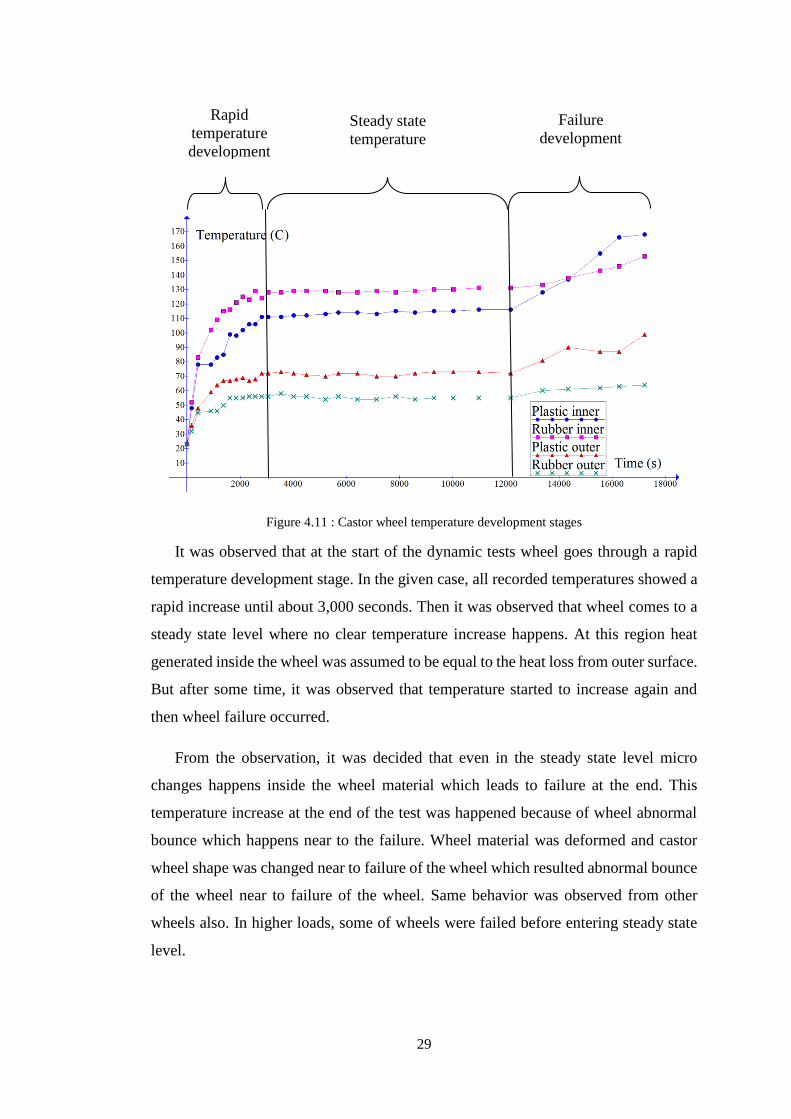
It was observed that at the start of the dynamic tests wheel goes through a rapid
temperature development stage. In the given case, all recorded temperatures showed a
rapid increase until about 3,000 seconds. Then it was observed that wheel comes to a
steady state level where no clear temperature increase happens. At this region heat
generated inside the wheel was assumed to be equal to the heat loss from outer surface.
But after some time, it was observed that temperature started to increase again and
then wheel failure occurred.
From the observation, it was decided that even in the steady state level micro
changes happens inside the wheel material which leads to failure at the end. This
temperature increase at the end of the test was happened because of wheel abnormal
bounce which happens near to the failure. Wheel material was deformed and castor
wheel shape was changed near to failure of the wheel which resulted abnormal bounce
of the wheel near to failure of the wheel. Same behavior was observed from other
wheels also. In higher loads, some of wheels were failed before entering steady state
level.
Rapid
temperature
development
Rapid
temperature
development
Rapid
temperature
development
Rapid
temperature
development
Steady state
temperature
Figure 4.6 :
Castor wheel
temperature
development
stagesSteady
state
temperature
Figure 4.7 :
Castor wheel
temperature
development
stages
Figure 4.8 :
ASTM D638-
Type 1 test
piece
dimensionsFi
gure 4.9 :
Castor wheel
temperature
development
stagesSteady
state
temperature
Figure 4.10 :
Castor wheel
temperature
development
stagesSteady
state
temperature
Failure
development
Failure
development
Failure
development
Failure
development
Figure 4.11 : Castor wheel temperature development stages
Figure 4.12 : ASTM D638-Type 1 test piece dimensionsFigure 4.13 : Castor wheel temperature
development stages
Figure 4.14 : ASTM D638-Type 1 test piece dimensions
Figure 4.15 : Polypropylene Stress-Strain graph at 23oCFigure 4.16 : ASTM D638-Type 1 test
piece dimensionsFigure 4.17 : Castor wheel temperature development stages
Figure 4.18 : ASTM D638-Type 1 test piece dimensionsFigure 4.19 : Castor wheel temperature
development stages

30
4.2. Raw Material Testing
Raw material tests include testing of plastic and rubber materials.
4.2.1. Tensile Test
Uniaxial Tensile test was carried out in rubber, polypropylene and nylon material
to evaluate stress strain behavior of the materials. All the test pieces were made in
house and tested with available tensile test machine Tinius olsen 5ST machine [22].
Plastic material tensile test
Uniaxial tensile test of plastic materials was carried out under ASTM D638
standard. Tensile pieces were made by injection moulding according to standard type
1 dumbbell shape pieces as given is test standard.
Test was carried out in average recommended strain rate of 50mm/minute in
controlled lab temperature of 23oC. strass-Strain graph for the test was extracted from
the tensile machine. This data was used to calculate modulus and yield stress when
giving parameters for the FEA software.
Figure 4.20 : ASTM D638-Type 1 test piece dimensions
Figure 4.21 : Polypropylene Stress-Strain graph at 23oCFigure 4.22 : ASTM
D638-Type 1 test piece dimensions
Figure 4.23 : Polypropylene Stress-Strain graph at 23oC
Figure 4.24 : Nylon Stress-Strain graph at 23ocFigure 4.25 : Polypropylene
Stress-Strain graph at 23oCFigure 4.26 : ASTM D638-Type 1 test piece
dimensions
Figure 4.27 : Polypropylene Stress-Strain graph at 23oCFigure 4.28 : ASTM
D638-Type 1 test piece dimensions
Figure 4.29 : Polypropylene Stress-Strain graph at 23oC
Figure 4.30 : Nylon Stress-Strain graph at 23ocFigure 4.31 : Polypropylene Stress-Strain graph at
23oC
Figure 4.32 : Nylon Stress-Strain graph at 23oc

31
Figure 4.8 shows stress-strain graph of polypropylene material used in castor
wheel. Yield stress of the material is 24.5 MPa according to the obtained graph with
approximately 700% post yield strain.
Figure 4.9 shows Stress strain graph of nylon used for castor wheels. Yield stress
of nylon was 68.4 MPa, which was 2.8 times higher than polypropylene. But nylon
maximum strain was 200%. This higher strength and yield stress was main reason for
use nylon material in heavy load application castor wheels.
Table 4.2 : Plastic material tensile test results
Rubber material tensile test
There were two rubber compounds used in selected castor wheel sample set namely
NR-1 and NR-2. Both those compounds were tested in uniaxial tensile test to get
stress-strain data for each material. ASTM D412 Standard Test Methods for
Vulcanized Rubber and Thermoplastic Elastomers was used as standard to test rubber
materials. Initially compounds were mixed and milled as normal procedure. Then
Units MPa MPa (x100%) (x100%)
Material Modulus Yield Stress Strain at yield Max Strain
PA6 (Nylon) 821.2 68.4 0.083 1.5
PP (Polypropylene) 194.5 24.6 0.126 7.0
Figure 4.36 : Nylon Stress-Strain graph at 23oc

32
rubber 150mmx150mmx2mm rubber sheets was made by compression moulding.
ASTM D412-Type C die was used to cut dumbbell pieces from those moulded sheets.
Standard 200mm/minute speed was used to test those dumb-bell pieces in same
tensile machine. Obtained Stress-Strain graph showed similar behavior and in average
max stress recorded was 15 MPa with about 390% strain. Those graphs were directly
used in FEA software for calculation of material model coefficients. X axis of the
graph represent strain amount of test piece. Y axis shows the stress inside the test piece.
Figure 4.37 : ASTMD 412-Type C rubber specimen dimensions
Figure 4.38 : Rubber Stress-Strain graph at 23oc

33
4.2.2. DMA Test
DMA which is named as dynamic mechanical analyze is mostly used to analyze
viscoelastic behavior of polymers. DMA measures the properties of materials as they
are deformed under periodic sinusoidal stress, which is very similar to behavior of
material when a tyre or castor wheels are rotated under load. Loss modulus and storage
modulus of a viscoelastic material and their variation with temperature can be
extracted by DMA test [23]. The storage modulus represents the stiffness of a
viscoelastic material and is proportional to the energy stored during a loading cycle.
The loss modulus is defined as being proportional to the energy dissipated during one
loading cycle. For example, it represents the energy lost as heat, in a loading cycle of
a viscoelastic material [23].
When castor wheels are rotated under load heat generation happens inside of the
rubber material due to this loss energy because of viscoelastic property of the rubber
material [19]. So only rubber materials were tested in DMA test as it contributes most
of energy for the heat generation inside the wheel.
[24] Various methods are available to test rubber materials in DMA test. ASTM
D5992 Standard Guide for Dynamic Testing of Vulcanized Rubber and Rubber-Like
Materials Using Vibratory Methods was followed when testing rubber in DMA tester.
Rectangular rubber piece 35mmx13.5mmx2.8mm in size, which is cut by
previously described moulded rubber sheet was used as specimen for DMA test. The
test specimen is clamped between the movable and stationary fixtures, and then
enclosed in the thermal chamber. Oscillation frequency and a temperature range
appropriate for the material were given to tester. The Analyzer applies oscillation to
the test sample while slowly moving through the specified temperature range.
Materials were tested for several oscillation frequencies in between -60oC to
+150oC. frequency was selected according to castor wheel rotation speed of 4 km/h
and wheel diameter.
Frequency =Wheel Speed
Wheel Circumference (1)
(1)
(1)

34
Table 4.3 : DMA test oscillation frequency
km/h mm/s mm mm
Wheel Speed Wheel Speed Wheel diameter
wheel circumference Frequency
4 1111.1 80 251.3 4.4
4 1111.1 125 392.7 2.8
4 1111.1 160 502.7 2.2
4 1111.1 180 565.5 2.0
4 1111.1 200 628.3 1.8
It was observed that very similar data curves were given by the DMA test for
various frequencies which suggest this viscoelastic property of the material doesn’t
depend of oscillation frequency. DMA graph for both materials which was done at 2.2
Hz frequency was selected for further studies.
loss modulus and storage modulus was extracted in between given temperature
range -60oc to 150oc as data points from the DMA test machine. Temperate range
selected according to temperatures occurred in castor wheel dynamic testing. As
referenced research paper [9] energy input modulus for the DMA test specimen in each
temperature can be calculated as,
Energy input modulus = √(Storage modulus)2 + (Loss Modulus)2
Then Energy loss fraction of the rubber material at a given temperature can be
calculated as,
Energy loss fraction = Loss modulus
Energy input modulus
Energy loss fraction vs temperature graph was analyzed in both NR-1 and NR-2
rubber compounds and recorded to be used in FEA model creation. Calculated Graphs
are given in Figure 4.12. It was observed in both graphs energy loss fraction started
around 0.08 and went up to 0.2 around -20oC temperature. Then this Energy loss drops
back to0.09 after -15oC and steadily follows similar values after that. in this research
area interest are of the curve was above 23oC which is steady around 0.9-0.8 energy
(2)
(2)
(2)
(2)
(3)
Fig
ure
4.3
9 :
NR
-1
&
NR
-2
En
erg

35
loss fraction. Very similar behavior was observed between NR-1 graph and NR-2
graph.
From energy loss fraction, energy loss at given cycle can be calculated if Total
energy input for the particular cycle is known. These obtained data were checked
against previous researches done on this DMA testing and was fond to be very closely
matching with research data. [9] Yeong-Jyh in his research presented pneumatic tyre
tread rubber material DMA test data which was done at frequencies from 0 Hz to 25
Hz and temperatures from 0oC to 100oC. it was presented that energy loss fraction was
not varied according to variation of frequency. Also from 25oC to 100oC energy loss
fraction was measured as 0.1 in given test which is closely matching with observed
test data.
Figure 4.42 : NR-1 & NR-2 Energy loss fraction vs temperature graphs

36
5. Finite Element Model Development
Finite element analysis (FEA) is well established technology to virtually simulated
real world application and behaviors. When a product is analyzed through FEA for a
loading condition, the setup is broken in to small elements and analyzed in simplified
manner then combined again to give the full results [25].
After castor wheel dynamic tests and raw material testing next step was to develop
finite element simulation model to predict temperature profile of a rotation castor
wheel under load. The simulation models were developed according to Figure 3.1
given in methodology. Initially simulations were done to predict temperature profile
of rotating castor wheel in a given time, the with predicted temperature data simulation
was done to analysis failures of the wheel. To simplify the simulation, 2D plate
simulations were used where ever possible. 160 mm wheel with 450kg load was used
to develop the FEA model as case study.
5.1. Static Loading
Static load simulation of the castor wheel was done to understand stress level of
wheel with given load and to analyze total energy required to load the wheel. For the
simulation, commercially available mid-range FEA software Strand7 [26] was used
with nonlinear static and dynamic analysis capability.
Figure 5.1 : 160 mm Castor wheel dimensions

37
3D FEA analysis was done for the static loading simulation because loading was
done from one location when wheel statically loaded. When considered about this
loading case, it was observed that symmetricity could be considered for this dividing
loading area and 3D model in to ¼ of the model. Figure 5.2 demonstrate the proposed
¼ symmetric model with loading conditions.
Obtained tensile graph of the NR-1 rubber material was loaded in to the software
as a Stress-Strain graph. Tensile graph of nylon was also loaded to the software as
stress-strain graph.
Figure 5.2 : proposed ¼ castor wheel model for FEA
Symmetric plane 1
Symmetric plane 1
Symmetric plane 1
Symmetric plane 1
Symmetric plane 2
Symmetric plane 2
Symmetric plane 2
Symmetric plane 2
Fixed constrain
In bearing surface
Fixed constrain
In bearing surface
Fixed constrain
In bearing surface
Fixed constrain
In bearing surface
¼ of original load
Applied from bottom
Figure 5.2 : proposed
¼ castor wheel
model for FEA¼ of
original load
Applied from bottom
Figure 5.3 : proposed ¼
castor wheel model for
FEA
¼ of original load
Applied from bottom
Figure 5.4 : proposed
¼ castor wheel
model for FEA¼ of
original load

38
5.1.1. Mesh Creation
when considered about required 3D model mesh, several element types are
available as given in Figure 5.3 to mesh a model and do analysis. Element type was
selected according to literature of rubber and plastic product simulations. Mostly 20
node hexahedrons were used in 3D simulations and 8 node plate elements were used
in 2D simulations in literature to simulate filled rubber components and plastic
components because of results accuracy and efficiency. Same element type was used
in this research also [26] [27]. Element size of the mesh was selected after several
analyses done by possible element size and developing a convergence graph. Initially
½ of 2D profile of the wheel was imported to FEA software. Then according to selected
element size 2D profile was meshed with 8 node plate elements and revolved to form
20 node hexahedron elements in 3D mesh.
Convergence plot was developed to select the best element size for the simulation.
Model was simulated in various element sizes and maximum stress developed in the
plastic region of the model for given load was recorded and plotted.
Stress in the plastic region was selected because rubber region stress was much
lower value than plastic region. Mesh size was defined as percentage for the maximum
dimension in the model so when wheel size changed accordingly proper mesh size can
be derived from percentage.
Figure 5.3 : FEA Elements available for 3D simulation

39
Table 5.1 : Max stress in plastic vs Element size
mm kg MPa 2D
Element size
Element size for 160 mm
wheel Wheel load
Max Stress in plastic
9.0% 14.4 450 17.50
8.0% 12.8 450 19.50
7.0% 11.2 450 20.10
6.0% 9.6 450 20.50
5.0% 8.0 450 20.63
4.0% 6.4 450 20.64
3.0% 4.8 450 20.65
2.0% 3.2 450 20.66
From Figure 5.4 it was observed that before 5% element size graph converge to a
stable value. for Castor wheel 2D profile 8 node plate elements were created in the size
of 5% from maximum dimension of the castor wheel model. Then they were revolved
around wheel axis initially by 2 degrees until 30 digress, and the by 6 degrees until
180 degrees. Initial 2 degrees were created more densely to be used in contact analysis.
the Same element size percentage was selected to mesh the models of all the wheels.
Figure 5.4: Convergence analyze for selecting mesh size

40
5.1.2. Boundary Conditions
Fixed boundary condition for the bearing area was applied as model is supported
by bearings. In the 3D model bearings were not modeled, boundary conditions were
applied to the plastic center bearing area directly to simplify the simulation. Bearing
effect was not considered in simulations.
Symmetric boundary conditions for both symmetric planes were applied as next
step. Separate boundary conditions were defined for fixed location and two symmetric
planes where castor wheel was split to simplify the FEA model.
Figure 5.5 : Meshed 3D model of 160 mm Castor wheel
Symmetric
Constrains
Symmetric
Constrains
Symmetric
Constrains
Symmetric
Constrains
Fixed
constrains
Figure 5.8 :
Meshed model
with boundary
conditionsFixe
d constrains
Figure 5.9 :
Meshed model
with boundary
conditions
Fixed
constrains
Figure 5.6 : Meshed model with boundary conditions
High density mesh for
contact area with floor
Figure 5.5 : Meshed
3D model of 160 mm
Castor wheelHigh
density mesh for
contact area with floor
Figure 5.6 : Meshed 3D
model of 160 mm Castor
wheel
High density mesh for
contact area with floor
Figure 5.7 : Meshed
3D model of 160 mm
Castor wheelHigh
density mesh for
contact area with floor

41
Load was applied on the castor wheel as compression force which applied through
floor. Initially contact between castor wheel and floor was defined by contact element.
Strand7 software use “node to node” contact method to define contact between two
bodies. Other advance contact definitions are “surface to node” and “surface to
surface” which needs higher computational power and generally used with complex
contact problems. In the castor wheel simulation floor to wheel contact is
straightforward and “node to node” contact definition is the most effective contact
definition to be used here [26], [28].
From 3D mesh approximately contact area of the rubber wheel was selected and
nodes in that area were extruded to form floor nodes with beam elements. The point
contact definition was used to define those beams, so when beam length becomes 0 it
acts as contacted node.
Then all those floor nodes were connected with rigid beams to form a one cluster
node. Cluster node was given constrain to move upwards along with the floor until
floor compresses rubber wheel generation a reaction force on the cluster node. From
the reaction on the cluster node load acted on the wheel was calculated to a given wheel
compression.
Contact element parameters were selected as standard parameters and kept as fixed
values throughout case study models to maintain uniformity.
Beam
elements
Defined floor at end of beams
Cluster nodes
With rigid connections
Figure 5.7 : FEA model with loading conditions

42
FEA Material models for plastic and rubber materials
Elastic
Isotropic
Orthotropic
Anisotropic
Elasto-Plastic
Isotropic
Orthotropic
Anisotropic
Hyperelastic
Fung
Mooney–Rivlin
Ogden
Polynomial
Saint Venant–Kirchhoff
Viscoelastic
Temperature effects
Hysteresis
Rubber Damage models
Creep / Stress Relaxation
5.1.3. Material Models
Lots of material models are available in FEA to various types of materials and
behaviors. For plastic materials, separate material model was defined and for rubber
material separate material model was defined in the FEA software. All the elements
belong to plastic category was assigned with plastic material model and all the
elements belong to rubber material was assigned with rubber material model.
Material models related to plastic and rubber in FEA can be divided in to four main
categories namely elastic, elastic-plastic, hyperelastic and viscoelastic. Apart from
this, various other material models also available to define different types of materials.
for example, sand or water behavior modeling in FEA is done in their own material
models. Elastic-Plastic material model is an extension of Elastic model to plastic
region.
Figure 5.8 : Material models used in FEA

43
Plastic material model was selected as Elastic-Plastic Isotropic material model
according to plastic material behavior. Generally, plastics are defined as isotropic
material which means physical property has the same behavior when measured in
different directions. Initial linear elastic region and after yielding plastic deformation
region was observed in tensile graphs of both polypropylene and nylon which qualify
them for Elastic-Plastic behavior. Both polypropylene and nylon materials were
defined as Isotropic Elastic-Plastic material model. For 160 mm wheel simulation,
previously loaded tensile graph of nylon was assigned to defined material models
inside the software along with relevant elements.
Selection of appropriate material model for rubber material was done considering
literature data provided in previous research works done. Both hyperelastic and
viscoelastic material can be used in modelling rubber material.
Viscoelastic material models are advanced material models which can simulate
time, temperature dependency of rubber material. Those models incorporate
Hysteresis effects, rubber damage, creep and stress relaxation effects of rubber
material. Complex material property analysis relevant to each and every application,
need to done to define those material models in FEA and get accurate results. Very
high computation power also required to solve these material models.
Hyperelastic material models are relatively simple material models for rubber
material. These models are time independent models which means separate methods
need to follow if those types of simulations are needed with hyperelastic models.
Material models can be defied with simple tensile test and require less computational
power to solve and get accurate results.
Generalized Mooney-Rivlin material model under hyperelastic category was
selected to model rubber material in castor wheel simulation based on successful
literature [7] [9]. This material model was recommended by Strand7 software supplier
also for filled rubber product simulation. Mooney-Rivlin constants which are needed
to define the material model, were calculated from the provided tool in Strand7
software directly from loaded rubber tensile graph.

44
5.1.4. Solver Setup
Developed castor wheel was used with nonlinear static solver. Nonlinear solver
was used because of nonlinear behavior of rubber material, high strain levels in rubber
and contact element definitions in the FEA model which violates linear solver
limitations. For the static loading case, Nonlinear Static solver was selected.
Solver parameters can be defined to break the full analysis to small fractions. When
defined, solver solves each fraction of the analysis at a time to evaluated and capture
the nonlinear behavior of the simulation model. In the study fractions were defined as
floor compression movement in to the wheel. Defined floor was compressed in to the
castor wheel by 5mm through solver in 50 steps. 5mm was divided to equal 50
fractions of 0.1mm and solver pushed the floor up by 0.1mm in each step. Since rubber
wheel was fixed from center, when floor was pushed in to the rubber generated a
reaction force on floor which is equivalent to wheel load at given solver step. Iterative
solving was done for each step until forces and resultant displacements in FEA model
gets to equilibrium and stabilized. Then again solver goes to next step. In each step,
all the calculations for stress build up, reaction force, node shape change were done
and recorded in results file as 50 steps.
5.1.5. Simulation Results
Reaction force on the cluster node in each step was extracted from results file to
find the step which 450 kg load was applied to the castor wheel. Since ¼ of the model
was used in the simulation reaction equivalent to ¼ of 450 kg would give the relevant
step.
Case study load on wheel = 450 kg
Equivalent Force = 450x9.81
= 4414.5 N
Because ¼ of the model is used in FEA simulation,
Relevant FEA model reaction = 4414.5 / 4
= 1,104 N

45
It was observed that solver step relevant to 450 kg wheel load is 39th step from the
given graph. At the given 39th step stress inside the wheel was analyzed. To define the
stress inside the rubber and plastic material von Mises definition was used. This given
stress can be directly compared with plastic yield stress for yielding or safety factors
using von Mises yield criterion [29]. Reaction force vs wheel compression graph was
observed to get the wheel compression which was 3.9 mm at given wheel load of 450
kg.
Figure 5.9 : Reaction force vs Solver step graph of 160 mm wheel
Figure 5.10 : Reaction force vs Wheel compression of 160 mm wheel

46
Display colour Level
High
Mid
Low
Stress distribution of the wheel was observed at load 450 kg and found close
relation for the wheel failures at dynamic test. Highest von Mises stress was recorded
in plastic center in the area were wheel fails at dynamic load.
Figure 5.11 : von Mises stress distribution of 160 mm wheel
Figure 5.13 : Stress in Plastic 160 mm
wheel (Original in colour) Figure 5.12 : Stress in rubber 160 mm
wheel (Original in colour)
High stress area
marked in red
Figure 5.14 : von
Mises stress
distribution of 160
mm wheelHigh
stress area marked
in red
Figure 5.15 : von Mises
stress distribution of
160 mm wheel
High stress area
marked in red
Figure 5.16 : von
Mises stress
distribution of 160
mm wheelHigh
stress area marked
in red

47
Stress developed in castor wheel for 450 kg static loading given in table.
Table 5.2 : 160 mm wheel, 450 kg static load safety factor
MPa MPa MPa MPa
load Stress in
nylon centre
Stress in NR-1
rubber
Nylon yield stress
NR-1 max stress
Safety factor for
nylon centre
Safety factor for
rubber wheel
450 kg 20.6 6.9 68.4 15.0 3.3 2.2
3.3 safety factor was observed for the Nylon center of the 160 mm wheel for 450
kg load. 2.2 safety factor was observed from the rubber wheel for 450 kg load in static
loading condition.
5.2. Total Energy Rate Calculation
Total energy rate inside the rubber when castor wheel was rotated under load was
calculated for 160 mm wheel 450 kg dynamic test simulation. This was done by
combining static load simulation results and DMA test results.
Initially total energy given to the wheel when wheel was statically loaded to 450kg
was calculated. Wheel reaction load vs Wheel compression graph given in Figure 5.10
was extracted from the static FEA simulation data and used to calculate total energy
input to the system. 3.9mm compression was observed from the graph when wheel
was loaded with 450 kg. Area under graph was calculated from x=0 to x=3.9mm to get
total energy input to the system to load wheel up to 450 kg load. To calculate the area
under the curve Riemann sum method with right boundary rectangle approximation
was used. Graph was divided in to small rectangles with 0.1mm “x” width and height
of “y” value where right boundary of rectangle touching the graph [30].
Then area of all these rectangles was sum to get area under the curve. Figure 5.10
Graph shows reaction force from developed ¼ model, so given force was multiplied
by 4 in each step to get actual force to load full castor wheel.

48
From appendix 2:
Total energy input to static loading at 450kg load = 6.3 J
Then static energy was converted to energy input to the system in one second when
wheel was rotated under 450 kg load at 4 km/h speed, which is called as total energy
rate
Total Energy rate
= 6.3 x Number of wheel rotations in one second x correction factor
Number of wheel rotations in one second calculation,
Wheel rotation speed = 4 km/h
Wheel rotation speed = 1111.1 mm/s
Wheel diameter = 160 mm
Wheel perimeter = 160 x Pi
= 502.65 mm
Number of wheel rotations per second = 1,111.1 / 502.6
= 2.2
Correction factor calculation,
Correction factor was introduced in this calculation to convert static loading
energy to steady state rolling energy. Initially correction factor was set to 1 and
modeling was continued till castor wheel temperature prediction model. Then rubber
inner temperature was compared in prediction model and actual. In actual heat inside
the rubber at Steady state was recorded as 131oC. then with trial and error method
correct factor was selected. This factor was used as fixed factor for other validation
models.
Table 5.3 : Correction factor calculation
Correction factor Actual temperature oC Predicted temperature oC
1 131 90
2 131 110
3 131 120
3.1 131 126
3.2 131 130 3.25 131 131
(4)
(4)
(4)
(4)
(5)
(5)
(5)
(5)

49
Selected correction factor = 3.25
Total energy rate for 450 kg loaded rotating wheel in one second, From equation (5)
Total Energy rate = 6.3 x 2.2 x 3.25 J/s
= 45.25 J/s
Total energy rate is the energy absorbed by castor wheel in one second when
wheel is rotated under 450 kg load. Due to viscoelastic behavior of the rubber part of
this energy is converted in to heat energy. This loss energy was calculated by
combining DMA test data with total energy rate.
In Figure 4.12 graph shows rubber materials energy loss fraction against
temperature in cyclic loading. Hence to get energy converted to heat energy by rubber
wheel in one second heat generation rate was defined,
Heat generation rate = Total energy rate x Energy loss fraction
Heat generation rate inside the rubber was calculated from equation 6. It was
assumed that total energy given to the system is totally absorbed by rubber and energy
absorbed by plastic is negligible.
5.3. Temperature Prediction
A FEA model to predict castor wheel developed temperature profile after a given
time of dynamic test was developed. 2D axisymmetric FEA model was used to this
temperature profile prediction model. Computational cost of model is reduce because
of the use of this axisymmetric model.
In this model wheel was modeled as 2D profile and input was given to software to
consider as axisymmetric along a selected wheel center line axis, which means
software assumes the model as revolved profile. 8 node 2D plate elements were used
with 5% selected element size to mesh the model. 2D simulations are very effective
simulation which takes very less time to solve and give accurate results.
(6)
(6)
(6)
(6)

50
5.3.1. 2D Model and Mesh Creation
2D profile of castor wheel was imported to the software then meshing was done
according to 5% mesh sizes to elements sizes to be identical with 3D mesh. Then
axisymmetric boundary conditions and symmetric boundary conditions were applied
to the developed mesh.
5.3.2. Heat Generation Rate
Previously calculated total energy rate was used as heat source inside the rubber
wheel for the thermal simulation. To distribute the total energy rate among 2D model
rubber elements, stored energy of rubber element in the 3D static 450 kg loading case
was used.
According to the stored energy in static loading case surface elements, total energy
rate was distributed among initial 75% of the elements. Each element storage energy
was calculated ad divided by total energy to get relevant distribution factor. Distributed
total energy rate was applied as heat sources at each rubber element. Calculation is
given in Appendix three.
Figure 5.14 : 2D axisymmetric model
Axisymmetric Axis
Axisymmetric Axis
Axisymmetric Axis
Axisymmetric Axis
Symmetric edge
constrains
Figure 5.17 : 2D
axisymmetric
modelSymmetric
edge constrains
Figure 5.18 : 2D
axisymmetric model
Symmetric edge
constrains
Figure 5.19 : 2D
axisymmetric
modelSymmetric
edge constrains

51
Table 5.4 : Total energy rate distribution
j/s Element
ID Total energy
rate
136 4.27
121 4.13
586 2.98
676 2.91
106 2.68
151 2.60
391 2.43
601 2.24
376 2.02
406 1.89
616 1.85
46 1.85
421 1.68
706 1.67
451 1.62
571 1.61
61 1.52
646 1.40
556 1.36
241 1.28
31 1.24
Figure 5.15 : 2D profile with heat sources applied to relevant elements
Applied heat
sources in red dots
Figure 5.20 : 2D
profile with heat
sources applied to
relevant
elementsApplied
heat sources in red
dots

52
From total energy rate, heat generation rate should be calculated as,
Heat generation rate = Total energy rate x Energy loss fraction
Energy loss fraction graph according to the Figure 4.12 was loaded in to the
software and instructions were loaded to software to calculate the heat generation rate
accordingly in each calculation according to part temperature. Energy loss fraction was
calculated from rubber material DMA tests according to proven literature. This graph
can be varied according to temperature also according to the details fed in to software.
Heat generation rate was controlled according to time also since castor wheel
dynamic test was carried out as 3-minute run and 1 minute stop. At one minute stop
time, heat generation rate should be zero inside the rubber.
To achieve this another table was defined in the FEA software and wheel run cycle
was loaded as given in Figure 5.16. Calculated heat generation rate was multiplied by
1, in first 3 minutes and in next minute it was multiplied by 0. This cycle was continued
until 300 minutes which is more than maximum wheel run time.
Figure 5.16 : Castor wheel run cycle graph
(7)
Fig
ure
5.2
3 :
Cas
tor
wh
eel
run
cyc
le
gra
ph(
7)
Figu
re
5.24
:
Cast
or
whe
el
run
cycl
e
grap
h
(7)
Fig
ure
5.2
5 :
Cas
tor
wh

53
5.3.3. Thermal boundary conditions
Thermal boundary conditions for the castor wheel model which includes heat
capacity, heat conductivity of materials, convection heat loss from surface was loaded
to the software next. These data were needed to define the proper simulation model. It
was assumed that these data do not change with time or temperature during the course
of simulation.
Data was extracted from literature data where FEA thermal simulations were done
with success [9] [18]. Mass density of rubber and plastic was measured by in-house
specific gravity tester and calculated accordingly. Each material data was assigned to
relevant rubber and plastic elements through the software. Surface heat convection
coefficient and initial temperatures of the model was also allocated to relevant
elements and element surfaces.
Table 5.5 : Material properties for thermal simulation
Material Mass
Density Specific Heat
capacity Heat
conductivity Forced
Convection-Air
Rubber to floor
kg/mm3 W/kg/k W/mm/c W/mm2/ c ◦ W/mm2/ c ◦
PP 9.1x10⁻⁷ 1800 1.8x10⁻⁴ 6 x10⁻⁶
Nylon 1.25x10⁻⁶ 1700 2.6 x10⁻⁴ 6 x10⁻⁶
NR-1 1.210-6 1700 2.39 x10⁻⁴ 6 x10⁻⁶ 1 x10⁻⁴
NR-2 1.2x10⁻⁶ 1700 2.39 x10⁻⁴ 6 x10⁻⁶ 1 x10⁻⁴
5.3.4. Solver setup
Transient heat solver was used to simulate the developed model with 1 second
intervals until 10,000 seconds which equals to dynamic test time of 160 mm wheel
under 450 kg load. Each second solver solves the equations and record temperatures
and other property data.
Then according to the developed temperatures next solving was done. This
simulation was a very accurate and efficient simulation because the use of 2D
simulation.

54
5.3.5. Simulation results
Temperature development inside the castor wheel in previously defined
temperature measuring points was analyzed from the model. In each measuring point
how temperature increases with the time was plotted in graph through the software.
It was observed from the graph that temperature raise and drops cyclic manner
relative to wheel run and stop time. But this behavior was not prominent in plastic
outer location. Max temperature recorded was observed and rubber inner temperature
was the highest recorded in the simulation which went up to 131oC. Then plastic outer
Figure 5.17: Temperature extracted points from 2D simulation
Figure 5.18 : 160 mm 450 kg FEA simulation temperature prediction

55
Display colour Level
High
Mid
Low
recorded a temperature at 115oC before plastic inner temperature of 76oC. Lowest
temperature of 53oC was recorded at rubber outer where higher convection rate was
defined because rubber touches the floor.
Also from the graph we could see that temperature development in the castor
comes to a steady state level roughly after about 3,200 seconds when run stop behavior
was neglected. For the simulation results steady state was defined as when temperature
difference is less than 0.5oC in adjust temperature points just after wheel enter stop
cycle. This temperature distribution after 3,200 seconds, maximum temperature
recorded given in Figure 5.19. It was observed that in actual dynamic test also wheel
attain this steady state level. Then after some time temperature starts to go up again
because of abnormal bouncing of the wheel which generate higher amount of heat than
normal rotation.
Figure 5.19 : Steady state max temperature profile, 160 mm 450 kg
131oC
Figure
5.26 :
Steady
state
max
temper
ature
profile,
160
mm
115oC
115oC
115oC
115oC
77oC
77oC
77oC
77oC
53oC
53oC
53oC
53oC

56
Temperature profile of maximum temperature attained by the simulation was
analyzed. Profile exhibits the same values as measured temperatures from the actual
dynamic test. There was no clear region between plastic and rubber boundaries
because of close thermal material properties of rubber and plastic.
Also, it was observed that center area of the wheel which connects to bearing, was
heated to very low temperature because of effective length from heat generation area
and surface convection of developed heat, heat transferred to that area was low.
Temperature graphs obtained from the prediction was compared with actual
results. From equation 5 correction factor was calculated based on rubber inner
temperature only, so other temperature components were compared with predicted
temperature values to observe validity of the calculated correction factor.
In actual for 17,000 s wheel continued dynamic test, but from Figure 5.18 graphs
it was observed that steady state level was achieved after about 3,200 s.
Steady state rubber inner temperature was selected to tune the FEA temperature
prediction model which was the reason for very close matching of the comparison.
Tuning was done only for first case study. This was used as fixed number for the rest
of simulations.
Figure 5.20 : Rubber inner temperature comparison, 160 mm 450 kg

57
It was observed that steady state temperatures of actual and predicted plastic inner
Figures also very close to each other. But in actual after 13,500 s it was observed that
center temperature was increased further. In most of test results this temperature raise
was observed when wheel was close to failure, abnormal bouncing of the wheel close
to failure was the reason for this which was not captured in this simulation model.
Figure 5.21 : Plastic inner temperature comparison, 160 mm 450 kg
Figure 5.22 : Plastic outer temperature comparison, 160 mm 450 kg

58
Both plastic outer and rubber outer temperatures also found to be closely prediction
actual steady state temperatures. For temperature comparison observations 3.25
correction factor calculated in equation 5 was validated.
5.4. Failure Analysis
Failure was observed from the center part of the wheel in actual dynamic
simulation. So, the failure analysis was focused on detecting center part failures
through FEA simulation when wheel was heated by hysteresis energy loss from the
rubber. Temperature, applied load and material property changes with temperature
mainly contributes for center plastic failure. When wheels are rotated under load they
achieve steady state temperature level and then after some time temperature starts to
raise again close to wheel failure due to yielding and bouncing of wheel. This final
failure mechanical involves very complex physical behavior which was very complex
to solve in general FEA application. It was observed that wheels at lighter loads
continued on dynamic test longer than wheels at higher loads which failed sooner in
dynamic test. Failure analysis was done to identify wheel failures at steady state level,
if wheel was identified as failed at steady stated level it would fail in dynamic test
sooner, if wheel was identified as not failed at steady state level, it would continue
longer time at steady state level on dynamic test before actual failure.
Figure 5.23 : Rubber outer temperature comparison, 160 mm 450 kg

59
A 2D axisymmetric model was developed to analyze those effects and identify
failures at steady state level. Use of 2D analysis was effective at this stage as
temperature prediction was also done as 2D axisymmetric simulation. 2D model solver
treats loads are applied all around the wheel, unlike 3D static load simulation. It was
required to calculate the equivalent load on 2D static model to stress the center part to
same level as 3D static model at 450kg load.
5.4.1. Equivalent Load Calculation
Same 2D profile as Figure 5.14 was used for this simulation. Meshing of the model
was done according to 5% of maximum model dimension which gives same mesh as
thermal simulation. Material properties and boundary conditions were loaded as 3D
static loading case for this axisymmetric 2D model. Beam elements were modeled as
point contact elements and floor was defined at the end. For the beam contact
parameters, same parameters were used as 3D static loading model. Nonlinear static
solver was used to push the floor in to the rubber by 5mm generating reaction force on
cluster node. Initially maximum stress developed in the center was analyzed and solver
increment was identified which gives same stress in center as 3D static simulation
result. For the solver step, reaction force was recorded which gives same stress. It was
assumed that in those both cases, 3D static simulation with 450 kg load, 2D
axisymmetric simulation with recorded reaction force, Loads and stress acting in the
center part of the wheel was same. So, comparison can be done and predictions can be
done about 3D behavior of the wheel under 45 0kg load, from developed 2D model
under recorded reaction force.
Plate elements – Plastic
material
Plate elements – Plastic
material
Plate elements – Plastic
material
Plate elements – Plastic
material
Plate elements – Rubber
material
Plate elements – Rubber
material
Plate elements – Rubber
material
Plate elements – Rubber
material
Symmetric constrains
Symmetric constrains
Symmetric constrains
Symmetric constrains
Beam elements - Contact
Beam elements - Contact
Beam elements - Contact
Beam elements - Contact
Rigid Links
Figure 5.31 : 160mm castor
wheel 2D profileRigid Links
Figure 5.32 : 160mm castor wheel
2D profile
Figure 5.33 : 160 mm wheel
Cluster node
Cluster node
Cluster node
Cluster node
Figure 5.24 : 160 mm castor wheel 2D profile

60
In the 3D static load simulation, it was observed that center was stressed up to
20.3 MPa at 450kg load as given in table 6. In the 2D simulation same stress level of
20.3 MPa was developed in the center part at 28th solver increment. This increment
was selected by analyzing Stress profiles and Stress levels of each increment given by
the software.
Figure 5.25 : 160 mm wheel 2D profile stress distortion
Figure 5.26 : Reaction force on cluster node vs Solver increment

61
From the Figure 5.26 reaction force at increment 28 was observed as 3,814 N. for
the 160 mm wheel 450 kg loading case we can define equivalent load as,
2D 450 kg static loading Equivalent load = 3814 N on cluster for 2D simulation
From other way, when 2D model was loaded up to 3,814 N load to the cluster node,
behavior inside the center would be equal to static 3D model 450 kg loading case
behavior. Analyzing of the 2D profile was very fast and effective way to evaluate stress
development in the wheel loading.
5.4.2. 2D simulation Model with Temperature Effects
After calculation of equivalent load, same 2D model was used to simulate the
loading case with temperature effects. Material tensile graph which were loaded as
fixed property graphs where changed to variable property graphs according to material
temperature. Then again 2D static simulation was done to observed stress
development. In the model solver increment, which was loaded to 3,814 N at cluster
node was analyzed to obtain relevant stress levels.
Tensile properties of plastic were tested in elevated temperatures to obtain modulus
and yield Stress in relevant temperature and analyze effect of temperature to material
properties. These results were compared with material data sheets, literature data and
validated for the final results [31]. Those results were summarized in to a table to be
loaded in to the FEA software directly. Table 10 & 11 summarized the results obtained
from testing and literature.
Table 5.6 : Nylon Tensile data variation with temperature
For nylon material, tensile test 23oC gave 82.21 MPa modulus and 68.4 MPa yield
stress. It was observed that at 140oC these values were reduced to 614 MPa and 19.9
MPa respectively. Since these values indicated the strength of the material it was
observed that strength of the material reduced with increased temperature. Between
Temperature (oC) Modulus(MPa) Yield (MPa)
23 821.2 68.4
140 614.0 19.9

62
those temperature values 23oc and 140oc it was assumed that material property changes
were linear.
Table 5.7 : Polypropylene Tensile data variation with temperature
194.5 MPa modulus and 24.6 MPa yield stress was observed for polypropylene
tensile results at 23oC. those parameters were reduced to 152 MPa and 9.2 MPa
respectively at 120oC elevated temperature tensile testing.
Recorded nylon material properties were loaded in to the FEA software for
loading simulation with temperature.
Steady state region maximum temperature profile of 2D temperature simulation of
160 mm wheel at 450 kg load was directly imported as fixed temperatures at nodes.
Since both models have same elements and mesh, it was possible and easy to import
temperatures from previous simulations. These temperatures we imported as separate
loading case for the 2D model then from the solver temperatures were applied before
loading of the model.
Temperature (oC) Modulus(MPa) Yield (MPa)
23 194.5 24.6
120 152.0 9.2
Figure 5.27 : Applied temperature profile, 160 mm wheel, 450 kg loading
131oC
Figure
5.45 :
Applie
d
temper
ature
115oC
115oC
115oC
115oC
77oC
77oC
77oC
77oC
53oC
53oC
53oC

63
5.4.3. Simulation results
Nonlinear static solver was used with temperature effects enabled to simulate the
given models and obtain results. Initially given temperatures were loaded to the nods
before applying the loads. Then floor was pushed in to the rubber wheel by 5mm to
generate reaction load on cluster note where wheel loading was calculated. From the
results reaction load on cluster node vs Solver step graph was obtained and analyzed.
Solver step which applies 3,814 N load on cluster node was identified from the graph.
3,814 N was the calculated equivalent load for 160 mm wheel 450 kg loading case, so
at this identified solver step stress development inside the center would give an idea
about 3D loading condition. At this step stress inside the center was analyzed to study
yielding of the center part to detect failures.
Initial 20 steps in the solver was used to apply the temperature gradually from 230c
to defined temperature profile. Hence reaction force on cluster node was 0 on these
steps. Floor was pushed in to the rubber and load was applied from 21st to 70th solver
steps where reaction force on cluster node was developed. It was observed that 3,814
Figure 5.28 : Reaction force vs Solver step for temperature effect simulation

64
N was developed in cluster node at 49th increment of the solver. Stress developed
inside the center was observed in selected 49th increment.
Table 5.8 : 160 mm 450 kg wheel safety factor
Maximum of 20.5 MPa von Mises stress was observed inside the center part of
the wheel. According to von Mises criteria this stress can be compared with yield stress
of the material to find failure locations of the wheel. It was defined that if Developed
stress exceeds Yield stress of the material it would yield and cause possible failures.
Since this analysis was done in elevated temperature stress at give point should be
compared with material properties of the given point temperature.
Highest temperature of 118oC inside the center was recorded in the same place
where highest stress was recorded according to Figure 5.29. Since same place recorded
MPa MPa
Equivalent load
Stress in nylon centre
Nylon yield stress at
118oC
Safety factor
for nylon centre
450 kg 20.5 29.0 1.41
Figure 5.29 : 160 mm castor 450 kg stress profile

65
highest stress and highest temperature same location was the lowest safety factor
location. safety factor was compared between given location yield stress according to
temperature and observed 20.5 MPa von Mises stress.
1.41 Safety factor was observed in steady state level of the castor wheel which
suggest wheel would run on dynamic test for a longer time. Form physical test data
also it was observed that wheel ran total of 17,220 seconds until it fails (Appendix 1).
Actual standard requirement was to run wheel up to 9048 seconds which suggest wheel
passed the test in physical test. From safety factor analysis also, castor wheel was
marked as pass as it achieved more than 1 safety factor at steady state level.
Steady state was achieved by the castor wheel after 3,200 seconds, so between
3,200 seconds and 17,220 seconds wheel was running with 1.41 safety factor. While
running of the wheel this safety factor might be lowered gradually due to complex
material behavior under dynamic load to fail the wheel at 17,220 seconds.

66
5.5. Generalized model
From case study data and material tests used, Generalized FEA model was
developed to simulate castor wheel designs to evaluate castor wheel dynamic test
performance. Steps done in the given study was summarized and developed to be
followed when new design evaluations are to be done. Given steps describes the
generalized model steps one by one,
• 2D profile of the castor wheel new design should be developed and should be
simplified considering symmetry.
o 2D profile should be ½ of axisymmetric model if symmetrical
• Developed models should exported as IEGS, STEP format to import in to FEA
software
• Materials used for the center part and rubber should be selected
• Raw material testing to be carried out to test center material and collect
material parameters or get data from Appendix 4 / Material data sheets
o Uni-axial tensile test 23oc
o Uni-axial tensile test in elevated temperature 120oC,140oC
o Poison ratio
o Material density
o Heat conductivity
Figure 5.30 : Example models for 2D profile
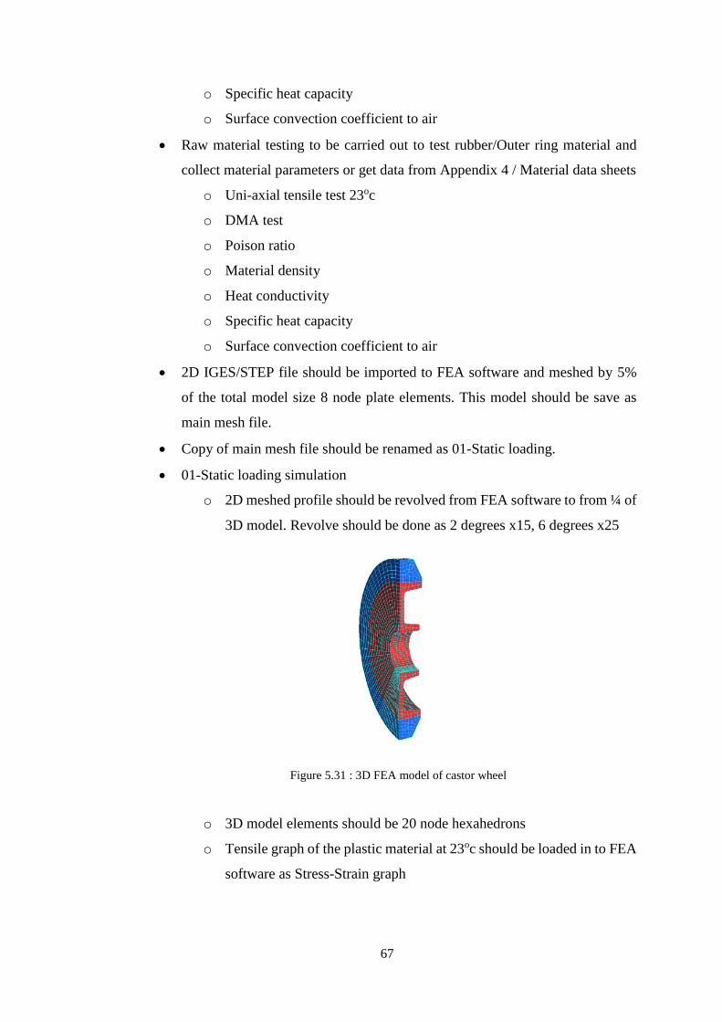
67
o Specific heat capacity
o Surface convection coefficient to air
• Raw material testing to be carried out to test rubber/Outer ring material and
collect material parameters or get data from Appendix 4 / Material data sheets
o Uni-axial tensile test 23oc
o DMA test
o Poison ratio
o Material density
o Heat conductivity
o Specific heat capacity
o Surface convection coefficient to air
• 2D IGES/STEP file should be imported to FEA software and meshed by 5%
of the total model size 8 node plate elements. This model should be save as
main mesh file.
• Copy of main mesh file should be renamed as 01-Static loading.
• 01-Static loading simulation
o 2D meshed profile should be revolved from FEA software to from ¼ of
3D model. Revolve should be done as 2 degrees x15, 6 degrees x25
o 3D model elements should be 20 node hexahedrons
o Tensile graph of the plastic material at 23oc should be loaded in to FEA
software as Stress-Strain graph
Figure 5.31 : 3D FEA model of castor wheel

68
o Center part elements should be selected and assigned with Elasto-
Plastic material model with loaded tensile graph
o Tensile graph of the rubber material should be loaded in to FEA
software as Stress-Strain graph
o Outer ring part elements should be selected and assigned with rubber
material model Mooney-Revlin.
o Tensile graph of rubber material should be assigned to Mooney-Revlin
material model to calculate coefficients automatically
o Fixed constrains and symmetric surface constrains should be applied to
relevant nodes in relevant planes
o Beam elements should be created from outer ring approximate contact
area to form floor
o Bean element should be defined as point contact elements
o End of those beam elements should be connected to one node called
cluster node which compresses the rubber wheel by 5 mm in
simulation.
o Nonlinear static solver should be used to solve the defined FEA model
Figure 5.32 : 3D FEA model with beam and cluster node at bottom

69
o Reaction force on cluster node vs Solver step graph should be obtained
and step should be identified which applies given load for the wheel
considering symmetry
o At given step von mises stress inside the rubber and plastic can be
compared with material yield stress to identify static safety-factor
• 02-Total energy rate calculation
o From 01-static load simulation Reaction force vs rubber ring
compression graph should be obtained
o Integration to be used to calculated the area under the defined graph up
to identified solver step in previous simulation for given load
o Integration results give the energy spent to compress wheel under
given load in static loading.
o This can be assumed as energy absorbed to rubber ring
o From this static energy calculation, should be done to obtain the energy
absorbed by rubber ring to one rotation in dynamic loading.
o Total Energy rate =
Static energy x Number of wheel rotations in one second x correction factor
o Number of wheel rotations per one second was calculated according to
dynamic test speed and wheel diameter
o Calculated correction factor = 3.25
o Form equation total energy rate should be obtained to be used in
temperature prediction FEA model
o From rubber material DMA test data energy loss fraction vs
temperature graph should be obtained
▪ DMA test gives storage modulus and loss modulus of material
and their variation according to temperature
▪ Energy input modulus = √(Storage modulus)2 + (Loss Modulus)2
▪ Energy loss fraction = Loss modulus
Energy input modulus
▪ From given equations energy loss fraction can be calculated and
graph according to temperature
• 03-Tempreature profile prediction model

70
o Copy of main mesh file to be renamed as 03-Tempreature prediction
model
o Calculated total energy rate should be distributed to relevant rubber
elements to represent their heat generation when dynamic test
o From 3D static simulation model relevant surface rubber elements were
selected and from FEA software stored energy density in elements and
element volumes should be extracted.
o Then from that data energy stored in elements should be calculated to
static loading case.
o First 75% of the elements should be selected and among them which
has maximum stored energy
o Calculated total energy rate should be distrusted according to
calculated stored energy among those elements in 2D temperature
simulation model as heat sources.
o Energy loss fraction graph from DMA test should be loaded in to
software and assigned total energy rate should be multiplied by loss
energy fraction to obtain heat generation rate in a given temperature
o Material thermal properties tested or extracted from Appendix 4 should
be loaded in to the software
o Convection coefficients should be assigned to relevant surface edges
with initial temperature
Figure 5.3350 : Temperature prediction 2D model with heat sources

71
o Transient heat solver should be used with time step of 1s up to 10,000s
to analyze the temperature development inside the wheel
o Nodes should be selected to represent rubber inner, rubber outer, plastic
inner, plastic outer and temperature vs time graph should be obtained
to observed temperature development.
o Time till wheel comes to steady state should be identified
o Temperature at steady stated should be identified
• 04-Wheel failure analysis
o Copy of main mesh file should be renamed as 04-faliure analysis-1
o As 3D static loading simulation material properties, contact elements,
symmetric conditions should be applied to this 2D model.
Figure 5.34 : Temperature analyze locations
Plate elements –
Plastic material
Plate elements –
Rubber material
Symmetric constrains
Beam elements -
Contact
Rigid Links
Cluster node
Figure 5.35 : 2D castor wheel FEA profile

72
o First equivalent force on cluster node to stress the center to the same
stress level as 3D static simulation should be calculated
o Nonlinear static solver should be used to solved the model which
compressed the floor 5mm in to the rubber wheel to apply the load same
as 3D static simulating case
o von Mises stress of the center part should be analyzed and stress
equivalent to 3D static simulation loading should be identified with
particular solver step
o From reaction force vs Solver step graph, reaction force should be
identified and recorded
o Copy of 04-faliure analysis-01 file should be renamed as 04-faliure
analysis-02
o This analysis should be done considering temperature development and
property changes due to temperature taking in to consideration
o Loaded plastic material properties were changed to temperature
dependent plastic properties according to test data or Appendix 4
material data
o Node temperature for each node should be imported from 03-
tempreature profile prediction model at steady state region maximum.
o After loading above data nonlinear static solver setting should be
change to apply temperature load first for 0-20 solver steps
o Then floor should be pushed in to rubber by 5mm from 21st solver step
to 70th solver step
o Form nonlinear static solver results reaction force vs solver step graph
to be obtained and solver step should be identified which generated
same reaction force as identified equivalent force
o In the given solver step von Mises stress and material yield stress
should be analyzed to get safety factor to identify wheel failures when
wheel enters steady state level
o It was defined as good design if wheel doesn’t yield when it’s in steady
state temperature level

73
6. Validation
Generalized model of Castor wheel evaluation for dynamic test was used and
analysis were conducted according to given guidelines. Validation case study wheels
were selected among selected samples wheels from initial dynamic test. According to
wheel size and dynamic test performance given in appendix 1, wheels were selected
to carry out validation case studies. Smallest wheel diameter was 100 mm and biggest
wheel diameter was 200 mm so both wheel sizes were selected for analysis. Wheel
pass and fail status were also considered in case study selection. Validation was carried
out by compared each temperature development curves with time from prediction and
physical tests. Then failure analysis results from physical test was compared with
simulation failure analysis to validate the developed model.
6.1. Case Study 1
For 160 mm wheel with 500 kg load was selected to case study 1 simulation. FEA
models used in development case study was used. All 3D and 2D models, mesh and
material data was used for case study simulation according to given guide.
Static Loading Simulation
Simulation was done and results were analyzed to identify solver step for 500 kg
load. Cluster node reaction force for 500kg load was calculated as 1,227 N considering
model symmetry. To identify the solver step same graph given in Figure 5.9 can be
used and this is same 160 mm wheel design. It was observed that 1,227N was applied
on the cluster note at 41st solver step.
Total Energy Rate Calculation
Force vs compression graph given in Figure 5.10 was used and integration was
done to find energy applied on static loading to load castor wheel for 500 kg load. It
was observed that at 500kg wheel compression was 0.0041m, up to that limit graph
was integrated and value was recorded as 7.29 J. (Appendix 3)
Number of wheel rotation per second was calculated as 2.2
Correction factor from guide 3.25
total energy rate = 52.36 J/s (From equation 5)

74
Since it was the same rubber material, energy loss fraction graph given in Figure
4.12 was used to get heat generation rate from above total energy rate.
Temperature Prediction
2D models used for the 160 mm 450 kg load studies were used for this 160 mm
500 kg simulation. Calculate total energy rate of 52.36 J/s was distributed among
rubber elements. 3D static simulation was analyzed at 41 solver step which applies
500 kg load and stored energy density and rubber element volumes were extracted
from surface elements. According to the stored energy in each element first 75%
present elements were prioritized and total energy rate was distributed among
respective elements of 2D profile the according to stored energy percentages. Those
distributed total energy rate was applied to relevant nodes as heat sources for FEA
simulation.
Table 6.1 : Element energy rate in 160 mm 500 kg case
Material thermal properties and convection data were loaded to model according
to appendix 4. Transient solver was used to solve the model with transient heat solver
with 1 second time steps up to 10,000 seconds. Temperature development was
extracted from the results in given points of the model to represent rubber inside,
rubber outside, plastic inside, plastic outside temperatures.
J/s J/s Element
ID Total energy
rate Element
ID Total energy
rate
136 4.92 616 2.13
121 4.78 421 1.95
586 3.45 706 1.92
676 3.36 451 1.88
106 3.12 571 1.87
151 3.00 61 1.79
391 2.81 646 1.62
601 2.58 556 1.58
376 2.35 241 1.50
406 2.19 31 1.46
46 2.17

75
From prediction model, it was observed that maximum temperature was recorded
inside the rubber of 146oC and next, inside the plastic was recorded 125oC. plastic
outside temperature was recorded as 78oC and lowest temperature was recorded at
rubber outer of 57oC temperature. Plastic outside temperature was very slightly varied
due to wheel run-stops cycles because of temperature measuring point was far away
from heat sources loaded. Big variation was visible in plastic and rubber inner
locations due to wheel run-stop cycle. Obtained temperature graphs were compared
with actual dynamic test results to validate the simulation model. Actual temperature
recorded from the 160 mm castor wheel 500 kg dynamic test was compared with each
location predicted temperature from simulation.
Temperature Comparison
Figure 6.2 : Rubber inner temperature comparison, 160 mm 500 kg
Figure 6.1 : 160 mm 500 kg load temperature prediction

76
In actual dynamic test, wheel continued for about 11,500 s before fail. From the
Figure 6.1 it was observed that actual wheel achieves steady state around 4,000
seconds which proves selected 10,000 s range was enough for temperature prediction
simulation. Actual temperature graph was recorded at 180 s intervals immediately after
wheel was stopped according to cycle, hence run cycle variation was not captured in
actual temperature measuring. Comparing the maximum temperature of each
simulation and actual temperature it was observed that close prediction was done by
simulation also for rubber inner temperature. Predicted Rubber outer temperature was
closely matched with actual rubber outer temperature of the dynamic test.
Figure 6.3 : Rubber Outer temperature comparison, 160 mm 500 kg
Figure 6.4 : Plastic Inner temperature comparison, 160 mm 500 kg

77
Predicted Plastic inner temperature was closely matched with actual rubber outer
temperature of the dynamic test.
Predicted plastic outer temperature was slightly deviated from actual one at start
but when considered the steady state level, it was observed that both parameters are
very close to each other.
At steady state level, all predicted temperatures and actual temperatures are very
close to each other validating the proposed methods capability to predict temperature
through FEA simulation.
Failure Analysis
Initially equivalent load to 2D profile which stresses the center to the same level
as 3d Simulation 500kg loading was calculated. In 3D static simulation center stress
was 22.7 MPa when loaded to 500 kg load.
From 2D static simulation solver step 30 was identified as giving same stress to
canter of 22.7 MPa. 4203.5 N was applied on cluster node at given solver step.
Figure 6.5 : Plastic Outer temperature comparison, 160 mm 500 kg

78
Then from appendix 4 temperature dependent material properties were loaded to
the created 2D FEA file. Temperature profile was imported from transient temperature
prediction simulation file at steady state region maximum temperature at 5938
seconds. Nonlinear static solver was used to simulate the temperature application and
loading case to analyze failure of the 160 mm wheel at 500 kg load dynamic test.
Figure 6.6 : Reaction force vs solver step 160 mm wheel 500 kg
Figure 6.7 : 160 mm 500kg load failure analysis

79
It was observed that equivalent load of 4,203.5 N was applied to the reaction node
at 51 solver step. At this step stress inside the center and material yield stress was
studied to analyze failure.
22.5 MPa stress was observed inside the center part of the 160 mm wheel at 500
kg load to the wheel with temperature profile applied. At this level yielding of the
wheel was analyzed by safety factor analysis. Highest temperature recorded inside the
center was 128oC same place where highest stress was recorded.
Table 6.2 : 160 mm 500 kg wheel safety factor
Safety factor of 1.12 was calculated for the 160 mm wheel 500 kg load after
achieving steady state level. Wheel ran for 11,460 seconds before failure at the actual
dynamic test (Appendix 1). Standard requirement of the test was to run the wheel until
9,048 seconds which makes the wheel successful in dynamic test. From safety factor
analysis also, wheel achieved lowest 1.12 safety factor at steady state level which
suggest wheel was capable of handling 500 kg load in dynamic test.
MPa MPa
Equivalent load
Stress in nylon centre
Nylon yield stress at
127oC
Safety factor
for nylon centre
500 kg 22.5 25.3 1.12
Figure 6.8 : 160 mm wheel 500 kg load with temperature stress profile

80
6.2. Case Study 2
125 mm common wheel with 125 kg load was selected from table 1 for validation
of the FEA model. 125mm wheel was made from polyproline center and NR-2 rubber
compound which is different from case study material. Geometric dimensions and
design also comparably different from case study.
Static Loading Simulation
According to developed model FEA static simulation was done. Instead of nylon
material data, polypropylene data was fed in to the FEA software as this wheel was
made from poly propylene an NR-2 rubber compound as given in table 1.
Contact elements and floor definitions were given according to the guide.
Nonlinear static solver was used to solved the setup. For 125 kg load, calculated load
on ¼ of FEA model was 306.5 N. at this load stress inside the wheel was studied.
Figure 6.9 : 125 mm Castor wheel

81
From the extracted graph 306.5 N load was applied in 30th solver increment.
At this step stress inside rubber and plastic was analyzed and given in table
Table 6.3 : 125 mm 125 kg case static loading stress
MPa MPa MPa MPa
load Stress in centre
Stress in rubber
PP yield stress
NR-2 max stress
Safety factor for PP centre
Safety factor for
rubber wheel
125 kg 9.9 3.6 24.6 14.5 2.5 4
Figure 6.10 : 125 mm 125 kg static loading
Figure 6.11 : 125mm 125 kg case force vs wheel compression

82
Total Energy Rate Calculation
Force vs compression graph given in Figure 6.11 was used and integration was
done to find energy applied on static loading to load castor wheel for 125 kg load. It
was observed that at 125 kg wheel compression was 0.003 m, up to that limit graph
was integrated and value was recorded as 1.41 J. (Appendix 5)
Number of wheel rotation per second was calculated as 2.8
Correction factor from guide 3.25
total energy rate = 13 J/s (From equation 5)
Energy loss fraction graph given in Figure 4.12 was used to get heat generation
rate from above total energy rate. Wheel run-stop cycle was also loaded to FEA model
to control the heat sources according to run-stop time.
Temperature Prediction
Total energy rate was distributed among 2D temperature prediction model
according to table 13. Material Thermal parameters along with convection coefficients
were added to the FEA model according to appendix 4 data.
Figure 6.12 : 125 mm 125 kg temperature prediction setup

83
Table 6.4 : 125 mm 125 kg case total energy distribution
After solving temperature for defined four points were extracted given in Figure 6.13
Element ID
Distributed total energy
rate (J/s)
316 1.292
331 1.121
301 1.093
1006 1.076
1021 1.073
991 0.935
346 0.879
1036 0.812
1111 0.735
361 0.620
721 0.613
271 0.532
286 0.511
496 0.475
256 0.438
1051 0.427
976 0.371
Figure 6.13 : 125 mm 125 kg temperature prediction

84
Temperature Comparison
From above graphs we can observe good agreement of predicted temperature
with actual temperature. Predicted temperature curves and actual temperature curved
shows very good agreement in steady state region.
Figure 6.14 : rubber inner temperature comparison, 125 mm 125 kg
Figure 6.15 : Plastic inner temperature comparison. 125 mm 125 kg

85
Compared temperature graphs of actual testing and predicted temperatures graphs
found to be very closely matching with each other. Which proves validity of the model
to simulate both polyproline and nylon castor wheel in both heavy-duty and general
application range.
Figure 6.16 : Plastic outer temperature comparison, 125 mm 125 kg
Figure 6.17 : Rubber outer temperature comparison, 125 mm 125 kg

86
Failure Analysis
Initially equivalent load was calculated from 2D axisymmetric FEA setup with
nonlinear static solver. It was observed that at 22nd solver step center was stress up to
9.9 MPa von Mises stress which is equivalent to static loading stress.
From graph, equivalent load on 2D axisymmetric profile was calculated as
1,067 N. Then failure simulation was carried out considering maximum node
temperatures and material parameter changes with temperature.
Figure 6.18 : 125 mm wheel 125 kg Force vs solver step
Figure 6.19 : 125 mm wheel failure analysis

87
From Figure 6.19, solver step 43 was identifies as generating same load of 1,067
N on 2D axisymmetric model. Maximum von Mises stress of 10.1 MPa was observed
in the center part of the wheel after failure simulation.
Maximum temperature of 75oC temperature was recorded inside the center part.
Table 6.5 : 125 mm 125 kg safety factor
1.61 safety factor was achieved by 125 mm common wheel at 125 kg dynamic test.
In actual dynamic test wheel ran for 8340 seconds which is more than required by the
standard (Appendix 1). In the simulation also 1.61 safety factor suggest wheel would
run more time in steady state level. Wheel was evaluated as pass from simulation
model also.
MPa MPa
Equivalent load
Stress in PP centre
PP yield stress at
75oC
Safety factor for PP centre
125 kg 10.1 16.3 1.61
Figure 6.20 : 125 mm 125 kg stress distribution at steady state

88
6.3. Case Study 3
100 mm common wheel with 100 kg load was selected from table 1 for validation
of the FEA model. This wheel was failed at dynamic test before completing the
required revaluations. 100mm wheel was made from polypropylene center and NR-2
rubber compound. Basic wheel structure is same as Figure 6.9 with outer diameter 100
mm.
Static Loading Simulation
According to developed model FEA static simulation was done. Polypropylene
data and NR-2 rubber compound data were fed in to FEA software. Contact elements
and floor definitions were given according to the guide. Nonlinear static solver was
used to solve the setup. For 100 kg load, calculated load on ¼ of FEA model was
recorded as 245 N. at this load stress inside the wheel was studied.
Table 6.6 : 100 mm 100 kg case static loading stress
MPa MPa MPa MPa
load Stress in centre
Stress in rubber
PP yield stress
NR-2 max stress
Safety factor for PP centre
Safety factor for
rubber wheel
100 kg 14.9 3.7 24.6 14.5 1.6 3.9
Figure 6.21 : 100 mm 100 kg case force vs wheel compression

89
Total Energy Rate Calculation
Force vs compression graph given in Figure 6.21 was used and integration was
done to find energy applied on static loading to load castor wheel for 100 kg load. It
was observed that at 100 kg wheel compression was 2.5 mm, up to that limit graph
was integrated and value was recorded as 0.94 J. (Appendix 7)
Number of wheel rotation per second was calculated as 3.5
Correction factor from guide 3.25
Total energy rate = 10.7 J/s (From equation 5)
Energy loss fraction graph given in Figure 4.12 was used to get heat generation
rate from above total energy rate. Wheel run-stop cycle was also loaded to FEA model
to control the heat sources according to run-stop time.
Temperature Prediction
Total energy rate was distributed among 2D temperature prediction model
according to calculation method given in simulation model given in appendix 8.
Material Thermal parameters along with convection coefficients were added to the
FEA model according to appendix 4 data.
After solving temperature for defined four points were extracted given in Figure 6.22
Figure 6.22 : 100 mm 100 kg temperature prediction setup

90
Temperature Comparison
It was observed from actual dynamic test wheel continued on test up to 2,820
seconds only. To pass the dynamic test wheel has to run until 5,655 seconds. Actual
temperature recorded until 2,820 seconds was plotted to validate the temperature
prediction.
From actual temperature graphs, it was observed that wheel fails early in
dynamic testing before going in to steady state temperature region.
Figure 6.23 : rubber inner temperature comparison, 100mm 100 kg
Figure 6.24 : Plastic inner temperature comparison. 100 mm 100 kg

91
Rubber inner rapid temperature develop region showed slightly deviated
temperature but in steady state level same temperatures were observed. Other
temperature compared temperature graphs of actual testing and predicted temperatures
graphs found to be matching with each other. I
t was observed that steady state region was not prominently visible in actual
temperature developments like in previous records.
Figure 6.25 : Plastic outer temperature comparison, 100 mm 100 kg
Figure 6.26 : Rubber outer temperature comparison, 100 mm 100 kg

92
Failure Analysis
From initial static load analysis plastic center was stressed up to 12.1 MPa. From
2D axisymmetric static loading simulation required load was calculated to stress the
center to same level. 821 N was required to be applied on 2D model to stress center up
to 12.1 MPa von Mises stress. Temperature data were loaded to the model and failure
analysis was carried out to evaluate wheel failure at steady state level.
Maximum 15.2 MPa von Mises stress was observed in the center part of the wheel
at steady state level. Same place was identified as highest temperature of 85oC
recorded at steady state level. Safety factor analysis was done to evaluate yielding of
the wheel at steady state level.
Table 6.7 : 100 mm 100 kg safety factor
From safety factor analysis, it was observed that plastic was yielded when entering
steady state level. Since plastic yields before steady state level in actual test, it was
observed that no steady state region was prominent in dynamic test. Wheel was failed
at 2,820 seconds before the intended run time of 5,655 seconds.
MPa MPa
Equivalent load
Stress in PP centre
PP yield stress at
85oC
Safety factor for PP centre
125 kg 15.2 14.7 0.96
Figure 6.27 : 100 mm 100 kg stress distribution at steady state

93
6.4. Case Study 4
200 mm wheel with 550 kg load was selected from table 1 for validation of the
FEA model. This was the highest diameter wheel in the sample lot and wheel was
failed at dynamic test before completing the required revaluations. 200 mm wheel was
made from Nylon center and NR-1 rubber compound.
Static loading simulation
According to developed model FEA static simulation was done. Nylon material
data and NR-1 rubber compound data were fed in to FEA software. Contact elements
and floor definitions were given according to the guide. Nonlinear static solver was
used to solve the setup. For 100 kg load, calculated load on ¼ of FEA model was
recorded as 1,348 N. at this load stress inside the wheel was studied.
Table 6.8 : 200 mm 550 kg case static loading stress
MPa MPa MPa MPa
load Stress in centre
Stress in rubber
Nylon yield stress
NR-2 max stress
Safety factor for
nylon centre
Safety factor for
rubber wheel
550 kg 26.4 2.8 68.4 15.0 2.6 5.3
Figure 6.28 : 200 mm 550 kg case force vs wheel compression

94
Total Energy Rate Calculation
Force vs compression graph given in Figure 6.29 was used and integration was
done to find energy applied on static loading to load castor wheel for 550 kg load. It
was observed that at 550 kg wheel compression was 9 mm, up to that limit graph was
integrated and value was recorded as 19.4 J. (Appendix 9)
Number of wheel rotation per second was calculated as 1.7
Correction factor from guide 3.25
Total energy rate = 107 J/s (From equation 5)
Energy loss fraction graph given in Figure 4.12 was used to get heat generation
rate from above total energy rate. Wheel run-stop cycle was also loaded to FEA model
to control the heat sources according to run-stop time.
Temperature Prediction
Total energy rate was distributed among 2D temperature prediction model
according to calculation method given in simulation model given in appendix 8.
Material Thermal parameters along with convection coefficients were added to the
FEA model according to appendix 4 data.
After solving temperature for defined four points were extracted given in Figure 6.30
Figure 6.29 : 200 mm 550 kg temperature prediction setup
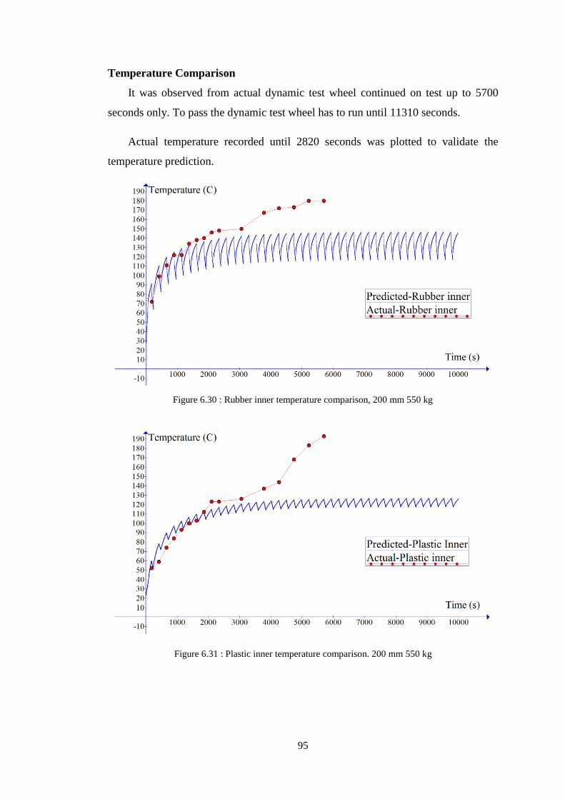
95
Temperature Comparison
It was observed from actual dynamic test wheel continued on test up to 5700
seconds only. To pass the dynamic test wheel has to run until 11310 seconds.
Actual temperature recorded until 2820 seconds was plotted to validate the
temperature prediction.
Figure 6.30 : Rubber inner temperature comparison, 200 mm 550 kg
Figure 6.31 : Plastic inner temperature comparison. 200 mm 550 kg

96
It was observed from actual rubber inner and actual plastic inner graph, wheel
continued temperature development even after predicted steady state level. No
prominent steady state level was observed from those temperatures also. Castor wheel
failure was evaluated to check weather wheel was yielded before entering steady state
level which would lead to observed type performance.
Figure 6.32 : Plastic outer temperature comparison, 200 mm 550 kg
Figure 6.33 : Rubber outer temperature comparison, 200 mm 550 kg

97
Failure Analysis
From initial static load analysis plastic center was stressed up to 26.4 MPa. From
2D axisymmetric static loading simulation required load was calculated to stress the
center to same level. 4515 N was required to be applied on 2D model to stress center
up to 26.4 MPa von Mises stress. Temperature data were loaded to the model and
failure analysis was carried out to evaluate wheel failure at steady state level.
Maximum 26.7 MPa von Mises stress was observed in the center part of the wheel
at steady state level. Same place was identified as highest temperature of 127 oC
recorded at steady state level. Safety factor analysis was done to evaluate yielding of
the wheel at steady state level.
Table 6.9 : 200 mm 550 kg safety factor
From safety factor analysis, it was observed that plastic was yielded when entering
steady state level. Since plastic yields before steady state level in actual test, which
cause the continuous increase of actual test temperatures and failing before required
run time.
MPa MPa
Equivalent load
Stress in nylon centre
Nylon yield stress at
127oC
Safety factor
for nylon centre
550 kg 26.7 25.3 0.94
Figure 6.34 : 200 mm 550 kg stress distribution at steady state

98
7. Discussion
Castor wheels which are tested in dynamic test procedure goes through several
stages which was identified by physical testing and temperature development curves.
Initially rapid temperature development phase was observed followed by steady state
temperature region. After continuing in steady state level, temperature raised again due
to yielding and bounce of the wheel when wheel was close to fail.
Developed temperature prediction model was capable of confidently predicting
rapid temperature development phase and steady state phase of the castor wheels in
dynamic testing. Simulation model was developed to extract data form static FEA
simulations and DMA test data for temperature prediction. Similar models were
proposed for pneumatic tyres in previous researches such as [9], [7] .
In this research FEA dynamic loading energy rate was captured by static loading
FEA simulation. Then correction factor and wheel rotations were applied to convert
captured static energy data to dynamic analysis. Because of this method, developed
model can be used with mid-range FEA software also. Steady state FEA analysis with
mixed Eulerian/Lagrangian reference frame was used to calculate dynamic energy rate
in most literature which is only available with high end expensive FEA software [19]
another method was modeling of full tyre and simulating the actual rotation behavior
under given load and velocity which consumes lots of computer resources and time
[9].
DMA experiment results and calculations obtained in this research was found to
be closely matching with literature data and applications for FEA simulation [9].
Castor wheel failure analysis model was developed to predict failures at steady state
level. From the model safety factor of the wheel at steady state level was extracted.
von Mises failure criterion was used to evaluate this safety factor of the castor wheel.
Failure evaluation by von Mises criterion is common practice and from literate also
von Mises stress was used to evaluate stress inside rubber tyres [7], [9].

99
Validation of failure was done for both passed and failed wheel in actual dynamic
test and was found to be having close relation with finite element model results. Case
study 1 and 2 showed prominent steady state temperature levels matching with actual
physical data. In case study 3 and 4 prominent steady state level was not observed in
actual temperature records. When analyzed by failure simulation it was observed that
these wheels start to yield when wheel comes to steady state level. This observation
suggest in actual wheel will continue in temperature development region and fail,
which was validated by comparing temperature profiles in case study 3 and 4. From
all case studies it was found that when safety factor was below 1 wheel failed in actual
test. Passed wheels in dynamic test showed 1.61, 1.12 and 1.41 safety factors at steady
state level. So it was decided to keep safety factor above 1.1 for good performing
designs.
FEA elements and material models used for rubber and plastic materials were
based on literature data and was validated by closely matching results for temperature
prediction model in this research. Several literatures were found where developed FEA
models were validated by comparing predicted temperature graphs with test data [19],
[9], [8].
FEA model was developed analyzing rubber and plastic materials. Developed
model can be used with other material castor wheels such as polyurethane,
thermoplastic rubber with relevant raw material testing for given materials. But further
validation is required to evaluate the accuracy of the model on those areas.
Developed temperature prediction and failure analysis model can be used in castor
wheel designs to develop optimized designs and to reduce trial and error costs. Also,
it’s recommended to use this model on existing designs to identify potential
weaknesses and possible improvements.
Simulation tests were carried out on core i5-4590 3.3 GHz computer with 8 GB
ram. Model setup time, manual calculations and static 3D simulation consumed 90%
of time while all 2D axisymmetric simulations took only 10% of total simulation time.
By incorporating 2D axisymmetric simulations whenever possible in to the model,
simulation time of a design kept to a minimum.

100
8. Conclusions
Developed finite element model was validated to be used with rubber castor wheels
made from plastic centers which are tested in dynamic test. Safety factor of 1.1 was
selected to be used in design when wheels are loaded at steady state temperature levels.
Model can be customized to do dynamic test with different run-stop cycle, test speed
and different loads by inputting relevant data to the model.
Model was able to predict temperature development and failure of a given castor
wheel design within 8 hrs. With help of the developed model, quick competitive prices
can be offered to the customer requests to secure new requests. New wheel
development cycle which was 1.5 to 3 months long was reduced to 2 weeks with 70%
saving which accounts for Rs.350,000 from trial moulds and testing in general for
single wheel development. Rs. 3.5 million can be saved per year if company gets ten
new development requirements.
Further opportunities for research was identified in castor wheel failure area to
develop a simulation model to predict actual wheel failure start time after wheel
achieves steady state level which involves very complex material behaviors, material
damage models and practical variations in steady state region.
By using the steps followed its possible to develop simulation models for other
rubber tyres such and pneumatic tyres, solid tyres which goes through same type of
standard tests with appropriate model parameters and modifications.

101
Bibliography
[1] "Castors & Wheels | Castors Online | TENTE USA", Tente.com, 2016.
[Online]. Available: https://www.tente.com/us-us/.
[2] Export Development Board (EDB), Sri Lanka, "Sri Lankan rubber product
sector," Colombo, 2016.
[3] J. K. S. Sankalpa, "Export performance of rubber products manufacturing
sector," Journal of the Rubber Research Institute of Sri Lanka, vol. 93, pp. 51-
61, 2013.
[4] The ICWM Performance Standard for Casters and Wheels, ANSI Standard
ICWM:2012.
[5] Castors and wheels. test methods and apparatus, BS EN Standard 12527:1999.
[6] Castors and wheels. Castors and wheels for applications up to 1,1 m/s (4
km/h), BS EN Standard 12532:1999.
[7] N. Korunovi, M. Trajanovi, and M. Stojkovi, “Finite Element Model for
Steady-State Rolling Tire Analysis,” Serbian Soc. Comput. Mech., vol. 1, no. 1,
pp. 63–79, 2007.
[8] T. Ebbott, "Tire temperature and rolling resistance prediction with finite
element," Tire Science and Technology, vol. 27, no. 01, pp. 2-21, 1999.
[9] Y. J. Lin and S. J. Hwang, “Temperature prediction of rolling tires by computer
simulation,” Math. Comput. Simul., vol. 67, no. 3, pp. 235–249, 2004.
[10] K. Ioi, "Study on Shimmy Vibrations of Wheeled Casters," International
Journal of Materials, Mechanics and Manufacturing, vol. 03, no. 02, pp. 92-
96, 2015.
102
[11] T. Frank, "Measurement of the turning, rolling and obstacle resistance of
wheelchair castor wheels," Journal of Biomedical Engineering, vol. 11, no. 6,
pp. 462-466, 1989.
[12] I. Evans, "The rolling resistance of a wheel with a solid rubber tyre," British
Journal of Applied Physics, vol. 5, no. 5.
[13] J. v. Oosten, "Time, tire measurements forces and moments: a new standard for
steady state cornering tyre testing," in EAEC Congress: 'Vehicle systems
technology for the next century', Barcelona, Spain, 1999.
[14] R. Trivini, "Hubless castor wheel construction". USA Patent US7657969 B2,
10 02 2010.
[15] C. L. Steven Lewis, "Caster wheel having integrated braking means". USA
Patent US7712184 B1, 11 05 2010.
[16] M. Shiraishi, "Method for pneumatic tire simulation". USA Patent
US20070137290 A1, 21 06 2007.
[17] Y. Nakajima, "Application of Computational Mechanics to Tire Design—
Yesterday, Today, and Tomorrow," Tire Science and Technology, vol. 34, no.
04, pp. 223-244, 2011.
[18] N. Korunović, "Finite Element Analysis of a Tire Steady Rolling on the Drum,"
Journal of Mechanical Engineering, pp. 888-897, 2011.
[19] R. E. Smith, T. Tang, D. Johnson, E. Ledbury, T. Goddette, and S. D. Felicelli,
“Simulation of Thermal Signature of Tires and Tracks,” in Proceedings of the
2012 NDIA ground vehicle systems engineering and technology, 2012.
[20] U. Suripa, "Finite element stress and strain analysis of a solid tyre," Journal of
Achievements in Materials and Manufacturing Engineering, vol. 31, no. 02, pp.
576-579, 2008.

103
[21] M. s. Bani, "Prediction of heat generation in rubber and rubber to metal
springs," Thermal science, vol. 16, no. 02, pp. 527-539, 2012.
[22] "www.tiniusolsen.com," [Online]. Available: https://www.tiniusolsen.com/list-
of-products/model-5-st. [Accessed 05 10 2016].
[23] Kevin P. Menard, Dynamic mechanical analyse: A practical introduction, New
York: CRC Press LCC, 1999.
[24] Dynamic Mechanical Analysis (DMA) Basics and Beyond,PerkinElmer Inc.,
2000.
[25] D. H. “. Qi, "Finite Element Analysis," 2006. [Online]. Available:
http://www.colorado.edu/MCEN/MCEN4173/chap_01.pdf. [Accessed 2016].
[26] Strand 7 Theoretical manual, 1st ed., Strand 7, Sydney, 2004.
[27] F. Ebrahimi, "http://www.intechopen.com/," 10 2012. [Online]. Available:
http://www.intechopen.com/books/finite-element-analysis-applications-in-
mechanical-engineering/overview-in-the-application-of-fem-in-mining-and-
the-study-of-case-stress-analysis-in-pulleys-of-sta. [Accessed 2016].
[28] C. Aparicio, "MSC Software," 2013. [Online]. Available:
http://simulatemore.mscsoftware.com/advanced-contact-modeling-in-fea-marc-
video/. [Accessed 04 2016].
[29] www.engineersedge.com, "Engineers Edge," 2016. [Online]. Available:
http://www.engineersedge.com/material_science/von_mises.htm. [Accessed 05
2016].
[30] Wolfram Research, Inc, "Wolfram Mathworld," Wolfram Research, Inc, 1999-
2016. [Online]. Available: http://mathworld.wolfram.com/RiemannSum.html.
[Accessed 06 2016].

104
[31] Intec, "Physical Properties of Metals vs. Plastics and tempreature effects,"
2014. [Online]. Available: http://www.intechpower.com/material-
information/effects-of-temperature. [Accessed 07 2016].
[32] T. R. M. R. A. Pavan, "High performance polymer blends," Milan Italy, 2003.

105
Appendix 1 – Sample wheels dynamic test results summary

106
Appendix 2 – Static loading energy calculation case study 1
m N N Nm Nm
Increment Displacement Force Forcex4 Step Energy Sum of Energy 1 0.0000 0.00 0.00
2 0.0001 1.19 4.75 0.0005
3 0.0002 4.08 16.31 0.0017
4 0.0003 8.58 34.31 0.0035
5 0.0004 15.27 61.06 0.0062
6 0.0005 24.22 96.89 0.0099
7 0.0006 35.10 140.40 0.0143
8 0.0007 47.57 190.27 0.0194
9 0.0008 61.61 246.42 0.0251
10 0.0009 76.97 307.87 0.0314
11 0.0010 93.81 375.25 0.0383
12 0.0011 111.94 447.74 0.0457
13 0.0012 131.47 525.89 0.0537
14 0.0013 152.54 610.15 0.0623
15 0.0014 175.10 700.41 0.0715
16 0.0015 199.04 796.15 0.0812
17 0.0016 224.06 896.23 0.0915
18 0.0017 250.59 1002.35 0.1023
19 0.0018 278.34 1113.37 0.1136
20 0.0019 307.61 1230.46 0.1256
21 0.0020 338.24 1352.97 0.1381
22 0.0021 370.21 1480.83 0.1511
23 0.0022 403.35 1613.40 0.1646
24 0.0023 437.93 1751.73 0.1787
25 0.0024 473.74 1894.97 0.1934
26 0.0026 511.11 2044.45 0.2086
27 0.0027 550.26 2201.05 0.2246
28 0.0028 590.80 2363.20 0.2411
29 0.0029 632.54 2530.18 0.2582
30 0.0030 675.68 2702.72 0.2758
31 0.0031 720.04 2880.15 0.2939
32 0.0032 765.89 3063.56 0.3126
33 0.0033 812.98 3251.93 0.3318
34 0.0034 861.44 3445.77 0.3516
35 0.0035 911.83 3647.32 0.3722
36 0.0036 963.51 3854.05 0.3933
37 0.0037 1016.51 4066.06 0.4149

107
38 0.0038 1070.76 4283.06 0.4370
39 0.0039 1126.46 4505.83 0.4598 6.30
40 0.0040 1183.48 4733.90 0.4830
41 0.0041 1241.88 4967.51 0.5069 7.29
42 0.0042 1301.61 5206.44 0.5313
43 0.0043 1362.75 5450.99 0.5562 8.38
44 0.0044 1425.27 5701.07 0.5818
45 0.0045 1489.68 5958.72 0.6080
46 0.0046 1555.68 6222.72 0.6350
47 0.0047 1623.12 6492.47 0.6625
48 0.0048 1691.83 6767.32 0.6905
49 0.0049 1762.00 7048.01 0.7192
50 0.0050 1833.63 7334.53 0.7484
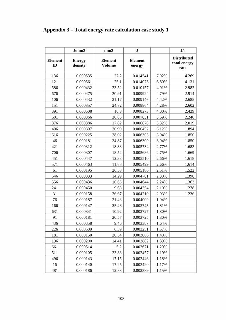
108
Appendix 3 – Total energy rate calculation case study 1
J/mm3 mm3 J J/s
Element
ID Energy
density Element
Volume Element
energy
Distributed
total energy
rate
136 0.000535 27.2 0.014541 7.02% 4.269
121 0.000561 25.1 0.014073 6.80% 4.131
586 0.000432 23.52 0.010157 4.91% 2.982
676 0.000475 20.91 0.009924 4.79% 2.914
106 0.000432 21.17 0.009146 4.42% 2.685
151 0.000357 24.82 0.008864 4.28% 2.602
391 0.000508 16.3 0.008273 4.00% 2.429
601 0.000366 20.86 0.007631 3.69% 2.240
376 0.000386 17.82 0.006878 3.32% 2.019
406 0.000307 20.99 0.006452 3.12% 1.894
616 0.000225 28.02 0.006303 3.04% 1.850
46 0.000181 34.87 0.006300 3.04% 1.850
421 0.000312 18.38 0.005734 2.77% 1.683
706 0.000307 18.52 0.005686 2.75% 1.669
451 0.000447 12.33 0.005510 2.66% 1.618
571 0.000463 11.88 0.005499 2.66% 1.614
61 0.000195 26.53 0.005186 2.51% 1.522
646 0.000333 14.29 0.004761 2.30% 1.398
556 0.000436 10.66 0.004644 2.24% 1.363
241 0.000450 9.68 0.004354 2.10% 1.278
31 0.000158 26.67 0.004210 2.03% 1.236
76 0.000187 21.48 0.004009 1.94%
166 0.000147 25.46 0.003745 1.81%
631 0.000341 10.92 0.003727 1.80%
91 0.000181 20.57 0.003725 1.80%
436 0.000358 9.46 0.003387 1.64%
226 0.000509 6.39 0.003251 1.57%
181 0.000150 20.54 0.003086 1.49%
196 0.000200 14.41 0.002882 1.39%
661 0.000514 5.2 0.002671 1.29%
511 0.000105 23.38 0.002457 1.19%
496 0.000143 17.15 0.002446 1.18%
16 0.000140 17.25 0.002420 1.17%
481 0.000186 12.83 0.002389 1.15%

109
211 0.000286 7.15 0.002046 0.99%
1 0.000110 16.3 0.001790 0.86%
691 0.000392 4.39 0.001722 0.83%
526 0.000078 19.96 0.001564 0.76%
466 0.000221 6.66 0.001472 0.71%
256 0.000160 6.15 0.000985 0.48%
541 0.000069 9.83 0.000680 0.33%
301 0.000033 15.15 0.000503 0.24%
316 0.000031 16.16 0.000501 0.24%
331 0.000026 13.72 0.000362 0.17%
286 0.000033 10.85 0.000361 0.17%
361 0.000033 9.2 0.000308 0.15%
271 0.000032 6.13 0.000196 0.09%
346 0.000022 8.84 0.000191 0.09%

110
Appendix 4 – Material property data
Material thermal properties
Material Mass
Density Specific Heat
capacity Heat
conductivity Forced
Convection-Air
Rubber to floor
conduction
kg/mm3 W/kg/k W/mm/c W/mm2/ c ◦ W/mm2/ c ◦
PP 0.00000091 1800 0.00018 0.0000060
Nylon 0.00000125 1700 0.00026 0.0000060
NR-1 0.0000012 1700 0.000239 0.0000060 0.0001
NR-2 0.0000012 1700 0.000239 0.0000060 0.0001
Nylon
Temperature (oC) Modulus(MPa) Yield (MPa)
23 821.2 68.4
140 614.0 19.9
Polypropylene
Temperature (oC) Modulus(MPa) Yield (MPa)
23 194.5 24.6
120 152.0 9.2

111
Appendix 5 – Static load energy calculation case study 2
m N N Nm Nm
Increment Displacement Force Forcex4 Step
Energy Sum of Energy
1 0.00010 0 0.00
2 0.00020 1.257258 5.03 0.0005
3 0.00030 3.84284 15.37 0.0015
4 0.00040 7.206436 28.83 0.0029
5 0.00050 11.40075 45.60 0.0046
6 0.00060 16.24889 65.00 0.0065
7 0.00070 21.98813 87.95 0.0088
8 0.00080 28.48838 113.95 0.0114
9 0.00090 35.47014 141.88 0.0142
10 0.00100 43.02067 172.08 0.0172
11 0.00110 51.48609 205.94 0.0206
12 0.00120 60.42285 241.69 0.0242
13 0.00130 69.90346 279.61 0.0280
14 0.00140 79.80058 319.20 0.0319
15 0.00150 90.56133 362.25 0.0362
16 0.00160 101.9456 407.78 0.0408
17 0.00170 113.855 455.42 0.0455
18 0.00180 126.2865 505.15 0.0505
19 0.00190 139.0828 556.33 0.0556
20 0.00200 152.2478 608.99 0.0609
21 0.00210 166.0777 664.31 0.0664
22 0.00220 180.4575 721.83 0.0722
23 0.00230 195.2797 781.12 0.0781
24 0.00240 210.6726 842.69 0.0843
25 0.00250 226.3694 905.48 0.0905
26 0.00260 242.4892 969.96 0.0970
27 0.00270 258.9483 1035.79 0.1036
28 0.00280 275.9915 1103.97 0.1104
29 0.00290 293.4132 1173.65 0.1174
30 0.00300 311.2933 1245.17 0.1245 1.41
31 0.00310 329.5096 1318.04 0.1318
32 0.00320 348.092 1392.37 0.1392
33 0.00330 367.0028 1468.01 0.1468
34 0.00340 386.1508 1544.60 0.1545
35 0.00350 405.5723 1622.29 0.1622

112
36 0.00360 425.4024 1701.61 0.1702
37 0.00370 445.7278 1782.91 0.1783
38 0.00380 466.2945 1865.18 0.1865
39 0.00390 487.0827 1948.33 0.1948
40 0.00400 508.1855 2032.74 0.2033
41 0.00410 529.505 2118.02 0.2118
42 0.00420 550.992 2203.97 0.2204
43 0.00430 572.9177 2291.67 0.2292
44 0.00440 595.0815 2380.33 0.2380
45 0.00450 617.4105 2469.64 0.2470
46 0.00460 639.9348 2559.74 0.2560
47 0.00470 662.8398 2651.36 0.2651
48 0.00480 685.9876 2743.95 0.2744
49 0.00490 709.2901 2837.16 0.2837
50 0.00500 732.814 2931.26 0.2931

113
Appendix 6 – Total energy rate calculation case study 2
j/mm3 mm3 j j/s
Element ID Energy density
Element Volume
Element energy
Distributed
total energy rate
316 0.000265870 10.6077 0.002820266 8.11% 1.292
331 0.000252908 9.67325 0.002446438 7.04% 1.121
301 0.000203095 11.7425 0.002384842 6.86% 1.093
1006 0.000192424 12.2099 0.002349472 6.76% 1.076
1021 0.000230018 10.1773 0.002340966 6.73% 1.073
991 0.000149435 13.6587 0.002041084 5.87% 0.935
346 0.000204574 9.3742 0.001917716 5.52% 0.879
1036 0.000209048 8.47719 0.001772136 5.10% 0.812
1111 0.000160948 9.9696 0.001604584 4.62% 0.735
361 0.000137740 9.8194 0.001352526 3.89% 0.620
721 0.000166655 8.02756 0.001337835 3.85% 0.613
271 0.000085904 13.5214 0.001161544 3.34% 0.532
286 0.000087106 12.792 0.001114260 3.21% 0.511
496 0.000111334 9.30384 0.001035835 2.98% 0.475
256 0.000070042 13.6411 0.000955448 2.75% 0.438
1051 0.000143685 6.48561 0.000931886 2.68% 0.427
976 0.000062597 12.9214 0.000808836 2.33% 0.371
736 0.000112505 5.41065 0.000608726 1.75%
376 0.000058295 10.4366 0.000608400 1.75%
1081 0.000100734 5.55336 0.000559409 1.61%
391 0.000046323 9.66751 0.000447824 1.29%
241 0.000034355 12.2522 0.000420926 1.21%
586 0.000075645 5.45711 0.000412806 1.19%
1096 0.000062330 5.46608 0.000340701 0.98%
1066 0.000090956 3.65384 0.000332339 0.96%
751 0.000069900 3.05763 0.000213727 0.61%
406 0.000028449 6.67923 0.000190017 0.55%
871 0.000068980 2.6912 0.000185640 0.53%
766 0.000050072 2.857 0.000143057 0.41%
511 0.000039924 3.28712 0.000131234 0.38%
886 0.000052473 2.47377 0.000129806 0.37%
226 0.000012054 9.44255 0.000113816 0.33%
646 0.000052992 2.08619 0.000110551 0.32%
856 0.000058347 1.66181 0.000096962 0.28%
901 0.000025591 3.33241 0.000085278 0.25%
661 0.000041102 2.07454 0.000085267 0.25%

114
421 0.000018083 4.28921 0.000077561 0.22%
841 0.000044893 1.4802 0.000066451 0.19%
166 0.000010322 6.13154 0.000063293 0.18%
781 0.000032610 1.88477 0.000061462 0.18%
826 0.000031427 1.87331 0.000058873 0.17%
811 0.000036671 1.48722 0.000054538 0.16%
526 0.000022276 2.3696 0.000052785 0.15%
961 0.000005143 8.72056 0.000044851 0.13%
211 0.000007167 5.92793 0.000042485 0.12%
181 0.000005758 7.18575 0.000041379 0.12%
151 0.000007802 5.04791 0.000039383 0.11%
796 0.000021629 1.7508 0.000037869 0.11%
631 0.000022445 1.63264 0.000036644 0.11%
76 0.000033536 1.06177 0.000035607 0.10%
436 0.000012839 2.74106 0.000035192 0.10%
676 0.000011942 2.70406 0.000032293 0.09%
601 0.000014803 2.02524 0.000029979 0.09%
196 0.000005037 5.58552 0.000028134 0.08%
916 0.000004477 6.26928 0.000028069 0.08%
91 0.000022565 1.24036 0.000027989 0.08%
61 0.000026557 1.02183 0.000027136 0.08%
106 0.000011736 2.04604 0.000024012 0.07%
931 0.000003762 5.67673 0.000021357 0.06%
616 0.000015749 1.31141 0.000020653 0.06%
946 0.000004227 4.79977 0.000020287 0.06%
121 0.000005494 3.13512 0.000017223 0.05%
706 0.000003193 4.97009 0.000015870 0.05%
451 0.000009152 1.65951 0.000015188 0.04%
1141 0.000011233 1.32921 0.000014932 0.04%
541 0.000008620 1.70588 0.000014705 0.04%
136 0.000003133 4.24859 0.000013311 0.04%
46 0.000017865 0.711695 0.000012715 0.04%
466 0.000005754 2.19612 0.000012636 0.04%
1 0.000004916 1.54294 0.000007585 0.02%
481 0.000004284 1.76682 0.000007570 0.02%
556 0.000005440 1.23487 0.000006718 0.02%
691 0.000001495 4.08363 0.000006104 0.02%
571 0.000004028 1.36092 0.000005482 0.02%
16 0.000004377 1.21743 0.000005329 0.02%
31 0.000006565 0.722598 0.000004744 0.01%
1126 0.000007526 0.457442 0.000003443 0.01%

115
Appendix 7 - Static load energy calculation case study 3
m N N Nm Nm
Increment Displacement Force Forcex4 Step Energy Sum of Energy
1 0.0000 0.00 0.00
2 0.0001 1.24 4.95 0.0005
3 0.0002 3.61 14.43 0.0015
4 0.0003 6.92 27.69 0.0028
5 0.0004 10.96 43.84 0.0045
6 0.0005 15.91 63.63 0.0065
7 0.0006 21.56 86.24 0.0088
8 0.0007 27.73 110.93 0.0113
9 0.0008 34.80 139.20 0.0142
10 0.0009 42.66 170.65 0.0174
11 0.0010 50.92 203.66 0.0208
12 0.0011 60.01 240.05 0.0245
13 0.0012 69.88 279.53 0.0285
14 0.0013 80.41 321.64 0.0328
15 0.0014 91.25 364.99 0.0372
16 0.0015 102.79 411.15 0.0420
17 0.0016 115.23 460.91 0.0470
18 0.0017 128.24 512.95 0.0523
19 0.0018 141.86 567.43 0.0579
20 0.0019 155.82 623.27 0.0636
21 0.0020 170.52 682.10 0.0696
22 0.0021 185.93 743.71 0.0759
23 0.0022 201.87 807.46 0.0824
24 0.0023 218.26 873.05 0.0891
25 0.0024 235.22 940.88 0.0960
26 0.0025 252.60 1010.40 0.0516 0.9387
27 0.0026 270.47 1081.89 0.1082
28 0.0027 288.98 1155.92 0.1156
29 0.0028 308.11 1232.42 0.1232

116
Appendix 8 - Total energy rate calculation case study 3
mm3 j/mm3 j j/s
Element
ID
Element
Volume
Energy
density
Element
energy
Distributed
total energy
rate
316 7.18371 0.00027528 0.0019776 8.28% 1.083
331 6.6234 0.00026892 0.0017811 7.46% 0.976
631 7.50451 0.00023269 0.0017462 7.31% 0.957
301 7.46889 0.00020512 0.0015320 6.41% 0.839
646 6.7869 0.00021239 0.0014415 6.04% 0.790
616 7.33481 0.00018974 0.0013917 5.83% 0.762
346 5.8648 0.00022742 0.0013338 5.58% 0.731
601 6.47454 0.00015446 0.0010000 4.19% 0.548
661 5.47471 0.00017820 0.0009756 4.08% 0.534
1066 5.32881 0.00016825 0.0008966 3.75% 0.491
361 5.30246 0.00016385 0.0008688 3.64% 0.476
286 7.97832 0.00008470 0.0006757 2.83% 0.370
271 7.92035 0.00008106 0.0006420 2.69% 0.352
676 4.88749 0.00013070 0.0006388 2.67% 0.350
586 6.01317 0.00010380 0.0006242 2.61% 0.342
1186 4.617 0.00013388 0.0006181 2.59% 0.339
256 7.55159 0.00007050 0.0005324 2.23% 0.292
1051 4.49976 0.00011087 0.0004989 2.09% 0.273
871 4.50944 0.00010767 0.0004855 2.03% 0.266
376 4.88574 0.00007644 0.0003735 1.56%
241 7.21567 0.00004904 0.0003539 1.48%
691 4.26953 0.00007678 0.0003278 1.37%
1081 3.01122 0.00009651 0.0002906 1.22%
391 4.56164 0.00006133 0.0002798 1.17%

117
Appendix 9 - Static load energy calculation case study 4
m N N Nm Nm
Increment Displacement Force Forcex4 Step Energy
Sum of
Energy
1 0.0000 0.0 0.00
2 0.0002 2.4 9.73 0.0019
3 0.0004 7.3 29.03 0.0058
4 0.0006 15.0 60.17 0.0120
5 0.0008 24.5 98.15 0.0196
6 0.0010 36.1 144.37 0.0289
7 0.0012 50.2 201.00 0.0402
8 0.0014 65.9 263.52 0.0527
9 0.0016 82.7 330.63 0.0661
10 0.0018 100.8 403.32 0.0807
11 0.0020 119.9 479.73 0.0959
12 0.0022 140.1 560.34 0.1121
13 0.0024 161.8 647.03 0.1294
14 0.0026 184.4 737.49 0.1475
15 0.0028 207.6 830.40 0.1661
16 0.0030 231.6 926.36 0.1853
17 0.0032 257.0 1028.10 0.2056
18 0.0034 283.3 1133.16 0.2266
19 0.0036 310.4 1241.59 0.2483
20 0.0038 338.4 1353.44 0.2707
21 0.0040 367.1 1468.44 0.2937
22 0.0042 397.1 1588.45 0.3177
23 0.0044 428.3 1713.25 0.3426
24 0.0046 460.2 1840.62 0.3681
25 0.0048 492.7 1970.88 0.3942
26 0.0050 525.7 2102.99 0.4206
27 0.0052 560.1 2240.39 0.4481
28 0.0054 595.8 2383.01 0.4766
29 0.0056 632.0 2527.91 0.5056
30 0.0058 669.0 2675.83 0.5352
31 0.0060 706.7 2826.63 0.5653
32 0.0062 744.8 2979.35 0.5959
33 0.0064 784.3 3137.02 0.6274
34 0.0066 824.4 3297.67 0.6595
35 0.0068 866.4 3465.58 0.6931

118
36 0.0070 909.3 3637.31 0.7275
37 0.0072 952.8 3811.24 0.7622
38 0.0074 996.9 3987.54 0.7975
39 0.0076 1042.1 4168.26 0.8337
40 0.0078 1088.2 4352.90 0.8706
41 0.0080 1135.1 4540.34 0.9081
42 0.0082 1183.6 4734.42 0.9469
43 0.0084 1233.1 4932.32 0.9865
44 0.0086 1283.2 5132.90 1.0266
45 0.0088 1334.0 5336.15 1.0672
46 0.0090 1385.5 5542.12 1.1084 19.4
47 0.0092 1438.0 5751.94 1.1504
48 0.0094 1491.3 5965.39 1.1931
49 0.0096 1545.5 6182.13 1.2364
50 0.0098 1600.9 6403.74 1.2807

119
Appendix 10 - Total energy rate calculation case study 4
mm3 j/mm3 j j/s
Element ID Element
Volume
Energy
density
Element
energy
Distributed total
energy rate
354 10.78 0.00063315 0.0068226 8.28% 10.763
351 9.94 0.00061851 0.0061449 7.46% 9.694
631 11.26 0.00053519 0.0060245 7.31% 9.504
620 11.20 0.00047179 0.0052856 6.41% 8.338
646 10.18 0.00048851 0.0049732 6.04% 7.845
433 11.00 0.00043641 0.0048015 5.83% 7.575
349 8.80 0.00052307 0.0046015 5.58% 7.259
604 9.71 0.00035525 0.0034501 4.19% 5.443
664 8.21 0.00040985 0.0033657 4.08% 5.310
1069 7.99 0.00038698 0.0030932 3.75% 4.880
364 7.95 0.00037685 0.0029973 3.64% 4.728
289 11.97 0.00019480 0.0023313 2.83% 3.678
274 11.88 0.00018643 0.0022149 2.69% 3.494
679 7.33 0.00030061 0.0022038 2.67% 3.477
589 9.02 0.00023875 0.0021534 2.61% 3.397
1189 6.93 0.00030792 0.0021325 2.59% 3.364
259 11.33 0.00016215 0.0018368 2.23% 2.898
1054 6.75 0.00025501 0.0017212 2.09% 2.715
874 6.76 0.00024765 0.0016751 2.03% 2.643
379 7.33 0.00017582 0.0012885 1.56%
244 10.82 0.00011280 0.0012209 1.48%
694 6.40 0.00017660 0.0011310 1.37%
1084 4.52 0.00022197 0.0010026 1.22%
394 6.84 0.00014106 0.0009652 1.17%
Copyright © 2022 FDOKUMEN