Fe-Mg interdiffusion at high pressures in mineral phases ...
277
Fe-Mg interdiffusion at high pressures in mineral phases relevant for the Earth’s mantle Inaugural-Dissertation zur Erlangung des Doktorgrades der Mathematisch-Naturwissenschaftlichen Fakult¨ at der Universit¨ at zu K ¨ oln vorgelegt von Christian Holzapfel aus K¨ oln K¨ oln, 2004
-
Upload
khangminh22 -
Category
Documents
-
view
0 -
download
0
Transcript of Fe-Mg interdiffusion at high pressures in mineral phases ...

Fe-Mg interdiffusion at high pressuresin mineral phases
relevant for the Earth’s mantle
Inaugural-Dissertation
zur
Erlangung des Doktorgrades
der Mathematisch-Naturwissenschaftlichen Fakultat
der Universitat zu Koln
vorgelegt von
Christian Holzapfel
aus Koln
Koln, 2004
2
Berichterstatter: Prof. Dr. H. PalmeProf. Dr. D. C. RubieProf. Dr. L. Bohaty
Tag der mundlichen Prufung: 28.5.2004

Contents
Zusammenfassung 7
Abstract 15
1 Introduction 19
1.1 Motivation . . . . . . . . . . . . . . . . . . . . . . . . . . . . . . . . . . . . . .19
1.2 Theory of diffusion . . . . . . . . . . . . . . . . . . . . . . . . . . . . . . .. . 22
1.2.1 Definition of diffusion . . . . . . . . . . . . . . . . . . . . . . . . . .. 22
1.2.2 Macroscopic theory of diffusion . . . . . . . . . . . . . . . . . .. . . . 22
1.2.3 Microscopic theory of diffusion . . . . . . . . . . . . . . . . . .. . . . 23
1.2.4 Oxygen fugacity dependence . . . . . . . . . . . . . . . . . . . . . .. . 26
1.2.5 Temperature dependence of diffusion . . . . . . . . . . . . . .. . . . . 27
1.2.6 Pressure dependence of diffusion . . . . . . . . . . . . . . . . .. . . . 28
1.2.7 Direction dependence of diffusion . . . . . . . . . . . . . . . .. . . . . 29
1.3 Mineralogical model of the Earth’s mantle . . . . . . . . . . . .. . . . . . . . . 30
1.3.1 Phase stabilities and structures . . . . . . . . . . . . . . . . .. . . . . . 30
1.3.2 Summary of existing diffusion data . . . . . . . . . . . . . . . .. . . . 34
1.4 Aims of the present study . . . . . . . . . . . . . . . . . . . . . . . . . . .. . . 38
2 Experimental Techniques 41
2.1 Introduction . . . . . . . . . . . . . . . . . . . . . . . . . . . . . . . . . . . .. 41
2.2 High pressure experiments: Multi anvil technique . . . . .. . . . . . . . . . . . 42
2.3 Diffusion Couples . . . . . . . . . . . . . . . . . . . . . . . . . . . . . . . .. . 43
2.3.1 Diffusion couples: General remarks . . . . . . . . . . . . . . .. . . . . 43
3

4 CONTENTS
2.3.2 Diffusion couples: Olivine . . . . . . . . . . . . . . . . . . . . . .. . . 45
2.3.3 Diffusion couples: Wadsleyite . . . . . . . . . . . . . . . . . . .. . . . 46
2.3.4 Diffusion couples: Ferropericlase . . . . . . . . . . . . . . .. . . . . . 46
2.3.5 Diffusion couples: (Mg,Fe)SiO3 perovskite . . . . . . . . . . . . . . . . 48
2.4 Capsules . . . . . . . . . . . . . . . . . . . . . . . . . . . . . . . . . . . . . . . 50
2.5 Assemblies used for high pressure diffusion experiments . . . . . . . . . . . . . 53
3 Chemical analysis of diffusion profiles 59
3.1 Choice of analysis techniques . . . . . . . . . . . . . . . . . . . . . .. . . . . . 59
3.2 Electron microprobe analysis (EPMA) . . . . . . . . . . . . . . . .. . . . . . . 60
3.3 Transmission electron microscopy . . . . . . . . . . . . . . . . . .. . . . . . . 62
4 Mathematical treatment of diffusion profiles 67
4.1 General remarks . . . . . . . . . . . . . . . . . . . . . . . . . . . . . . . . . .. 67
4.2 Two semi-infinite media, D constant . . . . . . . . . . . . . . . . .. . . . . . . 68
4.3 Semi-infinite media, D concentration-dependent . . . . .. . . . . . . . . . . . . 71
4.3.1 Boltzmann-Matano analysis . . . . . . . . . . . . . . . . . . . . . .. . 71
4.3.2 Numerical simulations: Finite difference method . . .. . . . . . . . . . 73
5 Results 81
5.1 Introduction . . . . . . . . . . . . . . . . . . . . . . . . . . . . . . . . . . . .. 81
5.2 Olivine . . . . . . . . . . . . . . . . . . . . . . . . . . . . . . . . . . . . . . . 84
5.2.1 Conditions of experiments . . . . . . . . . . . . . . . . . . . . . . .. . 84
5.2.2 Characterization of diffusion couples after the experiments . . . . . . . . 85
5.2.3 Profiles and diffusion coefficients . . . . . . . . . . . . . . . .. . . . . 88
5.2.4 Pressure dependence at constant temperature (1673 K). . . . . . . . . . 93
5.2.5 Temperature dependence at constant pressure (12 GPa). . . . . . . . . . 98
5.2.6 Model of diffusion in olivine . . . . . . . . . . . . . . . . . . . . .. . . 104
5.2.7 Comparison with previous results . . . . . . . . . . . . . . . . .. . . . 105
5.3 Wadsleyite . . . . . . . . . . . . . . . . . . . . . . . . . . . . . . . . . . . . . .109
5.3.1 Conditions of experiments . . . . . . . . . . . . . . . . . . . . . . .. . 109

CONTENTS 5
5.3.2 Backscatter images and sample characterization . . . .. . . . . . . . . . 110
5.3.3 Profiles . . . . . . . . . . . . . . . . . . . . . . . . . . . . . . . . . . . 113
5.3.4 Temperature dependence at 15 GPa . . . . . . . . . . . . . . . . . .. . 115
5.3.5 Summary: Fe-Mg interdiffusion in wadsleyite . . . . . . .. . . . . . . . 119
5.4 Ferropericlase . . . . . . . . . . . . . . . . . . . . . . . . . . . . . . . . . .. . 121
5.4.1 Conditions of experiments . . . . . . . . . . . . . . . . . . . . . . .. . 121
5.4.2 Sample characterization . . . . . . . . . . . . . . . . . . . . . . . .. . 122
5.4.3 Profiles and diffusion coefficients . . . . . . . . . . . . . . . .. . . . . 123
5.4.4 Pressure dependence at constant temperature . . . . . . .. . . . . . . . 128
5.4.5 Temperature dependence at constant pressure . . . . . . .. . . . . . . . 129
5.4.6 Oxygen fugacity . . . . . . . . . . . . . . . . . . . . . . . . . . . . . . 132
5.4.7 Summary: Ferropericlase . . . . . . . . . . . . . . . . . . . . . . . .. . 132
5.5 (FexMg1−x)SiO3 Perovskite . . . . . . . . . . . . . . . . . . . . . . . . . . . . . 135
5.5.1 Introduction, conditions of experiments . . . . . . . . . .. . . . . . . . 135
5.5.2 SEM and EPMA investigations of perovskite diffusion experiments . . . 135
5.5.3 TEM characterization of the samples . . . . . . . . . . . . . . .. . . . 142
5.5.4 Profiles and diffusion coefficients . . . . . . . . . . . . . . . .. . . . . 144
5.5.5 Temperature dependence of Fe-Mg interdiffusion at 24GPa . . . . . . . 150
5.6 Overview . . . . . . . . . . . . . . . . . . . . . . . . . . . . . . . . . . . . . . 154
5.7 Experimental complications . . . . . . . . . . . . . . . . . . . . . . .. . . . . 155
5.7.1 High pressure versus low pressure experiments . . . . . .. . . . . . . . 155
5.7.2 Temperature gradients . . . . . . . . . . . . . . . . . . . . . . . . . .. 155
5.7.3 Heating effects . . . . . . . . . . . . . . . . . . . . . . . . . . . . . . . 157
6 Discussion 159
6.1 Introduction . . . . . . . . . . . . . . . . . . . . . . . . . . . . . . . . . . . .. 159
6.2 Extrapolations towards lower mantle conditions . . . . . .. . . . . . . . . . . . 160
6.2.1 Ferropericlase . . . . . . . . . . . . . . . . . . . . . . . . . . . . . . . .160
6.2.2 Silicate perovskite . . . . . . . . . . . . . . . . . . . . . . . . . . . .. 162
6.3 Fe-Mg interdiffusion along a present day geotherm . . . . .. . . . . . . . . . . 163

6 CONTENTS
6.4 Time scales of Fe-Mg partitioning experiments . . . . . . . .. . . . . . . . . . 167
6.5 Applications to geological problems . . . . . . . . . . . . . . . .. . . . . . . . 169
6.5.1 Kinetics of the olivine-wadsleyite phase boundary . .. . . . . . . . . . 169
6.5.2 Two-phase aggregates . . . . . . . . . . . . . . . . . . . . . . . . . . .172
6.5.3 Reequilibration in the lower mantle . . . . . . . . . . . . . . .. . . . . 178
6.5.4 Interaction at the core-mantle boundary . . . . . . . . . . .. . . . . . . 182
6.5.5 Interaction during core formation . . . . . . . . . . . . . . . .. . . . . 185
7 Conclusions 191
A Multianvil Technique 193
B TEMQuant: Quantifying EDX-TEM analysis 199
B.1 Principles of the program . . . . . . . . . . . . . . . . . . . . . . . . . .. . . . 199
B.2 Source code of TEMQuant . . . . . . . . . . . . . . . . . . . . . . . . . . . .. 200
B.2.1 Header file of class TEMQuant . . . . . . . . . . . . . . . . . . . . . .. 200
B.2.2 Definition of class methods for class TEMQuant . . . . . . .. . . . . . 201
B.2.3 Main function . . . . . . . . . . . . . . . . . . . . . . . . . . . . . . . . 213
C Finite difference simulation 215
C.1 Introduction . . . . . . . . . . . . . . . . . . . . . . . . . . . . . . . . . . . .. 215
C.2 Source code . . . . . . . . . . . . . . . . . . . . . . . . . . . . . . . . . . . . . 216
D Example profile analyses 227
E Example EDX-spectra of silicate perovskite 249
Bibliography 252
Index 272

Zusammenfassung
Zur Quantifizierung der Kinetik vieler Prozesse, wie z.B. Reaquilibrierung subduzierter Platten
oder Phasenumwandlungen mehrkomponentiger Systeme, ist die Kenntnis von Diffusionskoef-
fizienten als Funktion von Druck (P), Temperatur (T), und Sauerstofffugazitat (f O2) unabding-
bar. In dieser Arbeit werden Experimente zur Bestimmung vonFe-Mg Interdiffusionskoeffizien-
ten DFe−Mg bei Drucken zwischen 6 und 23 GPa und Temperaturen von 1653 bis 2273 K bei
reduzierenden und oxidierenden Bedingungen beschrieben.Dabei wurden Diffusionspaare von
Mineralen, die einen wesentlichen Anteil am Mineralbestand des Erdmantels haben, untersucht:
Olivin, Wadsleyit, Ferroperiklas und Silikat-Perowskit.Die wesentlichen Zielsetzungen der Ar-
beit lauteten:
• Bestimmung von Fe-Mg Interdiffusionskoeffizienten in Olivin im gesamten Druck-
Stabilitatsbereich. Außerdem sollten Diffusionskoeffizienten der Spurenelemente Ni und
Mn bestimmt werden
• Bestimmung der Aktivierungsenergie von Wadsleyit
• Bestimmung von Fe-Mg Interdiffusionskoeffizienten fur Ferroperiklas, die zweithaufigste
Phase des unteren Erdmantels
• Bestimmung von Fe-Mg Interdiffusionskoeffizienten fur (Fe,Mg)SiO3 Perowskit, der
haufigsten Phase des unteren Erdmantels
Diffusion unter hohen Drucken kann im wesentlichen durch die folgende Gleichung
beschrieben werden:
D = D0 ( f O2)1n exp(A X) exp
(
−Ea−P∆Va
R T
)
, (1)
7
8 Zusammenfassung
wobei D den Diffusionskoeffizienten,D0 den praexponentiellen Faktor,f O2 die Sauer-
stofffugazitat,n den Sauerstofffugazitatskoeffizienten,A den Koeffizienten der Zusammenset-
zungsabhangigkeit,Ea die Aktivierungsenergie,∆Va das Aktivierungsvolumen,P den Druck,T
die Temperatur und R die Gaskonstante bezeichnen.
Die Hochdruckexperimente dieser Arbeit wurden mit der Vielstempel-Technologie (multi-
anvil apparatus) am Bayerischen Geoinstitut in Bayreuth durchgefuhrt. Die Probe befindet sich
in einem Oktaeder aus MgO, der innerhalb eines Satzes von 8 WC-Wurfeln mit abgeschragten
Ecken komprimiert wird. Die charakteristischen Grossen,die das Volumen der Proben und den
maximal erreichbaren Druck charakterisieren sind die KantenlangeKo des Oktaeders undKa der
Abschragungen des Wurfels. Daher werden die verwendenten Oktaeder mit dem TupelKo/Ka
bezeichnet. In dieser Arbeit wurden Oktaeder mit den Geometrien 18/11, 14/8 und 10/4 ver-
wendet. Zum Heizen wurde eine Widerstandsheizung aus LaCrO3 verwendet. Die Temperatur
wurde wahrend der Experimente mit einem W97Re3-W75Re25 Thermoelement gemessen.
Fur die Herstellung der Diffusionspaare von Olivin wurdenfur jeden Versuch ein Diffusions-
paar aus denselben, in c-Richtung orientierten Einkristallen verwendet. Der Mg-reiche Kristall
war ein synthetischer Forsterit und der Fe-reiche Kristallein San Carlos Olivin mitXFe2SiO4 =
0.06 (XFe2SiO4 bezeichnet den Molenbruch der Fayalit-Komponente im Olivin). Auch die Dif-
fusionspaare von Ferroperiklas wurden aus Einkristallen hergestellt. Eisenhaltige (Mg,Fe)O
Einkristalle mit einem nominalen Gehalt vonXFeO = 0.07 undXFeO = 0.35 sind vor den Dif-
fusionsversuchen von S. Mackwell mit dem in Holzapfel et al.(2003) beschriebenen Verfahren
synthetisiert worden. Fur Wadsleyit und Silikatperowskit wurden polykristalline Proben vor
den eigentlichen Diffusionsversuchen synthetisiert, da es keine naturlichen Proben gibt und eine
Einkristallsynthese nicht erfolgreich war.
Da der Diffusionskoeffizient nach Gleichung 1 von der Sauerstofffugazitat abhangt, wurden
im wesentlichen Kapselmaterialien verwendet, die eine Charakterisierung der Sauerstofffugazitat
wahrend des Experiments zulassen. Zum einen wurden daher Ni-Kapseln mit einer Zugabe von
NiO benutzt, die die Sauerstofffugazitat nahe des Ni-NiO Gleichgewichts puffern. Desweiteren
wurden bei den Perowskit-Versuchen auch MgO-Einkristallkapseln mit einer zusatzlichen Fe-
Folie eingesetzt. Die Sauerstofffugazitat ist dann durchdie Losung von FeO in MgO bestimmt.

Zusammenfassung 9
Nur fur einige Versuche mit Olivin wurden auch Au-Kapseln wie bei Chakraborty et al. (1999)
verwendet. Die Redox-Bedingungen, die in diesen Kapseln vorherrschen, wurden durch Ver-
gleich mit den Resultaten von Experimenten in Ni-NiO-Kapseln charakterisiert.
Nach den Hochdruckversuchen wurden die Diffusionspaare zur Messung mit mikroana-
lytischen Verfahren im Querschliff freigelegt. Fur Profillangen großer als 8µm wurde die
Elektronenstrahl-Mikrosonde eingesetzt (EPMA). Bei einigen Proben, insbesondere bei Silikat-
perowskit, waren die Profile kurzer als die Auflosung die mit EPMA erreicht werden kann. Da-
her wurden diese Proben fur transmissionselektronenmikroskopische Untersuchungen (TEM)
gedunnt. Im Rastermodus (STEM) wurden dann Profilanalysenmit einem EDX-Detektor
durchgefuhrt (EDX-STEM).
Aus den gemessenen Profilen wurden die Diffusionskoeffizienten mit Hilfe unterschiedlicher
mathematischer Verfahren bestimmt. Fur Olivin und Silikat-Perowskit wurden im wesentlichen
symmetrische Profile beobachtet, die mit einer analytischen Losung der Diffusionsgleichung
fur konzentrationsunabhangige Diffusion angepasst wurden. Konzentrationsabhangige Diffu-
sion fuhrte im Fall von Ferroperiklas und Wadsleyit zu asymmetrischen Profilen, fur die keine
analytische Losung existiert. In diesem Fall wurden die Profile numerisch mit Hilfe der finiten
Differenzmethode simuliert. Wadsleyit und Ferroperiklasmit XFeO> 0.07 zeigen eine exponen-
tielle Konzentrationsabhangigkeit des Diffusionskoeffizienten. Nur im Fall von Ferroperiklas
mit XFeO < 0.07 mußte nach Mackwell et al. (2004) ein zusatzlicher Term in die Konzentra-
tionsabangigkeit des Diffusionskoeffizienten eingefuhrt werden.
Fur Olivin wird im wesentlichen eine lineare Abnahme des Fe-Mg Interdiffusionskoeffizien-
ten bis 12 GPa beobachtet. Die Fe-Mg Interdiffusionskoeffizienten, die in Ni-NiO Kapseln
beobachtet wurden, sind im Rahmen des Fehlers identisch mitden Ergebnissen von Versuchen
in Au-Kapseln. Daher kann geschlussfolgert werden, daß dieSauerstofffugazitat, die charakter-
istisch fur die Goldkapseln ist, nahe bei der des Ni-NiO Puffers liegt. Eine Meßreihe mit Olivin
bei 12 GPa und zwischen 1623 K und 1823 K ist ebenfalls kompatibel mit der Aktivierungsen-
ergie bei 1 bar und einer Sauerstofffugazitat nahe des Ni-NiO Puffers. Das Aktivierungsvolumen
entlang des Ni-NiO Puffers ist 5.6±0.5 cm3 mol−1. Wenn man die Sauerstofffugazitat des Ni-
NiO Puffers als Funktion von Druck und Temperatur mit der Annahme eines konstanten Reak-
10 Zusammenfassung
tionsvolumens der Oxidationsreaktion von Ni berucksichtigt, erhalt man ein Aktivierungvolumen
von 7.3±1.0 cm3 mol−1 bei konstanter Sauerstofffugazitat.
Fe-Mg Interdiffusion in Wadsleyit ist wesentlich schneller als in Olivin, wie auch schon
bei Chakraborty et al. (1999) und Farber et al. (2000) beobachtet worden ist. In dieser Arbeit
wird ein Sprung der Diffusivitat um nahezu 4 Großenordnungen bei Bedingungen der 410 km
Diskontinuitat beobachtet. Die Aktivierungsenergie bei15 GPa betragt 260±30 kJ mol−1 (ohne
Korrektur fur den Effekt der Sauerstofffugazitat des Ni-NiO Puffers).
Fur Ferroperiklas wurden Experimente zwischen 8 und 23 GPabei 1663 K bis 2073 K
durchgefuhrt. Die Ergebnisse sind inUbereinstimmung mit Experimenten bei 1 bar (Mackwell
et al., 2004). Fur Sauerstofffugazitaten entlang des Ni-NiO-Puffers wurde ein Aktivierungsvol-
umen von 3.3± 0.1 cm3 mol−1 und eine Aktivierungsenergie von 255 kJ mol−1 bestimmt.
Das Aktivierungsvolumen bei konstanter Sauerstofffugazitat betragt 5± 1 cm3 mol−1. Die
Zusammensetzungsabhangigkeit kann im Bereich zwischen 7und 35 mol%, ubereinstimmend
mit Mackwell et al. (2004) mit einem exponentiellen Ansatz beschrieben werden:DFe−Mg ∝
exp(
(132±13) kJ mol−1 XFeO/(RT))
.
Silikat-Perowskit zeigt deutlich niedrigere Diffusionskoeffizienten als die anderen betrach-
teten Systeme. Der praexponentielle Faktor bei Sauerstofffugazitaten entsprechend des Ni-NiO
Puffers ist(5.1±2.0)×10−8 m2 sec−1 und die Aktivierungsenergie 404±144 kJ mol−1. Damit
sind die Diffusionskoeffizienten des Silikatperowskits, der die Hauptphase des unteren Erdman-
tels bildet, bei denselben P, T undf O2-Bedingungen um etwa einen Faktor 2×10⁴ kleiner als die
von Ferroperiklas. Weil Ferroperiklas nur ungefahr 20 vol% des unteren Erdmantels einnimmt,
werden kinetische Prozesse, die durch Fe-Mg Interdiffusion bestimmt werden, dominiert durch
DFe−Mg von Perowskit. Simulationen in Verbindung mit theoretischen Modellen zeigen, daß der
effektive Diffusionskoeffizient des unteren Erdmantels∼ 2.4×Dpvskbetragt.
Die in dieser Arbeit bestimmten Diffusionskoeffizienten k¨onnen in einer vielseitigen Weise
zur Quantifizierung kinetischer Prozesse, die in der Erde ablaufen oder abgelaufen sind ver-
wendet werden. Dabei verlaufen Prozesse, die von der Geschwindigkeit des Fe-Mg Aus-
tausches abhangen, am schnellsten im Stabilitatsfeld von Wadsleyit und Ringwoodit (410 - 670
km Tiefe). Olivin im oberen Mantel besitzt deutlich kleinere Diffusionskoeffizienten. Bei 12

Zusammenfassung 11
GPa fuhrt der Druckeffekt zu einer Verringerung der Diffusivitat von Olivin um etwa zwei
Grossenordnungen im Vergleich zuDFe−Mg bei 1 bar und derselben Temperatur. Daher sollte
fur kinetische Modellierungen der Druckeffekt nicht vernachlassigt werden. Modellierungen der
Kinetik der Phasenumwandlung von Olivin nach Wadsleyit oder umgekehrt wahrend Konvektion
durch die 410 km Diskontinuitat zeigen, dass die Diffusionskoeffizienten groß genug sind, um bei
einer Konvektionsgeschwindigkeit von 5 cm/Jahr fur eine Gleichgewichtseinstellung zu sorgen.
Allerdings kann es bei deutlich niedrigeren Temperaturen zu einem metastabilenUberschreiten
der Gleichgewichtsphasengrenzen und damit zu einer Verbreiterung der Diskontinuitat kommen.
Fur den unteren Erdmantel (P> 23 GPa) kann die Druckabhangigkeit der Fe-Mg Interdif-
fusion fur Ferroperiklas mit Hilfe von ab initio Berechnungen fur Migrations-Enthalpien und
-Entropien von Ita and Cohen (1997) abgeschatzt werden. Allerdings wird bei diesen Ab-
schatzungen vorausgesetzt, dass bzgl. der Druckabhangigkeit die Berechnung fur Mg Selbst-
diffusion zumindest annahernd auch fur Fe-Mg Interdiffusion gelten. Es zeigt sich, dass nach
Ita and Cohen (1997) die Druckabhangigkeit des praexponentiellen Vorfaktors vernachlassigbar
ist. Damit kann die Druckabangigkeit von∆Va mit einem einfachen quadratischen Ansatz
beschrieben werden. Die Extrapolation des Fe-Mg Interdiffusionskoeffizienten fuhrt entlang
einer Manteladiabate zu einer Abnahme der Diffusivitat imoberen Teil des unteren Erdman-
tels aufgrund des Druckeffektes. Im unteren Bereich des unteren Erdmantels geht das Ak-
tivierungsvolumen nahezu gegen null und der Temperaturanstieg fuhrt zu einer Zunahme des
Diffusionskoeffizienten. Insgesamt variiert der so berechnete Interdiffusionkoeffizient von Fer-
roperiklas um weniger als einen Faktor von 10. Daher ist ein mittlerer Diffusionskoeffizient
von 4× 10⁻¹⁴ m2 sec−1 bei XFeO= 0.1 und einer Sauerstofffugazitat, die dem Ni-NiO Puffer
entspricht, eine gute Naherung furDFe−Mg im unteren Erdmantel.
Fur Silikatperowskit konnte aufgrund des begrenzenten Druckbereiches, der mit Hilfe der
Vielstempel-Technik untersucht werden konnte, kein Aktivierungsvolumen bestimmt werden.
Daher wurden in dieser Arbeit zwei Grenzfalle betrachtet:Der Druckeffekt wird vernachlassigt
(∆Va = 0) oder es wird ein Wert von∆Va = 2.1 cm3 mol−1 (Wright and Price, 1993) angenom-
men. Im ersten Fall steigt entlang einer Manteladiabate dieDiffusivitat von∼ 10−18 m2 sec−1
bei 24 GPa auf 5×10⁻¹⁵ m2 sec−1 bei 136 GPa. Im zweiten Fall (∆Va = 2.1 cm3 sec−1) wird auf-

12 Zusammenfassung
grund des gegensatzlichen Temperatur- und Druckeffektesein im wesentlichen konstanter Fe-Mg
Interdiffusionskoeffizient (∼ 10−18 m2 sec−1) beobachtet. Diese Werte gelten bei einer Sauer-
stofffugazitat entsprechend des Ni-NiO Puffers. Fur reduzierende Verhaltnisse, die ungefahr der
heutigen Fe-Verteilung zwischen Kern und Mantel der Erde entsprechen, istDFe−Mg um etwa
einen Faktor 14 kleiner.
Da die Kinetik im unteren Mantel im wesentlichen vonDFe−Mg von Silikatperowskit
abhangt, zeigen die in dieser Arbeit bestimmten Diffusionskoeffizienten, daß keine effek-
tive Reaquilibrierung im unteren Erdmantel durch reine Volumendiffusion stattfinden kann.
Reaquilibrierungsdistanzen sind selbst auf einer Zeitskala der gesamten Erdgeschichte nicht viel
großer als 1 m. Da diese Werte mit Fe-Mg Interdiffusionskoeffizienten abgeschatzt wurden, sind
fur Elemente wie Ni oder Co ahnliche Werte zu erwarten. Fur Elemente mit großerem Ionenra-
dius und/oder hoherer Wertigkeit wie Ca, Rb, Sr, Nd, Hf oderW werden noch kurzere Distanzen
erwartet, weil im allgemeinen der Diffusionskoeffizient f¨ur diese Elemente kleiner alsDFe−Mg
ist. Damit konnten Teile der ozeanischen Kruste oder kontinentale Sedimente, die durch Subduk-
tion in den unteren Mantel gelangen, sehr lange als eigenst¨andige chemische Signatur bestehen,
sofern kein andererAquilibrierungsmechanismus als Volumendiffusion wirksam wird.
Die maximal mogliche Entfernung eines chemischen Austausches an der Kern-Mantelgrenze
betragt∼ 800 m. Dieser Wert ist nur dann gultig, wenn fur Silikatperowskit ein moglicher Druck-
effekt vernachlassigt wird (∆Va = 0) und die Temperatur in der thermischen Grenzschicht an der
Kern-Mantel-Grenze bei etwa 5000 K liegt. Ansonsten werdenwesentlich niedrigere Werte fur
die Austauschlange abgeschatzt. Damit zeigen die Resultate dieser Arbeit, daß im Laufe der
Erdgeschichte kein effektiver Austausch zwischen Erdkernund Erdmantel alleine durch Volu-
mendiffusion stattgefunden haben kann.
Als letzter Punkt wird in dieser Arbeit eine mogliche Reaquilibrierung nach einer Gleich-
gewichtseinstellung von siderophilen Elementen unter hohen Drucken in einem Magmenozean
betrachtet. Das flussige Metall muß den festen unteren Erdmantel passieren, um den Kern der
Erde zu bilden. Die Diffusionskoeffizienten, die in dieser Arbeit bestimmt wurden, zeigen,
daß im Fall einer Separierung in Form großer Diapire keine signifikante Veranderung der El-
ementhaufigkeiten stattfindet, wohingegen im Falle der Perkolation sich eine neue Verteilung
Zusammenfassung 13
einstellt und die ursprungliche Signatur zerstort wird.In der Zukunft mussen weitere Studien
durchgefuhrt werden, um die Frage der Benetzungswinkel imunteren Erdmantel eindeutig zu
klaren und damit eine bessere geochemische Antwort auf dieVerteilung der siderophilen Ele-
mente zwischen Erdkern und Erdmantel der Erde finden zu konnen.

14 Zusammenfassung
Abstract
In this study Fe-Mg interdiffusion coefficients were determined at pressures between 6 and 26
GPa and temperatures between 1653 and 2273 K for various constituent minerals of the Earth’s
mantle employing a multianvil apparatus. Minerals investigated include olivine, wadsleyite, fer-
ropericlase and (Mg,Fe)SiO3 silicate perovskite. The main aims of this study were:
• To extend the existing diffusion data set for olivine to pressures in excess of 8 GPa.
• To constrain the activation energy for diffusion in wadsleyite over a larger temperature
interval than that of the previous study of Chakraborty et al. (1999).
• To determine Fe-Mg interdiffusion coefficients for ferropericlase, the second most abun-
dant phase in the Earth, over a wide pressure range up to 23 GPa.
• To determine Fe-Mg interdiffusion coefficients for silicate perovskite, the most abundant
mineral in the Earth.
For ferropericlase and olivine, single crystal diffusion couples were used whereas for wads-
leyite and silicate perovskite only presynthesized polycrystalline diffusion couples could be em-
ployed. In the case of olivine, diffusion along the c crystallographic direction was investigated.
As capsule material, Au and Ni-NiO capsules were chosen for olivine and Ni-NiO capsules for
wadsleyite, ferropericlase and silicate perovskite. In addition, in the case of perovskite, single
crystal MgO capsules in contact with metallic Fe were employed. Therefore, because the oxy-
gen fugacity was not fixed at a constant value but varied with the solid state buffers Ni-NiO and
Fe-(Mg,Fe)O with pressure and temperature, activation energies and activation volumes include
this variation in f O2. To retrieve activation energies and volumes at constantf O2, a correction
15

16 Abstract
was performed but is subject to large uncertainties becauseof a lack of a calibration of the buffer
systems at the conditions of the experiments.
Diffusion profiles were measured after the diffusion experiments either by electron micro-
probe analysis (EPMA) or for profiles< 8 µm long by energy dispersive X-ray spectrometry on
a transmission electron microscope equipped with a scanning unit (EDX-STEM). In the case of
olivine and silicate perovskite, diffusion coefficients were found to be essentially constant within
the compositional range investigated resulting in symmetrical diffusion profiles. In this case,
the profiles were fitted with an analytical solution to the diffusion equation. On the other hand,
wadsleyite and ferropericlase exhibited strongly asymmetric profiles implying a strong composi-
tion dependence of Fe-Mg interdiffusion. For elucidating the compositional dependence, profiles
were simulated using the finite difference method.
The activation volume of olivine along the Ni-NiO buffer wasconstrained to be 5.6±0.5 cm3 mol−1. A f O2 correction leads to an activation volume of 7.4± 1.0 cm3 mol−1 at
constantf O2. The temperature effect observed at 12 GPa in Au capsules is consistent with the
1 bar activation energy employing a pressure andf O2 correction. This observation leads to
the conclusion that results obtained from Au capsule experiments (Chakraborty et al., 1999) are
consistent with anf O2 at the Ni-NiO buffer.
Therefore, results obtained for wadsleyite at 15 GPa and 1673-1773 K in Ni-NiO cap-
sules were combined with the previous results by Chakraborty et al. (1999) resulting in an
activation energy of 260± 30 kJ mol−1 along the Ni-NiO buffer at 15 GPa. The composi-
tional dependence of diffusion is stronger than for olivineand can be described by a factor of
exp{(11.8±1.5)XFe2SiO4}, whereXFe2SiO4 is the mole fraction of Fe2SiO4 in the solid solution.
Ferropericlase experiments were performed over a pressurerange between 8 and 23 GPa
leading to an activation volume of 3.3±0.1 cm3 mol−1 along the Ni-NiO buffer. This value cor-
responds to an activation volume of 5±1 cm3 mol−1 at constantf O2. The activation energy was
determined to be 255±16 kJ mol−1 along the Ni-NiO buffer and the compositional dependence
of exp{
(132±13) kJ mol−1 XFeO/(RT)}
, whereXFeO is the mole fraction of FeO, was found to
be consistent with a model at 1 bar of Mackwell et al. (2004).

Abstract 17
Fe-Mg interdiffusion in (Mg,Fe)SiO3 perovskite is orders of magnitude slower than in the
other investigated phases. At oxygen fugacity conditions of the Ni-NiO buffer, the preexponential
factor is(5.1±2.0)×10−8 m2 sec−1 and the activation energy is 404±144 kJ mol−1. Compared
to ferropericlase withXFeO= 0.05−0.1 the difference in the Fe-Mg interdiffusion coefficient is
on the order of a factor of 2×10⁴, with the smaller diffusion coefficient in perovskite. Because
perovskite is believed to be the dominant phase in the lower mantle (∼ 80 vol%), the effective
diffusion coefficientDe f f of the lower mantle should be mainly determined by the diffusion
coefficient of perovskite. An effective diffusion coefficient of De f f = 2.4×Dpvskwas estimated
assuming that ferropericlase occurs as isolated grains.
The very low rates of diffusion in silicate perovskite and hence in the lower mantle implies
that reequilibration kinetics in the lower mantle are very slow. Detailed calculations show that
even on the time scale of the age of the Earth (4.5×10⁹ years) the reequilibration distance is
only∼ 1 m. Therefore, chemical heterogeneities in the lower mantle, resulting for example from
subduction, cannot effectively be erased by lattice diffusion alone. Only in the thermal boundary
layer at the core-mantle boundary larger interaction distances (∼ 10-800 m), depending on the
model used, might exist. During core formation, extensive reequilibration of percolating liquid
metal in the lower mantle occurs on timescales of∼ 100000 years whereas large diapirs would
never reach a new equilibrium state with surrounding oxidesand silicates.

18 Abstract
Chapter 1
Introduction
1.1 Motivation
For a given chemical system at constant pressure and temperature, the Gibbs free energy is
the thermodynamic potential that determines what phases are stable (e.g. Denbigh, 1981). In
nature and technology, systems are often displaced in pressure and temperature space and the
system has to reach a new equilibrium state. Such processes in the mantle of the Earth would
be rising plumes, descending subduction slabs, or reequilibration of minerals with percolating
fluids and melts. The time scale, over which reequilibrationoccurs, is determined by kinetics.
Many such processes are rate limited by diffusion. Therefore understanding diffusion is essential
in constraining time scales of processes and life times of heterogeneities and thermodynamic
disequilibria.
Most diffusion studies on naturally occurring minerals have been performed at 1 bar, ex-
ploring the temperature and composition dependence (Section 1.3.2). In contrast, the pressure
dependence is not well constrained due to experimental difficulties such as keeping pressure and
temperature conditions of diffusion experiments constantfor a long time or having large enough
sample space to accomodate diffusion couples. Hence, the effect of pressure on diffusion is often
neglected. For geological processes occurring in the Earth’s crust, this assumption might be jus-
tified judging from previously reported activation volumesof diffusion, but ignoring the pressure
dependence may lead to substantial errors for processes occurring at greater depth in the Earth’s
mantle or core. For example in Misener (1974) an activation volume for Fe-Mg interdiffusion of
5.5 cm3 mol−1 was determined experimentally, leading to a decrease of diffusivity of 2 orders of
19

20 CHAPTER 1. INTRODUCTION
magnitude over a pressure interval of 12 GPa at 1673 K. Hence,the equilibration timeteq would
be 2 orders of magnitude longer in the upper mantle just abovethe transition zone for the same
diffusional length scalexdi f as compared to processes occurring at the Earth’s surface because
xdi f ∝√
Dteq, where D is the diffusion coefficient.
The effect of pressure on diffusion might influence, for example, calculations of entrap-
ment of melt inclusions and subsequent polybaric reequilibration where normally pressure-
independent expressions for diffusivity are applied (e.g.Cottrell et al., 2002; Gaetani and Watson,
2002). The simulation of Cottrell et al. (2002) shows that the results are very sensitive to small
variations in the diffusion coefficient for small values of the reduced timeτ = t κs R−2 wheret is
time,κs is the diffusion coefficient in the host phase andR is the radius of the inclusion. Another
example from the (Mg,Fe)2SiO4 system are studies of the kinetics of the phase boundary of the
olivine ⇀↽ wadsleyite transition. The growth of wadsleyite from olivine should be rate limited
by interdiffusion in olivine (Rubie, 1993). In the study of Solomatov and Stevenson (1994) an
Fe-Mg interdiffusion coefficient of 10−10 m2 sec−1 was used whereas, as shown above, extrap-
olation of diffusion data employing the activation volume determined at lower pressures would
predict significantly smaller D values and therefore longertime scales.
Only few diffusion studies exist for high pressure phases, such as silicate perovskite. The
reason for this lack of data is the difficulty of maintaining high pressure and temperature con-
ditions to stabilize the high pressure phases for such a longtime that diffusion profiles can be
measured. Although the diamond anvil cell can reach pressures up to several 100 GPa, equivalent
to conditions of the Earth’s core, the sample volume is not big enough to accomodate diffusion
couples. On the contrary, the multianvil apparatus is capable of fulfilling these requirements up
to pressures of more than 25 GPa and temperatures well above 2000 K. In the last few years the
setup of a new 5000 t multianvil press at the Bayerisches Geoinstitut lead to the possibility of
performing multianvil experiments at stable pressure and temperature conditions on time scales
up to several days with large volume samples (up to 3 mm3 at 22 GPa, Frost et al., 2003). The
experiments reported in this study were performed at pressures between 6 and 26 GPa at tem-
peratures between 1623 K and 2273 K for time durations in the range of 5 minutes up to 3 days.
In combination with microanalytical techniques (Chapter 3), such as the electron microprobe or

1.1. MOTIVATION 21
for smaller length scales the analytical transmission electron microscope (Meißner et al., 1998),
interdiffusion coefficients on the order of 10−20 m2 sec−1 can now be determined with diffusion
couple experiments at pressures as high as 26 GPa with reasonable accuracy.
Only two studies of Fe-Mg interdiffusion in wadsleyite exist in the literature at present
(Chakraborty et al., 1999; Farber et al., 2000). In the studyof Chakraborty et al. (1999) two
experiments are reported, that span a temperature range of only 100 K. The experiments of Far-
ber et al. (2000) were all performed at one temperature. Therefore one aim of this study is to
better constrain the activation energy of Fe-Mg interdiffusion in wadsleyite by performing ex-
periments at higher temperatures than Chakraborty et al. (1999).
Numerous applications of diffusion coefficients exist, such that only a few can be highlighted
in this paragraph. For example, the knowledge of interdiffusion coefficients of the phases form-
ing the lower mantle will help in understanding such fundamental questions as the grain size in
this part of the Earth. In a simulation of the grain size in thelower mantle by Solomatov et al.
(2002), diffusion coefficients for Si self diffusion were taken from Yamazaki et al. (2000). But
up to now it is not established what the slowest diffusing species in silicate perovskite is. For
silicates with SiO4 tetrahedra, Si diffusion is much slower than Fe-Mg interdiffusion (e.g. Brady,
1995). But the structure of silicate perovskite is quite different, containing SiO6 octahedra, (Sec-
tion 1.3.1) and therefore this assumption needs to be tested(for results from a theoretical study
of relative diffusivities in perovskite see section 1.3.2). Fe-Mg partitioning experiments between
magnesiowustite and magnesium silicate perovskite already show that Fe-Mg exchange is a very
slow process in perovskite at least at reducing conditions (Frost and Langenhorst, 2002). The
data on diffusion will be used in section 6.5.5 to constrain kinetically some recently-proposed
core forming scenarios. In these models a magma ocean existsat an early stage of Earth’s his-
tory with a depth of approximately 1000 km. The current distribution of siderophile elements
between the core and the mantle would be established by metal-silicate equilibration at the base
of the magma ocean. Subsequently, after the equilibration event, the liquid metal has to descend
through the solids forming the lower mantle either by large diapirs or by grain boundary wetting.
The extent of reequilibration and hence obliteration of thesiderophile element signature is con-
troled by diffusion in the solids and therefore the knowledge of diffusion coefficients becomes

22 CHAPTER 1. INTRODUCTION
essential in understanding this process.
Results of previous diffusion studies of olivine, wadsleyite, ferropericlase and silicate per-
ovskite are summarized in Section 1.3.2. The most importantaspects of the theory of diffusion,
as needed as a background for this study, are given in the nextsection.
1.2 Theory of diffusion
1.2.1 Definition of diffusion
“Diffusion and mass flow or drift result from individual jumps of atoms and/or point defects
in the solid” (Philibert, 1991). In the case of a crystallinesolid, periodic jumps occur between
distinct lattice sites (Shewmon, 1989). Random walk theorytherefore provides the link between
macroscopic diffusion coefficients, as defined below and experimentally determined in this study,
and microscopic motion of individual atoms in the structure.
1.2.2 Macroscopic theory of diffusion
In a macroscopic linear theory, without considering the atomistic details of the diffusion process,
the diffusion coefficient is defined by Fick’s first law (Fick,1855):
Ji = −Di∇ni (1.1)
whereJi is the flux of component i, in terms of the number of atoms crossing a unit area perpen-
dicular to the flux-direction in unit time,ni is the number of atomsi per unit volume andDi is
the diffusion coefficient for atoms i. Hence, the diffusion coefficient relates the vectorJi to the
vector∇ni, the gradient of the concentration, and is therefore a second rank tensor (Nye, 1985).
When measuring diffusion coefficients in non-cubic materials, the direction dependence has to
be taken into account (see section 1.2.7).
Equation 1.1 is valid at a local point in space and time. Due tothe fact that local fluxes are
difficult to dermine directly, only in very special circumstances, in the case of a local steady state,
can Equation 1.1 be used to determine the diffusion coefficient (e.g. permeation experiments as
described in Philibert, 1991). In the non-steady state, where the concentration distribution is a
function of time, which is the normal situation in a diffusion couple experiment as used in this

1.2. THEORY OF DIFFUSION 23
study (Chapter 2.3), Fick’s second law is used for measuringthe diffusion coefficientDi :
∂ni
∂t= ∇ · (Di∇ni) (1.2)
Equation 1.2 can be derived from Equation 1.1 by consideringthe conservation of atoms i during
the diffusion process (see Allnatt and Lidiard, 1993, for details). Ficks second law is a parabolic
partial differential equation of the second order, mathematically equivalent to Fouriers law of heat
conduction, and solutions for many initial and boundary conditions are listed in Crank (1979) and
Carslaw and Jaeger (1946). For other forces apart from a concentration gradient, Equation 1.1
has to be extended. For any forceF produced by a potential gradientF = −∇V it can be shown
that Equation 1.2 has to be written as (Shewmon, 1989):
∂ni
∂t= Di∇
[
∇ni +n∇VkT
]
(1.3)
if the diffusion coefficientDi is position and concentration-independent. For limitations of the
linear theory (Equation 1.1) see Allnatt and Lidiard (1993).
1.2.3 Microscopic theory of diffusion
Diffusion takes place by the hopping of atoms between lattice sites. For random jumps with
equal probability of jump directions, following Einstein (1905), the diffusion coefficientD in
one direction is related to the mean-square displacement〈X2〉 in a time intervalt by:
D =〈X2〉2t
(1.4)
A number of possible different diffusion mechanisms exist,for example direct exchange, va-
cancy, interstitial, or intersticialcy. Divalent cation diffusion in silicates and oxides is assumed to
occur mostly by a vacancy mechanism. Vacancies are either intrinsically or extrinsically created.
The abundance of intrinsic lattice vacancies varies with temperature and their presence is ther-
modynamically favored because the free energy of the systemis lowered due to mixing effects,
whereas extrinsic vacancies are created by aliovalent substitution or by oxidation of transition
metal ions like Fe (Ganguly, 2002). In an Arrhenius plot a kink is observed with a steeper slope
at high temperature for the intrinsic regime and a shallowerslope for the extrinsic regime at lower
temperature (e.g. in the NaCl system see: Mapother et al., 1950). Buening and Buseck (1973)
24 CHAPTER 1. INTRODUCTION
also observed such a kink in the olivine system, but this observation was later disproved by
Chakraborty (1997, see section 1.3.2). In addition to the classical intrinsic and extrinsic regime,
Chakraborty (1997) proposed an additional regime for Fe-bearing silicates due to the fact that
unlike in a pure extrinsic case the concentration of point defects changes with temperature be-
cause, based on the redox reaction of Fe, the Fe2+/Fe3+ ratio changes with temperature as well.
As a consequence the activation energy comprises a sum of a formation and a migration enery
(like in the intrinsic case). This diffusion regime is termed “transition metal-extrinsic” (TaMED)
by Chakraborty (1997). TaMED posesses both extrinsic (defect concentration is controlled by
a chemical potential at a fixed P,T, and major element composition) and intrinsic (change of
concentratiton of vacancies with P and T) character.
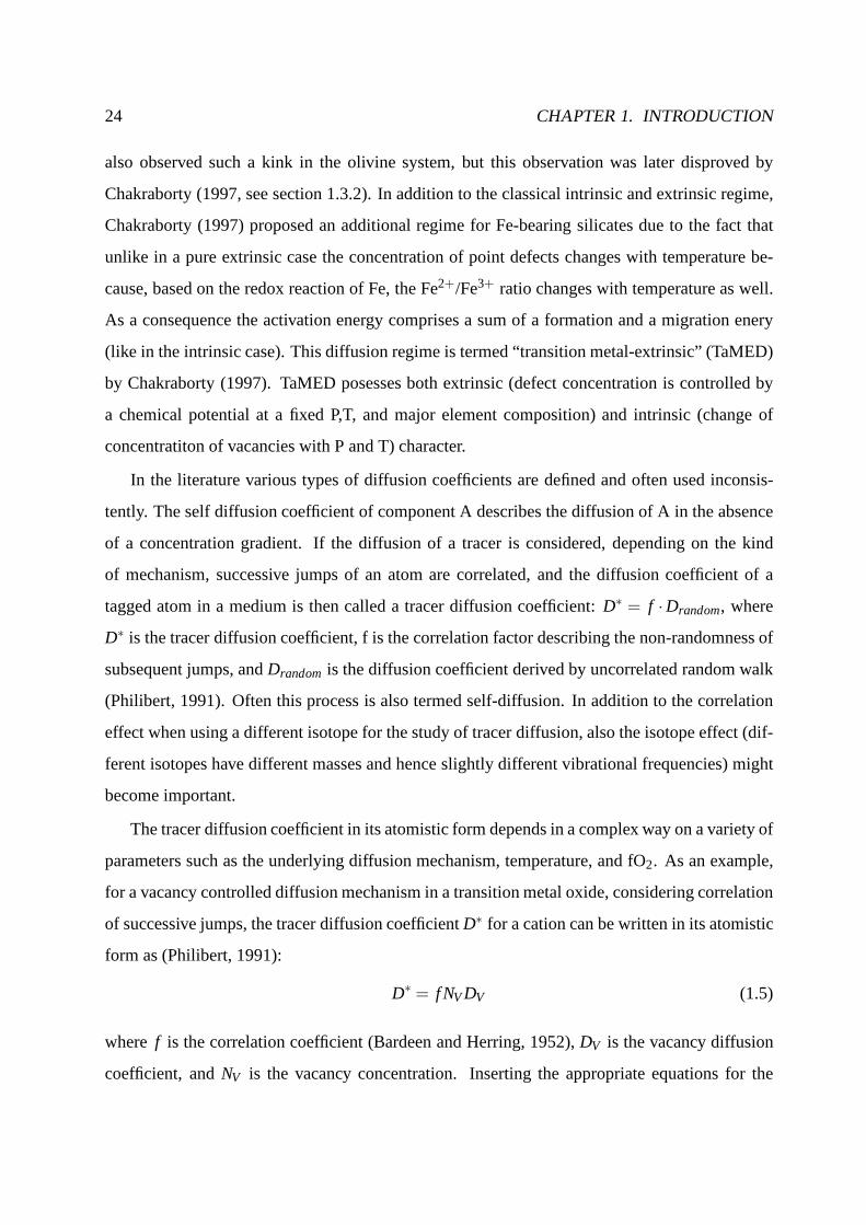
In the literature various types of diffusion coefficients are defined and often used inconsis-
tently. The self diffusion coefficient of component A describes the diffusion of A in the absence
of a concentration gradient. If the diffusion of a tracer is considered, depending on the kind
of mechanism, successive jumps of an atom are correlated, and the diffusion coefficient of a
tagged atom in a medium is then called a tracer diffusion coefficient: D∗ = f ·Drandom, where
D∗ is the tracer diffusion coefficient, f is the correlation factor describing the non-randomness of
subsequent jumps, andDrandom is the diffusion coefficient derived by uncorrelated randomwalk
(Philibert, 1991). Often this process is also termed self-diffusion. In addition to the correlation
effect when using a different isotope for the study of tracerdiffusion, also the isotope effect (dif-
ferent isotopes have different masses and hence slightly different vibrational frequencies) might
become important.
The tracer diffusion coefficient in its atomistic form depends in a complex way on a variety of
parameters such as the underlying diffusion mechanism, temperature, and fO2. As an example,
for a vacancy controlled diffusion mechanism in a transition metal oxide, considering correlation
of successive jumps, the tracer diffusion coefficientD∗ for a cation can be written in its atomistic
form as (Philibert, 1991):
D∗ = f NVDV (1.5)
where f is the correlation coefficient (Bardeen and Herring, 1952),DV is the vacancy diffusion
coefficient, andNV is the vacancy concentration. Inserting the appropriate equations for the

1.2. THEORY OF DIFFUSION 25
vacancy diffusivity and the vacancy abundance (including the fO2 dependence) in Eq. 1.5, the
complete expression for the tracer diffusion coefficient isderived (Philibert, 1991)
D∗ = βa2ν f AV ( fO2)mexp
(
SmV +Sf
V
k
)
exp
(
−HmV +H f
V
kT
)
(1.6)
whereβ is a geometrical factor,a is the lattice constant,ν is a vibration frequency,A is a constant,
m is a constant depending on the charge state of the vacancy,SmV is the vacancy migration entropy,
SfV is the effective vacancy formation entropy (Philibert, 1991), Hm
V is the vacancy migration
enthalpy,H fV is the effective vacancy formation enthalpy,k is Boltzmann’s constant, and T is
temperature (for the pressure dependence see section 1.2.6).
In computer simulations self-diffusion coefficients are calculated employing equations corre-
sponding to Eq. 1.6 using a variety of computer simulation techniques (e.g. Ita and Cohen, 1997;
Vocadlo et al., 1995; Wright and Price, 1989). Although a lot of assumptions have to be made in
order to keep computation times reasonable, comparisons with experimentally determined diffu-
sion coefficients are often relatively encouraging. Therefore, they may be used for extrapolation
of experimentally determined values towards P and T conditions that are not reachable by exper-
iment. This approach is used in Chapter 6 to extrapolate diffusion data to conditions of the lower
mantle.
Most systems are thermodynamically nonideal and in addition to a concentration gradient
other driving forces such as chemical potential gradients (or more precisely the nonideal part of
the chemical potential gradient), stress gradients or temperature gradients exist (as already indi-
cated in Section 1.2.2). The role of stress gradients and temperature gradients in the experiments
of this study are investigated in section 5.7.
Fluxes of different species are usually coupled due to constraints of electroneutrality and
conservation of lattice sites in a crystal. In this study minerals forming Fe-Mg solid solutions are
investigated. Because the flux of Fe-atoms in one direction is coupled with a flux of Mg-atoms in
the other direction (in the microscopic picture also with a flux of vacancies), in a single diffusion
couple experiment, employing two endmember crystals with adifferent Fe-Mg concentration,
only one independent Fe-Mg interdiffusion coefficient can be determined for each profile (Fe
or Mg). In that context the term chemical diffusion is used. Chemical diffusion describes the
exchange of chemical components (Brady, 1975a) and not structure elements in the sense of

26 CHAPTER 1. INTRODUCTION
Schmalzried (1995). Different equations exist for relating chemical diffusion coefficients deter-
mined in interdiffusion studies with microscopically defined self diffusion coefficients depending
on the system under investigation (for metals: Darken (1948), for ionic compounds: Barrer et al.
(1963); Brady (1975a); Manning (1968)). In all of these equations, for a dilute component in a
diffusion couple, the ideal part of the chemical diffusion coefficient equals the tracer diffusion
coefficient of the dilute component (Chakraborty, 1995). Ina nonideal solid solution the situ-
ation becomes more complex because an additional thermodynamic factor has to be included
(Chakraborty, 1995). In Section 5.2 not only Fe-Mg interdiffusion in olivine has been measured
but also the diffusion of the dilute components Ni and Mn weredetermined.
1.2.4 Oxygen fugacity dependence
For most mineral systems in the Earth, it is assumed that cation diffusion occurs via vacancies.
In the case of Fe-bearing solid-solutions the concentration of vacancies is a function of the oxy-
gen fugacity. For example in ferropericlase, (Mg,Fe)O, onemay write according to Chen and
Peterson (1980) and Poirier (2000):
12
(O2)g+2FexMe ⇀↽ Ox
O +V′′M +2Fe•M (1.7)
using the Kroger-Vink notation, where a structure element(Schmalzried, 1995) is described as
Sql with S denotes the atom or point defect,q the electric charge with respect to the perfect lattice
(x = neutral, ’ = negative,• = positive), andl the sublattice on which S resides. With the Fe3+-ion
an electron hole is associated and therefore the equilibrium constantK1.7 of Equation 1.7 can be
written as:
K1.7 =[V
′′M][h•]2
( f O2)12
. (1.8)
The electroneutrality condition is:
2[
V′′M
]
= [h•] . (1.9)
Combining Equations 1.8 and 1.9 and usingD ∝ [V′′M] (compare with Eq. 1.5) leads to the ideal
f O2 dependence:
D ∝ [V′′M] ∝ ( f O2)
16 . (1.10)

1.2. THEORY OF DIFFUSION 27
An equivalent analysis for majority defects in other minerals can be made. A detailed study
for olivine can be found in Nakamura and Schmalzried (1983, 1984). The treatment should be
similar for the high pressure polymorphs of olivine. Silicate perovskite has a much higher Fe3+
content even at low oxygen fugacities. For this phase the situation is more complicated because
Fe3+ can also be incorporated into the Si-site as a coupled substitution or charge balanced by O
vacancies (Lauterbach et al., 2000; Frost and Langenhorst,2002). No rigorous quantitative treat-
ment of the point defect chemistry of Fe-bearing perovskitewith respect to transport properties
so far exists in the literature.
1.2.5 Temperature dependence of diffusion
The diffusion coefficientD depends strongly on temperature because diffusion is a thermally
activated process. Often it is found experimentally thatD follows an Arrhenius relationship:
D = D0 exp
[
− Ea
RT
]
(1.11)
whereD0 is the preexponential factor,Ea is the activation energy, R is the universal molar gas
constant, andT is temperature. Equation 1.11 implies that in a plot of logD versus the inverse
temperature, a linear relationship is observed where the slope gives the activation energy (Fig.
1.1).
The dependence on temperature may be understood in the framework of the theory of the
activated complex. Local fluctuations in energy, responsible for a successful jump of an atom to
another crystal site, occur with a frequency dominated by a Boltzmann exponential factor (All-
natt and Lidiard, 1993). As shown in section 1.2.3 the concentration and mobility of vacancies
depends exponentially on temperature. Hence a diffusion process with a vacancy mechanism
should also be exponentially dependent on temperature (Eq.1.5, 1.6).
Nevertheless one should be aware that the Arrhenius law is not universal, and might break
down in cases where there is a change in diffusion mechanism (extrinsic to intrinsic diffusion
transition, see Section 1.2.3), impurities or microstructural irregularities.
28 CHAPTER 1. INTRODUCTION
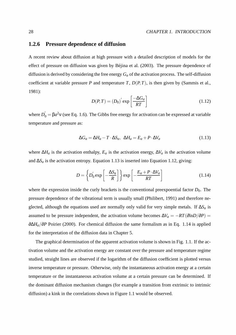
1.2.6 Pressure dependence of diffusion
A recent review about diffusion at high pressure with a detailed description of models for the
effect of pressure on diffusion was given by Bejina et al. (2003). The pressure dependence of
diffusion is derived by considering the free energyGa of the activation process. The self-diffusion
coefficient at variable pressureP and temperatureT, D(P,T), is then given by (Sammis et al.,
1981):
D(P,T) = (D0)′exp
[−∆Ga
RT
]
(1.12)
whereD′0 = βa2ν (see Eq. 1.6). The Gibbs free energy for activation can be expressed at variable
temperature and pressure as:
∆Ga = ∆Ha−T ·∆Sa, ∆Ha = Ea +P ·∆Va (1.13)
where∆Ha is the activation enthalpy,Ea is the activation energy,∆Va is the activation volume
and∆Sa is the activation entropy. Equation 1.13 is inserted into Equation 1.12, giving:
D =
{
D′0exp
[
−∆Sa
R
]}
exp
[
−Ea +P ·∆Va
RT
]
(1.14)
where the expression inside the curly brackets is the conventional preexpoential factorD0. The
pressure dependence of the vibrational term is usually small (Philibert, 1991) and therefore ne-
glected, although the equations used are normally only valid for very simple metals. If∆Sa is
assumed to be pressure independent, the activation volume becomes∆Va = −RT(∂lnD/∂P) =
∂∆Ha/∂P Poirier (2000). For chemical diffusion the same formalism as in Eq. 1.14 is applied
for the interpretation of the diffusion data in Chapter 5.
The graphical determination of the apparent activation volume is shown in Fig. 1.1. If the ac-
tivation volume and the activation energy are constant overthe pressure and temperature regime
studied, straight lines are observed if the logarithm of thediffusion coefficient is plotted versus
inverse temperature or pressure. Otherwise, only the instantaneous activation energy at a certain
temperature or the instantaneous activation volume at a certain pressure can be determined. If
the dominant diffusion mechanism changes (for example a transition from extrinsic to intrinsic
diffusion) a kink in the correlations shown in Figure 1.1 would be observed.

1.2. THEORY OF DIFFUSION 29
6
-
6
-
log10D log10D
1T P
@@
@@
@@
@@
@@
@@
@@@
@@
@@
@@
@@
@@
@@
@@@
m= −Ea+∆Va·(P−Pre f)
2.3026R m= − ∆Va2.3026RT
A B"!#
"!#
Figure 1.1: Graphical interpretation of the activation energy and the activation volume. A:The activation energyEa is calculated from a slope of logD versus the inverse temperatureT.At a pressureP = Pre f = 1 bar the slope directly gives the activation energy whereasat highpressure the slope gives the combined pressure and temperature effect. B: The activationvolumeVa is calculated from the slope of logD versus the pressure.
1.2.7 Direction dependence of diffusion
In Eq. 1.1, Fick’s first law, the diffusion coefficient relates the vector concentration gradient to
the vector flux. Therefore the diffusion coefficient is a second rank tensor. Only for amorphous
or cubic materials the diffusion coefficient is direction-independent. Equation 1.1 can be written
as:
Ji = Di jCj (1.15)
whereJi equals the flux in the i-direction,Cj is the concentration derivative in the j-direction,
the Di j are the corresponding components of the diffusion tensor, and the Einstein summation
convention is assumed (when a letter suffix occurs twice in the same term, summation with re-
spect to that suffix from 1 to 3 is to be automatically understood, Nye, 1985). TheDi j form a
symmetric second rank tensor (Ganguly, 2002) and the independent components for each crystal
system can be found in Nye (1985) or Haussuhl (1983). As discussed in the next section, olivine,
wadsleyite and silicate perovskite are orthorhombic, whereas ferropericlase is cubic. Therefore,
the diffusion coefficient as a second rank tensor does not depend on direction in ferropericlase.

30 CHAPTER 1. INTRODUCTION
For the orthorhombic system three independent components exist, which areD11, D22, andD33
for the normal convention of the crystal-physical coordination system (Nye, 1985).
1.3 Mineralogical model of the Earth’s mantle
1.3.1 Phase stabilities and structures
In Figure 1.2 a section through the Earth’s mantle is shown, outlining the stability ranges of the
most important mineral phases. The upper mantle is dominated by olivine which transforms
at 410 km to its high pressure polymorph wadsleyite. Wadsleyite is stable down to a depth
of approximately 520 km where it transforms to ringwoodite.The olivine phase diagram was
determined by Akaogi et al. (1984), Akaogi et al. (1989), Katsura and Ito (1989), Morishima et al.
(1994), and Suzuki et al. (2000). At 670 km ringwoodite decomposes into silicate perovskite and
ferropericlase (Ito and Takahashi, 1989). The precise depth of this decomposition and the nature
of the 670-km discontinuity is currently debated due to recent in situ multianvil and diamond
anvil studies (Chudinovskikh and Boehler, 2001; Irifune etal., 1998; Katsura et al., 2003; Shim
et al., 2001a). With increasing depth silicate perovskite becomes more Al-rich consuming the
majoritic garnet (Wood, 2000). Pyroxenes are only stable atdepths less than 480 km where they
react to form majorite (Akaogi and Akimoto, 1977). At 580 km Ca-perovskite becomes stable
taking the Ca-component from majoritic garnet (Liu, 1975).A more extensive review about
phase stabilities and mantle discontinuities can be found in Poirier (2000).
As outlined in section 1.1 and is evident from the last paragraph, diffusion coefficients are
needed for the minerals shown in Fig. 1.2 for constraining kinetic processes occurring in the
Earth. This study focuses mainly on Fe-Mg interdiffusion asa function of pressure and tem-
perature in olivine, wadsleyite, silicate perovskite and ferropericlase. In addition, Ni and Mn
diffusion in olivine was also investigated.
Olivine crystallizes in the orthorhombic space group Pbnm.Thus diffusion in olivine is
anisotropic (see section 1.2.7). The oxyen atoms form a distorted hexagonal array parallel to
(100) planes. For the divalent cations two different octahedral sites M1 and M2 exist, where in
(Fe,Mg)2SiO4 solid solutions the larger Fe2+ ion is incorporated preferentially into the smaller
M1 site (Deer et al., 1992). The M1 octahedra form edge-sharing chains along the crystallo-

1.3. MINERALOGICAL MODEL OF THE EARTH’S MANTLE 31
upper mantle/crust
transitionzone
lowermantle
0
20
40
60
80
100
100200300400500600700800
Abu
ndan
ce o
f Min
eral
s, v
olum
e %
Depth, km
olivine
wadsleyite
ringwoodite
majoritic garnet
PyroxeneCa-Perovskite
silicateperovskite
ferro-periclase
A
B
Figure 1.2: Section through the Earth’s mantle. In (A) the abundance of minerals in thedepth-interval 100 - 800 km (redrawn from Jackson and Rigden(1998) with original datafrom Irifune (1993, 1994)), and in (B) a schematical sectionthrough the whole mantle isshown.
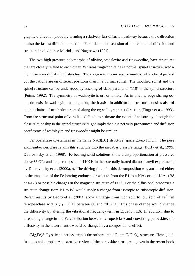
32 CHAPTER 1. INTRODUCTION
graphic c-direction probably forming a relatively fast diffusion pathway because the c-direction
is also the fastest diffusion direction. For a detailed discussion of the relation of diffusion and
structure in olivine see Morioka and Nagasawa (1991).
The two high pressure polymorphs of olivine, wadsleyite andringwoodite, have structures
that are closely related to each other. Whereas ringwooditehas a normal spinel structure, wads-
leyite has a modified spinel structure. The oxygen atoms are approximately cubic closed packed
but the cations are on different positions than in a normal spinel. The modified spinel and the
spinel structure can be understood by stacking of slabs parallel to (110) in the spinel structure
(Putnis, 1992). The symmetry of wadsleyite is orthorhombic. As in olivine, edge sharing oc-
tahedra exist in wadsleyite running along the b-axis. In addition the structure consists also of
double chains of octahedra oriented along the crystallographic a direction (Finger et al., 1993).
From the structural point of view it is difficult to estimate the extent of anisotropy although the
close relationship to the spinel structure might imply thatit is not very pronounced and diffusion
coefficients of wadsleyite and ringwoodite might be similar.
Ferropericlase crystallizes in the halite NaCl(B1) structure, space group Fm3m. The pure
endmember periclase retains this structure into the megabar pressure range (Duffy et al., 1995;
Dubrovinsky et al., 1998). Fe-bearing solid solutions showa disproportionation at pressures
above 85 GPa and temperatures up to 1100 K in the externally heated diamond anvil experiments
by Dubrovinsky et al. (2000a,b). The driving force for this decomposition was attributed either
to the transition of the Fe-bearing endmember wustite fromthe B1 to a NiAs or anti-NiAs (B8
or a-B8) or possible changes in the magnetic structure of Fe2+. For the diffusional properties a
structure change from B1 to B8 would imply a change from isotropic to anisotropic diffusion.
Recent results by Badro et al. (2003) show a change from high spin to low spin of Fe2+ in
ferropericlase withXFeO = 0.17 between 60 and 70 GPa. This phase change would change
the diffusivity by altering the vibrational frequency termin Equation 1.6. In addition, due to
a resulting change in the Fe-distribution between ferropericlase and coexisting perovskite, the
diffusivity in the lower mantle would be changed by a compositional effect.
(Mg,Fe)SiO3 silicate perovskite has the orthorhombic Pbnm GdFeO3-structure. Hence, dif-
fusion is anisotropic. An extensive review of the perovskite structure is given in the recent book

1.3. MINERALOGICAL MODEL OF THE EARTH’S MANTLE 33
by Mitchell (2002). The ideal structure consists of corner linked SiO6 octahedra forming 12-
coordinated cation sites in between the octahedra. The deviation from cubic symmetry occurs by
the tilting of the SiO6 octahedra and displacement of Si from the center of an octahedron. With
respect to diffusion this change in structure is minor when compared to the anisotropic arrange-
ment of edge-charing polyhedra chains e.g. in olivine (see above). Even in olivine the anisotropy
is only approximately a factor of 6 between the slowest direction (b) and the fastest direction
(c) at∼ 1373 K. Therefore the extent of anisotropy in silicate perovskite is expected to be very
small.
In the literature is an ongoing debate about whether there are structural phase transitions for
silicate perovskite at conditions of∼ 25 GPa and elevated temperatures (conditions of the multi-
anvil press used in this study). Wang et al. (1992) concludedin their electron microscopy study
of (Mg,Fe)SiO3 perovskite that, based on twin morphology, analog studies,and theoretically pre-
dicted twin laws, silicate perovskite might be cubic above 1873 K and 26 GPa. However, such a
phase change is not detected in situ by X-ray diffraction in adiamond anvil cell. The most recent
study by Shim et al. (2001b) only shows the possibility of a phase change from the orthorhombic
space group Pbnm, stable at low pressures and temperatures,to either P21/m, Pmmn, or P42/nmc
above 83 GPa and 1973 K.

34 CHAPTER 1. INTRODUCTION
1.3.2 Summary of existing diffusion data
General remarks
The section about existing diffusion data should summarizediffusion data relevant for this study.
This includes mainly Fe-Mg interdiffusion or cation diffusion studies for olivine, wadsleyite,
ferropericlase and silicate perovskite. Numerous studiesfor Si or O diffusion in olivine exist but
are not explicitely cited here because these components were not further investgated in this study.
General reviews for diffusion data covering a large varietyof minerals and different species can
be found in Brady (1995) and especially for other high pressure phases in Bejina et al. (2003).
On the contrary, Mg, Si and O self-diffusion studies in ferropericlase and silicate perovskite are
described to some extent because they are the only existing high pressure data available for these
phases. Especially interesting is the relative differenceof Si and O self-diffusion compared to
Fe-Mg interdiffusion in silicate perovskite.
Olivine
Several studies for diffusion of octahedral cations have been performed at 1 bar and elevated
temperatures and varying oxygen fugacities (Clark and Long, 1971; Buening and Buseck, 1973;
Misener, 1974; Hermeling and Schmalzried, 1984; Nakamura and Schmalzried, 1984; Jurewicz
and Watson, 1988; Morioka and Nagasawa, 1991; Chakraborty,1997; Ito et al., 1999; Petry,
1999a; Petry et al., 2003). Discrepancies that exist between the different datasets are thoroughly
further discussed in Chakraborty (1997). High pressure Fe-Mg interdiffusion experiments have
been performed at pressures up to 3.5 GPa by Misener (1974) and Farber et al. (2000). They
derived activation volumes for Fe-Mg interdiffusion in olivine of 5.5 and 5.4 cm3 mol−1 respec-
tively. Between 3 and 9 GPa, Fe-Mg interdiffusion experiments were performed at very low
temperatures, between 873 and 1173 K, by Jaoul et al. (1995).The experiments employed San
Carlos olivine covered with a thin layer of fayalite and the diffusion profiles were analyzed by
Rutherford backscattering. Errors for the diffusion coefficients reported in Jaoul et al. (1995) are
up to two orders of magnitude. The activation volume deducedwas essentially zero within the er-
ror of the eperiments. Jaoul et al. (1995) attributed the difference in activation volume compared
to the study of Misener (1974) to a change from extrinsic diffusion at low temperatures (Jaoul
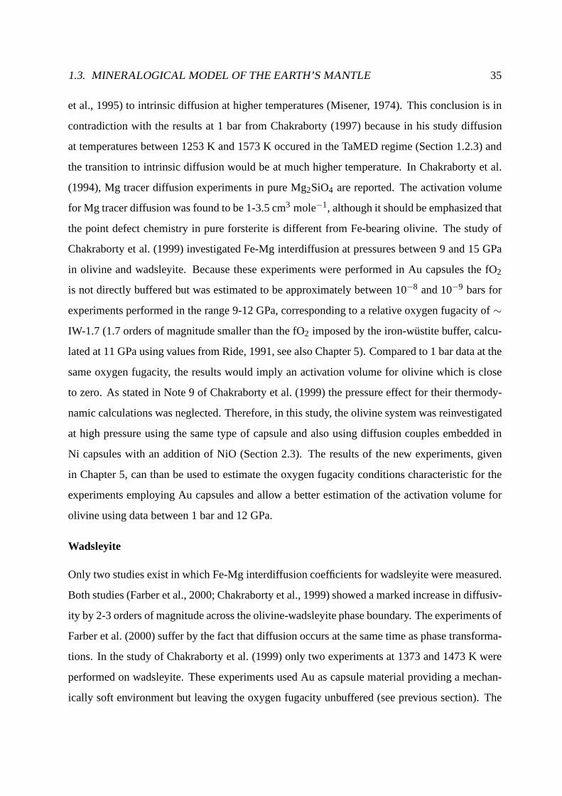
1.3. MINERALOGICAL MODEL OF THE EARTH’S MANTLE 35
et al., 1995) to intrinsic diffusion at higher temperatures(Misener, 1974). This conclusion is in
contradiction with the results at 1 bar from Chakraborty (1997) because in his study diffusion
at temperatures between 1253 K and 1573 K occured in the TaMEDregime (Section 1.2.3) and
the transition to intrinsic diffusion would be at much higher temperature. In Chakraborty et al.
(1994), Mg tracer diffusion experiments in pure Mg2SiO4 are reported. The activation volume
for Mg tracer diffusion was found to be 1-3.5 cm3 mole−1, although it should be emphasized that
the point defect chemistry in pure forsterite is different from Fe-bearing olivine. The study of
Chakraborty et al. (1999) investigated Fe-Mg interdiffusion at pressures between 9 and 15 GPa
in olivine and wadsleyite. Because these experiments were performed in Au capsules the fO2
is not directly buffered but was estimated to be approximately between 10−8 and 10−9 bars for
experiments performed in the range 9-12 GPa, correspondingto a relative oxygen fugacity of∼IW-1.7 (1.7 orders of magnitude smaller than the fO2 imposed by the iron-wustite buffer, calcu-
lated at 11 GPa using values from Ride, 1991, see also Chapter5). Compared to 1 bar data at the
same oxygen fugacity, the results would imply an activationvolume for olivine which is close
to zero. As stated in Note 9 of Chakraborty et al. (1999) the pressure effect for their thermody-
namic calculations was neglected. Therefore, in this study, the olivine system was reinvestigated
at high pressure using the same type of capsule and also usingdiffusion couples embedded in
Ni capsules with an addition of NiO (Section 2.3). The results of the new experiments, given
in Chapter 5, can than be used to estimate the oxygen fugacityconditions characteristic for the
experiments employing Au capsules and allow a better estimation of the activation volume for
olivine using data between 1 bar and 12 GPa.
Wadsleyite
Only two studies exist in which Fe-Mg interdiffusion coefficients for wadsleyite were measured.
Both studies (Farber et al., 2000; Chakraborty et al., 1999)showed a marked increase in diffusiv-
ity by 2-3 orders of magnitude across the olivine-wadsleyite phase boundary. The experiments of
Farber et al. (2000) suffer by the fact that diffusion occursat the same time as phase transforma-
tions. In the study of Chakraborty et al. (1999) only two experiments at 1373 and 1473 K were
performed on wadsleyite. These experiments used Au as capsule material providing a mechan-
ically soft environment but leaving the oxygen fugacity unbuffered (see previous section). The

36 CHAPTER 1. INTRODUCTION
calibration of the fO2 conditions inside the Au capsules, as outlined above for olivine, also helps
in constraining the oxygen fugacity conditions in the experiments of Chakraborty et al. (1999)
for wadsleyite. In this study experiments at higher temperatures than used by Chakraborty et al.
(1999) were performed and the results are compared with their data in order to obtain a better
estimate of the activation energy for diffusion in wadsleyite (section 5.3).
Ferropericlase
Most studies of diffusion in the system MgO-FeO have been performed on the end member
MgO. Reviews of Mg and O self-diffusion data at 1 bar and variable temperatures can be found
in Freer (1980) and Wuensch (1983). Vocadlo et al. (1995) investigated ionic diffusion in MgO
by computer calculations via lattice dynamics.
Fe tracer diffusion experiments in (Mg,Fe)O solid solutions were performed by Chen and Pe-
terson (1980). The oxygen fugacity dependence follows the ideal f O1/62 -dependence (Equation
1.10) and the Fe tracer diffusion coefficient depends exponentially on composition. Only a few
studies exist on Fe-Mg interdiffusion in the system MgO-FeO. Experiments employing polycrys-
talline diffusion couples or single crystals embedded in powders were performed by Bygden et al.
(1997), Rigby and Cutler (1965) and Blank and Pask (1969). The temperature range of these ex-
periments was restricted to 1363 - 1588 K. The oxygen fugacity was not buffered directly and
led to discrepancies in the results (see Bygden et al. (1997) for a discussion and comparison of
results).
Mackwell et al. (2004, in preparation) performed Fe-Mg interdiffusion experiments employ-
ing single crystal diffusion couples over a wide range of temperatures and oxygen fugacities at 1
bar. According to their results, diffusion depends on oxygen fugacity with an exponent of 0.22,
slightly different from the ideal value 1/6 in Eq. 1.10, and depends exponentially on composition,
and the interdiffusion coefficient is given by:
DFe−Mg = (D01+D02 · f O2m ·XFeO
p) ·exp
(
−EA−α ·XFeO
R·T
)
(1.16)
whereD01 = 1.8× 10⁻⁸ m2 sec−1, D02 = 1.1× 10⁻⁴ m2 sec−1, the activation energyEA =
206500 J mol−1, α = 61950 J mol−1, m= 0.22, p = 1.17, R is the molar gas constant, andT
is temperature. This equation was derived by Mackwell et al.(2004, in preparation) using point

1.3. MINERALOGICAL MODEL OF THE EARTH’S MANTLE 37
defect arguments and the values of its parameters are best fitvalues to their data. The power law
dependence only plays a significant role at low iron concentrations, whereas for compositions
with XFeO > 0.07, diffusivities are primarily exponentially dependent on composition; Eq. 1.16
can than be approximated at constant temperature by:
D = D0 ·exp(a ·c(x)) (1.17)
where the constanta controls the extent of asymmetry observed in the diffusion profiles and the
preexponential factor includes the temperature and oxygenfugacity of the experiment which are
constant for each individual experiment. A pure exponential compositional dependence was ob-
served for Fe-Mg interdiffusion in ferropericlase by Bygd´en et al. (1997), for Ni tracer diffusion
from thin films into NiO-MgO single crystal solid solutions by Wei and Wuensch (1973) and in
interdiffusion studies of NiO-MgO by Blank and Pask (1969),Appel and Pask (1971), and Jakob-
sson (1996). Also for olivine (Morioka and Nagasawa, 1991) apure exponential dependence on
composition was observed.
To understand transport processes in the lower mantle, where ferropericlase is an important
constituent phase, diffusivities as a function of pressureare needed. (FexMg1−x)O ferropericlase
is well suited for high pressure experiments due to the largestability field of this phase. Ita and
Cohen (1997, 1998) performed a theoretical study on diffusion in pure MgO at high pressures.
Calculated self-diffusion coefficients for Mg and O decrease with increasing pressure. Van Or-
man et al. (2003) performed multi-anvil experiments to measure Mg, Al and O self-diffusion in
MgO between 15 and 25 GPa at a constant temperature of 2273 K. Their results agree with the
theoretical work of Ita and Cohen (1998) and the experimentally determined activation volume
for Mg diffusion is 3.0 cm3/mole.
Yamazaki and Irifune (2003) recently determined Fe-Mg interdiffusion coefficients for fer-
ropericlase. They derived an activation volume of 1.8 cm3 mol−1 and an activation energy of 226
kJ mol−1. The experiments were conducted mostly in Re capsules (P< 30 GPa). In addition at
35 GPa a graphite capsule experiment was performed. Although it is assumed that the experi-
ments follow a trend compatible with the Re-ReO2 buffer this assumption was not tested and the
results are therefore unconstrained with respect to oxygenfugacity.
38 CHAPTER 1. INTRODUCTION
Silicate perovskite
In spite of the fact that (Mg,Fe)SiO3 is believed to be the most abundant mineral in the Earth
there is an overall lack of experimental Fe-Mg interdiffusion studies for this mineral.
Computer simulations were performed by Wright and Price (1993) using an ab initio atom-
istic simulation. The calculated activation enthalpy for intrinsic Si diffusion is so high (Ha =
1113 kJ mol−1) that these authors conclude that Si diffusion in the lattice most likely occurs by
an extrinsic process. For Mg an extrinsic activation enthalpy of 440.6 kJ mol−1 at 0 GPa and
717.0 kJ mol−1 at 125 GPa was derived. For the pressure effect of diffusion,activation volumes
of 2.1 and 4.96 cm3 mol−1 for extrinsic and intrinsic Mg diffusion respectively werederived,
whereas for Si a negative activation volume for extrinsic diffusion was found implying that Mg
becomes the slowest diffusing species in the deeper parts ofthe lower mantle.
The only experimental study performed so far was a study of silicon self-diffusion in pure
MgSiO3 by Yamazaki et al. (2000). These authors measured lattice and grain boundary diffusion
coefficients (Dl andDgb) and give for both types of diffusion an Arrhenius relationship:
Dl (m2 sec−1) = 2.74×10⁻¹⁰exp
(−336(kJ mol−1)
RT
)
(1.18)
δDgb (m3 sec−1) = 7.12×10⁻¹⁷exp
(−311(kJ mol−1)
RT
)
(1.19)
whereδ denotes effective grain boundary width, R is the gas constant, andT is temperature.
1.4 Aims of the present study
In order to have a better understanding of kinetic processesoccurring in the Earth (Section 1.1),
experimental diffusion studies in a multianvil apparatus were performed
• to investigate the whole pressure stability range of olivine for a better constraint of the
activation volume for Fe-Mg interdiffusion and Mn and Ni diffusion,
• to determine the activation energy for Fe-Mg interdiffusion in olivine at pressures close to
the stability limit,
• to constrain the activation energy of Fe-Mg interdiffusionin wadsleyite,

1.4. AIMS OF THE PRESENT STUDY 39
• to establish a database of Fe-Mg interdiffusion in ferropericlase at pressures between 6
and 23 GPa and temperatures between 1653 and 2073 K at controlled oxygen fugacity
conditions,
• to derive for the first time Fe-Mg interdiffusion coefficients in (Mg,Fe)SiO3 perovskite, the
most abundant mineral of our planet.

40 CHAPTER 1. INTRODUCTION
Chapter 2
Experimental Techniques
2.1 Introduction
For the determination of Fe-Mg interdiffusion coefficientsin olivine, wadsleyite, ferropericlase
and silicate perovskite, diffusion couple experiments were performed at high pressure in a mul-
tianvil apparatus. For diffusion studies, diffusion couples should have sample sizes of at least
∼ 250 µm diameter and∼ 100 µm thickness, otherwise handling of the samples becomes ex-
tremely difficult. Therefore, the multianvil appartus is the most suitable technique for studying
the pressure range of 6-26 GPa, investigated in this study, because samples with volumes of 1
mm3 can be easily accomodated. The upper pressure limit that canbe reached with this tech-
nique, employing sintered WC cubes as pressure transmitting medium, is about 27 GPa. With
sintered diamond cubes the pressure range can be extended toabout 40 GPa (Irifune et al., 2002).
Although the diamond anvil cell (DAC) can provide much higher pressures, equivalent to the
whole pressure range of the lower mantle (23 - 137 GPa) and to core conditions (136-360 GPa),
the sample volume is in general to small for diffusion coupleexperiments (for a description of
the DAC see e.g. Eremets, 1996). In addition, temperature gradients in laser heated DAC are to
high for precise diffusion coefficient determinations because of the strong dependence of diffu-
sivity on temperature (Section 1.2.5). In this chapter, after explaining the basics of the multianvil
technique (Section 2.2), the setup and the compositions of the diffusion couples for the different
mineral systems are described (Section 2.3). For high pressure experiments a suitable capsule
material has to be selected that does not destabilize the sample and provides a mechanically
suitable (low stress) environment. The choice for capsule materials employed in this study is
41

42 CHAPTER 2. EXPERIMENTAL TECHNIQUES
outlined in Section 2.4. Section 2.5 describes the assemblies used for the high pressure diffusion
experiments.
2.2 High pressure experiments: Multi anvil technique
The multianvil technique is described in detail in a number of publications (Kawai and Endo,
1970; Kawai et al., 1973; Spain and Paauwe, 1977a; Graham, 1987; Ohtani et al., 1987; Walker
et al., 1990; Liebermann and Wang, 1992; Rubie et al., 1993; Rubie, 1999; Irifune, 2002).
The principles of the multianvil apparatus are shown schematically in Figure 2.1. The force
of a hydraulic press is exerted onto a set of 6 steel anvils that form a cubic gap filled with 8 WC
cubes. Because the corners of the WC cubes are truncated, they form an octahedral pressure
chamber, which is filled by an MgO octahedron containing the sample capsule. All presses
installed at the Bayerisches Geoinstut with axial forces between 500 and 5000 t were used for
performing experiments in this study (Table A.1). More details of the technique are given in
Appendix A.
The maximum pressure that can be reached in an experiment depends on the force applied,
the edge length of the octahedron and the truncantion edge length of the cubes. For synthe-
sis, experiments have been performed to produce starting samples of the high pressure phases
wadsleyite and (Mg,Fe)SiO3 perovskite (see Section 2.3 for details) employing 14/8 and10/4
assemblies where the first number is the octahedron edge length and the second number is the
truncation edge length. A schematic drawing of the synthesis assemblies is shown in Figure 2.2.
Because of the wide range of pressures covered for diffusionexperiments in this study, a large
variety of assemblies were employed, to accomodate the diffusion couples, by modifying the
standard assemblies used at the Bayerischen Geoinstitut. The details of these assemblies are ex-
plained in Section 2.5 after a description of diffusion couples (Section 2.3) and sample capsules
(Section 2.4).
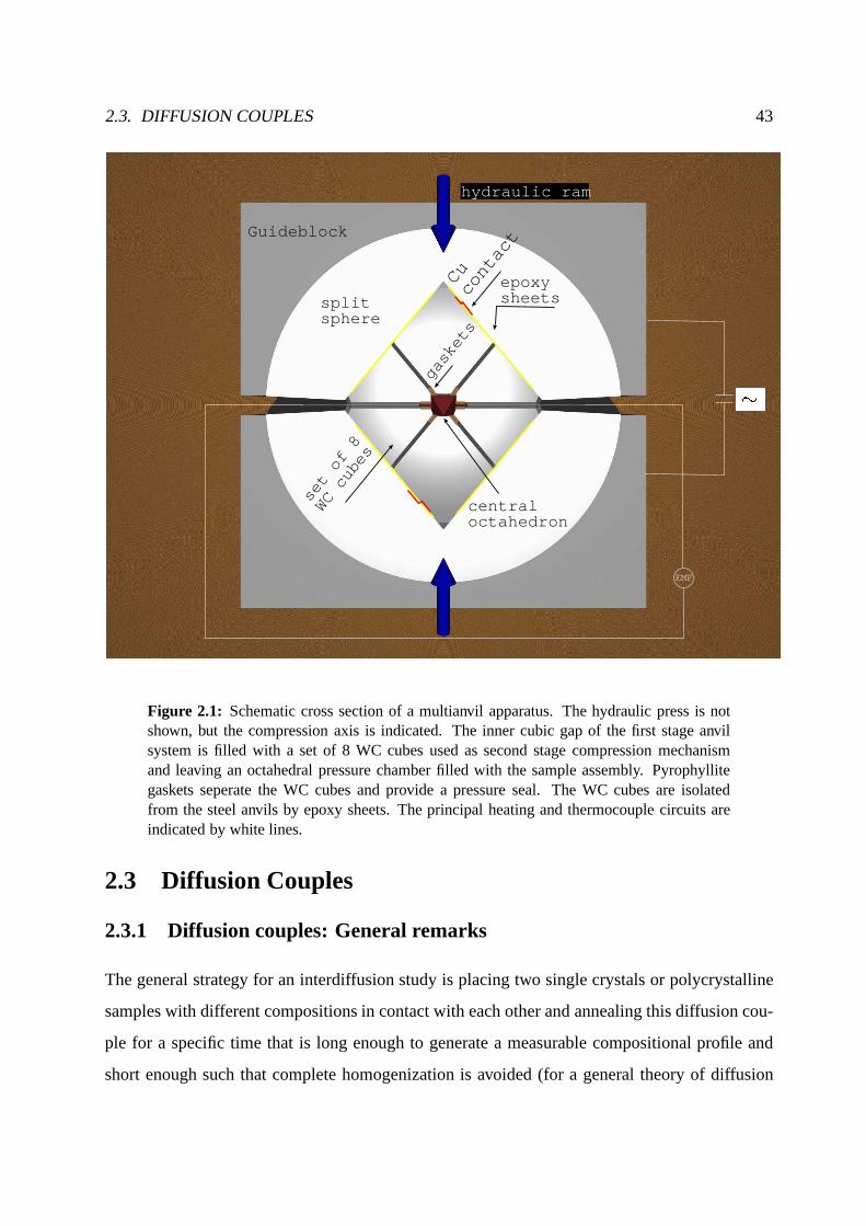
2.3. DIFFUSION COUPLES 43
EMF
Guideblock
splitsphere
set of 8
WC cubes
epoxysheets
Cucontact
gaskets
centraloctahedron
hydraulic ram
Figure 2.1: Schematic cross section of a multianvil apparatus. The hydraulic press is notshown, but the compression axis is indicated. The inner cubic gap of the first stage anvilsystem is filled with a set of 8 WC cubes used as second stage compression mechanismand leaving an octahedral pressure chamber filled with the sample assembly. Pyrophyllitegaskets seperate the WC cubes and provide a pressure seal. The WC cubes are isolatedfrom the steel anvils by epoxy sheets. The principal heatingand thermocouple circuits areindicated by white lines.
2.3 Diffusion Couples
2.3.1 Diffusion couples: General remarks
The general strategy for an interdiffusion study is placingtwo single crystals or polycrystalline
samples with different compositions in contact with each other and annealing this diffusion cou-
ple for a specific time that is long enough to generate a measurable compositional profile and
short enough such that complete homogenization is avoided (for a general theory of diffusion
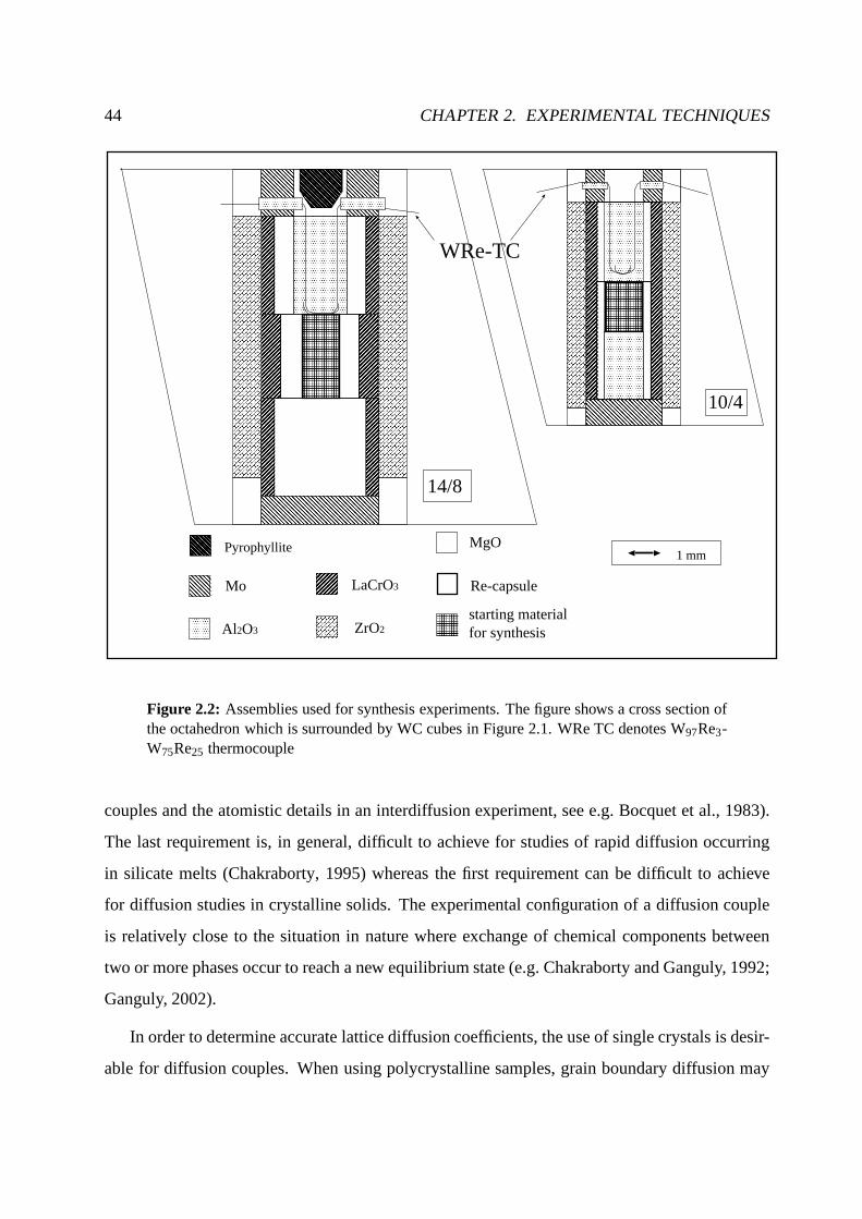
44 CHAPTER 2. EXPERIMENTAL TECHNIQUES
Mo
Al2O3
LaCrO3
ZrO2
MgO
Re-capsule
starting materialfor synthesis
WRe-TC
1 mm
14/8
10/4
Pyrophyllite
Figure 2.2: Assemblies used for synthesis experiments. The figure showsa cross section ofthe octahedron which is surrounded by WC cubes in Figure 2.1.WRe TC denotes W97Re3-W75Re25 thermocouple
couples and the atomistic details in an interdiffusion experiment, see e.g. Bocquet et al., 1983).
The last requirement is, in general, difficult to achieve forstudies of rapid diffusion occurring
in silicate melts (Chakraborty, 1995) whereas the first requirement can be difficult to achieve
for diffusion studies in crystalline solids. The experimental configuration of a diffusion couple
is relatively close to the situation in nature where exchange of chemical components between
two or more phases occur to reach a new equilibrium state (e.g. Chakraborty and Ganguly, 1992;
Ganguly, 2002).
In order to determine accurate lattice diffusion coefficients, the use of single crystals is desir-
able for diffusion couples. When using polycrystalline samples, grain boundary diffusion may

2.3. DIFFUSION COUPLES 45
also occur and either the experimental setup should allow for separation of the two effects or
bulk diffusion should be the dominant process (for the theory of grain boundary diffusion see
Herzig and Mishin, 1998). The last case is generally true forlarge grain sizes and high tempera-
tures. In this study, single crystals were used in studies ofolivine and ferropericlase, whereas for
wadsleyite and perovskite, polycrystalline starting materials were synthesized prior to diffusion
runs
The analysis of diffusion profiles after the diffusion experiments is described in Chapter 3
and the mathematical treatment of the diffusion profiles is described in Chapter 4.
2.3.2 Diffusion couples: Olivine
All olivine diffusion experiments utilized samples from the same two single crystals as starting
materials. One endmember was synthetic pure Mg2SiO4, forsterite, grown by the Czochralski
method by H. Takei at Tohoku University. It is the same crystal (called Fo1) used by Chakraborty
et al. (1994), where also trace element contents are given. The Fe content of this crystal is be-
tween 122 and 180 ppm. The Fe-bearing endmember was a naturalsingle crystal from San Carlos
with an average Mg-value Mg/(Mg+Fe) = 0.94 with 3000 ppm NiO and 1500 ppm MnO. Both
crystals were oriented along the crystallographic c-direction by Laue backscatter diffraction such
that the c axis is perpendicular to the diffusion interface.After the diffusion experiments the ori-
entation of the two crystals was redetermined by electron backscatter diffraction (EBSD). The
c-axes for both crystals were found in the diffusion plane perpendicular to the diffusion interface
with an error of less than 4◦.
For preparation of the diffusion couples the crystals were cut into polished thin slices with
a thickness of∼ 250µm. Discs were drilled out with a diameter of 250µm (Au-capsule exper-
iments) or 950µm (Ni-NiO capsules). Polishing of the olivine slices (and wadsleyite as well)
was performed with diamond spray (Struers) down to 0.25 microns. The two polished sides were
then placed together and inserted into the capsule (see Section 2.4).

46 CHAPTER 2. EXPERIMENTAL TECHNIQUES
2.3.3 Diffusion couples: Wadsleyite
Wadsleyite diffusion couple experiments employing a single crystal as one endmember are de-
scribed by Chakraborty et al. (1999), but the synthesis of crystals large enough for this study
failed. Thus, polycrystalline wadsleyite samples were synthesized prior to diffusion runs as
starting material. For all synthesis experiments a 14/8 assembly was used (for a description
of the high pressure assemblies see Section 2.5). A polycrystalline pure Mg2SiO4 wadsleyite
sample was prepared by annealing forsterite powder at 15 GPaand 1673 K in a 1000 t multi-
anvil press employing a Re-foil capsule (Section 2.4). The powder with forsterite composition
was kindly provided by D.J. Frost. For the Fe-bearing sample, a single crystal of olivine with
Fe/(Mg+Fe) = 0.84 from San Carlos, kindly provided by S. Mackwell, was used.The conver-
sion from olivine to wadsleyite was performed at 15 GPa and 1873 K, using a capsule prepared
of Re-foil. Another Fe-bearing wadsleyite sample was synthesized from hot-pressed San Carlos
olivine powder at 15 GPa and 1673 K in a Re-capsule. To confirm that the synthesized samples
consisted of wadsleyite, the material was characterized byRaman spectroscopy (Fig. 2.3) using
a LabRAM microraman instrument (Jobin Yvon GmbH). X-ray microdiffraction patterns could
be easily indexed with the reference pattern of Moore and Smith (1970). The X-ray diffraction
pattern contained only peaks that are attributable to wadsleyite. Unfortunately Moore and Smith
(1970) only collected data for the interplanar spacingdobs in the range 6.69> dobs > 0.9156.
Therefore assignment for low d-spacings (largeθ) was not possible.
After synthesis the samples were removed from the high pressure assembly and the Re foil
was withdrawn. Subsequently they were cut into discs∼ 250µm thick and mounted on glass
slides to enable them to be polished in the same way as the olivine samples. After polishing,
small discs were drilled out for use in diffusion couples as already described for olivine (Section
2.3.2).
2.3.4 Diffusion couples: Ferropericlase
Two ferropericlase single crystal slices (500µm thick) were obtained from S. Mackwell. They
had been synthesized by embedding a slice of a pure syntheticsingle crystal of MgO in (Mg,Fe)O
powder and annealing at controlled oxygen fugacity (Holzapfel et al., 2003). The resulting nom-

2.3. DIFFUSION COUPLES 47
400 500 600 700 800 900 1000
Inte
nsity
, a.u
.
Wavenumber, cm-1
San Carlos, Mg90San Carlos, Mg84
Figure 2.3: Raman spectra used to identify the (Mg,Fe)2SiO4 phases produced in synthe-sis experiments for wadsleyite. Representative spectra from synthesis experiments per-formed at 15 GPa, 1873 K (Fo84) and 1673 K (Fo90) are shown. The Raman pat-terns can be identified as wadsleyite by comparing them to Raman patterns of wads-leyite and ringwoodite given in Figure 1 in McMillan and Akaogi (1987) and of forsteriteusing data from the web-based database of the California Institute of Technology athttp://minerals.gps.caltech.edu/FILES/raman/Caltechdata.
inal compositions wereXFeO = 0.07 andXFeO = 0.35, whereXFeO is mole fraction of FeO. The
diffusion interface was polished with alumina powders to 0.3 microns. For the high-pressure
diffusion experiments, discs 1 mm in diameter and 500µm thick were drilled out as starting
crystals. Electron microprobe traverses over the samples showed heterogeneities of less than±1.5 mole% FeO along the entire length of the crystal and less than± 0.25 mole% over the 1 mm
diameter of the diffusion couples. On one side of the low ironcontent crystal a well sintered layer
with polycrystalline (Mg,Fe)O with the same composition and a Ca2SiO4 phase was observed
after the experiments, possibly due to contamination during sample preparation.

48 CHAPTER 2. EXPERIMENTAL TECHNIQUES
2.3.5 Diffusion couples: (Mg,Fe)SiO3 perovskite
Samples for diffusion runs were synthesized in Re-capsules, employing a 10/4 assembly (Figure
2.2), at 2073 K and 25 GPa using synthetic MgSiO3 powder, (Mg,Fe)SiO3 powder with vary-
ing Fe/Fe+Mg (kindly provided by D.J. Frost) and a single crystal of natural pyroxene (kindly
provided by S. Mackwell) withXFeSiO3 = 0.136. The pyroxene contains only trace amounts of
aluminium and Calcium (850 ppm Al2O3 and 2200 ppm CaO), hence all compositions of the
perovskite diffusion couples are restricted to the MgSiO3-FeSiO3 binary system.
The phase identity of the synthesis runs were checked by Raman spectroscopy. Typical spec-
tra obtained by a Raman microscope are shown in Fig. 2.4. For Fe-bearing perovskite two rela-
tively broad peaks occur at 727 and 894 wavenumbers. These are typical for samples containing
Fe (C. Liebske and L. Dubrovinsky, pers. communication) andare probably attributable to a
second order Raman effect due to disorder in the perovskite structure similar to that occurring in
manganites or rare earth element perovskites (Dubrovinsky, pers. communication).
After the synthesis the samples were removed from the assembly and the Re-foil capsule,
cut into discs∼ 100µmthick and mechanically polished. Because perovskites are unstable with
respect to mechanical preparation, in addition to mechanical polishing, chemical polishing with
a colloidal silica suspension (OP-S or OP-U suspension obtained from Struers A/S) was also
performed. To test the crystallinity of the polished surfaces, orientation contrast imaging and
electron backscatter diffraction (EBSD) were carried out using a LEO Gemini 1530 scanning
electron microscope (SEM) equipped with a field emission gun(FEG). Both methods are based
on scattering of electrons in the surface and hence can be used as a probe for surface crystallinity.
Figure 2.5 shows an orientation contrast image of a pure MgSiO3 sample. The orientation con-
trast observed, reveals the good crystallinity of the samples. If the area of observation is reduced
significantly the surface becomes damaged by the electron beam and the orientation contrast
quickly degrades. Yamazaki et al. (2000) reported that theyobserved EBSD patterns for their
pure MgSiO3 perovskite samples used to study Si self-diffusion although no example is given in
their work. For the samples of this study very weak EBSD patterns only appeared for a very short
time when scanning over a big crystal grain. A focused electron beam immediately destroys the
surface of the crystal and no EBSD pattern can be obtained.

2.3. DIFFUSION COUPLES 49
200 400 600 800 1000 1200
Inte
nsity
, a.u
.
Raman shift, cm-1
MgSiO3 perovskite:
(Mg,Fe)SiO3 perovskite:
Figure 2.4: Typical Raman spectra from different synthesis runs. For Fe-bearing perovskitetwo broad bands appear at approximately 727 and 894 wavenumbers (see text for explana-tion).

50 CHAPTER 2. EXPERIMENTAL TECHNIQUES
30 µm
Figure 2.5: Orientation contrast image of a MgSiO3 perovskite synthesized at 2073 K and 25GPa for 2 hours. Ubiquitous twinning can be observed. The role of twinning and structuralphase transitions is discussed in Sections 1.3.1 and 5.5.2
2.4 Capsules
Requirements for capsule materials
In previous studies of diffusion at high pressure several different capsule materials were em-
ployed (Bejina et al., 2003). The ideal capsule material does not interact chemically with the
sample (for example no Fe loss), buffers the oxygen fugacityand is mechanically weak and
thus provides a hydrostatic environment to minimize differential stresses imposed on the diffu-
sion couple. It is difficult to meet all these requirements atthe same time with any one capsule
type. Therefore, different capsule materials were used in this study. For most off the olivine
experiments, mechanically weak Au capsules were employed,as described in Chakraborty et al.
(1999). To calibrate the oxygen fugacity conditions in the Au capsules some experiments were
also performed using Ni capsules with added NiO. The addition of NiO buffers thef O2 at the
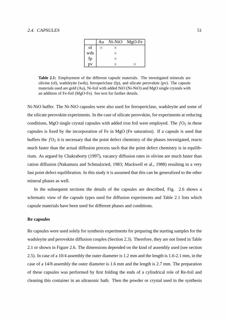
2.4. CAPSULES 51
Au Ni-NiO MgO-Feol × ×
wds ×fp ×pv × ×
Table 2.1: Employment of the different capsule materials. The investigated minerals areolivine (ol), wadsleyite (wds), ferropericlase (fp), and silicate perovskite (pv). The capsulematerials used are gold (Au), Ni-foil with added NiO (Ni-NiO) and MgO single crystals withan addition of Fe-foil (MgO-Fe). See text for further details.
Ni-NiO buffer. The Ni-NiO capsules were also used for ferropericlase, wadsleyite and some of
the silicate perovskite experiments. In the case of silicate perovskite, for experiments at reducing
conditions, MgO single crystal capsules with added iron foil were employed. Thef O2 in these
capsules is fixed by the incorporation of Fe in MgO (Fe saturation). If a capsule is used that
buffers thef O2 it is necessary that the point defect chemistry of the phasesinvestigated, reacts
much faster than the actual diffusion process such that the point defect chemistry is in equilib-
rium. As argued by Chakraborty (1997), vacancy diffusion rates in olivine are much faster than
cation diffusion (Nakamura and Schmalzried, 1983; Mackwell et al., 1988) resulting in a very
fast point defect equilibration. In this study it is assumedthat this can be generalized to the other
mineral phases as well.
In the subsequent sections the details of the capsules are described, Fig. 2.6 shows a
schematic view of the capsule types used for diffusion experiments and Table 2.1 lists which
capsule materials have been used for different phases and conditions.
Re capsules
Re capsules were used solely for synthesis experiments for preparing the starting samples for the
wadsleyite and perovskite diffusion couples (Section 2.3). Therefore, they are not listed in Table
2.1 or shown in Figure 2.6. The dimensions depended on the kind of assembly used (see section
2.5). In case of a 10/4 assembly the outer diameter is 1.2 mm and the length is 1.6-2.1 mm, in the
case of a 14/8 assembly the outer diameter is 1.6 mm and the length is 2.7 mm. The preparation
of these capsules was performed by first folding the ends of a cylindrical role of Re-foil and
cleaning this container in an ultrasonic bath. Then the powder or crystal used in the synthesis

52 CHAPTER 2. EXPERIMENTAL TECHNIQUES
-�1 mm
Au
DC
pppppppppppppppppppppppppppppppppppppppppppppppppppppppppppppppppppppppppppppppppppppppppppppppppppppppppppppppppppppppppppppppppppppppppppppppppppppppppppppppppppppppppppppppppppppppppppppppppppppppppppppppppppppppppppppppppppppppppppppppppppppppppppppppppppppppppppppppppppppppppppppppppppppppppppppppppppppppppppppppppppppppppppppppppppppppppppppppppppppppppppppppppppppppppppppppppppppppppppppppppppppppppppppppppppppppppppppppppppppppppppppppppppppppppppppppppppppppppppppppp
Ni
NiO
DC
S-XX MgO
6
Fe foil
DC
S-XX MgO
?
P-XX MgO
A B C
Figure 2.6: Graphical representation of the three different capsule types used for high pres-sure diffusion runs. A: Au capsule, B: Ni-NiO capsule, C: MgO-Fe capsule. P-XX denotespolycrystalline. S-XX denotes single crystal, and DC denotes diffusion couple.
run is added and in case of the powder slightly compressed with a steel rod. Subsequently the
capsule is closed by folding the surmounting ends over and gently pressing it together.
Au capsules
For preparation of the capsules a Au wire of 1mm diameter was drilled with a hole of 250µm
diameter. Discs of the single crystals of olivine (see Section 2.3.2) were carefully inserted and
the capsule closed. Figure 2.6 shows the capsule schematically. After insertion of the diffusion
couple the sample was closed by deformation of the soft capsule (Chakraborty et al., 1999).
MgO-Fe capsules
This capsule type was used solely for a set of experiments on silicate perovskite. A cylinder was
drilled out of a commercially available single crystal of MgO with a diameter of 1.5 mm. Into the
cylinder an inner hole was drilled with a diameter of 1.0 mm. Into the bottom of the inner hole

2.5. ASSEMBLIES USED FOR HIGH PRESSURE DIFFUSION EXPERIMENTS 53
an Fe disc was inserted on top of which the two slices of polycrystalline perovskite were placed.
Another single crystal MgO disc was added to be able to study interaction of Fe with MgO as
well, and then the rest of the capsule was filled with a polycrystalline MgO disc. The reducing
conditions of this capsule type imposed by the Fe-distribution between Fe-metal and (Mg,Fe)O,
formed on the rim of the capsule, should mimic oxygen fugacity conditions prevailing during
core formation and at the present-day core-mantle boundary.
Ni-NiO capsules
This capsule type was used for all phases investigated in this study (Table 2.1). The Ni cap-
sules were prepared by rolling Ni-foil (thickness 125µm,, 99.98%, Goodfellow) into a cylinder
and folding one end over to form the bottom of the capsule. Thetwo polycrystalline slices of
wadsleyite or perovskite or single crystals of olivine or ferropericlase were inserted such that the
polished sides were together. NiO powder was added on top of the diffusion couple. The NiO
powder was previously dried at 1273 K in an Al2O3-crucible to prevent water contamination. At
these conditions the crucible did not react with the powder to form Ni-Al spinel as confirmed
by microprobe analysis. The capsule was subsequently closed by folding the end of the foil and
gently uniaxially compressing the capsule.
In this kind of capsule the oxygen fugacity should be close tothe Ni-NiO buffer system.
Ni+NiO was also used in the experiments of Farber et al. (2000) to buffer oxygen fugacity.
These authors claim that the SiO2-activity was buffered by the equilibrium of NiO and Ni2SiO4,
which was also present in their experiments. By a similar reasoning silica activity in this study
should be controlled in the case of olivine by formation of a Ni2SiO4 component due to Mg-Ni
exchange at the NiO-olivine interface and subsequent SiO2 buffering due to the equilibrium of
Ni-metal and Ni2SiO4 dissolved in olivine.
2.5 Assemblies used for high pressure diffusion experiments
For experiments at pressures between 6 and 15 GPa a 14/8 type multianvil assembly and for
pressures between 15 and 26 GPa a 10/4 type multianvil assembly were used. In the 5000 t press
(Zwick, Table A.1), where sample volumes are significantly larger, an 18/8 multianvil assembly

54 CHAPTER 2. EXPERIMENTAL TECHNIQUES
14/8 10/4 18/8ol 6-12
wds 15fp 8-12 16-23pv 25-26 22
Table 2.2: Range of use of the different octahedral assemblies. The numbers given foreach combination of mineral phase (ol = olivine, wds = wadsleyite, fp = ferropericlase, pv= perovskite) and octahedral assembly (see text for explanation of assembly abbreviations)denote investigated pressure range in GPa.
could be employed for two silicate perovskite diffusion experiments at pressures of 22 GPa.
Table 2.2 shows the assemblies used and the pressure range attained for the different minerals
investigated in this study. For a detailed description of multianvil assemblies see also Liebermann
and Wang (1992), Walter et al. (1995), and Rubie (1999).
Fig. 2.7-2.9 show the details of the multianvil assemblies for the different phases investi-
gated. The details are described in Appendix A. The 10/4 assembly employs a straight LaCrO3
resistance heater where temperature gradients can be as high as 100 K/mm (Trønnes, 2000),
whereas all other assemblies use a stepped LaCrO3 heater greatly reducing temperature gradi-
ents (Rubie et al., 1993). In all cases a W97Re3-W75Re25 thermocouple was used and tempera-
ture was not corrected for the pressure effect on the electromotive force (for a discussion of the
maximum error involved, see Appendix A).
For pressure calibration, known phase transition points are employed in order to calibrate
the oil pressure of the hydraulic system against the pressure acting on the sample. For the 14/8
assembly (olivine, ferropericlase and wadsleyite experiments) the coesite⇀↽ stishovite (Zhang
et al., 1996) and the Mg2SiO4 α ⇀↽ β (Morishima et al., 1994) phase transformations at 1473 K
were employed. The calibration for the 10/4 assembly (ferropericlase, (Mg,Fe)SiO3 perovskite
experiments) was based on the phase boundaries ofγ ⇀↽ perovskite+MgO, β ⇀↽ γ, andα ⇀↽ β
in Mg2SiO4 (Akaogi et al., 1989; Morishima et al., 1994; Suzuki et al., 2000) as well as the
ilmentite⇀↽ perovskite phase boundary in the system MgSiO3 (Ono et al., 2001). For the 18/8
assembly the Mg2SiO4 α ⇀↽ β, the Mg2SiO4 β ⇀↽ γ phase boundaries both at 1673 K (Morishima
et al., 1994), with the additional constraint of an unbracketed occurence of MgSiO3 perovskite
at 2273 K were used.
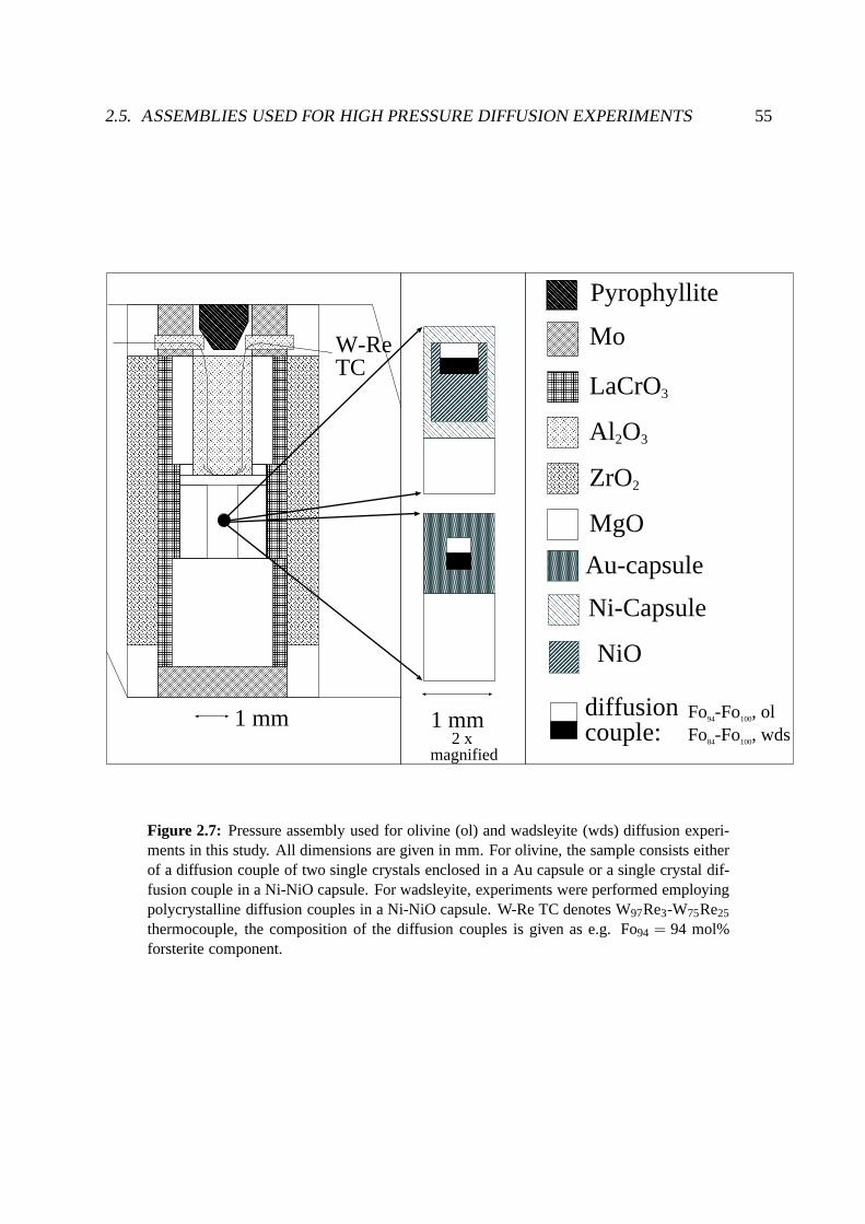
2.5. ASSEMBLIES USED FOR HIGH PRESSURE DIFFUSION EXPERIMENTS 55
W-ReTC
1 mm 1 mm
LaCrO3
Al 2O3
ZrO2
MgO
Au-capsule
diffusion couple:
Fo94-Fo100, olFo84-Fo100, wds
Mo
Pyrophyllite
Ni-Capsule
NiO
2 x magnified
Figure 2.7: Pressure assembly used for olivine (ol) and wadsleyite (wds) diffusion experi-ments in this study. All dimensions are given in mm. For olivine, the sample consists eitherof a diffusion couple of two single crystals enclosed in a Au capsule or a single crystal dif-fusion couple in a Ni-NiO capsule. For wadsleyite, experiments were performed employingpolycrystalline diffusion couples in a Ni-NiO capsule. W-Re TC denotes W97Re3-W75Re25
thermocouple, the composition of the diffusion couples is given as e.g. Fo94 = 94 mol%forsterite component.

56 CHAPTER 2. EXPERIMENTAL TECHNIQUES
Mo
Al 2O3
LaCrO3
ZrO2
MgO
Ni-capsule
NiO
(Mg0.93Fe0.07)O-(Mg0.63Fe0.37)Odiffusion couple
thermocouple
1 mm
14/8
10/4
Pyrophyllite
Figure 2.8: Pressure assemblies for multianvil experiments used in this study for ferroper-iclase. At P< 16 GPa a 14/8 assembly (14 mm edge length of the octahedron, WCcubeswith 8 mm edge length corner truncations) and at P≥ 16 GPa a 10/4 assembly were used.The sample capsule consists of Ni foil with the addition of NiO to buffer fO2

2.5. ASSEMBLIES USED FOR HIGH PRESSURE DIFFUSION EXPERIMENTS 57
TC
10/4
18/8
2.0 mm
Mo
MgO-Sgl-XXLaCrO3
Al 2O3
ZrO2
MgO
Fe-Pvsk
Mg-Pvsk
Fe-foil
TC
Py
Figure 2.9: Pressure assembly used for perovskite diffusion experiments in this study. An18/8 assembly was employed in a 5000 t press at 22 GPa for temperatures higher than 2273K. For lower temperatures a 10/4 assembly was used at pressures of 25-26 GPa in a 1000 tor 1200 t press. Sgl-XX denotes single crystal, TC denotes W97Re3-W75Re25 thermocouple,and Py denotes pyrophyllite. In addition to MgO-Fe capsulesalso Ni-NiO capsules wereemployed in the 10/4 assembly for some of the experiments, similar to the ferropericlaseexperiments shown in Fig. 2.8.

58 CHAPTER 2. EXPERIMENTAL TECHNIQUES

Chapter 3
Chemical analysis of diffusion profiles
3.1 Choice of analysis techniques
For determining interdiffusion coefficients using the diffusion couple technique, diffusion pro-
files have to be measured with an analytical technique with sufficient precision and lateral reso-
lution. For the purpose of profile analysis, after the annealat high temperatures and pressures,
the sample is cut in a plane perpendicular to the interface toobtain access to the diffusion zone.
In practice, for multianvil experiments, the octahedron ismounted in epoxy resin and polished
until the middle of the diffusion couple is exposed (Figure 3.1).
For measuring the diffusion profiles the samples are first investigated by electron microprobe
analysis (EPMA) . The lateral resolution for a single point analysis is on the order of∼ 2 µm
hence resulting in a minimum profile length of∼ 6 µm (see Section 3.2). For profiles shorter
than the resolution limit of EPMA, the transmission electron microscope (TEM) equipped with
a Ge solid state energy-dispersive X-ray detector (EDX) is used (Section 3.3). This technique
recently became an invaluable tool for studying short diffusion profiles (Meißner et al., 1998). In
addition to the high lateral resolution, on the order of 10 nm, microstructural investigations can
be performed in conjunction with EDX analysis.
For thin film diffusion experiments, used in studies of tracer diffusion, many other analytical
techniques with a very good depth resolution exist, such as secondary ion mass spectrometry
(SIMS), photoelectron spectroscopy, Auger electron spectrometry, Rutherford backscattering, or
nuclear reaction analysis (an overview of these techniqueswith respect to diffusion studies can
be found in Philibert, 1991). These different methods are difficult to apply for diffusion couple
59

60 CHAPTER 3. CHEMICAL ANALYSIS OF DIFFUSION PROFILES
diffusion couple
epoxy block
plane of thin sectionfor TEM analysis
Figure 3.1: After the interdiffusion experiment the octahedron containing the diffusion cou-ple is mounted in epoxy resin and polished down until the diffusion couple is exposed atthe surface (a 10/4 assembly is schematically shown as an example, compare with Fig. 2.8and 2.9). This block is directly used for electron microprobe analysis. For investigationsof short diffusion profiles with a transmission electron microscope a glass slide is glued ontop and the backside of the sample is polished away such that athin slide with a thicknessof ∼ 30 µm remains, which can be further thinned to obtain an electron transparent sample(Section 3.3).
experiments because the diffusion zone can not be investigated in depth mode and the lateral
resolution of the aforementioned techniques often makes them unsuitable.
3.2 Electron microprobe analysis (EPMA)
Reviews about the method can be found in Reed (1975), Heinrich and Newbury (1991), Scott
et al. (1995), or Newbury et al. (1984). During analysis, thesample is subjected to an incident
electron beam. Interactions of the electrons with the atomsin the sample give rise to a number of

3.2. ELECTRON MICROPROBE ANALYSIS (EPMA) 61
secondary signals, among them characteristic X-rays. The X-rays can be detected either with an
energy dispersive or a wavelength dispersive system. The latter method has much better energy
resolution and lower detection limits and is used for quantitative analysis in the case of EPMA,
whereas the TEM used for short profile investigations is equipped with an EDX system (see next
Section).
The lateral resolution depends on the diameter of the interaction volume excited in the sam-
ple. The shape and size of the interaction volume can be modeled by Monte Carlo simulations
(see literature cited in Scott et al., 1995). For operating conditions of 10-20 kV, used in this
study, the smallest diameter of the interaction volume is onthe order of 2µm if the beam is
carefully focused on the sample. The best focus was achievedby aligning the objective aperture
by means of a cathodoluminenscence spot on SnO2. Resolution was optimized by correcting for
astigmatism at high magnifications. With this diameter, profile convolution becomes significant
for a profile length of less then 8µm. The mathematical treatment of deconvolution is evaluated
in Ganguly et al. (1988).
In this work, a Cameca SX-50 equipped with 4 wavelength dispersive spectrometers and a
Jeol JXA 8900 RL at the Institut fur Mineralogie und Geochemie, Universitat zu Koln, equipped
with 5 wavelength dispersive spectrometers, were employed. Tables 3.1 and 3.2 list standards
and measurement conditions for EPMA. Samples were carbon coated (thickness∼ 12 nm) to
avoid charging of the surface. Olivine, wadsleyite, ringwoodite and ferropericlase were studied
at acceleration voltages of either 15 or 20 kV and probe currents between 15 and 20 nA. All
phases are stable at these conditions. On the contrary (Mg,Fe)SiO3 perovskite is very unstable
under the electron beam. To minimize beam damage the probe current was reduced to 5 nA at
15 kV. The clearly visible cathodoluminenscence spot on pure MgSiO3 perovskite decays within
2 sec at these conditions, implying a very fast amorphization.
The detection limits given in Tables 3.1 and 3.2 are calculated by the Cameca software (Ver-
sion 2.15). For major elements, normal working conditions at 15-20 kV and 5-20 nA ensure
sufficient relative precision below∼ 1% at measurement times between 5 and 20 sec (Reed,
1996). Only for the trace elements Ni and Mn in olivine, it wascritical to extent the counting
time to 120 and 150 sec on the peak and 60 and 75 sec on the background, respectively. The

62 CHAPTER 3. CHEMICAL ANALYSIS OF DIFFUSION PROFILES
Element Crystal St time, sec HV, kV PC, nACmin, ppmP B
Si TAP en,ol 20 10 15-20 15-20 637-1004Mg TAP MgO,en,ol 20 10 15-20 15-20 635-1217Fe LIF Fe,ol,Fe2O3 20-30 10-15 15-20 15-20 520-4094Ni LIF NiO 20 10 15-20 15-20 2194-4014Ni LIF Ol 120 60 15-20 20 58-98Mn LIF Ol 150 75 15-20 20 32-47
Table 3.1: Conditions of EPMA for olivine, wadsleyite and ferropericlase. For the traceelements Ni and Mn longer counting times were necessary thanthe counting times for majorelements. Hence, in olivine counting times of 120 sec on the peak position for Ni was chosen,whereas in experiments in Ni-NiO capsules Ni was measured for only 20 sec on the peakposition. Mn was only determined in olivine experiments. Abbreviations: TAP = Thalliumacid pthalate (with 2d = 25.75 A), LIF = Lithium fluoride (with2d = 4.028 A), en = enstatite,ol = San Carlos olivine, Cmin = detection limit as calculated with the Cameca software(Version 2.15), P = Peak, B = Background, HV = high voltage, PC= probe current, St =standard.
Element Crystal St time, sec HV, kV PC, nA Cmin, ppmP B
Si TAP en 5-10 2.5-5 15 5-10 1836-2585Mg TAP en 5-10 2.5-5 15 5-10 1920-2716Fe LIF Fe,ol 5-10 2.5-5 15 5-10 2773-14000
Table 3.2: Conditions of EPMA for silicate perovskite. Abbreviations: see Table 3.1
relative statistical error of the measurement is less than 2% at these conditions (Petry, 1999b).
For some elements different standards were tested (Tables 3.1 and 3.2) to optimize analyses with
totals closest to 100 %.
3.3 Transmission electron microscopy
The technique and various applications are described in detail in Edington (1976) and Williams
and Carter (1996). The principle of the method is based on thefact that very thin specimens
become transparent to an electron beam. Typically the acceleration voltage is between 100 and
300 kV (but acceleration voltages as high as 1.4 MeV have beenused) and the thickness of the
3.3. TRANSMISSION ELECTRON MICROSCOPY 63
sample should not be greater than a few hundred nanometers. In favorable instances a resolu-
tion on the atomic scale can be achieved (High Resolution Transmission Electron Microscopy,
HRTEM), depending on lattice constants and the stability ofthe structure.
Unlike EPMA, sample preparation is elaborate because the samples have to be thinned to
be electron transparent. Diffusion profiles in ferropericlase and wadsleyite samples were long
enough to be analyzed by EPMA but some of the olivine experiments resulted in profiles which
might be susceptible to convolution effects (see Section 5.2). Silicate perovskite diffusion pro-
files could only be investigated by TEM-EDX (Section 5.5). Thus, samples consisting of diffu-
sion couples in olivine and silicate perovskite were thinned for TEM analysis.
For thinning, the microprobe blocks (Fig. 3.1) were first prepared into thin sections approxi-
mately 30µm thick. The thin sections were glued to the slide with Lakeside, a glue dissolvable in
acetone. Subsequently, grids of Cu or Mo (75 mesh) were mounted with Araldite (Ciba-Geigy)
on top of the thin sections such that the region of interest for the analysis is in the center or
slightly off-center of a central mesh. After removing the sample from the glass slide by dissolv-
ing the Lakeside glue with Acetone, thinning is performed ina Gatan dual ion mill, model 600,
at an angle of 14◦, 4 kV acceleration voltage and 1 mA beam current of the Ar+-ion beam. Sam-
ples consisting of silicate perovskite were always cooled with liquid nitrogen to prevent beam
damage of the samples by the argon ion beam. The accelerationvoltage was reduced to 3.5 kV
at the end of the thinning process to further minimize beam damage. For silicate perovskite, nor-
mal thinning durations are on the order of 30-40 h, whereas for olivine the time for thinning is
significantly shorter, in the range of 15-20 h. The relatively long thinning duration of perovskite
is due to the mechanical hardness of the material that contrasts with its structural instability with
respect to temperature. Although pure MgSiO3 perovkite is more sensitive to electron bombard-
ment, it is thinned slower than Fe-bearing silicate perovkite. In samples where the difference in
Fe-content is relatively large, it is difficult to avoid a large thickness variation across the inter-
face. As for EPMA, samples have to be coated to avoid charge built-up on the surface. Carbon
coating was performed in a BAL-TEC, MED020, coating system.The thickness of the coating
is less than 5 nm (Lauterbach, 2000).
In this study a Philips CM20 FEG (field emission gun) TEM, operating at 200 kV, has been

64 CHAPTER 3. CHEMICAL ANALYSIS OF DIFFUSION PROFILES
used. The advantage of using a FEG is having a bright and coherent source. Because of the high
brightness of a FEG, the detectability limits (smallest amount of an element that can be detected)
are on the order of 0.1 % or less (Williams and Carter, 1996). For a comparison of different
TEM gun systems see Table 5.1 in Williams and Carter (1996). The instrument is equipped with
a scanning unit which was used for beam control during the analysis performed in this study. A
Ge solid state detector with a Novar ultrathin film window, enabling the measurement of light
elements using for example the oxygen kα line, was employed for EDX analysis.
In a pioneering work, Meißner et al. (1998) and Meißner (2000) studied the measurement of
short interdiffusion profiles in olivine, using the same instrument as in this study. The spatial
resolution of the instrument is thoroughly discussed in Meißner (2000) and found to be between
10 and 26 nm diameter for spot sizes (on the surface of the sample) between 2 and 5 nm.
EDX spectra were collected for a total counting time of 60 secat 200 kV. No peak overlap
occurs for elements analyzed in olivine or silicate perovskite. Analyses were preferably taken in
regions that result in a deadtime of 20-30%. Spectra were collected employing the EDX software
Vantage 1.4 (Noran). For the determination of intensities,the Filter-Fit fit method of the Vantage
software was used, which employs a digital top hat filter for removing the background. The sam-
ple was always tilted at an angle of 15◦ towards the detector. With aid of the Analysis Manager
of the Vantange software, line profile analysis was automatized by specifying the startpoint, the
endpoint and the number of measurements.
For quantification of the measured intensities the Cliff-Lorimer ratio technique with absorp-
tion correction was used. In the limit of an infinitely thin sample, where absorption or fluores-
cence can be neglected, the composition can be calculated by(Williams and Carter, 1996):
cαcβ
= kαβiαiβ
(3.1)
wherecα andcβ are the weight percentages of the elementsα andβ respectively,iα andiβ are the
intensities andkαβ is the Cliff-Lorimer factor. This factor has to be determined for each accel-
eration voltage and each element relative to a reference element by the parameterless correction
method of Van Cappellen (1990). Examples are described in Langenhorst (1995) and Meißner
(2000). Si was used as the reference element. For each element a series of spectra on a standard
is measured at the same conditions as for the sample. The concentration ofα, calculated with

3.3. TRANSMISSION ELECTRON MICROSCOPY 65
kαβ = 1 is plotted against the raw counts per unit timercps= (iα + iSi)/t, which is a monotonous
function of thickness. A regression of this plot extrapolated torcps= 0 counts sec−1 leads to the
apparent concentration at zero thickness. The ratio of the correct concentration and the apparent
concentration resulting from extrapolation gives the Cliff-Lorimer factor.
Unlike EPMA only the absorption effect has to be corrected for in TEM-EDX. The
absorption-corrected k factorkAαβ can be derived by:
kAαβ = kαβ ·kA (3.2)
According to Williams and Carter (1996) the absorption correction factorkA can be expressed
as:
kA =
[
µρ
]α
spl[
µρ
]β
spl
·1−exp
(
−[
µρ
]β
splρt cosec(γ)
)
1−exp
(
−[
µρ
]α
splρt cosec(γ)
) (3.3)
where the mass absorption coefficient for a specific X-ray of elementα in the sample[
µρ
]α
spl
is calculated by summing the mass absorption coefficients ofthis X-ray with respect to each
element in the sample[
µρ
]α
itimes their concentrationci :
[
µρ
]α
spl= ∑
i
(
ci ·[
µρ
]α
i
)
(3.4)
In Equation 3.3, values for the density, thickness and take off angle have to be known inde-
pendently for each measurement spot. It is possible to avoidthis difficulty for ionic compounds,
according to Van Cappellen and Doukhan (1994), using the electroneutrality constraint. Values
for the density and take off angle are fixed during the calculation at 4 g/cm3 and 14◦ and then the
thickness is varied until the absolute sum of all positive charges just equals the absolute sum of
all negative charges:
∑cation
|(Xcation·Vcation) |t = ∑anion
|(Xanion·Vanion) |t (3.5)
whereX is the atomic concentration of the anion or cation,V is the valence state of the cation or
anion, and t is thickness.
For quantifying EDX-TEM profile analysis, Equations 3.1-3.5 were incorporated into a
self-generated computer program, TEMQuant, that automatically reads the intensities from the
datafile generated by the Vantage software. TEMQuant is described in detail in Appendix B.

66 CHAPTER 3. CHEMICAL ANALYSIS OF DIFFUSION PROFILES
For silicate perovskite, Mg-loss inevitably occurs duringanalysis. This effect is especially
evident at very thin parts of the sample near the edge of the hole. Mass balance calculations of
the analysis results reveal that the species lost is MgO. SeeSection 5.5.4 for further details.

Chapter 4
Mathematical treatment of diffusionprofiles
4.1 General remarks
The mathematical treatment of experimentally-determineddiffusion profiles consists of solving
the diffusion equation (Eq. 1.2) for the appropriate initial and boundary conditions of the exper-
iments. The diffusion coefficientD is then derived by fitting an analytical solution to the profile
or by simulating the profile numerically and refining the diffusion coefficient until a suitable
goodness of fit parameter is optimized. Reviews of the theoryand solutions for a wide variety of
initial and boundary conditions are given in Crank (1979) and Carslaw and Jaeger (1946). For
practical reasons the concentrationC(x, t) at timet at a positionx along the profile are normalized
before treatment of the profiles by:
Cnorm(x, t) =C(x, t)−Cr
Cl −Cr(4.1)
withCl andCr denoting the initial concentrations of the two endmembers of the diffusion couples.
The initial conditions at timet = 0 of all experiments of this study can be expressed in terms of
normalized concentrations (the subscript norm is dropped in subsequent expressions for clarity)
as:
C = 1, x < 0, t = 0
C = 0, x > 0, t = 0, (4.2)
where x = 0 at the original interface. For all experiments described in this study, at timet > 0,
the diffusion couple can be regarded as consisting of two semi-infinite media where always a
67
68 CHAPTER 4. MATHEMATICAL TREATMENT OF DIFFUSION PROFILES
limiting valuex∞ exists for which:
C = 1, x < x∞, t > 0,
C = 0, x > x∞, t > 0. (4.3)
These boundary conditions imply that the diffusion profile does not reach the end of the diffusion
couple at either side of the interface. In Section 4.2, the solution of Equation 1.2 subject to the
initial conditions 4.2 and boundary conditions 4.3 for a diffusion coefficientD that does not
depend on composition is described. In this case an analytical solution exists that can be directly
fitted to the diffusion profile, whereas no analytical solution can be derived ifD does significantly
depend on composition. The problem of a composition-dependent diffusion coefficient can be
treated either with the Boltzmann-Matano analysis (Section 4.3.1) or by employing numerical
techniques (Section 4.3.2).
4.2 Two semi-infinite media, D constant
The solution in this case can be derived by considering the solution to the diffusion equation
that describes the diffusion of a substance M, initially deposited at timet = 0 in the planex = 0
(Crank, 1979):
C =M
2√
πDtexp
(−x2
4Dt
)
. (4.4)
The way to proceed is to consider the semi-infinite diffusioncouple as an infinite number of line
sources and adding the individual contributions.
For performing the superposition of the individual line sources, a useful mathematical func-
tion is the error function, defined as:
erf(z) =2√π
Z z
0exp(
−η2)dη (4.5)
and the complimentary error function erfc, which is given byerfc(z) = 1−erf(z). The solution
of Eq. 1.2 for the initial and boundary conditions given in Equations 4.2 and 4.3 than becomes:
C =C(x, t)−Cr
Cl −Cr=
12
erfc
(
x
2√
Dt
)
. (4.6)
Figure 4.1 shows an example profile calculated employing Equation 4.6. The profile is symmet-

4.2. TWO SEMI-INFINITE MEDIA, D CONSTANT 69
0
0.2
0.4
0.6
0.8
1
-20 -15 -10 -5 0 5 10 15 20
norm
aliz
ed c
once
ntra
tion
distance, µm
D = 10-16 m2 sec-1, t = 24 h
initial C(x)
Figure 4.1: Analytical solution, Eq. 4.6, with initial and boundary conditions given in Eq.4.2 and 4.3 implying a step distribution at t = 0 and two semi-infinite media. Because thediffusion coefficient does not depend on concentration, theprofile is symmetric around theorigin.
ric with respect to the origin of the coordinate system. A common feature of solutions of the
diffusion equation (Eq. 1.2) is the linear dependence of x on√
Dt. This is further illustrated
in Figure 4.2. The diffusional length scale is defined here asthe profile length between nor-
malized concentrationsC = 0.01 and 0.99. Therefore, the diffusional length scale corresponds
to the distance of two concentration boundaries moving along the constant concentration nodes
C = 0.01 and 0.99, respectively. In a diffusion experiment, inorder to increase the diffusion
profile length by a factor of 2 the time of the experiment has tobe increased by a factor of 4.
The length of a profile can be estimated by the linear relationship between the diffusional length
scalex and√
Dt derived in Fig. 4.2,x = 6.6×√
Dt, but it has to be kept in mind that the pro-
portionality factor depends on the definition of the limiting concentrations (0.01 and 0.99 in this

70 CHAPTER 4. MATHEMATICAL TREATMENT OF DIFFUSION PROFILES
02468
101214161820
0 0.5 1 1.5 2 2.5 3
1 2 4 168 24
x, µ
m
(D · t)1/2, µm
time, hours
x = 6.6 (D·t)1/2
Figure 4.2: The diffusional length scale x (as defined in the text) depends linearly on√
Dt(D = 1× 10⁻¹⁶ m2 sec−1) in this example. The triangles are spaced at a constant timeinterval of 1 hour showing that with increasing time the relative increase in diffusion lengthbecomes smaller. The proportionality factor of 6.6 betweenx and
√Dt does not depend on
the units chosen or the absolute value of D, but on the definition of the limiting concentrations(see text for details).
case). For a time duration oftexp= 24 hour and a profile length of 6µm, corresponding to a
typical minimum profile lengthxmin of EPMA, the minimum diffusion coefficientDmin that can
be measured is∼ 10−17 m2 sec−1, whereas in the case of EDX-STEM, withxmin ≈ 150 nm,
Dmin = 6×10⁻²¹ m2 sec−1 ≈ 10−20 m2 sec−1 (texp= 24 hour).

4.3. SEMI-INFINITE MEDIA, D CONCENTRATION-DEPENDENT 71
4.3 Semi-infinite media, D concentration-dependent
4.3.1 Boltzmann-Matano analysis
The Boltzmann-Matano analysis is an exact formulation thatdescribes the composition-
dependent diffusion coefficient in terms of the derivative and the integral of the concentration-
distance function (for example Shewmon, 1989):
D(C∗) = − 12t
(
dxdC
)
C∗
C∗Z
C=0
xdC (4.7)
whereD(C∗) is the diffusion coefficient at the concentrationC∗, t is the duration of the diffusion
anneal,x is the position along the profile, andC is normalized concentration. The zero point of
the spatial coordinatex is defined by the Matano interface to satisfy the condition:
Z C=1
C=0xdC= 0 (4.8)
Hence, the Matano interface is the plane through which equalfluxes flowed to the right and left.
As a consequence, the area under the profile functionx(C) is the same on both sides ofx = 0. A
graphical interpretation is given in Figure 4.3. Equation 4.7 can be derived using the Boltzmann
transformation employing the variable substitutionλ = x/√
t in Eq. 1.2 (Philibert, 1991). Thus,
it must be possible to express the initial and boundary conditions of the experiments in terms of
the transformed variableλ. It is not necessary that the concentration distribution iscontinuous
to apply the Boltzmann-Matano analysis as long as a discontinuous function att > 0, where
more than one discontinuity may exist, results from a step distribution att = 0 (Jost and Hauffe,
1972). Therefore, diffusion taking place at the same time with a phase change or a reaction
can be treated by Boltzmann-Matano analysis. In the case that the molar volume difference of
the diffusion couple is larger than 10% a generalized Boltzmann-Matano formulation is given
in Wagner (1969). In this study the difference in molar volume was always below 10% and
therefore Equation 4.7 was used.
For computing the derivative in Eq. 4.7 from the experimental data, a smoothing function is
required. Different functions, normally used for sigmoidal growth models (Ratkowsky, 1983),
were applied :
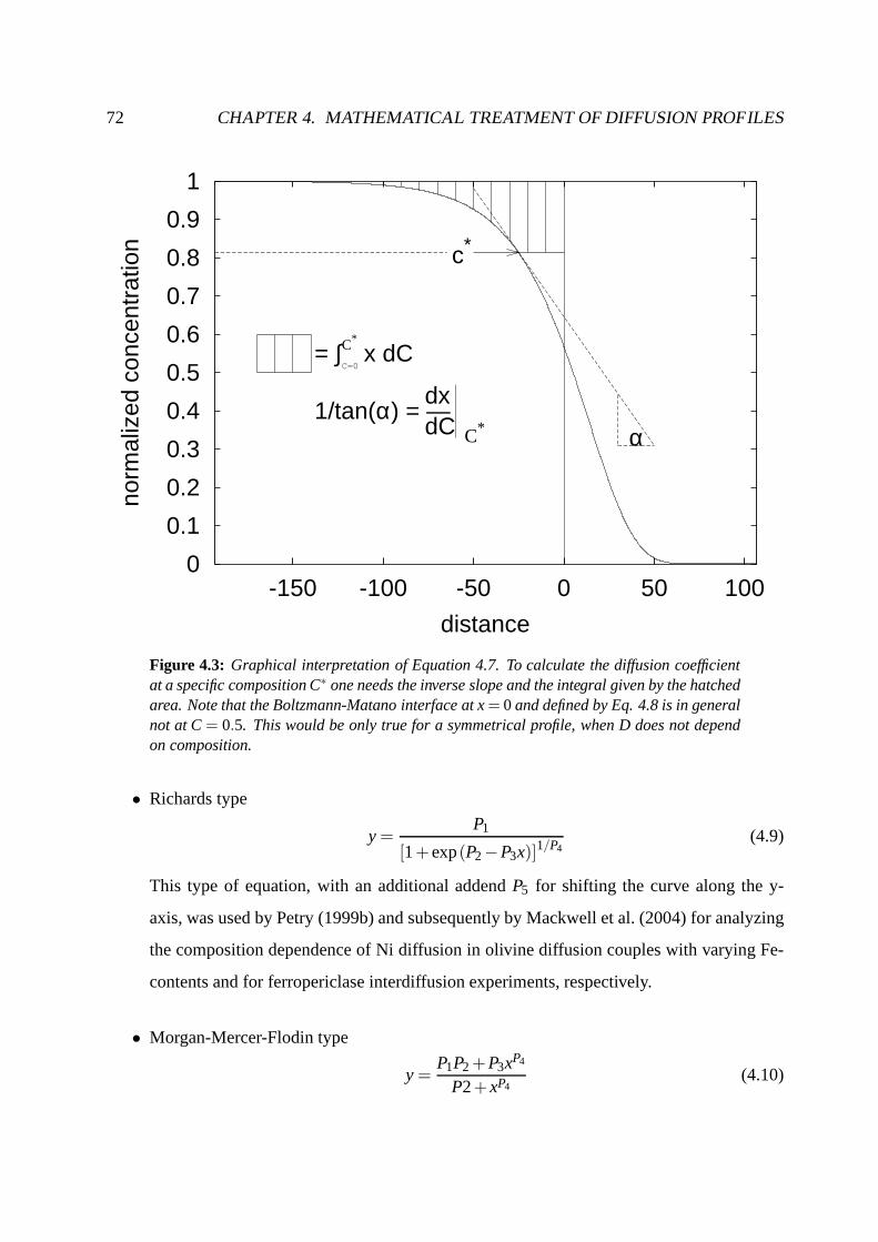
72 CHAPTER 4. MATHEMATICAL TREATMENT OF DIFFUSION PROFILES
0
0.1
0.2
0.3
0.4
0.5
0.6
0.7
0.8
0.9
1
-150 -100 -50 0 50 100
norm
aliz
ed c
once
ntra
tion
distance
α
= ∫C=0
C*
x dC
1/tan(α) = —dxdC C*
c*
Figure 4.3: Graphical interpretation of Equation 4.7. To calculate thediffusion coefficientat a specific composition C∗ one needs the inverse slope and the integral given by the hatchedarea. Note that the Boltzmann-Matano interface at x= 0 and defined by Eq. 4.8 is in generalnot at C= 0.5. This would be only true for a symmetrical profile, when D doesnot dependon composition.
• Richards type
y =P1
[1+exp(P2−P3x)]1/P4(4.9)
This type of equation, with an additional addendP5 for shifting the curve along the y-
axis, was used by Petry (1999b) and subsequently by Mackwellet al. (2004) for analyzing
the composition dependence of Ni diffusion in olivine diffusion couples with varying Fe-
contents and for ferropericlase interdiffusion experiments, respectively.
• Morgan-Mercer-Flodin type
y =P1P2+P3xP4
P2+xP4(4.10)
4.3. SEMI-INFINITE MEDIA, D CONCENTRATION-DEPENDENT 73
• Weibull type
y = P1−P2exp(
−P3xP4)
(4.11)
The fits of experimental data are not significantly differentemploying the different fit func-
tions given in Equations 4.9-4.11. Due to the strong nonlinearity of these functions, precise
fitting can be problematic as shown in Chapter 5. As an alternative, if fitting a single function
over the entire profile length is difficult, a combination of polynomials can be used.
4.3.2 Numerical simulations: Finite difference method
Numerical simulations of phenomena governed by partial differential equations are becoming
more and more important for many applications in science andtechnology such as continuum
mechanics, thermal conduction or diffusive mass transport. Different techniques for computation
exist, for example the finite element and the finite difference methods. For simulating diffusion
profiles numerically in this study a finite difference methodwas applied. The principle of the
technique is the discretization of the composition function C(x,t) in space and time and the ap-
proximation of the partial derivatives that arise in the diffusion equation, Eq. 1.2, by a Taylor
series expansion between the space and time nodes. Several monographs describing this method
in detail exist, e.g. Smith (1985) - a short introduction is also given in Crank (1979) and Ghez
(1988). To illustrate the technique, an example with an exponential composition dependence,
used for most of the composition-dependent problems in latter sections, is described here. An
example program for computation is given in Appendix C.
The diffusion equation, Equation 1.2, with D depending exponentially on composition, can
be written as:∂C∂t
=∂∂x
(
D0 ·exp(a ·C(x))∂C∂x
)
, (4.12)
which after differentiation gives:
∂C∂t
= a ·D0 ·exp(a ·C(x))
(
∂C∂x
)2
+D0 ·exp(a ·C(x)) · ∂2C∂x2 . (4.13)
Several finite difference schemes for solution may be employed. The simplest method for
approximation of the partial derivatives is the explicit formulation, also used in this study. An
74 CHAPTER 4. MATHEMATICAL TREATMENT OF DIFFUSION PROFILES
alternative would be for example an implicit finite difference scheme (Smith, 1985). The advan-
tage of this method is the unconditional stability but the drawback is that a large set of linear
equations has to be solved simultaneously. Therefore, the method is far more difficult to imple-
ment. Because no significant improvements of computationalspeed or accuracy are expected for
profiles investigated in this study, only the explicit method was implemented and is described
in the following paragraphs. The arguments for using the explicit instead of the more efficient
implicit method follow the same line of reasoning as in Gaetani and Watson (2002) in their study
of diffusive reequilibration of melt inclusions.
For implementation of an explicit finite difference scheme,the space coordinate of a diffu-
sion profile is divided into stepsδx and the time coordinate is divided into stepsδt (Fig. 4.4).
Expanding the concentration in time into a Taylor series gives:
C(i, j +1) = c(i, j)+δt∂C∂t
∣
∣
∣
∣
i, j+
12
(δt)2 ∂2C∂t2
∣
∣
∣
∣
i, j+ · · · (4.14)
If higher than linear terms are neglected the time derivative can be written as:
∂C∂t
∣
∣
∣
∣
i, j=
C(i, j + t)−c(i, j)δt
(4.15)
which according to Smith (1985) is first-order accurate inδt. The first derivative of the concen-
tration with respect to the space coordinate is expressed with a symmetric expression where the
Taylor series is used in the negative and positive x-direction:
∂C∂x
∣
∣
∣
∣
i, j=
C(i +1, j)−C(i −1, j)2δx
(4.16)
This expression has the advantage of being second-order accurate inδx and is therefore preferred
to simple backward or forward approximations (Ghez, 1988).A Taylor series expansion in the
x-direction truncated after the term containing the secondderivative of the concentration with
respect to distance leads to an expression of the second derivative of the compositionC with
respect tox:∂2C∂x2
∣
∣
∣
∣
i, j=
C(i +1, j)−2C(i, j)+C(i −1, j)
(δx)2 (4.17)
where the leading error is on the order ofδx2 (Smith, 1985).

4.3. SEMI-INFINITE MEDIA, D CONCENTRATION-DEPENDENT 75
u
u u uC(i,j+1)
C(i-1,j) C(i,j) C(i+1,j)
-�
6
?
δx δt
6 6
t
- x
Figure 4.4: Grid for performing the explicit finite difference method. Each node in space xi
and time ti represents a concentration C(xi , t j). The solution is propagated along the timeaxis by calculating the unknown concentration c(i,j+1) in terms of the known concentrationsC(i-1,j), C(i,j), and C(i+1,j) with the aid of Equation 4.18

76 CHAPTER 4. MATHEMATICAL TREATMENT OF DIFFUSION PROFILES
Inserting these finite difference approximations into the diffusion equation employing an
exponential composition dependence, Eq. 4.12, and rearranging finally results in:
C(i, j +1) = C(i, j)+ · · ·
+14
κ ·aD(i, j) [C(i +1, j)−C( j −1)]2+ · · ·
+κ ·D(i, j) [C(i +1, j)−2C(i, j)+C(i −1, j)] (4.18)
whereD(i, j) = D0exp(a ·C(i, j)) andκ = δt/(δx2). The conditionκ ·D(i, j) < 0.5 has to be
fulfilled, otherwise the algorithm becomes instable.
A numerical simulation is performed by applying Equation 4.18 repeatedly for each grid-
node of a new timestep until all timesteps add up to the duration of the experiment. As goodness
of fit criterion of a simulation, the sum of squared differences between the measured concentra-
tion Cm and the simulated concentrationCs at each distance-step∑δx
(Cm−Cs)2 is calculated and
minimized by iteratively changingD0 anda.
As a test of accuracy, Figure 4.5 compares simulations for different values ofκ ·D and an
analytical solution for composition-independentD (settinga in Eq. 4.12 equal to zero) using
a typical average value for ferropericlase diffusion experiments (Section 5.4) and 1200 sec of
diffusion. At values ofκ ·D ≥ 0.5 oscillations of calculated concentrations appear which rapidly
increase towards infinity for only slightly increasing values ofκ ·D, whereas for allκ ·D < 0.5
the overall deviation from the analytical solution is less than random scatter corresponding to
an analytical uncertainty of 0.1%. Hence, within the experimental error for the profile measure-
ments all simulations forκ ·D < 0.5 give accurate results in this example. This is in general true
for time scales up to 16 h, which is the longest timescale of experiments resulting in asymmetric
profiles investigated by finite difference simulations in this study.
As a second test of accuracy, Figure 4.6 and Table 4.1 comparediffusion coefficients derived
by the Boltzmann-Matano method, as a function of composition, performed on profiles first
derived by numerical simulations with varyingκ ·D values for a composition dependence of
D = 0.06·exp(3.4 ·C). The numerical simulations generate smooth input profiles without any
statistical scatter, hence to avoid inaccuracies due to an empirical fit-function, for Boltzmann-
Matano analysis an interpolation function supplied by the computer program Mathematica was
used as smoothing function.

4.3. SEMI-INFINITE MEDIA, D CONCENTRATION-DEPENDENT 77
0
0.1
0.2
0.3
0.4
0.5
100 110 120 130 140 150
norm
aliz
ed c
once
ntra
tion
distance, µm
analytical solutionκ D = 0.5021
κ D = 0.5κ D = 0.48
κ D = 0.1
Figure 4.5: Simulation for a diffusion profile with a constant diffusioncoefficient D of0.1 µ2 sec−1 and 1200 seconds of diffusion. Only one half of the profile is shown. Forvaluesκ ·D equal or slightly larger than 0.5 the simulations become instable whereas for allvalues less than 0.5 the solution agrees well with the analytical solution, Eq. 4.6, keeping inmind the statistical scatter in the profile analysis (see Chapter 3).
In this test, two completely independent methods are used tofirst generate the profile and
second to re-determine the composition-dependent diffusion coefficient. Thus, the consistency
between the results and the expected input diffusion coefficients given byD = 0.06·exp3.4 ·C,
on the order of 0.3 % (Table 4.1), indicates the accuracy of both methods. If one assumes
that the errors arising in the Boltzmann-Matano analysis are much smaller than the deviation of
the numerical simulations, because a smooth dataset was employed, than the deviations between
calculated diffusion coefficients and input diffusion coefficients solely originate by round-off and
discretization error in the numerical algorithm. The difference(Dreal−Dcalc)/Dreal in Table 4.1
is slightly larger for largerκ ·D and compositions in the steeper part of the asymmetric profile.
The overall variation of this deviation between 0.17 and 0.46 % is ∼ 2 orders of magnitude

78 CHAPTER 4. MATHEMATICAL TREATMENT OF DIFFUSION PROFILES
-13.4
-13.2
-13
-12.8
-12.6
-12.4
-12.2
-12
-11.8
-11.6
0 0.2 0.4 0.6 0.8 1
Log(
D, m
2 sec
-1)
composition, C
Log(0.06 · e3.4 · C)NoT = 4800, κ = 0.25
NoT = 12000, κ = 0.1
NoT = 1.2 · 106, κ = 0.001
Figure 4.6: Diffusion coefficients calculated by Boltzmann-Matano method using numericalsimulations with varying number of timesteps (NoT),κ values corresponding to 1200 sec ofdiffsuion and a composition-dependent diffusion coefficient: D = 0.06·exp(3.4·C).
smaller than the experimental error on D (∼ 30 %, see Chapter 5).
Therefore, the two different tests for a constant and a composition-dependent D confirm that
as long asκ ·D < 0.5 the numerical simulation is consistent with the diffusionequation, Eq. 4.12,
and accurate enough, within experimental error, for the experiments performed in this study.

4.3. SEMI-INFINITE MEDIA, D CONCENTRATION-DEPENDENT 79
Cnorm DS1, 1013 m2
sec DS2, 1013 m2
sec DS3, 1013 m2
sec Dreal, 1013 m2
secDreal−Dcalc
Dreal, %
NoT = 4800 NoT = 12000 NoT = 1200000 S1 S2 S3κ = 0.25 κ = 0.1 κ = 0.001
0.1 0.84 0.84 0.84 0.84 0.33 0.30 0.280.2 1.18 1.18 1.18 1.18 0.46 0.43 0.420.3 1.66 1.66 1.66 1.66 0.41 0.39 0.380.4 2.33 2.33 2.33 2.34 0.37 0.35 0.340.5 3.27 3.27 3.27 3.28 0.31 0.30 0.290.6 4.60 4.60 4.60 4.61 0.27 0.25 0.250.7 6.47 6.47 6.47 6.48 0.24 0.22 0.230.8 9.09 9.09 9.09 9.11 0.22 0.19 0.190.9 12.8 12.8 12.8 12.8 0.21 0.17 0.17
Table 4.1: Comparison of diffusion coefficients calculated by Boltzmann-Matano analy-sis using a finite difference simulation with a composition-dependent diffusion coefficientDreal = 0.06× exp(3.4 Cnorm), where Cnorm is a normalized composition between 0 and 1,as the input-profile. Three simulations were performed, models S1-S3, for a varying numberof timesteps (NoT) and correspondingκ values (δx= 1 µm), given in the topline of the table,to test if the resulting diffusion coefficients are consistent with each other.

80 CHAPTER 4. MATHEMATICAL TREATMENT OF DIFFUSION PROFILES
Chapter 5
Results
5.1 Introduction
In this chapter, the results of the diffusion experiments are described for olivine (Section 5.2),
wadsleyite (Section 5.3), ferropericlase (Section 5.4), and silicate perovskite (Section 5.5). The
observations include backscatter electron images of the diffusion couples and capsules, pro-
file examples measured by electron microprobe analysis (EPMA) and transmission electron mi-
croscopy equipped with an energy dispersive detector (EDX-TEM), and variation of diffusion
coefficients with pressure and temperature. Because most ofthe diffusion experiments have
been performed at different P-T conditions in capsules where the oxygen fugacity is buffered
by a solid state buffer system (either Ni-NiO or MgO-Fe, see Section 2.4), diffusion coefficients
are determined at variable oxygen fugacity conditions. Measurement of diffusion coefficients
D along a buffer system at different P and T conditions introduces variability from two sources
into the diffusion data: (I) Asf O2 changes along a buffer with temperature, the change inD
due to this variation inf O2 is absorbed into the temperature dependence, resulting in ahigher
activation energy determined in an Arrhenius plot comparedto the true activation energy at con-
stant temperature. (II) Thef O2-T relation itself shifts with a variation in pressure implying that
experiments carried out at the same temperature andf O2 buffer but at different pressures are not
equivalent. Ideally, corrections should be made for both ofthese effects in order to representD
as a function of the independent variables P, T andf O2.
In a review of garnet diffusion data (Chakraborty and Ganguly, 1991), obtained along the
graphite-O2 buffer, it is estimated that at pressures up to 4 GPa the effect of (II) is neglegible
81

82 CHAPTER 5. RESULTS
implying an insignificant difference either if the activation volume is determined using values
along the buffer or at constantf O2, whereas the effect of (I) yields an activation energy that is
∼ 10% larger than the value at constantf O2. In the studies of Farber et al. (2000) and Holzapfel
et al. (2003), where diffusion coefficients were determinedalong the Ni-NiO buffer, no attempt
was made to normalize the results to a constant oxyen fugacity. In this case, the values derived
for the activation energy and the activation volume are onlyvalid at conditions of the buffer
system used. The reason not to normalize the results to a constant value of f O2 in Holzapfel
et al. (2003) was the relatively large uncertainty in calculating the f O2 at high pressures. In
addition, the fact that the absolutef O2 of a solid buffer system changes with P and T implies
that the relativef O2 scale (f O2 relative to a buffer system) is a better indicator for the redox state
of the system than the absolutef O2 scale itself. Thef O2 inside the Earth most likely changes
subparallel tof O2 curves equivalent to solid state buffers (Frost, 1991). However, the activation
energy and activation volume are physical quantities strictly only defined at a constant oxygen
fugacity. Hence, in the present study, the effects of a changing f O2 of the Ni-NiO buffer as a
function of P and T (cases (I) and (II) defined above) is estimated using thermodynamic data of
the redox reaction in order to correct diffusion coefficients obtained using Ni-NiO capsules at
pressures below 24 GPa.
In Figure 5.1 the variation of the Ni-NiO buffer with pressure and temperature is shown
using values of Huebner (1971), Ride (1991), O’Neill and Pownceby (1993), and Pownceby and
O’Neill (1994). Ride (1991) lists an expression for the freeenergy change∆G0 of the oxidation
reaction of Ni:
Ni +12
O2 = NiO. (5.1)
The oxygen fugacity of reaction 5.1 can than be calculated at1 bar by
log( f O2) =2 ∆G0
R T ln(10). (5.2)
At elevated pressures, Equation 5.2 has to be rewritten as:
log( f O2) =2 (∆G0+
R P1 bar ∆V0(P,T)dP)
R T ln(10), (5.3)
where∆V0(P,T)dP is the volume change of Reaction 5.1. In model [1] in Figure 5.1 a constant
volume change of reaction 5.1 was assumed using molar volumes of Ni and NiO also given in
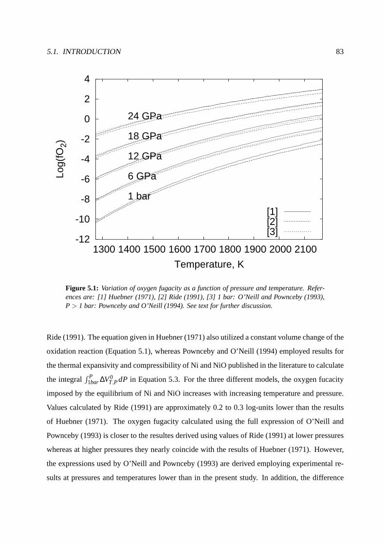
5.1. INTRODUCTION 83
-12
-10
-8
-6
-4
-2
0
2
4
1300 1400 1500 1600 1700 1800 1900 2000 2100
Log(
fO2)
Temperature, K
1 bar
6 GPa
12 GPa
18 GPa
24 GPa
[1][2][3]
Figure 5.1: Variation of oxygen fugacity as a function of pressure and temperature. Refer-ences are: [1] Huebner (1971), [2] Ride (1991), [3] 1 bar: O’Neill and Pownceby (1993),P > 1 bar: Pownceby and O’Neill (1994). See text for further discussion.
Ride (1991). The equation given in Huebner (1971) also utilized a constant volume change of the
oxidation reaction (Equation 5.1), whereas Pownceby and O’Neill (1994) employed results for
the thermal expansivity and compressibility of Ni and NiO published in the literature to calculate
the integralR P
1bar ∆V0T,PdP in Equation 5.3. For the three different models, the oxygen fucacity
imposed by the equilibrium of Ni and NiO increases with increasing temperature and pressure.
Values calculated by Ride (1991) are approximately 0.2 to 0.3 log-units lower than the results
of Huebner (1971). The oxygen fugacity calculated using thefull expression of O’Neill and
Pownceby (1993) is closer to the resultes derived using values of Ride (1991) at lower pressures
whereas at higher pressures they nearly coincide with the results of Huebner (1971). However,
the expressions used by O’Neill and Pownceby (1993) are derived employing experimental re-
sults at pressures and temperatures lower than in the present study. In addition, the difference
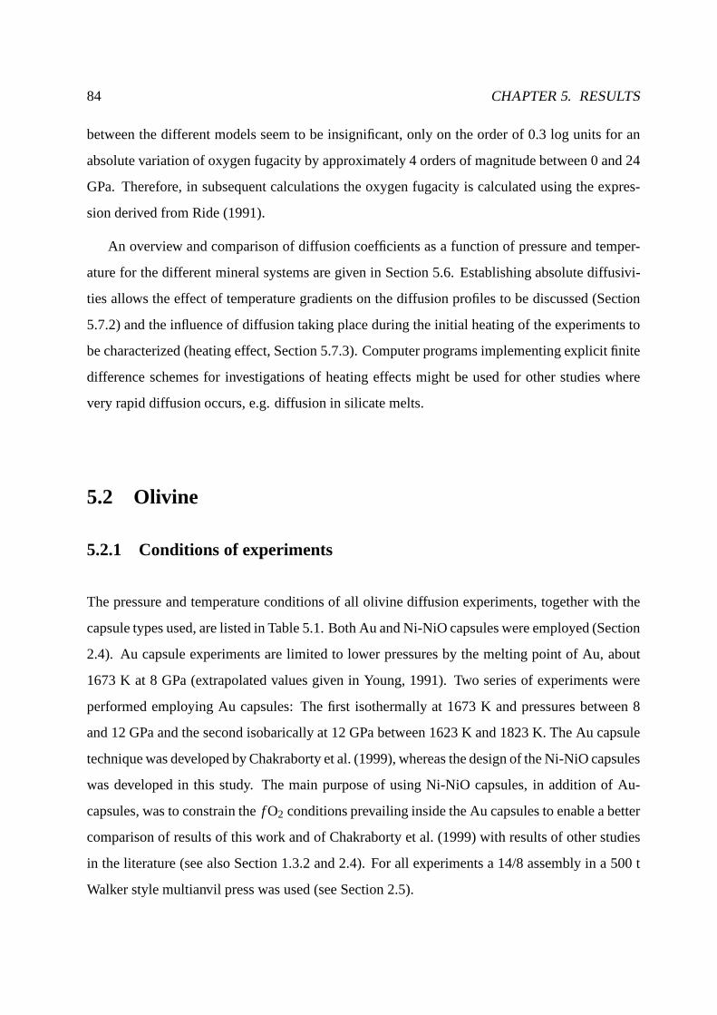
84 CHAPTER 5. RESULTS
between the different models seem to be insignificant, only on the order of 0.3 log units for an
absolute variation of oxygen fugacity by approximately 4 orders of magnitude between 0 and 24
GPa. Therefore, in subsequent calculations the oxygen fugacity is calculated using the expres-
sion derived from Ride (1991).
An overview and comparison of diffusion coefficients as a function of pressure and temper-
ature for the different mineral systems are given in Section5.6. Establishing absolute diffusivi-
ties allows the effect of temperature gradients on the diffusion profiles to be discussed (Section
5.7.2) and the influence of diffusion taking place during theinitial heating of the experiments to
be characterized (heating effect, Section 5.7.3). Computer programs implementing explicit finite
difference schemes for investigations of heating effects might be used for other studies where
very rapid diffusion occurs, e.g. diffusion in silicate melts.
5.2 Olivine
5.2.1 Conditions of experiments
The pressure and temperature conditions of all olivine diffusion experiments, together with the
capsule types used, are listed in Table 5.1. Both Au and Ni-NiO capsules were employed (Section
2.4). Au capsule experiments are limited to lower pressuresby the melting point of Au, about
1673 K at 8 GPa (extrapolated values given in Young, 1991). Two series of experiments were
performed employing Au capsules: The first isothermally at 1673 K and pressures between 8
and 12 GPa and the second isobarically at 12 GPa between 1623 Kand 1823 K. The Au capsule
technique was developed by Chakraborty et al. (1999), whereas the design of the Ni-NiO capsules
was developed in this study. The main purpose of using Ni-NiOcapsules, in addition of Au-
capsules, was to constrain thef O2 conditions prevailing inside the Au capsules to enable a better
comparison of results of this work and of Chakraborty et al. (1999) with results of other studies
in the literature (see also Section 1.3.2 and 2.4). For all experiments a 14/8 assembly in a 500 t
Walker style multianvil press was used (see Section 2.5).

5.2. OLIVINE 85
Sample Capsule T, K P, GPa t, min log(DFe−Mg/m2
sec) log(DNi/m2
sec) log(DMn/m2
sec)1CS12 Au 1673 12 1440 -16.2(3) -16.5(4) -16.1(5)2CS10 Au 1673 10 1440 -16.4(3) -15.5(4) -16.4(5)3CS8 Au 1673 8 1440 -15.6(3) -15.7(4) -15.8(5)4CS11 Au 1673 11 1440 -15.5(3) -15.7(4) -15.4(5)5CS12 Au 1673 12 1440 -16.3(3) -16.4(4) -16.1(5)6CS10 Au 1673 10 1440 -16.3(3) -15.5(4) -16.5(5)7CS11.5 Au 1673 11.5 1440 -16.1(3) -15.8(4) -16.2(5)8CS10.5 Au 1673 10.5 1440 -16.1(3) -15.5(4) -15.9(5)9CS11 Au 1673 11 1440 -15.3(3) -15.4(4) -15.5(5)10CS11.5 Au 1673 11.5 1440 -16.3(3) -16.1(4) -16.3(5)13CS12 Au 1773 12 1440 -15.9(3) -16.1(4) -16.0(5)14CS12 Au 1723 12 1440 -16.1(3) -16.3(4) -16.2(5)15CS12 Au 1823 12 1440 -15.5(3) -15.6(4) -15.6(5)16CS12 Au 1623 12 4320 -16.8(3) -16.9(4) -16.5(5)17CS12 Ni-NiO 1673 12 1443 -16.7(3) -16.6(4) -16.7(5)18CS6 Ni-NiO 1673 6 1440 -15.7(3) n.m. n.m.20CS6 Ni-NiO 1673 6 1440 -15.4(3) -15.4(3) -15.5(5)
Table 5.1: Results and conditions of the olivine high pressure diffusion runs - Diffusioncoefficients are given inlog10(D), n.m. denotes not measured (see text for explanation,Section 5.2.3)
5.2.2 Characterization of diffusion couples after the experiments
To detect and exclude irregular artifacts along the diffusion interface due to possible instabilities
of the diffusion front, all samples have been studied by highresolution backscattered electron
imaging (Figure 5.2) and elemental mapping. Diffusion fronts are usually regular and paral-
lel to the crystal interface. In one experiment, 20CS6, the central part of the diffusion couple
sheared between two cracks (formed probably during initialcompression) and recrystallized.
Grain boundary diffusion is evident in backscatter electron images and elemental maps. For
measuring diffusion profiles, undisturbed areas outside the shear zone were investigated, where
the original single crystal structure remained intact.
Sometimes, the two crystals of the diffusion couple separated at the interface due to decom-
pression and/or sample preparation. The length scale of this separation is much less then 1µm
and therefore insignificant with respect to profile shape andlength (normally≥ 10 µm, see be-
low).
The thermocouple and the capsule in the 14/8 assemblies (Section 2.5) used for the olivine

86 CHAPTER 5. RESULTS
Olivinediffusion couple
Au capsuleMgO
TCAl2O3
LaCrO3 furnace
A
olivinedifffusioncouple
NiO
Ni cpsule
TC
MgO
LaCrO3 furnace
B
Figure 5.2: Backscattered electron images of the two capsule types used: A gold capsule, BNi-NiO capsule (see Section 2.4). For all experiments a 14/8assembly was employed. Thestep of the inner LaCrO3 furnace-part is visible in A and B.
experiments were effectively shielded from each other by a MgO disc (Fig. 2.6 and 5.2) and no
Ni contamination could be detected in the thermocouple. With Ni-NiO capsules, prevention of

5.2. OLIVINE 87
this effect is utterly important because otherwise Ni can diffuse into the thermocouple, seriously
influencing the temperature reading. In initial experiments, employing Au capsules, instead of
using a lid covering the capsule and the MgO cylinder separating the capsule from the furnace, a
MgO plug was used on top of the capsule. In this case, the Au extruded from the capsule between
the plug and the inner wall of the MgO cylinder into the bore holes of the Al2O3 thermocouple
sleeve. Because the Au did not react with the thermocouple, the temperature reading was not
significantly effected.
Water potentially influences diffusion rates in olivine as shown in the study of Mei and
Kohlstedt (2000) for diffusional creep, which depends on Sidiffusion. To characterize the water
contents of the crystals, infrared spectra were measured onsample 8CS10.5 employing a Bruker
IFS 120 HR high resolution FTIR spectrometer. The syntheticforsterite contained no detectable
amounts of water whereas the San Carlos olivine had on the order of 25 ppm by weight water
based on the absorption correction of Paterson (1982) afterthe experiment.

88 CHAPTER 5. RESULTS
5.2.3 Profiles and diffusion coefficients
Example profiles for Fe, Mg, Ni, and Mn are shown in Figure 5.3.The profiles analyzed by
EPMA are symmetrical for the experiments described here, whereas strongly asymmetric pro-
files were observed by Chakraborty (1997). This apparent discrepancy can be explained by the
limited compositional range, Fo100-Fo94, used in this study (Section 2.3.2). Hence, the composi-
tion dependence of diffusion cannot be resolved in the experiments reported here using profiles
determined by EPMA (for analysis employing EDX-STEM see below), and the diffusion coeffi-
cient is representative of the average composition of the diffusion couple (Mg# = 0.97). This is
the case for the Fe-Mg interdiffusion coefficient and also for Mn and Ni diffusion. The length of
the diffusion profiles is approximately 10-20µm and therefore much smaller than the length of
the single crystals forming the diffusion couple. Thus, theprofiles were analyzed with Equation
4.6, the analytical solution of the diffusion equation (Equation 1.2) using initial and boundary
conditions given by Equations 4.2 and 4.3. For fitting the profiles to Equation 4.6 the nonlinear
least square fit routine supplied by the computer program Mathematica (Version 4.2.0.0) was em-
ployed for solving for 2√
Dt and the position of the interfacea, with respect to the lab reference
frame (xlab, for a discussion of different reference frames see Brady, 1975b):
C(x, t) =12·erfc
xlab−a
2√
Dt. (5.4)
The fitted function was always checked by eye and starting values or number of iterations were
systematically changed if necessary.
Diffusion coefficients derived by the procedure just outlined are listed in Table 5.1. The error
was estimated first by the scatter associated with differentprofile measurements on the same sam-
ple and with profiles measured on samples at the same conditions (experimental reproducibility).
This error is on the order of 0.2 log-units for Fe-Mg interdiffusion, corresponding to a relative
error of 50%. For Ni and Mn, errors of 0.3 and 0.4 log-units, respectively, were estimated. The
increased error of Ni and Mn diffusion coefficients comparedto Fe-Mg interdiffusion coeffi-
cients is caused by the larger analytical scatter for the twotrace elements (see Fig. 5.3). As
shown later in Sections 5.2.4, 5.2.5 and in the ferropericlase system (Section 5.4) the error for
high pressure multianvil diffusion experiments is somewhat larger because of errors in pressure
and temperature. Hence, the overall error for the high pressure experiments in the olivine system

5.2. OLIVINE 89
1.86
1.88
1.9
1.92
1.94
1.96
1.98
2
0 5 10 15 20 25 30 35 40
0
0.02
0.04
0.06
0.08
0.1
0.12
0.14
Mg
on th
e ba
sis
of 4
oxy
gen
Fe
on th
e ba
sis
of 4
oxy
gen
distance µmA
MgFe
0
0.0005
0.001
0.0015
0.002
0.0025
0.003
0.0035
0.004
0 5 10 15 20 25 30 35 40
Mn
on th
e ba
sis
of 4
O
distance, µm
B
Mn
0
0.001
0.002
0.003
0.004
0.005
0.006
0 5 10 15 20 25 30 35 40
Ni o
n th
e ba
sis
of 4
O
distance, µm
C
Ni
Figure 5.3: Diffusion profile examples for olivine measured by EPMA (electron microprobe).The experiment was performed at 12 GPa, 1623 K and annealed for 72 h (16CS12). In (A)the Fe and the Mg profiles are shown together. The Fe-Mg interdiffusion coefficient can bederived from either of the two profiles (Section 1.2.3). In (B) the Mn profile and in (C) the Niprofile are shown.

90 CHAPTER 5. RESULTS
XcDtDc
% error7 0.96 46 0.95 55 0.93 84 0.89 123 0.80 242 0.56 79
Table 5.2: Error of the true diffusion coefficient Dt given in % deviation of Dt from thediffusion coefficient Dc determined from a convolved profile. The ratio Dt/Dc was calculatedemploying Equation (20) given in Ganguly et al. (1988, see also Eq. 5.5). Xc denotes half-length of the profile in microns.
is on the order of 0.3 log-units for Fe-Mg interdiffusion, 0.4 log-units for Ni and 0.5 log-units
for Mn diffusion.
Because some of the profiles are only∼ 8−10 µm long, they may be susceptible to convo-
lution effects. The possible effect of profile broadening, due to the finite excitation volume of the
X-rays (Section 3.2), was estimated using the algorithm developed by Ganguly et al. (1988). The
standard deviationε of the X-ray excitation volume, assuming a Gaussian intensity distribution,
was determined to be better than 0.46µm. This value was derived by scanning across the Al2O3-
MgO boundary between the thermocouple sleeve and the MgO cylinder (compare with Figure
2.7) in the low-temperature part of the assembly. The effectof convolution can be estimated
employing Equation (20) of Ganguly et al. (1988):
Dt
Dc= 1−8
(
εXc
)2
(5.5)
whereDt is the true diffusion coefficient,Dc denotes the apparent diffusion coefficient deter-
mined from the profile subject to convolution broadening andXc is the half width of the profile.
This equation is only valid for a composition-independent diffusion coefficient. Table 5.2 shows
errors as percent deviation from the true diffusion coefficientDt for profile half widths between 2
and 7µm. If an error of 12% is considered as acceptable, keeping theexperimental uncertainties
in mind (see above), profiles as short as 8µm still give reliable diffusion coefficients.
To verify these calculations, two samples, 6CS10 and 17CS12(Table 5.1), with diffusion
profile lengths of 10 and 8µm, respectively, were analyzed by EDX-STEM following the ex-
perimental procedure developed by Meißner et al. (1998) anddescribed in Section 3.3. Figure

5.2. OLIVINE 91
5.4 shows the profiles for both samples. In both cases the difference for diffusion coefficients
determined by fitting a composition-independent diffusioncoefficient is on the order of 30%,
somewhat larger than estimated in Table 5.2. As outlined above the difference in D for different
profiles determined on the same sample is as large as 0.2 log-units corresponding to a relative
error of∼ 50%. Therefore, profiles measured by EPMA, show no significant convolution effects
with respect to the average diffusion coefficient of the profile.
However, Figure 5.4 shows also that the composition-dependence of diffusion can be resolved
by EDX-STEM, whereas the subtle asymmetry of the profiles is not detectable by EPMA. For
both samples shown in Figure 5.4, 6CS10 and 17CS12, an assymetric fit employing a composi-
tion factor of exp(6.9 XFe2SiO4), observed at 1 bar (Chakraborty, 1997, Dohmen, pers. com.),is
fully compatible with the TEM profiles. Hence, to correct Fe-Mg interdiffusion coefficients at
XFe2SiO4 = 0.97, as determined in this study, toXFe2SiO4 = 0.90, the average olivine composition
in the upper mantle, requires the addition of 0.2-0.3 log-units.
Sample 18CS6 at 6 GPa and 1673 K (Table 5.1) employed a slightly different Ni-NiO cap-
sule than originally developed in this study (Section 2.4).Instead of using Ni-foil, a Ni-wire
was drilled similar to the Au capsule design. After the diffusion experiment the olivine diffusion
couple showed Mn contamination along the rim of the crystalsand across the diffusion zone.
Hence, a peak-shaped Mn distribution developed across the interface (up to 3.7 wt% MnO). This
phenomenon can only be explained by Mn or MnO contamination from the capsule. Because
the capsule was produced from high-purity Ni-wire, the Mn contamination of the capsule pre-
sumably occurred during drilling (e.g. by a Mn-bearing drill bit). Therefore, only the Fe-profile
was analyzed in this sample, because 3.7 wt% MnO does not alter the thermodynamic factor for
Fe-Mg interdiffusion significantly, implying no change of the Fe-Mg interdiffusion coefficient as
compared to the Mn-free system. This is not clear for Ni diffusion. Therefore, Ni profiles were
omitted for sample 18CS6 when deriving diffusion coefficients.

92 CHAPTER 5. RESULTS
0
0.2
0.4
0.6
0.8
1
20 25 30 35 40
norm
aliz
ed c
once
ntra
tion
distance, µm
A, 6CS10
EPMAEPMA, Dconst
EDX-TEMEDX-TEM, Dconst
EDX-TEM, Dco-dep
0
0.2
0.4
0.6
0.8
1
0 2 4 6 8 10 12 14
norm
aliz
ed c
once
ntra
tion
distance, µm
B, 17CS12
EPMAEPMA, Dconst
EDX-TEMEDX-TEM, Dco-dep
Figure 5.4: Comparison of Fe-profiles (normalized concentration) measured by EPMA andEDX-TEM for samples 6CS10 (A) and 17CS12 (B, see Table 5.1). For fitting the data ananalytical solution (Eq. 5.4) was used (Dconst) or a simulation employing an exponentialcomposition dependence (Dco−dep), as discussed in the text.
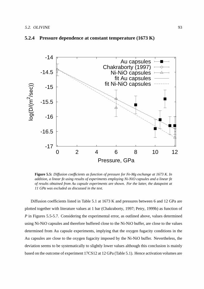
5.2. OLIVINE 93
5.2.4 Pressure dependence at constant temperature (1673 K)
-17
-16.5
-16
-15.5
-15
-14.5
-14
0 2 4 6 8 10 12
log(
D/(
m2 /s
ec))
Pressure, GPa
Au capsulesChakraborty (1997)
Ni-NiO capsulesfit Au capsules
fit Ni-NiO capsules
Figure 5.5: Diffusion coefficients as function of pressure for Fe-Mg exchange at 1673 K. Inaddition, a linear fit using results of experiments employing Ni-NiO capsules and a linear fitof results obtained from Au capsule experiments are shown. For the latter, the datapoint at11 GPa was excluded as discussed in the text.
Diffusion coefficients listed in Table 5.1 at 1673 K and pressures between 6 and 12 GPa are
plotted together with literature values at 1 bar (Chakraborty, 1997; Petry, 1999b) as function of
P in Figures 5.5-5.7. Considering the experimental error, asoutlined above, values determined
using Ni-NiO capsules and therefore buffered close to the Ni-NiO buffer, are close to the values
determined from Au capsule experiments, implying that the oxygen fugacity conditions in the
Au capsules are close to the oxygen fugacity imposed by the Ni-NiO buffer. Nevertheless, the
deviation seems to be systematically to slightly lower values although this conclusion is mainly
based on the outcome of experiment 17CS12 at 12 GPa (Table 5.1). Hence activation volumes are

94 CHAPTER 5. RESULTS
-17
-16.5
-16
-15.5
-15
-14.5
-14
-13.5
0 2 4 6 8 10 12
log(
D/(
m2 /s
ec))
pressure, GPa
Au capsulesNi-NiO capsules
Petry (1999)fit Au capsules
fit Ni-NiO capsules
Figure 5.6: Diffusion coefficients as function of pressure for Ni at 1673K. In addition, alinear fit using results of experiments employing Ni-NiO capsules and a linear fit of resultsobtained from Au capsule experiments are shown. For the latter, the datapoint at 11 GPawas excluded as discussed in the text.
calculated for both the complete dataset and for the experiments performed in Ni-NiO capsules
alone to be able to judge if a statistically-significant difference exists.
For comparison, diffusion data for Fe-Mg exchange at 1 bar are taken from Chakraborty
(1997), where an Arrhenius plot is given for Fo86 and Fo92 compositions at an oxygen fugacity
of 10−12 bar (Fig. 5 in Chakraborty, 1997). The logarithm of the Fe-Mginterdiffusion co-
efficient at 1673 K andXFe2SiO4 = 0.08 is log(DFe−Mg) = −15.36. Taking the compositional
dependence, as discussed in the previous section (Section 5.2.3), into account, the correspond-
ing value for Fo97 is approximately 0.3 log-units smaller. The fO2 effect is corrected with an
oxygen fugacity exponent of 1/5, consistent with recent experimental results of Dohmen (pers.
communication). Hence, the logarithm of the Fe-Mg interdiffusion coefficient at 1 bar, 1673
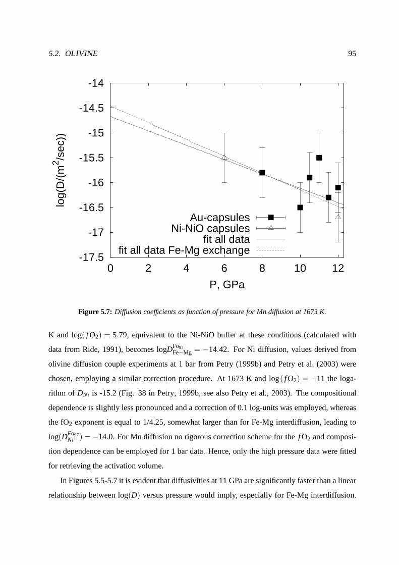
5.2. OLIVINE 95
-17.5
-17
-16.5
-16
-15.5
-15
-14.5
-14
0 2 4 6 8 10 12
log(
D/(
m2 /s
ec))
P, GPa
Au-capsulesNi-NiO capsules
fit all datafit all data Fe-Mg exchange
Figure 5.7: Diffusion coefficients as function of pressure for Mn diffusion at 1673 K.
K and log( f O2) = 5.79, equivalent to the Ni-NiO buffer at these conditions (calculated with
data from Ride, 1991), becomes logDFo97Fe−Mg = −14.42. For Ni diffusion, values derived from
olivine diffusion couple experiments at 1 bar from Petry (1999b) and Petry et al. (2003) were
chosen, employing a similar correction procedure. At 1673 Kand log( f O2) = −11 the loga-
rithm of DNi is -15.2 (Fig. 38 in Petry, 1999b, see also Petry et al., 2003). The compositional
dependence is slightly less pronounced and a correction of 0.1 log-units was employed, whereas
the fO2 exponent is equal to 1/4.25, somewhat larger than for Fe-Mg interdiffusion, leading to
log(DFo97Ni ) = −14.0. For Mn diffusion no rigorous correction scheme for thef O2 and composi-
tion dependence can be employed for 1 bar data. Hence, only the high pressure data were fitted
for retrieving the activation volume.
In Figures 5.5-5.7 it is evident that diffusivities at 11 GPaare significantly faster than a linear
relationship between log(D) versus pressure would imply, especially for Fe-Mg interdiffusion.
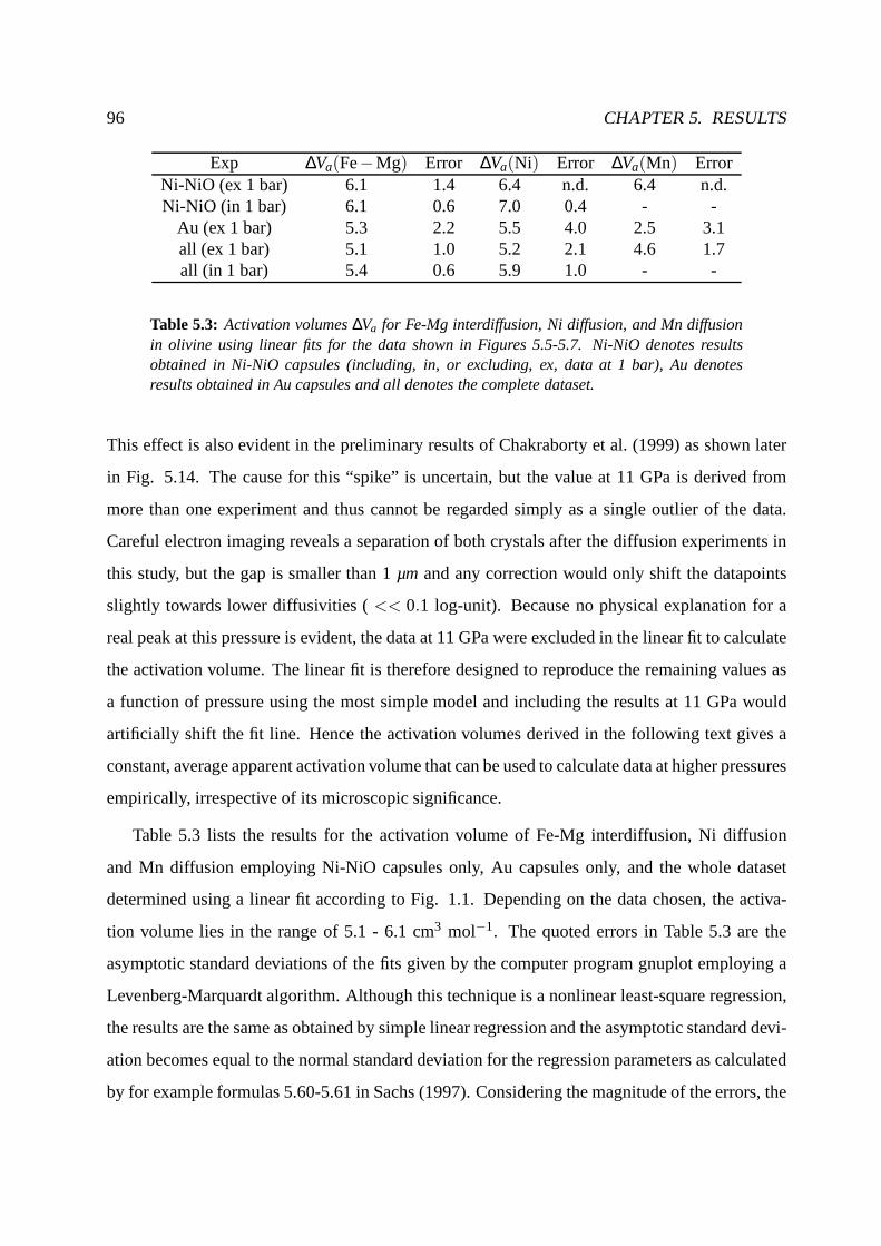
96 CHAPTER 5. RESULTS
Exp ∆Va(Fe−Mg) Error ∆Va(Ni) Error ∆Va(Mn) ErrorNi-NiO (ex 1 bar) 6.1 1.4 6.4 n.d. 6.4 n.d.Ni-NiO (in 1 bar) 6.1 0.6 7.0 0.4 - -
Au (ex 1 bar) 5.3 2.2 5.5 4.0 2.5 3.1all (ex 1 bar) 5.1 1.0 5.2 2.1 4.6 1.7all (in 1 bar) 5.4 0.6 5.9 1.0 - -
Table 5.3: Activation volumes∆Va for Fe-Mg interdiffusion, Ni diffusion, and Mn diffusionin olivine using linear fits for the data shown in Figures 5.5-5.7. Ni-NiO denotes resultsobtained in Ni-NiO capsules (including, in, or excluding, ex, data at 1 bar), Au denotesresults obtained in Au capsules and all denotes the completedataset.
This effect is also evident in the preliminary results of Chakraborty et al. (1999) as shown later
in Fig. 5.14. The cause for this “spike” is uncertain, but thevalue at 11 GPa is derived from
more than one experiment and thus cannot be regarded simply as a single outlier of the data.
Careful electron imaging reveals a separation of both crystals after the diffusion experiments in
this study, but the gap is smaller than 1µmand any correction would only shift the datapoints
slightly towards lower diffusivities (<< 0.1 log-unit). Because no physical explanation for a
real peak at this pressure is evident, the data at 11 GPa were excluded in the linear fit to calculate
the activation volume. The linear fit is therefore designed to reproduce the remaining values as
a function of pressure using the most simple model and including the results at 11 GPa would
artificially shift the fit line. Hence the activation volumesderived in the following text gives a
constant, average apparent activation volume that can be used to calculate data at higher pressures
empirically, irrespective of its microscopic significance.
Table 5.3 lists the results for the activation volume of Fe-Mg interdiffusion, Ni diffusion
and Mn diffusion employing Ni-NiO capsules only, Au capsules only, and the whole dataset
determined using a linear fit according to Fig. 1.1. Depending on the data chosen, the activa-
tion volume lies in the range of 5.1 - 6.1 cm3 mol−1. The quoted errors in Table 5.3 are the
asymptotic standard deviations of the fits given by the computer program gnuplot employing a
Levenberg-Marquardt algorithm. Although this technique is a nonlinear least-square regression,
the results are the same as obtained by simple linear regression and the asymptotic standard devi-
ation becomes equal to the normal standard deviation for theregression parameters as calculated
by for example formulas 5.60-5.61 in Sachs (1997). Considering the magnitude of the errors, the

5.2. OLIVINE 97
difference between the activation volumes derived in Table5.3 is not statistically significant. In
addition, the difference in absolute diffusivities and theextrapolation towards a pressure of 1 bar
implies that the values derived from Au capsule experimentsare representative for diffusivities
at an oxygen fugacity close or slightly higher than the Ni-NiO buffer.
For Ni-diffusion the data for the activation volumes are in the range of 5.5±1.0 cm3 mol−1
to 7.0±0.4 cm3 mol−1, for a fit of results employing Au capsules and a fit for Ni-NiO buffered
data (including the 1 bar value of Petry et al., 2003), respectively. The uncertainty of the results
obtained for Ni diffusion is much larger than for Fe-Mg interdiffusion. Hence, the activation
volumes determined for Fe-Mg interdiffusion and for Ni diffusion are very close to each other
within error (Table 5.3). The same statistical arguments asused for Fe-Mg exchange with respect
to the f O2 conditions prevailing inside the Au capsules experiments apply for Ni diffusion as
well. Thus, diffusivities determined using Ni-NiO capsules and Au capsules are very close to
each other.
For Mn diffusion, the activation volume using results of experiments performed in Au cap-
sules is 2.5±3.1 cm3 mol−1. The large analytical scatter of the Mn results, is the reason for the
large uncertainty. Only a fit using all data results in a statistically significant activation volume of
4.6±1.7 cm3 mol−1, fully compatible with values derived for Fe-Mg interdiffusion (Table 5.3).
Therefore, in Figure 5.7, the fit for Fe-Mg interdiffusion isshown in addition to the fit for the
Mn diffusion coefficients. Within the scatter of the data, the regression of Fe-Mg interdiffusion
coefficients if fully compatible with the results for Mn. Theextrapolated diffusivity at 1 bar is
log(DMn) =−14.7, which is close to the value of Fe-Mg interdiffusion (log(
DFe−Mg)
=−14.4).
Based on the results presented in this section it can be concluded that the diffusion coefficients
determined for divalent cations in olivine are close to eachother, as already observed in studies at
1 bar (e.g. Petry et al., 2003). This is also true for the activation volume of diffusion which, for all
three diffusion processes, lies in the range 4.0−7.0 cm3 mol−1. Because no statistical significant
difference between diffusion coefficients determined fromexperiments employing Au capsules
and from those employing Ni-NiO capsules was found, the activation volume derived by a fit of
all diffusion data in one system is regarded as the best estimate of the true activation volume at
1673 K and anf O2 close to the corresponding value of the Ni-NiO buffer. Hencethe most likely

98 CHAPTER 5. RESULTS
value for Fe-Mg interdiffusion is 5.6±1.0 cm3 mol−1. This would be the recommended value
to use for the other elements as well, although consideration of formal errors suggests 4-7 cm3
mol−1 based on data from various trace elements. This best fit valueis also essentially the same
as found for Fe-Mg interdiffusion by Misener (1974).
As discussed above, the values for the activation volume of Fe-Mg interdiffusion, Ni diffusion
and Mn diffusion so far derived are valid along the Ni-NiO buffer. Therefore, the values ofVa
include the variation off O2 representative of the Ni-NiO buffer. Strictly, the activation volume is
defined for a constant oxygen fugacity. This is only possibleif the oxygen fugancity variation of
the Ni-NiO buffer can be calculated as a function of pressureand temperature. Literature values
published so far can only be used as an approximation becauseof difficulties of measuring the
oxygen potential at high pressures. Using values given in Ride (1991), the variation off O2 at
1673 K is between logf O2 = −5.8 at 1 bar to logf O2 = −2.5 at 12 GPa, assuming a constant
volume of the oxidation reaction of Ni (see Section 5.1 for further explanations). This change
in f O2 corresponds to a change of 0.7 log units of diffusivity. Therefore an activation volume
of 5.6 cm3 mol−1 along the Ni-NiO buffer corresponds to a value of 7.4 cm3 mol−1 at constant
oxygen fugacity.
5.2.5 Temperature dependence at constant pressure (12 GPa)
To constrain the temperature dependence at elevated pressures, experiments at variable temper-
atures between 1623 K and 1823 K have been performed employing Au capsules. Diffusion
coefficients for Fe-Mg interdiffusion, Ni diffusion and Mn diffusion are given in Table 5.1 and
are displayed in Arrhenius plots in Figures 5.8-5.10. In allcases a linear trend without any sig-
nificant kink is observed indicating that the diffusion mechanism does not change for divalent
cations at 12 GPa in the temperature range 1623-1823 K. The slope over this temperature range
is interpreted to be representative for the transition metal-extrinsic (TaMED) regime (Section
1.2.3). Hence, the activation energy is close to, but not exactly, the migration energy.
The activation energy at high pressure,EPa , calculated from the slope of the regression lines
in Figures 5.8-5.10 is related to the activation energy at 1 bar,E1a, by:
(
∂lnD
∂ 1T
)
P
= −EPa
R= −E1
a +P ·∆Va
R(5.6)

5.2. OLIVINE 99
-17.2-17
-16.8-16.6-16.4-16.2
-16-15.8-15.6-15.4-15.2
-15
5.5 5.6 5.7 5.8 5.9 6 6.1 6.2
16231673172317731823
log(
D)
10000/T, 1/K
T, K
Figure 5.8: Diffusion coefficients as a function of inverse temperaturefor Fe-Mg exchangeat 12 GPa using Au capsules.
as shown in Section 1.2.6 and Figure 1.1, assuming that the preexponential factor is pressure
independent. In addition, as shown in the last section, the diffusion coefficients obtained using
Au capsules follow a trend compatible with a change inf O2 consistent with the Ni-NiO buffer,
rather than representing values at constantf O2. Therefore the slope determined from a plot of
logD versus inverse temperature must also consist of af O2 contribution. Formally this con-
tribution can be derived by considering the total differential of log(D) with respect to inverse
temperature andf O2 at constant pressure:
(dlnD)P =
(
∂lnD
∂ 1T
)
f O2,P
(
∂1T
)
P+
(
∂lnD∂ln f O2
)
P, 1T
(∂ln f O2)P . (5.7)

100 CHAPTER 5. RESULTS
-17.5
-17
-16.5
-16
-15.5
-15
5.5 5.6 5.7 5.8 5.9 6 6.1 6.2
13501400145015001550
log(
D)
10000/T, 1/K
T, K
Figure 5.9: Diffusion coefficients as a function of inverse temperaturefor Ni at 12 GPa usingAu capsules.
Equation 5.7 can be rewritten as:
(dlnD)P = −Ea
R
(
∂1T
)
P+
(
∂lnD∂ln f O2
)
P, 1T
(
∂ln f O2
∂ 1T
)
NNO,P
(
∂1T
)
P. (5.8)
Hence, the activation energy at high pressure including theeffect of f O2, E∗a, is:
E∗a = EP,c
a −R
(
∂lnD∂ln f O2
)
P, 1T
(
∂ln f O2
∂ 1T
)
NNO,P
, (5.9)
whereHP,ca is the activation energy at high pressure and constantf O2. From recent experimental
results, the dependence of the Fe-Mg interdiffusion coefficient on oxygen fugacity can be de-
scribed with an exponent of 1/4.5 - 1/5.5 (Petry et al., 2003). Hence, an average value of 1/5
is assumed in this study. The temperature dependence of oxygen fugacity corresponding to the
Ni-NiO buffer (NNO) at 12 GPa is much less well constrained. If a constant volume change,
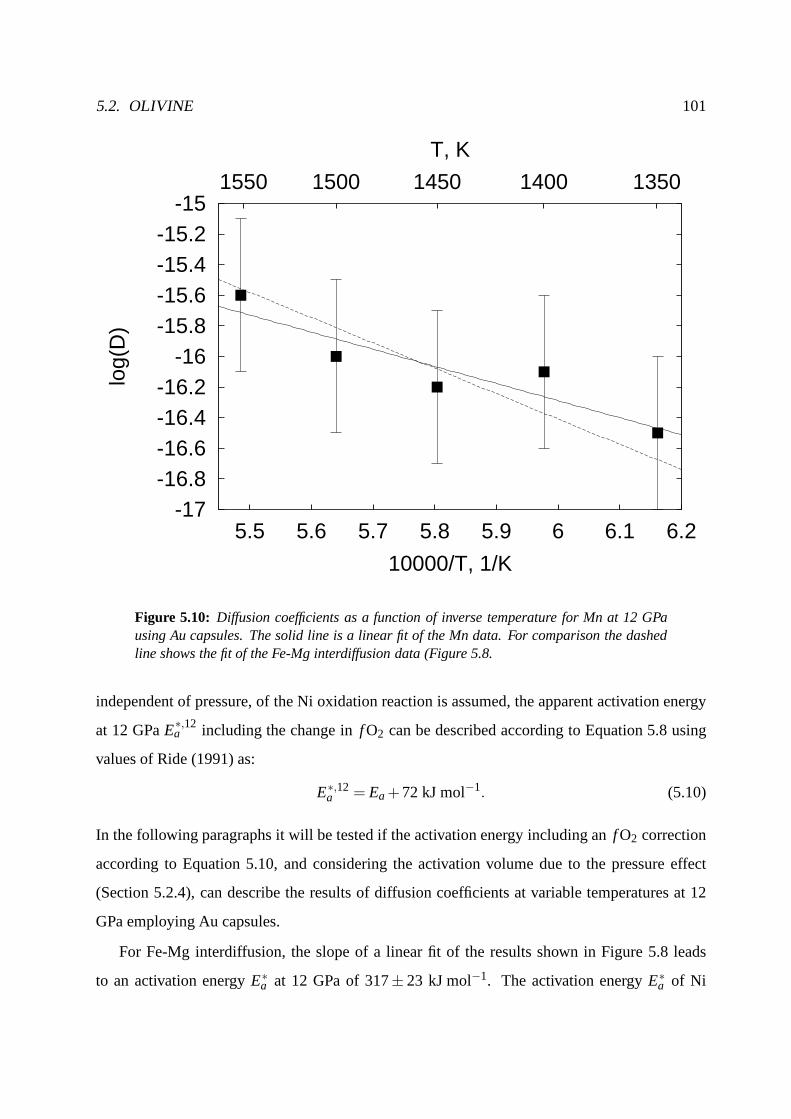
5.2. OLIVINE 101
-17-16.8-16.6-16.4-16.2
-16-15.8-15.6-15.4-15.2
-15
5.5 5.6 5.7 5.8 5.9 6 6.1 6.2
13501400145015001550
log(
D)
10000/T, 1/K
T, K
Figure 5.10: Diffusion coefficients as a function of inverse temperaturefor Mn at 12 GPausing Au capsules. The solid line is a linear fit of the Mn data.For comparison the dashedline shows the fit of the Fe-Mg interdiffusion data (Figure 5.8.
independent of pressure, of the Ni oxidation reaction is assumed, the apparent activation energy
at 12 GPaE∗,12a including the change inf O2 can be described according to Equation 5.8 using
values of Ride (1991) as:
E∗,12a = Ea+72 kJ mol−1. (5.10)
In the following paragraphs it will be tested if the activation energy including anf O2 correction
according to Equation 5.10, and considering the activationvolume due to the pressure effect
(Section 5.2.4), can describe the results of diffusion coefficients at variable temperatures at 12
GPa employing Au capsules.
For Fe-Mg interdiffusion, the slope of a linear fit of the results shown in Figure 5.8 leads
to an activation energyE∗a at 12 GPa of 317± 23 kJ mol−1. The activation energyE∗
a of Ni

102 CHAPTER 5. RESULTS
diffusion is 339±37 kJ mol−1 (determined using Figure 5.9) and for Mn diffusion a value of
214±55 kJ mol−1 (Figure 5.10) is derived. The errors correspond to the 1-σ standard deviation
of the linear fits. Considering the relatively small temperature range investigated, this error
slightly underestimates the true experimental error, as isevident by the fact that a change of 0.1
log units of the datapoint for Fe-Mg interdiffusion at 1623 Kchanges the value ofH∗a from 317
to 340 kJ mol−1. In addition, the fit of the Fe-Mg interdiffusion coefficients can relatively well
describe the Mn data within the error of the measurements (Figure 5.10), although the difference
in the best fit value ofE∗a between Fe-Mg interdiffusion and Mn diffusion is 100 kJ mol−1.
-17.2
-17
-16.8
-16.6
-16.4
-16.2
-16
-15.8
-15.6
-15.4
-15.2
-15
5.3 5.4 5.5 5.6 5.7 5.8 5.9 6 6.1 6.2 6.3
Log(
D/(
m2 s
ec-1
))
10000/T, 1/K
95% confidence bandEa
Ea + P ∆VaEa + P ∆Va + C(fO2)
Figure 5.11: 95% confidence bands for Fe-Mg interdiffusion (dashed lines). The solid lineis the linear fit of the data as described earlier in this section (page 101). The line labelledEa has a slope consistent with the 1 bar pressure activation energy. The other lines take thevariation of f O2 with pressure at constant temperture (Ea +P Va) and the variation of f O2with temperature at 12 GPa (Ea +P ∆Va +C( f O2) into account.
Figure 5.11 shows results of Fe-Mg interdiffusion coefficients at 12 GPa obtained using Au

5.2. OLIVINE 103
-17.5
-17
-16.5
-16
-15.5
-15
5.4 5.6 5.8 6 6.2
16231673172317731823
Log(
D/(
m2 s
ec-1
))
10000/T, 1/K
T, K
Fe-Mg interdiffusionNi diffusion
Mn diffusion
Figure 5.12: Superposition of results for Fe-Mg interdiffusion, Ni diffusion and Mn diffusion.
capsules together with the 95% lower and upper confidence bounds of a linear fit calculated with
the computer program MicrocalTMOriginTM (see also Sachs, 1997) superimposed. The solid line
is the linear fit obtained earlier (Figure 5.8). The line labelled Ea has a slope corresponding to the
1 bar value of 229 kJ mol−1 (Chakraborty, 1997). Considering the confidence bounds, the devi-
ation of this line from the best linear fit can still be interpreted by the error of the measurements
although the slope appears to underestimate the observed temperature dependence. To account
for the pressure effect, a termP×∆Va is added to the low pressure value (lineEa+P ∆Va in Fig-
ure 5.11), using the activation volume along the Ni-NiO buffer of∼ 5.5 cm3 mol−1 determined in
Section 5.2.4, hence including the variation inf O2 due to pressure at constant temperature. This
line is very close to the variation of log(D) versus inverse temperature observed in Figure 5.11.
If the oxygen fugacity inside the Au capsules would vary in the same way as the Ni-NiO buffer
then the contribution due to a change off O2 with temperature at 12 GPa has to be included in the

104 CHAPTER 5. RESULTS
activation energy (Equation 5.10, line termedEa+P ∆Va+C( f O2) in Figure 5.11). The slope of
this line is slightly higher than the linear best fit but stilldescribes the experimental results very
well considering the limits of the confidence bounds. This implies that within the error of the
experimental results, Fe-Mg interdiffusion coefficients determined using Au capsules, are very
close to conditions imposed by the Ni-NiO buffer in the experimental range of 1623 K to 1823
K at pressures between 6 and 12 GPa.
Figure 5.12 shows a superposition of results obtained for Fe-Mg interdiffusion, Ni diffusion
and Mn diffusion in order to compare the diffusvities of the different components to each other.
The data plotted in Figure 5.12 are overlapping to a large extent implying that within the tem-
perature interval investigated, diffusivities of divalent cations are very similar to each other as
already observed at 1 bar (Petry et al., 2003). Therefore, Fe-Mg interdiffusion coefficients can
be used as a proxy for divalent cation diffusion at high pressure in olivine.
5.2.6 Model of diffusion in olivine
In Section 5.2.4 the activation volume for Fe-Mg interdiffusion along the Ni-NiO buffer was
constrained to lie in the range of 5.1 to 6.1 cm3 mol−1. Therefore, a value of 5.6± 0.5 cm3
mol−1 is taken as the best fit value for the activation volume of Fe-Mg interdiffusion along the
Ni-NiO buffer. This value corresponds to a true activation volume of 7.4± 1.0 cm3 mol−1
at constant oxygen fugacity (Section 5.2.4), estimated using a model forf O2 as a function of
pressure with a constant volume change of the oxidation reaction of Ni. Combining these values
with existing results at 1 bar (Chakraborty, 1997, Dohmen, personal communication), allows to
formulate an Equation for Fe-Mg interdiffusion coefficients as function of pressure, temperature,
composition and oxygen fugacity in olivine along the c-axis:
DFe−Mg = 9.48×10⁻⁷ m2
sec( f O2)
15 exp
(
−229000+0.74P(bar)8.31441T(K)
)
exp(7 XFe2SiO4) . (5.11)
In Figure 5.13, Equation 5.11 is compared to Fe-Mg interdiffusion coefficients determined
at temperatures between 1623 K and 1823 K employing diffusion couples contained in Au cap-
sules at a pressure of 12 GPa. Within the error of the epxeriments a good consistency is observed.
Diffusion coefficients derived for Ni and Mn are very similarto values derived for Fe-Mg inter-
diffusion (Section 5.2.4, 5.2.5). Therefore, diffusion coefficients calculated using Equation 5.11

5.2. OLIVINE 105
-17-16.8-16.6-16.4-16.2
-16-15.8-15.6-15.4-15.2
-15
5.4 5.5 5.6 5.7 5.8 5.9 6 6.1 6.2
16231673172317731823
Log(
D/(
m2 s
ec-1
))
1/T, 1/K
T, K
global model
Figure 5.13: Fe-Mg interdiffusion coefficients are consistent with a model combining theactivation volume determined in this study with results at 1bar (Equation 5.11). See text forfurther details.
are very close to the diffusion coefficients of Ni and Mn at thesame conditions.
5.2.7 Comparison with previous results
The results for Fe-Mg interdiffusion obtained in this studyare shown together with literature
values of Misener (1974), Farber et al. (2000), and Chakraborty et al. (1999) in Figure 5.14.
Misener (1974) performed high pressure experiments up to 3.5 GPa in a piston cylinder ap-
paratus. Fe-Mg interdiffusion data at 1373 K andXFe2SiO4 = 0.4 were taken from Fig. 6 in
Misener (1974). A temperature correction to 1673 K employing an activation energy of 229 kJ
mol−1 (Chakraborty, 1997) was performed. The composition dependence was taken into account
with a correction of -1.0 log-units consistent with the correlation of diffusivity and composition
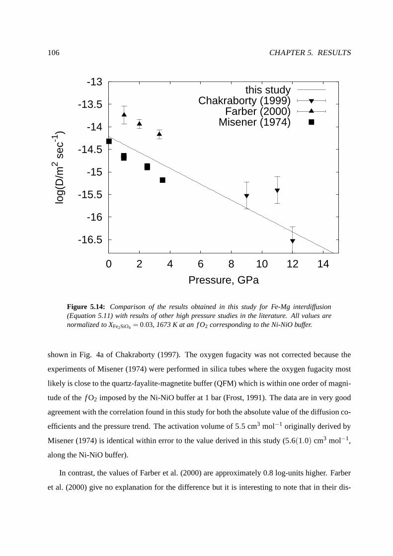
106 CHAPTER 5. RESULTS
-16.5
-16
-15.5
-15
-14.5
-14
-13.5
-13
0 2 4 6 8 10 12 14
log(
D/m
2 sec
-1)
Pressure, GPa
this studyChakraborty (1999)
Farber (2000)Misener (1974)
Figure 5.14: Comparison of the results obtained in this study for Fe-Mg interdiffusion(Equation 5.11) with results of other high pressure studiesin the literature. All values arenormalized to XFe2SiO4 = 0.03, 1673 K at an f O2 corresponding to the Ni-NiO buffer.
shown in Fig. 4a of Chakraborty (1997). The oxygen fugacity was not corrected because the
experiments of Misener (1974) were performed in silica tubes where the oxygen fugacity most
likely is close to the quartz-fayalite-magnetite buffer (QFM) which is within one order of magni-
tude of thef O2 imposed by the Ni-NiO buffer at 1 bar (Frost, 1991). The data are in very good
agreement with the correlation found in this study for both the absolute value of the diffusion co-
efficients and the pressure trend. The activation volume of 5.5 cm3 mol−1 originally derived by
Misener (1974) is identical within error to the value derived in this study (5.6(1.0) cm3 mol−1,
along the Ni-NiO buffer).
In contrast, the values of Farber et al. (2000) are approximately 0.8 log-units higher. Farber
et al. (2000) give no explanation for the difference but it isinteresting to note that in their dis-

5.2. OLIVINE 107
cussion they conclude that the results of Buening and Buseck(1973) are consistent with their
results although the diffusion coefficients of Buening and Buseck (1973) are almost an order of
magnitude faster. Hence, the establishement of consistency used in Farber et al. (2000) seems to
be rather ambiguous. In addition, the fact that the redox conditions prevailing in the experiments
of Misener (1974) are different than in Farber et al. (2000) is completely ignored in the discus-
sion of Farber et al. (2000). The water content of the diffusion couples of Farber et al. (2000)
was only established for the single crystals of olivine. More important would have been at least
a qualitative estimate of the water content of the polycrystalline parts of the experiments because
of possible water enrichment on the particle surfaces.
Partly, the difference between the results of this study andFarber et al. (2000), could be due
to grain boundary diffusion in the experiments of the latterwhich utilized a single crystal of
forsterite and polycrystalline fayalite as the diffusion couple. Based on estimates of the grain
boundary width in olivine and grain size, Farber et al. (2000) calculate that effective diffusion
coefficients (representing a combination of grain boundaryand bulk diffusion) might be up to 5
times greater than the true volume diffusion coefficient fortheir experiments. In addition, the
composition space investigated by Farber et al. (2000) comprises the whole compositional range
of XFe2SiO4 between 0 and 1. This might lead to some inaccuracies when calculating diffusivi-
ties at the more extreme ends of the diffusion couple. Because their values are all normalized
to XFe2SiO4 = 0.15, the diffusion coefficients were adjusted toXFe2SiO4 = 0.03 by substracting
0.5 log-units. The oxygen fugacity was close to the Ni-NiO buffer as in this study because
Ni containers with NiO were used. The experiments performedby Farber et al. (2000) for
Fe-Mg interdiffusion in olivine only span the pressure range up to 3.3 GPa. The pressure de-
pendence of Fe-Mg interdiffusion given in Farber et al. (2000) with an activation volume of
5.4(4.0) cm3 mol−1 along the Ni-NiO buffer is in good agreement with the resultspresented in
this work (5.6(1.0) cm3 mol−1).
In Chakraborty et al. (1999) three experiments performed inAu capsules using a similar as-
sembly to that employed in this study were reported. These experiments were performed at the
Bayerisches Geoinstitut using 1200 t multianvil press rather than the 500 t press used in this
study (see Section 2.2). The profile in Fig. 2A for olivine in Chakraborty et al. (1999) leads to

108 CHAPTER 5. RESULTS
a composition-dependent diffusion coefficient ofD = 2.2× 10⁻¹⁶exp(14.2 XFe2SiO4), reinves-
tigated with the numerical algorithm developed in Section 4.3.2. The composition dependence
is significantly stronger than observed at 1 bar as already noted in Chakraborty et al. (1999).
A closer investigation of one of their samples by EBSD revealed that only the Fe-rich olivine
was oriented along the c direction whereas the forsterite was oriented along the a axis generally
showing slower diffusion coefficients. From EBSD-mapping the change in orientation occurs
on a length scale below 1µm, implying no long range misorientation profiles. This explains the
strong asymmetry observed in the profiles of Chakraborty et al. (1999), although no kink in the
profile is observed. The comparison of data at 9, 11 and 12 GPa for Fe-Mg interdiffusion given
in Chakraborty et al. (1999) shows a good agreement with results of the present study although
interestingly the value at 11 GPa is again much faster than expected by a simple linear relation-
ship between logD and pressureP. The error bars were taken as large as in the present study
because the experimental procedure was the same in both setsof experiments.
It is difficult to compare the values of Jaoul et al. (1995), obtained between 0.5 and 9 GPa,
with the results reported here. In the present study, diffusion was determined in the c direction
whereas Jaoul et al. (1995) investigated diffusion along the b axis. The activation energy de-
rived is only 147 or 62 kJ mol−1, depending on the model describing the diffusion regime of
the experiments. It was claimed that these low activation energies are due to the experiments
being performed at low temperatures (873 K - 1173 K) in an extrinsic regime, whereas other
experiments at higher temperature would be in an intrinsic regime. The experiments of Buening
and Buseck (1973), from which a kink in the Arrhenius plot at 1373 K is observed, are taken as
evidence of this transition. This conclusion is contradicted by the conclusions of Chakraborty
(1997). According to his study, diffusion in Fe-bearing olivine occurs in laboratory experiments
always in a transition metal-extrinsic (TaMED) regime because diffusion rates depend on oxygen
fugacity (Section 1.2.3). The kink observed by Buening and Buseck (1973) is thus attributed to
the transition from a bulk to a grain boundary diffusion dominated regime. Hence, it is not clear
how to correct the data from Jaoul et al. (1995) to the high temperature conditions of this study
and they are thus omitted in Figure 5.14.
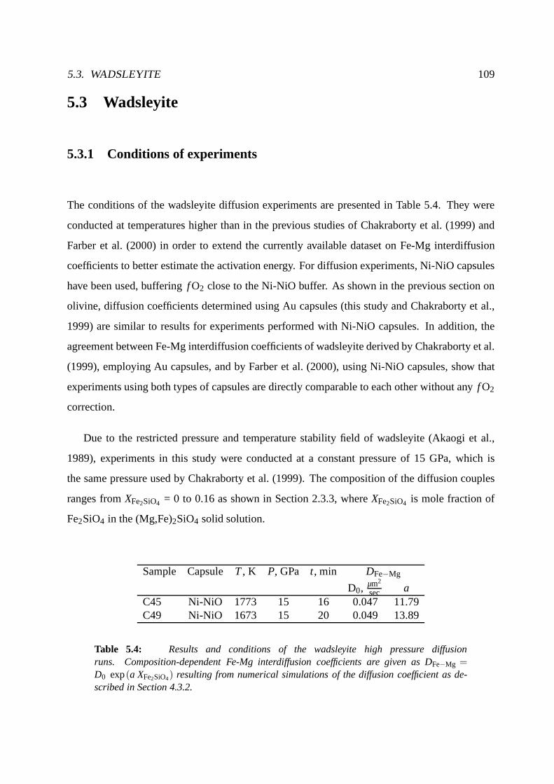
5.3. WADSLEYITE 109
5.3 Wadsleyite
5.3.1 Conditions of experiments
The conditions of the wadsleyite diffusion experiments arepresented in Table 5.4. They were
conducted at temperatures higher than in the previous studies of Chakraborty et al. (1999) and
Farber et al. (2000) in order to extend the currently available dataset on Fe-Mg interdiffusion
coefficients to better estimate the activation energy. For diffusion experiments, Ni-NiO capsules
have been used, bufferingf O2 close to the Ni-NiO buffer. As shown in the previous section on
olivine, diffusion coefficients determined using Au capsules (this study and Chakraborty et al.,
1999) are similar to results for experiments performed withNi-NiO capsules. In addition, the
agreement between Fe-Mg interdiffusion coefficients of wadsleyite derived by Chakraborty et al.
(1999), employing Au capsules, and by Farber et al. (2000), using Ni-NiO capsules, show that
experiments using both types of capsules are directly comparable to each other without anyf O2
correction.
Due to the restricted pressure and temperature stability field of wadsleyite (Akaogi et al.,
1989), experiments in this study were conducted at a constant pressure of 15 GPa, which is
the same pressure used by Chakraborty et al. (1999). The composition of the diffusion couples
ranges fromXFe2SiO4 = 0 to 0.16 as shown in Section 2.3.3, whereXFe2SiO4 is mole fraction of
Fe2SiO4 in the (Mg,Fe)2SiO4 solid solution.
Sample Capsule T, K P, GPa t, min DFe−Mg
D0, µm2
sec aC45 Ni-NiO 1773 15 16 0.047 11.79C49 Ni-NiO 1673 15 20 0.049 13.89
Table 5.4: Results and conditions of the wadsleyite high pressure diffusionruns. Composition-dependent Fe-Mg interdiffusion coefficients are given as DFe−Mg =D0 exp(a XFe2SiO4) resulting from numerical simulations of the diffusion coefficient as de-scribed in Section 4.3.2.
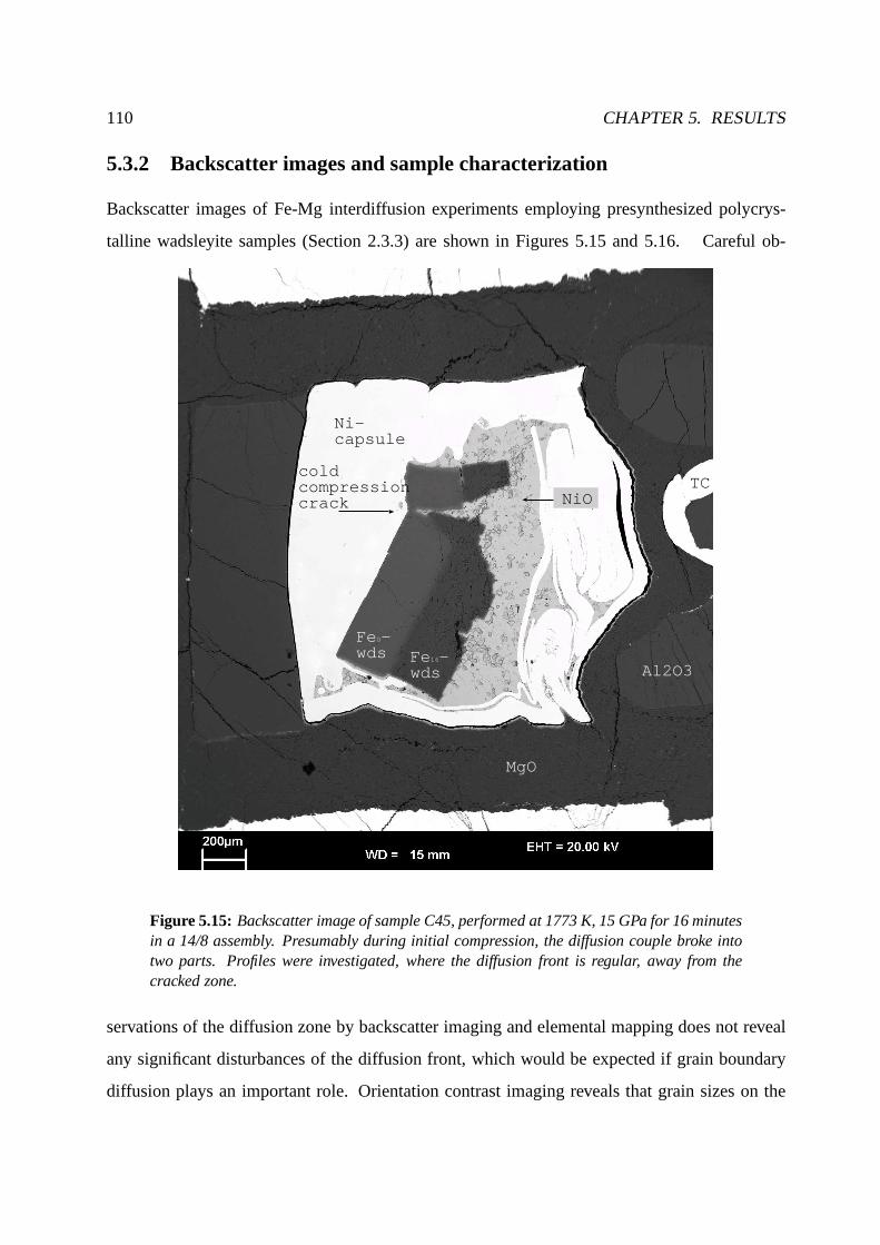
110 CHAPTER 5. RESULTS
5.3.2 Backscatter images and sample characterization
Backscatter images of Fe-Mg interdiffusion experiments employing presynthesized polycrys-
talline wadsleyite samples (Section 2.3.3) are shown in Figures 5.15 and 5.16. Careful ob-
Fe0-wds Fe16-
wds
Ni-capsule
NiO
MgO
TC
Al2O3
coldcompressioncrack
Figure 5.15: Backscatter image of sample C45, performed at 1773 K, 15 GPa for 16 minutesin a 14/8 assembly. Presumably during initial compression,the diffusion couple broke intotwo parts. Profiles were investigated, where the diffusion front is regular, away from thecracked zone.
servations of the diffusion zone by backscatter imaging andelemental mapping does not reveal
any significant disturbances of the diffusion front, which would be expected if grain boundary
diffusion plays an important role. Orientation contrast imaging reveals that grain sizes on the

5.3. WADSLEYITE 111
Rgw
(Mg1.68Fe0.32)SiO4-wds
(Mg2Fe0)SiO4-Wds
En
Nicapsule
NiO
Figure 5.16: Backscatter image of sample C49, performed at 1673 K, 15 GPa for 10 minutesin a 14/8 assembly. Wds denotes wadsleyite, Rgwd denotes ringwoodite, and En denotesenstatite.
Fe-rich side are on the order of 25µm. On the Mg-rich side, grains of approximately 60µm
are found which show a pervasive deformation microstructure. The large grains are recrystal-
lized into subgrains of∼ 1 µm during the high-pressure, high-temperature anneal. Potentially
this could lead to enhanced diffusion as was chown for the feldspar system by Yund and Tullis
(1991). Sometimes, diffusion along subgrain boundaries effects very short profiles (< 500 nm)
in perovskite diffusion experiments (see Section 5.5.3), but is probably not significant in the
wadsleyite experiments discussed here, as no effect is detected from element mapping.
The backscatter image of samples C45 and C49 (Figures 5.15 and 5.16), together with ele-
ment mapping, reveal the presence of a silica-rich phase with enstatite stoichiometry (hereafter
called enstatite), in addition to wadsleyite, on the Fe-free side of the interface. In this case this
phase is interpreted to result from the synthesis where the stoichiometry of the starting mixture
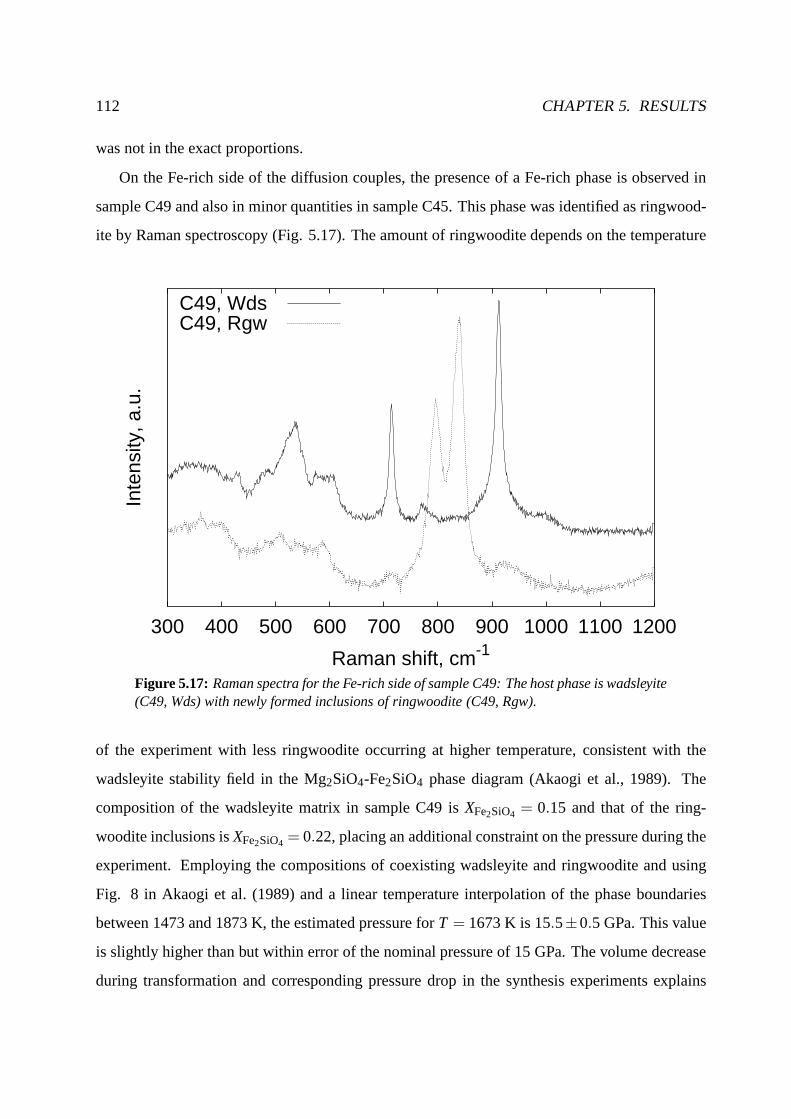
112 CHAPTER 5. RESULTS
was not in the exact proportions.
On the Fe-rich side of the diffusion couples, the presence ofa Fe-rich phase is observed in
sample C49 and also in minor quantities in sample C45. This phase was identified as ringwood-
ite by Raman spectroscopy (Fig. 5.17). The amount of ringwoodite depends on the temperature
300 400 500 600 700 800 900 1000 1100 1200
Inte
nsity
, a.u
.
Raman shift, cm-1
C49, WdsC49, Rgw
Figure 5.17: Raman spectra for the Fe-rich side of sample C49: The host phase is wadsleyite(C49, Wds) with newly formed inclusions of ringwoodite (C49, Rgw).
of the experiment with less ringwoodite occurring at highertemperature, consistent with the
wadsleyite stability field in the Mg2SiO4-Fe2SiO4 phase diagram (Akaogi et al., 1989). The
composition of the wadsleyite matrix in sample C49 isXFe2SiO4 = 0.15 and that of the ring-
woodite inclusions isXFe2SiO4 = 0.22, placing an additional constraint on the pressure duringthe
experiment. Employing the compositions of coexisting wadsleyite and ringwoodite and using
Fig. 8 in Akaogi et al. (1989) and a linear temperature interpolation of the phase boundaries
between 1473 and 1873 K, the estimated pressure forT = 1673 K is 15.5±0.5 GPa. This value
is slightly higher than but within error of the nominal pressure of 15 GPa. The volume decrease
during transformation and corresponding pressure drop in the synthesis experiments explains

5.3. WADSLEYITE 113
why ringwoodite inclusions are not evident in the synthesized samples prior to the diffusion
experiments.
Because wadsleyite can potentially accommodate several thousand ppm of water (Kohlstedt
et al., 1996; Bolfan-Casanova et al., 2000; Litasov and Ohtani, 2003), IR-spectroscopy was per-
formed on sample C45, resulting in water concentrations of around 35 ppm for both endmem-
bers (employing the absorption correction procedure of Paterson, 1982). This is an extremely
low water content for wadsleyite showing that the results presented here are representative of dry
wadsleyite. Preliminary results of Shimojuku et al. (2002)suggest that there may be a strong
influence of water on Fe-Mg interdiffusion in wadsleyite.
5.3.3 Profiles
Figures 5.18 and 5.19 show representative Fe and Mg concentration profiles for samples C45
0.75
0.8
0.85
0.9
0.95
1
500 520 540 560 580 600 620 640 6600
0.05
0.1
0.15
0.2
0.25
XM
g 2S
iO4
XF
e 2S
iO4
distance, µm
Fe
Mg
numerical simulation
Figure 5.18: Representative Fe and Mg profiles measured by EPMA on sample C45, per-formed at 15 GPa, 1773 K for 16 minutes.
and C49 (Table 5.4). Both profiles show a marked asymmetry, implying that the Fe-Mg interdif-

114 CHAPTER 5. RESULTS
0.75
0.8
0.85
0.9
0.95
1
0 50 100 150 200 250 300 350 4000
0.05
0.1
0.15
0.2
0.25
XM
g 2S
iO4
XF
e 2S
iO4
distance, µm
MgFe
simulation
Figure 5.19: Representative Fe and Mg profiles measured by EPMA on sample C49, per-formed at 15 GPa, 1673 K for 20 minutes. The large analytical scatter on the Fe-rich side ofthe profile results from the presence of inclusions of ringwoodite (see text), which are smallerthan the resolution limit of the profile analysis.
fusion coefficient is strongly composition-dependent. Hence, for retrieving diffusion coefficients
numerical simulations had to be performed, also shown in Fig. 5.18 and 5.19. It was found that
an exponential composition dependence, qualitatively valid also for olivine (Chakraborty, 1997),
well reproduces the observed asymmetrie of the profiles.
On the Fe-rich side of the profile shown in Figure 5.19 for experiment C49, performed at
15 GPa and 1673 K, the crystallization of ringwoodite, as described in the previous section,
causes the analytical scatter. For the simulation of the profile the composition of the wadsleyite
is taken for profile normalization (Section 4.1) and the ringwoodite is assumed to have formed
immediately after heating the experiment. This assumptionis justified because the wavelength
of the inclusions is roughly a factor of 10 smaller than the diffusion profile. Therefore, the time
of equilibration of the ringwoodite in the wadsleyite matrix should be approximately a factor of
100 faster than the establishment of the diffusion profile (estimated fromx ∝√
Dt, see Section

5.3. WADSLEYITE 115
4.2). In addition, because the crystallization of ringwoodite only occurred on the most Fe-rich
side of the diffusion couple, most of the profile length is notaffected. Hence, the role of ring-
woodite crystallization for the determination of diffusion coefficients should be negligible. Even
if the composition of the wadsleyite on the Fe-rich side changes during the diffusion experiment,
from XFe2SiO4 = 0.165, the average composition of the wadsleyite of sample C45which is al-
most unaffected by ringwoodite crystallization, toXFe2SiO4 = 0.153, the average wadsleyite com-
position of C49, the composition-dependent Fe-Mg interdiffusion coefficient would be between
4.9×10⁻¹⁴exp(12.96XFe2SiO4) m2 sec−1 and 4.9×10⁻¹⁴exp(13.89XFe2SiO4) m2 sec−1, result-
ing in a change of logDFe−Mg from -12.47 to -12.41 (forXFe2SiO4 = 0.15) at most. This is well
below the overall uncertainty of diffusion experiments in the multianvil apparatus, established for
the olivine experiments in Section 5.2.3. Therefore, absolute diffusivities determined for sam-
ple C49 were included for the determination of the activation energy (see Section 5.3.4). More
critial is the value in the exponent of the composition dependence. Because of a possible change
in the composition of the wadsleyite during the experiment (see above) and a higher dislocation
density in grains affected by ringwoodite crystallization(only for grains withXFe2SiO4 > 0.14)
this value might be slightly higher than the true value. Therefore, the composition dependence
determined for sample C45, is regarded as the best fit value for the composition dependence of
Fe-Mg interdiffusion in wadsleyite.
The relatively strong asymmetry of profiles observed in Fig.5.18 and 5.19 contrasts with the
symmetric profile shown for wadsleyite interdiffusion experiments in Fig. 2A of Chakraborty
et al. (1999). This difference results from the much smallercompositional range investigated by
Chakraborty et al. (1999) and is further investigated in thenext section, after establishing the
activation energy for Fe-Mg interdiffusion in wadsleyite.
5.3.4 Temperature dependence at 15 GPa
An Arrhenius plot showing the logarithm of the Fe-Mg interdiffusion coefficients logDFe−Mg
versus the inverse temperature, is given in Figure 5.20 withresults performed in this study and
Chakraborty et al. (1999). The experiments of Chakraborty et al. (1999), performed in Au cap-
sules, are believed to be at an oxygen fugacity close to the Ni-NiO buffer as the experiments

116 CHAPTER 5. RESULTS
-15
-14.5
-14
-13.5
-13
-12.5
-12
5.6 5.8 6 6.2 6.4 6.6 6.8 7 7.2 7.4
16731773 1573 1473 1373
this studyChakraborty (1999)
all data
Figure 5.20: Logarithm of the Fe-Mg interdiffusion coefficient for wadsleyite at 15 GPa as afunction of inverse temperature obtained in this study and by Chakraborty et al. (1999). Thedata of this study are recalculated to XFe2SiO4 = 0.14, the average composition of the earlierstudy of Chakraborty et al. (1999). As described in the text,the activation energy is derivedby fitting all data simultaneously.
in this study employing Ni capsules as discussed in Section 5.3.1. The diffusivities given in
Chakraborty et al. (1999), employing a composition-independent analytical solution to the dif-
fusion equation, Eq. 1.2, are representative ofXFe2SiO4 = 0.14, the average composition of their
diffusion couples. Thus values of this study were recalculated toXFe2SiO4 = 0.14 employing the
composition dependence given in Table 5.4 for the comparison shown in Figure 5.20.
The activation energy at 15 GPa,E15a = Ea + P× ∆Va, where∆Va is the activation vol-
ume along the Ni-NiO buffer, andEa is the activation energy at 1 bar, calculated from a
linear regression using the combined dataset of this study and Chakraborty et al. (1999) is
E15a = 260± 50 kJ mol−1, significantly larger than the preliminary estimate of 145 kJ mol−1
derived by Chakraborty et al. (1999). It should be emphasized that this activation energy was
determined along the Ni-NiO buffer and therefore also contains a contribution due to a change

5.3. WADSLEYITE 117
of f O2 with temperature at 15 GPa. The combined results of this study and of Chakraborty et al.
(1999) are in agreement with Farber et al. (2000) with respect to absolute diffusivities as shown
in Fig. 8 of Farber et al. (2000). It should be noted, that it isdifficult to understand the data
reduction scheme employed by Farber et al. (2000), because all data of Farber et al. (2000) are
recalculated toXMg = 0.85 as stated in the text, but at 10 GPa, and 1473 K ringwoodite is not sta-
ble but a spinel datapoint is listed in Table 1 of Farber et al.(2000) and plotted in their Figure 8.
Presumably diffusion coefficients were extrapolated across the phase boundary. A combined ac-
tivation volume is given for wadsleyite and ringwoodite together, employing only 1 datapoint for
wadsleyite. Hence, the determination of the activation volume in Farber et al. (2000) is question-
able. Therefore, for wadsleyite itself, no precise activation volume is available, and no pressure
correction of the activation energy was performed and the value of 260 kJ mol−1 is strictly only
valid at pressures of 15 GPa for oxygen fugacity conditions close to the Ni-NiO buffer.
In Section 5.3.2 it was reported that element mappings and backscattered electron images do
not reveal any grain boundary component. This is in agreement with the results of Chakraborty
et al. (1999) where a significant grain boundary contribution was observed at 1373 K, but not at
1473 K because the contribution of grain boundary diffusionbecomes smaller with increasing
temperature1.
The results obtained in this study for Fe-Mg interdiffusionin wadsleyite show an exponential
composition dependence which is stronger than observed forolivine (Table 5.4, Equation 5.11).
In order to test if the composition dependence observed in this study is compatible with the pro-
files measured by Chakraborty et al. (1999), simulations taking the value of the exponent of the
composition dependence of sample C45 (Table 5.4) and an preexponential factor consistent with
the average diffusion coefficient of 7×10⁻¹⁵ m2 sec−1 observed at 1473 K in Chakraborty et al.
(1999) were performed and compared to an example profile of sample H654, kindly provided by
S. Chakraborty in Figure 5.21. The simulated and measured profiles agree very well with each
other, implying that the composition dependence observed for a wider range of compositions
in this study is consistent with the results of Chakraborty et al. (1999), using a much smaller
1As evident in Figure 2 A of Chakraborty et al. (1999) the samples were switched in the original discussion.Sample H696, performed at 1373 K showed a significant contribution of grain boundary diffusion, whereas theprofiles of sample H654, performed at the higher temperatureof 1473 K result from lattice diffusion only.
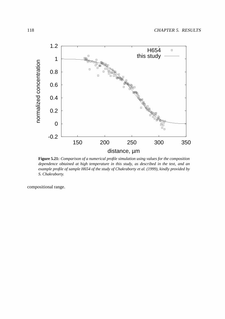
118 CHAPTER 5. RESULTS
-0.2
0
0.2
0.4
0.6
0.8
1
1.2
150 200 250 300 350
norm
aliz
ed c
once
ntra
tion
distance, µm
H654this study
Figure 5.21: Comparison of a numerical profile simulation using values for the compositiondependence obtained at high temperature in this study, as described in the text, and anexample profile of sample H654 of the study of Chakraborty et al. (1999), kindly provided byS. Chakraborty.
compositional range.

5.3. WADSLEYITE 119
5.3.5 Summary: Fe-Mg interdiffusion in wadsleyite
The preferred model for the Fe-Mg interdiffusion coefficient DFe−Mg in wadsleyite at 15 GPa,
along the Ni-NiO oxygen fugacity buffer, determined from the fit of all data shown in Fig. 5.20,
combined with the composition dependence obtained for sample C45, is:
DFe−Mg = (3.6±1.3)×10−6 exp((11.8±1.5) XFe2SiO4) exp
(
−260000±50000RT(K)
)
m2
sec.
(5.12)
Hence, the activation energy along the Ni-NiO oxygen fugacity buffer at 15 GPa for wadsleyite
has been shown to be 260 kJ mol−1 combining the data of this study and of Chakraborty et al.
(1999). This value is in much closer agreement with activation energies of “normal” silicates,
as the preliminary estimate of 145 kJ mol−1 determined earlier in Chakraborty et al. (1999). If
the activation energy is calculated on either dataset alone, the value is much different, showing
that for the determination of diffusional properties the range of conditions should be as large as
possible due to the relatively large uncertainties of high pressure diffusion experiments.
Figure 5.22 shows the difference in the Fe-Mg interdiffusions coefficient for olivine and
wadsleyite at the same temperature of 1673 K using Equations5.11 and 5.12. The difference is
roughly 4 orders of magnitude. This value is in agreement with Farber et al. (2000) and larger
than estimated in Chakraborty et al. (1999), because of the higher activation energy determined in
this study compared to the preliminary estimate of Chakraborty et al. (1999). This large change
in diffusivity across the olivine-wadsleyite phase boundary re-emphasizes the conclusions that
reequilibration becomes much faster in the transition zonethan in the upper mantle, originally
drawn by Chakraborty et al. (1999, see also Chapter 6).

120 CHAPTER 5. RESULTS
-18
-17
-16
-15
-14
-13
-12
0 2 4 6 8 10 12 14 16
Log(
D/(
m2 s
ec-1
))
Pressure, GPa
Ol, Eq. 5.7, XFe2SiO4 = 0.14
Wds, 1673 K, XFe2SiO4 = 0.14
Ol, this study, XFe2SiO4 = 0.03
Figure 5.22: Comparison of results of Fe-Mg interdiffusion experimentsemploying(Mg,Fe)2SiO4 olivine and wadsleyite solid solutions. Ol denotes olivineand Wds denoteswadsleyite. The value for olivine diffusion at 1 bar is takenfrom Chakraborty (1997).

5.4. FERROPERICLASE 121
5.4 Ferropericlase
5.4.1 Conditions of experiments
The initial compositions of the crystals and the experimental conditions are listed in Table 5.5.
The experiments were performed at temperatures between 1656 and 2073 K, at pressures be-
tween 8 and 23 GPa, and compositions ofXFeObetween 0.07 and 0.37, whereXFeOdenotes mole
fraction of FeO in (Mg,Fe)O. In addition, one experiment wasperformed where pure MgO (XFeO
= 0) was one endmember of the diffusion couple. This crystal had not been oriented previously
but otherwise prepared in a similar fashion to the Fe-bearing single crystals. For a characteriza-
tion of the crystals forming the diffusion couple see Section 2.3.4. All diffusion couples were
enclosed in Ni-NiO capsules for buffering thef O2 close to the Ni-NiO buffer (Section 2.4). At
pressures below 15 GPa a 14/8 assembly was used, whereas above 15 GPa a 10/4 assembly was
employed. For a description of the assemblies see Section 2.5.
The experiments were performed in the 1000 t or 1200 t press (Sections 2.2 and Appendix
A). For the short duration experiments (< 10 minutes annealing time), heating was performed
automatically with PID parameters of the Eurotherm temperature controller optimized in earlier
experiments. The proportionality band (P) was usually set to 2000%, the integral time (I) to
Table 5.5: Experimental conditions, initial compositions of diffusion couples, parametersD0, D1 and a for the equation D= (D0 + D1 · (XFeO)1.17) · exp(a·XFeO) (c.f. Eq. 1.16),and Fe-Mg interdiffusion coefficients for XFeO = 0.2. D1 was only fitted for sample C64 inwhich pure MgO was one end member. For all other results the power law contribution ofthe compositional dependence is not significant; D1 was therefore set to 0 (Eq. 1.17). Allvalues are averages of simulations of at least two profiles measured on each sample. As anexample Fe-Mg interdiffusion coefficients for XFeO = 0.2 are given in the last column.
Sample P, GPa T, K Assembly time, min XFeO XFeO D0, µm2
sec D1, µm2
sec a log(D/(m2 sec−1))crystal 1 crystal 2 XFeO= 0.2
C48 23 2063 10/4 40 0.079 0.363 0.037 0 7.23 -12.80C51 23 1851 10/4 183 0.080 0.370 0.0048 0 7.49 -13.67C53 23 1656 10/4 961 0.077 0.359 0.000454 0 6.82 -14.75C55 23 2073 10/4 21 0.079 0.362 0.035 0 7.38 -12.81C62 16 1873 10/4 45 0.082 0.356 0.053 0 7.54 -12.62C64 8 1873 14/8 20 0.00 0.354 0.0168 1.20 4.00 -12.35C67 8 1873 14/8 5 0.087 0.350 0.12 0 8.92 -12.15C68 12 1673 14/8 48 0.085 0.354 0.0063 0 10.66 -13.27C72 12 1873 14/8 20 0.077 0.335 0.042 0 8.87 -12.60C73 23 1923 10/4 46 0.082 0.340 0.028 0 7.41 -12.91C81 8 1873 14/8 15 0.086 0.363 0.132 0 8.66 -12.13
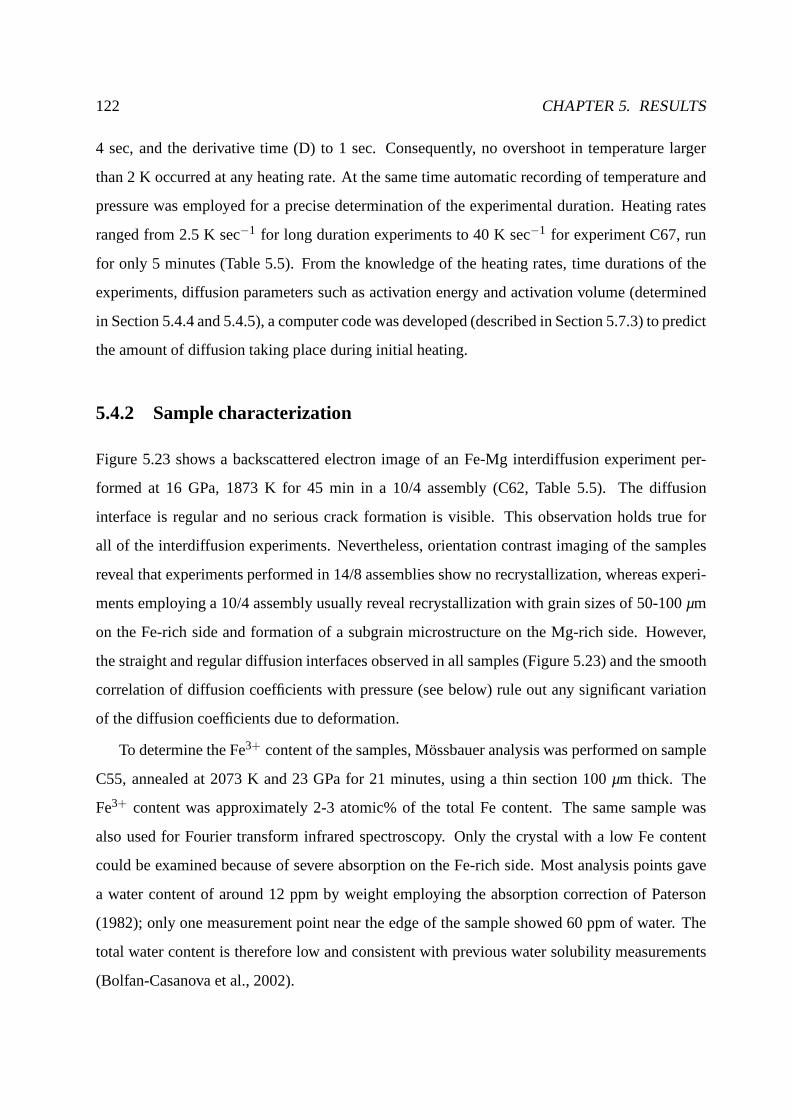
122 CHAPTER 5. RESULTS
4 sec, and the derivative time (D) to 1 sec. Consequently, no overshoot in temperature larger
than 2 K occurred at any heating rate. At the same time automatic recording of temperature and
pressure was employed for a precise determination of the experimental duration. Heating rates
ranged from 2.5 K sec−1 for long duration experiments to 40 K sec−1 for experiment C67, run
for only 5 minutes (Table 5.5). From the knowledge of the heating rates, time durations of the
experiments, diffusion parameters such as activation energy and activation volume (determined
in Section 5.4.4 and 5.4.5), a computer code was developed (described in Section 5.7.3) to predict
the amount of diffusion taking place during initial heating.
5.4.2 Sample characterization
Figure 5.23 shows a backscattered electron image of an Fe-Mginterdiffusion experiment per-
formed at 16 GPa, 1873 K for 45 min in a 10/4 assembly (C62, Table 5.5). The diffusion
interface is regular and no serious crack formation is visible. This observation holds true for
all of the interdiffusion experiments. Nevertheless, orientation contrast imaging of the samples
reveal that experiments performed in 14/8 assemblies show no recrystallization, whereas experi-
ments employing a 10/4 assembly usually reveal recrystallization with grain sizes of 50-100µm
on the Fe-rich side and formation of a subgrain microstructure on the Mg-rich side. However,
the straight and regular diffusion interfaces observed in all samples (Figure 5.23) and the smooth
correlation of diffusion coefficients with pressure (see below) rule out any significant variation
of the diffusion coefficients due to deformation.
To determine the Fe3+ content of the samples, Mossbauer analysis was performed on sample
C55, annealed at 2073 K and 23 GPa for 21 minutes, using a thin section 100µm thick. The
Fe3+ content was approximately 2-3 atomic% of the total Fe content. The same sample was
also used for Fourier transform infrared spectroscopy. Only the crystal with a low Fe content
could be examined because of severe absorption on the Fe-rich side. Most analysis points gave
a water content of around 12 ppm by weight employing the absorption correction of Paterson
(1982); only one measurement point near the edge of the sample showed 60 ppm of water. The
total water content is therefore low and consistent with previous water solubility measurements
(Bolfan-Casanova et al., 2002).

5.4. FERROPERICLASE 123
MgO
LaCrO
3 (furnace)
Ni
NiO
(Mg92Fe8)O
(Mg63Fe37)O
TC
ZrO2
ZrO2
LaCrO
3 (furnace)
Figure 5.23: Backscattered electron image of the pressure assembly after a ferropericlasediffusion experiment. Conditions of the experiment were 16GPa and 1873 K with an an-nealing time of 45 min. The diffusion couple is seen surrounded by the Ni capsule. The NiOused for buffering f O2 also interacted chemically with the end of the diffusion couple over adistance of∼ 150µm
5.4.3 Profiles and diffusion coefficients
Profiles of Fe and Mg in ferropericlase are strongly asymmetric as shown by an example of an
experiment performed at 8 GPa, 1873 K for 15 minutes in a 14/8 assembly in Figure 5.24. The
lengths of the profiles, measured on different samples, range between 80 and 230µm. Hence,
diffusion profiles can be easily investigated by EPMA. For deriving the composition-dependent
diffusion coefficient, both methods described in Section 4.3, Boltzmann-Matano analysis (BMA)
and the numerical finite difference method (FDM), were applied. A comparison of diffusion
coefficients derived using both methods is given in Figure 5.25. The numerical simulation very
precisely reproduces the asymmetry of the profile whereas the fitting function fails to adequately

124 CHAPTER 5. RESULTS
0.6
0.65
0.7
0.75
0.8
0.85
0.9
0.95
100 150 200 250 300 350 4000.05
0.1
0.15
0.2
0.25
0.3
0.35
0.4
XM
gO
XF
eO
distance, µm
MgFe
simulation
Figure 5.24: Fe and Mg profiles for sample C81, performed at 8 GPa, 1873 K for15 min.XMgO,FeOdenotes mole fraction of FeO or MgO. Also shown is a profile simulation employinga finite difference algorithm (see text and Section 4.3.2)
describe the profile at very low and very high Fe contents. Presumably this happens because the
middle part of the profiles contributes more to the sum of squared deviations minimized during
the least square nonlinear fit of the fitting function. This holds true for all fitting function types
described in Section 4.3.1. The fitting might be also problematic because of the high nonlinearity
of the fitting functions. Hence, the detection of the global minimum becomes difficult. As a
consequence diffusion coefficients derived by BMA and by FDMagree very well at intermediate
compositions whereas at the extreme ends of the profile a systematic deviation of∼ 0.1 log-
unit was observed (inset of Figure 5.25). Based on these comparisons, all diffusion coefficients
reported for ferropericlase were derived by FDM and fitted parameters for the constantsD0 and
a in Eq. 1.17 are also listed in Table 5.5.
For sample C64, in which an MgO single crystal was used as one end member, the nu-
merical model, using only an exponential composition dependence (Equation 1.17), slightly

5.4. FERROPERICLASE 125
0
0.2
0.4
0.6
0.8
1
20 40 60 80 100 120 140 160 180 200
norm
alis
ed c
once
ntra
tion
distance, µm
Richards-fit:C(x)=P1/(P2+e(x-P3)·P4)P5
numericalsimulation
-13.9
-13.7
-13.5
-13.3
0.1 0.3 0.5 0.7 0.9
log(
D/m
2 /sec
)
normalised composition
Composition dependence
exponential dependence
from
Boltzmann-
Matano
analysis
Figure 5.25: Comparison of diffusion coefficients derived by Boltzmann-Matano analysisand finite difference simulations for sample C51 (Table 5.5). The profile is shown onto whichthe fitting function for the Boltzmann-Matano analysis and the results of the numerical sim-ulation are superimposed. The inset shows the logarithm of the diffusion coefficient as afunction of normalized Fe-content.
overestimates diffusivities at the MgO-rich end of the profile (Figure 5.26). In this region the
composition power law dependence contributes significantly to the diffusivity (see Eq. 1.16 and
Mackwell et al., 2004). This implies a change in the charge neutrality condition for point defects
when approaching the MgO rich end of the solid solution. Therefore the profiles for this sample
were reanalyzed with a composition dependence ofD =(
D0 +D1 · (XFeO)1.17)
· exp(a ·XFeO)
(cf. Eq. 1.16), where the constanta was fixed at a constant value of 4, consistent with the results
at 1 bar (Mackwell et al., 2004), and the constantsD0 andD1 were allowed to vary. The result
of this simulation is also given in Table 5.5. The details of this simulation are further described
in Appendix C.
To test the inter-experiment reproducibility a time seriesof experiments was performed at
constant temperature of 1873 K and constant pressure of 8 GPa(Fig. 5.27). The three experi-

126 CHAPTER 5. RESULTS
Figure 5.26: Fe profile measured on sample C64, performed at 8 GPa, 1873 K, for 20minutes employing a diffusion couple of0 < XFeO < 0.35 (see Table 5.5). The inset showsthe region of low Fe concentrations, where a simulation witha pure exponential compositiondependence of the diffusion coefficient (Exp) does not adequately reproduce the profile anda simulation with a power law dependence in the preexponential factor (PL + Exp) had tobe employed (see Equations 1.16 and 1.17 and text for furtherexplanations).
ments were performed for 5, 15 and 20 minutes using differentheating rates, multianvil presses
and types of diffusion couples as indicated in Figure 5.27. No systematic variation of diffusivity
as a function of time was observed and the overall scatter of the data was found to be better than
± 0.3 log-units. Therefore, at these conditions no zero-time effect due to heating was observed
experimentally.

5.4. FERROPERICLASE 127
-13.5
-13
-12.5
-12
-11.5
-11
-10.5
0 5 10 15 20 25
logD
(m2 /s
ec)
time, minutes
XFeO = 0.3
XFeO = 0.1
C641000 t presshr: 3.3 K/secXFeO(DC):0-0.355
C671200 t presshr: 40 K/secXFeO(DC):0.087-0.350
C811000 t presshr: 10 K/secXFeO(DC):0.086-0.363
Figure 5.27: Logarithm of the diffusion coefficient at constant temperature of 1873 K andconstant pressure of 8 GPa. The dashed lines show the averagevalues of diffusivity, recalcu-lated for XFeO = 0.1 and 0.3. The time series shows that the effects of the variation of heatingrate (hr), multianvil press (1000 t or 1200 t), and compositions of the diffusion couples (DC)on the results are negligible.

128 CHAPTER 5. RESULTS
5.4.4 Pressure dependence at constant temperature
The composition-dependent Fe-Mg interdiffusion coefficient D at high pressure can be described
by:
D = D0 ·exp
(
A ·XFeO
R·T
)
·exp
(
−Ea +(P−Pre f ) ·∆Va
R·T
)
(5.13)
where the constantA describes the compositional dependence,XFeO is the mole fraction of FeO,
∆Va is the activation volume,Ea is the activation energy,P is the pressure,Pre f is the reference
pressure (= 1bar), andT is absolute temperature (compare with Equations 1.14 and 1.16). As
discussed by Poirier (2000) the pressure dependence of the entropic term is neglected in this
formulation. Equation 5.13 is consistent with Eq. 1.16, derived from point defect considerations,
as long asXFeO> 0.07 (see Section 1.3.2). Strictly, Equation 5.13 is only valid at constant oxygen
fugacity. Because the experiments of this study were performed at oxygen fugacity conditions
close to the Ni-NiO buffer, values derived later for the activation energy and the activation volume
will also include a contribution due to change inf O2.
Figures 5.28 and 5.29 show the pressure dependence of diffusion from which the value of
the activation volume∆VA (Eq. 5.13) has been determined using the slope of a linear regres-
sion. Diffusivities at different compositions were calculated for each experiment by using the
constantsa andD0 in Eq. 1.17 listed in Table 5.5. The constanta in Eq. 1.17 corresponds to
A/(R ·T) in Eq. 5.13. At 23 GPa, Fe-Mg interdiffusion coefficients were recalculated to 1673
K and 1873 K using the temperature dependence given in Fig. 5.30. At 8 GPa and 1873 K
three experiments have been performed, one of them using a diffusion couple of a pure MgO
single crystal as one endmember (C64 - Table 5.5) and two employing a diffusion couple with
XFeO= 0.09 andXFeO= 0.35 (C67, C81). No significant differences in the diffusion coefficients
derived using the different kinds of diffusion couples are observed (Fig. 5.27). Hence the result
from C64 was included in all calculations presented below. From Fig. 5.28 values for the activa-
tion volume of 3.4±0.5 and 3.3±0.5 cm3 mol−1 at 1673 and 1873 K respectively are evaluated
from the slopes of the regression lines. Figure 5.29 shows that at 1873 K the activation volume is
3.0±0.5 cm3 mol−1 atXFeO= 0.1, 3.3±0.5 cm3 mol−1 atXFeO= 0.2, and 3.5±0.5 cm3 mol−1
at XFeO= 0.1. The error on the activation volume was estimated from the 1sigma standard de-
viation of the fit of logD versus pressure at a fixed temperature and composition. Because the

5.4. FERROPERICLASE 129
-15
-14.5
-14
-13.5
-13
-12.5
-12
-11.5
-11
-10.5
0 5 10 15 20 25
LogD
(m2 /s
)
Pressure, GPa
XFeO = 0.2
1673 K 1873 K
individual fit at 1673 K and 1873 Kglobal fit at 1673 K and 1873 K
Figure 5.28: Pressure dependence of diffusivity at 1673 K and 1873 K and a constant com-position of XFeO = 0.2 (using data from Table 5.5). Data at 1 bar are from Mackwell et al.(2004). At 23 GPa, data-points are recalculated to 1673 K and1873 K from the correlationshown in Figure 5.30. Individual fits to the datapoints at each temperature, calculated usingvalues from Table 5.5, are shown by the solid lines. The dotted lines show a global fit of Eq.5.13 with the parameter values detailed in the text.
total variation is not larger than the 1 sigma standard deviation, it is concluded that at the exper-
imental conditions the activation volume does not depend significantly on either temperature or
composition.
5.4.5 Temperature dependence at constant pressure
Figure 5.30 shows an Arrhenius diagram for ferropericlase diffusion coefficients at 23 GPa. In
the case of ferropericlase, where the diffusion coefficientdepends on concentration as given in
Equation 5.13, the slope in the Arrhenius diagram is−(Ea−A XFeO+∆Va (P−Pre f)/(2.3026 R)
(see also Figure 1.1). The activation energyEa at 23 GPa can be determined using the calculated
activation volumeVa and the average constantA determined using Table 5.5 whereA(Eq. 5.13) =
a(Tbl. 5.5, Eq. 1.17)×RT, which at 23 GPa is 1.16×10⁵ J mol−1, from a plot of logD against
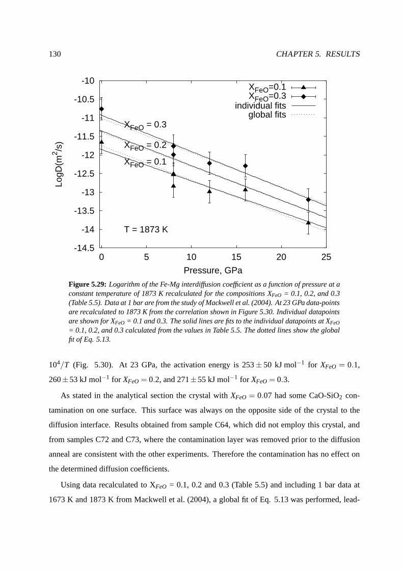
130 CHAPTER 5. RESULTS
-14.5
-14
-13.5
-13
-12.5
-12
-11.5
-11
-10.5
-10
0 5 10 15 20 25
LogD
(m2 /s
)
Pressure, GPa
T = 1873 K
XFeO = 0.1
XFeO = 0.2
XFeO = 0.3
XFeO=0.1XFeO=0.3
individual fitsglobal fits
Figure 5.29: Logarithm of the Fe-Mg interdiffusion coefficient as a function of pressure at aconstant temperature of 1873 K recalculated for the compositions XFeO = 0.1, 0.2, and 0.3(Table 5.5). Data at 1 bar are from the study of Mackwell et al.(2004). At 23 GPa data-pointsare recalculated to 1873 K from the correlation shown in Figure 5.30. Individual datapointsare shown for XFeO = 0.1 and 0.3. The solid lines are fits to the individual datapoints at XFeO
= 0.1, 0.2, and 0.3 calculated from the values in Table 5.5. The dotted lines show the globalfit of Eq. 5.13.
104/T (Fig. 5.30). At 23 GPa, the activation energy is 253± 50 kJ mol−1 for XFeO = 0.1,
260±53 kJ mol−1 for XFeO= 0.2, and 271±55 kJ mol−1 for XFeO= 0.3.
As stated in the analytical section the crystal withXFeO = 0.07 had some CaO-SiO2 con-
tamination on one surface. This surface was always on the opposite side of the crystal to the
diffusion interface. Results obtained from sample C64, which did not employ this crystal, and
from samples C72 and C73, where the contamination layer was removed prior to the diffusion
anneal are consistent with the other experiments. Therefore the contamination has no effect on
the determined diffusion coefficients.
Using data recalculated to XFeO = 0.1, 0.2 and 0.3 (Table 5.5) and including 1 bar data at
1673 K and 1873 K from Mackwell et al. (2004), a global fit of Eq.5.13 was performed, lead-

5.4. FERROPERICLASE 131
-15.5
-15
-14.5
-14
-13.5
-13
-12.5
-12
4.8 5 5.2 5.4 5.6 5.8 6 6.2
16731773187319732073
LogD
(m2 /s
)
10000/T, 1/K
Temperature, K
P = 23 GPa
XFeO = 0.1
XFeO = 0.2
XFeO = 0.3
XFeO = 0.1XFeO = 0.3
individual fitsglobal fit
Figure 5.30: Logarithm of the diffusion coefficient as a function of inverse temperature.Individual datapoints, recalculated for XFeO = 0.1 and 0.3 using parameters listed in Table5.5, are shown for experiments performed at 23 GPa and 1656 - 2073 K. In addition, forXFeO = 0.1, 0.2, and 0.3, individual fits of the datapoints at theseconditions are shown bythe solid lines. At the same conditions the results of the global fit (Eq. 5.13) are shown bythe dotted lines.
ing to A = 132± 13 kJ mol−1, activation energyEa = 255± 16 kJ mol−1, activation volume
∆Va = 3.3±0.1 cm3 mol−1, and the preexponential factorD0 = (9.8±0.7)×10−6 m2 sec−1.
The quoted errors are standard errors from the Mathematica (Version 4.1.0.0, Wolfram Research)
package LinearRegression. From the deviation of the calculated and experimentally determined
values the overall error is estimated to be 0.3 log-units. These values for Eq. 5.13 are valid for
an oxygen fugacity corresponding to the Ni-NiO-buffer as discussed in Section 5.1. The experi-
mental conditions for deriving these parameters were pressures of 0 - 23 GPa and temperatures
of 1656 - 2073 K.
The value of 3.3 cm3 mol−1 is in good agreement with the activation volume of 3.0
cm3 mol−1 determined for Mg tracer diffusion in the experiments of VanOrman et al. (2003).

132 CHAPTER 5. RESULTS
5.4.6 Oxygen fugacity
All experiments reported here have been performed in Ni capsules in contact with NiO powder
(Fig. 5.23). Therefore Eq. 5.13 is only valid at oxygen fugacities corresponding to the Ni-NiO
buffer. Because fO2 at the Ni-NiO buffer varies with temperature and pressure, this dependence
is implicitly built into Eq. 5.13 (Section 5.1).
According to Mackwell et al. (2004), Fe-Mg interdiffusion in ferropericlase varies with fO2
by the factor of (fO2)0.22. To test if the high-pressure, high-temperature dependence of Fe-Mg
interdiffusion is independently consistent with the 1 bar data from Mackwell et al. (2004), Eq.
5.13 was refitted without including the 1 bar data. The difference between diffusivities calculated
at 1 bar using the back extrapolation of the high pressure data, and those calculated from the
results of Mackwell et al. (2004) at an fO2 corresponding to the Ni-NiO buffer, ranges from 0.01
log units at 1673 K andXFeO = 0.1 to 0.58 log units at 2073 K forXFeO = 0.3. Considering the
experimental error of 0.3 log-units and the fact that the experimental data are extrapolated over a
pressure range of 8 GPa, these differences indicate good consistency between the high pressure
results and data obtained at 1 bar.
The results of a similar fit as in the previous section but including f O2 values calculated using
data of Ride (1991) is presented in the next section.
5.4.7 Summary: Ferropericlase
Fe-Mg interdiffusion in ferropericlase has been studied atpressures between 8 and 23 GPa and
temperatures between 1653 K and 2073 K, using a multianvil apparatus. The compositions of
the single crystal diffusion couples wereXFeO = 0.07 for one crystal andXFeO = 0.37 for the
other, although in one case pure MgO was used instead ofXFeO= 0.07. Fe-Mg interdiffusion at
oxygen fugacities buffered by Ni-NiO, including 1 bar data at 1673 K and 1873 K of Mackwell
et al. (2004), can be described for 0.07< XFeO < 0.37 by:
DFe−Mg = 9.9(±0.7)×10−6 exp
(
132000(±13000) XFeO
8.31441T(K)
)
·
exp
(
−255000(±16000)+0.33(±0.01) P(bar)8.31441T(K)
)
m2
sec. (5.14)

5.4. FERROPERICLASE 133
These results will be used in Section 6.2.1 to constrain Fe-Mg interdiffusion coefficients of fer-
ropericlase in the Earth’s lower mantle.
In addition to the fit of results corresponding to an oxygen fugacity of the Ni-NiO buffer,
values for the activation energy and the activation volume were also derived for constantf O2.
For this purpose, the absolute oxygen fugacity of the experiments was calculated using values
given in Ride (1991), as discussed in Section 5.1. The results of this recalculation depend on
the f O2 exponent of the oxygen fugacity dependence of the Fe-Mg interdiffusion coefficient
(e.g. Equation 1.6). In Section 1.2.4 an exponent of 1/6 was derived for a vacancy mechanism
of diffusion. In this case the activation volume is 4.8 cm3 mol−1 and the activation energy
becomes 178 kJ mol−1. Mackwell et al. (2004) derived an experimental value of 1/4.5 for the
f O2 exponent (Equation 1.16) leading to an activation volume of5.2 cm3 mol−1 and an activation
energy of 153 kJ mol−1 at constant oxygen fugacity. In both cases, the value of the activation
energy is significantly smaller than the 1 bar value of 206500J mol−1 (Mackwell et al., 2004).
Therefore, it is concluded that the temperature dependenceof the oxygen fugacity of the Ni-NiO
buffer is not accurately predicted at pressures up to 23 GPa using existing data for the Ni-NiO
buffer obtained at 1 bar and pressures below 4.5 GPa.
In a recent paper by Yamazaki and Irifune (2003) Fe-Mg interdiffusion in ferropericlase was
studied between 7 and 35 GPa. These authors found absolute diffusivities similar to the values
observed in this study but the pressure trend was much weakerresulting in an activation volume
of 1.8 cm3 mol−1. For experiments up to 28 GPa Yamazaki and Irifune (2003) used Re capsules
and assumed that the oxygen fugacity is close to the Re-ReO2 buffer. Although it was shown by
Frost and Langenhorst (2002) that this is a reasonable assumption at pressure of approximately
24 GPa, the data of Yamazaki and Irifune (2003) indicate thatthis assumption does not hold
true at lower pressures. The Fe-Mg interdiffusion coefficient at 1 bar consistent with an oxygen
fugacity of the Re-ReO2 buffer is 5.3×10⁻¹² m2 sec−1 using values of Mackwell et al. (2004,
see also Section 1.3.2), which is more than a factor of 10 larger than calculated using the model
of Yamazaki and Irifune (2003). Hence, the oxygen fugacity inside the Re capsules used by
Yamazaki and Irifune (2003) changes from reducing conditions well below the Ni-NiO buffer
at 1 bar to oxidizing conditions consistent with the Re-ReO2 buffer at pressures of∼ 25 GPa.

134 CHAPTER 5. RESULTS
Therefore, a completely different variation in diffusivity due to a change inf O2 with pressure is
built into the apparent activation volume determined by Yamazaki and Irifune (2003) compared
to the results of this study and consequently the activationvolumes determined in both studies
cannot be compared directly to each other.
5.5. (FEXMG1−X)SIO3 PEROVSKITE 135
5.5 (FexMg1−x)SiO3 Perovskite
5.5.1 Introduction, conditions of experiments
The conditions of all experiments are summarized in Table 5.6. Experiments were performed at
temperatures between 1973 K and 2273 K at pressures in the range of 22 to 26 GPa, employing
diffusion couples in MgO-Fe and Ni-NiO capsules (Section 2.4). High temperature runs (> 2173
K) were performed in the 5000 t press using an 18/8 assembly inorder to achieve a better temper-
ature stability. However, the absolute pressure in this assembly is smaller compared to the 10/4
assembly, as revealed by partial back-transformation of perovskite to majorite (Section 5.5.2).
Because of the higher pressures in the 10/4 assembly employed in the 1000 t and 1200 t presses,
the pressure of the experiments varies slightly between 22-26 GPa (Table 5.6), depending on the
press and assembly used. When comparing diffusivities of perovskite determined using different
presses and assemblies in latter sections no pressure normalization was employed because the
activation volume of Fe-Mg interdiffusion in silicate perovskite is unknown. The resulting dif-
ference in diffusivity due to a pressure variation of 4 GPa would be on the order of 0.5 log-units,
assuming a typical activation volume for silicates of 5 cm3 mol−1 (e.g. in olivine).
The diffusion couples used for the perovskite diffusion experiments consisted of pure presyn-
thesized MgSiO3 perovskite and Fe bearing samples synthesized prior the diffusion experiments
employing either synthetic polycrystalline enstatite or anatural single crystal bronzite as dis-
cussed in Section 2.3.5. For the high pressure diffusion anneal, the diffusion couples were en-
closed either by MgO-Fe capsules (Section 2.4) for buffering the oxygen fugacity at reducing
conditions or by Ni-NiO capsules (Section 2.4) for attaining more oxidizing conditions.
5.5.2 SEM and EPMA investigations of perovskite diffusion experiments
After the high pressure experiments, samples were mounted in epoxy and polished until the mid-
dle of the diffusion couple was exposed (Figure 3.1). Phaseswere identified using Raman spec-
troscopy. For all experiments performed in the 10/4 assembly the perovskite was well preserved.
In the 18/8 assembly, employing only MgO-Fe capsules, the perovskite adjacent to the metal was
transformed to majorite consuming half of the original perovskite in sample C30 (Table 5.6).
Figure 5.31 shows backscatter electron images of diffusionexperiments performed in MgO-

136 CHAPTER 5. RESULTS
MgSiO3 perovskite
(Mg,Fe)SiO3 perovskite
Fe
MgOA
MgSiO3 perovskite
(Mg,Fe)SiO3 perovskite
MgO-capsule
Fe
Ringwoodite layerMgO-capsule
Majorite
B
microprobetraverses
Figure 5.31: Backscattered electron images of perovskite diffusion couples performed inMgO-Fe capsules. The experiment in A was run at 25 GPa, 2073 K for 240 min employinga 10/4 assembly, the experiment in B was run at 22 GPa, 2273 K for 373 min using an 18/8assembly.

5.5. (FEXMG1−X)SIO3 PEROVSKITE 137
Table 5.6: Conditions of the perovskite diffusion experiments. P is sample pressure, T issample temperature as indicated by the thermocouple or estimated by the power reading(only C76), t is the duration of the experiment at high temperature, capsule is the capsuletype (Section 2.4), XFeO is the mole fraction of FeO in the rim of the MgO capsule for ex-periments performed in MgO-Fe capsules, and∆ f O2 is the oxygen fugacity relative to theiron-wustite buffer defined in Eq. 5.19 and calculated by assuming ideality in Eq. 5.20 (onlyfor experiments performed in MgO-Fe capsules).
Sample press P, GPa T, K t, min capsule XFeO ∆ f O2
C13 Sumitomo 24 2043 240 MgO-Fe 0.069 -2.33C19 Hymag 24 2023 483 MgO-Fe 0.027 -3.14C22 Hymag 24 2073 900 MgO-Fe 0.035 -2.91C23 Hymag 24 2123 720 MgO-Fe 0.022 -3.33C28 Hymag 24 2133 1430 MgO-Fe 0.048 -2.64C30 Zwick 22 2273 373 MgO-Fe 0.116 -1.87C61 Hymag 26 2073 10 Ni-NiOC70 Hymag 26 2173 60 Ni-NiOC76 Hymag 26 1973 570 Ni-NiO
Fe capsules. Fig. 5.31-A shows a cross section of an experiment at 25 GPa, 2073 K run for 240
min in the 1000 t (Hymag) press employing a 10/4 assembly, whereas in Fig. 5.31-B a cross
section of a sample at 22 GPa, 2273 K run for 373 min in the 5000 t(Zwick) press employing
an 18/8 assembly is shown. In most cases the iron shows structures indicative of melting like
intrusion along grain boundaries of the capsule and betweencapsule and sample but not in the
polycrystalline perovskite diffusion couple (Figure 5.31-B). Stishovite crystals and iron oxides
are often found in the metal. In the 10/4 assembly in most experiments a perovskite reaction
rim is observed adjacent to the MgO of the capsule which is interpreted as reaction of SiO2
dissolved in the metal with the MgO during quench. Because pressures in the 18/8 assembly are
significantly lower, reaction rims observed adjacent to theMgO consists of ringwoodite in this
case (Figure 5.31-B). At the same time, for experiment C30 (Table 5.6) performed in an 18/8
assembly, the perovskite is partially consumed and majorite formed (Figure 5.31). Although
simultaneous solution of Si and O in metallic iron is limited(O’Neill and Palme, 1998) it seems
to be sufficient to precipitate stishovite and a silicate reaction layer on MgO during quench.
Inclusions in the (Mg,Fe)SiO3 perovksite can be identified in all samples. The inclusion
138 CHAPTER 5. RESULTS
phases are stishovite, ferropericlase and, in the case of experiments performed in MgO-Fe cap-
sules at low oxygen fugacities (see below), metallic iron. The presence of metallic iron inclusions
in perovskite at low oxygen fugacities is consistent with the results of Liebske et al. (2003).
Because silicate perovskite is unstable with respect to electron bombardment, traces of cir-
cular spots due to electron microprobe analyses (EPMA) can be identified in Fig. 5.31-B. These
traces are amorphous regions within perovskite.The MgSiO3 perovskite is more susceptible to
this effect than the Fe-bearing endmember of the diffusion couples. To minimize beam damage,
EPMA was performed at 15 kV and 5 nA beam current. Although amorphization always occurs
during EPMA measurements, even at very low beam currents, the stoichiometry of the analy-
ses is consistent with the ideal formula (Mg,Fe)SiO3. Hence, there is no significant Mg loss
during microprobe analysis. The electron microprobe profiles show that diffusion profiles are
shorter than 5µm (resolution limit of the technique, see Section 3.2) whichis also evident in the
backscattered electron images (Fig. 5.31) which shows a sharp contrast change at the interface.
Samples from experiments performed in Ni-NiO capsules generally show the same sharp
contrast across the diffusion interface at grain-grain contacts but a light component on the Mg-
rich side of the diffusion couple is observed along grain-boundaries (Fig. 5.32). This effect might
be explained by grain boundary diffusion. If this is true, the following condition is fulfilled:
δ <<√
Dtexp<< dg (5.15)
whereδ is the width of the grain boundary,texp is the annealing time of the experiment anddg
is the grain diameter, consistent with B type kinetics according to the classification of Harrison
(1961). Also, in (Mg,Fe)O inclusions at a distance of up to 50µm away from the surface, a NiO
component is observed, which is also attributed to a grain boundary transport process. It cannot
be excluded that this fast grain-boundary diffusion process might also be due to amorphization
during sample preparation, localized to the grain boundaries, and rapid diffusion along these
amorphized regions during initial heating. However, in this case it is not clear why this process
does not operate in the diffusion couples employing MgO-Fe capsules. Transport along such
amorphized regions would immediately stop when they recrystallize at high-pressure and tem-
perature. Figure 5.32 also shows a reaction layer between perovskite and the Ni-NiO capsule but
the resulting phases are too small to be identified by EPMA (for further discussion see Section

5.5. (FEXMG1−X)SIO3 PEROVSKITE 139
MgSiO3 perovskite
interface
(Mg,Fe)SiO3 perovskite
St
(Mg,Fe)O
grain boundarydiffusion?
NiNiO
reactionrim:SiO2+(Mg,Fe,Ni)O
Figure 5.32: Backscattered electron images of a perovskite diffusion couple performed in aNi-NiO capsule. The experiment was conducted at 25 GPa, 1973K for 570 min.
5.5.3).
Figure 5.33 shows an orientation contrast image of the MgSiO3 perovskite endmember of
sample C13. The grain size is on the order of 50 - 100µm, whereas on the Fe-rich side the grain
size is smaller, between 5 and 15µm. Similar dimensions were found in all other experiments.
The large grains of the MgSiO3 perovskite show an elongation perpendicular to the diffusion
interface, parallel to the furnace axis (Fig. 5.33). Many ofthe crystals are twinned with varying
thicknesses of the twin lamellae. Sometimes multiple twinning can be observed. Twin lamellae
are also visible by optical microscopy. It is not fully understood whether the twinning is due
to a phase transformation on quenching (a ferroelastic phase transition) or if the twins originate
during the primary crystal growth (see also Section 1.3.1).Most of the twins, run through the
whole crystal and terminate at the grain boundaries. Characteristic arrays of needle shaped twins

140 CHAPTER 5. RESULTS
Figure 5.33: Orientation contrast image of sample C13 run at 25 GPa, 2043 Kfor 240 min.The image shows the MgSiO3 perovskite. The cylinder axis of the furnace was in a verticaldirection.
in more than one orientation, which are normally present in the case of a ferroelastic phase
transition (Salje, 1990), are not observed. This would favor an origin by growth.
The f O2 conditions prevailing during the experiments performed inMgO-Fe capsules can
be estimated from the FeO-content of (Mg,Fe)O adjacent to the Fe (compare with Figure 2.6),
assuming that the layer of perovskite (10/4 assemblies) or ringwoodite (18/8 assemblies) formed
during quenching. In general the oxygen fugacity is governed by the distribution of iron between
a metal (me) and an oxide (ox) by the equilibrium (e.g. Holzheid (1996)):
Feme+12
O2 = FeOox. (5.16)

5.5. (FEXMG1−X)SIO3 PEROVSKITE 141
The equilibrium constantK5.16 of Equation 5.16 is:
K5.16 =aFeO,ox
aFe,me· f O1/22
, (5.17)
whereac is the activity of the component c. For the iron-wustite buffer the activities of Fe and
FeO are equal to 1 and the equilibrium constantK5.16 becomes:
K5.16 = f O2(IW)−1/2, (5.18)
where f O2(IW) is the oxygen fugacity of the iron-wustite buffer. Therefore, the oxygen fugacity
relative to the oxygen fugacity of the iron-wustite buffer, defined as:
∆ f O2 = log( f O2)− log( f O2(IW)), (5.19)
which is characteristic for the equilibrium in Equation 5.16, is given by:
∆ f O2 = −2logaFeO,ox
aFe,me. (5.20)
Only in the case of an ideal mixture do the activities equal mole fractions. Calculated values for
∆ f O2 assuming ideal mixing behavior in the metal and the oxide aregiven in Table 5.6. Values
for ∆ f O2 range from -3.3 in experiment C23 to -1.8 in experiment C31. Hence, oxygen fugacity
is on average slightly smaller than but within 1 log-unit of the oxygen fugacity characteristic
of the present day core-mantle boundary, which is estimatedto be at∆ f O2 = −2.3 (Holzheid,
1996), taking Fe abundances for the mantle and the core givenin McDonough and Sun (1995)
into account.
The oxygen fugacity in the Ni-NiO capsules is close to the Ni-NiO buffer (Section 5.1). Due
to the pressure effect, the difference in oxygen fugacity between the iron-wustite and the Ni-NiO
buffers at high pressure (25 GPa) and temperature (2073 K) is∼ 1.5 log-units compared to 4
log units at room pressure. These values were calculated using Gibbs energies of formation of
metal oxides and molar volumes from Ride (1991), assuming a constant reaction volume. If this
assumption is correct, the difference inf O2 between experiments performed in MgO-Fe capsules
and experiments performed in Ni-NiO capsules is on the orderof 4 log-units.
The difference between Fe-Mg interdiffusivities in perovskite and ferropericlase can be es-
tablished by comparing the relative diffusion length of Fe-Mg profiles in the same sample. In

142 CHAPTER 5. RESULTS
all samples the diffusion length of Fe-Mg exchange in the MgOof the capsule material result-
ing from reaction with the metallic Fe is on the order of 35-120 µm (see contrast in Figure 5.31),
whereas the diffusion length of Fe-Mg exchange in silicate perovskite for experiments performed
in MgO-Fe capsules is on the order of a few 100 nm (as shown in Section 5.5.4). Hence, because
the length of a diffusion profile scales with the diffusion coefficient byx∝√
D t, the Fe-Mg inter-
diffusion coefficient of ferropericlase compared to silicate perovskite is approximately 4 orders
of magnitude faster at the same oxygen fugacity.
5.5.3 TEM characterization of the samples
As discussed earlier (section 5.5.2), concentration profiles are shorter than the resolution limit
of the electron microprobe. In addition, the existence of inhomogeneities on the Fe-rich side of
the diffusion couples leads to an increased scatter in Fe-content, measured by EPMA, because
inclusions are often smaller than the interaction volume inthe electron microprobe (Section
3.2). Thus, diffusion couples were prepared for analyticalTEM measurements following the
procedure described in Section 3.3.
Samples with a large difference in Fe-content preserved a large residual differential stress
between the two perovskites. Therefore, like a bimetal, thediffusion couple bent upward during
thinning, loosing coherence with the surrounding material. Thus, after accomplishing approxi-
mately 2/3 of the thinning, the diffusion couple was removedfrom the surrounding material and
remounted on a new grid.
As already observed in backscattered electron images, experiments performed in MgO-Fe
capsules contain metallic Fe-inclusions on the Fe-rich side (consistent with Liebske et al., 2003).
Twinning is also an ubiquitous feature on the TEM scale (Fig.5.34). No attempts were made to
characterize the twin laws in the samples of this study because a detailed study of twin laws for
silicate perovskite already exists (Wang et al., 1992). Profiles across twin lamellae and composi-
tional mapping did not reveal any significant disturbances of the diffusion profiles caused by the
twin lamellae. In some of the samples, subgrain boundaries formed by dislocations are visible,
affecting the diffusion profile (Fig. 5.34). The profile shown in Fig. 5.34 crosses three subgrain
boundaries. There are two asymmetric maxima visible along aprofile that crosses the two sub-

5.5. (FEXMG1−X)SIO3 PEROVSKITE 143
twinlamella
subgrainboundary I
subgrainboundariesII and III
distance, nm
Fe concentration
Interface
Figure 5.34: EDX-TEM profile on sample C22, annealed at 24 GPa, 2073 K for 900 min.Individual measurement points are clearly visible due to carbon contamination and amor-phization. The microstructure consists of three subgrain boundaries and one twin lamellaterminating at the diffusion interface.
grain boundaries subparallel to the diffusion interface. The long tail of the asymmetric profile is
directed towards the interface implying that the subgrain boundaries originated at the interface
and were mobile during the diffusion experiment. Because Feis preferentially incorporated in
the subgrain boundary, the tails are left behind. In Shewmon(1989) a similar effect is described
for diffusive enrichment along a moving grain boundary during zincification of iron. In this case
the diffusing component is constantly replenished along the grain boundary that was oriented
perpendicular to the surface.
The influence of the subgrain boundaries on the shape of the diffusion profiles, as demon-
strated in Figure 5.34, stresses the fact that observationsof the microstructure are of great impor-
tance when measuring short concentration profiles. Such phenomena might be easily overlooked
when using methods such as the ion microprobe which averagesover a certain area. When, in
144 CHAPTER 5. RESULTS
addition, grain boundary diffusion plays an important roleit might become especially difficult to
distinguish between subgrain boundary, grain boundary andbulk diffusion.
Fe3+/∑Fe ratios were determined by EELS spectroscopy using the FeL2,3 edges and the
universal curve of van Aken et al. (1998). On sample C28, performed in a MgO-Fe capsule, at
24 GPa and 2133 K for 1430 minutes 18± 7 % Fe3+ was found, whereas for experiment C70,
performed in a Ni-NiO capsule, at 26 GPa and 2173 K for 60 minutes the Fe3+/∑Fe ratio is
slightly higher with 20± 6 %. These values are within error consistent with the Fe3+ content
determined in Lauterbach et al. (2000) and Frost and Langenhorst (2002) for Al free perovskite
performed in Re and Fe capsules.
The reaction rim visible in Fig 5.32 has been identified by EDX-TEM as stishovite finely
intergrown with an oxide with (NixMgyFez)O composition. The symplectitic rim can be under-
stood in terms of the binary phase diagram of perovskite, where perovskite becomes unstable
at high Fe contents and forms stishovite and ferropericlase(Jeanloz and Thompson, 1983). The
recent experiments show that in the corresponding ternary system MgSiO3-FeSiO3-NiSiO3 a
similar disproportionation reaction occurs at high Ni contents.
5.5.4 Profiles and diffusion coefficients
Profile measurements were carried out in the TEM using a Gatan636 double tilt specimen holder
cooled by liquid nitrogen following the analytical procedure described in chapter 3.3. The tem-
perature indicated by the thermocouple of the holder was 104± 1 K. Selected EDX-spectra are
shown in Appendix E. In practice, profiles were automatically measured in the STEM (Scan-
ninng Transmission Electron Microscopy) mode making use ofthe Analysis Manager software
module supplied with the Vantage software.
Due to the convergent beam used for obtaining a high spatial resolution, Mg loss occurred
during the analysis. This effect is most severe if the sampleis very thin. Hence, the measurement
spots are clearly visible after the analysis due to the amorphization effect and contamination by
deposition of cracked hydrocarbons on the locally heated sample, as is evident in Figure 5.34.
The degree of Mg loss was further investigated with time series analysis on a single measure-
ment point. Figure 5.35 shows a series of spectra obtained bycounting repeatedly for a lifetime of

5.5. (FEXMG1−X)SIO3 PEROVSKITE 145
0
50
100
150
200
250
300
350
400
0 0.5 1 1.5 2 2.5 3
coun
ts
Energy, keV
O
Mg
Si
5 sec10 sec90 sec
Figure 5.35: Mg loss, investigated by EDX-STEM time series analysis on a single pointof sample C23, performed in a MgO-Fe capsule at 24 GPa and 2123K for 720 minutes.Spectra were measured repeatedly for a lifetime of 5 sec (deadtime was approximately 30%).Three spectra are shown after 5, 10, and 90 seconds of lifetime, clearly revealing the loss inintensity of the Mg peak.
5 sec at the same point of the MgSiO3 perovskite of sample C23, performed at 24 GPa and 2123
K for 720 minutes. Clearly, a decrease in intensity of Mg is observed for lifetimes between 0
and 90 sec. Mass balance calculations using the analyses suggest that the component lost during
electron bombardment is MgO. Hence, to obtain the correct mole fraction of the Fe component
in perovskite,XFeSiO3, the amount of MgO necessary to get a stoichiometric analysis was added
to the raw data. The results of this correction show that the absolute Fe concentrations are essen-
tially unaffected, no matter if the MgO loss correction is performed or not, whereas meaningful
profiles for Mg can only be obtained by using the correction. Thus, only Fe concentrations were
used in subsequent profile investigations for diffusion coefficient determination. The Fe3+/∑Fe
ratio, determined in Section 5.5.3 was not taken into account because the effect is negligible for
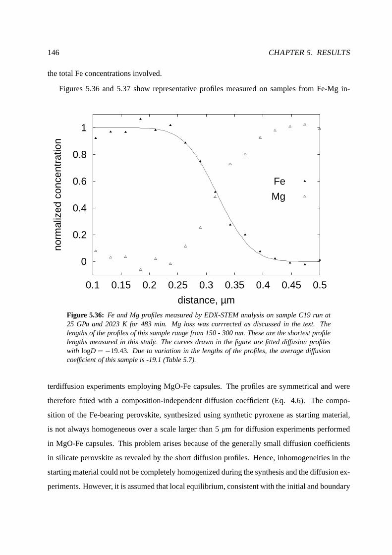
146 CHAPTER 5. RESULTS
the total Fe concentrations involved.
Figures 5.36 and 5.37 show representative profiles measuredon samples from Fe-Mg in-
0
0.2
0.4
0.6
0.8
1
0.1 0.15 0.2 0.25 0.3 0.35 0.4 0.45 0.5
norm
aliz
ed c
once
ntra
tion
distance, µm
Fe
Mg
Figure 5.36: Fe and Mg profiles measured by EDX-STEM analysis on sample C19run at25 GPa and 2023 K for 483 min. Mg loss was corrrected as discussed in the text. Thelengths of the profiles of this sample range from 150 - 300 nm. These are the shortest profilelengths measured in this study. The curves drawn in the figureare fitted diffusion profileswith logD = −19.43. Due to variation in the lengths of the profiles, the average diffusioncoefficient of this sample is -19.1 (Table 5.7).
terdiffusion experiments employing MgO-Fe capsules. The profiles are symmetrical and were
therefore fitted with a composition-independent diffusioncoefficient (Eq. 4.6). The compo-
sition of the Fe-bearing perovskite, synthesized using synthetic pyroxene as starting material,
is not always homogeneous over a scale larger than 5µm for diffusion experiments performed
in MgO-Fe capsules. This problem arises because of the generally small diffusion coefficients
in silicate perovskite as revealed by the short diffusion profiles. Hence, inhomogeneities in the
starting material could not be completely homogenized during the synthesis and the diffusion ex-
periments. However, it is assumed that local equilibrium, consistent with the initial and boundary
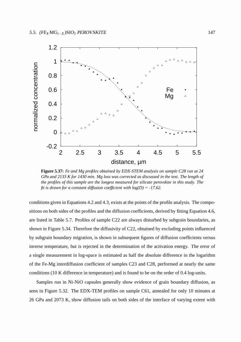
5.5. (FEXMG1−X)SIO3 PEROVSKITE 147
-0.2
0
0.2
0.4
0.6
0.8
1
1.2
2 2.5 3 3.5 4 4.5 5 5.5
norm
aliz
ed c
once
ntra
tion
distance, µm
FeMg
Figure 5.37: Fe and Mg profiles obtained by EDX-STEM analysis on sample C28run at 24GPa and 2133 K for 1430 min. Mg loss was corrected as discussedin the text. The length ofthe profiles of this sample are the longest measured for silicate perovskite in this study. Thefit is drawn for a constant diffusion coefficient with log(D) =-17.62.
conditions given in Equations 4.2 and 4.3, exists at the points of the profile analysis. The compo-
sitions on both sides of the profiles and the diffusion coefficients, derived by fitting Equation 4.6,
are listed in Table 5.7. Profiles of sample C22 are always disturbed by subgrain boundaries, as
shown in Figure 5.34. Therefore the diffusivity of C22, obtained by excluding points influenced
by subgrain boundary migration, is shown in subsequent figures of diffusion coefficients versus
inverse temperature, but is rejected in the determination of the activation energy. The error of
a single measurement in log-space is estimated as half the absolute difference in the logarithm
of the Fe-Mg interdiffusion coefficient of samples C23 and C28, performed at nearly the same
conditions (10 K difference in temperature) and is found to be on the order of 0.4 log-units.
Samples run in Ni-NiO capsules generally show evidence of grain boundary diffusion, as
seen in Figure 5.32. The EDX-TEM profiles on sample C61, annealed for only 10 minutes at
26 GPa and 2073 K, show diffusion tails on both sides of the interface of varying extent with

148 CHAPTER 5. RESULTS
Table 5.7: Results of the different perovskite diffusion experiments. XFeSiO3 is the compo-sition of the Fe-bearing endmember of the diffusion couple,for the Mg endmember no Fe ispresent at begin of the diffusion experiment, dur denotes duration, and unc is the uncertaintyof the Fe-Mg interdiffusion coefficient DFe−Mg in log-units.
Sample P, GPa T,K dur, min capsule XFeSiO3 DFe−Mg uncC13 24 2043 240 MgO-Fe 0.06 -18.8 0.4C19 24 2023 483 MgO-Fe 0.02-0.05 -19.1 0.4C22 24 2073 900 MgO-Fe 0.04 -18.21 0.4C23 24 2123 720 MgO-Fe 0.02-0.03 -18.4 0.4C28 24 2133 1430 MgO-Fe 0.06 -17.6 0.4C30 22 2273 373 MgO-Fe 0.05-0.07 -18.2 0.4C61 26 1800 10 Ni-NiO 0.10-0.12 n.d.3
C70 26 2173 60 Ni-NiO 0.09 -17.0 0.4C76 26 19732 570 Ni-NiO 0.11 -18.2 0.4
1 not included in calculations, as discussed in the text2 thermocouple break, temperature estimated from the heating power3 not determined, because no measurable profile developed (Fig. 5.38)
respect to distance (Fig. 5.38). This observation is interpreted as a grain boundary diffusion
component and its varying extent is due to the distance of thediffusion profile from the next
grain boundary. A sharp step in composition is observed at the center of the diffusion profile,
which is representative of the true bulk diffusion coefficient. Because diffusion coefficients of
silicate perovskite are very small (Table 5.7), virtually no diffusion profile due to bulk diffusion
developed during the annealing time of 10 minutes. Therefore, sample C61 can be regarded as a
zero time test.
Sample C76, performed at 26 GPa and 1973 K for 570 min, also shows tail contributions
but the profile due to bulk diffusion can be clearly resolved (Fig. 5.39). Most profile analyses
of sample C70 also show evidence of grain boundary diffusion. For this sample, the shortest
profile was regarded to represent the true lattice diffusioncoefficient. However, this still might
be an overestimation, because only one profile was taken intoaccount for deriving the diffusion
coefficient. Hence, it is not unequivocally demonstrated that this diffusivity does not include a
grain boundary diffusion contribution.
From this discussion, it becomes clear that in polycrystalline silicate perovskite diffusion
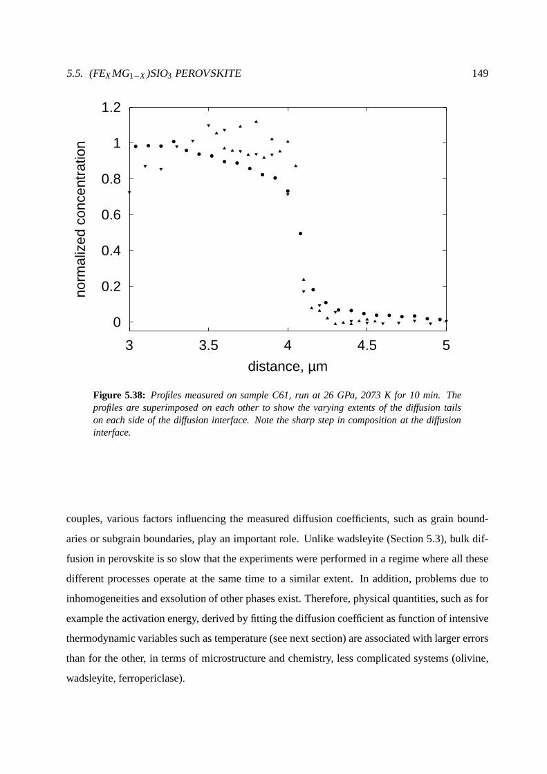
5.5. (FEXMG1−X)SIO3 PEROVSKITE 149
0
0.2
0.4
0.6
0.8
1
1.2
3 3.5 4 4.5 5
norm
aliz
ed c
once
ntra
tion
distance, µm
Figure 5.38: Profiles measured on sample C61, run at 26 GPa, 2073 K for 10 min. Theprofiles are superimposed on each other to show the varying extents of the diffusion tailson each side of the diffusion interface. Note the sharp step in composition at the diffusioninterface.
couples, various factors influencing the measured diffusion coefficients, such as grain bound-
aries or subgrain boundaries, play an important role. Unlike wadsleyite (Section 5.3), bulk dif-
fusion in perovskite is so slow that the experiments were performed in a regime where all these
different processes operate at the same time to a similar extent. In addition, problems due to
inhomogeneities and exsolution of other phases exist. Therefore, physical quantities, such as for
example the activation energy, derived by fitting the diffusion coefficient as function of intensive
thermodynamic variables such as temperature (see next section) are associated with larger errors
than for the other, in terms of microstructure and chemistry, less complicated systems (olivine,
wadsleyite, ferropericlase).

150 CHAPTER 5. RESULTS
0
0.2
0.4
0.6
0.8
1
1 1.5 2 2.5 3 3.5 4
Nor
mal
ized
con
cent
ratio
n
Distance, µm
C76, 1C76, 2C76, 3
Figure 5.39: Three different profiles measured on sample C76, annealed at26 GPa, 1973K for 570 minutes, superimposed onto each other. Note the consistency of the profile atintermediate concentrations and the tails on both sides of the interface. The dashed line is afit of Equation 4.6 with log(D) = -18.16.
5.5.5 Temperature dependence of Fe-Mg interdiffusion at 24GPa
Figure 5.40 shows Fe-Mg interdiffusion coefficients of (Mg,Fe)SiO3 perovskite as a function
of inverse temperature (Arrhenius diagram). Most of the experiments were performed at 24
GPa (Table 5.7). Only experiment C30 was at slightly lower pressure (22 GPa), employing an
18/8 assembly, whereas experiments employing Ni-NiO capsules were performed at 26 GPa in
order to stabilize the Fe-containing perovskite. As discussed in Section 5.5.1, the difference
in diffusivitiy due to the pressure effect should be negligible, much smaller than the analytical
error. Thus, no attempt was made to correct for the effect of pressure. All evidence presented in
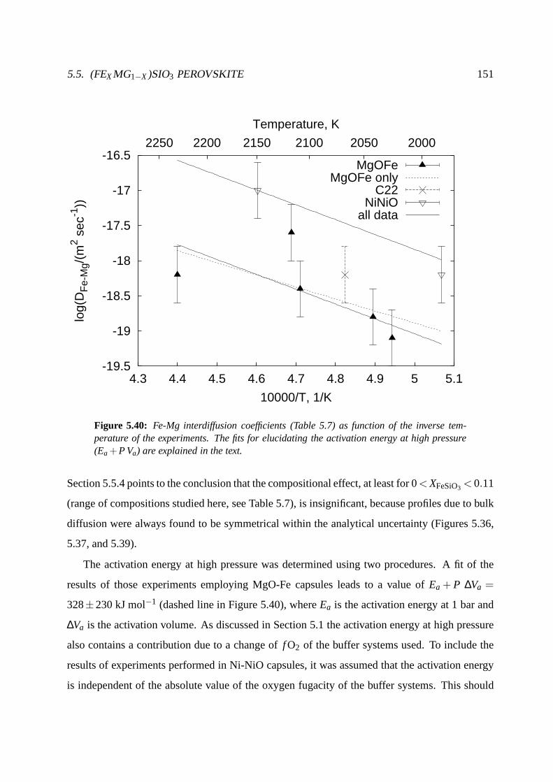
5.5. (FEXMG1−X)SIO3 PEROVSKITE 151
-19.5
-19
-18.5
-18
-17.5
-17
-16.5
4.3 4.4 4.5 4.6 4.7 4.8 4.9 5 5.1
2250 2200 21002150 2050 2000
log(
DF
e-M
g/(m
2 sec
-1))
10000/T, 1/K
Temperature, K
MgOFeMgOFe only
C22NiNiO
all data
Figure 5.40: Fe-Mg interdiffusion coefficients (Table 5.7) as function of the inverse tem-perature of the experiments. The fits for elucidating the activation energy at high pressure(Ea +P Va) are explained in the text.
Section 5.5.4 points to the conclusion that the compositional effect, at least for 0< XFeSiO3 < 0.11
(range of compositions studied here, see Table 5.7), is insignificant, because profiles due to bulk
diffusion were always found to be symmetrical within the analytical uncertainty (Figures 5.36,
5.37, and 5.39).
The activation energy at high pressure was determined usingtwo procedures. A fit of the
results of those experiments employing MgO-Fe capsules leads to a value ofEa + P ∆Va =
328±230 kJ mol−1 (dashed line in Figure 5.40), whereEa is the activation energy at 1 bar and
∆Va is the activation volume. As discussed in Section 5.1 the activation energy at high pressure
also contains a contribution due to a change off O2 of the buffer systems used. To include the
results of experiments performed in Ni-NiO capsules, it wasassumed that the activation energy
is independent of the absolute value of the oxygen fugacity of the buffer systems. This should

152 CHAPTER 5. RESULTS
be the case becausef O2 determines the abundance of point defects but not their energies of
formation or migration (see Equation 1.6 and Section 1.2.4). Hence, the diffusivities of C70
and C76 (Table 5.7, open triangles in Figure 5.40) were shifted systematically towards lower
diffusivity until the error of a linear fit of all data is simultaneously minimized. Determined by
this procedure, the overall activation energy at 24 GPa is 404±144 kJ mol−1 (for a shift of 1.2
log-units, solid lines in Figure 5.40). This value is valid for buffer systems with anf O2 variation
parallel to the Ni-NiO or Fe-FeO buffer, respectively. The shift of 1.2 log units corresponds to
an f O2 exponent of 1/3.3 if the absolute values off O2 differ by 4 log-units (Section 5.5.2). It
has to be emphasized that this value is subject to much uncertainty due to the extrapolation of the
f O2 values for the solid state buffers. Therefore, no attempt was made to interpret the oxygen
fugacity exponent in terms of point defects (see the derivation presented in Section 1.2.4).
The preferred model for Fe-Mg interdiffusion coefficientsDFe−Mg of (Mg,Fe)SiO3 per-
ovskite at 24 GPa and reducing conditions (∆ f O2 ≈−2.7, Table 5.6) is:
DFe−Mg = 3.3(1.2)×10−9 exp
(
−404000(144000)8.31441T(K)
)
m2
sec, (5.21)
and at an oxygen fugacity corresponding to the Ni-NiO buffer:
DFe−Mg = 5.1(2.0)×10−8 exp
(
−404000(144000)8.31441T(K)
)
m2
sec. (5.22)
The preexponential factor was derived by fixing the activation energy at 404 kJ mol−1. If DFe−Mg
has to be calculated at other oxygen fugacity conditions, af O21/3.3 correction might be employed
but it has to be kept in mind that this correction relies on theaccuracy of the extrapolations of the
oxygen fugacities of the Ni-NiO and Fe-FeO buffers, which are poorly constrained at present.
Equations 5.21 and 5.22 do not take any directional dependence into account because from
a structural point of view the directional dependence should be relatively weak (Section 1.3.1).
However, some of the scatter observed in Figure 5.40 might arise from variations in crystallo-
graphic orientation.
At 1973 K and 24 GPa, for oxygen fugacities close to the Ni-NiObuffer, the Fe-Mg in-
terdiffusion coefficient of (Mg,Fe)SiO3 perovskiteDpvskFe−Mg is 1.0×10⁻¹⁸ m2 sec−1 (Equation
5.22). At the same conditions the Fe-Mg interdiffusion coefficient for ferropericlaseD f pFe−Mg
is 2.1×10⁻¹⁴ m2 sec−1 for XFeO= 0.05 (Equation 5.14). Hence, the ratioD f pFe−Mg/Dpvsk
Fe−Mg is

5.5. (FEXMG1−X)SIO3 PEROVSKITE 153
2× 10⁴, nearly the same value that was estimated in Section 5.5.2. The silicon self-diffusion
coefficient of silicate perovskite at 1973 K and 24 GPa is 3.5×10⁻¹⁹ m2 sec−1 using data of
Yamazaki et al. (2000). Hence, silicon self-diffusion at these conditions is only approximately
a factor of 3 slower than Fe-Mg interdiffusion estimated employing Equation 5.22. If the Si
self-diffusion coefficient is compared to Fe-Mg interdiffusion at reducing conditions (Equation
5.21, 6.7×10⁻²⁰ m2 sec−1) it is found that Si self-diffusion is faster than Fe-Mg interdiffusion.
This has important implications for the rheology of the lower mantle which in a diffusional creep
regime is determined by the slowest diffusing species. At reducing conditions the slowest dif-
fusing species might be diffusion of the divalent cations rather than Si diffusion. This situation
is totally different from relative diffusion rates at conditions of the upper mantle, because for
minerals such as olivine, Si diffusion is much slower than Fe-Mg interdiffusion (Bejina, 1999).
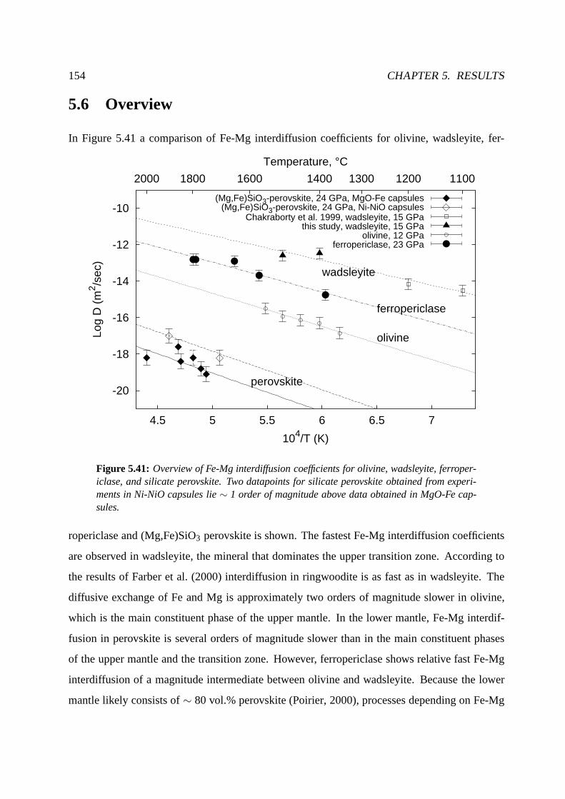
154 CHAPTER 5. RESULTS
5.6 Overview
In Figure 5.41 a comparison of Fe-Mg interdiffusion coefficients for olivine, wadsleyite, fer-
-20
-18
-16
-14
-12
-10
4.5 5 5.5 6 6.5 7
1400 110012001300160018002000
Log
D (
m2 /s
ec)
104/T (K)
Temperature, °C
wadsleyite
olivine
perovskite
ferropericlase
(Mg,Fe)SiO3-perovskite, 24 GPa, MgO-Fe capsules(Mg,Fe)SiO3-perovskite, 24 GPa, Ni-NiO capsules
Chakraborty et al. 1999, wadsleyite, 15 GPathis study, wadsleyite, 15 GPa
olivine, 12 GPaferropericlase, 23 GPa
Figure 5.41: Overview of Fe-Mg interdiffusion coefficients for olivine,wadsleyite, ferroper-iclase, and silicate perovskite. Two datapoints for silicate perovskite obtained from experi-ments in Ni-NiO capsules lie∼ 1 order of magnitude above data obtained in MgO-Fe cap-sules.
ropericlase and (Mg,Fe)SiO3 perovskite is shown. The fastest Fe-Mg interdiffusion coefficients
are observed in wadsleyite, the mineral that dominates the upper transition zone. According to
the results of Farber et al. (2000) interdiffusion in ringwoodite is as fast as in wadsleyite. The
diffusive exchange of Fe and Mg is approximately two orders of magnitude slower in olivine,
which is the main constituent phase of the upper mantle. In the lower mantle, Fe-Mg interdif-
fusion in perovskite is several orders of magnitude slower than in the main constituent phases
of the upper mantle and the transition zone. However, ferropericlase shows relative fast Fe-Mg
interdiffusion of a magnitude intermediate between olivine and wadsleyite. Because the lower
mantle likely consists of∼ 80 vol.% perovskite (Poirier, 2000), processes depending on Fe-Mg
5.7. EXPERIMENTAL COMPLICATIONS 155
interdiffusion should be governed by very slow diffusivities (see further discussion in Section
6.5.2).
5.7 Diffusion experiments at high pressure: Experimentalcomplications
5.7.1 High pressure versus low pressure experiments
At 1 bar, diffusion experiments are performed in furnaces that have a comparatively large hot
spot region. Hence, at the position of the diffusion couple no significant temperature gradients
are observed. In high pressure sample assemblies (Sections2.2 and 2.5), the region of the hot
spot is significantly smaller, potentially leading to significant thermal gradients. Knowing the
diffusivities of the minerals investigated in this study (Sections 5.2 - 5.5), enables the effect of
thermal gradients to be investigated by numerical simulations (Section 5.7.2). Another point of
interest (at 1 bar and at high temperature) is the contribution of diffusion during initial heating
of the experiments, especially if absolute diffusivities are relatively large and experimental du-
rations short. As with temperature gradients, if diffusioncoefficients are known, the role of the
heating effect can be further investigated by numerical simulations (Section 5.7.3).
5.7.2 Temperature gradients
Temperature gradients in the 10/4 assembly can be as large as100 K mm−1 (Trønnes and Frost,
2002). The longest profiles investigated in this study were observed for ferropericlase (Section
5.4), with a profile length of 100-200µm. Therefore, Fe-Mg interdiffusion profiles in ferroperi-
clase are most likely to have been affected by thermal gradients across the diffusion zone. With
a temperature gradient of 100 K mm−1 and a profile length of around 100-200µm, the temper-
ature variation along the diffusion profile is on the order of10-20 K. Numerical simulations by
finite differences using Equation 5.13, but allowing the temperature to vary linearly along the
profile, were performed for the range of diffusivities obtained in this study. The temperature of
the experimentTexpwas taken to be representative for the original interface ofthe diffusion pro-
file. At the hotter end of the profile of the simulation, the temperature can then be expressed as
Tl = Texp+grad 1/2 lx, wheregrad is the temperature gradient andlx is the length of the profile

156 CHAPTER 5. RESULTS
simulation. For the simulation, Equation 5.13 is inserted in Equation 1.2:
∂C∂t
=∂∂x
(
D0 ·exp
(
−EA−A ·XFeO+(P−Pre f ) ·∆VA
R· (Tl −grad x)
)
∂C∂x
)
(5.23)
Figure 5.42 illustrates the simulation at the conditions ofexperiment C48 (Table 5.5), which re-
sulted in the longest profile observed in a 10/4 assembly in this study. The simulations employing
0.36
0.3615
50 60 70 80 90 100 110 120
XF
eO
48 µm
3 µm
no gradient100 K/mm
1000 K/mm
2020
2040
2060
2080
2100
2120
50 100 150 200 250 3000
0.1
0.2
0.3
0.4
0.5
Tem
pera
ture
, K
XF
eODistance, µm
Texp
temperatureStarting concentrationXFeO, dt/dx = 0 K/mm
XFeO, dT/dx = 100 K/mmXFeO, dT/dx = 1000 K/mm
Figure 5.42: Effect of thermal gradients in the 10/4 assembly. The temperature varies lin-early along the profile (left y axis, shown for a temperature gradient dT /dx of 100 K/mm).The simulations (right y axis) are shown for dT /dx = 0, 100, and 1000 K/mm. The insetshows a blow up of the profiles in the region of 50-120 µm to showthe extent of maximumprofile lengthening.
Equation 5.23 show that effects of profile lengthening or shortening are negligible (∼ 3 µm at the
hot end and≪ 1 µm at the cold end of the profiles) for a thermal gradient of 100 K/mm. The dif-
fusion coefficient atXFeO= 0.3, due to the thermal gradient, is∼ 2.8 % larger. This deviation is a
factor of 10 smaller than the experimental error of∼ 30 % (0.3 log-units, Section 5.4.3). Hence,
even for temperature gradients of 100 K/mm and a profile length of∼ 200µm, the results would
not be significantly affected. For temperature gradients much larger than 100 K/mm, the error
5.7. EXPERIMENTAL COMPLICATIONS 157
would become significant, for example approximately 30% at the profile ends for 1000 K/mm
with a displacement of the profile of∼ 48µm at the hotter end (Figure 5.42).
Aside from pure distortion due to a change of diffusivity, temperature gradients can poten-
tially also lead to Soret diffusion. For ferropericlase, this effect would be different in the two
assembly types used in this study because temperature gradients in the 14/8 cell are much smaller
in comparison to the 10/4 cell. Therefore a kink or discontinuity would appear in the pressure
correlation if the Soret effect leads to a significant contribution of the diffusional flux. Such a
kink is not observed however (Figs. 5.28, 5.29), so significant Soret diffusion can be excluded.
5.7.3 Heating effects
Some diffusion inevitably occurs while the sample is being heated. However, at 1873 K and 8
GPa, results of the time series shown in Fig. 5.27 indicate that this has little or no effect on the
derived diffusion coefficients at these conditions. The contribution to the diffusion profiles during
heating at all conditions was simulated by finite differences using Eq. 5.13. In an initial heating
phase the temperature was varied from room temperature to the final temperature using the actual
heating rates of the experiments. In practice this is achieved by approximating the heating with a
step like temperature profile. At each step, normally with a stepsize of 1 K, diffusion is simulated
and the resulting profile is taken as the initial distribution for the next temperature step. If the
experimental temperatureTexp is reached, the calculations are continued in the same way asin
all other profile simulations. Figure 5.43 shows an example of the ferropericlase system, taking
a heating rate of 3.5 K/sec which is slightly smaller that theactual heating rate of 5 K/sec (worst
case scenario).
The simulations show that diffusion profiles with lengths ofseveral microns, depending on
the heating rate and mineral system, develop during initialheating (∼ 25 µm for the example
in Figure 5.43). The difference between simulations employing these extended profiles as the
initial condition and simulations using an ideal step function as the initial condition vanishes
very quickly, however, with progressive diffusion. After less than 5 minutes no significant differ-
ences can be observed for the combinations of heating rate and high temperature annealing times
used in this study. For C55, even for a longer heating time than the real heating time (Figure

158 CHAPTER 5. RESULTS
0.346
0.348
0.35
0.352
0.354
550 555 560 565 570
0.8 µm
0.05
0.1
0.15
0.2
0.25
0.3
0.35
0.4
460 480 500 520 540 560 580 600
XF
eO
dimensions, µm
ideal3.5 K/sec
heat + annealideal anneal
Figure 5.43: Effect of diffusion occuring during initial heating of experiment C55 (Table5.5). The dashed line shows an ideal step function as initialcondition (Eq. 4.2). Theblack dots show the profile that developes in the simulation solely due to the heating effectwith a heating rate of 3.5 K/sec, slightly smaller than the actual heating rate of 5 K/sec. Thediamonds represent the profile taking the heating effect into account and are compared to theprofile simulated without heating effect (solid line). The deviation between the two profilesafter 21 minutes (experimental duration) is on the order of 0.8 µm only.
5.43), the deviation of absolute diffusivities is smaller than 3 %, corresponding to better than
0.02 log-units (with an experimental error of 0.3 log-units). Experiments employing diffusion
couples of olivine, wadsleyite and silicate perovskite were performed always with a larger ratio
of experimental duration at high temperature to heating time. Hence, the effect of heating is
even smaller for these minerals as compared to ferropericlase. Therefore the profiles observed in
this work only contain information about the diffusional properties at high temperature and it is
mathematically justified to use an ideal step function as theinitial condition in the simulation of
the profiles.

Chapter 6
Discussion
6.1 Introduction
The results obtained in this study can be used to calculate Fe-Mg interdiffusion coefficients at
the oxygen fugacity of the Ni-NiO buffer for olivine in the upper mantle, wadsleyite in the tran-
sition zone and ferropericlase and silicate perovskite in the uppermost part of the lower mantle.
The temperature and pressure conditions of the experimentsdirectly correspond to the condi-
tions prevailing in the mantle to a depth of 700 km. For constraining diffusivities and a better
understanding of kinetics in the lower mantle, results for ferropericlase (Section 5.4) and sili-
cate perovskite (Section 5.5) are extrapolated over the entire pressure and temperature range of
the lower mantle in Section 6.2 using ab initio calculationsto constrain the activation volume at
pressures> 25 GPa (Ita and Cohen, 1997; Wright and Price, 1993). Taking an adiabatic model
of temperature and the Preliminary Reference Earth Model (PREM, Dziewonski and Anderson,
1981) for the pressure variation with depth into account, diffusion coefficients, characteristic for
the depth range of 0 to 700 km, are calculated in Section 6.3 together with estimates for the
lower mantle. The slow Fe-Mg interdiffusion rates of silicate perovskite exert strong limitations
on the experimental investigation of multiphase element partitioning involving this mineral. This
problem is further discussed in Section 6.4.
The following sections highlight selected geological applications of the diffusion coefficients
determined in this study. Olivine and wadsleyite Fe-Mg interdiffusion coefficients are used in
Section 6.5.1 to constrain the kinetics of the olivine-wadsleyite phase boundary in the Earth’s
mantle. Because the lower mantle consists mainly of ferropericlase and perovskite, the diffu-
159

160 CHAPTER 6. DISCUSSION
sional properties of a minor phase (ferropericlase) embedded in a matrix with a much smaller
diffusion coefficient (perovskite) is investigated in Section 6.5.2. These results are then used
to constrain the lifetime of heterogeneities of varying sizes in the lower mantle (Section 6.5.3)
and the possible extent of interaction at the core-mantle boundary during Earth’s history (Section
6.5.4). The final section (Section 6.5.5) gives an estimate of the extent of possible reequilibration
in the lower mantle during core formation following an earlymagma ocean stage.
6.2 Extrapolations towards lower mantle conditions
6.2.1 Ferropericlase
In order to calculate Fe-Mg interdiffusion coefficients of ferropericlase over the entire pressure-
temperature range of the lower mantle, the results of this study are combined with results of ab
initio calculations on how the activation volume evolves asa function of pressure up to the pres-
sure at the core-mantle boundary, which is approximately 136 GPa (Dziewonski and Anderson,
1981).
Theoretical considerations predict that the activation volume should decrease with increasing
pressure (Karato, 1981; Poirier and Liebermann, 1984; Mills et al., 1991). Ita and Cohen (1997)
calculated free energies for vacancy pair formation and migration of Mg and O in pure MgO at
pressures from 0 to 140 GPa and temperatures from 1000 to 5000K. Using these data together
with calculated lattice parameters enabled these authors to calculate the decrease in the activation
volume of the intrinsic Mg self-diffusion coefficient with increasing pressure. However, experi-
mental and theoretical evidence shows that Mg diffusion in MgO occurs by an extrinsic diffusion
mechanism at all experimental conditions so far investigated (Sempolinski and Kingery, 1980;
Wuensch, 1983; Vocadlo et al., 1995; Van Orman et al., 2003). This is also likely to be the case
for the Fe-Mg interdiffusion experiments reported in this study. Hence, to compare the results
of Ita and Cohen (1997) with experimental results only the migration volumeVm = ∂Gm/∂P,
whereGm is the free energy of migration of the diffusion mechanism, has to be used. The acti-
vation volume of 3.0 cm3 mol−1 for Mg tracer diffusion determined by Van Orman et al. (2003)
agrees well with the migration volume of 3.1 cm3 mol−1 calculated employing free energies of
migration by Ita and Cohen (1997) between 0 and 20 GPa at 2000 K. It will be assumed here

6.2. EXTRAPOLATIONS TOWARDS LOWER MANTLE CONDITIONS 161
that the data for the free energy of migration reported in Itaand Cohen (1997) can also be used
to constrain the pressure dependence of the activation volume of (FexMg1−x)O ferropericlase at
pressures greater than 23 GPa.
The migration entropySm calculated asSm = ∂Gm/∂T from the values of Ita and Cohen
(1997) is approximately constant between 0 and 140 GPa indicating that the preexponential factor
is pressure independent. In this case the activation volume∆Va(P) at any pressure P and constant
temperature is given by (Poirier, 2000):
∆Va(P) = −RT∂ lnD(P)
∂P=
∂∆Ha(P)
∂P, (6.1)
whereD(P) is the diffusion coefficient at pressure P and∆Ha(P) is the activation enthalpy at
pressureP. As an approximation, the average activation volume between 1 bar and pressureP
was estimated from:
∆Vavga (P) =
∆Ha(P)−∆Ha(1 bar)P−1 bar
. (6.2)
Values for the activation enthalpy∆Ha(T,P) at temperatureT and pressureP can be calculated
employing the results of Ita and Cohen (1997) from∆Ha(T,P) = ∆Gm(T,P)+T ·∆Sm(P), where
∆Gm(T,P) is the migration free energy at temperatureT and pressureP and∆Sm(P) is the migra-
tion free entropy at pressureP. Between 0 and 140 GPa at 3000 K an average migration volume
of 1.35 cm3 mol−1 was derived in this way for extrinsic Mg self-diffusion. Assuming a similar
pressure effect on the activation volume for Fe-Mg interdiffusion leads to an average activation
volume of 1.4 cm3 mol−1 for calculation of diffusivities at the core mantle boundary.
The average activation volume between 0 and 140 GPa of 1.4 cm3 mol−1 together with the
experimentally determined value between 0 and 23 GPa of 3.3 cm3 mol−1 (Section 5.4) can be
used to constrain the pressure dependence of the activationvolume of Fe-Mg interdiffusion in
ferropericlase making a linear approximation:
∆Va = ∆V0a +P×∆V ′
a. (6.3)
The value for the zero pressure activation volume∆V0a is 0.367 J bar−1 and the pressure derivative
∆V ′a becomes−1.624×10⁻⁷ J bar−2.

162 CHAPTER 6. DISCUSSION
6.2.2 Silicate perovskite
Extrapolation of perovskite diffusion data to pressures inexcess of 26 GPa is less well con-
strained than for ferrropericlase because the activation volume of diffusion in silicate perovskite
could not be determined by the experimental results of this study. This is due to the very re-
stricted pressure range within the silicate perovskite stability field that can be generated by the
multianvil apparatus employing sintered WC cubes. In addition, questions concerning the struc-
tural stability of this phase still remain unsolved (Section 1.3.1). Therefore, in the following
sections two models of the activation volume of Fe-Mg interdiffusion in (Mg,Fe)SiO3 perovskite
are considered:
• The magnitude of the activation volume is considered to be zero. Thus, the activation
energy determined at 24 GPa (404 kJ mol−1, Equation 5.21 and 5.22) is valid over the
entire pressure and temperature range of the lower mantle along the Ni-NiO buffer.
• The activation volume is 2.1 cm3 mol−1, based on the value determined in a theoretical
study of Mg self-diffusion in pure MgSiO3 by Wright and Price (1993). In this approach it
is assumed that, as for ferropericlase (see Section 6.2.1),the activation volume for diffusion
of Mg in MgSiO3 is also directly applicable to Fe-Mg interdiffusion in (Mg,Fe)SiO3.

6.3. FE-MG INTERDIFFUSION ALONG A PRESENT DAY GEOTHERM 163
6.3 Fe-Mg interdiffusion along a present day geotherm
In Figure 6.1 diffusion coefficients along an adiabat for an average mantle below mid-ocean
ridges (Herzberg and Zhang, 1996) are calculated below the base of the lithosphere, i.e. at pres-
sures in excess of 3 GPa (depth> 96 km). For all minerals, results corresponding to the Ni-NiO
buffer were used. The steps in temperature occurring at the phase transition boundaries are due to
the heat of transformation. Depending on the mode of convection, these temperature steps would
relax around the transition depth but the steps in diffusivity observed at the phase transition points
would still be preserved. It should be emphasized that for olivine, above 3 GPa, the diffusivity
decreases due to the effect of pressure on diffusion even though the temperature increases from∼1700 K to 1850 K. At 13.5 GPa theα-β phase boundary is reached. The diffusion coefficient for
olivine at this pressure and a temperature of 1850 K isDFe−Mg = (5.9±0.2)×10−16 m2 sec−1 at
the Ni-NiO buffer andXFe2SiO4 = 0.1. This value is a factor of∼ 150 smaller than the value at 1
bar at the same temperature, composition and relative oxygen fugacity (Ni-NiO buffer). Hence,
pressure effect has a large influence on the Fe-Mg interdiffusion coefficient at high pressure that
was not taken into account in former studies (for example Solomatov and Stevenson, 1994).
For the high pressure polymorphs of olivine, wadsleyite andringwoodite, the activation vol-
ume of 6.1 cm3 mol−1 of Farber et al. (2000) was used in combination with Equation5.12. It
is assumed that Fe-Mg interdiffusion is equally fast in bothhigh-pressure polymorphs of olivine
(Chakraborty et al., 1999; Farber et al., 2000). As shown in Section 5.3.5 and Figure 5.22 a
jump in the Fe-Mg interdiffusion coefficient by∼ 3.5 orders of magnitude occurs at the 410
km discontinuity. If the activation volume of 6.1 cm3 mol−1 predicted by Farber et al. (2000)
is correct, the effect of pressure on diffusion along the adiabat results in Fe-Mg interdiffusion
coefficients for wadsleyite and ringwoodite which, at the 670 km discontinuity (∼ 23 GPa), are
relatively similar to the values derived for ferropericlase. On the contrary, Fe-Mg interdiffusion
in silicate perovskite is orders of magnitude slower (approximately by a factor of 2×10⁴, see
Section 5.5.5). An increase in diffusivity for silicate perovskite with increasing pressure along
the adiabat shown in Figure 6.1 is observed because a possible effect of pressure (Va 6= 0) was
not taken into account in deriving the values for silicate perovskite shown in Figure 6.1 (compare
with Equation 5.22). Depending on the oxidation state of thelower mantle, which is probably

164 CHAPTER 6. DISCUSSION
-19
-18
-17
-16
-15
-14
-13
-12
-11
-10
5 10 15 20 25 301700
1750
1800
1850
1900
1950
2000
2050
2100400 670150
Log(
D/(
m2 s
ec-1
)
tem
pera
ture
, K
Pressure, GPa
Depth, km
ol
wds/rgw
pvsk
fpadiabat
Figure 6.1: Fe-Mg interdiffusion coefficients for different minerals in the upper mantle, thetransition zone and the top of the lower mantle. All diffusion coefficients are given for anoxygen fugacity close to the Ni-NiO buffer, and an Fe component mole fraction of 0.1. Theadiabat (right y axis) is from Figure 20 of Herzberg and Zhang(1996) and is representativeof a present day average mantle beneath oceanic ridges. Olivine diffusion coefficients, givenas log(D) on the left y axis, were calculated using Equation 5.11, and applying a correctionfactor of 1.6 to account for the compositional effect (see Section 5.2.3). Ringwoodite isconsidered to have the same diffusion properties as wadsleyite (Farber et al., 2000). InEquation 5.12 an activation volume of 6.1 cm3 mol−1 (Farber et al., 2000) was used. Forferropericlase and silicate perovskite, Equations 5.14 and 5.22 were used, respectively.
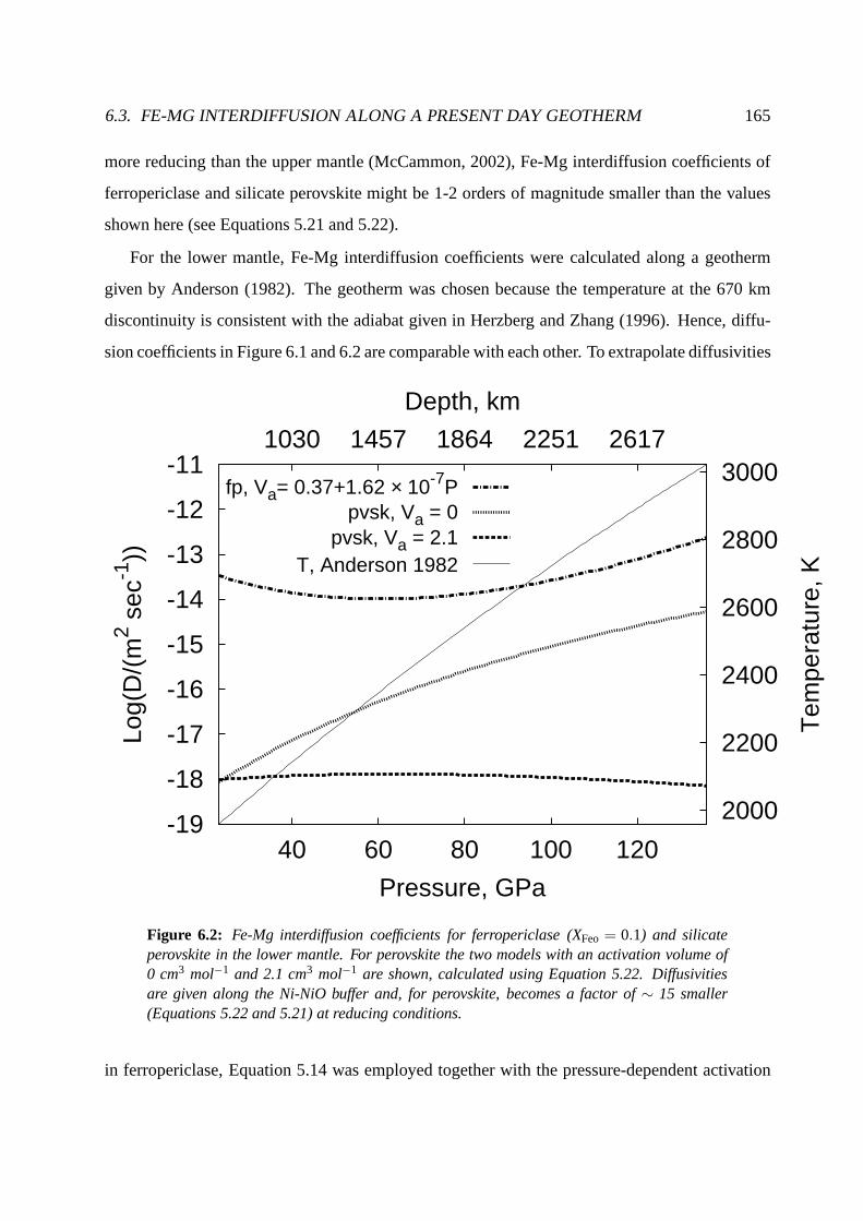
6.3. FE-MG INTERDIFFUSION ALONG A PRESENT DAY GEOTHERM 165
more reducing than the upper mantle (McCammon, 2002), Fe-Mginterdiffusion coefficients of
ferropericlase and silicate perovskite might be 1-2 ordersof magnitude smaller than the values
shown here (see Equations 5.21 and 5.22).
For the lower mantle, Fe-Mg interdiffusion coefficients were calculated along a geotherm
given by Anderson (1982). The geotherm was chosen because the temperature at the 670 km
discontinuity is consistent with the adiabat given in Herzberg and Zhang (1996). Hence, diffu-
sion coefficients in Figure 6.1 and 6.2 are comparable with each other. To extrapolate diffusivities
-19
-18
-17
-16
-15
-14
-13
-12
-11
40 60 80 100 120
2000
2200
2400
2600
2800
30001030 1457 1864 2251 2617
Log(
D/(
m2 s
ec-1
))
Tem
pera
ture
, K
Pressure, GPa
Depth, km
fp, Va= 0.37+1.62 × 10⁻⁷Ppvsk, Va = 0
pvsk, Va = 2.1T, Anderson 1982
Figure 6.2: Fe-Mg interdiffusion coefficients for ferropericlase (XFeo = 0.1) and silicateperovskite in the lower mantle. For perovskite the two models with an activation volume of0 cm3 mol−1 and 2.1 cm3 mol−1 are shown, calculated using Equation 5.22. Diffusivitiesare given along the Ni-NiO buffer and, for perovskite, becomes a factor of∼ 15 smaller(Equations 5.22 and 5.21) at reducing conditions.
in ferropericlase, Equation 5.14 was employed together with the pressure-dependent activation

166 CHAPTER 6. DISCUSSION
volume estimated in Equation 6.3. The calculated diffusioncoefficients (Figure 6.2) show that in
the upper part of the lower mantle the Fe-Mg interdiffusion coefficient would decrease slightly
due to the pressure effect whereas in the lower part of the lower mantle the activation volume
becomes essentially zero and diffusivities become faster due to the temperature effect. How-
ever, the Fe-Mg diffusion coefficient does not vary by more than a factor of 10. Therefore, a
diffusion coefficient of 4×10⁻¹⁴ m2 sec−1 atXFeO= 0.1 is a good estimate for the Fe-Mg inter-
diffusion coefficient of ferropericlase in the lower mantlealong the Ni-NiO buffer and is almost
independent of depth.
For silicate perovskite the two end-member models for the effect of pressure (Section
6.2.2) lead to a steady increase in diffusivities in the casewhere the activation volume∆Va =
0 cm3 mol−1 (from ∼ 10−18 m2 sec−1 at 24 GPa to 5×10⁻¹⁵ m2 sec−1 at 136 GPa), whereas
diffusivities are essentially constant, approximately 10−18 m2 sec−1, with ∆Va = 2.1 cm3 mol−1
(Wright and Price, 1993). These values are for oxygen fugacity conditions close to the Ni-
NiO buffer. In the case of more reducing conditions (equivalent to f O2 prevailing inside the
MgO-Fe capsules) the Fe-Mg interdiffusion coefficients area factor of 14 smaller (see Equa-
tions 5.21 and 5.22) leading to an effective diffusion coefficient of 7×10⁻²⁰ m2 sec−1 in the
case of∆Va = 2.1 cm3 mol−1. In both models of the activation volume (∆Va = 0 cm3 mol−1
or ∆Va = 2.1 cm3 mol−1), diffusivities in perovskite are always smaller than in ferropericlase,
implying that silicate perovskite equilibration lengths are also smaller and equilibration times are
longer compared to ferropericlase. Because the lower mantle is believed to be essentially a two-
phase mixture of silicate perovskite and ferropericlase, the diffusional properties of a two-phase
aggregate consisting of ferropericlase inclusions in a perovskite matrix is further discussed in
Section 6.5.2.

6.4. TIME SCALES OF FE-MG PARTITIONING EXPERIMENTS 167
6.4 Time scales of Fe-Mg partitioning experiments involvingsilicate perovskite
For different time scales, the characteristic diffusion lengthxdi f f can be calculated by (Section
4.2):
xdi f f = k×√
D t, (6.4)
wherek is a proportionality factor as discussed in Section 4.2. Theproportionality factork
depends on the nature of the diffusion problem and is estimated to be 6.6 in the case of two
semi-infinite media (Figure 4.2) and 3.3 in the case of diffusion into a half-space.
The very small Fe-Mg interdiffusion coefficients of silicate perovskite, especially at reducing
conditions, impose severe limits on the feasability of Fe-Mg equilibrium partitioning experi-
ments. In Frost and Langenhorst (2002), it was not possible to achieve equilibrium in experi-
ments employing Fe-capsules. Equation 5.21 gives an equilibration distance of∼ 400 nm at 24
GPa and 1923 K for 24 hours at reducing conditions, comparable to the conditions of the exper-
iments of Frost and Langenhorst (2002). Clearly, grains with a diameter of several microns can
not fully equilibrate at such low oxygen fugacities. At moreoxidizing conditions, Equation 5.22
predicts equilibration distances of 0.8-1.3 microns (for times of 8 - 20 h at 1923 K and 24 GPa),
which are only slightly smaller than the grain size of 1-2µm observed for Al2O3-free perovskite
by Frost and Langenhorst (2002).
It is also possible to estimate the time of reequilibration by using a solution for spherical
particles (Equations 6.18, 6.19 and 6.21 in Crank, 1979). Atreducing conditions (Equation 5.21)
the time needed to equilibrate the center of a spherical grain with a diameter of 1 micron to
50% takes more than 10 days whereas for oxidizing conditions(Ni-NiO buffer, Equation 5.22)
the same amount of equilibration is reached in 18 h and therefore within the experimental time
frame. In addition, Frost and Langenhorst (2002) used Re capsules, where the oxygen fugacity is
supposed to be even higher than in the Ni-NiO capsules used inthis study. This is shown by the
fact that one experiment of Frost and Langenhorst (2002) employing a Re-ReO2 capsule showed
exactly the same results for the partitioning data comparedwith the unbuffered Re capsules. In
addition, the diffusion experiments performed by Yamazakiand Irifune (2003) using ferroperi-
clase diffusion couples in Re capsules are consistent with very oxidizing conditions at pressures
168 CHAPTER 6. DISCUSSION
of 23-26 GPa (but see the disscussion in Section 5.4.7). Hence, microprobe analyses should be
relatively close to the true equilibrium concentrations for experiments at oxidizing conditions.
For more reducing conditions and the same pressure and temperature conditions as used by Frost
and Langenhorst (2002) equilibration times should be at least on the order of a few weeks in
order to result in an equilibrium distribution. Other phases like ferropericlase or ringwoodite
equilibrate within at least 2 orders of magnitude shorter times because diffusion coefficients are
more than 4 orders of magnitude faster (Section 5.6).
6.5. APPLICATIONS TO GEOLOGICAL PROBLEMS 169
6.5 Applications to geological problems
6.5.1 Kinetics of the olivine-wadsleyite phase boundary
As described in Rubie et al. (1993), the kinetics of the high-pressure phase transformation of
olivine to wadsleyite are controlled by diffusion if nucleation occurs close to equilibrium. The
growth rate should follow a parabolic rate law according to:
x =
√
DFe−Mg
t, (6.5)
whereDFe−Mg is the Fe-Mg interdiffusion coefficient. Equation 6.5 is only valid as long as the
diffusion halos of the matrix do not impinge on each other.
Figure 6.3 shows the physical model used in this study to constrain the kinetics of the phase
transition in order to investigate a possible oversteppingof the equilibrium phase boundaries
which could lead in response to convective flow across the 410km disontinuity to a broadening
or narrowing of the transition. It is assumed that wadsleyite during convective descent and olivine
during convective ascent nucleate heterogenously on grainboundaries. Therefore, the distance
over which diffusion has to occur is the grain diameter whichis assumed to be 1 cm. A first
estimate if the phase transition occurs close to equilibrium can be made by considering how
long it takes to adapt to a new Fe-Mg equilibrium distribution along the P-T path inside the
transformation boundaries by:
t =x2
k2√
DFe−Mg, (6.6)
where k is the proportionality factor of Equation 6.4. As shown later in Section 6.5.3 the pro-
portionality factork is on the order of 1.6 for the equilibration of a spherical grain. Using the
results obtained by Akaogi et al. (1989), the temperature across the phase transition for a mantle
geotherm varies between 1695 - 1742 K at pressures between 13.3 and 14 GPa. Therefore, the
time to equilibrate a grain of wadsleyite with a diameter of 1cm is on the order of 3−5×10⁷sec
depending on composition, temperature and pressure, whereas for olivine∼ 1.5×10¹¹ sec are
needed as shown in Table 6.1. Considering a convection velocity uc of 5 cm year−1, Table
6.1 shows that after convecting a distancex = uc t of 50-80 cm wadsleyite grains have already
reequilibrated, whereas for olivine this characteristic distance is on the order of 240 m.

170 CHAPTER 6. DISCUSSION
13.3
14
1695 1742
13.3
14
Pre
ssur
e, G
Pa
Temperature, K
Wds + Ol
Ol
Wds
XOl = 0.10XWds = 0.19
XWds = 0.10XOl = 0.05
T-Profile
Figure 6.3: Physical model of the olivine-wadsleyite phase transitionusing results obtainedin Akaogi et al. (1989). The dashed line is a temperature profile (T profile) in the normalmantle taken from Figure 10 in Akaogi et al. (1989) together with the phase boundaries.Also given are XFe2SiO4 of olivine and wadsleyite (Xol, Xwds) coexisting in equilibrium at thephase boundaries. At intermediate points along the temperature profile the concentrationsof wadsleyite and olivine change systemtically between these values. The bulk Fe content isassumed to be XFe2SiO4 = 0.1.
Clearly, the rate of diffusion in wadsleyite is always fast enough to reequilibrate to the new
equilibrium concentration inside the transformation region. In order to see if the distance of
240 m, derived in Table 6.1 for olivine, can lead to a non-equilibrium distribution and hence
to a metastable overstep of the phase boundaries, the evolution of concentration in wadsleyite
and olivine during convection is modelled by finite difference simulations with a moving phase
boundary. The moving boundary results from the difference in flux across the interface between
growing wadsleyite and an olivine matrix or vice versa during progressive change of the equilib-
rium concentrations of coexisting olivine and wadsleyite within the transformation field leading
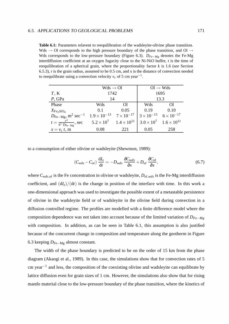
6.5. APPLICATIONS TO GEOLOGICAL PROBLEMS 171
Table 6.1: Parameters relavent to reequilibration of the wadsleyite-olivine phase transition.Wds→ Ol corresponds to the high pressure boundary of the phase transition, and Ol→Wds corresponds to the low-pressure boundary (Figure 6.3).DFe−Mg denotes the Fe-Mginterdiffusion coefficient at an oxygen fugacity close to the Ni-NiO buffer, t is the time ofreequilibration of a spherical grain, where the proportionality factor k is 1.6 (see Section6.5.3), r is the grain radius, assumed to be 0.5 cm, and x is thedistance of convection neededto reequilibrate using a convection velocityvc of 5 cm year−1.
Wds→ Ol Ol → WdsT, K 1742 1695P, GPa 14 13.3Phase Wds Ol Wds OlXFe2SiO4 0.1 0.05 0.19 0.10DFe−Mg, m2 sec−1 1.9×10⁻¹³ 7×10⁻¹⁷ 3×10⁻¹³ 6×10⁻¹⁷
t = r2
k2 DFe−Mg, sec 5.2×10⁷ 1.4×10¹¹ 3.0×10⁷ 1.6×10¹¹
x = vc t, m 0.08 221 0.05 258
to a consumption of either olivine or wadsleyite (Shewmon, 1989):
(Cwds−Col)dIxdt
= −Dwds∂Cwds
∂x+Dol
∂Col
∂x, (6.7)
whereCwds,ol is the Fe concentration in olivine or wadsleyite,Dol,wds is the Fe-Mg interdiffusion
coefficient, and(dIx)/(dt) is the change in position of the interface with time. In this work a
one-dimensional approach was used to investigate the possible extent of a metastable persistence
of olivine in the wadsleyite field or of wadsleyite in the olivine field during convection in a
diffusion controlled regime. The profiles are modelled witha finite difference model where the
composition dependence was not taken into account because of the limited variation ofDFe−Mg
with composition. In addition, as can be seen in Table 6.1, this assumption is also justified
because of the concurrent change in composition and temperature along the geotherm in Figure
6.3 keepingDFe−Mg almost constant.
The width of the phase boundary is predicted to be on the orderof 15 km from the phase
diagram (Akaogi et al., 1989). In this case, the simulationsshow that for convection rates of 5
cm year−1 and less, the composition of the coexisting olivine and wadsleyite can equilibrate by
lattice diffusion even for grain sizes of 1 cm. However, the simulations also show that for rising
mantle material close to the low-pressure boundary of the phase transition, where the kinetics of

172 CHAPTER 6. DISCUSSION
olivine equilibration dominate, reequilibration becomesincomplete if temperatures are lower by
more than 100 K or the convection velocity would be larger by afactor of 10. For a 100 K cooler
mantle the displacement of the equilibrium phase boundary is on the order of 100 m.
6.5.2 Two-phase aggregates
In the following sections, processes occuring in the lower mantle are modelled. The lower man-
tle of the Earth is most likely composed of a mixture of 20 vol%ferropericlase and 80 vol%
silicate perovskite (Poirier, 2000). Therefore, the diffusional properties of a two-phase aggregate
have to be taken into account. There is no analytical solution of the diffusion equation (Equation
1.2), that describes the evolution of concentration in space and time during reequilibration in a
multiphase aggregate. On the contrary, in the case of a steady state, effective diffusion coeffi-
cientsDe f f, characteristic for two-phase composite materials and a variety of geometries, can be
defined and are reviewed in Crank (1979). For a regular infinite series of alternating sheets A and
B with diffusion coefficientsDA andDB respectively, the series-parallel formula can be applied:
lADA
+lBDB
=lA+ lBDe f f
, (6.8)
wherelA,B are the thicknesses of layers A or B. As shown in Section 5.5.5, the diffusion coef-
ficient D f p of ferropericlase is approximately 20000 times larger thanthe diffusion coefficient
Dpvsk of silicate perovskite. In this case, Equation 6.8 would predict an effective diffusion co-
efficient of 1.25×Dpvsk if instead of the lengthslA,B the volume fractions of ferropericlase and
silicate perovskite of 0.2 and 0.8, respectively, in the lower mantle is used. However, the reequi-
libration processes considered in the next sections are notoccurring at a steady state, because
concentration is a function of both distance and time. Therefore, numerical simulations were
performed in one and two dimensions to test if the series-parallel formula (Equation 6.8) gives
reliable estimates for an effective diffusion coefficient also in the case of a non-steady state.
Reequilibration occurring in a two-phase aggregate was first simulated in one dimension us-
ing an explicit finite difference scheme similar as described in Section 4.3.2. Along the length
of the simulated profile, alternating sections of perovskite and ferropericlase were assumed, sep-
arated by immobile boundaries. The initial concentration was set to a normalized concentration
of zero before the equilibration event and the new equilibrium concentration is a normalized

6.5. APPLICATIONS TO GEOLOGICAL PROBLEMS 173
concentration of 1. Hence, the boundary condition during equilibration is a fixed normalized
concentration of 1.0 to the left of the profile:
C(x > 0, t = 0) = 0, C(x = 0, t) = 1.0. (6.9)
For ferropericlase a diffusion coefficient at 2000 K and 23 GPa, conditions typical for the top
of the upper mantle, of 5×10⁻¹⁴ m2 sec−1 was chosen. The diffusion coefficient of perovskite
in the solutions was 2.5×10⁻¹⁸ m2 sec−1, 20000× smaller than for ferropericlase. The choice
of the absolute diffusion coefficient values does not changethe results of the simulation. The
significant factors are the phase abundances and ratio of diffusivities.
For the simulations, a flux balance was taken into account at the positionxI of the interfaces:
DA∂CA
∂x= DB
∂CB
∂x= F(CI , t), x = xI , (6.10)
whereC is the normalized concentration andF(CI , t) is the diffusive flux, which has to enter
mediumA (either ferropericlase or silicate perovskite) at the samerate as it leaves mediumB,
at timet (Crank, 1979). The simulations were performed either assuming that the composition
is continous across the interface or assuming a range of distribution coefficients, resulting in a
concentration discontinuity across the interface. Because the results are essentially the same with
respect to the extent and distance of reequilibration, onlythe case of a continous concentration
profile will be discussed.
Figure 6.4 shows two selected simulated profiles. In the 1-dimensional simulations, the
amount of ferropericlase was varied betweenl f p = 0.2 and 0.5, wherel f p is the fraction of the
total length of the simulation. Equation 6.8 can then be applied with lA = l f p, lB = 1− l f p and
lA + lB = 1. The ferropericlase grains are equally distributed alongthe profile and the absolute
diameter was fixed at 1 mm. Consistent with the much faster diffusivity in ferropericlase, the pro-
files are nearly horizontal in regions whereD f p was used and much steeper in regions simulated
with Dpvsk. In addition to the simulated profiles, analytical solutions with diffusion coefficients
equal toDpvsk, 1.25×Dpvsk= De f f for l f p = 0.2, 2×Dpvsk= De f f for l f p = 0.5 , andD f p are
shown using Equation 6.8 for calculatingDe f f. Figure 6.4 shows that due to the larger diffusivity
of ferropericlase, the simulated profile is suppressed below the analytical solution with the corre-
spondingDe f f calculated using Equation 6.8 at perovskite-ferropericlase interfaces. But, due to

174 CHAPTER 6. DISCUSSION
0
0.2
0.4
0.6
0.8
1
0 5 10 15 20
norm
aliz
ed c
once
ntra
tion
Distance, mm
Dpvsk
Dfp
fp
pvsk lfp = 0.5
lfp = 0.2
1.25 Dpvsk
2.00 Dpvsk
Figure 6.4: One-dimensional simulation of a two phase aggregate. In addition to the simula-tion, calculated profiles with the endmember diffusion coefficients Df p and Dpvskare showntogether with profiles using effective diffusion coefficients consistent with Equation 6.8. lf p
is the fraction of the total length of the simulation occupied by ferropericlase. The lengthof the individual ferropericlase sections is 1 mm. A ferropericlase section and a perovskitesection are labelled fp and pvsk respectively.
the flat ferropericlase profile, at ferropericlase-perovskite interphases, simulated concentrations
exactly match with concentrations calculated using the effective diffusion coefficients. There-
fore, the series-parallel formula (Equation 6.8) for the effective diffusion coefficient is valid for
the boundary conditions of the one-dimensional simulations with respect to diffusion distances.
The amount of reequilibration in the 2-phase aggregate is slightly smaller due to the fact that
concentrations of the simulated profile coincide with or arebelow the analytical solution.
The second model investigates two-dimensional diffusion in order to investigate the effect
of a dispersion of individual ferropericlase grains in a silicate perovskite matrix. The same
diffusion coefficients as in the one-dimensional simulations were used. The boundary condition
imposed by Equation 6.10 was applied at all perovskite-ferropericlase interfaces. Figure 6.5

6.5. APPLICATIONS TO GEOLOGICAL PROBLEMS 175
200 400 600 800
X, µm
200
400
600800 Y, µm
0
0.25
0.5
0.75
1
Norm Conc
20
40
60
fp
pvsk
Figure 6.5: Two-dimensional simulation of diffusion in a two phase aggregate for1×1010 sec. The initial normalized concentration was zero, the boundary conditions is a nor-malized concentration of 1 at x= 0, representative of a new equilibrium state. The mi-nor phase has a square shape and a diffusion coefficient consistent with ferropericlase (fp),whereas the major phase has a diffusion coefficient consistent with silicate perovskite (pvsk).The edge length of the inclusions is 0.1 mm and the area fraction 0.2.
shows the normalized concentration after 1×10¹⁰ seconds (∼ 317 years) of diffusion in a three-
dimensional plot. The ferropericlase is assumed to form an array of square-shaped inclusions
with an edge length of 0.1 mm in the perovskite matrix. The area fraction of ferropericlase is
0.2. As in the 1-dimensional case, the much larger diffusioncoefficient of ferropericlase leads to
an essentially flat composition distribution inside the ferropericlase grains embedded in the two-
dimensional concentration profile of the silicate perovskite. Figure 6.6 shows a cross-section
of Figure 6.5 along the x-direction crossing the center of the ferropericlase inclusions (profile
1) and a cross section located half-way between the inclusions (profile 2). In Figure 6.6 profiles
calculated for various diffusion coefficients between 1×Dpvskand 2×Dpvskare superimposed on
the numerically simulated profiles. In addition, the concentration profile calculated withD f p is
also shown. The simulated profile can be well described with an effective diffusion coefficient of

176 CHAPTER 6. DISCUSSION
0
0.2
0.4
0.6
0.8
1
0 100 200 300 400 500 600 700 800
Nor
mal
ized
con
cent
ratio
n
Distance, µm
Dpvsk
Dfp profile 1
profile 21.25 Dpvsk
1.50 Dpvsk
1.75 Dpvsk
2.00 Dpvsk
Figure 6.6: Two cross sections (profile 1 and profile 2 as discussed in the text) of the two-dimensional simulation of the two phase aggregate shown in Figure 6.5. The curves areanalytical solutions of the diffusion equation for the sameinitial and boundary conditionsas the simulation but with a constant diffusion coefficient given in the figure key.
1.5−1.75×Dpvsk. Equation 6.8 would predict an effective diffusion coefficient of 1.25×Dpvsk
if the area fractionsAf p = 0.2 andApvsk= 0.8 for ferropericlase and perovskite, respectively, are
used instead oflA andlB. This value is slightly smaller than estimated by the simulation.
Because in Equation 6.8 the thickness of alternating slabs is used, an alternative way of apply-
ing Equation 6.8 in the 2-dimensional case is to define a characteristic length of the ferropericlase
inclusions instead of using the area fraction. This can be achieved by writing the area fraction as
the ratio of the squares of characteristic lengthslcf p andlc
pvsk:
Af p =(lc
f p)2
(lcpvsk)
2 = 0.2. (6.11)
The effective diffusion coefficient, calculated using Equation 6.8 withlA = lcf p/lc
pvsk=√
0.2 and
lB = 1− lA, is 1.8×Dpvsk, only slightly larger than the value of 1.5−1.75×Dpvskdetermined us-

6.5. APPLICATIONS TO GEOLOGICAL PROBLEMS 177
ing the numerical simulations. This suggests, that in the 3-dimensional case, the ratio of lengths
l∗f p andl∗pvskderived by:
Vf p = 0.2 =(l∗f p)
3
(l∗pvsk)3 , (6.12)
whereVf p = 0.2 is the volume fraction of ferropericlase in the lower mantle (Poirier, 2000),
should be a good estimate for characteristic length scales to use in Equation 6.8 to calculate the
effective diffusion coefficient of the lower mantle withlA = l∗f p/l∗pvsk= 3√
0.2, lB = 1− lA and
lA+ lB = 1.
From the results of the one-dimensional and two-dimensional simulations just described, it
can be concluded that for a non-steady diffusional problem the average diffusion coefficient of
a two-phase aggregate can be well described by the series-parallel formula, Equation 6.8, using
appropriate values forlA andlB. For the three-dimensional case an effective diffusion coefficient
of 2.4×Dpvsk is estimated using effective length scales defined by Equation 6.12. Therefore, the
simulations presented in this section show that in the case of a dispersion of a minor phase in a
matrix with a much smaller diffusion coefficient, the effective diffusion coefficient is very close
to the diffusion coefficient of the matrix. Hence, diffusional reequilibration depending on Fe-Mg
exchange in the lower mantle is almost completely governed by the rate of diffusion in silicate
perovskite.

178 CHAPTER 6. DISCUSSION
6.5.3 Reequilibration in the lower mantle
In this section, the time of persistence of a chemical heterogeneity in the lower mantle is dis-
cussed. A spherical geometry for the heterogeneity is assumed. For the solution of the diffusion
equation (Equation 1.2), the boundary condition is a constant normalized concentration of 1 at
the surface of the sphere, representing a new equilibrium concentration. The initial condition
is a normalized concentrationCi = 0 throughout the sphere. The appropriate solution for the
concentration at the centre of the sphere is given in Equation 6.19 of Crank (1979):
C = 1+2∞
∑n=1
(−1)nexp
(−Dlmn2π2tr2
)
, (6.13)
whereC is normalized concentration,r is the radius of the sphere, andDlm is the effective
diffusion coefficient of the lower mantle.Dlm is estimated by the effective diffusion coefficient
of a 2-phase aggregate of 2.4×Dpvsk(Section 6.5.2). As shown in Section 6.3,Dpvskis essentially
constant in the lower mantle (7×10⁻²⁰ m2 sec−1 for reducing conditions and 1×10⁻¹⁸ m2 sec−1
for more oxidizing conditions close to the Ni-NiO buffer) ifthe activation volume is assumed
to be 2.1 cm3 mol−1 (Wright and Price, 1989). ThereforeDlm lies in the range(0.2− 2.4)×10−18 m2 sec−1 depending on the oxygen fugacity.
In Figure 6.7 the equilibration time of a heterogeneity witha certain diameterd is shown
in a log-log plot. The equilibration timet0.95 is defined as the time needed to equilibrate the
grain to such an extent that the normalized concentration atthe center is 0.95. As can be seen in
Figure 6.7, log(t0.95) ∝ 2 log(d), indicating that Equation 6.4 is valid for the definition oft0.95
and a proportionality factor ofk = 1.6 is determined from a fit of the results of the calculations
employing Equation 6.13 for the Equationr = k×√D t0.95, wherer = 0.5 d is the radius of the
heterogeneity.
Figure 6.7 shows that on experimental timescales of 1 day, equilibrium can only be achieved
at conditions of the lower mantle on the submicron scale for reducing conditions and only a few
microns for oxidizing conditions (see also Section 6.4). Grains with a diameter of 0.1 - 1 mm,
which is the grain size expected for the lower mantle (Solomatov et al., 2002), equilibrate on
timescales of 10-1000 years (oxidizing conditions) or 100-10000 years (reducing conditions),
equivalent to a human lifetime or longer. During a timescaleof the maximum duration of core
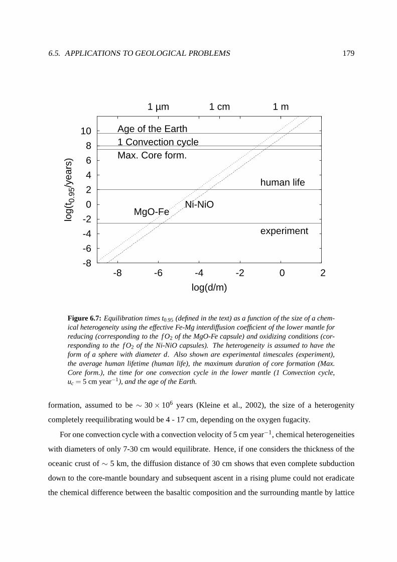
6.5. APPLICATIONS TO GEOLOGICAL PROBLEMS 179
-8
-6
-4
-2
0
2
4
6
8
10
-8 -6 -4 -2 0 2
1 µm 1 cm 1 m
log(
t 0.9
5/ye
ars)
log(d/m)
experiment
human life
Max. Core form.1 Convection cycleAge of the Earth
Ni-NiOMgO-Fe
Figure 6.7: Equilibration times t0.95 (defined in the text) as a function of the size of a chem-ical heterogeneity using the effective Fe-Mg interdiffusion coefficient of the lower mantle forreducing (corresponding to the f O2 of the MgO-Fe capsule) and oxidizing conditions (cor-responding to the f O2 of the Ni-NiO capsules). The heterogeneity is assumed to have theform of a sphere with diameter d. Also shown are experimentaltimescales (experiment),the average human lifetime (human life), the maximum duration of core formation (Max.Core form.), the time for one convection cycle in the lower mantle (1 Convection cycle,uc = 5 cm year−1), and the age of the Earth.
formation, assumed to be∼ 30× 106 years (Kleine et al., 2002), the size of a heterogenity
completely reequilibrating would be 4 - 17 cm, depending on the oxygen fugacity.
For one convection cycle with a convection velocity of 5 cm year−1, chemical heterogeneities
with diameters of only 7-30 cm would equilibrate. Hence, if one considers the thickness of the
oceanic crust of∼ 5 km, the diffusion distance of 30 cm shows that even completesubduction
down to the core-mantle boundary and subsequent ascent in a rising plume could not eradicate
the chemical difference between the basaltic composition and the surrounding mantle by lattice

180 CHAPTER 6. DISCUSSION
diffusion in the lower mantle. Because of the larger ionic radius and/or higher valence states of
radiogenic elements like Sr, Nd, Os or Re, these elements might have even smaller diffusion co-
efficients than the Fe-Mg interdiffusion coeffient and, hence, isotopic signatures of oceanic crust
and continental sediments will essentially be unaltered bydiffusion during convective recycling
in the lower mantle. More critical might be the interaction in the upper mantle where diffusion
properties are governed by olivine and its high-pressure polymorphs. The time to reach the 670
km discontinuity with a subduction rate of 5 cm year−1 is 1.3×10⁷ years. Even if the effec-
tive diffusion coefficient of the subducting slab would be 1×10⁻¹² m2 sec−1, corresponding to
wadsleyite (Figure 6.1), the maximum exchange distance would be on the order of 70 m. Hence,
considering that wadsleyite and ringwoodite are only stable in the transition zone and that olivine
might metastably survive in cold subduction zones, interaction in the upper mantle by pure lattice
diffusion also does not change significantly chemical heterogeneities during convection.
Over the entire history of the Earth (4.5× 10⁹ years), the diameter of heterogeneities that
would reequilibrate by lattice diffusion is 50 cm for reducing conditions and up to 2 m for more
oxidizing conditions. Clearly, heterogeneities larger than a few meters can survive several cycles
of convection in the lower mantle if the only exchange process is lattice diffusion. Extreme strain
rates would be required to stretch and subsequently thin heterogeneities to such an extent that
reequilibration would be possible. In two recent review papers (Van Keken et al., 2002, 2003)
numerical simulations are reported showing that convective mixing is vigorous enough to mix
large-scale heterogeneities. This conclusion is in contradiction to geochmical observations (e.g.
Hofmann, 1997). If one considers that even for extremeley large strains the ultimate reequilibra-
tion most likely would occur by diffusion, the very short reequilibration lengths obtained using
the Fe-Mg interdiffuision coefficents of this study providean explanation for the existence of
chemical heterogeneities.
For calculating the values given in this chapter a constant effective diffusion coefficient was
used (see above), which is only valid if the activation volume of diffusion is∼ 2 cm3 mol−1 as
calculated by Wright and Price (1989). As shown in Figure 6.2the Fe-Mg interdiffusion coef-
ficient of silicate perovskite would be increased approximately by a factor of 3000 in the lower
mantle if the activation volume is essentially zero. Therefore, the maximum increase of the in-

6.5. APPLICATIONS TO GEOLOGICAL PROBLEMS 181
teraction distances is a factor of√
3000≈ 55. This maximum increase of diffusivity shows that
the main conclusions of this section would be unaltered because the maximum size of a hetero-
geneity that can be reequilibrated over the entire history of the Earth would still be on the order
of only 100 m. Of course, grain boundary diffusion may have some additional effect to the dif-
fusion flux but this effect is difficult to estimate and most likely does not change the conclusions.
Only in a thermal boundary layer at the core-mantle boundaryare larger equilibration distances
possible, as shown in the next section.

182 CHAPTER 6. DISCUSSION
6.5.4 Interaction at the core-mantle boundary
Possible diffusive interaction at the core-mantle boundary is estimated using the effective dif-
fusion coefficient for a two phase aggregateDe f f = 2.4×Dpvsk whereDpvsk is the Fe-Mg in-
terdiffusion coefficient of silicate perovskite (Section 6.5.2). These calculations can be applied
to model reequilibration between the core and mantle for elements with diffusion coefficients
close to the Fe-Mg interdiffusion coefficient such as Fe, Ni or Co. A possible physical process
of reequilibration follows the formation of an FeO layer at the core-mantle boundary with sub-
sequent divalent cation exchange similar to the experimental setup in the experiments of Rubie
et al. (2000). The interaction lengthxdi f f is then given byxdi f f = 3.3√
De f f te (Equation 6.4),
wherete is the age of the Earth.
The pressure at the core-mantle boundary is approximately 136 GPa (Dziewonski and An-
derson, 1981) but the temperature is poorly constrained. A value of 3000 K on the mantle side
of the thermal boundary layer is derived from a mantle adiabat whereas for a core adiabat the
temperature at the core-mantle boundary might be as high as 5000 K (Williams, 1998). Most of
the parameters used in these estimates are highly uncertain, but according to Williams (1998) a
temperature contrast of 1000-2000 K across D” is likely. Forthe estimation of diffusion coeffi-
cients at the core-mantle boundary, 3000 K and 5000 K are adapted as limiting cases. According
to Boehler (1996) the melting temperature of ferropericlase at 136 GPa is also∼ 5000 K. For
silicate perovskite, several authors report melting temperatures in excess of 4000 K at around
60 GPa for Fe-free and Fe-bearing perovskite but no study hasbeen performed at pressures cor-
responding to the core mantle boundary (see review in Shen and Heinz, 1998). A theoretical
study of Wang (1999) predict a melting temperature of∼ 5000 K for MgSiO3 perovskite at the
core-mantle boundary. The oxygen fugacity relative to the iron-wustite buffer at the core-mantle
boundary (∆ f O2 ∼−2, Equation 5.20) should be close to the redox conditions of the experiments
employing MgO-Fe capsules (Section 5.5.2). Hence, Equation 5.21 was used for estimating the
Fe-Mg interdiffusion coefficient at the core mantle boundary.
In Table 6.2, the length of diffusive interactionxdi f f is calculated as outlined above. The
values ofxdi f f are on the order of 0.3 to 858 meters, depending on the activation volume and the
temperature. This interaction distance leads to the conclusion that, based on Fe-Mg interdiffusion
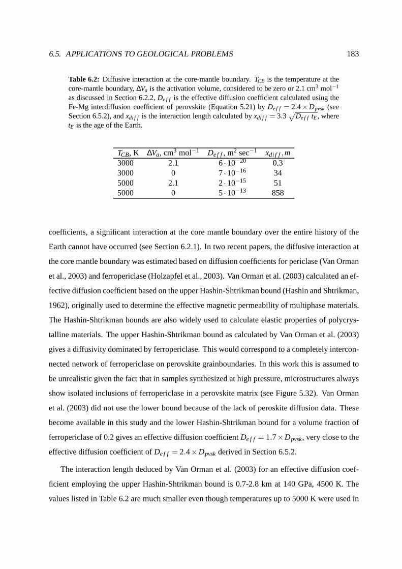
6.5. APPLICATIONS TO GEOLOGICAL PROBLEMS 183
Table 6.2: Diffusive interaction at the core-mantle boundary.TCB is the temperature at thecore-mantle boundary,∆Va is the activation volume, considered to be zero or 2.1 cm3 mol−1
as discussed in Section 6.2.2,De f f is the effective diffusion coefficient calculated using theFe-Mg interdiffusion coefficient of perovskite (Equation 5.21) by De f f = 2.4×Dpvsk (seeSection 6.5.2), andxdi f f is the interaction length calculated byxdi f f = 3.3
√
De f f tE, wheretE is the age of the Earth.
TCB, K ∆Va, cm3 mol−1 De f f, m2 sec−1 xdi f f ,m3000 2.1 6·10−20 0.33000 0 7·10−16 345000 2.1 2·10−15 515000 0 5·10−13 858
coefficients, a significant interaction at the core mantle boundary over the entire history of the
Earth cannot have occurred (see Section 6.2.1). In two recent papers, the diffusive interaction at
the core mantle boundary was estimated based on diffusion coefficients for periclase (Van Orman
et al., 2003) and ferropericlase (Holzapfel et al., 2003). Van Orman et al. (2003) calculated an ef-
fective diffusion coefficient based on the upper Hashin-Shtrikman bound (Hashin and Shtrikman,
1962), originally used to determine the effective magneticpermeability of multiphase materials.
The Hashin-Shtrikman bounds are also widely used to calculate elastic properties of polycrys-
talline materials. The upper Hashin-Shtrikman bound as calculated by Van Orman et al. (2003)
gives a diffusivity dominated by ferropericlase. This would correspond to a completely intercon-
nected network of ferropericlase on perovskite grainboundaries. In this work this is assumed to
be unrealistic given the fact that in samples synthesized athigh pressure, microstructures always
show isolated inclusions of ferropericlase in a perovskitematrix (see Figure 5.32). Van Orman
et al. (2003) did not use the lower bound because of the lack ofperoskite diffusion data. These
become available in this study and the lower Hashin-Shtrikman bound for a volume fraction of
ferropericlase of 0.2 gives an effective diffusion coefficientDe f f = 1.7×Dpvsk, very close to the
effective diffusion coefficient ofDe f f = 2.4×Dpvskderived in Section 6.5.2.
The interaction length deduced by Van Orman et al. (2003) foran effective diffusion coef-
ficient employing the upper Hashin-Shtrikman bound is 0.7-2.8 km at 140 GPa, 4500 K. The
values listed in Table 6.2 are much smaller even though temperatures up to 5000 K were used in

184 CHAPTER 6. DISCUSSION
addition to a larger proportionality factork in Equation 6.4. Only when an activation volume of
0 cm3 mol−1 is used, does the interaction distance at 5000 K become comparable to the values
of Van Orman et al. (2003). This is because, as shown in Figure6.2, the diffusion coefficient of
perovskite would then be smaller by a factor of only∼ 10 compared to ferropericlase. The in-
teraction distances using data for ferropericlase are on the order of 0.4 - 15 km for compositions
of XFeO= 0.1-0.2 and temperatures between 3000 and 5000 K at an oxygenfugacity close to
Ni-NiO buffer (Holzapfel et al., 2003).
Thus, it can be concluded that diffusive interaction at the core-mantle boundary is dominated
by diffusion in silicate perovskite leading to interactiondistances well below 1 km, hence, a
significant chemical interaction between the mantle and thecore based on Fe-Mg interdiffusion
coefficients can be excluded.
6.5. APPLICATIONS TO GEOLOGICAL PROBLEMS 185
6.5.5 Interaction during core formation
During early Earth’s history, the separation of a metallic phase from silicates/oxides occurred
which ultimately lead to the formation of the Earth’s core. Different modes of separation and the
physical processes involved are discussed by Stevenson (1990) and Rushmer et al. (2000).
Current models of core formation postulate equilibration between liquid silicate and liquid
Fe-alloy in a magma ocean with a depth of 700-1400 km. This is based on the observation that
partition coefficients at these conditions, for siderophile elements such as Ni and Co, achieve
values that can explain their abundance in the mantle and thecore (Thibault and Walter, 1995; Li
and Agee, 1996; Righter et al., 1997; Gessmann and Rubie, 2000; Li and Agee, 2001; Righter,
2003). The kinetics of equilibration of metal and silicate liquid in the magma ocean were dis-
cussed recently by Rubie et al. (2003).
Subsequently, after equilibration in the magma ocean, the liquid metal has to descend through
the solid lower mantle to form the core. It is still an open question whether this descent occurs in
the form of large diapirs or by percolation along grain boundaries due to grain boundary wetting.
The dihedral angle of core melts in lower mantle phases is approximately 71◦, considerably
smaller than for upper mantle phases (Shannon and Agee, 1998). Although this value is still
larger than the critical angle of 60◦, compositional effects or higher pressures might lower it
below the percolation threshold. The two different modes ofseparation are shown schematically
in Figure 6.8.
Because the partition coefficients of siderophile elementsare a function of pressure, temper-
ature and oxygen fugacity, their equilibrium distributionwill be different in the lower mantle
compared to the magma ocean. Hence, elements like Ni or Co will tend to be redistributed in
the lower mantle by exchange with Fe. Fe-Mg interdiffusion coefficients can be used as a proxy
for divalent cations such as Ni and Co as shown for the olivinesystem in Section 5.2. Also the
length of interaction of NiO with ferropericlase evident inFigure 5.23 indicates that the diffusion
coefficient of Ni is similar to that for Fe-Mg interdiffusion. A similar conclusion was reached
in the study of Rubie et al. (2000) in which the kinetics of equilibration between liquid metal
(initially oversaturated in oxygen) and MgO single crystalcapsules was investigated.
The length scales over which reequilibration has to occur are completely different in the two

186 CHAPTER 6. DISCUSSION
Proto-Core
Solidlowermantle
MagmaOcean
Percolationscenario
ponded liquidmetal
Diapirscenario
>100 km
0.1-1 mm
Figure 6.8: Current models of core formation postulate an equilibrium partitioning ofsiderophile elements at high pressure in a magma ocean. Subsequently, liquid metal sinksthrough the solid lower mantle to form the core either by large diapirs or by percolation dueto grain boundary wetting.
core forming scenarios shown in Figure 6.8. In the percolation process, the grain size of 0.1-
1 mm, estimated by Solomatov et al. (2002), is the dimension over which reequilibration has
to occur, whereas for a diapir model the characteristic length scale depends on the distanceXd
between individual diapirs. It is difficult to quantifyXd rigorously but according to a conservative
estimate it should be much larger than several kilometers. In the latter case, even on the timescale
of Earth’s history and temperatures as high as 5000 K a significant reequilibration of more than
1 km cannot occur using a two-phase model (Table 6.2). For∼ 30× 106 years, which is the
longest possible duration of core formation based on isotope constraints (Kleine et al., 2002),
equilibration distances in the lower mantle are< 1 m (Section 6.5.3). Thus, in a diapir scenario

6.5. APPLICATIONS TO GEOLOGICAL PROBLEMS 187
the composition of the lower mantle would not change significantly during final core formation.
The situation is much different in a percolation scenario. Even for relatively low tempera-
tures corresponding to a present day adiabat, 0.1 to 1 mm of equilibration can be realized on
timescales of less than 100000 years (Figure 6.7) using a two-phase model of the lower mantle
(Section 6.5.3). This is further illustrated in Figure 6.9.In the case of percolation, it is also
0
0.2
0.4
0.6
0.8
1
-1 0 1 2 3 4 5 6 7
χ
Log(Time/years)
0.1 mm
1 mm
2 mm
5 mm
Figure 6.9: Amount of reequilibrationχ (Equation 6.15) calculated using an effective diffu-sion coefficient for a two-phase aggregate composed of ferropericlase and silicate perovskitein a percolation szenario as a function of time and grainsizes between 0.1 and 5 mm. Seetext for further details.
possible to calculate the amount of reequilibration for silicate perovskite grains and ferroperi-
clase grains individually (because every grain is in contact with the metallic liquid) and then
average the results according to the phase abundance (20 vol% of ferropericlase and 80 vol% of
silicate perovskite, Poirier, 2000). In order to derive thereequilibration curves in Figure 6.9, the
distributionC(r) of a siderophile element in spherical grains of radiusrg employing Fe-Mg in-
terdiffusion coefficients as outlined in Section 6.2 and an analytical solution of Equation 1.2 was

188 CHAPTER 6. DISCUSSION
calculated (Equation 6.21 in Crank, 1979). For silicate perovskite only the model with an activa-
tion volume of 2.1 cm3 mol−1 was taken into account because in the case of∆Va = 0 cm3 mol−1
reequilibration would be even faster. The surface concentration of an individual grain was fixed
to a normalized concentration of 1 (taken to be the equilibrium value in contact with metallic
liquid), implicitly assuming that during reequilibration, the concentration of the metallic liquid
is not changed significantly and the bulk of the grain was initially at a normalized concentration
of zero. The first assumption is justified because of the siderophile nature of Ni and Co and a
corresponding much higher concentration of these elementsin the metallic liquid. To calculate
the amount of reequilibration, the average concentration of a grain with radiusrg at a certain
depth in the Earth is determined by:
ξ =1
43πr3
g
rgZ
r=0
C(r) 4πr2dr. (6.14)
Subsequently Equation 6.14 is integrated over the whole depth range of the lower mantle between
670 to 2900 km, to calculate the overall amount of reequilibration:
χ =1
Vlm
2900Z
x=670
ξ(d) 4πd2dx, (6.15)
whereVlm is the volume of the lower mantle between depthx of 670 and 2900 km.
The lower integration limit in Equation 6.15 corresponds tothe depth of former equilibra-
tion in the magma ocean. The results are not very sensitive with respect to this depth because,
due to the pressure effect of diffusion, the diffusion coefficients and therefore the amount of
reequilibration effectively do not change with depth (see Figure 6.2). Figure 6.9 shows that, if
metal separation occured by percolation, the equilibration signature in a magma ocean would
be completely destroyed within timescales much smaller than 100000 years and the present day
distribution of at least Ni and Co between the mantle and the core would correspond to a depth
integrated signature and not a single equilibration event in a magma ocean. However, partitioning
in the lower mantle for Ni and Co may not be much different fromin a magma ocean (Gessmann
and Rubie, 2000). On the other hand, this is unlikely to be thecase for all other siderophile
elements.
6.5. APPLICATIONS TO GEOLOGICAL PROBLEMS 189
It should be emphasized that the reequilibration times calculated by Equation 6.15 and shown
in Figure 6.9 are maximum values with respect to temperaturebecause a present day geotherm
(Anderson, 1982) was employed due to the high uncertaintiesof estimates of temperatures in the
early Earth. Temperatures might be significantly higher, for example on the order of 6000 K at
the bottom of a magma ocean, as pointed out by Karato and Murthy (1997). Diffusion would
have been much faster at these higher temperatures.

190 CHAPTER 6. DISCUSSION

Chapter 7
Conclusions
In this work, multianvil experiments have been performed inorder to study Fe-Mg interdiffusion
at high pressures in minerals relevant for the Earth’s interior. Single crystal and polycrystalline
diffusion couples were employed. It has been shown that the experimental technique employ-
ing the multianvil apparatus is capable of producing diffusion data with a high accuracy due to
temperature stability and low temperature gradients across the diffusion couples. Minerals in-
vestigated are olivine, wadsleyite, ferropericlase and (Mg,Fe)SiO3 perovskite. The conditions of
the experiments span a wide range of pressures between 6 and 26 GPa, temperatures between
1623 K and 2273 K at oxygen fugacity conditions close to the Ni-NiO buffer and, in the case of
silicate perovskite, at reducing conditions approximately 2 log-units below the Fe-wustite buffer.
The duration of the experiments ranged from 5 min to 72 hours resulting in profile lengths be-
tween 150 nm and 200µm. The longest profiles were observed in diffusion couples consisting
of wadsleyite and ferropericlase, whereas the shortest profiles were found in experiments em-
ploying silicate perovskite. Whereas profiles in olivine are just long enough to be measured by
electron microprobe analysis, profiles for silicate perovskite (< 1 µm) could only be measured
by analytical transmission electron microscopy employingan energy dispersive X-ray detector
(EDX-STEM). The combination of high pressure diffusion experiments with the analytical tech-
nique of EDX-STEM opens new perspectives of understanding diffusional properties of Earth
materials. Because of the much smaller Fe-Mg interdiffusion coefficients found in silicate per-
ovskite, which is assumed to be the major phase of the lower mantle, kinetic processes controlled
by Fe-Mg exchange occur on much longer timescales in the lower mantle compared to the up-
per mantle. Interaction between subducting slabs and the surrounding mantle by bulk diffusion
191

192 CHAPTER 7. CONCLUSIONS
is too slow to produce large scale homogenization even on timescales of convection overturn.
Significant chemical interaction at the core-mantle boundary during Earth’s history can be ex-
cluded based on Fe-Mg interdiffusion coefficients. Currentmodels of core formation involving
equilibration of metal and silicate in a magma ocean seem to predict abundances of siderophile
elements correctly if subsequent descent of the metal through the solid lower mantle occured
by large diapirs. In the case of percolation by grain boundary wetting extensive reequilibration
would be observed unless the distribution of siderophile elements between liquid metal and solid
ferropericlase and silicate perovskite is pressure-independent in the lower mantle.

Appendix A
Multianvil Technique
The multianvil technique employs a two-stage compression mechanism (Figure 2.1) for reducing
the areaA at nominally constant forceF to increase pressureP according to:
P =FA
(A.1)
Due to friction loss and the complicated geometry, as compared to opposing anvil designs, a
direct calculation of pressure is impossible. Thus, an experimental pressure calibration has to be
performed (Section 2.5), employing phase transitions of standard phases.
The main components of a multianvil system are (Figure 2.1):
• Hydraulic press generating a uniaxial force.
• first stage steel anvil system (cut from a sphere or cylinder)forming a cubic gap
• second stage WC cubes with truncated corners forming an octahedral pressure chamber
(Figure A.1)
• Octahedral pressure medium containing the sample.
In this study different hydraulic presses were used depending on the pressure of the experiment.
The different presses, their design and the pressure rangesinvestigated in this study are listed in
Table A.1.
In all cases sintered WC cubes (with a Co sinter additive) were used as second stage anvils
obtained from Toshiba tungaloy CO. LTD. (Japan) and WidiaValenite, Metalcutting Tools &
Fluids (Germany). They are isolated from the first stage steel anvils by epoxy sheets (Figure
193

194 APPENDIX A. MULTIANVIL TECHNIQUE
Table A.1: Presses installed at the Bayerisches Geoinstitut. The axial force is given inmeganewton. The multianvil designs (MA-design) are: Walker-type apparatus (Walker,Walker et al., 1990), split-sphere Kawai-type (split-sp, Kawai and Endo, 1970; Kawai et al.,1973), and split-cylinder (split-cy, Ohtani et al., 1987).P denotes the pressure range that wasstudied in a specific press employing diffusion couples of minerals given in the last column(ol = olivine, fp = ferropericlase, wds = wadsleyite, pvsk = silicate perovskite).
manufacturer force, MN MA-design P, GPa mineralVoggenreiter 5 Walker 6-12 ol
Hymag 10 split-cy 8-26 fp, wds, pvskSumitomo 12 split-sp 26 pvsk
Zwick 50 split-cy 22 pvsk
2.1). Only the two cubes that touch the upper and lower Mo discs of the assembly are brought
into contact with the steel anvil by means of a copper foil (Figure 2.1).
Figure A.2 shows schematically a 10/4 assembly. Details of all assemblies are shown in
Figure 2.2 and Figures 2.7-2.9. A copper coil protects the thermocouple in the gasket region
(Figure A.1). The thermocouple EMF is converted to temperature with a Eurotherm controler.
In multianvil experiments the temperature effect on the electromotive force of the thermo-
couple is usually neglected due to a lack of a correction method. The electromotive force (EMF)
of a thermocouple at high pressureP and temperatureT can be expressed as (Spain and Paauwe,
1977b; Walter et al., 1995):
EMF =
TogZ
Tre f
Sr(T,1 bar)dTdx
dx+
PexpZ
1 bar
TigZ
Tog
Sr(P,T)dTdx
dxdPdx
dx+
TexpZ
Tig
Sr(T,Pexp)dTdx
dx (A.2)
whereTre f is the reference temperature of the cold junction,x is the position along the circuit,Tog
is the temperature outside the gasket,Tig is the temperature on the high temperature side of the
gasket,Pexp andTexp are experimental pressure and temperature implicitely assuming that there
are no pressure gradients inside the assembly andSr is the relative Seebeck coefficient. Equation
A.2 shows that theEMF is not developed at the thermocouple junction but along the individual
wires wheredT/dx 6= 0 anddP/dx 6= 0. Therefore, any correction depends not only on the type
of thermocouple used but also on the temperature and pressure gradients across the gasket and
the temperature gradient in the assembly and therefore on the experimental configuration and
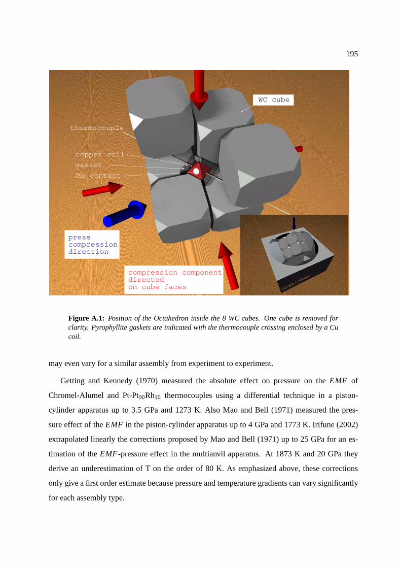
195
Copyright: C. Holzapfel
thermocouple
gasket
presscompressiondirection
compression componentdirectedon cube faces
copper coil
WC cube
Mo contact
Figure A.1: Position of the Octahedron inside the 8 WC cubes. One cube is removed forclarity. Pyrophyllite gaskets are indicated with the thermocouple crossing enclosed by a Cucoil.
may even vary for a similar assembly from experiment to experiment.
Getting and Kennedy (1970) measured the absolute effect on pressure on theEMF of
Chromel-Alumel and Pt-Pt90Rh10 thermocouples using a differential technique in a piston-
cylinder apparatus up to 3.5 GPa and 1273 K. Also Mao and Bell (1971) measured the pres-
sure effect of theEMF in the piston-cylinder apparatus up to 4 GPa and 1773 K. Irifune (2002)
extrapolated linearly the corrections proposed by Mao and Bell (1971) up to 25 GPa for an es-
timation of theEMF-pressure effect in the multianvil apparatus. At 1873 K and 20 GPa they
derive an underestimation of T on the order of 80 K. As emphasized above, these corrections
only give a first order estimate because pressure and temperature gradients can vary significantly
for each assembly type.

196 APPENDIX A. MULTIANVIL TECHNIQUE
Cop
yrig
ht: C
. Hol
zapf
el
MgO-octahedron
ZrO
2MgO
Mo
Al2O3
diffusion couple
thermocouple
LaCrO3
Figure A.2: Octahedron, cut open, to reveal the exact location of the thermocouple and theinner parts of the assembly. The inset is turne 180◦.
Instead of measuring the absolute pressure correction for theEMF, different authors tried to
determine the difference between different types of thermocouples (Ohtani et al., 1982; Kato and
Kumazawa, 1985; Tsuzaki and Takahashi, 1992; Walter et al.,1995). Ohtani et al. (1982) derived
a maximum deviation between a W-W75Re25 and a Pt-Pt87Rh13 thermocouple of 100 K. Using
values of Getting and Kennedy (1970) at 5 GPa and 2370 K the correction would be∼ 30 K
which is also the maximum deviation between the readings of aPt-Rh and W-Re thermocouple
in Walter et al. (1995). All evidence points to an underestimation of the real temperature in
multianvil experiments. Taking the various estimates of the pressure effect of the thermocouple
reading into account, the maximum underestimation of the absolute temperature is on the order
of 100 K.
197
Because all data at high pressure are subject to that temperature shift, the absolute value of
the activation energy determined in an Arrhenius plot wouldnot be affected if the EMF pressure
effect does not depend significantly on temperature. More critical is the determination of the
activation volume where data at high pressure are compared to literature data at 1 bar. For a
typical activation energy at 1 bar of 250 kJ mol−1 at a temperature of 1673 K and a temperature
underestimation of 100 K the corresponding underestimation of the activation volume would be
1.2 cm3 mol−1 comparing data at 1 bar and 12 GPa and 0.6 cm3 mol−1 using data at 1bar and 23
GPa. The real activation volume would be larger because the temperature of the experiment is
underestimated according to the proceeding discussion andthus for comparison at 1 bar (slower)
diffusivities at lower temperature would be used.

198 APPENDIX A. MULTIANVIL TECHNIQUE

Appendix B
TEMQuant: A program for quantifyingEDX-TEM analysis of ionic compounds
B.1 Principles of the program
Figure B.1 shows the principle algorithm of the program TEMQuant used for performing the
apsorption correction of EDX-STEM analysis following the procedure of Van Cappellen (1990)
and Van Cappellen and Doukhan (1994, for details see also Section 3.3). In section B.2 the
source code with some simplifications is given. Intensitiesare read from a data file provided by
the Vantage software. If TEMQuant is used for reading intensities written in other file formats
the class method readdat has to be changed according to the new format. For each data set (anal-
ysis) the uncorrected elemental ratios (relative to Si) arecalculated (Equation 3.1). Assuming
a density of 4 cm3 mol−1 and a take off angle of 15◦ an absorption corrected analysis is cal-
culated for a thickness of 10 nm (method StoichDicke). Usingthe electroneutrality constraint
of ionic compounds (Van Cappellen and Doukhan, 1994) the thickness is varied systematically
until the sum of charges of cations and anions is the same within error. Because the density and
take-off angle are not optimized the thickness is only an appararent thickness. This makes no
difference for the final result because it is the product of thickness, density, and take-off angle
which determines the apsorption-corrected k-factor in Equation 3.3.
199
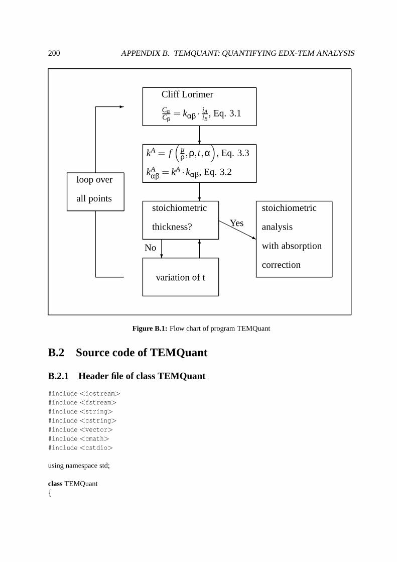
200 APPENDIX B. TEMQUANT: QUANTIFYING EDX-TEM ANALYSIS
Cliff Lorimer
CαCβ
= kαβ · iAiB
, Eq. 3.1
kA = f(
µρ ,ρ,t,α
)
, Eq. 3.3
kAαβ = kA ·kαβ, Eq. 3.2
stoichiometric
thickness?
No
Yes
variation of t
stoichiometric
analysis
with absorption
correction
loop over
all points
?
?
?
6
HHHHHHj
-
Figure B.1: Flow chart of program TEMQuant
B.2 Source code of TEMQuant
B.2.1 Header file of class TEMQuant
#include <iostream>#include <fstream>#include <string>#include <cstring>#include <vector>#include <cmath>#include <cstdio>
using namespace std;
classTEMQuant{

B.2. SOURCE CODE OF TEMQUANT 201
private:vector<int> feld; // intensitiesvector<double> intensitaeten;// intensities of elements of interest (e.g. not carbon from coating)vector<int> interesse;// localize elements;vector<string> elemente;// elementsymbols (2 characters!)unsigned intAnz Ele;// number of elements read from fileunsigned intAnz Analysen;// number of analysesdoubleMassAbsorption[30][30];// matrix of mass absorption coefficientsdoubleAtomicMass[100];// matrix of atomic massesdoublewertigkeit[100];// matrix of valencesvector<int> Ord Ele;// list of atomic numbers, only elements of interestunsigned intAnz Ord;// number of elements to be calculatedint PlatzSi; // position of Si in OrdEle?doublek factor[100];// k-faktors, at postion of atomic numbervector<double> konzentrationen;// weight percent of cationsvector<double> atomanteil;// atomic fraction of cationsvector<double> atomprozent;// atomic percent of cationsvector<double> KonzStoich;// composition calculated using algorithm of Van Capellen and
Doukhan (1994)vector<double> thickness;
public://construktorsTEMQuant(void);
// class methodsvoid readdat(char ∗name);vector<double> success(void); // gives back intensitaeten, to check if reading was succesfulvoid ausgabedatei(char ∗ausgabe);void zuordnung(void);doubleconcentration(double I1, double I2, doublek12); // Cliff-Lorimer-equationvoid norm(vector<double> & var); // normalization of concentration ratiovoid toAtom(vector<double> & konz); // normalization of a vektorvector<double> MassAbs(constvector<double> & conc);vector<double> acf(constvector<double> & massX,double thick);void absorption(double dicke, vector<double> & intensity); // calculates the composition of an
analysis without writing into private data membersvoid toAtom(void); // wt%→ atom%int StoichDicke(void); // calculates stoichiometric composition
};
B.2.2 Definition of class methods for class TEMQuant
#include ”TEMQuant.h”
using namespace std;
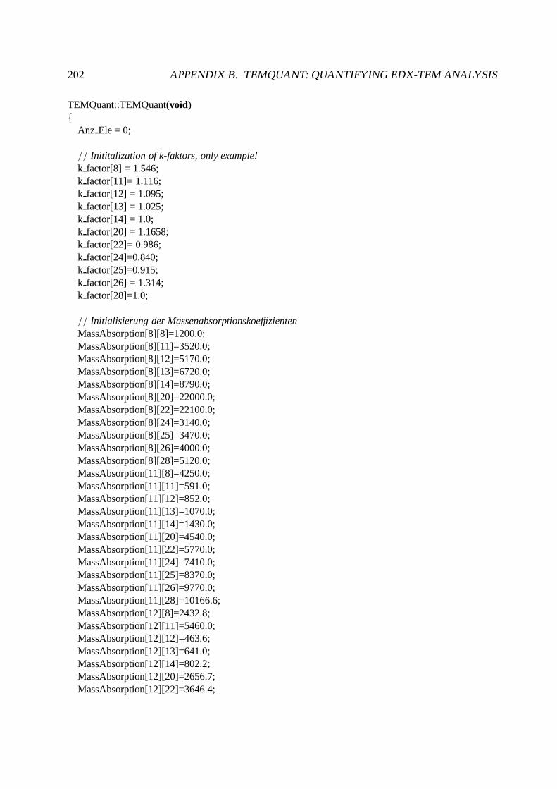
202 APPENDIX B. TEMQUANT: QUANTIFYING EDX-TEM ANALYSIS
TEMQuant::TEMQuant(void){
Anz Ele = 0;
// Inititalization of k-faktors, only example!k factor[8] = 1.546;k factor[11]= 1.116;k factor[12] = 1.095;k factor[13] = 1.025;k factor[14] = 1.0;k factor[20] = 1.1658;k factor[22]= 0.986;k factor[24]=0.840;k factor[25]=0.915;k factor[26] = 1.314;k factor[28]=1.0;
// Initialisierung der MassenabsorptionskoeffizientenMassAbsorption[8][8]=1200.0;MassAbsorption[8][11]=3520.0;MassAbsorption[8][12]=5170.0;MassAbsorption[8][13]=6720.0;MassAbsorption[8][14]=8790.0;MassAbsorption[8][20]=22000.0;MassAbsorption[8][22]=22100.0;MassAbsorption[8][24]=3140.0;MassAbsorption[8][25]=3470.0;MassAbsorption[8][26]=4000.0;MassAbsorption[8][28]=5120.0;MassAbsorption[11][8]=4250.0;MassAbsorption[11][11]=591.0;MassAbsorption[11][12]=852.0;MassAbsorption[11][13]=1070.0;MassAbsorption[11][14]=1430.0;MassAbsorption[11][20]=4540.0;MassAbsorption[11][22]=5770.0;MassAbsorption[11][24]=7410.0;MassAbsorption[11][25]=8370.0;MassAbsorption[11][26]=9770.0;MassAbsorption[11][28]=10166.6;MassAbsorption[12][8]=2432.8;MassAbsorption[12][11]=5460.0;MassAbsorption[12][12]=463.6;MassAbsorption[12][13]=641.0;MassAbsorption[12][14]=802.2;MassAbsorption[12][20]=2656.7;MassAbsorption[12][22]=3646.4;

B.2. SOURCE CODE OF TEMQUANT 203
MassAbsorption[12][24]=4782.0;MassAbsorption[12][25]=5443.6;MassAbsorption[12][26]=6120.7;MassAbsorption[12][28]=7709.5;MassAbsorption[13][8]=1503.3;MassAbsorption[13][11]=3359.4;MassAbsorption[13][12]=4376.5;MassAbsorption[13][13]=385.7;MassAbsorption[13][14]=503.4;MassAbsorption[13][20]=1667.0;MassAbsorption[13][22]=2288.0;MassAbsorption[13][24]=3000.5;MassAbsorption[13][25]=3415.6;MassAbsorption[13][26]=3840.6;MassAbsorption[13][28]=4837.5;MassAbsorption[14][8]=965.5;MassAbsorption[14][11]=2168.1;MassAbsorption[14][12]=2824.6;MassAbsorption[14][13]=3493.2;MassAbsorption[14][14]=327.9;MassAbsorption[14][20]=1086.0;MassAbsorption[14][22]=1490.6;MassAbsorption[14][24]=1954.8;MassAbsorption[14][25]=2225.3;MassAbsorption[14][26]=2502.1;MassAbsorption[14][28]=3151.6;MassAbsorption[20][8]=115.8;MassAbsorption[20][11]=265.9;MassAbsorption[20][12]=346.4;MassAbsorption[20][13]=431.7;MassAbsorption[20][14]=530.6;MassAbsorption[20][20]=139.4;MassAbsorption[20][22]=191.3;MassAbsorption[20][24]=250.8;MassAbsorption[20][25]=285.5;MassAbsorption[20][26]=321.1;MassAbsorption[20][28]=404.4;MassAbsorption[22][8]=65.7;MassAbsorption[22][11]=151.9;MassAbsorption[22][12]=197.9;MassAbsorption[22][13]=247.0;MassAbsorption[22][14]=304.3;MassAbsorption[22][20]=772.2;MassAbsorption[22][22]=110.6;MassAbsorption[22][24]=145.0;MassAbsorption[22][25]=165.1;MassAbsorption[22][26]=185.6;
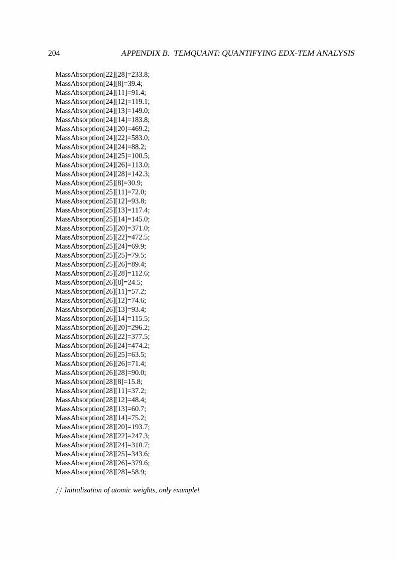
204 APPENDIX B. TEMQUANT: QUANTIFYING EDX-TEM ANALYSIS
MassAbsorption[22][28]=233.8;MassAbsorption[24][8]=39.4;MassAbsorption[24][11]=91.4;MassAbsorption[24][12]=119.1;MassAbsorption[24][13]=149.0;MassAbsorption[24][14]=183.8;MassAbsorption[24][20]=469.2;MassAbsorption[24][22]=583.0;MassAbsorption[24][24]=88.2;MassAbsorption[24][25]=100.5;MassAbsorption[24][26]=113.0;MassAbsorption[24][28]=142.3;MassAbsorption[25][8]=30.9;MassAbsorption[25][11]=72.0;MassAbsorption[25][12]=93.8;MassAbsorption[25][13]=117.4;MassAbsorption[25][14]=145.0;MassAbsorption[25][20]=371.0;MassAbsorption[25][22]=472.5;MassAbsorption[25][24]=69.9;MassAbsorption[25][25]=79.5;MassAbsorption[25][26]=89.4;MassAbsorption[25][28]=112.6;MassAbsorption[26][8]=24.5;MassAbsorption[26][11]=57.2;MassAbsorption[26][12]=74.6;MassAbsorption[26][13]=93.4;MassAbsorption[26][14]=115.5;MassAbsorption[26][20]=296.2;MassAbsorption[26][22]=377.5;MassAbsorption[26][24]=474.2;MassAbsorption[26][25]=63.5;MassAbsorption[26][26]=71.4;MassAbsorption[26][28]=90.0;MassAbsorption[28][8]=15.8;MassAbsorption[28][11]=37.2;MassAbsorption[28][12]=48.4;MassAbsorption[28][13]=60.7;MassAbsorption[28][14]=75.2;MassAbsorption[28][20]=193.7;MassAbsorption[28][22]=247.3;MassAbsorption[28][24]=310.7;MassAbsorption[28][25]=343.6;MassAbsorption[28][26]=379.6;MassAbsorption[28][28]=58.9;
// Initialization of atomic weights, only example!

B.2. SOURCE CODE OF TEMQUANT 205
AtomicMass[1]=1.00794;// insert other elements ...
// Initialization of valences, only example!wertigkeit[1]=1.0;// insert other elements ...
void TEMQuant::readdat(char ∗name){
ifstream indat(name);char inp[160];string test;string vergleich1, vergleich2;int i=1;int zahl,zeile=0;vergleich1= string("-Sigma)");vergleich2 = string("+/-");
// InitializationAnz Ele = 0;
// open fileif (indat)
{indat.getline(inp,160);while(!indat.eof())
{test=inp;if (test.find(vergleich1) != string::npos){
i++;}
if (test.find(vergleich2)!=string::npos){
if (i==2){
string str(test,2,4);elemente.pushback(str);
}test.erase(0,7);sscanf(test.cstr(),"%d",&zahl);feld.pushback(zahl);zeile++;// cout<< test<< ” ” << zahl<< endl;if (i==2) Anz Ele++;
}indat.getline(inp,160);
206 APPENDIX B. TEMQUANT: QUANTIFYING EDX-TEM ANALYSIS
}Anz Analysen = feld.size()/Anz Ele;
cout≪ "Anzahl der Analysen: "≪ Anz Analysen≪ endl;}
}
vector<double> TEMQuant::success(void){
vector<double> hilfe(intensitaeten);
return (hilfe);}
void TEMQuant::ausgabedatei(char ∗ausgabe){
ofstream outdat(ausgabe);unsigned int i;
if (outdat){
for (i = 0; i < elemente.size();i++) outdat≪ elemente[i]≪ " ";outdat≪ endl;for (i=0; i< feld.size();i++)
{outdat≪ feld[i] ≪ " ";if (i % Anz Ele == 6) outdat≪ endl;
}outdat≪ endl≪ endl≪ endl;outdat≪ "Nach van Capellen bestimmte Zusammensetzung: " ≪ endl;outdat≪ "anzahl analysen: "≪ Anz Analysen≪ endl;for (i=0; i<KonzStoich.size(); i++)
{if (i % Anz Ord == 0) outdat≪ i/Anz Ord+1≪ " ";outdat≪ KonzStoich[i]≪ " ";if (i % Anz Ord == Anz Ord-1) outdat≪ thickness[i/Anz Ord] ∗ 10000000.0≪ endl;if (i % (Anz Analysen∗Anz Ord) == Anz Analysen∗Anz Ord-1) outdat≪ endl≪ endl;
}}
}
void TEMQuant::zuordnung(void){
char test2;int test=0;unsigned int i,k;

B.2. SOURCE CODE OF TEMQUANT 207
int hilfsvar;double inttodouble;// Hilfsvariable// debugging:for (i=0; i<Ord Ele.size(); i++)
{cout≪ Ord Ele[i] ≪ endl;
}for (i=0; i<Anz Ele; i++)
{if (elemente[i]=="C -K")
{cout≪ "Element "≪ i ≪ "= " ≪ elemente[i]≪ endl;cout≪ "accept in matrix? - with y" ≪ endl;cin≫ test2;if (test2 == ’y’) {
test=1;} else{
test=0;}if (test == 1){
Ord Ele.pushback(6);interesse.pushback(i);
}}
if (elemente[i]=="Si-K"){
cout≪ "Element "≪ i ≪ "= " ≪ elemente[i]≪ endl;cout≪ "accept in matrix? - with y" ≪ endl;cin≫ test2;if (test2 == ’y’) {
test=1;} else{
test=0;}if (test == 1){
Ord Ele.pushback(14);interesse.pushback(i);
}}
// *************************************// do the same for all other elements// *************************************// where is Si?for (i=0; i<Ord Ele.size(); i++)
{
208 APPENDIX B. TEMQUANT: QUANTIFYING EDX-TEM ANALYSIS
if (Ord Ele[i]==14){
PlatzSi = i;}
} // implement control sequence!Anz Ord= OrdEle.size();for (i=0; i<Anz Analysen; i++)
{for (k=0; k<interesse.size(); k++)
{hilfsvar = feld[Anz Ele∗i+interesse[k]];inttodouble =double(hilfsvar);intensitaeten.pushback(inttodouble);
}}
// debugging:cout≪ "debug-information" ≪ endl;cout≪ Anz Ord≪ " Elemente" ≪ endl;for (i=0; i<Ord Ele.size(); i++)
{cout≪ Ord Ele[i] ≪ endl;
}cout≪ " Si an "≪ Platz Si+1≪ ". Stelle" ≪ endl;cout≪ " elemente standen an den plaetzen: "≪ endl;for (i = 0; i<interesse.size(); i++){
cout≪ interesse[i];}
}
doubleTEMQuant::concentration(double I1, double I2, doublek12){
doubleCAB;CAB = k12∗ I1/I2;return (CAB);
}
void TEMQuant::norm(vector<double> & var){
doublesumme = 0.0;unsigned int i;for (i=0; i<Anz Ord; i++){
summe = summe + var[i];}
for (i=0; i<Anz Ord; i++){var[i]=var[i]/summe;

B.2. SOURCE CODE OF TEMQUANT 209
}}
vector<double> TEMQuant::MassAbs(constvector<double> & conc){
unsigned int i,k;doubleabsor=0;vector<double> hilfe;for (i=0; i<conc.size(); i++){
for (k=0; k<conc.size(); k++){absor = absor + conc[k]∗MassAbsorption[OrdEle[i]][Ord Ele[k]];
}hilfe.pushback(absor);absor=0;
}
return (hilfe);}
vector<double> TEMQuant::acf(constvector<double> & massX,double thick){
doubledens=4.0;double takeoff=14.0∗3.1415926535/180.0;doublee1,e2,term1,fac;vector<double> E2,TERM1,factor;unsigned int i;e1 = 1-exp(-1∗ massX[PlatzSi]∗dens∗thick∗1/sin(takeoff));for (i=0; i<massX.size(); i++){
e2=1-exp(-1∗ massX[i]∗dens∗thick∗1/sin(takeoff));E2.pushback(e2);
}for (i=0; i<massX.size(); i++){
term1 = massX[i]/massX[PlatzSi];TERM1.pushback(term1);
}for (i=0; i<massX.size(); i++){
fac = e1/E2[i]∗TERM1[i];factor.pushback(fac);
}return (factor);
}
void TEMQuant::toAtom(void){
unsigned intk;unsigned int i,t;

210 APPENDIX B. TEMQUANT: QUANTIFYING EDX-TEM ANALYSIS
doublehilfe;vector<double> NurZurNormierung;for (i=0; i<konzentrationen.size()/Anz Ord; i++){
// konzentrationen might be larger than AnzAnalysen∗/for (k=0; k< Anz Ord; k++){
hilfe=konzentrationen[AnzOrd∗i+k]/AtomicMass[OrdEle[k]];atomanteil.pushback(hilfe);
}}for (i=0; i<atomanteil.size()/Anz Ord; i++){
NurZurNormierung.clear();for (k=0; k< Anz Ord; k++){
hilfe = atomanteil[AnzOrd∗i+k];NurZurNormierung.pushback(hilfe);
}norm(NurZurNormierung);for (t=0; t<NurZurNormierung.size(); t++){
atomprozent.pushback(NurZurNormierung[t]);}
}}
void TEMQuant::absorption(double dicke, vector<double> & intensity){
vector<double> intensity ratio,temp;vector<double> absorptions;vector<double> ACF;vector<double> kmod;// modified k-faktorunsigned intk;unsigned int t;double toleranz;// calculation of non-corrected intensity ratios (to Si)for (k=0; k<Anz Ord; k++)
{
intensity ratio.pushback(concentration(intensity[k],intensity[PlatzSi],k factor[Ord Ele[k]]));}
norm(intensityratio);
do {toleranz=0;kmod.clear();temp = intensityratio;absorptions = MassAbs(intensityratio);ACF = acf(absorptions, dicke);
B.2. SOURCE CODE OF TEMQUANT 211
for (t=0; t<Anz Ord; t++){kmod.pushback(ACF[t]∗k factor[Ord Ele[t]]);
}intensity ratio.clear();// clear, for optimized concentration ratiosfor (t=0; t<Anz Ord; t++){
intensity ratio.pushback(concentration(intensity[t],intensity[PlatzSi],kmod[t]));}norm(intensityratio);
for (t=0; t<Anz Ord; t++){toleranz=toleranz+fabs(intensityratio[t]-temp[t]);
}
} while (toleranz>0.000001);
// intensityratio → intensityintensity.clear();for (k=0; k<intensity ratio.size(); k++){
intensity.pushback(intensityratio[k]);}
}
void TEMQuant::toAtom(vector<double> & konz){
unsigned intk;// unsigned int i,t;doublehilfe;vector<double> NurZurNormierung;vector<double> atom;for (k=0; k< Anz Ord; k++){
hilfe=konz[k]/AtomicMass[OrdEle[k]];atom.pushback(hilfe);
}norm(atom);konz=atom;
}
int TEMQuant::StoichDicke(void){
unsigned int i,l;unsigned intk;int ende=0;// break conditiondoubledebug;// debug variabledoubleWieDick, add;// how thick is the sample, step sizedoublesumme1,summe2;// sum of charges, should become zerodoublehilfe; // help variablevector<double> datensatz;// for one data set

212 APPENDIX B. TEMQUANT: QUANTIFYING EDX-TEM ANALYSIS
vector<double> temporaer;// reset of datasetif (intensitaeten.empty()){
cout≪ "Kein Datensatz in atomprozent" ≪endl;return (-1);
}
KonzStoich.clear();thickness.clear();
// For each data setfor (i=0; i<intensitaeten.size()/Anz Ord; i++){
datensatz.clear();for (k=0; k<Anz Ord; k++){
hilfe = intensitaeten[AnzOrd∗i+k];datensatz.pushback(hilfe);
}WieDick = 0.000001;// start with 10 nmsumme1 = 0;summe2 = 0;temporaer = datensatz;absorption(WieDick,datensatz);toAtom(datensatz);
for (l=0; l<datensatz.size(); l++){hilfe = datensatz[l]∗wertigkeit[Ord Ele[l]];debug = datensatz[l];debug = wertigkeit[OrdEle[l]];summe1=summe1+hilfe;
}add = 0.00001;// 100 nm is first step sizedo{
ende++;// number of iterationsdatensatz = temporaer;
absorption(WieDick,datensatz);toAtom(datensatz);for (l=0; l<datensatz.size(); l++){
hilfe = datensatz[l]∗wertigkeit[Ord Ele[l]];summe2=summe2+hilfe;
}hilfe = summe1∗ summe2;// if hilfe <0 ist, change of signsif (hilfe < 0) add = -1∗add/2;summe1 = summe2;summe2 = 0;WieDick=WieDick+add;
} while (fabs(summe1)> 0.00000001 && ende< 100);if (ende>= 100) cout≪ endl≪ "MAXIMUM NUMBER OF ITERATIONS EXCEEDED" ≪ endl;

B.2. SOURCE CODE OF TEMQUANT 213
ende=0;cout≪ "AUSGABE VON ZWEITER BERECHNUNG" ≪ endl;cout≪ "Nr." ≪ i ≪ " ";for (k=0; k<Anz Ord; k++){
cout≪ datensatz[k]≪ " ";}cout≪ "d: "≪ WieDick;cout≪ endl;for (k=0; k<Anz Ord; k++){
KonzStoich.pushback(datensatz[k]);}thickness.pushback(WieDick);
}
return (0);}
B.2.3 Main function
#include ”TEMQuant.h”
int main(int argc,char ∗∗argv){
TEMQuant test;
if (argc == 1){cout≪ "usage: TEMQuant file" ≪ endl;cout≪ "end nothing else" ≪ endl;return (1);
}if (argc == 2){
test.readdat(argv[1]);}if (argc != 1 && argc != 2){
cout≪ "something wrong with file input, probably to much" ≪ endl;return (1);
}test.zuordnung();vector<double> suc(test.success());if (suc.empty()){
cout≪ "reading data was not succesfull" ≪ endl;return (2);
}test.toAtom();test.StoichDicke();test.ausgabedatei("raus.dat");

214 APPENDIX B. TEMQUANT: QUANTIFYING EDX-TEM ANALYSIS
return (0);}

Appendix C
ForwardLeastSquare: A program for finitedifference simulation of a diffusion profile
C.1 Introduction
The program ForwardLeastSquare calculates a finite difference simulation of a diffusion profile
assuming an exponential composition dependence (Equations 4.12 and 4.13). The simulated
profile can than be compared with an input data file containinga measured profile in order to
optimize the parametersD0 anda of Equation 4.12. The format of the ascii input file must be
”integer double”, otherwise reading of the data file resultsin an error. An option of the main
function allows to minimize the sum of squared deviations ofthe calculated and observed pro-
file. Due to the implementation of the minimization, the distance values of the measured profiles
must be integers. When converting noninteger distances to integer values by multiplying with
a suitable number one has to keep in mind to update the units ofthe diffusion coefficient. The
program calculates normalized concentrations. Therefore, the concentrations have to be normal-
ized prior least square minimization. For calculating the preexponential factor and asymmetry
parameter, an appropriate variable transformation must beperformed.
The main function allows several options. By choosing options 1-3 the standard values of
the number of space nodes (x), the preexponential factorD0 (d0) or the composition dependence
factora can be changed and directly calculated for a specific combination of timesteps (nt) and
factor (dt/dx2). This combination can be changed with option 5. Option 6-8 allow to optimize
one of the parametersx, d0 or a individually by minimizing the sum of squared deviations,
whereas option 9 optimizes all three parameters. The progress is monitored in a log-file and is
215

216 APPENDIX C. FINITE DIFFERENCE SIMULATION
continued for 1000 loops.
C.2 Source code
#include <iostream>#include <vector>#include <string>#include <fstream>#include <cmath>#include <cstdlib>#include <fstream>
using namespace std;
classleastsquare{private:
//////////////////////////////////////////////////////////////////// for calculation of profile//////////////////////////////////////////////////////////////////
int nt; // number of timestepsint nx; // number of x-nodesvector<double> neu m;vector<double> alt m;doublea;// asymmetry-factor, Eq. 4.12doublednull; // D0, Eq. 4.12double fak; // dt/dz2
/////////////////////////////////////////////////////////////////// for least square minimization////////////////////////////////////////////////////////////////
vector<long double> daten;// original datavector<long double> simuliert;// simulated data (take care on units)
public://///////////////////////////////////// Constructor////////////////////////////////////leastsquare(void);
////////////////////////////////////// calculation of profile///////////////////////////////////
C.2. SOURCE CODE 217
void calcProfile(void);
////////////////////////////////////// least square////////////////////////////////////void optimiseX(int initialx, int initialxstep);// change x: initialx→ initialx+initialxstep, comparison
of sum of squared deviations (ssr)void optimiseXsemiAuto(void); // minimize ssr by changing xvoid optimiseD0(double initialD0, double initialD0step);// change D0: initialD0 →
initialD0+initialD0step, comparison of ssrvoid optimiseD0semiAuto(void); // minimize ssr by changing D0void optimiseA(double initialA, double initialAstep);// change a: initiala→ initiala+initialastep,
comparison of sum of ssrvoid optimiseAsemiAuto(void); // minimize ssr by changing a
////////////////////////////////////// set-functions///////////////////////////////////void setParameters(void);
////////////////////////////////////// get-Funktionen///////////////////////////////////void getParameters(void);void print parametersinto file(void); // prints into filelong doublessr(void); // sum of squared residuals,∑
δx(Cm−Cs)
2, Section 4.3.2
};
leastsquare::leastsquare(){string filename;doublehilfe;
/////////////////////////////////////////////////////// Initialization for profile parameters////////////////////////////////////////////////////nt = 4100;nx=10;a=2.36;dnull=0.04;fak=0.5;
cout≪ "Name of original data" ≪ endl;cin ≫ filename;cout≪ filename≪ endl;
hilfe = 0.0;

218 APPENDIX C. FINITE DIFFERENCE SIMULATION
ifstream indat(filename.cstr());if (indat)
{while(!indat.eof()){
if (indat.eof()){break;
}indat≫ hilfe;daten.pushback(hilfe);}daten.popback();// because last element is to much
} else{cout≪ "no indat\n";
}
}
void leastsquare::calcProfile(void){int m=0,j=0;unsigned intausgabe;// for output of resultdoublehilfe; // when executing the finite differencesofstream aus("ausgabe.dat"); // output file
alt m.clear();neu m.clear();
/////////////////////////////////////// Initialization////////////////////////////////////while (m<nx){
if (m<nx/2){alt m.pushback(1.0);
} else{alt m.pushback(0.0);
}m+=1;
}
m=1;j=0;while (m<nt){
while (j<nx){
if (j==0) {neu m.pushback(1.0);// left boundary conditionj+=1;continue;

C.2. SOURCE CODE 219
}if (j==nx-1) {
neu m.pushback(0.0);// right boundary conditionj+=1;continue;
}// finite difference formulation, exp composition dependence, Eq. 4.13 and 4.18hilfe = alt m[j]+fak∗(1.0/4.0∗a∗dnull∗exp(a∗alt m[j])∗(alt m[j+1]-alt m[j-1])∗(alt m[j+1]-
alt m[j-1])+(dnull∗exp(a∗alt m[j]))∗(alt m[j+1]-2∗alt m[j]+alt m[j-1]));neu m.pushback(hilfe);j+=1;
}m+=1;// add 1 to mj=0; // reset jalt m.clear();// move elementsausgabe=0;while (ausgabe< neu m.size()){
alt m.pushback( neum[ausgabe]);// make new out of oldausgabe += 1;
}neu m.clear();
}
// outputausgabe = 0;while (ausgabe<alt m.size()){
aus≪ ausgabe≪ " "≪ alt m[ausgabe]≪ endl;ausgabe+=1;
}aus.close();
}
void leastsquare::setParameters(void){
cout≪ "number of timesteps" ≪ endl;cin ≫ nt;cout≪ "faktor: " ≪ endl;cin ≫ fak;
}
void leastsquare::getParameters(void){
cout≪ "current parameters" ≪ endl;cout≪ "number of timesteps: "≪ nt≪ endl;cout≪ "number of x-nodes: " ≪ nx ≪ endl;cout≪ "DO: "≪ dnull ≪ endl;cout≪ "asymmetriefactor: "≪ a≪ endl;
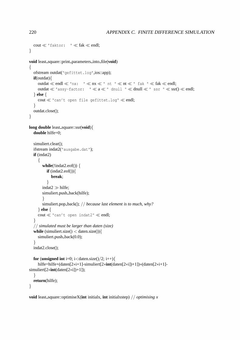
220 APPENDIX C. FINITE DIFFERENCE SIMULATION
cout≪ "faktor: " ≪ fak ≪ endl;}
void leastsquare::printparametersinto file(void){
ofstream outdat("gefittet.log",ios::app);if (outdat){
outdat≪ endl≪ "nx: "≪ nx ≪ " nt "≪ nt ≪ " fak "≪ fak ≪ endl;outdat≪ "assy-factor: "≪ a≪ " dnull "≪ dnull ≪ " ssr " ≪ ssr()≪ endl;
} else{cout≪ "can’t open file gefittet.log" ≪ endl;
}outdat.close();
}
long double leastsquare::ssr(void){doublehilfe=0;
simuliert.clear();ifstream indat2("ausgabe.dat");if (indat2)
{while(!indat2.eof()){
if (indat2.eof()){break;
}indat2≫ hilfe;simuliert.pushback(hilfe);}simuliert.popback();// because last element is to much, why?
} else{cout≪ "can’t open indat2" ≪ endl;
}// simulated must be larger than daten (size)while (simuliert.size()< daten.size()){
simuliert.pushback(0.0);}indat2.close();
for (unsigned int i=0; i<daten.size()/2; i++){hilfe=hilfe+(daten[2∗i+1]-simuliert[2∗int (daten[2∗i])+1])∗(daten[2∗i+1]-
simuliert[2∗int (daten[2∗i])+1]);}return (hilfe);
}
void leastsquare::optimiseX(int initialx, int initialxstep)// optimising x
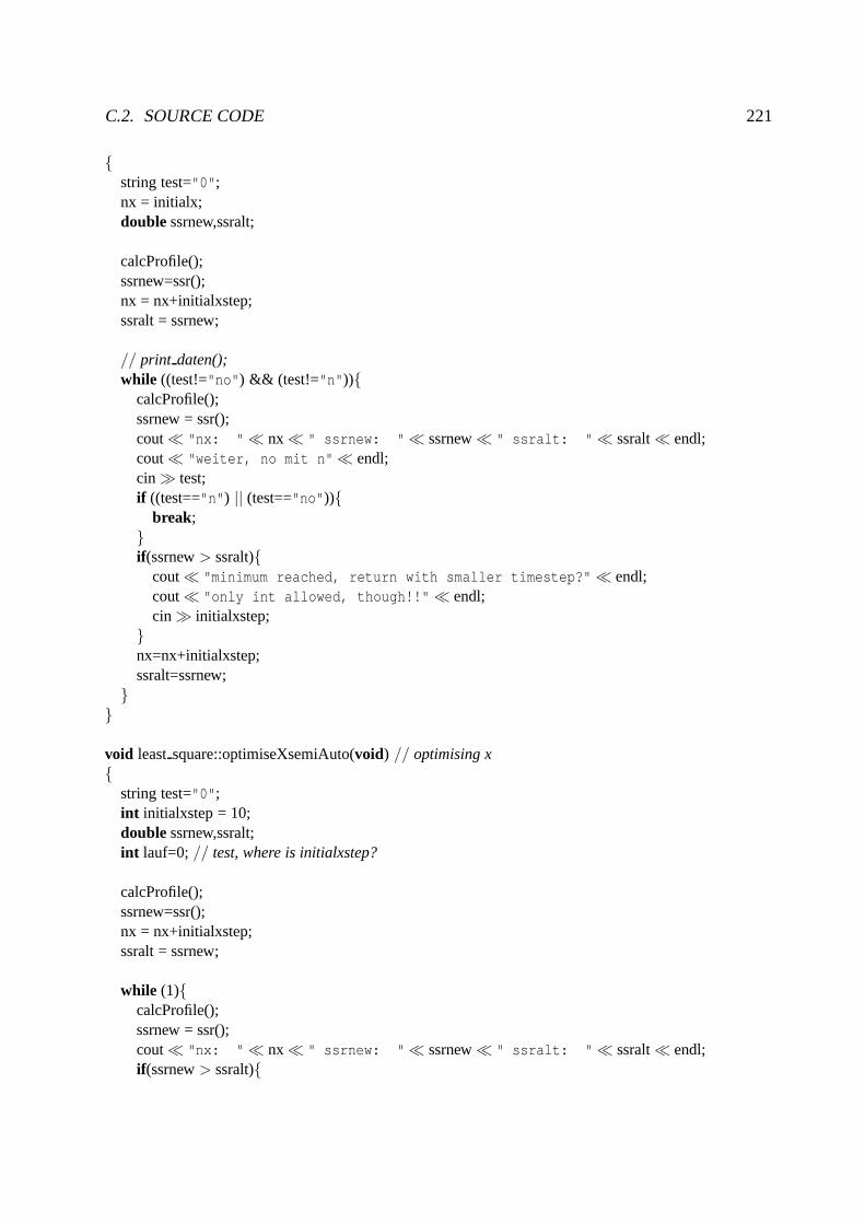
C.2. SOURCE CODE 221
{string test="0";nx = initialx;doublessrnew,ssralt;
calcProfile();ssrnew=ssr();nx = nx+initialxstep;ssralt = ssrnew;
// print daten();while ((test!="no") && (test!="n")){
calcProfile();ssrnew = ssr();cout≪ "nx: "≪ nx≪ " ssrnew: "≪ ssrnew≪ " ssralt: "≪ ssralt≪ endl;cout≪ "weiter, no mit n"≪ endl;cin ≫ test;if ((test=="n") || (test=="no")){
break;}if (ssrnew> ssralt){
cout≪ "minimum reached, return with smaller timestep?" ≪ endl;cout≪ "only int allowed, though!!" ≪ endl;cin ≫ initialxstep;
}nx=nx+initialxstep;ssralt=ssrnew;
}}
void leastsquare::optimiseXsemiAuto(void) // optimising x{
string test="0";int initialxstep = 10;doublessrnew,ssralt;int lauf=0;// test, where is initialxstep?
calcProfile();ssrnew=ssr();nx = nx+initialxstep;ssralt = ssrnew;
while (1){calcProfile();ssrnew = ssr();cout≪ "nx: "≪ nx≪ " ssrnew: "≪ ssrnew≪ " ssralt: "≪ ssralt≪ endl;if (ssrnew> ssralt){

222 APPENDIX C. FINITE DIFFERENCE SIMULATION
lauf=lauf+1;if (lauf==1){
initialxstep = -1;}if (lauf==2){
initialxstep =1;nx=nx+initialxstep;ssralt=ssrnew;calcProfile();ssrnew = ssr();cout≪ "nx: "≪ nx ≪ " ssrnew: "≪ ssrnew≪ " ssralt: "≪ ssralt≪ endl;break;
}}nx=nx+initialxstep;ssralt=ssrnew;
}}
void leastsquare::optimiseD0(double initialD0, double initialD0step)// optimising D0{
string test="0";dnull = initialD0;doublessrnew,ssralt;
calcProfile();ssrnew=ssr();dnull = dnull+initialD0step;ssralt = ssrnew;
while ((test!="no") && (test!="n")){calcProfile();ssrnew = ssr();cout≪ "D0: "≪ dnull ≪ "step: "≪ initialD0step≪ " ssrnew: "≪ ssrnew≪ "
ssralt: "≪ ssralt≪ endl;cout≪ "weiter, no mit n"≪ endl;cin ≫ test;if ((test=="n") || (test=="no")){
break;}if (ssrnew> ssralt){
cout≪ "minimum reached, return with smaller D0step?" ≪ endl;cin ≫ initialD0step;
}dnull=dnull+initialD0step;ssralt=ssrnew;
}
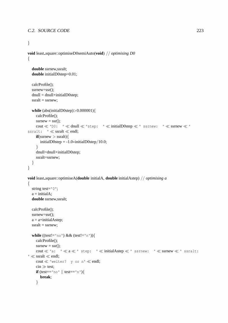
C.2. SOURCE CODE 223
}
void leastsquare::optimiseD0semiAuto(void) // optimising D0{
doublessrnew,ssralt;double initialD0step=0.01;
calcProfile();ssrnew=ssr();dnull = dnull+initialD0step;ssralt = ssrnew;
while (abs(initialD0step)>0.000001){calcProfile();ssrnew = ssr();cout≪ "D0: "≪ dnull ≪ "step: "≪ initialD0step≪ " ssrnew: "≪ ssrnew≪ "
ssralt: "≪ ssralt≪ endl;if (ssrnew> ssralt){
initialD0step = -1.0∗initialD0step/10.0;}dnull=dnull+initialD0step;ssralt=ssrnew;
}}
void leastsquare::optimiseA(double initialA, double initialAstep)// optimising a{
string test="0";a = initialA;doublessrnew,ssralt;
calcProfile();ssrnew=ssr();a = a+initialAstep;ssralt = ssrnew;
while ((test!="no") && (test!="n")){calcProfile();ssrnew = ssr();cout≪ "a: "≪ a≪ " step: "≪ initialAstep≪ " ssrnew: "≪ ssrnew≪ " ssralt:
"≪ ssralt≪ endl;cout≪ "weiter? y or n" ≪ endl;cin ≫ test;if (test=="no" || test=="n"){
break;}

224 APPENDIX C. FINITE DIFFERENCE SIMULATION
if (ssrnew> ssralt){cout≪ "minimum reached, return with smaller Astep?" ≪ endl;cin ≫ initialAstep;
}a=a+initialAstep;ssralt=ssrnew;
}}
void leastsquare::optimiseAsemiAuto(void) // optimising a{
doublessrnew,ssralt;double initialAstep=0.1;
calcProfile();ssrnew=ssr();a = a+initialAstep;ssralt = ssrnew;
while (abs(initialAstep)> 0.00001){calcProfile();ssrnew = ssr();cout≪ "a: "≪ a≪ " step: "≪ initialAstep≪ " ssrnew: "≪ ssrnew≪ " ssralt:
"≪ ssralt≪ endl;if (ssrnew> ssralt){
initialAstep = -1.0∗initialAstep/10.0;}a=a+initialAstep;ssralt=ssrnew;
}}
int main(int argc,char ∗∗argv){
string auswahl;int startX,incrementX;doublestartD0,incrementD0,starta,incrementa;cout≪ "program for least square of numerical fits" ≪ endl;leastsquare profileObject;while (1){
cout≪ "What do you want to do?" ≪ endl;cout≪ "there are several choices: "≪ endl;cout≪ "1 = optimise x" ≪ endl;cout≪ "2 = optimise d0" ≪ endl;cout≪ "3 = optimise a" ≪ endl;cout≪ "4 = terminate program" ≪ endl;cout≪ "5 = set nt and faktor" ≪ endl;

C.2. SOURCE CODE 225
cout≪ "6 = semiauto refinement of x" ≪ endl;cout≪ "7 = semiauto refinement of a" ≪ endl;cout≪ "8 = semiauto refinement of D0" ≪ endl;cout≪ "9 = 1000 durchgaenge" ≪ endl;cout≪ endl;profileObject.getParameters();cout≪ endl;cin ≫ auswahl;if ((auswahl !="1") && (auswahl !="2") && (auswahl !="3") && (auswahl !="4") &&
(auswahl !="5") && (auswahl !="6") && (auswahl !="7") && (auswahl !="8") && (auswahl !="9")){
cout≪ "Mmmmh..." ≪ endl;cout≪ "didn’t I say something of giving a number" ≪ endl;cout≪ "between 1 and 9?" ≪ endl;cout≪ "next time I would try this" ≪ endl;continue;
}if (auswahl =="1"){
cout≪ "startX incrementX" ≪ endl;cin ≫ startX≫ incrementX;profileObject.optimiseX(startX,incrementX);
}if (auswahl =="2"){
cout≪ "startD0 incrementD0" ≪ endl;cin ≫ startD0≫ incrementD0;profileObject.optimiseD0(startD0,incrementD0);
}if (auswahl =="3"){
cout≪ "starta incrementa" ≪ endl;cin ≫ starta≫ incrementa;profileObject.optimiseA(starta,incrementa);
}if (auswahl =="4"){
return (0);}if (auswahl =="5"){
profileObject.setParameters();}if (auswahl =="6"){
profileObject.optimiseXsemiAuto();}if (auswahl =="7"){
profileObject.optimiseAsemiAuto();}if (auswahl =="8"){
profileObject.optimiseD0semiAuto();}

226 APPENDIX C. FINITE DIFFERENCE SIMULATION
if (auswahl =="9"){int zaehler = 0;for (zaehler = 0; zaehler< 1000; zaehler++){
profileObject.optimiseXsemiAuto();profileObject.optimiseD0semiAuto();profileObject.optimiseAsemiAuto();profileObject.printparametersinto file();
}}
}}

Appendix D
Example profile analyses
In this section, example diffusion profile analyses also given in the Figures in Chapter 3 are
listed. Profile analysis was performed either by electron microprobe (EPMA) or with enery
dispersive X-ray spectrometry on a transmission electron microscope (EDX-STEM) as discussed
in Chapter 5.
227

228 APPENDIX D. EXAMPLE PROFILE ANALYSES
Table D.1: Profile analysis for olivine shown in Fig. 5.3 measured with EPMA. The experi-ment was performed at 12 GPa, 1623 K and annealed for 72 h. All concentrations are givenin weight percent of the oxide.
Distance,µm MgO SiO2 MnO FeO NiO Sum0 51.67 41.66 0.179 6.46 0.237 100.201 51.59 41.95 0.178 6.21 0.251 100.182 51.38 41.34 0.174 6.27 0.244 99.403 51.69 41.67 0.164 6.29 0.267 100.084 51.41 41.55 0.172 6.33 0.232 99.705 51.30 41.76 0.151 6.25 0.279 99.746 51.59 41.46 0.148 6.36 0.263 99.827 51.38 41.52 0.155 6.34 0.251 99.648 51.51 41.43 0.139 6.21 0.239 99.539 51.60 41.32 0.148 6.19 0.277 99.5310 51.46 41.43 0.146 6.24 0.248 99.5311 51.59 41.51 0.141 6.22 0.232 99.6912 51.58 41.67 0.165 6.28 0.269 99.9613 51.74 41.59 0.155 5.96 0.269 99.7014 52.25 41.64 0.134 5.78 0.227 100.0315 52.37 41.73 0.118 5.43 0.215 99.8616 52.69 41.78 0.116 4.82 0.213 99.6117 52.88 41.70 0.096 4.33 0.201 99.2118 53.39 41.82 0.080 3.70 0.187 99.1819 53.94 42.00 0.085 2.94 0.141 99.1120 54.59 42.26 0.063 2.16 0.073 99.1521 55.02 42.49 0.071 1.50 0.038 99.1122 55.66 42.42 0.018 0.94 0.061 99.1123 56.14 42.70 0.000 0.39 0.037 99.2724 56.06 42.74 0.009 0.18 0.006 99.0025 56.27 42.98 0.000 0.14 0.000 99.3726 56.24 42.72 0.000 0.08 0.017 99.0527 56.11 42.90 0.000 0.12 0.000 99.1328 56.34 42.69 0.003 0.10 0.009 99.1429 56.19 43.00 0.000 0.04 0.011 99.2530 56.34 42.87 0.008 0.10 0.018 99.3431 56.32 42.82 0.000 0.06 0.000 99.2032 56.34 43.05 0.013 0.12 0.018 99.5433 56.49 43.10 0.005 0.12 0.032 99.7534 56.35 42.66 0.019 0.08 0.018 99.1335 56.32 42.83 0.001 0.06 0.000 99.2236 56.37 42.87 0.009 0.06 0.000 99.3137 56.10 42.92 0.006 0.06 0.010 99.1038 56.35 43.00 0.012 0.05 0.014 99.4339 56.28 42.95 0.008 0.06 0.045 99.3440 56.16 42.82 0.005 0.06 0.034 99.08

229
Table D.2: Profile analysis for olivine shown in Fig. 5.4-A measured with EDX-STEM. Theexperiment was performed at 10 GPa, 1673 K and annealed for 24h. All concentrations aregiven in atom%. EDX analyses are normalized to 100%
distance O Mg Si Fe distance O Mg Si Fe14 56.59 30.22 13.17 0.0236.8 56.73 28.95 13.45 0.87513.8 56.63 30.09 13.26 0.0226.6 56.77 28.85 13.53 0.85313.6 56.68 29.95 13.36 0.0076.4 56.77 28.79 13.55 0.89013.4 56.77 29.69 13.54 0.0106.2 56.84 28.55 13.69 0.91513.2 56.72 29.85 13.43 0.0076 56.87 28.42 13.74 0.97413 56.79 29.61 13.58 0.0215.8 56.69 28.96 13.38 0.97712.8 56.70 29.88 13.40 0.0245.6 56.81 28.53 13.63 1.03012.6 56.62 30.11 13.24 0.0305.4 56.81 28.46 13.62 1.10712.4 56.60 30.18 13.21 0.0115.2 56.86 28.31 13.72 1.11112.2 56.73 29.81 13.45 0.0125 56.82 28.39 13.65 1.14512 56.67 29.95 13.34 0.0324.8 56.83 28.37 13.67 1.12611.8 56.72 29.81 13.44 0.0374.6 56.87 28.26 13.73 1.13911.6 56.73 29.80 13.46 0.0084.4 56.77 28.65 13.54 1.04111.4 56.60 30.17 13.19 0.0464.2 56.89 28.22 13.77 1.11811.2 56.67 29.92 13.34 0.0654 56.79 28.47 13.58 1.15011 56.74 29.71 13.48 0.0743.8 56.84 28.21 13.68 1.26810.8 56.76 29.63 13.51 0.1013.6 56.88 27.99 13.77 1.36310.6 56.71 29.76 13.42 0.1083.4 56.84 28.13 13.67 1.36410.4 56.65 29.94 13.30 0.1153.2 56.94 27.76 13.87 1.43110.2 56.77 29.55 13.54 0.1393 56.98 27.66 13.95 1.41310 56.79 29.49 13.57 0.1442.8 57.15 27.26 14.30 1.2979.8 56.70 29.67 13.41 0.2182.6 57.00 27.60 14.00 1.3999.6 56.74 29.51 13.49 0.2582.4 56.97 27.71 13.94 1.3819.4 56.84 29.21 13.68 0.2792.2 56.88 27.95 13.76 1.4019.2 56.88 29.12 13.76 0.2472 56.89 27.85 13.78 1.4829 56.77 29.35 13.54 0.3411.8 56.74 28.42 13.49 1.3498.8 56.77 29.34 13.54 0.3491.6 56.88 27.93 13.76 1.4308.6 56.72 29.42 13.44 0.4261.4 56.85 28.03 13.70 1.4238.4 56.78 29.15 13.57 0.4971.2 56.77 28.30 13.54 1.3858.2 56.90 28.80 13.81 0.4871 56.89 27.88 13.78 1.4448 56.64 29.57 13.27 0.5210.8 56.83 28.05 13.66 1.4657.8 56.86 28.88 13.72 0.5460.6 56.90 27.84 13.79 1.4707.6 56.54 29.75 13.08 0.6310.4 56.86 27.94 13.72 1.4827.4 57.08 28.12 14.17 0.6280.2 56.77 28.20 13.54 1.4987.2 56.93 27.71 13.87 1.4860 56.81 28.09 13.63 1.4637 56.94 28.39 13.87 0.800

230 APPENDIX D. EXAMPLE PROFILE ANALYSES
Table D.3: Profile analysis for olivine shown in Fig. 5.4-B measured with EDX-STEM. Theexperiment was performed at 12 GPa, 1673 K and annealed for 24h. All concentrations aregiven in atom%. EDX analyses are normalized to 100%
distance,µm O Mg Si Fe Ni Mn0 57.29 26.32 14.53 1.706 0.107 0.0520.5 57.35 26.14 14.63 1.718 0.105 0.0571 57.31 26.22 14.59 1.731 0.101 0.0371.5 57.35 26.16 14.67 1.720 0.071 0.0322 57.36 26.13 14.67 1.699 0.094 0.0542.5 57.25 26.47 14.44 1.668 0.098 0.0713 57.20 26.62 14.37 1.683 0.090 0.0413.5 57.22 26.53 14.39 1.716 0.109 0.0444 57.22 26.58 14.37 1.694 0.081 0.0594.5 57.23 26.55 14.41 1.663 0.105 0.0395 57.29 26.46 14.54 1.562 0.109 0.0405.5 57.25 26.70 14.44 1.475 0.087 0.0526 57.14 27.00 14.24 1.507 0.069 0.0426.5 57.26 26.89 14.48 1.264 0.077 0.0347 57.24 27.09 14.45 1.108 0.094 0.0247.5 57.42 26.91 14.81 0.797 0.040 0.0228 57.28 27.34 14.54 0.768 0.059 0.0178.5 57.08 28.13 14.14 0.573 0.058 0.0139 56.90 28.81 13.80 0.466 0.016 0.0029.5 57.10 28.35 14.18 0.325 0.036 0.01510 56.99 28.80 13.98 0.179 0.043 0.00210.5 56.81 29.47 13.60 0.068 0.049 0.01511 57.09 28.66 14.18 0.028 0.038 0.00411.5 56.97 29.05 13.94 0.016 0.029 0.00012 57.06 28.76 14.12 0.021 0.036 0.00012.5 57.65 27.00 15.29 0.024 0.035 0.00013 57.12 28.58 14.23 0.027 0.043 0.00013.5 57.21 28.31 14.42 0.014 0.042 0.00214 57.17 28.44 14.34 0.022 0.019 0.00614.5 57.21 28.33 14.42 0.015 0.021 0.00015 57.08 28.72 14.14 0.016 0.031 0.014

231
Table D.4: Profile analysis for wadsleyite shown in Fig. 5.18 measured with EPMA. The ex-periment was performed at 15 GPa, 1773 K and annealed for 16 minutes. All concentrationsare given in weight percent of the oxide.
d, µm MgO SiO2 FeO NiO Sum d, µm MgO SiO2 FeO NiO Sum500 55.61 43.05 0.049 0.000 98.71556 56.49 42.34 0.113 0.000 98.94501 55.87 42.71 0.085 0.055 98.72557 56.08 42.52 0.133 0.013 98.75504 56.06 42.23 0.058 0.025 98.37559 55.63 42.13 0.179 0.067 98.01505 56.17 42.13 0.091 0.067 98.46560 56.14 42.41 0.215 0.032 98.80506 56.11 42.16 0.035 0.017 98.32561 55.75 42.11 0.143 0.090 98.10507 55.94 42.13 0.049 0.023 98.15562 55.77 42.30 0.178 0.087 98.33508 56.46 42.38 0.072 0.025 98.93563 56.13 42.73 0.279 0.000 99.14511 56.45 41.99 0.090 0.029 98.56564 55.30 43.39 0.160 0.006 98.85512 56.08 42.14 0.030 0.029 98.28568 55.71 42.60 0.516 0.122 98.95513 55.98 42.26 0.126 0.029 98.40569 55.25 42.42 0.718 0.036 98.43514 56.31 42.39 0.100 0.087 98.88570 55.79 42.16 0.926 0.061 98.93515 56.19 42.65 0.081 0.064 98.99571 54.47 42.87 1.128 0.010 98.48517 55.97 42.23 0.077 0.004 98.28574 54.72 41.92 2.184 0.067 98.90518 56.24 42.20 0.072 0.055 98.57575 54.85 41.93 2.451 0.095 99.33519 55.79 42.28 0.059 0.000 98.13576 54.47 41.81 2.893 0.032 99.20520 55.75 42.25 0.058 0.004 98.06577 53.90 41.62 3.495 0.000 99.01521 55.77 42.19 0.059 0.051 98.07579 53.00 41.42 4.299 0.080 98.80522 56.67 42.17 0.077 0.025 98.94580 52.67 41.56 4.666 0.070 98.96523 56.16 42.28 0.084 0.116 98.64581 52.58 41.36 5.034 0.051 99.02524 56.22 42.13 0.068 0.048 98.47582 52.05 41.11 5.654 0.010 98.82525 55.53 42.95 0.000 0.070 98.54583 51.93 40.85 6.018 0.118 98.93526 52.67 45.42 0.134 0.048 98.28584 51.20 40.79 6.255 0.042 98.28527 55.72 42.93 0.046 0.000 98.70585 51.19 41.07 7.089 0.048 99.39528 56.23 42.32 0.064 0.000 98.61586 50.83 40.89 7.270 0.115 99.10541 56.12 42.22 0.120 0.010 98.47587 50.51 40.57 7.763 0.137 98.98542 56.07 42.29 0.109 0.051 98.51588 50.05 40.69 8.203 0.130 99.06543 56.46 42.10 0.078 0.000 98.64589 49.61 40.57 8.435 0.134 98.75544 56.46 42.43 0.111 0.042 99.04590 49.34 40.34 8.998 0.092 98.77545 56.25 42.05 0.096 0.048 98.45591 49.20 40.44 9.587 0.286 99.51546 56.39 42.18 0.091 0.000 98.66594 47.92 39.93 10.275 0.289 98.41547 56.63 42.04 0.133 0.000 98.80595 48.11 40.15 10.879 0.153 99.29548 55.98 42.62 0.104 0.064 98.76596 47.43 40.27 10.792 0.193 98.69549 53.47 45.15 0.207 0.025 98.85597 47.42 40.07 11.017 0.266 98.77550 56.63 42.49 0.169 0.036 99.32598 47.41 40.06 11.231 0.317 99.01551 56.37 42.47 0.126 0.055 99.03599 47.13 40.00 11.425 0.234 98.79552 56.36 42.34 0.149 0.019 98.87600 46.74 39.88 11.783 0.221 98.62553 56.24 42.30 0.152 0.000 98.69601 47.00 39.71 11.868 0.313 98.88554 56.02 42.38 0.122 0.000 98.52602 46.84 39.81 12.117 0.225 98.99555 56.35 42.25 0.091 0.090 98.78603 46.69 39.91 12.228 0.307 99.13
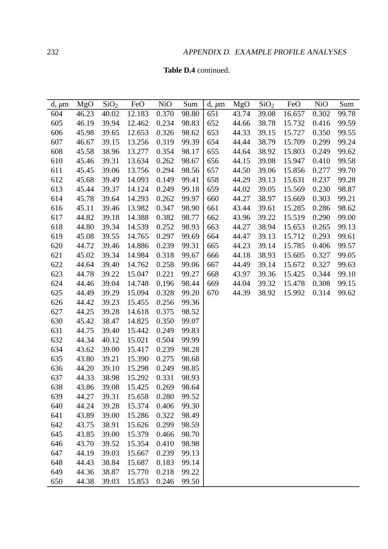
232 APPENDIX D. EXAMPLE PROFILE ANALYSES
Table D.4continued.
d, µm MgO SiO2 FeO NiO Sum d, µm MgO SiO2 FeO NiO Sum604 46.23 40.02 12.183 0.370 98.80651 43.74 39.08 16.657 0.302 99.78605 46.19 39.94 12.462 0.234 98.83652 44.66 38.78 15.732 0.416 99.59606 45.98 39.65 12.653 0.326 98.62653 44.33 39.15 15.727 0.350 99.55607 46.67 39.15 13.256 0.319 99.39654 44.44 38.79 15.709 0.299 99.24608 45.58 38.96 13.277 0.354 98.17655 44.64 38.92 15.803 0.249 99.62610 45.46 39.31 13.634 0.262 98.67656 44.15 39.08 15.947 0.410 99.58611 45.45 39.06 13.756 0.294 98.56657 44.50 39.06 15.856 0.277 99.70612 45.68 39.49 14.093 0.149 99.41658 44.29 39.13 15.631 0.237 99.28613 45.44 39.37 14.124 0.249 99.18659 44.02 39.05 15.569 0.230 98.87614 45.78 39.64 14.293 0.262 99.97660 44.27 38.97 15.669 0.303 99.21616 45.11 39.46 13.982 0.347 98.90661 43.44 39.61 15.285 0.286 98.62617 44.82 39.18 14.388 0.382 98.77662 43.96 39.22 15.519 0.290 99.00618 44.80 39.34 14.539 0.252 98.93663 44.27 38.94 15.653 0.265 99.13619 45.08 39.55 14.765 0.297 99.69664 44.47 39.13 15.712 0.293 99.61620 44.72 39.46 14.886 0.239 99.31665 44.23 39.14 15.785 0.406 99.57621 45.02 39.34 14.984 0.318 99.67666 44.18 38.93 15.605 0.327 99.05622 44.64 39.40 14.762 0.258 99.06667 44.49 39.14 15.672 0.327 99.63623 44.78 39.22 15.047 0.221 99.27668 43.97 39.36 15.425 0.344 99.10624 44.46 39.04 14.748 0.196 98.44669 44.04 39.32 15.478 0.308 99.15625 44.49 39.29 15.094 0.328 99.20670 44.39 38.92 15.992 0.314 99.62626 44.42 39.23 15.455 0.256 99.36627 44.25 39.28 14.618 0.375 98.52630 45.42 38.47 14.825 0.350 99.07631 44.75 39.40 15.442 0.249 99.83632 44.34 40.12 15.021 0.504 99.99634 43.62 39.00 15.417 0.239 98.28635 43.80 39.21 15.390 0.275 98.68636 44.20 39.10 15.298 0.249 98.85637 44.33 38.98 15.292 0.331 98.93638 43.86 39.08 15.425 0.269 98.64639 44.27 39.31 15.658 0.280 99.52640 44.24 39.28 15.374 0.406 99.30641 43.89 39.00 15.286 0.322 98.49642 43.75 38.91 15.626 0.299 98.59645 43.85 39.00 15.379 0.466 98.70646 43.70 39.52 15.354 0.410 98.98647 44.19 39.03 15.667 0.239 99.13648 44.43 38.84 15.687 0.183 99.14649 44.36 38.87 15.770 0.218 99.22650 44.38 39.03 15.853 0.246 99.50

233
Table D.5: Profile analysis for wadsleyite shown in Fig. 5.19 measured with EPMA. Theexperiment was performed at 15 GPa, 1673 K and annealed for 20minutes. All concentra-tions are given in weight percent of the oxide. Sums smaller than 98% result from crackscrossed by the profile analysis.
d, µm MgO SiO2 FeO NiO Sum d, µm MgO SiO2 FeO NiO Sum0 51.60 42.96 0.053 6.947 101.5642 56.66 42.79 0.075 0.229 99.761 53.39 41.73 0.003 6.349 101.4743 56.66 43.01 0.035 0.229 99.932 53.72 42.24 0.039 4.793 100.8044 56.67 42.98 0.078 0.107 99.843 54.79 42.52 0.045 3.627 100.9845 56.72 42.86 0.089 0.247 99.914 55.81 42.58 0.021 2.432 100.8446 56.90 43.01 0.035 0.213 100.165 56.43 42.85 0.000 1.785 101.0647 56.59 43.01 0.037 0.235 99.876 56.74 43.08 0.050 1.033 100.9148 56.52 43.04 0.060 0.241 99.867 56.51 43.11 0.057 0.839 100.5149 56.50 43.09 0.077 0.172 99.848 56.86 43.06 0.040 0.744 100.7150 55.99 43.29 0.023 0.216 99.519 57.04 43.03 0.044 0.654 100.7651 56.67 42.86 0.033 0.188 99.7410 56.50 42.61 0.054 0.556 99.7252 56.49 42.34 0.041 0.159 99.0312 55.69 42.41 0.000 0.550 98.6553 56.33 42.34 0.081 0.279 99.0213 56.93 43.06 0.064 0.468 100.5165 57.14 44.20 0.000 0.153 101.4914 57.13 43.20 0.030 0.484 100.8366 56.68 43.39 0.010 0.191 100.2715 57.05 43.02 0.068 0.490 100.6367 55.64 43.94 0.044 0.101 99.7316 57.12 43.32 0.004 0.503 100.9468 56.53 43.36 0.000 0.176 100.0617 56.70 42.97 0.063 0.503 100.2469 56.23 43.12 0.031 0.182 99.5718 56.84 43.25 0.019 0.496 100.6070 56.34 43.21 0.021 0.135 99.7019 56.83 42.76 0.023 0.430 100.0471 54.48 45.13 0.010 0.153 99.7720 56.45 42.85 0.046 0.330 99.6872 56.20 43.21 0.044 0.103 99.5521 57.08 42.97 0.000 0.392 100.4573 55.23 44.93 0.024 0.157 100.3322 57.16 42.92 0.031 0.512 100.6374 53.64 46.56 0.054 0.101 100.3523 57.05 42.88 0.033 0.414 100.3875 56.34 43.38 0.081 0.122 99.9324 56.99 43.09 0.051 0.342 100.4776 56.58 43.26 0.062 0.084 99.9925 56.36 42.94 0.067 0.448 99.8177 56.46 43.32 0.068 0.213 100.0626 56.74 43.08 0.030 0.445 100.2978 56.33 42.78 0.037 0.107 99.2527 56.49 43.17 0.046 0.330 100.0379 56.48 42.96 0.035 0.116 99.5829 57.09 43.25 0.003 0.251 100.6080 56.44 42.92 0.035 0.081 99.4730 56.04 43.00 0.087 0.272 99.4181 56.42 43.03 0.078 0.193 99.7331 56.82 43.19 0.000 0.349 100.3682 56.76 43.14 0.087 0.081 100.0732 56.79 43.24 0.040 0.330 100.3983 56.60 43.18 0.068 0.060 99.9133 56.97 43.02 0.057 0.351 100.4084 56.11 43.20 0.064 0.182 99.5634 56.65 43.17 0.040 0.283 100.1485 56.65 43.02 0.004 0.050 99.7335 56.70 42.83 0.044 0.279 99.8586 56.46 42.87 0.037 0.088 99.4636 56.81 43.21 0.013 0.238 100.2787 56.33 43.03 0.084 0.116 99.5637 56.69 43.15 0.054 0.270 100.1788 56.46 43.07 0.048 0.223 99.8038 56.76 43.24 0.054 0.263 100.3289 56.29 43.07 0.051 0.141 99.5639 56.82 42.97 0.035 0.248 100.0890 56.41 42.96 0.091 0.081 99.5440 57.10 42.97 0.033 0.272 100.3791 56.63 43.04 0.084 0.182 99.9341 56.69 42.95 0.008 0.169 99.8292 56.45 42.92 0.087 0.062 99.51

234 APPENDIX D. EXAMPLE PROFILE ANALYSES
Table D.5continued.
d, µm MgO SiO2 FeO NiO Sum d, µm MgO SiO2 FeO NiO Sum93 56.46 42.85 0.054 0.107 99.47145 56.31 42.87 0.091 0.069 99.3494 56.41 42.69 0.019 0.165 99.29146 56.38 42.90 0.075 0.062 99.4295 53.34 41.44 0.060 0.094 94.93147 56.87 42.85 0.154 0.000 99.8796 39.30 32.90 0.098 0.159 72.45148 56.78 42.73 0.154 0.081 99.7497 56.58 42.11 0.108 0.129 98.93149 56.50 42.71 0.139 0.113 99.4798 56.56 42.59 0.064 0.103 99.31150 55.63 42.93 0.117 0.032 98.7299 56.60 43.19 0.040 0.144 99.98151 56.05 42.86 0.154 0.019 99.08100 56.66 42.85 0.073 0.103 99.69152 56.60 43.00 0.144 0.116 99.86102 57.10 42.91 0.071 0.056 100.13153 56.62 43.00 0.148 0.103 99.87103 56.63 42.56 0.085 0.144 99.42154 56.24 42.73 0.161 0.060 99.19105 56.53 43.24 0.073 0.038 99.88155 50.33 43.53 0.073 0.113 94.05109 56.64 42.90 0.098 0.103 99.74156 40.27 55.35 0.117 0.081 95.82110 56.77 42.90 0.058 0.038 99.77157 39.22 58.40 0.098 0.000 97.72111 56.76 42.84 0.125 0.148 99.86158 39.35 58.65 0.134 0.073 98.20112 56.34 42.97 0.064 0.073 99.46159 39.30 58.49 0.151 0.060 97.99113 56.87 43.04 0.094 0.090 100.09160 40.37 57.64 0.086 0.003 98.10114 56.65 43.17 0.062 0.150 100.02161 46.17 50.51 0.194 0.000 96.88115 56.56 43.13 0.058 0.107 99.85162 50.97 42.21 0.198 0.022 93.41116 53.32 42.41 0.051 0.034 95.82163 52.92 43.77 0.252 0.006 96.95117 56.42 43.68 0.041 0.103 100.24164 53.82 40.46 0.338 0.000 94.62118 56.80 42.96 0.071 0.113 99.95165 41.78 36.36 0.354 0.107 78.60119 56.62 42.85 0.050 0.041 99.56166 51.47 41.13 0.383 0.066 93.05120 56.07 42.28 0.058 0.137 98.55167 56.76 43.34 0.562 0.003 100.67121 56.16 43.20 0.084 0.041 99.49168 56.32 42.85 0.634 0.000 99.80122 55.80 42.79 0.046 0.113 98.75169 56.16 43.01 0.723 0.025 99.92123 56.07 42.48 0.095 0.041 98.69170 56.52 42.93 1.023 0.122 100.59124 56.20 43.17 0.024 0.041 99.44171 55.99 43.07 1.328 0.088 100.48125 56.37 42.74 0.060 0.022 99.20172 55.44 42.46 1.582 0.000 99.48126 56.87 42.96 0.068 0.000 99.89173 55.40 42.54 1.717 0.028 99.69127 56.67 42.98 0.095 0.000 99.74174 54.93 42.46 2.091 0.075 99.56128 56.17 42.34 0.129 0.107 98.75175 54.81 42.46 2.300 0.022 99.59129 53.98 44.08 0.108 0.107 98.27176 54.32 42.57 2.690 0.019 99.60136 39.69 59.17 0.108 0.088 99.05177 54.04 42.39 3.160 0.101 99.69137 39.59 58.16 0.075 0.013 97.83178 53.73 42.18 3.521 0.081 99.51138 40.83 54.07 0.064 0.107 95.07179 53.24 41.86 4.036 0.135 99.27139 54.05 44.36 0.125 0.047 98.58180 53.20 42.07 4.200 0.122 99.60140 52.10 42.38 0.078 0.182 94.73181 53.28 41.79 4.703 0.025 99.80141 56.28 43.29 0.148 0.034 99.74182 52.88 41.71 5.146 0.078 99.81142 57.15 43.02 0.138 0.073 100.38183 52.24 41.79 5.452 0.047 99.53143 56.47 42.72 0.117 0.073 99.38188 50.57 41.26 7.685 0.071 99.58144 56.65 43.03 0.140 0.000 99.82189 50.14 41.08 7.721 0.150 99.09
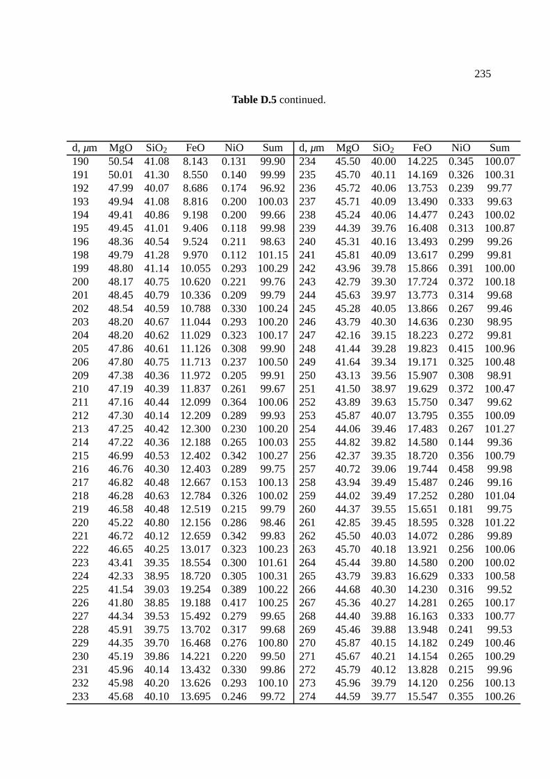
235
Table D.5continued.
d, µm MgO SiO2 FeO NiO Sum d, µm MgO SiO2 FeO NiO Sum190 50.54 41.08 8.143 0.131 99.90234 45.50 40.00 14.225 0.345 100.07191 50.01 41.30 8.550 0.140 99.99235 45.70 40.11 14.169 0.326 100.31192 47.99 40.07 8.686 0.174 96.92236 45.72 40.06 13.753 0.239 99.77193 49.94 41.08 8.816 0.200 100.03237 45.71 40.09 13.490 0.333 99.63194 49.41 40.86 9.198 0.200 99.66238 45.24 40.06 14.477 0.243 100.02195 49.45 41.01 9.406 0.118 99.98239 44.39 39.76 16.408 0.313 100.87196 48.36 40.54 9.524 0.211 98.63240 45.31 40.16 13.493 0.299 99.26198 49.79 41.28 9.970 0.112 101.15241 45.81 40.09 13.617 0.299 99.81199 48.80 41.14 10.055 0.293 100.29242 43.96 39.78 15.866 0.391 100.00200 48.17 40.75 10.620 0.221 99.76243 42.79 39.30 17.724 0.372 100.18201 48.45 40.79 10.336 0.209 99.79244 45.63 39.97 13.773 0.314 99.68202 48.54 40.59 10.788 0.330 100.24245 45.28 40.05 13.866 0.267 99.46203 48.20 40.67 11.044 0.293 100.20246 43.79 40.30 14.636 0.230 98.95204 48.20 40.62 11.029 0.323 100.17247 42.16 39.15 18.223 0.272 99.81205 47.86 40.61 11.126 0.308 99.90248 41.44 39.28 19.823 0.415 100.96206 47.80 40.75 11.713 0.237 100.50249 41.64 39.34 19.171 0.325 100.48209 47.38 40.36 11.972 0.205 99.91250 43.13 39.56 15.907 0.308 98.91210 47.19 40.39 11.837 0.261 99.67251 41.50 38.97 19.629 0.372 100.47211 47.16 40.44 12.099 0.364 100.06252 43.89 39.63 15.750 0.347 99.62212 47.30 40.14 12.209 0.289 99.93253 45.87 40.07 13.795 0.355 100.09213 47.25 40.42 12.300 0.230 100.20254 44.06 39.46 17.483 0.267 101.27214 47.22 40.36 12.188 0.265 100.03255 44.82 39.82 14.580 0.144 99.36215 46.99 40.53 12.402 0.342 100.27256 42.37 39.35 18.720 0.356 100.79216 46.76 40.30 12.403 0.289 99.75257 40.72 39.06 19.744 0.458 99.98217 46.82 40.48 12.667 0.153 100.13258 43.94 39.49 15.487 0.246 99.16218 46.28 40.63 12.784 0.326 100.02259 44.02 39.49 17.252 0.280 101.04219 46.58 40.48 12.519 0.215 99.79260 44.37 39.55 15.651 0.181 99.75220 45.22 40.80 12.156 0.286 98.46261 42.85 39.45 18.595 0.328 101.22221 46.72 40.12 12.659 0.342 99.83262 45.50 40.03 14.072 0.286 99.89222 46.65 40.25 13.017 0.323 100.23263 45.70 40.18 13.921 0.256 100.06223 43.41 39.35 18.554 0.300 101.61264 45.44 39.80 14.580 0.200 100.02224 42.33 38.95 18.720 0.305 100.31265 43.79 39.83 16.629 0.333 100.58225 41.54 39.03 19.254 0.389 100.22266 44.68 40.30 14.230 0.316 99.52226 41.80 38.85 19.188 0.417 100.25267 45.36 40.27 14.281 0.265 100.17227 44.34 39.53 15.492 0.279 99.65268 44.40 39.88 16.163 0.333 100.77228 45.91 39.75 13.702 0.317 99.68269 45.46 39.88 13.948 0.241 99.53229 44.35 39.70 16.468 0.276 100.80270 45.87 40.15 14.182 0.249 100.46230 45.19 39.86 14.221 0.220 99.50271 45.67 40.21 14.154 0.265 100.29231 45.96 40.14 13.432 0.330 99.86272 45.79 40.12 13.828 0.215 99.96232 45.98 40.20 13.626 0.293 100.10273 45.96 39.79 14.120 0.256 100.13233 45.68 40.10 13.695 0.246 99.72274 44.59 39.77 15.547 0.355 100.26

236 APPENDIX D. EXAMPLE PROFILE ANALYSES
Table D.5continued.
d, µm MgO SiO2 FeO NiO Sum d, µm MgO SiO2 FeO NiO Sum275 42.95 39.25 17.365 0.252 99.81316 45.25 39.47 14.759 0.326 99.80276 45.19 39.99 14.564 0.269 100.01317 42.93 39.27 18.828 0.342 101.37277 45.90 40.09 13.612 0.350 99.95318 41.14 39.01 20.306 0.355 100.82278 45.41 40.08 14.766 0.249 100.51319 40.60 38.99 20.141 0.295 100.03279 44.05 39.65 16.693 0.293 100.69320 40.92 38.88 20.714 0.386 100.90280 43.22 39.60 16.283 0.308 99.42321 41.67 39.04 18.901 0.325 99.93281 45.20 39.95 14.409 0.249 99.81322 45.44 39.90 14.236 0.304 99.88282 42.36 39.06 19.299 0.403 101.12323 45.70 40.13 13.947 0.232 100.01283 45.64 39.93 14.090 0.241 99.90324 45.55 39.87 13.939 0.300 99.66284 45.98 39.97 14.028 0.384 100.36325 42.01 38.87 20.063 0.411 101.35285 45.55 39.83 14.061 0.260 99.69326 43.44 39.33 16.454 0.337 99.57286 45.70 39.94 14.223 0.247 100.11327 44.78 39.76 15.653 0.304 100.50287 45.48 39.97 14.420 0.213 100.08328 44.37 39.67 15.116 0.322 99.48288 44.51 40.59 14.217 0.249 99.57329 45.73 39.86 14.181 0.214 99.99289 45.40 40.29 14.380 0.309 100.38330 40.82 38.74 20.566 0.442 100.56290 45.68 40.01 14.063 0.365 100.12331 40.70 38.84 20.808 0.377 100.72291 46.05 40.20 14.330 0.354 100.93332 40.21 38.67 20.628 0.364 99.87292 45.79 40.33 14.059 0.238 100.42333 40.19 38.69 20.397 0.333 99.62293 45.84 40.18 14.285 0.197 100.50334 41.13 39.09 19.741 0.277 100.24294 45.77 40.05 14.189 0.244 100.24335 44.30 40.06 15.004 0.294 99.66295 45.92 40.10 14.406 0.260 100.68336 45.54 40.08 14.163 0.272 100.06296 45.36 40.16 14.537 0.232 100.29337 45.85 39.90 13.979 0.276 100.00297 45.32 39.99 14.442 0.279 100.04338 45.54 39.96 14.361 0.216 100.08298 45.56 39.99 14.127 0.279 99.96339 45.20 39.83 14.865 0.248 100.15299 44.58 40.36 13.997 0.241 99.17340 41.98 39.06 19.975 0.462 101.47300 43.83 39.66 16.620 0.293 100.41341 40.58 39.03 20.034 0.419 100.06301 42.13 39.18 17.950 0.321 99.58342 40.28 38.93 20.103 0.281 99.59302 45.40 40.15 14.176 0.204 99.93343 41.62 38.44 15.321 0.319 95.70303 45.69 40.25 14.584 0.347 100.88344 45.81 39.79 14.483 0.285 100.36304 44.95 40.59 14.135 0.229 99.91345 45.81 39.98 14.248 0.330 100.37305 44.53 41.06 13.828 0.191 99.61346 45.50 39.85 13.828 0.295 99.48306 45.96 40.19 14.259 0.172 100.57347 45.73 39.93 14.122 0.239 100.02307 45.73 40.13 14.124 0.263 100.24348 45.68 40.03 13.996 0.257 99.96308 43.62 39.42 17.881 0.361 101.28349 45.53 39.81 14.270 0.274 99.88309 41.12 39.06 20.069 0.305 100.55350 45.63 39.77 14.257 0.280 99.93310 40.59 39.09 19.683 0.523 99.88351 45.89 39.93 14.433 0.336 100.58311 40.76 38.69 20.393 0.420 100.27352 45.44 39.99 13.951 0.289 99.66312 40.53 39.00 19.978 0.504 100.01353 45.33 40.03 14.328 0.323 100.00313 41.19 38.84 19.457 0.411 99.90354 44.85 39.77 14.203 0.358 99.18314 44.79 39.58 15.018 0.328 99.71355 44.23 39.73 14.687 0.330 98.98315 45.40 39.78 14.159 0.251 99.59356 43.99 39.45 15.660 0.235 99.34

237
Table D.5continued.
d, µm MgO SiO2 FeO NiO Sum357 42.45 39.36 17.689 0.241 99.74358 41.67 38.80 19.560 0.400 100.43359 42.70 38.80 18.807 0.397 100.71360 42.75 38.92 19.270 0.316 101.25361 41.21 38.89 19.889 0.440 100.43362 41.39 38.89 19.497 0.318 100.09363 41.24 39.29 20.429 0.325 101.28364 41.70 39.13 19.996 0.284 101.11365 44.20 39.50 16.897 0.317 100.92366 44.97 39.79 14.810 0.293 99.86367 45.07 39.94 14.400 0.387 99.79368 45.43 39.79 14.275 0.286 99.79369 45.53 39.85 13.993 0.265 99.64370 45.54 39.76 14.106 0.336 99.74371 45.59 39.74 14.276 0.305 99.91372 45.32 39.77 14.428 0.317 99.84373 44.80 39.28 14.846 0.342 99.27374 44.56 39.43 14.284 0.280 98.55375 45.49 40.40 14.434 0.336 100.66376 45.38 40.19 14.400 0.323 100.30377 45.65 40.09 14.400 0.280 100.42378 45.04 39.84 14.389 0.359 99.62379 45.15 40.05 14.419 0.229 99.86380 45.65 39.93 14.623 0.199 100.40381 45.40 40.11 14.250 0.286 100.05
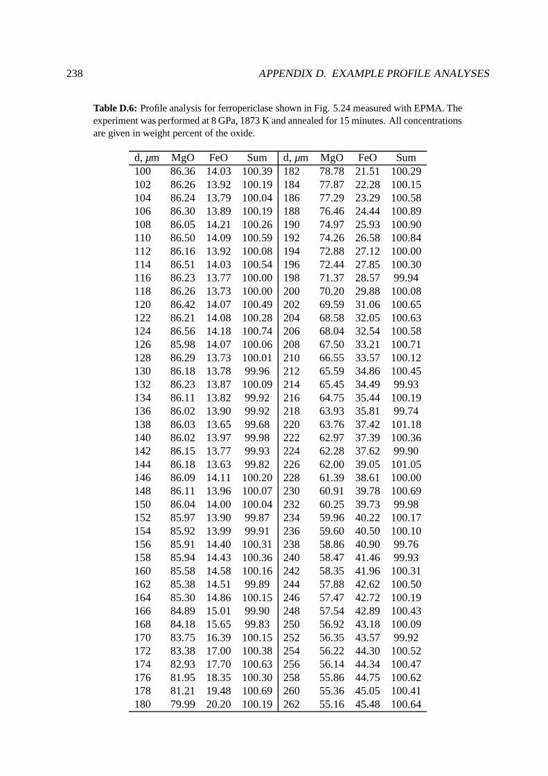
238 APPENDIX D. EXAMPLE PROFILE ANALYSES
Table D.6: Profile analysis for ferropericlase shown in Fig. 5.24 measured with EPMA. Theexperiment was performed at 8 GPa, 1873 K and annealed for 15 minutes. All concentrationsare given in weight percent of the oxide.
d, µm MgO FeO Sum d, µm MgO FeO Sum100 86.36 14.03 100.39182 78.78 21.51 100.29102 86.26 13.92 100.19184 77.87 22.28 100.15104 86.24 13.79 100.04186 77.29 23.29 100.58106 86.30 13.89 100.19188 76.46 24.44 100.89108 86.05 14.21 100.26190 74.97 25.93 100.90110 86.50 14.09 100.59192 74.26 26.58 100.84112 86.16 13.92 100.08194 72.88 27.12 100.00114 86.51 14.03 100.54196 72.44 27.85 100.30116 86.23 13.77 100.00198 71.37 28.57 99.94118 86.26 13.73 100.00200 70.20 29.88 100.08120 86.42 14.07 100.49202 69.59 31.06 100.65122 86.21 14.08 100.28204 68.58 32.05 100.63124 86.56 14.18 100.74206 68.04 32.54 100.58126 85.98 14.07 100.06208 67.50 33.21 100.71128 86.29 13.73 100.01210 66.55 33.57 100.12130 86.18 13.78 99.96 212 65.59 34.86 100.45132 86.23 13.87 100.09214 65.45 34.49 99.93134 86.11 13.82 99.92 216 64.75 35.44 100.19136 86.02 13.90 99.92 218 63.93 35.81 99.74138 86.03 13.65 99.68 220 63.76 37.42 101.18140 86.02 13.97 99.98 222 62.97 37.39 100.36142 86.15 13.77 99.93 224 62.28 37.62 99.90144 86.18 13.63 99.82 226 62.00 39.05 101.05146 86.09 14.11 100.20228 61.39 38.61 100.00148 86.11 13.96 100.07230 60.91 39.78 100.69150 86.04 14.00 100.04232 60.25 39.73 99.98152 85.97 13.90 99.87 234 59.96 40.22 100.17154 85.92 13.99 99.91 236 59.60 40.50 100.10156 85.91 14.40 100.31238 58.86 40.90 99.76158 85.94 14.43 100.36240 58.47 41.46 99.93160 85.58 14.58 100.16242 58.35 41.96 100.31162 85.38 14.51 99.89 244 57.88 42.62 100.50164 85.30 14.86 100.15246 57.47 42.72 100.19166 84.89 15.01 99.90 248 57.54 42.89 100.43168 84.18 15.65 99.83 250 56.92 43.18 100.09170 83.75 16.39 100.15252 56.35 43.57 99.92172 83.38 17.00 100.38254 56.22 44.30 100.52174 82.93 17.70 100.63256 56.14 44.34 100.47176 81.95 18.35 100.30258 55.86 44.75 100.62178 81.21 19.48 100.69260 55.36 45.05 100.41180 79.99 20.20 100.19262 55.16 45.48 100.64
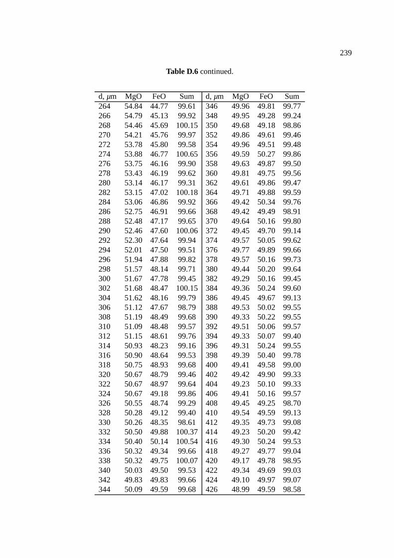
239
Table D.6continued.
d, µm MgO FeO Sum d, µm MgO FeO Sum264 54.84 44.77 99.61 346 49.96 49.81 99.77266 54.79 45.13 99.92 348 49.95 49.28 99.24268 54.46 45.69 100.15350 49.68 49.18 98.86270 54.21 45.76 99.97 352 49.86 49.61 99.46272 53.78 45.80 99.58 354 49.96 49.51 99.48274 53.88 46.77 100.65356 49.59 50.27 99.86276 53.75 46.16 99.90 358 49.63 49.87 99.50278 53.43 46.19 99.62 360 49.81 49.75 99.56280 53.14 46.17 99.31 362 49.61 49.86 99.47282 53.15 47.02 100.18364 49.71 49.88 99.59284 53.06 46.86 99.92 366 49.42 50.34 99.76286 52.75 46.91 99.66 368 49.42 49.49 98.91288 52.48 47.17 99.65 370 49.64 50.16 99.80290 52.46 47.60 100.06372 49.45 49.70 99.14292 52.30 47.64 99.94 374 49.57 50.05 99.62294 52.01 47.50 99.51 376 49.77 49.89 99.66296 51.94 47.88 99.82 378 49.57 50.16 99.73298 51.57 48.14 99.71 380 49.44 50.20 99.64300 51.67 47.78 99.45 382 49.29 50.16 99.45302 51.68 48.47 100.15384 49.36 50.24 99.60304 51.62 48.16 99.79 386 49.45 49.67 99.13306 51.12 47.67 98.79 388 49.53 50.02 99.55308 51.19 48.49 99.68 390 49.33 50.22 99.55310 51.09 48.48 99.57 392 49.51 50.06 99.57312 51.15 48.61 99.76 394 49.33 50.07 99.40314 50.93 48.23 99.16 396 49.31 50.24 99.55316 50.90 48.64 99.53 398 49.39 50.40 99.78318 50.75 48.93 99.68 400 49.41 49.58 99.00320 50.67 48.79 99.46 402 49.42 49.90 99.33322 50.67 48.97 99.64 404 49.23 50.10 99.33324 50.67 49.18 99.86 406 49.41 50.16 99.57326 50.55 48.74 99.29 408 49.45 49.25 98.70328 50.28 49.12 99.40 410 49.54 49.59 99.13330 50.26 48.35 98.61 412 49.35 49.73 99.08332 50.50 49.88 100.37414 49.23 50.20 99.42334 50.40 50.14 100.54416 49.30 50.24 99.53336 50.32 49.34 99.66 418 49.27 49.77 99.04338 50.32 49.75 100.07420 49.17 49.78 98.95340 50.03 49.50 99.53 422 49.34 49.69 99.03342 49.83 49.83 99.66 424 49.10 49.97 99.07344 50.09 49.59 99.68 426 48.99 49.59 98.58

240 APPENDIX D. EXAMPLE PROFILE ANALYSES
Table D.6continued.
d, µm MgO FeO Sum428 49.17 49.62 98.80430 49.30 50.23 99.54432 48.95 49.67 98.62434 49.19 49.99 99.18436 49.16 49.99 99.15438 49.41 50.21 99.62440 49.21 50.22 99.43

241
Table D.7: Profile analysis for ferropericlase shown in Fig. 5.25 measured with EPMA. Theexperiment was performed at 23 GPa, 1851 K and annealed for 183 minutes. All concentra-tions are given in weight percent of the oxide.
d, µm MgO FeO Sum d, µm MgO FeO Sum200 87.23 12.96 100.18118 55.82 45.67 101.48198 87.48 13.45 100.93116 55.19 46.08 101.27196 87.24 13.19 100.42114 55.00 46.48 101.48194 87.29 13.07 100.36112 54.55 46.89 101.44192 87.34 13.28 100.62110 53.98 47.05 101.02190 87.36 13.15 100.52108 53.66 47.14 100.80188 86.86 13.56 100.43106 53.53 47.37 100.90186 87.71 13.50 101.21104 53.04 47.86 100.90184 87.40 13.25 100.65102 52.92 47.84 100.76182 87.24 13.57 100.80100 52.71 48.67 101.39180 86.95 13.44 100.3998 52.30 48.92 101.23178 86.53 13.45 99.98 96 52.14 48.50 100.64176 86.43 13.97 100.4194 51.86 48.83 100.69174 85.48 14.46 99.94 92 51.59 49.15 100.74172 84.76 14.91 99.67 90 51.56 49.05 100.61170 84.07 15.82 99.89 88 51.35 49.69 101.03168 83.05 16.97 100.0286 51.33 49.40 100.73166 83.20 18.27 101.4784 51.16 49.49 100.65164 83.44 19.75 103.1982 51.06 49.87 100.92162 77.02 21.88 98.90 80 50.44 49.21 99.65160 77.66 23.72 101.3878 50.11 50.21 100.32158 76.32 24.90 101.2276 50.22 50.00 100.21156 74.81 26.37 101.1874 50.04 50.04 100.08154 73.30 28.06 101.3672 50.38 49.89 100.26152 71.36 29.40 100.7670 50.51 50.27 100.78150 69.72 31.23 100.9568 50.43 50.44 100.87148 68.48 32.96 101.4366 50.52 50.63 101.15146 66.64 34.40 101.0464 50.47 50.84 101.31144 65.45 35.71 101.1662 50.29 50.87 101.16142 64.40 36.75 101.1560 50.31 50.56 100.86140 63.22 38.23 101.4558 50.28 51.13 101.41138 62.37 38.57 100.9456 50.30 50.58 100.88136 61.60 39.84 101.4554 50.23 51.06 101.29134 60.90 39.99 100.8852 50.26 50.32 100.58132 59.98 41.46 101.4450 50.25 51.11 101.35130 59.45 41.59 101.0448 50.16 50.50 100.66128 58.31 42.33 100.6446 49.95 51.01 100.96126 57.20 43.26 100.4644 50.30 51.34 101.64124 57.04 44.13 101.1742 50.00 51.09 101.08122 56.39 44.69 101.0840 50.30 51.16 101.45120 56.07 44.94 101.0138 50.02 50.54 100.56

242 APPENDIX D. EXAMPLE PROFILE ANALYSES
Table D.7continued.
d, µm MgO FeO Sum38 50.02 50.54 100.5636 49.99 50.27 100.2534 50.28 51.42 101.7032 50.46 51.15 101.6130 49.85 50.80 100.6528 50.24 51.16 101.4126 50.20 51.22 101.4324 50.22 50.80 101.0222 50.10 50.76 100.8620 50.09 51.05 101.14

243
Table D.8: Profile analysis for ferropericlase shown in Fig. 5.26 measured with EPMA. Theexperiment was performed at 8 GPa, 1873 K and annealed for 20 minutes. All concentrationsare given in weight percent of the oxide.
d, µm MgO FeO Sum d, µm MgO FeO Sum380 98.25 0.14 98.39 328 67.32 32.12 99.45379 98.13 0.13 98.27 327 66.99 32.94 99.93375 97.99 0.21 98.20 326 66.51 32.98 99.49374 98.42 0.20 98.62 325 66.21 33.45 99.66372 98.23 0.21 98.44 324 65.40 33.75 99.14371 98.53 0.25 98.78 323 64.61 33.50 98.11370 98.41 0.23 98.64 322 64.87 34.56 99.43369 98.31 0.29 98.60 321 64.81 35.55 100.36367 97.83 0.27 98.11 320 64.21 35.60 99.81366 97.84 0.23 98.07 319 63.69 35.88 99.57360 98.17 0.56 98.73 318 63.36 36.41 99.78359 97.64 0.90 98.53 317 62.80 36.54 99.34358 97.38 1.74 99.12 316 62.84 37.25 100.08357 96.03 2.54 98.57 315 62.17 37.70 99.86356 95.19 3.73 98.92 314 61.76 37.92 99.68355 93.74 5.33 99.06 313 61.50 38.02 99.52354 91.97 7.14 99.11 312 61.21 38.71 99.91353 89.27 8.82 98.09 311 60.90 39.15 100.05351 87.26 11.89 99.15 310 60.27 39.05 99.31350 86.23 13.38 99.61 309 60.52 39.59 100.11349 85.01 14.55 99.56 308 60.08 39.85 99.93348 83.88 16.30 100.17307 59.81 40.14 99.95347 82.43 17.29 99.72 306 59.43 40.50 99.93346 81.46 18.14 99.59 305 59.24 40.63 99.87345 80.69 18.81 99.50 304 59.15 40.74 99.88344 79.72 19.79 99.51 303 59.00 41.08 100.09343 78.97 20.76 99.73 302 58.59 40.65 99.24342 78.02 21.74 99.76 301 58.13 41.29 99.42341 76.82 22.85 99.68 300 58.38 41.51 99.89340 76.25 23.43 99.68 299 57.61 41.49 99.10339 75.27 24.42 99.69 298 57.97 42.02 99.99338 74.42 25.45 99.87 297 57.61 42.06 99.67337 73.74 26.33 100.06296 57.60 42.11 99.71336 72.71 26.38 99.09 295 57.32 42.72 100.05335 71.32 27.08 98.40 294 56.89 42.66 99.55334 71.20 28.32 99.52 293 56.67 43.34 100.01333 70.43 29.01 99.44 292 56.34 42.71 99.06332 69.72 29.92 99.64 291 56.66 43.39 100.06331 69.26 30.50 99.75 290 56.18 43.47 99.65330 68.72 31.53 100.25289 55.93 43.69 99.62329 67.85 31.89 99.74 288 55.77 43.64 99.40

244 APPENDIX D. EXAMPLE PROFILE ANALYSES
Table D.8continued.
d, µm MgO FeO Sum d, µm MgO FeO Sum286 55.51 43.91 99.43 241 51.64 47.70 99.34285 55.34 43.89 99.23 240 51.87 47.88 99.74284 55.34 44.29 99.63 239 51.35 47.84 99.20283 55.20 44.45 99.65 238 51.65 47.56 99.22282 55.06 44.82 99.88 237 51.49 47.81 99.30281 55.12 44.60 99.72 236 51.63 47.96 99.59280 54.55 45.04 99.59 235 51.47 48.18 99.64279 54.86 44.90 99.76 234 51.59 47.88 99.47278 54.48 44.79 99.28 233 51.39 48.18 99.58277 54.15 45.07 99.21 232 51.30 48.13 99.43276 54.25 45.28 99.53 231 51.39 48.46 99.84275 54.16 45.27 99.43 230 51.10 47.75 98.84274 54.08 45.23 99.32 229 50.56 46.97 97.54273 53.44 45.47 98.91 228 51.08 48.40 99.48272 53.83 45.79 99.62 227 50.98 48.02 99.00271 53.33 45.68 99.01 226 51.08 48.21 99.29270 53.22 46.13 99.35 225 51.06 48.40 99.45266 53.41 46.18 99.59 224 50.91 48.32 99.23265 53.28 46.33 99.61 223 51.03 48.20 99.23264 53.03 46.32 99.35 222 50.78 48.54 99.32263 52.84 46.10 98.94 221 51.30 48.06 99.36262 52.89 46.43 99.32 220 50.82 48.72 99.54261 52.47 45.96 98.43 219 50.88 48.40 99.28260 52.70 46.21 98.91 218 51.02 48.49 99.51259 52.89 47.05 99.94 217 50.98 48.82 99.80258 52.65 46.63 99.28 216 51.07 48.77 99.84257 52.96 46.83 99.80 215 50.91 48.74 99.65256 52.59 47.02 99.60 214 50.88 48.64 99.52255 51.66 46.82 98.47 213 50.88 48.65 99.53254 51.99 46.86 98.86 212 50.77 48.90 99.67253 52.07 47.04 99.11 211 50.76 48.68 99.44252 52.29 47.13 99.42 210 51.03 48.54 99.57251 52.20 47.24 99.44 209 50.78 49.02 99.80250 52.24 47.64 99.88 208 50.99 48.85 99.83249 52.04 47.53 99.56 207 50.95 49.13 100.08248 52.36 47.34 99.70 206 50.62 48.96 99.58247 51.97 47.46 99.43 205 50.77 48.78 99.55246 51.96 47.67 99.63 204 50.66 48.93 99.60245 51.68 47.57 99.25 203 50.56 48.82 99.38244 51.92 47.37 99.28 202 50.51 48.38 98.89243 51.76 47.94 99.71 201 50.86 49.36 100.22242 51.81 48.30 100.11200 50.74 48.85 99.59241 51.64 47.70 99.34

245
Table D.9: Profile analysis for perovskite shown in Fig. 5.36 measured with EDX-STEM.The experiment was performed at 25 GPa, 2023 K and annealed for 483 minutes.XFeSiO3
denotes mole fraction of FeSiO3 in (Mg,Fe)SiO3 perovskite. MgO loss was corrected asdiscussed in Section 5.5.4
d, µm XFeSiO3
0.105 0.0450.132 0.0470.158 0.0470.184 0.0510.211 0.0470.237 0.0490.263 0.0430.289 0.0370.316 0.0260.342 0.0150.368 0.0120.395 0.0060.421 0.0040.447 0.0020.474 0.0020.500 0.003
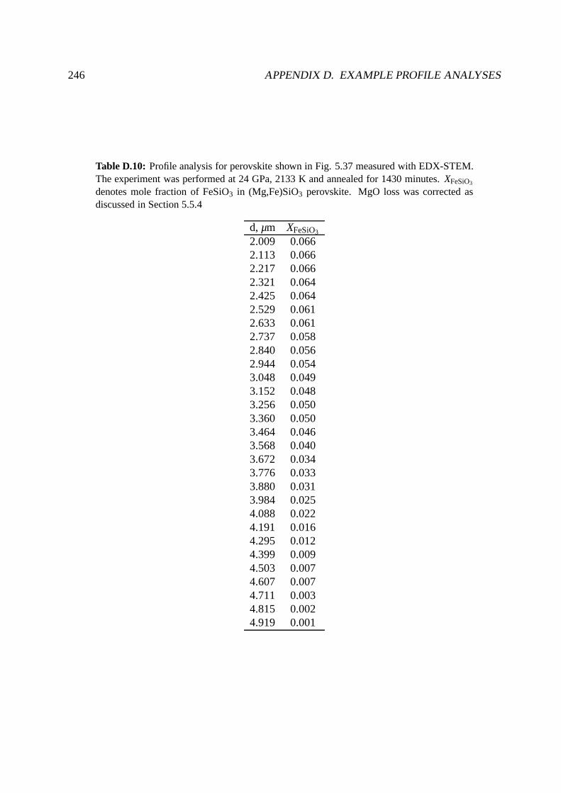
246 APPENDIX D. EXAMPLE PROFILE ANALYSES
Table D.10: Profile analysis for perovskite shown in Fig. 5.37 measured with EDX-STEM.The experiment was performed at 24 GPa, 2133 K and annealed for 1430 minutes.XFeSiO3
denotes mole fraction of FeSiO3 in (Mg,Fe)SiO3 perovskite. MgO loss was corrected asdiscussed in Section 5.5.4
d, µm XFeSiO3
2.009 0.0662.113 0.0662.217 0.0662.321 0.0642.425 0.0642.529 0.0612.633 0.0612.737 0.0582.840 0.0562.944 0.0543.048 0.0493.152 0.0483.256 0.0503.360 0.0503.464 0.0463.568 0.0403.672 0.0343.776 0.0333.880 0.0313.984 0.0254.088 0.0224.191 0.0164.295 0.0124.399 0.0094.503 0.0074.607 0.0074.711 0.0034.815 0.0024.919 0.001

247
Table D.11: Profile analyses for perovskite shown in Fig. 5.39 measured with EDX-STEM.The experiment was performed at 26 GPa, 1973 K and annealed for 570 minutes.XFeSiO3
denotes mole fraction of FeSiO3 in (Mg,Fe)SiO3 perovskite. MgO loss was corrected asdiscussed in Section 5.5.4
d, µm XFeSiO3 d, µm XFeSiO3 d, µm XFeSiO3
0.0 0.107 1.6 0.103 0.0 0.1070.2 0.113 1.7 0.079 0.1 0.1080.4 0.112 1.8 0.060 0.2 0.1060.6 0.115 1.9 0.043 0.3 0.1070.8 0.114 2.0 0.034 0.4 0.1051.0 0.114 2.1 0.020 0.5 0.1041.2 0.114 0.6 0.1031.4 0.112 0.7 0.1011.6 0.113 0.8 0.1021.8 0.111 0.9 0.0982.0 0.111 1.0 0.0972.2 0.106 1.1 0.1002.4 0.091 1.2 0.0982.6 0.040 1.3 0.0962.8 0.018 1.4 0.0853.0 0.010 1.5 0.0593.2 0.006 1.6 0.0363.4 0.001 1.7 0.0243.6 0.001 1.8 0.0183.8 0.001 1.9 0.0144.0 0.001 2.0 0.0124.2 0.001 2.1 0.0114.4 0.002 2.2 0.0094.6 0.002 2.3 0.0084.8 0.002 2.4 0.0075.0 0.002 2.5 0.006
2.6 0.0062.7 0.0052.8 0.0042.9 0.0043.0 0.004

248 APPENDIX D. EXAMPLE PROFILE ANALYSES

Appendix E
Example EDX-spectra of silicate perovskite
The example spectra are taken from sample C23, annealed at 24GPa, 2123 K for 720 min. In
Figure E.1 a spectrum of MgSiO3 perovskite and in E.2 a spectrum of (Mg,Fe)SiO3 perovskite
is shown. The Mo peak appears because scatterd electrons produce X-ray emission from the
Mo grid. In case of Cu grids, instead of Mo, Cu peaks are observed. Hence, in the Vantage
software the Mo or Cu peak were considered for determinationof the intensities (software op-
tion ”present”) but the intensities of Cu and Mo were than notused for the calculation of the
absorption corrected concentrations. The relative intensity of the Mg peak especially on the Fe-
poor side of the diffusion interface indicates Mg loss during the analysis (see Section 5.5.4 for
further details). In all analysis performed in this study, spectra were recorded for a lifetime of 60
seconds. The dead time was usually between 15 and 30%.
249

25
0A
PP
EN
DIX
E.
EX
AM
PLE
ED
X-S
PE
CT
RA
OF
SIL
ICAT
EP
ER
OV
SK
ITE
0
500
1000
1500
2000
2500
3000
1 2 3 4 5 6 7 8
Cou
nts
Energy, keV
Si
Mg
O
FeKα Kβ
Mo
dead time
18%
Figure E.1: Example EDX spectrum of an Fe-poor perovskite.
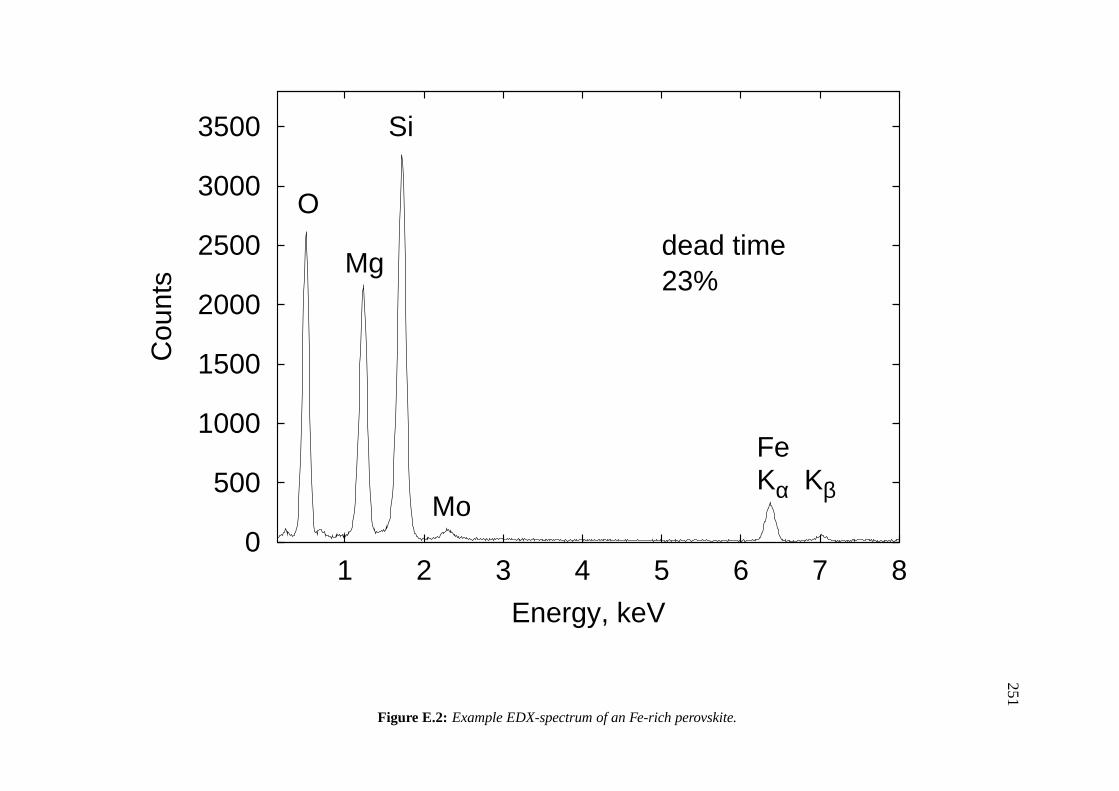
25
1
0
500
1000
1500
2000
2500
3000
3500
1 2 3 4 5 6 7 8
Cou
nts
Energy, keV
Si
Mg
O
FeKα Kβ
Mo
dead time23%
Figure E.2: Example EDX-spectrum of an Fe-rich perovskite.

252 APPENDIX E. EXAMPLE EDX-SPECTRA OF SILICATE PEROVSKITE
Bibliography
Akaogi, M. and Akimoto, S. (1977). Pyroxene-garnet solid solution equilibria in the systems
Mg4Si4O12-Mg3Al2Si3O12 and Fe4Si4O12-Fe3Al2Si3O12 at high pressures and temperatures.
Physics of The Earth and Planetary Interiors, 15: 90–106.
Akaogi, M., Ito, E., and Navrotsky, A. (1989). Olivine-modified spinel-spinel transitions in
the system Mg2SiO4-Fe2SiO4: Calorimetric measurements, thermochemical calculationand
geophysical application.Journal of Geophysical Research, 94: 15671–15685.
Akaogi, M., Ross, N., McMillan, P., and Navrotsky, A. (1984). The Mg2SiO4 polymorphs
(olivine, modified spinel and spinel) - thermodynamic properties from oxide melt solution
calorimetry, phase relations and models of lattice vibrations.American Mineralogist, 69: 499–
512.
Allnatt, A. R. and Lidiard, A. B. (1993).Atomic transport in solids. Cambridge University Press,
Cambridge.
Anderson, O. L. (1982). The Earth’s core and the phase diagram of iron. Philosophical Trans-
actions of the Royal Society of London, A306: 21–35.
Appel, M. and Pask, J. A. (1971). Interdiffusion and moving boundaries in NiO-CaO and NiO-
MgO single-crystal couples.Journal of the American Ceramic Society, 54: 152–58.
Badro, J., Fiquet, G., Guyot, F., Rueff, J.-P., Struzhkin, V. V., Vanko, G., and Monaco, G.
(2003). Iron partitioning in Earth’s mantle: Toward a deep lower mantle discontinuity.Science,
300: 789–791.
Bardeen, J. and Herring, C. (1952).Imperfections in Nearly Perfect Crystals. Wiley, New York.
253

254 BIBLIOGRAPHY
Barrer, R., Bartholomew, R., and Rees, L. (1963). Ion exchange in porous crystals. Part II -
the relationship between self- and exchange-diffusion coefficients. Journal of Physics and
Chemistry of Solids, 24: 309–317.
Bejina, F. (1999). Activation volume of Si diffusion in SanCarlos olivine: Implications for upper
mantle rheology.Journal of Geophysical Research, 104(B11): 25529–25542.
Bejina, F., Jaoul, O., and Liebermann, R. C. (2003). Diffusion in minerals at high pressure: A
review. Physics of the Earth and Planetary Interiors, 139: 3–20.
Blank, S. L. and Pask, J. A. (1969). Diffusion of iron and nickel in magnesium oxide single
crystals.Journal of the American Ceramic Society, 52: 669–675.
Bocquet, J. L., Brbec, G., and Limoge, Y. (1983). Diffusion in metals and alloys. In Cahn, R. W.
and Haasen, P., editors,Physical Metallurgy. Elsevier Science Publishers.
Boehler, R. (1996). Melting of mantle and core materials at very high pressures.Philosophical
Transactions of the Royal Society of London, 354: 1265–1278.
Bolfan-Casanova, N., Keppler, H., and Rubie, D. (2000). Water partitioning between nominally
anhydrous minerals in the MgO-SiO2-H2O system up to 24 GPa: Implications for the distibu-
tion of water in the Earth’s mantle.Earth and Planetary Science Letters, 182: 209–221.
Bolfan-Casanova, N., Mackwell, S., Keppler, H., McCammon,C., and Rubie, D. (2002). Pres-
sure dependence of H solubility in magnesiowustite up to 25GPa: Implications for the storage
of water in the Earth’s lower mantle.Geophysical Research Letters, 29: 89 – 1–4.
Brady, J. (1995). Diffusion data for silicate minerals, glasses, and liquids. In Ahrens, T., editor,
Mineral Physics & Crystallography - A Handbook of Physical Constants, volume 2 ofAGU
Reference Shelf, pages 269–290. American Geophysical Union, Washington.
Brady, J. B. (1975a). Chemical components and diffusion.American Journal of Science,
275: 1073–1088.
Brady, J. B. (1975b). Reference frames and diffusion coefficients.American Journal of Science,
275: 954–983.

BIBLIOGRAPHY 255
Buening, D. K. and Buseck, P. R. (1973). Fe-Mg lattice diffusion in olivine. Journal of Geo-
physical Research, 78: 6852–6862.
Bygden, J., Jakobsson, A., Sichen, D., and Seetharaman, S.(1997). Interdiffusion studies in the
system MgO-FeO.Zeitschrift fur Metallkunde, 88: 433–437.
Carslaw, H. S. and Jaeger, J. C. (1946).Conduction of Heat in Solids. Oxford University Press,
Oxford.
Chakraborty, S. (1995). Diffusion in silicate melts. In Stebbins, J. F., McMillan, P. F., and
Dingwell, D. B., editors,Structure, Dynamics and Properties of Silicate Melts, volume 32 of
Reviews in Mineralogy, pages 411 – 503. Mineralogical Society of America, Washington.
Chakraborty, S. (1997). Rates and mechanisms of Fe-Mg interdiffusion in olivine at 980◦c-
1300◦c. Journal of Geophysical Research, 102(B6): 12317–12331.
Chakraborty, S., Farver, J. R., Yund, R. A., and Rubie, D. C. (1994). Mg tracer diffusion in
synthetic forsterite and San Carlos olivine as a function ofP, T and fO2.Physics and Chemistry
of Minerals, 21: 489–500.
Chakraborty, S. and Ganguly, J. (1991). Compositional zoning and cation diffusion in garnets.
In Ganguly, J., editor,Diffusion, Atomic Ordering and Mass Transport: Selected Topics in
Geochemistry, volume 8 ofAdvances in Physical Geochemistry, pages 120–175. Springer,
New York.
Chakraborty, S. and Ganguly, J. (1992). Cation diffusion inaluminosilicate garnets: experimen-
tal determination in spessartine-almandine diffusion couples, evaluation of effective binary
diffusion coefficients, and applications.Contributions to Mineralogy and Petrology, 111: 74–
86.
Chakraborty, S., Knoche, R., Schulze, H., Rubie, D. C., Dobson, D., Ross, N. L., and Angel,
R. J. (1999). Enhancement of cation diffusion rates across the 410-kilometer discontinuity in
Earth’s mantle.Science, 283: 362–365.

256 BIBLIOGRAPHY
Chen, W. K. and Peterson, N. L. (1980). Iron diffusion and electrical conductivity in magne-
siowustite solid solutions (Mg,Fe)O.Journal of Physics and Chemistry of Solids, 41: 335–339.
Chudinovskikh, L. and Boehler, R. (2001). High-pressure polymorphs of olivine and the 660-km
seismic discontinuity.Nature, 411(6837): 574–577.
Clark, A. and Long, J. (1971). The anisotropic diffusion of nickel in olivine. In Sherwood, J.,
Chadwick, A., Muir, W., and Swinton, F., editors,Diffusion processes, pages 511–521. Gordon
and Breach, London.
Cottrell, E., Spiegelman, M., and Langmuir, C. H. (2002). Consequences of diffusive reequilibra-
tion for the interpretation of melt inclusions.Geochemistry Geophysics Geosystems, 3(5): U1–
U26.
Crank, J. (1979).The Mathematics of Diffusion. Oxford University Press, Oxford.
Darken, L. (1948). Diffusion, mobility and their interrelation through free energy in binary
metallic systems.Am. Inst. Mining Metall Engineers Trans., 175: 184–201.
Deer, W. A., Howie, R. A., and Zussman, J. (1992).An Introduction to the Rock-Forming Min-
erals. Longman Scientific & Technical, Harlow.
Denbigh, K. (1981). The Principles of Chemical Equilibrium. Cambridge University Press,
Cambridge.
Dubrovinsky, L. S., Dubrovinskaia, N., Annersten, H., Halenius, E., and Harryson, H. (2000a).
Stability of (Mg0.5Fe0.5)O and(Mg0.8Fe0.2)O magnesiowustites in the lower mantle.Euro-
pean Journal of Mineralogy, 13: 857–861.
Dubrovinsky, L. S., Dubrovinskaia, N., Saxena, S. K., Annersten, H., Halenius, E., Harryson, H.,
Tutti, F., Rekhi, S., and Le Bihan, T. (2000b). Stability of ferropericlase in the lower mantle.
Science, 289(5478): 430–432.
Dubrovinsky, L. S., Saxena, S. K., and Lazor, P. (1998). High-pressure and high-temperature in
situ X-ray diffraction study of iron and corundum to 68 GPa using internally heated diamond
anvil cell. Physics and Chemistry of Minerals, 25: 434–441.

BIBLIOGRAPHY 257
Duffy, T. S., Hemley, R. J., and Mao, H. K. (1995). Equation ofstate and shear strength at
multimegabar pressures: Magnesium oxide to 227 GPa.Physical Review Letters, 74: 1371–
1374.
Dziewonski, A. M. and Anderson, D. L. (1981). Preliminary reference Earth model.Physics of
the Earth and Planetary Interiors, 25: 297–356.
Edington, J. W. (1976).The Operation and Calibration of the Electron Microscope, volume 1 of
Monographs in practical electron microscopy in materials science, Philips technical library.
MacMillan.
Einstein, A. (1905). Eine neue Bestimmung der Molekudimension. Annalen der Physik, page
549.
Eremets, M. (1996).High Pressure Experimental Methods. Oxford University Press.
Farber, D. L., Williams, Q., and Ryerson, F. J. (2000). Divalent cation diffusion in Mg2SiO4
spinel (ringwoodite),β phase (wadsleyite), and olivine: Implications for the electrical conduc-
tivity of the mantle.Journal of Geophysical Research, 105(1): 513–529.
Fick, A. (1855).Uber Diffusion.Poggendorff ’s Annalen der Physik und Chemie, 94: 59–86.
Finger, L., Hazen, R., Zhang, J., Ko, J., and Navrotsky, A. (1993). The effect of Fe on the crystal
structure of wadsleyiteβ− (Mg1−xFex)2SiO4, 0.00≤ x ≤ 0.40. Physics and Chemistry of
Minerals, 19: 361–368.
Freer, R. (1980). Bibliography: self diffusion and impurity diffusion in oxides. Journal of
Materials Science, 15: 803–824.
Frost, B. (1991). Introduction to oxygen fugacity and its petrologic importance. In Lindsley,
D., editor,Oxide Minerals: Petrologic and Magnetic Significance, volume 25 ofReviews in
Mineralogy. Mineralogical Society of America, Washington, D.C.
Frost, D., Poe, B., Trønnes, R., Liebske, C., Duba, A., and Rubie, D. (2003). A new large-volume
multianvil system.Physics of the Earth and Planetary Interiors, submitted.

258 BIBLIOGRAPHY
Frost, D. J. and Langenhorst, F. (2002). The effect of Al2O3 on Fe-Mg partitioning between
magnesiowustite and magnesium silicate perovskite.Earth and Planetary Science Letters,
199: 227–241.
Gaetani, G. A. and Watson, E. B. (2002). Modeling the major-element evolution of olivine-
hosted melt inclusions.Chemical Geology, 183(1-4): 25–41.
Ganguly, J. (2002). Diffusion kinetics in minerals: Principles and applications to tectono-
metamorphic processes.EMU Notes in Mineralogy, 4: 271–309.
Ganguly, J., Bhattacharya, R. N., and Chakraborty, S. (1988). Convolution effect in the determi-
nation of compositional profiles and diffusion coefficientsby microprobe step scans.American
Mineralogist, 73: 901–909.
Gessmann, C. K. and Rubie, D. C. (2000). The origin of the depletions of V, Cr and Mn in the
mantles of the Earth and Moon.Earth and Planetary Science Letters, 184: 95–107.
Getting, I. C. and Kennedy, G. C. (1970). Effect of pressue onthe emf of chromel-alumel and
platinum-platinum 10% rhodium thermocouples.Journal of Applied Physics, 41(11): 4552–
4562.
Ghez, R. (1988).A Primer of Diffusion Problems. Joh Wiley & Sons, Inc.
Graham (1987). The multianvil press. In Sammis, C. G. and Henyey, T. L., editors,Geophysics
Part A, Laboratory Measurements, Methods of experimental physics. Academic Press, Or-
lando.
Harrison, L. (1961).Trans. Faraday Soc., 57: 1191.
Hashin, Z. and Shtrikman, S. (1962). A variational approachto the theory of the effective mag-
netic permeability of multiphase materials.Journal of Applied Physics, 33: 3125–3131.
Haussuhl, S. (1983).Kristallphysik. Physik Verlag, Verlag Chemie.
Heinrich, K. F. J. and Newbury, D. E. (1991).Electron Probe Quantification. Plenum Press,
New York and London.
BIBLIOGRAPHY 259
Hermeling, J. and Schmalzried, H. (1984). Tracerdiffusionof the Fe-cations in olivine
(FexMg1−x)2SiO4 (III). Physics and Chemistry of Minerals, 11: 161–166.
Herzberg, C. and Zhang, J. (1996). Melting experiments on anhydrous peridotite KLB-1: Com-
positions of magmas in the upper mantle and transition zone.Journal of Geophysical Re-
search, 101(B4): 8271–8295.
Herzig, C. and Mishin, Y. (1998). Grain boundary diffusion in metals. In Karger, J., Heitjyans,
P., and Haberland, R., editors,Diffusion in Condensed Matter, pages 90–115. Vieweg u. Sohn
Verlag.
Hofmann, A. W. (1997). Mantle geochemistry: the message from oceanic volcanism.Nature,
385: 219–229.
Holzapfel, C., Rubie, D., Mackwell, S., and Frost, D. (2003). Effect of pressure on Fe-Mg
interdiffusion in (FexMg1−x)O, ferropericlase.Physics of the Earth and Planetary Interiors,
139: 21–34.
Holzheid (1996).Aktivitaten von Metalloxiden geochemisch relevanter Elemente in silikatischen
Schmelzen und deren Implikationen fur die Kernbildung der Erde. PhD thesis, University of
Cologne.
Huebner, J. S. (1971). Buffering techniques for hydrostatic systems at elevated pressures. In
Ulmer, G., editor,Research Techniques for High Pressure and High Temperature, pages 146–
177. Springer.
Irifune, T. (1993). Phase transformations in the Earth’s mantle and subducting slabs; Implications
for their compositions, seismic velocity and density structures and dynamics.Island Arc,
2: 55–71.
Irifune, T. (1994). Absence of an aluminous phase in the upper part of the Earth’s lower mantle.
Nature, 370: 121–123.
Irifune, T. (2002). Application of synchrotron radiation and Kawai-type apparatus to various
studies in high-pressure mineral physics.Mineralogical Magazine, 66(5): 769–790.

260 BIBLIOGRAPHY
Irifune, T., Naka, H., Sanehira, T., Inoue, T., and Funakoshi, K. (2002). In situ X-ray observations
of phase transitions in MgAl2O4 spinel to 40 GPa using multianvil apparatus with sintered
diamond anvils.Physics and Chemistry of Minerals, 29: 645–654.
Irifune, T., Nishiyama, N., Kuroda, K., Inoue, T., Isshiki,M., Utsumi, W., Funakoshi, K.,
Urakawa, S., Uchida, T., Katsura, T., and Ohtaka, O. (1998).The postspinel phase bound-
ary in Mg2SiO4 determined by in situ X-ray diffraction.Science, 279: 1693–1700.
Ita, J. and Cohen, R. E. (1997). Effects of pressure on diffusion and vacancy formation in MgO
from nonempirical free-energy integrations.Physical Review Letters, 79: 3198–3201.
Ita, J. and Cohen, R. E. (1998). Diffusion in MgO at high pressure: Implications for lower mantle
rheology.Geophysical Reserach Letters, 25: 1095–1098.
Ito, M. and Takahashi, E. (1989). Post-spinel transformations in the system Mg2SiO4-Fe2SiO4
and some geophysical implications.Journal of Geophysical Research, 94: 10637–10646.
Ito, M., Yurimoto, H., Morioka, M., and Nagasawa, H. (1999).Co2+ and ni2+ diffusion in
olivine determined by secondary ion mass spectrometry.Physics and Chemistry of Minerals,
26: 425–431.
Jackson, I. and Rigden, S. M. (1998). Composition and temperature of the Earth’s mantle:
Seismological models interpreted through experimental studies of Earth materials. In Jackson,
I., editor,The Earth’s Mantle: Composition, Structure, and Evolution, page 566. Cambridge
University Press, Cambridge.
Jakobsson, A. (1996). Diffusion studies in the system NiO-MgO using high temperature X-ray
technique.Zeitschrift fur Metallkunde, 87: 55–60.
Jaoul, O., Bertran-Alvarez, Y., Liebermann, R. C., and Price, G. D. (1995). Fe-Mg interdiffu-
sion in olivine up to 9 GPa at T = 600-900◦C; experimental data and comparison with defect
calulations.Physics of the Earth and Planetary Interiors, 89: 199–218.
Jeanloz, R. and Thompson, A. B. (1983). Phase transitions and mantle discontinuities.Rev.
Geophys. Space Phys., 21: 51–74.

BIBLIOGRAPHY 261
Jost, W. and Hauffe, K. (1972).Diffusion - Methoden der Messung und Auswertung, volume 1
of Fortschritte der physikalischen Chemie. Dr. Dietrich Steinkopff Verlag, Darmstadt.
Jurewicz, A. J. G. and Watson, E. B. (1988). Diffusion in olivine xenocrysts, with applications
to petrology and mineral physics.Contributions to Mineralogy and Petrology, 99: 186–201.
Karato, S.-I. (1981). Rheology of the lower mantle.Physics of the Earth and Planetary Interiors,
24: 1–14.
Karato, S.-I. and Murthy, V. R. (1997). Core formation and chemical equilibrium in the Earth -
I. Physical considerations.Physics of the Earth and Planetary Interiors, 100: 61–79.
Kato, T. and Kumazawa, M. (1985). Effect of high-pressure onthe melting relation in the system
Mg2SiO4-MgSiO3. J Phys Earth, 33: 513–524.
Katsura, T. and Ito, E. (1989). The system Mg2SiO4-Fe2SiO4 at high pressures and tempera-
tures: Precise determination of stabilities of olivine, modified spinel, and spinel.Journal of
Geophysical Research, 94(B11): 15663–15670.
Katsura, T., Yamada, H., Shinmei, T., Kubo, A., Ono, S., Kanzaki, M., Yoneda, A., Walter, M.,
Ito, E., Urakawa, S., Funakoshi, K., and Utsumi, W. (2003). Post-spinel transition in Mg2SiO4
determined by high P-T in situ X-ray diffractometry.Physics of the Earth and Planetary
Interiors, 136: 11–24.
Kawai, N. and Endo, S. (1970). The generation of ultrahigh hydrostatic pressures by a split
sphere apparatus.Review of Scientific Instruments, 41: 1178–1181.
Kawai, N., Togaya, M., and Onodera, A. (1973).Proc. Jpn Acad., 49: 623–626.
Kleine, T., Munker, C., Mezger, K., and Palme, H. (2002). Rapid accretion and early core
formation on asteroids and the terrestrial planets from Hf-W chronometry.Nature, 418: 952–
955.
Kohlstedt, D. L., Keppler, H., and Rubie, D. C. (1996). Solubility of water in theα, β, andγ
phases of (Mg,Fe)2SiO4. Contrib. Mineral. Petrol., 123: 345–357.

262 BIBLIOGRAPHY
Langenhorst, F. (1995). Thermal and shock metamorphism of the Tenham chondrite: A TEM
examination.Geochimica et Cosmochimica Acta, 59(9): 1835–1845.
Lauterbach, S. (2000).Der Oxidationsgrad des Eisens im unteren Mantel: Eine Studie des
Fe3+-Gehaltes des Silikat-Perowskits in Abhangigkeit seines Al-Gehaltes mit Mossbauer-
Spektroskopie und Elektronen-Energie-Verlust-Spektroskopie (EELS). phd, Universitat
Bayreuth.
Lauterbach, S., McCammon, C. A., van Aken, P., Langenhorst,F., and Seifert, F. (2000).
Mossbauer and ELNES spectroscopy of (Mg,Fe)(Si,Al)O3 perovskite: A highly oxidised com-
ponent of the lower mantle.Contributions to Mineralogy and Petrology, 138(1): 17–26.
Li, J. and Agee, C. B. (1996). Geochemistry of mantle-core formation at high pressure.Nature,
381: 686–689.
Li, J. and Agee, C. B. (2001). The effect of pressure, temperature, oxygen fugacity and com-
position on partitioning of nickel and cobalt between liquid Fe-Ni-S alloy and liquid silicate:
Implications for the Earth’s core formation.Geochimica et Cosmochimica Acta, 65(11): 1821–
1832.
Liebermann, R. C. and Wang, Y. (1992). Characterization of sample environment in a uniaxial
split-sphere apparatus. In Syono, Y. and Manghnani, M. H., editors,High-pressure research:
Application to earth and planetary sciences. American Geophysical Union, Washington, D.C.
Liebske, C., Frost, D., Tronnes, R., Langenhorst, F., McCammon, C., and Rubie, D. (2003). The
oxidation state of iron in the hadean lower mantle.Geophysical Research Abstracts, 5(06808).
Litasov, K. and Ohtani, E. (2003). Stability of various hydrous phases in CMAS pyrolite-H2O
system up to 25 GPa.Physics and Chemistry of Minerals, 30: 147–156.
Liu, L. (1975). Post-oxide phases of forsterite and enstatite. Geophys. Res. Lett., 2: 417–419.
Mackwell, S., Bystricky, M., and Sproni, C. (2004). Fe-Mg interdiffusion in (Mg,Fe)O.Physics
and chemistry of minerals, submitted.

BIBLIOGRAPHY 263
Mackwell, S., Dimos, D., and Kohlstedt, D. (1988). Transient creep of olivine: Point-defect
relaxation times.Philosophical Magazine A, 57: 779–789.
Manning, J. (1968).Diffusion kinetics for atoms in crystals. Princeton Univ. Press, Princeton,
NJ.
Mao, H.-K. and Bell, P. (1971). Behavior of thermocouples inthe single-stage piston-cylinder
apparatus.Carnegie Institution of Washington Yearbook, 69: 207–216.
Mapother, D., Crooks, H., and Mautter, J. (1950). Self-diffusion of sodium in sodium chloride
and sodium bromide.The Journal of Chemical Physics, 18: 1231–1236.
McCammon, C. (2002). From diamonds to defects: New ideas about the Earth’s interior.Hyper-
fine Interactions, 141/142: 73–81.
McDonough, W. F. and Sun, S.-S. (1995). The composition of the Earth. Chemical Geology,
120: 223–253.
McMillan, P. and Akaogi, M. (1987). Raman spectra ofβ−Mg2SiO4 (modified spinel) and
γ−Mg2SiO4 (spinel).American Mineralogist, 72: 361–364.
Mei, S. and Kohlstedt, D. (2000). Influence of water on plastic deformation of olivine aggregates
1. Diffusion creep regime.Journal of Geophysical Research, 105(B9): 21457–21469.
Meißner, E. (2000). Messung von kurzen Konzentrationsprofilen mit Hilfe der analytischen
Transmissionselektronenmikroskopie (TEM-EDX) am Beispiel der Bestimmung von Diffusion-
skoeffizienten fr die Mg-Fe Interdiffusion in Olivin. phd, Universitat Bayreuth.
Meißner, E., Sharp, T., and Chakraborty, S. (1998). Quantitative measurement of short com-
positional profiles using analyical transmission electronmicroscopy.American Mineralogist,
83: 546–552.
Mills, D., Parker, S., and Wall, A. (1991). The effect of pressure on Schottky pair formation in
mgo - a lattice dynamic approach.Philosophical Magazine A, 65(5): 1133–1144.
264 BIBLIOGRAPHY
Misener, D. J. (1974). Cationic diffusion in olivine to 1400◦C and 35 kbars. In Hoffmann, A. W.,
Giletti, B. J., Yoder, H. S., and Yund, R. A., editors,Geochemical Transports and Kinetics,
pages 117–129. Carnegie Institution of Washington.
Mitchell, R. H. (2002).Perovskites - Modern and Ancient. Almaz Press, Ontario.
Moore, P. B. and Smith, J. V. (1970). Crystal structure ofβ−Mg2SiO4: Crystal-chemical and
geophysical implications.Physics of the Earth and Planetary Interiors, 3: 166–177.
Morioka, M. and Nagasawa, H. (1991). Ionic diffusion in olivine. In Ganguly, J., editor,Diffu-
sion, Atomic ordering and mass transport, volume 8 ofAdvances in Physical Geochemistry.
Springer, New York.
Morishima, H., Kato, T., Suto, M., Ohtani, E., Urakawa, S., Utsumi, W., Shimomura, O., and
Kikegawa, T. (1994). The phase bondary betweenα and β-mg2sio4 determined by in situ
X-ray observation.Science, 265: 1202–1203.
Nakamura, A. and Schmalzried, H. (1983). On the nonstoichiometry and point defects of olivine.
Physics and Chemistry of Minerals, 10: 27–37.
Nakamura, A. and Schmalzried, H. (1984). On the Fe2+-Mg2+ interdiffusion in olivine (II).Ber.
Bunsenges. Phys. Chem., 88: 140–145.
Newbury, D. E., Joy, D. C., Echlin, P., Fiori, C., and Goldstein, J. I. (1984).Advanced Scanning
Electron Microscopy and X-Ray Microanalysis. Plenum Press, New York and London.
Nye, J. F. (1985).Physical Properties of Crystals. Oxford University Press.
Ohtani, E., Irifune, T., Hibberson, W., and Ringwood, A. E. (1987). Modified split-sphere guide
block for practical operation of a multiple-anvil apparatus. High Temperatures - High Pres-
sures, 19: 523–529.
Ohtani, E., Kumazawa, M., Kato, T., and Irifune, T. (1982). Melting of various silicates at
elevated pressures. In Akimoto, S. and Manghnani, M. H., editors,High-pressure research in
geophysics, pages 259–270. D. Reidel.
BIBLIOGRAPHY 265
O’Neill, H. S. and Pownceby, M. I. (1993). Thermodynamic data from redox reactions at high
temperatures. I. An experimental and theoretical assessment of the electrochemical method
using stabilized zirconia electrolytes, with revised values for the Fe-”FeO”, Co-CoO, Ni-NiO
and Cu-Cu2O oxygen buffers, and new data for the W-WO2 buffer. Contributions to Mineral-
ogy and Petrology, 114: 296–314.
O’Neill, H. S. C. and Palme, H. (1998). Composition of the silicate Earth: Implications for ac-
cretion and core formation. In Jackson, I., editor,The Earth’s Mantle: Composition, Structure,
and Evolution, pages 3–126. Cambridge University Press, Cambridge.
Ono, S., Katsura, T., Ito, E., Kanzaki, M., Yoneda, A.and Walter, S., Urakawa, W., Utsumi, K.,
and Funakoshi, K. (2001). In situ observation of ilmentite-perovskite phase transition using
synchrotron radiation.Geophysical Research Letters, 28: 835–838.
Paterson, M. (1982). The determination of hydroxyl by inrared absorption in quartz, silicate
glasses and similar materials.Bull. Mineral., 105: 20–29.
Petry, C. (1999a). Abschlußbericht zur Sachbeihilfe II C 7 -PA 346/16-1.
Petry, C. (1999b).Experimente zur Ni-Diffusion in Olivin, Kalibration des Ni-Fe / Metall-Olivin
- Austauschthermometers und deren Anwendung in der Kosmochemie. PhD thesis, University
of Cologne.
Petry, C., Chakraborty, S., and Palme, H. (2003). Experimental determination of Ni diffusion
coefficients in olivine and their dependence on temperature, composition, oxygen fugacity,
and crystallographic orientation. submitted.
Philibert, J. (1991).Atom Movements - Diffusion and Mass Transport in Solids. Les Editions de
Physique, Les Ulis.
Poirier, J.-P. (2000).Introduction to the Physics of the Earth’s Interior. Cambridge University
Press, Cambridge.
Poirier, J.-P. and Liebermann, R. (1984). On the activationvolume for creep and its variation with
depth in the Earth’s lower mantle.Physics of the Earth and Planetary Interiors, 35: 283–293.

266 BIBLIOGRAPHY
Pownceby, M. I. and O’Neill, H. S. (1994). Thermodynamic data from redox reactions at high
temperatures. III. activity-composition relations in Ni-Pd alloys from EMF measurements at
850-1250 k, and calibration of the NiO + Ni-Pd assemblage as aredox sensor.Contributions
to Mineralogy and Petrology, 116: 327–339.
Putnis, A. (1992).Introduction to Mineral Sciences. Cambridge University Press, Cambridge.
Ratkowsky, D. A. (1983).Nonlinear regression modeling, volume 48 ofSTATISTICS: textbooks
and monographs. Dekker, New York.
Reed, S. (1996).Electron Microprobe Analysis and Scanning Electron Microscopy in Geology.
Cambridge University Press, Cambridge.
Reed, S. J. B. (1975).Electron Microprobe Analysis. Cambridge Monographs on Physics.
Cambridge University Press, Cambridge.
Ride, R. (1991).Handbook of Chemistry and Physics. CRC Press, Inc.
Rigby, E. B. and Cutler, I. B. (1965). Interdiffusion studies of system FeO-MgO.Journal of the
American Ceramic Society, 48: 95–99.
Righter, K. (2003). Metal-silicate partitioning of siderophile elements and core formation in the
early Earth.Annual Reviews of Earth and Planetary Science, 31: 135–174.
Righter, K., Drake, M. J., and Yaxley, G. (1997). Predictionof siderophile element metal-silicate
partition coefficients to 20 GPa and 2800◦C: The effects of pressure, temperature, oxygen
fugacity, and silicate and metallic melt compositions.Physics of the Earth and Planetary
Interiors, 100(1-4): 115–134.
Rubie, D. (1993). Mechanisms and kinetics of reconstructive phase transformations in the Earth’s
mantle. In Luth, R., editor,Shourt Course Handbook on Experiments at High Pressure and
Applications to the Earth’s Mantle, pages 247–303. Mineralogical Association of Canada,
Edmonton.
Rubie, D., Fortenfant, S., and Gessmann, C. (2000). Kinetics of reactions between liquid iron and
mangesiowustite at high pressure.Eos Trans., 81 (48): Fall Meet. Suppl., Abstract V61A–03.

BIBLIOGRAPHY 267
Rubie, D. C. (1999). Characterizing the sample environmentin multianvil high-pressure experi-
ments.Phase Transitions, 68: 431–451.
Rubie, D. C., Karato, S., Yan, H., and O’Neill, H. S. C. (1993). Low differential stress and con-
trolled chemical environment in multianvil high-pressureexperiments.Physics and Chemistry
of Minerals, 20: 315–322.
Rubie, D. C., Melosh, H., Reid, J., Liebske, C., and Righter,K. (2003). Mechanisms of metal-
silicate equilibration in the terrestrial magma ocean.Earth and Planetary Science Letters,
205(3-4): 239–255.
Rushmer, T., Minarik, W. G., and Taylor, G. J. (2000). Physical processes of core formation. In
Canup, R. and Righter, K., editors,Origin of the Earth and Moon. Univ. of Arizona Press.
Sachs, L. (1997).Angewandte Statistik: Anwendung statistischer Methoden. Springer-Verlag.
Salje (1990).Phase Transitions in Ferroelastic and Co-elastic Crystals. Cambridge University
Press, Cambridge.
Sammis, C. G., Smith, J. C., and Schubert, G. (1981). A critical assessment of estimation meth-
ods for activation volume.Journal of Geophysical Research, 86(B11): 10707–10718.
Schmalzried, H. (1995).Chemical Kinetics of Solids. Verlag Chemie.
Scott, V. D., Love, G., and Reed, S. J. B. (1995).Quantitative Electron-Probe Microanalysis.
Ellis Horwood Limited, Hertfordshire.
Sempolinski, D. and Kingery, W. (1980). Ionic conductivityand magnesium vacancy mobility
in magnesium oxide.Journal of the American Ceramic Society, 63: 664–669.
Shannon, M. C. and Agee, C. B. (1998). Percolation of core melts at lower mantle conditions.
Science, 280: 1059–1061.
Shen, G. and Heinz, D. (1998). High-pressure melting of deepmantle and core materials. In
Hemley, R. J., editor,Ultrahigh-pressure mineralogy: Physics and chemistry of the Earth’s

268 BIBLIOGRAPHY
deep interior, volume 37 ofReviews in Mineralogy, pages 525–590. Mineralogical Society of
America, Washington, D.C.
Shewmon, P. (1989).Diffusion in Solids. The Minerals, Metals & Materials Society, Warrendale,
Pennsylvania.
Shim, S. H., Duffy, T. S., and Shen, G. Y. (2001a). The post-spinel transformation in mg2sio4
and its relation to the 660-km seismic discontinuity.Nature, 411(6837): 571–574. Article
NATURE.
Shim, S. H., Duffy, T. S., and Shen, G. Y. (2001b). Stability and structure of MgSiO3 perovskite
to 2300 kilometer depth in Earth’s mantle.Science, 293(5539): 2437–2440.
Shimojuku, T., Kubo, T., and Ohtani, E. (2002). Cation diffusion of wadsleyite.The review of
high pressure science and technology, special issue, 12.
Smith, G. D. (1985).Numerical Solution of Partial Differential Equations - Finite Difference
Methods. Oxford applied mathematics and computing science series.Clarendon Press, Oxford.
Solomatov, V. S., El-Khozondar, R., and Tikare, V. (2002). Grain size in the lower mantle:
constraints from numerical modeling of grain growth in two-phase systems.Physics of the
Earth and planetary interiors, 129: 265–282.
Solomatov, V. S. and Stevenson, D. J. (1994). Can sharp seismic discontinuities be caused by
non-equilibrium phase transformations?Earth and Planetary Science Letters, 125: 267–279.
Spain, I. L. and Paauwe, J. (1977a).High Pressure Technology, volume 1. Marcel Dekker, Inc,
New York.
Spain, I. L. and Paauwe, J. (1977b). The measurement of pressure and temperature in high
pressure systems. In Spain, I. L. and Paauwe, J., editors,High Pressure Technology, volume I,
pages 281–313. Dekker, New York.
Stevenson, D. J. (1990). Fluid dynamics of core formation. In Newsom, H. E. and Jones, J. H.,
editors,Origin of the Earth, pages 231–249. Oxford University Press, New York.

BIBLIOGRAPHY 269
Suzuki, A., Ohtani, E., Morishima, H., Kubo, T., Kanbe, Y., Kondo, T., Okada, T., Terasaki,
H., Kato, T., and Kikigawa, T. (2000). In situ determinationof the phase boundary between
wadsleyite and ringwoodite in Mg2SiO4. Geophysical Research Letters, 27: 803–806.
Thibault, Y. and Walter, M. J. (1995). The influence of pressure and temperature on the
metal/silicate partition coefficients of Ni and Co in a modelC1 chondrite and implications
for metal segregation in a deep magma ocean.Geochimica et Cosmochimica Acta, 59: 991–
1002.
Trønnes, R. G. (2000). Melting relations and major element partitioning in an oxidized bulk
Earth model composition at 15-26 GPa.LITHOS, 53 (3-4): 233–245.
Trønnes, R. G. and Frost, D. J. (2002). Peridotite melting and mineral-melt partitioning of major
and minor elements at 22-24.5 GPa.Earth and Planetary Science Letters, 197: 117–131.
Tsuzaki, E. and Takahashi, E. (1992). Pressure correction on thermocouple emfs with a multi-
anvil apparatus.Int. Geol. Congr. 29th Abstr. 1, page 58.
van Aken, P., Liebscher, B., and Styrsa, V. (1998). Quantitative determination of iron oxidation
states in minerals using FeL2,3-edge electron energy-loss near-edge structure spectroscopy.
Physics and Chemistry of Minerals, 25: 323–327.
Van Cappellen, E. (1990). The parameterless correction method in X-ray microanalysis.Microsc.
Microanal. Microstruct., 1: 1–22.
Van Cappellen, E. and Doukhan, J. C. (1994). Quantitative transmission X-ray microanalysis of
ionic compounds.Ultramicroscopy, 53: 343–349.
Van Keken, P. E., Bellentine, C. J., and Hauri, E. H. (2003). In Turekian and Holland, editors,
Geochemistry of the Mantle and Core, volume 2 ofTreatise of Geochemistry. Elsevier.
Van Keken, P. E., Hauri, E. H., and Bellentine, C. J. (2002).Annual Reviews of Earht and
Planetary Sciences, 30: 493–525.

270 BIBLIOGRAPHY
Van Orman, J. A., Fei, Y., Hauri, E. H., and Wang, J. (2003). Diffusion in MgO at high pressures:
Constraints on deformation mechanisms and chemical transport at the core-mantle boundary.
Geophysical Research Letters, 30: Art.No 1056.
Vocadlo, L., Wall, A., Parker, S. C., and Price, G. D. (1995). Absolute ionic diffusion in MgO
- computer calculations via lattice dynamics.Physics of the Earth and Planetary Interiors,
88: 193–210.
Wagner, C. (1969). The evaluation of data obtained with diffusion couples of binary single-phase
and multiphase systems.Acta Metallurgica, 17: 99–107.
Walker, D., Carpenter, M. A., and Hitch, C. M. (1990). Some simplifications to mutianvil devices
for high pressure experiments.American Mineralogist, 75: 1020–1028.
Walter, M. J., Thibault, Y., Wei, K., and Luth, R. W. (1995). Characterizing experimental pres-
sure and temperature conditions in multianvil apparatus.Can. J. Phys., 73: 273–286.
Wang, Y. B., Guyot, F., and Liebermann, R. C. (1992). Electron-microscopy of (Mg,Fe)SiO3
perovskite - evidence for structural phase-transitions and implications for the lower mantle.
Journal of Geophysical Research, 97(B9): 12327–12347.
Wang, Z. (1999). The melting of Al-bearing perovskite at thecore-mantle boundary.Physics of
the Earth and Planetary Interiors, 115: 219–228.
Wei, G. C. T. and Wuensch, B. J. (1973). Composition dependence of63ni diffusion in single-
crystal NiO-MgO solid solutions.Journal of the American Ceramic Society, 56: 562–565.
Williams, D. B. and Carter, C. B. (1996).Transmission Electron Microscopy: A Textbook for
Material Science. Plenum Press, New York.
Williams, Q. (1998). The temperature contrast across D”. InGurnis, M., Wysession, M. E.,
Knittle, E., and Buffett, B. A., editors,The Core-Mantle Boundary Region, volume 28 of
Geodynamics Series. American Geophysical Union, Washington, D.C.
Wood, B. J. (2000). Phase transformations and partitioningrelations in peridotite under lower
mantle conditions.Earth and Planetary Science Letters, 174: 341–354.

BIBLIOGRAPHY 271
Wright, K. and Price, G. D. (1989). Computer-simulations ofiron in magnesium-silicate per-
ovskite.Geophysical Research Letters, 16(12): 1399–1402.
Wright, K. and Price, G. D. (1993). Computer-simulation of defects and diffusion in perovskites.
Journal of Geophysical Research-Solid Earth, 98(B12): 22245–22253.
Wuensch, B. J. (1983). Diffusion in stoichiometric close-packed oxides. In Beniere, F. and
Catlow, C. R. A., editors,Mass Transport in Solids, volume 97 ofNATO ASI Series, pages
353–370.
Yamazaki, D. and Irifune, T. (2003). Fe-Mg interdiffusion in magnesiowustite up to 35 GPa.
Earth and Planetary Science Letters, 216: 301–311.
Yamazaki, D., Kato, T., Yurimoto, H., Ohtani, E., and Toriumi, M. (2000). Silicon self-diffusion
in MgSiO3 perovskite at 25 GPa.Physics of the Earth and Planetary Interiors, 119: 299–309.
Young, D. (1991).Phase Diagrams of the Elements. University of California Press.
Yund, R. A. and Tullis, J. (1991). Compositional changes of minerals associated with dynamic
recrystallization.Contributions to Mineralogy and Petrology, 108: 346–355.
Zhang, J., Utsumi, W., and Liebermann, R. C. (1996). In situ X-ray observations of the co-
esite stishovite transition: Reversed phase boundary and kinetics. Physics and Chemistry of
Minerals, 23: 1–10.

Index
Boltzmann-Matano analysis, 71
fitting functions, 71
boundary conditions, 68
convolution effect, 90
diffusion
definition, 22
direction dependence, 29
mechanism, 23
oxygen fugacity dependence, 26
pressure effect, 20, 28
temperature dependence, 27
types of diffusion coefficients, 24, 25
diffusion couple, 43
diffusion data
literature
ferropericlase, 36
olivine, 34
silicate perovskite, 38
wadsleyite, 35
this study
ferropericlase, 121, 132
olivine, 85, 104
overview all systems, 154
perovskite, 148
wadsleyite, 109, 119
electron microprobe, 59, 60
measurement conditions, 61
ferropericlase
structure, 32
Ficks’s laws, 22
finite difference method, 73
initial conditions, 67
Matano interface, 71
Mg-loss, 66
MgO-Fe capsule, 52
multianvil apparatus, 20, 42, 193
multianvil assembly
10/4, 42, 53, 54
14/8, 42, 53, 54
18/8, 53, 54
Ni-NiO capsule, 53
normalization, 67
olivine
structure, 30
perovskite
structure, 32
272
INDEX 273
resolution, 61, 64, 70, 90
ringwoodite
structure, 32
solution diffusion equation
composition-dependent, 71
composition-independent, 68, 88
stability criterion, 76
synthesis, 45, 46, 48
TaMED, 24
TEMQuant, 199, 200
transmission electron microscopy, 59
conditions of thinning, 63
measurement conditions, 63
quantification, 64
wadsleyite
structure, 32
274 Danksagung, Erkl arungen, Lebenslauf
Danksagung
Hiermit mochte ich mich bei allen bedanken, die mir die Durchfuhrung dieser Arbeit ermoglicht
haben.
Besonders danken mochte ich meinen Betreuern Prof. Dr. D. C. Rubie und Prof. Dr. H. Palme,
die mich stets engagiert unterstutzt haben. Fur die Einf¨uhrung in die experimentelle Hochdruck-
forschung danke ich Dr. D. J. Frost und fur die Einweisung indie Kurzprofilmessung mit dem
Transmissionselektronenmikroskop Dr. F. Langenhorst. Hervorheben mochte ich auch die stete
Diskussionsbereitschaft und Unterstutzung von Prof. Dr.S. Chakraborty.
Desweiteren gilt mein Dank allen Kollegen, die mir bei der Durchfuhrung meiner Experimente,
Analysen und sonstigen Arbeiten unschatzbare Hilfe geleistet haben:
G. Gollner, H. Fischer, G. Herrmannsdorfer, D. Krauße, L. Kison-Herzing, K. Klasinski, O.
Leitner, S. Linhardt, H. Schulze, P. Standner, S. Keyssner, F. Heidelbach sowie allen anderen
Mitarbeitern des Bayerischen Geoinstituts.
Fur viele Anregungen und Diskussionen danke ich auch D. Dobson, R. Dohmen, C. Liebske, S.
Mackwell und J. Mecklenburgh.
Ohne die unermudliche Unterstutzung meiner Eltern warediese Arbeit in ihrer hier vorliegenden
Form nicht moglich gewesen.

Danksagung, Erkl arungen, Lebenslauf 275
Erkl arung
Ich versichere, daß ich die von mir vorgelegte Dissertationselbstandig angefertigt, die be-
nutzten Quellen und Hilfsmittel vollstandig angegeben und die Stellen der Arbeit - einschließlich
Tabellen, Karten und Abbildungen -, die anderen Werken im Wortlaut oder dem Sinn nach ent-
nommen sind, in jedem Einzelfall als Entlehnung kenntlich gemacht habe; daß diese Dissertation
noch keiner anderen Fakultat oder Universitat zur Prufung vorgelegt hat; daß sie - abgesehen von
unten angegebenen Teilpublikationen - noch nicht veroffentlicht worden ist sowie, daß ich eine
solche Veroffentlichung vor Abschluß des Promotionsverfahrens nicht vornehmen werde. Die
Bestimmungen dieser Promotionsordnung sind mir bekannt. Die von mir vorgelegte Disserta-
tion ist von Prof. Dr. H. Palme und Prof. Dr. D. C. Rubie betreut worden.
Teilpublikationen
C. Holzapfel, D.C. Rubie, S. Mackwell, D.J. Frost, 2003. Effect of pressure on Fe-Mg inter-
diffusion in (FexMg1−x)O, ferropericlase.Physics of the Earth and Planetary Interiors, 139:
21-34

276 Danksagung, Erkl arungen, Lebenslauf

Danksagung, Erkl arungen, Lebenslauf 277
LebenslaufChristian Holzapfel
∗24 September 1971 in Koln
Schulausbildung
1978 - 1982 Stadtische katholische Grundschule Frankenforst,
Bergisch-Gladbach
1982 - 1991 Stadtisches Otto-Hahn-Gymnasium Bensberg, Bergisch Gladbach
Juni 1991 Allgemeine Hochschulreife
Zivildienst
Sept. 1991 - Nov. 1992 Zivildienst im Marien-Krankenhaus, Bergisch Gladbach
Hochschulausbildung
April 1993 - Aug. 1999 Studium am Institut fur Mineralogie und Geochemie, Universitat zu Koln
Dez. 1995 Vordiplom in Mineralogie
Aug. 1999 Diplom in Mineralogie
Diplomarbeit bei Prof. Dr. H. Palme:
Bestimmung partieller molarer Volumina von Ga2O3 und GeO2
in Silikatschmelzen durch Dichtemessungen und ihre Anwendung
zur Berechnung der Druckabhangigkeit von Metall-Silikat-Verteilungs-
Koeffizienten
Jan. 2000 - Mai 2004 Promotionsvorhaben am Institut fur Mineralogie und Geochemie,
Universitat zu Koln, in Zusammenarbeit mit dem Bayerischen Geoinstitut,
Universitat Bayreuth,
Betreuer: Prof. Dr. H. Palme und Prof. Dr. D. C. Rubie