
FDNC: Decidable Nonmonotonic Disjunctive Logic Programs ...
63
FDNC: Decidable Nonmonotonic Disjunctive Logic Programs with Function Symbols THOMAS EITER and MANTAS ˇ SIMKUS Technische Universit¨ at Wien We present the class FDNC of logic programs which allows for function symbols(F), disjunction (D), non-monotonic negation under the answer set semantics (N), and constraints (C), while still retaining the decidability of the standard reasoning tasks. Thanks to these features, FDNC programs are a powerful formalism for rule-based modeling of applications with potentially infinite processes and objects, and which allows also for common-sense reasoning in this context. This is evidenced, for instance, by tasks in reasoning about actions and planning: brave and open queries over FDNC programs capture the well-known problems of plan existence and secure (conformant) plan existence, respectively, in transition-based actions domains. As for reasoning from FDNC programs, we show that consistency checking and brave/cautious reasoning tasks are ExpTime- complete in general, but have lower complexity under syntactic restrictions that give rise to a family of program classes. Furthermore, we also determine the complexity of open queries (i.e., with answer variables), for which deciding non-empty answers is shown to be ExpSpace-complete under cautious entailment. Furthermore, we present algorithms for all reasoning tasks that are worst-case optimal. The majority of them resorts to a finite representation of the stable models of an FDNC program that employs maximal founded sets of knots, which are labeled trees of depth at most 1 from which each stable model can be reconstructed. Due to this property, reasoning over FDNC programs can in many cases be reduced to reasoning from knots. Once the knot- representation for a program is derived (which can be done off-line), several reasoning tasks are not more expensive than in the function-free case, and some are even feasible in polynomial time. This knowledge compilation technique paves the way to potentially more efficient online reasoning methods not only for FDNC, but also for other formalisms. Categories and Subject Descriptors: I.2.3 [Deduction and Theorem Proving]: Answer/reason extraction, Inference engines, Logic programming, Nonmonotonic reasoning and belief revision; I.2.4 [Knowledge Representation Formalisms and Methods]: Predicate logic, Representa- tion languages; F.4.1 [Mathematical Logic]: Computational logic General Terms: Languages, Theory Additional Key Words and Phrases: answer set programming, nonmonotonic logic programs, function symbols, computational complexity, knowledge compilation, reasoning about actions, description logics Some of the results in this paper have been presented, in preliminary form, at the 14th Interna- tional Conference on Logic for Programming, Artificial Intelligence and Reasoning (LPAR 2007), Yerevan, Armenia, October 15-19, 2007. Authors’ addresses: T. Eiter, M. ˇ Simkus, Institut f¨ ur Informationssysteme, Technische Universit¨ at Wien, Favoritenstraße 9-11, A-1040 Vienna, Austria. Email: (eiter|simkus)@kr.tuwien.ac.at This work was partially funded by the Austrian Science Fund (FWF) projects P17212 and P21840, and the EC project REWERSE (IST-2003-506779). Permission to make digital/hard copy of all or part of this material without fee for personal or classroom use provided that the copies are not made or distributed for profit or commercial advantage, the ACM copyright/server notice, the title of the publication, and its date appear, and notice is given that copying is by permission of the ACM, Inc. To copy otherwise, to republish, to post on servers, or to redistribute to lists requires prior specific permission and/or a fee. c 2099 ACM 1529-3785/2099/0700-0099 $5.00 ACM Transactions on Computational Logic, Vol. 9, No. 9, June 2099, Pages 99–44.
-
Upload
khangminh22 -
Category
Documents
-
view
2 -
download
0
Transcript of FDNC: Decidable Nonmonotonic Disjunctive Logic Programs ...
FDNC: Decidable Nonmonotonic Disjunctive Logic
Programs with Function Symbols
THOMAS EITER and MANTAS SIMKUS
Technische Universitat Wien
We present the class FDNC of logic programs which allows for function symbols(F), disjunction
(D), non-monotonic negation under the answer set semantics (N), and constraints (C), whilestill retaining the decidability of the standard reasoning tasks. Thanks to these features, FDNC
programs are a powerful formalism for rule-based modeling of applications with potentially infinite
processes and objects, and which allows also for common-sense reasoning in this context. This isevidenced, for instance, by tasks in reasoning about actions and planning: brave and open queriesover FDNC programs capture the well-known problems of plan existence and secure (conformant)plan existence, respectively, in transition-based actions domains. As for reasoning from FDNC
programs, we show that consistency checking and brave/cautious reasoning tasks are ExpTime-complete in general, but have lower complexity under syntactic restrictions that give rise to afamily of program classes. Furthermore, we also determine the complexity of open queries (i.e.,
with answer variables), for which deciding non-empty answers is shown to be ExpSpace-completeunder cautious entailment. Furthermore, we present algorithms for all reasoning tasks that areworst-case optimal. The majority of them resorts to a finite representation of the stable models ofan FDNC program that employs maximal founded sets of knots, which are labeled trees of depth
at most 1 from which each stable model can be reconstructed. Due to this property, reasoningover FDNC programs can in many cases be reduced to reasoning from knots. Once the knot-representation for a program is derived (which can be done off-line), several reasoning tasks arenot more expensive than in the function-free case, and some are even feasible in polynomial time.
This knowledge compilation technique paves the way to potentially more efficient online reasoningmethods not only for FDNC, but also for other formalisms.
Categories and Subject Descriptors: I.2.3 [Deduction and Theorem Proving]: Answer/reasonextraction, Inference engines, Logic programming, Nonmonotonic reasoning and belief revision;I.2.4 [Knowledge Representation Formalisms and Methods]: Predicate logic, Representa-tion languages; F.4.1 [Mathematical Logic]: Computational logic
General Terms: Languages, Theory
Additional Key Words and Phrases: answer set programming, nonmonotonic logic programs,function symbols, computational complexity, knowledge compilation, reasoning about actions,description logics
Some of the results in this paper have been presented, in preliminary form, at the 14th Interna-tional Conference on Logic for Programming, Artificial Intelligence and Reasoning (LPAR 2007),
Yerevan, Armenia, October 15-19, 2007.Authors’ addresses: T. Eiter, M. Simkus, Institut fur Informationssysteme, Technische UniversitatWien, Favoritenstraße 9-11, A-1040 Vienna, Austria. Email: (eiter|simkus)@kr.tuwien.ac.atThis work was partially funded by the Austrian Science Fund (FWF) projects P17212 and P21840,
and the EC project REWERSE (IST-2003-506779).Permission to make digital/hard copy of all or part of this material without fee for personalor classroom use provided that the copies are not made or distributed for profit or commercial
advantage, the ACM copyright/server notice, the title of the publication, and its date appear, andnotice is given that copying is by permission of the ACM, Inc. To copy otherwise, to republish,to post on servers, or to redistribute to lists requires prior specific permission and/or a fee.c© 2099 ACM 1529-3785/2099/0700-0099 $5.00
ACM Transactions on Computational Logic, Vol. 9, No. 9, June 2099, Pages 99–44.

100 · T. Eiter and M. Simkus
Contents
1 Introduction 1
2 Preliminaries 5
3 FDNC Programs 6
3.1 Characterization of Stable Models . . . . . . . . . . . . . . . . . . . 93.2 Finite Representation of Stable Models . . . . . . . . . . . . . . . . . 14
4 Complexity Results 18
5 Complexity of FDNC 20
5.1 Deriving Maximal Founded Set of Knots . . . . . . . . . . . . . . . . 215.2 Deciding Consistency . . . . . . . . . . . . . . . . . . . . . . . . . . . 225.3 Brave Entailment of Queries . . . . . . . . . . . . . . . . . . . . . . . 245.4 Cautious Entailment of Open Queries . . . . . . . . . . . . . . . . . 26
6 Complexity of Fragments 28
6.1 Reasoning in FN and FNC . . . . . . . . . . . . . . . . . . . . . . . . 286.2 Reasoning in FC . . . . . . . . . . . . . . . . . . . . . . . . . . . . . 296.3 Reasoning in F and FD . . . . . . . . . . . . . . . . . . . . . . . . . . 32
7 Higher-arity FDNC 34
8 Related Work 38
9 Conclusion 41
A Proofs and Constructions App–1
A.1 Auxiliary Lemma . . . . . . . . . . . . . . . . . . . . . . . . . . . . . App–1A.2 Normalization of ALC KBs . . . . . . . . . . . . . . . . . . . . . . . App–2A.3 Brave Entailment in FDNC . . . . . . . . . . . . . . . . . . . . . . . App–4A.4 Open Queries . . . . . . . . . . . . . . . . . . . . . . . . . . . . . . . App–4A.5 Reasoning in FN . . . . . . . . . . . . . . . . . . . . . . . . . . . . . App–10A.6 Reasoning in FC . . . . . . . . . . . . . . . . . . . . . . . . . . . . . App–11A.7 Reasoning in F and FD . . . . . . . . . . . . . . . . . . . . . . . . . . App–12
B Application: Reasoning about Actions and Planning App–12
ACM Transactions on Computational Logic, Vol. 9, No. 9, June 2099.
Decidable Nonmonotonic DLPs with Function Symbols · 1
1. INTRODUCTION
Answer Set Programming (ASP) is a declarative problem solving paradigm thatemerged from Logic Programming and Non-Monotonic Reasoning [Baral 2002; Lif-schitz 2002; Marek and Truszczynski 1999; Niemela 1999], and is particularly well-suited for modeling and solving problems that involve common-sense reasoning. Itis based on non-monotonic logic programs under the Answer Set Semantics (alsoknown as stable model semantics) [Gelfond and Lifschitz 1991], which assigns agiven program one, no, or multiple answer sets; this facilitates to encode manyproblems into logic programs such that their solutions correspond to the answersets of the programs and can be easily extracted from them. This paradigm hasbeen successfully applied to a range of applications including data integration, con-figuration, reasoning about actions and change, etc. We refer the reader to [Woltran2005] for a more detailed discussion and an overview of applications, whose numberhas rapidly increased in the last years.
While Answer Set Semantics, which underlies ASP, was defined in the settingof a general first-order language, current ASP frameworks and implementations,like DLV [Eiter et al. 1997], Smodels [Niemela and Simons 1997], clasp [Gebseret al. 2007] and other efficient solvers (see [Asparagus 2005]) are based in essenceon function-free languages and resort to Datalog with negation and its extensions.
However, it is widely acknowledged that this leads to drawbacks related to expres-siveness, and also to inconvenience in knowledge representation, cf. [Bonatti 2004].As one is forced to work with finite domains, potentially infinite processes cannotbe represented naturally in ASP; additional tools to simulate unbounded domainsmust be used. A notable example is the DLVK front-end of DLV [Eiter et al. 2003]which implements the action language K [Eiter et al. 2004]. Constants are used toinstantiate a sufficiently large domain (estimated by the user) for solving the prob-lem; this may incur high space requirements, and does not scale to large instances.
Function symbols, in turn, are a very convenient means for generating infinitedomains and objects, and allow a more natural representation of problems in suchdomains. However, they have been banned in ASP for a good reason: allowingthem leads to undecidability even for (rather simple) Horn programs [Andrekaand Nemeti 1978],1 and negation under the answer set semantics, leads to highundecidability, cf. [Marek et al. 1994; Marek and Remmel 2003; Marek et al. 1992].This raises the challenge to single out meaningful fragments of ASP with functionsymbols which allow to model infinite domains while still retaining the decidabilityof the standard reasoning tasks. Several works have addressed this issue, including[Chomicki and Imielinski 1993; Chomicki 1995; Bonatti 2004; Baselice et al. 2007;Syrjanen 2001]. More recently, Bonatti and his co-workers introduced finitary andfinitely recursive logic programs [Bonatti 2004; Baselice et al. 2007]. They imposedsyntactic conditions on the groundings of logic programs, which are infinite inthe presence of function symbols. Therefore, the verification of the conditions isdifficult (in fact, undecidable), which limits the applicability of the results. Syrjanen[2001] used a generalization of stratification which can be effectively checked, whileChomicki and Imielinski [1993; 1995] introduced programs without negation in
1See [Itai and Makowsky 1987] for an interesting historic account (quoted in [Dantsin et al. 2001]).
ACM Transactions on Computational Logic, Vol. 9, No. 9, June 2099.

2 · T. Eiter and M. Simkus
which restrictions applied to the rules individually. We refer to Section 8 for moredetails and discussion of related work.
In this paper, we pursue an approach to obtain decidable logic programs withfunction symbols by merely constraining, similarly as in [Chomicki and Imielinski1993; Chomicki 1995], the rule syntax in a way that can be effectively checked.To this end, we take inspiration from results in automated deduction and otherareas of knowledge representation, where many procedures, like tableaux algorithmswith blocking, or hyper-resolution, have been developed for deciding satisfiabilityin various fragments of first-order logic. When function symbols (or existentialquantification) may occur, these procedures are often sophisticated because theyhave to deal with possibly infinite models. However, because of the peculiarities ofAnswer Set Semantics, transferring these results to logic programs with functionsymbols is not straightforward. Reasoning with logic programs needs to be morerefined since only Herbrand models of a program are of interest and, moreover,only particular such models (fulfilling the condition of stability), which happen tobe special minimal Herbrand models.
The main contributions of this paper are briefly summarized as follows.
• We introduce the class FDNC of logic programs, which allow function symbols(F), disjunction (D), non-monotonic negation (N) under the answer set semantics[Gelfond and Lifschitz 1991], and constraints (C). In order to provide decidablereasoning, FDNC programs are syntactically restricted to ensure that they havethe forest-shaped model property. To this end, in the first stage programs areconsidered in which the predicates are unary and binary, and function symbols areunary; this gives us the class of ordinary FDNC programs, described in Section 3.To accommodate predicates of higher arity, an extension of FDNC to higher-aritypredicates is conceived in Section 7. The syntactic restrictions are similar to thosein [Chomicki and Imielinski 1993] and limit the use of functions symbols, but aremore restrictive. However, they enable us to develop special techniques for handlingFDNC-programs, which are needed in order to cope with negation, disjunction, andconstraints, which were not considered in [Chomicki and Imielinski 1993].Furthermore, we consider the natural restrictions of FDNC programs that arise ifthe constructs of negation (N), disjunction (D) and constraints (C) are disallowed,giving rise to a whole family of logic programs ranging from F to FDNC; the plainestlanguage in this family, F, is a subclass of Horn programs that is (apart from minordeviations) a fragment of DatalognS in [Chomicki and Imielinski 1993].
• We study standard reasoning tasks for FDNC, including deciding the consistencyof a program P , i.e., existence of an answer set of P , as well as brave and cautiousentailment of a ground atom A from a program P . Furthermore, we also considerbrave and cautions entailment of existential queries of the form ∃~x.Q(~x), where Qis a predicate and ~x is a tuple of variables, and also of open queries λ~x.Q(~x) forwhich the variables ~x must be bound to ground terms prior to entailment checking.For these problems, we develop algorithms and characterize their computationalcomplexity over the whole program family from F to FDNC, in terms of complete-ness results for suitable complexity classes. As we show, for FDNC all reasoningtasks are ExpTime-complete, with the exception of deciding answer existence foropen queries under cautious entailment, which is ExpSpace-complete. Disallow-
ACM Transactions on Computational Logic, Vol. 9, No. 9, June 2099.

Decidable Nonmonotonic DLPs with Function Symbols · 3
ing either disjunction and constraints (which gives FN) or non-monotonic negation(which gives FDC) does not lead to lower complexity, while all problems drop toPSpace-completeness if both negation and disjunction are disallowed (which givesFC, that are Horn logic programs with constraints). Depending on the reasoningtask and the constructs available, the complexity ranges in the other cases frompolynomial time over co-NP, ΣP
2 , PSpace and ExpTime up to ExpSpace. Inparticular, for F programs (which are Horn programs), entailment of ground atomsis polynomial; note that even in the absence of function symbols, this problem isNP-hard for Horn programs with binary predicates. Table I compactly summarizesthe complexity results in Section 4, which also provides a detailed discussion.
• The ExpTime-hardness proofs for consistency checking of programs in the frag-ments FN, FDC, and FDNC, are by a reduction from satisfiability testing in theExpTime-complete Description Logic ALC. As a side result, we obtain a poly-nomial time mapping of a well-known Description Logic (cf. [Baader et al. 2003])to logic programs under answer set semantics. The mapping takes advantage of anormal form of ALC knowledge bases and is balanced in the sense that it maps toa class of logic program whose complexity is not higher than the one of ALC (seeSection 8 for a discussion of other mappings). These results are interesting in theirown right and may be exploited in other contexts.
• FDNC programs can have infinite and infinitely many stable models, which there-fore can not be explicitly represented for reasoning purposes. We provide a methodto finitely represent all the stable models of a given FDNC program. This is achievedby a composition technique that allows to reconstruct stable models as forests, i.e.,sets of trees, from knots, which are instances of generic labeled trees of depth atmost 1. The finite representation technique allows us to define an elegant decisionprocedure for brave reasoning in FDNC. It may also be exploited for offline knowl-edge compilation [Cadoli and Donini 1997; Darwiche and Marquis 2002] to speedup online reasoning, by precomputing and storing a knot representation of a logicprogram P . Given such a representation, multiple query answering from P can bedone comparatively efficiently (some problems are solvable in polynomial time), andalso model building can be supported (which is of concern in ASP): with the knotsas building blocks, any stable model of P can be gradually constructed (leading toan infinite process in general), at no higher cost than in the function-free case. Ingeneral, a knot representation of a logic program is exponential in the program size;this is the common tradeoff between time and space for such compilation, and isencountered in other compilation forms as well (e.g., compilation of a propositionalformula into all its prime implicates [Darwiche and Marquis 2002]).
Thanks to their features, FDNC programs are a powerful formalism for rule-basedmodeling of applications with potentially infinite processes or objects, which alsoaccommodates common-sense reasoning through non-monotonic negation. Froma complexity perspective, FDNC and its subclasses provide effective syntax forexpressing problems in PSpace, ExpTime and ExpSpace using logic programswith function symbols.
This can, for instance, be fruitfully exploited for reasoning about actions andplanning. The usability of answer set programming in this area is well-known andhas been explored in many works, including [Dimopoulos et al. 1997; Lifschitz 1999;
ACM Transactions on Computational Logic, Vol. 9, No. 9, June 2099.

4 · T. Eiter and M. Simkus
Baral 2002; Eiter et al. 2004; Tu et al. 2007; Son et al. 2006; Son et al. 2005; Moraleset al. 2007]; the excellent book [Baral 2002] (recommended for background) devotesa whole chapter to this subject. FDNC programs allow to encode action domaindescriptions in transition-based action formalisms which support incomplete statesand nondeterministic action effects, like C [Giunchiglia and Lifschitz 1998], K [Eiteret al. 2004], or fragments of the situation calculus (see e.g. [Levesque et al. 1998] forbackground) such that arbitrarily long action sequences can be naturally handled.
As an appetizer for the use of FDNC programs in this area, we sketch hereinformally elements of a simple encoding of a plain propositional variant of thesituation calculus into FDNC programs. To this end, we use unary predicates F (x)for fluents F that describe the state of the domain in a certain situation, a unarypredicate S(x) to denote situations x, and the constant init for the initial situation.For the latter, a fact S(init)← is set up, and the initial state of the domain is thendescribed by facts of the form F (init)← .
Transitions happen through the execution of actions A1, . . . , An, which arerepresented by function symbols fA1
, . . . , fAn; intuitively, fAi
(x) is the situationresulting if action Ai is taken in situation x. Using a binary predicate Tr, we canexpress that a transition happened by Tr(x, fAi
(x)); a rule A1(x) ∨ · · · ∨An(x)←S(x) singles out some action in situation x for moving on. If the action Ai can betaken, which is assessed by some predicate PossAi
(x), then the transition is made,described by the rule Tr(x, fAi
(x)) ← Ai(x), PossAi(x); the new situation after
taking an action is described with S(y)← Tr(x, y).These rules and facts provide a generic backbone for describing an evolving action
domain. Particular action effects during transitions can be stated by rules of FDNC;e.g., the rule F (fa(x)) ← Tr(x, fa(x)) states that after executing the action α, Fholds in the follow up situation. Importantly, the availability of non-monotonicnegation allows to conveniently state fluent inertia, i.e., the fluent value when takingan action remains the same by default. For fluent F , this can be expressed usingthe two rules
F (y)← F (x), T r(x, y), not F (y),F (y)← F (x), T r(x, y), not F (y),
where F (x) is a predicate for the complement of F (x) that can be simulated byadding the constraint ← F (x), F (x). Possible states of the domain in a situation(in case of incomplete information) can be captured by rules F (x) ∨ F (x)← S(x).Overall, the stable models of the program will then correspond to trajectories of theaction domain, i.e., sequences of actions together with the fluent values at each stageof action execution. If we replace the disjunctive rule A1(x) ∨ · · · ∨ An(x)← S(x)with the rules A1(x)← S(x); . . . ;An(x)← S(x), then the stable models correspondto the unwindings of the initial state according to the possible transitions.
Using these elements, FDNC may be used to represent a number of action do-mains from the literature, e.g., the Yale Shooting [Hanks and McDermott 1987],Bomb in the Toilet, and others cf. [Eiter et al. 2004], and to solve reasoning andplanning problems on them. In Appendix B we more concretely elaborate on anencoding of action domains in a fragment of the language K into FDNC, and showin an example how query answering can be used to elegantly solve, among others,conformant planning problems in K. The latter are ExpSpace-complete in general,
ACM Transactions on Computational Logic, Vol. 9, No. 9, June 2099.

Decidable Nonmonotonic DLPs with Function Symbols · 5
and show that FDNC-programs offer the complexity tailored to these problems.The remainder of this paper is organized as follows. Section 2 briefly introduces
the basic concepts and notation of disjunctive logic programs used in this paper.Section 3 then introduces FDNC programs, and establishes their basic semanticproperties. It also introduces the finite representation of stable models in terms ofknots. Section 4 gives an overview and a discussion of the complexity results in thispaper, which are established in the subsequent Sections 5 and 6. In the course ofthis, also reasoning techniques and algorithms are developed. Section 7 considersan extension of ordinary to higher-arity FDNC programs. The final Sections 8and 9 discuss related work and conclude with issues for future work. Details ofsome proofs and constructions can be found in the appendix.
2. PRELIMINARIES
We assume fixed countably infinite sets of constant symbols, function symbols, pred-icate symbols, and variables. Moreover, each function and relation symbol has anassociated positive integer, its arity. A term is either a constant symbol, a variableor an expression of the form f(~t) where f is a function symbol, ~t is an n-tuple ofterms and n is the arity of f . An atom is an expression of the form R(~t) where Ris a predicate symbol, ~t is an n-tuple of terms and n is the arity of R. An atom isalso called a positive literal. An expression of the form not A, where A is an atom,is a negative literal. A literal is a either a positive or a negative literal.
A disjunctive logic program (or program) is a set of (disjunctive) rules r of form
A1 ∨ . . . ∨An ← L1, . . . , Lm, (1)
where n + m > 0, A1, . . . , An are atoms and L1, . . . , Lm are literals. The atomsA1, . . . , An are the head atoms of r and L1, . . . , Lm are the body literals of r. We lethead(r) = {A1, . . . , An} and denote by body+(r) (resp., body−(r)) the set of atomsthat occur in positive (resp., negative) body literals of r. A (disjunctive) fact is arule (1) with empty body (m = 0), also written A1 ∨ . . .∨An., while a constraint isa rule with no atoms in the head (n = 0). If body−(r) = ∅, then r is positive, andwe let body(r) = body+(r). A program is positive, if it contains only positive rules.
The semantics of a program P is given in terms of Herbrand interpretations. LetHUP be the Herbrand universe of P , i.e., the set of all terms that can be built fromconstants and function symbols occurring in P . Similarly, HBP is the Herbrandbase of P , i.e., the set of all atoms that can be built from predicate symbols of Pand terms in HUP . An (Herbrand) interpretation for P is an arbitrary subset ofHBP .
A term, atom, rule, program is ground, if it contains no variables. A rule r′ is aground instance of a rule r ∈ P , if r′ is a ground rule obtained from r by replacingeach variable in r by a term in HUP ; by Ground(P ) we denote the set of all groundinstances of the rules in P .
A (Herbrand) interpretation I satisfies a ground rule r, denoted I |= r, ifbody+(r) ⊆ I ∧ body−(r) ∩ I = ∅ implies I ∩ head(r) 6= ∅. An interpretation Iis a model of a program P , denoted I |= P , if I satisfies each rule r ∈ Ground(P );moreover, I is a minimal model of P , if no J ⊂ I is a model of P . The set ofminimal models of P is denoted by MM (P ).
ACM Transactions on Computational Logic, Vol. 9, No. 9, June 2099.

6 · T. Eiter and M. Simkus
Given an interpretation I for a program P , the Gelfond-Lifschitz reduct [Gelfondand Lifschitz 1991] of P , denoted P I , is obtained from Ground(P ) by
(i) removing all rules r such that body−(r) ∩ I 6= ∅, and
(ii) removing all negative literals from the remaining rules.
Then I is a stable model (or answer set) of P , if I ∈ MM (P I). The set of all stablemodels of P is denoted by SM (P ). A program P is consistent, if SM (P ) 6= ∅.
A ground (atomic) query is a ground atom A, and an existential (atomic) queryis an expression ∃~x.Q(~x), where ~x is an n-tuple of variables and Q is an n-arypredicate symbol. An open query is a similar expression λ~x.Q(~x).
As usual, a program P bravely entails a ground query A (resp., an existentialquery ∃~x.Q(~x)), denoted P |=b A (resp., P |=b ∃~x.Q(~x)), if A (resp. ∃~x.Q(~x)) istrue in some stable model I of P , i.e., I contains A (resp., some ground atom Q(~t)).Moreover, P bravely entails an open query λ~x.Q(~x), denoted P |=b λ~x.Q(~x), if Pbravely entails some ground query Q(~t); any such ~t is called an answer for the query.
The notion of cautious entailment, |=c, is dually defined, where “every stablemodel” replaces “some stable model.” Note that P |=b λ~x.Q(~x) iff P |=b ∃~x.Q(~x),while P |=c λ~x.Q(~x) implies P |=c ∃~x.Q(~x) but not vice versa; this is because λ~xrequires that ~t is the same in all stable models, while ∃~x permits varying terms indifferent stable models. Cautious entailment of open queries is a useful tool e.g. inplanning, to determine conformant (alias secure) plans, i.e., sequences of actionswhose execution leads to the goal, regardless of possibly incomplete knowledgeabout the initial state and/or nondeterministic action effects (see Appendix).
Example 2.1. Consider the program P consisting of the following rules:
D(a)←B(f(x))←D(x), not A(x) C(x)←A(x)
A(x)←D(x), not B(f(x)) C(x)←B(x)
P has two stable models I1 = {D(a), B(f(a)), C(f(a))} and I2 = {D(a), A(a), C(a)}.This is because I1 and I2 are the minimal models of P I1 and P I2 , respectively, where
P I1 = {D(a)←, P I2 = {D(a)←,
B(f i+1(a))← D(f i(a)), B(f i+2(a))← D(f i+1(a)),A(f i+1(a))← D(f i+1(a)) A(f i(a))← D(f i(a))C(f i(a))← A(f i(a)), C(f i(x))← A(f i(x)),C(f i(a))← B(f i(a)) | i ≥ 0} C(f i(x))← B(f i(x)) | i ≥ 0}
No other interpretation is a stable model of P . Note that P |=b ∃x.B(x) andP |=c ∃x.C(x), while P 6|=c λx.C(x), i.e., λx.C(x) has no answer. On the otherhand, P |=c λx.D(x) and x = a is an answer of λx.D(x).
3. FDNC PROGRAMS
We now introduce the class FDNC of logic programs with function symbols. Thesyntactic restrictions that are imposed ensure the decidability of the formalism,but allow infinitely many and possibly infinite stable models. We then analyze themodel-theoretic properties of FDNC programs and introduce a method to finitelyrepresent the (possibly infinite) collection of stable models of a program. For con-venience, we use P±(~t) to generically denote one of the literals P (~t) and not P (~t).
ACM Transactions on Computational Logic, Vol. 9, No. 9, June 2099.

Decidable Nonmonotonic DLPs with Function Symbols · 7
Definition 3.1 (FDNC programs). An FDNC program is a finite disjunctivelogic program whose rules are of the following forms:
(R1) A1(x) ∨ . . . ∨Ak(x) ← B0(x), B±1 (x), . . . , B±
l (x)
(R2) R1(x, y) ∨ . . . ∨Rk(x, y) ← P0(x, y), P±1 (x, y), . . . , P±
l (x, y)
(R3) R1(x, f1(x)) ∨ . . . ∨Rk(x, fk(x)) ← P0(x, g0(x)), P±1 (x, g1(x)), . . . , P±
l (x, gl(x))
(R4) A1(y) ∨ . . . ∨Ak(y) ← R0(x, y), R±1 (x, y), . . . , R±
l (x, y),
B±1 (x), . . . , B±
m(x), C±1 (y), . . . , C±
n (y)
(R5) A1(f(x)) ∨ . . . ∨Ak(f(x)) ← R0(x, f(x)), R±1 (x, f(x)), . . . , R±
l (x, f(x)),
B±1 (x), . . . , B±
m(x), C±1 (f(x)), . . . , C±
n (f(x))
(R6) R1(x, f1(x)) ∨ . . . ∨Rk(x, fk(x)) ← B0(x), B±1 (x), . . . , B±
l (x)
(R7) C1(~c1) ∨ . . . ∨ Ck(~ck) ← D±1 (~b1), . . . , D
±l (~bl),
where k, l,m, n ≥ 0, and each ~ci, ~bi is a tuple of constants of arity ≤2. Moreover,at least one rule in the program is of type (R7). W.l.o.g., we assume that in one-variable (resp., two-variable) rules, the variable in unary atoms (resp., variabletuple in binary atoms) is always x (resp., 〈x, y〉).
The fragments obtained from FDNC by disallowing disjunction, constraints ornegative literals are denoted by omitting respectively D, C, and N in the name. Thecollection of all these fragments is called the F family.
The restrictions draw their inspiration from classical first-order clauses with exis-tential quantification restricted to positive literals, i.e., of implications ∀~x∃~yα(~x)→β(~x, ~y) where α(~x) is a conjunction and β(~x, ~y) is a disjunction of atoms with freevariables ~x and ~x, ~y, respectively. Of particular interest are clauses with predicatearities ≤2 where existential quantification is additionally restricted to one variablein binary literals. Skolemization eliminates each existentially quantified variablewith a fresh unary function symbol; the Herbrand universe of a theory can thenbe represented by a labeled graph that has certain tree shape: terms f(t) beingchildren of a term t. The rules allow to describe unary predicates satisfied by terms(classification), and to define binary relationships between them. In particular, wecan describe properties of a term t depending solely on t itself (by rules (R1)), andrelations between t and another term t′ depending on other existing relations (byrules (R2)). By rules (R4), we can talk about how the properties of a term t affectthe properties of terms to which t is related. Rules (R6) are crucial as they allowto introduce new objects: we can state the existence of a child term f(t) to which tis related. Such use of function symbols is convenient in applications, and ensuresthe forest-model property on which decidability and complexity proofs hinge. Withrules (R3), we can describe further relations between t and a term f(t) dependingon other such relationships for terms g(t), and with rules (R5) properties of f(t),depending on relations between t and f(t) and properties of t and other propertiesof f(t). Finally, the rules (R7) allow us to express arbitrary properties of and binaryrelations between elementary objects (represented by constants).
ACM Transactions on Computational Logic, Vol. 9, No. 9, June 2099.

8 · T. Eiter and M. Simkus
b
Ch
Y, W
Ch
Ch Ch
g(c1(g(b)))
Y, Wc1(g(b)) c2(g(b))
M, W g(b)
Y, W
M, W
(1) Change(x, grow (x))←Young(x),Warm(x)
(2) Change(x, cell1(x))←Mature(x),Warm(x)
(3) Change(x, cell2(x))←Mature(x),Warm(x)
(4) Change(x, die(x))←Cold(x), not Dead(x)
(5) Dead(die(x))←Change(x,die(x))
(6) Young(cell1(x))←Change(x, cell1(x))
(7) Young(cell2(x))←Change(x, cell2(x))
(8) Mature(grow (x))←Young(x),Change(x, grow (x))
(9) Warm(grow(x)) ∨ Cold(grow (x))←Change(x, grow (x))
(10) Warm(y)←Warm(x),Change(x, y), not Cold(y)
(11) Cold(y)←Cold(x),Change(x, y), not Warm(y)
(12) ←Cold(x),Warm(x)
(13) Young(b)←
(14) Warm(b)←
Fig. 1. Example: Evolution of a Cell
We note that the rules (R5) are (non-ground) instances of (R4), and thus notstrictly needed; in turn, rules (R4) can be eliminated using rules (R5) and (R7).Similarly, the rules (R2) could be equivalently replaced by rules (R3) and (R7).However, (R2) and (R5) are useful for modeling purposes and thus included.
The first body atom in the rules (R1)-(R6) ensures their safety, i.e., each variableoccurs in a positive body atom. For (R1), (R3), (R5) and (R6) this could be relaxed(no positive body atom is prescribed). Such non-safe programs can be simulated byFDNC programs using a unary domain predicate and a binary successor predicatethat holds for each term t and each pair 〈t, f(t)〉 of terms, respectively, in theHerbrand universe.2 By eliminating rules (R2) and (R4) beforehand, we couldhave a variant of FDNC without safety restrictions; the connected forest-shapedmodels of FDNC programs would change into a rudimentary form.
The structure of the rules in FDNC syntax, the availability of non-monotonicnegation and function symbols allows us to represent possibly infinite processes ina rather natural way. We provide here an example from the biology domain.
Example 3.2. As a running example, we use the FDNC program P in Figure 1.It represents the evolution of a cell, viz. growth, splitting into two cells, and death.(1)-(4) describe changes of a cell: if it is warm, a young cell will grow and a maturecell will split into two cells; any cell dies if it is cold. The rules (5)-(8) determinewhether a cell is dead, young or mature. The rules (9)-(11) state the knowledgeabout the temperature. During growth (which takes some time), it might alter, whilein the other changes (which happen quickly), it stays the same, which is expressed byinertia rules (10) and (11). Finally, (13) and (14) are the initialization facts. (Forbrevity, we also shorten predicate symbols to W (arm), C(old), Y (oung), M(ature),D(ead), and Ch(ange) and function symbols to c(ell)1, c(ell)2, g(row), d(ie).)
2Using fresh unary and binary predicates Dom and Succ, respectively, augment P with (i)Dom(c) ← for each constant c of P , (ii) Succ(x, f(x)) ← Dom(x) for each function symbol f
of P , (iii) and the rule Dom(y)← Succ(x, y). Finally, add in the body of each original rule r theatom Dom(x) if r is of form (R1), (R3), or (R6), and Succ(x, f(x)) if r is form (R5). As easilyseen, the rewriting preserves stable models on the initial signature.
ACM Transactions on Computational Logic, Vol. 9, No. 9, June 2099.

Decidable Nonmonotonic DLPs with Function Symbols · 9
It is easy to see that P is consistent. In fact, it has infinitely many stable models,corresponding to the possible evolutions of the initial situation. It might have fi-nite and infinite stable models, as cell splitting might go on forever. The part of thestable model that is depicted in Figure 1 represents a development where the temper-ature does not change during the growth of b and its child. Another stable model isI = {Young(b), Warm(b), Change(b, grow(b)), Cold(grow(b)), Mature(grow(b)),Change(grow(b), die(grow(b))), Dead(die(grow(b))), Cold(die(grow(b))) } whichcorresponds to the situation that the temperature changes and the bacterium dies.
The brave query ∃x.Cold(x) evaluates to true; this is not the case for the bravequery Change(b, die(b)). The query whether there is some evolution in which bacte-ria never die is expressed by adding the constraint ← Change(x, die(x)) and askingwhether the resulting program is consistent (which is indeed the case).
Example 3.2 shows that in presence of function symbols, an FDNC program mayhave infinite stable models. We note that FDNC programs do not have the finite-model property, i.e., a program might have only infinite stable models. This iswitnessed by the simple F program P = {A(c) ← ; R(x, f(x)) ← A(x); A(y) ←R(x, y)}, whose single stable model contains infinitely many atoms.
Due to the lack of finite-model property, the search for stable models of an FDNC
program P cannot be confined to a finite search-space, i.e., consistency cannot bedecided by considering a finite subset of the grounding of the program. We presentin the sequel a method to finitely represent the possibly infinite stable models. Tothis end, we first provide a semantic characterization of the stable models of P .
3.1 Characterization of Stable Models
Like many decidable logics, including Description Logics, FDNC programs enjoy aforest-shaped model property. A stable model of an FDNC program can be viewedas a graph and a set of trees rooted at the nodes in the graph.
Definition 3.3. An (Herbrand) interpretation I is forest-shaped, if the follow-ing hold:
(a) All the atoms in I are either unary or binary. Additionally, each binary atomin I is of the form R(c, d) or R(t, f(t)), where c, d are constants, and t is aground term.
(b) If A ∈ I is an atom with a term of the form f(t) occurring as an argument,then for some binary predicate symbol R, R(t, f(t)) ∈ I.
The “graph part” of I consists of the atoms R(c, d), were c, d are constant sym-bols; intuitively, c and d are connected by an arc from c to d. The other binaryatoms constitute a set of trees, as f(t) has via R(t, f(t)) the term t as its uniquelydetermined ancestor, and the root of each such tree must be a constant symbol(i.e., a node of the graph part). The following proposition is important.
Proposition 3.4. If H is an arbitrary interpretation of an FDNC program Pand J ∈ MM (PH), then J is forest-shaped (in particular, every J ∈ SM (P )).
Proof. The property follows directly from the structure of the rules and theminimality requirements. In particular, for (a) in Definition 3.3, note that the rulesof P can have binary atoms only of the forms R(c, d), R(x, f(x)) and R(x, y). In the
ACM Transactions on Computational Logic, Vol. 9, No. 9, June 2099.

10 · T. Eiter and M. Simkus
case of R(x, y) atoms in the head (case of (R2) rules), the body atom argumentsare 〈x, y〉, and hence such rules do not spoil the argument structure, i.e., theycannot introduce atoms of a shape different from the one in (a). For (b), notethat the atoms of the form A(f(t)) can be derived only via the rules (R1), (R4)or (R5). Firing rules (R4) and (R5) requires an atom of the form R(t, f(t)). Inthe case of rules (R1), all body atoms have the same term as in the head andhence the derivation of A(f(t)) can be traced back to rules (R4) or (R5). SupposeH is an arbitrary interpretation for P . Assume some J ∈ MM (PH) contains anatom violating (a) or (b) in Definition 3.3. We can simply collect all the atomsviolating (a) or (b) and remove them from J . Due to the observations above, suchremoval does not violate any rule in PH , and, hence, we have that J is not minimal.Contradiction. The second claim follows from the definition of stable models.
The methods that we present in this paper are aimed at providing the decidabil-ity results together with the worst-case optimal algorithms for FDNC. We note,however, that the decidability of the reasoning tasks discussed in this paper canbe inferred from the results in [Eiter and Gottlob 1997]. The technique in [Eiterand Gottlob 1997] shows how the stable model semantics for disjunctive logic pro-grams with functions symbols can be expressed by formulae in second-order logic,where the minimality of models is enforced by second-order quantifiers. Due to theforest-shaped model property, one can express the semantics of FDNC programsin monadic second-order logic over trees SkS, which is known to be decidable (see[Motik et al. 2007] for a related encoding). Unfortunately, optimal algorithms orexact complexity characterizations are not apparent from such encodings, whichare usually processed using automata-based algorithms.
The semantic characterization and the reasoning methods later on follow an intu-ition that stable models for an FDNC program P can be constructed by the iterativecomputation of stable models of local programs. During the construction, local pro-grams are obtained “on the fly” by taking certain finite subsets of Ground(P ) andadding facts (states) obtained in the previous iteration.
In the rest of Section 3, we assume that P is an arbitrary FDNC program. Forconvenience, given a term t and a set of atoms I, we write t ∈ I, if there exists anatom in I having t as an argument. We next define states and atomic state setsassociated with sets of atoms and programs.
Definition 3.5 (States st(I, t); atomic state sets st(I),st(P )). A state ofany ground term t is an arbitrary set U t of unary atoms of form A(t). For anyset of atoms I and term t ∈ I, the state of t in I is st(I, t) = {A(t) | A(t) ∈ I}.Furthermore, the atomic state set of I (resp., a program P ) is st(I) = {st(I, c) |c ∈ I is a constant} (resp., st(P ) =
⋃I∈SM (P ) st(I)).
Example 3.6 (Cont’d). For the above stable model I of P , we have st(I, b) ={Young(b), Warm(b)}, st(I, grow(b))= {Cold(grow(b)), Mature(grow(b))}, andst(I, die(grow(b))) = {Dead(die(grow(b))),Cold(die(grow(b)))}. Moreover, st(I) ={st(I, b)}, and as all stable models of P clearly agree on the function-free atoms,st(P ) = st(I).
We omit t from U t if t is not of particular interest. For a one-variable rule r inFDNC syntax and a term t, let r↓t denote the rule obtained by substituting the
ACM Transactions on Computational Logic, Vol. 9, No. 9, June 2099.

Decidable Nonmonotonic DLPs with Function Symbols · 11
K1 K2 K3
M(g(b)), W (g(b)),Ch(g(b), c1(g(b))),Y (c1(g(b))), W (c1(g(b))),Ch(g(b), c2(g(b))),Y (c2(g(b))), W (c2(g(b)))
M(g(b)), Y (g(b)), W (g(b))Ch(g(b), c1(g(b))),Ch(g(b), c2(g(b))),Ch(g(b), g(g(b))),Y (c1(g(b))), W (c1(g(b))),Y (c2(g(b))), W (c2(g(b))),M(g(g(b))), C(g(g(b))),
Y (b), W (b),Ch(b, g(b)), M(g(b)),Y (g(b)), W (g(b))
g(b)
Y, W
M, W
Y, W
c1(g(b)) c2(g(b))
Ch Ch
g(b)
Y, W Y, W
M, Y, W
Ch
c1(g(b)) g(g(b)) c2(g(b))
M, C
ChCh
b
g(b)M, Y, W
Y, W
Ch
Fig. 2. Example knots
variable x in r with t. Similarly, for a two-variable r and terms s, t, let r↓s,t denotethe rule obtained by substituting x and y in r with s and t, respectively.
Definition 3.7 (Local Program P (U t)). Let U t be a state. The local pro-gram P (U t) is the smallest program containing the following rules:
– A(t)←, for each A(t) ∈ U t,
– r↓t, for each r ∈ P of type (R3), (R5), or (R6),
– r↓t,f(t), for each r ∈ P of type (R2) or (R4) and function symbol f of P , and
– r↓f(t), for each r ∈ P of type (R1) and function symbol f of P .
Suppose I is a forest-shaped interpretation for P , t ∈ I, and U is the state of t inI, i.e., U = st(I, t). Intuitively, the stable models of P (U) define the set of possibleimmediate successor structures for t in I. In other words, if I is a stable model ofP , then I must induce a stable model of P (U). Stable models of local programshave a simple structural property, captured by the notion of knots.
Definition 3.8 (Knot). A knot with root term t is a set of atoms K such that
(i) each atom in K has form A(t), R(t, f(t)), or A(f(t)) where A, R, and f arearbitrary, and
(ii) for each term f(t) ∈K, there exists R(t, f(t)) ∈ K (connectedness).
We say K is over (the signature of) P , if each predicate and function symboloccurring in K also occurs in P (t need not be from HUP ). Let succ(K) denote theset of all terms f(t) ∈K.
A knot with root term t can be viewed as a labeled tree of depth at most 1, wheresucc(K) are the leaves. The nodes are labeled with unary predicate symbols, whilethe edges are labeled with binary predicate symbols. Note that ∅ is a knot whoseroot term can be arbitrary. Figure 2 shows an example of knots over the signatureof the program P in Example 3.2.
ACM Transactions on Computational Logic, Vol. 9, No. 9, June 2099.
12 · T. Eiter and M. Simkus
It is easy to see that due to the structure of local programs, their stable modelssatisfy the conditions in Definition 3.8 and hence are knots. On the other hand,knots are also the structures that occur in the trees of the forest-shaped interpre-tations. To “extract” knots from such interpretations, the following is helpful.
For a term t, let HBt denote the set of all atoms that can be built from unary andbinary predicate symbols using t and terms of the form f(t). For any forest-shapedinterpretation I for P and t ∈ I, the set K = I ∩HBt is a knot over P .
The following notion of stable knot is central. Stable knots are self-containedbuilding blocks for stable models of FDNC programs.
Definition 3.9 (Stable Knot). Let K be a knot with root term t and U t =st(K, t). Then K is stable w.r.t. the program P iff K ∈ SM (P (U t)).
Intuitively, stable knots encode an assumption and a solution. Suppose a knotK with root term t and U t = st(K, t) is stable w.r.t. P , and that t occurs in aforest-shaped interpretation I for P as a “leaf node”, i.e., I has no atoms of formR(t, f(t)). If the states of t in I and K coincide, i.e., st(I, t) = U t, then intuitivelyK is a suitable set of atoms to give t the necessary successors in I.
Example 3.10 (Cont’d). Consider the knots K1, K2 and K3 in Figure 2. Aseasily seen, P has a stable model I in which K1 occurs, i.e., I ∩ HBg(b) = K1; infact, Figure 1 shows an example. In contrast, K2 and K3 do not occur in any stablemodel of P , as the rules of P do not force an element to satisfy both M and Y .
The knot K1 is stable: as easily checked, K1 is a stable model of the local programP ({M(g(b)),W (g(b))}). While K2 does not occur in any stable model of P , it is astable model of P ({M(g(b)), Y (g(b)),W (g(b))}), and hence stable. Intuitively, K2
is an eligible building block for a stable model of P only if g(b) satisfies exactlyW and both M and Y . The knot K3 is not stable, since the stable models ofP ({Y (b),W (b)}) are K3 \ {Y (g(b))} and K3 \ {Y (g(b)),W (g(b))} ∪ {C(g(b))}.
After introducing the necessary notions for the tree-part of forest-shaped inter-pretations, we turn to the graph part.
Definition 3.11 (Graph Program gp(P )). For a program P , by gp(P ) wedenote the set of all function-free rules r ∈ Ground(P ).
Example 3.12 (Cont’d). In our running example, gp(P ) consists of the twofacts Young(b)← and Warm(b)← .
The following theorem characterizes the stable models of P . For an interpretationI, let ffa(I) be the set of all function-free atoms in I.
Theorem 3.13. If I is an interpretation for P , then the following are equivalent:
(A) I is a stable model of P .
(B) I is a forest-shaped interpretation such that (i) ffa(I) is a stable model ofgp(P ), and (ii) for each term t ∈ I, I ∩HBt is a knot that is stable w.r.t. P.
Proof. (A)⇒ (B). Assume I ∈ SM (P ). By Proposition 3.4, I is forest-shaped.First, we show that (i) holds, by exploiting the concept of modularity in disjunctiveprograms under the Answer Set semantics [Eiter et al. 1997] (this is closely relatedto splitting sets of [Lifschitz and Turner 1994] for normal programs). Let Q =
ACM Transactions on Computational Logic, Vol. 9, No. 9, June 2099.

Decidable Nonmonotonic DLPs with Function Symbols · 13
Ground(P ) \ gp(P ). Note that none of the head atoms in rules of Q occurs in rulesof gp(P ), and hence gp(P ) is independent from Q. By Lemma 5.1 in [Eiter et al.
1997], since I ∈ SM (Ground(P )) and gp(P ) is independent from Q, I ∩HBgp(P ) is
a stable model of gp(P ). Since I ∩HBgp(P ) = ffa(I), the claim holds.We similarly show that (ii) holds. Suppose t ∈ I and K = I ∩ HBt. As I is
forest-shaped, K is a knot over the signature of P . Suppose K is not stable w.r.t.P , i.e., K /∈ SM (P (U)), where U = st(K, t). There are two possibilities:
- K 6|= P (U)K . Then some rule r ∈ P (U)K exists such that body(r) ⊆ K andhead(r) ∩K = ∅. As each fact A(t) ← is in P (U) iff A(t) ∈ K, r is not of thisform. Thus r ∈ Pt, where Pt results from P (U) by removing the facts. By theconstruction of local programs, Pt ⊆ Ground(P ). As K = I ∩ HBt, K and Iagree on the reduct for the rules in Pt and the interpretation of their atoms. Thisimplies r ∈ P I , body(r) ⊆ I and head(r) ∩ I = ∅. Hence, I /∈ SM (P ).
- K |= P (U)K , but is not minimal, i.e., some H ⊂ K fulfills H |= P (U)K . LetM = H ∪ (I \K). Obviously, M ⊂ I; we show that M |= P I , which implies I /∈SM (P ). Suppose M 6|= P I . Then some rule r ∈ P I exists such that body(r) ⊆Mand head(r)∩M = ∅. As I |= P I but M 6|= P I , r has one of the following forms:(a) A1(t) ∨ . . . ∨Ak(t)← B0(t), . . . , Bl(t),(b) R1(t, f1(t)) ∨ . . . ∨Rk(t, fk(t))← P0(t, g0(t)), . . . , Pl(t, gl(t)),(c) A1(f(t)) ∨ . . . ∨Ak(f(t))← B0(f(t)), . . . , Bl(f(t)),(d) A1(f(t))∨. . .∨Ak(f(t))←B1(Z1), . . . , Bm(Zm), R0(t, f(t)), . . . , Rl(t, f(t)), or(e) R1(t, f1(t)) ∨ . . . ∨Rk(t, fk(t))← B0(t), . . . , Bl(t),where each Zi ∈{t, f(t)}, and k, l,m ≥ 0. The rules above are derived by takingall rules of P I that have only atoms with terms t or f(t) in the head. Since Mresults from I by removing some atoms with the above property, r must havesuch atoms in the head.Suppose the violated rule r is of the form (a). Then K \ H contains an atomA(t), for some unary predicate symbol A. It follows that H 6|= P (U)K . Thisholds since P (U)K contains A(t)← by the definition of local programs.Consequently, r is of type (b), (c), (d), or (e). Due to K = I ∩ HBt and thedefinition of P (U), it follows that r ∈ P (U)K . Due to body(r) ⊆ M , M =H ∪ (I \ K), and the atoms that may occur in body(r), we have body(r) ⊆ H.Furthermore, due to head(r)∩M = ∅, we have head(r)∩H = ∅. This contradictsthe assumption that H |= P (U)K .
(B) ⇒ (A). Suppose (B) holds, but I /∈ SM (P ). Then, I /∈ MM (P I) and again,there are two possibilities:
- I 6|= P I . Then a rule r ∈ P I exists such that body(r) ⊆ I and head(r) ∩ I = ∅.Since ffa(I) ∈ SM (gp(P )) and r belongs to the reduct of gp(P ) w.r.t. ffa(I), rcannot be function-free. Satisfaction of the other rules follows directly from thefact that, for each term t ∈ I, K = I ∩HBt is a knot that is stable w.r.t. P.
- I |= P I , but is not minimal. Then, some H ⊂ I exists such that H ∈ MM (P I).Due to forest-shaped model property, H is forest-shaped. If ffa(H) ⊂ ffa(I)would hold, then ffa(I) /∈ SM (gp(P )) would hold. Therefore, ffa(H) = ffa(I)must hold and some term t must exists satisfying the following two conditions.(a) It holds that:
ACM Transactions on Computational Logic, Vol. 9, No. 9, June 2099.

14 · T. Eiter and M. Simkus
(I) A(t) ∈ I \ H, for some unary predicate symbol A, and t is not aconstant, or
(II) R(t, s) ∈ I \H, for some binary predicate symbol R and a term s,(b) Each subterm v of t violates (a).Intuitively, t is some smallest term (w.r.t. depth) where I and H disagree onthe interpretation of atoms. Suppose t satisfies (I) (and possibly (II)), and isof the form f(s). By assumption, K = I ∩ HBs is stable w.r.t. P . By choiceof t, K ′ = H ∩ HBs is a knot such that K ′ ⊂ K and st(K ′, s) = st(K, s). AsH |= P I , it is easily verified that K ′ |= P (st(K, s))K ; thus, K is not stablew.r.t. P , a contradiction. Suppose t does not satisfy (I) but satisfies (II). Again,by assumption, K = I ∩ HBt is stable w.r.t. P . By choice of t and failure of(II), K ′ =H ∩HBt is a knot such that K ′⊂K and st(K ′, t)= st(K, t). Again, ifH |= P I , then K ′ |=P (st(K, t))K ; hence K is not stable w.r.t. P , a contradiction.
In both cases we arrive at a contradiction to the assumption that I 6∈ SM (P ).
3.2 Finite Representation of Stable Models
By the semantic characterization of the stable models of an FDNC program fromabove, we may view them as being composed of stable knots. More precisely, weshow that Theorem 3.13 allows us to obtain a finite representation of the stablemodels, which is based on the observation that although infinitely many knotsmight occur in some stable model of a program, only finitely many of them arenon-isomorphic modulo the root term.
Definition 3.14 (Knot Instance K↓u). Given a term u and a knot K withroot term t, the knot K↓u results from K by replacing all occurrences of t in K with u.
Indeed, if the program P has an infinite stable model I, then the set of knotsL = {(I ∩HBt) | t ∈ I} is infinite. However, for a fixed term t, the set L′ = {K↓t |K ∈ L} is finite as there are only finitely many knots with the root term t overthe signature of P . Intuitively, if we view t as a variable, then each K ∈ L can beviewed as an instance of some knot in L′.
To talk about sets of knots with a common root term, we assume a specialconstant x not occurring in any FDNC program. We call a set L of knots x-grounded, if all its knots have the root term x. The following notion collects theknots occurring in a stable model and abstracts them using x.
Definition 3.15 (Scan K(I)). Let I be a forest-shaped interpretation for P .We define the set K(I) of x-grounded knots as K(I) = {(I ∩HBt)↓x | t ∈ I}.
Example 3.16 (Cont’d). In our bacteria example, for the stable model I (cf.Example 3.2) we have K(I) = {K7,K12,K28}, where each knot is from Figure 3.Note that the maximum term depth in I is 2, and that K28 has no child nodes.
In the following, we show that x-grounded sets of knots can be used to representthe stable models of an FDNC program. An easy observation is that stability of aknot is preserved under substitutions.
Proposition 3.17. If K is a knot that is stable w.r.t. P , and u is an arbitraryterm, then K↓u is stable w.r.t. P .
ACM Transactions on Computational Logic, Vol. 9, No. 9, June 2099.

Decidable Nonmonotonic DLPs with Function Symbols · 15
K1 = ∅, K2 = {W (x)}, K3 = {M(x)}, K4 = {Y (x)}, K5 = {M(x), Y (x)},
K6 = {W (x), Y (x), Ch(x, g(x)), M(g(x)), W (g(x)) }
K7 = {W (x), Y (x), Ch(x, g(x)), M(g(x)), C(g(x)) }
K8 = {M(x), W (x), Ch(x, c1(x)), Y (c1(x)), W (c1(x)), Ch(x, c2(x)), Y (c2(x)), W (c2(x)) }
K9 = {M(x), Y (x), W (x), Ch(x, c1(x)), Ch(x, c2(x)),Ch(x, g(x)), Y (c1(x)), W (c1(x)), Y (c2(x)), W (c2(x)), M(g(x)), C(g(x)) },
K10 = {M(x), W (x), Y (x), Ch(x, g(x)), Ch(x, c1(x)),
Ch(x, c2(x)), Y (c1(x)), Y (c2(x)), M(g(x)), W (g(x)), W (c1(x)), W (c2(x)) }
K11 = {C(x), Y (x), Ch(x, d(x)), C(d(x)), D(d(x)) }
K12 = {M(x), C(x), Ch(x, d(x)), C(d(x)), D(d(x)) }
K13 = {M(x), C(x), Y (x), Ch(x, d(x)), C(d(x)), D(d(x)) }
K14 = {C(x), Ch(x, d(x)), C(d(x)), D(d(x)) }
Ki = Ki−14 ∪ {D(x)}, i = 15, . . . , 24Kj = Kj−14 ∪ {D(x)} \ {Ch(x, d(x)), C(d(x)), D(d(x))}, j = 25, . . . , 27
K28 = {C(x), D(x)}
Fig. 3. All stable x-grounded knots of the bacteria program
Example 3.18 (Cont’d). Recall that the knots K1 and K2 in Figure 2 arestable w.r.t. P , and so are their x-grounded versions. In total, there exist 28 x-grounded knots that are stable w.r.t. P , which are shown in Figure 3.
We introduce a notion of founded sets of x-grounded knots. The intention isto capture the properties of the set K(I) when I is a stable model of P . To thisend, we need a notion of state equivalence as a counterpart for substitutions inknots. Formally, states U t and V s are equivalent (in symbols, U t≈V s), if U t ={A(t) | A(s) ∈ V s}, i.e., the terms t and s satisfy the same unary predicates.
Definition 3.19 (Founded Knot Set). Let L be a set of x-grounded knots.Then L is founded w.r.t. a program P and a set of states S, if the following hold:
1. each knot K ∈ L is stable w.r.t. P ;
2. for each U ∈ S, there exists K ∈ L such that U ≈ st(K,x);
3. for each K ∈ L, the following hold:
a. for each s ∈ succ(K), there exists K ′ ∈ L s.t. st(K, s) ≈ st(K ′,x), and
b. there exists a sequence 〈K0, . . . ,Kn〉 of knots in L such that:
- Kn = K,
- K0 is such that st(K0,x) ≈ U for some U ∈ S, and
- for each 0 ≤ i < n, there exists s ∈ succ(Ki) s.t. st(Ki, s) ≈ st(Ki+1,x).
Example 3.20 (Cont’d). In our example, the set of all x-grounded stable knots(see Figure 3) is founded w.r.t. P and S = {st(I) | I is an interpretation of P}. In-deed, for any interpretation I and c ∈ I, some knot Ki exists such that st(I, c) ≈st(K,x); hence, Condition 1) is satisfied. As easily seen, Condition 2) also holds.
The following is easy to verify (recall st(I) from Definition 3.5).
Proposition 3.21. Let I ∈SM (P ). Then K(I) is a set of knots that is foundedw.r.t. P and st(I).
ACM Transactions on Computational Logic, Vol. 9, No. 9, June 2099.

16 · T. Eiter and M. Simkus
Example 3.22 (Cont’d). Recall that for the stable model I (cf. Example 3.2)we have K(I) = {K7,K12,K28}. It is easily checked that K(I) is founded w.r.t.P and st(I), which contains the single state {Young(b), Warm(b)}: the knot K7
satisfies condition 1), and considering K7, K12, and K28 in this order we can verifycondition 2) (note that succ(K28) = ∅).
In what follows, we give a construction of stable models out of knots in a foundedset. Moreover, we characterize the set of stable models via founded knot sets.
Generating Stable Models using Knots. To construct stable models as forest-shaped interpretations from knots in a founded knot set, we start with constructingrespective trees, which are represented as usual by prefix-closed sets of words. Fora sequence of elements p = [e1, . . . , en], let τ(p) denote the last element en, and[p|en+1] denote the sequence [e1, . . . , en, en+1].
Definition 3.23 (Tree Construction). Given a set L of x-grounded knotsand a state U t, a set T of sequences [e1, . . . , en], whose elements ei = 〈Ki, ti〉 arepairs of knots Ki and terms ti, is a tree induced by L with root state U t, if:
(a) T contains some [〈K, t〉] s.t. K ∈ L and st(K,x) ≈ U t.
(b) For every p ∈ T with τ(p) = 〈K, t〉 and f(x) ∈ succ(K), T contains some[p|〈K ′, f(t)〉] s.t. K ′ ∈ L and st(K, f(x)) ≈ st(K ′,x).
(c) T is minimal, i.e., each T ′ ⊂ T violates (a) or (b).
Intuitively, each path p ∈ T is a node in the tree. If τ(p) = 〈K, t〉, then prepresents the term t and the x-grounded knot K; to obtain an interpretation, Kwill be instantiated with t. To obtain stable models, we require for closure undersuccessor knots (see 3.a in Definition 3.19) which is achieved via (b) above.
Example 3.24 (Cont’d). Let L = K(I) for the stable model I of P in Example3.2. Then the tree T = { [〈K7, b〉], [〈K7, b〉, 〈K12, grow(b)〉], [〈K7, b〉, 〈K12, grow(b)〉,〈K28, die(grow(b))〉]} is induced by L with root state {Young(b),Warm(b)} ≈st(K7,x).
A tree T induced by some x-grounded knot set L with root state U t is transformedinto a set of ground atoms defined by T↓ =
⋃{K↓t | p ∈ T with τ(p) = 〈K, t〉}.
This is generalized to collections of trees whose roots are connected as follows.
Definition 3.25 (Forest Model Construction). Let G be a set of function-free ground atoms and let L be a set of knots founded w.r.t. P and a set of statesS ⊇ st(G). Then F(G,L) is the largest set of forest-shaped interpretations
I = G ∪ (T c1)↓ ∪ . . . ∪ (T cn)↓,
where {c1, . . . , cn} is the set of all constants occurring in G and each T ci is a treeinduced by L with root state st(G, ci).
The set F(G,L) represents all the interpretations that can be build from G byattaching, for each of the constants, a tree induced by L.
Theorem 3.26. If G ∈ SM (gp(P )), and L is a set of knots that is foundedw.r.t. P and some S ⊇ st(G), then F(G,L) 6= ∅ and each I ∈F(G,L) is a stablemodel of P .
ACM Transactions on Computational Logic, Vol. 9, No. 9, June 2099.
Decidable Nonmonotonic DLPs with Function Symbols · 17
Proof. Indeed, F(G,L) 6= ∅ due to foundedness of L. Assume some I ∈F(G,L). Each K ∈ L is stable w.r.t. P . Then due to Proposition 3.17, foreach term t ∈ I, I ∩ HBt is a knot that is stable w.r.t. P . Keeping in mind thatG ∈ SM (gp(P )), Theorem 3.13 implies that I is a stable model of P .
Example 3.27 (Cont’d). The set G = {Young(b),Warm(b)} is the single sta-ble model of gp(P ), and K(I) = {K7,K12,K28} is founded w.r.t. P and st(I) =st(G) (= {G}) for the stable model I of P . The tree T in Example 3.24 is inducedby K(I), and in fact it is the only tree induced by K(I) with root state G. Hence,F(G, K(I)) contains the single interpretation G ∪ (T b)↓, which coincides with I.
We showed that stable model existence can be proved by checking that somesuitable founded knot set exists. As we see next, the properties of founded sets ofknots imply that we can obtain a set capturing all the stable models of a program.
Capturing Stable Models. The following property of founded knot sets is obvious.
Proposition 3.28. Let L1 and L2 be sets of knots founded w.r.t. P and sets ofstates S1 and S2, respectively. Then L1 ∪ L2 is founded w.r.t. P and S1 ∪ S2.
At this point, we introduce a founded set of knots, which will capture all thestable models. Recall st(P ) from Definition 3.5.
Definition 3.29 (KP ). We denote by KP the smallest set of knots which con-tains every set of knots L that is founded w.r.t. P and some S ⊆ st(gp(P )).
Due to Proposition 3.28 and Definition 3.29, the following is immediate.
Proposition 3.30. For the program P , the following hold:
(a) KP is founded w.r.t. P and some S ⊆ st(gp(P )).
(b) If L is a set of knots that is founded w.r.t. P and some S ⊆ st(gp(P )), thenKP is founded w.r.t. P and some S′ ⊇ S.
(c) Each L ⊃ KP is not founded w.r.t. P , for every S ⊆ st(gp(P )).
It is easy to verify that a stable model I can be reconstructed out of knots inK(I). Naturally, the same holds for any superset of K(I) satisfying Definition 3.19.
Example 3.31 (Cont’d). In our bacteria example, KP = {K6,K7,K8,K12,K28}. Note that KP contains besides the knots K7, K12, K28 in K(I) for the stablemodel I in Example 3.2 also the knots K6 and K8; the initial part of the stablemodel shown in Figure 1 is built using instances of K6 and K8.
Proposition 3.32. If I ∈ SM (P ), then I ∈ F(ffa(I), L) for every set of knotsL ⊇ K(I) that is founded w.r.t. P and some state set S ⊇ st(I).
The following will be helpful.
Definition 3.33 (Compatible KP ). We call KP compatible with a set of statesS, if for every state U ∈ S some K ∈ KP exists s.t. U ≈ st(K,x).
The crucial property of KP is that it captures the tree-structures of all the stablemodels of P . Together with the stable models of gp(P ), it represents the latter.
ACM Transactions on Computational Logic, Vol. 9, No. 9, June 2099.
18 · T. Eiter and M. Simkus
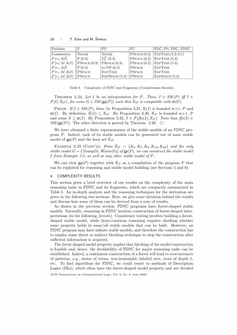
Problem F FD FC FDC, FN, FNC, FDNC
Consistency Trivial Trivial PSpace (6.2) ExpTime (5.2, 6.1)
P |=b A(~t) P (6.3) ΣP2 (6.3) PSpace (6.2) ExpTime (5.3)
P |=b ∃~x.A(~x) PSpace (6.3) PSpace (6.3) PSpace (6.2) ExpTime (5.3)
P |=c A(~t) P (6.3) co-NP (6.3) PSpace ExpTimeP |=c ∃~x.A(~x) PSpace ExpTime PSpace ExpTimeP |=c λ~x.A(~x) PSpace ExpSpace (5.4) PSpace ExpSpace (5.4)
Table I. Complexity of FDNC and Fragments (Completeness Results)
Theorem 3.34. Let I be an interpretation for P . Then, I ∈ SM (P ) iff I ∈F(G, KP ), for some G ∈ SM (gp(P )) such that KP is compatible with st(G).
Proof. If I ∈ SM (P ), then, by Proposition 3.21, K(I) is founded w.r.t. P andst(I). By definition, K(I) ⊆ KP . By Proposition 3.30, KP is founded w.r.t. Pand some S ⊇ st(I). By Proposition 3.32, I ∈ F(ffa(I), KP ). Note that ffa(I) ∈SM (gp(P )). The other direction is proved by Theorem 3.26.
We have obtained a finite representation of the stable models of an FDNC pro-gram P . Indeed, each of its stable models can be generated out of some stablemodel of gp(P ) and the knot set KP .
Example 3.35 (Cont’d). From KP = {K6,K7,K8,K12,K28} and the onlystable model G = {Young(b),Warm(b)} of gp(P ), we can construct the stable modelI from Example 3.2, as well as any other stable model of P .
We can view gp(P ) together with KP as a compilation of the program P thatcan be exploited for reasoning and stable model building (see Sections 5 and 6).
4. COMPLEXITY RESULTS
This section gives a brief overview of our results on the complexity of the mainreasoning tasks in FDNC and its fragments, which are compactly summarized inTable I. An in-depth analysis and the reasoning techniques for the derivation aregiven in the following two sections. Here, we give some intuition behind the resultsand discuss how some of them can be derived from a core of results.
As shown in the previous section, FDNC programs have forest-shaped stablemodels. Naturally, reasoning in FDNC involves construction of forest-shaped inter-pretations (in the following, forests). Consistency testing involves building a forest-shaped stable model, while brave/cautious reasoning requires checking whethersome property holds in some/all stable models that can be built. However, anFDNC program may have infinite stable models, and therefore the construction hasto employ some direct or indirect blocking technique to stop the construction aftersufficient information is acquired.
The forest-shaped model property implies that blocking of the model constructionis feasible and, hence, the decidability of FDNC for major reasoning tasks can beestablished. Indeed, a continuous construction of a forest will lead to reoccurrencesof patterns, e.g., states of terms, non-isomorphic labeled arcs, trees of depth 1,etc. To find algorithms for FDNC, we could resort to methods of DescriptionLogics (DLs), which often have the forest-shaped model property and are decided
ACM Transactions on Computational Logic, Vol. 9, No. 9, June 2099.

Decidable Nonmonotonic DLPs with Function Symbols · 19
by tableau methods with blocking. Unfortunately, such methods are not well-suitedin our case. First, they cannot easily handle minimality testing and are generally notworst-case optimal. Second, tableau methods are designed for consistency testing,while some important tasks from non-monotonic reasoning (e.g. brave reasoning)cannot always be polynomially reduced to consistency testing (see Table I).
Therefore, our algorithms for FDNC rely on the finite representation of stablemodels in terms of maximal founded sets of knots. In Section 5.1, we show how toderive the set KP of knots for a given FDNC program P in single exponential timein the size of P . This is possible as the number of distinct x-grounded knots isbounded by a single exponential. Given KP , several standard reasoning tasks canbe solved in time polynomial in the size of KP ; hence, overall they are in ExpTime.This includes consistency testing (Section 5.2), brave entailment of ground and exis-tential queries (Section 5.3), as well as cautious entailment of ground and existentialqueries (which is easily reduced to consistency testing). These upper bounds aretight for FDNC. It is easy to see that a decision procedure needs to explore forestswhose depths are bounded by a single exponential in the size of the input program.However, due to the disjunction or non-monotonic negation in an FDNC program,the number of such candidate forests may be too high for a procedure to traversethem in polynomial space. The ExpTime-hardness of consistency testing alreadyin FDC is proved in Section 5.2 by an encoding of an ExpTime-hard DescriptionLogic ALC, which is extended to FN in Section 6.1. The hardness of consistencytesting directly provides lower bounds for brave and cautious entailment of groundand existential queries. We note also that the ExpTime-completeness results forFDC and FN show that these fragments are equal in terms of problem solving ca-pacity: unlike in the propositional setting (cf. [Dantsin et al. 2001]), negation alonecan polynomially compensate disjunction and constraints, and vice versa.
For the fragment FC of FDNC, the picture is different. Its programs have theunique model property, i.e., if a stable model exists, it is unique. For the standardreasoning tasks, a procedure thus needs to navigate a unique forest searching for anode with a certain property, e.g., the one that causes an inconsistency, or satisfiesa query. Furthermore, the procedure needs to navigate only the depths bounded bya single exponential. Our algorithms navigate the forest by non-deterministicallyguessing the paths through function symbols and building necessary parts of astable model. They run in polynomial space and can, by Savitch’s Theorem [1970],turned into deterministic polynomial space algorithms. The PSpace-hardness ofconsistency testing is shown by a Turing machine encoding, which is extended toother standard reasoning tasks (see Section 6.2).
If we disallow non-monotonic negation and constraints, the complexity dropseven more. Consistency testing in both F and FD is trivial, while the complexityof ground entailment drops to lower levels of the polynomial hierarchy, and corre-sponds to the complexity of propositional logic programming. This is because con-sistency needs not be ensured, and the necessary conditions can be verified locallywithin polynomial distance from the graph part of the input program. Section 6.3discusses the results for F and FD.
The last row in Table I lists the complexity of open queries. Deciding cautiousentailment of open queries in FDNC is ExpSpace-complete and thus harder than
ACM Transactions on Computational Logic, Vol. 9, No. 9, June 2099.

20 · T. Eiter and M. Simkus
cautious entailment of existential queries. Intuitively, this is because to search fora term that satisfies a property in each stable model of a program, we must look atbranches beyond single exponential length. However, the length can be boundedby a double exponential, and we can thus manage to answer the query in singleexponential space; Section 5.4 provides the details. As noted in the preliminaries,in case of brave entailment, the semantics of open and existential queries coincide,and hence the complexity results on existential queries carry over to open queries.
The main entries in Table I are presented with references to the sections thatdiscuss the respective problems in detail. The other entries are justified as follows:
(1) Programs in F and FD are positive and without constraints, hence consistent.
(2) PSpace-hardness (resp. ExpTime-hardness) of P |=c ∃~x.A(~x) in F and FC
(resp. in FD and FDC) holds as consistency checking with constraints in FC (resp.FDC) is reducible to cautious inference. On the other hand, completeness also holdsas cautious inference is reducible to inconsistency testing in the standard way.
(3) Similarly, PSpace (resp. ExpTime) membership of P |=c A(~t), where P isa program in FC (resp. FDC, FN, FNC or FDNC), holds as the problem amountsto checking consistency of P ∪ {← A(~t)}. On the other hand, hardness holds as Pis inconsistent iff P |=c A′(t), where A′ is a fresh symbol and t is arbitrary.
(4) PSpace-completeness of P |=c λ~x.A(~x) in F and FC holds because thesefragments have the unique stable model property, and hence cautions entailment ofopen and existential queries coincide; the latter is PSpace-complete.
To ease presentation, we use a lemma that allows us to focus on unary queries.
Lemma 4.1. Let C be a complexity class in Table I, and let L be from the F
family. Then:
(i) If deciding program consistency for L is C-hard, then deciding brave entail-ment of queries (ground or existential, unary or binary) is also C-hard for L.
(ii) Brave entailment of unary existential (resp., ground) queries is C-completefor L iff brave entailment of binary existential (resp., ground) queries is C-complete for L.
(iii) Cautious entailment of unary open queries is C-complete for L iff cautiousentailment of binary open queries is C-complete for L.
For a proof of Lemma 4.1, we refer to the appendix. Intuitively, the first statementholds as brave reasoning involves a construction of a stable model containing acertain atom, which cannot be easier than constructing (or checking the existenceof) an arbitrary stable model. The second statement hinges on the fact that the classF allows rules A(y) ← R(x, y) and R(x, f(x)) ← A(x), by which brave entailmentof binary queries can be reformulated in terms of unary queries, and vice versa.Similarly, with rules in the syntax of F, one constructs reductions proving (iii).
5. COMPLEXITY OF FDNC
This section discusses the complexity of reasoning in FDNC and provides worst-case optimal algorithms together with the matching hardness results. The methodsfor consistency testing, deciding brave entailment of ground and existential queries
ACM Transactions on Computational Logic, Vol. 9, No. 9, June 2099.

Decidable Nonmonotonic DLPs with Function Symbols · 21
and cautious entailment of open queries rely on the finite representation of stablemodels in terms of the set KP of knots which, together with the set SM (gp(P )),captures all the stable models of an FDNC program P (see Theorem 3.34).
5.1 Deriving Maximal Founded Set of Knots
To derive KP , we proceed in two phases. In the first phase, we generate the set ofknots that surely contains KP . In the second phase, we remove some knots from itto ensure that it satisfies Definition 3.29.
To ease the presentation, for any knot set L, let st+1(L) = {st(K, s) | K ∈L,s∈ succ(K)}, i.e., st+1(L) is the set of all states of the successor terms of knots in L.
Definition 5.1 (All(P )). For an FDNC program P , let All(P ) be the smallestset of x-grounded knots satisfying the following conditions:
a) If U ∈ st(gp(P )) and K ∈ SM (P (U)), then K↓x ∈ All(P ).
b) If U ∈ st+1(All(P )) and K ∈ SM (P (U)), then K↓x ∈ All(P ).
Intuitively, All(P ) contains by construction each set of knots that is foundedw.r.t. P and some set of states S ⊆ st(P ). The first problem is that All(P ) mightcontain knots K that lack some successor knots, i.e., for some s ∈ succ(K) no K ′ isin All(P ) s.t. st(K, s) ≈ st(K ′,x) (condition (3.a) in Definition 3.19). On the otherhand, each knot in KP must be reachable from a state in st(P ) (condition (3.b)).These requirements are ensured by removing some knots from All(P ).
Definition 5.2 (bad(L)). For any set of x-grounded knots L, bad(L) is thesmallest subset of L such that K ∈ bad(L), if for some s∈ succ(K), either
a) no K ′ ∈L fulfills st(K, s)≈ st(K ′,x), or
b) for all K ′ ∈ L, st(K, s) ≈ st(K ′,x) implies K ′ ∈ bad(L).
Intuitively, obtaining the set All(P ) \ bad(All(P )) corresponds to iteratively re-moving from All(P ) the knots that have no successors (note that removing a knotfrom a set L might leave some other knots in L without a successor).
The following notion will help to ensure satisfaction of (3.b) of Definition 3.19.
Definition 5.3 (reachS(L)). For any set of x-grounded knots L and set of statesS, reachS(L) is the smallest set of knots such that:
a) if U ∈ S, K ∈ L and U ≈ st(K,x), then K ∈ reachS(L), and
b) if U ∈ st+1(reachS(L)), K ∈ L and U ≈ st(K,x), then K ∈ reachS(L).
Intuitively, reachS(L) are the knots in L reachable from the states in S. Indeed, ifreachS(L) = L, then L fulfills condition (3.b) of Definition 3.19 w.r.t. S.
Theorem 5.4. If P is an FDNC program, then KP = reachst(gp(P ))(LP ), whereLP = All(P ) \ bad(All(P )).
Proof. Let L = reachst(gp(P ))(All(P ) \ bad(All(P ))). We verify that L satisfiesthe conditions in Definition 3.29, i.e., L is the single ⊆-minimal set which containseach knot set L′ that is founded w.r.t. P and some S ⊆ st(gp(P )).
Indeed, every such L′ fulfills L′⊆All(P ); by construction of L, no K ∈L′ isremoved, thus L′ ⊆ L. To prove the result, it is thus sufficient to show that L itself
ACM Transactions on Computational Logic, Vol. 9, No. 9, June 2099.

22 · T. Eiter and M. Simkus
is founded w.r.t. P and some S⊆ st(gp(P )) (cf. Definition 3.19). The definition ofAll(P ) ensures that every K ∈L is stable w.r.t. P . Furthermore, the removal ofknots in bad(All(P )) and restriction to reachable knots ensures that every K ∈Lhas proper successors as in (3.a) of Definition 3.19, and has a proper predecessorsequence as in (3.b) that reaches a state in st(gp(P )) (we can set S suitably).
It is easy to see that we can compute KP in time at most single exponential inthe size of an FDNC program P . This is immediate from the following observations:
– The number of x-grounded knots over P is bounded by a single exponential inthe size of P . More precisely, the number is bounded by b(P ) = 2n+k·(n+m),when P has k function, n unary, and m binary predicate symbols.
– Computing All(P ) requires adding at most b(P ) x-grounded knots. Each suchknot has polynomial size and its stability is verifiable using a ΣP
2 = NPNP oracle.Thus, All(P ) is computable in time single exponential in the size of P .
– Computing bad(L) is polynomial in the size of L. Thus, All(P ) \ bad(All(P )) iscomputable in time single exponential in the size of P .
– The size of st(gp(P )) is bounded by a single exponential in the size of P .
– Computing reachS(L) is polynomial in the combined size of L and S.
5.2 Deciding Consistency
Once the set KP for an FDNC program P is derived, it can be readily used forconsistency testing. We will see that the resulting algorithm is worst-case optimal.
Theorem 5.5. For every FDNC program P , the following are equivalent:
(i) P is consistent.
(ii) For some G ∈ SM (gp(P )), the set KP is compatible with st(G).
Proof. If I ∈ SM (P ), then by Theorem 3.34 some G ∈ SM (gp(P )) exists suchthat KP is compatible with st(G). The converse is proved by Theorem 3.26.
By this theorem, to decide consistency of P we can search for a stable model Gof the program gp(P ) such that for each constant of P , KP can start the treeconstruction (i.e., KP is compatible with st(G)). We obtain the following result.
Theorem 5.6. Deciding whether an FDNC program is consistent is in ExpTime.
Proof. Deciding whether KP is compatible with st(G), for some G ∈ SM (gp(P )),is feasible in time polynomial in n + m, where m is the size of KP and n is the sizeof SM (gp(P )). Overall, this can be done in time single exponential in the size ofP , since both m and n are single exponential in the size of P . Since SM (gp(P )) iscomputable in single exponential time, the result follows from Theorem 5.5.
As we have pointed earlier already, we can see KP together with gp(P ) as acompilation of the FDNC program P . Out of this compilation, we can graduallybuild a stable model of P by continuing the tree construction for some stable modelG of gp(P ) using knots from KP (and every stable model of P results by properchoices). Here the hard part is computing such a G, which depending on thecomplexity of function-free programs is ΣP
2 -hard already for FD, NP-hard alreadyfor FN, and polynomial for F and FC. Checking the compatibility of KP with
ACM Transactions on Computational Logic, Vol. 9, No. 9, June 2099.

Decidable Nonmonotonic DLPs with Function Symbols · 23
Mapping knowledge base K
Θ(K) =S
α∈K{Π(α)}
Mapping axioms and assertions
Π(C(a)) = pC(a) Π(R(a, b)) = pR(a, b)
Π(C ⊑D) = (∀x)(π(C, x)→ π(D, x))
Mapping concepts
π(⊤, X) = ⊤ π(C ⊔D, X) = π(C, X) ∨ π(D, X)
π(A, X) = pA(X) π(C ⊓D, X) = π(C, X) ∧ π(D, X)
π(⊥, X) = ⊥ π(∀R.C, X) = (∀y)(pR(X, y)→ π(C, y))
π(¬C, X) = ¬π(C, X) π(∃R.C, X) = (∃y)(pR(X, y) ∧ π(C, y))
Note: X is a meta-variable that is replaced by an actual variable.
Fig. 4. Semantics of the DL ALC by mapping to first-order logic
st(G) is polynomial, and each tree expansion step using a knot from KP is feasiblewith low (clearly polynomial) cost. Note that this model-building technique iscomplementary to computing a stable model of an ordinary (function-free) logicprogram, and may be realized on top of stable model engines like DLV or Smodels.
In the following, we show that the algorithm emerging from Theorem 5.5 is worst-case optimal. The proof is by a polynomial-time translation of consistency testingin the Description Logic ALC, which is ExpTime-hard, to consistency testing inFDC. The translation is interesting in its own right, as it provides a translation ofthe core of expressive Description Logics into logic programming.
Definition 5.7 (ALC Syntax). Let C ⊇ {⊤,⊥}, R and I denote the sets ofconcept, role, and individual names, respectively. Inductively, each C ∈ C is aconcept, and if C,D are concepts and R is a role, then C ⊓D, C ⊔D, ¬C, ∀R.C,and ∃R.C are concepts. If C ∈ C, then C and ¬C are literal concepts.
A general concept inclusion axiom (GCI) is of form C ⊑ D where C, D areconcepts. An assertion is of form C(a) or R(a, b), where a, b ∈ I, R ∈ R, andC ∈ C. An ALC knowledge base is a finite set of GCIs and assertions.
Each ALC knowledge base K has a model-theoretic semantics, which is given viaa mapping of K into a set of sentences in first-order logic, shown in Figure 4 (seee.g. [Hustadt et al. 2004] for details). The major reasoning task in ALC is decidingthe consistency of a given K, i.e., that of the first-order theory Θ(K).
We now provide a polynomial time translation of normalized ALC knowledgebases K into FDC programs PK such that K is consistent iff PK is consistent. Nor-malized knowledge bases obey certain structural constraints which makes presentingthe translation easier.
Definition 5.8 (ALC Normal Form). An ALC knowledge base K is in nor-mal form, if its GCI axioms are of one of the following forms:
(T1) A0 ⊓ . . . ⊓An⊑B0 ⊔ . . . ⊔Bm, (T4) A0⊑∃R.B0,(T2) A0 ⊓ . . . ⊓An⊑⊥, (T5) A0⊑∀R.B0,(T3) ⊤⊑B0 ⊔ . . . ⊔Bm,
ACM Transactions on Computational Logic, Vol. 9, No. 9, June 2099.

24 · T. Eiter and M. Simkus
Axioms of K Rules of PK
(T1) A0 ⊓ . . . ⊓An ⊑B0 ⊔ . . . ⊔Bm B0(x) ∨ . . . ∨Bm(x)← A0(x), . . . , An(x)
(T2) A0 ⊓ . . . ⊓An ⊑⊥ ← A0(x), . . . , An(x)
(T4) A⊑ ∃R.C R′(x, f(x))← A(x)
R(x, y)← R′(x, y)
C(y)← R′(x, y)
(T5) A⊑ ∀R.C C(y)← A(x), R(x, y)
A(a) A(a)←;
R(a, b) R(a, b)←;
where n ≥ 0, f is fresh function symbol, R′ is a fresh binary predicate symbol.
Table II. Translating ALC into FDNC
where n,m ≥ 0, and each Ai and Bj is from C, but is neither ⊤ nor ⊥.3 Moreover,if K is in normal form and does not contain axioms of type (T3), then K is safe.4
Importantly, we can normalize any ALC knowledge base K efficiently.
Proposition 5.9. Given any ALC knowledge base K, we can obtain in lineartime a safe knowledge base K′ in normal form that is consistent iff K is consistent.
The proof, which is based on well-known definitional form transformations, isgiven in the appendix. We are now ready to define the translation. For any safeknowledge base K in normal form, let PK denote the FDNC program that resultsafter applying the translation rules in Table II.
Proposition 5.10. Let K be a safe knowledge base in normal form. Then K isconsistent iff PK is consistent.
Proof. It is easy to verify that PK is a rule-representation of the first-order the-ory that is obtained from Θ(K) by applying Skolemization and a satisfiability pre-serving transformation for the axioms of type (T4). By Herbrand’s Theorem [1971],PK is consistent iff Θ(K) consistent.
Note that PK is in fact positive and constructible in linear time from K. Hence,Propositions 5.9–5.10 and the well-known ExpTime-hardness of ALC [Schild 1991]imply that deciding consistency of FDC and FDNC programs is ExpTime-hard.Combined with Theorem 5.6, we establish the completeness result.
Theorem 5.11. Checking consistency of FDC and FDNC programs is ExpTime-complete.
5.3 Brave Entailment of Queries
As we did for consistency checking, we exploit the set KP for a program P toprovide algorithms for brave reasoning. We first discuss entailment of existentialunary atomic queries, and then of ground queries. The idea behind the method isto perform some “back-propagation” of unary predicate symbols in the set of knots.
3For a similar normal form for the weaker Description Logic EL++, see [Baader et al. 2005].4We require safety because applying the transformation Π to an axiom ⊤⊑ B0 ⊔ . . . ⊔ Bm leadsto the formula ∀x.B0(x) ∨ . . . ∨ Bm(x) which, in turn, cannot be stated as a safe rule in FDNC
syntax.
ACM Transactions on Computational Logic, Vol. 9, No. 9, June 2099.
Decidable Nonmonotonic DLPs with Function Symbols · 25
Definition 5.12 (reachA(L)). For every set L of x-grounded knots and unarypredicate symbol A, let reachA(L) be the smallest subset of L such that:
(a) if K ∈ L and A(x) ∈ K, then K ∈ reachA(L), and
(b) if K ′ ∈ reachA(L) is a possible successor of K ∈ L, i.e., for some s∈ succ(K)we have st(K, s)≈ st(K ′,x), then K ∈ reachA(L).
Intuitively, K ∈ reachA(L) means that, starting from K, a sequence of possiblesuccessor knots will eventually reach a knot containing A(x). Since KP togetherwith SM (gp(P )) captures the stable models of P , we have the following:
Theorem 5.13. For every program P , the following statements are equivalent:
(A) P |=b ∃x.A(x).
(B) Some G ∈ SM (gp(P )) exists such that (i) KP is compatible with st(G), and (ii)for some constant c and K ∈ KP , st(G, c) ≈ st(K,x) and K ∈ reachA(KP ).
Theorem 5.13 provides us with an algorithm, since brave entailment of existentialqueries can be decided by verifying the condition (B) of the theorem. As easily seen,the condition is verifiable in time single exponential in the size of the program P .Indeed, computing reachA(KP ) requires time quadratic in the size of KP , or singleexponential in the size of P . Once KP , reachA(KP ), and SM (gp(P )) are computed,the conditions in (B) are verifiable in time polynomial in the combined size of KP ,reachA(KP ), and SM (gp(P )). Hence, (B) can be verified in time single exponentialin the size of P , that is, for a given FDNC program, the problem of deciding whetherit bravely entails a unary existential query is in ExpTime. On the other hand, dueto Theorem 5.11 and Lemma 4.1, we know that brave entailment of unary existentialqueries is ExpTime-hard already for FDC. Therefore, we conclude the following.
Theorem 5.14. For FDC and FDNC programs, brave entailment of an exis-tential unary query is ExpTime-complete. The same holds for binary existentialqueries (see Lemma 4.1).
The method for deciding brave entailment of ground queries is based on an adap-tation of the algorithm for existential queries.
Definition 5.15 (goalq(L)). Let q = A(t) be a ground atom and L be a set ofx-grounded knots. Let T be the set of subterms of the term t. Then goalq(L) is thesmallest relation over L×T such that:
(a) if K ∈ L and A(x) ∈ K, then 〈K, t〉 ∈ goalq(L), and
(b) if there exist (i) K ∈ L with f(x) ∈ succ(K) and (ii) K ′ ∈ L s.t. st(K, f(x)) ≈st(K ′,x) and 〈K ′, f(v)〉 ∈ goalq(L), then 〈K, v〉 ∈ goalq(L).
Intuitively, goalq(L) tries to construct proofs of q by backward chaining in L; aproof succeeds, if some pair 〈K, c〉 is obtained where c is constant symbol. Due tothe properties of KP , we obtain:
Theorem 5.16. Let P be an FDNC program and q a ground unary query. Sup-pose c is the single constant occurring in q. The following two are equivalent:
(A) P |=b q.
ACM Transactions on Computational Logic, Vol. 9, No. 9, June 2099.

26 · T. Eiter and M. Simkus
(B) Some G ∈ SM (gp(P )) exists such that (i) KP is compatible with st(G), and(ii) some K ∈ KP exists such that st(G, c) ≈ st(K,x) and 〈K, c〉 ∈ goalq(KP ).
By similar arguments as for existential queries, we can see that checking condition(B) is feasible in time single exponential in the size of P and q. Note that computinggoalq(KP ) is feasible in time polynomial in the size of KP and q, or single exponentialin the size of P and q. Once KP , goalq(KP ), and SM (gp(P )) are computed, theconditions in (B) can be verified in time polynomial in the combined size of KP ,goalq(KP ), and SM (gp(P )), each of which is single exponential in the size of Pand q. Thus brave entailment of unary ground queries by FDNC programs isin ExpTime. To establish completeness, recall Theorem 5.11 and item (ii) inLemma 4.1.
Theorem 5.17. For FDC and FDNC programs, brave entailment of unary groundqueries (resp., binary ground queries) is ExpTime-complete.
5.4 Cautious Entailment of Open Queries
In the previous sections, we presented methods for brave entailment of existentiallyquantified or ground queries. As shown in Section 4, cautious reasoning can beeasily reduced to consistency testing. All these tasks are ExpTime-complete forFDNC. This section deals with cautious entailment of open queries, which turnsout to be harder (under widely adopted beliefs in complexity theory).
Like for other reasoning methods discussed, we base our method on the set KP ofan FDNC program P . As we have seen, each stable model of P can be constructedby taking a compatible graph and building a tree for each constant. Indeed, ifP |=c A(t) holds, each tree construction starting at the constant of t from knots inKP must eventually reach t satisfying A. We introduce the following notion.
Definition 5.18 (Converging Sequence). Let A be a unary predicate sym-bol of P . A nonempty sequence [L0
c, L1
f1, . . . , Ln
fn], were each Li ⊆ KP is nonempty,
c is a constant, and f1, . . . , fn are function symbols, is called a converging sequencefor A (w.r.t. KP ) if the following hold:
(1) for each K ∈ Lj−1, where 1 ≤ j ≤ n, fj(x) ∈ succ(K);
(2) for each K ∈ Lj−1, where 1 ≤ j ≤ n, and each K ′ ∈ KP , st(K, fj(x)) ≈st(K ′,x) implies K ′ ∈ Lj;
(3) if K ∈ Ln, then A(x) ∈ K.
Furthermore, we use the following notion for knots that can start models. Fora constant c, let seeds(c, P ) be the set of all knots K ∈ KP such that for someG ∈ SM (gp(P )) we have st(K,x) ≈ st(G, c) and KP is compatible with st(G).
Proposition 5.19. Let P be a consistent FDNC program and let λx.A(x) be anopen query. Then P |=c λx.A(x) iff some converging sequence s = [L0
c, L1
f1, . . . , Ln
fn]
for A exists, where L0 = seeds(c, P ).
The proposition above characterizes cautious entailment of open queries in termsof existence of converging sequences. To provide an algorithm, we next show thatthe length of converging sequences is double exponentially bounded in the size ofthe initial program.
ACM Transactions on Computational Logic, Vol. 9, No. 9, June 2099.

Decidable Nonmonotonic DLPs with Function Symbols · 27
Algorithm openQueries (FDNC program P , open query λx.A(x))Output: true iff there exists t s.t. P |=c A(t)
if P is inconsistent then
return trueend if
Guess some constant c of P ;
L := seeds(c, P );repeat
if A(x) ∈ K for each K ∈ L then
return trueend if
Guess some f ∈ F ;if there exists K ∈ L such that f(x) /∈ succ(K) then
return falseelse
Laux := {K′ ∈ KP | st(K′,x) ≈ st(K, f(x)) ∧K ∈ L};
L := Laux;
i := i + 1end if
until i = |F | × 2|KP | + 1
return false
Fig. 5. Non-deterministic procedure for cautious entailment of open queries; KP is assumed to beprecomputed, F is the set of function symbols of P .
Proposition 5.20. For every converging sequence [L0
c, L1
f1, . . . , Ln
fn] for A, there
exists a converging sequence [L0
c,
L′
1
f ′
1
, . . . ,L′
m
f ′
m] for A such that m ≤ |F | × 2|KP | + 1,
where F is the set of function symbols occurring in P .
Proof. There are only |F | × 2|KP | distinct pairs Lf
of a function symbol f and
a set of knots L ⊆ KP . Suppose s = [L0
c, L1
f1, . . . , Ln
fn] is a converging sequence for
A and Lf
is an element of s that occurs more than once, first at position 0 < k and
last at position k < l. It is easy to verify that [L0
c, L1
f1, . . . , Lk
fk, Ll+1
fl+1, . . . , Ln
fn] is a
converging sequence for A where Lf
occurs only once. Note that the first element of
the sequence is preserved. It follows that a converging sequence s′ for A exists thatdoes not contain duplicates of its elements, while its first element is L0
c. Indeed, s′
cannot be longer than |F | × 2|KP | + 1, and thus the claim holds.
The next theorem follows directly from Proposition 5.19 and Proposition 5.20.
Theorem 5.21. Let P be an FDNC program and let λx.A(x) be an open query.Then P |=c λx.A(x) iff P is inconsistent or some converging sequence [L0
c, L1
f1, . . . ,
Ln
fn] for A exists, where L0 = seeds(c, P ) and n ≤ |F | × 2|KP | + 1.
Based on this theorem, we present in Figure 5.4 an algorithm that decides cau-tious entailment of open queries by checking the existence of a converging sequenceof at most double exponential length. We assume that the set KP for the in-put program P is precomputed. The procedure guesses a sequence of functionssymbols and verifies the conditions in Definition 5.18. It can be implemented torun in non-deterministic exponential space; indeed, storing the set KP and thedouble exponential counter requires at most exponential space, while the rest of
ACM Transactions on Computational Logic, Vol. 9, No. 9, June 2099.
28 · T. Eiter and M. Simkus
the constructs require at most linear space. By Savitch’s Theorem [1970], we canturn the algorithm into an algorithm using exponential space, which establishes theExpSpace-membership. By a generic Turing machine encoding, we show that theproblem is ExpSpace-hard, even for FD and FN programs (see Appendix).
Theorem 5.22. Cautious entailment of open queries in FD, FN, FNC, FDC
and FDNC programs is ExpSpace-complete.
6. COMPLEXITY OF FRAGMENTS
In this section, we consider the complexity of reasoning in the fragments of FDNC.Some reasoning tasks are already covered by the results of Section 5 and the dis-cussion in Section 4, including cautious entailment of existential queries in FD (cf.Theorem 5.11 and Lemma 4.1) and of open queries in general (cf. Theorem 5.22).
We first show that in FN, all reasoning tasks remain as hard as in full FDNC. Allother reasoning tasks that remain to be considered are at most PSpace-complete,and in some cases at low levels of the polynomial hierarchy.
6.1 Reasoning in FN and FNC
We show that the consistency problem for FDC reduces in polynomial time tothe consistency problem for FN. Since the reasoning tasks that we considered(consistency and brave entailment) are ExpTime-complete for FDC and FDNC,the reduction implies that they are all ExpTime-complete for FN and FNC.
The plan is as follows. We first construct, given an arbitrary FDC program P ,an FN program fr(P ) (the frame program) whose stable models intuitively coincidewith the minimal (forest-shaped) Herbrand interpretations for P . We then struc-turally transform P into an FN program P ′ such that P is consistent iff the FN
program P ′ ∪ fr(P ) is consistent.
Definition 6.1 (Frame Program fr(P )). For each predicate Q of P , let Qbe a fresh predicate symbol of the same arity, Let Dom and S be fresh unary andbinary predicate symbols, respectively. Then fr(P ) is the FN program with the rules
(F1) Dom(c) ← , (F5) A(x) ← Dom(x), not A(x)
(F2) S(c, d) ← , (F6) A(x) ← Dom(x), not A(x)
(F3) S(x, f(x)) ← Dom(x), (F7) R(x, y) ← S(x, y), not R(x, y),
(F4) Dom(y) ← S(x, y), (F8) R(x, y) ← S(x, y), not R(x, y),
for each pair c, d of constants of P , each function symbol f of P , and each unaryand binary predicate symbol A and R of P , respectively.
Proposition 6.2. Given an interpretation I ⊆ HBfr(P ), I ∈ SM (fr(P )) iff I isforest-shaped, and
(1) S(c, d) ∈ I, for each pair c, d of constants of P ,
(2) Dom(t) ∈ I, for each term t ∈ I,
(3) S(t, f(t)) ∈ I, for each t ∈ I and each function symbol f of P ,
(4) |{A(t), A(t)} ∩ I| = 1, for each t ∈ I and each unary predicate A of P , and
(5) S(s, t) ∈ I implies |{R(s, t), R(s, t)} ∩ I| = 1, for each pair s, t ∈ I and eachbinary predicate R of P .
ACM Transactions on Computational Logic, Vol. 9, No. 9, June 2099.
Decidable Nonmonotonic DLPs with Function Symbols · 29
Intuitively, fr(P ) generates a set of forest-shaped interpretations for P . Nextwe show how to filter out the interpretations that do not satisfy the rules in P .If some interpretation I remains, then P is consistent. Note that such I wouldnot necessarily correspond to a minimal model of P . For technical reasons, weassume that the rules of type (R6) occurring in P are non-disjunctive. It is easyto see that such rules can be eliminated from P in linear time while preservingconsistency: replace each rule R1(x, f1(x))∨ . . .∨Rn(x, fk(x))← B0(x), . . . , Bl(x)by rules A1(x)∨ . . .∨An(x)← B0(x), . . . , Bl(x) and Ri(x, fi(x))← Ai(x) for eachi∈{1, . . . , n}, where each Ai is a fresh predicate symbol.
Definition 6.3 (Transformation). For an FDC program P as described, wedenote by tf(P ) the FN program fr(P ) ∪ P ′, where P ′ is the FN program obtainedfrom P by replacing each rule
W1(~t1) ∨ . . . ∨Wn(~tn)← Q1(~v1), . . . , Qm(~vm) ∈ Pwith a rule
C(~t1)← Q1(~v1), . . . , Qm(vm), W1(~t1), . . . , Wn(~tn), not C(~t1),
where C is a fresh predicate symbol with the arity of ~t1, and n,m ≥ 0.
We note that for simplicity, all rules are rewritten, including non-disjunctive ruleand constraints. Indeed, tf(P ) is an FN program; literals Wi(~ti) in the head ofan initial rule can be shifted to their “complements” Wi(~ti) in the body withoutviolating the syntax of FN programs. This would not be the case if disjunctive headswere allowed for rules (R6). The following holds (for a proof, see the appendix).
Proposition 6.4. The program P is consistent iff tf(P ) is consistent.
We showed how to transform an FDC program into an FN program while pre-serving consistency. As easily verified, the translation is polynomial in the size ofthe initial program P (more precisely, quadratic in the size of P due to the facts(F2) of fr(P ); the rest is linear). Therefore, recalling ExpTime-completeness ofconsistency testing in FDNC (Theorem 5.11), we conclude.
Corollary 6.5. Checking consistency of FN and FNC programs is ExpTime-complete.
The ExpTime-completeness of consistency checking for FN allows us to obtainsimilar results for brave query entailment. Since consistency testing is reducible tobrave entailment (see Lemma 4.1), and since brave entailment of existential andground queries is ExpTime-complete (see Theorems 5.14 and 5.17), we obtain:
Corollary 6.6. For FN and FNC programs, brave entailment of unary (resp.,binary, by Lemma 4.1) ground or existential queries is ExpTime-complete.
6.2 Reasoning in FC
We show that reasoning in FC is easier than in FDNC: consistency and brave rea-soning reduce to PSpace-completeness. To obtain these results, we cannot exploitthe maximal founded set of knots of a program as its size can be exponentiallylarge. Nevertheless, the semantic characterization centering around Theorem 3.13enables reasoning from FC programs by iterative construction of knots. The fol-lowing result, which holds for full FDNC, provides a basis for reasoning in FC.
ACM Transactions on Computational Logic, Vol. 9, No. 9, June 2099.

30 · T. Eiter and M. Simkus
Theorem 6.7. Let P be an FDNC program. The following two are equivalent:
(i) SM (P ) 6= ∅.
(ii) There exists some G ∈ SM (gp(P )) such that, for each constant c of P , a setof knots exists that is founded w.r.t. P and {st(G, c)}.
Proof. For the “(i) to (ii)” direction, assume that I is a stable model of P .By Theorem 3.13, ffa(I) is a stable model of gp(P ). So let G = ffa(I). ByProposition 3.21, we know that the set of knots K(I) is founded w.r.t. P andst(G). Simply take some ⊆-minimal set L of knots closed under the following rules:
a) L contains some K ∈ K(I) such that st(G, c) ≈ st(K,x), and
b) if K ∈L and s∈ succ(K), then some K ′ ∈L exists such that st(K, s)≈ st(K ′,x).
Indeed, due to foundedness of K(I), the set L can be constructed and is foundedw.r.t. P and {st(G, c)}. For the other direction, assume (ii) holds. Let Lc denote aset of knots that is founded w.r.t. P and {st(G, c)}. Let C be the set of constants ofP . Due to Proposition 3.28, the set L =
⋃c∈C Lc is a set of knots that is founded
w.r.t. P and st(G). Then Theorem 3.26 proves the claim.
The key feature of FC is the unique model property, i.e., if an FC program hasa minimal model, then it is unique. From Theorem 6.7, we know that to decidewhether a FC program is consistent we can proceed in two steps:
(1) Check the existence of the single minimal model G of gp(P ). If it exists, thenproceed to the next step. Otherwise, P is not consistent.
(2) Check whether for each constant c of P , a set of knots exists that is foundedw.r.t. P and {st(G, c)}. If so then P is consistent, otherwise not.
Indeed, G is computable in time polynomial in the size of P . For the second step,notice that the local programs for P also have the unique-model property. Thisimplies a unique set L that is founded w.r.t. P and {U}, where U is a state.
To decide the second step, in Figure 6 we present a generic non-deterministicprocedure checkCondition. The procedure takes as input an FDNC program P ,a state U , and a Boolean function that maps states to Boolean values. In theprocedure, the value b(P ) is the number of distinct x-grounded knots over thesignature of P . As it was already argued, b(P ) = 2n+k·(n+m), where n and m arethe numbers of unary and binary predicate symbols of P , respectively, and k is thenumber of function symbols in P .
Let cond1 be a Boolean function that maps each state U to true if the programP (U) is inconsistent, and to false otherwise.
Proposition 6.8. Let P be an FC program, and let U be a state. There ex-ists a set of knots that is founded w.r.t. P and {U} iff no run of the procedurecheckCondition(P,U, cond1) returns true.
Proof. The “only if” direction is trivial, while for the other direction, we cansimply collect all the knots that appeared at any run of the algorithm. It is easyto verify that such a collection is a set that is founded w.r.t. P and {U}.
The algorithm checkCondition(P,U, cond1) runs in polynomial space. The pro-cedure keeps only a counter that counts up to a single exponential; this requires
ACM Transactions on Computational Logic, Vol. 9, No. 9, June 2099.

Decidable Nonmonotonic DLPs with Function Symbols · 31
func checkCondition (program P , state U , function cond)repeat
if cond(U) = true then
return trueend if ;Choose K ∈ MM (P (U)) and s ∈ succ(K);
Let U be a state obtained from st(K, s) by substituting s with x;i := i + 1
until i = b(P );
return false
Fig. 6. Non-deterministic procedure for PSpace algorithms
only polynomial space. Note that the procedure at each iteration works only on asingle local program that is of polynomial size. This local program has a uniquemodel property and, hence, representing its models requires polynomial space also.
Indeed, to decide the second step, we need to make only a linear number ofcalls to checkCondition. Summing up, both steps to decide consistency of P arefeasible in co-NPSpace w.r.t. to the size of P . By Savitch’s Theorem [1970], weknow co-NPSpace = PSpace.
Theorem 6.9. Deciding whether a given FC program is consistent is in PSpace.
On the other hand, PSpace-hardness of the problem is shown by a Turing ma-chine simulation (see Lemma A.4 in the appendix). Thus we obtain the following.
Theorem 6.10. For FC programs, checking consistency is PSpace-complete.
Since FC programs have the single-stable model property, brave entailment ofexistential queries can be easily expressed by constraints that are allowed in FC.
Proposition 6.11. Let P be an FC program. Then P |=b ∃x.A(x) iff P isconsistent and P ∪ {← A(x)} is not consistent.
The proposition implies that brave entailment of an existential unary query in FC
can be polynomially reduced to consistency checking in FC. Recalling that the taskis PSpace-hard (Lemma 4.1), we conclude the following.
Corollary 6.12. For FC programs, brave entailment of unary existential queriesis PSpace-complete. The same holds for binary existential queries (see Lemma 4.1).
In a similar fashion, we prove PSpace-completeness for ground queries. Thefollowing proposition is helpful.
Proposition 6.13. Let P be an FC program and let A(t) be a ground atom suchthat t = fn(. . . f1(c0) . . .). Let P ′ result from P by adding the following rules: (a)C0(c0)← , (b) R(x, fi+1(x))← Ci(x), for 0 ≤ i < n, (c) Ci+1(y)← Ci(x), R(x, y),for 0 ≤ i < n, (d) D(x)← Cn(x), A(x), and (e) ← D(x), where C0, . . . , Cn, R andD are fresh predicates. Then P |=b A(t) iff P is consistent and P ′ is not consistent.
The proposition implies that brave entailment of a ground unary query in FC
program P can be decided by adding polynomially many rules to P and making twoconsistency checks, and hence is polynomially reducible to consistency checking inFC. Since the latter is PSpace-hard by Lemma 4.1, we have the following result.
ACM Transactions on Computational Logic, Vol. 9, No. 9, June 2099.

32 · T. Eiter and M. Simkus
Theorem 6.14. For FC programs, brave entailment of unary ground queries isPSpace-complete. The same holds for binary queries (see Proposition 4.1).
6.3 Reasoning in F and FD
As F and FD programs are positive and constraint-free, they are always consistent.We discuss here brave entailment of existential queries together with brave andcautious entailment of ground queries; PSpace- and ExpTime-completeness ofcautious entailment of existential queries in F and FD, respectively, follows fromthe results for consistency testing in FC and FDC (see observation (2) in Section 4).
For a given F program P , deciding P |=b ∃x.A(x) is feasible in polynomial space(see Corollary 6.12). On the other hand, the problem is easily seen to be PSpace-hard; this can be shown by a simple adaptation of the Turing machine simulationfor Theorem 6.10 (see Lemma A.5).
Theorem 6.15. For F programs, brave entailment of unary existential queries isPSpace-complete. The same holds for binary existential queries (see Lemma 4.1).
For FD programs, PSpace-completeness of brave existential queries is not straight-forward, since they may have several minimal models and hence the task can notbe simply reduced to consistency testing as for F. The use of constraints leads toFDC, where consistency testing is already ExpTime-complete.
The strategy is to use the non-deterministic procedure checkCondition fromSection 6.2 for consistency testing in FC. To this end, we observe that the semanticcharacterization of stable models of FDNC allows us conclude the following.
Theorem 6.16. Let P be a FD program. The following two are equivalent:
(i) P |=b ∃x.A(x).
(ii) There exists G ∈ MM (gp(P )), a constant c of P , and a set of knots L foundedw.r.t. P and {st(G, c)} such that L contains some knot K with A(x)∈K.
Let q = ∃x.A(x) be a query and P be an FD program. The theorem above suggestsa method to decide whether P |=b q holds. The crucial point is to have a procedurefor deciding whether for a given state U over P , there exists a set of knots L thatis founded w.r.t. P and {U} and contains some knot K such that A(x) ∈ K.
Let cond2 be a Boolean function that maps each world state U to true if A(x) ∈U , and to false otherwise.
Proposition 6.17. Let U be a state, and P be an FD program. The followingtwo are equivalent.
(i) Some knot set L founded w.r.t. P and {U} and K ∈L exist such that A(x)∈K.
(ii) Some execution of checkCondition(P,U, cond2) returns true.
Proof. (i) ⇒ (ii): this holds since the size of L is bounded by b(P ).(ii) ⇒ (i): consider the sequence of knots that was constructed during the run of
the procedure that returned true. Since P has no constraints, this sequence can bealways augmented to a founded set by computing the missing successors knots.
By similar arguments as for consistency checking in FC, checkCondition runsin polynomial space in the input size. Note that traversing the states of constants
ACM Transactions on Computational Logic, Vol. 9, No. 9, June 2099.

Decidable Nonmonotonic DLPs with Function Symbols · 33
that occur in the minimal models of gp(P ) is feasible in polynomial space. Hence,condition (ii) in Theorem 6.16 is testable in polynomial space using a PSpaceoracle; overall, this amounts to polynomial space. As brave entailment of existentialqueries for FD programs is PSpace-hard (see Lemma 4.1), we conclude:
Theorem 6.18. For FD programs, brave entailment of unary existential queriesis PSpace-complete. The same holds for binary existential queries (see Lemma 4.1).
In contrast to existential queries, brave and cautious reasoning with groundqueries is easier in F and FD than in FC and FN. The methods are based onconstructing only relevant parts of stable models to answer a given query. SinceF and FD do not allow for constraints, we do not need to care about the globalconsistency of interpretations. By the relevant part of a model, we essentially meana sequence of knots that is constructed following the path encoded in the term t ofa ground query A(t). The following proposition elaborates on that.
Proposition 6.19. Suppose P be is an FD program and A(t) a ground atom inwhich as single constant c occurs. Let l = 〈s1, . . . , sn〉 be the list of subterms of tordered by increasing term depth, i.e., s1 = c and sn = t. Then the following hold:
1. P |=b A(t) if and only if (⋆) there exists some stable model G of gp(P ) and asequence 〈K1, . . . ,Kn〉 of stable knots with roots s1, . . . , sn, resp., such that:
(a) st(G, s1) = st(K1, s1),
(b) si+1 ∈ succ(Ki) and st(Ki, si+1) = st(Ki+1, si+1), where 1 ≤ i < n, and
(c) A(sn) ∈ Kn.
2. P 6|=c A(t) if and only if (⋆⋆) there exists some model G of gp(P ) and a sequence〈K1, . . . ,Kn〉 of knots with roots s1, . . . , sn, respectively, such that:
(a) st(G, s1) = st(K1, s1),
(b) si+1 ∈ succ(Ki) and st(Ki, si+1) = st(Ki+1, si+1), where 1 ≤ i < n,
(c) Ki is a model of P (st(Ki, si)), where 1 ≤ i ≤ n, and
(d) A(sn) 6∈ Kn.
Proposition 6.19 (whose proof is in the appendix) allows us to derive complexityresults for ground queries. To ease presentation, the characterization above is viawitnessing knot sequences: for brave entailment via a witness for entailment and forcautious entailment via a witness of a counter-model. Note that in (2.c), the knotsare not necessarily stable. Stability is not needed, and in fact would hinder findingcounter-models in nondeterministic polynomial time (due to stability testing).
Suppose P is an F program and A(t) a ground query. Since P is a Horn pro-gram, the local programs for P have least models computable in polynomial time.Moreover, the least model of gp(P ) is also computable in polynomial time. Hence,P |=b A(t) can be decided according to Proposition 6.19 by constructing in poly-nomial time the least model of gp(P ) and the unique sequence of knots. Hence,P |=b A(t) is in P. On the other hand, since P has the least model, P |=b A(t) iffP |=c A(t). Hence, P |=c A(t) is also in P.
Next suppose that P is an FD program and A(t) a ground query. As easilyseen, testing condition (⋆) for P is in ΣP
2 : indeed, guess an interpretation I forgp(P ) and a suitable knot sequence 〈K1, . . . ,Kn〉 over P ’s signature; this results in
ACM Transactions on Computational Logic, Vol. 9, No. 9, June 2099.

34 · T. Eiter and M. Simkus
a polynomial-size structure. One can then check in polynomial time with an NPoracle whether I is minimal and each knot Ki satisfies the conditions in (⋆).
To decide P 6|=c A(t), it suffices to verify the condition (⋆⋆) in Proposition 6.19.Since (⋆⋆) does not involve minimality of models, it is decidable in NP. Indeed,we may guess an interpretation for gp(P ) and a candidate sequence of knots overthe signature of P . Deciding then whether the structure satisfies (⋆⋆) is feasible inpolynomial time. Hence, P 6|=c A(t) is in NP, while P |=c A(t) is in co-NP.
It is not difficult to see that the given upper bounds are tight, since they cor-respond to complexity of brave and cautious reasoning in the propositional case.Simply consider fragments Fp of F and FDp of FD that allow only for rules of type(R1), unary facts, and only one constant. Indeed, any propositional Horn (resp.propositional positive disjunctive program) can be rewritten in LogSpace into anFp (resp. FDp) program while preserving the set of minimal models (up to renam-ing of atoms). This implies that brave/cautious reasoning in propositional Hornand positive disjunctive logic programs are LogSpace-reducible to brave/cautiousentailment of ground unary queries in F and FD programs respectively. Since braveentailment over positive propositional disjunctive programs is ΣP
2 -complete andcautious entailment is co-NP-complete, while both tasks are P-complete for Hornprograms (see e.g. [Dantsin et al. 2001]), we obtain completeness results for ourformalisms.
Theorem 6.20. For FD programs, brave (resp., cautious) entailment of unaryground queries is ΣP
2 -complete (resp. co-NP-complete). For F programs, both prob-lems are P-complete. All results extend to binary queries (see Lemma 4.1).
7. HIGHER-ARITY FDNC
We present here a decidable extension of FDNC that supports predicate and func-tion symbols of higher arities, and allows for more succinct and convenient knowl-edge representation in practice. This will be illustrated by a plain planning scenario(for a more detailed discussion, we refer the interested reader to Appendix B).
As already illustrated by the previous examples, FDNC supports naturally mod-eling of possibly infinite evolutions of a set of propositions. Indeed, for a term t,the unary predicates (i.e., the propositions) that hold for it can be used via rules ofFDNC to define the unary predicates that hold for the term f(t), where f(t) can beviewed as a follow-up time point. However, a propositional setting is inconvenientfor many action domains, and the use for parameters for more compact representa-tion is needed. They allow to represent actions that, for instance, move an objectx from a location l1 to the location l2. Hence, special predicate names for eachpossible combination of x, l1, and l2 as in a propositional setting can be avoided.(This is, e.g., widely used in [Baral 2002].)
In what follows, we assume that N1 and N2 are disjoint sets of predicate namesof arities at least 1 and 2, respectively.
Definition 7.1 (Global/Local Positions). Given an atom A(t1, . . . , tn) withA ∈ N1 or a term f(t1, . . . , tn), its local positions are 1, . . . , n − 1 and its globalposition is n. Similarly, given an atom A(t1, . . . , tn) with A ∈ N2, its local posi-tions are 1, . . . , n− 2 and its global positions are n− 1 and n. An atom A(~t) withA ∈ N1 (resp., A ∈ N2) is g-unary (resp., g-binary).
ACM Transactions on Computational Logic, Vol. 9, No. 9, June 2099.

Decidable Nonmonotonic DLPs with Function Symbols · 35
Definition 7.2 (Higher-Arity FDNC program). A higher-arity FDNC pro-gram is a finite disjunctive logic program whose rules are of the following forms:
(R1)∨k
i=1 Ai(~vi, x) ← B0( ~u0, x),∧l
j=1 B±j ( ~uj , x)
(R2)∨k
i=1 Ri(~vi, x, y) ← P0( ~u0, x, y),∧l
j=1 P±j ( ~uj , x, y)
(R3)∨k
i=1 Ri(~vi, x, fi(~ti, x)) ← P0( ~u0, x, g0( ~w0, x)),∧l
j=1 P±j ( ~uj , x, gj( ~wj , x))
(R4)∨k
i=1 Ai(~vi, y) ← P0( ~u0, x, y),∧l
j=1 P±j ( ~uj , x, y),
∧m
j=1 B±j ( ~wj , x),
∧n
j=1 C±j (~tj , y)
(R5)∨k
i=1 Ai(~vi, f(~v, x)) ← P0( ~u0, x, f(~v, x)),∧l
j=1 P±j ( ~uj , x, f(~v, x)),
∧m
j=1 B±j ( ~wj , x),
∧n
j=1 C±j (~tj , f(~v, x))
(R6)∨k
i=1 Ri(~vi, x, fi(~ti, x)) ← B0( ~u0, x),∧l
j=1 B±j ( ~uj , x)
(R7)∨k
i=1 Ai(~ti, b) ∨∨l
i=1 Ri(~vi, c, d) ←∧m
j=1 B±j ( ~uj , b
′),∧n
j=1 P±j ( ~wj , c
′, d′),
where k, l,m, n ≥ 0, and
– all Ai and Bj are from N1, and all Ri and Pj are from N2,
– the tuples ~v, ~w, and all ~vi, ~ti, ~uj, ~wj are tuples of variables or constants.
– b, c, d, b′, c′, d′ are constants,
– x and y do not occur in local positions of atoms and function symbols, and
– each rule r is safe, i.e., each of its variables occurs in body+(r).
The restrictions on the variable interaction allow us to transform higher-arityFDNC programs naturally into ordinary FDNC programs, which enables the usageof reasoning methods from the previous sections. In the following, we present thetransformation and a use case of a higher-arity FDNC program.
Definition 7.3 (FDNC Reduction). Let P be a higher-arity FDNC program.Let ld(P ) be the set of constants occurring in the local positions of atoms in P .Given a set of constants C, every rule r′ that results from r by substituting eachvariable occurring in a local position of some atom of r with some c ∈ C is aparameter-ground instance of r w.r.t. C; the set of all such r′ is denoted by gr(r, C).The parameter-grounding of P is the program pgr(P ) = {r′ ∈ gr(r, ld(P )) | r ∈ P}.
The FDNC-reduction of P , red(P ), results from P by replacing each g-unaryatom A(t1, . . . , tn) (resp., g-binary atom R(t1, . . . , tn)) occurring in pgr(P ) with anatom At1,...,tn−1
(tn) (resp., Rt1,...,tn−2(tn−1, tn)). Similarly, the FDNC-reduction of
an interpretation I for P is defined as red(I) = {At1,...,tn−1(tn) | A(t1, . . . , tn) ∈
I, A ∈ N1} ∪ {Rt1,...,tn−2(tn−1, tn) | R(t1, . . . , tn) ∈ I, R ∈ N2}.
The following result is then not difficult to establish.
ACM Transactions on Computational Logic, Vol. 9, No. 9, June 2099.

36 · T. Eiter and M. Simkus
Theorem 7.4. Let P be a higher-arity FDNC program. Then an interpretationI is a stable model of P iff red(I) is a stable model of red(P ).
Proof. We analyze the impact of restricted variable interaction in higher-arityFDNC. As easily verified, the atoms that can be justified (by program rules) in thestable models are of the particular form. Let P be a higher-arity FDNC program,and let pterms(P ) be the set of proper terms defined as the smallest set such that
a) if c ∈ HUP is a constant, then c ∈ pterms(P );
b) if t ∈ HUP is a complex term such that (1) in its local positions there areonly constants from ld(P ), and (2) in its global positions are the terms frompterms(P ), then t ∈ pterms(P ).
Note that pterms(P ) is closed under subterms. Let patoms(P ) be the set of allproper atoms for P , which are the atoms in HBP that have constants from ld(P )in the local positions and terms from pterms(P ) in the global positions.
Due to the syntax of higher-arity FDNC, given any (Herbrand) interpretationI of P , a rule r ∈ P I contains a non-proper atom iff it contains a non-properatom in the body. Hence, every J ∈ MM (P I) such that J ⊆ I must satisfyJ ⊆ patoms(P ). Let P ′ result from Ground(P ) by deleting each rule that contains
some atom A /∈ patoms(P ). Then MM (P I) = MM (P ′I) holds. This implies thatSM (P ) = SM (P ′). Moreover, only proper atoms can be justified in stable mod-els of P , i.e., I ⊆ patoms(P ) holds for each I ∈ SM (P ). Trivially, SM (P ′) ={I | red(I) ∈ SM (red(P ′))}. On the other hand, it is easily seen that red(P ′) =Ground(red(pgr(P ))). Since SM (Ground(red(pgr(P ))) = SM (red(pgr(P )))), it fol-lows that I ∈ SM (P ) iff red(I) ∈ SM (red(pgr(P ))), as claimed.
Since red(P ) is finite, higher-arity FDNC programs inherit decidability from or-dinary FDNC programs. However, their complexity is higher (by one exponential)in the general case. This is not surprising, since the parameter-grounding of P isexponential in the size of P .5
An exponential blow-up only occurs when arbitrarily many parameters are al-lowed in rules, i.e., if the number of variables that can occur in local position isunbounded. If the maximal number of variables in local positions is fixed, then theparameter-grounding is polynomial in the size of a higher-arity program, and ourcomplexity results carry over for higher-arity FDNC.
Below is an example of an application of higher-arity FDNC programs to com-pactly represent the blocks world problem. For this purpose, we enhance FDNC
programs with “strong” negation ¬P (~x) [Gelfond and Lifschitz 1991], which is ex-pressed in the core language as usual: view ¬P as a fresh predicate symbol andadd constraints ← P (~x),¬P (~x).
5The hardness results for ExpTime, co-NExpTime, and co-NExpTimeNP corresponding to P,co-NP, and ΣP
2 , respectively, follow from the complexity of ordinary function-free logic programs[Dantsin et al. 2001]; ExpSpace and 2-ExpSpace corresponding to PSpace and ExpSpace can beobtained by generalizing the given Turing machine encodings. As for 2-ExpTime correspondingto ExpTime, one can show ExpTime-hardness of reasoning in ordinary FDC and FN by adapting
the given encoding of PSpace Turing machines into FC to alternating PSpace-Turing machines(which capture ExpTime). With parameters, this can be further lifted to alternating ExpSpace= 2-ExpTime.
ACM Transactions on Computational Logic, Vol. 9, No. 9, June 2099.
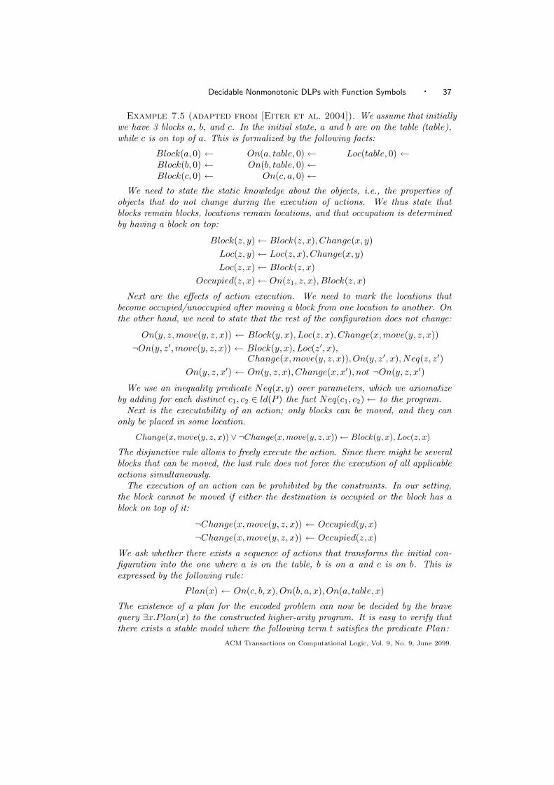
Decidable Nonmonotonic DLPs with Function Symbols · 37
Example 7.5 (adapted from [Eiter et al. 2004]). We assume that initiallywe have 3 blocks a, b, and c. In the initial state, a and b are on the table (table),while c is on top of a. This is formalized by the following facts:
Block(a, 0) ← On(a, table, 0)← Loc(table, 0) ←Block(b, 0) ← On(b, table, 0)←Block(c, 0) ← On(c, a, 0)←
We need to state the static knowledge about the objects, i.e., the properties ofobjects that do not change during the execution of actions. We thus state thatblocks remain blocks, locations remain locations, and that occupation is determinedby having a block on top:
Block(z, y)← Block(z, x), Change(x, y)
Loc(z, y)← Loc(z, x), Change(x, y)
Loc(z, x)← Block(z, x)
Occupied(z, x)← On(z1, z, x), Block(z, x)
Next are the effects of action execution. We need to mark the locations thatbecome occupied/unoccupied after moving a block from one location to another. Onthe other hand, we need to state that the rest of the configuration does not change:
On(y, z,move(y, z, x)) ← Block(y, x), Loc(z, x), Change(x,move(y, z, x))
¬On(y, z′,move(y, z, x)) ← Block(y, x), Loc(z′, x),Change(x,move(y, z, x)), On(y, z′, x), Neq(z, z′)
On(y, z, x′) ← On(y, z, x), Change(x, x′), not ¬On(y, z, x′)
We use an inequality predicate Neq(x, y) over parameters, which we axiomatizeby adding for each distinct c1, c2 ∈ ld(P ) the fact Neq(c1, c2)← to the program.
Next is the executability of an action; only blocks can be moved, and they canonly be placed in some location.
Change(x, move(y, z, x)) ∨ ¬Change(x, move(y, z, x))← Block(y, x), Loc(z, x)
The disjunctive rule allows to freely execute the action. Since there might be severalblocks that can be moved, the last rule does not force the execution of all applicableactions simultaneously.
The execution of an action can be prohibited by the constraints. In our setting,the block cannot be moved if either the destination is occupied or the block has ablock on top of it:
¬Change(x,move(y, z, x)) ← Occupied(y, x)
¬Change(x,move(y, z, x)) ← Occupied(z, x)
We ask whether there exists a sequence of actions that transforms the initial con-figuration into the one where a is on the table, b is on a and c is on b. This isexpressed by the following rule:
Plan(x) ← On(c, b, x), On(b, a, x), On(a, table, x)
The existence of a plan for the encoded problem can now be decided by the bravequery ∃x.P lan(x) to the constructed higher-arity program. It is easy to verify thatthere exists a stable model where the following term t satisfies the predicate Plan:
ACM Transactions on Computational Logic, Vol. 9, No. 9, June 2099.

38 · T. Eiter and M. Simkus
t = move(c, b,move(b, a,move(c, table, 0)))
The term t encodes the plan of moving c to the table, b on top of a, and finally con top of b. The same t is also an answer for the cautious open query λx.P lan(x)to the program, and encodes a secure plan for the goal.
However, if the initial location of b were not known, i.e., On(b, table, 0) ← isreplaced by On(b, table, 0) ∨On(b, c, 0)←, then the above plan is no longer secure,as the first step is not executable in the case where b is on top of c. Here, the answer
t = move(c, b,move(b, a,move(c, table,move(b, table, 0))))
to the cautious open query λx.P lan(x) encodes a secure plan.
We finally remark that higher-arity FDNC programs allow to encode (fragmentsof) the predicate version of the action language K, but omit further discussion here.
8. RELATED WORK
DatalognS. A close relative of FDNC is DatalognS [Chomicki and Imielinski 1993;Chomicki 1995], which provides an extension of the Datalog language in deductivedatabases with function symbols more liberal in spirit than in FDNC programs. Thesyntax of DatalognS allows for rules in which atoms with complex terms affect atomswith less complex terms, which is not allowed in FDNC programs. On the otherhand, DatalognS features neither of disjunction, negation, and constraints, and thushas to be compared with F; modulo minor differences, ordinary and higher-arity F
programs are DatalognS programs.Chomicki and Imielinski [1993] presented an algebraic approach to compile the
least Herbrand models of DatalognS programs (i.e., their single stable models) viahomomorphisms into finite structures, on which query answering can be performed.Different representations of these structures, viz. a graph specification and an equa-tional specification that uses a congruence relation, have been described and ana-lyzed; other representation methods for restricted classes of programs in the liter-ature were also discussed. The compilation technique in [Chomicki and Imielinski1993] does not extend to FDNC programs, which can have multiple (even infinitelymany) stable models. The techniques of knots, which constitute building blocksof stable models, handles multiplicity of models by knot sharing, such that everystable model can be readily assembled from knots.
Notably, ordinary and higher-arity F have lower complexity than DatalognS , atleast regarding data complexity (which was considered in [Chomicki and Imielinski1993]). As reported there, cautious entailment of ground queries in DatalognS isExpTime-complete with respect to data complexity, i.e., w.r.t. the size of the set offacts in the program. On the other hand, cautious entailment of ground queries fromF programs (which coincides with brave entailment) is feasible in polynomial time;the same holds for higher-arity F programs when the number of parameters in eachrule is bounded by a constant, since then the parameter grounding pgr(P ) and theFDNC-reduct of P have polynomial size; thus, the ground query can be answered inpolynomial time when the rules are fixed. This continues to hold when facts addedto P may also involve function symbols (in global positions only): complex termsin facts can be compiled away in polynomial time (e.g., by partial instantiation andintroducing fresh predicate and constant symbols for ground terms). Hence, w.r.t.
ACM Transactions on Computational Logic, Vol. 9, No. 9, June 2099.

Decidable Nonmonotonic DLPs with Function Symbols · 39
data complexity, our F programs constitute a meaningful, tractable fragment ofDatalognS . In [Chomicki 1995], different evaluation strategies for query answeringfrom DatalognS programs have been considered; by their relationship to F programs,they can applied to the latter as well.
Finitely recursive and finitary programs. Our class FN, which results from FDNC
by disallowing constraints and disjunction, is in essence (modulo elimination of rules(R2) and (R4)) a decidable subclass of the Finitely Recursive Programs (FRPs)[Bonatti 2004; Baselice et al. 2007]. FRPs are normal logic programs P with func-tion symbols such that in Ground(P ) each atom depends only on finitely manyatoms. In this formalism, inconsistency checking is r.e.-complete and brave groundentailment is co-r.e.-complete in general [Baselice et al. 2007]. For FN and ourfull class FDNC, which implicitly obeys the condition of FRPs, these problems areExpTime-complete. On the other hand, FN is not a subclass of the Finitary Pro-grams (FPs) [Bonatti 2004], which are those RFPs in whose grounding only finitelymany atoms occur in odd cycles. For FPs, consistency checking is decidable, andbrave and cautious entailment are decidable for ground queries but r.e.-completefor existential atomic queries. Note that for FN, all these problems are decidablein exponential time. Finally, the explicit syntax of FN and all other fragmentsof FDNC allows effective recognition of their programs. Recognition of FRPs andFPs, instead, suffer from undecidability.
Omega-restricted logic programs. For logic programs with negation under sta-ble model semantics, ω-restricted logic programs have been presented in [Syrjanen2001]. These are normal logic programs with function symbols of arbitrary aritiesand an unbounded number of variables, but have restricted syntax to ensure thefinite-model property, i.e., that finite answer sets always exist. The restriction is ageneralization of classical stratification based on the existence of an acyclic orderingof the atom dependencies, which adds a special ω-stratum that holds all unstrat-ifiable predicates of the logic program. In contrast, our FDNC programs do notexclude cyclic dependencies, and they lack the finite model property. Furthermore,FDNC programs have lower computational complexity. While consistency testingin general ω-restricted programs is 2-NExpTime-complete, the test can be done inExpTime for ordinary and in 2-ExpTime for higher-arity FDNC programs.
Local extended conceptual logic programs. Another formalism related to FDNC-programs are Local Extended Conceptual Logic Programs (LECLPs) [Heymans et al.2005] which evolved from [Heymans 2006]. Such programs are function-free buthave answer sets over open domains, i.e., of the grounding of P with an arbitrarysuperset of the constants in P . LECLPs are syntactically restricted to ensure theforest-shape model property of answer sets. Deciding consistency of an LECLP Pis feasible in 3-NExpTime, as one can ground P with double exponentially manyconstants in the size of P , and then use a standard ASP solver. For FDNC, decidingthe consistency is ExpTime-complete and thus less complex.
Comparing the expressiveness of LECLPs and FDNC is intricate due the differentsettings. At least, both formalisms can encode certain description logics (e.g.,ALC).LECLPs may be more expressive than FDNC programs, since the expressive DLALCHOQ is reducible to satisfiability in LECLPs. On the other hand, LECLPs
ACM Transactions on Computational Logic, Vol. 9, No. 9, June 2099.

40 · T. Eiter and M. Simkus
deviate from the general intuition behind the minimal model semantics of logicprograms. So-called free rules of the form p(x)∨not p(x)←; allow to unfoundedlyadd atoms for p in an answer set. FDNC, instead, has no free rules, and each atomin a stable model of P must be justified from the facts of P .
Reductions of Description Logics to ASP. Reductions of Description Logics toASP have been considered e.g. in [Alsac and Baral 2001; Baral 2002; Swift 2004;Hustadt et al. 2004; Heymans and Vermeir 2003; Heymans et al. 2005]. Alsac andBaral [2001; 2002] gave a reduction of ALCQI to normal function-free logic pro-grams (i.e., Datalog with stable negation), which was geared towards the Herbranddomain of a knowledge base; by adding rules to generate inductively terms witha function symbol, they extended it to infinite domains. Their reduction is, in asense, less constructive than the one given here and others, where function symbolsare used to handle existential quantifiers by Skolemization. Swift [2004] reporteda reduction of deciding satisfiability of ALCQI concepts to Datalog with stablenegation, which exploits the finite model property of this problem. Heymans et al.[2003; 2005] reduced SHIQ (which subsumes ALCQI) to their Conceptual LogicPrograms and extensions; however, they used answer sets over open domains.
Most relevant for the present paper is Hustadt et al.’s [2004]. They reducedreasoning in SHIQ to the evaluation of a positive disjunctive Datalog program.The program is generated in three steps. First, the knowledge base is translatedinto first-order logic in a standard way. After that, resolution and superpositiontechniques are applied to saturate a clausal form of the transformation. Finally,function symbols are removed using new constant symbols.
The reduction of ALC to FDC in Section 5.2 is, in essence, similar to others anda close relative of the one of Hustadt et al. described above. The main differencesto the latter are with respect to their second step, where our method uses knots forcompilation, and that our method aims at model building while the one in [Hustadtet al. 2004] is geared towards query answering. Notably, the disjunctive Datalogprogram constructed in [Hustadt et al. 2004] is generally exponential in the size ofthe initial DL knowledge base (but is evaluable in co-NP), while the FDC programis polynomial (but may need exponential time for evaluation).
Furthermore, the reduction contributes in two respects. First, the knowledge baseis rewritten (very efficiently) on the DL syntax side into a normal form, rather thanon the first-order logic side after the mapping. Second, a transformation into FDC
opens the possibility to use any dedicated evaluation algorithm for such programs,beyond a specific method (like the one in this paper).
Reasoning about Actions and Planning. As already discussed in the previoussections, the use of non-monotonic logic programs under answer set semantics as atool for solving problems in reasoning about actions has been considered in manypapers, including [Dimopoulos et al. 1997; Lifschitz 1999; Baral 2002; Eiter et al.2004; Tu et al. 2007; Son et al. 2006; Son et al. 2005; Morales et al. 2007]. Thework presented here adds to these other works by providing an underpinning of thecomputational properties of non-monotonic logic programs with functions symbolsthat naturally emerge in this context, and, importantly, capture indefinitely longaction sequences. They help in assessing the complexity of particular problems and
ACM Transactions on Computational Logic, Vol. 9, No. 9, June 2099.

Decidable Nonmonotonic DLPs with Function Symbols · 41
may be useful to show that tractability can be achieved in some cases. Furthermore,our results provide algorithms to solve problems expressed in the language.
9. CONCLUSION
In line with efforts to pave the way for effective Answer Set Programming engineswith function symbols [Bonatti 2004; Baselice et al. 2007], we presented FDNC
programs as a decidable class of disjunctive logic programs with function symbolsunder stable model semantics.
FDNC and its subclasses are a powerful tool for knowledge representation andreasoning for some applications involving infinite processes and objects, like evolv-ing action domains. They are, by their intrinsic complexity, the proper fragment oflogic programs to capture secure (alias conformant) planning in declarative actionlanguages with a transition-based semantics like K, C, and similar languages, whichis an ExpSpace-complete problem.
Notably, FDNC programs can have infinitely many and infinitely large stablemodels. To finitely represent those models, we introduced a technique that allowsto reconstruct stable models as forests from so called knots from maximal foundedset of knots. The finite representation technique allowed us to define an elegantdecision procedure for brave reasoning in FDNC, and may also be exploited foroffline knowledge compilation to speed up online reasoning and model building, byprecomputing and storing the knots of a program.
Furthermore, we have characterized the complexity of reasoning in FDNC pro-grams, which is lower than in the most popular of the recent approaches to enhanceAnswer Set Programming with functions symbols. FDNC and its subclasses pro-vide effective syntax for expressing problems in PSpace, ExpTime, and ExpSpaceusing logic programs with function symbols.
The are several avenues for future research. One is to generalize the syntax ofFDNC, while keeping decidability and benign semantic properties. An interestingsuch extension is to allow rules of the form R(y, x) ← R(x, y). The ability todefine inverse relations, which are common in expressive DLs and related modallogics, would allow for the bi-directional flow of information between elements inthe domain; the resulting programs are, as seem by a reduction to monadic second-order logic over trees SkS, still decidable. While the forest-shaped model propertywould remain, such relations are problematic due to the stable model semantics. Inpresence of inverse relations, testing the minimality of interpretation for a programbecomes more involved. Intuitively, the justification of atoms in an interpretationcan no longer be verified by only considering the structurally less complex atoms.To deal with these issues, we plan to generalize the knot-based technique for thefinite representation of stable models.
FDNC and, in particular, the finite representation of stable models is a promis-ing basis of developing algorithms for answering more complex queries than thoseconsidered in this paper. Since FDNC easily captures some basic DLs, the algo-rithms developed for FDNC may be applicable also in other domains. In general,query answering algorithms need to construct a set of models in order to answer thequery. The algorithms using the maximal founded set of knots as an input, wouldbe relieved from computationally expensive model building since the relevant part
ACM Transactions on Computational Logic, Vol. 9, No. 9, June 2099.

42 · T. Eiter and M. Simkus
of the model can be built using knots without the need to ensure the consistency.Finally, implementation of FDNC programs is a subject of future work. Since
stable knots are defined as stable models of local programs (which are finite propo-sitional disjunctive logic programs), the implementation will certainly export partsof reasoning to one of the highly optimized answer set solvers currently available. Inparticular, recent extensions of the DLV system like DLVHEX, which implementshex programs [Eiter et al. 2005] that feature external function calls (by which lim-ited Skolemization could be simulated), may be attractive for this.
ELECTRONIC APPENDIX
The electronic appendix for this article can be accessed in the ACM Digital Li-brary by visiting the following URL: http://www.acm.org/pubs/citations/
journals/tocl/2099-9-9/p99-URL.
Acknowledgments
We are grateful to the reviewers of this and the preliminary LPAR 2007 paperfor their useful comments and suggestions for improvements, as well as to PieroBonatti, Nicola Leone, Stijn Heymans and many further colleagues.
REFERENCES
Alsac, G. and Baral, C. 2001. Reasoning in description logics using declarative logic program-
ming. Tech. rep., Dep. Computer Science and Engineering, Arizona State University.
Andreka, H. and Nemeti, I. 1978. The generalised completeness of Horn predicate logics asprogramming language. Acta Cybernetica 4, 1, 3–10.
Asparagus. Homepage (since 2005). http://asparagus.cs.uni-potsdam.de/.
Baader, F., Brandt, S., and Lutz, C. 2005. Pushing the EL envelope. See Kaelbling and
Saffiotti [2005], 364–369.
Baader, F., Calvanese, D., McGuinness, D., Nardi, D., and Patel-Schneider, P. F., Eds.2003. The Description Logic Handbook: Theory, Implementation and Applications. CambridgeUniversity Press.
Baral, C. 2002. Knowledge Representation, Reasoning and Declarative Problem Solving. Cam-
bridge University Press.
Baselice, S., Bonatti, P. A., and Criscuolo, G. 2007. On finitely recursive programs. In Proc.23rd Int’l Conference on Logic Programming (ICLP 2007). LNCS 4670. Springer, 89–103.
Bonatti, P. A. 2004. Reasoning with infinite stable models. Artificial Intelligence 156, 1, 75–111.
Cadoli, M. and Donini, F. 1997. A survey on knowledge compilation. AI Comm. 10, 3-4,
137–150.
Chomicki, J. 1995. Depth-bounded bottom-up evaluation of logic programs. Journal of LogicProgramming 25, 1, 1–31.
Chomicki, J. and Imielinski, T. 1993. Finite representation of infinite query answers. ACMTransactions on Database Systems 18, 2, 181–223.
Dantsin, E., Eiter, T., Gottlob, G., and Voronkov, A. 2001. Complexity and expressive
power of logic programming. ACM Computing Surveys 33, 3, 374–425.
Darwiche, A. and Marquis, P. 2002. A knowledge compilation map. Journal of ArtificialIntelligence Research 17, 229–264.
Dimopoulos, Y., Nebel, B., and Koehler, J. 1997. Encoding planning problems in nonmono-
tonic logic programs. In Proc. European Conference on Planning 1997 (ECP-97). LNCS 1348.Springer, 169–181.
Dix, J., Furbach, U., and Nerode, A., Eds. 1997. Proc. 4th International Conference on LogicProgramming and Nonmonotonic Reasoning (LPNMR’97). LNCS 1265. Springer.
ACM Transactions on Computational Logic, Vol. 9, No. 9, June 2099.

Decidable Nonmonotonic DLPs with Function Symbols · 43
Eiter, T., Faber, W., Leone, N., Pfeifer, G., and Polleres, A. 2003. A logic programmingapproach to knowledge-state planning, II: The dlv
K system. Artif. Intell. 144, 1-2, 157–211.
Eiter, T., Faber, W., Leone, N., Pfeifer, G., and Polleres, A. 2004. A logic program-ming approach to knowledge-state planning: Semantics and complexity. ACM Transactions on
Computational Logic 5, 2, 206–263.
Eiter, T. and Gottlob, G. 1997. Expressiveness of stable model semantics for disjunctive logicprograms with functions. Journal of Logic Programming 33, 2, 167–178.
Eiter, T., Gottlob, G., and Mannila, H. 1997. Disjunctive datalog. ACM Transactions onDatabase Systems 22, 3, 364–418.
Eiter, T., Ianni, G., Schindlauer, R., and Tompits, H. 2005. A uniform integration of higher-
order reasoning and external evaluations in answer set programming. See Kaelbling and Saffiotti[2005], 90–96.
Eiter, T., Leone, N., Mateis, C., Pfeifer, G., and Scarcello, F. 1997. A deductive systemfor non-monotonic reasoning. See Dix et al. [1997], 364–375.
Gebser, M., Kaufmann, B., Neumann, A., and Schaub, T. 2007. Clasp : A conflict-driven
answer set solver. In Proc. LPNMR-07, C. Baral, G. Brewka, and J. S. Schlipf, Eds. LectureNotes in Computer Science, vol. 4483. Springer, 260–265.
Gelfond, M. and Lifschitz, V. 1991. Classical negation in logic programs and disjunctivedatabases. New Generation Computing 9, 3/4, 365–386.
Gelfond, M. and Lifschitz, V. 1992. Representing actions in extended logic programming. In
Proc. Joint Int’l Conf. and Symp. on Logic Programming (JICSLP-92). MIT Press, 559–573.
Giunchiglia, E. and Lifschitz, V. 1998. An action language based on causal explanation:Preliminary report. In Proc. 15th National Conf. Artificial Intelligence (AAAI-98). 623–630.
Hanks, S. and McDermott, D. V. 1987. Nonmonotonic logic and temporal projection. ArtificialIntelligence 33, 3, 379–412.
Haslum, P. and Jonsson, P. 1999. Some results on the complexity of planning with incomplete
information. In Proc. 5th European Conf. Planning (ECP-99). LNCS 1809, 308–318.
Herbrand, J. 1971. Logical Writings. Harvard University Press. Edited by Warren D. Goldfarb.
Heymans, S. 2006. Decidable open answer set programming. Ph.D. thesis, Theoretical ComputerScience Lab, Department of Computer Science, Vrije Universiteit Brussel.
Heymans, S., Nieuwenborgh, D. V., and Vermeir, D. 2005. Nonmonotonic ontological andrule-based reasoning with extended conceptual logic programs. In Proc. 2nd European Semantic
Web Conference (ESWC-05), LNCS 3532. Springer, 392–407.
Heymans, S. and Vermeir, D. 2003. Integrating semantic web reasoning and answer set program-ming. In Proc. Workshop on Answer Set Programming (ASP-2003), M. de Vos and A. Provetti,Eds. CEUR Workshop Proc., vol. 78. CEUR-WS.org, 194–208.
Hustadt, U., Motik, B., and Sattler, U. 2004. Reducing SHIQ-description logic to disjunctive
datalog programs. In Proceedings KR-2004. AAAI Press, 152–162.
Hustadt, U., Schmidt, R. A., and Georgieva, L. 2004. A survey of decidable first-orderfragments and description logics. J. Relational Methods in Computer Science 1, 251–276.
Itai, A. and Makowsky, J. A. 1987. Unification as a complexity measure for logic programming.Journal of Logic Programming 4, 105–117.
Kaelbling, L. P. and Saffiotti, A., Eds. 2005. IJCAI-05, Proc. 19th International Joint
Conference on Artificial Intelligence. Professional Book Center.
Levesque, H. J., Pirri, F., and Reiter, R. 1998. Foundations for the situation calculus. Elec-tronic Transactions on Artificial Intelligence 2, 159–178.
Lifschitz, V. 1999. Answer set planning. In Proc. 16th International Conference on LogicProgramming (ICLP-99), D. D. Schreye, Ed. The MIT Press, 23–37.
Lifschitz, V. 2002. Answer set programming and plan generation. Artif. Intell. 138, 39–54.
Lifschitz, V. and Turner, H. 1994. Splitting a logic program. In Proc. 11th InternationalConference on Logic Programming (ICLP-94), P. V. Hentenryck, Ed. The MIT Press, 23–37.
Marek, V. W. and Remmel, J. B. 2003. On the expressibility of stable logic programming.Theory and Practice of Logic Programming 3, 4-5, 551–567.
ACM Transactions on Computational Logic, Vol. 9, No. 9, June 2099.

44 · T. Eiter and M. Simkus
Marek, V. W. and Truszczynski, M. 1999. Stable models and an alternative logic programmingparadigm. In The Logic Programming Paradigm – A 25-Year Perspective, Springer, 375–398.
Marek, W., Nerode, A., and Remmel, J. 1992. How complicated is the set of stable models ofa recursive logic program? Annals of Pure and Applied Logic 56, 119–135.
Marek, W., Nerode, A., and Remmel, J. 1994. The stable models of a predicate logic program.Journal of Logic Programming 21, 3, 129–153.
Morales, A. R., Tu, P. H., and Son, T. C. 2007. An extension to conformant planning usinglogic programming. In Proc. 20th Int’l Joint Conference on Artificial Intelligence (IJCAI-07).AAAI Press/IJCAI, 1991–1996.
Motik, B., Horrocks, I., and Sattler, U. 2007. Bridging the gap between OWL and relationaldatabases. In Proc. 16th Int’l Conf. World Wide Web (WWW-07). ACM, 807–816.
Niemela, I. 1999. Logic programming with stable model semantics as constraint programmingparadigm. Annals of Mathematics and Artificial Intelligence 25, 3–4, 241–273.
Niemela, I. and Simons, P. 1997. Smodels - an implementation of the stable model and well-founded semantics for normal lp. See Dix et al. [1997], 421–430.
Savitch, W. J. 1970. Relationships between nondeterministic and deterministic tape complexi-ties. Journal of Computer and System Sciences 4, 2, 177–192. ISSN 1439-2275.
Schild, K. 1991. A correspondence theory for terminological logics: Preliminary report. In Proc.12th Int’l Joint Conf. on Artificial Intelligence (IJCAI-91). Morgan Kaufmann, 466–471.
Son, T. C., Baral, C., Tran, N., and McIlraith, S. A. 2006. Domain-dependent knowledgein answer set planning. ACM Transactions on Computational Logic 7, 4, 613–657.
Son, T. C., Tu, P. H., Gelfond, M., and Morales, A. R. 2005. Conformant planning fordomains with constraints-a new approach. In Proc. 20th National Conf. Artificial Intelligence(AAAI-05). AAAI Press/MIT Press, 1211–1216.
Swift, T. 2004. Deduction in ontologies via ASP. In Proc. 7th Int’l Conf. on Logic Programmingand Nonmonotonic Reasoning (LPNMR-04). LNCS/LNAI 2923, Springer, 275–288.
Syrjanen, T. 2001. Omega-restricted logic programs. In Proc. 6th Int’l Conf. on Logic Program-ming and Nonmonotonic Reasoning (LPNMR-01). LNCS 2173, Springer, 267–279.
Tu, P. H., Son, T. C., and Baral, C. 2007. Reasoning and planning with sensing actions,incomplete information, and static causal laws using answer set programming. Theory and
Practice of Logic Programming 7, 4, 377–450.
Woltran, S. 2005. Answer set programming: Model applications and proofs-of-concept. Tech.
Rep. WP5, Working Group on Answer Set Programming (WASP, IST-FET-2001-37004). July.Available at http://www.kr.tuwien.ac.at/projects/WASP/report.html.
Received January 2008; revised December 2008; accepted February 2009
ACM Transactions on Computational Logic, Vol. 9, No. 9, June 2099.

Decidable Nonmonotonic DLPs with Function Symbols · App–1
This document is the online-only appendix to:
FDNC: Decidable Nonmonotonic Disjunctive Logic Programs
with Function Symbols
THOMAS EITER and MANTAS SIMKUS
Technische Universitat Wien
ACM Transactions on Computational Logic, Vol. 9, No. 9, June 2099, Pages 99–44.
A. PROOFS AND CONSTRUCTIONS
A.1 Auxiliary Lemma
Proof of Lemma 4.1. The statement (i) follows directly from the fact that inthe basic fragment F we can state unary and binary facts. Indeed, P is consistentiff P ∪ {Q(c) ←} |=b ∃x.Q(x), where Q and c are fresh symbols not occurring inP . Hence, whenever a fragment allows for unary facts, the consistency problem inthat fragment can be reduced in logarithmic space to brave entailment of existentialunary queries in the same fragment. The same can be shown for binary existentialqueries, and also for ground queries.
It is easy to see that the statement (ii) holds for existential queries. Indeed, foran arbitrary logic program P , the following hold:
1) P |=b ∃x, y.R(x, y) iff P ∪ {Q(x)← R(x, y)} |=b ∃x.Q(x), and
2) P |=b ∃x.A(x) iff P ∪ {W (x, f(x))← A(x)} |=b ∃x, y.W (x, y),
where Q, W , and f are fresh symbols not occurring in P . This defines a logarithmicspace reduction from brave entailment of binary existential queries to unary ones,and vice versa. Since even in the basic F fragment the syntax allows to add thenecessary rule, the claim follows.
As in the case above, by utilizing additional rules, brave entailment of binaryground queries can be reduced in logarithmic space to brave entailment of unaryground queries, and vice versa. Hence, the statement (ii) also holds for groundqueries. We state the properties that allow for reduction. Let q be a binary groundatom, and let P be an an FDNC program. Due to the forest-shape model property,if q is not of the form (a) R(c, d) or (b) R(t, f(t)), where c, d are constants, thenP 6|=b q. Therefore, without loss of generality, we can assume that binary queriesover FDNC programs are of the form (a) or (b). The reduction then follows fromthe following properties:
Permission to make digital/hard copy of all or part of this material without fee for personalor classroom use provided that the copies are not made or distributed for profit or commercial
advantage, the ACM copyright/server notice, the title of the publication, and its date appear, andnotice is given that copying is by permission of the ACM, Inc. To copy otherwise, to republish,to post on servers, or to redistribute to lists requires prior specific permission and/or a fee.c© 2099 ACM 1529-3785/2099/0700-0099 $5.00
ACM Transactions on Computational Logic, Vol. 9, No. 9, June 2099.

App–2 · T. Eiter and M. Simkus
a) P |=b R(c, d) iff
P ∪ {R′(c, d)←;R′′(x, y)← R(x, y), R′(x, y);Q(y)← R′′(x, y)} |=b Q(d),
b) P |=b R(t, f(t)) iff P ∪ {Q(y)← R(x, y)} |=b Q(f(t)),
c) P |=b A(v) iff P ∪ {R′(x, f(x))← A(x)} |=b R′(v, f(v)),
where Q, R′, R′′, and f are fresh symbols not occurring in P and v, t are ground.For the statement (iii), it is easy to see that cautious entailment of unary open
queries can be reduced in linear time to cautious entailment of binary open queries.Indeed, P |=c λx.A(x) with the answer x = t iff P ∪ {R(x, f(x)) ← A(x)} |=c
λx, y.R(x, y) with the answer x = t, y = f(t), where R and f are fresh symbols notoccurring in P . For the reduction in the other direction, consider a FDNC programP and a query λx, y.R(x, y). We define the program P ′ obtained from P by adding
(a) for each pair c, d of constants of P , the rules– R′
c,d(c, d)←,– Rc,d(x, y)← R′
c,d(x, y), R(x, y), and– Ac,d(y)← Rc,d(x, y),where R′
c,d, Rc,d and Ac,d are fresh symbols, and
(b) for each function symbol f of P , the rule Af (f(y))← R(x, f(x)), where Af isa fresh symbol.
It is easy to verify that P |=c λx, y.R(x, y) iff at least one of the following holds:
1. for some pair c, d of constants of P , P |=c λx.Ac,d(x), or
2. for some function symbol f of P , P |=c λx.Af (x).
where each of the predicate symbols in the heads is a fresh symbol. By this construc-tion, cautious entailment of a binary open query can be decided by polynomiallymany cautious entailment problems of unary open queries that are constructible inpolynomial time. Hence statement (iii) holds.
A.2 Normalization of ALC KBs
We show how to transform in linear time an arbitrary ALC KB K1 into a KB K2
such that K2 is in normal form, is safe, and K1 is satisfiable iff K2 is satisfiable (i.e.,K1 and K2 are equi-satisfiable). For technical reasons, we assume that ALC KBscontain only concepts that are in negation normal form, i.e., negation may occuronly in front of atomic concepts. It is well known that an arbitrary ALC conceptcan be transformed in linear time into an equivalent concept in negation normalform. We start with the transformation into normal form and then move to safetyof KBs.
Given an arbitrary ALC KB K, an equi-satisfiable KB K′ in normal form canbe obtained by exhaustive rewriting of axioms in K using the rules in Table III.The rewriting is performed in 4 phases. It is easy to verify that the transformationis terminating, preserves the consistency, and after the exhaustive rewriting in thefinal Phase 4 yields a KB in normal form.
We analyze the computational complexity of the rewriting in each of the phases.Following the standard assumption in Description Logics, we assume that each ofthe atomic concepts in C is of constant size, i.e., the length of the binary string
ACM Transactions on Computational Logic, Vol. 9, No. 9, June 2099.
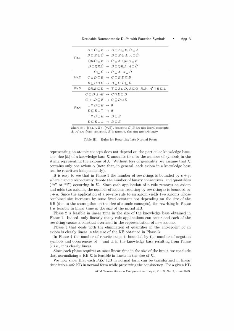
Decidable Nonmonotonic DLPs with Function Symbols · App–3
Ph.1
D ⊕ C ⊑ E D ⊕A⊑ E, C ⊑A
D ⊑ E ⊕ C D ⊑ E ⊕A, A⊑ C
QR.C ⊑ E C ⊑A, QR.A⊑ E
D ⊑ QR.C D ⊑ QR.A, A⊑ C
Ph.2
C ⊑ D C ⊑A, A⊑ D
C ⊔D ⊑B C ⊑B,D ⊑B
B ⊑ C ⊓D B ⊑ C, B ⊑D
Ph.3 QR.B ⊑D ⊤⊑A ⊔D, A⊑ Q−R.A′, A′ ⊓B ⊑⊥
Ph.4
C ⊑D ⊔ ¬E C ⊓ E ⊑D
C ⊓ ¬D ⊑ E C ⊑D ⊔ E
⊥ ⊓D ⊑ E ∅
D ⊑ E ⊔ ⊤ ∅
⊤ ⊓D ⊑ E D ⊑ E
D ⊑ E ⊔ ⊥ D ⊑ E
where ⊕ ∈ {⊓,⊔}, Q ∈ {∀,∃}, concepts C, D are not literal concepts,A, A′ are fresh concepts, B is atomic, the rest are arbitrary.
Table III. Rules for Rewriting into Normal Form
representing an atomic concept does not depend on the particular knowledge base.The size |K| of a knowledge base K amounts then to the number of symbols in thestring representing the axioms of K. Without loss of generality, we assume that Kcontains only one axiom α (note that, in general, each axiom in a knowledge basecan be rewritten independently).
It is easy to see that in Phase 1 the number of rewritings is bounded by c + q,where c and q respectively denote the number of binary connectives, and quantifiers(“∀” or “∃”) occurring in K. Since each application of a rule removes an axiomand adds two axioms, the number of axioms resulting by rewriting α is bounded byc + q. Since the application of a rewrite rule to an axiom yields two axioms whosecombined size increases by some fixed constant not depending on the size of theKB (due to the assumption on the size of atomic concepts), the rewriting in Phase1 is feasible in linear time in the size of the initial KB.
Phase 2 is feasible in linear time in the size of the knowledge base obtained inPhase 1. Indeed, only linearly many rule applications can occur and each of therewriting causes a constant overhead in the representation of new axioms.
Phase 3 that deals with the elimination of quantifier in the antecedent of anaxiom is clearly linear in the size of the KB obtained in Phase 3.
In Phase 4 the number of rewrite steps is bounded by the number of negationsymbols and occurrences of ⊤ and ⊥ in the knowledge base resulting from Phase3, i.e., it is clearly linear.
Since each phase requires at most linear time in the size of the input, we concludethat normalizing a KB K is feasible in linear in the size of K.
We now show that each ALC KB in normal form can be transformed in lineartime into a safe KB in normal form while preserving the consistency. For a given KB
ACM Transactions on Computational Logic, Vol. 9, No. 9, June 2099.

App–4 · T. Eiter and M. Simkus
K we can construct the safe knowledge base K′ by modifying K in the following way:
– for each individual name i occurring in K, adding the assertion Dom(i) to K,
– for each role R of K, adding Dom⊑ ∀R.Dom to K, and
– replacing each axiom ⊤⊑D ∈ K of type (T3), by Dom⊑D,
where Dom is a fresh concept name not occurring in K. Indeed, K′ is safe andin normal form by construction. It is easy to verify that K is consistent iff K′
is consistent. Indeed, if I is a first-order interpretation that is a model of Θ(K),then we can extend I to be a model of Θ(K′) by extending I to interpret Dom asthe whole domain of I. For the other direction, suppose K′ is consistent. SinceALC has the forest-shaped model property (cf. [Baader et al. 2003]), due to theconstruction, there exists a model I of Θ(K′) where every domain element satisfiesDom. Then, trivially, I is a model of Θ(K). The construction of K′ is clearly linearin the size of K.
A.3 Brave Entailment in FDNC
Proof of Theorem 5.13. Suppose (A) holds, i.e., there exists some I ∈ SM (P )such that A(t) ∈ I, for some term t. By Theorem 3.13, ffa(I) ∈ SM (gp(P )). LetG = ffa(I). By Proposition 3.21, K(I) is a set of knots that is founded w.r.t. P andst(G). Due to the definition of KP and Proposition 3.30, we have that KP is com-patible with st(G). It remains to show that (ii) in (B) holds. Consider reachA(K(I)).Due to the fact that A(t) ∈ I and the construction of reachA(K(I)), for some con-stant c there exists K ∈ K(I) such that st(G, c) ≈ st(K,x) and K ∈ reachA(K(I)).Due to the definition of KP , K(I) ⊆ KP . Therefore K ∈ KP . Moreover, it triviallyholds that K ∈ reachA(K(I)) implies K ∈ reachA(KP ). Therefore, (ii) holds.
Suppose (B) holds. The facts that G ∈ SM (gp(P )), and that KP is compatiblewith st(G) imply that F(G, KP ) 6= ∅ and each I ∈ F(G, KP ) is a stable modelof P (see Theorem 3.26). The condition (ii) and the construction of forest-shapedinterpretations ensure that some I ∈ F(G, KP ) contains an atom A(t), where t issome term.
Proof of Theorem 5.16. Similar to the proof of Theorem 5.13, and thus omit-ted.
A.4 Open Queries
Proof of Proposition 5.19. For the “only if” direction, suppose a groundterm t is such that P |=c A(t). Suppose c is the constant of t, and t = fn(. . . f1(c) . . .).Let t0, . . . , tn be the list of subterms of t ordered w.r.t. increasing term depth, i.e.,t0 = c and ti = fi(. . . f1(c) . . .), where i ∈ {1, . . . , n}.
Define the sequence s = [L0
c, L1
f1, . . . , Ln
fn], where Li = {K↓x | I ∈ SM (P ), K =
I ∩HBti}, for i ∈ {0, . . . , n}. We verify that s is convergent.
Since P is consistent, each Li is a nonempty subset of KP . Since P |=c A(t), thesequence s trivially satisfies the conditions (1) and (3) in Definition 5.18. Suppose(2) is not satisfied. Then there exists some j ∈ {1, . . . , n}, some K ∈ Lj−1 and someK ′ ∈ KP such that st(K, fj(x)) ≈ st(K ′,x) and K ′ 6∈ Lj . Take the smallest index jfor which the statement above holds. Then there exists a sequence K0, . . . ,Kj−1,Kj
ACM Transactions on Computational Logic, Vol. 9, No. 9, June 2099.
Decidable Nonmonotonic DLPs with Function Symbols · App–5
of knots in KP such that the sequence N = [K0
t0, . . . ,
Kj−1
tj−1,
Kj
tj] has the following
properties:
– Ki ∈ Li for each i ∈ {0, . . . , j − 1}, while Kj 6∈ Lj ;
– st(Ki, fi+1(x)) ≈ st(Ki+1,x) for each i ∈ {0, . . . , j − 1}.
Let S = st(K0,x). Due to the definition of trees, we know that there exists atree T induced by KP with root S such that N ∈ T . Consider the stable modelI ∈ SM (P ) where st(I, c) ≈ S. Such I must exists due to the way we definedL0. By the semantic characterization (see Theorem 3.34), I can be represented asI = ffa(I) ∪ (T c1)↓ ∪ . . . ∪ (T cn)↓, where {c1, . . . , cn} is the set of all constants ofP , and each T ci is a tree induced by KP with root st(ffa(I), ci). W.l.o.g., c1 = c.Simply define I ′ = ffa(I)∪ (T )↓ ∪ (T c2)↓ ∪ . . .∪ (T cn)↓. By Theorem 3.26, we havethat I ′ is also a stable model of P . We arrive at a contradiction to the assumptionthat Kj 6∈ Lj . Indeed, Kj = (I ′ ∩HBtj
)↓x
, and, due to the definition of s, Kj ∈ Lj .
For the other direction we show that the failure of (A) implies the failure of (B).Suppose for each term t, P 6|=c A(t). Furthermore, assume there exists a convergingsequence s = [L0
c, L1
f1, . . . , Ln
fn] for A, where L0 = seeds(c, P ). First, we reconstruct
the term encoded in the sequence. Let t0 = c, while tn is defined inductively asti = fi(ti−1), where 1 ≤ i ≤ n. Consider the term tn. By assumption, there existsa model I of P such that A(tn) 6∈ I. There are two possibilities.
a) ti ∈ I, for each i ∈ {0, . . . , n}. Due to the definition of KP and the fact that K(I)is founded, we have that each Ki = (HBti
∩ I)↓x is in KP , where 0 ≤ i ≤ n. Byassumption, we have K0 ∈ L0. The condition (2) in Definition 5.18 implies thatKn ∈ Ln. Since A(x) 6∈ Kn, we have that s is not a converging sequence for Adue to violation of (3) in Definition 5.18.
b) For some i, where 0 < i ≤ n, we have tiˆ6∈I. Note that t0 ∈ I since it is a constant.
Take the smallest m, where 0 ≤ m < n, such that tm+1ˆ6∈I. As it was argued,
each Ki = (HBti∩ I)↓x is in KP , where 0 ≤ i ≤ m. By assumption, we have
K0 ∈ L0. The condition (2) in Definition 5.18 implies that Km ∈ Lm. Since
Km = (HBtm∩ I)↓x and tm+1
ˆ6∈I, we have that fm(x) 6∈ succ(Km). We havethat s is not a converging sequence for A due to violation of (1) in Definition 5.18.
In both cases s is a converging sequence for A, which contradicts the assumption.
Definition A.1. A deterministic Turing machine (DTM) is a quadruple(S,Σ, δ, s0), where S is a finite set of states, Σ is a finite alphabet, δ is a tran-sition function, and so ∈ S is the initial state. The transition function δ is apartial function
δ : S × Σ→ (S ∪ {accept})× Σ× {−1, 0,+1},
where accept is a new state not occurring in S. We assume a special symbol b in Σthat stands for blank symbol. By Ik we denote the kth symbol in the input stringI = I0, . . . , I|I|−1.
Proof of Theorem 5.22 (ExpSpace-Hardness). Consider a language L overan alphabet Σ in ExpSpace. Then there is a Turing machine M = (S,Σ, δ, s0) asin Definition A.1 that decides membership of a given word I in L on a tape whose
ACM Transactions on Computational Logic, Vol. 9, No. 9, June 2099.
App–6 · T. Eiter and M. Simkus
length is bounded by an exponential in the size of I. We construct a FD programP (M, I) of size polynomial in M and I such that acceptance of I by M is equivalentto the existence of an answer for an open query λx.A(x) under cautious entailment.
For convenience, we assume here that I is not the empty word. Suppose thenumber of cells (the space) used by M on the input I is bounded by m = 2as, whereas is polynomial in the size of I. The reduction relies on keeping two addressesof the cells in the work tape, each of which is represented using as = log2 m bits.The first address is the position of the read/write (r/w) head, which is encodedby the unary predicate symbols rwposb
0, . . ., rwposbas, b ∈ {0, 1}. For each bit of
the address, we dedicate two symbols and will ensure that exactly one of themholds for each term. In our encoding, terms will represent stages reached in thecomputation of the machine on some path. Similarly, the second address is the oneof the observed cell, which is encoded by the unary predicate symbol oposb
0, . . . ,oposb
as, b ∈ {0, 1}. Intuitively, the observed cell is the single cell of the machinefor which the correct state transition will be ensured by the program. By non-deterministically generating all cells for observation in parallel, and exploiting theproperties of cautious entailment of open queries we will ensure that acceptingcomputations of M (represented by terms) can be singled out.
We sketch the construction of the program P (M, I) in steps. We need rules forchecking the equality of the r/w head address and the address of the observed cell.To this end, for a bit b, let b = 1−b denote the complement of b. For the comparisonof separate bits in the two addresses, we add the following rule
equi(x)← oposbi (x), rwposb
i (x) for all i ∈ {0, . . . , as} and b ∈ {0, 1}. (2)
The equality of two addresses at some point of computation is then expressed easilyby the rule
rwoequ(x)← equ0(x), . . . , equas(x). (3)
The inequality is also easily expressed by the rules
nonequ(x)← oposbi (x), rwposb
i (x) (4)
for all i ∈ {0, . . . , as} and b ∈ {0, 1}.We move to the representation of the initial configuration of the machine, which
we do from the perspective of an observed cell. To this end, we add, for 0 ≤ i ≤ as,the facts
rwpos0i (st)← , (5)
states0(st)← , (6)
opos1i (st) ∨ opos0
i (st)← . (7)
Intuitively, (5) sets the position of the r/w head to the left most cell and (6) set themachine into the start state, while (7) non-deterministically chooses an observedcell of the tape. To represent the content of each observed cells in the initialconfiguration, we proceed as follows.
For each symbol α ∈ Σ, we use a designated unary predicate symbol symbolα.Let n ≥ 0 be the position of the last symbol of I written on the tape, i.e., I =I0I1 · · · In is on positions 0,. . . ,n. For each position i ≤ n with binary representation
ACM Transactions on Computational Logic, Vol. 9, No. 9, June 2099.

Decidable Nonmonotonic DLPs with Function Symbols · App–7
i = b0 · · · bas = i and α = Ii, we add the rule
symbolα(st)← oposb00 (st), . . . , oposbas
as (st). (8)
For all other positions, the symbols are blank. Assuming that n = b∗0 · · · b∗as in
binary, we express this with rules
symbolb(st)← oposb∗11 (x), . . . , opos
b∗j−1
j−1 (x), opos1j (x), (9)
for all j ∈ {0 . . . , as} such that b∗j = 0.
This describes the initial configuration; note that it is captured by the whole setof models for the program described so far. Although each model captures only thecontent of one (the observed) cell, the contents of the whole work tape is entirelycaptured as the addresses of the observed cells cover the whole work space of M .
To encode the transitions, it is handy to view δ as a table. For each tuplet = 〈s, α, s′, α′,D〉 such that δ(s, α) = 〈s′, α′,D〉, we use a function symbol t anddefine the following rules:
next(x, t(x))← rwoequ(x), states(x), symbolα(x), (10)
next(x, t(x))←nonequ(x), states(x), (11)
states′(t(x))←next(x, t(x)), (12)
symbolα′(t(x))← rwoequ(x), next(x, t(x)), (13)
moveD(t(x))←next(x, t(x)). (14)
The rules above are explained as follows. If the r/w head is at the position ofthe observed cell, and the symbol and the state are correct for the transition, thetransition is made (10). If the r/w head is not at the position of the observedcell, the transition is made blindly (11). The single case where the transition isnot made is if the r/w head is at the position of the observed cell, but either thesymbol or the state is not the right one. The rule (12) sets the new state, while(13) sets the new symbol of the observed cell. The rule (14) triggers the movementof the r/w head. The effect of moveD is explained next. Moving the r/w head boilsdown to adding or subtracting one bit from the address. To this end, we use unarypredicates shiftb0,. . ., shiftbas, b ∈ {0, 1}, to simulate the values of the carry bit.When the r/w head position changes, the last bit should be inverted. This is statedby the rules
shift1as(x)←move+1(x), (15)
shift1as(x)←move−1(x), (16)
shift0as(x)←move0(x). (17)
The position of r/w head after shifting is then defined by the following rules for
ACM Transactions on Computational Logic, Vol. 9, No. 9, June 2099.

App–8 · T. Eiter and M. Simkus
each j ∈ {0, . . . , as}, j′ ∈ {1, . . . , as}, and b ∈ {0, 1}:
rwposbj(y)← shift1j (y), rwposb
j(x), next(x, y), (18)
rwposbj(y)← shift0j (y), rwposb
j(x), next(x, y), (19)
shiftbj′−1(y)←move+1(y), shift1j′(y), rwposbj′(x), next(x, y), (20)
shiftbj′−1(y)←move−1(y), shift1j′(y), rwposbj′(x), next(x, y), (21)
shift0j (x)←move0(x). (22)
Furthermore, we have to state that the address of the observed cell does not change,i.e., is fixed for a model. This expressed by the rules
oposbi (y)← oposb
i (x), next(x, y), (23)
for each i ∈ {0, . . . , as} and b ∈ {0, 1}. Finally, we ensure that the symbol writtenin the observed cell does not change if it is not affected by the transition. This isexpressed by the following inertia rule for each α ∈ Σ:
symbolα(y)← nonequ(x), symbolα(x), next(x, y). (24)
This completes the description of the program P (M, I). It is not hard to seethat P (M, I) has exactly m = 2as minimal models (and thus stable models, as inP (M, I) no negation occurs) that are induced by different choices of the positionof the observed cell. Let R0, . . . , Rm−1 be these models ordered with respect to theposition of the observed cell, i.e., R0 is the one for first position 0 while Rm−1 isthe one for the last position m− 1.
Without loss of generality, we view a run of M on an input I as a sequencet1, . . . , tn of transitions, and assume that it is always non-empty. The run is ac-cepting, if after performing tn, the machine enters the accepting state accept. Weestablish the following lemmas.
Lemma A.2. If the machine M accepts the input I on the run t1, . . . , tn, n ≥ 1,then P (M, I) |=c stateaccept(u), where u = tn(. . . t1(st) . . .).
Proof. Suppose that I0 = Ib · · · b is the word describing the initial tape con-tents, and that after executing the transitions t1, . . . , ti, (i) Ii is the word given bythe tape contents, (ii) si is the state of the machine, and (iii) posi is the positionof the r/w head.
We show that for each Rw, w ∈ {0, . . . ,m − 1}, we have stateaccept(u) ∈ Rw.To this end, we show that in Rw the content of the observed cell w, the state,and the r/w head position are correctly reflected through the computation. Moreformally, let u0 = st, and ui = ti(ui−1), where 0 < i ≤ n. Then we argue that,for each j ∈ {0, . . . , n}, (i) symbolα(uj) ∈ Rw whenever α = Ij
w, i.e., α is writtenin cell w, (ii) statesj
(uj) ∈ Rw, and (iii) posj is, encoded, in binary, by the atomsrwposb
i (uj) ∈ Rw, 0 ≤ i ≤ as. Note that this will prove the lemma, since sn =accept.
We proceed by induction on j ≥ 0. The base case j = 0 is clear by the encodingof the initial word (rules (8) and (9)), the initial r/w head position (facts (5)) andthe initial state (fact (6)).
ACM Transactions on Computational Logic, Vol. 9, No. 9, June 2099.

Decidable Nonmonotonic DLPs with Function Symbols · App–9
For the inductive case, assume the claim holds for 0 ≤ j < n and consider j + 1.By the induction hypothesis, symbolα(ui) ∈ Rw, statesj
(uj) ∈ Rw, and posj isdescribed by the atoms rwposb
i (uj) ∈ Rw. There are now, by the rules (2) – (4)two disjoint cases: either nonequ(uj) ∈ Rw or rwoequ(uj) ∈ Rw. In the formercase, next(uj , tj+1(uj)) ∈ Rw by the rule (11); by the rule (24), we then havesymbolα(uj+1) ∈ Rw. In the latter case, next(uj , tj+1(uj)) ∈ Rw by the rule (10);by the rule (13), we then have symbolα′(uj+1) ∈ Rw. In both cases, Rw containssymbolα(uj+1) where Ii+1
w = α. Hence (i) holds for j + 1.As for (ii), as we have next(uj , tj+1(uj)) ∈ Rw, by the rule (12) we have
statesi+1(ui+1) ∈ Rw, and thus (ii) holds for j + 1. Finally, the rules (14) and
(15) – (22) effect that atoms posbi (uj+1) which correctly represent posj+1 are de-
rived. Hence, (iii) holds for j + 1.
Lemma A.3. If P (M, I) |=c λx.stateaccept(x), then there exists an accepting runof M .
Proof. Suppose P (M, I) |=c stateaccept(u). By assumption, the initial stateis not accept and thus u = tn(. . . t1(st) . . .), where n ≥ 1. Let u0 = st, andui = ti(ui−1), where 0 < i ≤ n. Then, in each model Rw, we must clearly musthave next(ui−1, ti(ui−1)) for each 0 < i ≤ n (otherwise, stateaccept(un) would notbe contained in Rw).
For each i ∈ {0, . . . , n}, define (i) the word Ii = α0 · · ·αm−1 where αj is such thatsymbolαj
(ui) ∈ Rj , 0 ≤ j < m, (ii) si as the state s such that states(ui) ∈ Rw, and
(iii) posi as the integer which, in binary, is encoded by the facts rwposbi
i (uj) ∈ Rw,i.e., posi = b0 · · · bas, where w ∈ {0, . . . ,m− 1} is arbitrary.
We claim that each Ii, si, and posi is well-defined and is the tape contents, state,and r/w head position, respectively, after the partial run t1, . . . , ti of M on theinput I. Since sn = accept, this will prove the lemma.
The proof is by induction on i ≥ 0. For the base case i = 0, by construction,I0 clearly is the initial tape contents, s0 = s0, and pos0 = 0 by the facts and rules(5) – (9). Suppose the claim holds for 0 ≤ i < n and consider i + 1. Assumeti+1 = 〈s, α, s′α′,D〉. Since we have next(ui, ti+1(ui)) in each Rw, we must havestates′(ui+1) in Rw by rule (12); since no other fact states′′(ui+1) can be in Rw,si+1 is well-defined. Furthermore, we must have states(ui) in Rw and either (a)rwoequ(ui) ∈ Rw or (b) nonequ(ui) ∈ Rw; by the induction hypothesis and therules (2) – (4), (a) is the case if posi = w and (b) if posi 6= w. In case (a), wemust have symbolα(ui) ∈ Rw and symbolα′(ui+1) ∈ Rw by rule (13), and in case(b) symbolα(ui+1) ∈ Rw by rule (24), where symbolα(ui) ∈ Rw. Since no otherfacts symbolα′′(ui+1) can be in Rw, Ii+1 is well-defined. Finally, we must havemoveD(ui+1) in Rw by rule (14); by the induction hypothesis and the rules (15) –
(22), we have facts rwposbj
j (ui+1) in Rw, 0 ≤ j ≤ as, such that b0, . . . , bas represents
posi + D = posi+1 in binary.Summing up, Ii+1, s+1, and posi+1 are all well-defined and encode tape contents,
state, and r/w head position, respectively, after the partial run t1, . . . , ti+1 of Mon the input I, which concludes the induction step.
As P (M, I) and λx.stateaccept(x) are constructible in polynomial time from Mand I, from Lemmas A.2 and A.3 the claimed ExpSpace-hardness result follows
ACM Transactions on Computational Logic, Vol. 9, No. 9, June 2099.
App–10 · T. Eiter and M. Simkus
for FD, FDN, and FDNC; by replacing the disjunctive guessing rules (7) with un-stratified rules opos1
i (st) ← not opos0i (st); opos0
i (st) ← not opos1i (st), we obtain
the result for FN and FNC.
A.5 Reasoning in FN
Proof of Proposition 6.2. Let I be a stable model of fr(P ). The properties(1), (2) and (3) hold by the construction of fr(P ), i.e., due to the fact that I is astable model that satisfies (F1)-(F4) rules of fr(P ). Suppose I does not satisfy (4),i.e., for some term t ∈ I and some unary predicate A of P , either (a) {A(t), A(t)} ∩I = ∅, or (b) {A(t), A(t)} ⊆ I. In case (a), we have {A(t) ← Dom(t); A(t) ←Dom(t)} ⊆ fr(P )I . Since Dom(t) ∈ I, I is not a model of fr(P )I . In case (b), byconstruction of fr(P ), there is no rule in fr(P )I that has head A(t) or A(t), andhence I is not a minimal model of fr(P )I . In both cases, we arrive to a contradictionto the assumption that I is a stable model of fr(P ). Analogously to the argumentfor (4), one can show that the property (5) holds.
For the other direction, assume an interpretation I of fr(P ) for which the givenproperties hold. It is easy to see that such an interpretation satisfies each of therules in fr(P )I . We verify that I is a minimal model of fr(P )I . By the constructionof fr(P ), each minimal model of fr(P ) has to satisfy (1), (2) and (3). Therefore, ifI is not a minimal model of fr(P )I , there should exists a model H ⊂ I of fr(P )I forwhich (4) or (5) does not hold. We arrive to a contradiction. Due to the rules oftypes (F5-F8) in fr(P ), H cannot be a model of fr(P )I .
Proof of Proposition 6.4. Suppose P is consistent, and I is a minimal modelof P . We know that I is forest-shaped. Let J be a Herbrand interpretation fortf(P ) defined as the smallest set of atoms satisfying the following conditions:
a) I ⊆ J ,
b) S(c, d) ∈ J , for each pair c, d of constants of P ,
c) if t ∈ J , then Dom(t) ∈ J ,
d) if t ∈ J and f is a function symbol of P , then S(t, f(t)) ∈ J ,
e) if t ∈ J and A(t) 6∈ J , then A(t) ∈ J , and
f) if S(s, t) ∈ I and R(s, t) 6∈ I, then R(s, t) ∈ J ,
where A and R are predicate symbols of P . We show that J is a stable model oftf(P ). Assume that it is not the case. There are two possibilities.
1) J is not a model of tf(P )J . Since fr(P ) ⊆ tf(P ), we have fr(P )J ⊆ tf(P )J . Fromthe construction of J it follows that J is a model of fr(P )J . Then tf(P )J mustcontain some ground rule
C(~v1)← Q1(~v1), . . . , Qm(~vm), W1(~t1), . . . , Wn(~tn)
such that (⋆) {Q1(~v1), . . . , Qm(~vm), W1(~t1), . . . , Wn(~tn)} ⊆ J and C(~v1) 6∈ J . Byconstruction, P contains the rule W1(~t1)∨ . . .∨Wn(~tn)← Q1(~v1), . . . , Qm(~vm),where n,m ≥ 0. Since I is a model of P , then either (a) {Q1(~v1), . . . , Qm(~vm)} 6⊆I or (b) {W1(~t1), . . . ,Wn(~tn)} ∩ I 6= ∅. In case (a), by the definition of J , (⋆)does not hold. In case (b), for some Wi(~ti) of the rule, Wi(~ti) 6∈ J and, hence,(⋆) does not hold.
ACM Transactions on Computational Logic, Vol. 9, No. 9, June 2099.

Decidable Nonmonotonic DLPs with Function Symbols · App–11
Generating time:
T ime(st)←N(x, f(x))← T ime(x)
T ime(y)← N(x, y)
Initial configuration:
Symα,π(st)← for 0 ≤ π < |I| such that α = Iπ
Symb,π(st)← for |I| ≤ π ≤ sb(I)
Cur0(st)←Sts0
(st)←
Transition δ(s, σ) = 〈s′, σ′, d〉, where 0 ≤ π ≤ sb(I)
Symσ′,π(y)← N(x, y), Sts(x), Symσ,π(x), Curπ(x)
Sts′ (y)← N(x, y), Sts(x), Symσ,π(x), Curπ(x)Curπ+d(y)← N(x, y), Sts(x), Symσ,π(x), Curπ(x)
Inertia rules, where 0 ≤ π < π′ ≤ sb(I):
Symσ,π(y)← N(x, y), Symσ,π(x), Curπ′(x)
Symσ,π′ (y)← N(x, y), Symσ,π′ (x), Curπ(x)
Table IV. FC program P (T, I) for simulating a DTM T on input I.
2) J is a model but is not a minimal model of tf(P )J . Since fr(P ) ⊆ tf(P ), wehave fr(P )J ⊆ tf(P )J . Then we also have that J is a model of fr(P )J , but is not
minimal. However, by construction of J , we have J ⊆ HBfr(P ) and J satisfiesthe conditions in Proposition 6.2, and hence by the same proposition, J mustbe a minimal model of fr(P )J . Contradiction.
For the other direction, let I ∈ SM (tf(P )). Let J be the restriction of I to thepredicates of P . Suppose J 6|= P . Then Ground(P ) contains a rule
W1(~t1) ∨ . . . ∨Wn(~tn)← Q1(~v1), . . . , Qm(~vm),
where n,m ≥ 0, such that {Q1(~v1), . . . , Qm(~vm)} ⊆ J and {W1(~t1), . . . ,Wn(~tn)} ∩J = ∅. By construction, Ground(tf(P )) contains
r = C(~t1)← Q1(~v1), . . . , Qm(~vm), W1(~t1), . . . , Wn(~tn), not C(~t1).
By hypothesis, I ∈ SM (tf(P )). Clearly, C(t1) 6∈ I (otherwise, I /∈ MM (tf(P )I)as no rule in tf(P )I would have C(t1) in the head). Hence, tf(P )I contains therule resulting from r by removing not C(~t1). Since {Q1(~v1), . . . , Qm(~vm)} ⊆ I andI |= tf(P )I , it follows that Wi(~ti) 6∈ I for some i ∈ {1, . . . , n}. As I is forest-shaped, by the rules in fr(P ) we have Wi(~ti) ∈ I, and thus Wi(~ti) ∈ J . However,this contradicts that {W1(~t1), . . . ,Wn(~tn)} ∩ J = ∅.
A.6 Reasoning in FC
Lemma A.4. Deciding whether a given FC program is consistent is PSpace-hard.
Proof. Let L be a language in PSpace, and let T be a DTM which decideswhether a given word I is in L within space sb(I) that is polynomial in |I|. Thecomputation of T on I can be simulated by an F program P (T, I) (see Table A.6).Due to construction, we can use a single constraint to decide whether I ∈ L. It iseasy to see that I ∈ L iff P (T, I) ∪ {← Staccept(x)} is inconsistent.
As the translation is clearly polynomial in the size of T and I, deciding I ∈ L isreducible in polynomial time to consistency checking of an FC program.
ACM Transactions on Computational Logic, Vol. 9, No. 9, June 2099.

App–12 · T. Eiter and M. Simkus
A.7 Reasoning in F and FD
Proof of Theorem 6.16. If (i) holds, then, due to Theorem 3.13, we can easilydefine G and L such that the conditions in (ii) are satisfied. On the other hand, if(ii) is satisfied, the fact that for each G ∈ MM (gp(P )) there is some M ∈ MM (P )such that G = ffa(M) and Theorem 3.13 imply that a minimal model of P suchthat A(t) ∈ P for some term t is constructible. Indeed, take some M for G asdescribed. By Theorem 3.13, M is forest-shaped. As L is founded w.r.t. P and{st(G, c)}, the tree in M rooted at c can be replaced by some tree that is built withinstances of knots from L only, and such that some instance of a knot K containingA(x) is used. As the resulting model I is forest-shaped, by Theorem 3.13 we obtainthat I ∈ SM (P ).
Lemma A.5. For F programs, brave entailment of unary existential queries isPSpace-hard.
Proof. Recall the program P (T, I) in Table A.6 that simulates a computationof a DTM T on input I. Note that it is an F program and has size polynomial in thesize of T and I. To check whether T accepts I, we can pose the brave query whetherStaccept(t) is in the minimal model of P (T, I) for some term t, i.e., T accepts I iffP (T, I) |=b ∃x.Staccept(x).
Proof of Proposition 6.19. For the only-if direction of the first claim, as-sume we have a stable model I of P such that A(t) ∈ I. Due to Theorem 3.13,we can simply define G = ffa(I) and Ki = HBsi
∩ I, where 1 ≤ i ≤ n. Forthe if direction, since for FD programs each G ∈ SM (gp(P )) is extendible to someM ∈ SM (P ), we can similarly as in the proof of Theorem 6.16 construct using The-orem 3.13 a stable model of P containing A(sn); simply start with G∪K1∪ . . .∪Kn
and extend the set with the necessary stable knots.For the only-if direction of the second claim, the argument is as for the first
claim. If I ∈ SM (P ) such that A(t) 6∈ I, then, by Theorem 3.13, we can easilydefine G and the sequence of knots. Again, take G = ffa(I) and Ki = HBsi
∩ I,where 1 ≤ i ≤ n. For the if direction, let I be the unique stable model of P . LetK ′
i = HBsi∩ I, where 1 ≤ i ≤ n. Due to Theorem 3.13, we have Ic ⊆ G and
K ′i ⊆ Ki, where 1 ≤ i ≤ n. Hence, A(sn) 6∈ I.
B. APPLICATION: REASONING ABOUT ACTIONS AND PLANNING
In Section 5, we have already encountered an application of FDNC programs toDescription Logics. In this section, we consider a further application of FDNC
programs in the area of reasoning about actions and planning; recall that non-monotonic logic programs under answer set semantics have been widely used inthis area. In particular, we apply FDNC programs to planning under incompleteknowledge and non-deterministic action effects, based on the expressive action lan-guage K [Eiter et al. 2004].
Transition-based action formalisms are based on languages for describing legaltransitions between states of the world which happen due to the execution of actionsby some agent. A classical problem is that of plan existence, which consists offinding a sequence of actions that leads the agent from an initial to some desiredgoal state of the world. Apart from this, many problems have been considered,
ACM Transactions on Computational Logic, Vol. 9, No. 9, June 2099.

Decidable Nonmonotonic DLPs with Function Symbols · App–13
including plan verification (i.e., whether a given candidate plan is good to reach agoal state) and temporal projection (i.e., reasoning about the hypothetical future ifa sequence of action would be taken); as for the concerns of this paper, we refer to[Baral 2002] for background and a study of these problems based on logic programsunder answer set semantics.
As for temporal projection in Example 3.2, view grow , cell1, cell2, and die asactions and Young , Warm, Cold , and Mature as fluents. As seen, if the sequenceof actions grow and cell1 would happen, the fluent Young would be possibly true,as Young(cell1(grow(b))) is bravely entailed by the program. On the other hand,Young is not necessarily true after this action sequence. Indeed, using similarlyas in Proposition 6.13 an auxiliary fact C0(b). and rules R(x, grow(x)) ← C0(x);C1(y)← C0(x), R(x, y); R(x, cell1(x))← C1(x); and ← R(x, y), not Change(x, y),we can eliminate those stable models of P ex which do not correspond to the oc-currence of this sequence; the resulting program P ′ does not cautiously entailYoung(cell1(grow(b))), as it has a stable model which does not contain this atom.In this scenario, planning seems not to make sense (as bacteria can’t really takeactions), and we thus consider a different one.
For modeling planning domains, several dedicated action languages have beenproposed that are rooted in knowledge representation formalisms, including A[Gelfond and Lifschitz 1992] (which was extensively studied in [Baral 2002]), C[Giunchiglia and Lifschitz 1998], and K [Eiter et al. 2004]. The latter, which weconsider in the sequel, is based on the principles of logic programming under thestable model semantics. In contrast to the other languages, K allows to describetransitions between knowledge states, which are incompletely described states ofthe world. The availability of non-monotonic negation in K makes the formalismsuitable for common-sense and heuristic reasoning in planning applications.
In K, a planning domain PD is a set of rules that describes the initial state Iand legal transitions.6 At the core, it distinguishes two kinds of predicates: fluentsand actions. A state is given by a set of ground fluent literals which are known tohold at a particular stage. A goal G is a set of ground fluent literals, each of whichcan also be default negated.
An optimistic (or credulous) plan for a given planning domain PD and a goalG is a sequence of action occurrences 〈A1, . . . ,An〉, n ≥ 0, that legally transformsthe initial state I into some state that satisfies the goal G, i.e., for some sequenceof states, we have (i) S0 = I, (ii) each Si,Ai+1, Si+1 is a legal transition, and (iii)Sn satisfies G. For our concerns, Ai is a single action.
In case of non-deterministic action effects or incomplete information about theinitial state, executing an optimistic plan does not necessarily establish the goal.This is ensured by secure plans (also known as conformant plans), which are op-timistic plans such that, regardless of such incompleteness and non-deterministic
6We consider here merely a simplified version of K that contains the salient elements; missingfeatures like static predicates, typing and others can be added easily on top. Furthermore, we as-sume that actions are not executed in parallel (parallel execution may be encoded using designatedaction symbols), that at each stage some action has to be taken to move on (thus passage of time
would have to be modeled explicitly by an action), and that taking an executable action alwaysresults in a follow up state. Technically, such planning domains are proper and more general thanplain ones in the sense of [Eiter et al. 2004].
ACM Transactions on Computational Logic, Vol. 9, No. 9, June 2099.

App–14 · T. Eiter and M. Simkus
action effects, all actions can be executed and the goal is established after the lastaction.
The legal state transitions are defined in K in terms of stable model semantics.Roughly speaking, this is accomplished using a set of statements, similar to logicprogram rules, which describe the value of the fluents in the successor state S′
depending on the previous state S, the action A that was taken, and the thevalue of other fluents in S′. Because of this similarity, planning problems in Kcan be naturally encoded into FDNC programs. Via such encodings, optimistic andsecure plan existence can be characterized in terms of brave entailment of existentialqueries and cautious entailment of open queries, respectively.
More in detail, we consider here the propositional fragment of K, i.e., predicatesare nullary (predicates of higher arity will be addressed in the next subsection). Aplanning domain PD in K consists of causation rules, executability conditions, andinitial state constraints. The causation rules of propositional K are of the form
caused D if B1, . . . , Bn, not Bn+1, . . . , not Bk
after C1, . . . , Cm, not Cm+1, . . . , not Cl
A1, . . . , Av, not Av+1, . . . , not Aw
(25)
k, l, w ≥ 0, where d and B1, . . . , Bk, C1, . . . , Cl are fluent literals, and A1, . . . , Aw
are action atoms. Intuitively, the rule (25) describes the (incomplete) knowledgestate after action execution, where the knowledge depends on fluents that hold(C1, . . . , Cm) and do not hold (Cm+1, . . . , Cl) in the old state, fluents that hold(B1, . . . , Bn) and do not hold (Bn+1, . . . , Bk) in the new state, and actions that wereexecuted (A1, . . . , Av) respectively were not executed (Av+1, . . . , Aw) in parallel.7
The executability conditions in K are of the form
executable A if B1, . . . , Bn, not Bn+1, . . . , not Bk,A1, . . . , Am, not Am+1, . . . , not Al,
(26)
where A,A1, . . . , Al are action atoms, and B1, . . . , Bk are fluent literals, k, l ≥ 0,Intuitively, they are the rules constraining the states for which a given action canbe executed.
The initial state constraints in K are of the form
initially caused D if B1, . . . , Bn, not Bn+1, . . . , not Bk (27)
where D,B1, . . . , Bk are fluent literals, k ≥ 0. These rules describe the initialknowledge. Unconditional initial knowledge is described by the rules with an emptyif part.
We next sketch the elements of a possible encoding of the planning domain PDinto an FDNC program. As in Section 7, we enhance FDNC programs with “strong”negation ¬P (~x) [Gelfond and Lifschitz 1991], which is expressed in the core languageas usual.
—For each propositional fluent symbol d, we use a unary predicate symbol d in theencoding. The meaning of d(x) is that d holds at stage x. For each propositionalaction a, we use a binary predicate symbol a in the encoding. Intuitively, a(x, y)means that a is executed in stage x with the resulting stage y.
7For our concerns, we may restrict to v ≤ 1.
ACM Transactions on Computational Logic, Vol. 9, No. 9, June 2099.

Decidable Nonmonotonic DLPs with Function Symbols · App–15
—We use a unary predicate symbol S, with S(x) meaning that x is a stage (ora situation). For the encoding we add the fact S(init) ← denoting that theconstant init is the initial stage. We also use a designated binary predicatesymbol tr to denote the transition to the next stage. For this reason, we also addS(y)← Tr(x, y).
—We adopt a function symbol fA for each action A of the planning domain. Addi-tionally, for each action A, we add the rule a(x, fA(x))← ExecA(x) and the ruleTr(x, y)← a(x, y), whereexeca is a designated predicate name. Intuitively, the first rule “implements”the action execution, i.e., if Execa holds at some stage x, then a is executed,which results in the follow up stage fa(x). The second rule makes Tr capture allexecuted transitions.
We can now state the encoding of the three types of rules of the planning domainPD.
—The causation rule (25) is transformed into the following rule:
D(y)← B1(y), . . . , Bn(y), not Bn+1(y), . . . , not Bk(y),C1(x), . . . , Cm(x), not Cm+1(x), . . . , not Cl(x),A1(x, y), . . . , Av(x, y), not Av+1(x, y), . . . , not Aw(x, y), T r(x, y)
—The executability condition (26) is transformed into the following rule:
Execa(y)← S(y), B1(y), . . . , Bn(y), not Bn+1(y), . . . , not Bk(y),A1(x, y), . . . , Av(x, y), not Av+1(x, y), . . . , not Aw(x, y).
Here, we assume for simplicity as in [Eiter et al. 2003] that there are no positivecyclic interdependencies between actions.
—The initial state constraint (27) is transformed into the following rule:
d(init)← B1(init), . . . , Bn(init), not Bn+1(init), . . . , not Bk(init),
The translation above allows to reformulate planning problems in PD as reasoningtasks for FDNC programs. A goal G in PD is an expression of the form
G1, . . . , Gn, not Gn+1, . . . , not Gk (28)
where each Gi is a fluent literal. For this, we add to the translation the followingrule:
Plan(x)← G1(x), . . . , Gn(x), not Gn+1(x), . . . , not Gk(x) (29)
where Plan is a new predicate symbol. Let P (PD,G) denote the resulting program.To know whether an optimistic plan for G in PD exists, we can pose the brave
query ∃x.Plan(x) to the program P (PD,G). Similarly, the cautious open queryλx.Plan(x) can be posed for a secure plan. Due to the stable model semanticsof both languages, it is not hard (yet technical) to show that a stable modelof P (PD,G) encodes a set of possible trajectories S0,A1, S1,A2, . . . in PD, i.e.,alternating sequences of states Si and action occurrences Ai+1 such that eachSi,Ai+1, Si+1 is a legal transition, 0 ≤ i < n, where S0 is any initial knowledgestate; the whole set SM (P (PD,G)) captures all the trajectories for PD.
ACM Transactions on Computational Logic, Vol. 9, No. 9, June 2099.

App–16 · T. Eiter and M. Simkus
Further, each term t such that P (PD,G) |=b Plan(t) naturally encodes an op-timistic plan for the problem, and each term t that is an answer for λx.Plan(x)under cautious entailment encodes a secure plan. Thus, plan correctness and se-curity verification problems can be readily solved by the standard inference tasksP (PD,G) |=b Plan(t) and P (PD,G) |=c Plan(t).
We note at this point that deciding the existence of some secure plan (of arbitrarylength) to establish a given goal G in a given K action domain that conforms tothe setting considered here is ExpSpace-complete (this is well-known for a genericrelated action formalism [Haslum and Jonsson 1999]; the hardness part can beshown by slightly adapting the NExpTime-hardness proof for the problem when aprescribed plan length is part of the input [Eiter et al. 2004]).
Finally, also temporal projection with respect to an action sequence ~A = A1, A2,. . . , Ak, k ≥ 1, can be easily expressed: whether a fluent D is possibly true afterhypothetically taking ~A is expressed by the entailment P (PD) |=b d(t) where t =fAk
(fAk−1· · · (fA1
(init))) where P (PD) is P (PD,G) except the rules (28) and (29).
Whether D is necessarily true when ~A would have happened can be expressed, usingagain a similar technique as in Proposition 6.13, as cautious entailment of D(t) fromP (D) augmented with the auxiliary fact C0(init)← and rules
R(x, fAi+1(x)) ← Ci(x), for 0 ≤ i < k,
Ci+1(y) ← Ci(x), R(x, y), for 0 ≤ i < k − 1,
← R(x, y), not Tr(x, y),
where all Ci and R are fresh predicates (this singles out the models in which ~awould be taken).
Further tasks like reasoning about the initial state or observation assimilation[Baral 2002] can be similarly expressed.
Example B.1. Table V presents an example encoding of a propositional plan-ning domain in K into an FDN program P , which is an adaptation of the classicalYale-Shooting example [Hanks and McDermott 1987]. Here we assume three flu-ents See, Loaded, Hit, and two actions load and shoot. In the initial situation,a hunter sees a target, but his gun is not loaded (row (1)). The fluents See andLoaded are inertial, i.e., their truth values do not change unless proved otherwise(rows (2) and (3)). The hunter can load the gun only if it is unloaded, and canshoot only if the gun is loaded (rows (4) and (5)). The gun becomes loaded afterloading occurs (row(6)). Finally, the hunter hits the target, if he shoots while seeingthe target (row (7)). The goal in the planning domain is Hit, and hence the rulePlan(x)← Hit(x) is added to the encoding.
It is easy to see that P |=b ∃x.Plan(x), i.e., there exists a plan where the hunterhits the target and is witnessed by the term t = shoot(load(init)). The inertia ofSee is crucial; dropping the statement in row (3) wouldn’t let us assume that thehunter still sees the target after loading the gun.
The term t also encodes a secure plan for the domain, i.e., t witnesses the openquery λx.Plan(x). This becomes false when instead of sure knowledge that the gunis not loaded in the initial state, the status of the gun in the initial stage can varyfreely. This situation is modeled by the two rules caused Loaded if not ¬Loadedand caused ¬Loaded if not Loaded. In this case, t is still an optimistic plan for
ACM Transactions on Computational Logic, Vol. 9, No. 9, June 2099.

Decidable Nonmonotonic DLPs with Function Symbols · App–17
(1) initially caused See,¬Loaded
See(init)←;
¬Loaded(init)←;
(2) caused Loaded if not ¬Loaded after Loaded
Loaded(y)← Loaded(x), T r(x, y), not ¬Loaded(y)
(3) caused See if not ¬See after See
See(y)← See(x), T r(x, y), not ¬See(y)
(4) executable load if ¬Loaded
Execload(x)← ¬Loaded(x)
(5) executable shoot if Loaded
Execshoot(x)← Loaded(x)
(6) caused Loaded after load
Loaded(y)← load(x, y), T r(x, y)
(7) caused Hit after See, shoot
Hit(y)← See(x, y), shoot(x, y), T r(x, y)
Table V. Example of Planning Domain Encoding (mapping via )
the domain, but is not secure (as the first step might not be executable). On theother hand, if hypothetically t would happen, then Hit would be both possibly andnecessarily true after it.
To provide a procedure for deciding plan existence in the planning domains ofK, the authors of [Eiter et al. 2004] encode the domain into a disjunctive Datalogprogram and reformulate plan existence in terms of brave entailment. Since Datalogdoes not allow for function symbols, the encoding uses constants to instantiate thenecessary successor stages. Obviously, only a finite number of constants can be usedand hence, it has to be fixed in advance. For this reason the encoding is not general;only plans of certain length can be captured. Furthermore, such an encoding mayalso incur high space requirements.
The encoding into FDNC solves the problems from above. The availability offunction symbols allows to easily generate an infinite time-line, and, hence, to avoidthe usage of constants. Due to the properties of FDNC, the encoding also allows togenerate the successors states “on-demand” during the model construction; in thisway, space might be saved.
We remark that using higher arity FDNC, we can represent the Yale-Shootingscenario alternatively using a generic predicate holds(f, x) to express truth of thefluent f in a situation x, where f is reified using a constant symbol, in the styleof [Baral 2002]; e.g., holds(Loaded , init) corresponds then to Loaded(init). Furtherpredicates, e.g. abnormal(f, x), can be used to express other aspects of fluents.While the syntax of FDNC does not allow reification of fluents with parameters,e.g. on(A,B) to holds(on(A,B), x), which is also used [Baral 2002], this can beeasily accommodated with tailored predicates, e.g. holdson(A,B, x); on the otherhand, an extension of the syntax of FDNC programs that allows such terms in localpositions is easily accomplished, and does not affect the worst case complexity.
ACM Transactions on Computational Logic, Vol. 9, No. 9, June 2099.