Fault Detection for Robot Manipulators via Second-Order Sliding Modes

3954 IEEE TRANSACTIONS ON INDUSTRIAL ELECTRONICS, VOL. 55, NO. 11, NOVEMBER 2008

Fault Detection for Robot Manipulators viaSecond-Order Sliding Modes

Daniele Brambilla, Luca Massimiliano Capisani, Member, IEEE, Antonella Ferrara, Senior Member, IEEE,and Pierluigi Pisu, Member, IEEE

Abstract—This paper presents a model-based fault detection(FD) and isolation scheme for rigid manipulators. A single faultacting on a specific actuator or on a specific sensor of the manip-ulator is detected (and, if possible, the exact location of the fault),and an estimation of the fault signal is performed. Input-signalestimator and output observers are considered in order to makethe FD procedure possible. By using the suboptimal second-ordersliding-mode (SOSM) algorithm to design the input laws of theobservers, satisfactory stability properties of the observation errorare established. The proposed algorithm is verified in simulationand experimentally on a COMAU SMART3-S2 robot manipulator.

Index Terms—Fault diagnosis, fault location, manipulators,robustness, variable structure systems.

I. INTRODUCTION

IN ACTUAL automatically controlled systems, faults canoccur both on the mechanical and on the electrical part of the

plant [1]–[4]. The capability of detecting a fault in a small timeinterval enables one to reduce the probability of damages orcritical injuries to the people who operate around the controlledsystem.

Faults are modeled as unknown input signals acting on thesystem. In electromechanical systems like robots, a single faultcan occur on a specific actuator, on a specific sensor, or ona specific component of the system. The actuator and sensorfaults are more frequent because of the presence of electricaldevices and connections. Fault detection (FD) techniques aim togenerate diagnostic signals that are sensitive to the occurrenceof faults, while fault isolation allows one to locate the inputrelated to the fault from all the other system inputs and togenerate a specific residual signal for each fault. A necessaryand sufficient condition for the fault isolation problem to besolvable is the existence of an unobservability subspace leadingto a quotient subsystem unaffected by all fault signals apartfrom one [5], [6].

Often, residual generators for dynamical systems are basedon unknown input or output observers [7]–[9]. The so-calledgeneralized momenta approach [10] consists in an input ob-

Manuscript received January 29, 2008; revised August 21, 2008. Currentversion published October 31, 2008.

D. Brambilla is with the Ente Nazionale Idrocarburi (ENI) Research Institute,20097 Milan, Italy (e-mail: [email protected]).

L. M. Capisani and A. Ferrara are with the Department of Computersand Systems Science, University of Pavia, 27100 Pavia, Italy (e-mail: [email protected]; [email protected]).

P. Pisu is with the Department of Mechanical Engineering, Clemson Univer-sity, Clemson, SC 29634 USA (e-mail: [email protected]).

Color versions of one or more of the figures in this paper are available onlineat http://ieeexplore.ieee.org.

Digital Object Identifier 10.1109/TIE.2008.2005932

server for actuator faults which does not require an estimationof the accelerations and of the inverse of the inertia matrix. Thedetection of sensor faults is a challenging problem because ofthe presence, in the system, of unmodeled effects, which canmake particularly critical the state observation and prediction.In [11], a discrete time observer has been proposed, which isable to predict the system noise relying on the measurements atthe previous sampling instants.

Sliding-mode observers have been exploited in two possibleways. In the first case, the FD procedure is performed when thesliding condition is corrupted [12], while in the second case,the fault reconstruction is accomplished by combining multiplesliding-mode observers [13]–[15].

In this paper, an FD scheme for rigid robot manipulators ispresented. It is based on the inverse dynamics approach (see [7]and [16]) to make the fault detection and identification (FDI) ofan actuator fault possible and, on a generalized observer scheme(GOS) (see [8]), to detect a sensor fault. To ensure robustness,the input law of each GOS observer is determined relying ona second-order sliding-mode (SOSM) law of sub-optimal type[17], [18]. In this way, a second-order sliding manifold can bereached in finite time in spite of the uncertainties, guaranteeingthe asymptotic convergence to zero of the observation error.Note that because of the GOS structure, only a single sensorfault can be detected at a time, while the actuator faults can alsobe multiple. Sufficient conditions are given to make the faultisolation possible.

This paper has the following structure. In Section II, themodel of the manipulator is presented, while Sections III and IVdescribe the proposed FD scheme. Finally, in Sections V–VII,simulations (based on the model of a real COMAU SMART3-S2 robot) and experimental results (made directly on this robot)are reported.

II. MANIPULATOR MODEL

Advanced FDI schemes are based on the model of thesystem, in order to provide analytical redundancy, which isuseful to compare the inputs and the outputs of the faulty systemwith those predicted by the model. The dynamics of a fault-freen-joint manipulator is described in the joint space, by using theLagrangian approach, as

τ = B(q)q + n(q, q) n(·) = C(q, q)q + g(q) + Fv q (1)

(see [16]) where q = [q1, . . . , qn]T ∈ Rn is the vector of joint

displacements, τ ∈ Rn is the vector of motor control torques,

B(q) ∈ Rn×n is the known inertia matrix, C(q, q)q ∈ R

n

0278-0046/$25.00 © 2008 IEEE

BRAMBILLA et al.: FAULT DETECTION FOR ROBOT MANIPULATORS VIA SECOND-ORDER SLIDING MODES 3955

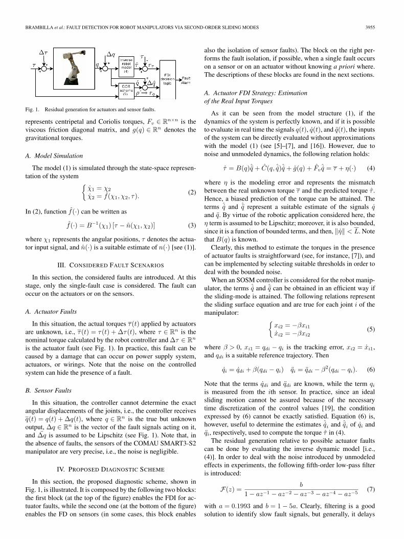
Fig. 1. Residual generation for actuators and sensor faults.

represents centripetal and Coriolis torques, Fv ∈ Rn×n is the

viscous friction diagonal matrix, and g(q) ∈ Rn denotes the

gravitational torques.

A. Model Simulation

The model (1) is simulated through the state-space represen-tation of the system {

χ1 = χ2

χ2 = f(χ1, χ2, τ). (2)

In (2), function f(·) can be written as

f(·) = B−1(χ1) [τ − n(χ1, χ2)] (3)

where χ1 represents the angular positions, τ denotes the actua-tor input signal, and n(·) is a suitable estimate of n(·) [see (1)].

III. CONSIDERED FAULT SCENARIOS

In this section, the considered faults are introduced. At thisstage, only the single-fault case is considered. The fault canoccur on the actuators or on the sensors.

A. Actuator Faults

In this situation, the actual torques τ(t) applied by actuatorsare unknown, i.e., τ(t) = τ(t) + Δτ(t), where τ ∈ R

n is thenominal torque calculated by the robot controller and Δτ ∈ R

n

is the actuator fault (see Fig. 1). In practice, this fault can becaused by a damage that can occur on power supply system,actuators, or wirings. Note that the noise on the controlledsystem can hide the presence of a fault.

B. Sensor Faults

In this situation, the controller cannot determine the exactangular displacements of the joints, i.e., the controller receivesq(t) = q(t) + Δq(t), where q ∈ R

n is the true but unknownoutput, Δq ∈ R

n is the vector of the fault signals acting on it,and Δq is assumed to be Lipschitz (see Fig. 1). Note that, inthe absence of faults, the sensors of the COMAU SMART3-S2manipulator are very precise, i.e., the noise is negligible.

IV. PROPOSED DIAGNOSTIC SCHEME

In this section, the proposed diagnostic scheme, shown inFig. 1, is illustrated. It is composed by the following two blocks:the first block (at the top of the figure) enables the FDI for ac-tuator faults, while the second one (at the bottom of the figure)enables the FD on sensors (in some cases, this block enables

also the isolation of sensor faults). The block on the right per-forms the fault isolation, if possible, when a single fault occurson a sensor or on an actuator without knowing a priori where.The descriptions of these blocks are found in the next sections.

A. Actuator FDI Strategy: Estimationof the Real Input Torques

As it can be seen from the model structure (1), if thedynamics of the system is perfectly known, and if it is possibleto evaluate in real time the signals q(t), q(t), and q(t), the inputsof the system can be directly evaluated without approximationswith the model (1) (see [5]–[7], and [16]). However, due tonoise and unmodeled dynamics, the following relation holds:

τ = B(q)ˆq + C(q, ˆq)ˆq + g(q) + Fvˆq = τ + η(·) (4)

where η is the modeling error and represents the mismatchbetween the real unknown torque τ and the predicted torque τ .Hence, a biased prediction of the torque can be attained. Theterms ˆq and ˆq represent a suitable estimate of the signals qand q. By virtue of the robotic application considered here, theη term is assumed to be Lipschitz; moreover, it is also bounded,since it is a function of bounded terms, and then, ‖η‖ < L. Notethat B(q) is known.

Clearly, this method to estimate the torques in the presenceof actuator faults is straightforward (see, for instance, [7]), andcan be implemented by selecting suitable thresholds in order todeal with the bounded noise.

When an SOSM controller is considered for the robot manip-ulator, the terms ˆq and ˆq can be obtained in an efficient way ifthe sliding-mode is attained. The following relations representthe sliding surface equation and are true for each joint i of themanipulator: {

xi2 = −βxi1

xi2 = −βxi2(5)

where β > 0, xi1 = qdi − qi is the tracking error, xi2 = xi1,and qdi is a suitable reference trajectory. Then

qi = qdi + β(qdi − qi) qi = qdi − β2(qdi − qi). (6)

Note that the terms qdi and qdi are known, while the term qi

is measured from the ith sensor. In practice, since an idealsliding motion cannot be assured because of the necessarytime discretization of the control values [19], the conditionexpressed by (6) cannot be exactly satisfied. Equation (6) is,however, useful to determine the estimates ˆqi and ˆqi of qi andqi, respectively, used to compute the torque τ in (4).

The residual generation relative to possible actuator faultscan be done by evaluating the inverse dynamic model [i.e.,(4)]. In order to deal with the noise introduced by unmodeledeffects in experiments, the following fifth-order low-pass filteris introduced:

F(z) =b

1 − az−1 − az−2 − az−3 − az−4 − az−5(7)

with a = 0.1993 and b = 1 − 5a. Clearly, filtering is a goodsolution to identify slow fault signals, but generally, it delays


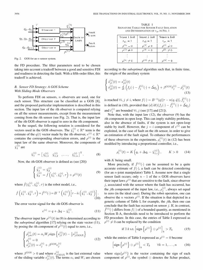
Fig. 2. GOS for an n-sensor system.

the FD procedure. The filter parameters need to be chosentaking into account a tradeoff between a good and sensitive FDIand readiness in detecting the fault. With a fifth-order filter, thistradeoff is achieved.

B. Sensor FD Strategy: A GOS SchemeWith Sliding-Mode Observers

To perform FDI on sensors, n observers are used, one foreach sensor. This structure can be classified as a GOS [8],and the proposed particular implementation is described in thissection. The input law of the ith observer is computed relyingon all the sensor measurements, except from the measurementcoming from the ith sensor (see Fig. 2). That is, the input lawof the ith GOS observer is equal to zero in the ith component.

In the sequel, the following notation is considered for thevectors used in the GOS observers. The χ

(i)1 ∈ R

n term is theestimate of the q(t) vector made by the ith observer, e(i) ∈ R

n

contains the corresponding observation errors, and ρ(i) is theinput law of the same observer. Moreover, the components ofχ

(i)1 are

χ(i)1 =

[χ

(i)1,1 χ

(i)1,2 , . . . , χ

(i)1,n

]T. (8)

Now, the ith GOS observer is defined as (see [20])⎧⎨⎩

˙χ(i)

1 = χ(i)2

˙χ(i)

2 = f(χ

(i)1 , χ

(i)2 , τ

)+ ρ(i)(t)

(9)

where f(χ(i)1 , χ

(i)2 , τ) is the robot model, i.e.,

f(χ

(i)1 , χ

(i)2 , τ

)= f (i)(·)=B−1

(χ

(i)1

)[τ−n

(χ

(i)1 , χ

(i)2

)].

(10)

The error vector signal for the ith GOS observer is

e(i) = q + Δq − χ(i)1 . (11)

The observer input law ρ(i)(t) in (9) is determined according tothe suboptimal algorithm [17] relying on the state vector (11),by posing the ith component of ρ(i)(t) equal to zero, i.e.,⎧⎪⎪⎨

⎪⎪⎩ρ(i)j �=i(t) = αjWjsign

{s(i)j1 (t) − 1

2s(i)j1MAX

}ρ(i)i = 0

s(i)j1 (t) = e

(i)j + βGOSe

(i)j

(12)

where βGOS > 0 and where s(i)j1MAX is the last extremal value

of the sliding variable s(i)j1 (t). The terms αi and Wi are chosen

TABLE ISIGNATURE TABLE FOR SENSOR FAULT ISOLATION

AND DETERMINATION OF rqi IN FIG. 1

according to the suboptimal algorithm such that, in finite time,the origin of the auxiliary system⎧⎨⎩

s(i)j1 (t) = s

(i)j2 (t)

s(i)j2 (t) = d

dt

(fj(·) − f

(i)j (·) + Δqj

)+ βGOS e

(i)j − ρ

(i)j (t)

(13)

is reached ∀i, j �= i, where f(·) = B−1(q)[τ − n(q, q)], f(i)j (·)

is defined in (10), provided that (d/dt)(fj(·) − f(i)j (·) + Δqj)

and e(i)j are bounded ∀i, j (see [17] and [21]).

Note that, with the input law (12), the observer (9) has theith component in open loop. This can imply stability problems,also in the absence of faults, if the system is not open-loopstable by itself. However, the j = i component of e(i) can beexploited, in the case of fault on the ith sensor, in order to givean estimation of the fault signal. To enhance the performancesof these observers in the experiments, ρ

(i)i (t) in (12) has been

modified by introducing a proportional controller, i.e.,

ρ(i)i (t) = K

(qi + Δqi − χ

(i)1,i

), K > 0 (14)

with K being small.More precisely, if f (i)(·) can be assumed to be a quite

accurate estimate of f(·), a fault can be detected considering(for an n-joint manipulator) Table I. Assume now that a singlesensor fault occurs; only n − 1 of the n GOS observers havetheir input laws ρ(i) that are sensitive to the fault, since observerj, associated with the sensor where the fault has occurred, hasthe jth component of the input law, i.e., ρ

(j)j , always set equal

to zero (in the ideal case). During the robot operation, one canobserve the n vectors ρ(i). If the situation is that depicted in ageneric column of Table I, for example, the jth, then one canconclude that the fault has occurred on sensor j. If, in contrast,f (i)(·) differs from f(·) of a bounded quantity, as mentioned inSection II-A, thresholds need to be introduced to perform theFD procedure. In this case, the entries of Table I expressed asρ(i) �= 0 can be replaced by the condition

if ∃ k s.t.[sign

{ρ(i)

}� ρ(i)

]k

> Tk (15)

while the entries of Table I expressed as ρ(i) = 0 become[sign

{ρ(i)

}� ρ(i)

]k

< Tk ∀k = 1, . . . , n (16)

where sign{ρ(i)} is the vector containing the sign of eachcomponent of ρ(i), the symbol � denotes the Schur product,


[·]k denotes the kth component of a vector, and Tk is a positivereal number representing the selected threshold. The thresholdsdepend on the magnitude of the uncertain term B−1(q)η.Obviously, now the fact that a fault has occurred on sensorj can be inferred when (15) is true ∀i �= j and (16) is truefor i = j.

Remark 1: Note that no useful information can be obtainedby analyzing the terms e

(i)j , j �= i because of the asymptotic

motions imposed by sliding-mode control.Remark 2: Each observer of the conventional GOS scheme

is generally defined to have an input law that is linearly de-pendent on the observation error [8]. Yet, in this way, it is notpossible to ensure exact tracking of the n − 1 measured signals,and this fact can lead to a reduction of the performances of thesensor FD.

C. Residual Generation

Fig. 1 shows the complete diagnostic scheme for robotmanipulators. The τ vector signal represents the estimation ofthe torques obtained via the inverse dynamics, (4) by applyingthe filter (7), while q is defined as

q =[χ

(1)1,1 χ

(2)1,2 · · · χ

(n)1,n

]T(17)

and represents an estimate of q(t) (obtained relying on theopen-loop components of each observer). However, note thatto consider the q term does not make sense to identify the faultwhen the modified input law (14) is adopted.

The residual vector rτ is given by

rτ i ={

0, if |τi − τi| < Tτ i

1, if |τi − τi| > Tτ i∀i (18)

while rq is obtained evaluating Table I. To choose suitablethresholds, tuning experiments need to be executed.

D. Error Signature Table

Now, consider the case in which a single fault occurs, but onedoes not know where. To isolate the fault means to determine ifthe fault has occurred on the actuators or on the sensors.

Unfortunately, a sensor fault can affect the actuator faultresiduals and vice versa, possibly leading to a wrong faultisolation. However, for a small fault on sensors, i.e., for smallΔq, and for small velocities and accelerations of the robotmanipulator system, one has that the actuator residual signal rτ

is not sensitive to a sensor fault Δq if B(q + Δq)ˆq − B(q)q +n(q + Δq, ˆq) − n(q, q) is less than the actuator fault threshold.In fact, this term represents an estimation of the mismatchbetween the predicted torque and the torque generated by theactuators.

After one has obtained the rτi and the rqi vectors, the iso-lation of a fault can be done by making a comparison with thefault signature Table II. One can conclude that a fault is presenton sensor i if only one of the residuals referred to the sensorsis equal to 1 and if all the residuals referred to the actuatorsare equal to 0 or at least two of them are equal to 1. One can

TABLE IIFAULT SIGNATURE TABLE, WHERE p REPRESENTS

A VALUE THAT CAN BE 0 OR 1

conclude that a fault is present on the actuator i when the dualholds. Since an actuator fault can produce nonzero residuals rq

on the sensors and a sensor fault can produce nonzero residualsrτ on the actuators, the p values in Table II can be 0 or 1, andin general, a single fault cannot be isolated if the fault inducesthe detection of one actuator fault and one sensor fault. Notethat, during transient phases when accelerations and speeds arenot low, the fault isolation may be challenging, while FD isalways possible. This issue is further clarified by the followingtheorem.

Theorem 1: Under the assumptions of single fault, of exactknowledge of the manipulator model, and of the absence ofnoise on sensor measurements, a sensor fault Δq can beisolated from an actuator fault if the following conditions hold.

1) The n-degrees-of-freedom manipulator belongs to a ver-tical plane, and each link has a nonnull gravitationalcontribution on each actuator.

2) The sensor fault signal Δq is time invariant, i.e.,Δq = Δq = 0.

3) The robot manipulator represented by the model (1) is instatic work conditions, i.e., q = q = 0.

In particular, when a single fault acts on a specified componentof vector q, the former conditions assure that it is impossibleto detect a nonexistent single fault on Δτ (no false alarms canoccur).

Proof: Under the assumption of a single-fault presence,of the absence of noise, and of the exact knowledge of themanipulator model, the only situation in which it is not possibleto establish where the fault has occurred is that of a singlefault which is detected both as an actuator and as a sensorfault. A wrong measurement made by a position sensor due toa fault presence generally gives a wrong estimation of the inputtorques [see (4)]

τ = B(q + Δq)q + n(q + Δq, q + Δq) (19)

so it is necessary to avoid the situation in which one and onlyone component of the τ vector differs from the given inputvector τ , which is exactly known due to the assumption thatthe only fault is on sensors. The input-torque estimator (19)with the former assumptions reduces to τ = n(q + Δq, q) =g(q + Δq), where

g(q + Δq) = [g1(·), g2(·), . . . , gn(·)]T . (20)


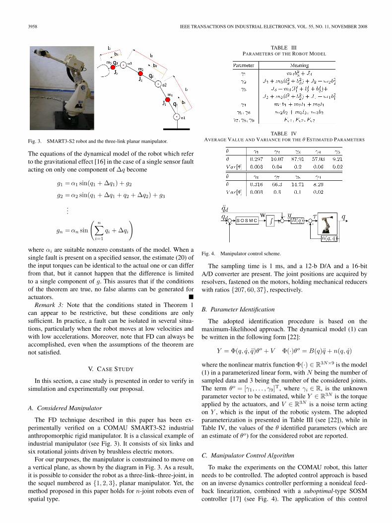
Fig. 3. SMART3-S2 robot and the three-link planar manipulator.

The equations of the dynamical model of the robot which referto the gravitational effect [16] in the case of a single sensor faultacting on only one component of Δq become

g1 =α1 sin(q1 + Δq1) + g2

g2 =α2 sin(q1 + Δq1 + q2 + Δq2) + g3

...

gn =αn sin

(n∑

i=1

qi + Δqi

)

where αi are suitable nonzero constants of the model. When asingle fault is present on a specified sensor, the estimate (20) ofthe input torques can be identical to the actual one or can differfrom that, but it cannot happen that the difference is limitedto a single component of g. This assures that if the conditionsof the theorem are true, no false alarms can be generated foractuators. �

Remark 3: Note that the conditions stated in Theorem 1can appear to be restrictive, but these conditions are onlysufficient. In practice, a fault can be isolated in several situa-tions, particularly when the robot moves at low velocities andwith low accelerations. Moreover, note that FD can always beaccomplished, even when the assumptions of the theorem arenot satisfied.

V. CASE STUDY

In this section, a case study is presented in order to verify insimulation and experimentally our proposal.

A. Considered Manipulator

The FD technique described in this paper has been ex-perimentally verified on a COMAU SMART3-S2 industrialanthropomorphic rigid manipulator. It is a classical example ofindustrial manipulator (see Fig. 3). It consists of six links andsix rotational joints driven by brushless electric motors.

For our purposes, the manipulator is constrained to move ona vertical plane, as shown by the diagram in Fig. 3. As a result,it is possible to consider the robot as a three-link–three-joint, inthe sequel numbered as {1, 2, 3}, planar manipulator. Yet, themethod proposed in this paper holds for n-joint robots even ofspatial type.

TABLE IIIPARAMETERS OF THE ROBOT MODEL

TABLE IVAVERAGE VALUE AND VARIANCE FOR THE θ ESTIMATED PARAMETERS

Fig. 4. Manipulator control scheme.

The sampling time is 1 ms, and a 12-b D/A and a 16-bitA/D converter are present. The joint positions are acquired byresolvers, fastened on the motors, holding mechanical reducerswith ratios {207, 60, 37}, respectively.

B. Parameter Identification

The adopted identification procedure is based on themaximum-likelihood approach. The dynamical model (1) canbe written in the following form [22]:

Y = Φ(q, q, q)θo + V Φ(·)θo = B(q)q + n(q, q)

where the nonlinear matrix function Φ(·) ∈ R3N×9 is the model

(1) in a parameterized linear form, with N being the number ofsampled data and 3 being the number of the considered joints.The term θo = [γ1, . . . , γ9]T, where γi ∈ R, is the unknownparameter vector to be estimated, while Y ∈ R

3N is the torqueapplied by the actuators, and V ∈ R

3N is a noise term actingon Y , which is the input of the robotic system. The adoptedparameterization is presented in Table III (see [22]), while inTable IV, the values of the θ identified parameters (which arean estimate of θo) for the considered robot are reported.

C. Manipulator Control Algorithm

To make the experiments on the COMAU robot, this latterneeds to be controlled. The adopted control approach is basedon an inverse dynamics controller performing a nonideal feed-back linearization, combined with a suboptimal-type SOSMcontroller [17] (see Fig. 4). The application of this control


scheme to a COMAU SMART3-S2 manipulator has been de-scribed in [18] and [21]. Here follows a brief outline of thecontrol approach.

1) Inverse Dynamics Part of the Control Scheme: Bychoosing a control law of the form

τ = B(q)y + n(q, q) = Φ(q, q, y)θo (21)

system (1) simply becomes q = y. Note that, even if the termn(q, q) in (21) has been accurately identified, it can be quite dif-ferent from the real one because of uncertainties and unmodeleddynamics, friction, and joint plays. The n(q, q) term containsthe identified centripetal, Coriolis, gravity, and friction torqueterms, while the inertia matrix B(q) is known. Thus, letting

τ = B(q)y + n(q, q) = Φ(q, q, y)θ (22)

where θ is identified, the compensated system becomes

q(t)=y(t)−ε, ε=−B−1 (n(·)−n(·))=B−1η (23)

where ε(·) ∈ R3 is the modeling error, which is Lipschitz,

by virtue of the assumption of the Lipschitzianity of η.2) SOSM Part of the Control Scheme: Relying on (23), the

control objective is to steer to zero the error state vector

xi(t) =[xi1(t)xi2(t)

]=

[qd(t) − q(t)

xi1(t)

](24)

where xi1(t) = qdi(t) − qi(t), qd is the reference signal, qd andqd exist and are bounded, while i = {1, 2, 3} represents thejoint considered. In this case, a suitable sliding manifold canbe chosen as

si = s(xi) = x2i + βx1i ∀i, β = 10. (25)

In the particular case of the SOSM, the controller aim is tosteer to zero in a finite time the sliding variable s = [s1, s2, s3]T

and its first time derivative s. Indeed, in this way, a chatteringreduction is achieved because the control signal is continuous.

A particular SOSM technique is the suboptimal algorithm.To design the suboptimal control law, an auxiliary state vectorcan be introduced, i.e.,

ξi = [ξi1, ξi2]T = [si, si]T (26)

where s is defined in (25). Then, taking into account (23) and(24), the following auxiliary system can be formulated for eachjoint i: ⎧⎪⎨

⎪⎩ξi1(t) = ξi2(t)ξi2(t) = εi − yi(t) + d3qdi(t)

dt3 + βxi2(t)yi(t) = wi(t) + d3qdi(t)

dt3 + βxi2(t)(27)

where wi(t) is regarded as an auxiliary control signal. Since theuncertain term εi(·), i=1, 2, 3 is assumed to be Lipschitz, then,according to [17], the control signal wi(t) can be designed as

wi(t) = αiGisign

{ξi1(t) −

12ξi1MAX

}(28)

where Gi > 0, αi is chosen as indicated in [17], and ξi1MAX isthe last extremal value of ξi1. The term Gi can be determined

through an experimental tuning procedure. From a theoreticalpoint of view, if |εi(·)| < F i, it can be proved that, by choosing

Gi > max(

F i

α∗ ;4F i

3 − α∗

)(29)

and α∗ as in [17], (G = [230, 1330, 10220] and α∗ = 0.9 inour case), the state vector (26) is steered to zero in a finitetime, i.e., an SOSM is enforced, thus steering to zero s and s.Note that, as desired, the actual control signal acting on joint i,namely, yi(t), is continuous, thus attaining the requirement oflimiting the possible generation of vibrations. Also, the tuningof the controller parameters is done experimentally. Therefore,a precise estimation of F i is not necessary.

VI. SIMULATION RESULTS

In the next two sections, the performances of the proposedFDI scheme are evaluated considering a three-link planar ma-nipulator, first by simulating three possible actuator faults, andthen by simulating a possible sensor fault. Note that noise isadded on the considered actuator and sensor signals in order tomake the simulations.

To perform the simulations, the system (2) has been consid-ered with the parameters obtained by applying the identificationprocedure [22] to the actual industrial robot, which are listedin Tables III and IV (the B(q) and the n(q, q) terms can beobtained from the θ parameters listed in Tables III and IV).

Note that, in simulation, the local small gain loop (14) onthe ith component of the ith observer of the GOS structureis not necessary because of the absence of unmodeled effects.This allows one to use the ith component of the vector χ

(i)1 to

identify the fault, so that our proposal, in simulation, can beregarded as an FDI scheme.

A. Actuator FD and Identification

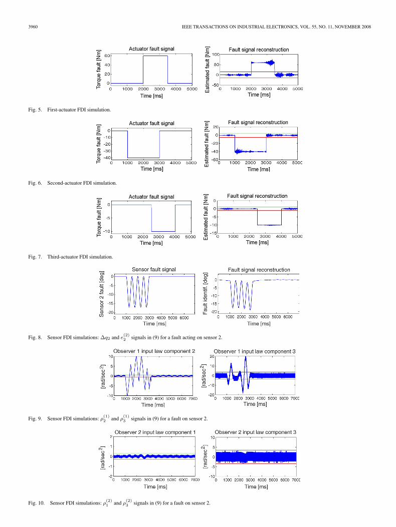
In order to simulate an actuator fault, we considered thepresence of abrupt faults Δτ on the actuators: As we can seefrom Figs. 5–7, the fault amplitude is correctly identified.

B. Sensor FDI

A simulation of the presence of a single sinusoidal sensorfault on the second joint sensor is presented in this section. Thisfault is sporadic. It appears at time instant 1 s and disappears attime instant 3 s (see Fig. 8).

Figs. 9–11 show the two components of the input laws of thethree GOS observers (9) that are not null [the third component isclearly equal to zero, as imposed by (12)]. In particular, the faultisolation can be done considering the first and the third observerinput signals (see Figs. 9 and 11), in which it is clearly observedthat the relative thresholds are exceeded, while, as expected, theinput laws of the second observer are not affected by the fault.Therefore, it is possible to establish that the fault has occurredon the second sensor. The identification of the fault signal isshown in Fig. 8. Note that some high-frequency noise has beenadded to the actuator torque signals, as previously mentioned.Fixed thresholds have been defined to detect the fault.


Fig. 5. First-actuator FDI simulation.

Fig. 6. Second-actuator FDI simulation.

Fig. 7. Third-actuator FDI simulation.

Fig. 8. Sensor FDI simulations: Δq2 and e(2)2 signals in (9) for a fault acting on sensor 2.

Fig. 9. Sensor FDI simulations: ρ(1)2 and ρ

(1)3 signals in (9) for a fault on sensor 2.






Fig. 12. FDI experiment on the first actuator.

Fig. 13. FDI experiment on the third actuator.

VII. EXPERIMENTAL RESULTS

In this section, the proposed scheme is experimentally tested.The faults are introduced by adding a Δτ signal to the τ signal(in the case of actuator fault) or a Δq signal to the q signal(in the case of sensor fault). In this case, noise and unmodelednonlinear effects are naturally present.

A. Experimental FDI of Actuators

Experiments dealing with actuator faults have been de-veloped through the introduction of abrupt faults on the joints,whose values are Δτ1 = 50 N · m on the first actuator andΔτ3 = 10 N · m on the third one, respectively.

As it can be seen from Figs. 12 and 13, the faults are correctlyidentified after a short time interval.

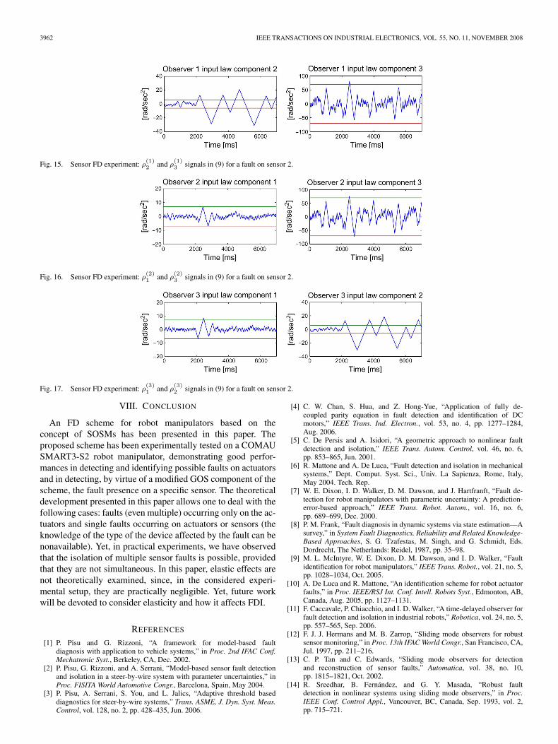
B. Experimental FD and Isolation of Sensor Faults

As for the sensors, in the experimental case, the presence ofnonlinear and unmodeled effects leads to a corruption of thesignals useful for the fault analysis. To reduce this effect, eachGOS observer has been modified to enhance its relative stability[see (14)]. The following experiment is performed: An abruptfault of Δq2 = 60◦ on the second joint sensor measurement isintroduced starting from time instant 2 s (Fig. 14). To isolatethe joint affected by the fault, the proposed fault signature table(Table II) is considered. Figs. 15–17 show the two components

Fig. 14. Sensor FD experiment: Δq2 signal for a fault on sensor 2.

of the input laws different from zero of the three GOS observers(9). The fault isolation can be accomplished by considering thefirst and the third observer signals, since only these signals(in particular one of their components) exceed the thresholds.Therefore, one can conclude that the fault has occurred onsensor 2.

C. Advantages of Using the Suboptimal Algorithm

By virtue of the robustness properties of the suboptimalcontroller, the presence of a fault on actuators can be neglectedif this fault can be considered as an input noise satisfyingcondition (29). Therefore, the applied control can be regardedas a fault-tolerant control for small faults. Moreover, to usethe suboptimal algorithm to design the input law of the GOSobservers may enable a more reliable sensor FD (and isolationin some cases), since the risk of false alarms due to trackinginaccuracies is reduced.


Fig. 15. Sensor FD experiment: ρ(1)2 and ρ






VIII. CONCLUSION

An FD scheme for robot manipulators based on theconcept of SOSMs has been presented in this paper. Theproposed scheme has been experimentally tested on a COMAUSMART3-S2 robot manipulator, demonstrating good perfor-mances in detecting and identifying possible faults on actuatorsand in detecting, by virtue of a modified GOS component of thescheme, the fault presence on a specific sensor. The theoreticaldevelopment presented in this paper allows one to deal with thefollowing cases: faults (even multiple) occurring only on the ac-tuators and single faults occurring on actuators or sensors (theknowledge of the type of the device affected by the fault can benonavailable). Yet, in practical experiments, we have observedthat the isolation of multiple sensor faults is possible, providedthat they are not simultaneous. In this paper, elastic effects arenot theoretically examined, since, in the considered experi-mental setup, they are practically negligible. Yet, future workwill be devoted to consider elasticity and how it affects FDI.

REFERENCES

[1] P. Pisu and G. Rizzoni, “A framework for model-based faultdiagnosis with application to vehicle systems,” in Proc. 2nd IFAC Conf.Mechatronic Syst., Berkeley, CA, Dec. 2002.

[2] P. Pisu, G. Rizzoni, and A. Serrani, “Model-based sensor fault detectionand isolation in a steer-by-wire system with parameter uncertainties,” inProc. FISITA World Automotive Congr., Barcelona, Spain, May 2004.

[3] P. Pisu, A. Serrani, S. You, and L. Jalics, “Adaptive threshold baseddiagnostics for steer-by-wire systems,” Trans. ASME, J. Dyn. Syst. Meas.Control, vol. 128, no. 2, pp. 428–435, Jun. 2006.

[4] C. W. Chan, S. Hua, and Z. Hong-Yue, “Application of fully de-coupled parity equation in fault detection and identification of DCmotors,” IEEE Trans. Ind. Electron., vol. 53, no. 4, pp. 1277–1284,Aug. 2006.

[5] C. De Persis and A. Isidori, “A geometric approach to nonlinear faultdetection and isolation,” IEEE Trans. Autom. Control, vol. 46, no. 6,pp. 853–865, Jun. 2001.

[6] R. Mattone and A. De Luca, “Fault detection and isolation in mechanicalsystems,” Dept. Comput. Syst. Sci., Univ. La Sapienza, Rome, Italy,May 2004. Tech. Rep.

[7] W. E. Dixon, I. D. Walker, D. M. Dawson, and J. Hartfranft, “Fault de-tection for robot manipulators with parametric uncertainty: A prediction-error-based approach,” IEEE Trans. Robot. Autom., vol. 16, no. 6,pp. 689–699, Dec. 2000.

[8] P. M. Frank, “Fault diagnosis in dynamic systems via state estimation—Asurvey,” in System Fault Diagnostics, Reliability and Related Knowledge-Based Approaches, S. G. Tzafestas, M. Singh, and G. Schmidt, Eds.Dordrecht, The Netherlands: Reidel, 1987, pp. 35–98.

[9] M. L. McIntyre, W. E. Dixon, D. M. Dawson, and I. D. Walker, “Faultidentification for robot manipulators,” IEEE Trans. Robot., vol. 21, no. 5,pp. 1028–1034, Oct. 2005.

[10] A. De Luca and R. Mattone, “An identification scheme for robot actuatorfaults,” in Proc. IEEE/RSJ Int. Conf. Intell. Robots Syst., Edmonton, AB,Canada, Aug. 2005, pp. 1127–1131.

[11] F. Caccavale, P. Chiacchio, and I. D. Walker, “A time-delayed observer forfault detection and isolation in industrial robots,” Robotica, vol. 24, no. 5,pp. 557–565, Sep. 2006.

[12] F. J. J. Hermans and M. B. Zarrop, “Sliding mode observers for robustsensor monitoring,” in Proc. 13th IFAC World Congr., San Francisco, CA,Jul. 1997, pp. 211–216.

[13] C. P. Tan and C. Edwards, “Sliding mode observers for detectionand reconstruction of sensor faults,” Automatica, vol. 38, no. 10,pp. 1815–1821, Oct. 2002.

[14] R. Sreedhar, B. Fernández, and G. Y. Masada, “Robust faultdetection in nonlinear systems using sliding mode observers,” in Proc.IEEE Conf. Control Appl., Vancouver, BC, Canada, Sep. 1993, vol. 2,pp. 715–721.


[15] W. Chen and M. Saif, “Robust fault detection and isolation in constrainednonlinear systems via a second order sliding mode observer,” in Proc.15th IFAC World Congr., Barcelona, Spain, Jul. 2002, pp. 1498–1500.

[16] L. Sciavicco and B. Siciliano, Modelling and Control of RobotManipulators, 2nd ed. London, U.K.: Springer-Verlag, 2000.

[17] G. Bartolini, A. Ferrara, and E. Usai, “Chattering avoidance by second-order sliding mode control,” IEEE Trans. Autom. Control, vol. 43, no. 2,pp. 241–246, Feb. 1998.

[18] L. M. Capisani, A. Ferrara, and L. Magnani, “Design and experimentalvalidation of a second order sliding-mode motion controller for robotmanipulators,” Int. J. Control, 2007, to be published.

[19] V. I. Utkin, Sliding Modes in Control and Optimization. Moscow,Russia: Springer-Verlag, 1992.

[20] J. Davila, L. Fridman, and A. Levant, “Second-order sliding-modeobserver for mechanical systems,” IEEE Trans. Autom. Control, vol. 50,no. 11, pp. 1785–1789, Nov. 2005.

[21] L. M. Capisani, A. Ferrara, and L. Magnani, “Second order sliding modemotion control of rigid robot manipulators,” in Proc. 46th IEEE Conf.Decision Control, New Orleans, LA, Dec. 2007, pp. 3691–3696.

[22] L. M. Capisani, A. Ferrara, and L. Magnani, “MIMO identificationwith optimal experiment design for rigid robot manipulators,” in Proc.IEEE/ASME Int. Conf. Adv. Intell. Mechatron., Zürich, Switzerland,Sep. 2007, pp. 1–6.

Daniele Brambilla received the Laurea degree(cum laude) in computer science engineering fromthe University of Pavia, Pavia, Italy, in 2008.

He is currently with the “Ente NazionaleIdrocarburi” (ENI) Research Institute, Milan, Italy.His activity includes the applicability of faultdetection, isolation, and identification algorithms toexperimental systems.

Luca Massimiliano Capisani (S’06–M’06) re-ceived the Laurea degree (cum laude) in computerscience engineering from the University of Pavia,Pavia, Italy, in 2006, where he is currently workingtoward the Ph.D. degree in electronics, computerscience, and electrical engineering in the Departmentof Computers and Systems Science.

His research activities include modeling, robustsliding-mode control, planar planning, and faultdetection and isolation for robot manipulators. Hehas authored or coauthored eight papers, two journal

papers, and an international scientific book chapter.

Antonella Ferrara (S’86–M’88–SM’03) receivedthe Laurea degree in electronic engineering and thePh.D. degree in computer science and electronicsfrom the University of Genova, Genoa, Italy, in 1987and 1992, respectively.

She was an Assistant Professor with the Universityof Genova beginning in 1992. In 1998, she becamean Associate Professor at the University of Pavia,Pavia, Italy, where she has been a Full Professor ofautomatic control since January 2005. Her researchactivities include sliding-mode control with applica-

tion to automotive control, process control, and robotics. She has authored orcoauthored more than 200 papers, including more than 65 international journalpapers.

Dr. Ferrara was an Associate Editor for the IEEE TRANSACTIONS ON

CONTROL SYSTEMS TECHNOLOGY from 2000 to 2004. She is an AssociateEditor for the IEEE TRANSACTIONS ON AUTOMATIC CONTROL for thetriennium 2007–2009. She is a Senior Member of the IEEE Control SystemsSociety and a member of several technical committees.

Pierluigi Pisu (M’07) received the Ph.D. degree inelectrical engineering from The Ohio State Univer-sity, Columbus, in 2002.

He is an Assistant Professor with the Depart-ment of Mechanical Engineering, Clemson Univer-sity, Clemson, SC. His research interests includefault diagnosis with application to vehicle systems,and energy management control of hybrid electricvehicles. He also worked in the area of sliding-modeand robust control. He is the holder of two U.S.patents in the area of model-based fault detection and

isolation.Dr. Pisu is also a member of the American Society of Mechanical Engineers

(ASME) and the Society of Automotive Engineers (SAE) and is a recipient ofthe 2000 Outstanding Ph.D. Student Award from The Ohio State UniversityChapter of Phi Kappa Phi. He is a 2004 Honored Member of Strathmore’sWho’s Who, a recipient of the 2005 Rolls-Royce Scholarship Award for demon-strating leadership, communication, teamwork, and academic excellence, and a2009 Honored Member of Who’s Who in America.

Fault Detection for Robot Manipulators via Second-Order Sliding Modes

Documents

Transcript of Fault Detection for Robot Manipulators via Second-Order Sliding Modes