Motion Control of Rigid Robot Manipulators via First and Second Order Sliding Modes

J Intell Robot Syst (2007) 48:23–36DOI 10.1007/s10846-006-9101-1

Motion Control of Rigid Robot Manipulators via Firstand Second Order Sliding Modes

A. Ferrara · L. Magnani

Received: 8 March 2006 / Accepted: 5 September 2006 /Published online: 20 December 2006© Springer Science + Business Media B.V. 2006

Abstract A motion control strategy for rigid robot manipulators based on slidingmode control techniques and the compensated inverse dynamics method is presentedin this paper. The motivation for using sliding mode mainly relies on its appreciablefeatures, such as simplicity and robustness versus matched uncertainties and dis-turbances. Furthermore the proposed approach avoids the estimation of the time-varying inertia matrix. As a preliminary step a first order sliding mode control lawis presented. Then a second order strategy is discussed. In both cases the problemof chattering, typical of sliding mode control, is suitably circumvented. Simulationsresults demonstrates the good tracking properties of the proposed control strategy.

Key words motion control strategy · rigid robot manipulators · sliding mode ·time-varying inertia matrix

1 Introduction

In the past years an extensive literature has been devoted to the subject of motioncontrol of rigid robot manipulators and many approaches have been followed suchas feedback linearization [1, 9], model predictive control [7, 8], sliding mode control[4, 10, 11]. The basic idea of feedback linearizing control is to transform a given non-

A. Ferrara · L. Magnani (B)Department of Computer Science, University of Pavia, Pavia, Italye-mail: [email protected]

24 J Intell Robot Syst (2007) 48:23–36

linear system into a linear system by means of a nonlinear coordinate transformationand nonlinear feedback. In the robotics context, feedback linearization is known asinverse dynamics control [2, 3, 12]. The idea is to exactly compensate all the couplingnonlinearities in the dynamical model of the manipulator in a first stage so that asecond stage compensator may be designed based on a linear and decoupled plant.

Although global feedback linearization is possible in theory, in practice it isdifficult to achieve, mainly because the full Lagrangian dynamical model must becalculated in real-time and because the coordinate transformation is a function of thesystem parameters and, hence, sensitive to uncertainties. Parametric uncertaintiesarise from imprecise knowledge of the kinematics and dynamics, while dynamicaluncertainties arise from joint and link flexibility, actuator dynamics, friction, sensornoise, unknown loads, and unknown environment dynamics.

This imposes practical and computational restraints on the method: the largedifferences in magnitude among the parameters, e.g., between the joint stiffness andthe link inertia, can make the computation of the control ill-conditioned and theperformance of the system, in terms of convergence, poor. This is the reason why theinverse dynamics approach is often coupled with robust control methodologies [1].

The main advantages of using sliding mode control [13, 14] are robustness toparameter uncertainty, insensitivity to load disturbance, and fast dynamics response,as well as a remarkable computational simplicity with respect to other robust controlapproaches.

Taking into account this fact, in this paper a compensated inverse dynamicapproach combined with sliding mode control is presented. The discussion starts witha preliminary discussion on how to apply basic (first order) sliding mode control inconnection with inverse dynamics. Then a second order sliding mode approach ispresented [5, 6]. It consists of enforcing a second-order sliding mode on a surfaces[x(t)] = 0 in the system state space, with s[x(t)] identically equal to zero, by using acontrol signal depending on s[x(t)], but directly acting only on s[x(t)] [5, 6].

It is a common opinion that the major drawback of sliding mode control is the so-called chattering phenomenon. Such a phenomenon consists of the high frequencyswitching of the control signal, due to the discontinuous nature of the control strat-egy, that may introduce problems to the controlled physical system such as disruptingor damaging actuators.

The advantage of this latter approach is mainly related to its chattering reductioncapability. Indeed while the notorious chattering effect, typical of sliding modeapproach, in case of first order sliding mode control laws can only be circumventedby approximating the sign function, but so generating pseudo-sliding modes, in caseof second order sliding mode control the chattering effect can be made less criticalby adopting a continuous control law.

Note that, the combination of sliding mode control with compensated inversedynamics has already been investigated in [11]. Yet, the control strategy proposed insuch paper is characterized by an adaptive compensator, and the generated pseudo-sliding is of the first order.

The paper is organized as follows. The next section is devoted to the problem for-mulation with the dynamics description of the robot manipulator. Some preliminaryissues on the use of sliding mode in robotics are introduced in Section 3. The formaldescription of the proposed second order sliding mode control strategy is reported inSection 4. Simulations results are finally provided in Section 5.

J Intell Robot Syst (2007) 48:23–36 25

2 Problem Formulation

Consider the dynamics of an n-joint robot manipulator described by the followingLagrangian model:

B(q)q + C(q, q)q + Fvq + g(q) = u

Z = �(q) (1)

where q(t) ∈ �n is the vector of joint displacements, B(q) ∈ �n×n is the inertia matrix,C(q, q) ∈ �n represents centripetal and Coriolis torques, Fv ∈ �n×n is the frictionmatrix, g(q) ∈ �n is the vector of gravitational torques, u is the vector of controltorques, and Z ∈ �r is the output vector.

The aim of the control strategy is to make the output Z of the rigid robot trackinga desired trajectory Zd ∈ �r specified by

Zd = �(qd) (2)

where qd represents the vector of desired joint displacements.

3 Some Preliminary Issues on the Use of Sliding Mode in Robotics

A classical way to design a control law to solve the problem in question is that ofinverse dynamics control [2, 3, 12]. The basic idea of inverse dynamics control isto transform the nonlinear system (1) into a linear and decoupled plant by usinga nonlinear coordinate transformation that exactly compensates all the couplingnonlinearities in the Lagrangian dynamics.

Choosing the following nonlinear feedback control law

u = B(q)y + n(q, q) n(q, q) = C(q, q)q + Fvq + g(q) (3)

the closed loop system reduces to a decoupled double integrator

q = y (4)

by designing y as

y = −KPq − KDq + r r = qd + KDq + KPq (5)

with KP, KD selected so that system

e + KDe + KPe = 0

obtained by taking the time derivative of Eq. 5 and substituting into Eq. 4, whichrepresents the dynamics of the tracking error e = Zd − Z and it is asymptoticallystable.

The mayor drawback of inverse dynamics control is that the full Lagrangiandynamic model must be calculated in real-time and the coordinate transformationis a function of the system parameters and, hence, sensitive to uncertainties. Thisimposes the use of a control method which is insensitive to uncertainties such assliding mode control.


Assuming that Zd, Zd, Zd are bounded, the time derivative of Eq. 2, gives

Z = L1q Z = L1q + L2q (6)

where

L1 = ∂

∂q�(q) ∈ �r×n L2 = d

dt

[∂

∂q�(q)

]∈ �r×n (7)

Since system (1) is affected by uncertainties, it is not possible to apply directlythe inverse dynamics approach to the system, but a compensated inverse dynamicsmethod is used in analogy with [11], by introducing a matrix G ∈ �r×n

G = L1 B−10 (8)

where B0 is a nominal form of B such that the on-line estimation of B is not needed.The compensated inverse dynamics control vector τ is defined as

u = G+(ν1 + ν2) (9)

where G+ = GT(GGT)−1 is the generalized inverse of G,

ν1 = Zd − Kv e − Kpe − Ki

∫ t

0e(τ )dτ (10)

and ν2 is a compensation signal that will be specified in the sequel, e = Z − Zd is thetracking error and Kv , Kp, Ki are symmetric and positive defined matrices.

Taking into account Eqs. 6, 8, 10 and letting

ν1 = L1 B−10 τ − ν2 (11)

the tracking error dynamics results in

e + Kv e + Kpe + Ki

∫ t

0e(τ )dτ =

= ν2 + L1 B−10

[(B0 − B(q))q − C(q, q)q − Fv − g(q)

] + L2q (12)

Now assume that

(B0 − B(q))q − C(q, q)q − Fv − g(q) = M + �M (13)

where vector M ∈ �n is known and �M ∈ �n is uncertain, but bounded by

‖�M‖ ≤ �M

Equation 12 can now be rewritten in the state space form as

x = Ax + BN (14)

where

x =⎡⎣

∫ t0 e(τ )dτ

e(t)e(t)

⎤⎦ A =

⎡⎣ 0 I 0

0 0 I−Ki −Kp −Kv

⎤⎦ B =

⎡⎣ 0

0I

⎤⎦

and

N = ν2 + L1 B−10 [M + �M] + L2q


Then a sliding mode manifold can be selected as

S = Tx (15)

where T ∈ �n×3n is a suitable constant matrix.According to the sliding mode theory [13, 14], define the control law

ν2 = −L1 B−10 M − L2q − ρ(T B)−1T Ax(ST T Ax)T∥∥ST T Ax

∥∥ − (T B)−1�S (16)

where α, β are positive constant, � > 0 and

ρ ≥{∥∥∥ST T BLB−1

0 �M∥∥∥ + αe−βt + (γ − ‖�‖ ‖S‖) ‖S‖

} ∥∥ST T Ax∥∥ + αe−βt

∥∥ST T Ax∥∥2

+ 1 (17)

The first and second terms of Eq. 16 are needed to cancel the known part of thedynamics whereas parameter ρ is designed to compensate the unknown part suchthat the reaching condition ST S < −γ ‖S‖ is fulfilled guaranteeing that the state ofthe system (14) will converge to zero in a finite time and the rigid robot manipulatortracks the desired trajectory Zd.

4 Second Order Sliding Mode Control

Consider the multi-input system (14) with the sliding manifold (15). Differentiatetwice the variable s, let y1 = s and y2 = s and introduce the following auxiliary system

{y1 = y2

y2 = s = Tx = T1e + T2e + T3d3edt3

(18)

where T is chosen as

T = [ T1 T2 T3 ] =[

1 0 1 0 1 00 1 0 1 0 1

]

Determining e from Eq. 12 and taking the time derivative one obtains

e = −Kv e − Kpe − Ki

∫ t

0e(τ )dτ + ν2 +

+L1 B−10

[(B0 − B(q))q − C(q, q)q − Fv − g(q)

] + L2q (19)

d3edt3

= −Kv e − Kpe − Kie + ν2 +

+L1 B−10

[(B0 − B(q))

d3qdt3

− Bq − Cq − Cq − Fvq − g]

+

+L1 B−10

[(B0 − B(q))q − Cq − Fvq − g

] + L2q + L2q (20)


As a consequence y2 can be rewritten as

y2 = T1e + T2

[−Kv e − Kpe − Ki

∫ t

0e(τ )dτ + ν2

]+

+T2{

L1 B−10

[(B0 − B(q))q − C(q, q)q − Fv − g(q)

] + L2q} +

+T3{−Kv e − Kpe − Kie + ν2+

+ L1 B−10

[(B0 − B(q))

d3qdt3

− Bq − Cq − Cq − Fvq − g]}

+

+T3{

L1 B−10

[(B0 − B(q))q − Cq − Fvq − g

] + L2q + L2q}

and system (18) become⎧⎨⎩

y1 = y2

y2 = F(∫

e, e, e, q, q, q,d3qdt3 ) + T3ν2

ν2 = η

(21)

Note that the components Fi of F, even if uncertain, have known bounds |Fi| < Fi

since the robot manipulator has a limited operational space and the actuators cannotprovide unbounded velocities, accelerations and jerks. The control problem can nowbe viewed as that of steering y1, y2 to zero in a finite time in presence of uncertaintiesand with y2 not available. Since T3 is positive definite and diagonal, system (21) inour case can be rewritten component-wise as

⎧⎪⎪⎨⎪⎪⎩

y11 = y21

y12 = y22

y21 = F1[x, u] + η1

y22 = F2[x, u] + η2

i.e. is composed by two single input single output systems interacting through theterm F, but this interaction term is compensated by virtue of the control choice.According to [5, 6], the control signal is chosen as

ηi = −VMαsign(

y1i − 1

2y1iM

)

where y1iM is the last singular value of y1i and

VM ≥{

Fi

α,

4Fi

3 − α

}

α = ]0, 1]

On the basis of the theory of second order sliding mode control [5, 6], it can beclaimed that y1, y2 converge to zero, so that the relevant output tracks the desiredtrajectory. Clearly, the discontinuous control η needs to be integrated to obtain signalν2 to be included in Eq. 11 to determine ν1. In this way discontinuities are confinedto the first derivative of ν2, and the signal used to control the robot manipulator iscontinuous. The chattering effect is therefore mitigated, eliminating the drawbackwhich normally limits the applicability of sliding mode control to the robotic context.


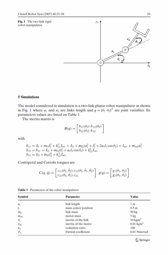
Fig. 1 The two-link rigidrobot manipulator

5 Simulations

The model considered in simulation is a two-link planar robot manipulator as shownin Fig. 1 where a1 and a2 are links length and q = [θ1 θ2]T are joint variables. Itsparameters values are listed on Table 1.

The inertia matrix is

B(q) =[

b11(θ2) b 12(θ2)

b21(θ2) b 22

]

with

b11 = Il1 + ml1l21 + k2

r1 Im1 + Il2 + ml2(a21 + l2

2 + 2a1l2 cos θ2) + Im1 + mm2a21

b12 = b21 = Il2 + ml2(l22 + a1l2 cos θ2) + k2

r2 Im1

b11 = Il2 + ml2l22 + k2

r2 Im1

Centripetal and Coriolis torques are

C(q, q) =[

c11(θ2, θ2) c12(θ2, θ1, θ2)

c21(θ2, θ1) c22

]g(q) =

[g1(θ1, θ2)

g2(θ1, θ2)

]

Table 1 Parameters of the robot manipulator

Symbol Parameter Value

ai link length 1 mli mass center position 0.5 mmll link mass 50 kgmmi motor mass 5 kgIli inertia of the link 10 kgm2

Imi inertia of the motor 0.01 kgm2

kri reduction ratio 100Fvi friction coefficient 0.01 Nms/rad


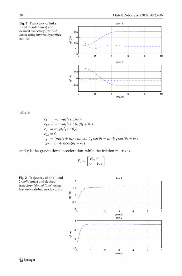
Fig. 2 Trajectory of links1 and 2 (solid lines) anddesired trajectory (dashedlines) using inverse dynamicscontrol

0 2 4 6 8 10–1.5

–1

–0.5

0

0.5

1joint 1

q2 [m

]

0 2 4 6 8 10–1

–0.5

0

0.5

1joint 2

time [s]

q2 [m

]

where

c11 = −ml2a1l2 sin θ2θ2

c12 = −ml2a1l2 sin θ2(θ1 + θ2)

c21 = ml2a1l2 sin θ2θ1

c22 = 0g1 = (ml1l1 + ml2a1mm2a1)g cos θ1 + ml2l2g cos(θ1 + θ2)

g2 = ml2l2g cos(θ1 + θ2)

and g is the gravitational acceleration, while the friction matrix is

Fv =[

Fv1 00 Fv1

]

Fig. 3 Trajectory of link 1 and2 (solid lines) and desiredtrajectory (dotted lines) usingfirst order sliding mode control

0 1 2 3 4 5 60

0.5

1

1.5

2

q1 [m

]

link 1

time [s]

0 1 2 3 4 5 6–2

0

2

4link 2

time [s]

q2 [m

]


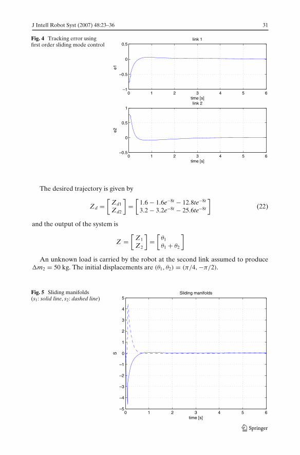
Fig. 4 Tracking error usingfirst order sliding mode control

0 1 2 3 4 5 6–1

–0.5

0

0.5

e1

link 1

time [s]

0 1 2 3 4 5 6–0.5

0

0.5

1link 2

time [s]

e2

The desired trajectory is given by

Zd =[

Zd1

Zd2

]=

[1.6 − 1.6e−8t − 12.8te−8t

3.2 − 3.2e−8t − 25.6te−8t

](22)

and the output of the system is

Z =[

Z1

Z2

]=

[θ1

θ1 + θ2

]

An unknown load is carried by the robot at the second link assumed to produce�m2 = 50 kg. The initial displacements are (θ1, θ2) = (π/4,−π/2).

Fig. 5 Sliding manifolds(s1: solid line, s2: dashed line)

0 1 2 3 4 5 6–5

–4

–3

–2

–1

0

1

2

3

4

5Sliding manifolds

time [s]

S


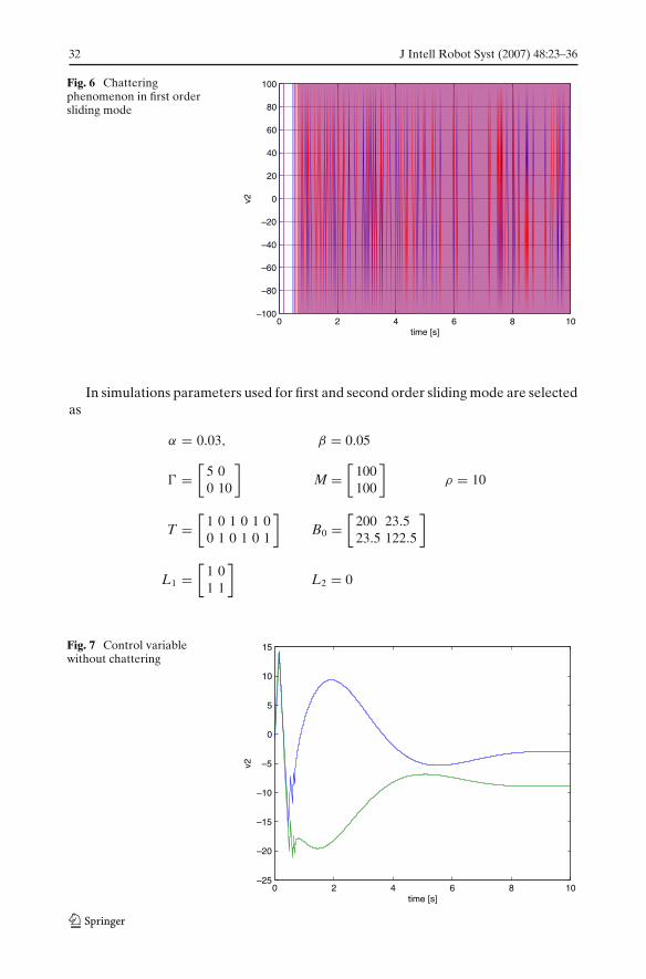
Fig. 6 Chatteringphenomenon in first ordersliding mode

0 2 4 6 8 10–100

–80

–60

–40

–20

0

20

40

60

80

100

time [s]

v2

In simulations parameters used for first and second order sliding mode are selectedas

α = 0.03, β = 0.05

� =[

5 00 10

]M =

[100100

]ρ = 10

T =[

1 0 1 0 1 00 1 0 1 0 1

]B0 =

[200 23.523.5 122.5

]

L1 =[

1 01 1

]L2 = 0

Fig. 7 Control variablewithout chattering

0 2 4 6 8 10–25

–20

–15

–10

–5

0

5

10

15

time [s]

v2


Fig. 8 Condition s = 0 is notsatisfied using the smoothapproximation

0 0.5 1 1.5 2–0.7

–0.6

–0.5

–0.4

–0.3

–0.2

–0.1

0

0.1

0.2Sliding manifolds

time [s]

S

and the control gains are selected as

Kv =[

7 00 10

]Kp =

[35 00 70

]Ki =

[20 00 45

]

Figure 2 shows that, using the inverse dynamics control when the unknown load iscarried by the robot at the second link, the performance of the system is poor, i.e. thetracking error does not converge to zero.

In Fig. 3 simulations results are reported using the first order sliding mode controllaw presented in Section 3, demonstrating that the controlled output tracks thedesired reference trajectory although the dynamics of the system is affected byuncertainties.

Fig. 9 Trajectory of link 1 and2 (solid lines) and desiredtrajectory (dotted lines) usingsecond order sliding modecontrol

0 2 4 6 8 100

0.5

1

1.5

2link 1

time [s]

q1

0 2 4 6 8 10–2

0

2

4link 2

time [s]

q2


Fig. 10 Tracking error usingsecond order sliding modecontrol

0 2 4 6 8 10–1

–0.5

0

0.5

1

time [s]

S1

0 2 4 6 8 10–2

–1.5

–1

–0.5

0

0.5

time [s]

S2

The goal of sliding mode control is to force the trajectory error e to zero so thatthe selected output tracks the desired reference trajectory (22) as shown in Fig. 4.

Convergence of the system to the sliding manifold is assured as shown in Fig. 5. InFig. 6 one can see chattering phenomena, which always appears in first order slidingmode.

To overcome this problem it is possible to replace the discontinuous termT Ax(ST T Ax)T/

∥∥ST T Ax∥∥ used in Eq. 16 with a smooth approximation given by

Vapp = T Ax(ST T Ax)T∥∥ST T Ax∥∥ + αe−βt

Fig. 11 Second order slidingmode control law

0 2 4 6 8 10–25

–20

–15

–10

–5

0

5

10

15

time [s]

v2


so that Eq. 16 becomes

ν2 = −L1 B−10 M − L2q − ρ(T B)−1T Ax(ST T Ax)T∥∥ST T Ax

∥∥ + αe−βt− (T B)−1�S (23)

reducing the chattering phenomenon as shown in Fig. 7. The major drawback ofthis approach is that the state of the system does not converge exactly to the slidingmanifold, so that condition s = 0 can not be assured, as reported on Fig. 8.

Figure 9 shows that using second order sliding mode control the controlled outputtracks the desired reference trajectory and Fig. 10 demonstrates that the trackingerror is forced to zero. Moreover, using second order sliding mode the chatteringeffect is mitigated as shown in Fig. 11.

6 Conclusions

A new motion control strategy for rigid robot manipulators is presented in thispaper using a combination of sliding mode control techniques and compensatedinverse dynamics method. The proposed control scheme does not require an on-linecalculation of the time-varying inertia matrix, providing robustness versus matcheduncertainties and disturbances. The second order sliding mode control law allowsto mitigate chattering problems by confining discontinuities to the derivative of thecontrol law. Simulations results demonstrate the good performances of the proposedcontrol strategy.

References

1. Abdallah, C., Dawson, D., Dorato, P., Jamshidi, M.: Survey of robust control of rigid robots.IEEE Control Syst. Mag. 11(2), 24–30 (1991)

2. Adam, M.J.K.: Basics of Robotics: Theory and Components of Manipulators and Robots.Springer, Berlin Heidelberg New York (1999)

3. Asada, H., Slotine, J.-J.E.: Robot Analysis and Control. Wiley, New York (1986)4. Chen, Y.-P., Chang, J.-L.: Sliding-mode force control of manipulators. Proc. Natl. Sci. Counc.,

Repub. China 23(2), 281–289 (1999)5. Bartolini, G., Ferrara, A., Usai, E.: Chattering avoidance by second order sliding mode control.

IEEE Trans. Automat. Contr. 43, 241–246 (1998)6. Bartolini, G., Ferrara, A., Usai, E., Utkin, V.I.: On multi-input chattering-free second-order

sliding mode control. IEEE Trans. Automat. Contr. 45(9), 1711–1717 (2000)7. Ibrahimbegovic, A., Knopf-Lenoir, C., Kucerova, A., Villon, P.: Optimal design and optimal

control of elastic structures undergoing finite rotations. Int. J. Numer. Methods Eng. 61(14),2428–2460 (2004)

8. Juang, J.-N., Eure, K.W.: Predictive feedback and feedforward control for systems with unknowndisturbance. NASA/Tm-1998-208744 (1998)

9. Kuo, C.Y., Wang, S.P.T.: Nonlinear robust industrial robot control. Trans. ASME, J. Dyn. Syst.Meas. Control 11, 24–30 (1989)

10. Perk, J.-S., Han, G.-S., Ahn, H.-S., Kim, D.-H.: Adaptive approaches on the sliding mode controlof robot manipulators. Trans. Control, Autom. Syst. Eng. 3(2), 15–20 (2001)

11. Shyu, K.-K., Chu, P.-H., Shang, L.-J.: Control of rigid manipulators via combiantion of adaptivesliding mode control and compensated inverse dynamics approach. IEE Proc., Control TheoryAppl. 143(3), 283–288 (1996)


12. Spong, M.W., Lewis, F.L., Abdallah, C.: Robot Control: Dynamics, Motion Planning, and Analy-sis. IEEE Press, New York (1993)

13. Edwards, C., Spurgeon, S. K.: Sliding Mode Control: Theory and Applications. Taylor & Francis,London, United Kingdom (1998)

14. Utkin, V.I.: Sliding Modes in Control Optimization. Springer, Berlin Heidelberg New York(1992)

Motion Control of Rigid Robot Manipulators via First and Second Order Sliding Modes

Documents

Transcript of Motion Control of Rigid Robot Manipulators via First and Second Order Sliding Modes