energies

Article

Fault Coverage-Aware Metrics for Evaluating the ReliabilityFactor of Solar Tracking Systems

Raul Rotar * , Sorin Liviu Jurj , Flavius Opritoiu and Mircea Vladutiu

�����������������

Citation: Rotar, R.; Jurj, S.L.;

Opritoiu, F.; Vladutiu, M. Fault

Coverage-Aware Metrics for

Evaluating the Reliability Factor of

Solar Tracking Systems. Energies 2021,

14, 1074. https://doi.org/10.3390/

en14041074

Received: 8 December 2020

Accepted: 16 February 2021

Published: 18 February 2021

Publisher’s Note: MDPI stays neutral

with regard to jurisdictional claims in

published maps and institutional affil-

iations.

Copyright: © 2021 by the authors.

Licensee MDPI, Basel, Switzerland.

This article is an open access article

distributed under the terms and

conditions of the Creative Commons

Attribution (CC BY) license (https://

creativecommons.org/licenses/by/

4.0/).

Computers and Information Technology, “Politehnica” University of Timisoara, 2 V. Parvan Blvd,300223 Timisoara, Romania; jurjsorinliviu@yahoo.de (S.L.J.); flavius.opritoiu@cs.upt.ro (F.O.);mircea.vladutiu@cs.upt.ro (M.V.)* Correspondence: raul.rotar@student.upt.ro

Abstract: This paper presents a mathematical approach for determining the reliability of solartracking systems based on three fault coverage-aware metrics which use system error data fromhardware, software as well as in-circuit testing (ICT) techniques, to calculate a solar test factor (STF).Using Euler’s named constant, the solar reliability factor (SRF) is computed to define the robustnessand availability of modern, high-performance solar tracking systems. The experimental cases whichwere run in the Mathcad software suite and the Python programming environment show that thefault coverage-aware metrics greatly change the test and reliability factor curve of solar trackingsystems, achieving significantly reduced calculation steps and computation time.

Keywords: solar tracking systems; solar test factor; solar reliability factor; availability; fault coverage

1. Introduction

The most abundant form of energy on our planet is incontestably the Sun. Despitedropping technology costs and free sunlight, conventional companies have been reluctantto use photovoltaic (PV) panels such as those installed on residences’ rooftops for large-scaleprojects. Concerning this aspect, the main explanation is given by the fact that researchershave developed metrics for producing electricity from coal, gas, oil, and nuclear energy,but not from PV panels, a rapidly emerging technology whose cost depends on the Sun’savailability. Fortunately, the solar industry has started to follow a standardized metric thatconsumers can understand, generally referred to as the levelized cost of energy (LCOE) [1].In simple terms, LCOE is measured in cents per Kilowatt-hour (kWh), takes into accountall the costs of a solar plant over its lifespan, compares them to the total electrical output,and offers an accurate, long-term financial overview. This metric is commonly recognizedby the power industry, service companies, and government agencies worldwide. The solarindustry has traditionally used an alternative metric, called dollars per watt [2] whichcompares the initial costs of a solar installation against its potential peak power output.This metric, if taken on its own, lacks the actual energy generated by the solar system andmany other variables which are the strong points of the LCOE metrics.

The multitude of LCOE variables [3] can be grouped into five main categories: (a)location (for Sun exposure, seasonality, and local benefits); (b) cost of capital (spanninginterest, taxes, and leverage); (c) energy production (solar panel and automated equipmentperformance evaluation); (d) system costs (similar to dollars per Watt, but covers the totalinstallation costs as well as warranties); (e) operations and maintenance costs (cleaning,monitoring and repairing). Since it is out of scope for this paper to cover all possiblecategories offered by the LCOE metrics suite, our field of research is restricted to theenergy production and maintenance costs domains. Conceptually, regarding the energyproduction domain, more daylight, more powerful PV panels and more reliable Sunavailability translates into more electricity. However, a few aspects are counter-productive,as cold days are better than hot days for solar production, since PV cells overheating

Energies 2021, 14, 1074. https://doi.org/10.3390/en14041074 https://www.mdpi.com/journal/energies

Energies 2021, 14, 1074 2 of 24

can lower energy output [4]. To compensate for the environmental weather conditions,solar tracking systems are used nowadays to steer PV panels according to the Sun’sdirection, thereby increasing energy production which will significantly boost the returnon investment. Regarding operations and maintenance costs, one of the key elements forlong-term performance from a solar tracking device is the requirement of high reliability,remote monitoring, proactive maintenance, and service [5]. Thus, proper selection ofelectrical equipment is crucial for constructing a robust and long-lasting solar trackingsystem that will maximize solar energy collection. Since solar trackers can be assembledfrom individual circuits such as microcontroller units (MCUs, Arduino, SMT32 boards),motor drivers (L298N, ULN2003A), DC-DC and stepper motors, it is vital to emphasizethat each of these electrical components can become faulty during their operation. Hence,several testing methods were developed to detect software [6], hardware [7] as well asin-circuit [8] errors in dual-axis solar tracking equipment, and to ultimately counteract thenegative effects of a malfunctioning or, in more critical scenarios, system failure.

Since LCOE calculation formulas are overly complex for computing the reliabilityof solar tracking systems, this paper proposes a set of three fault-coverage aware metricsthat calculate an STF based on the number of detected errors and determines the SRFthat categorizes and certifies the quality of modern, and high-performance dual-axis solartracking systems.

The paper is organized as follows: Section 2 presents several works related to recentmetrics developed to assess the efficiency and reliability of solar panels. Section 3 describesthe most common metrics for evaluating the meantime to failure as well as the reliabilityof automated solar systems according to the well-known Weibull distribution model.Section 4 introduces the proposed metrics for calculating the STF as well as the SRF of solartracking systems. Section 5 presents the experimental setup and results. Finally, Section 6concludes this paper.

2. Literature Review

Even though LCOE metrics became today’s standard for choosing reliable and effi-cient solar tracking systems [9,10], the author in [11] demonstrates that LCOE inaccuratelydisfavors renewable energy sources. Furthermore, based on his research, the LCOE equa-tion which was formulated by the U.S. National Renewable Energy Laboratory (NERL)overprices solar energy by 27%, and wind energy by 18% as compared to natural gas-basedpower, showing that the LCOE model will be potentially replaced in the future by newmetrics called “present value of the cost of energy” (PVCOE).

Recent advancements in the field of renewable energy show that besides the standardLCOE metrics formulas, other solar-energy oriented metrics have been developed forassessing the performance and reliability of static solar PV systems. Along with the solartracking methods which are used to optimize the PV panel’s position towards the Sun, newtechniques such as solar power forecasting were introduced to the market to improve theperformance and reliability of solar PV panels. Thus, the authors in [12] present a collectionof value-based solar forecasting metrics that can be applied to a variety of input variables(various time horizons, geographic locations, and applications) to improve the accuracyof solar forecasting capabilities. Additionally, the authors implement a framework for asystematic approach to evaluate the sensitivity of the proposed metrics to three types ofsolar forecasting improvements (uniform improvements, ramp forecasting magnitude im-provements, and ramp forecasting threshold adjustment). Their experimental results showthat the proposed metrics offer an efficient evaluation of solar power forecasts and high-light the economic and reliability effects of improved solar energy forecasts. Researchersfrom the U.S. NREL associate the term reliability with stability in their work [13], whichinvolves a study of transient stability, frequency response, control stability, and the impactof concentrating solar power (CSP) on grid reliability. Their investigation demonstratesthat large amounts of CSP units do not pose any challenge to grid stability, and that fre-quency response can be enhanced significantly by frequency sensitive controls on CSP

Energies 2021, 14, 1074 3 of 24

and solar PV installations. Furthermore, another team of research scientists from the sameinstitute highlights the role of reliability and durability in PV system economics [14]. Byimproving the conventional LCOE metrics formula with the system architecture cost, acapacity factor (system location, orientation, tracking), and a reliability and durabilityexpression, they were able to determine the total life cycle cost divided by the total lifetimeenergy production.

On the other hand, the authors in [15] propose an optimal modeling and metricsdesign for solar energy-powered base stations, proving that 4G cellular communicationunits can benefit from complete clean energy in the future. The authors establish a model fordescribing the dynamic behavior of solar energy-based base stations by using a stochasticqueue model, and further develop three performance metrics (service outage probability,solar energy utilization efficiency, and mean depth of discharge) which will form the keyelement for their minimization algorithm that takes into consideration the communicationreliability, efficiency, and durability. The United Nations Sustainable Development Goalsno. 7 indicates a major global task: “Ensure access to affordable, reliable, sustainable,and modern energy for all” [16]. The authors in [17] adhere to this goal and address theproblem of reliability cost in decentralized solar power systems in sub-Saharan regions. Byemploying a multi-step optimization algorithm based on the LCOE metrics, the authorsachieve a 90% reduction of energy cost for household solar systems with battery storagein Africa.

Recent efforts in the field of green energy have been also made to introduce the term“availability” to the standards, contract language, and performance models of PV systems.Therefore, the authors in [18] define availability as the operational status of an electricalenergy generating technology, which gives a hint about the component health and systemreliability (uptime, downtime, and condition stages). Moreover, availability is described asthe fraction of time in which an industrial unit is capable of providing service to generateenergy, so that reliability in this scenario is purely given by a probabilistic model, whichwill be extended later in this paper. Following, the authors in [19] present a comprehensivestudy of a large PV system involving field data, failure times, and repair times for fiveyears. Their reliability program, which strengthens the interaction between reliabilitymodel, failure model, and accelerated tests, shows that periodic maintenance and repairoperations are vital for system availability since the granularity of the proposed modelis given by the level of collected failure data. These scientific findings direct us to a newapproach in the reliability domain where the predicted number of component failuresbecomes extremely important, thus opening the path to developing new metrics based onfault coverage.

This paper distinguishes itself from the above-mentioned works by proposing threemetrics that take into consideration the fault coverage obtained from the testing methodsthat were applied to modern dual-axis solar tracking systems. More precisely, an STF iscomputed that considers software, hardware, and in-circuit errors, thus determining theSRF that defines the quality, reliability, robustness, and durability of mobile solar trackers.

3. The Weibull Distribution Model for Calculating the Reliability of Dual-Axis SolarTracking Systems

During the construction of various automation equipment, the requirement to ensuretheir safe operation has led to the use of certain safety factors in their design. The notionsof reliability and safety in operation have emerged and highlighted the concern for find-ing mathematical models and calculation methods that allow making the most accuratepredictions regarding the behavior, over a certain period, of installations and equipmentin conditions of known exploitation. Reliability, from the maintenance point of view, is aprobability representing the ability of a product to function without defects, involving aslight chance of failure, and can be expressed mathematically as in Equation (1) [20]:

R(t) + F(t) = 1 (1)

Energies 2021, 14, 1074 4 of 24

where R is the probability that the product will continue to meet the specifications, and Fdenotes the probability of failure, both variables being time functions, depending on theparameter t. The advantage of relation (1) is that it can be applied to systems that are fullyfunctional or fully defective. In our context, if a chain of solar tracking systems containsirreparable products (most unfavorable scenario), the corresponding reliability curve willlook like the one presented in Figure 1.

Figure 1. Reliability (R) and Final Moment (T) to Failure for N solar tracking systems [20].

As can be seen in Figure 1, the computation of the reliability factor denoted with Rrelies on N products (solar tracking systems) and the final moment, denoted with T, inwhich all the components of the products are completely damaged.

3.1. Failure Frequency (Hazard Rate)

The failure frequency, also known as hazard rate, describes how many products areout of service (malfunctioning) in a given period. The mathematical expression associatedwith the failure frequency is given by Equation (2) [20]:

λ =N

N∑

i=1Ti

=1

MTF(2)

where λ denotes the failure frequency, N the total number of products, Ti the correspondingtime failures for each of the N products (industrial components), and the Mean Time toFailure (MTF) represents the average time to failure. The reliability equation will be writtenas in (3) [20]:

Ri =N − i

N(3)

where N–i designates the number of surviving products and N the total number of products.The reliability curve diagram can be drawn accordingly as presented in Figure 2.

Figure 2. Reliability Curve Linear Function at moment 0 and moment T for a chain of solar trackingsystems [20].

The derived linear reliability function can be expressed as in (4) [20]:

R(t) = at + b (4)

Energies 2021, 14, 1074 5 of 24

where a denotes a random coordinate of the X-axis, and b denotes a random value fromthe Y-axis. First, according to Figure 2, the reliability linear function will be computed atmoment t = 0, to determine the coordinate b, as presented in Equation (4a):

R(t) = at + b = 1R(0) = 0t + b = 1→ b = 1

(4a)

Secondly, since we know that at t = T (final moment) the reliability will be 0, coordinatea can be computed as presented in relation (4b):

R(T) = aT + b = 0R(T) = aT + 1 = 0→ a = − 1

T(4b)

According to relations (4a) and (4b), the reliability linear function can be rewritten asin Equation (5):

R = − tT+ 1 (5)

Consider, for a more concrete case, that a test was performed on a chain of 15 PVsensors (in our case, PV cells) that are used to automate solar tracking equipment. The testtime is measured in units of days. The measurement times were collected and orderedin Table 1.

Table 1. Collected failure times for each of the N products.

Failure Moments (Ti) Ti (Days)

T1 125T2 170.83T3 220.83T4 283.3T5 291.6T6 341.6T7 375T8 512.5T9 541.6T10 583.3T11 625T12 666.6T13 687.5T14 741.6T15 795.83

First, for all the collected failure times, the associated MTF and hazard rate can bedetermined for the solar tracker’s sensor modules. According to Equation (2), the MTFformula can be rewritten as in (6) [20]:

MTF =1N

N

∑i=1

Ti (6)

In other words, the MTF is given by the total test time divided by the total number offailures during testing phases. The MTF expression is calculated according to the catalogdata from Table 1, as in expression (6a):

MTF =1N

N

∑i=1

Ti =115

(125 + 170.83 + 220.83 + 283.3 + . . . + 795.83) =

=115· 6962.09 =

6962.0915

= 464.1393 days (6a)

Energies 2021, 14, 1074 6 of 24

The corresponding failure frequency will be determined from relation (2) as seen inexpression (6b):

λ =1

MTF=

1464.1393

= 0.0021545 days−1 (6b)

To establish the relative error (E) of our previous calculus, the MTF will be calculateda second time by using the following linear interpolation function of the reliability thatdepends on the time parameter as presented in relation (7) [20]:

∞∫0

R(t)dt (7)

Thus, the new MTF formula will be written as in Formula (8):

MTF1 =1λ=

10.0021545

= 464.1393 days (8)

By subtracting the MTF1 from the initial MTF relation and by dividing the result bythe average time to failure, the expression (9) will be obtained as follows:

E =MTF1 −MTF

MTF=

464.1393− 464.1393464.1393

=0

464.1393= 0% (9)

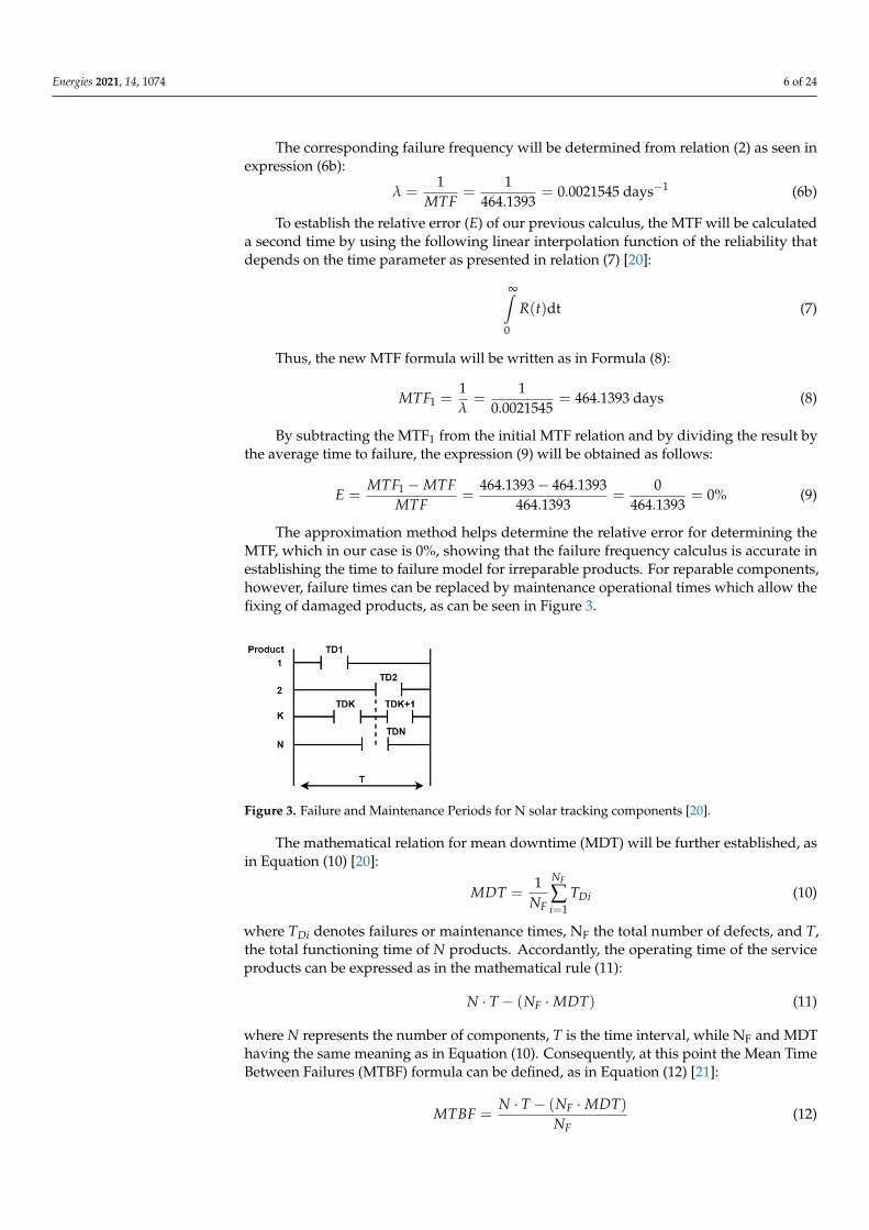
The approximation method helps determine the relative error for determining theMTF, which in our case is 0%, showing that the failure frequency calculus is accurate inestablishing the time to failure model for irreparable products. For reparable components,however, failure times can be replaced by maintenance operational times which allow thefixing of damaged products, as can be seen in Figure 3.

Figure 3. Failure and Maintenance Periods for N solar tracking components [20].

The mathematical relation for mean downtime (MDT) will be further established, asin Equation (10) [20]:

MDT =1

NF

NF

∑i=1

TDi (10)

where TDi denotes failures or maintenance times, NF the total number of defects, and T,the total functioning time of N products. Accordantly, the operating time of the serviceproducts can be expressed as in the mathematical rule (11):

N · T − (NF ·MDT) (11)

where N represents the number of components, T is the time interval, while NF and MDThaving the same meaning as in Equation (10). Consequently, at this point the Mean TimeBetween Failures (MTBF) formula can be defined, as in Equation (12) [21]:

MTBF =N · T − (NF ·MDT)

NF(12)

Energies 2021, 14, 1074 7 of 24

where the MTBF is the total operating time of all components divided by the number ofoccurring defects. The associated failure frequency (hazard rate) can be thus calculatedwith the relation (13):

1MTBF

=NF

N · T − (NF ·MDT)(13)

3.2. Availability (Efficiency)

Availability is defined as the ability of a system/equipment to be in working orderunder given conditions, at a given time, or for a given period, assuming that the provisionof the necessary external means (maintenance) is ensured [13]. Availability is consid-ered a complex form of assessing the quality of a system/product because it includesboth reliability and maintainability. Mathematically, availability can be expressed as inEquation (14) [20]:

A =N · T − NF ·MDT

N · T (14)

Based on Equation (12) the formula for the product N·T can be rewritten as in rela-tion (15):

N · T = NF ·MTBF + NF ·MDT (15)

According to Equation (15) we can now write the final form of A from (14):

A =MTBF

MTBF + MDT(16)

where, for convenience, the MTF and MTBF parameters can be used to characterize theautomated system. In conclusion, a product or component is available as long as it canprovide service, and unavailable when it is undergoing maintenance operations. As seenin Equation (1), the probability model of availability and unavailability can be expressed asin the mathematical rule (17) [20]:

A + U = 1→ U = 1− A (17)

More generally, we will write unavailability as in the Equation (18):

U =MDT

MTBF + MDT(18)

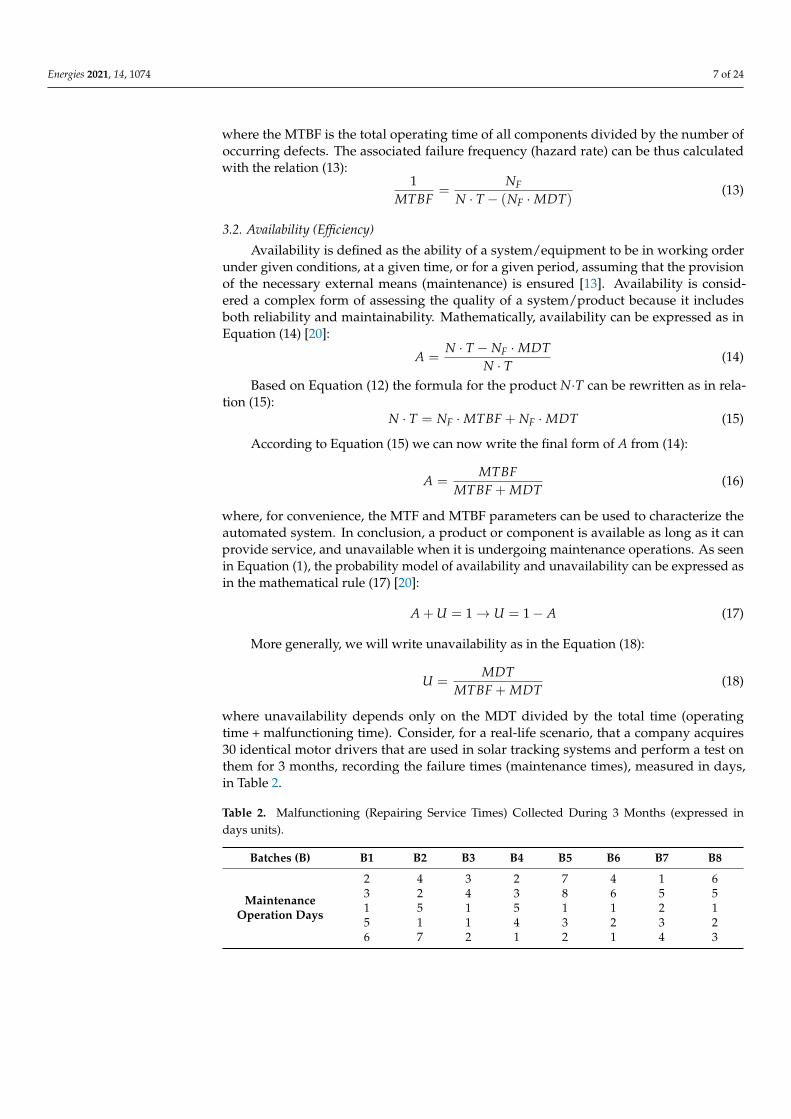
where unavailability depends only on the MDT divided by the total time (operatingtime + malfunctioning time). Consider, for a real-life scenario, that a company acquires30 identical motor drivers that are used in solar tracking systems and perform a test onthem for 3 months, recording the failure times (maintenance times), measured in days,in Table 2.

Table 2. Malfunctioning (Repairing Service Times) Collected During 3 Months (expressed indays units).

Batches (B) B1 B2 B3 B4 B5 B6 B7 B8

MaintenanceOperation Days

2 4 3 2 7 4 1 63 2 4 3 8 6 5 51 5 1 5 1 1 2 15 1 1 4 3 2 3 26 7 2 1 2 1 4 3

Energies 2021, 14, 1074 8 of 24

According to Table 2, the active number of failures is NF = 40. The total time iscalculated for NT = 30 ·90 ·24 = 64800 h = 2700 days. Accordingly, we can compute theMDT parameter with the relation (19):

MDT = 1NF

NF∑

i=1TDi =

140 (2 + 3 + 1 + 5 + 6 + . . . + 3) =

= 140 · 129 = 3.225 days

(19)

The total failure time will then be calculated with the Formula (20):

NF ·MDT = 40 · 3.225 = 129 days (20)

Furthermore, the MTBF will be determined with relation (21):

MTBF = N·T−(NF ·MDT)NF

= 30·90−129129 =

= 2700−129129 = 2571

129 = 19.93 days(21)

The failure frequency will be computed with Equation (22):

λ = 1MTBF = NF

N·T−(NF ·MDT) =129

30·90−129 =

1292700−129 = 129

2671 = 0.05(22)

At this point the availability and unavailability parameters (Equations (16), (17), and(18)) can be established based on the previously calculated values with Formula (23):

A = MTBFMTBF+MDT = 19.9

19.9+3.225 = 19.923.125 = 0.86

U = MDTMTBF+MDT = 3.225

19.9+3.225 = 3.25520.925 = 0.14

A + U = 0.86 + 0.14 = 1

(23)

By relying on the previous standard metrics, the general conclusion is that the MTBFis 19.9 days and the MTF is 3.225 days, which means that once every approximately19 days one motor driver malfunctions and requires 3.225 days for maintenance operations,resulting in an 86% availability rating and 14% unavailability rating.

3.3. Typical Variation Form of the Hazard Rate (Bathtub Curve)

The variation in time of the reliability function (R) in regards to the hazard rate (λ)can be expressed mathematically as in Equation (24) [21]:

dRR

= −λ(t)dt (24)

It was already stated that at moment t = 0 all the products function according to theiroperating specifications so that the relationship between reliability and the instantaneousfailure rate is established with the help of the equation system (25) [21]: R(t) = e

−t∫

0λ(t)dt

λ = ct→ R(t) = e

−λt∫

0dt= e−λt (25)

Generally, the MTF relation will become as presented in (26):{∆F(t) = R(t) + F(t)

F(t) = 1− e−λt → MTF =1λ

(26)

Energies 2021, 14, 1074 9 of 24

The MTF Formula (27) is given consequently by the subgraph area:

MTF =

∞∫0

R(t)dt =1λ

(27)

The graphical representation of Equation (26) can be seen in Figure 4.

Figure 4. Bathtub Curve representation of Run-In period (I), Operating Period (II), and CatastrophicFailure Period (III) [21].

This graphical representation applies to any solar tracking system (automation equip-ment) which is described by the run-in period (usually around 6 months) followed by thenormal operating period (warranty period, which depends on the quality of the acquiredproduct) and, lastly, the catastrophic defect area where generally, a solar tracking systemwill require several maintenance human interventions.

Finally, there is a second and last approach for analyzing the typical variation formof the hazard rate, given by the so-called Weibull distribution model, found in rela-tion (28) [21]:

λ(t) =β

η(

t− t0

η)

β−1, β > 0 (28)

According to Equation (28), the relation for the reliability variation can be written inthe Equation (29):

R(t) = exp[−( t− t0

η)

β](29)

where β is a positional parameter, η is a scalar parameter, t0 is the initial moment, and exprepresents the exponential form of Euler’s constant named value.

3.4. Applications

The abovementioned metrics can be applied to a variety of real-life scenarios regardingthe calculus of reliability, MTF, MDT, and hazard rate of solar tracking systems. Morespecifically, to establish accurate predictions about the reliability of the entire solar trackingsystem, it is of major importance to formulate problems concerning the failure rates ofa solar tracker’s components. For instance, consider that an MCU (e.g., Arduino UNO)which is used to control solar tracking equipment, has a constant failure rate of 0.1 / year,

Energies 2021, 14, 1074 10 of 24

and we want to determine the reliability, respectively the probability of failure for 1, 2, and3 years. This problem can be solved by just relying on the equation set (30) as follows:

R(t) = e−

t∫0

λ(t)dt

R(t) = e−λt

R(1 year) = e−0.1×1 = e−0.1 = 0.9048 = 90.48%

F(1 year) = 1− R(year) = 0.0952 = 9.52%

R(2 years) = e−0.1×2 = e−0.2 = 0.8187 = 81.87%

F(2 years) = 1− R(2 years) = 0.1813 = 18.13%

R(3 years) = e−0.1×3 = e−0.3 = 0.7408 = 74.08%

F(3 years) = 1− R(3 years) = 0.2592 = 25.92%

(30)

The aforementioned solution shows that the reliability of the Arduino UNO boarddecreases in years by an average value of 8%, while the chance of failure increases everyyear by approximately 9%. Another way to analyze the behavior of solar tracking systems isfrom the defects points of view, according to a Weibull distribution given by the parameterst0 = 0, η = 625 days and β = 1.5. It is considered that for the given input parameters, atest was performed on 1000 random components that were mass-produced to constructsolar trackers. The goal here is to determine the survival (operating) probability of thesecomponents after t = 104 h, by applying the Weibull equation, as presented in (31):

R(t) = exp[−( t−t0

η )β]= exp

[−( 416.6−0

625 )1.5]= exp

[−( 416.6

625 )1.5]=

= exp(−0.5442) = 0.5803 = 58.03%(31)

Additionally, for another queue of 1000 random components that were mass-producedin the industrial environment, it is of interest to determine the period after which 100 com-ponents became faulty. It is assumed that the component testing was started at the momentt = 0. Therefore, if t0 = 1000 components, moment t1 will correspond to the subtractionof 100 components from the initial stack, in other words, t1 = 1000 – 100 = 900 remainingcomponents. The associated reliability R(t0) = 1 (as a general rule) and R(t1) = 0.9. Theexpression of R(t1) is expanded according to Formula (32):

R(t1) = exp[−( t1−t0

η )β]

ln R(t1) = ln[exp

[−( t1−t0

η )β]]→ ln R(t1) = −( t1−t0

η )β

ln 1R(t1)

= ( t1−t0η )

β → ln ln 1R(t1)

= β · ln(t1 − t0)− β · ln η

→ ln(t1 − t0) = (ln ln 1R(t1)

+ β · ln η) · 1β

(32)

Following, the last obtained expression for t0 = 0 will be computed as in (33):

t1 = e1β (ln ln 1

R(t1)+β ln η) → t1 = e

11.5 (ln ln 1

0.9+1.5 ln 1.5·104) →

→ t1 = e1

1.5 (−2.25+9.6158) → t1 = 0.38170987 years(33)

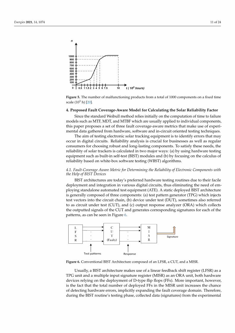
Finally, a more convenient manner to represent the number of faulty components isthrough a graph chart which shows the evolution in time of 10 pairs containing 100 compo-nents each, until the final moment where all products are completely damaged, as can beseen in Figure 5.

Energies 2021, 14, 1074 11 of 24

Figure 5. The number of malfunctioning products from a total of 1000 components on a fixed timescale (103 h) [20].

4. Proposed Fault Coverage-Aware Model for Calculating the Solar Reliability Factor

Since the standard Weibull method relies initially on the computation of time to failuremodels such as MTF, MDT, and MTBF which are usually applied to individual components,this paper proposes a set of three fault coverage-aware metrics that make use of experi-mental data gathered from hardware, software and in-circuit oriented testing techniques.

The aim of testing electronic solar tracking equipment is to identify errors that mayoccur in digital circuits. Reliability analysis is crucial for businesses as well as regularconsumers for choosing robust and long-lasting components. To satisfy these needs, thereliability of solar trackers is calculated in two major ways: (a) by using hardware testingequipment such as built-in self-test (BIST) modules and (b) by focusing on the calculus ofreliability based on white-box software testing (WBST) algorithms.

4.1. Fault-Coverage Aware Metric for Determining the Reliability of Electronic Components withthe Help of BIST Devices

BIST architectures are today’s preferred hardware testing routines due to their faciledeployment and integration in various digital circuits, thus eliminating the need of em-ploying standalone automated test equipment (ATE). A static deployed BIST architectureis generally composed of three components: (a) test pattern generator (TPG) which injectstest vectors into the circuit chain, (b) device under test (DUT), sometimes also referredto as circuit under test (CUT), and (c) output response analyzer (ORA) which collectsthe outputted signals of the CUT and generates corresponding signatures for each of thepatterns, as can be seen in Figure 6.

Figure 6. Conventional BIST Architecture composed of an LFSR, a CUT, and a MISR.

Usually, a BIST architecture makes use of a linear feedback shift register (LFSR) as aTPG unit and a multiple input signature register (MISR) as an ORA unit, both hardwaredevices relying on the deployment of D-type flip flops (FFs). More important, however,is the fact that the total number of deployed FFs in the MISR unit increases the chanceof detecting hardware errors, implicitly expanding the fault coverage domain. Therefore,during the BIST routine’s testing phase, collected data (signatures) from the experimental

Energies 2021, 14, 1074 12 of 24

cases is used to outline the fault coverage. Further, an STF parameter is defined, which willbe expressed mathematically as in Formula (34):

STF =NE · TV

TP · 2D (34)

where TV represents the number of executed test vectors, NE the number of errors pertest case, TP the total number of test patterns, and D the number of identical devices usedfor detecting errors (which in our case are given by the FF units). Since the generalizedSTF formula can be adapted to various test scenarios, several STF properties will be listedas follows:

(1) The number of errors NE is always equal, lower, or greater than TV in any testscenario regardless of the noise factors that are considered, and can be expressedmathematically as in (35):

NE ≥ TV__NE ≤ TV__NE, TV ∈ N (35)

(2) The number of test vectors TV is always equal to or lower than the total number oftest patterns TP given by the expression (36):

TV ≤ TP__TV , TP ∈ N (36)

(3) The total number of test patterns is calculated with the Equation (37):

TP = 2D − 1 (37)

(4) If no errors are detected during the testing routines, the STF parameter will be0 resulting in 100% reliability and availability of the tested equipment, expressed inEquation (38):

STF = 0↔ R = A = 1 (38)

To demonstrate the validity of these properties, a few concrete cases are presentedfurther. Regarding the STF, the following considerations are listed: (a) for a total numberof TV = 7 (test cases) the test system has successfully identified NE = 10 bit-flip errors.It should be noted, according to property (1) that the number of errors detected may begreater than the number of test cases because multiple errors (burst errors) may occurwithin a single test vector. Additionally, for (b) a number D = 4 FFs are used in the structureof the MISR in this paper. According to property (3), the total number of test cases TP iscalculated based on the Formula (39):

TP = 2D − 1→ TP = 24 − 1 = 15 (39)

Since TV = 7 and TP = 10 property (2) is also satisfied. Finally, by having this hypothet-ical data the variables from Equation (34) can be adequately substituted as in (40):

STF =10 · 7

15 · 16=

70240

= 0.29 ≈ 0.30 (40)

Supposing that during the detection stage, all the errors were corrected by using theHamming code algorithms, parameter NE will be reduced to the value 0. The correspondingequation will be expressed as in (41):

STF =0 · 7

15 · 16=

0240

= 0→ R = A = 1 (41)

Energies 2021, 14, 1074 13 of 24

thus satisfying property (4) of the first set of metrics. In the last stage the SRF will becalculated with the Formula (42):

SRF = exp[NE · TV

TP · 2D ] (42)

Since the SRF expression is the exponential of the STF equation, the entire relationshipcan be rewritten as in expression (43):

SRF = e−STF (43)

At this point, the SRF of the automated sun-tracking equipment will be computed asin Equation (44):

SRF = e−STF = e−0.3 =1

e0.3 =1

2.710,3 =1

1.3486= 0.74 (44)

Similarly, if the STF parameter is reduced to 0, the mathematical expression willbecome as in expression (45):

SRF = e−STF = e−0 =1e0 =

11= 1↔ R = A = 1 (45)

The final mathematical relation connects the SRF parameter with the initially com-puted STF variable according to property (4), thus showing that hardware componentsthat are not affected by permanent errors can achieve 100% reliability and availability. Anyother types of defects caused by transient errors can be considered negligible since theirfootprint on the electronic components is only temporary and does not cause any seriousharm to the overall functionality of the tested devices [6].

4.2. Fault-Coverage Aware Metric for Determining the Reliability of Electronic Components withthe Help of WBST Methods

Traditional testing processes aim to generate test vector sets that apply to a specificfault model to optimize coverage while reducing the execution time of the test application.Because the Off-Line test is typically performed after the circuit is assembled as part of amore in-depth manufacturing test, it is often used in maintenance checking for extendingthe lifespan of the product. Roughly equivalent to off-line testing, on-line testing, alsoreferred to as parallel or concurrent error detection, is a test technique used to permanentlyverify the integrity of the CUT, as can be seen in Figure 7. One of the preferred on-line software testing techniques is known under the acronym of WBST routines whichperiodically checks the CUT for transient or permanent errors. A more particular case ofthe WBST method is the cloud-based software testing technique which makes use of anInternet of Things (IoT) software TPG for injecting test vectors in MCU devices which arepart of solar tracking equipment.

Figure 7. Conventional on-line testing mechanism composed of a software TPG (STPG), an applica-tion under test (AUT), and an ORA.

By stimulating the inputs of the CUT the outputs are collected in a results gathererwhere with the help of an error indicator, the user is capable to establish the fault coverageof the employed WBST method. Moreover, as expected, the previous metric set presented

Energies 2021, 14, 1074 14 of 24

in Section 4.1 for our software test scenarios can be adapted adequately. The STF formulacorresponding to the WBST routines will be written as in Equation (46):

STF =NE · TV

TP · 2B (46)

where NE represents the number of errors per test vector, TV denotes the number ofconsidered test vectors, TP provides the total number of test patterns and B designatesthe number of breakpoints/software functions that are implemented across the algorithmdebugging stage.

Besides this minor difference from the proposed hardware metric, a few other proper-ties which are important for demonstrating the validity of the software-based metric willbe listed below:

(1) The number of errors NE is always equal, lower, or greater than TV in any testscenario regardless of the number of considered breakpoints, and can be expressedmathematically as in statement (47):

NE ≥ TV__NE ≤ TV__NE, TV ∈ N (47)

(2) The number of test vectors TV is always equal to or lower than the total number oftest patterns TP given by the expression (48):

TV ≤ TP__TV , TP ∈ N (48)

(3) If no errors are detected during the testing routines the STF parameter will be 0resulting in 100% reliability and availability of the tested equipment, expressed as inEquation (49):

STF = 0↔ R = A = 1 (49)

As already anticipated, the second metric removes one of the listed properties fromSection 4.1 since there is no clear mathematical relationship between the total numberof test patterns TP and the number of breakpoints B. At this point, the validity of theremaining three properties can be demonstrated in a real-life scenario. Regarding the STF,the following considerations are made: (a) for a total number TV = 7 (test cases), the testsystem has successfully identified NE = 10 calculation errors. Additionally, for (b) a numberof TP = 10 test patterns and a number B = 10 breakpoints in the software code, meaningthat the test system successfully identified all calculation errors with the deployed softwarefunctions. Because properties (1) and (2) are already satisfied from the above statement, letthe STF parameter will be calculated as in relation (50):

STF =10 · 710 · 10

=70

100= 0.70 (50)

In the last stage, the SRF parameter will be computed with the mathematical rule (51):

SRF = exp[NE ·TVTP ·2D ] = e−STF = e−0.7 = 1

e0.7 = 12.710.7 =

= 12 = 0.50

(51)

showing that with almost the same hypothetical set of data from Section 4.1, the reliabilityof the solar tracking equipment is halved. This is because calculation errors in the softwarecode usually manifest in the behavioral model of the hardware device (incoherent steppermotor rotations leading to improper positioning of the solar panel thus resulting in heavyenergy harvesting losses). Along with the satisfying property (3) of the second set ofmetrics, consider that during the detection stage all the errors were manually corrected

Energies 2021, 14, 1074 15 of 24

by the software engineer, thus minimizing NE to the value 0. The final Equation (52)will become:

SRF = e−STF = e−0 =1e0 =

11= 1↔ R = A = 1 (52)

4.3. Fault-Coverage Aware Metric for Determining the Reliability of Electronic Components withthe Help of ICT Methods

ICT is a type of white-box testing procedure where an electrical probe navigates theentire printed circuit board (PCB) area to identify shorts, opens, resistance, capacitance,and other basic electrical components which give a hint of the electronic assembly whichwas fabricated according to its catalog specifications [19]. The ICT process is conductedwith the help of industrial machines such as ATE, bed of nails fixtures, or with a fixturelessICT setup (one example here being a flying probe device). In works [19,20], a flying probeinspired in-circuit tester (FPICT) was constructed and deployed to verify the integrityof the entire solar tracking electrical equipment. By implementing a sensorless solutionfor locating all test points of the PCB, the proposed test device was capable to monitorcritical paths and parameters (such as current and voltage drops), thus determining a faultcoverage of the malfunctioning CUTs, as can be seen in Figure 8.

Figure 8. Conventional ICT block diagram composed of an FPICT, a DUT, and a Digital Monitor.

To demonstrate the flexibility of the metrics set, the mathematical expressions fromSections 4.1 and 4.2 will be adapted to the ICT test scenarios. The STF formula correspond-ing to the ICT routines will be written as in expression (53):

STF =NE · TR

NR · 2P (53)

where NE represents the number of errors per test round, TR denotes the number ofconsidered test rounds, NR provides the total number of test routines and P designates thenumber of probes (nails) that are equipped to the FPICT device.

Similarly, as in the previous sections, the properties which are essential for validatingthe ICT-based metric will be listed below:

(1) The number of errors NE is always equal, lower, or greater than TR in any test scenarioregardless of the number of probes that are used during testing, and can be expressedmathematically as in expression (54):

NE ≥ TR__NE ≤ TR__NE, TR ∈ N (54)

(2) The number of test rounds TR is always equal to or lower than the total number oftest routines NR, given by the expression (55):

TR ≤ NR__TR, NR ∈ N (55)

(3) If no errors are detected during the testing routines the STF parameter will be 0resulting in 100% reliability and availability of the tested equipment, expressed as inrelation (56):

STF = 0↔ R = A = 1 (56)

Consider a real-life scenario where all possible test points’ voltage deviations must beidentified. For this purpose, the test system implements a number of TR= 10 rounds foreach test point, a total number of NR = 100 test routines, and a number of P = 2 probes, to

Energies 2021, 14, 1074 16 of 24

identify NE = 12 voltage deviations. The STF parameter will be computed in relation (57),based on the previous configuration:

STF =NE · TR

NR · 2P =12 · 10100 · 22 =

120400

= 0.30 (57)

With the abovementioned result properties (1) and (2) are successfully satisfied. Todemonstrate property (3), a similar but fault-free DUT is considered, leading to the For-mula (58):

STF =NE · TR

NR · 2P =0 · 10

100 · 22 =0

400= 0↔ R = A = 1 (58)

The SRF parameter will be calculated as in Equations (59) and (60):

SRF = e−STF = e−0.3 =1

e0.3 =1

2.710.3 =1

1.3486= 0.74 (59)

SRF = e−STF = e−0 =1e0 =

11= 1↔ R = A = 1 (60)

The above described metrics reduce significantly the number of computations exe-cuted during the Weibull distribution algorithm, as well as the number of parameters thatare involved in the mathematical rules, proving that fault coverage is a promising reliabilityand availability indicator.

5. Experimental Setup and Results

This section presents the experimental setup and results as well as a comparisonbetween our work and other related manuscripts from the targeted domain.

5.1. Fault Coverage-Aware Metrics Equation Reduction for Computing the Reliability Test Factor

With regards to our simulation setup, the experimental data is obtained fromworks [5,6], to outline the efficiency and fast computation of the previously describedhardware and software fault coverage-aware metrics. Before describing the experimentalenvironment the number of parameters in each equation is narrowed down, to adapt themetrics to the BIST and WBST test scenarios.

First, according to Equation (34) for the BIST routines, it was established that theSTF parameter is directly proportional to the number of test vectors multiplied by thenumber of errors (per test vector) and inversely proportional to the total number of testpatterns multiplied by 2 to the power of D (where D denotes the number of FFs devicesused during the testing stage). At this point, Equation (34) will be constrained by theproperties mentioned in Section 4, a reason for which the product NE · TV will be denotedwith E, representing the hardware error factor. According to property (3), Equation (34)can be rewritten as in relation (61):

STF =E

2D · (2D − 1)(61)

Secondly, by knowing the STF parameter for the WBST routines, the following associ-ations can be realized similarly as in Equation (62):

STF =E

TP · 2B (62)

where E designates the error factor for software testing, TP the number of software testpatterns, and B the number of breakpoints used during the debugging stage.

Finally, by adapting the STF parameter for the ICT routines, the formula can besimplified as in relation (63):

STF =E

NR · 2P (63)

Energies 2021, 14, 1074 17 of 24

where E represents the error factor for ICT, NR the total number of test routines, and Pthe total number of test probes. Thus, by reducing the equations to the simplest form, wecan proceed with the description of the simulation environment and the reliability graphgeneration of the tested solar tracking system.

5.2. Fault Coverage-Aware Metrics for BIST, WBST, and ICT Test Scenarios

Based on our previous efforts to verify the functionality of the solar tracking equip-ment described in [5,6], we can further use the collected experimental data to validatethe proposed fault coverage-aware metrics. Since BIST-oriented architectures and WBSTalgorithms are applied to check various digital devices involved in the automation pro-cess of the solar tracking device, the results will be organized similarly to the Weibulldistribution model. Even though the experimental results were gathered only from apersonalized solar tracking prototype, we firmly sustain the idea that the proposed faultcoverage-aware metrics can be generalized for several solar tracking systems availableon the market today. Regarding the experimental data obtained from the online built-inself-test (OBIST) architecture presented in [6], the total number of test patterns and detectederrors are synthesized in Table 3.

Table 3. Extended Fault Analysis of Single Bit-Flip Errors As Well As Single Stuck-At-Faults [6].

Crt. No.Initial Seed

(HEX)

Fault Coverage

Total TestPatterns

TotalDetected

Errors

Single BitFlip

Errors

Single Stuck-at-Faults

Last 8 Bits (Mutant)

1 FFFF 93.95%

100 % 65,535

61,5702 8FFF 93.93% 61,5573 8CFF 93.92% 61,5504 8C9F 93.91% 61,5445 8C94 93.94% 61,563

According to the data in Table 3, it can be observed that the total number of patternsTP is a constant value (see column 5) and the error factor E is a variable parameter (seecolumn 6). Thus, to generate the graphical representation of the STF parameter, thefollowing equation system (64) must be computed:

STF = E2D ·(2D−1)

TP = 2D − 1

STF(E1) =E1

2D ·(2D−1)

STF(E2) =E2

2D ·(2D−1)

STF(E3) =E3

2D ·(2D−1)

STF(E4) =E4

2D ·(2D−1)

STF(E5) =E5

2D ·(2D−1)

(64)

Energies 2021, 14, 1074 18 of 24

where D is also a constant value that comprises 16 FFs units involved in the OBIST routines.Therefore, the following results are presented in the equation system (65):

STF = E216·(216−1)

TP = 216 − 1

STF(E1) =61,570·65,535216·(216−1) = 61,570

65,534 = 0.9395

STF(E2) =61,557·65,535216·(216−1) = 61,557

65,534 = 0.9393

STF(E3) =61,550·65,535216·(216−1) = 61,550

65,534 = 0.9392

STF(E4) =61,554·65,535216·(216−1) = 61,544

65,534 = 0.9391

STF(E5) =61,563·65,535216·(216−1) = 61,563

65,534 = 0.9394

(65)

After computing the equation set (65), it can be immediately noticed that the STFparameter is tightly coupled to the fault coverage (FC) domain in Table 3 (see column 3). Inother words, the mathematical relation between the two parameters can be written as seenin Formula (66):

STF =FC100↔ FC = STF · 100 (66)

The abovementioned equation proves that the defined STF parameter is the faultcoverage percentage written in fractional form. By ordering the results in the equationset (64), the graphical representation of the STF factor will be obtained in form of a linearfunction, as can be seen in Figure 9 (scenario a). As expected, the more errors are detectedutilizing hardware testing techniques (OBIST in our case), the more the STF linear functionwill increase, according to the fault coverage principle.

Figure 9. Fault Coverage Aware Metrics for Hardware Test Scenarios: (a) Hardware STF (Y-axis) generated according to thetotal number of faults (X-axis); (b) Hardware SRF (Y-axis) generated according to the Hardware STF parameter (X-axis).

Following, the SRF parameter can be computed according to the equation set in (67)where STF1, STF2, STF3, STF4, and STF5 were previously calculated in the equation set (64).

SRF = e−STF = 1eSTF

SRF(STF1) = e−STF1 = 1eSTF1

= 0.3919

SRF(STF2) = e−STF2 = 1eSTF2

= 0.3920

SRF(STF3) = e−STF3 = 1eSTF3

= 0.3920

SRF(STF4) = e−STF4 = 1eSTF4

= 0.3921

SRF(STF5) = e−STF5 = 1eSTF5

= 0.3919

(67)

Energies 2021, 14, 1074 19 of 24

Thus, the graphical representation is a linear function that describes the reliabilityfactor of the entire solar tracking system, as shown in Figure 9 (scenario b).

All the presented results were simulated and computed in the Mathcad v15 environ-ment due to its extensive and facile engineering tools.

Furthermore, it was determined that the granularity of each graphical representa-tion can be controlled by adding more test case scenarios to the fault coverage database.Similarly, with regards to the On-line WBST presented in [5], the experimental results inTable 4 were synthesized according to four test batches which contain a huge amount ofdata packets.

Table 4. WBST Fault Coverage for Control Flow, Communication, Calculation, and Error HandlingErrors [5].

Crt. No.

Total Detected ErrorsTotalTest

Patterns

ErrorCoverage

(%)

ControlFlow

Errors

CommunicationErrors

CalculationErrors

ErrorHandling

Faults

1 395 2 568 736 2277 74.702 175 1 242 299 1087 65.963 118 1 166 214 840 59.404 78 0 2 42 130 93.84

For each of the listed data batches depicted in Table 4, we associated a number of10 breakpoints/software functions that are distributed along with the algorithm to detectas many error types as possible.

Here, it can be observed that the total number of test patterns is TP = 4334 (computedby adding all test vectors together from column 6), and the variable number of errors E iscalculated for each data batch. By using the simplified Equation (62), the equation set forcalculating the STF parameter in regards to the WBST routines will be constructed as inequation system (68):

STF = ETP ·2B

STF(E1) =E1

TP ·2B = 1701·22774334·1024 = 3,873,177

4,438,016 = 0.8727

STF(E2) =E2

TP ·2B = 717·10874334·1024 = 779,379

4,438,016 = 0.1756

STF(E3) =E3

TP ·2B = 499·8404334·1024 = 419,160

4,438,016 = 0.0944

STF(E4) =E4

TP ·2B = 122·1304334·1024 = 15,860

4,438,016 = 0.0035

(68)

By solving the equation set (68), it can be immediately noticed that the STF parameterfor software test scenarios is completely different from the FC (see column 7). Therefore,the graphical representation of the STF for WBST routines is a curve distribution, as can beseen in Figure 10 (scenario a).

Energies 2021, 14, 1074 20 of 24

Figure 10. Fault Coverage Aware Metrics for Software Test Scenarios: (a) Software STF (Y-axis) generated according to thetotal number of errors (X-axis); (b) Software SRF (Y-axis) generated according to the Software STF parameter (X-axis).

Finally, the equation set (69) for the SRF parameter can be computed accordantly:

SRF = e−STF = 1eSTF

SRF(STF1) = e−STF1 = 1eSTF1

= 0.9965

SRF(STF2) = e−STF2 = 1eSTF2

= 0.9101

SRF(STF3) = e−STF3 = 1eSTF3

= 0.8394

SRF(STF4) = e−STF4 = 1eSTF4

= 0.4189

(69)

As can be seen in Figure 10 (scenario b), the graphical representation of the STFparameter is a linear distribution and proves that improved fault coverage results in highreliability because software errors can be corrected manually by the software engineer, incomparison to hardware faults which require in certain scenarios the total replacement ofthe components. Finally, by extending the test scenarios for the FPICT method [19], theexperimental dataset presented in Table 5 will be obtained.

Table 5. Extended ICT Fault Coverage for Multiple Point Testing Results [19].

Crt. No. Test Type No. of Test Samples(Parameters) Fault Coverage (%)

1Multiple Point

Testing 250

88.702 903 91.404 95.70

According to the four multiple point testing batches seen in Table 5, the error factor Ecan be determined based on the equation set (70):

E = TR · FC

E1 = TR · FC1 → E1 = 250 · 88.70100 = 221.75

E2 = TR · FC2 → E2 = 250 · 90100 = 225

E3 = TR · FC3 → E3 = 250 · 91.40100 = 228.5

E4 = TR · FC4 → E4 = 250 · 95.70100 = 239.25

(70)

Energies 2021, 14, 1074 21 of 24

where TR is a constant value (see column 3) and FC is the variable fault coverage determinedfor each test batch (see column 4). Following, the calculated values from the equationsystem (70) will be substituted in the STF equation set (71):

STF = ENR ·2P

STF(E1) =E1

NR ·2P = 221.751000·2 = 221.75

2000 = 0.1108

STF(E2) =E2

NR ·2P = 2251000·2 = 225

2000 = 0.1125

STF(E3) =E3

NR ·2P = 228.51000·2 = 228.5

2000 = 0.1142

STF(E4) =E4

NR ·2P = 239.251000·2 = 239.25

2000 = 0.1196

(71)

Finally, after solving the equation set (71), the SRF parameter will be obtained byreplacing all STF variables in the following equation system (72):

SRF = e−STF = 1eSTF

SRF(STF1) = e−STF1 = 1eSTF1

= 0.8954

SRF(STF2) = e−STF2 = 1eSTF2

= 0.8939

SRF(STF3) = e−STF3 = 1eSTF3

= 0.8923

SRF(STF4) = e−STF4 = 1eSTF4

= 0.8875

(72)

As expected, in the case of the ICT method, the graphical representations of the STFparameter (Figure 11, scenario a) and the SRF parameter (Figure 11, scenario b) are verysimilar to the linear distribution of the OBIST technique, both being hardware-orientedtesting strategies.

Figure 11. Fault Coverage Aware Metrics for ICT Test Scenarios: (a) ICT STF (Y-axis) generated according to the totalnumber of defects (X-axis); (b) ICT SRF (Y-axis) generated according to the ICT STF parameter (X-axis).

5.3. Fault Coverage-Aware Metrics Comparison with Other Related Works

Regarding the novelty of our research, it is worth mentioning that only two state-of-the-art works [14,19] consider failure models as a relevant impact factor on the reliabilitydetermination of PV systems. A summarized comparison between the author’s approachand our proposed metrics can be seen in Table 6.

Energies 2021, 14, 1074 22 of 24

Table 6. Reliability Evaluation Metrics Comparison for Static and Mobile PV Systems [14,19].

Crt. No.

Reliability Evaluation Methodologies for Fielded PV Systems

Time (Hours/Days/ Years)

Availability/ReliabilityFactor (%)

Major MetricsModels

TestedComponents

ParticularMetrics/

DistributionModel

Number ofFailures/Errors

1 LCOE basedMetrics [14] PV modules LCOE Not specified 15 Years 0.5–3

2Weibull

DistributionModel [19]

PV 150 Inverter Not specified 125

0–1095 Days 100–0

PV module Lognormal 2-RRX 29AC Disconnect Weibull 2-RRX 22

Lightning 208/480 Weibull 2-RRX 16Transformer Lognormal 2-RRX 4

Row Box Lognormal 2-RRX 34Marshalling Box Weibull 2-RRX 2480VAC/ 34.5KV

Transformer Weibull 2-RRX 5

3

Proposed FaultCoverage-

AwareMetrics

Optocoupler LTV-847IC OBIST 15,392.5 0.00138 h 0.3919

Arduino UNODevelopment Board

WBST 4334 6.63 h 0.7912OBIST 15,387.5 0.00083 h 0.3920FPICT 957 5.178 h 0.8922

L298N Motor Drivers OBIST 30,772 0.0016 h 0.3921

First, it is important to outline the fact that the author’s studies from [14,19] are focusedon failures occurring in static deployed PV systems where the tested equipment is limitedto the PV panel and the extra components which are used for solar energy conversion.Our work compensates for this deficiency by taking into account the number of errorsthat can occur in mobile PV systems, where advanced electrical equipment is used tosteer the mechanical parts of the solar tracking system in different directions. Secondly,according to the table data in the Weibull distribution model [14], the actual numberof failures of the tested components are determined without knowing the nature of thedeterioration, for which the fault-coverage aware metrics offer additional details such as thecause factor given by the existence of software, hardware and ICT errors in the automationequipment. Thirdly, by analyzing the last two columns of Table 6, it is observable that theavailability/reliability versus time factor allows us to establish an accurate prediction of thePV system performance for long-term and short-term usage. Since the proposed metricsare applied to testing techniques that are generating the results through simulation, thefault coverage is determined in a reduced time manner. Thus, the SRF parameter describesthe performance of the entire solar tracking system for short-term usage, without the abilityto make long-term predictions of its real-time behavior. To overcome this issue, as futurework we plan to fuse our software, hardware, and ICT testing strategies in a combinedtesting suite that will be physically deployed to verify the functionality of the automatedsolar tracking equipment in real-time over several weeks. The final scope is to increase theglobal reliability factor of the solar tracking system by making use of the proposed faultcoverage aware metrics presented in this paper.

Finally, as can be seen in Table 7, this paper presents a comparison between theproposed fault coverage-aware metrics and the Weibull distribution model regardingcalculation steps and execution time. This comparison was realized using the Pythonprogramming environment.

Energies 2021, 14, 1074 23 of 24

Table 7. Comparison between the Proposed Fault Coverage-aware Metrics and the Weibull Distribution Model regardingCalculation Steps and Execution Time.

Crt. Nr.Weibull

DistributionModel

Fault CoverageAware Metrics

Runtime Execution for Weibull Runtime Execution for Our Metrics

Speed (ms) Steps (n) Speed (ms) Steps (n)

1

WeibullExecution

Cycles

MetricsExecution

Cycles

0.1 274 0.03 692 0.1 274 0.02 693 0.09 274 0.02 694 0.09 274 0.02 695 0.08 274 0.02 696 0.08 274 0.02 697 0.09 274 0.02 698 0.08 274 0.02 69

Average Values 0.08875 274 0.02125 69

It can be seen that the proposed fault coverage-aware metrics significantly reducethe computation time by 85.91% and the number of calculation steps by 74.81%, showingthat our metrics are considerably more efficient when compared to the standard Weibulldistribution model.

6. Conclusions

This paper presents two different mathematical approaches for calculating the reli-ability of solar tracking systems, which are a particular case of automation systems. Forthis, first, the general model of the Weibull distribution model is described as a collectionof standard metrics such as MTF, MTBF, MDT, and the famous hazard rate, which helps inshaping a probabilistic methodology for calculating the reliability and availability of solartracking systems.

The theoretical background was completed with concrete examples from real-lifescenarios, where individual components were tested to find out their failure frequency.Accordantly, it was observed that today’s standard metrics are first, excluding the natureof a component’s defects, thus being limited in determining the failure moments of compo-nents in automation systems; secondly, to establish an accurate prediction of the reliabilityand availability, the testing time of standard metrics can vary from days, weeks, months, toeven years. To overcome the aforementioned limitations of standard metrics used in theliterature, this paper proposes, to the best of our knowledge, for the first time in literature, aset of three novel fault coverage-aware metrics that make use of experimental data gatheredfrom hardware, software as well as ICT-oriented testing techniques. While our metrics aremost suitable for BIST architectures, WBST routines, and ICT methods, we firmly believethat they can be potentially extended for several methodologies in the hardware, software,and ICT testing domains.

Finally, when compared to the Weibull distribution model for determining the reli-ability of solar tracking systems, due to the use of two parameters called STF and SRF,our fault coverage-aware metrics require significantly fewer calculation steps and reducedcomputation time.

Author Contributions: Conceptualization, S.L.J. and R.R.; methodology, S.L.J. and R.R.; software,R.R.; validation, S.L.J., R.R., and M.V.; formal analysis, R.R. and S.L.J.; investigation, S.L.J., R.R., andF.O.; resources, S.L.J. and R.R.; data curation, S.L.J., R.R., and F.O.; writing—original draft preparation,S.L.J. and R.R.; writing—review and editing, all authors.; supervision, M.V. All authors have readand agreed to the published version of the manuscript.

Funding: This research received no external funding.

Conflicts of Interest: The authors declare no conflict of interest.

Energies 2021, 14, 1074 24 of 24

References1. Xiaoling, O.; Boqiang, L. Levelized cost of electricity (LCOE) of renewable energies and required subsidies in China. Energy Policy

2014, 70, 64–73.2. Levelized Cost of Energy and Levelized Cost of Storage. Available online: https://www.lazard.com/perspective/levelized-cost-

of-energy-and-levelized-cost-of-storage-2020/ (accessed on 7 December 2020).3. Aldersey-Williams, J.; Rubert, T. Levelised cost of energy—A theoretical justification and critical assessment. Energy Policy

2019, 124, 169–179. [CrossRef]4. Rotar, R.; Jurj, S.L.; Opritoiu, F.; Vladutiu, M. Position Optimization Method for a Solar Tracking Device Using the Cast-Shadow

Principle. In Proceedings of the IEEE 24th International Symposium for Design and Technology in Electronic Packaging (SIITME),Iasi, Romania, 25–28 October 2018; pp. 61–70. [CrossRef]

5. EL-Shimy, M. Analysis of Levelized Cost of Energy (LCOE) and grid parity for utility-scale photovoltaic generation systems. InProceedings of the 15th International Middle East Power Systems Conference (MEPCON’12), Alexandria, Egypt, 23–25 December2012. [CrossRef]

6. Jurj, S.L.; Rotar, R.; Opritoiu, F.; Vladutiu, M. White-Box Testing Strategy for a Solar Tracking Device Using NodeMCU LuaESP8266 Wi-Fi Network Development Board Module. In Proceedings of the IEEE 24th International Symposium for Design andTechnology in Electronic Packaging (SIITME), Iasi, Romania, 25–28 October 2018; pp. 53–60. [CrossRef]

7. Jurj, S.L.; Rotar, R.; Opritoiu, F.; Vladutiu, M. Online Built-In Self-Test Architecture for Automated Testing of a Solar TrackingEquipment. In Proceedings of the IEEE International Conference on Environment and Electrical Engineering and 2020 IEEEIndustrial and Commercial Power Systems Europe (EEEIC/I&CPS Europe), Madrid, Spain, 9–12 June 2020; pp. 1–7. [CrossRef]

8. Jurj, S.L.; Rotar, R.; Opritoiu, F.; Vladutiu, M. Affordable Flying Probe-Inspired In-Circuit-Tester for Printed Circuit BoardsEvaluation with Application in Test Engineering Education. In Proceedings of the IEEE International Conference on Environmentand Electrical Engineering and 2020 IEEE Industrial and Commercial Power Systems Europe (EEEIC/I&CPS Europe), Madrid,Spain, 9–12 June 2020; pp. 1–6. [CrossRef]

9. Qingcai, L.; Xuechun, W. LCOE Analysis of Solar Tracker Application in China. Comput. Water Energy Environ. Eng. 2020, 9, 87–100.[CrossRef]

10. Single-Axis Bifacial PV Offers Lowest LCOE in 93.1% of World’s Land Area. Available online: https://www.pv-magazine.com/2020/06/05/single-axis-bifacial-pv-offers-lowest-lcoe-in-93-1-of-worlds-land-area/ (accessed on 7 December 2020).

11. Loewen, J. LCOE is an undiscounted metric that inaccurately disfavors renewable energy resources. Electr. J. 2020, 33, 106769.[CrossRef]

12. Zhang, J.; Florita, A.; Hodge, B.-M.; Lu, S.; Hamann, H.F.; Banunarayanan, V.; Brockway, A.M. A suite of metrics for assessing theperformance of solar power forecasting. Sol. Energy 2015, 111, 157–175. [CrossRef]

13. Miller, N.W.; Pajic, S.; Clark, K. Concentrating Solar Power Impact on Grid Reliability. Available online: https://www.nrel.gov/docs/fy18osti/70781.pdf (accessed on 7 December 2020).

14. Woodhouse, M.; Walker, A.; Fu, R.; Jordan, D.; Kurtz, S. The Role of Reliability and Durability in Photovoltaic System Economics.Available online: https://www.nrel.gov/docs/fy19osti/73751.pdf (accessed on 7 December 2020).

15. Wang, H.; Li, H.; Tang, C.; Ye, L.; Chen, X.; Tang, H.; Ci, S. Modeling, metrics, and optimal design for solar energy-powered basestation system. EURASIP J. Wirel. Commun. Netw. 2015, 2015, 39. [CrossRef]

16. UN Sustainable Development Goals. Available online: https://www.un.org/sustainabledevelopment/sustainable-development-goals/ (accessed on 7 December 2020).

17. Lee, J.T.; Callaway, D.S. The cost of reliability in decentralized solar power systems in sub-Saharan Africa. Nat. Energy2018, 3, 960–968. [CrossRef]

18. Klise, G.T.; Hill, R.; Walker, A.; Dobos, A.; Freeman, J. PV system “Availability” as a reliability metric—Improving standards,contract language and performance models. In Proceedings of the IEEE 43rd Photovoltaic Specialists Conference (PVSC), Portland,OR, USA, 5–10 June 2016; pp. 1719–1723. [CrossRef]

19. Collins, E.; Dvorack, M.; Mahn, J.; Mundt, M.; Quintana, M. Reliability and availability analysis of a fielded photovoltaic system.In Proceedings of the 34th IEEE Photovoltaic Specialists Conference (PVSC), Philadelphia, PA, USA, 7–12 June 2009. [CrossRef]

20. Abernethy, R.B. The New Weibull Handbook Fifth Edition, Reliability and Statistical Analysis for Predicting Life, Safety,Supportability, Risk, Cost and Warranty Claims. 2006. Available online: https://www.amazon.com/Handbook-Reliability-Statistical-Predicting-Supportability/dp/0965306232/ (accessed on 8 February 2021).

21. Reliability and MTBF Overview. Vicor Reliability Engineering. Available online: http://www.vicorpower.com/documents/quality/Rel_MTBF.pdf (accessed on 8 February 2021).