Garzón Delvaux, P.A.

Riesgo, L.

Gomez y Paloma, S.

Farm size-performance relationship: A review

2020

EUR 30471 EN

2

This publication is a Science for Policy report by the Joint Research Centre (JRC), the European Commission’s science and knowledge service. It aims to provide evidence-based scientific support to the European policymaking process. The scientific output expressed does not imply a policy position of the European Commission. Neither the European Commission nor any person acting on behalf of the Commission is responsible for the use that might be made of this publication. For information on the methodology and quality underlying the data used in this publication for which the source is neither Eurostat nor other Commission services, users should contact the referenced source. The designations employed and the presentation of material on the maps do not imply the expression of any opinion whatsoever on the part of the European Union concerning the legal status of any country, territory, city or area or of its authorities, or concerning the delimitation of its frontiers or boundaries.

Contact information Name: Sergio Gomez y Paloma Address: Edificio Expo – Inca Garcilaso, 3, E-41092 Seville – SPAIN E-mail: Sergio.GOMEZ-Y-PALOMA@ec.europa.euTel.:+34 954 48 83 58

EU Science Hub https://ec.europa.eu/jrc

JRC120526

EUR 30471 EN

PDF ISBN 978-92-76-26822-2 ISSN 1831-9424 doi:10.2760/140208

Luxembourg: Publications Office of the European Union, 2020

© European Union, 2020

The reuse policy of the European Commission is implemented by the Commission Decision 2011/833/EU of 12 December 2011 on the reuse of Commission documents (OJ L 330, 14.12.2011, p. 39). Except otherwise noted, the reuse of this document is authorised under the Creative Commons Attribution 4.0 International (CC BY 4.0) licence (https://creativecommons.org/licenses/by/4.0/). This means that reuse is allowed provided appropriate credit is given and any changes are indicated. For any use or reproduction of photos or other material that is not owned by the EU, permission must be sought directly from the copyright holders.

All content © European Union, 2020, except pictures: cover-page1, Tanzania (2015) by Laura Riesgo.

How to cite this report: Garzon Delvaux, P.A., Riesgo, L. and Gomez Y Paloma, S., Farm size-performance relationship: A review, EUR 30471 EN, Publications Office of the European Union, Luxembourg, 2020, ISBN 978-92-76-26822-2, doi:10.2760/140208, JRC120526.

3

Disclaimer The views expressed are purely those of the authors and may not in any circumstances be regarded as stating an official position of the European Commission.

4

Contents

1. Background ................................................................................................ 10

1.1. The setting .......................................................................................... 10

1.2. What the relationship may look like and why? ......................................... 11

1.3. Type of indicators ................................................................................ 12

2. Objective, justification and scope .................................................................. 15

3. Methodology and data ................................................................................ 16

3.1. Search strategy ................................................................................... 16

3.2. Chosen controls in searching ................................................................. 17

3.3. Search terms ....................................................................................... 17

3.4. Screening ........................................................................................... 20

3.5. Inclusion and exclusion criteria .............................................................. 20

3.6. Sampling unit and unit of analysis .......................................................... 21

3.7. Study coding strategy ........................................................................... 22

3.8. Data analysis and synthesis .................................................................. 22

3.9. Limitations .......................................................................................... 23

4. Results ...................................................................................................... 24

4.1. Characteristics of the literature analysed: Papers and cases ...................... 24

4.1.1. Bibliometrics: Literature characteristics ............................................... 28

4.1.2. Bibliometrics: land size ...................................................................... 31

4.1.3. Bibliometrics: agricultural performance indicators ................................. 34

4.1.4. Bibliometrics: agroecological zones (AEZ) coverage .............................. 36

4.1.5. Bibliometrics: crops covered by the analysis ......................................... 36

4.1.6. Bibliometrics: agricultural systems ...................................................... 37

4.2. The relationship between land size and agricultural performance: Existing evidence 41

4.2.1. The relationship between land size and agricultural performance: existing evidence at farm level .................................................................................... 41

4.2.2. The relationship between land size and agricultural performance: existing evidence at plot level ..................................................................................... 49

4.2.3. The relationship between farm size and agricultural performance: quality checks 50

4.2.4. The relationship between land size and agricultural performance: Choice and interpretation of indicators .............................................................................. 55

4.2.5. The relationship between land size and agricultural performance: Contextual variables 55

4.2.6. The relationship between land size and agricultural performance: Methodological shortcomings .......................................................................... 60

4.2.7. The relationship between land size and agricultural performance: study specific variables ........................................................................................... 62

5. Conclusions ................................................................................................ 64

5

References ......................................................................................................... 68

Annexes Annex I. Production of key food groups and nutrients by farm size. Source (Herrero, Thornton et al. 2017) ........................................................................................................ 72

Annex II: List of primary studies included in the review. .......................................... 73

Annex III: List of countries and macro region searched in English and French, as introduced in search engines. ............................................................................... 74

Annex IV: Illustrating the matrix gathering the material reviewed. ............................ 75

Annex V: Including total values or total output. ...................................................... 76

Annex VI: Methodological points and definitions ...................................................... 77

List of abbreviations and definitions ....................................................................... 78

List of figures ...................................................................................................... 79

List of tables ....................................................................................................... 80

6

Acknowledgements We would like to specially thank, Roberto Aparicio, Pierre Fabre, Christophe Larose, Tharcisse Nkunzimana and their colleagues at the European Commission (EC) DG International Cooperation and Development (DEVCO) C1 unit, for their comments on initial results of the project. Special thanks go to Gustavo Anriquez, Pierre-Marie Bosc, Annie Boyer, Klaus Deininger, Douglas Gollin, Steven M. Helfand, Thomas Jayne, Ashok Mishra, Keijiro Otsuka, Esther Penunia, Yu Sheng, Musa Sowe and Xiaobing Wang as participants to the dedicated validation workshop held in Brussels on June 21st 2018. In addition, our thanks go to Estefanía Custodio, Mafini Dosso and Joysee Rodriguez Baide for their internal review of the report. We would like to highlight that the suggestions of Angel Perni, Jesus Barreiro-Hurle, Liesbeth Colen and Simone Pieralli were greatly appreciated. Finally, our thanks go to Sira Marta Ibarguren and Virginia Gonzalez-Alorda Iriarte, from the Joint Research Centre (JRC) Seville library services who suffered our stream of requests to make the literature identified accessible and to Daniela Wirth for making the associated workshop possible. This work was partially funded by the project "Technical and scientific support to agriculture and food and nutrition security (TS4FNS)" within the Administrative Arrangement between DG DEVCO and DG JRC.

Parts of the introduction, methodological and descriptive sections of this report originally appeared under the title ‘Are small farms more performant than large one in developing countries?’ in Science Advances, 6(41), 2020.

7

Abstract The report assesses the relationship between land size and performance in the developing world.

Farm and plot performance data were gathered through an exhaustive review of mostly peer-reviewed publications over the last 22 years (1997-2018) in English, French and Spanish. Following the screening of the material, a selection of 472 papers was reviewed, creating a pool of over 1100 individual observations or cases. Both specific and general agricultural economics studies using land area as explaining variable in their performance estimates were explored. Three groups of indicators (i.e. gross output, net value and efficiency) were analysed according to area size in an effort to capture global indicators of performance, beyond the too often used partial indicators (e.g. yield or gross value per area). Analyses based on farm data show that there has been a revival of interest on the question particularly on sub-Saharan Africa (SSA) agriculture, given the increased rate of specific literature publications.

The review looked for evidence documenting the various possible relationships that could relate the size of an agricultural holding to its performance (i.e. direct, inverse and non-monotonic). The main explanations shaping the size-performance relationship were explored, namely: the contextual rural input market (i.e. labour, land, input, etc.) imperfections but also methodological shortcomings of the existing literature.

On the one hand, inverse relationship (IR) is clearly the dominant type of interaction between cropped land area and agricultural performance using the most common performance indicator group used (gross output mainly populated by studies using yield or total value). However, the economic literature has clearly demonstrated that the use of this type of indicator of performance is generally ill-advised in assessing the farm size performance relationship. On the other hand, the less frequent but more global productivity indicator group of "efficiency" and "net values" do not report such a clear-cut relationship. As a matter of fact, cases using "efficiency" performance indicators are more likely to record a direct relationship than IR. Moreover, the emergence of non-monotonic relationships needs to be highlighted showing that the relationship may not be constant.

Tests conducted on the existing material clearly associate a number of rural factor market imperfections with the prevalence of the IR. Hence, IR is more likely to be a symptom of imperfections and lack of opportunities for rural labour than an advantage of a given type of farms. In turn, methodological reasons explored also indicate that narrower ranges of farm size in a given study increase the reporting of IR, particularly in SSA and when analysing partial performance indicators. From being an established stylised “fact” in development economics, IR may not be taken for granted because of empirical complexities in accurately assessing it but also because there is evidence that such a relationship depends on the performance indicator analysed. Hence, IR may not necessarily be considered systematic, continuous, stable through time, irreversible or universal.

From a broader development intervention perspective, and based on the review results, the recommended performance indicators (i.e. net value and efficiency) show that larger farms tend to be more performant than the smaller farms. However, this does not suggest the abandonment of smallholders by policy as there are both critical economic and social justifications for the direct improvement of the living conditions of a large share of the population in most of the developing world. It rather advocates a revisited and expanded development role for medium sized ones.

8

Foreword The Joint Research Centre (JRC) is one of the directorates-general of the European Commission. It comprises seven research institutes located in five EU Member States (Belgium, Germany, Italy, the Netherlands and Spain). Its mission is to provide customer-driven scientific and technical support for the conception, development, implementation and monitoring of EU policies (including international technical cooperation measures).

Since 2014, the JRC has been working with the Directorate-General for International Cooperation and Development (DG DEVCO) on a project entitled ‘Technical and scientific support for agriculture and food and nutrition security sectors’ (TS4FNS) in sub-Saharan Africa. The main aims of this project are to (i) improve existing information systems on agriculture, nutrition and food security, (ii) conduct economic analyses aimed at guiding decision-making on agricultural and cooperation policies, and (iii) provide scientific advice on specific issues concerning sustainable agriculture and food and nutrition security.

9

Key findings

− The relationship between farm size and agricultural performance is not clear-cut in developingeconomies. The systematic review of 472 publications producing over 1100 cases, shows that the typeof indicator, methodological shortcomings and local market imperfections (i.e. land, labour, inputs)influence the size-performance relationship.

− The review confirms that the most-common category of indicators, that is the gross output, tend torecord an inverse type of relationship: agricultural performance would decrease as farm size grows.However, indicators in terms of efficiency or net value tend to contradict this finding, indicating thatthe farm size-performance tends to be direct or non-monotonic (U-shape).

− The use of recommended performance indicators such as net value or efficiency suggests that largerfarms are more performant than smaller ones. However, this does not suggest the abandonment ofsmallholders by policy as there are both critical economic and social justifications for the directimprovement of the living conditions of a large share of the population in most of the developing world. It rather advocates a revisited and expanded development role for medium sized ones.

− Most cases look at the size-performance relationship in farms that produce cereals. In sub-SaharanAfrica, 55% of the cases relate to the production of maize, while in Asia a similar proportion relates torice. Other identified main crops such as fruits, stimulants and other permanent crops only represent7.4% of the sample of interest.

10

1. Background

1.1. The setting

Over the last century, large productivity(1) gains have been achieved by farmers worldwide (Fuglie and Wang 2012), particularly in developed countries where the average size of farm holdings increased over the same period (Eastwood, Lipton et al. 2010, Lowder, Skoet et al. 2016). Mean farm size also was recorded to rise with the level of development (Adamopoulos and Restuccia 2014). Contemporaneously, an inverse relationship (IR) between land area and output per unit of land (productivity) has been highlighted as a recurrent phenomenon in developing economies, where, in most of the cases the average farm size has been declining (Eastwood, Lipton et al. 2010, HLPE 2013, Lowder, Skoet et al. 2016). Since its initial observation in early Soviet agriculture (Chayanov 1925), smaller farms have been consistently recorded as producing more per area than larger holdings, first in South Asia throughout the 1960s and 1970s (Sen 1962, Sen 1966, Bardhan 1973, Carter 1984, Hoque 1988, Heltberg 1998) and afterwards in the whole region as the Asian Green Revolution unfolded (Eastwood, Lipton et al. 2010, HLPE 2013). Examples from Latin America were also recorded such as for Brazil (Berry and Cline 1979, Thiesenhusen and Melmed-Sanjak 1990). More recently, a similar trend has been reported in Sub-Saharan Africa (SSA) (Barrett, Bellemare et al. 2010, Carletto, Savastano et al. 2013), probably due to the more recent intensification of agriculture (Otsuka, Liu et al. 2016).

Such records of IR have been seen as supporting evidence to favour smallholders' strategies in agrarian (Binswanger, Deininger et al. 1995) and development policies as a response to the food and nutrition security challenge in developing countries (World Bank 2007).

However, recent literature points to a weakening of this “fact” in some developing countries (Otsuka, Liu et al. 2016). Liu et al. (2016) showed a consistent declining of the IR through time associated to Vietnamese rice production, suggesting the transformation into larger and more capital-intensive agricultural sector. Similar results are emerging from panel data in Bangladesh (Gautam and Ahmed 2019), India (Deininger, Jin et al. 2016) and The Philippines (DeSilva 2011).

There are also several studies pointing to a change in such phenomenon in developing economies, showing a direct relationship between farm size and productivity. Wang et al. (2015) highlighted a strong positive relationship between plot size and land yields in China. Savastano and Scandizzo (2009) showed a positive relationship between the revenue per hectare and the amount of land cultivated in Kyrgyz Republic. Other authors such as Desiere and Jolliffe (2018) and Gourlay et al (2017) reported that small farms do not show higher yields than larger farms when production is measured accurately by using crop-cut estimates in Ethiopia and Uganda. Bizimana et al (2004) showed that the level of farm net income per hectare is determined by the area operated in Rwanda.

An additional layer of complexity is set by examples of the relationship not being constant across all farm sizes at a given moment in time. Within a sample of farms, the area size–performance relationship may display IR for a percentage of the smallest farms but then weakens to eventually reverse in the later size categories, giving a “U-shape” to the representation of the relationship. Some examples recently documented can be found for Colombia (Vellema, Buritica Casanova et al. 2015), India (Foster and Rosenzweig 2017), the Philippines (Michler and Shively 2015), Tajikistan (Closset, Dhehibi et al. 2015), Malawi (Kilic, Palacios-López et al. 2015), Zambia (Kimhi 2006) or Kenya (Sheahan, Black et al. 2013, Muyanga and Jayne 2019).

(1) Productivity is defined as the ratio between agricultural production and unit of land.

11

Box 1 Farm size(s) and their importance according to key world crops

Farms operating less than 2 ha make up about 84% of all farms and operated about 12% of the available land worldwide (Lowder, Skoet et al. 2016). However, in low and middle-income countries in tropical and sub-tropical areas, this group of farms control about 30 to 40% of the land. When looking at available detailed agricultural census, farms smaller than 2 hectares in the tropical and sub-tropical developing countries are estimated to be producing more than half of the world rice production. Grouping all farms under 5 hectares show that they generate up to 80% of this commodity (Samberg, Gerber et al. 2016). However this is not likely to be the case for all key food groups in all contexts as the smaller than 2 ha farms only operate about 12% of the world's land (Lowder, Skoet et al. 2016). Figure 1 illustrates how given farm size groups in developed countries contribute to the global production of a selection of key crops. In addition, recent analysis over the nutrition value of production point that 25-30% of all key nutrients produced in SSA are grown by farmers with less than 2 hectares (Herrero, Thornton et al. 2017). This is comparable to South, Southeast and East Asia. In China, this contribution raises to 50-60% of all key nutrients. In contrast, in LAC 75% of all nutrients are produced by the largest of farms (>200 ha). The material developed by Herrero et al (2017) is presented as Annex I for further reference.

Figure 1 Contribution to global production of selected of crops according to the average size of farms in 83 developing countries. The rest of the world contribution is classified as "other regions". Source: data from Samberg et al. (2016).

This study explores how the empirical evidence documents the farm size-performance relationship in developing countries. The reason for this is that, implicitly, a number of rural development policies are designed assuming the superior performance of smallholder farms, allowing for both improvements in equity and agricultural development, based on the evidence that small farms produce more per hectare. Our study contributes to the discussion by reviewing the existing published evidence over the last twenty-two years, accounting for the heterogeneity of approaches considered in the analyses.

1.2. What the relationship may look like and why? With the aim of responding whether a type of farm may perform better than another one, we consider a set of different performance indicators that will be properly introduced in the following section.

Regardless the type of indicator, the outcome of a performance indicator may vary as the size of the land increases. When it does vary, such relationship may be increasing, decreasing or non-monotonic(2). Thus, we can observe that the performance indicator improves as the size of the land increases with a direct relationship (see Figure 2a as an example). By contrast, we can observe that the performance indicator diminishes as the size of the holding increases showing an inverse relationship or IR (see Figure 2b as an example). Most recent literature highlights that any of these relationships may change as the size of the land changes, and non-monotonicity may appear (see Figure 2c and 2d as different possibilities of such relation) (Karamba and Winters 2015, Scandizzo and Savastano 2017).

(2) A non-monotonic relationship shows that the area size and the performance indicator display a certain relationship (i.e. decreasing/increasing) for a number of farms with small size, but a reversed relationship (i.e. increasing/decreasing) when the land size increases.

0% 20% 40% 60% 80% 100%

RiceCassava

MilletSugarcane

CottonWheat

SorghumMaize

Soy V. Small (<2 ha)

Small (2-5 ha)

Medium (5-15 ha)

Large (15-50 ha)

V. Large (>50 ha)

Grazing

Urban

Other regions

12

Figure 2 Possible relationships (a, b, c or d) between land size and performance

Figure 2a. Direct relationship Figure 2b. Inverse relationship

Figure 2c. Non-monotonic relationship 1 Figure 2d. Non-monotonic relationship 2

No systematic farm size-performance relationship is expected from economic theory (Eastwood, Lipton et al. 2010, Scandizzo and Savastano 2017) but imperfections in labour, inputs, financial and/or land markets have critical implications on how the curve in Figure 2 would look like. In addition, the literature also offers other possible reasons for explaining the relationship. Among such possible reasons we can find those related to methodological shortcomings originating in mis-specification of models, mis-interpretation of the performance indicator used in the debate, and errors in the measurement of both land size and/or performance indicators. In other cases, the recorded relationship may evolve along the size continuum, as a non-monotonic relationship depicted in Figure 2c or 2d. The evidence to the reasons behind these potential relationships is developed in the results, in Section 4.2.

1.3. Type of indicators The literature on agricultural economics gathers a diversity of indicators aiming to assess the performance of agricultural holdings.

Table 1 presents the list explored and how they are aggregated in the analysis. Each indicator is defined and justified below.

Table 1 Indicators to assess farm performance

Indicator Group

Total production* Gross Output

Total revenue

Yield (production per area)

Value per area

Ratio revenues/cost Net value

PerformanceIndicator

Land sizeSmall Large

PerformanceIndicator

Land sizeSmall Large

PerformanceIndicator

Land sizeSmall Large

PerformanceIndicator

Land sizeSmall Large

13

Total profit

Gross margin

Net farm income

Profit per area

Gross margin per area

Net farm income per area

Efficiency (technical, economic, etc.) Efficiency

Total factor productivity (TFP)

*For technical details as to how the estimates of this indicator are used, please refer to Annex IV.

The category 'Gross Output' gathers indicators related to total production (either in physical or monetary terms) in absolute terms(3) or relative to cultivated area. These indicators are useful to answer issues on how a policy may foster the production of a given crop, such as increasing yields by adding more fertilizer, introducing a new crop variety with higher yields, etc.

Total production: this indicator measures the total volume produced in a farm or plot (i.e. quantity harvested) in a given period of time. This indicator is expressed in physical amount (e.g. metric tons, kilos, etc.) per farm or plot.

Total revenue: this indicator measures the total earnings from the sales of the production in a farm or plot (e.g. euro). It is somehow equivalent to total production since it is the result of multiplying the total sold production (e.g. kilos of a crop to be sold) by the value of a unit of production (e.g. euro/kilo).

Yield: crop yield measures the total quantity harvested of a certain crop per unit of cultivated land. It is a measure of total production relative to the total area cultivated (e.g. metric tons/ha, kilos/acre, etc.).

Value per area: this indicator measures the earnings from the selling production per unit of cultivated land (e.g. euro/ha). It is somehow equivalent to yield since it is the result of the crop yield (e.g. kilos/ha) multiplied by the value of a unit of production (e.g. euro/kilo).

Those indicators showing a difference between farm revenues and costs, are grouped in a category called 'Net value'. The aim of this category is to show the (total or partial) profitability of an agricultural land. These indicators allow analysing how a policy may increase the income of farmers by reducing input's costs, favouring the access to some inputs, etc.

− Ratio revenues/cost: this indicator shows how much revenue a piece of land creates per unit of cost, i.e. how productive a farm is. It is calculated by comparing total farm's revenue with production costs(4) (i.e. purchased inputs, labour needs, etc.).

− Total profit: this indicator measures the net revenue of a farm/plot once all the costs are deducted. It is then calculated as total revenue minus total cost. Total cost includes not only variable costs (e.g. costs from purchased inputs and labour) but fixed costs (amortization of capital goods) and opportunity costs(5). This indicator is measured in monetary units (e.g. euro).

(3) See Annex V for details on the inclusion of absolute values.

(4) Agricultural inputs are defined as those factors of production or resources used in the production process. These include land, seeds, fertilizers, pesticides, insecticides, water, labour force, etc. (5) The opportunity cost of a particular activity is the value of the most valuable alternative given up whenever taking a decision (e.g. when a farmer decides to cultivate maize, the opportunity cost is the amount of money the farmer would have earned if he had grown

14

− Gross margin: since total profit is difficult to assess mainly due to the complexity of estimating all the costs (i.e. opportunity costs), an indicator frequently used in literature to assess the profitability of a farm is gross margin. This indicator measures the net revenues of a farm/plot once all the variable production costs are deducted. It is then calculated as total revenue minus all the variable costs needed to produce (i.e. input costs). Gross margin is measured in monetary units (e.g. euro).

− Net farm income: this indicator is a half-way between total profit and gross margin, since it accounts for the difference between total farm revenue and variable and fixed costs (e.g. amortization of capital goods),but excluding opportunity costs. This indicator is also measured in monetary units (e.g. euro).

− Total profit, gross margin and net farm income are measured in absolute terms for a particular farm or plot, but they can also be expressed by unit of cultivated area (e.g. euro/ha). This is the case of total profit per area, gross margin per area or net farm income per area.

See Figure 3 for a graphical difference between total revenue, gross margin, net farm income and total profit.

Figure 3 Interpretation of indicators

Technical efficiency and Total factor productivity (TFP) indicators, are related to how efficiently inputs are used in the farm/plot, they are grouped into a broader category called 'Efficiency'. These indicators help to analyse how a policy may increase the total output without increasing the quantity of inputs, or maintain the total output using less quantity of inputs. This can be done by improving rural factor markets, farmers' skills or entrepreneurship, among others.

− Technical efficiency, in general terms, can be understood either through the ratio of harvested output related to a given bundle of inputs, or the amount of inputs used to produce a given level of output. Considering this definition, an efficient farmer would have a score of 1, or very close to 1. By contrast, an inefficient farmer would get a score of zero or close to it. The efficiency score of a given farmer is calculated with respect to the most performant farmers (the most-performant farmers have a score equal to 1) in the group analysed. It is then constructed as a relative measure.

− Total factor productivity (TFP) is the ratio of agricultural production to all inputs used in the farm/plot. It measures the production for every unit of input used, regardless of its type (i.e. labour, land and capital inputs). As such, TFP is determined by how efficiently and intensely the inputs are utilized in production.

sorghum instead (assuming that sorghum was the best of the alternatives not chosen by the farmer). Another example could be when a farmer decides to continue farming, and the best alternative is to work outside the farm. In this case the opportunity cost of farming would be the salary he/she could earn by working for others.

VariableCosts

FixedCosts

Opport.Costs

Total Revenue

Gross Margin

NetFarmIncome

TotalProfit

Gross Margin

NetFarmIncome

TotalProfit

15

2. Objective, justification and scope The main objective of this study is to assess the empirical evidence documenting the relationship between land size and agricultural performance in developing countries.

Such task required a systematic review of the evidence built by the agricultural economics literature using agricultural holding area (farm or plot) as explaining variable of its performance. Three groups of indicators (i.e. gross output, net value and efficiency) were analysed to assess agricultural performance. The review focuses on developing countries, covering Sub-Saharan Africa (SSA), the Middle East and North Africa (MENA, including Turkey), Asia and the Pacific (ASIA) and Latin America and the Caribbean (LAC). The full list of countries is included in Annex II.

This study makes three main contributions to the discussion on the extent to which farm type (small vs. larger) performs better. The first is its scope in aiming to cover most developing countries in the tropics and subtropics. Equally important is that the selection process also includes selected econometric exercises which did not specifically intent to analyse the relationship between farm-size and agricultural performance, but which control for key parameters such as quality of soil or market imperfections along farm/plot area to analyse farm performance indicators. Finally, and key for discussing the policy implications of the results, the analysis disentangles the variety of performance indicators usually aggregated in the discourse as "productivity" or performance of farms.

Section 3 presents the methodological approach for conducting such systematic review (search strategy and search terms, inclusion and exclusion criteria, coding, data collected, etc.). Section 4 shows descriptive results from collected data, analyses and discusses the relationship between land size and agricultural performance. Section 5 concludes the report.

16

3. Methodology and data(6) The methodology developed in this study is based on the Preferred Reporting Items for Systematic Review and Meta-Analysis Protocols (PRISMA/PRISMA-P)(Moher, Liberati et al. 2009, Moher, Shamseer et al. 2015) and the Meta-Analysis of Economics Research Network (MAER-NET) guidelines when conducting the data search, coding and analysis (Stanley, Doucouliagos et al. 2013). As recommended by the guidelines data coding was done by two of the authors. Constant revisions and consultations throughout the process between the two responsible coders allowed for the refinement of the data matrix and the identification of coding mistakes (e.g. coherence issues) as well as recording mistakes (e.g. typographical error). This process was particularly relevant given the methodological and contextual variety of studies spanning over ~20 years (1997-2018).

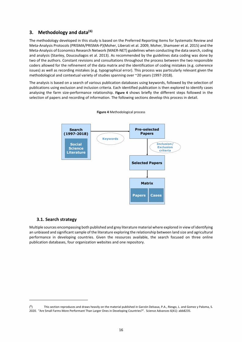
The analysis is based on a search of various publication databases using keywords, followed by the selection of publications using exclusion and inclusion criteria. Each identified publication is then explored to identify cases analysing the farm size-performance relationship. Figure 4 shows briefly the different steps followed in the selection of papers and recording of information. The following sections develop this process in detail.

Figure 4 Methodological process

3.1. Search strategy Multiple sources encompassing both published and grey literature material where explored in view of identifying an unbiased and significant sample of the literature exploring the relationship between land size and agricultural performance in developing countries. Given the resources available, the search focused on three online publication databases, four organization websites and one repository.

(6) This section reproduces and draws heavily on the material published in Garzón Delvaux, P.A., Riesgo, L. and Gomez y Paloma, S. 2020. "Are Small Farms More Performant Than Larger Ones in Developing Countries?". Science Advances 6(41): abb8235.

Pre-selectedPapers

Selected Papers

Search(1997-2018)

SocialScience

Literature

Keywords

Inclusion/Exclusion criteria

Matrix

Papers Cases

17

Table 2 lists the sources. The peer-reviewed literature was completed by working papers from selected international development organizations and agricultural economics as well as material identified through snowballing.

Table 2 Data sources

Type Source Website

Online publication database SCOPUS http://www.scopus.com

CAIRN https://www.cairn.info/

Selected organization's publications

CIRAD (Agritrop) http://agritrop.cirad.fr/

FAO http://www.fao.org/publications/en/

IFPRI http://www.ifpri.org/publications

World Bank https://openknowledge.worldbank.org/

Repository Hal https://hal.archives-ouvertes.fr/

Individual references Snowball n/a

SCOPUS was identified as a more suitable database than Web of Science as they mostly overlaps, and Scopus supersedes it in the Social Sciences literature (Mongeon and Paul-Hus 2016), our main source of interest in this review.

Definitive searches were conducted between January and September 2019 updating initial and reference searches conducted in 2017 and 2018 to fully cover the 1997-2018 period.

3.2. Chosen controls in searching An important decision in the paper search criteria is to look beyond the specialised literature having focused on the land size-agricultural performance relationship by also searching into general agricultural and development economics literature having analysed such relationship. This greatly widens the scope of the review but more adequately responds to the need of developing the review. In addition, it allows partially controlling for a possible specificity associated to the specialised literature.

3.3. Search terms The initial scoping exercise consisted in identifying relevant search terms for both the specialised literature and the broader literature. The result of this initial set of search terms was the basis for the construction of the main library of relevant references.

18

Initial successive searches in SCOPUS are the result of the following combination of keywords:

Box 2 Combination of keywords for searching material in SCOPUS*

"inverse relationship" AND "agriculture"

"size productivity relationship"

"yields" AND "agriculture" AND "land" AND "size" OR "area"

"farm" AND "productivity"

"Ricardian" AND "climate change"

"net crop revenue"

"performance" AND "farm"

"performance" AND "agriculture"

"efficiency" AND "agriculture"

* "environmental indicator" AND "agriculture" Also included as part of the original search. Not pursed in the final

analysis.

Based on the combination of keywords showed in Box 2, three final sets of search strings were used for SCOPUS, the main source for both the specialised and broader literature. Such search strings were identified conducting a test against known key references from the first search including the following reference authors: Barrett, C.B.; Benjamin, D.; Carletto, G.; Collier, P; Dercon, S., Deininger, K.; Gollin, D.; Helfand, S.M.; Jayne, T.; Lamb, R.L.; Otsuka, K.; Rozelle, S.

Regarding the first set of the main terms, the following combination of keywords was introduced:

− "agricult*" OR "farm" OR "plot" OR "parcel" OR "area" OR "land" AND "inverse" AND "relationship"

The second set of main terms includes the following keywords:

− "agricult*" OR "farm" OR "plot" OR "parcel" OR "area" OR "land"

The search was also focused on the different type of indicators that can be found in the literature, as the following:

− "revenue" OR "income" OR "yield" OR "value" OR "efficiency" OR "productivity" OR "production" OR "profit" OR "rent" OR "performance"

In addition, some approach terms were included to identify different methodologies of analyses:

− "production function" OR "ricardian" OR "stochastic" OR "frontier" OR "DEA" OR "regression"

In opposition to the precise geographical classification of documents that can be found in institutional databases (e.g. World Bank, IFPRI), SCOPUS has a less functional metadata system(7). To address this, two identical

(7) Web of Science does not fare better, following testing.

19

searches were conducted, first using the metadata and excluding the irrelevant countries(8) and secondly including in the search string the individual names of countries in English. The full list is available in Annex III.

The results from the successive initial searches and the definitive search strings were merged so to have a more effective geographical coverage of the sources.

The search exploring the institutional databases in English used the following terms successively assuming that institutional repositories perform better with simpler search strings, as shown in Box 3.

Box 3 Combination of keywords for searching material in institutional databases

"land" AND "size" OR "area" OR "plot" OR "parcel" OR "surface"

"yields"

"inverse relationship"

"farm productivity"

"ricardian" AND "climate change"

The organisational databases offered the possibility to also select with precision the region from the metadata of documents; hence the focus of the searches was restricted to the macro region of interest or individual countries when possible.

In turn, the search exploring French databases and institutions was constructed, using the terms specified in Box 4.

Box 4 Combination of keywords for searching material in French

"taille " ET "exploitation agricole"

"relation inverse"

ET "agri*"

"Cobb Douglas" OU "frontière de production"

OU "fonction de production"

OU "efficacité technique"

OU "rendements"

ET "agri*"

"productivité" ET "terre"

"ricardien" ET " changement climatique "

(8) For the metadata on geographical location, a simple search with "agri*" was generated to produce the most complete list of options before engaging with the search string of interest.

20

When needed, a string of the individual names of the countries of interest was also included in the search in French.

Although the search was performed using keywords in English and French, the analysis included papers in English, French, Spanish, Portuguese and Italian. It is worth mentioning that the searching process analyses titles and abstracts that contains the keywords (or a combination), and the journals in Scopus always include information of titles and abstracts in both, the original publication language and English.

3.4. Screening Following the searches, lists of papers with the titles and at times with the paper abstract, were initially screened. Then, the papers appearing to meet the basic criteria were examined in their entirety to confirm that they actually met a number of inclusion criteria. This basic inclusion criteria includes issues such the use of econometric approaches matching a given performance indicator and crop area (where it farm, parcel or plot). Detailed description of the criteria for inclusion (and exclusion) of papers can be found in the following section.

Screening and consequent recording of the relevant information were made in close coordination and consultation (especially when facing difficult of ambiguous material) between the two main researchers. The check-up process proceeded continuously as researchers collaborated side by side.

3.5. Inclusion and exclusion criteria The inclusion of a given paper was determined by a pre-established set of inclusion and exclusion criteria as listed in Table 3.

Table 3 Inclusion and exclusion criteria

Inclusion Exclusion

Type of publication

Peer-reviewed papers, published books, working papers of selected organisations or papers from snowball identification

Unpublished material, theses in repositories, working or conference papers not meeting the inclusion criteria.

Years of publication

Papers published from 1997 to 2018 (both years included).

Publication dating from 1996 or before. No exclusion criteria for year of data used in publication. Key previous publications are referred to in the introduction and feed the interpretation, though.

Nature of analysis

Regression analyses. Any econometric approach with a performance indicator as dependant variable and at least land size as independent variable.

Descriptive or narrative studies, commentaries, experiments, trials, simulation or model, summaries or meta-analysis (this last type was used for snowball purposes, however).

Data Survey or census data at household / farm / parcel level.

Aggregated data beyond household or farm data (e.g. data of size at regional, national or supranational levels).

Scope Crop farm, Mixed farms, crop parcels/plots.

Cattle, dairy, aquatic or animal husbandry production systems (e.g. pure pastoral systems)

Performance indicators (*)

Gross Output (total production, total revenue, yield, value per area), Net Value (ratio revenues/cost, total profit, gross margin, net farm income, profit

Performance indicator on differentials (e.g. gap on productivity)

21

per area, gross margin per area, net farm income per area), Efficiency (technical, economic, etc. and TFP)

Explanatory variables (at least)

plot / farm / parcel / area / land size

Populations Developing countries, including most BRICS

Developed countries, including Russia, Armenia, Belarus, Moldavia, Taiwan, South Korea, Mauritius, West Indian European or American dominions

Languages English, French, Spanish, Portuguese, Italian

Other languages such as Mandarin, Japanese or Hindi

(*) Environmental indicators using as proxy of the adoption of soil and water conservation measures, including tree planting were explored in the screening of the literature. Given the heterogeneity, sparse evidence of actual environmental performance, we decided to exclude them from the analysis. In addition, the variety of crops recorded was also identified as a possible indicator of sustainability but the general paucity of the description of farm systems prevented such an analysis. The average number of crops in a single farms or plots are very rarely recorded, with only usually a single man crop recorded.

Including studies using econometric approaches is the main inclusion criteria. Econometric studies allow to capture the correlation between land size and the performance indicator alongside other control variables. Such approach reduces the need for researchers ´judgement (i.e. the use of descriptive statistics for a given range of farm sizes/typologies of farms does not imply any relationship between the size of the farm and the performance indicator). The main advantage of selecting econometric analyses is that a coefficient that shows the association between a performance indicator and land size is given, so the interpretation is transparent. Conversely, in the studies without econometrics, the analysis can only be completed by the author(s)' judgment, which consequently is less transparent.

Another criterion to consider is the number of approaches used to understand and measure the farm size or rather the scale of agricultural operation. The present analysis focuses on land area rather than scale indicators. This choice is motivated by data limitations and it is in line with the findings of Eastwood et al (2010). Indeed, they show that strong correlations exist between alternative indicators of scale and land area. Furthermore, this choice enables feeding into the current debates on studies exploiting land area variables The expression "size of farm" (or plot/parcel, when relevant) is used interchangeably to land area here.

3.6. Sampling unit and unit of analysis The initial sampling units for the search are individual publications or papers. However, the unit of analysis is that of observations or cases within each paper. A single paper may offer insights as to various cases but also explore them through different approaches. As illustration, Figure 5 provides the following example. A given paper may produce 4 different cases, namely 1 for the whole country, a second for one region of the country and a third for another region of the same country. In addition, the paper uses two different approaches (i.e. functional forms) to assess the effect of the land size on the performance indicator at country level. For the review, three cases would have been selected: those corresponding to the two regions and the whole country analysis having used the method identified by the author of the paper as the most appropriate to the analysis (functional form 1 in the example). An illustration of the matrix is presented in Annex III.

22

Figure 5 Sampling and analysis units

This approach allows extracting the different cases that a paper identifies while avoiding duplication of cases simply because of an alternative specification of the model.

3.7. Study coding strategy The information gathered was recorded in a unified matrix resulting from a pre-established structure which was adapted when recording the first 50 papers (and associated cases) so to adapt it to the existing material.

The final version matrix has over 570 columns, gathering information for all cases extracted from the papers under the following 13 broad categories of data:

− Paper and case ID.

− Bibliographic information, including whether peer-reviewed, published in an impact factor journal in Web of Science, impact factor in Scopus, journal rank in the journal category in Scopus and specificity(9) of the paper in the literature.

− Type of relationship between the performance indicator and the land size (i.e. direct, inverse or non-monotonic relationship), and significance of such relationship.

− Information on the scope of the land analysis: farm /plot level.

− Selection of the case for final analysis (see sections 3.5 and 3.6 for more details).

− Indicators for agricultural performance.

− Crops and crop group.

− Typology (Agro-Ecological Zone (AEZ), Farming systems).

− Contextual variables of the country at time of data collection (e.g. proportion of active population in agriculture, rural population density, etc.)

− Variables included in the analysis to explain the land-performance relationship, and if significant.

− Sample size.

− Land size distribution.

− Methodological approach.

− Summary of control variables (e.g. soil quality, labour, credit, etc.).

3.8. Data analysis and synthesis Data extracted from each article was compiled into the matrix as described above and made available for analysis. The analysis consists of a description of the data gathered through graphs, descriptive statistics and bivariate tests. Existing reviews have highlighted historical weaknesses of the literature on IR pointing to methodological shortcomings. This calls for the introduction of quality checks to ensure the robustness of this current review spanning over a wide time span and literature.

(9) By specificity of the paper in the literature we understand those papers that are focused on the analysis of the potential Direct/IR/non-monotonicity in the relationship between land size and a performance indicator.

Paper 1 Region 1

Wholecountry

Region 2

Functional form 1

Functional form 2

Case 1

Case 1

Case 3

Case 2 SelectedCase 2

SelectedCase 3

SelectedCase 1

23

Shortcomings are particularly related to the nature of the performance indicator (i.e. partial productivity indicator embodied in simple yields or total value of production), unrefined or missing important control/contextual variables such as soil quality and a very limited range of farm sizes within a given study (e.g. only focusing on lands smaller than 5 ha).

At the level of a descriptive quantitative review, a way for controlling the effects of such methodological weaknesses is to present the main results of the relationship between land area and performance with data focusing on a selected number of criteria. One thing is the results emerging from the sample of cases as a whole yet another might be the evidence that comes from a selected subsample according to the following quality criteria:

− Papers from the last 10 years prior to 2018;

− Cases from papers published in Q1 and Q2 journals according to SCOPUS classification;

− Cases from specialised papers;

− Cases from specialised papers published in publications with impact factor;

− Cases with above median sample size of each indicator group;

− Cases according to data source, survey type and average farm category (e.g. <1Ha);

− Cases with cereals as the only main crop;

− Results emerging from the more advanced designed studies in terms of key control variables (soil quality, GPS, irrigation, record of off-farm activity, record of credit access, education and age of head of households) and specification of the relationship between land size and agricultural performance.

3.9. Limitations The limitations of the search exercise are threefold. The first is related to the search strategy and its scope. The ambitious geographical scope is not fully realised because of the inclusion of only a limited number of organisational repositories (i.e. World Bank, FAO, etc.). Regional development institutions such as the Asian, African and Inter-American Development Banks could be added in the future as well as other regional more academic repositories(10). However, such limitation only applies to publications without impact factor (IF) and, despite not directly searching the aforementioned institutional repositories, key publications were identified through snowballing.

Then, as it is mentioned before, the environmental performance was proxied following the initial review as the adoption of resource conservation measures (i.e. water and soil conservation techniques) given the paucity of alternatives fitting the approach followed here. Moreover, the review of this performance dimension was not completed given the material available and hence it is not reported here.

In a similar vein, the average number of crops in a single farms or plots are very rarely recorded, with only usually a single man crop recorded preventing controlling for the variety of crops recorded. Such information could be an indicator of sustainability and provide a wider view as to the FNS implications. However, although the detailed list of crops is not systematic, the total value of production is generally provided allowing for a relevant analysis.

Finally, some relevant papers may have not been correctly identified due to the language, especially in the case of China.

(10) Potential other sources were AGROBASE/BINAGRI, AGRIS/CARIS, BIBLIOTECA NACIONAL, IBICT/SEER, CAB ABSTRACTS (CABI - Commonwealth Agricultural Bureaux International), Redalyc and DOAJ (Directory of Open Access Journals).

24

4. Results

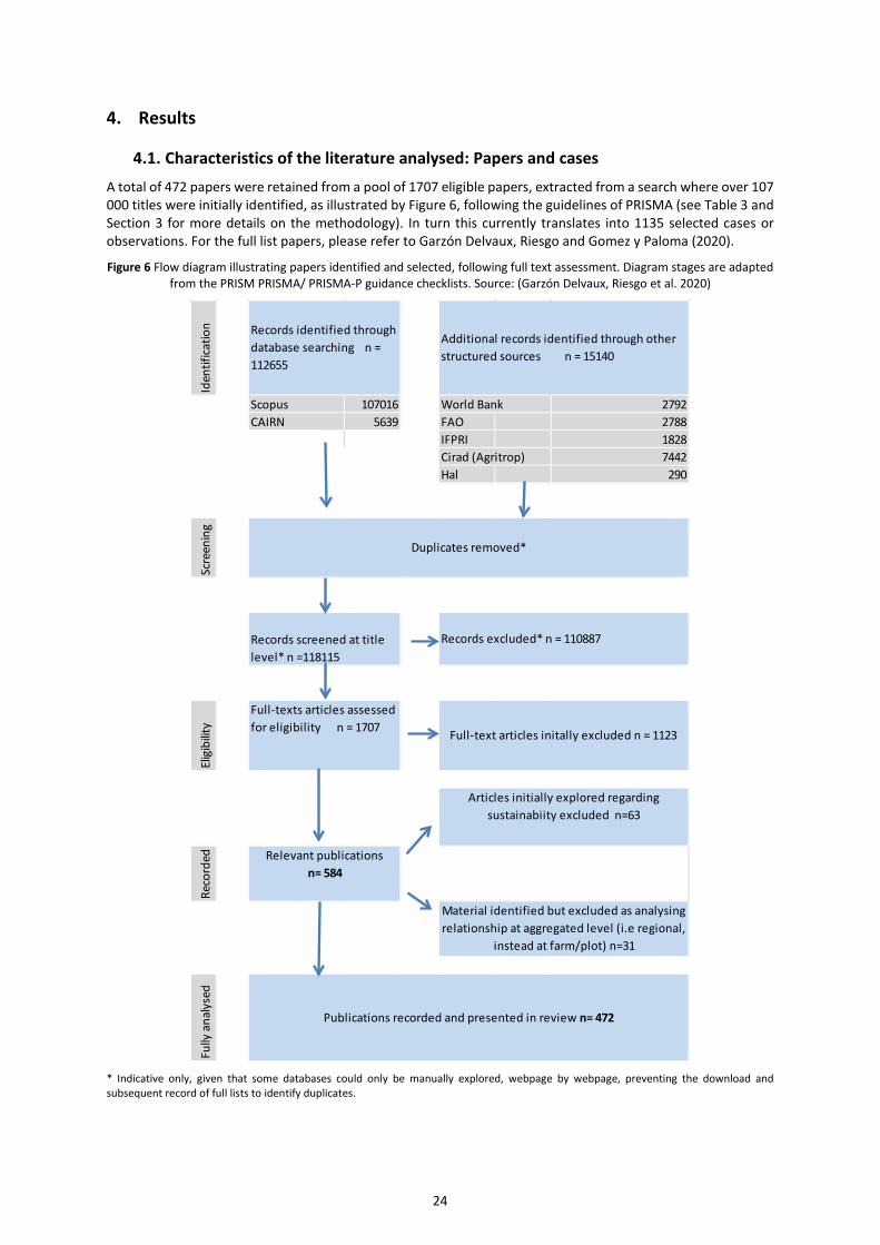
4.1. Characteristics of the literature analysed: Papers and casesA total of 472 papers were retained from a pool of 1707 eligible papers, extracted from a search where over 107 000 titles were initially identified, as illustrated by Figure 6, following the guidelines of PRISMA (see Table 3 and Section 3 for more details on the methodology). In turn this currently translates into 1135 selected cases or observations. For the full list papers, please refer to Garzón Delvaux, Riesgo and Gomez y Paloma (2020).

Figure 6 Flow diagram illustrating papers identified and selected, following full text assessment. Diagram stages are adapted from the PRISM PRISMA/ PRISMA-P guidance checklists. Source: (Garzón Delvaux, Riesgo et al. 2020)

* Indicative only, given that some databases could only be manually explored, webpage by webpage, preventing the download andsubsequent record of full lists to identify duplicates.

Iden

tifica

tion

Scopus 107016 World Bank 2792CAIRN 5639 FAO 2788

IFPRI 1828Cirad (Agritrop) 7442Hal 290

Scre

enin

gEl

igib

ility

Reco

rded

Fully

ana

lyse

d

Material identified but excluded as analysing relationship at aggregated level (i.e regional,

instead at farm/plot) n=31

Publications recorded and presented in review n= 472

Articles initially explored regarding sustainabiity excluded n=63

Records identified through database searching n = 112655

Additional records identified through other structured sources n = 15140

Records screened at title level* n =118115

Records excluded* n = 110887

Relevant publications n= 584

Full-texts articles assessed for eligibility n = 1707

Duplicates removed*

Full-text articles initally excluded n = 1123

25

The geographical distribution of papers is dominated by material analysing experiences from Sub-Saharan Africa and Asia and the Pacific, with 209 papers and around 500 case studies in each region (see Table 4 and Figure 7 for a detailed distribution of papers and cases).

Table 4 Distribution of papers and case studies by macro-region

Region Papers Case studies (observations)

n Percent (%) n Percent (%)

SSA 209 44.3 528 46.5

ASIA 209 44.3 477 42.0

MENA 19 4.0 42 3.7

LAC 35 7.4 88 7.8

TOTAL 472 100 1135 100

The maps in Figure 7, showing all cases, and in Figure 8, showing those cases from specialised literature, point at the prevalence of certain countries per region. This is particularly the case with Ethiopia, Uganda, Nigeria and Kenya for Sub-Saharan Africa, as well as China and India in Asia. Such representations are important as they unveil a literature with the desired characteristics (please refer to the exclusion/inclusions criteria in Table 3) which is spatially concentrated. This is something which has been also identified in other research contexts for example in publications on African politics (Briggs 2017).

Figure 7 Map of the distribution of cases selected

26

Figure 8 Map of the distribution of cases selected, specialised papers only

The distribution of papers mainly covers cases in low and lower-middle income countries, according to the World Bank Income per capita classification, accounting for around 88% of the sample (see Table 5). By contrast, only 12% and 0.5% of the cases are related to upper-middle and high-income countries (e.g.: Chile, Saudi Arabia or South Africa).

Table 5 Distribution of papers and case studies by World Bank income classification

World Bank Income per capita(*) classification

Papers Case studies (observations)

n Percent (%) n Percent (%)

Low income,

L (<US$995) 247 53.5 605 54.9

Lower middle income, LM (US$996 - 3945) 157 34.0 363 32.9

Upper middle income, UM (US$3946 - 12195) 56 12.1 130 11.8

High income,

H (>US$12196) 2 0.4 5 0.5

TOTAL (**) 462 100 1103 100

(*) Annually updated threshold of the nominal gross national income (GNI) per capita in US$ (World Bank 2019) ( 11). (**)The difference of papers/cases in Table 4 and 5 is due to the cases before 1987 that were not classified by the World Bank at the time.

(11) In calculating GNI (formerly referred to as GNP) in U.S. dollars for certain operational and analytical purposes, the World Bank uses the Atlas conversion factor instead of simple exchange rates. The purpose of the Atlas conversion factor is to reduce the impact of exchange rate fluctuations in the cross-country comparison of national incomes. The Atlas conversion factor for any year is the average of a country’s exchange rate for that year and its exchange rates for the two preceding years, adjusted for the difference between the rate of inflation in the country and international inflation; the objective of the adjustment is to reduce any changes to the exchange rate caused by inflation (World Bank, 2019).

27

Looking at the original data used in each paper, more than 1 million farms have been analysed by the review (see Total_1 in Table 6). Most of the farms are in Asia (52.4%), in particular in China and India, followed by SSA (31.6%).

As it is included in Table 6 (see Total_2 data) and Figure 9, it is worth mentioning that an exceptional study on Brazil with almost 4.7 million farms which modifies both the number of studied farms and the distribution of the most-analysed regions.

Table 6 Distribution of farms included in collected papers and studies

Region Farmers surveyed SSA 339 777

ASIA 563 048

MENA 13 143

LAC1 159 387

TOTAL_1 1 075 355 LAC2 4 858 809 TOTAL_2 5 934 164

Figure 9 Total farms analysed in original studies

28

4.1.1. Bibliometrics: Literature characteristics

Looking at the publication date of the papers gathered in the analysis, the yearly publication rate has increased, particularly over the last 10 years on Sub-Saharan Africa and Asia (Figure 10). In MENA and LAC the number of papers per year is much lower. As it is expected, there is a time lag between the publication of the paper and the last year of data collection.

Figure 10 Number of papers and last year of data collected, by macro-region and year

A considerable percentage (22.1%) of the papers can be found in few journals focused on agricultural economics (i.e. Agricultural Economics, Journal of Agricultural Economics or American Journal of Agricultural Economics). The World Bank Policy Research Working Papers and World Development also account for a considerable number of papers (6.5% and 4.4% respectively).

Table 7 Ranking of publications with > 2 papers on the topic (294 papers)

Main Publications Papers Ranking Impact factor-SJR (2018)

Agricultural Economics 39 1 1.81

World Bank Policy Research Working

19 2 n/a

Journal of Agricultural Economics 16 3 1.10

World Development 13 4 2.25

Agrekon 11 5 0.22

American Journal of Agricultural

10 6 1.91

Food Policy 10 6 1.78

29

Environment and Development

9 7 0.77

Land Economics 8 8 1.21

Land Use Policy 8 8 1.41

Journal of Development Economics 7 9 3.43

Agricultural Systems 6 10 1.36

Applied Economics 6 10 0.50

IFPRI Discussion Paper 6 10 n/a

Journal of African Economies 6 10 0.57

Journal of Development Studies 6 10 1.00

NJAS - Wageningen Journal of Life

6 10 0.73

Agricultural Economics Czech 5 11 0.44

American Journal of Applied Sciences 5 11 0.16

China Agricultural Economic Review 5 11 0.44

Food Security 5 11 1.25

Indian Journal of Agricultural

5 11 0.14

Journal of Food, Agriculture and

5 11 0.13

Quarterly Journal of International

5 11 n/a

Sustainability 5 11 0.55

Ecological Economics 4 12 1.77

Journal of the Asia Pacific Economy 4 12 0.25

Outlook on Agriculture 4 12 0.36

Quarterly Journal of International

4 12 0.46

Pakistan Development Review 4 12 0.10

African Journal of Agricultural and

3 13 n/a

Agris on-line papers in Economics and

3 13 0.30

Asian Economic Journal 3 13 0.17

China Economic Review 3 13 0.28

Climate Change Economics 3 13 0.31

Climate and Development 3 13 1.04

Climatic Change 3 13 1.64

ESA Working paper 3 13 n/a

Economic Development and Cultural

3 13 2.17

Experimental Agriculture 3 13 0.62

Journal of International Development 3 13 0.74

Journal of the Saudi Society of

3 13 n/a

Levy Economics Institute of Bard

3 13 n/a

Paddy and Water Environment 3 13 0.48

Pakistan Journal of Agricultural

3 13 0.31

Économie rurale. Agricultures,

3 13 n/a

30

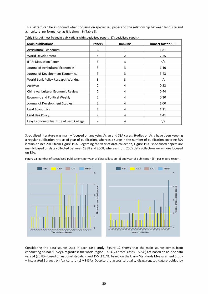
This pattern can be also found when focusing on specialised papers on the relationship between land size and agricultural performance, as it is shown in Table 8.

Table 8 List of most frequent publications with specialised papers (37 specialised papers)

Main publications Papers Ranking Impact factor-SJR Agricultural Economics 6 1 1.81

World Development 5 2 2.25

IFPRI Discussion Paper 3 3 n/a

Journal of Agricultural Economics 3 3 1.10

Journal of Development Economics 3 3 3.43

World Bank Policy Research Working

3 3 n/a

Agrekon 2 4 0.22

China Agricultural Economic Review 2 4 0.44

Economic and Political Weekly 2 4 0.30

Journal of Development Studies 2 4 1.00

Land Economics 2 4 1.21

Land Use Policy 2 4 1.41

Levy Economics Institute of Bard College 2 4 n/a

Specialised literature was mainly focused on analysing Asian and SSA cases. Studies on Asia have been keeping a regular publication rate as of year of publication, whereas a surge in the number of publication covering SSA is visible since 2013 from Figure 11-b. Regarding the year of data collection, Figure 11-a, specialised papers are mainly based on data collected between 1998 and 2008, whereas from 2005 data collection were more focused on SSA.

Figure 11 Number of specialised publications per year of data collection (a) and year of publication (b), per macro-region

Considering the data source used in each case study, Figure 12 shows that the main source comes from conducting ad-hoc surveys, regardless the world region. Thus, 737 total cases (65.5%) are based on ad-hoc data vs. 234 (20.8%) based on national statistics, and 155 (13.7%) based on the Living Standards Measurement Study – Integrated Surveys on Agriculture (LSMS-ISA). Despite the access to quality disaggregated data provided by

31

LSMS-ISA databases for 8 SSA countries, most of the analysed cases in this region use data from ad-hoc surveys (322 total cases using ad-hoc surveys vs. 108 cases using LSMS-ISA).

Figure 12 Distribution of selected cases, per macro-region and per data source

However, despite the importance of LSMS-ISA to provide datasets, most of the selected cases analysed in this study are based on ad-hoc surveys (65.5%). It is relevant to highlight, however, that the sample size of such ad-hoc surveys tends to be, in average, significantly smaller than for LSMS-ISA surveys or routine national surveys (see Table 9).

Table 9 Sample size of studies according to data source

Data source n Mean

(median) s.d. Min. Max.

LSMS 155 3 912.2

(2 212) 4 262.7 71 18 410

National statistics 234 4 510

(2 056) 433 230.9 36 4 699 422

Ad-hoc surveys 737 867.1

(243) 3 397.9 12 62 036

4.1.2. Bibliometrics: land size

As mentioned, land size in the literature is assessed through the measure of farms or plots. Analysing the average size of farms show some disparities between Asia and SSA (FAO 2002). The former has a mean farm size of 2. 58

0 20 40 60 80 100Percentage of cases selected

MENA

ASIA

LAC

SSA

LSMS National Statistics Ad-hoc surveys

0 200 400 600 800Number of cases selected

Ad-hoc surveys

National Statistics

LSMS

SSA LAC ASIA MENA

32

ha (excluding South Africa) whereas in Asia the size is slightly larger, around 3 ha (3.19 ha). This small disparity also holds looking at the median value (50% of farms are above and below this value), as farm size in both macro-regions are similar (1.58 ha in SSA vs. 1.18 ha in Asia). By contrast, farm size in LAC and MENA is much larger on average (9.28 ha in LAC excluding Brazil, and 8.16 ha in MENA) when compared to SSA or Asia.

Table 10 Summary statistics of land size of farms and plots, for selected cases per world macro-region, in hectares

Farms (ha) n Mean (median)

s.d. Min. Max.

ASIA 307 3.19

(1.18)

15.92 0.03 260

SSA 300 11.42

(1.65)

88.85 0.04 1 074

SSA (-South Africa)** 285 2.58

(1.58)

4.11 0.04 60.05

LAC 67 1 263

(9.68)

4 880 0.20 20 462

LAC (-Brazil)* 53 9.28

(9.68)

8.59 0.20 56.40

MENA 37 8.16

(5.1)

8.75 0.55 41.00

Plots (ha) n Mean

(median)

s.d. Min. Max.

ASIA 69 1.15

(0.4)

2.94 0.02 22.60

SSA*** 150 1.12

(0.8)

1.12 0.06 5.45

LAC 11 7.16

(4.5)

6.05 1.00 17.91

LAC (-Brazil)* 10 7.77

(6.1)

6.00 1.00 17.91

MENA 2 3.48

(3.48)

1.73 2.26 4.70

(*)LAC (-Brazil) refers to those data of LAC excluding those cases referred to Brazil. (**)SSA (-South Africa) refers to descriptive data of SSA excluding those cases referred to South Africa. (***) no cases for South Africa

The small differences on farm size disappear when analysing plot average size in SSA and Asia (close to 1.1 ha in both cases).

33

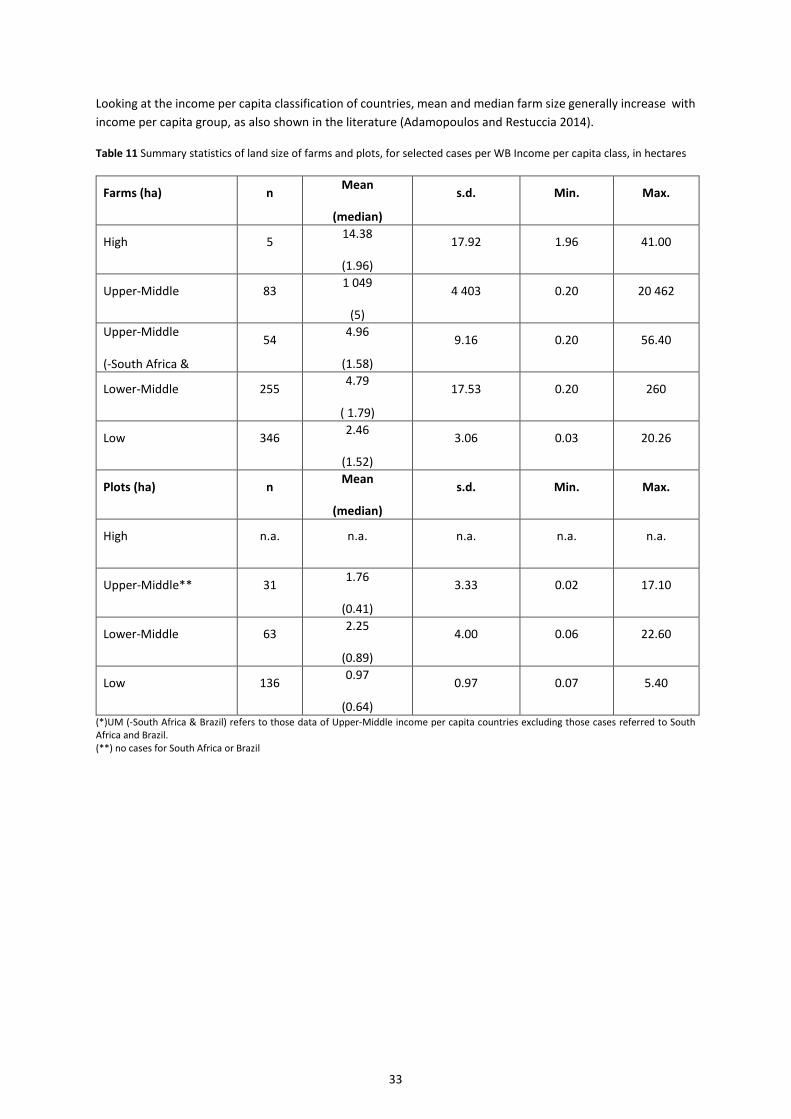
Looking at the income per capita classification of countries, mean and median farm size generally increase with income per capita group, as also shown in the literature (Adamopoulos and Restuccia 2014).

Table 11 Summary statistics of land size of farms and plots, for selected cases per WB Income per capita class, in hectares

Farms (ha) n Mean

(median)

s.d. Min. Max.

High 5 14.38

(1.96)

17.92 1.96 41.00

Upper-Middle 83 1 049

(5)

4 403 0.20 20 462

Upper-Middle

(-South Africa &

54 4.96

(1.58)

9.16 0.20 56.40

Lower-Middle 255 4.79

( 1.79)

17.53 0.20 260

Low 346 2.46

(1.52)

3.06 0.03 20.26

Plots (ha) n Mean

(median)

s.d. Min. Max.

High n.a. n.a. n.a. n.a. n.a.

Upper-Middle** 31 1.76

(0.41)

3.33 0.02 17.10

Lower-Middle 63 2.25

(0.89)

4.00 0.06 22.60

Low 136 0.97

(0.64)

0.97 0.07 5.40

(*)UM (-South Africa & Brazil) refers to those data of Upper-Middle income per capita countries excluding those cases referred to South Africa and Brazil. (**) no cases for South Africa or Brazil

34

4.1.3. Bibliometrics: agricultural performance indicators

When dividing the material into the three groups of agricultural performance indicators (i.e. gross output, net value and efficiency), gross output is the main focus of the analysis, with more than 398 selected cases in SSA and 280 in Asia (see Figure 13), mostly at farm level. Even in LAC and MENA, gross output is the main group of indicators considered to assess agricultural performance, but with a lower number of cases (57 and 22 cases respectively). One explanation for the extensive use of gross output indicators in the literature may be related to the ease of data collection (i.e. total production, and land size for yields). By contrast, the low use of net value indicators can be explained by the complexity of calculations. As it is mentioned in Section 1.3 it is required to assess some costs that are difficult to estimate (e.g. labour or opportunity costs), mainly in the presence of imperfect markets, as it happens in developing countries.

Figure 13 Selected cases according to whether the analysis was conducted at farm or plot level, by group of performance indicators and macro- region

When looking within each group of indicators, we can see that the four indicators (i.e. yields, total production, value per area and total revenue) used to assess the gross output are used in more or less the same proportion (Figure 14). For the other two groups (i.e. net value and efficiency), net farm income per area and efficiency indicators prevails (60 and 95% respectively).

0 20 40 60 80 100Percentage of cases selected

MENA

ASIA

LAC

SSA

Efficiency

Net value

Gross output

Efficiency

Net value

Gross output

Efficiency

Net value

Gross output

Efficiency

Net value

Gross output

Plot level Farm level

0 100 200 300 400Number of cases selected

y

e

t

y

e

t

y

e

t

y

e

t

35

Figure 14 Performance indicators analysed in the literature, in percentage and number of selected cases, by group indicator

0 20 40 60 80 100Percentage of cases selected

Efficiency

Net value

Gross output

Yield Total production Value per areaTotal revenue Ratio revenues/cost Profit per areaTotal profit Net farm income per area Total net farm incomeEfficiency analysis Total factor productivity (TFP)

0 200 400 600 800Number of cases selected

Efficiency

Net value

Gross output

36

4.1.4. Bibliometrics: agroecological zones (AEZ) coverage

Selected cases for the analysis are distributed across most of the existing agroecological zones offering an overview of conditions in tropical and sub-tropical areas, as shown in Figure 15.

Mixed AEZ refers to those cases that analyse the whole country or more than one AEZ, being impossible to classify them into a single AEZ, accounting for 23% of the sample. Another 23% of the cases are located in warm humid areas, being the most represented AEZ in the analysis.

Figure 15 Coverage of Agro-Ecological Zones (AEZ) by selected cases

4.1.5. Bibliometrics: crops covered by the analysis

Depending on the macro-region, crops produced are different but, not surprisingly, most of the selected cases focuses on cereals as the main crop group (over 55%), with maize predominating in SSA and rice doing so in Asia (Figure 16). Moreover, most mixed/undefined cases (25.11%) are also expected to be dominated by cereals despite the piecemeal background information made available for some studies. However, perennial crops (i.e. fruits, stimulants and other permanent crops) also make 7.40% of the sample as main crops, followed by fibre crops (4.14%) and vegetables (3.26%).

0 20 40 60 80 100Percentage of cases selected

Agro

-Eco

logi

cal Z

ones

(AEZ

)

Warm arid and semi-arid tropics Warm sub-humid tropics Warm humid tropics Highlands and subtropical cool Warm arid and semi-arid subtrop Warm sub-humid tropics (summer Warm/cool humid subtropics (sum Cool subtropics (summer rainfal Cool subtropics (winter rainfal Mixed AEZ

37

Figure 16 Selected cases, by main crop group

4.1.6. Bibliometrics: agricultural systems

Accounting for the sparse information on the agricultural systems covered by the studies, cases were classified according to the farming systems devised by Dixon et al. (2001) which combine bio-physical characteristics and crop/livestock systems. The figures below offer a perspective of the heterogeneity of situations present in the database for the main macro-regions, as distinguished by Dixon et al. (2001).

38

The most represented agricultural systems in SSA and Asia are related to the main crops adopted by farmers (Figure 17 and Figure 18). Therefore, the main agricultural system in SSA is characterised as maize mixed (around 17% of selected cases), whereas in Asia rice related systems are the majority (28% of rice-wheat and 16% of rice in South-East Asia, and more than 34% of lowland rice in East Asia and the Pacific).

Figure 17 Selected cases in SSA, by agricultural system

39

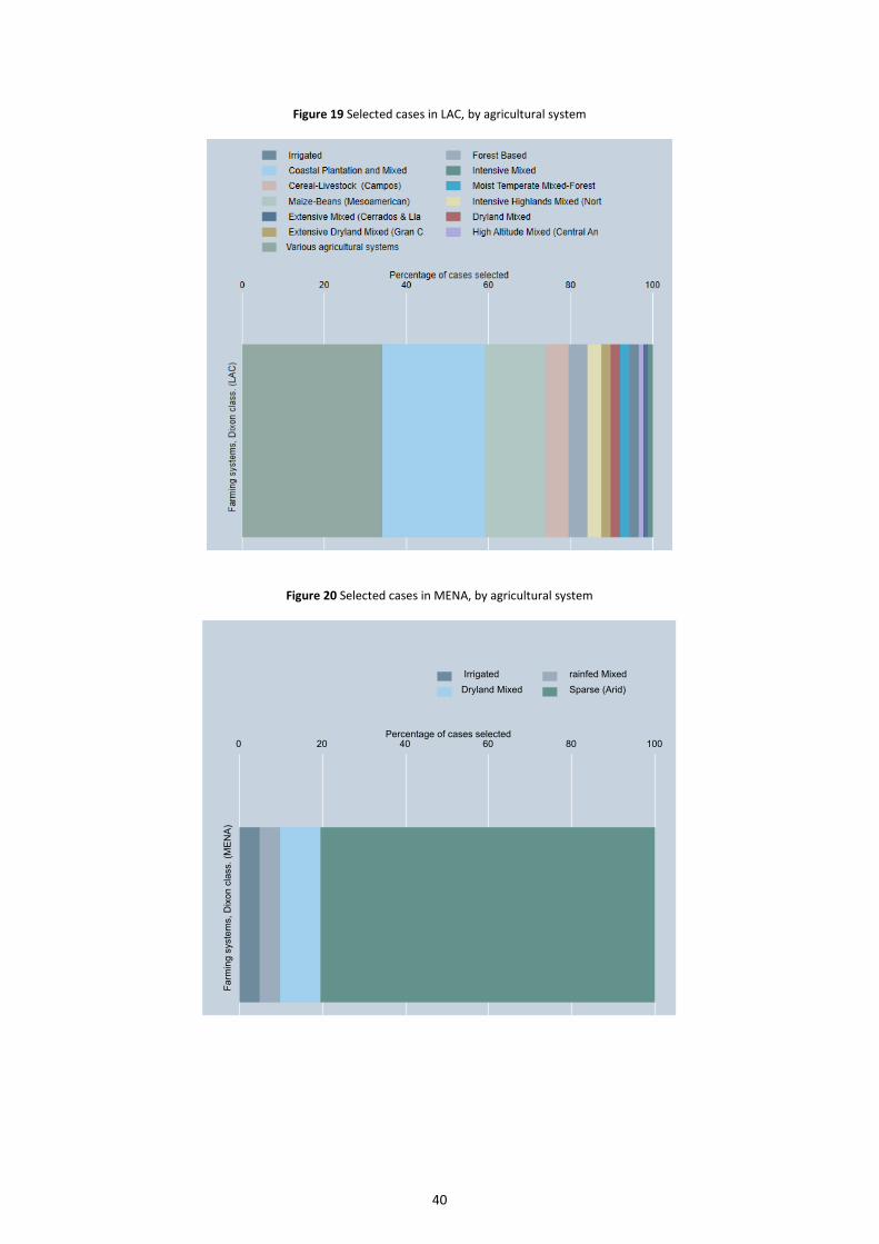
In LAC the coastal plantation and mixed categories is the most-analysed agricultural system in the sample with more than 25% of selected cases (Figure 19), followed by the maize-beans system (12%). Due to its geographical situation, the arid system is the main agricultural system in MENA, with around 80% of the selected cases (see Figure 20).

Figure 18 Selected cases in Asia, by agricultural system

40

Figure 19 Selected cases in LAC, by agricultural system

Figure 20 Selected cases in MENA, by agricultural system

0 20 40 60 80 100Percentage of cases selected

Farm

ing

syst

ems,

Dix

on c

lass

. (M

ENA)

Irrigated rainfed MixedDryland Mixed Sparse (Arid)

41

4.2. The relationship between land size and agricultural performance: Existing evidence

This section presents the results of the review on the land size-performance relationship according to the different performance indicators found in the literature (see Section 1.2 for the different relationships that can be found in the literature). Results are summarised into indicator groups (gross output, net value and efficiency), and are organised as follows. First, the results emerging from the whole sample of farm-level studies are analysed by macro-region (SSA, ASIA, LAC and MENA) and by World Bank per capita income classification (low (L), low-medium (LM), upper-medium (UM) and high (H)). The charts show both relative values (percentage) and absolute number of cases (frequency) in order to identify larger –and more meaningful- samples. Secondly, results are also presented for the studies developed at plot level, following the same structure.

Finally, the analyses are performed at farm level with a selection of quality, contextual and study-specific criteria proposed in Section 3.8 to test the robustness of the results and to control for potential biases introduced by the structure of the gathered sample and shortcomings identified by the literature.

4.2.1. The relationship between land size and agricultural performance: existing evidence at farm level

When looking at the whole sample of analysed literature by macro-region, the most striking element is the dominance of IR when analysing the gross output indicator group (see Figure 21 for macro-regions and Figure 22 for income per capita classification). A similar picture emerges by classifying cases according to the WB income-level classification and IR estimates in the context of low (L) and lower-medium (LM) are remarkably high with gross output analyses (~60%). By contrast, results are not so clear cut in favour of IR when analysing the other two indicator groups (Net Value and Efficiency). Moreover, for efficiency, analyses tend to estimate direct relationships (as area size grows, so does performance) in most of the macro-regions regardless their income classification.

Figure 21 Relationship results at farm level per performance indicator group, by macro-region, whole sample (selected cases)

0 20 40 60 80 100Percentage of selected cases

MENA

ASIA

LAC

SSA

Efficiency

Net value

Gross output

Efficiency

Net value

Gross output

Efficiency

Net value

Gross output

Efficiency

Net value

Gross output

Direct Inverse

Non-monotonic Non-significant

Size-performance relationship type:

0 50 100 150 200Number of selected cases

42

An important element in the results is provided by the alternative to IR and direct relationship since a non-negligible proportion of cases show a relationship which is non-monotonic (i.e. this relationship shows IR for small farm sizes and switch to direct relationship when the farm size increases, generally taking a U-shape). In addition, charts also show those cases in which the relationship may not be considered as statistically significant, so when no conclusions can be drawn.

Figure 22 Relationship results at farm level per performance indicator group, by WB class, whole sample (selected cases)

Focusing the analysis on the most-analysed macro-regions, SSA and Asia, we can see that the general trends observed for each region are maintained when looking at intraregional data by income classification (Figure 23 for SSA and Figure 24 for Asia).

Figure 23 Relationship results at farm level per performance indicator group, by WB class, SSA (selected cases)

0 20 40 60 80 100Percentage of selected cases

UM

LM

L

Efficiency

Net value

Gross output

Efficiency

Net value

Gross output

Efficiency

Net value

Gross output

Direct Inverse

Non-monotonic Non-significant

Size-performance relationship type (SSA):

0 50 100 150 200Number of selected cases

43

For both regions IR is the relationship that appears on most cases when gross output is used to measure agricultural performance, regardless the income level (i.e., low (L), lower-middle (LM) or upper-middle (UM) income levels). In SSA IR dominates in more than 60% of total cases using gross output as indicator, whereas in Asia is generally slightly lower, but still around 60%. This prevalence however vanishes in both regions when the indicator used is net value or efficiency.

Figure 24 Relationship results at farm level per performance indicator group, by WB class, Asia (selected cases)

In addition to the visual presentation of the results, bivariate tests(12) were performed to check the robustness of the association between a case showing a type of relationship (e.g. IR with respect to a direct relationship) and a performance indicator (e.g. gross output).

The largest samples (SSA and Asia at macro-region level, and low (L) and lower-middle (LM) at income level classification) show that IR is less frequent when using net value indicators than when using gross output, and when comparing efficiency and gross output indicators. Both results can be found in Table 12 showing a statistically significant negative sign (i.e. - sign) on the prevalence of IR when net value and gross output indicators are considered, and additionally when comparing efficiency and gross output indicators.

Table 12 Comparing the prevalence of IR estimations with respect to direct relationship between performance indicators, by macro- region and WB income class at farm-level, all sample, no filters.

Comparing the frequency of IR between groups of indicators *

Macro-region World Bank income classification

Indicators SSA LAC ASIA MENA H L LM UM

(12) Pearson Chi² and Cramer’s tests for categorical variables and t-test for continuous variables assuming unequal variances areconducted. Details are presented in Annexes.

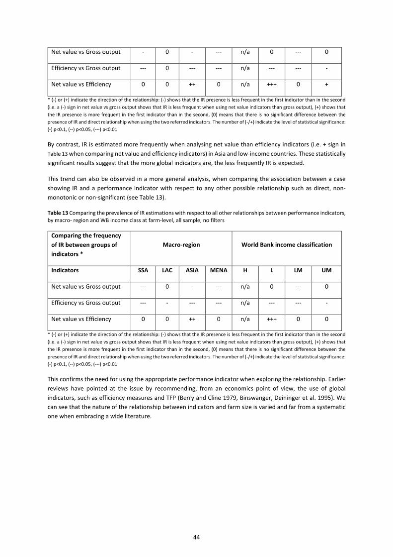
44

Net value vs Gross output - 0 - --- n/a 0 --- 0

Efficiency vs Gross output --- 0 --- --- n/a --- --- -

Net value vs Efficiency 0 0 ++ 0 n/a +++ 0 +

* (-) or (+) indicate the direction of the relationship: (-) shows that the IR presence is less frequent in the first indicator than in the second (i.e. a (-) sign in net value vs gross output shows that IR is less frequent when using net value indicators than gross output), (+) shows that the IR presence is more frequent in the first indicator than in the second, (0) means that there is no significant difference between the presence of IR and direct relationship when using the two referred indicators. The number of (-/+) indicate the level of statistical significance: (-) p<0.1, (--) p<0.05, (---) p<0.01

By contrast, IR is estimated more frequently when analysing net value than efficiency indicators (i.e. + sign in Table 13 when comparing net value and efficiency indicators) in Asia and low-income countries. These statistically significant results suggest that the more global indicators are, the less frequently IR is expected.

This trend can also be observed in a more general analysis, when comparing the association between a case showing IR and a performance indicator with respect to any other possible relationship such as direct, non-monotonic or non-significant (see Table 13).

Table 13 Comparing the prevalence of IR estimations with respect to all other relationships between performance indicators, by macro- region and WB income class at farm-level, all sample, no filters

Comparing the frequency of IR between groups of indicators *

Macro-region World Bank income classification

Indicators SSA LAC ASIA MENA H L LM UM

Net value vs Gross output --- 0 - --- n/a 0 --- 0

Efficiency vs Gross output --- - --- --- n/a --- --- -

Net value vs Efficiency 0 0 ++ 0 n/a +++ 0 0

* (-) or (+) indicate the direction of the relationship: (-) shows that the IR presence is less frequent in the first indicator than in the second (i.e. a (-) sign in net value vs gross output shows that IR is less frequent when using net value indicators than gross output), (+) shows that the IR presence is more frequent in the first indicator than in the second, (0) means that there is no significant difference between the presence of IR and direct relationship when using the two referred indicators. The number of (-/+) indicate the level of statistical significance: (-) p<0.1, (--) p<0.05, (---) p<0.01

This confirms the need for using the appropriate performance indicator when exploring the relationship. Earlier reviews have pointed at the issue by recommending, from an economics point of view, the use of global indicators, such as efficiency measures and TFP (Berry and Cline 1979, Binswanger, Deininger et al. 1995). We can see that the nature of the relationship between indicators and farm size is varied and far from a systematic one when embracing a wide literature.

45

Table 14 Comparing the prevalence of IR estimations with respect to direct relationship between performance indicators, by Agro-ecological zones (AEZ) at farm-level, all sample, no filters.

Comparing the frequency of IR between groups of indicators *

AEZ

Indicators

War

m a

rid a

nd se

mi-

arid

T.

War

m su

b-hu

mid

T.

War

m h

umid

T.

High

land

s and

sub-

T.

cool

T.

War

m a

rid a

nd se

mi-

arid

sub-

T. (µ

)

War

m su

b-hu

mid

T. (

µ)

War

m/c

ool h

umid

sub-

T.(µ

)

Cool

sub-

T. (µ

)

Cool

sub-

T.(©

)

Mix

ed A

EZ

Net value vs Gross output

-- --- 0 0 +++ 0 --- 0 --- 0

Efficiency vs Gross output

0 --- --- --- 0 n/a --- - --- --

Net value vs Efficiency

0 0 ++ 0 +++ n/a 0 0 n/a 0

T. indicates tropics, (µ) indicates summer rainfall, (©) indicates winter rainfall.* (-) or (+) indicate the direction of the relationship: (-) shows that the IR presence is less frequent in the first indicator than in the second(i.e. a (-) sign in net value vs gross output shows that IR is less frequent when using net value indicators than gross output), (+) shows that the IR presence is more frequent in the first indicator than in the second, (0) means that there is no significant difference between thepresence of IR and direct relationship when using the two referred indicators. The number of (-/+) indicate the level of statistical significance: (-) p<0.1, (--) p<0.05, (---) p<0.01

We perform the same analysis but considering the different AEZ (see Table 14) and the main crop of the study (Table 15). Results are quite similar, regardless the AEZ or the main crop analysed, those indicators related to net value and efficiency show lower prevalence of IR than gross output (i.e., negative sign when comparing net value vs gross output and efficiency vs gross output, shows that IR is less prevalent in the first indicator than in the second).

Table 15 Comparing the prevalence of IR estimations with respect to direct relationship between performance indicators, by main crop (FAO classification) at farm-level, all sample, no filters.

Comparing the frequency of IR between groups of indicators *

Indicators

Cere

als

Root

s & tu

bers

Suga

r cro

ps

Puls

es

Oil

crop

s

Vege

tabl

es

Frui

ts

Fibr

e cr

ops

Stim

ulan

ts

Mix

ed c

rops

Net value vs Gross output

- n/a n/a n/a n/a n/a n/a 0 n/a ---

Efficiency vs Gross output

--- -- - 0 0 -- -- 0 0 ---

Net value vs Efficiency

++ 0 0 n/a n/a 0 n/a 0 n/a 0

* (-) or (+) indicate the direction of the relationship: (-) shows that the IR presence is less frequent in the first indicator than in the second(i.e. a (-) sign in net value vs gross output shows that IR is less frequent when using net value indicators than gross output), (+) shows that

46

the IR presence is more frequent in the first indicator than in the second, (0) means that there is no significant difference between the presence of IR and direct relationship when using the two referred indicators. The number of (-/+) indicate the level of statistical significance: (-) p<0.1, (--) p<0.05, (---) p<0.01

Looking at the most-analysed macro-regions (Table 16, Table 17 and Table 18), we can see that for most of the farming systems we do not have enough evidence to compare all the different possibilities (i.e. n/a value in the table), but when possible the trend is being kept.

Table 16 Comparing the prevalence of IR estimations with respect to direct relationship between performance indicators, by farm system in SSA (Dixon et al. 2001) at farm-level, all sample, no filters.

Comparing IR freq. *

Farming system (SSA)

Indicators

Irrig

ated

Tree

cro

p

Fore

st b

ased

Rice

-Tre

e Cr

op

High

land

Per

enni

al

High

land

Tem

p. m

ixed

Root

Cro

p

Cere

al R

oot c

rop

mix

Mai

ze M

ixed

Com

mer

cial

Agro

-Pas

tora

l mill

et-

sorg

hum

Mix

ed

Net value vs Gross output

n/a n/a n/a n/a -- 0 n/a n/a 0 n/a n/a -

Efficiency vs Gross output

0 n/a 0 n/a n/a 0 0 - 0 n/a n/a ---

Net value vs Efficiency

n/a n/a n/a n/a n/a n/a n/a 0 0 n/a n/a 0

Table 17 Comparing the prevalence of IR estimations with respect to direct relationship between performance indicators, by farm system in ASIA, East-Asia and Pacific (Dixon et al. 2001) at farm-level, all sample, no filters.

Comparing IR freq. *

Farming system (ASIA, East Asia and Pacific)

Indicators

Low

land

Ric

e

Tree

Cro

p M

ixed

Root

–Tub

er

Upl

and

Inte

nsiv

e M

ixed

High

land

Ex

tens

ive

Mix

ed

Tem

pera

te

Mix

ed

Spar

se

(For

est)

Spar

se (A

rid)

Mix

ed

Net value vs Gross output

--- n/a n/a - n/a 0 n/a n/a 0

Efficiency vs Gross output

n/a n/a n/a n/a n/a n/a n/a n/a n/a

Net value vs Efficiency

0 n/a n/a 0 n/a n/a n/a n/a +++

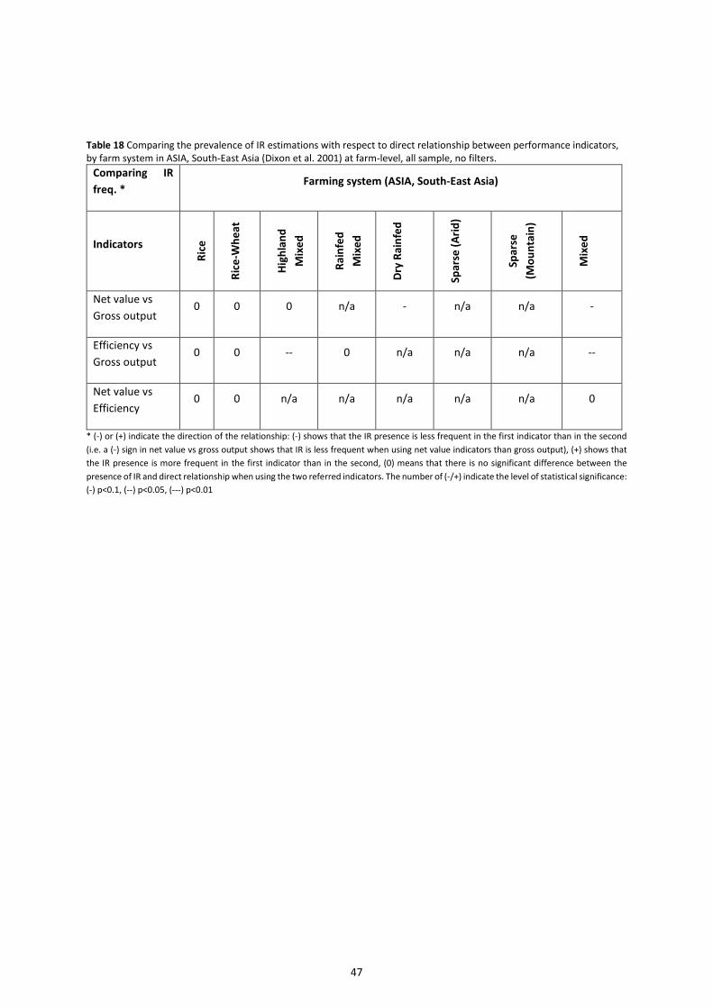
47

Table 18 Comparing the prevalence of IR estimations with respect to direct relationship between performance indicators, by farm system in ASIA, South-East Asia (Dixon et al. 2001) at farm-level, all sample, no filters.

Comparing IR freq. *

Farming system (ASIA, South-East Asia)

Indicators

Rice

Rice

-Whe

at

High

land

M

ixed

Rain

fed

Mix

ed

Dry

Rain

fed

Spar

se (A

rid)

Spar

se

(Mou

ntai

n)

Mix

ed

Net value vs Gross output

0 0 0 n/a - n/a n/a -

Efficiency vs Gross output

0 0 -- 0 n/a n/a n/a --

Net value vs Efficiency

0 0 n/a n/a n/a n/a n/a 0

* (-) or (+) indicate the direction of the relationship: (-) shows that the IR presence is less frequent in the first indicator than in the second (i.e. a (-) sign in net value vs gross output shows that IR is less frequent when using net value indicators than gross output), (+) shows that the IR presence is more frequent in the first indicator than in the second, (0) means that there is no significant difference between the presence of IR and direct relationship when using the two referred indicators. The number of (-/+) indicate the level of statistical significance: (-) p<0.1, (--) p<0.05, (---) p<0.01

48

Box 5 The farm size performance relationship: a view from the agricultural censuses and national accounts.

A bird's eye view of the latest available censuses point to an inverse relationship between the average size of farms and their mean gross value performance per hectare (Figure 25 (a)).

Figure 25 Gross product value (a), net value (b), and net value per worker (c) in agriculture, per hectare (log) and average farm size (log). Sources: (von Braun and Mirzabaev 2015, DANE 2016, Lowder, Skoet et al. 2016, FAO 2018, World Bank 2018)

Further looking at the relationship between farm size and agricultural performance, it is informative to assess the relationship of more global indicators which account for the costs involved in producing value. At aggregated level the net value per hectare does not seem to be associated to the mean size of farms (Figure 25 (b)). However, the net value produced per worker clearly rises with the average size of farms in censuses of the countries available (Figure 25 (c)). This last indicator is close to that of efficiency as it takes into account input costs and what is produced by a given factor of productivity (i.e. labour).

Such aggregated evidence closely matches the type of relationships that emerge from our review of individual cases.

ARG

GBR

USA

LUX

PRI

BEL

VIR

MLT

SWE

QAT

DEU

LBNNLD

DNK

URY

FRA

CHE

CAN

NORTTO

JORCYP

CZE

JPN

ITA

BHS

BRB

SVKAUT

EST

FIN

HUNESP

LBY

IRL

NZL

VCT

SVNASM

GUM

BGR PRT

VEN

PYF

CHLLVACOL

KOR

HRV

PAN

GRC

LTU

POL

DZA

JAM

BRA

IRN

LCAEGY

PRY

NIC

ECUHND

PHL

PER

GTM

TUR

ROUYEM MAR

SEN

CHN

PAKKGZIDN

CIV

FJI

THAIND

LSO

VNM

ALB

GINMMRNPLUGA

MOZ

LAO

ETH

MWI

COGGNB

BFA

DMA

WSM

KNAGRD

4

6

8

10

12

Gro

ss P

rodu

ct V

alue

per

hec

tare

(log

)

0 2 4 6Mean farm size in hectares (log)

n = 103

Gross Product value/ha (log) = 8.1305 - .29369 Mean farm size (log) R2 = 20.8%

ARG

GBR

PRI

MLT

SWE

QAT

DEU

LBN

NLD

DNK

URYFRA

CHE

CAN

NOR

TTO

JORCYPJPN

ITA

BHSBRB AUT

EST

FIN

HUN

ESP

LBY

IRL

NZL

ASM

GUM

BGR

PRT

PYF

CHL

LVA

COL

HRV

PAN

GRC

LTU

POL

DZA

JAM

BRAPRY

NIC

ECU

HND

PHL

PER

GTM

TUR

ROU

MAR

SEN

CHN

PAK

IDN

FJITHAIND

LSO

ALB

GIN

MMR

NPL

UGA

MOZETH

MWIGNB

BFA

DMA

WSM

GRD

6

7

8

9

10

Net

Val

ue p

er h

ecta

re (l

og)

0 2 4 6Mean farm size in hectares (log)

n = 77

Net Value per hectare (log) = 7.444 + .00374 Average farm size (log) R2 = 0.0%

GBR

PRI

MLT SWEDEU

NLDDNK URY

FRA

CHE

CAN

NOR

TTO

CYP

JPN

ITA

BHS

BRB

AUT

ESTFIN

HUNESP

IRL

NZL

BGRPRT CHL

LVAHRVPAN

GRC

LTUPOL

DZAJAM

BRA

PRY

NIC

ECU

PHL

PER

TUR

ROU

MAR

CHN

PAK

IDNTHAALB

6

8

10

12

14

Net v

alue

per

wor

ker (

log)

0 2 4 6Mean farm size in hectares (log)

n = 50

Net value per worker (log) = 7.8204 + .56296 Avergare farm size (log) R2 = 35.4%

49

4.2.2. The relationship between land size and agricultural performance: existing evidence at plot level

Focusing the analysis at plot level, the results are quite similar to those obtained at farm level when considering the gross output indicators (see Figure 26). Therefore, we can see that especially for SSA and in a lower extent for Asia, gross output indicators are the most frequently used in the literature. According to such indicators, IR appears as the main relationship between the size of the plot and the gross output (whether expressed in physical or monetary units). In Asia this trend is weaker, however.

Regarding net value indicators, IR also appears more frequently than a direct relationship in the remaining regions. When using efficiency indicators, this trend swaps towards a prevalence of direct relationship between plot size and performance.

Figure 26 Relationship results at plot level per performance indicator group, by macro-region, whole sample (selected cases, no filter).

When analysing the data by the WB income per capita classification (Figure 27), results are quite similar for low-income countries. However, when analysing low-medium and upper-medium countries, IR only prevails when using gross output indicators whereas a direct relationship dominates for the other indicator groups (i.e. net value and efficiency).

0 20 40 60 80 100Percentage of selected cases

MENA

ASIA

LAC

SSA

Efficiency

Net value

Gross output

Efficiency

Net value

Gross output

Efficiency

Net value

Gross output

Efficiency

Net value

Gross output

Direct Inverse

Non-monotonic Non-significant

Size-performance relationship type:

0 50 100 150Number of selected cases

50

Figure 27 Relationship results at plot level per performance indicator group, by WB income classification, whole sample (selected cases, no filter).

4.2.3. The relationship between farm size and agricultural performance: quality checks

As mentioned earlier (Section 3.8) the effects of any methodological issue on the relationship of farm size and agricultural performance is analysed using several quality criteria. In this section, we first test whether the results on the prevalence of IR between indicator groups obtained for the whole sample (see Section 4.2.1) holds when filtering by a number of quality variables, according to Figure 28. For example, we compare the results showing IR when using gross output indicators and when using net value for those publications issued by journals positioned on quartiles Q1 and Q2 of the SJR ranking, and afterwards we checked if such result coincided with the result for the whole sample (Table 19).

In addition to the visual presentation of the results, bivariate tests were performed to check the robustness of the association between a case showing a type of relationship (e.g. IR with respect to a direct relationship) and a performance indicator (e.g. gross output).

The largest samples (SSA and Asia at macro-region level, and low (L) and lower-middle (LM) at income level classification) show that IR is less frequent when using net value indicators than when using gross output, and when comparing efficiency and gross output indicators. Both results can be found in Table 19 showing a statistically significant negative sign (i.e. - sign) on the prevalence of IR when net value and gross output indicators are considered, and additionally when comparing efficiency and gross output indicators.

0 20 40 60 80 100Percentage of selected cases

UM

LM

L

Efficiency

Net value

Gross output

Efficiency

Net value

Gross output

Efficiency

Net value

Gross output

Direct Inverse

Non-monotonic Non-significant

Size-performance relationship type:

0 50 100Number of selected cases

51

Table 19 Comparing the prevalence of IR estimations with respect to direct relationship between performance indicators, by macro- region and WB income class at farm-level, all sample, no filters.

Comparing the frequency of IR between groups of indicators *

Macro-region World Bank income classification

Indicators SSA LAC ASIA MENA H L LM UM

Net value vs Gross output - 0 - --- n/a 0 --- 0

Efficiency vs Gross output --- 0 --- --- n/a --- --- -

Net value vs Efficiency 0 0 ++ 0 n/a +++ 0 +

* (-) or (+) indicate the direction of the relationship: (-) shows that the IR presence is less frequent in the first indicator than in the second (i.e. a (-) sign in net value vs gross output shows that IR is less frequent when using net value indicators than gross output), (+) shows that the IR presence is more frequent in the first indicator than in the second, (0) means that there is no significant difference between the presence of IR and direct relationship when using the two referred indicators. The number of (-/+) indicate the level of statistical significance: (-) p<0.1, (--) p<0.05, (---) p<0.01

By contrast, IR is estimated more frequently when analysing net value than efficiency indicators (i.e. + sign in Table 20when comparing net value and efficiency indicators) in Asia and low-income countries. These statistically significant results suggest that the more global indicators are, the less frequently IR is expected.

This trend can also be observed in a more general analysis, when comparing the association between a case showing IR and a performance indicator with respect to any other possible relationship such as direct, non-monotonic or non-significant (Table 20).

Table 20 Comparing the prevalence of IR estimations with respect to all other relationships between performance indicators, by macro- region and WB income class at farm-level, all sample, no filters

Comparing the frequency of IR between groups of indicators *

Macro-region World Bank income classification

Indicators SSA LAC ASIA MENA H L LM UM

Net value vs Gross output --- 0 - --- n/a 0 --- 0

Efficiency vs Gross output --- - --- --- n/a --- --- -

Net value vs Efficiency 0 0 ++ 0 n/a +++ 0 0

* (-) or (+) indicate the direction of the relationship: (-) shows that the IR presence is less frequent in the first indicator than in the second (i.e. a (-) sign in net value vs gross output shows that IR is less frequent when using net value indicators than gross output), (+) shows that the IR presence is more frequent in the first indicator than in the second, (0) means that there is no significant difference between the presence of IR and direct relationship when using the two referred indicators. The number of (-/+) indicate the level of statistical significance: (-) p<0.1, (--) p<0.05, (---) p<0.01

This confirms the need for using the appropriate performance indicator when exploring the relationship. Earlier reviews have pointed at the issue by recommending, from an economics point of view, the use of global indicators, such as efficiency measures and TFP (Berry and Cline 1979, Binswanger, Deininger et al. 1995). We can see that the nature of the relationship between indicators and farm size is varied and far from a systematic one when embracing a wide literature.

52

Figure 28. Tests for comparing results in subsamples based on quality checks

Filtering results by the selected quality variables confirms the association of IR to gross output indicators compared to Net value and Efficiency groups in most of the cases (i.e. negative relationship when comparing net value vs. gross output or efficiency vs. gross output in Table 21). However, some sub-samples do weaken the signal and may not identify any difference between indicators.

Table 21 Compared prevalence of IR estimation between performance indicator groups, according to selected sub-samples or quality filters, at farm level(13).

Macro regions WB income level classification

Filter Comparison SSA* LAC ASIA* MENA H L* LM* UM

Scopus Q1-Q2 journals

Net Value vs Gross --- 0 0 -- n/a 0 -- 0

Eff. vs Gross output --- 0 --- -- n/a --- --- --

Net value vs Eff. 0 0 +++ n/a n/a + + ++

Above median sample size normalised by indicator group

Net Value vs Gross 0 0 0 --- n/a 0 --- n/a

Eff. vs Gross output --- 0 --- --- n/a --- --- 0

Net value vs Eff. ++ 0 0 0 n/a +++ 0 n/a

Pre2008

Publication

Net Value vs Gross --- + - -- n/a -- --- n/a

Eff. vs Gross output --- 0 --- 0 n/a --- --- 0

Net value vs Eff. 0 ++ + 0 n/a 0 0 n/a

(13) This table only conduct tests on farm level studies, due to the small sample of plot level studies.

Whole sample

Gross output

Net value Effic.

Q1 & Q2(Gross output)

Q1 & Q2(Net value)

Test

Q1 & Q2Journals

Q1 & Q2Journals

53

Post2008

Publication

Net Value vs Gross 0 0 0 n/a n/a 0 --- 0

Eff. vs Gross output --- 0 --- --- n/a --- --- 0

Net value vs Eff. 0 0 + n/a n/a +++ 0 0

Specialised only

Net Value vs Gross --- 0 -- n/a n/a 0 --- n/a

Eff. vs Gross output --- 0 --- n/a n/a --- 0 ---

Net value vs Eff. ++ 0 + n/a n/a +++ -- n/a

Cereal, 1st crop group

Net Value vs Gross 0 0 - n/a n/a 0 --- 0

Eff. vs Gross output --- -- --- --- n/a --- --- 0

Net value vs Eff. 0 ++ 0 n/a n/a +++ 0 0

*Main focus of available evidence. Positive relationship at 0.1, 0.05 and 0.01 (+, ++, +++), meaning that IR is more prevalent in the first group of indicators than in the second (if Net Value vs. Eff, shows + for a specific filter, means that Net value indicators show IR more frequently than efficiency indicators, being such difference significant at 10%). Negative relationship at 0.1, 0.05 and 0.01 (-, --, ---), means that IR is more prevalent in the second group of indicators than in the first (if net value vs. gross output, shows - for a specific filter, this means that gross output indicators show IR more frequently than net value indicators, being such difference significant at 10%), 0: non-significant.

In particular, for those regions with higher number of observations (i.e. SSA and Asia and low and low-medium income countries), quality controls confirm that when using the more global (and recommended) indicators (i.e. net value, efficiency) IR is not the most common relationship between farm size and agricultural performance, questioning its ubiquity. This is particularly true when comparing results using efficiency vs gross output indicators. However, results not always show lower presence of IR when using net value than when gross output indicators are used. This is the case when the analysis is controlled by considering studies with a sample size above the median, those published after 2008 or analysing cereals as the main crop (Table 21). In these cases, tests results are not significant and consequently no conclusions can be drawn.

In a second step, results are compared by indicator, as it is shown in Figure 29. Therefore, results obtained in a quality subsample (e.g. results from journals ranked in first and second quartiles) are compared with results for the whole sample by each indicator group (see Table 22).

54

Figure 29 Tests comparing a quality subsample with the whole sample, by indicator

When analysing the introduction of quality filters in the sample, some results are worthy of a more detailed discussion.

Therefore, when using gross output indicators, specialised studies on the topic land size-agricultural performance relationship (i.e. those papers analysing specifically this key research question) show a higher prevalence of IR. This trend swaps for the other two groups of indicators: net value and efficiency, specialised papers show a lower presence of IR. Regarding the year of data collection, we can see that studies based on data collected after 2008 show a lower prevalence of IR. This might be explained since recent studies tend to use more sophisticated econometric models, and perhaps, such models using gross output indicators may better capture the nature of agricultural performance and land size.

Table 22 Association of quality variables to IR vs. direct relationship* Quality filters Gross output Net value Efficiency

Scopus Q1-Q2 Journals 0 ++ 0

Specialised papers +++ -- -

Data collected after 2008 --- 0 0

LSMS data +++ 0 0

Ad hoc survey data --- 0 0

National statistics data 0 0 0

* (-) or (+) indicate the direction of the relationship; the number of (-/+) indicate the level of statistical significance: (-) p<0.1, (--) p<0.05, (---) p<0.01

Finally, there is an impact of the data source on the prevalence of IR when using gross output indicators. Studies based on LSMS data show a higher prevalence of IR when compared with all the studies using gross output as

Gross output

Whole sample

Gross output

Net value Effic.

Test

Q1-Q2 jounals

55

performance indicator. By contrast, the use of ad-hoc surveys has the opposite effect, and results in a lower presence of IR when using gross output indicators. These results link with the question of limited land size range, and potentially invalidating a large share of the existing evidence as policy guidance as suggested by Collier and Dercon (2014). The larger the sample farm size range, the greater the possibility of capturing a direct relationship or a change in the relationship from IR to a direct relationship (Nkonde, Jayne et al. 2015, Muyanga and Jayne 2019). Thus, interpreting the relationship based on a sample of farms between 0.1 and 5 ha may not be interpreted with the same level of confidence as one encompassing wider ranges(14) which would combine marginal family holdings and larger ones as demonstrated by Muyanga and Jayne for Kenya (2019). Specifically-designed surveys to represent smallholders (e.g. LSMS) are more associated with IR than ad hoc ones, which can have different, wider sampling strategies.

4.2.4. The relationship between land size and agricultural performance: Choice and interpretation of indicators

One of the possible reasons why the literature has so often reported IR is related to misinterpretation. Exploring the "productivity of small versus larger farms" may be an ambiguous question, considering what is understood by productivity(15) and how it is estimated, leading in some cases to a misinterpretation of the implication of the type (and extent) of the relationship.

As it is mentioned on Section 1.3 there are different types of indicators which require adequate interpretation. One of the main group indicators used in the literature is gross output and is mainly related to total production and yields (physical amount of output or monetary units). It is important to consider that yields (or value per area), the most often used performance indicators (30% of the sample, and 45% of gross output indicators), are partial measures of productivity, and consequently only include one factor of production: land (Rada, Helfand et al. 2019). Hence, farm size-performance comparisons based on yields/value per area are short accounting for how farms of different sizes use all the other key factors of productions such as labour, fixed capital, and inputs.

By contrast, net value and efficiency indicators (e.g. profits, efficiency analyses) accounting for input and labour uses are preferable but seldom used (Berry and Cline 1979, Binswanger, Deininger et al. 1995, Helfand and Taylor 2017). When compared for the same sample, partial indicators (i.e. yields, value per area) tend to report IR while the more global indicators reject IR. Cases comparing gross output with global indicators can be found for various development regions (Cornia 1985), Ethiopia (Alene and Hassan 2003, Jote, Feleke et al. 2018), Nigeria (Aye and Mungatana 2011), Rwanda (Ali and Deininger 2015), Zimbabwe (Owens, Hoddinott et al. 2003), Nicaragua (Abdulai and Binder 2006, Henderson 2015), Turkey (Bozoğlu and Ceyhan 2007, Külekçi 2010), inter alia.

More comprehensive economic indicators of performance can be tested and may be both more powerful and better theoretically supported, in capturing the relationship in a meaningful way for policy (Kagin, Taylor et al. 2016, Helfand and Taylor 2017). Total factor productivity or efficiency analyses are better positioned to respond to the main question on whether smaller farms are more productive than larger ones. Moreover, and as reminded by Helfand and Taylor (2017), current analysis of the farm size-performance relationship in industrialised countries are more systematically done using efficiency and TFP indicators.

4.2.5. The relationship between land size and agricultural performance: Contextual variables

As briefly introduced, systematic farm size-performance relationship is expected from economic theory (Eastwood, Lipton et al. 2010, Scandizzo and Savastano 2017) but imperfection in labour, inputs, financial and/or

(14) Accounting for differences between crop land, mixed holdings and pure pastoral landholdings.(15) It is worth considering that analysis at (total) farm area and plot area level needs to be interpreted differently since theimplications are not the same.

56

land markets have critical implications. A strong candidate for the contextual explanation of a systematic IR in development context is that of labour market imperfections hypothesis, first introduced by Sen (1966).

Although imperfections in only one factor market is not sufficient to introduce a systematic relationship between farm size and performance, if two or more coalesce, such a relationship is expected, particularly IR (Binswanger, Deininger et al. 1995). For example, even if labour markets are imperfect but land markets do allow transfer of (at least) long-term user rights from land-abundant households to labour-abundant ones the relationship will not show IR(16). However, in most regions analysed neither labour nor land markets function efficiently, favouring the apparition of IR and limiting the performance of larger operation in relation to smallholders.

A fundamental mechanism is that when agricultural wage is sufficiently low (or almost null in given family labour circumstances), the family-labour-intensive agriculture is more competitive. Hence IR is observed with more efficient small-scale farms and inefficient large farms coexist. However, when alternative employment to farming emerge, wage rate increases limiting the initial advantage of smallholders and favouring the positioning of labour-saving method by the introduction of machinery, to the advantage of larger farms.

A contextualisation of the studies collected has been included in order to provide perspective to the analysis of results and most importantly to also test the main contextual hypotheses explaining the phenomenon of IR mainly that of rural input market imperfection(17).

IR is expected to be more prevalent among farming systems above a certain degree of rural population density. Although IR was historically pervasive in the literature mainly associated to Asia, its apparition in SSA is more recent and is associated with the gradual abandonment of slash-and-burn agriculture in favour of intensification agricultural practices, in turn due to the rise in rural population density (Otsuka, Liu et al. 2016). Since the pressure over land is stronger in densely populated rural communities, more numerous household members of farms are expected to face difficulties to increase their land size and consequently intensify their agricultural activity and production as much as possible. As intensification deepens, smallholders are expected to improve their land productivity, something recorded for Asia once the Green Revolution reached them following being adopted by the larger estates (Lipton 2009). Following Headay and Jayne (2014), rural areas are classified as land-constrained when the rural population density areas passes the threshold of 100 rural inhabitants by square kilometre (km²).

Demographic changes are captured by Figure 30 when comparing the context of the cases recorded in terms of rural population densities. Although SSA remains less densely populated than Asia, its density has increased over the years covered (1980-2017). The years (1980-2000) averaged rural population density to 380/km2 to reach 430/km2 in the following period (2000-2017).

(16) When one of the markets is competitive (and the production function is subject to constant returns to scale), an equally efficient allocation of resources among farms can be achieved in equilibrium. If labour markets work, labour-abundant but land-scarce householdswill work for land-abundant households. In turn if land markets operate (either as land sales or rent), labour-abundant households will either purchase or rent in land from land-abundant one Otsuka, K., Y. Liu and F. Yamauchi (2016). "Growing advantage of large farms in Asia andits implications for global food security." Global Food Security 11: 5-10.(17) Land market imperfection will be tested in the future. Other economic dimensions were tested but were inconclusive such asthe mean number of tractor/ha (data only updated until 2009), net capital stocks and stock formation in agriculture as well as averagefertilizer applied per area (kg/ha).

57

Figure 30 Distribution of cases according to the rural population density (inhabitants/km2), and data collection (before and after the year 2000)

Testing and matching rural population density per km² with the available data (FAOSTAT 2018) do not indicate a clear-cut land size-performance relationship direction. The existing signals were identified by testing the variable density both as a continuous and dichotomous variable using the land-constrained (100 inhabitants/ km² and 300 inhabitants/ km²) thresholds (Table 23), over the 1980-2000 period and the following one (2000-2017) (Table 24).

0

20

40

60

0

20

40

60

0 500 1000 1500 0 500 1000 1500

SSA LAC

ASIA MENA

Num

ber o

f sel

ecte

d ca

ses

Rural inhabitants per sq. kilomter (km2), before the year 2000

0

20

40

60

0

20

40

60

0 500 1000 1500 0 500 1000 1500

SSA LAC

ASIA MENA

Num

ber o

f sel

ecte

d ca

ses

Rural population per sq. kilometre (km2), after the year 2000.

58

Table 23 Comparing the prevalence of IR with respect to direct relationship between performance indicators, for all region, and by income class for SSA and Asia

All

cases SSA Asia

All L LM UM All L LM UM

Rural population density (continuous)

Gross output

0 0 0 +++ n/a 0 0 0 ++

Net value -- 0 0 n/a n/a -- + -- n/a

Efficiency 0 0 0 0 n/a 0 0 0 n/a

Rural population density > 100

Gross output

0 0 0 +++ n/a 0 0 0 0

Net value 0 0 0 n/a n/a n/a n/a n/a n/a

Efficiency 0 0 0 0 n/a 0 0 0 n/a

Rural population density >300

Gross output

0 0 0 n/a n/a 0 0 -- n/a

Net value 0 0 0 n/a n/a 0 0 0 n/a

Efficiency 0 0 0 n/a n/a 0 0 0 n/a

n/a: not application as the countries associated to such cases have average rural population densities above 100/km².

However, when focusing on LM income SSA countries, gross output cases seem to be confirming the association of an increasing density to IR, starting at 100 inhabitants per km² (Cameroon and Nigeria(18)), as hypothesised. Such an effect is suspected to be linked to the combination of land-constrained areas with market constrains, as showed in a recent review sourcing various surveys in 17 countries and covering 13 000 households (Frelat, Lopez-Ridaura et al. 2016). Such association is clearer for the data recorded since 2000. It is to be highlighted the association is not captured for the Low-income countries over the same period (2000-2017) or not conclusively recorded for the precedent period (1980-2000) either. Hence, IR could be more prevalent in the densely populated but transforming (having passed the Low-income category) contexts, may be materially allowing a more successful intensification by smallholders in terms of total production but not necessarily in terms of profitability or efficiency.

(18) The other countries of this income category below the density threshold for which cases were recoded are Ghana, Senegal and Gambia.

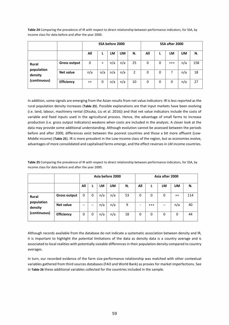
59

Table 24 Comparing the prevalence of IR with respect to direct relationship between performance indicators, for SSA, by income class for data before and after the year 2000.

SSA before 2000 SSA after 2000

All L LM UM N. All L LM UM N.

Rural population density (continuous)

Gross output 0 + n/a n/a 25 0 0 +++ n/a 158

Net value n/a n/a n/a n/a 2 0 0 ? n/a 18

Efficiency ++ 0 n/a n/a 10 0 0 0 n/a 27

In addition, some signals are emerging from the Asian results from net value indicators: IR is less reported as the rural population density increases (Table 25). Possible explanations are that input markets have been evolving (i.e. land, labour, machinery rental (Otsuka, Liu et al. 2016)) and that net value indicators include the costs of variable and fixed inputs used in the agricultural process. Hence, the advantage of small farms to increase production (i.e. gross output indicators) weakens when costs are included in the analysis. A closer look at the data may provide some additional understanding. Although evolution cannot be assessed between the periods before and after 2000, differences exist between the poorest countries and those a bit more affluent (Low-Middle income) (Table 25). IR is more prevalent in the Low-income class of the region, but as economies evolve, advantages of more consolidated and capitalised farms emerge, and the effect reverses in LM income countries.

Table 25 Comparing the prevalence of IR with respect to direct relationship between performance indicators, for SSA, by income class for data before and after the year 2000.

Asia before 2000 Asia after 2000

All L LM UM N. All L LM UM N.

Rural population density (continuous)

Gross output 0 0 n/a n/a 53 0 0 0 ++ 114

Net value -- -- n/a n/a 9 - +++ -- n/a 40

Efficiency 0 0 n/a n/a 18 0 0 0 0 44

Although records available from the database do not indicate a systematic association between density and IR, it is important to highlight the potential limitations of the data as density data is a country average and is associated to local realities with potentially sizeable differences in their population density compared to country averages.

In turn, our recorded evidence of the farm size-performance relationship was matched with other contextual variables gathered from third sources databases (FAO and World Bank) as proxies for market imperfections. See in Table 26 these additional variables collected for the countries included in the sample.

60

Table 26 Association of contextual variables to IR vs. direct relationship*

Contextual variables Gross output Net value Efficiency

Agricultural worker per agricultural area (ha) ++ 0 0

Share of active population in agriculture (%) 0 0 0

Share of agricultural GDP (%) 0 0 0

Arid and semi-arid, dummy 0 0 0

* (-) or (+) indicate the direction of the relationship: (-) means less IR, (+) more IR, (0) no significant difference; the number of (-/+) indicate the level of statistical significance: (-) p<0.1, (--) p<0.05, (---) p<0.01

Variables related to agricultural labour and associated wages such as agricultural worker per agricultural area or share of active population in agriculture show the level of dependence of the country on agriculture, and consequently the relative development of other sectors. High proportion of active population in agriculture points to limited employment opportunities for rural population beyond agriculture.

When conducted, actual testing of the impact of labour market imperfections on the farm size-performance relationship are conclusive. Illustrative examples of the effects of labour market imperfections were conducted for Pakistan (Heltberg 1998), Ethiopia (Holden, Shiferaw et al. 2001) and India (Deininger, Jin et al. 2016), concluding that where there are limited non-farming job opportunities IR is pervasive. In Kenya, other market imperfections also tested positive for IR, although not explaining all the recorded IR (Barrett, Bellemare et al. 2010).

In our review, labour-intensive agriculture (number of agricultural workers per hectare) is statistically significantly associated with IR reporting when gross output indicator is used as the indicator of agricultural performance. The other contextual variables do not seem to have any influence on the prevalence of IR, regardless the indicator group.

Finally, there seems to be no difference in the reporting of IR between cases in arid and semi-arid agroecological zones (AEZ) and other AEZ contexts, when using gross output and efficiency indicators. Although most cases report on a limited number of cereals, part of the sample should allow for enough variation, when testing the potential influence of the type of the main crops recorded, it does not seem to influence IR reporting.

4.2.6. The relationship between land size and agricultural performance: Methodological shortcomings

Besides the contextual explanations, the evidence gathered around the relationship was questioned given a series of methodological shortcomings dubbed to artificially result in IR from the analyses, feeding the debate surrounding both the inverse relationship and its policy implications (Collier and Dercon 2014). Simplistic models with missing key variables, such as soil quality or applied to a data sample with narrow range of smallholdings in their sample (Collier and Dercon 2014, Nkonde, Jayne et al. 2015) are suspected to unduly demonstrating that smaller holdings are more performant per area than larger farms, or at least exaggerate such difference.

Methodologically, these issues could be classified into two main groups as partially explaining the apparent ubiquity of the inverse relationship in developing countries. Here we group them as mismeasurement and misspecification which can affect estimates in a non-exclusive way.

61

Table 27 Association of explanatory variables to IR vs. direct relationship*

Explanatory variables Gross output Net Value Efficiency

GPS, dummy ++ 0 0

Soil quality and/or slope, dummy 0 ++ 0

Irrigation, dummy 0 - +

Off-farm activity, dummy --- 0 0

Credit imperfections, dummy 0 0 0

* (-) or (+) indicate the direction of the relationship: (-) means less IR, (+) more IR, (0) no significant differences; the number of (-/+) indicate the level of statistical significance: (-) p<0.1, (--) p<0.05, (---) p<0.01

As introduced earlier, some authors questioned the existence of IR in developing countries affirming that IR could only be the result of missing data on middle/large farms (Jayne, Chamberlin et al. 2016, Muyanga and Jayne 2019) or others as Carletto et al. (2013) raised a possible problem of mismeasurement. The literature has explored two main variables on both sides of the relationship, namely the possible effects of mismeasurement of the size of holdings(19) but also that of the volume of production (Carletto, Gourlay et al. 2015, Dillon, Gourlay et al. 2016, Desiere and Jolliffe 2017, Gourlay, Kilic et al. 2017). In the case of size of holdings, there seems to be a structural over-estimation of their size when only estimated and not precisely measured with GPS. The implications are that the intensity of IR is actually under-estimated in such circumstances. This is confirmed by the data as more precise land size measurement results in more recording of IR for gross output indicators studies, whereas it has no effect for the other indicator groups.

Independently of the measurement problems an additional dimension raised is that of the specification of the model. As occurred in any model, the variables included are also of importance to explain the results. One of the potential reasons to explain the (non) existence of IR is related to the variables used to explain such relationship. Therefore, we explore how the relationship between farm size and the agricultural performance behaves when the model to analyse such correlation includes other variables in its specification (i.e. the model to analyse the relationship between the performance indicator and the size of the farm usually includes more variables than only farm size. Such variables account for a number of issues such as socio-economic characteristics of the household, agricultural markets' characteristics, credit access, labour market, etc.). Theoretically, if a variable is not included in the model (e.g. access to credit) the rest of the variables might include part of the effect of such variable on the variable the model tries to explain (e.g. performance indicator) (20). By contrast, when a variable is included in the model its effect on the variable to explain is accounted

(19) Other questions surround measurement such as whether the estimates are of output per planted or harvested area Anderson, C. L., E. Slakie, T. Reynolds and M. K. Gugerty (2013). "Key Findings: Do Common Yield Measures Misrepresent Productivity Among Smallholder Farmers?: a Plot-level Analysis of Rice Yields in Tanzania." Evans School Policy Analysis and Research - EPAR Technical Report(252), Anderson, C. L. (2016). "Topics and Challenges in Agricultural Productivity Measurement." Ibid.(321). Also, the share of the area actually engaged in farming can created bias. Is it the whole farm, a fraction, or only a parcel which is assessed? For records of the evidence gathered for the review, farm size when the mention when all or most of the farm is assessed. Otherwise, estimates are classified as plot level analysis. (20) For instance, if there is a model where gross output is explained by only including farm size as an explanatory variable (𝑔𝑔𝑔𝑔𝑔𝑔𝑔𝑔𝑔𝑔 𝑔𝑔𝑜𝑜𝑜𝑜𝑜𝑜𝑜𝑜𝑜𝑜 = 𝛽𝛽0 + 𝛽𝛽1 ∙ 𝑓𝑓𝑓𝑓𝑔𝑔𝑓𝑓 𝑔𝑔𝑠𝑠𝑠𝑠𝑠𝑠), then other potential effects of the markets or the household are not accounted for in the model and as a consequence the coefficient of farm size (𝛽𝛽1) might not be realistic. If we introduce variables that may have an effect on the gross output, besides farm size, such as credit access (𝑔𝑔𝑔𝑔𝑔𝑔𝑔𝑔𝑔𝑔 𝑔𝑔𝑜𝑜𝑜𝑜𝑜𝑜𝑜𝑜𝑜𝑜 = 𝛽𝛽0 + 𝛽𝛽1 ∙ 𝑓𝑓𝑓𝑓𝑔𝑔𝑓𝑓 𝑔𝑔𝑠𝑠𝑠𝑠𝑠𝑠 + 𝛽𝛽2 ∙ 𝑐𝑐𝑔𝑔𝑠𝑠𝑐𝑐𝑠𝑠𝑜𝑜 𝑓𝑓𝑐𝑐𝑐𝑐𝑠𝑠𝑔𝑔𝑔𝑔), the coefficient of this latter variable (𝛽𝛽2) shows the effect of having/not having access to credit in the gross output, whereas the coefficient of farm size (𝛽𝛽1) does not include part of the effects of such difficulty to access to credit.

62

specifically, and consequently its effect is not included in other variables of the model. In turn, controlling for this aspect in the model specification was identified as a key parameter in explaining an apparent IR (Bhalla and Roy 1988, Lamb 2003): when including some variables the IR may not characterise agriculture in the estimates.

As mentioned before, some market imperfections may have an effect on the presence of IR. Looking at the results in Table 27, we can see that including variables related to off-farm activities results in reporting less IR using gross output indicators for all macro-regions (i.e. considering the full sample of observations). Since the existence of difficulties in labour markets is closely related to IR, it is expected that accounting for such imperfections in the models (i.e. including variables of market imperfections) results in reporting less IR.

Recording access to irrigation does not seem to capture any coherent or strong relationship with the incidence of IR, despite being an indicator of intensification.

Contrary to what some literature recommended (Bhalla and Roy 1988, Lamb 2003), including variables such as soil quality and/or slope of the land, only seem to have a coherent effect on IR reporting when compared to the rest of the studies not including such variables. This could be explained by both the questionable soil science robustness of the indicators used to account for soil quality in the model, and/or the inexistence of relevant differences in soil quality among the farms analysed in the studies (Barrett, Bellemare et al. 2010, Montanarella 2017).

4.2.7. The relationship between land size and agricultural performance: study specific variables

Socio-economic variables (Figure 31 for a graphical visualisation of the tests conducted on continuous variables) of the household may also explain some different behaviours, and as a consequence, different agricultural performance with respect to farm size, as shown by Table 28.

Figure 31 T-Tests comparing means of IR vs Direct results for specific continuous variables, by indicator

For example, the education level of farmers (i.e. number of schooling years) is lower on average, when IR is reported than when there is a direct relationship, if gross output indicators are used to analyse agricultural performance. The same applies for the average age of the head of the household: the average level of seniority of the head of the household is lower when IR is detected, using both gross output and net value indicators. In turn, studies having a very small average farm size among their sample (i.e. studies averaging farms <1 ha, very small subsistence farmers, representing 40% of all cases) do not seem to be specially associated with IR per se, however.

63

Table 28 Association of explanatory variables to IR vs. direct relationship*

Study specific variables Gross output Net Value Efficiency

Subsistence farms (mean farm size<1ha) 0 0 0

Years of education of HH head --- 0 -

Age of household head --- -- 0

* (-) or (+) indicate the direction of the relationship: (-) means less IR, (+) means more IR, (0) means no significant difference; the number of(-/+) indicate the level of statistical significance: (-) p<0.1, (--) p<0.05, (---) p<0.01

64

5. Conclusions Faced with the revived debate over the existence, extent and implication of the so-called inverse relationship between (land) size and performance of farms, the question of this systematic review is: What is the extent of the empirical evidence documenting the farm size-performance relationship in developing countries?

The review engages the evidence documenting the various possible relationships that could relate the size of an agricultural holding to its performance, in the broader sense and accounting for a variety of indicators. Operationally and following collection, data is explored as to the extent evidence relates to the four groups of explanations generally identified by the literature as to shaping the relationship size-performance, namely:

− Mis-interpretation (e.g. differences between partial and total productivity indicators, etc.); − Contextual, institutional and behavioural factors (e.g. rural factor market imperfections, resource

intensity, family labour availability and mobilisation, etc.); − Mis-measurement (e.g. land area, production volumes); − Mis-specification, omitted variables (e.g. soil quality, land area squared) and control variables (e.g.

study-specific variables).

The response of the review to these questions develops over three main elements. The first is its scope with 472 papers, creating a pool of over 1100 individual observations or cases, covering most agro-ecological zones within tropical and sub-tropical areas. Although most of the analysis covers cereals with maize in SSA and rice in Asia, the review also includes a higher variety of crops, including 8% of cases focusing on perennial crops as the main production. It is important to indicate that although a main crop is recorded, in most instances, the total value of production is accounted for. Equally important is that the selection process included a combination of selected econometric exercises which specifically analyse the relationship between land-size and agricultural performance with more general literature accounting for holding area and controlling for other key parameters such quality of soil and inputs to analyse farms performance indicators. This approach allowed for exploring the hypothesis of a distinct specialised literature which does not hold for the specialised literature published in impact factor publications: independently of their intent, comparable studies converge in their results according to each indicator group. Finally, and key for discussing the policy implications of the results, the analysis disentangles the variety of performance indicators usually aggregated in the discourse as the "productivity" of farms.

From being an established stylised “fact” in development economics, IR cannot be taken for granted because of empirical complexities in accurately assessing it and evidence that such a relationship depends on the performance indicator analysed and may not necessarily be systematic, continuous, stable through time, irreversible or universal.

Results of the analysis translate into the following main messages:

− On the one hand, IR is clearly the dominant type of interaction between crop land area and agricultural performance using the most common performance indicator group used (gross output mainly represented by yield or total value). However, relevant literature has demonstrated that the use of this type of indicator of performance, and the physical volumes in particular, are generally ill-advised in assessing the farm size performance relationship (Binswanger, Deininger et al. 1995). On the other, the less frequent but more global productivity indicator group of "efficiency" and "net values" do not report such a clear-cut relationship. As a matter of fact, cases using "efficiency" performance indicators are more likely to record a direct relationship rather than IR.

− The emergence of non-linear relationship needs to be highlighted thanks to adapted specification (e.g. quantile regressions model) and additional variables (i.e. land area squared), which in turn points to additional refinements in the interpretation of the evidence, namely the need to have wider ranging

65

area size samples. This is something supported by the differences identified between the type of survey used and IR incidence.

− IR is more prevalent when analysing gross output indicators but as times goes by, proportionally less cases record IR. This evolution could be explained by two complementary factors. The first would be an improvement in assessment methods through time and the second that agrarian economies are changing with their historically more favourable contexts for IR are become less acute (i.e. no alternative to farming).

The review identifies a number of selected factors shaping the relationship between land size and agricultural performance:

− Reasons explaining IR provided by the literature point at the importance of rural factor market imperfections(21) (i.e. labour, land, financial, input).

− Returns to agriculture (in all farm sizes) are more dependent on what happens in the rest of the economy, beyond agriculture itself through the evolution of labour markets and their gradual economy-wide integration. Such integration translates into rising opportunity costs of agricultural labour, i.e. agricultural workers might have an alternative to work outside agriculture and consequently their opportunity cost is higher.

− No systematic association between rural population density and the prevalence of IR emerges from the cases recorded. However, there are instances were an association can be identified. In Low-Medium income countries of SSA, IR is more prevalent in gross output cases recorded as density of population increases. This is not the case for the more numerous Low-income ones, associating IR to societies experiencing some level of structural transformation in addition to higher rural population densities. However, IR seem only more prevalent in Low-income countries in Asia when looking at Net Value cases in densely populated areas (generally beyond 300 inhabitants/ km²) something which reverses when countries reach a Low-Medium income. These elements provide additional elements to the general understanding that IR prevalence depends on the indicator used to analyse the relationship. The additional information is that IR is more prevalent in contexts that combine demographic pressure with intensification possibilities beyond labour (i.e. LM income countries but not in L income countries with fewer intensification resources) when analysed with gross output indicators. In turn, the data emerging from Asia about Net Value cases show that as contexts change from L to LM, IR becomes less prevalent in more densely populated areas. In these contexts, larger farms that tend to be more profitable, inviting to provide more space to middle and large farms in rural development when implementing support in LM countries.

− Area size measurement error controlled by GPS tends to reinforce the recording of IR for gross output indicators. However, data indicates that the inclusion of soil quality does not coherently influence the reporting of IR.

− Methodological reasons explored suggest that narrower ranges of farm size in a given sample increase the reporting of IR, particularly in SSA and when using gross output indicators (i.e. yields and value per ha).

Other messages emerging from the report are the following:

− Analyses based on farm data show that there has been a revival of interest on the question of the relation between farm size and performance, mainly in SSA in the last decade given the increasing rate of publications in the specialised literature. Such production is highly concentrated within multilateral

(21) Market imperfections are broadly defined as deviations from perfect market conditions which include large number of buyers and sellers, homogeneous products, no transaction costs, no barriers to entry or exit, perfect information about the price of products, well defined property rights and perfect mobility for factors of production in the long run.

66

bodies (i.e. World Bank, IFPRI and associated developed world research institutions), in contrast with the material developed in Asia or LAC.

− Regarding the nature of publications there are signs of bias in the most cited literature: it reports statistically significantly more IR for all performance indicators and particularly for SSA, although this is not the case for Asia.

Main limitations of the study:

− The review focuses on the performance of smallholders compared to larger farms in their respective contexts. However, the potentially fundamental multiplier effects of smallholding development versus larger estates with regards to spending on the local non-farm economy are not assessed for (inter alia (Mellor and Lele 1973, Lipton 1989, Vogel 1994)). The question of whether larger estates are preferable to the same agricultural area populated by smallholders in terms of their contribution to economic transformation cannot be responded by a review such as this one. Nor are the potential synergies and spill-over effects between the two types of farms, as analysed at country level by Deininger and Xia for Mozambique (2017) or for Malawi (2016).

− The image generated from the reviewed literature provides a view of the past with some important prevalence of IR within its respective context. Such context is evolving, particularly in SSA and rapidly at times, as highlighted by recent studies looking at farm land ownership patterns where medium-scale farms are a growing share of farm land (Sitko and Chamberlin 2015, Jayne, Chamberlin et al. 2016).

− Land market imperfections should also be analysed as a contextual variable. Current available data is very limited and does not allow conducting such analysis. Future research is clearly required, with the aim of building up evidence to directly assess IR and the rural land market dimension.

− The performance indicators included so far do not account for environmental dimension, given the paucity of comparable evidence to date in the regions covered by the review. A dedicated review is warranted for the assessment of the different performances of smallholdings with regards to larger ones in terms of natural resource and energy efficiency, GHG emissions, biodiversity impact, soil conservation and pollution prevention. The average number of crops in a single farms or plots are very rarely recorded, with only usually a single man crop recorded. However, the variety of crops recorded could be an indicator of sustainability and provide a wider view as to the FNS implications.

− When tested in individual studies the severity of IR has been reported as declining through time (DeSilva 2011, Deininger, Jin et al. 2016, Liu, Violette et al. 2016, Otsuka, Liu et al. 2016, Gautam and Ahmed 2019). However, the move from IR to direct relationship through time is not captured by our approach as the information extracted was recorded as categorical variables.

− Literature search was performed using keywords in English and French, excluding languages such as Chinese but this did not prevent identifying documents in Spanish or Portuguese from key sources indexing them in English. For example, Scopus indexes title and abstract of other languages in English however, some material could have been excluded from the analysis due to such approach.

The main implications of the study can be summarised as follows:

The message of the recommended performance indicators (i.e. net value and efficiency) is that larger farms tend to be more performant than the smaller farms in a given study. The discussion of the role of large commercial plantations is another matter. From an economic perspective, a naïve first step would be to promote farm size increase, either through land transfers or promoting land renting (i.e. improvement of land markets). This would have a positive impact in the farm gross revenues but would fall short of accounting for costs or input use as considered by the key performance indicators (i.e. net value and efficiency). Hence, to fully realise the potential of farm size increase, reducing costs/input use is critical. For that purpose, functioning rural factor and financial markets are needed, along strengthened farmers' skills. In addition to institutional reforms, functioning rural factor markets would need to reach a critical mass and involving smallholders is inevitable. Moreover, such

67

improvement in key markets and skills would benefit both large farmers and smallholders by also improving their performance.

As developed above, gross output indicators point to a pervasive IR (i.e. the small farms are more performant than larger ones). However, this type of indicators is a partial measure of productivity (i.e. costs are not included) and their use only provide an incomplete and limited perspective on the farm size-agricultural performance relationship. Moreover, the evidence suggests that IR reporting tends to be based on a narrower farm size range than that of direct relationship reporting. Therefore, unqualified use of gross output indicators is ill-advised for development intervention formulation. This does not suggest the abandonment of smallholders by policy as previously justified. From a development perspective, the smallholders' centrality to policy remains critical. The improvement of the living conditions of a large share of the population and their association with the production of key crops (Herrero, Thornton et al. 2017) are pillars of economic and social cohesion at country level. Our results advocate for a revisited and expanded development role for medium sized farms, particularly in Lower-middle income countries.

68

References

Abdulai, A. and C. R. Binder (2006). "Slash-and-burn cultivation practice and agricultural input demand and output supply." Environment and Development Economics 11(2): 201-220. Adamopoulos, T. and D. Restuccia (2014). "The Size Distribution of Farms and International Productivity Differences." American Economic Review 104(6): 1667-1697. Alene, A. D. and R. M. Hassan (2003). "The determinants of farm-level technical efficiency among adopters of improved maize production technology in western Ethiopia." Agrekon 42(1): 1-14. Ali, D. A. and K. Deininger (2015). "Is there a farm size-productivity relationship in African agriculture? Evidence from Rwanda." Land Economics 91(2): 317-343. Anderson, C. L. (2016). "Topics and Challenges in Agricultural Productivity Measurement." Evans School Policy Analysis and Research - EPAR Technical Report(321). Anderson, C. L., E. Slakie, T. Reynolds and M. K. Gugerty (2013). "Key Findings: Do Common Yield Measures Misrepresent Productivity Among Smallholder Farmers?: a Plot-level Analysis of Rice Yields in Tanzania." Evans School Policy Analysis and Research - EPAR Technical Report(252). Aye, G. C. and E. D. Mungatana (2011). "Technological innovation and efficiency in the Nigerian maize sector: Parametric stochastic and non-parametric distance function approaches." Agrekon 50(4): 1-24. Bardhan, P. K. (1973). "Size, Productivity, and Returns to Scale: An Analysis of Farm-Level Data in Indian Agriculture." Journal of Political Economy 81(6): 1370-1386. Barrett, C. B., M. F. Bellemare and J. Y. Hou (2010). "Reconsidering Conventional Explanations of the Inverse Productivity–Size Relationship." World Development 38(1): 88-97. Berry, R. A. and W. R. Cline (1979). Agrarian structure and productivity in developing countries: a study prepared for the International Labour Office within the framework of the World Employment Programme, Johns Hopkins Univ. Press. Bhalla, S. S. and P. Roy (1988). "Mis-specification in farm productivity analysis: The role of land quality." Oxford Economic Papers 40(1): 55-73. Binswanger, H. P., K. Deininger and G. Feder (1995). Chapter 42 Power, distortions, revolt and reform in agricultural land relations. Handbook of Development Economics, Elsevier. 3: 2659-2772. Bizimana, C., W. L. Nieuwoudt and S. R. Ferrer (2004). ""Farm size, land fragmentation and economic efficiency In Southern Rwanda." Agrekon 43(2): 244-262. Bozoğlu, M. and V. Ceyhan (2007). "Measuring the technical efficiency and exploring the inefficiency determinants of vegetable farms in Samsun province, Turkey." Agricultural systems 94(3): 649-656. Briggs, R. C. (2017). "Explaining case selection in African politics research." Journal of Contemporary African Studies: 1-8. Carletto, C., S. Gourlay and P. Winters (2015). "From Guesstimates to GPStimates: Land Area Measurement and Implications for Agricultural Analysis." Journal of African Economies 24(5): 593-628. Carletto, C., S. Savastano and A. Zezza (2013). "Fact or artifact: The impact of measurement errors on the farm size–productivity relationship." Journal of Development Economics 103: 254-261. Carter, M. R. (1984). "Identification of the inverse relationship between farm size and productivity: an empirical analysis of peasant agricultural production." Oxford Economic Papers 36(1): 131-145. Chayanov, A. (1925). Organizatsiya krest’yanskogo khozyaistva. The Theory of Peasant Economy (Illinois, 1966). D. Thorner, B. Kerblay and R. S. (translation). Closset, M., B. B. B. Dhehibi and A. Aw-Hassan (2015). "Measuring the economic impact of climate change on agriculture: a Ricardian analysis of farmlands in Tajikistan." Climate and Development 7(5): 454-468. Collier, P. and S. Dercon (2014). "African Agriculture in 50 Years: Smallholders in a Rapidly Changing World?" World Development 63: 92-101. Cornia, G. A. (1985). "Farm size, land yields and the agricultural production function: An analysis for fifteen developing countries." World Development 13(4): 513-534. DANE (2016). 3er Censo Nacional Agropecuario: Hay un Campo para todos. Departamento Administrativo Nacional de Estadística (DANE) de Colombia. Bogotá. Deininger, K., S. Jin, Y. Liu and S. K. Singh (2016). "Can labor market imperfections explain changes in the inverse farm size-productivity relationship?: Longitudinal evidence from rural India." IFPRI Discussion Paper 1538. Deininger, K. and F. Xia (2016). "Quantifying Spillover Effects from Large Land-based Investment: The Case of Mozambique." World Development 87: 227-241. Deininger, K. and F. Xia (2017). Assessing effects of large scale land transfers: Challenges and opportunities in Malawi’s estate sector. 18th Annual World Bank Conference on Land and Poverty 2017: Responsible Land Governance—Towards an Evidence-Based Approach, March 20-24, 2017, Washington, DC. Desiere, S. and D. Jolliffe (2018). "Land productivity and plot size: Is measurement error driving the inverse relationship?" Journal of Development Economics 130: 84-98.

69

Desiere, S. and D. M. Jolliffe (2017). "Land productivity and plot size: Is measurement error driving the inverse relationship?" World Bank Policy Research Working Papers 8134. DeSilva, S. (2011). "Access to markets and farm efficiency: A study of rice farms in the Bicol Region, Philippines." The Levy Economics Institute of Bard College Working Paper(687). Dillon, A., S. Gourlay, K. McGee and G. Oseni (2016). "Land measurement bias and its empirical implications: evidence from a validation exercise." Dixon, J. A., D. P. Gibbon, A. Gulliver and M. Hall (2001). Farming systems and poverty: improving farmers' livelihoods in a changing world. Rome, FAO. Eastwood, R., M. Lipton and A. Newell (2010). Farm size. Handbook of agricultural economics. R. Evenson and P. Pingali. 4: 3323-3397. FAO (2018). FAOSTAT. Rome, Food and Agriculture Organization of the United Nations. Foster, A. D. and M. R. Rosenzweig (2017). "Are there too many farms in the world? Labor-market transaction costs, machine capacities and optimal farm size." NBER Working Paper(23909). Frelat, R., S. Lopez-Ridaura, K. E. Giller, M. Herrero, S. Douxchamps, A. A. Djurfeldt, O. Erenstein, B. Henderson, M. Kassie and B. K. Paul (2016). "Drivers of household food availability in sub-Saharan Africa based on big data from small farms." Proceedings of the National Academy of Sciences 113(2): 458-463. Fuglie, K. and S. L. Wang (2012). "Productivity growth in global agriculture shifting to developing countries." Choices 27(4): 1-7. Garzón Delvaux, P. A., L. Riesgo and S. Gomez y Paloma (2020). "Are small farms more performant than larger ones in developing countries?" Science Advances 6(41): abb8235. Gautam, M. and M. Ahmed (2019). "Too small to be beautiful? The farm size and productivity relationship in Bangladesh." Food Policy 84: 165-175. Gourlay, S., T. Kilic and D. Lobell (2017). Could the Debate Be Over? Errors in Farmer-Reported Production and Their Implications for Inverse Scale - Productivity Relationship in Uganda. Center for the Study of African Economies (CSAE) Conference, March 20, 2017. Oxford, UK. Headey, D. D. and T. S. Jayne (2014). "Adaptation to land constraints: Is Africa different?" Food Policy 48: 18-33. Helfand, S. M. and M. P. Taylor (2017). The Inverse Relationship between Farm Size and Productivity: Refocusing the Debate. 2017 Pacific Conference for Development Economics Riverside, California. 28. Heltberg, R. (1998). "Rural market imperfections and the farm size— productivity relationship: Evidence from Pakistan." World Development 26(10): 1807-1826. Henderson, H. (2015). "Considering Technical and Allocative Efficiency in the Inverse Farm Size–Productivity Relationship." Journal of Agricultural Economics 66(2): 442-469. Herrero, M., P. K. Thornton, B. Power, J. R. Bogard, R. Remans, S. Fritz, J. S. Gerber, G. Nelson, L. See, K. Waha, R. A. Watson, P. C. West, L. H. Samberg, J. van de Steeg, E. Stephenson, M. van Wijk and P. Havlík (2017). "Farming and the geography of nutrient production for human use: a transdisciplinary analysis." The Lancet Planetary Health 1(1): e33-e42. HLPE, Ed. (2013). Investing in smallholder agriculture for food security. A report by the High Level Panel of Experts on Food Security and Nutrition. Rome, FAO. Holden, S., B. Shiferaw and J. Pender (2001). "Market Imperfections and Land Productivity in the Ethiopian Highlands." Journal of Agricultural Economics 52(3): 53-70. Hoque, A. (1988). "Farm size and economic-allocative efficiency in Bangladesh agriculture." Applied Economics 20(10): 1353. Jayne, T. S., J. Chamberlin, L. Traub, N. Sitko, M. Muyanga, F. K. Yeboah, W. Anseeuw, A. Chapoto, A. Wineman and C. Nkonde (2016). "Africa's changing farm size distribution patterns: the rise of medium-scale farms." Agricultural Economics 47(S1): 197-214. Jote, A., S. Feleke, A. Tufa, V. Manyong and T. Lemma (2018). "Assessing the efficiency of sweet potato producers in the southern region of Ethiopia." Experimental Agriculture 54(4): 491-506. Kagin, J., J. E. Taylor and A. Yúnez-Naude (2016). "Inverse Productivity or Inverse Efficiency? Evidence from Mexico." The Journal of Development Studies 52(3): 396-411. Karamba, R. W. and P. C. Winters (2015). "Gender and agricultural productivity: Implications of the Farm Input Subsidy Program in Malawi." Agricultural Economics (United Kingdom) 46(3): 357-374. Kilic, T., A. Palacios-López and M. Goldstein (2015). "Caught in a Productivity Trap: A Distributional Perspective on Gender Differences in Malawian Agriculture." World Development 70: 416-463. Kimhi, A. (2006). "Plot size and maize productivity in Zambia: Is there an inverse relationship?" Agricultural Economics 35(1): 1-9. Külekçi, M. (2010). "Technical efficiency analysis for oilseed sunflower farms: a case study in Erzurum, Turkey." Journal of the Science of Food and Agriculture 90(9): 1508-1512. Lamb, R. L. (2003). "Inverse productivity: land quality, labor markets, and measurement error." Journal of Development Economics 71(1): 71-95.

70

Lipton, M. (1989). "Agriculture, rural people, the state and the surplus in some Asian countries: Thoughts on some implications of three recent approaches in social science." World Development 17(10): 1553-1571. Lipton, M. (2009). Land Reform in Developing Countries: Property rights and property wrongs. London and New York, Routledge. Liu, Y., W. Violette and C. B. Barrett (2016). "Structural transformation and intertemporal evolution of real wages, machine use, and farm size–productivity relationships in Vietnam." IFPRI Discussion Paper 1525. Lowder, S. K., J. Skoet and T. Raney (2016). "The Number, Size, and Distribution of Farms, Smallholder Farms, and Family Farms Worldwide." World Development 87(Supplement C): 16-29. Mellor, J. W. and U. J. Lele (1973). "Growth linkages of the new foodgrain technologies." Indian Journal of Agricultural Economics 28(1): 1-22. Michler, J. D. and G. E. Shively (2015). "Land Tenure, Tenure Security and Farm Efficiency: Panel Evidence from the Philippines." Journal of Agricultural Economics 66(1): 155-169. Moher, D., A. Liberati, J. Tetzlaff, D. G. Altman and P. G. The (2009). "Preferred Reporting Items for Systematic Reviews and Meta-Analyses: The PRISMA Statement." PLOS Medicine 6(7): e1000097. Moher, D., L. Shamseer, M. Clarke, D. Ghersi, A. Liberati, M. Petticrew, P. Shekelle and L. A. Stewart (2015). "Preferred reporting items for systematic review and meta-analysis protocols (PRISMA-P) 2015 statement." Systematic Reviews 4(1): 1. Mongeon, P. and A. Paul-Hus (2016). "The journal coverage of Web of Science and Scopus: a comparative analysis." Scientometrics 106(1): 213-228. Montanarella, L. (2017). Personal communication. JRC, Directorate D. Sustataible Resources. December meetings. Ispra. Muyanga, M. and T. S. Jayne (2019). "Revisiting the Farm Size-Productivity Relationship Based on a Relatively Wide Range of Farm Sizes: Evidence from Kenya." American Journal of Agricultural Economics(forthcoming). Nkonde, C., T. S. Jayne, R. Richardson and F. Place (2015). Testing the farm size-productivity relationship over a wide range of farm sizes: Should the relationship be a decisive factor in guiding agricultural development and land policies in Zambia. World Bank Land and Poverty Conference. Otsuka, K., Y. Liu and F. Yamauchi (2016). "The future of small farms in Asia." Development Policy Review 34(3): 441-461. Otsuka, K., Y. Liu and F. Yamauchi (2016). "Growing advantage of large farms in Asia and its implications for global food security." Global Food Security 11: 5-10. Owens, T., J. Hoddinott and B. Kinsey (2003). "The Impact of Agricultural Extension on Farm Production in Resettlement Areas of Zimbabwe." Economic Development and Cultural Change 51(2): 337-357. Rada, N., S. Helfand and M. Magalhães (2019). "Agricultural productivity growth in Brazil: Large and small farms excel." Food Policy 84: 176-185. Samberg, L. H., J. S. Gerber, N. Ramankutty, M. Herrero and P. C. West (2016). "Subnational distribution of average farm size and smallholder contributions to global food production." Environmental Research Letters 11(12). Savastano, S. and P. L. Scandizzo (2009). "Optimal farm size in an uncertain land market: the case of Kyrgyz Republic." Agricultural Economics 40: 745-758. Scandizzo, P. L. and S. Savastano (2017). Revisiting the farm size-productivity relationship: new evidence from sub-Saharan countries. Agriculture and Rural Development in a Globalizing World: Challenges and Opportunities. P. Pingali and G. Feder. Abingdon, Routledge: 26-55. Sen, A. K. (1962). "An aspect of Indian agriculture, Economic Weekly, 14 (4±6) Annual Number, 323±326." J. Boyce (1987) Agrarian Impasse in Bengal. Institutional Constraints to Technological Change. Sen, A. K. (1966). "Peasants and Dualism with or without Surplus Labor." Journal of Political Economy 74(5): 425-450. Sheahan, M., R. Black and T. S. Jayne (2013). "Are Kenyan farmers under-utilizing fertilizer? Implications for input intensification strategies and research." Food Policy 41: 39-52. Sitko, N. and J. Chamberlin (2015). "The Anatomy of Medium-Scale Farm Growth in Zambia: What Are the Implications for the Future of Smallholder Agriculture?" Land 4(3): 869. Stanley, T. D., H. Doucouliagos, M. Giles, J. H. Heckemeyer, R. J. Johnston, P. Laroche, J. P. Nelson, M. Paldam, J. Poot, G. Pugh, R. S. Rosenberger and K. Rost (2013). "Meta-Analysis of economics research reporting guidelines." Journal of Economic Surveys 27(2): 390-394. Thiesenhusen, W. C. and J. Melmed-Sanjak (1990). "Brazil's agrarian structure: Changes from 1970 through 1980." World Development 18(3): 393-415. Vellema, W., A. Buritica Casanova, C. Gonzalez and M. D’Haese (2015). "The effect of specialty coffee certification on household livelihood strategies and specialisation." Food Policy 57: 13-25. Vogel, S. J. (1994). "Structural Changes in Agriculture: Production Linkages and Agricultural Demand-Led Industrialization." Oxford Economic Papers 46(1): 136-156. von Braun, J. and A. Mirzabaev (2015). "Small farms: changing structures and roles in economic development." ZEF-Discussion Papers on Development Policy(204). Wang, J., K. Z. Chen, S. D. Gupta and Z. Huang (2015). "Is small still beautiful? A comparative study of rice farm size and productivity in China and India." China Agricultural Economic Review 7(3): 484-509.

71

World Bank (2007). World Development Report 2008 : Agriculture for Development. Washington, DC. , World Bank Group. World Bank (2018). World Development Indicators. Washington, DC, The World Bank Group,. World Bank. (2019). "The World Bank Atlas method - detailed methodology." 2019, from https://datahelpdesk.worldbank.org/knowledgebase/articles/378832-what-is-the-world-bank-atlas-method.

72

Annexes Annex I. Production of key food groups and nutrients by farm size. Source (Herrero, Thornton et al. 2017)

73

Annex II: List of primary studies included in the review. Please refer to Supplementary Materials section published in:

Garzón Delvaux, Pedro Andres, Laura Riesgo, and Sergio Gomez y Paloma. 2020. “Are Small Farms More Performant Than Larger Ones in Developing Countries?". Science Advances 6(41): abb8235.

https://advances.sciencemag.org/highwire/filestream/240677/field_highwire_adjunct_files/3/abb8235_SM.pdf

74

Annex III: List of countries and macro region searched in English and French, as introduced in search engines. English

"Antigua and Barbuda" OR aruba OR bahamas OR barbados OR "Cayman Islands" OR cuba OR dominica OR "Dominican Republic" OR grenada OR guadeloupe OR haiti OR jamaica OR martinique OR "Puerto Rico" OR "Saint Barthélemy" OR "Saint Kitts and Nevis" OR "Saint Lucia" OR "Saint Vincent and the Grenadines" OR "Trinidad and Tobago" OR "Turks and Caicos Islands" OR "Virgin Islands" OR belize OR "Costa Rica" OR "El Salvador" OR guatemala OR honduras OR mexico OR nicaragua OR panama OR argentina OR bolivia OR brazil OR chile OR colombia OR ecuador OR "French Guiana" OR guyana OR paraguay OR peru OR suriname OR uruguay OR venezuela OR lac OR "Latin America and the Caribbean" OR caribbean OR "Latin America" OR "Central America" OR "South America" OR antilles OR "West Indies" OR angola OR benin OR botswana OR "Burkina Faso" OR burundi OR "Cabo Verde" OR cameroon OR "Central African Republic" OR car OR rca OR rdc OR chad OR comoros OR congo OR "Cote d'Ivoire" OR "ivory coast" OR djibouti OR eritrea OR ethiopia OR gabon OR gambia OR ghana OR guinea OR kenya OR lesotho OR liberia OR madagascar OR malawi OR mali OR mauritania OR mozambique OR namibia OR niger OR nigeria OR rwanda OR "Sao Tome and Principe" OR "Sao Tome e Principe" OR senegal OR seychelles OR "Sierra Leone" OR somalia OR "South Africa" OR sudan OR swaziland OR tanzania OR togo OR uganda OR zambia OR zimbabwe OR afrique OR africa OR sahel OR algeria OR bahrain OR egypt OR iran OR iraq OR israel OR jordan OR kuwait OR lebanon OR libya OR morocco OR oman OR qatar OR "Saudi Arabia" OR syria OR tunisia OR "United Arab Emirates" OR uae OR yemen OR maroc OR mena OR "North Africa" OR "middle east" OR "middle-east" OR "near-east" OR iran OR iraq OR palestine OR qatar OR syria OR turkey OR kazakhstan OR kyrgyzstan OR tajikistan OR turkmenistan OR uzbekistan OR china OR mongolia OR korea OR tibet OR singapore OR philippines OR afghanistan OR bangladesh OR bhutan OR india OR maldives OR nepal OR pakistan OR "Sri Lanka" OR bahrain OR brunei OR cambodia OR indonesia OR laos OR malaysia OR burma OR myanmar OR thailand OR "Timor-Leste" OR vietnam OR fiji OR kiribati OR "Marshall Islands" OR micronesia OR nauru OR palau OR "Papua New Guinea" OR samoa OR "Solomon Islands" OR tonga OR tuvalu OR vanuatu OR asia OR pacific ))

French

Afghanistan OU "Afrique du Sud" OU Albanie OU Algérie OU Angola OU Anguilla OU "Antigua-et-Barbuda" OU "Arabie Saoudite" OU Argentine OU Azerbaïdjan OU Bahamas OU Bahreïn OU Bangladesh OU Barbade OU Belize OU Bénin OU Bermudes OU Bhoutan OU Birmanie OU Myanmar OU Bolivie OU Botswana OU Brésil OU Brunei OU "Burkina Faso" OU Burundi Cambodge OU Cameroun OU "Cap-Vert" OU Chili OU Chine OU Colombie OU Comores OU "Corée du Nord" OU "Corée du Sud" OU "Costa Rica" OU "Côte d'Ivoire" OU Cuba OU Djibouti OU Dominique OU Égypte OU "Émirats Arabes Unis" OU Équateur OU Érythrée OU "États Fédérés de Micronésie" OU Éthiopie OU Fidji OU Gabon OU Gambie OU "Îles Sandwich du Sud" OU Ghana OU Grenade OU Guam OU Guatemala Guinée OU Guyan* OU Haïti Honduras OU "Hong-Kong" OU "Île Christmas"OU "Îles Caïmans"OU "Îles Cocos"OU Keeling OU" Îles Cook"OU Îles Mariannes du NordOUÎles MarshallOUÎles Pitcairn OU "Îles Salomon"OU "Îles Turks et Caïques"OU "Îles Vierges"OU Inde OU Indonésie Iran OU Iraq OU Israël OU Jamaïque OU Jordanie OU Kazakhstan OU Kenya OU Kirghizistan OU Kiribati OU Koweït OU Laos OU Lesotho OU Liban OU Libéria OU Libye OU Macao OU Madagascar OU Malaisie OU Malawi OU Maldives OU Mali OU Maroc OU Mauritanie OU Mayotte OU Mexique OU Moldavie OU Mongolie OU Montserrat OU Mozambique OU Namibie OU Nauru OU Népal OU Nicaragua OU Niger Nigéria OU Niué OU "Nouvelle-Calédonie" OU Oman OU Ouganda OU Ouzbékistan OU Pakistan OU Palaos OU Panama OU "Papouasie-Nouvelle-Guinée" OU Paraguay OU Pérou OU Philippines OU "Polynésie Française" OU Porto Rico OU Qatar OU "République Centrafricaine" OU Congo OU "République Dominicaine" OU Congo OU Rwanda OU "Sahara Occidental" OU "Saint-Kitts-et-Nevis" OU "Saint-Vincent-et-les Grenadines" OU "Sainte-Lucie" OU Salvador OU Samoa OU "Sao Tomé-et-Principe" OU Sénégal OU Seychelles OU "Sierra Leone" OU Singapour OU Somalie OU Soudan OU "Sri Lanka" OU Suriname OU Swaziland OU Syrie OU Tadjikistan OU Taïwan OU Tanzanie OU Tchad OU Thaïlande OU "Timor Oriental "OU Togo OU Tonga OU "Trinité-et-Tobago" OU Tunisie OU Turkménistan OU Turquie OU Tuvalu OU Uruguay OU Vanuatu OU Venezuela OU "Viet Nam" OU "Wallis et Futuna" OU Yémen OU Zambie OU Zimbabwe

75

Annex IV: Illustrating the matrix gathering the material reviewed.

76

Annex V: Including total values or total output. As it was advanced on Section 1, indicators of farm performance are not a homogeneous group: Gross output (total production, total revenue, yield, value per area), net value (ratio revenues/cost, total profit, gross margin, net farm income, profit per area, gross margin per area, net farm income per area) and efficiency. Total production or total revenue indicators can be included and interpreted alongside per area indicators (i.e. yield or value per area), depending on the information provided and the functional form of the relationship between the performance indicator and the land size. For technical details, please refer to the Box below.

Box 6 Interpreting total values or output

When assessing the coefficient (β) related to crop area in relation to indicators per area (e.g. yield), the interpretation as to the association between the size of a farm or plot and its performance is intuitive. When dealing with total values, interpretation is less straightforward. This is particularly the case when indicator is total output (y) and area is (x), as in the following example:

𝒚𝒚 = 𝒂𝒂𝒙𝒙𝒃𝒃

𝒍𝒍𝒍𝒍 𝒚𝒚 = 𝒍𝒍𝒍𝒍𝒂𝒂 + 𝒃𝒃 𝒍𝒍𝒍𝒍𝒙𝒙

𝒍𝒍𝒍𝒍 𝒚𝒚 − 𝒍𝒍𝒍𝒍𝒙𝒙 = 𝒍𝒍𝒍𝒍𝒂𝒂 + 𝒃𝒃 𝒍𝒍𝒍𝒍𝒙𝒙 − 𝒍𝒍𝒍𝒍𝒙𝒙

𝒍𝒍𝒍𝒍𝒚𝒚𝒙𝒙 = 𝒂𝒂′ + (𝒃𝒃 − 𝟏𝟏) 𝒍𝒍𝒍𝒍 𝒙𝒙

𝒍𝒍𝒍𝒍 𝒚𝒚 = 𝒍𝒍𝒍𝒍𝒂𝒂 + 𝜷𝜷 𝒍𝒍𝒍𝒍𝒙𝒙 where 𝜷𝜷 = 𝒃𝒃 − 𝟏𝟏

If b=0, then β=-1. If the area (x) increases, the production (y) does not vary, so the yield is being reduced, hence decreasing marginal productivity and an extreme version of inverse relationship.

If 0<b<1, then -1<β<0. If the area (x) increases, the production (y) varies in lower proportion, so the yield is being reduced, hence inverse relationship

If b=1, then β=0. If the area (x) increases, the production (y) varies in the same proportion, so the yield does not vary.

If b>1, then β>0. If the area (x) increases, the production (y) increases in greater proportion, so the yield is being increased, hence a direct relationship

77

Annex VI: Methodological points and definitions

Table 29 FAOSTAT definitions

6610 Agricultural land Land used for cultivation of crops and animal husbandry. The total of areas under ''Cropland'' and ''Permanent meadows and pastures.''

6602 Agriculture

The total of areas under “Land under temporary crops”, “Land under temporary meadows and pastures”, “Land with temporary fallow”, “Land under permanent crops”, “Land under permanent meadows and pastures”, and “Land under protective cover”. This category includes tilled and fallow land, and naturally grown permanent meadows and pastures used for grazing, animal feeding or agricultural purpose. Scattered land under farm buildings, yards and their annexes, and permanently uncultivated land, such as uncultivated patches, banks, footpaths, ditches, headlands and shoulders are traditionally included.

551 Rural population De facto population living in areas classified as urban/rural according to the criteria used by each area or country. Data refer to 1 July of the year indicated. Source: United Nations, World Urbanization Prospects – the 2014 Revision

78

List of abbreviations and definitions

AEZ Agro-Ecological Zones

ASIA Asia and the Pacific

BRICs Major emerging national economies: Brazil, Russia, India, China and South Africa

CGIAR-TAC Consultative Group on International Agricultural Research - Technical Advisory

FAO Food and Agriculture organization of the United Stations

GHG Greenhouse Gases

GNI Gross National Income

GNP Gross National Product

GPS Global Positioning System

H High income, according to WB Income per capita classification (>US$12196)

ha Hectares

ICRISAT International Crops Research Institute for the Semi-Arid Tropics

IFAD International Fund for Agricultural Development

IFPRI International Food Policy Research Institute

IR Inverse relationship (between farm size and performance)

L Low income, according to WB Income per capita classification (<US$995)

LAC Latin America and the Caribbean

LM Lower-middle income, according to WB Income per capita classification (US$996-3945)

LSMS-ISA Living Standards Measurement Study - Integrated Surveys on Agriculture

MENA Middle East and North Africa

NEPAD New Partnership for Africa's Development

PRISM/ PRISM-P Preferred Reporting Items for Systematic Reviews and Meta-Analyses /

RIs Research Institutions

SSA Sub Saharan Africa

TFP Total Factor Productivity

UM Upper-middle income, according to WB Income per capita classification (US$3946-

WB World Bank

WOS Web of Science

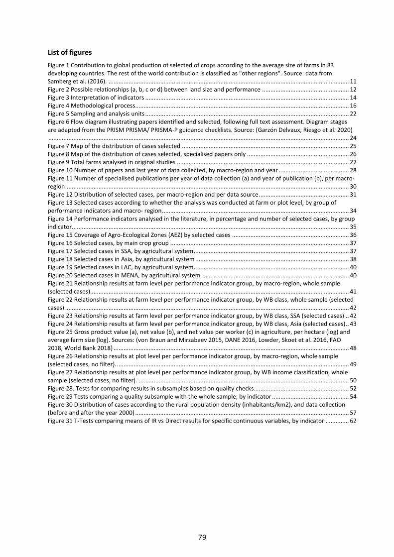
79

List of figures Figure 1 Contribution to global production of selected of crops according to the average size of farms in 83 developing countries. The rest of the world contribution is classified as "other regions". Source: data from Samberg et al. (2016). ................................................................................................................................................ 11 Figure 2 Possible relationships (a, b, c or d) between land size and performance .................................................... 12 Figure 3 Interpretation of indicators .......................................................................................................................... 14 Figure 4 Methodological process................................................................................................................................ 16 Figure 5 Sampling and analysis units .......................................................................................................................... 22 Figure 6 Flow diagram illustrating papers identified and selected, following full text assessment. Diagram stages are adapted from the PRISM PRISMA/ PRISMA-P guidance checklists. Source: (Garzón Delvaux, Riesgo et al. 2020) .................................................................................................................................................................................... 24 Figure 7 Map of the distribution of cases selected .................................................................................................... 25 Figure 8 Map of the distribution of cases selected, specialised papers only ............................................................. 26 Figure 9 Total farms analysed in original studies ....................................................................................................... 27 Figure 10 Number of papers and last year of data collected, by macro-region and year .......................................... 28 Figure 11 Number of specialised publications per year of data collection (a) and year of publication (b), per macro-region .......................................................................................................................................................................... 30 Figure 12 Distribution of selected cases, per macro-region and per data source ...................................................... 31 Figure 13 Selected cases according to whether the analysis was conducted at farm or plot level, by group of performance indicators and macro- region ................................................................................................................ 34 Figure 14 Performance indicators analysed in the literature, in percentage and number of selected cases, by group indicator ...................................................................................................................................................................... 35 Figure 15 Coverage of Agro-Ecological Zones (AEZ) by selected cases ...................................................................... 36 Figure 16 Selected cases, by main crop group ........................................................................................................... 37 Figure 17 Selected cases in SSA, by agricultural system ............................................................................................. 37 Figure 18 Selected cases in Asia, by agricultural system ............................................................................................ 38 Figure 19 Selected cases in LAC, by agricultural system ............................................................................................. 40 Figure 20 Selected cases in MENA, by agricultural system......................................................................................... 40 Figure 21 Relationship results at farm level per performance indicator group, by macro-region, whole sample (selected cases)........................................................................................................................................................... 41 Figure 22 Relationship results at farm level per performance indicator group, by WB class, whole sample (selected cases) .......................................................................................................................................................................... 42 Figure 23 Relationship results at farm level per performance indicator group, by WB class, SSA (selected cases) .. 42 Figure 24 Relationship results at farm level per performance indicator group, by WB class, Asia (selected cases) .. 43 Figure 25 Gross product value (a), net value (b), and net value per worker (c) in agriculture, per hectare (log) and average farm size (log). Sources: (von Braun and Mirzabaev 2015, DANE 2016, Lowder, Skoet et al. 2016, FAO 2018, World Bank 2018) ............................................................................................................................................. 48 Figure 26 Relationship results at plot level per performance indicator group, by macro-region, whole sample (selected cases, no filter). ........................................................................................................................................... 49 Figure 27 Relationship results at plot level per performance indicator group, by WB income classification, whole sample (selected cases, no filter). .............................................................................................................................. 50 Figure 28. Tests for comparing results in subsamples based on quality checks ......................................................... 52 Figure 29 Tests comparing a quality subsample with the whole sample, by indicator .............................................. 54 Figure 30 Distribution of cases according to the rural population density (inhabitants/km2), and data collection (before and after the year 2000) ................................................................................................................................ 57 Figure 31 T-Tests comparing means of IR vs Direct results for specific continuous variables, by indicator .............. 62

80

List of tables Table 1 Indicators to assess farm performance .......................................................................................................... 12 Table 2 Data sources ................................................................................................................................................... 17 Table 3 Inclusion and exclusion criteria ...................................................................................................................... 20 Table 4 Distribution of papers and case studies by macro-region ............................................................................. 25 Table 5 Distribution of papers and case studies by World Bank income classification .............................................. 26 Table 6 Distribution of farms included in collected papers and studies..................................................................... 27 Table 7 Ranking of publications with > 2 papers on the topic (294 papers)............................................................... 28 Table 8 List of most frequent publications with specialised papers (37 specialised papers) ..................................... 30 Table 9 Sample size of studies according to data source ........................................................................................... 31 Table 10 Summary statistics of land size of farms and plots, for selected cases per world macro-region, in hectares .................................................................................................................................................................................... 32 Table 11 Summary statistics of land size of farms and plots, for selected cases per WB Income per capita class, in hectares ...................................................................................................................................................................... 33 Table 12 Comparing the prevalence of IR estimations with respect to direct relationship between performance indicators, by macro- region and WB income class at farm-level, all sample, no filters. ........................................... 43 Table 13 Comparing the prevalence of IR estimations with respect to all other relationships between performance indicators, by macro- region and WB income class at farm-level, all sample, no filters ............................................ 44 Table 14 Comparing the prevalence of IR estimations with respect to direct relationship between performance indicators, by Agro-ecological zones (AEZ) at farm-level, all sample, no filters. ........................................................ 45 Table 15 Comparing the prevalence of IR estimations with respect to direct relationship between performance indicators, by main crop (FAO classification) at farm-level, all sample, no filters. ..................................................... 45 Table 16 Comparing the prevalence of IR estimations with respect to direct relationship between performance indicators, by farm system in SSA (Dixon et al. 2001) at farm-level, all sample, no filters. ....................................... 46 Table 17 Comparing the prevalence of IR estimations with respect to direct relationship between performance indicators, by farm system in ASIA, East-Asia and Pacific (Dixon et al. 2001) at farm-level, all sample, no filters. ... 46 Table 18 Comparing the prevalence of IR estimations with respect to direct relationship between performance indicators, by farm system in ASIA, South-East Asia (Dixon et al. 2001) at farm-level, all sample, no filters. ........... 47 Table 19 Comparing the prevalence of IR estimations with respect to direct relationship between performance indicators, by macro- region and WB income class at farm-level, all sample, no filters. ........................................... 51 Table 20 Comparing the prevalence of IR estimations with respect to all other relationships between performance indicators, by macro- region and WB income class at farm-level, all sample, no filters ............................................ 51 Table 21 Compared prevalence of IR estimation between performance indicator groups, according to selected sub-samples or quality filters, at farm level(). ................................................................................................................... 52 Table 22 Association of quality variables to IR vs. direct relationship*...................................................................... 54 Table 23 Comparing the prevalence of IR with respect to direct relationship between performance indicators, for all region, and by income class for SSA and Asia ........................................................................................................ 58 Table 24 Comparing the prevalence of IR with respect to direct relationship between performance indicators, for SSA, by income class for data before and after the year 2000. .................................................................................. 59 Table 25 Comparing the prevalence of IR with respect to direct relationship between performance indicators, for SSA, by income class for data before and after the year 2000. .................................................................................. 59 Table 26 Association of contextual variables to IR vs. direct relationship* ............................................................... 60 Table 27 Association of explanatory variables to IR vs. direct relationship* ............................................................. 61 Table 28 Association of explanatory variables to IR vs. direct relationship* ............................................................. 63 Table 29 FAOSTAT definitions ..................................................................................................................................... 77

GETTING IN TOUCH WITH THE EU

In person

All over the European Union there are hundreds of Europe Direct information centres. You can find the address of the centre nearest you at: https://europa.eu/european-union/contact_en

On the phone or by email

Europe Direct is a service that answers your questions about the European Union. You can contact this service:

- by freephone: 00 800 6 7 8 9 10 11 (certain operators may charge for these calls),

- at the following standard number: +32 22999696, or

- by electronic mail via: https://europa.eu/european-union/contact_en

FINDING INFORMATION ABOUT THE EU

Online

Information about the European Union in all the official languages of the EU is available on the Europa website at: https://europa.eu/european-union/index_en

EU publications You can download or order free and priced EU publications from EU Bookshop at: https://publications.europa.eu/en/publications. Multiple copies of free publications may be obtained by contacting Europe Direct or your local information centre (see https://europa.eu/european-union/contact_en).

XX-N

A-X

XXXX

-EN-N

KJ-N

A-30471-EN-N

doi:10.2760/140208

ISBN 978-92-76-26822-2