Policy Research Working Paper 5908

Fact or Artefact

The Impact of Measurement Errors on the Farm Size - Productivity Relationship

Calogero Carletto Sara SavastanoAlberto Zezza

The World BankDevelopment Research GroupPoverty and Inequality TeamDecember 2011

WPS5908P

ublic

Dis

clos

ure

Aut

horiz

edP

ublic

Dis

clos

ure

Aut

horiz

edP

ublic

Dis

clos

ure

Aut

horiz

edP

ublic

Dis

clos

ure

Aut

horiz

ed

Produced by the Research Support Team

Abstract

The Policy Research Working Paper Series disseminates the findings of work in progress to encourage the exchange of ideas about development issues. An objective of the series is to get the findings out quickly, even if the presentations are less than fully polished. The papers carry the names of the authors and should be cited accordingly. The findings, interpretations, and conclusions expressed in this paper are entirely those of the authors. They do not necessarily represent the views of the International Bank for Reconstruction and Development/World Bank and its affiliated organizations, or those of the Executive Directors of the World Bank or the governments they represent.

Policy Research Working Paper 5908

This paper revisits the role of land measurement error in the inverse farm size and productivity relationship. By making use of data from a nationally representative household survey from Uganda, in which self-reported land size information is complemented by plot measurements collected using Global Position System devices, the authors reject the hypothesis that the inverse relationship may just be a statistical artifact linked to problems with land measurement error. In particular, the

This paper is a product of the Poverty and Inequality Team, Development Research Group. It is part of a larger effort by the World Bank to provide open access to its research and make a contribution to development policy discussions around the world. Policy Research Working Papers are also posted on the Web at http://econ.worldbank.org. The author may be contacted at gcarletto@worldbank.org.

paper explores: (i) the determinants of the bias in land measurement, (ii) how this bias varies systematically with plot size and landholding, and (iii) the extent to which land measurement error affects the relative advantage of smallholders implied by the inverse relationship. The findings indicate that using an improved measure of land size strengthens the evidence in support of the existence of the inverse relationship.

1

Fact or Artefact: The Impact of Measurement Errors on

the Farm Size - Productivity Relationship1

Calogero Carletto2

Sara Savastano

Alberto Zezza

Keywords: Inverse Farm Size Productivity Relationship, Land Measurement Error, Uganda,

JEL Classification: O13, Q12, C81,

Corresponding Author:

Gero Carletto

The World Bank

1818 H St. NW

Washington DC, 20433

Email: gcarletto@worldbank.org

1 The views expressed in this paper are the authors‟ only and should not be attributed to the institutions they are

affiliated with. The authors are grateful to Hans Binswanger, Keijiro Otsuka, Franco Peracchi, Christopher Udry,

Paul Winters, and participants in the ICAS-V Conference in Kampala, Uganda (October 2010) for their

comments on an early version of this work. 2 Calogero Carletto and Alberto Zezza are with the Development Research Group of the World Bank. Sara

Savastano is with the University of Rome, Tor Vergata.

2

1. Introduction

The controversy over the existence of an inverse relationship between farm size and

productivity (IR henceforth) is one of the longest standing and more ideologically charged pieces of

the agricultural development literature. Should smallholders be found to be more efficient, policies to

facilitate the redistribution of land towards small famers may be justified not only on equity but also

on efficiency grounds. Binswanger et al. (1995) and Eastwood et al. (2010) provide comprehensive

reviews of the arguments and a historical account of the empirical evidence on the IR. In the context

of African agriculture, the relationship has been most recently questioned by Collier and Dercon

(2009) who maintain that “there are (only) a handful of reasonably careful studies showing the inverse

farm-size/productivity relationship in African settings, but also some showing the reverse (i.e.

positive) farm-size/productivity relationship”.

A substantial part of the debate, particularly in recent years, has focused on whether the IR

may be a statistical artifact, stemming from problems with the available data. The possible role of the

omission or imprecise measurement of land quality traits in determining the empirical findings on the

IR has been examined by several authors (Walker and Ryan, 1990; Binswanger et al., 1995; Benjamin,

1995; Bhalla and Roy, 1998; Lamb, 2003). Barrett et al. (2010) have probably put an end to that aspect

of the controversy convincingly using laboratory tests on soil samples to show that only a minimal part

of the IR can be explained by differences in land quality. We are aware of only one study (Lamb,

2003) that attempts to empirically test the robustness of the IR to possible errors in land area

measurement. The conclusion of that study, which controls for errors in land measures indirectly by

comparing fixed and random effect estimates, is that when errors in self-reported farm size are

accounted for the IR can be completely explained by factor market imperfections and differences in

land quality.

In this paper, we revisit the role of land measurement error in the IR controversy by drawing

on data from a nationally representative household survey from Uganda, in which self-reported land

size information were complemented by plot measurements collected using Global Position System

(GPS) devices. This allows us to systematically analyze the differences in land area data using both

measurements, and discuss the impact of such differences on estimates of agricultural productivity. In

particular, we explore: (i) what are the determinants of the bias in land measurement, (ii) whether this

bias varies systematically with plot size and landholding, and (iii) whether the data support the IR

hypothesis, and the extent to which land measurement error affects the relative advantage of

smallholders implied by the IR. Preliminary empirical evidence (Goldstein and Udry, 1999) suggests

that the differences between GPS and self-reporting may be substantial, and that such difference varies

by farm size. If this intuition is correct, using GPS data can have considerable implications for the

much debated and contentious relationship between farm size and productivity.

3

The paper is organized as follows. The next section succinctly reviews the main strands of

literature this paper relates to. Section 3 provides a description of the data. The econometric models

used are sketched in Section 4 and the results discussed in Section 5. The final section summarizes the

contributions of the analysis to the literature and to the policy discussion around smallholders‟

productivity.

2. The inverse farm size-productivity relationship: Smallholder advantage or statistical

artefact?

Starting with the seminal work of Sen (1962, 1966) who observed an inverse relationship

between farm size and output per hectare in Indian agriculture, a large number of empirical studies

have presented evidence that appears to corroborate that hypothesis (Barrett, 1996; Carter, 1984,

Eswaran and Kotwal, 1985, 1986; Lau and Yotopoulos, 1971; Benjamin and Brandt, 2002; Berry and

Cline, 1979). A smaller set of empirical studies however does not find evidence of such a relationship

(Hill, 1972, Kevane, 1996, Zaibet and Dunn, 1998). Binswanger et al. (1995) and Eastwood et al.

(2010) provide careful discussions of both the theory and the empirics of the IR debate, a full review

of which is beyond the scope of this paper.

It will suffice here to note that, following Barrett et al. (2010), an inverse relation between

farm size and productivity may have three main explanations: (i) imperfect factor markets, (ii)

omitted variables and, in particular, omitted controls for land quality, and (iii) statistical issues related

to the measurement of plot size. Imperfect factor markets (labor, land, insurance) are linked to

differences in the shadow price of production factors that in turn lead to differences in the application

of inputs per unit of land, in ways that are correlated with farm size. Much of the earlier contributions

to the IR debate focused on testing this type of explanation. Assunçao and Ghatak (2003) demonstrate

how theoretically unobserved heterogeneity in farmer quality may explain the observed differences in

productivity. Other studies (e.g. Bhalla and Roy, 1988; Benjamin, 1995) have challenged the existence

of the IR based on the observation that when land quality controls are introduced in the analysis, the

strength of the IR often diminishes substantially or vanishes altogether. Barrett et al. (2010) utilize a

dataset that includes laboratory measures of soil testing to conclude that in fact only a very limited

proportion of the IR can be explained by differences in land quality. Lastly, attention has been drawn

to the possibility that the existence of the IR may be a statistical artifact deriving by measurement

error in land data (Lamb, 2003). A similar explanation is also hinted at by Barrett et al. (2010), after

failing to explain the observed IR otherwise.

For the IR to be partially or fully explained by errors in land measurements, smaller farmers

would have to systematically underreport land area with respect to larger farmers, thus resulting in

artificially inflated yields in the bottom part of the distribution. However, as reported by De Groote

4

and Traorè (2005), small farmers tend to overestimate their land holding – while large farmers tend to

underreport – hence increasing the likelihood of analysts finding an even stronger inverse relationship

in empirical studies based on more accurate measures.

Land area measurement is one of the fundamental components of agricultural statistics, and it

is therefore not surprising that the interest of agricultural statisticians in the possibility of applying

technological innovations such as satellite imagery and GPS devices to land area measurement is

growing exponentially with the increasing affordability and precision of these technologies and their

applications. Kelly et al. (1995) have long identified the use of GPS has having the potential to

contribute to making land area measurement a much less costly and time consuming exercise than

traditional methods. An early study mentioning a comparison of GPS and self-report plot measures is

Goldstein and Udry (1999). They only refer to this in passing in a study of agrarian innovation in the

Eastern Region of Ghana, reporting a very low correlation coefficient of just 0.15 between the two

measures. They explain the result with the fact that traditional land measures in the region were based

on length only (ropes), and as land became more scarce local farmers found it difficult to translate that

to a two dimensional measure (hectares).

Keita and Carfagna (2009) provide a discussion of the performance of different GPS devices

compared to traditional methods (rope and compass), which they consider the „gold standard‟. Their

evidence confirms that GPS devices allow measuring farm size with enough accuracy compared to

traditional and objective land measurement methods such as compass and meters. They conclude that

the GPS is a reliable alternative to traditional measures (80 percent of the plots in their sample is

measured with negligible error), but that on average GPS measures tend to underestimate plot area

somewhat. The main reasons for errors in GPS measures detected by this study are the density of plot

tree canopy cover and to some degree weather conditions at the time of measurement.

In a somewhat different application in the context of Peruvian market access self-reported data

vis a vis “true travel time” using GPS, Escobal and Laszlo (2008) show how if the error is correlated

with the main outcomes of interest the conclusions of the analysis may be biased and driven by a

spurious correlation. That is because the deviation between the „true‟ travel time and the respondents‟

estimate is determined by observable socio-economic variables related to the outcome of choice.

Gibson and Mckenzie (2007) show evidence of the non-random distribution of measurement error in

several of the distance and location studies they review, and demonstrate how the use of GPS aids can

help overcome problems of measurement in data collection efforts.

GPS measurements are of course not immune from problems themselves. Possibly the most

important issue is the fact that it is generally not practical and too costly to measure all the plots

owned by a household. Some plots may be distant from the place of the interview (usually the

household‟s dwelling), and respondents may not have the time or be willing to accompany the

5

enumerators to all the plots. Even if they were, the operational costs and travel time required to record

GPS measures for all plots are likely to be prohibitive for most survey operations. This raises some

analytical concerns, in the form of biased estimates, if the plots that are not measured are

systematically different from the ones that are measured. We do find evidence of such bias in our data,

and in the next section we discuss how we dealt with the issue.

3. Data source and descriptive statistics

The data for this paper come from the Uganda National Household Survey (UNHS) round

implemented by the Uganda Bureau of Statistics (UBOS) in 2005-2006. The UNHS is a multi-purpose

household survey with a sample of 7,500 households, selected following a stratified sample design that

identified 753 enumeration areas (UBOS, 2009). One special feature of this survey that makes our

analysis possible is that it contains plot level information on agricultural land area measured through

both GPS and farmers‟ own estimates.

Some 5, 714 of the survey households are located in rural areas and cultivate land. The total

number of plots with self-estimated measure is 13,959 and about 65 percent of these (9,173 plots) have

a corresponding GPS measure3. The agricultural production section, however, only contains

information gathered at the household/farm level. Thus, the analysis in this paper is carried out partly

at the plot level, and partly at the household/farm level. We use the former to analyze the difference

between land area measurement using farmers‟ estimate and GPS, since it is at the plot level that the

two measures are collected. The household/farm level analysis is more suitable to investigate the

consequences of the bias in land measurement on the IR, since key farm input and output data are only

available in the survey at this level, not allowing the calculation of plot-specific productivity measures.

To be able to run the analysis maintaining a consistent sample throughout, we therefore

restricted our sample further to 5,767 plots for which we have complete information on both type of

measures for all the plots cultivated by the household. In the farm level analysis, for which we also

drop 42 households with negative farm profits (equivalent to 1.5 percent of the sample), we end up

with a sample of 2,860 rural households for which we have both non-zero land area measures for the

entire households‟ landholdings.

Table 1 reports key summary statistics for the plots for which we have information on both

types of area measurements, along with the mean and standard deviation (in acres) of plot size

measured through GPS, self-reporting, and the absolute and relative difference between the two

measures. For simplicity of presentation, we will take the GPS measure as the benchmark and talk of

farmers over- (or under-) reporting plot size whenever the area self-reported is larger (smaller) than

the area measured by GPS. We do acknowledge however that the GPS measure may also be subject to

a certain degree of inaccuracy (Keita and Carfagna, 2009).

3 A Garmin 12XL GPS device was used by the survey teams to collect plot area data.

6

On average the two methods produce strikingly similar estimates of land area. The average

size of plots using GPS is 2.24 acres, a mere 0.11 acres (equivalent to 4.9%) larger than the area

reported by farmers. The sample level means however mask pervasive differences in measurement that

emerge at closer scrutiny. In the overall sample, farmers overestimate plot size in 54.12 percent of the

cases (or 3,121 plots), and underestimate it in 44.13 percent of plots (equivalent to 2,545 plots). For

the remaining 101 plots (1.75 percent) the survey reports identical measures with either method. For

the plots where a „positive discrepancy‟ is observed, namely a GPS measure larger than self-reporting,

the amount of area overestimated is larger in absolute value (1.07 acres on average, or 35.1 percent)

than for the plots for which the bias is negative (-0.67 acres or 47.2 percent).

The fact that we dropped a substantial number of plots from our analysis because of gaps in

the GPS measurement raises some concerns regarding whether this may introduce a source of bias in

our analysis. This intuition is partially confirmed by an inspection of the summary statistics for the

two sets of plots. Annex Table 1 reports the means and t-tests for the difference in means for some key

plot and household characteristics. The plots that we had to exclude from the analysis because of gaps

in the GPS measure are on average smaller than those we did include, they are more likely to be on a

steep slope, and less likely to be protected by a fence. The heads of households to which these plots

belong are somewhat older and less educated, and more likely to be female. Also, these plots belong to

households that are on average smaller. These plots are therefore not randomly selected, which is what

one would expect, since taking the actual GPS measurement of a plot requires a household member

and enumerator to move for the site of the main interview to the location of the plot to take the GPS

measurement. More distant, less accessible plots are therefore more likely to be excluded. These

statistically significant differences in plot characteristics between the part of the sample we use and the

part we had to discard suggest the presence of possible sample selection issues arising from these

restrictions and impacting on the analysis of farm productivity. We will return to this point in the

result section, to show how these issues to do not in fact appear to be affecting our results. The non-

random selection of GPS-measured plots, however, does represent a challenge that future surveys

employing these methodologies will have to find ways to confront.

Table 2 summarizes land measurement statistics at the household level. We report statistics for

deciles of landholding to investigate how measurement bias plays out at different points of the

distribution. This information will be important later, when we analyze the impact of land

measurement bias on the IR. The last column of table 2 reports the discrepancy in percentage terms.

According to this measure, the magnitude of the discrepancy appears to increase monotonically as one

moves from the bottom (smallest landholders, -97 percent) to the top deciles (largest landholders, 19

percent). Up to 4.57 acres of farm size (the seventh decile), the bias is on average negative, whereas it

becomes positive in the top three deciles. There is therefore a pattern in the direction of the bias, with

7

smaller farmers generally over reporting their land relatively more than larger farmers, and with the

largest farmers actually under reporting land size.

These findings go in the same direction as the results of De Groote and Traorè (2005) for

Southern Mali. As stated above, De Groote and Traorè find that there is an approximate linear

negative relationship between measurement error and plot size. Farmers have a tendency to

overestimate small plots (which they define as below 1 hectare4) compared to larger ones, which they

somewhat underestimate. Also, the GPS and self-reported plot area measures in our sample display a

correlation of 0.97 (which drops to a more reasonable, but still respectable, 0.77 when we trim the

right end of the distribution of a few very large plots), well above the 0.15 found by Goldstein and

Udry (1999) in their Ghana dataset.

One additional issue in our data, that is immediately apparent from the visual inspection of the

distributions of the two land measures in Figure 1, is the considerable tendency of respondents (or

enumerators) to round their reported plot size to nearest acre or half acre. This „heaping‟ in the

response pattern is not uncommon (Roberts and Brewer, 2001) but we suspect it may be particularly

important in the case of land measurement since it is bound to matter proportionally more to the left

of the distribution, as the same amount of rounding represents a larger percentage of the actual plot

size.

Figure 1 also confirms that the two distributions are, overall, quite similar. However, while

the means are not much different, at specific points the distributions deviate considerably, in a way

that appears to be driven by heaping in the self-reporting distribution as opposed to a smooth curve for

the GPS measure. Finally, the comparison of the two distributions appears to support the case for

treating the GPS measure as the more accurate of the two.

The systematic patterns in the difference between land measurements we have observed above

have the potential to introduce a bias in the estimation of agricultural/land productivity. Reasoning

through the data it is apparent, as we already mentioned, that the kind of pattern we observe in our

data should, if anything, generate a bias opposite in sign to that needed to corroborate the IR

hypothesis. If small farmers report to be cultivating more land than they actually are, their „true‟ yields

are actually even larger than what one would compute using self-reported land quantities. To explore

that point descriptively, Figure 2 draws the relationship between deciles of cultivated land and farm

yields (computed as the ratio of the value of agricultural production over farm size). The slope of both

lines is negative, pointing to an inverse yield-farm size relationship in both cases, but the line is even

steeper when the GPS land measure is used.

Table 3 summarizes farm yields computed using GPS and self-reported land areas. Farms are

categorized as small, medium or large. Small farms, those cultivating landholdings smaller than1.45

4 1 hectare is equal to 2.47 acres.

8

acres exhibit systematically higher yields when area cultivated is measured through GPS as compared

to self-reporting. The distance is reduced for medium farms, whereas large farms have lower yields

measured with GPS than those obtained through farmers estimate.

The inclusion of a more accurate measure of land area in this dataset seems to be

strengthening the empirical case for the existence of an inverse farm size productivity relationship,

rather than weakening it. This is consistent with what we expected after looking at the distribution of

the discrepancies in the two measures, but appears to contradict the discussion in Barrett et al. (2010)

and the analysis in Lamb (2003), who finds that the IR disappears after introducing random effects

which he hypothesizes capture the influence of measurement error.

4. The econometric approach

In order to deepen the analysis of (a) the characteristics and determinants of the discrepancy

between our two land measures, and (b) the implications of measurement bias on the robustness of the

IR hypothesis, we estimate the two models specified below.

As in Deininger et al. (2011), to identify what are the factors affecting the difference between

the two measures we estimate the following function, at the plot level:

jjjuxe (1)

Where j

e is the plot size specific difference between the GPS and the self-reported measure,

jx is a (K+1)-row vector of control variables with „1‟ as its first element,

)',...,,(10 K

is

vector of parameters to be estimated. j

u is a two-sided error term representing white noise The

controls used in this regression include a set of characteristics of the household head (age, education,

and gender) to proxy respondents‟ characteristics that are deemed to influence the ability to accurately

report land size. We also include plot size, and its squared term, to test whether the relationship

observed in the descriptive analysis holds in a multivariate framework, and a dummy reflecting

whether the self-reported land variable is a round number, to capture the impact of rounding. We

include information on whether the household is involved in disputes over land ownership, as we

expect such households to have less information or interest in these plots. Topography will also affect

land estimate by farmers, as steep plots may be more likely to be subject to measurement error.

Finally, we also add PSU dummies to control for idiosyncratic differences across survey teams and

supervisors and for possible environmental and geographic factors.

Next we estimate a standard model for testing the existence of the IR, and to understand how

land measurement error weakens, eliminates or reinforces this empirical evidence. Our model is based

9

on the one originally proposed by Binswanger, Deininger and Feder (1995), and not dissimilar from

the approach used by several others including, most recently, Barrett et al. (2010). We estimate the

following function at the household level:

iii

i

iuRXA

A

Y

3210lnln (2)

where iY

represents net agricultural revenues for each household i, iA

the total area operated,

iX

denotes a vector of households‟ characteristics that influence production such as the availability of

family labor, the gender, age and education of the household head, value of inputs used, and a set of

land quality variables, R is the rounding effect when net revenues per acre of area cultivated are

measured with land size as reported by farmers, and iu

is the error term. We estimate two versions of

this relationship, one using GPS and the other one with the self-reported land measure, and compare

the two to gauge the impact of differences in measurement on the IR, which is captured by the

coefficient on the land size variable. A negative coefficient on the land area variable indicates the

presence of the IR. The further below 0 the coefficient, the stronger the IR. As in the previous model,

we also include PSU fixed effects to control for survey team and local environmental effects.

The left hand side term - net agriculture revenues per acre - is computed as the value of total

crop production net of value of variable inputs (hired labor, seeds, organic and inorganic fertilizers,

chemicals, and animals rented for plowing), divided by the amount of land cultivated. While we

maintain this is the preferred way to calculate net revenues, some may argue that subtracting hired but

not family labor may give an unfair advantage to small farmers who rely mainly on the latter. We

therefore also tried running our estimates without subtracting hired labor costs from gross revenues

and the results (not reported) did not change to any significant extent.

Regarding the terms on the right hand side, we expect productivity to be positively related to

the use of variable farm inputs, including hired labor. Given the supportive evidence provided by

several of the contributions to the inverse farm size productivity debate (Lau and Yotopoulos 1971;

Berry and Cline 1979; Kutcher and Scandizzo 1981; Carter 1984; Eswaran and Kotwal 1985; 1986;

Barrett 1996; Udry 1996; Benjamin and Brandt 2002), we expect labor market imperfections to give

an advantage to farms able to rely on family labor, and hence a positive sign on the coefficient on this

variable.

To control for various aspects of land quality, variables on farmer-assessed soil quality,

steepness and irrigation of the plots are included as regressors. The soil quality variable is computed

as the share of total cultivated land the farmer reports being in plots with good soil quality. The share

of steep land is similarly computed using plot level data, and taking the sum of plot size with steep

slope as a share of the total landholding. In the same fashion the share of land irrigated is constructed

10

dividing the area of the cultivated plots reported to be irrigated by the total cultivated acreage. The

obvious expectations concerning the regression coefficients on these variables are that good quality,

irrigated land will be associated with larger profits per acre, whereas greater shares of steep land will,

other things equal, be associated with lower levels of productivity per unit of cultivated land.

The final set of variables in the regression relates to household characteristics. The age of the

household head is normally expected to reflect farming experience and therefore be positively related

to farm productivity. It is also possible that older age may be related to reduced physical strength,

health problems and hence reduced ability to farm the land, but the experience aspect usually

dominates. Education should clearly affect positively farmers‟ productivity and welfare, while the

expectation is for female headed households to be less productive because of a wide variety of factors

ranging from discrimination in input and output markets to unfavorable family composition. Where

the female headship is due to the presence of a migrating husband sending remittances back home that

can be invested in farming, however, the impact on farming and productivity may in fact be positive.

5. Empirical results

The results of the estimation of model (1) are reported in Table 4. Confirming the results of

the descriptive analysis in section 3, the data show a positive association between plot size and the

difference between GPS and self-reported land measurements in levels. This discrepancy increases

with farm size: larger farms have a tendency to under-report, while small farms tend to over-state the

size of their landholdings.

The other signs are also as expected. The presence of rounding contributes to increasing

measurement error, as we hypothesized based on the heaping displayed by the distribution of self-

reported plot size in Figure 2. While the education and gender of the household head variables are not

significant, head‟s age matters. Older heads are likely to be less accurate in their reporting of plot size.

Households who are involved in disputes over land are also likely to make larger errors in self-

reporting, which we hypothesize is due to the fact that such disputes diminish their interest, access,

and in general knowledge of plot characteristics. Contrary to expectations the demarcation of the plot

with a fence does not seem to reduce the error in land self-reporting; the coefficient of the dummy if

the plot has a fence is positive and significant thereby suggesting a larger error for those plots. Finally,

the steepness of the plot does not appear to significantly influence measurement bias.

Table 5 presents the results of the net revenue regression in model (2). In column (1) land is

measured with the traditional respondent self-report, whereas column (2) is based on the GPS measure

of land size. The main variable of interest in this model is the (log) of land size, as it is this coefficient

that captures the size-productivity relationship, with a negative coefficient pointing to the existence of

an inverse relationship. The estimated coefficients are -0.62 in the specification using self-reported

11

land size and -0.83 in the specification using the GPS measure of agricultural plots. Both estimates

therefore support the IR hypothesis. When the GPS measure of farm size is used, however, the

absolute value of the coefficient increases, indicating an even stronger IR.

The inclusion of hired labor and inputs on the right hand side poses problems as they may

capture part of the effect of market imperfections, not allowing for their full effect to be reflected in

the farm size coefficient5. To check for the extent to which this problem might affect our results we

run the same regression without these variables and the key results (not reported) did not change. In

both specifications, the coefficient of land size decreases of 0.1 but remains negative and statistically

significant.

The hypothesis according to which the IR would be a statistical artifact due to small farmers

under-reporting their farm size is therefore strongly rejected by the data. In our sample, small farmers

in fact over-report land size, and it is the very large famers who are actually more likely to under-

estimate their holdings, thus resulting in artificially higher yields. When more accurate land measures

are used thanks to the introduction of GPS devices, the estimated slope of the function becomes

steeper indicating an even stronger IR than what one would conclude based on similar estimates

performed using farmers‟ self-reporting.

As expected, good soil quality shows a positive association with farms profits, which remains

stable across specifications. The irrigation and steepness variables, on the other hand, have the

expected signs (positive for irrigation, negative for steep land) but the estimated coefficients are not

statistically significant.

As discussed in Section 3 above, one issue with our data is the sample selection bias

introduced by dropping from the productivity analysis the households for which we do not have both

measures for all plots. To investigate whether this may be a factor invalidating our main findings we

re-estimated model (2) using the entire sample, and tested (a) whether the group means of predictors

estimated using the two samples are equal, and (b) whether the main coefficients of interest for the IR

(i.e. the coefficients on the land variable) are equal. Results are reported in Annex Table 2.

The Wald test rejects the null hypothesis that all coefficients are equal for both samples, which

one would expect given the systematic differences between the two samples we reported in Annex

Table 1, and discussed earlier in the paper. What matters for our key results, however, is that the test

fails to reject the null for the land coefficient. In other words, the IR estimated using the self-reported

measure is as strong on the full sample as it is on the restricted sample for which we have complete

GPS information. For productivity analysis at large, however, the rejection of the test of equality

between the two runs of the model does point towards the need for future surveys to solve the

5 The input variables also pose possible endogeneity problems being choice variables for the farmers.

12

selection issues related to GPS measurement of plots, as that is bound to matter for specific aspects of

the analysis.

One final concern relates to the possibility that larger farms be concentrated in remote and

unfavorable agricultural areas, or that market imperfections leading to the IR may be confined to

particular regions. We investigated whether that appears to be the case in our data, by running our

analysis separately for the four macro-regions for which the UNHS is statistically representative

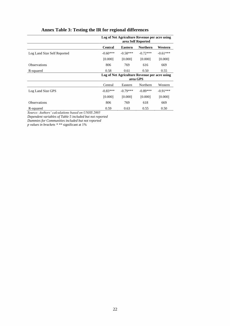
(Central, Eastern, Northern and Western Uganda). Annex Table 3 presents a summary of the analysis.

For brevity we only report the coefficient of land size, which is our variable of interest. The

specification is the same as that described in model (2) and reported in Table 5 for the full sample,

with the same explanatory variables included but not reported. The top panel of Annex Table 3 reports

the results of the IR between net revenue of crop production per acre computed using the self-reported

land area variable, for each of the 4 regions. The bottom panel shows the corresponding statistics for

the specification that uses the GPS area measurement. As in Table 5, we note that in all regions the IR

holds regardless of the specification, but that it is stronger when the GPS area measured is used. Our

results do not therefore appear to be sensitive to the effect of possible socio-economic or agro-

ecological differences across regions.

6. Conclusions

The hypothesis that the inverse relationship between farm size and productivity may just be a

statistical artifact, linked to problems with land measurement error, is rejected by the analysis

presented in this paper. Contrary to earlier conjectures, we find that the empirical validity of the IR

hypothesis is strengthened, not weakened, by the availability of better measures of land size collected

using GPS devices. Lamb (2003) concludes that by controlling for measurement error in land size, the

statistical case for the IR disappears. This paper has shown that introducing rigorous controls for land

quantity does not affect the evidence concerning the IR, which is in fact strengthened when the better

land data are used.

We also explored how farmers‟ self-reporting of plot size varies systematically with the size

of their holdings and other household and land characteristics. We conclude that in Uganda small

farmers tend to over-report plot size relative to medium-sized land-holders, while the largest farm

groups under-report plot size on average. This is consistent with earlier evidence from Mali reported

by De Groote and Traorè (2005).

Self-reported measures of land size are notoriously imprecise. In large household surveys in

developing countries, however, they have for a long time been the only option available to practically

collect data on the physical dimension of the plots owned or cultivated by the household. More

13

recently the availability of affordable and more reliable GPS devices has made GPS measurement a

practical alternative that is increasingly being applied in surveys worldwide.

Being able to measure land with any degree of accuracy is clearly of outmost importance in

economies that are largely agricultural based and for communities that derive a large share of their

livelihood from agriculture and for whom land constitutes the main, when not the only, capital asset.

In particular, an accurate measure of land size is necessary if one is to measure agricultural

productivity with any degree of confidence.

This paper has shown that GPS technologies clearly hold promise for improving the accuracy

in the collection of land size measures in the context of large household surveys. On the other hand,

while we are not able to account in full for the determinants of the deviation between GPS and self-

reported measures, we do find that self-reported land measures are a reasonable alternative in a well

conducted survey, particularly for medium-sized farmers. The overall distribution as well as their

mean and standard deviation, are fairly close to each other, and the measurement error did not change

the substance of our productivity analysis. The respondents‟ rounding of responses can however create

fairly serious differences in measurements, particularly when plots are small, as is the case here (but

also in most of the developing regions).

The continuing fall in the price and increasing precisions and reliability of GPS devices make

them an increasingly attractive element of every survey team toolbox. For mainly logistic reasons,

however, GPS readings are hardly ever taken on all plots, and this raises concerns on the potential

selectivity bias resulting from measuring only a sub-set of plots. While allocating adequate resources

could go a long way in ensuring that this bias is reduced, farmer‟s self-reported measures must also be

collected possibly together with information on the possible sources of the bias, to complement the

GPS estimates and correct for potential biases. How to do that in practice is a subject that warrants

further investigation.

14

References

Assuncao, J., Ghatak, M., 2003. On the Inverse Relationship between Farm Size and Productivity. Economics

Letters , Volume 80, No. 2, pp.189-194, August 2003

Barrett, C. B., 1996. On Price Risk and the Inverse Farm Size–Productivity Relationship. Journal of

Development Economics, 51(2), 193–215.

Barrett. C., Bellemare, M.F., Hou, J.Y., 2010. Reconsidering Conventional Explanations of the Inverse

Productivity–Size Relationship. World Development Vol. 38, No. 1, pp. 88–97, 2010

Benjamin, D., 1995. Can Unobserved Land Quality Explain The Inverse Productivity Relationship? Journal of

Development Economics 46 (February) :51-84 .

Benjamin, D., Brandt, L., 2002. Property Rights, Labor Markets, and Efficiency in a Transition Economy: The

Case Of Rural China. Canadian Journal of Economics, 35(4), 689–716.

Berry, R. A., Cline, W. R., 1979. Agrarian Structure and Productivity in Developing Countries. Baltimore: Johns

Hopkins University Press.

Bhalla, S. S., Roy, P., 1988. Mis-Specification in Farm Productivity Analysis: The role of land quality. Oxford

Economic Papers, 40, 55–73.

Binswanger, H. P., Deininger, K., Feder, G., 1995. “Power Distortions Revolt and Reform in Agricultural Land

Relations.” In J. Behrman and T.N. Srinivasan, eds., Handbook of Development Economics, Volume III.

Amsterdam, The Netherlands: Elsevier Science B.V.

Bound, J., Brown, C., Mathiowetz, N., 2001. Measurement Error in Survey Data, in J. Heckman and E. Leamer,

eds, Handbook of Econometrics, Vol. 5.

Carter, M. R., 1984. Identification of the Inverse Relationship Between Farm Size and Productivity: an

Empirical Analysis of Peasant Agricultural Production. Oxford Economic Papers, 36, 131–145.

Collier, P., Dercon S., 2009. African Agriculture In 50 Years: Smallholders in a Rapidly Changing World? Paper

presented at the Expert Meeting on How to Feed the World in 2050 Food and Agriculture Organization of

the United Nations Economic and Social Development Department, Rome, June 24-26.

Deininger, K., Carletto,G, Savastano S., Muwonge, J., 2011, Can Diaries Help Improving Crop Production

Statistics? Evidence from Uganda, Journal of Development Economics, forthcoming

De Groote, H., Traoré O., 2005. The Cost of Accuracy in Crop Area Estimation. Agricultural Systems 84:21-38

Escobal, J., Laszlo, S., 2008. Measurement Error in Access to Markets. Oxford Bulletin of Economics and

Statistics Volume 70(2), 209–243, April

Eswaran, M., Kotwal, A., 1985. A Theory of Contractual Structure in Agriculture, American Economic Review

75: 352-67.

Eswaran, M., Kotwal, A., 1986. Access to Capital and Agrarian Production Organization, Economic Journal 96:

482-98.

Gibson, J., McKenzie, D., 2007. Using the Global Positioning System in Household Surveys for Better

Economics and Better Policy. Policy Research Working Paper Series 4195, The World Bank.

Goldstein, M., Udry C., 1999. Agricultural Innovation and Risk Management in Ghana. Unpublished, Final

report to IFPRI.

Hill, P., 1972. Rural Hausa: a Village and a Setting. Cambridge: Cambridge University Press.

Keita N., Carfagna, E., 2009. Use of Modern Geo-Positioning Devices in Agricultural Censuses and Surveys,

Bulletin of the International Statistical Institute, the 57th Session, 2009, Proceedings, Special Topics

Contributed Paper Meetings (STCPM22), Durban, August 16-22.

Kelly, V., B. Diagana, T. Reardon, M. Gaye, Crawford, E., 1995. Cash Crop and Foodgrain Productivity in

Senegal: Historical View, New Survey Evidence, and Policy Implications. MSU Staff Paper No. 95-05. East

Lansing: Michigan State University

Kutcher, G. P., Scandizzo, P.L., 1981. The Agricultural Economy of Northeast Brazil. The Johns Hopkins

University Press.

15

Kevane, M., 1996. Agrarian Structure and Agricultural Practice. Typology and Application to Western Sudan.

American Journal of Agricultural Economics, 78(1), 236–245.

Lamb, R. L., 2003. Inverse Productivity: Land Quality, Labor Markets, and Measurement Error. Journal of

Development Economics, 71(1), 71–95.

Lau, L. J., Yotopoulos, P.A., 1971. A Test for Relative Efficiency and Application to Indian Agriculture.

American Economic Review 61: 92-109.

Roberts, John M. , Brewer, Devon D., 2001. Measures and Tests of Heaping in Discrete Quantitative

Distributions. Journal of Applied Statistics. 28(7):887-896.

Sen, A. K., 1962. An Aspect of Indian Agriculture. Economic Weekly, 14, 243–266.

Sen, A. K., 1966. Peasants and Dualism with or Without Surplus Labor. Journal of Political Economy, 74(5),

425–450.

UBOS, 2009. Uganda National Household Survey 2005/2006, Study Documentation.

Walker, T.S., Ryan, J.G., 1990. Village and Household Economies in India's Semi-arid Tropics. , Johns Hopkins

Univ. Press, Baltimore.

Zaibet, L. T.;. Dunn E.G. 1998. Land Tenure, Farm Size, and Rural Market Participation in Developing

Countries: The Case of the Tunisian Olive Sector. Economic Development and Cultural Change, Vol. 46.

16

TABLES

Table 1: Summary of statistics at the plot level

Nb of Plots Unit Mean Std. Dev. Min Max

GPS 5767 Acre 2.24 12.43 0.01 600

Self – Reported 5767 Acre 2.13 12.75 0.01 600

Discrepancy (GPS-Self reported) 5767 Acre 0.11 2.28 -49 45

Negative discrepancy

(Negative Error => GPS<Self Reported ) 3121 Acre -0.67 1.82 -49 -0.01

Positive discrepancy

(Positive Error => GPS>Self Reported) 2545 Acre 1.07 2.47 0.01 45

Source: Authors’ calculations based on UNHS 2005

Table 2: Mean farm size and discrepancy characteristics by decile of landholding (GPS

measure)

Deciles Area of

HH landholding

Nb. of

plots per

hh

Mean

farm area

using

GPS

Mean

farm area

using

Self-Reported

Farm Discrepancy

(GPS-Self Reported)

Discrepancy in %

terms

1 0.01-.65 1.70 0.37 0.73 -0.36 -97%

2 0.66-1.12 2.33 0.90 1.43 -0.53 -59%

3 1.13-1.62 2.40 1.37 1.78 -0.41 -30%

4 1.63-2.09 2.70 1.84 2.36 -0.52 -28%

5 2.09-2.69 2.94 2.38 2.91 -0.52 -22%

6 2.7 2.80 3.04 3.53 -0.48 -16%

7 3.44-4.57 2.74 3.96 4.10 -0.14 -4%

8 4.59-6.16 2.94 5.31 5.18 0.13 2%

9 6.17-9.13 3.20 7.46 7.08 0.39 5%

10 9.14-600 3.40 21.03 17.07 3.96 19%

Total 0.01-600 2.70 4.75 4.60 0.15 3%

Note: area is expressed in acres, and computed for total household landholding.

Source: Authors’ calculations based on UNHS 2005

17

Table 3: Relation between yields and farm size

Landholding

Average

land

area

Yields

(GPS)

Yields

(Self Reported)

Bias in yields

(GPS-Self Reported)

Acres Acres US$/acre US$/acre %

Small Farms 0.01-1.45 0.7 236 170 28%

Medium Farms 1.46-3.57 2.4 208 193 7%

Large Farms 3.58- 600 10.3 77 100 -30%

Source: Authors’ calculations based on UNHS 2005

Table 4: Determinants of difference in plot measurement (dependent variable: GPS-self

reported plot size, in acres)

Bias in Level

With PSU

Fixed Effects

Plot size (GPS)

0.04***

[0.000]

Plot size (GPS) squared -0.001***

[0.000]

Rounding in Self Reported 0.26***

[0.001]

Dummy: parcel has a fence 0.45***

[0.006]

Head's age 0.73***

[0.000]

Head‟s Education -0.01

[0.566]

Dummy: Female household head 0.07

[0.362]

Dummy: Plot was/is in dispute with relatives 0.67***

[0.004]

Dummy: Plot is steep 0.20

[0.349]

Constant -0.55***

[0.000]

Observations 5,767

R-squared 0.229

Source: Authors’ calculations based on UNHS 2005

p values in brackets

* significant at 10%; ** significant at 5%; *** significant at 1%

18

Table 5: Testing the IR hypothesis. Dependent variable log of net agriculture revenue

per acre (with robust standard error)

Area Self-

Reported Area GPS

(1) (2)

Log Land Size -0.62*** -0.83***

[0.000] [0.000]

Dummy: Rounding 0.01

[0.893]

Log value of ag. Inputs 0.10*** 0.08***

[0.000] [0.000]

Log family labor 0.49*** 0.42***

[0.000] [0.000]

Log hired labor 0.02 0.03

[0.218] [0.115]

Share of land with good 0.18*** 0.23***

soil quality [0.001] [0.000]

Share of land steep -0.22 -0.01

[0.217] [0.959]

Share of land irrigated 0.33 0.07

[0.145] [0.766]

Log Head's age 0.001 0.001

[0.373] [0.771]

Log Head's education 0.01 0.02

[0.488] [0.194]

Dummy: Female household head -0.07 -0.05

[0.125] [0.273]

Constant 2.08*** 3.11***

[0.000] [0.000]

Fixed Effects

Communities YES YES

Observations 2,860 2,860

R-squared 0.598 0.627

Source: Authors’ calculations based on UNHS 2005

p values in brackets

* significant at 10%; ** significant at 5%; *** significant at 1%

Dummies for Communities estimated but not reported

19

FIGURES

Figure 1: Bias in Land Measurement: Rounding Problems

Source: Authors’ calculations based on UNHS 2005

Figure 2: The inverse relationship between yields and farm size: Comparison using GPS

and self-reported area estimates

Source: Authors’ calculations based on UNHS 2005

0.5

11.

52

2.5

% (A

rea

Sel

f-Rep

orte

d)

0.2

.4.6

.8

% (A

rea

GP

S)

0 1 2 3 4Acres

GPS Farmers' Estimate

Plot Size Measured with GPS and Farmers ' Estimate

5010

015

020

025

030

0

Yiel

d

1 2 3 4 5 6 7 8 9 10Deciles of Land Cultivated

Land Self-Reported Land GPS

UGANDA : Inverse Farm Size Productivity Relationship

20

ANNEX TABLES

Annex Table 1: t-test of difference in means between plots with matching GPS and self-

reported information (included in the analysis), and plots dropped from the sample

Matching Plots Rest of the sample Total

Nb. of plots 5767 8212 13979

Plots measured though SR 2.13** 3.26** 2.79

Dummy: was/is in dispute with other

relatives 1.82*** 1.14*** 1.42

Dummy steep slope 2.34*** 3.79*** 3.19

Dummy: parcel has a fence 3.97*** 5.07*** 4.61

Head's age 45.40*** 42.05*** 43.73

Head's education 6.78*** 8.15*** 7.46

Dummy female head 0.28*** 0.24*** 0.26

Household Size 5.66*** 6.38*** 6.02

Source: Authors’ calculations based on UNHS 2005

* significant at 10%; ** significant at 5%; *** significant at 1%

21

Annex Table 2: Comparison of log of net revenue per acre regression with full

and restricted sample, using self reported land area

Total Sample Matching plots

1 2

Log Land Size

-0.74*** -0.73***

[0.000] [0.000]

Dummy: Rounding 0.02 0.01

[0.604] [0.895]

Log value of ag. Inputs 0.10*** 0.06***

[0.000] [0.001]

Log family labor 0.59*** 0.56***

[0.000] [0.000]

Log hired labor 0.09*** 0.07***

[0.000] [0.001]

Share of land with good 0.05 0.18***

soil quality [0.248] [0.000]

Share of land steep 0.44*** 0.17

[0.000] [0.289]

Share of land irrigated 0.31 0.41*

[0.119] [0.076]

Log Head's age 0.01*** 0.001***

[0.000] [0.001]

Log Head's education 0.03*** 0.03***

[0.000] [0.000]

Dummy: Female -0.11*** -0.11**

[0.001] [0.016]

Constant 1.31*** 1.55***

[0.000] [0.000]

Community Fixed

Effects

YES YES

Observations 5653 2,860

R-squared 0.368 0.331

Wald test – Ho: all coefficients are equals across columns 1 and 2

chi2( 11) 50.20

0.000

Prob > chi2

Wald test – Ho: land coefficient is equal across columns 1 and 2 chi2( 11) 0.53

0.466 Prob > chi2

Source: Authors’ calculations based on UNHS 2005

p values in brackets

* significant at 10%; ** significant at 5%; *** significant at 1%

22

Annex Table 3: Testing the IR for regional differences

Log of Net Agriculture Revenue per acre using

area Self Reported

Central Eastern Northern Western

Log Land Size Self Reported -0.60*** -0.58*** -0.72*** -0.61***

[0.000] [0.000] [0.000] [0.000]

Observations 806 769 616 669

R-squared 0.58 0.61 0.50 0.55

Log of Net Agriculture Revenue per acre using

area GPS

Central Eastern Northern Western

Log Land Size GPS -0.83*** -0.79*** -0.89*** -0.91***

[0.000] [0.000] [0.000] [0.000]

Observations 806 769 618 669

R-squared 0.59 0.63 0.55 0.50

Source: Authors’ calculations based on UNHS 2005

Dependent variables of Table 5 included but not reported

Dummies for Communities included but not reported

p values in brackets * ** significant at 1%