f) SC oIf4

POLICY RESEARCH WORKING PAPER 3014

Evaluation of Financial Liberalization

A General Equilibrium Modelwith Constrained Occupation Choice

Xavier Gine

Robert M. Townsend

The World BankDevelopment Research GroupFinanceApril 2003

Pub

lic D

iscl

osur

e A

utho

rized

Pub

lic D

iscl

osur

e A

utho

rized

Pub

lic D

iscl

osur

e A

utho

rized

Pub

lic D

iscl

osur

e A

utho

rized

Pub

lic D

iscl

osur

e A

utho

rized

Pub

lic D

iscl

osur

e A

utho

rized

Pub

lic D

iscl

osur

e A

utho

rized

Pub

lic D

iscl

osur

e A

utho

rized

POLICY RESEARCH WORKING PAPER 3014

Abstract

The objective of this paper is to assess both the aggregate growth rate, high residual subsistence sector, non-growth effects and the distributional consequences of increasing wages, but lower inequality. The financialfinancial liberalization as observed in Thailand from liberalization brings welfare gains and losses to different1976 to 1996. A general equilibrium occupational choice subsets of the population. Primary winners are talentedmodel with two sectors, one without intermediation, and would-be entrepreneurs who lack credit and cannotthe other with borrowing and lending, is taken to Thai otherwise go into business (or invest little capital). Meandata. Key parameters of the production technology and gains for these winners range from 17 to 34 percent ofthe distribution of entrepreneurial talent are estimated by observed overall average household income. Butmaximizing the likelihood of transition into business liberalization also induces greater demand bygiven initial wealth as observed in two distinct datasets. entrepreneurs for workers resulting in increases in theOther parameters of the model are calibrated to try to wage and lower profits of relatively rich entrepreneurs ofmatch the two decades of growth as well as observed the same order of magnitude as the observed overallchanges in inequality, labor share, savings, and the average income of firm owners. Foreign capital has nonumber of entrepreneurs. Without an expansion in the significant impact on growth or the distribution ofsize of the intermediated sector, Thailand would have observed income.evolved very differently, namely, with a drastically lower

This paper-a product of Finance, Development Research Group-is part of a larger effort in the group to understandfinancial liberalization and its impacton growth. Copies of the paper are available free from the World Bank, 1818 H StreetNW, Washington, DC 20433. Please contact Kari Labrie, room MC3-300, telephone 202-473-1001, fax 202-522-1155,email address klabrie@worldbank.org. Policy Research Working Papers are also posted on the Web at http://econ.worldbank.org. Xavier Ginm may be contacted at xgine@worldbank.org. April 2003. (48 pages)

The Policy Research Working Paper Series disseminates the findings of work in progress to encourage the exchange of ideas aboutdevelopmenzt issues. An objective of the series is to get the findings out quickly, eveni if the presentations are less than fully polished. Thepapers carry the names of the authors and should be cited accordingly. The findings, interpretations, and conclusions expressed in thispaper are entirely those of the authors. Ihey do not necessarily represent the view of the World Bank, its Executive Directors, or thecountries they represent.

Produced by the Research Advisory Staff

Evaluation of Financial Liberalization: A general equilibrium

model with constrained occupation choice

Xavier Gine Robert M. Townsend

World Bank University of Chicago

Keywords: Economic Development, Income Distribution, Credit Constraints, Financial Liberalization,

Maximum Likelihood Estimation.

JEL Classifications: E2, G1, 01, 04.

1 Introduction

The objective of the paper is to assess the aggregate, growth effects and the distributional consequences

of financial liberalization and globalization. There has been some debate in the literature about the

benefits and potential costs of financial sector reforms. The micro credit movement has pushed for tiered

*We would like to thank Guillermo Moloche and Ankur Vora for excellent research assistance and the referees for their

both detailed and expository comments. Gine gratefully acknowledges financial support from the Bank of Spain. Townsend

would like to thank NSF and NIH for their financial support We are especially indebted to Sombat Sakuntasathien for

collaboration and for making possible the data collection in Thailand. Comments from Abhijit Banerjee, Ricardo Caballero,

Bengt Holmstr6m and participants at the MIT macro lunch group are gratefully acknowledged.

lending, or linkages from formal financial intermediaries to small joint liability or community groups.But a major concern with general structural reforms is the idea that benefits will not trickle down, that

the poor will be neglected, and that inequality will increase. Similarly, globalization and capital inflows

are often claimed to be associated with growth although the effect of growth on poverty is still a much

debated topic'Needless to say, we do not study here all possible forms of liberalization. Rather, we focus on re-

forms that increase outreach on the extensive domestic margin, for example, less restricted licensing

requirements for financial institutions (both foreign and domestic), the reduction of excess capitalizationrequirements, and enhanced ability to open new branches. We capture these reforms, albeit crudely inthe model, thinking of them as domestic reforms that allow deposit mobilization and access to credit at

market clearing interest rates for a segment of the population that otherwise would have neither formalsector savings nor credit.

We take this methodology to Thailand from 1976 to 19962. Thailand is a good country to study fora number of reasons. First, Thailand is often portrayed as an example of an emerging market, withhigh income growth and increasing inequality. The GDP growth from 1981-1995 was 8 percent per year,

and the Gini measure of inequality increased from .42 in 1976 to .50 in 1996. Second, Jeong (1999)documents in his study of the sources of growth in Thailand,1976-1996, that access to intermediationnarrowly defined accounts for 20 percent of the growth in per capita income while occupation shifts alone

account for 21 percent. While the fraction of non-farm entrepreneurs does not grow much, the incomedifferential of non-farm entrepreneurs to wage earners is large and thus small shifts in the populationcreate relatively large income changes. In fact, the occupational shift may have been financed by credit.Also related, Jeong finds that 32 percent of changes in inequality between 1976-1996 are due to changes inincome differentials across occupations. There is evidence that Thailand had a relatively restrictive credit

system but also liberalized during this period. Officially, interest rates ceilings and lending restrictions

were progressively removed starting in 19893. The data do seem to suggest a rather substantial increasein the number of households with access to formal intermediaries although this expansion (which we call aliberalization) begins two years earlier, in 1987. Finally, Thailand experienced a relatively large increasein capital inflows from the late 1980's to the mid 1990's.

Our starting point is a relatively simple but general equilibrium model with credit constraints. Specif-ically, we pick from the literature and extend the Lloyd-Ellis and Bernhard (2000) model (LEB for short)that features wealth-constrained entry into business and wealth-constrained investment for entrepreneurs.For our purposes, this model has several advantages. It allows for ex ante variation in ability. It allows

1See for example Gallup, Radelet and Warner (1998) and Dollar and Kraay (2002) for evidence that growth helps reduce

poverty and the concerns of Ravallion (2001, 2002) about their approach.2

We focus on this 20 year transition period, not on the financial crisis of 1997. Our own view is that we need to

understand the growth that preceded the crisis before we can analyze the crisis itself.30kuda and Mieno (1999) recount from one perspective the history of financial liberalization in Thailand, that is, with

an emphasize on interest rates, foreign exchange liberalization, and scope of operations. They argue that in general there

was deregulation and an increase in overal competition, especially from the standpoint of commercial banks. It seems

that commercial bank time deposit rates were partially deregulated by June 1989 and on-lending rates by 1993, hence with

a lag. They also provide evidence that suggests that the spread between commercial bank deposit rates and on-lending

prime rates narrowed from 1986-1990, though it increased somewhat thereafter, to June 1995. Likewise there was apparentlygreater competition from finance companies, and the gap between deposit and share rates narrowed across these two types

of institutions, as did on-lending rates. Thai domestic rates in general approached from above international, LIBOR rates.

Most of the regulations concerning scope of operations, including new licenses, the holdmg of equity, and the opening of

off-shore international bank facihties are dated March 1992 at the earliest. See also Klinhowhan (1999) for further details.

2

for a variety of occupational structures, i.e. firms of various sizes, e.g., with and without labor, and at

various levels of capitalization. It has a general (approximated) production technology, one which allows

labor share to vary. In addition, the household occupational choice has a closed form solution that can

easily be estimated. Finally, it features a dual economy development model which has antecedents going

back to Lewis (1954) and Fei and Ranis (1964), and thus it captures several widely observed aspects

of the development process: industrialization with persistent income differentials, a slow decline in the

subsistence sector, and an eventual increase in wages, all contributing to growth with changing inequality.

Our extension of the LEB model has two sectors, one without intermediation and the other allowing

borrowing and lending at a market clearing interest rate. The intermediated sector is allowed to expand

exogenously at the observed rate in the Thai data, given initial participation and the initial observed

distribution of wealth. Of course in other contexts and for many questions one would like financial

deepening to be endogenous 4. But here the exogeneity of financial deepening has a peculiar, distinct

advantage because we can vary it as we like, either to mimic the Thai data with its accelerated upturns

in the late 80's and early 90's, or keep it flat providing a counterfactual experiment. We can thus gauge

the consequences of these various experiments and compare among them. In short, we can do general

equilibrium policy analysis following the seminal work of Lochner, Heckman and Taber (1998), despite

endogenous prices and an evolving endogenous distribution of wealth in a model where preferences do

not aggregate

We use the explicit structure of the model as given in the occupation choice and investment decision

of households to estimate certain parameters of the model. Key parameters of the production technology

used by firms and the distribution of entrepreneurial talent in the population are chosen to maximize the

likelihood as predicted by the model of the transition into business given initial wealth. This is done with

two distinct microeconomic datasets, one a series of nationally representative household surveys (SES),

and the other gathered under a project directed by one of the authors, with more reliable estimates of

wealth, the timing of occupation transitions, and the use of formal and informal credit. Not all parameters

of the model can be estimated via maximum likelihood. The savings rate, the differential in the cost of

living, and the exogenous technical progress in the subsistence sector are calibrated to try to match the

two decades of Thai growth and observed changes in inequality, labor share, savings and the number of

entrepreneurs.As mentioned before, this structural, estimated version of the Thai economy can then be compared to

what would have happened if there had been no expansion in the size of the intermediated sector. Without

liberation, at estimated parameter values from both datasets, the model predicts a dramatically lower

growth -rate, high residual subsistence sector, non-increasing wages, and, granted, lower and decreasing

inequality. Thus financial liberalization appears to be the engine of growth it is sometimes claimed to

be, at least in the context of Thailand.

However, growth and liberalization do have uneven consequences, as the critics insist. The distribution

of welfare gains and losses in these experiments is not at all uniform, as there are various effects depending

on wealth and talent: with liberalization, savings earn interest, although this tends to benefit the wealthy

most. On the other hand, credit is available to facilitate occupation shifts and to finance setup costs

and investment. Quantitatively, there is a striking conclusion. The primary winners from financial

liberalization are talented but low wealth would-be entrepreneurs who without credit cannot go into

business at all or entrepreneurs with very little capital Mean gains from the winners range from 60,000

4See Greenwood and Jovanovic (1990) or Townsend and Ueda (2001).

3

to 80,000 baht, and the modal gains from 6,000 to 25,000 baht, depending on the dataset used and the

calendar year. To normalize and give more meaning to these numbers, the modal gains ranges from 17to 34 percent of the observed, overall average of Thai household income.

But there are also losers. Liberalization induces an increase in wages in latter years, and while this

benefits workers, ceteris paribus, it hurts entrepreneurs as they face a higher wage bill. The estimatedwelfare loss in both datasets is approximately 115,000 baht. This is a large number, roughly the same

order of magnitude as the observed average income of firm owners overall. This fact suggests a plausiblepolitical economy rational for (observed) financial sector repressions.

Finally, we use the estimated structure of the model to conduct two robustness checks. First, we openup the economy to the observed foreign capital inflows. These contribute to increasing growth, increasinginequality, and an increasing number of entrepreneurs, but only slightly, since otherwise the macro anddistributional consequences are quite similar to those of the closed economy with liberalization. Indeed,if we change the expansion to grow linearly rather than as observed in the data, the model cannotreplicate the high Thai growth rates in the late 80's and early 90's, despite apparently large capitalinflows at that time. Second, we allow informal credit in the sector without formal intermediation to seeif our characterization of the dual economy with its no-credit sector is too extreme. We find that at theestimated parameters it is not. Changes attributed to access to informal credit are negligible.

The rest of the paper is organized as follows. In Section 2 we describe the LEB model in greater

detail. In Section 3 we describe the core of the model as given in an occupational choice map. In Section4 we discuss the possibility of introducing a credit liberalization. In Section 5 we turn to the maximumlikelihood estimation of seven of the ten parameters of the model from micro data, whereas Section 6

focuses on the calibration exercise used to pin down the last three parameters, matching, as explained,more macro, aggregate data. Section 7 reports the simulations at the estimated and calibrated valuesfor each dataset. Section 8 performs a sensitivity analysis of the model around the estimated and the

calibrated parameters. Section 9 delivers various measures of the welfare gains and losses associated withthe liberalization. Section 10 introduces international capital inflows and informal credit to the model.

Finally, Section 11 concludes.

2 Environment

The Lloyd-Ellis and Bernhard model (LEB for short) begins with a standard production function mappinga capital input k and a labor input I at the beginning of the period into output q at the end of the period.

In the original' LEB model, and in the numerical simulations presented here, this function is taken tobe quadratic. In particular, it takes the form

q f (k,) = ak -I3k 2+akl +61_ - LPl (1)22

This quadratic function can be viewed as an approximation to virtually any production function and has

been used in applied work 6. This function also facilitates the derivation of closed form solutions and

allows labor share to vary over time.

'We use the functional forms contamned in the 1993 workng paper, although the published version contains slight

modifications.6

See Griffin et al. (1987) and references therein.

4

Each firm also has a beginning-of-period set-up or fixed cost x, and this setup cost is drawn at random

from a known cumulative distribution H(x, m) with 0 < x < 1. This distribution is parameterized by the

number m:H(x,m) = mx2 + (1 - m)x, m E [-1,1]. (2)

If m = 0, the distribution is uniform; if m > 0 the distribution is skewed towards low skilled or,

alternatively, high x people, and the converse arises when m < 0. We do suppose this set up cost varies

inversely with talent, that is, it takes both talent and an initial investment to start a business but they

are negatively correlated More generally, the cumulative distribution H(x, m) is a crude way to capture

and allow estimation of the distribution of talent in the population and is not an unusual specification in

the industrial organization literature7 , e.g, Das et al. (1998), Veracierto (1998). Cost x is expressed in

the same units as wealth. Every agent is born with an inheritance or initial wealth b. The distribution

of inheritances in the population at date t is given by Gt(b): Bt -a [0,1] where Bt c R.4+ is the changing

support of the distribution at date t. The time argument t makes explicit the evolution of Bt and Ct over

time. The beginning-of-period wealth b and the cost x are the only sources of heterogeneity among the

population These are modelled as independent of one another in the specification used here, and this

gives us the existence of a unique steady state. If correlation between wealth and ability were allowed, we

could have poverty traps, as in Banerjee and Newman (1993). We do recognize that in practice wealth

and ability may be correlated. In related work, Paulson and Townsend (2001) estimate with the same

data as here a version of the Evans and Jovanovic (1989) model allowing the mean of unobserved ability

to be a linear function of wealth and education They find the magnitude of both coefficients to be small8 .

All units of labor can be hired at a common wage w, to be determined in equilibrium (there is no

variation in skills for wage work). The only other technology is a storage technology which carries goods

from the beginning to the end of the period at a return of unity. This would put a lower bound on the

gross interest rate in the corresponding economy with credit and in any event limits the input k firms

wish to utilize in the production of output q, even in the economy without credit. Firms operate in cities

and the associated entrepreneurs and workers incur a common cost of living measured by the parameter

v,.

The choice problem of the entrepreneur is presented first.

7r(b, ,w)= maxk,L f(k, I)-wl-k

s. t. kE[O,b- x, I>0, (3)

where 7r(b, x, w) denotes the profits of the firm with initial wealth b, without subtracting the setup cost

x, given wage w. Since credit markets have not yet been introduced, capital input k cannot exceed the

initial wealth b less the set up cost x as in (3). This is the key finance constraint of the model. It may

or may not be binding depending on x, b and w. More generally, some firms may produce, but if wealth

b is low relative to cost x, they may be constrained in capital input use k, that is, for constrained firms,

wealth b limits input k. Otherwise unconstrained firms are all alike and have identical incomes before

netting out the cost x. The capital input k can be zero but not negative.

7In extended models this would be the analog to the distribution of human capital, although obviously the education

investment decision is not modelled hereSWe also estimate the LEB model for various stratifications of wealth, e g., above and below the median, to see how

parameter m varies with wealth This way, wealth and talent are allowed to be correlated. Even though the point estimates

of m vary significantly, simulations with the different estimates of m are roughly similar.

5

Even though all agents are born with an inherited nonnegative initial wealth b, not everyone need

be a firm. There is also a subsistence agricultural technology with fixed return y. In the original LEB

model everyone is in this subsistence sector initially, at a degenerate steady state distribution of wealth.For various subsequent periods, labor can be hired from this subsistence sector, at subsistence plus cost

of living, thus w = y +.v When everyone has left this sector, as either a laborer or an entrepreneur, the

equilibrium wage will rise. In the simulations we impose an initial distribution of wealth as estimated inthe data and allow the parameter y to increase at an exogenous imposed rate of y,,, thus also increasing

the wage.For a household with a given initial wealth-cost pair (b, x) and wage w, the choice of occupation

reduces to an essentially static problem of maximizing end-of-period wealth W(b, x, w) given in equation

(4):

a + b if a subsistence worker,W(b, , w) = w - v + b if a wage earner, (4)

ir(b, x, w)-x - v + b if a firm.

At the end of the period all agents take this wealth as given and decide how much to consume C andhow much to bequest B to their heirs, that is,

maxC,B U(C, B)

s. t. C+B=W (5)

In the original LEB model and in simulations here the utility function is Cobb-Douglas, that is,

U(C, B) = C-wBw. (6)

This functional form yields consumption and bequest decision rules given by constant fractions 1 -

and w of the end-of-period wealth, and indirect utility would be linear in wealth. Parameter w denotesthe bequest motive. More general monotonic transformations of the utility function U(C, B) are feasible,

allowing utility to be monotonically increasing but concave in wealth. In any event, the overall utility

maximization problem is converted into a simple end-of-period wealth maximization problem. If we do

not wish to take this short-lived generational overlap too seriously, we can interpret the model as having

an exogenously imposed myopic savings rate w which below we calibrate against the data. We can then

focus our attention on the nontrivial endogenous evolution of the wealth distribution.

The key to both static and dynamic features of the model is a partition of the equilibrium occupation

choice in (b, x) space into three regions: unconstrained firms, constrained firms, and workers or subsisters.These regions are determined by the equilibrium wage w. One can represent these regions as (b, x)

combinations yielding the occupation choices of agents of the model, using the exogenous distribution ofcosts H(x, m) at each period along with the endogenous and evolving distribution Gt(b) of wealth b. Thepopulation of the economy is normalized so that the fractions of constrained firms, unconstrained firms,

workers, and subsisters add to unity. This implies that Gt(b) is a cumulative distribution function.An equilibrium at any date t given the beginning-of-period wealth distribution Gt(b) is a wage wot,

such that given wt, every agent with wealth-cost pair (b, z) chooses occupation and savings to maximize

(4) and (5), respectively, and the wage wt clears the labor market in the sense that the number of workers,subsisters and firms adds to unity. As will be made clear below, existence and uniqueness are assured.

Because of the myopic nature of the bequest motive, we can often drop explicit reference to date t.

6

3 The Occupation Partition

For an individual with beginning-of-period wealth b facing an equilibrium wage w, there are two critical

skill levels xe(b, w) and xu(b, w) as shown in Figure 1 in page 39. If this individual's skill level x is higher

than xe (b, w), she becomes a worker, whereas if it is lower, she becomes an entrepreneur. Finally, if x is

lower than xu(b, w) she becomes an unconstrained entrepreneur.

We proceed to obtain the curves xe (b, w) and zu (b, w). Naturally, these are related to optimal input

choice and profitability. Recall that gross profits from setting up a firm are equal to 7r(b, z, w). The

optimal choice of labor I given capital k(b, x, w) is given by9

1(b, z ) = ek(b, x, w) + (E,-w) (7)

p

Suppressing the arguments (b, x), we can express profits and labor as a function of capital k given the

wage w, namely,

r(k, w) = f (k, 1(k, w))) - wl(k, w)) - k- r ] .0~~+ r) _0]+(

[ + ( )] 2 1 P + 2p

which yields a quadratic expression in k.

We define z as the maximum fixed cost, such that for any x > xz, the agent will never be an

entrepreneur. More formally, and suppressing the dependence of profits on the wage w, xz is such that

x*= ir'-w, where 7r' =max 7r(k,w) (9)

that is, if x > z*, the maximum income as an entrepreneur will always be less than w and therefore the

agent is always better off becoming a worker.

Denote by b the wealth level of an entrepreneur with cost xz such that she is just unconstrained.

That is

b=xz +kU, where ku=argmax 7r(k,w) (10)

By construction b* is the wealth level such that for any wealth b > b' and x < xz, the household would

be both a firm and be unconstrained. Therefore by the definition of x'(b, w) as defining the firm-worker

occupation choice indifference point, x'(b, w) = x* for b > b. In addition, since xU(b, w) is the curve

separating constrained and unconstrained entrepreneurs, xu(b, w) = x for b > b* also and thus the two

curves coincide. Again, see Figure 1 in page 39. Notice that for b > b- and x < z-, a firm is fully

capitalized at the (implicit) rate of return in the backyard storage technology. In this sense they are

neoclassical unconstrained firms

9For certain combinations of a,t and p, labor demand could actually be negative. Lloyd-Ellis and Bernhard did not

consider these possibilities by assuming that t > w, and a > 0, p > 0. However, one could envision situations where C < w

and a > 0 in which case, for low values of capital k it may not pay to use labor. Still at the same parameters, if the capital

employed were large, then the expression in (7) may be positive. The intuition is that although labor is rather unproductive,

it is complementary to capital. In this paper, however, we follow Lloyd-Ellis and Bernhard and assume that such cases of

negative labor do not arise. Therefore, capital and labor demands will always be nonnegative.

7

Now we proceed to define the occupational choice and constrained/unconstrained cutoffs for b < be.We begin by noting that for b < be, the agent will always be constrained as a firm at the point ofoccupational indifference xe(b, w) between the choice of becoming a worker or an entrepreneur'0 . Thisfact implies that we can use the constrained capital input kC = b - x to determine xe(b, w) with theadditional restriction that xe(b, w) S b, because the entrepreneur must have enough wealth to afford at

least the setup cost.We define the occupation indifference cost point x'(b, w) by setting profits in (8) less the setup cost

equal to the wage. In obvious notation,

w=7r(kc,w)-x, k'=b-x. (11)

This is a quadratic expression in x which, given b < b* yields the level of x that would make an agentindifferent between becoming an entrepreneur and worker, again, denoted xe(b, w) 1. It is the onlynonlinear segment in Figure 1.

The above equation, however, does not restrict x to be lower than b. Define b, such that xe(b, w) = b.For b < b in Figure 1, xle (b, w) would exceed b. Households will not have the wealth to finance the setupcost x, and are forced to become workers. They are constrained on the extensive margin' 2 . Henceforth,we restrict Xe(b, w) to equal to b in this region, b < b. Note as well that agents with b = xe(b, w) will startbusinesses employing only labor as they used up all their wealth financing the setup cost. This capturesin an extreme way the idea that small family owned firms use little capital.

4 lntroducing an intermediated sector

A major feature of the baseline model is the credit constraint associated with the absence of a capitalmarket. For example, a talented person (low x) may not be able to be an entrepreneur because thatperson cannot raise the necessary funds to buy capital. Thus the most obvious variation to the baselinemodel is to introduce credit markets'3 .

We consider an economy with two sectors of a given size, one open to credit. Agents born in thissector can deposit their beginning-of-period wealth in the financial intermediary and earn interest on it.If they decide to become an entrepreneur, they can borrow at the interest rate to finance their fixed costx and capital investment k. Still, labor (unlike capital) is assumed to be mobile, so that there is a uniquewage rate for the entire economy, common to both sectors.

Let us now turn to the occupational choice of an individual facing the wage rate w and the grossinterest rate R. Each agent, as before, starts with an inheritance b and earns

'lIntuitively, if the agent were not constrained, it can be shown that he would strictly prefer to be an entrepreneur thana worker, contradicting the claim Assume that b < b- and suppose the agent is not constrained. Then, x + k' < b or

* < b- -k' = x-. Given that lr'- -x = w (from equation (9)), it follows that ir' - x > w, hence the agent is not indifferent."See Appendix B for the explicit solution.12

According to the model we need to restrict the values of x' and xe to the range of their imposed domain, namely

[0,1]. Note for example that if the previously defined x'(b, w) were negative at some wealth b, everyone with that wealth b

would become a worker. Alternatively, if x'(b, w) crossed 1 then everyone with that wealth b would be an entrepreneur. Wetherefore restrict x' and xl to lie within these boundaries, by letting them coincide with the boundaries {0,1} otherwise.

13

The model is at best a first step in making the distinction between agents with and without access to credit. Here

we assume that intermediation is perfect for a fraction of the population and nonexistent for the other. We do not model

selection of customers by banks, informational asymmetries nor varation in the underlying technologies.

8

{ Y+ Rb as a subsister,W(b, x, W, R) = w -v + Rb as a worker, (12)

i7r(w, R) - Rx - + Rb as an enterpreneur.

where ir(w, R) is the gross profit earned by an entrepreneur when the cost of capital is R and wage is w.

Notice these gross profits iT(w, R) do not depend on wealth b nor setup costs x. Since all entrepreneurs

operate the same technology f (k, I) and face the same factor prices, they will all operate at the same

scale and demand the same (unconstrained) amount of capital k and labor 1, regardless of their setup

cost x or wealth b. The problem they solve is as follows:

7rU(w, R) = max f (k, ) -wi-Rk (13)k,L

which yields the optimal choices

k (w, R)= p(a-R)+u( -w) and lU(w,R)= rku+( w) (14)

Note that kU(w, R) is different from the earlier program except when the interest rate is R = 1.

Our next step is to determine who becomes entrepreneur and who a worker or subsister in the inter-

mediated sector. All we have to do is to find the value of z(w, R) at which an agent would be indifferent

between the two options. Anybody who has a setup cost greater than z(w, R) will be a worker and vice

versa. The occupational indifference condition is given by

w = ru(w, R) - x = f(ku, IU) -wlU - R(kU + x) (15)

orf k,u)-wu-R -woz(w, R) = f(ku,LU)_wLu-RkU_W (16)

It is clear that z(w, R) does not depend on initial wealth b, and it is decreasing in the interest rate R.

Net aggregate deposits in the financial intermediary can be expressed as total wealth deposited in the

intermediated sector less credit demanded for capital and fixed costs:

I Z(W,R) ZE(W,R)D(w, R) = / / bdH(x, m)dGc(b)- / kudH(x, m) - xdH(x, m) > 0 (17)

where now Bc denotes the support for the wealth distribution Gc in the intermediated (C for credit)

sector. For low levels of aggregate wealth, the amount of deposits will constrain credit and the net will

be zero. However, note that net aggregate deposits can be strictly positive if there is enough capital

accumulation, in which case the savings and the storage technology are equally productive, both yielding

a gross return of R = 1. Implicit in the notation, each sector wealth distribution integrates to its relative

size in the aggregate economy. More formally,

dGc(b) + j dGNC(b) = 1 (18)

where unity is the normalized population size.

The labor market clearing condition can be written as

Ec(w,R) + ENC(W) + L d(w, R) + LdC(w) + Sc(w, R) + SNc(w) = 1 (19)

9

where the mass of entrepreneurs in the intermediated and non-intermediated sectors, EC and ENC

respectively, can be expressed as

i(w,R)

Ec(w, R) = j j dH(z,m)dGc(b) and (20)

tr2 s(b,W)

ENC(W) = J | dH(x, m)dGNC(b). (21)

The mass of workers in each sector is given by

i ~(w,R)L d(w, R) = 1'(w, R)dH(x, m)dGc(b) and (22)

d j.(b,w)LNC(W) = J J I(b,x,w)dH(x,m)dGNc(b), (23)

where the superscript d denotes labor demand by the entrepreneurs. Labor demand l(b, x, w) is given

in equation (7) and lU(w, R) is in equation (14). Finally Sc and SNC denote the potentially positive

fraction of the population in subsistence in each sector. The factor prices R and w can be found solving

the market clearing conditions (17) and (19). Specifically, an equilibrium at any date t given wealth

distributions Gc,t(b) and GNC,t(b), is a wage wt and an interest rate Rt, such that every agent with

wealth-cost pair (b, z) choose in the restricted sector an occupation to maximize (4) given wt and in the

liberalized sector an occupation to maximize (12) given the wt and Rt, the interest rate Rt satisfies (17)

in the sense that in the liberalized sector aggregate deposits are equal or larger than capital demand and

the wage wt satisfies (19) so that the numbers of subsisters, workers and entrepreneurs across sectors add

to unity. Existence and uniqueness of the equilibrium is again assured.

5 Estimation from Micro data

Although the original LEB model without intermediation is designed to explain growth and inequality in

transition to a steady state, there are recurrent or repetitive features. Specifically, the decision problem

of every household at every date depends only on the individual beginning-of-period wealth b and cost x

and on the economy-wide wage w. Further, if the initial wealth b and the wage w are observable, while x

is not, then the likelihood that an individual will be an entrepreneur can be determined entirely as in the

occupation partition diagram, from the curve z'(b, w) and the exogenous distribution of talent H(x, m).

That is, the probability that an individual household with initial wealth b will be an entrepreneur is given

by H(ze(b, w), m), the likelihood that cost x is less than or equal to xz(b, w). The residual probability

1 - H(xe(b, w), m) dictates the likelihood that the individual household will be a wage earner.

The fixed cost z takes on values in the unit interval and yet enters additively into the entrepreneur's

problem defined at wealth b. Thus setup costs can be large or small relative to wealth depending on how

we convert from 1997 Thai baht into LEB units14 . We therefore search over different scaling factors s in

order to map wealth data into the model units. Related, we pin down the subsistence level -y in the model

by using the estimated scale s to convert to LEB model units the counterpart of subsistence measured

in Thai baht in the data, corresponding to the earnings of those in subsistence agriculture.

14 The relative magnitude of the fixed costs will drop as wealth evolves over time.

10

Now let a denote the vector of parameters of the model related to the production function and scaling

factor, that is, a = (f, a,p,a, ,s). Suppose we had a sample of n households, and let y, be a zero-

one indicator variable for the observed entrepreneurship choice of household i. Then with the notation

x'(b, 1, w) for the point on the xe(b, w) curve for household i with wealth b,, at parameter vector 0 with

wage w, we can write the explicit log likelihood of the entrepreneurship choice for the n households as

1nLn(9,m) = -EylnH[xe(btIO, w),ml + (1 -y,)ln{I - H[xe(b, 1, w),m]} (24)

t=1

The parameters over which to search are again the production parameters (,B, a, p, a, (), the scaling factor

s and the skewness m of H(., m).

Intuitively, however, the production parameters in vector 9 cannot be identified from a pure cross-

section of data at a point in time For if we return to the decision problem of an entrepreneur facing

wage w, we recall that the labor hire decision given by equation (7) is a linear function of capital k. Then

substituting l (k, w) back into the production function as in equation (8), we obtain a relationship between

output and capital with a constant term, a linear term in k, and a quadratic term in k. Essentially, then,

only three parameters are determined, not five.

If data on capital and labor demand at the firm level were available, we could solve the identification

problem by directly estimating the additional linear relation l(k) given in equation (7). This would give

us two more parameters thus obtaining full identification. Unfortunately, these data are not available.

However, equation (8) suggests that we can fully identify the production parameters by exploiting the

variation in the wages over time observed in the data. The Appendix shows in detail the coefficients

estimated and how the production parameters are recovered.

The derivatives of the likelihood in equation (24) can be determined analytically, and then with the

given observations of a database, standard maximization routines can be used to search for the maximum

numerically'". The standard errors of the estimated parameters can be computed by bootstrap methods

using 100 draws of the original sample with replacement.

It is worthwhile mentioning that for some initial predetermined guesses, the routine converged to

different local maxima. However, all estimates using initial guesses around a neighborhood of any such

estimate, converged to the same estimate. The multiplicity of local maxima may be due to the computa-

tional methods available rather than the non-concavity of the objective function in certain regions. See

also the experience of Paulson and Townsend"6 (2001) with LEB and other structural models.

We run this maximum hkehhood algorithm with two different data bases. The first and primary data

base is the widely used and highly regarded Socio-Economic Survey'7 (SES) conducted by the National

Statistical Office in Thailand. The sample is nationally representative, and it includes eight repeated

cross-sections collected between 1976 and 1996. The sample size in each cross section: 11,362 in 1976,

11,882 in 1981, 10,897 in 1986, 11,046 in 1988, 13,177 in 1990, 13,459 in 1992, 25,208 in 1994 and 25,110

in 1996. Unfortunately, the data do not constitute a panel, but when stratified by age of the household

head, one is left with a substantial sample. As in the complementary work of Jeong and Townsend (2000),

we restrict attention to relatively young households, aged 20-29, whose current assets might be regarded

somewhat exogenous to their recent choice of occupation. We also restrict attention to households who

had no recorded transaction with a financial institution in the month prior to the interview, a crude

1'1n particular, we used the MATLAB routine fmincon starting from a variety of predetermined guesses"See their technical appendix for more information about the estimation technique and its drawbacks'7 See Jeong(1999) for details or its use in Deaton and Paxson (2000) or Schultz (1997).

11

estimate of lack financial access, as assumed in the LEB model. However, the SES does not record

directly measures of wealth. From the ownership of various household assets, the value of the house and

other rental assets, Jeong (1999) estimates a measure of wealth based on Principal Components Analysis

which essentially estimates a latent variable that can best explain the overall variation in the ownership

of the house and other household assets18 .

We use the observations for the first available years, 1976 and 1981, to obtain full identification as

the wage varied over these two periods. The sample consists of a total of 24,433 observations with 9,028

observations from 1976 and 15,405 from 1981.

The second dataset is a specialized but substantial cross sectional survey conducted in Thailand in

May 1997 of 2880 households19 The sample is special in that it was restricted to two provinces in the

relatively poor semi arid Northeast and two provinces in the more industrialized central corridor around

Bangkok. Within each province, 48 villages were selected in a stratified clustered random sample. Thus

the sample excludes urban households. Within each village 15 households were selected at random. The

advantage of this survey is that the household questionnaire elicits an enumeration of all potential assets

(household, agricultural and business), finds out what is currently owned, and if so when it was acquired.

In this way, as in Paulson and Townsend (2001), we create an estimate of past wealth, specifically wealth

of the household 6 years prior to the 1997 interview, 1991. The survey also asks about current and

previous occupations of the head, and in this way it creates estimates of occupation transitions, that is

which of the households were not operating their own business before 1992, five years prior to the 1997

interview, and started a business in the following five years. Approximately 21 percent of the households

made this transition in the last five years and 7 percent between five and ten years ago. A business

owner in the Townsend-Thai data is a store owner, shrimp farmer, trader or mechanic2 0. Among other

variables, the survey also records the current education level of household members; the history of use

of the various possible financial institutions: formal (commercial banks, BAAC and village funds) and

informal (friends and relatives, landowners, shopkeepers and moneylenders); and whether households

claimed to be currently constrained in the operation of their business.21 '22

Since the LEB model is designed to explain the behavior of those agents without access to credit,

we restrict our sample to those households that reported having no relationship with any formal or

informal credit institution, another strength of the survey2 3. A disadvantage of the second dataset is

that as a single cross section, there is no temporal variation in wages. Thus, we identify the production

parameters by dividing the observations into two subsamples containing the households in the northeast

18See Jeong (1999) and Jeong and Townsend (2000) for details.19Robert M. Townsend is the principal investigator for this survey. See Townsend et al. (1997).

2 0Reassuringly, Table 1C in Paulson and Townsend (2001) shows that the initial investment necessary to open a business

is the roughly same in both regions among the most common types of businesses2 1

The percentage of households m non-farm businesses is 13 percent and 28 percent in the central vs northeast regions.

The fraction of the population with access to formal credit (from commercial banks or BAAC) is 34 percent and 55 percent

for non-business vs business, respectively, in the northeast region, and 48 percent and 73 percent, respectively, for the

central region.22Paulson and Townsend (2001) provide a much more extensive discussion of the original data, the derivation of variables

to match those of the LEB model, additional maximum likelihood estimates of the LEB model and the relationship of LEB

estimates to those of various other models of occupation choice. However, the maximum likelihood procedure in Paulson

and Townsend (2001) is different to the one discussed here in that no attempt is made to recover the underlying production

parameters.23

These households, however, could have borrowed from friends and relatives, although the bulk of the borrowmg through

this source consists of consumption loans rather than business investments.

12

and central regions, exploiting regional variation in the wages24. The final sample consists of a total

of 1272 households with 707 households from the northeast region and 565 households from the central

region.Figure 2 in page 39 displays the occupational map generated using the estimated parameters. For

the SES dataset, observations in 1981 seem to be less constrained than those in 1976, naturally as the

country was growing and wealth was higher. For the Townsend-Thai dataset, the central region appears

to be less credit constrained than the Northeast, reflecting perhaps the fact that the central region is

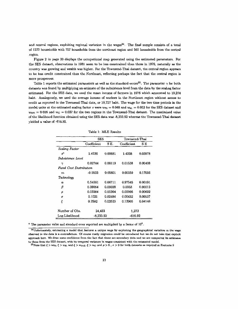
more prosperous.Table 1 reports the estimated parameters as well as the standard errors25. The parameter y for both

datasets was found by multiplying an estimate of the subsistence level from the data by the scaling factor

estimated. For the SES data, we used the mean income of farmers in 1976 which amounted to 19,274

baht. Analogously, we used the average income of workers in the Northeast region without access to

credit as reported in the Townsend-Thai data, or 10,727 baht. The wage for the two time periods in the

model units at the estimated scaling factor s were W7 6 = 0.048 and w8l = 0.053 for the SES dataset and

WNE = 0 016 and wc = 0.037 for the two regions in the Townsend-Thai dataset. The maximized value

of the likelihood function obtained using the SES data was -8,233.92 whereas the Townsend-Thai dataset

yielded a value of -616.92.

Table 1: MLE Results

SES Townsend-Thai

Coefficient S E. Coefficient S E

Scalmng Factorsa 1.4236 0.00881 1.4338 0.03978

Subsistence Level

-y 0.02744 0.00119 0.01538 0.00408

F7:red Cost Dtstributon

m -0 5933 0 05801 0.00559 0.17056

Technologyca 0.54561 0.06711 0.97545 0.00191

1B 0.39064 0.09028 0.0033 0.00013

p 0.03384 0.00364 0.00966 0.00692

or 0.1021 0.02484 0.00432 0.00157

0.2582 0.03523 0.12905 0.04146

Number of Obs. 24,433 1,272

Log-Likelihood -8,233.92 -616.92

The parameter value and standard error reported are multiplied by a factor of 106.

24Unfortunately, estimating a model that, features a unique wage by exploiting the geographical variation m the wage

observed in the data is a contradiction. Of course costly migration could be introduced but we do not take that explicit

approach here. We draw some confidence from the fact that these are secondary data and we are comparing its estimates

to those from the SES dataset, with its temporal variation in wages consistent with the estimated model.2 5Note that e > "u76, C > W8i and ( > wNE, C > wC and p >0 , a > 0 for both datasets as required in Footnote 9

13

From the standard errors one can construct confidence intervals. Indeed, they reflect the curvature

of the likelihood function at the point estimates and hence they also reveal the potential for errors in

the convergence to a global maximum. The magnitude of the standard errors, however, tell us little

about how sensitive the dynamics of the model are to the parameters. In Section 8 below we address

this issue by performing a sensitivity analysis. It is also interesting that both estimates of m fall withinthe permitted boundaries. Related, the SES data estimate of the parameter m implies a distribution of

talent more skewed towards low cost agents.

6 (Calibration

We still need to pin down the cost of living v and the "dynamic" parameters, namely, the savings rate w

and the subsistence income growth rate Ygr. One way to determine these parameters is calibration: look

for the best v, w and 'yr combination according to some metric relating the dynamic data to be matched

with the simulated data.In this section we first discuss the Thai macro dynamic data that will be used to calibrate the model

and then discuss some issues concerning the calibration itself.

6.1 Data

The Thai economy from 1976-1996 displayed nontrivial growth with increasing (and then decreasing)

inequality. LEB and related models are put forward in the literature as candidate qualitative explanations

for this growth experience. Here we naturally go one step further and ask whether the LEB model at

some parameter values can match quantitatively the actual Thai economy, focusing in particular on the

time series of growth, labor shares, savings rates, fraction of entrepreneurs, and the Gini measure of

income inequality. The actual Thai data are summarized in Table 2 in the Appendix.

The data show an initially high net growth rate of roughly 8 percent in the first three years. This then

fell to a more modest 4 percent up through 1986. The period 1986-1994 displayed a relatively high and

sustained average growth of 8.43 percent, and within that, from 1987-1989 the net growth rate was 8.83

percent. During this same period, the Thai economy GDP growth rate was the highest in the world at

10.3 percent. These high growth periods have attracted much attention. Labor share is relatively stable

at 0.40 and rising after 1990, to 0.45 by 1995. A trend from the 1990-1995 data was used to extrapolate

labor share for 1996. Savings as a percent of national income were roughly 22 percent from the initial

period to 1985. Savings then increased after 1986 to 33 percent, in the higher growth period. These

numbers, though typical of Asia, are relatively high. The fraction of entrepreneurs is remarkably steady,

though slightly increasing, from 14 percent to 18 percent. The Gini coefficient stood at 0.42 in the 1976

SES survey and increased more or less steadily to 0.53 in 1992. Inequality decreased slightly in both the1994 and 1996 rounds, to 0.50. This downward trend mirrors the rise in the labor share during the sameperiod, and both may be explained by the increase in the wage rate. This level of inequality is relatively

high, especially for Asia, and rivals many countries in Latin America (though dominated as usual byBrazil). Other measures of inequality, e.g., Lorenz, display similar orders of magnitude within Thailand

over time and relative to other countries26.26

The mterested reader will find a more detailed explanation in Jeong (1999).

14

The fraction of population with access to credit in 1976 was estimated at 6 percent and increased by

1996 to 26 percent. The data also reveal that as measure of financial deepening, it grew slowly in the

beginning and from 1986 grew more sharply. We recognize that at best this measure of intermediation is

a limited measure of what we would like to have ideally, and it seems likely we are off in levels.

6.2 Issues in the calibration method

6.2.1 Financial Liberalization

We begin with the standard, benchmark LEB model, shutting down credit altogether. We then consider

an alternative intermediated economy, with two sectors, one open to credit and saving. Only labor is

mobile, hence a unique wage rate, whereas capital cannot move to the other sector. In other words, a

worker residing in the non intermediated sector may find a job in the credit sector, even though she will

not be able to deposit her wealth in the financial intermediary. The relative size27 of each sector is taken

to be exogenous and changing over time given by the fraction of people with access to credit reported in

Table 2 in the Appendix. As mentioned, this is our key measure of liberalization.

6.2.2 Initial wealth distribution

Relevant for dynamic simulations is the initial 1976 economy-wide distribution of wealth28. As mentioned

before, Jeong (1999) constructs a measure of wealth from the SES data using observations on household

assets and the value of owner occupied housing units.

6.2.3 The metric

Any calibration exercise requires a metric to assess how well the model matches the data. As an example,

the business cycles literature has focused on models that are able to generate plausible co-movements

of certain aggregate variables with output. Almost by definition, the metric requires that the economy

displayed by these models be in a steady state. Even though the economy we consider here eventually

reaches a steady state, we are interested in the (deterministic) transition to it, thus the metric put forth

as our objective function suffers from being somewhat ad hoc. In particular, we consider the normalized

sum of the period by period squared deviations of the predictions of the model from the actual Thai data

for the five time series29 displayed in Table 2 in the Appendix. We normalize the deviations in the five

variables by dividing them by their corresponding means from the Thai data. More formally,

5 1996 Z:F - e 2

C=E E W at t (25)s=l t=1976 2z.

27We assume that the intermediated sector, with its distribution of wealth, is scaled up period by period according to

the exogenous credit expansion. Alternatively, we could have sampled from the no-credit sector distribution of wealth and

selected the correspondung fraction to the exogenous expansion, but the increase is small and his would have made little

difference in the numerical computations.r8Smce this estimated measure of wealth is likely to differ in scale and units to the wealth reported in the Townsend-Thai

data, we allow for a different scaling factor to convert SES wealth into the model units. In other words, we use two scaling

factors when we calibrate the model using the parameters estimated with the Townsend-Thai data. One is estimated with

ML techniques and converts wealth and incomes reported in the data, whereas the other is calibrated and converts the SES

wealth measure used to generate the economy-wide initial distribution.2 9

Note that in computing the growth rate we lose one observation, so the time index in the formula given in (25) runs

from 1977 to 1996 for the growth rate statistic.

15

where zJ denotes the variable s, t denotes time, and w,t is the weight given to the variable s in year t.In order to focus on a particular period, more weight may be given to those years. Analogously, all the

weight may be set to one variable to assess how well the model is able to replicate it alone. All weightsare re-normalized so that they add up to unity. Finally, sim and ec denote respectively "simulated" and"Thai economy", and M., denotes the variable zJm ean from the Thai data.

We search over the cost of living v, subsistence level growth rate -g, and the bequest motive parameterw using a grid of 203 points or combinations of parameters 3 0.

All the statistics but the savings rate have natural counterparts in the model. We consider "savings"

the fraction of end-of-period wealth bequested to the next generation. The savings rate then is computed

by dividing this measure of savings by net income3l.

7 Resullts

In this section we present the simulation results using the calibrated and estimated parameters from bothdata sets.

7.1 Simulations using SES Data Parameters

We begin with the original LEB model without liberalization. If all periods and all variables are weighted

equally, the parameters which minimize the squared error metric are v = 0.079, w = 0.479 and 7g. = 0.042.Figure 3 in page 40 displays the model simulations against the actual Thai data displayed earlier.

The figures show how the model fails to explain the levels and changes in roughly all variables. Inthe simulation, the growth rate of income is flat at roughly 2 percent. Growth is driven mainly by theexogenous growth of the subsistence level which is set at 4.2 percent per year. Overall, the economy

shrinks in the early periods, and then by 1983 it grows at the wage level32. The simulated labor share isable to roughly match the trend displayed in the data, although it is always higher in levels. The simulatedsavings rate is decreasing at first and then slightly increasing, always at a higher level than the actual

data. Entrepreneurship in the model is somewhat low. The Gini coefficient is always decreasing and

terribly low, in contrast to the first increasing and then decreasing pattern that the Thai data exhibits.If we had tried to match the growth rate alone, we do somewhat better on that dimension. In fact, we

are able to replicate the low growth - high growth phases seen in the data. Figure 4 in page 41 displaysthe model simulations when we restrict attention to the growth rate. The calibrated parameters here arev = 0.074, w = 0.7 and -g, = .1. The improvement in the growth rate comes at the expense of increasingthe model's savings rate above one from 1985 onwards, far above the actual one. Labor share increases

sharply in the model, but not in the data. The income Gini coefficient and the fraction of entrepreneursare very poorly matched as both drop to zero. The reason for such drastic macroeconomic aggregates is

3 0As mention earlier, when we use the Townsend-Thai data, we also search over a grid of 20 scaling factors for the mitial

distribution of wealth.31More formally we can express the savings rate (in an economy without credit) as

Savings Rate = fB f'l W(b, x, w)dH(x, m)dG(b) (26)f5l f0 Y (b, x, w)dH(x, m)dG(b)

where income Y(b, x, w) is given by W(b, x, W) = Y(b, x, w) +b as expressed in equation (4). Note that for some parameters,

the savings rate may be larger than one.32

Smce the cost of living v is roughly 3 times the subsistence income -y, wage growth rate wvll always be lower than 7yrg

16

the choice of model parameters which try to match the growth rate of income. The subsistence sector

is so profitable relative to setting up a business that by 1988 all entrepreneurial activity disappears and

everyone in the subsistence sector earns the same amount. It is clear that focusing on the growth rate

alone has perverse effects on the rest of statistics

We now modify the benchmark model to mimic part of the Thai reality, allowing an exogenous increase

in the intermediated sector from 6 percent to 26 percent from 1976-1996 as described in Table 2 in the

Appendix. We weight each year and all the variables equally and search again for the parameters v, w

and 7gr, allowing the best fit of the five variables. The parameters are M = 0.026, w = 0.321 and ygr = 0.The corresponding graphs are presented in Figure 5, page 42.

The modified intermediated model's explanation of events differs sharply from that of the benchmark

without an intermediated sector. Now the model is able to generate simulated time series which track

the Thai economy more accurately. In the model, the growth rate of income is again lower than that of

the Thai economy. The model still starts with negative growth until 1984. The initial phase of negative

growth comes from an initial overly high aggregate wealth in the economy. But growth jumps to 5.4

percent by 1987. This high growth phase comes from the rapid expansion of credit during those years.Finally, the growth rate declines after 1987 monotonically, driven by the imposed diminishing returns

in the production function. The model matches remarkably well the labor share levels and changes,

especially after 1990 where they both show a steady rise. The savings rate is only closely matched for

the period 1987-1996. The model also predicts a slightly decreasing fraction of entrepreneurs until 1985

and then a steady increase from 8.7 percent in 1985 to 16 1 percent in 1995, resembling more the actual

levels. Finally, the Gini coefficient folows a slightly decreasing, then slightly increasing, and finally

sharply decreasing trend, starting at .481 in 1976, then .377 by 1985, increasing to .451 by 1991 and

declining again to .284 by 1996. Beneath these macro aggregates lie the model's underpinnings. Growth

after 1985 is driven by a steady decline out of the subsistence sector, with income from earned wages and

from profits steadily increasing to 1990. Profits per entrepreneur are particularly high. Then, with the

subsistence sector depleted entirely, the wage increases faster, and profits begin to decrease. Thus labor

share picks up and inequality falls.To isolate the role of credit, we can consider the same economy, at the same parameter values, but

without the intermediated sector. In such a no-credit benchmark economy, roughly 80 percent of the

labor force are still subsisters by 1996. In fact, this benchmark model is only capable of replicating the

savings rate. It under-predicts labor share, the Gini coefficient, and the fraction of entrepreneurs. Labor

share starts (low) at 7.7 percent and rises to 29.8 percent by 1988. The Gini coefficient declines from .462

in 1976 to .238 by 1988. From then onwards, both simulated series remain constant until 1996. Income

growth is very badly matched, starting low initially and converging from negative to zero growth rate

by 1996. The negative growth comes from a relative abundance of wealth in the economy: households

eat and save that wealth as they move toward the subsistence growth rate of zero. We conclude then

that the credit liberalization is solely responsible for the growth experience that the intermediated model

displays.

7.2 Simulations with Parameters from the Townsend-Thai Data

The simulation generated from the economy with no access to intermediation at the Townsend-Thai

parameters, displays similar characteristics to the one using the SES data parameters and hence is not

reported.

17

We now turn attention to the intermediated economy at these parameter values. If we weight each

year and all the variables equally, the calibrated parameters are v = 0.004, w = 0.267 and -ygr = .006.

The scaling factor chosen for the initial distribution is 15 percent of the one used to convert wealth using

in the ML estimation. The corresponding graphs are presented in Figure 6, page 43.

The model here also does well at explaining the levels and changes in all variables, even better than

above with the SES data. Striking in particular is the growth rate of income, which although somewhat

low in levels, tracks the Thai growth experience well. The model also does remarkably wel in matching

labor share and the Gini measure of inequality. It under-predicts, however, the fraction of entrepreneurs,

although it is able to replicate a positive trend. As usual, the model features a flatter savings rate

although it matches well the last subperiod, 1988-1996. Economy wide growth is driven primarily by

growth in the intermediated sector. That is where the bulk of the economy's entrepreneurs lie and a

relatively high number of workers, from both the intermediated and non-intermediated sector.

8 Sensitivity Analysis of MILE parameters

We address the robustness of the model in two ways. First, we change one parameter at a time and check

whether the new simulation differs significantly from the benchmark one. Alternatively, we could see how

sensitive the model is to changes in all the estimated parameters at the same time. We now explain each

approach in detail.From the estimated parameters and their standard errors, confidence intervals can be constructed3 3.

One can then set one parameter at a time to its confidence interval lower or upper bound while fixing the

rest of the parameters at their original values. Keeping the calibrated parameters also fixed, one can then

simulate the economy. When we do this, it becomes clear that the simulations are more sensitive to some

parameters than others. The reason is that some parameters are close to the value that would make the

constraints described in Footnote 9 bind. When we perturb these parameters by changing them to their

confidence interval bounds, we approach the constraints, so the model delivers very different dynamics.

This is especially true for the parameters p and (. In fact, the lower bound of the confidence interval for

p obtained from the Townsend-Thai dataset violates some of the restrictions that the model must satisfy

to be well-behaved. Indeed, the unconstrained labor demand is zero, in which case no agent wiUl ever

want to become an entrepreneur regardless of his setup cost x.

When we change the setup distribution parameter m beyond its confidence interval to its extreme

values of [-1, 1], and still fix the rest of the parameters, we obtain somewhat more distorted pictures

than if m were contained in the confidence interval. However, we do not obtain the cycles discussed by

Lloyd-EUis and Bernhardt.

From the confidence intervals of the estimated parameters, we draw at random 5,000 different sets of

parameter values. It turns out, by chance, that none violated the conditions in Footnote 9. Notice that

since we also vary the scale parameter s, we are examining sensitivity to the initial wealth distribution

when we use the SES dataset. Fixing the calibrated parameters at their original level, we run 5,000

simulations for each the SES and the Townsend-Thai dataset. We then compute the mean and standard

deviation at each date over these 5,000 simulations of each of the five variables. Figures 5 and 6 also

display (in dots) the 95 percent confidence intervals around the mean.

Figure 5 shows that income growth, the savings rate and the fraction of entrepreneurs are quite

33We construct standard asymptotic 95% confidence intervals using the norrnal distribution.

18

insensitive to changes in the parameters within the 95 percent confidence intervals. Labor share and the

Gini coefficient can potentially display different dynamics judging by the wider bands, especially after

1989 at the peak of the credit expansion. The reason for this diversity of paths depends on whether

or not the subsistence sector was completely depleted by 1996. If such was the case, then demand for

workers would drive up wages, increasing the labor share and reducing inequality. If, on the contrary,

such depletion did not occur, labor share would remain fairly stable and inequality could increase34 .

Similar to the SES data results, the confidence intervals in Figure 6 show that the savings rate and the

fraction of entrepreneurs are robust to changes in the parameters. Income growth is more sensitive than

its SES analogue, especially in the earlier years, 1976-1980 and after 1990. However, the bands shrink

during the period of high growth. This indicates that all parameter combinations delivered this high

growth phase. Finally labor share and the Gini coefficient were very simular to their SES counterparts.

We thus conclude that with the exceptions enumerated above, the model is robust to changes in the

estimated parameters within their confidence intervals. We are yet more confident that the upturn of the

Thai economy in the late 1980's could be attributed to the expansion of the financial sector.

9 Welfare Comparisons

We seek a measure of the welfare impact of the observed financial sector liberalization. As there can be

general equilibrium effects in the model from this liberalization, we need to be clear about the appropriate

welfare comparison. We shall compare the economy with the exogenously expanding intermediated sector

to the corresponding economy without an intermediated sector at the same parameter values. The

criterion will be end-of-period wealth - that is what households in the model seek to maximize. For

a given period, then, we shall characterize a household by its wealth b and beginning-of-period cost

* and ask how much end-of-period wealth would increase (or decrease) if that household were in the

intermediated sector in the liberalized economy, as compared3 5 with the same household in the economy

without intermediation, a restricted economy.

If in fact the wage is the same in the liberalized and restricted economies, then this is also the obvious,

traditional partial equilibrium experiment - a simple comparison of matched pairs, each person with the

same (b, x) combination but residing in two different sectors of a given economy, one receiving treatment

in the intermediated sector and one without it. The wage is the same with and without intermediation

in both SES and Townsend-Thai simulations before 1990, when the subsistence sector is not depleted.

If the wage is different across the two economies, this latter comparison does not measure the net

welfare impact of the liberalization. Rather it measures end-of-period welfare differences across sectors of

a given economy that has experienced price changes. To be more specific, those in the non-intermediated

sector of the liberalized economy will experience the impact of the liberalization through wage changes

- workers in the non-intermediated sector may benefit from wage increases while entrepreneurs in the

non-intermediated sector suffer losses, since they face a higher wage. And of course there is a similar

price impact for those in the intermediated sector, but there is a credit effect there as well. There are

such wage effects using the parameters estimated from both datasets after 1990.

'This dichotomous feature of the model could be improved by imposing diminishing returns in the subsistence sector.35We could compare the end-of-period wealth of a given household with (b, x) in the non-intermediated sector of the

intermediated economy with the same (b,x) household in the non-intermediated economy This would decompose the

welfare gains (and losses).

19

Implicit in this discussion is another problem which has no obvious remedy here, given the model.

Although households in the model maximize end-of-period wealth, they pass on a fraction of that wealth

to their heirs. Thus the end-of-period wealth effects of the liberalization are passed onto subsequent

generations. The problem is that there is no obvious summary device - households do not maximize

discounted expected utility, as in Greenwood and Jovanovic (1990) and the analysis of Townsend and

Ueda (2001), for example. Here then we do not attempt to circumvent the problem but rather present

the more static welfare analysis for various separate periods. A related issue is the difficulty of weighting

welfare changes by the endogenous and evolving distributions of wealth in the two economies -see below

for more specifics on that.

We take a look first at the liberalized economy in 1979, three years after the 1976 initial start up,

using the overall best fit Townsend-Thai data economy with liberalization. As noted earlier, the wage

has not yet increased as a result of the liberalization. Its value is .0198 in the liberalized and restricted

benchmark economies. The interest rate in the intermediated sector of the liberalized economy is very

high, at 93 percent. This reflects the high marginal product of capital in an economy with a relatively

low distribution of wealth.

Figure 7b in page 44 displays the corresponding occupation partition, but now denoting for given

beginning-of-period (b, x) combinations the corresponding occupation of a household in the no-credit

economy and in the credit sector of the intermediated economy. The darker shades of Figure 7b denote

households with (b, x) combinations who do not change their occupation as a result of the liberalization,

that is, they are entrepreneurs (E) in the no-credit (NC) economy and in the intermediated sector of

the liberalized (C) economy, or workers (W) in both instances. The light shades denote households who

switch: low wealth but low cost agents who were workers become entrepreneurs, and high wealth, high

cost agents who were entrepreneurs become workers. The picture is the overlap of the occupational maps

in both sectors. For the credit sector, the key parameter is z, whereas for the no-credit sector, it is the

curve xe(b, wo).

Figure 7a in page 44 displays the corresponding end-of-period wealth percentage changes in the same

(b, x) space. Since the wage is the same in both sectors, agents will only benefit from being in the

credit sector, not only because they can freely borrow at the prevailing rate if they decide to become

entrepreneurs, but because they can deposit their wealth and earn interest on it. The wealth gain due to

interest rate earnings can be best seen by fixing x and moving along the b axis, noting the rise.

If on the other hand we look at the highest wealth, b = 0.5 edge, we can track the wealth changes that

correspond to changing set up costs x. Going from the rear of the diagram, at high z, we see that the

wealth increment is constant, but these households were workers in both economies, so set up costs x are

never incurred. Then the wealth increment drops -these households were entrepreneurs in the no-credit

economy and were investing some of their wealth in the set up costs x- those with high x gain the most,

quitting that investment and becoming workers in the intermediated sector. Thus the percentage wealth

increment drops as x decreases. One reaches a trough, however, when the household decides to remain

an entrepreneur. Yet lower set up costs benefit entrepreneurs in the intermediated sector more than in

the corresponding no-credit economy, because the residual funds can be invested at interest. Hence, the

back edge rises up as x decreases further.

The most dramatic welfare gains, however, are experienced by those agents who are compelled to

be workers in the no-credit economy but become entrepreneurs in the intermediated sector. Although

their setup cost was relatively low, their wealth was not enough to finance it. They were constrained on

20

the extensive margin. When credit barriers are removed, they benefit the most. The sharp vertical rise

corresponds to those on the margin of becoming a entrepreneur in the no-credit economy. Intuitively,

this is because with their low x, they would have earned the highest profits if they could have been

entrepreneurs. Credit in the intermediated sector allows that.

A problem with this analysis, however, is that we may be computing welfare gains for household with

(b, x) combinations that do not actually exist in either the liberalized economy or the no-credit economy,

that is, have zero probability under the endogenous distribution of wealth. To remedy this, Figures 7c

and 7d also in page 44 display the wealth distributions of the no-credit economy and credit economy

(over both sectors) in 1979.

Figures 7f and 7h present a similar version, plotting the joint density level curves of the end-of-period

wealth levels in the no credit and liberalized sector36 . Those on the 45 degree line correspond to those

with no change in wealth. We use the endogenous end-of-period wealth distribution in both the credit

and no-credit sector and the distribution of x at the estimated tilt parameter m to weight each (b, x)

pair.We report last the density of percentage changes in wealth in Figures 7e and 7g also in page 44 by

integrating the 3D graph in Figure 7a over the estimated range of x and weighting each b point using both

the credit and no-credit wealth distribution3 7 . We recognize that the distribution of wealth is endogenous,

so taking any weighting is somewhat arbitrary. Still, when compared, they display a somewhat different

pattern. We can convert this relative wealth gain into 1997 baht for both weighting distributions. The

mean gain amounts to 61,582 baht using the no-credit distribution or 82,376 baht using the credit one.

These numbers correspond to roughly 1.5 times and twice the average household yearly 1979 income38

(measured in 1997 baht) respectively. The modal gains are significantly lower, 6,961 baht or 7,779 baht

if we use the no-credit or credit distribution, respectively, which amount to roughly 17 percent or 19

percent of the 1979 average household yearly income. In dollars, these gains become $278 or $311 using

the no-credit or credit distribution at the 1997 exchange rates.

By 1996, the wage has risen to 0.022 in the non-intermediated economy and to 0.029 in the inter-

mediated one. The interest rate in the intermediated sector has fallen to 57 percent. The occupation

partition diagram has no agents who were entrepreneurs becoming workers (though that number was

never large). In contrast, the relative number of those who were workers and become entrepreneurs is

higher. The three dimensional diagramn in Figure 8a in page 45 of wealth changes is still tilted upward

towards high wealth, due to the interest rate effect. On the back edge, at the highest wealth shown,

wealth increments are positive and constant for those who stay as workers, both due to higher wages and

interest rate earnings, but those who were workers and become entrepreneurs have high wealth gains,

which increases as x falls, since net profits of entrepreneurs increases as setup costs falls and funds can

be put into the money market. However, one reaches a point where they would have been entrepreneurs

in both economies, incurring x in both economies, and then the wealth gains though increasing as x

decreases are relatively small or negative. Note that on the one hand, entrepreneurs in the intermediated

sector face higher wages, obtaining lower profits. On the other, they are able to collect interest on their

38The joint density is approximated using kernel density estimation, from a generated sample of 10,000 points The kerrnelused is Epanechnikov. See Silverman (1986) for details. Some level curves fall below the 45°li ne, but this is an artifactof the kernel density estimation which tends to oversmooth. Figure 7a assures us that the liberalization only improves thewelfare. Each contour level represents an increased density of 0.01, starting at 0.0025

37The density is approximated by the techniques explained in Footnote 363The 1979 average household yearly income is estimated from the SES data. Since we do not have actual SES data m

1979, we interpolate it using the average annual growth rate between 1976 and 1981

21

wealth. These opposing wealth effects will translate into net gains or losses depending on their relative

magnitude. More salient, the former tent-shaped region has pervaded this graph - the biggest gainers

throughout the entire distribution of wealth are those on the margin of indifference between staying as a

worker or becoming an entrepreneur in the non-intermediated economy.

The distributions of wealth of the no-credit and intermediated sector are also plotted in Figures 8c

and 8d in page 45. Note that the scale has changed. Evidently both are more compressed from what

they had been in 1979. Applying those distributions as weights to the diagrams with level wealth changes

around the 45 degree line, one sees that again those at the low end of wealth would be measured as

having extraordinary gains, from zero to ten-fold or more, and again in the credit economy a richer

class gains somewhat from the yet high interest rates. The mean welfare gains of those who benefit

from the liberalization amount to 52,573 baht or 65,789 1997 baht if we use the No-Credit or Credit

distribution, respectively. The modal gains are lower at 6,863 baht or 15,905 baht using the No-Credit

and Credit distribution. They correspond to roughly 9 percent and 21 percent, respectively, of the 1996

yearly household income as reported in the SES data. If we translate these modal gains into dollars, we

obtain $275 or $636 per year. However, there is also a nontrivial fraction of entrepreneurs who end uplosing due to higher wages. The mean losses for this subset of the population amount to 9,509 baht using

the No-Credit distribution or 34,816 baht using the Credit distribution. They correspond to roughly 9

percent and 32 percent of the 1996 average household yearly income for the sample of entrepreneurs. In

dollars, these losses become $380 and $1,393 using the No Credit and Credit distribution, respectively.

We now turn to the welfare comparison from the simulation using the best fit estimated MLE param-

eters using the SES data. The first thing to notice is that reported welfare gains are much lower. Two

years after the outset of the liberalization, 1978, both economies have the same wage, and therefore the

credit liberalization only improves the welfare of those who can take advantage of it. The 3D Figure 9a in

page 46 resembles somewhat that of 1979 using the parameters estimated from the Townsend-Thai data.

It is titled upward as we move along the b axis due to interest earning gains and again, the big winners

are those who could not afford the set up cost (even though it was low) and had to take a job as a worker.

If credit were available to them, they would become entrepreneurs, realizing huge profits, amounting to

an increase in their wealth by a factor of up to nine-fold. The kernel density estimates in Figure 9e and

9g in page 46, however, show that the average wealth increase is somewhat lower, around 100 percent.

These correspond to a mean wealth gain of 102,586 baht or 90,785 baht if we use the no-credit or credit

distribution, respectively. The modal gains are again much lower, 5,560 baht for the no-credit or 17,000

baht for the credit distribution. These correspond to $222 or $680 at the 1997 exchange rate or, roughly

14 percent or 41 percent of the average household yearly income in 1978.

In 1996, the 3D Figure lOa in page 47 shows that welfare gains are somewhat smaller. Those agents

that remain workers in the credit sector are better off because they earn a higher wage, and those that

become entrepreneurs in both sectors end up losing because they face higher labor costs. As in the

Townsend-Thai dataset, if we look at the distribution of welfare gains in Figures 10e and 10e, page 47,

there is a significant fraction of agents who end up losing about half of their annual wealth. The average

wealth gain is still positive at around 100 percent if we use the no-credit wealth distribution and around

80 percent if we use the credit one. But both distributions have negative support, a result of the fact that

agents benefit in diverse ways from the credit liberalization. The mean welfare gains for those who benefit

from the liberalization are 83,444 1997 baht or 76,840 1997 baht for the no-credit and credit distribution,

respectively, and correspond to 1.09 times or one time the 1996 average household yearly income. The

22

modal welfare gains of those who gain are roughly 18,591 baht or 25,655 under the no-credit and credit

distributions which correspond to roughly 24 percent and 34 percent of 1996 average household yearly

income, equivalent to $1,030 at the 1997 exchange rate. The mean losses, for those worse off are 115,861

baht or 117,051 using the no-credit and credit distributions respectively, which amounts to 1.06 times or

1.08 times the average household yearly income for the sample of entrepreneurs, or roughly $4,650 using

again the 1997 exchange rate.

10 Extensions: International Capital Inflows and Alternative

Credit Regimes

In this section, we explore two important extensions to the model. These may be viewed as robustness

checks to the results presented in the previous sections. The first concerns the liberalization of the capital

account that Thailand experienced, especially after 1988. The second relaxes the assumption of restricted

credit to allow for some external financing. We now take each one in turn.

Figure 11 in page 48 displays the capital inflows as a fraction of GDP. The data come from the Bank

of Thailand as reported in Alba, Hernandez and Klingbiel (1999). From 1976 to 1986, private capital

inflows to Thailand remained relatively low at an average of 1.05% of GDP. From 1986 to 1988, however,

they increased rapidly to 10% of GDP, remaining at that average level until 1996.

This enhanced capital availability was funnelled through the financial sector and thus it is modelled

here as additional capital for those households that have access to the financial market (i.e. residing in

the credit sector). We run this extended (open) version of the model at the estimated and calibrated

parameters and compare it to the previous closed credit economy model at the same estimated and

calibrated parameter values from the two datasets39 . Although not shown, capital inflows contribute to

a larger number of entrepreneurs, and larger firm size, in particular in the late 80's and early 90's. Since

the marginal product of labor increases with capital utilization, more labor is demanded and thus the

fraction of subsisters is depleted earlier. Thus labor share rises and inequality decreases, both relative to

the actual path and relative to the earlier simulation. The interest rate tends to be lower with capital

inflows. Nevertheless, the welfare changes are small, indeed, almost negligible.

Because the surge in capital inflows coincides with the phase of high growth of per capita GDP, it has

often been portrayed as an important factor contributing to that high growth. In order to disentangle

the extent to which the phase of high growth was due to increased participation in the credit market

versus additional capital availability due to capital account liberalization, we simulate the economy at the

estimated and calibrated parameter values allowing for international capital inflows but using a linearized

credit participation from 6% to 26%, that is, a one percent increase per year for each of the 20 years. As

displayed in Figure 12, page 48, this version of the model fails to match the upturn in GDP growth as

compared to the benchmark credit economy. Thus, it seems from the model that capital inflows per se

were not the cause of the high growth that Thailand experienced in the late 80's.

The assumption of restricted credit may artificially deliver quantitatively large welfare gains from

liberalization if those assumed to have no access were in fact able to receive some credit, perhaps from

391n addition, we re-calibrated the cost of living v, subsistence level growth rate 7gr and the bequest motive parameterw for this open economy version and found even fewer differences compared to the closed economy model. In particular,the calibrated bequest motive parameter w is lower for both datasets in the open economy version, so that the depletion ofsubsisters happens at a slower rate.

23

informal sources. Indeed, in the model so far, we have not allowed any form of lending (formal or informal)

for those households residing in the no-credit sector. We now relax that assumption and explore whether

the welfare gains from liberalization would differ significantly from those reported in the previous section.

We follow Lloyd-Ellis and Bernhardt (2000) and introduce intermediation which is limited by a moral

hazard problem4 0. In particular, given an interest rate of r, possibly different from that in the formal

sector, entrepreneurs borrow L and put up their wealth b as collateral. After production they can abscond

losing rb but escaping the repayment obligation rL. Absconders are apprehended with probability p and

if so they can hide their income but receive a punishment corresponding to an additive disutility of d.

Borrowers will renege on the loan contract if rb + pd < rL, so lenders only make loans that satisfy

L < b + A, where A = pd/r. Thinking again about help from friends and relatives, we set r = 1 so

that the objective function for households that now can "borrow" from the informal sector is the same

as before. However, the constraint in (3) is now modified to

k+z <b+A.

In effect, parameter A is treated as a lump sum addition to wealth but only for those who borrow from

the informal sector and choose to start firms This would allow more talented households to alleviate

credit constraints 41.As shown in the Appendix, parameter A would be identified in cross sectional maximum likelihood

estimation. However, to give parameter A a greater opportunity to influence the dynamic paths relativeto the earlier simulation, we calibrate the parameter A against the dynamic aggregate data for each

dataset using the previously estimated and calibrated parameter values for the other parameters. The

calibrated values of parameter A are A = 0.0163 for the Townsend-Thai dataset and A = 0.0082 for the

SES dataset. These correspond to 1.1 times and 30% of the subsistence income in 1976 for each dataset

respectively.Similarly to the open economy version, the increased informal finance speeds up the creation of firms

resulting in an earlier depletion of the fraction of subsisters. Again, labor share begins to increase along

with a decline in the Gini coefficient, both at an earlier date.

Although the parameter A could in principle have a large welfare impact, at the calibrated parameterA that best fits the Thai economy, these welfare gains and losses remain much as before. In particular,

the counterparts of Figures 7a - lOa in pages 44-47 still feature the tent-shaped gains for relatively

talented but poor people. Recall that in the intermediated sector, only the most talented individuals will

start a firm, irrespective of their wealth. However, even when we relax the constraint in the no-credit

sector by alowing informal finance, wealth still matters in determining who becomes an entrepreneur,

and thus the tent-shaped welfare gains still appear. In addition, the increased wage in the latter periods

does benefit workers in the liberalized economy. In the no-credit economy which now has informal credit,

some households become richer but the additional capital from informal sources is insufficient to trigger

an increase in the equilibrium wage rate. Thus, in the welfare experiment comparing the intermediatedto the no-formal-credit economies, wage earners benefit more from the liberalization, but not much. In

contrast, firms lose from the relative increase in the wage, but not much.

40We also tried modifying the constraint in (3) to k E i4O, b - xz, where the parameter N. measures the severity of the

financing constraints. Thus, if some of the assets that make up wealth are illiquid, we would expect rN < 1. Unfortunately,

this specrfication is not useful because the parameter N cannot be identified.4t

We are implicitly assuming a partial equilibrium, unlimited supply of funds by setting r = 1. However, the magnitude

of the calibrated parameter A as reported below is comparable to the average amount of informal borrowing found in the

Townsend-Thai dataset by those households who borrow informally.

24

A prediction of the model that could seemingly be checked in the data concerns rates of return to

capital. One might suppose that with limited credit the rate of return to capital would be high. This is

true for some firms in the simulations. However, for other firms without access to intermediation, wealth

cannot be lent at interest and is thus invested internally at low rates of return. Thus the implication of

the model is unclear about the mean, average rate of return to capital and only asserts that the dispersion

of rates of return is higher for firms without access relative to those who can borrow and lend.

11 Conclusions

From the welfare numbers presented, there seems to be a lot at stake in credit liberalizations. Even by our

most conservative estimates there is a group of low wealth talented households who have much to gain,

period by period, in income and wealth. On the other hand, the estimates reveal a group of entrepreneurs

who have much to lose, period by period, in income and wealth, particularly if one takes into account

the growth in wages. We do not push here any particular any number as the most compelling, because

the numbers do vary and do depend on the dataset used. Indeed, the larger point is that welfare gains

and losses are sensitive to the presumed, estimated micro underpinnings of the economy. If there were

more substantial intermediation, then variations associated with further liberalization would matter less

Indeed, if there were more substantial intermediation, then the impact on dynamics of (endogenous)

changes in the wealth distribution would matter less, as in Krusell and Smith (1998). But the micro data

reject such presumed underpinnings, making welfare gains, potential losses, and the dynamic aspect of

liberalization more substantial.

Still, the surprisingly large order of magnitude of these gains and losses suggests the need for further

refinements along a number of dimensions, to see if the magnitude survives somewhat more realistic

specifications.One refinement has to do with labor and the labor market. The labor of the model here is uniform

with respect to productivity, that is, every laborer earns the same wage. This ffies in the face of much

empirical work mapping wage differentials to skills differentials and acquired human capital. More gen-

erally, earnings inequality contributes to overall inequality, and this might be salient, as in the work of

Ricardo Paes de Barros in Brazil, for example. Jeong and Townsend (2000) document the success and

failure of the LEB model in explaining inequality movements in Thailand, comparing it to an extended

version of Greenwood and Jovanovic (1990). Though the LEB model at the maximum likelihood parame-

ter estimates does surprisingly well, it is clear that wage differentiation is needed in models and in model

based empirical work. In the model of occupation choice of Evans and Jovanovic (1989), for example,

unobserved heterogeneous skills influence both wage earnings and the profits from entrepreneurship. This

might suggest that entrepreneurs worry less about increased wages as they potentially exit to become

part of a skilled work force.

Second, one could endogenize access to credit as in the Greenwood and Jovanovic (1990) model with

transactions costs. This would slow down the growth of financial infrastructure and would rationalize

some of the limited participation that we see but there would be no Pareto-improving policy intervention.

However, Townsend and Ueda (2001) in an extended version of the Greenwood and Jovanovic model draw

the conclusion that restrictive financial sector policies may have nevertheless slowed down entry into the

financial sector below the endogenous rate. Thus financial sector liberalization, allowing intermediation

at its otherwise endogenous value, is also associated with welfare gains, as in this paper Although

25

occupation choice models should allow more endogenous financial sector participation, they illustratewell as they stand the fact that there may be welfare losses for some sectors of the population, not justgains, to liberalization. This offers a political economy rational for the apparently restrictive policies thatwe observed in Thailand.

Third, the imagined industrial organization of the Thai economy is relatively simple. In the modelhere fixed setup costs are allowed to vary across potential entrepreneurs, as if drawn from a quadraticcumulative distribution, but the quadratic production function mapping labor and capital into output isuniform across potential entrepreneurs. This delivers the occupation partition diagram and variation overtime in the size distribution of firms, a function of the wage and the endogenous distribution of wealth.Indeed, an industrial organization literature starting with Lucas (1978) begins the same way, at leastin spirit. He postulates an underlying distribution of personal managerial talent and then studies thedivision of persons into managers and employees and the allocation of productive inputs across managers.This has implications for secular changes in average firm size. This point is revisited by Gollin (1999).

Here the distribution of size and profits among firms is driven by self-financing, an endogenous andevolving distribution of wealth, and differential access to credit. That is, high set up costs and limitedcredit can limit the use of real physical capital in the standard part of the production function or canimpede entry entirely. Likewise, some portion of end-of period profits is passed on to subsequent timeperiods if not subsequent generations. This could be an explanation for some of the serial correlation insize, profits, and employment that is seen in actual data, even when shocks in the form of set up costsare independent and identically distributed over time and households There would be implications forthe cross-sectional dispersion in growth rates. Indeed, it seems that in Thailand larger firms, and thosewith financial access, may have grown faster than smaller ones as the credit market expanded in thelate 1980's. Recent theoretical work is beginning to readdress earlier the supposed facts of firm growthand survival in the context of endogenous limited financial contracts. See Albuquerque and Hopenhayn(2001) and Cooley, Marimon and Quadrini (2000)

More generally both the industrial organization and credit market literature need to be broughttogether. Existing empirical work has documented relationships between investment and the balancesheet, for example, but much of this work is somewhat atheoretic, documenting that the world is notneoclassical but leaving us wondering what the impediments to trade really are. The general equilibriummodels of Banerjee and Newman (1993), Piketty (1997) and Aghion and Bolton (1997) take differentstands on those underpinnings but collectively make the point that growth and inequality can be relatedto imperfect credit markets. That of course was our starting point here.

Indeed, in related work Paulson and Townsend (2001) use the Townsend-Thai data to estimate viamaximum likelihood methods not only the LEB model featured here, but also collateral based lendingas in model of Evans and Jovanovic (1989) (EJ for short), for example, and also incentive-based lendingas in the mechanism design literature of Aghion and Bolton (1997) and Lehnert (1998) (ABL for short).Observed relationships of entrepreneurship, investment, and access to credit as functions of wealth andtalent suggest that the ABL model fits the micro Thai data best, but the EJ model fits well for thosewith relatively low levels of wealth and those in the Northeast, while LEB, the model here, is a closecontender. This suggests that a calculation of the welfare gains and losses to financial intermediationbased on these other models would be worthwhile, though the average and modal estimates here shouldnot be rejected out of hand. It does seem plausible, however, that the dramatic gains near the wealthequal set-up costs or 45° line would be vulnerable to alternative specifications.

26

The growth and inequality literature relying on each of these underpinnings presupposes, as in the

LEB model here, either an overlapping generations model with a bequest motive or a simplistic, myopic

solution to the household savings problem. More needs to be done to make the models dynamic. Coupling

households with firms and modelling the firms' inter-temporal decision problems will require more work,

but again, given the prelinminary results here, that work would appear to be warranted.

27

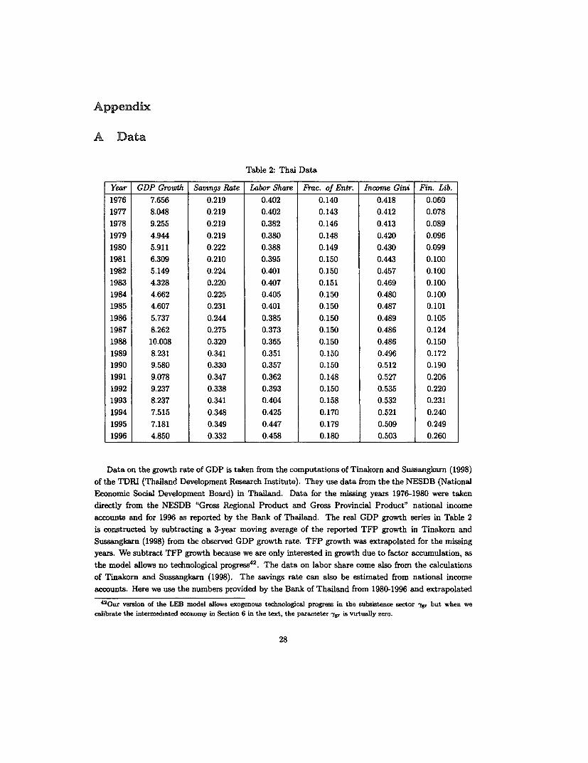
Appendix

A Data

Table 2: Thai Data

Year GDP Growth Savings Rate Labor Share Frac. of Entr. Income Gini Fin. Lib.1976 7.656 0.219 0.402 0.140 0.418 0.0601977 8.048 0.219 0.402 0.143 0.412 0.0781978 9.255 0.219 0.382 0.146 0.413 0.0891979 4.944 0.219 0.380 0.148 0.420 0.0961980 5.911 0.222 0.388 0.149 0.430 0.0991981 6.309 0.210 0.395 0.150 0.443 0.1001982 5.149 0.224 0.401 0.150 0.457 0.1001983 4.328 0.220 0.407 0.151 0.469 0.1001984 4.662 0.225 0.405 0.150 0.480 0.1001985 4.607 0.231 0.401 0.150 0.487 0.1011986 5.737 0.244 0.385 0.150 0.489 0.1051987 8.262 0.275 0.373 0.150 0.486 0.1241988 10.008 0.320 0.365 0.150 0.486 0.1501989 8.231 0.341 0.351 0.150 0.496 0.1721990 9.580 0.330 0.357 0.150 0.512 0.1901991 9.078 0.347 0.362 0.148 0.527 0.2061992 9.237 0.338 0.393 0.150 0.535 0.2201993 8.237 0.341 0.404 0.158 0.532 0.2311994 7.515 0.348 0.425 0.170 0.521 0.2401995 7.181 0.349 0.447 0.179 0.509 0.2491996 4.850 0.332 0.458 0.180 0.503 0.260

Data on the growth rate of GDP is taken from the computations of Tinakorn and Sussangkarn (1998)of the TDRI (Thailand Development Research Institute). They use data from the the NESDB (NationalEconomic Social Development Board) in Thailand. Data for the missing years 1976-1980 were takendirectly from the NESDB "Gross Regional Product and Gross Provincial Product" national incomeaccounts and for 1996 as reported by the Bank of Thailand. The real GDP growth series in Table 2is constructed by subtracting a 3-year moving average of the reported TFP growth in Tinakorn andSussangkarn (1998) from the observed GDP growth rate. TFP growth was extrapolated for the missingyears. We subtract TFP growth because we are only interested in growth due to factor accumulation, asthe model allows no technological progress42 . The data on labor share come also from the calculationsof Tinakorn and Sussangkarn (1998). The savings rate can also be estimated from national incomeaccounts. Here we use the numbers provided by the Bank of Thailand from 1980-1996 and extrapolated

420ur version of the LEB model allows exogenous technological progress in the subsistence sector yg, but when wecalibrate the intermediated economy in Section 6 in the text, the parameter -g, is virtually zero.

28

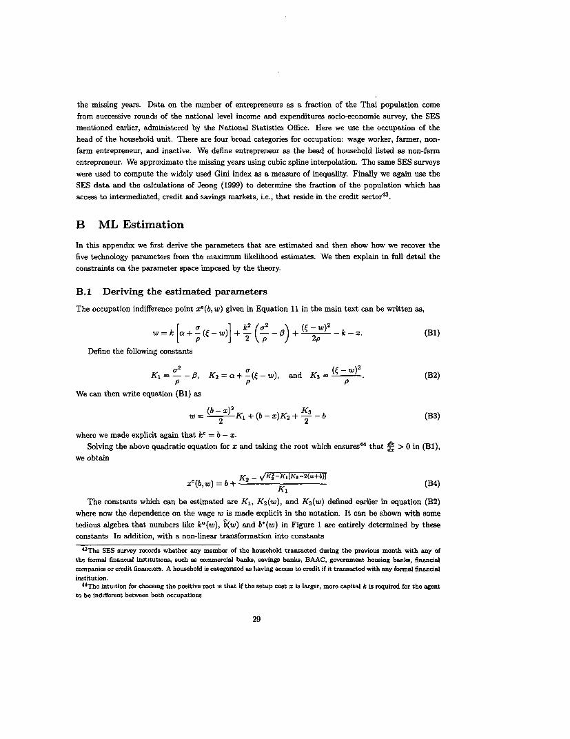
the missing years. Data on the number of entrepreneurs as a fraction of the Thai population come

from successive rounds of the national level income and expenditures socio-economic survey, the SES

mentioned earlier, administered by the National Statistics Office. Here we use the occupation of the

head of the household unit. There are four broad categories for occupation: wage worker, farmer, non-

farm entrepreneur, and inactive. We define entrepreneur as the head of household listed as non-farm

entrepreneur. We approximate the missing years using cubic spline interpolation. The same SES surveys

were used to compute the widely used Gini index as a measure of inequality. Finally we again use the

SES data and the calculations of Jeong (1999) to determine the fraction of the population which has

access to intermediated, credit and savings markets, i.e., that reside in the credit sector 43.

B ML Estimation

In this appendix we first derive the parameters that are estimated and then show how we recover the

five technology parameters from the maximum likelihood estimates. We then explain in full detail the

constraints on the parameter space imposed by the theory.

B.1 Deriving the estimated parameters

The occupation indifference point xe(b, w) given in Equation 11 in the main text can be written as,

F u 1 k CF2 _\3 ( -W)2

-k-x

w = k [a +- (-w)j + 2- (-- x) + 2 (B1)

Define the following constants

K, = ap -, K2 = +-a(C-w), and K3 = (1-w). (B2)p p p

We can then write equation (B1) as

w = (2)K + (b-z)K2 + K3-b (B3)

where we made explicit again that kc = b -.

Solving the above quadratic equation for x and taking the root which ensures44 that dk > 0 in (Bi),

we obtain

K( -+X =fK~-i Ks-2(v+b)l B4x'(b, w) = b + K2 - K --- -- 7 (B4)

The constants which can be estimated are K1 , K2 (w), and K3(w) defined earlier in equation (B2)

where now the dependence on the wage w is made explicit in the notation. It can be shown with some

tedious algebra that numbers like ku(w), b(w) and b'(w) in Figure 1 are entirely determined by these

constants In addition, with a non-linear transformation into constants

4 3 The SES survey records whether any member of the household transacted during the previous month with any of

the formal financial institutions, such as commnercial banks, savings banks, BAAC, government housing banks, financial

companies or credit financiers. A household is categorized as having access to credit if it transacted with any formal financial

institution."The intuition for choosing the positive root is that if the setup cost x is larger, more capital k is required for the agent

to be indifferent between both occupations

29

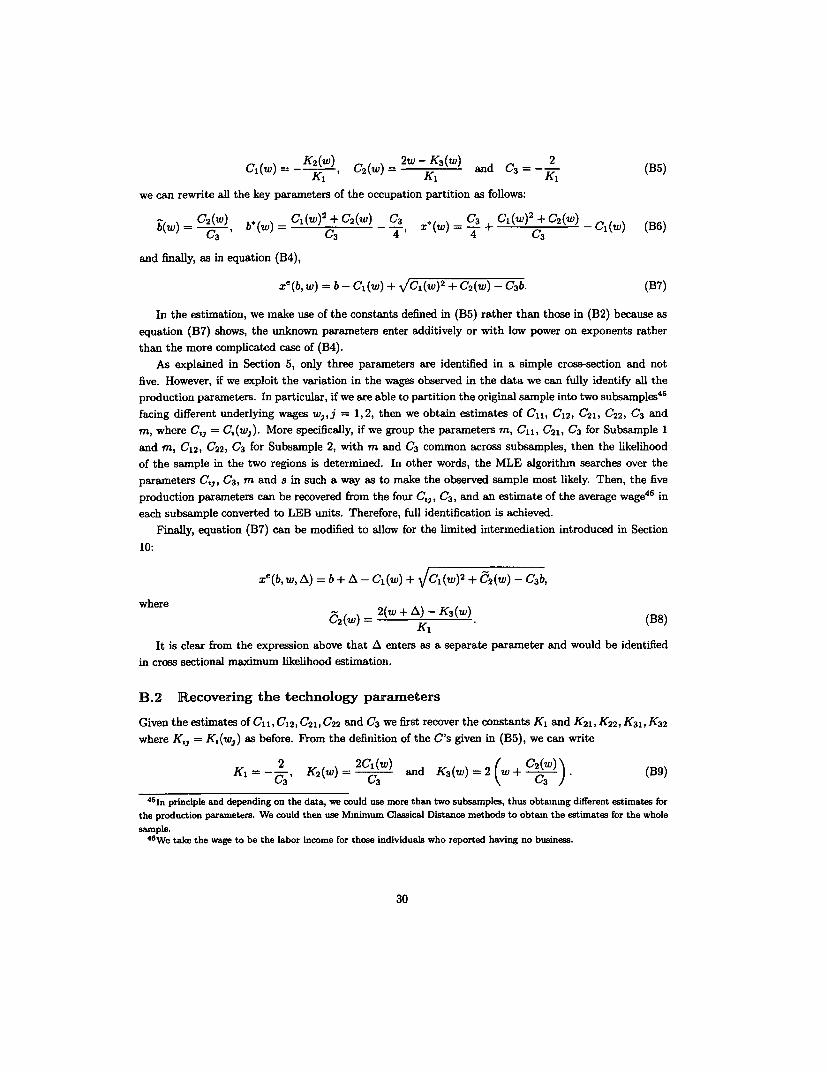
Cl( = K2 (w) = 2wK3() and C3 =-- (B5)K1 ~~~~~K1 K1

we can rewrite all the key parameters of the occupation partition as follows:

(w) = C2 (w), b (w) = C()+C 2 () _ C3 (W)=C 3 + C1 (W) 2 -+C2 (W)

and finally, as in equation (B4),

xe(b, w) = b - C(w) + VCi(w)2 + C2 (w) - C3b. (B7)

In the estimation, we make use of the constants defined in (B5) rather than those in (B2) because asequation (B7) shows, the unknown parameters enter additively or with low power on exponents ratherthan the more complicated case of (B4).

As explained in Section 5, only three parameters are identified in a simple cross-section and notfive. However, if we exploit the variation in the wages observed in the data we can fully identify all theproduction parameters. In particular, if we are able to partition the original sample into two subsamples45

facing different underlying wages w,,j = 1,2, then we obtain estimates of Cll, C1 2 , C2 1 , C2 2 , C3 andm, where C, = C,(w,). More specifically, if we group the parameters m, C1l, C21, C3 for Subsample 1and m, C12, C22, C3 for Subsample 2, with m and C3 common across subsamples, then the likelihoodof the sample in the two regions is determined. In other words, the MLE algorithm searches over theparameters C,,, C3, m and s in such a way as to make the observed sample most likely. Then, the fiveproduction parameters can be recovered from the four C,,, C3, and an estimate of the average wage4" ineach subsample converted to LEB units. Therefore, full identification is achieved.

Finally, equation (B7) can be modified to allow for the limited intermediation introduced in Section10:

xe(b, w, A) = b + A-C,(w) + VCI(w)2 + C 2(w)-C 3 b,

where 2w+A 3W

rC2(W) = 2(7+A)-Ks(w) (B8)

It is clear from the expression above that A enters as a separate parameter and would be identifiedin cross sectional maximum likelihood estimation.

B.2 Recovering the technology parameters

Given the estimates of Cll, C1 2, C21, C22 and C3 we first recover the constants K1 and K2 1, K22 , K31 , K32

where K,, = K,(w,) as before. From the definition of the C's given in (B5), we can write

K, = -C XK() = C( ) and K3(w) = 2 ( + C )). (B9)~~3 ~ C3 W C )

451n principle and depending on the data, we could use more than two subsamples, thus obtaining different estimates forthe production parameters. We could then use Mmimum Classical Distance methods to obtain the estimates for the wholesample.

46We take the wage to be the labor income for those individuals who reported having no business.

30

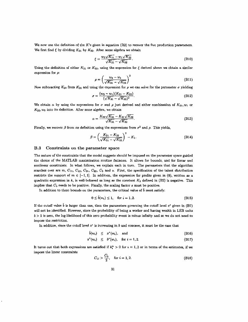
We now use the definition of the K's given in equation (B2) to recover the five production parameters.

We first find C by dividing K31 by K32. After some algebra we obtain

w2Y31- wv32

Using the definition of either K31 or K32, using the expression for C derived above we obtain a similar

expression for p:

P=( W2 - WI Bl'= ~~~~~~~~~~~~(Bil)

Now subtracting K22 from K21 and using the expression for p we can solve for the parameter e yielding

e (W2 - W)(K 21 - K2 2) (B12)

We obtain a by using the expressions for e and p just derived and either combination of K2 ,,w, or

K22, W2 into its definition. After some algebra, we obtain

K22 - K2 (B13)

Finally, we recover 3 from its definition using the expressions from a2 and p. This yields,

K2 1 - K2 2 2I -~~~~~K1 . (B314)

B.3 Constraints on the parameter space

The nature of the constraints that the model suggests should be imposed on the parameter space guided

the choice of the MATLAB maximization routine fmincon. It allows for bounds, and for linear and

nonlinear constraints. In what foUows, we explain each in turn. The parameters that the algorithm

searches over are m, Cil, C12, C21, C22, C3 and s. First, the specification of the talent distribution

restricts the support of m E [-1,11. In addition, the expression for profits given in (8), written as a

quadratic expression in k, is well-behaved as long as the constant K2 defined in (B2) is negative. This

implies that C3 needs to be positive. Finally, the scaling factor s must be positive.

In addition to these bounds on the parameters, the critical value of b must satisfy:

0 < b(w,) < 1, for i = 1, 2. (B15)

If the cutoff value b is larger than one, then the parameters governing the cutoff level x' given in (B7)

will not be identified. However, since the probability of being a worker and having wealth in LEB units

b > 1 is zero, the log-likelihood of this zero probability event is minus infinity and so we do not need to

impose the restriction.

In addition, since the cutoff level z' is increasing in b and concave, it must be the case that

b(w,) < x*(w.), and (B16)

x*(wt,) < b*(w,), for i =1,2. (1317)

It turns out that both expressions are satisfied if k,' > 0 for t = 1, 2 or in terms of the estimates, if we

impose the linear constraints

C 2 > 231 for i = 1,2. (B18)

31

Finally, Footnote 9 imposes additional constraints on the parameters. In particular, ( > w, for i = 1, 2and or > 0. Assume without loss of generality that w2 > wi. FRom the expression for ( in equation (B10),

> w2 as long as K31 > K32. Some algebra yields that this is equivalent to

1- b2 > W2 - Wl

or in terms of the estimated parameters,

C21 > C22 + C3(w2-w). (B19)

Likewise, from the expression for a in equation (B12), a > 0 as long as K2 , > K22. We can rewrite this

ask' > k2' or simply C1l > C12. (B20)

However, in the actual estimation rather than imposing the constraints given in (B19) and (B20)

ex-ante, we learned from experience that the numerical algorithm performed better without imposingthem, then checking and eliminating the estimates that did not satisfy them after convergence had beenachieved.

C Computational Appendix

In this appendix we describe how we compute the equilibrium wage each period using a bisection method,discretize the support of the resulting distribution of wealth, and allow the upper and lower bounds ofwealth to evolve. We are numerically computing non-steady state equilibria to LEB, with diversity acrossagents in the setup costs x and with the "transactions technology" associated with liquidity constraints.We first describe the equilibrium computations in the benchmark LEB model and we then turn to theintermediated version.

C.1 Equilibrium in the Benchmark LEB model

Given that the benchmark LEB model is absent of any credit market, we only need to compute theequilibrium wage w.

C.1.1 Determining the Equilibrium Wage

The initial wealth distribution for the current period t is discretized over 201 grid points. This distributionis used by a function that determines the equilibrium wage wt at date t.

Consider now a given wage w (where we drop the time subscript t). Given this value of w, the cutoff

setup costs xe(b, w) and xu(b, w) in Figure 1 in the paper can be determined for each value of the supportof the given initial wealth distribution b E B. This determines the occupational choice for the agents with

wealth b: the mass of people for whom the setup cost x satisfies x < x'(b, w) wiU become entrepreneurs.Given that the total population has mass one, individual probabilities coincide with the fraction of agentsin the population. Therefore, the total number of agents with wealth b that will become entrepreneurs

is the fraction (probability) of agents with initial wealth b multiplied by the probability of the eventx < X'(b, w). Aggregating over the entire support Bt we obtain the total number of entrepreneurs E(w)as a function of the wage w. More formally,

32

201

E(w) = Z[H(xe(b., w))]N(b,) (Ci)

*11where g is the discretized probability function of the wealth distribution (cdf) G.

Now let Ld(w) denote the total labor demand by entrepreneurs at the wage w. Notice that labor

demand consists of two parts: demand by unconstrained firms, which solely depends on the wage w, and

demand by constrained firms which depends on both the capital employed b - x and the wage w. More

formally,

201 z(b6,)

Ld(w) = E tI(w)H(xu(b., w)) + 1 1c(b,x,w)dH(z) g(b,) (C2)

where g is the discretized probability function of the wealth distribution (cdf) G.

Intuitively, if at the given wage w, Ld(w) + E(w) is greater than one, then the wage is too low and

needs to be higher. That is, labor demand is proportional to number of entrepreneurs E, and it is easy

to show that both E(w) and Ld(w) are monotonically decreasing in wages. If E(w) + Ld(w) is less than

one, the guessed wage is too high and so it should be lower, except if w = w. Indeed, if we reach the lower

bound w, it means that at this minimum wage, total labor demand in the urban sector (entrepreneurs

and workers) is less than the total population and therefore some agents will become subsisters

More formally, the algorithm uses a bisection method to determine the wage rate w . The use of this

simple method is warranted by the fact that both E(W) and Ld(w) are monotonically decreasing in the

wage w and thus a unique equilbrium exists. It starts with WL = w and some arbitrary4 7 upper bound

WH = W- It then computes E(WL) + Ld(WL) with the wage at the lower bound, WL = w. This is the

obvious initial guess. Then if E(WL) + Ld(WL) < 1, labor market clearing is achieved If on the contrary

E(WL) + Ld(WL) > 1, there is an excess demand at the prevailing wage WL and the wage needs to be

raised. From here onwards the algorithm proceeds as follows:

1. Update the wage to w' = w+WH and compute E(w') + Ld(WI).

(a) If E(W,') + Ld(tI) < 1, update the upper bound WH =W' and repeat to Step 1.

(b) If E(W') + Ld(W') > 1, update the lower bound wH = w' and repeat Step 1

(c) If E(w') + Ld(Wt) = 1, labor market equilibrium is reached.

If no guess appears to ever clear the market, we have nevertheless a sequence of upper and lower bounds

with the equilibrium wage trapped in an interval whose width is converging. So, if WH - WL < , where

e is a convergence criterion, then the program sets W = WL.

C.1.2 Computing the bequest given the equilibrium wage w

The support of the wealth distribution for next period, B', is again discretized over 201 points. The

endpoints are computed as follows. The upper bound BH is defined as the bequest of the agent with

the highest initial wealth b, assuming she has the lowest setup coat x. Similarly, the lower bound BL is

defined as the bequest of the agent with the lowest initial wealth b assuming she has the highest setup

cost x. We take BL and BH as the two endpoints of the support B' and divide the interval into 201

equally spaced grid points.4 7In our algorithm we take this upper bound as 1 7 from prior experience

33

Now with the equilibrium wage determined, the occupation for each agent and her corresponding

income and wealth can be computed. We thus can find what her bequest will be. We then proceed by

placing this bequest to the closest bequest B' E B' grid point. Next period bequest as a function of theinitial wealth b and occupation choice is as follows:

J w(w-v + b) if x > ze(b, w), (the agent becomes a subsister or worker)B(b, z, w) = w(7rc(b,x,w)-x-v + b) if x'(b,w) > x > xu(b,w), (constrained entrepreneur)

w(ru(w) -z- x v+b) if x < xu(b,w), (unconstrained entrepreneur).(C3)

The assignment of bequests to the appropriate B-grid points varies according to their occupationalchoice. For the workers it is relatively simple. All workers with given initial wealth b will bequest thesame amount given in equation (C3) above. So we find the B' E B' closest to that bequest B and assignthe measure of all workers with initial wealth b to that particular value. More formally,

B'(b) = arg rm iFnJIB - w(w - v + b)JI (C4)BEB'

andg'(B'(b)) = [1 - H(Ze(b, w))I g(b) (C5)

where g'(.) denotes the bequest (and hence next period wealth) distribution. We can then proceedanalogously for all initial wealth grid points b E B.

The assignment for entrepreneurs is more difficult because the bequest also depends on the setup cost

x. A simple straightforward way would be to discretize x and then for each (x, b) pair, compute thecorresponding occupational choice, income and bequest and assign it to the closest B'-grid point. But

this entails discretizing z. The approach we take does away with discretizing x. The intuition is to go

backwards.Consider for example the unconstrained entrepreneurs. We know that for a given initial wealth b and

wage w, all agents with setup cost x satisfying x E [0, xu(b, w)] will fall into this category. Their bequestas shown by equation (C3) is linearly decreasing in the setup cost x. Therefore, the bequest by an agent

with x = xU(b,w) will be the smallest among all unconstrained entrepreneurs. Denote this bequest byB'. Similarly we can define the upper bound B' as the bequest of an unconstrained entrepreneur with

setup cost z = 0.Therefore, the bequests of all unconstrained entrepreneurs with initial wealth b satisfy B(b) E [BZ, Bu].

Now take any point B' in the support of Btha t belongs to this interval [BL, BH]. Then all bequests

B e [BL, B] will be assigned to B'. Naturally,

BL = -2 and BH=B'+2 2 ~~~~2

where 6 is the distance between any two consecutive points in the support B'. Using equation (C3) we

compute the setup costs ZL and iH that yield, respectively BL and BH as optimal bequests given initialwealth b and wage w. We conclude then that all unconstrained entrepreneurs with setup costs x satisfying

z E [XL,ZHI will bequest amounts B e [BL, B I that wiU be assigned to B'. The corresponding densityis just H(ZH) - H(ZL) multiplied by the density of the initial wealth b given by g(b). We can proceed in

this fashion for all grid points B' E [BL, BH,I.We treat the constrained entrepreneurs similarly, except that in order to find the setup costs ZL and

ZH one needs to solve a quadratic equation (rather than a simple linear equation).

34

Thus in the end, each agent with initial wealth b will have been assigned to a B'-value in next period

support B'. Evidently the state (B', G', w') for next period is enough to determine next period's outcome,

without further reference to the details of the contemporary decision.

C.2 Computing the intermediated economy

This section describes the algorithm that computes the equilibrium when capital markets are introduced

in the economy. We need to determine the wage w and interest rate R simultaneously so that given the

two, agents make their occupational choice and the labor and capital markets clear. The intermediated

and non-intermediated sectors interact here through the cross-mobility of workers.

The computational program runs two loops, the outer loop determining the wage w and the inner

one determining the interest rate R. The algorithm starts with a guess of the wage w, and then the

algorithm calls the subroutine that determines the interest rate R. That is, given the wage w, it finds

the capital market interest rate R in the intermediated sector that clears the capital market. Once the

interest rate R is determined, the occupational choice in each sector is found. We then check whether the

labor market clears. If not, we update the value of w using the bisection method described above, but

here, the interest rate R is determined at each update of the wage w. The labor market is in equilibrium

when equation (19) in the main text holds:

Ec(W, R) + ENc(w) + LC(w, R) + L dC(W) +Sc(w, R) + SNc(w) = 1 (C6)

We can also rewrite it as

Ec(w, R) + LC(w,R)+SC(w,R) =f and ENC(w)+L dC(W) +SNC(W) =1-f, (C7)

where f is the relative weight of the intermediated (C) sector in the overall economy.

The determination of end-of-period wealth and hence bequests is easily done by tracking each sector

separately.The algorithm determining the interest rate R also uses a bisection method. Similarly, the use of

this method is warranted by the fact that the capital demand of a particular firm in the intermediated

sector ku (w, R) and the number of firms in that sector as determined by the critical value of setup costs

i(w, R) are both monotonically decreasing in the interest rate R, and thus a unique equilibrium exists.

Net aggregate savings follows equation (17) of the text and is computed as,

201 £(w,R)

D(w,R) = Zb,jc(b,) - ku(w,R)H(i(w,R),m) - xdH(x,m) (C8)i=1 ,

where following the main text notation, 9c( ) refers to the initial wealth probability function in the

intermediated sector.

Intuitively, if at a given (w, R) pair D(w, R) is negative, then the interest rate R is too low and needs

to be higher. If on the contrary D(w, R) is positive, then the guessed interest rate is too high and so it

should be lower, except if R = 1. In fact, when the interest rate R reaches the lower bound one, both

the savings and the storage technology are equally productive. In other words, there is enough capital

accumulation and net aggregate savings D(w, R) can be strictly positive.

For a given wage w, the algorithm that determines the interest rate R starts with RL = 1 and some

arbitrary4 8 upper bound RH. It then computes D(w, RL) with the interest rate at the lower bound RL.

48Here we take the upper bound to be 10 from prior experience

35

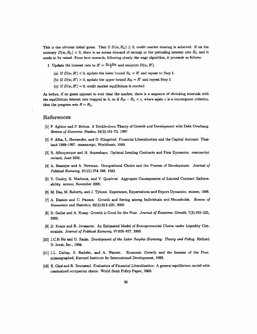
This is the obvious initial guess. Then if D(w, RL) > 0, credit market clearing is achieved. If on the

contrary D(w, RL) < 0, there is an excess demand of savings at the prevailing interest rate RL and it

needs to be raised. From here onwards, following closely the wage algorithm, it proceeds as follows:

1. Update the interest rate to R' = R,+RH and compute D(w, R').2

(a) If D(w, R') < 0, update the lower bound RL = R' and repeat to Step 1.

(b) If D(w, R') > 0, update the upper bound RH = R' and repeat Step 1.

(c) If D(w, R') = 0, credit market equilibrium is reached.

As before, if no guess appears to ever clear the market, there is a sequence of shrinking intervals with

the equilibrium interest rate trapped in it, so if RH - RL < e, where again e is a convergence criterion,

then the program sets R = RL.

References

[1] P. Aghion and P. Bolton. A Trickle-down Theory of Growth and Development wiht Debt Overhang.

Review of Economic Studies, 64(2):151-72, 1997.

[2] P. Alba, L. Hernandez, and D. Klingebiel. Financial Liberalization and the Capital Account: Thai-

land 1988-1997. manuscript, Worldbank, 1999.

[3] R. Albuquerque and H. Hopenhayn. Optimal Lending Contracts and Firm Dynamics. manuscript

revised, June 2001.

[4] A. Banerjee and A. Newman. Occupational Choice and the Process of Development. Journal of

Polstical Economy, 101(2):274-298, 1993.

[5] T. Cooley, R. Marimon, and V. Quadrini. Aggregate Consequences of Limited Contract Enforce-

ability. mimeo, November 2000.

[6] M. Das, M. Roberts, and J. Tybout. Experience, Expectations and Export Dynamics. mimeo, 1998.

[7] A. Deaton and C. Paxson. Growth and Saving among Individuals and Households. Review of

Economics and Statistics, 82(2):212-225, 2000.

[8] D. Dollar and A. Kraay. Growth is Good for the Poor. Journal of Economic Growth, 7(3):195-225,

2002.

[9] D. Evans and B. Jovanovic. An Estimated Model of Entrepreneurial Choice under Liquidity Con-

straints. Journal of Political Economy, 97:808-827, 1989.

[10] J.C.H Fei and G. Ranis. Development of the Labor Surplus Economy: Theory and Policy. Richard

D. Irwin, Inc., 1964.

[11] J.L. Gallup, S. Radelet, and A. Warner. Economic Growth and the Income of the Poor.

mimeographed, Harvard Institute for International Development, 1998.

[12] X. Gine and R. Townsend. Evaluation of Financial Liberalization: A general equilibrium model with

constrained occupation choice. World Bank Policy Paper, 2003.

36

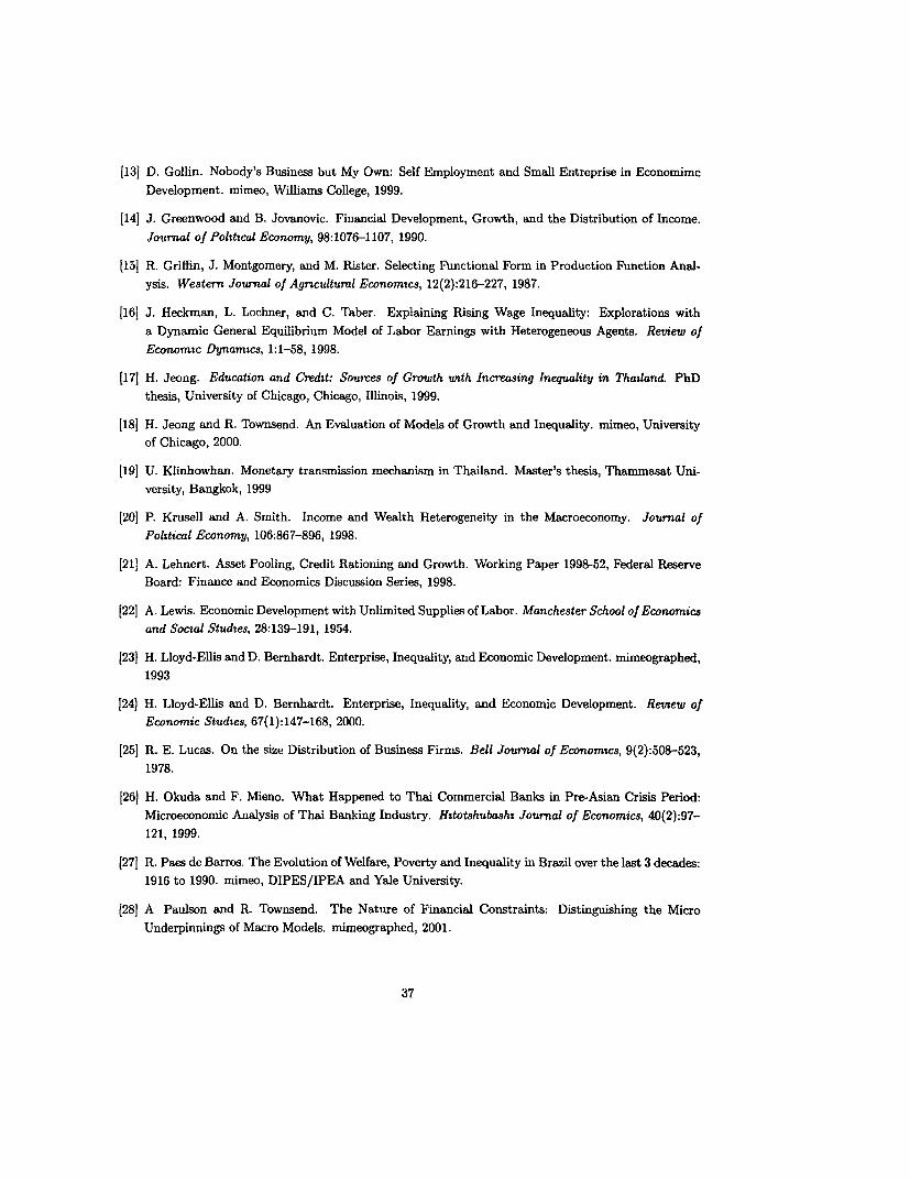
[131 D. Gollin. Nobody's Business but My Own: Self Employment and Small Entreprise in Economimc

Development. mimeo, Williams College, 1999.

[14] J. Greenwood and B. Jovanovic. Financial Development, Growth, and the Distribution of Income.

Journal of Polittcal Economy, 98:1076-1107, 1990.

[151 R. Griffin, J. Montgomery, and M. Rister. Selecting Functional Form in Production Function Anal-

ysis. Western Journal of Agncultural Economtcs, 12(2):216-227, 1987.

[161 J. Heckman, L. Lochner, and C. Taber. Explaining Rising Wage Inequality: Explorations with

a Dynamic General Equilibrium Model of Labor Earnings with Heterogeneous Agents. Review of

Economsc Dynamtcs, 1:1-58, 1998.

[171 H. Jeong. Education and Credit: Sources of Growth unth Increasing Inequality in Thatland. PhD

thesis, University of Chicago, Chicago, Illinois, 1999.

[18] H. Jeong and R. Townsend. An Evaluation of Models of Growth and Inequality. mimeo, University

of Chicago, 2000.

[19] U. Klinhowhan. Monetary transmission mechanism in Thailand. Master's thesis, Thammasat Uni-

versity, Bangkok, 1999

(201 P. Krusell and A. Smith. Income and Wealth Heterogeneity in the Macroeconomy. Journal of

Polztical Economy, 106:867-896, 1998.

[211 A. Lehnert. Asset Pooling, Credit Rationing and Growth. Working Paper 1998-52, Federal Reserve

Board: Finance and Economics Discussion Series, 1998.

[22] A. Lewis. Economic Development with Unlimited Supplies of Labor. Manchester School of Economics

and Social Studies, 28:139-191, 1954.

[23] H. Lloyd-Ellis and D. Bernhardt. Enterprise, Inequality, and Economic Development. mimeographed,

1993

[24) H. Lloyd-Ellis and D. Bernhardt. Enterprise, Inequality, and Economic Development. Retnew of

Economic Studies, 67(1):147-168, 2000.

[25] R. E. Lucas. On the size Distribution of Business Firms. Bell Journal of Economics, 9(2):508-523,

1978.

[26] H. Okuda and F. Mieno. What Happened to Thai Commercial Banks in Pre-Asian Crisis Period:

Microeconomic Analysis of Thai Banking Industry. Httotshubashi Journal of Economics, 40(2):97-

121, 1999.

[271 R. Paes de Barros. The Evolution of Welfare, Poverty and Inequality in Brazil over the last 3 decades:

1916 to 1990. mimeo, DIPES/IPEA and Yale University.

[28] A Paulson and R. Townsend. The Nature of Financial Constraints: Distinguishing the Micro

Underpinnings of Macro Models. mimeographed, 2001.

37

[29] T. Piketty. The Dynamics of the Wealth Distribution and the Interest Rate with Credit Rationing.Review of Economic Studies, 64:173-189, 1997.

[30] M. Ravallion. Growth, Inequality and Poverty: Looking Beyond Averages. World Development,29(11):1803-1815, 2001.

[31] M. Ravallion. The Debate on Globalization, Poverty and Inequality: Why Measurement Matters.mimeographed, The World Bank, 2002.

[32] T. Paul Schultz. Diminishing Returns to Scale in Family Planning Expenditures: Thailand, 1976-81mimeographed, Yale University, 1997.

[33] B. W. Silverman. Density Estimation for Statistics and Data Analysis. Chapman and Hall, London,England, 1986.

[341 P. Tinakorn and C. Sussangkarn. Total Factor Productivity Growth in Thailand: 1980-1995. mimeo,Macroeconomic Policy Program, TDRI, 1998.

[351 R. Townsend and K. Ueda. Transitional Growth with Increasing Inequality and Financial Deepening.mimeo, University of Chicago, 2001.

[36] R. Townsend principal investigator with A. Paulson, S. Sakuntasathien, T. J. Lee, and M. Binford.Questionnaire design and data collection for NICHD grant "Risk, Insurance and the Family," andNSF grants. mimeo, 1997.

[37] M. Veracierto. Plant Level Irreversible Investment and Equilibrium Business Cycles. mimeographed,1998.

38

: Hf i / E~m

b b

Figure 1: Occupational Choice Map

1~~~~~~~~~~~~~~~~~~~~9

Figure 2: Occupational Choice Map: SES data (left) and Townsend-Thai data (right)

39

Income Growth Savings Rate15 I

0 810

£ 8

/ - .2~~~~~~06

2 *~~~~~~~~~~~~~~~040 ol-- … --- --

-5 01980 1985 1990 1995 1980 1985 1990 1995

Labor Share Fraction of EntrepreneursI0 04

08

06…-- 01

01

0 01980 1985 1990 1995 1980 1985 19901 1995

Ginu Coefficient

08-

i206

804u

02

01980 1985 399 1995

Figure 3: Benchmark Model: Best Overall Fit (SES Data) .Legend: -- That Economy, - Simulation.

40

Income Growth Savings Rate

Xe<2( - 10

1980 1985 1990 1995 1980 1985 1990 1995

Labor Share Fraction of Entrepreneurs

I . . .............. ...I

N~~~~~~~~~~~~~~~04 -_ _ _ _ _ O-_ _ __________-____

0 ~ ~ ~ ~ ~ ~~~~~~~~~~~0

0 ~~~~~~~~~~~~~~~~~~0

1980 1985 1990 1995 1980 1985 1990 1995

Gmni Coefficient

08

E 06

E _ _ _ - -- - - ----_

020

o0.2

1980 1985 1990 1995

Figure 4: Benchmnark Model: Best Growvth Rate (SES Data).Legend: - T - -Simu!atn.

41

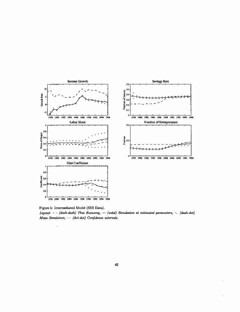
Income Growth Savings Rate

016geg r L _F_ ~~~~~~~~~~~~~~~~~~0°4 _..,-. ei

ol

1978 1980 1982 1984 1986 1988 1990 1992 1994 1996 1978 1980 1982 1984 1966 1988 1990 1992 1994 1996

Labor Share Fraction of Entrepreneurs

1978 980 182 184 196 198 s99 1992 1994 1996 1978 1980 1982 1984 1986 1988 1990 1992 1994 1996

Gini Coefficient

08

02'

1978 1980 1982 1984 1986 1988 1990 1992 1994 1996

Figure 5: Intermediated Model (SES Data).Legend: - - (dash-dash) Thai Economy, -(solid) Simulation at estimated parameters, -. (dash-dot)

Mean Simulation, *- (dot-dot) Confidence Cntervals.

42

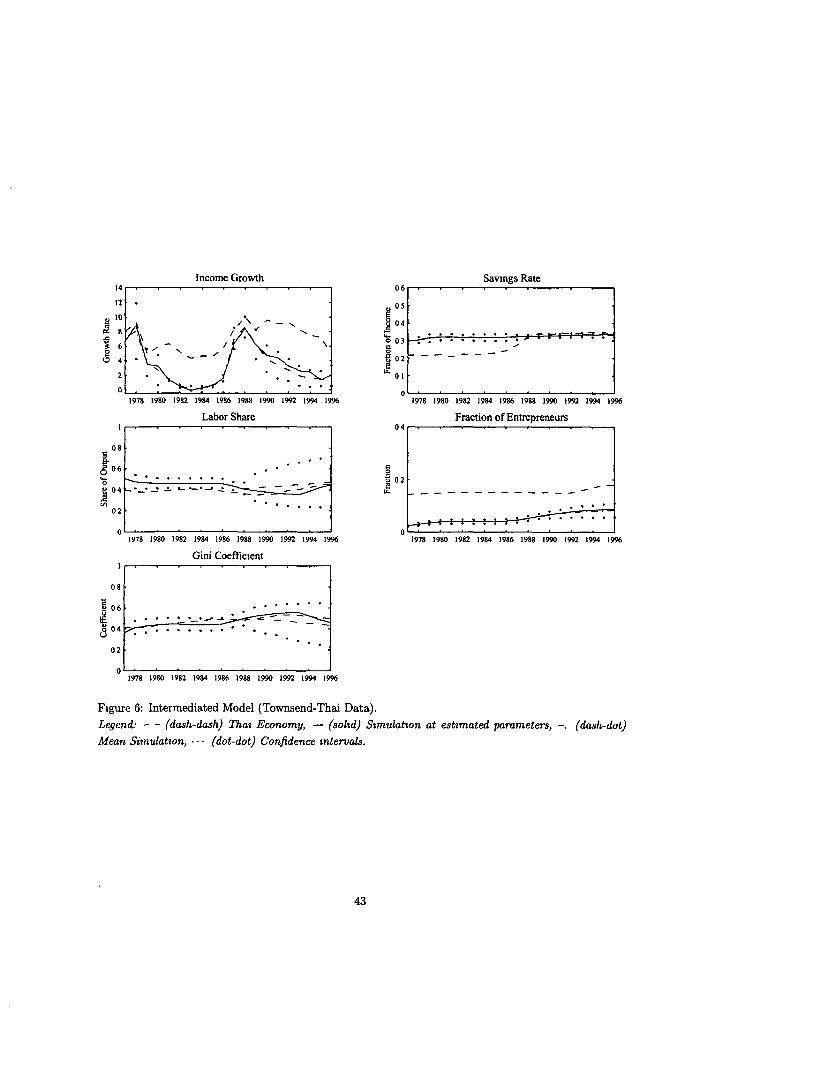
Income Growth Savings Rate142 0 6

014O 4 4 < ' _ cy oz~~~~~~0 . . . . . . . -

606 4 ' 02 .

1978 1980 1982 1984 1986 1988 1990 1992 1994 1996 1978 1980 1982 1984 1986 1988 1990 1992 1994 1996

Labor Share Fraction of Entrepreneurs

1978 1980 1982 1984 1986 1988 1990 199 1994 1996 1978 19S0 3982 3984 1986 1988 3990 3992 1994 1996

Gini Coefficient

43

08

_06 .*****-

804 -. - - - --

0 2

O .19818 9218 9618 9019 94161978 1980 1982 1984 1986 1988 1990 1992 1994 1996

Mean Simlatt Gini (dt-oefcnt) ofdnestra

0 4~ ~ ~~~~~~~4

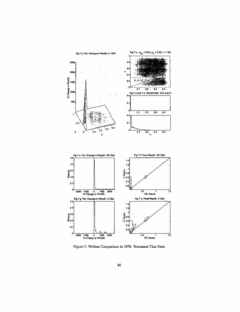
hg 7 a: Pc Change in Wealth m 1979 Flg7b. WNC=00

2.wC=OO2

,r8193

2500 08

06 z

2000 . x

0 1500 1 0

0.1 0.2 03 04IODO *oooF|ig 7 c and 7 d Wealth Dst' NCr and C

500 0.1

01 02 0.3 0.4

x 0 0.1 01 0.2 03 04b b

Fig 7 e Pd Change in Wealth NC Dist hg 7 f Final Wealth NC DIsL

1 4

0 04 12

0.2 O oe

0 4

01

-2000 -1000 0 1000 2000 05 1 15% Change in Wealth NC Sector

Figu7rg P Change InoWealthCDisL Fg 7 h. nal Weath C Dist

14

04 12,

4-0.3008

iE0.2 0 0.6

0.40.1

02

-2000 -1000 0 1000 2000 05 1 1.% Change in Wealth NC Sector

Figure 7: Welfare Comparison in 1979: Townsend-Thai Data

44

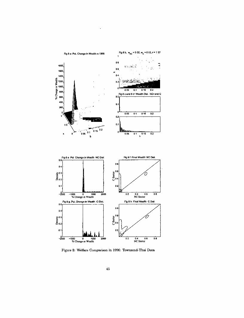
Fig 8 a: Pct Change in Wealth in 1996 Flg 8 b. WNC = 0 02, wC =° 03. r 1 571

08 - -:

1800 0 Wi Nt .-'.

0 6

1400 0 4 -

]1200 0 2 : - 'ff

g1000co O~~~~~~~~~~~~~~~~ 05 0.1 0 15 0 2

Fg 8 c and 8 d- Wealth Dist NCr and C

600J 1 s

0.10, _ 0 05 0 1 0 15 0.2

0221~~~~~~~~0 0 11 02 x 0 0105 0 05 01 015 02

b b

Fig 8 e Pct Change in Wealth NC Dilst Fig 8 f Final Wealth, NC Dist.

0.5~~~~~~~~~0

0 4

0.6->'0 3

0.1 02

-2000 -1000 0 1000O 2000 02 04 06 08% Change in Wealth NC Sector

Fig 8g.PcL WC elfane atth Coist Figi8h :nalnWea-Th Dist

080 4

f0 3 ~0 6

~~~~~0,2 ~ ~ ~ ~ ~ ~ ~~~~

01 0

-2000 -1000 0 1000 2000 0 2 0 4 0 6 0 8% Change in Wealth NC Sector

Figure 8: Welfare Comparison in 1996: Townsend-Thai Data

45

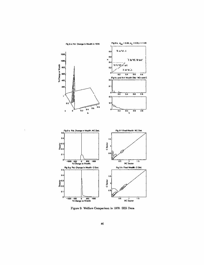
Flg9a:Pct ChangeinWeatthin 1978 Fig9b, WC=0.05.wc=005,r=149

0.812000

0.6

1000K0.4 -

Ma O 0.2

w 600 02 OA 0 6 08

Fig 9 c and 9 d Wealtt Dist NCr and CS400 02

200 01

0 2 OA 0.6 0 61 0°'

05 0.1

0 4 06 0x 0 0.2 02 04 06 08

b b

Fig 9 e Pct Change m Wealh. NC Dst. Fig 9 e Final Wealth NC Dlst.

0 4 1 5

Z'03

02 u

0 1 05

0-1000 -500 0 500 1000 0 5 1 1 5

% Change in Wealth NC Sector

Fig 9 g Pct. Change In Wealfth C Dtst. Fig 9 h Flnal Wealfth. C Dbst

041

02

0 1 0 5

-1000 -500 0 500 1000 05 1 15% Change in Wcalth NC Sector

Figure 9: Welfare Comparison in 1978: SES Data

46

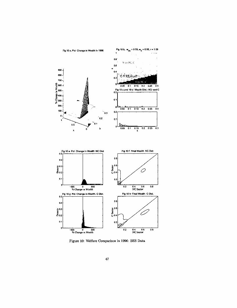
Fig O a. Pct Change In Wealth In 1996 Fig 10 b. wNc = 05, wc 0.08, r 1 09

0.8- \\ in N'(. C

0.6

9000

02700 0L j

sm_ 0 005 01 015 02 0.25 03

J30 Fig 10 c and 10 d Wealth Dist.: NCr and C

4 0 0 _

1300 9 | 03 0.1 ° ' 0 02 200,~ ~ ~ ~ ~~0

O 01

0.05 01 015 02 025 03

Fi 100a Pct Change In Wealth NC Dial Fig 10 f Final Wealth NC Distoot

B-0 3 °004

0.2 ~ ~ ~ 601 0.2

-50 0 50 020 041 062 0.850

Fig 109e Pct ChangeIn Wealth. C Dist Fig lOhf Final Wealth NCDist

0 5~ ~ ~~~~~~~0

i-0 3 ~~~~~~~08

IN0.2 c.U04

0 1 0.2

0 ---- 500 0 500 0 2 0 4 0 6 0.8% Change mn Wealth NC Secor

Fig0gurLChne 10: Weafare Comparison in 1996: Sina Deafta Ds

0.4 ~ ~ ~ ~ ~~4

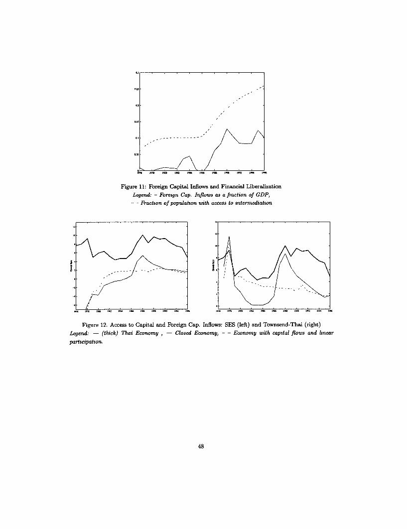
o ------- X---/-a

01

I j I9 W 1o 9:z im jm i li Ito I9 ti l9

Figure 11: Foreign Capital Inflows and Financial LiberalizationLegend: - Fomgn Cap. Inflows as a fraction of GDP,

- - Fraction of population with access to intermediatton

Figure 12. Access to Capital and Foreign Cap. Inflows: SES (left) and Townsend-Thai (right)

Legend: - (thick) Thai Economy, - Closed Economy, - - Economy with capital flows and linear

participation.

48

Policy Research Working Paper Series

ContactTitle Author Date for paper

WPS2996 Bank Competition, Financing Thorsten Beck March 2003 K LabrieObstacles, and Access to Credit Aslh Demirguc-Kunt 31001

Vojislav Maksimovic

WPS2997 Financial and Legal Institutions Thorsten Beck March 2003 K Labrieand Firm Size Asl1 Demirguq-Kunt 31001

Vojislav Maksimovic

WPS2998 Does Micro-Credit Empower Women? Mark M. Pitt March 2003 P KokilaEvidence from Bangladesh Shahidur R Khandker 31001

Jennifer Cartwright

WPS2999 Explaining Liberalization Philipp Harms March 2003 P FlewittCommitments in Financial Aaditya Mattoo 32724Services Trade Ludger Schuknecht

WPS3000 International Climate Regime beyond Franck Lecocq March 2003 V. Soukhanov2012 Are Quota Allocations Rules Renaud Crassous 35721Robust to Uncertainty?

WPS3001 An Introduction to Financial and Antonio Estache March 2003 G. Chenet-SmithEconomic Modeling for Utility Martin Rodriguez Pardina 36370Regulators Jose Maria Rodrfguez

German Sember

WPS3002 Information-Based Instruments for Uwe Deichmann March 2003 Y D'SouzaImproved Urban Management Somik V Lall 31449

Ajay SunPragya Rajoria

WPS3003 The Investment Climate and the Mary Hallward-Driemeier March 2003 P Sintim-AboagyeFirm Firm-Level Evidence from China Scott Wallsten 37644

Lixin Colhn Xu

WPS3004 Institutions, Trade, and Growth David Dollar March 2003 A. BonfieldRevisiting the Evidence Aart Kraay 31248

WPS3005 Vouchers for Basic Education in Varun Gauri March 2003 H. SladovichDeveloping Countries. A Principal- Ayesha Vawda 37698Agent Perspective

WPS3006 Social Rights and Economics Claims Varun Gauri March 2003 H Sladovichto Health Care and Education in 37698Developing Countries

WPS3007 The Impact of Urban Spatial Structure Antonio M Bento March 2003 V Soukhanovon Travel Demand in the United Maureen L. Cropper 35721States Ahmed Mushfiq Mobarak

Katja Vinha

WPS3008 Technology, Computers, and Wages Chris N. Sakellariou March 2003 N. VergaraEvidence from a Developing Economy Harry A. Patrinos 30432

WPS3009 Agriculture in the Doha Agenda Patrick Messerlin Apnl 2003 P. Flewitt32724

WPS3010 Vulnerability in Consumption, Edmundo Murrugarra April 2003 E MurrugarraEducation, and health Evidence from Jose Signoret 34452Moldova during the Russian Crisis

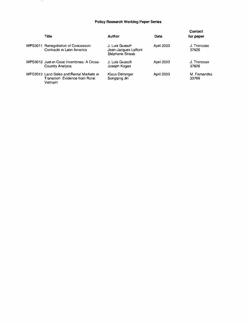
Policy Research Working Paper Series

ContactTitle Author Date for paper

WPS3011 Renegotiation of Concession J. Luis Guasch April 2003 J. TroncosoContracts in Latin America Jean-Jacques Laffont 37826

St6phane Straub

WPS3012 Just-in-Case Inventories: A Cross- J. Luis Guasch April 2003 J. TroncosoCountry Analysis Joseph Kogan 37826

WPS3013 Land Sales and Rental Markets in Klaus Deininger April 2003 M. FernandezTransition Evidence from Rural Songqing Jin 33766Vietnam