1

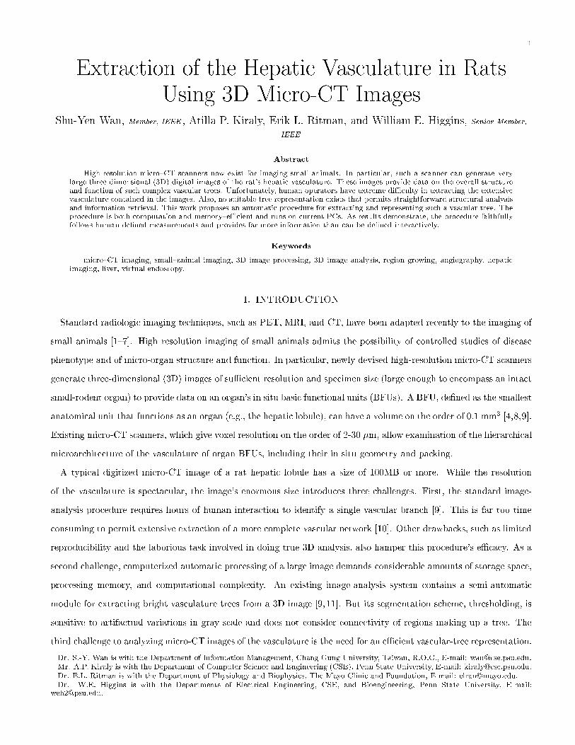
Extraction of the Hepatic Vasculature in RatsUsing 3D Micro-CT Images

Shu-Yen Wan, Member, IEEE , Atilla P. Kiraly, Erik L. Ritman, and William E. Higgins, Senior Member,

IEEE

Abstract

High-resolution micro{CT scanners now exist for imaging small animals. In particular, such a scanner can generate verylarge three-dimensional (3D) digital images of the rat's hepatic vasculature. These images provide data on the overall structureand function of such complex vascular trees. Unfortunately, human operators have extreme diÆculty in extracting the extensivevasculature contained in the images. Also, no suitable tree representation exists that permits straightforward structural analysisand information retrieval. This work proposes an automatic procedure for extracting and representing such a vascular tree. Theprocedure is both computation and memory{eÆcient and runs on current PCs. As results demonstrate, the procedure faithfullyfollows human-de�ned measurements and provides far more information than can be de�ned interactively.

Keywords

micro{CT imaging, small{animal imaging, 3D image processing, 3D image analysis, region growing, angiography, hepaticimaging, liver, virtual endoscopy.

I. INTRODUCTION

Standard radiologic imaging techniques, such as PET, MRI, and CT, have been adapted recently to the imaging of

small animals [1{7]. High resolution imaging of small animals admits the possibility of controlled studies of disease

phenotype and of micro-organ structure and function. In particular, newly devised high-resolution micro-CT scanners

generate three-dimensional (3D) images of suÆcient resolution and specimen size (large enough to encompass an intact

small-rodent organ) to provide data on an organ's in situ basic functional units (BFUs). A BFU, de�ned as the smallest

anatomical unit that functions as an organ (e.g., the hepatic lobule), can have a volume on the order of 0.1 mm3 [4,8,9].

Existing micro-CT scanners, which give voxel resolution on the order of 2-30 �m, allow examination of the hierarchical

microarchitecture of the vasculature of organ BFUs, including their in situ geometry and packing.

A typical digitized micro-CT image of a rat hepatic lobule has a size of 100MB or more. While the resolution

of the vasculature is spectacular, the image's enormous size introduces three challenges. First, the standard image-

analysis procedure requires hours of human interaction to identify a single vascular branch [9]. This is far too time

consuming to permit extensive extraction of a more complete vascular network [10]. Other drawbacks, such as limited

reproducibility and the laborious task involved in doing true 3D analysis, also hamper this procedure's eÆcacy. As a

second challenge, computerized automatic processing of a large image demands considerable amounts of storage space,

processing memory, and computational complexity. An existing image-analysis system contains a semi-automatic

module for extracting bright vasculature trees from a 3D image [9, 11]. But its segmentation scheme, thresholding, is

sensitive to artifactual variations in gray scale and does not consider connectivity of regions making up a tree. The

third challenge to analyzing micro-CT images of the vasculature is the need for an eÆcient vascular-tree representation.

Dr. S.-Y. Wan is with the Department of Information Management, Chang Gung University, Taiwan, R.O.C., E-mail: wan@cse.psu.edu.Mr. A.P. Kiraly is with the Department of Computer Science and Engineering (CSE), Penn State University, E-mail: kiraly@cse.psu.edu.Dr. E.L. Ritman is with the Department of Physiology and Biophysics, The Mayo Clinic and Foundation, E-mail: elran@mayo.edu.Dr. W.E. Higgins is with the Departments of Electrical Engineering, CSE, and Bioengineering, Penn State University, E-mail:

weh2@psu.edu.

2

Such a representation is necessary for eÆcient retrieval and analysis of a tree's structure, and it assists in visualization.

To address these challenges, we propose an eÆcient procedure for extracting and representing the vasculature of

the hepatic vascular system contained in micro{CT images. The procedure, inspired by a recently proposed system

for 3D angiographic analysis [12], is largely automatic and gives reproducible results. It employs a new 3D region

growing technique that is fast, memory{eÆcient, and relatively insensitive to starting conditions [13, 14]. The region

growing technique is also used for eÆcient deletion of interior cavities of the vascular network. Further, the complete

procedure employs a compact tree-representation scheme that permits rapid branch pruning, network reorganization,

and information retrieval. Section II of this paper describes the experimental protocol used in our e�orts. Section III

presents the proposed procedure. Section IV presents validation results for several micro-CT images of the blood

supply of rat hepatic lobes. Finally, Section V o�ers concluding remarks.

II. EXPERIMENTAL PROTOCOL

The rat was anesthetised and the ascending aorta exposed after a thoracotomy. After intravenous injection of

heparin, the rat was euthanised with an intravenous injection of pentobarbital. Next, the aorta was cannulated and

ushed with saline, following which micro�l (containing lead chromate) was infused at 100 mm Hg until it appeared

in the right ventricle. The aorta was ligated, and the animal placed in refrigerator overnight to permit the micro�l to

set. The next morning, the liver was removed and dehydrated with a sequence of immersions in glycerol of increasing

concentrations. Following this, the liver was �xed in bioplastic.

Next, the specimen was placed on top of a computer{controlled rotation stage in the micro-CT scanner. The scanner

is described in detail in [4]. In brief, it consists of a spectroscopy X{ray source that generates X{ray photons of a

nominal 18 keV energy. The X{rays transmitted through the specimen expose a crystalline plate of cesium iodide

(doped with thallium) which converts the X{ray image to a light image. This image is focused onto a CCD detector

array (1024�1024 square pixels, each 21 �m on a side) with a microscope objective operated at 1:1 or 1:4 magni�cation.

The specimen is rotated in 0.5 degrees around 360 degrees about its vertical axis in between each X{ray exposure. The

recorded X{ray projection gray scale was then converted to logarithmic values and a modi�ed Feldkamp cone beam

tomographic reconstruction performed. The resulting 3D image has cubic voxels, with each voxel being 21 �m on a

side. Each voxel has 16 bits of gray scale information.

III. ANALYSIS PROCEDURE

A. Image Characteristics

Our goal is to extract the vascular tree of the hepatic system and provide a complete geometric description of the

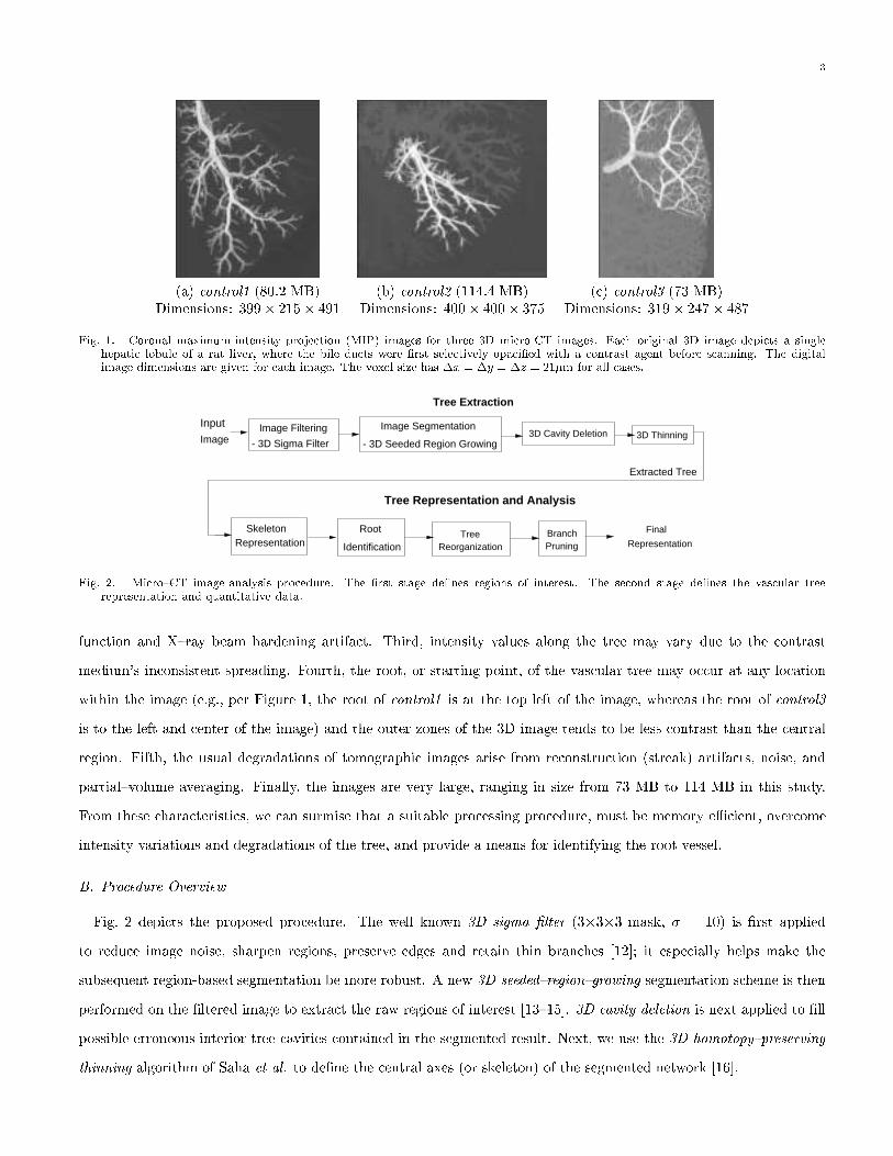
extracted tree. Fig. 1 shows 2D coronal (x{z) maximum{intensity projections (MIPs) for three of the 3D micro-CT

images used in this paper. Six characteristics are common to these images. First, the vascular tree appears brighter

than the background in the acquired images. Second, voxels at the middle of the larger proximal vessels may appear

dimmer than the other tree voxels. This occurs because of the fall-o� in the imaging system's modulation transfer

3

(a) control1 (80:2 MB) (b) control2 (114:4 MB) (c) control3 (73 MB)Dimensions: 399� 215� 491 Dimensions: 400� 400� 375 Dimensions: 319� 247� 487

Fig. 1. Coronal maximum-intensity projection (MIP) images for three 3D micro-CT images. Each original 3D image depicts a singlehepatic lobule of a rat liver, where the bile ducts were �rst selectively opaci�ed with a contrast agent before scanning. The digitalimage dimensions are given for each image. The voxel size has �x = �y = �z = 21�m for all cases.

- 3D Sigma Filter

Image Filtering

SkeletonRepresentation

- 3D Seeded Region Growing

Image Segmentation3D Cavity Deletion 3D Thinning

Root

Identification Reorganization Tree

PruningBranch

Image

Input

Tree Representation and Analysis

Extracted Tree

Tree Extraction

Representation

Final

Fig. 2. Micro{CT image-analysis procedure. The �rst stage de�nes regions of interest. The second stage de�nes the vascular treerepresentation and quantitative data.

function and X{ray beam hardening artifact. Third, intensity values along the tree may vary due to the contrast

medium's inconsistent spreading. Fourth, the root, or starting point, of the vascular tree may occur at any location

within the image (e.g., per Figure 1, the root of control1 is at the top left of the image, whereas the root of control3

is to the left and center of the image) and the outer zones of the 3D image tends to be less contrast than the central

region. Fifth, the usual degradations of tomographic images arise from reconstruction (streak) artifacts, noise, and

partial{volume averaging. Finally, the images are very large, ranging in size from 73 MB to 114 MB in this study.

From these characteristics, we can surmise that a suitable processing procedure, must be memory eÆcient, overcome

intensity variations and degradations of the tree, and provide a means for identifying the root vessel.

B. Procedure Overview

Fig. 2 depicts the proposed procedure. The well known 3D sigma �lter (3�3�3 mask, � = 10) is �rst applied

to reduce image noise, sharpen regions, preserve edges and retain thin branches [12]; it especially helps make the

subsequent region-based segmentation be more robust. A new 3D seeded{region{growing segmentation scheme is then

performed on the �ltered image to extract the raw regions of interest [13{15]. 3D cavity deletion is next applied to �ll

possible erroneous interior tree cavities contained in the segmented result. Next, we use the 3D homotopy{preserving

thinning algorithm of Saha et al. to de�ne the central axes (or skeleton) of the segmented network [16].

4

At this point, a complete thinned tree exists. This tree, however, demands excessive computer storage space,

especially considering that it typically contains >95% background voxels (0s). Further, it gives no information on

the tree's geometry or quantitative characteristics. Our proposed tree representation alleviates this burden. Four

steps are involved in building this representation: skeleton representation, to convert the raw 3D image of the skeleton

into a compact voxel list made up only of skeleton voxels; root identi�cation, to specify the tree's root branch; tree

reorganization, to reorder the tree's representation so that the identi�ed root branch starts the tree; and branch

pruning, to remove extraneous short branches. More details appear below on selected steps of the analysis procedure.

C. Procedure Details

Following ref. [12], let v denote the 3D image, (x; y; z) a voxel in the image, and v(x; y; z) the intensity of voxel

(x; y; z). The kth slice (or v(�; �; k)) of v refers to all voxels having coordinate z = k: wk is a working slice corresponding

to v(�; �; k) and wk(x; y) stores the temporary value of v(x; y; k). A foreground (background) voxel has value v(x; y; z) =

1 (0). A typical micro{CT image consists of an isotropically sampled Nx� Ny� Nz rectilinear lattice of voxels, where

the sampling intervals in each direction are equal: �x = �y = �z = �. This isotropy permits correct application of

true 3D digital image{processing operations [12].

An e�ective segmentation method must not only consider the image's intensity distribution, but also the spatial

relationships (connectivity) of voxels constituting the regions of interest. Our proposed region{growing algorithm takes

both factors into account and is a member of the class of symmetric region-growing algorithms [13,15]. The essential

property of a symmetric region-growing algorithm is that it will give the same segmented regions, regardless of which

points in the desired segmentation are used to start it. This property gives added robustness to di�erent initial growing

conditions.

The algorithm involves two main steps: (1) 2D region growing on the individual slices and (2) region merging

between consecutive slices to form complete regions. This approach enables one{pass processing. For each 2D slice,

the method starts with a set of seeds that meet certain restrictive criteria. These seeded regions then grow recursively

by including neighbors that satisfy loosened criteria until no further neighbors ar added. A 3D region, however, can

have any shape and grow in any direction. Thus, two issues must be addressed during growing and merging. First,

how should regions on consecutive slices be merged? And, second, how do regions on lower slices merge with \long

past" regions on upper slices?

To solve the �rst issue, the method employs a region table and an equivalence table [17]. The region table stores the

information on individual grown regions. This includes for each region: a region ID, dimensions of its bounding{box,

number of seeds, and number of pixels (in 2D respect), acquired from 2D seeded region growing on each slice. The

equivalence table contains composite information on 3D regions after merging. Each entry of the equivalence table

maintains a list of region IDs of equivalent regions and other accumulated data obtained from the region table. Each

entry of the region table also has a pointer linked to its corresponding entry in the equivalence table. At the end of

the growing and merging process, the equivalence table is taken as the �nal region table.

5

The answer to the second issue is more complex. As the growing and merging processes progress, a (2D) region

in the region table could be considered as interesting or pending, while the (3D) region in the equivalence table can

be considered as active, inactive, deletable, or desired. When the growing process �nishes on the �rst slice (k = 0), a

2D region can be categorized as: (1) an interesting region that contains seeds; (2) a pending region that contains no

seeds but whose voxels satisfy loosened restrictions; (3) a background region that contains the remaining voxels. The

background regions are neglected, while the information of the interesting and pending regions are stored in the region

table. The merging process starts on slice k when region information becomes available on slice (k � 1) above it. A

3D region (in the equivalence table) is further labeled as active if it is involved in the merging process on the current

slice or as inactive otherwise. The inactive 3D regions are evaluated according to other speci�cations: (1) minimum

number of seeds in the region and (2) minimum required number of voxels in the region. After the evaluation, the

inactive regions are then marked as desired, if they pass the speci�cations, or deletable otherwise. After the last

slice (k = Nz � 1) is visited, every region is marked as either desired or deletable. Only the desired regions are kept

as the �nal 3D regions.

Since the processing of a 3D image only requires one pass through the 2D slices, the visited slices are no longer used

and the voxels on them can store their region numbers. Therefore, 3D seeded region growing requires only one copy

of the image, plus a small amount of working bu�er to maintain the region and equivalence tables. Since the main

mechanism works in 2D, previously developed 2D methods can be exploited and adapted to our framework [18, 19].

A voxel looks for at most 8 neighbors for growing, instead of 26 if done in 3D. The reduction of computation time is

signi�cant, especially for huge images. When merging takes place, the overlapping (in x{ and y{coordinates) portions

of active regions on consecutive (k and (k � 1)) slices are checked. Complete detail on the method appears below.

In the following description, NumOfSeeds(Ri) gets the number of seeds in Ri. NumOfVoxels(Ri) gets the number

of voxels in Ri. NumOfRegions denotes the number of regions. Before processing, the user prede�nes the criteria for

acceptable ROIs and how to grow the regions: GseedMin , GseedMax, Gmin, Gmax, Gtolerance, Gconnectivity , GleastSeeds ,

GminSize. [GseedMin ,GseedMax] speci�es the intensity range for valid seeds. [Gmin,Gmax] determines the allowed

intensity for voxels in the �nal regions { no voxel outside this range will be in the �nal regions. Therefore, Gmin �

GseedMin � GseedMax � Gmax. A voxel that is not a seed is added to an existing region if the intensity di�erence

between it and any of its neighbors in the region is less than or equal to Gtolerance. Gconnectivity speci�es the search{

neighborhood sizes during growing. Please note that although Gconnectivity is speci�ed as 26 or 6, in 3D respect, during

2D region growing, 26 is interpreted as 8 and 6 as 4, in 2D respect. The user speci�es the minimum number of seeds

and voxels a valid region must have using the parameters GleastSeeds and GminSize. The complete algorithm appears

below. Part 1 summarizes the top{level method. Parts 2 and 3 describe the lower{level stages.

1. 3D Seeded Region Growing

For slice k = 0 to Nz � 1.

Perform 2D Seeded Region Growing on slice k

6

If k � 1 Do Region Merging for slices k and (k � 1)

For all voxels (x; y; z), v(x; y; z) = 1 if the region it belongs to is desired; otherwise, v(x; y; z) = 0.

2. 2D Seeded Region Growing on slice k

(a) Initialization: Begin with voxel (0; 0; 0).

(b) Find the next voxel (x; y; k) such that Gmin � v(x; y; k) � Gmax. Assign the next available region number to

(x; y; k); i.e., wk(x; y) NumOfRegions. NumOfRegions= NumOfRegions+1.

(c) Examine (x; y; k)'s Gconnectivity neighbors. Include the neighbor (x0; y0; k) recursively in a region if and only if

the following predicate is TRUE:

(P1 AND ((P0 AND (P2 OR (P3 AND P4))) OR (P0 AND (P3 AND P4))))

P0 = fv(x; y; k) in [GseedMin; GseedMax]g { (x; y; k) is a valid seed.

P0 = fv(x; y; k) not in [GseedMin; GseedMax]g { (x; y; k) is not a valid seed.

P1 = fwk(x0; y0) unde�nedg { (x0; y0; k) has not been been visited yet.

P2 = fv(x0; y0; k) in [GseedMin; GseedMax]g { The neighbor v(x0; y0; k) is a valid seed.

P3 = fv(x0; y0; k) in [Gmin; Gmax]g { The neighbor v(x0; y0; k) is in the allowed intensity range.

P4 = fjv(x; y; k)� v(x0; y0; k)j � Gtoleranceg { v(x0; y0; k) is close enough to v(x; y; k) to be added to a region.

(d) Go to 2b if more voxels on slice k still need to be examined. If not, write the values of wk back to slice v(�; �; k):

v(x; y; k) wk(x; y), 8x; y.

(e) Generate the following 2D region information: region ID, dimensions of the region's 2D bounding box on slice

k, number of seeds, and number of voxels. The regions containing zero seeds are labeled as pending ; otherwise,

they are labeled as interesting.

3. Region Merging for slice k and (k � 1)

(a) Locate all overlapping portions of the active regions between the current (kth) slice and the previous ((k�1)th)

slice . A region's bounding box is used to check for overlap.

(b) Examine whether overlapping active regions should be merged. Within the overlapping portion for voxel

(x; y; k) on the current slice, check its upper 5 or 9 neighbors on slice (k � 1), according to Gconnectivity . (5

neighbors: center voxel and 4{neighbors; 9 neighbors: center voxel and 8{neighbors.) Two regions are merged

if and only if the following predicate is true:

((P0 AND (P1 OR P2)) OR (P0 AND P2))

P0 = fv(x; y; k) in [GseedMin; GseedMax]g { v(x; y; k) is a valid seed.

P0 = fv(x; y; k) not in [GseedMin; GseedMax]g { v(x; y; k) is not a valid seed.

P1 = fv(x0; y0; k) in [GseedMin; GseedMax]g { The neighbor v(x0; y0; k) is a valid seed.

P2 = fjv(x; y; k)� v(x0; y0; k)j � Gtoleranceg { v(x0; y0; k) is close enough to v(x; y; k) to be added to a region.

7

(c) Update the equivalence table so that the region IDs of the merged regions are listed in the same equivalence

entry. Go to 3b until all overlapping active regions have been checked.

(d) A 3D region (in the equivalence table) is labeled as active if it is involved in the merging process; otherwise,

it is labeled as inactive.

(e) Evaluate 3D regions. Mark a region as deletable if NumOfSeeds(Ri) < GleastSeeds or NumOfVoxels(Ri) <

GminSize. Otherwise, mark the region as desired.

Region seeds correspond to bright voxels above a prespeci�ed intensity value (GseedMin) that form reasonably large

(GleastSeeds) connected clusters. Voxels added to the tree during growing must be locally homogeneous relative to

voxels already contained in the tree (within Gtolerance) and must lie above a prespeci�ed minimum intensity value

(Gmin). When the algorithm ends, the �nal outputs are: (1) an image where each voxel stores the ID of its member

region; (2) a region table that contains information on all 3D regions, including whether a region is desired (set to 1)

or part of the background (set to 0).

While region growing is robust, the inconsistent gray scale of the contrast medium may cause interior cavities to

exist in the grown tree. Such cavities should not exist and adversely alter the tree's digital topology. 3D cavity deletion

gives an extra precaution that makes the overall micro-CT analysis procedure less sensitive to scanning irregularities.

The cavity deletion process performs 3D connected-component labeling on the \0" voxels; this is adapted from our 3D

seeded region{growing algorithm [13, 15]. The components not adjacent to the image's outer boundary are cavities.

These are �lled with \1" voxels, giving a result containing a simply-connected vascular tree.

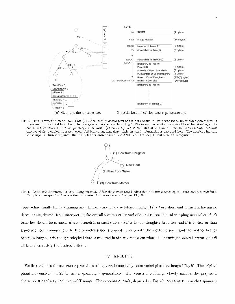
The proposed tree representation stores the skeleton of the vascular tree in a compact lossless form. It permits

complete reconstruction of the original thinned image for later display. Also, it provides considerable information

on the tree's structure. Our implementation traverses the skeleton image and dynamically establishes the tree{

like branching structure as shown in Fig. 3a. The structure permits straightforward de�nitions of topological and

geometrical information. It is similar to the symbolic graph-like description suggested for the cerebral vasculature by

Szekely et al. [20].

No prior knowledge of the tree's root (generation #0) branch has yet been used to this point: the skeleton represen-

tation takes the �rst encountered end voxel as the root. As discussed earlier, Fig. 1a-b show that the �rst encountered

end voxel does not necessarily belong to the root. Therefore, the tree representation of Fig. 3a does not necessarily

indicate the correct branch relationships. We de�ne the tree's root interactively. For interactive de�nition, the user

can invoke a 3D visualization system to manually identify a root location. The tree's end voxel closest to the manu-

ally input 3D coordinates are then assigned as the root. Once the root is determined, the previously computed tree

hierarchy undergoes a reorganization, as shown in Fig. 4. As this point, anatomically correct tree information, such

as mother{daughter relationships and generation numbers (tree levels) are computed. Fig. 3b shows the data format

for the representation.

The tree representation gives a means for straightforward computationally eÆcient branch pruning. (Other pruning

8

#0

#1#2

#3#4

ppBranchH

pParent

ppSister

GenID = 2

#Sisters = 1ppDaughter = NULL

TreeID = 0BranchID = 3

SKMM (4 bytes)

(348 bytes)

Number of Trees T (2 bytes)

BYTE

#Branches in Tree(0)

#Branches in Tree(T-1)

(2 bytes)

(2 bytes)

Parent ID

Branch Voxel List

(2 bytes)(2 bytes)(2 bytes)

(2*D(0) bytes)(6*V(0) bytes)

::

Branch#N in Tree(T-1)

Branch#0 in Tree(0)

Branch#1 in Tree(0)

::::

:

354

352-253

4-351

0-3

353+2*T+6*2D(0)+6V(0)

353+2*T+1

353+2*T

Branch IDs of Daughters

#Voxels V(0) on Branch#0#Daughters D(0) of Branch#0

Image Header

(a) Skeleton data structure. (b) File format of the tree representation

Fig. 3. Tree representation scheme. Part (a) schematically shows part of the data structure for a tree made up of three generations ofbranches and �ve total branches. The �rst generation starts at branch #0. The second generation consists of branches starting at theend of branch #0, etc. Branch genealogy information (parent, etc.) is also compiled at this point. Part (b) shows a small exampleexcerpt of the complete representation. All branching, genealogy, skeleton-voxel information is captured here. The numbers indicatethe computer storage required (the image header data assumes the ANALYZE header [11], but this is not required).

(2) Flow from Sister

(3) Flow from Mother

New Root

(1) Flow from Daughter

Fig. 4. Schematic illustration of Tree Reorganization. After the correct root is identi�ed, the tree's genealogical organization is rede�ned.Complete tree speci�cations are then computed for the representation, per Fig. 3b.

approaches usually follow thinning and, hence, work on a voxel{based image [12].) Very short end branches, having no

descendants, detract from interpreting the overall tree structure and often arise from digital sampling anomalies. Such

branches should be pruned. A tree branch is pruned (deleted) if it has no daughter branches and if it is shorter than

a prespeci�ed minimum length. If a branch's sister is pruned, it joins with the mother branch, and the mother branch

becomes longer. A�ected genealogical data is updated in the tree representation. The pruning process is iterated until

all branches satisfy the desired criteria.

IV. RESULTS

We �rst validate the automatic procedure using a mathematically constructed phantom image (Fig. 5). The original

phantom consisted of 23 branches spanning 8 generations. The constructed image closely mimics the gray-scale

characteristics of a typical micro-CT image. The automatic result, depicted in Fig. 5b, contains 19 branches spanning

9

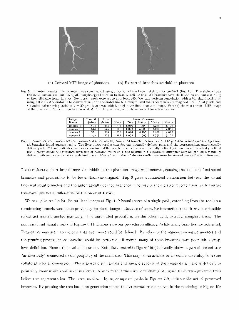
(a) Coronal MIP image of phantom (b) Extracted branches overlaid on phantom

Fig. 5. Phantom results. The phantom was constructed using a portion of the known skeleton for control1 (Fig. 1b). This skeleton wasthickened various amounts using 3D morphological dilation to form a realistic tree. All branches were thickened an amount accordingto their distance from the root. Next, tree voxels were set to gray level 200. We then perform convolution with a blurring function byusing a 3� 3� 3 operator. The central voxel of the operator has 60% weight, and the other voxels are weighted 40%. Finally, additiveGaussian noise having variance � = 20 gray levels was added, to give the �nal phantom image. Part (a) shows a coronal MIP imageof the phantom. Part (b) depicts a coronal MIP of the phantom, with the extracted branches overlaid.

Image Manual Auto Error MeasuresName #sites #sites Mean Dev Max x Max y Max z

phantom 514 495 1.013 1.010 1.500 1.200 1.100

control1 544 525 1.888 1.676 5.000 3.000 12.330

control2 271 298 1.592 1.014 5.750 2.900 4.080

control3 252 225 3.481 1.903 4.090 4.730 6.420

Fig. 6. Numerical comparison between known and automatically computed branch measurements. The phantom results give averages overall branches found automatically. The liver-image results consider one manually de�ned path and the corresponding automaticallyde�ned path. \Mean" indicates the mean coordinate di�erence between sites on an manually de�ned path and an automatically de�nedpath. \Dev" equals the standard deviation of \Mean." \Max x" is the maximum x{coordinate di�erence over all sites on a manuallyde�ned path and an automatically de�ned path. \Max y" and \Max z" denote similar measures for y{ and z{coordinate di�erences.

7 generations; a short branch near the middle of the phantom image was removed, causing the number of extracted

branches and generations to be fewer than the original. Fig. 6 gives a numerical comparison between the actual

known skeletal branches and the automatically de�ned branches. The results show a strong correlation, with average

tree-voxel positional di�erences on the order of 1 voxel.

We next give results for the rat liver images of Fig. 1. Manual traces of a single path, extending from the root to a

terminating branch, were done previously for these images. Because of excessive interaction time, it was not feasible

to extract more branches manually. The automated procedure, on the other hand, extracts complete trees. The

numerical and visual results of Figures 6-11 demonstrate our procedure's eÆcacy. While many branches are extracted,

Figures 7-9 may seem to indicate that even more could be de�ned. By relaxing the region-growing parameters and

the pruning process, more branches could be extracted. However, many of these branches have poor initial gray-

level de�nition. Hence, their value is unclear. Note that control3 (Figure 10(c)) actually shows a partial second tree

\artifactually" connected to the periphery of the main tree. This may be an artifact or it could conceivably be a true

collateral arterial connection. The gray-scale similarities and sample spacing of the image data make it diÆcult to

positively know which conclusion is correct. Also note that the surface rendering of Figure 10 shows segmented trees

before tree representation. The trees, as shown by superimposed paths in Figures 7-9, indicate the actual preserved

branches. By pruning the tree based on generation index, the artifactual tree depicted in the rendering of Figure 10c

10

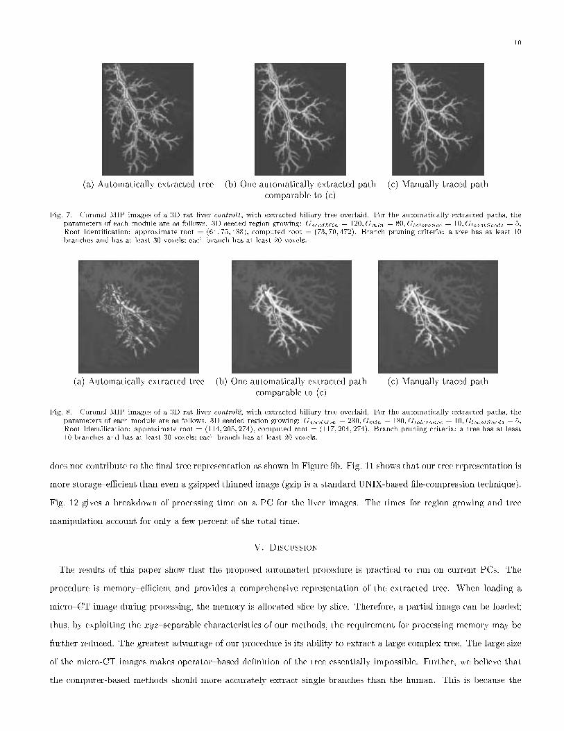
(a) Automatically extracted tree (b) One automatically extracted path (c) Manually traced pathcomparable to (c)

Fig. 7. Coronal MIP images of a 3D rat liver control1, with extracted biliary tree overlaid. For the automatically extracted paths, theparameters of each module are as follows. 3D seeded region growing: GseedMin = 120; Gmin = 80;Gtolerance = 10; GleastSeeds = 5,Root Identi�cation: approximate root = (64; 75; 488), computed root = (73; 70; 472). Branch pruning criteria: a tree has at least 10branches and has at least 30 voxels; each branch has at least 20 voxels.

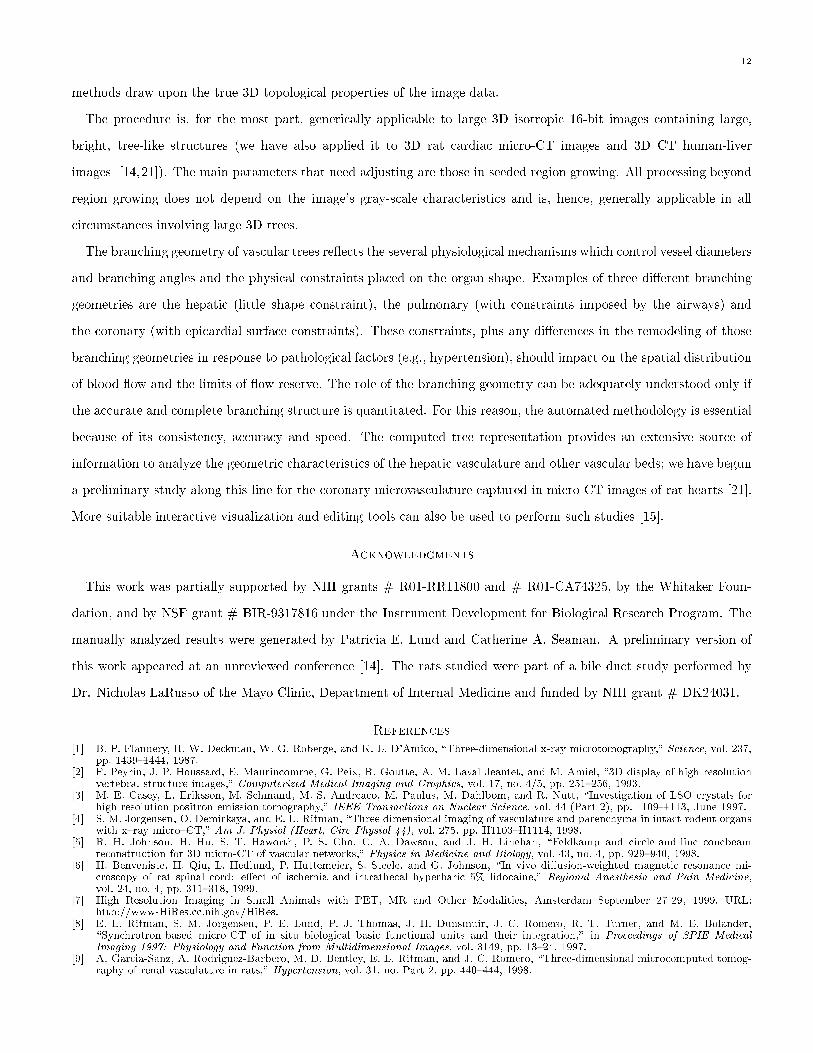
(a) Automatically extracted tree (b) One automatically extracted path (c) Manually traced pathcomparable to (c)

Fig. 8. Coronal MIP images of a 3D rat liver control2, with extracted biliary tree overlaid. For the automatically extracted paths, theparameters of each module are as follows. 3D seeded region growing: GseedMin = 230; Gmin = 180; Gtolerance = 10; GleastSeeds = 5,Root Identi�cation: approximate root = (114; 205; 274), computed root = (117; 204; 274). Branch pruning criteria: a tree has at least10 branches and has at least 30 voxels; each branch has at least 20 voxels.

does not contribute to the �nal tree representation as shown in Figure 9b. Fig. 11 shows that our tree representation is

more storage{eÆcient than even a gzipped thinned image (gzip is a standard UNIX-based �le-compression technique).

Fig. 12 gives a breakdown of processing time on a PC for the liver images. The times for region growing and tree

manipulation account for only a few percent of the total time.

V. Discussion

The results of this paper show that the proposed automated procedure is practical to run on current PCs. The

procedure is memory{eÆcient and provides a comprehensive representation of the extracted tree. When loading a

micro{CT image during processing, the memory is allocated slice by slice. Therefore, a partial image can be loaded;

thus, by exploiting the xyz{separable characteristics of our methods, the requirement for processing memory may be

further reduced. The greatest advantage of our procedure is its ability to extract a large complex tree. The large size

of the micro-CT images makes operator{based de�nition of the tree essentially impossible. Further, we believe that

the computer-based methods should more accurately extract single branches than the human. This is because the

11

(a) Auto-extracted tree (b) Pruned (a) by generation index (c) One path from (a) (d) Manually traced pathcomparable to (d)

Fig. 9. Coronal MIP images of 3D rat liver control3, with extracted biliary tree overlaid. For the automatically extracted paths, theparameters of each module are as follows. 3D seeded region growing: GseedMin = 200; Gmin = 130; Gtolerance = 10; GleastSeeds = 5,Root Identi�cation: approximate root = (13; 165; 292), computed root = (28; 92; 303). Branch pruning criteria: a tree has at least 10branches and has at least 30 voxels; each branch has at least 20 voxels. Reference [14] gives complete detail on the parameters.

(a) control1 (b) control2 (c) control3

Fig. 10. 3D surface renderings of extracted vascular trees.

Image Tree Data Storage RequirementsName #br #gen size thin gzip tree

control1 51 14 80.2MB 40.1MB 52KB 9KB

control2 15 6 114.4MB 57.2MB 65KB 13KB

control3 69 12 73.0MB 36.5MB 44KB 18KB

Fig. 11. Pro�le of automated results for the rat livers. #br and #gen denote numbers of branches and generations extracted by theautomatic procedure. The storage requirements indicate the how much storage a particular form uses; \size" denotes the original 3Dimage, \thin" denotes the image after 3D thinning, \gzip" is a gzipped version of the thinned image, and \tree" is our proposed treerepresentation.

Image Image Time usage (in seconds)Name Size sig seg cav thin rep man totalcontrol1 80.2MB 104 8 69 121 6 � 1 309

control2 114.4MB 147 9 98 6 8 � 1 269

control3 73.0MB 95 8 64 291 5 � 1 464

Fig. 12. Running time usage on a PC (Windows NT, CPU 400MHz). sig=fSigma Filterg; seg=f3D seeded region growingg; cav=fcavitydeletiong; thin=fthinningg; rep=fSkeleton representationg; man=fSkeleton manipulation: Root Identi�cation, Tree Reorganization,Pruning.g.

12

methods draw upon the true 3D topological properties of the image data.

The procedure is, for the most part, generically applicable to large 3D isotropic 16-bit images containing large,

bright, tree-like structures (we have also applied it to 3D rat cardiac micro-CT images and 3D CT human-liver

images [14,21]). The main parameters that need adjusting are those in seeded region growing. All processing beyond

region growing does not depend on the image's gray-scale characteristics and is, hence, generally applicable in all

circumstances involving large 3D trees.

The branching geometry of vascular trees re ects the several physiological mechanisms which control vessel diameters

and branching angles and the physical constraints placed on the organ shape. Examples of three di�erent branching

geometries are the hepatic (little shape constraint), the pulmonary (with constraints imposed by the airways) and

the coronary (with epicardial surface constraints). These constraints, plus any di�erences in the remodeling of those

branching geometries in response to pathological factors (e.g., hypertension), should impact on the spatial distribution

of blood ow and the limits of ow reserve. The role of the branching geometry can be adequately understood only if

the accurate and complete branching structure is quantitated. For this reason, the automated methodology is essential

because of its consistency, accuracy and speed. The computed tree representation provides an extensive source of

information to analyze the geometric characteristics of the hepatic vasculature and other vascular beds; we have begun

a preliminary study along this line for the coronary microvasculature captured in micro-CT images of rat hearts [21].

More suitable interactive visualization and editing tools can also be used to perform such studies [15].

Acknowledgments

This work was partially supported by NIH grants # R01-RR11800 and # R01-CA74325, by the Whitaker Foun-

dation, and by NSF grant # BIR-9317816 under the Instrument Development for Biological Research Program. The

manually analyzed results were generated by Patricia E. Lund and Catherine A. Seaman. A preliminary version of

this work appeared at an unreviewed conference [14]. The rats studied were part of a bile duct study performed by

Dr. Nicholas LaRusso of the Mayo Clinic, Department of Internal Medicine and funded by NIH grant # DK24031.

References

[1] B. P. Flannery, H. W. Deckman, W. G. Roberge, and K. L. D'Amico, \Three-dimensional x-ray microtomography," Science, vol. 237,pp. 1439{1444, 1987.

[2] F. Peyrin, J.-P. Houssard, E. Maurincomme, G. Peix, R. Goutte, A.-M. Laval-Jeantet, and M. Amiel, \3D display of high resolutionvertebral structure images," Computerized Medical Imaging and Graphics, vol. 17, no. 4/5, pp. 251{256, 1993.

[3] M. E. Casey, L. Eriksson, M. Schmand, M. S. Andreaco, M. Paulus, M. Dahlbom, and R. Nutt, \Investigation of LSO crystals forhigh resolution positron emission tomography," IEEE Transactions on Nuclear Science, vol. 44 (Part 2), pp. 1109{1113, June 1997.

[4] S. M. Jorgensen, O. Demirkaya, and E. L. Ritman, \Three dimensional imaging of vasculature and parenchyma in intact rodent organswith x{ray micro{CT," Am J. Physiol (Heart, Circ Physiol 44), vol. 275, pp. H1103{H1114, 1998.

[5] R. H. Johnson, H. Hu, S. T. Haworth, P. S. Cho, C. A. Dawson, and J. H. Linehan, \Feldkamp and circle-and-line conebeamreconstruction for 3D micro-CT of vascular networks," Physics in Medicine and Biology, vol. 43, no. 4, pp. 929{940, 1998.

[6] H. Benveniste, H. Qiu, L. Hedlund, P. Huttemeier, S. Steele, and G. Johnson, \In vivo di�usion-weighted magnetic resonance mi-croscopy of rat spinal cord: e�ect of ischemia and intrathecal hyperbaric 5% lidocaine," Regional Anesthesia and Pain Medicine,vol. 24, no. 4, pp. 311{318, 1999.

[7] High Resolution Imaging in Small Animals with PET, MR and Other Modalities, Amsterdam September 27-29, 1999. URL:http://www-HiRes.cc.nih.gov/HiRes.

[8] E. L. Ritman, S. M. Jorgensen, P. E. Lund, P. J. Thomas, J. H. Dunsmuir, J. C. Romero, R. T. Turner, and M. E. Bolander,\Synchrotron-based micro-CT of in situ biological basic functional units and their integration," in Proceedings of SPIE MedicalImaging 1997: Physiology and Function from Multidimensional Images, vol. 3149, pp. 13{24, 1997.

[9] A. Garcia-Sanz, A. Rodriguez-Barbero, M. D. Bentley, E. L. Ritman, and J. C. Romero, \Three-dimensional microcomputed tomog-raphy of renal vasculature in rats," Hypertension, vol. 31, no. Part 2, pp. 440{444, 1998.

13

[10] P. E. Lund, C. A. Seaman, and E. L. Ritman, \3D branching geometries of epicardial and intra-myocardial coronary arteries in 3 to25-week old rats," American Jounal of Physiology (Heart, Circulatory Physiology), In Review 1999.

[11] R. A. Robb, Three-Dimensional Biomedical Imaging: Principles and Practice. New York: VCH Publishers, 1994.[12] W. E. Higgins, R. A. Karwoski, W. J. T. Spyra, and E. L. Ritman, \System for analyzing true three-dimensional angiograms," IEEE

Transactions on Medical Imaging, vol. 15, pp. 377{385, June 1996.[13] S.-Y. Wan and W. Higgins, \Symmetric region growing," IEEE International Conference on Image Processing (ICIP2000), to appear

2000.[14] S.-Y. Wan, E. L. Ritman, and W. E. Higgins, \Extraction and analysis of large vascular networks in 3D micro-CT images," in

Proceedings of SPIE Medical Imaging 1999: Physiology and Function from Multidimensional Images, vol. 3660, pp. 322{334, A.Clough and C.T Chen, eds., 1999.

[15] S.-Y. Wan, \Analysis and visualization of large branching networks in 3-D digital images," Ph.D. Dissertation, Dept. ComputerScience and Engineering, The Pennsylvania State University, August 2000.

[16] P. K. Saha, B. B. Chaudhuri, and D. D. Majumder, \A new shape preserving parallel thinning algorithm for 3D digital images,"Pattern Recognition, vol. 30, no. 12, pp. 1939{1955, 1997.

[17] R. Jain, R. Kasturi, and B. G. Schunck, Machine Vision. New York: MIT Press and McGraw-Hill Inc., 1995.[18] R. M. Haralick and L. G. Shapiro, \Survey: Image segmentation techniques," Computer Vision, Graphics and Image Processing,

vol. 29, pp. 100{132, January 1985.[19] Y.-L. Chang and X. Li, \Adaptive image region-growing," IEEE Transactions on Image Processing, vol. 3, pp. 868{872, November

1994.[20] G. Szekely, T. Koller, R. Kikinis, and G. Gerig, \Structural description and combined 3-D display for superior analysis of cerebral

vascularity from MRA," in Proc. SPIE, vol. 2359, pp. 272{281, 1994.[21] S.-Y. Wan, P. E. Lund, D. A. Reyes, C. A. Seaman, W. E. Higgins, and E. L. Ritman, \Heterogeneity of coronary arterial branching

geometry," in Proceedings of SPIE Medical Imaging 2000: Physiology and Function from Multidimensional Images, vol. 3978, pp. 515{520, A. Clough and C.T Chen, eds., 2000.