Extended Analytical Charge Modeling for Permanent-Magnet ...

Extended analytical charge modeling for permanent-magnetbased devices : practical application to the interactions in avibration isolation systemCitation for published version (APA):Janssen, J. L. G. (2011). Extended analytical charge modeling for permanent-magnet based devices : practicalapplication to the interactions in a vibration isolation system. [Phd Thesis 1 (Research TU/e / Graduation TU/e),Electrical Engineering]. Technische Universiteit Eindhoven. https://doi.org/10.6100/IR719555

DOI:10.6100/IR719555

Document status and date:Published: 01/01/2011

Document Version:Publisher’s PDF, also known as Version of Record (includes final page, issue and volume numbers)

Please check the document version of this publication:

• A submitted manuscript is the version of the article upon submission and before peer-review. There can beimportant differences between the submitted version and the official published version of record. Peopleinterested in the research are advised to contact the author for the final version of the publication, or visit theDOI to the publisher's website.• The final author version and the galley proof are versions of the publication after peer review.• The final published version features the final layout of the paper including the volume, issue and pagenumbers.Link to publication

General rightsCopyright and moral rights for the publications made accessible in the public portal are retained by the authors and/or other copyright ownersand it is a condition of accessing publications that users recognise and abide by the legal requirements associated with these rights.

• Users may download and print one copy of any publication from the public portal for the purpose of private study or research. • You may not further distribute the material or use it for any profit-making activity or commercial gain • You may freely distribute the URL identifying the publication in the public portal.

If the publication is distributed under the terms of Article 25fa of the Dutch Copyright Act, indicated by the “Taverne” license above, pleasefollow below link for the End User Agreement:www.tue.nl/taverne

Take down policyIf you believe that this document breaches copyright please contact us at:[email protected] details and we will investigate your claim.

Download date: 27. Jul. 2022

https://doi.org/10.6100/IR719555

https://doi.org/10.6100/IR719555

https://research.tue.nl/en/publications/e2eefc34-a5af-48cc-a129-16289a905f3f

Extended Analytical Charge Modeling forPermanent-Magnet Based Devices

Practical Application to the Interactions in a VibrationIsolation System

PROEFSCHRIFT

ter verkrijging van de graad van doctoraan de Technische Universiteit Eindhoven,

op gezag van de rector magnificus, prof.dr.ir. C.J. van Duijn,voor een commissie aangewezen door het College voor Promoties

in het openbaar te verdedigenop dinsdag 13 december 2011 om 16.00 uur

door

Jeroen Lodevicus Gerardus Janssen

geboren te Boxmeer

Dit proefschrift is goedgekeurd door de promotoren:

prof.dr. E.A. Lomonova MScenprof.dr.ir. P.P.J. van den Bosch

Copromotor:dr. J.J.H. Paulides MPhil

This research is part of the IOP-EMVT program (Innovatiegerichte Onderzoeksprogramma’s -Electromagnetische Vermogenstechniek) under IOP-EMVT 06225A. This program is funded byAgentschapNL, an agency of the Dutch Ministry of Economical Affairs, Agriculture andInnovation.

Extended Analytical Charge Modeling for Permanent-Magnet Based Devices / PracticalApplication to the Interactions in a Vibration Isolation System / by Jeroen L.G. Janssen. –Eindhoven : Technische Universiteit Eindhoven, 2011

A catalogue record is available from the Eindhoven University of Technology Library.ISBN: 978-90-386-2949-0

Copyright © 2011 by J.L.G. Janssen.

This thesis was prepared with the pdfLATEX documentation system.Cover Design: GJ2Design.nl

iii

Summary

Extended Analytical Charge Modeling for Permanent-Magnet Based DevicesPractical Application to the Interactions in a Vibration Isolation System

This thesis researches the analytical surface charge modeling technique whichprovides a fast, mesh-free and accurate description of complex unbound electro-magnetic problems. To date, it has scarcely been used to design passive and activepermanent-magnet devices, since ready-to-use equations were still limited to a fewdomain areas. Although publications available in the literature have demonstratedthe surface-charge modeling potential, they have only scratched the surface of itsapplication domain.

The research that is presented in this thesis proposes ready-to-use novel analyticalequations for force, stiffness and torque. The analytical force equations for cuboidalpermanent magnets are now applicable to any magnetization vector combination andany relative position. Symbolically derived stiffness equations directly provide theanalytical 3 × 3 stiffness matrix solution. Furthermore, analytical torque equationsare introduced that allow for an arbitrary reference point, hence a direct torquecalculation on any assembly of cuboidal permanent magnets. Some topics, such asthe analytical calculation of the force and torque for rotated magnets and extensionsto the field description of unconventionally shaped magnets, are outside the scope ofthis thesis are recommended for further research.

A worldwide first permanent-magnet-based, high-force and low-stiffness vibrationisolation system has been researched and developed using this advanced modelingtechnique. This one-of-a-kind 6-DoF vibration isolation system consumes a minimalamount of energy (< 1W) and exploits its electromagnetic nature by maximizing theisolation bandwidth (> 700Hz). The resulting system has its resonance < 1Hz with a−2dB per decade acceleration slope. It behaves near-linear throughout its entire 6-DoF working range, which allows for uncomplicated control structures. Its positionaccuracy is around 4µm, which is in close proximity to the sensor’s theoretical noiselevel of 1µm.

The extensively researched passive (no energy consumption) permanent-magnet-based gravity compensator forms the magnetic heart of this vibration isolation sys-tem. It combines a 7.1kN vertical force with < 10kN/m stiffness in all six degrees of

iv

freedom. These contradictory requirements are extremely challenging and require theextensive research into gravity compensator topologies that is presented in this thesis.The resulting cross-shaped topology with vertical airgaps has been filed as a Europeanpatent. Experiments have illustrated the influence of the ambient temperature onthe magnetic behavior, 1.7h/K or 12N/K, respectively. The gravity compensator hastwo integrated voice coil actuators that are designed to exhibit a high force and lowpower consumption (a steepness of 625N2/W and a force constant of 31N/A) withinthe given current and voltage constraints. Three of these vibration isolators, eachwith a passive 6-DoF gravity compensator and integrated 2-DoF actuation, are ableto stabilize the six degrees of freedom.

The experimental results demonstrate the feasibility of passive magnet-based grav-ity compensation for an advanced, high-force vibration isolation system. Its modulartopology enables an easy force and stiffness scaling. Overall, the research presentedin this thesis shows the high potential of this new class of electromagnetic devicesfor vibration isolation purposes or other applications that are demanding in terms offorce, stiffness and energy consumption. As for any new class of devices, there arestill some topics that require further study before this design can be implemented inthe next generation of vibration isolation systems. Examples of these topics are thetunability of the gravity compensator’s force and a reduction of magnetic flux leakage.

v

Contents

Summary iii

1 Introduction 111.1 Background . . . . . . . . . . . . . . . . . . . . . . . . . . . . . . . . . . . . 12

1.1.1 Trend towards increased performance and complexity . . . . . . 131.1.2 Energy, field and interaction modeling of permanent-magnet

based devices . . . . . . . . . . . . . . . . . . . . . . . . . . . . . . 141.2 Application to a vibration isolation system . . . . . . . . . . . . . . . . . 15

1.2.1 Examples . . . . . . . . . . . . . . . . . . . . . . . . . . . . . . . . 161.3 Electromagnetic vibration isolation . . . . . . . . . . . . . . . . . . . . . 171.4 Research goals and objectives . . . . . . . . . . . . . . . . . . . . . . . . . 181.5 Outline of the thesis . . . . . . . . . . . . . . . . . . . . . . . . . . . . . . . 19

I Extended Analytical Charge Modeling 21

2 Electromagnetic modeling 232.1 Outline . . . . . . . . . . . . . . . . . . . . . . . . . . . . . . . . . . . . . . 242.2 Maxwell’s equations . . . . . . . . . . . . . . . . . . . . . . . . . . . . . . . 24

2.2.1 Magnetization . . . . . . . . . . . . . . . . . . . . . . . . . . . . . 252.2.2 Magnetostatic analysis . . . . . . . . . . . . . . . . . . . . . . . . 252.2.3 Magnetostatic boundary conditions . . . . . . . . . . . . . . . . 28

2.3 Modeling of a permanent magnet . . . . . . . . . . . . . . . . . . . . . . . 292.3.1 Hysteresis . . . . . . . . . . . . . . . . . . . . . . . . . . . . . . . . 312.3.2 Magnetostatic energy . . . . . . . . . . . . . . . . . . . . . . . . . 32

2.4 Force calculation . . . . . . . . . . . . . . . . . . . . . . . . . . . . . . . . . 332.4.1 Lorentz Force . . . . . . . . . . . . . . . . . . . . . . . . . . . . . . 332.4.2 Maxwell Stress Tensor . . . . . . . . . . . . . . . . . . . . . . . . . 342.4.3 Virtual work method . . . . . . . . . . . . . . . . . . . . . . . . . . 34

2.5 Magnetostatic field modeling methods . . . . . . . . . . . . . . . . . . . 352.5.1 Volume discretization . . . . . . . . . . . . . . . . . . . . . . . . . 352.5.2 Surface discretization . . . . . . . . . . . . . . . . . . . . . . . . . 382.5.3 Mesh- and boundary-free modeling methods . . . . . . . . . . . 392.5.4 Conformal mapping, superposition and imaging . . . . . . . . . 42

2.6 Expansion of the 3D analytical models . . . . . . . . . . . . . . . . . . . . 432.7 Conclusions . . . . . . . . . . . . . . . . . . . . . . . . . . . . . . . . . . . 44

vi Contents

3 Three-dimensional analytical modeling of magnet-based devices 453.1 Outline . . . . . . . . . . . . . . . . . . . . . . . . . . . . . . . . . . . . . . 473.2 Prior art in analytical field and force modeling . . . . . . . . . . . . . . . 47

3.2.1 Cuboidal permanent magnets . . . . . . . . . . . . . . . . . . . . 473.2.2 Cylinder-, ring- and arc-shaped permanent magnets . . . . . . . 503.2.3 Exotic magnet shapes . . . . . . . . . . . . . . . . . . . . . . . . . 51

3.3 Field of the triangular-shaped charged surface . . . . . . . . . . . . . . . 513.3.1 Derivation of the magnetic field components . . . . . . . . . . . 523.3.2 Application to pyramidal-frustum shaped permanent magnets 54

3.4 Extension to the interaction force equations . . . . . . . . . . . . . . . . 573.4.1 Parallel magnetization . . . . . . . . . . . . . . . . . . . . . . . . . 573.4.2 Perpendicular magnetization . . . . . . . . . . . . . . . . . . . . . 593.4.3 Mathematical abstraction . . . . . . . . . . . . . . . . . . . . . . . 603.4.4 Validation of the force equations . . . . . . . . . . . . . . . . . . . 61

3.5 Stiffness equations and their extensions . . . . . . . . . . . . . . . . . . . 623.5.1 Parallel magnetization . . . . . . . . . . . . . . . . . . . . . . . . . 633.5.2 Perpendicular magnetization . . . . . . . . . . . . . . . . . . . . . 643.5.3 Validation . . . . . . . . . . . . . . . . . . . . . . . . . . . . . . . . 65

3.6 Interaction torque equations and their extensions . . . . . . . . . . . . . 653.6.1 Parallel magnetization . . . . . . . . . . . . . . . . . . . . . . . . . 673.6.2 Perpendicular magnetization . . . . . . . . . . . . . . . . . . . . . 683.6.3 Validation . . . . . . . . . . . . . . . . . . . . . . . . . . . . . . . . 70

3.7 Coordinate rotation and superposition . . . . . . . . . . . . . . . . . . . 703.7.1 Multiple magnetization directions . . . . . . . . . . . . . . . . . . 703.7.2 Nonclassical magnetization vector . . . . . . . . . . . . . . . . . 72

3.8 Progress in analytical 6-DoF modeling . . . . . . . . . . . . . . . . . . . . 723.9 Modeling and manufacturing inaccuracies . . . . . . . . . . . . . . . . . 74

3.9.1 Global effects . . . . . . . . . . . . . . . . . . . . . . . . . . . . . . 743.9.2 Local effects . . . . . . . . . . . . . . . . . . . . . . . . . . . . . . . 75

3.10 Conclusions . . . . . . . . . . . . . . . . . . . . . . . . . . . . . . . . . . . 793.10.1 Contributions . . . . . . . . . . . . . . . . . . . . . . . . . . . . . . 803.10.2 Recommendations . . . . . . . . . . . . . . . . . . . . . . . . . . . 80

II Application to a Vibration Isolation System 83

4 Electromagnetic vibration isolation 854.1 Outline . . . . . . . . . . . . . . . . . . . . . . . . . . . . . . . . . . . . . . 864.2 Structural vibration isolation . . . . . . . . . . . . . . . . . . . . . . . . . 86

4.2.1 Sources of vibration . . . . . . . . . . . . . . . . . . . . . . . . . . 874.2.2 Environmental and isolator requirements: a compromise . . . . 89

4.3 Passive vibration isolation . . . . . . . . . . . . . . . . . . . . . . . . . . . 894.3.1 Evaluation of the vibration isolation performance . . . . . . . . 894.3.2 Transmissibility . . . . . . . . . . . . . . . . . . . . . . . . . . . . . 904.3.3 Compliance . . . . . . . . . . . . . . . . . . . . . . . . . . . . . . . 914.3.4 Design compromise . . . . . . . . . . . . . . . . . . . . . . . . . . 91

Contents vii

4.3.5 Linearization . . . . . . . . . . . . . . . . . . . . . . . . . . . . . . 924.4 Active vibration isolation . . . . . . . . . . . . . . . . . . . . . . . . . . . . 92

4.4.1 Active noise generation . . . . . . . . . . . . . . . . . . . . . . . . 924.5 Utilization of nonlinear behavior . . . . . . . . . . . . . . . . . . . . . . . 934.6 Electromagnetic vibration isolation . . . . . . . . . . . . . . . . . . . . . 94

4.6.1 Magnetic suspension versus magnetic levitation . . . . . . . . . 954.6.2 Stability . . . . . . . . . . . . . . . . . . . . . . . . . . . . . . . . . 95

4.7 Mechanical requirements in the electromagnetic domain . . . . . . . . 954.7.1 Force level, F . . . . . . . . . . . . . . . . . . . . . . . . . . . . . . 964.7.2 Undamped natural frequency, ωn . . . . . . . . . . . . . . . . . . 974.7.3 Damping ratio, ζ . . . . . . . . . . . . . . . . . . . . . . . . . . . . 97

4.8 Prior art . . . . . . . . . . . . . . . . . . . . . . . . . . . . . . . . . . . . . . 974.8.1 Elastical gravity compensation . . . . . . . . . . . . . . . . . . . . 974.8.2 Active gravity compensation . . . . . . . . . . . . . . . . . . . . . 984.8.3 Magnet-biased reluctance-based gravity compensation . . . . . 984.8.4 Ironless magnet-biased gravity compensation . . . . . . . . . . . 98

4.9 Framework for the electromagnetic vibration isolation system . . . . . . 994.10 Conclusions . . . . . . . . . . . . . . . . . . . . . . . . . . . . . . . . . . . 102

5 The passive electromagnetic gravity compensator 1035.1 Outline . . . . . . . . . . . . . . . . . . . . . . . . . . . . . . . . . . . . . . 1045.2 Design objectives . . . . . . . . . . . . . . . . . . . . . . . . . . . . . . . . 1045.3 Analysis of simple topologies . . . . . . . . . . . . . . . . . . . . . . . . . 105

5.3.1 Magnetic field . . . . . . . . . . . . . . . . . . . . . . . . . . . . . . 1055.3.2 Interaction force . . . . . . . . . . . . . . . . . . . . . . . . . . . . 107

5.4 Single-airgap topologies with equal arrays . . . . . . . . . . . . . . . . . . 1095.4.1 Two permanent magnets . . . . . . . . . . . . . . . . . . . . . . . 1095.4.2 Checkerboard arrays . . . . . . . . . . . . . . . . . . . . . . . . . . 1115.4.3 The planar quasi-Halbach array . . . . . . . . . . . . . . . . . . . 115

5.5 Arrays with unequal dimensions . . . . . . . . . . . . . . . . . . . . . . . 1175.5.1 Fractional pitch checkerboard array . . . . . . . . . . . . . . . . . 118

5.6 Multi-airgap topologies . . . . . . . . . . . . . . . . . . . . . . . . . . . . . 1215.6.1 Series topologies . . . . . . . . . . . . . . . . . . . . . . . . . . . . 1215.6.2 Parallel topologies . . . . . . . . . . . . . . . . . . . . . . . . . . . 122

5.7 Vertical airgaps . . . . . . . . . . . . . . . . . . . . . . . . . . . . . . . . . . 1255.7.1 Modularity and symmetry . . . . . . . . . . . . . . . . . . . . . . 1265.7.2 Vertical checkerboard topology . . . . . . . . . . . . . . . . . . . 1275.7.3 Minimization of the torque . . . . . . . . . . . . . . . . . . . . . . 130

5.8 Cross-shaped arrays . . . . . . . . . . . . . . . . . . . . . . . . . . . . . . . 1315.8.1 Optimization of a single leg . . . . . . . . . . . . . . . . . . . . . . 1315.8.2 Unequal magnet arrays . . . . . . . . . . . . . . . . . . . . . . . . 1335.8.3 Magnetic symmetry . . . . . . . . . . . . . . . . . . . . . . . . . . 1335.8.4 Magnetic periodicity . . . . . . . . . . . . . . . . . . . . . . . . . . 1345.8.5 Magnet material selection . . . . . . . . . . . . . . . . . . . . . . 134

5.9 Topology optimization . . . . . . . . . . . . . . . . . . . . . . . . . . . . . 1355.9.1 Optimization results for a single leg . . . . . . . . . . . . . . . . . 136

viii Contents

5.9.2 Optimization results for a full gravity compensator . . . . . . . . 1385.9.3 Electromechanical behavior . . . . . . . . . . . . . . . . . . . . . 1415.9.4 Design comparison with FEM . . . . . . . . . . . . . . . . . . . . 1435.9.5 Discussion . . . . . . . . . . . . . . . . . . . . . . . . . . . . . . . . 143

5.10 Modeling inaccuracies and manufacturing tolerances . . . . . . . . . . . 1445.10.1 Cumulative effects . . . . . . . . . . . . . . . . . . . . . . . . . . . 148

5.11 Adjustability of the force . . . . . . . . . . . . . . . . . . . . . . . . . . . . 1485.12 Conclusions . . . . . . . . . . . . . . . . . . . . . . . . . . . . . . . . . . . 149

5.12.1 Contributions . . . . . . . . . . . . . . . . . . . . . . . . . . . . . . 1505.12.2 Recommendations . . . . . . . . . . . . . . . . . . . . . . . . . . . 151

6 The integrated actuators 1536.1 Outline . . . . . . . . . . . . . . . . . . . . . . . . . . . . . . . . . . . . . . 1546.2 Integration of the actuators . . . . . . . . . . . . . . . . . . . . . . . . . . 154

6.2.1 Boundary conditions . . . . . . . . . . . . . . . . . . . . . . . . . 1556.3 Modeling of the electromechanical properties . . . . . . . . . . . . . . . 156

6.3.1 Dimensional variables . . . . . . . . . . . . . . . . . . . . . . . . . 1566.3.2 Piecewise continuous function of the coil current density . . . . 1566.3.3 Numerical integration . . . . . . . . . . . . . . . . . . . . . . . . . 157

6.4 Modeling of the electrical properties . . . . . . . . . . . . . . . . . . . . . 1576.4.1 Number of windings and fill factor . . . . . . . . . . . . . . . . . 1586.4.2 Resistance and inductance . . . . . . . . . . . . . . . . . . . . . . 159

6.5 Horizontal actuators . . . . . . . . . . . . . . . . . . . . . . . . . . . . . . 1616.5.1 Objective function . . . . . . . . . . . . . . . . . . . . . . . . . . . 1616.5.2 Optimization variables and linear constraints . . . . . . . . . . . 1616.5.3 Nonlinear inequality constraints . . . . . . . . . . . . . . . . . . . 1626.5.4 Optimization results . . . . . . . . . . . . . . . . . . . . . . . . . . 162

6.6 Vertical actuators . . . . . . . . . . . . . . . . . . . . . . . . . . . . . . . . 1636.6.1 Optimization results . . . . . . . . . . . . . . . . . . . . . . . . . . 164

6.7 Model validation . . . . . . . . . . . . . . . . . . . . . . . . . . . . . . . . . 1646.8 Magnetic cross-coupling . . . . . . . . . . . . . . . . . . . . . . . . . . . . 1666.9 Contributions . . . . . . . . . . . . . . . . . . . . . . . . . . . . . . . . . . 1666.10 Conclusions . . . . . . . . . . . . . . . . . . . . . . . . . . . . . . . . . . . 167

6.10.1 Recommendation . . . . . . . . . . . . . . . . . . . . . . . . . . . 167

7 Experimental setup 1697.1 Outline . . . . . . . . . . . . . . . . . . . . . . . . . . . . . . . . . . . . . . 1707.2 The test setup . . . . . . . . . . . . . . . . . . . . . . . . . . . . . . . . . . 1707.3 Vibration isolator . . . . . . . . . . . . . . . . . . . . . . . . . . . . . . . . 171

7.3.1 Gravity compensator . . . . . . . . . . . . . . . . . . . . . . . . . 1717.3.2 Integrated actuators . . . . . . . . . . . . . . . . . . . . . . . . . . 1727.3.3 End-stops . . . . . . . . . . . . . . . . . . . . . . . . . . . . . . . . 1737.3.4 Assembly . . . . . . . . . . . . . . . . . . . . . . . . . . . . . . . . 174

7.4 External actuators . . . . . . . . . . . . . . . . . . . . . . . . . . . . . . . . 1747.5 Test rig . . . . . . . . . . . . . . . . . . . . . . . . . . . . . . . . . . . . . . . 175

7.5.1 Isolated platform . . . . . . . . . . . . . . . . . . . . . . . . . . . . 175

Contents ix

7.5.2 Shake rig . . . . . . . . . . . . . . . . . . . . . . . . . . . . . . . . . 1777.5.3 Sensors . . . . . . . . . . . . . . . . . . . . . . . . . . . . . . . . . . 1787.5.4 Pre-determined coordinates . . . . . . . . . . . . . . . . . . . . . 179

7.6 Static measurements . . . . . . . . . . . . . . . . . . . . . . . . . . . . . . 1807.6.1 Equilibrium of wrenches . . . . . . . . . . . . . . . . . . . . . . . 1807.6.2 Characterization of the force constant and temperature depen-

dency . . . . . . . . . . . . . . . . . . . . . . . . . . . . . . . . . . . 1817.7 Verification of the passive wrench . . . . . . . . . . . . . . . . . . . . . . . 183

7.7.1 Power consumption . . . . . . . . . . . . . . . . . . . . . . . . . . 1887.8 Dynamic measurements . . . . . . . . . . . . . . . . . . . . . . . . . . . . 189

7.8.1 Measurement results . . . . . . . . . . . . . . . . . . . . . . . . . . 1897.9 Conclusions, contributions and recommendations . . . . . . . . . . . . 190

7.9.1 Conclusions . . . . . . . . . . . . . . . . . . . . . . . . . . . . . . . 1907.9.2 Contributions . . . . . . . . . . . . . . . . . . . . . . . . . . . . . . 1917.9.3 Recommendations . . . . . . . . . . . . . . . . . . . . . . . . . . . 192

III Closing 195

8 Conclusions and recommendations 1978.1 Conclusions . . . . . . . . . . . . . . . . . . . . . . . . . . . . . . . . . . . 197

8.1.1 Modeling . . . . . . . . . . . . . . . . . . . . . . . . . . . . . . . . 1978.1.2 Design . . . . . . . . . . . . . . . . . . . . . . . . . . . . . . . . . . 1998.1.3 Realization . . . . . . . . . . . . . . . . . . . . . . . . . . . . . . . 200

8.2 Thesis contributions . . . . . . . . . . . . . . . . . . . . . . . . . . . . . . 2018.3 Recommendations . . . . . . . . . . . . . . . . . . . . . . . . . . . . . . . 202

Appendix 205

A Validation methods of the analytical models 209A.1 Experimental setup . . . . . . . . . . . . . . . . . . . . . . . . . . . . . . . 209

A.1.1 Finite Element Modeling . . . . . . . . . . . . . . . . . . . . . . . 210A.1.2 Maxwell Stress Method . . . . . . . . . . . . . . . . . . . . . . . . 211

B Passive and active vibration isolation 213B.1 Passive vibration isolation . . . . . . . . . . . . . . . . . . . . . . . . . . . 213

B.1.1 Transmissibility . . . . . . . . . . . . . . . . . . . . . . . . . . . . . 213B.1.2 Compliance . . . . . . . . . . . . . . . . . . . . . . . . . . . . . . . 215B.1.3 Trade-off . . . . . . . . . . . . . . . . . . . . . . . . . . . . . . . . . 216

B.2 Active vibration isolation . . . . . . . . . . . . . . . . . . . . . . . . . . . . 216

C Earnshaw’s theorem and stability 219C.1 Stable levitation from an energy perspective . . . . . . . . . . . . . . . . 219C.2 Magnetic dipole in a conservative field . . . . . . . . . . . . . . . . . . . . 220C.3 Beyond Earnshaw . . . . . . . . . . . . . . . . . . . . . . . . . . . . . . . . 221C.4 Techniques with stable passive levitation . . . . . . . . . . . . . . . . . . 222

x Contents

D Gravity compensator 225D.1 Working points of the magnets . . . . . . . . . . . . . . . . . . . . . . . . 225D.2 Estimation of the electromagnetic damping . . . . . . . . . . . . . . . . . 226

E Test setup 229E.1 Shake rig . . . . . . . . . . . . . . . . . . . . . . . . . . . . . . . . . . . . . 230E.2 Active wrench . . . . . . . . . . . . . . . . . . . . . . . . . . . . . . . . . . 231E.3 Transformation matrices . . . . . . . . . . . . . . . . . . . . . . . . . . . . 232E.4 Material properties . . . . . . . . . . . . . . . . . . . . . . . . . . . . . . . 232E.5 Equipment properties . . . . . . . . . . . . . . . . . . . . . . . . . . . . . . 235

Nomenclature 237Symbols . . . . . . . . . . . . . . . . . . . . . . . . . . . . . . . . . . . . . . . . . 237Abbreviations . . . . . . . . . . . . . . . . . . . . . . . . . . . . . . . . . . . . . . 240Subscripts . . . . . . . . . . . . . . . . . . . . . . . . . . . . . . . . . . . . . . . . 240Operators . . . . . . . . . . . . . . . . . . . . . . . . . . . . . . . . . . . . . . . . 241General definitions . . . . . . . . . . . . . . . . . . . . . . . . . . . . . . . . . . . 241

Index 243

References 247

Samenvatting 263

Acknowledgements 265

Curriculum Vitae 267

11

Chapter 1

Introduction

An overview on the background of the project, the dearths in analytical magnetmodeling, the envisaged application and the research goals that have been identified.

12 Chapter 1: Introduction

Figure 1.1: Early Chinese application of permanent magnet materials in a compass(Courtesy of [1])

1.1 Background

Permanent magnets are pieces of magnetic material which are magnetized byan external magnetic field and retain a usefully large magnetic moment after it isremoved. They then become a source of magnetic field which interacts with othermagnetic materials or current-carrying conductors. Throughout history, permanentmagnets have been used for a vast range of applications. In ancient times theywere found in nature in the form of loadstones, rich in magnetite Fe3O4. Early andimproved artificial magnets made of quench hardened iron-carbon alloys (swordsteel) were discussed by W. Gilbert in 1600 and over the centuries more materials wereadded to increase their strength. In the 30’s of the last century the development of theAlnico-family started with the patenting of the first precipitation hardenable magnetalloy based on Fe, Ni and Al – no longer a steel – and later the alloys with SmCo andNdFeB [170].

Their practical use was initially limited to compass applications, such as that shownin Fig. 1.1 which was was seen in ancient China and was first described in Europearound 1200 AD. In electromechanical devices such as early electric generators andmotors [135, 170] permanent magnets in the form of soft-magnetic steel in horseshoeor bar shapes were already used in the eighteen-hundreds. After being surpassed byfield-wound rotating machines the introduction of the AlNiCo materials and hardmagnetic ferrites became popular again and they were used in a wide variety ofapplications such as DC motors, especially in automotive applications, hand tools,etc. [170].

Especially since the development of rare-earth NdFeB magnetic materials in theeighties the application areas of devices with permanent magnets have been vastlyexpanded. Hard ferrites became an abundant inexpensive magnet material whilethe rare-earth magnets raised the highest available energy products 4 to 5-fold andcoercivity by an order of magnitude. Although their name suggests otherwise, thematerials neodymium, iron and boron are far from rare. Nevertheless, as today mostof the world’s neodymium is mined in China, despite its abundance in the earth’scrust, the term ‘rare’ may not be that strange after all, as a monopoly on this popularmaterial may lead to a depletion of its world supply. Although this is not covered inthis thesis it should definitely play a role in the commercialization of a permanent-magnet based device.

1.1: Background 13

Compared to the previous magnet materials, the rare-earth materials showedsignificantly increased energy densities and demagnetization withstand capabilities.Their improved physical properties enabled performance improvement of existing ap-plications and the development of new applications and design concepts, especiallyfor linear and rotary limited motion actuators. For instance, their increased coercivityfurther enabled devices based on repulsion between permanent magnets as opposedto attracting topologies [111, 186, 190]. Previously, the low coercivity of magneticmaterials caused a great risk of demagnetization which forced designers to solely usepermanent magnets in attracting configurations.

1.1.1 Trend towards increased performance and complexity

Nowadays, permanent magnets have become vital components of many highlyadvanced electromechanical machines and electronic devices, but they are usuallyhidden in subassemblies invisible to the end user. Examples are free electron lasersfor physics, particle beam controllers, sensors, high-precision transducers, MRI, ac-tuators for robotics and flight control, suspension/propulsion units for magneticallylevitated vehicles, high-quality loudspeaker systems, etc. [66, 170]. As designersincreasingly push the performance limits, the necessity for fast and accurate modelingtechniques increases accordingly.

Due to the nonlinear, hysteretic and widely varying behavior of the early magneticmaterials with low coercivity, the mathematical description of permanent magnetcircuits containing these magnets had always been quite difficult. The improvedphysical properties of permanent magnets and the simultaneous rise of advancedmodeling techniques enabled more accurate physical modeling. Ever since, thedevelopment of electromechanical devices and principles has been enabled moreand more by improvements in modeling accuracy and speed instead of the empiricalmeasurements and design evolutions that were mostly seen before.

The continuously progressing technological developments have caused that elec-tromechanical devices are ever more approaching their performance limits. Anexample is seen in the trend towards three-dimensional (3D) magnetic modelingrather than the two-dimensional (2D) models that are have often been used forconventional rotating or linear machines. Although any electromagnetic problemis inherently 3D, it is for many applications sufficient approximate the behaviorwith a 2D model. The three-dimensional phenomena in rotating machines withlaminated back-steel, such as parasitic stray effects due to the end windings, aremostly separately modeled and combined with the 2D calculations afterwards. Eveneddy current losses can often be approximated, with reasonable accuracy, based uponthe two-dimensional modeling results. However, with the development of new typesof devices such as magnetically levitated multi-DoF devices [47, 94], rotating deviceswith small axial lengths and therefore large end effects [60], spherical machines [188],some types of magnetic high-field cavities [38, p. 401] transverse flux machines,machines with bi-directional flux [115], etc., the simplified field modeling in twodimensions does not provide accurate results. In the afore mentioned applications


(a) (b)

Figure 1.2: Examples of advanced devices that use permanent magnets: (a) anundulator such as used in particle accelerators (Courtesy of SLAC, StanfordUniversity) and (b) a planar actuator with integrated contactless energytransfer [47].

the need for accurate 3D modeling is evident. Further, when mounting permanentmagnets side-by-side, i.e. on the same back-plane, knowledge of their interactionbehavior is essential. Examples are found in the assembly force calculations of planarmagnet arrays [162] or in glue strength calculations in beam insertion devices [66,170].

Accurate three-dimensional modeling is a necessity to push the designs of suchmodern permanent-magnet devices to their respective performance limits. Over theyears various modeling techniques have been developed to accomplish this. Thesetechniques are discussed in Chapter 2.

1.1.2 Energy, field and interaction modeling of permanent-magnet based devices

Numerical methods, such as the well-known Finite Element modeling method, arevery powerful in terms of high accuracy and low model abstraction. Unfortunately,they are computationally expensive due to their mesh-based implementation andare only capable of computing interaction forces and torques as post-processingon energy and field results. As a result they exhibit numerical noise and givelittle analytical insight into parameters such as the three-dimensional cross-couplingstiffness. Another property of such a technique is the bounded domain to whichthese models are restricted. This is especially useful for well bound problems withunsaturated iron edges, symmetry or periodicity. However, for problems withoutthese properties the modeling boundaries must be sufficiently far from the studiedobject, which comes at the cost of computational effort. A more elaborate discussionconcerning these methods is found in Chapter 2.

Mesh-free analytical modeling tools provide significantly less computationally ex-pensive direct energy, field, force and torque equations compared to numericalmethods. They are characterized by their ability to express the fields throughout the

1.2: Application to a vibration isolation system 15

domain with an analytical equation. However, they require more model abstractionsthan numerical methods and are restricted to less complicated geometries. The mainassumption in the analytical technique that is used in this thesis is that the relativepermeability equals unity (see Chapter 2). Today’s permanent-magnet materialsenable this assumption as their relative permeability approaches that of vacuum.Previously, this assumption was not valid as a result of the high magnetic permeabilityand poor coercive field strength of ferrite magnets. Consequently, such analyticalmethods are ever more considered for modeling a variety of electromechanical de-vices. Their fast-solving and mesh-free solution which yields direct, analytical energy,field and interaction equations make them very suitable for fast evaluation of largenumbers of topologies and for optimization purposes.

Surface charge modeling

The particular analytical field and interaction modeling method that is used in thisthesis is the three-dimensional analytical surface charge method. It is based on amagnetic scalar potential derivation of Maxwell’s equations under the assumptionthat the relative permeability µr is continuous throughout the studied volume. Assuch, it is often used for problems that comprehend permanent magnets withouthighly permeable materials in their close proximity. Although the basic mathematicalderivation of this method was already known for years [169] it was not until 1984 thatthe field of a cuboidal permanent magnet was described with this method simultane-ous to the force equations for two parallel magnetized permanent magnets [3] .

Although many authors have been using this technique ever since, only a limitedclass of problems could be described with these equations. This thesis aims to reducethis dearth and to extend the existing equations towards a more generic frameworkwhich enables a larger range of permanent-magnet devices to be accurately modeled.These extended models allow the design of more advanced electromagnetic devices,such as the vibration isolation system discussed in this thesis.

1.2 Application to a vibration isolation system

Today, an increasing number of applications require a platform or table which isextremely well isolated from vibrations [13, 49, 177, 194]. They demand a stableenvironment to function at their peak of accuracy and precision. The influenceof typical disturbances like ground motions, personnel activities and the extensivesupport machinery on the isolated system needs to be reduced. A well-designedisolation system relaxes the requirements on the floor or the building in which it isplaced. On the other hand, a proper floor design may reduce the demands for thevibration isolation system. The financial investment that is required is another factorthat is of influence. This demands a trade-off between factors such as installationcomplexity, operational costs and performance that is unique for each situation.


Figure 1.3: Transmission Electron Microscope (Courtesy: The FEI Company).

1.2.1 Examples

Examples of extremely vibration-sensitive instruments are found in facilities suchas those for metrology systems, microbiological research, optical research, spaceresearch or metrology laboratoria [177]. Scanning probe microscopes or scanningelectron microscopes (Fig. 1.3) operating in for example clean rooms or even on upperfloors of buildings also require a sufficiently vibration-free environment to achieve thehigh resolution they are designed for.

An industry in which vibration isolation is of critical importance is the semicon-ductor industry. This is an industry where high production speed and low failurerate are essential [8, 73, 177]. Our society has and will be ever more dependenton the use of devices and systems that are equipped with small, fast and energy-efficient integrated semiconductor chips which incorporate billions of nanometer-scale transistors. Of the many processes involved in the fabrication of microelec-tronics products, photolithography has traditionally been one of the most sensitiveto vibration disturbance. This process takes place in high-precision lithographicmachines such as the wafer scanner, which is at the heart of integrated circuitmanufacturing (Fig. 1.4). This machine is used by chip manufacturers to transfer acircuit pattern from a photomask to a thin slice of silicon referred to as the wafer. Alight beam passes through a complex lens system and is projected on a silicon waferplaced on the wafer stage to imprint details of a material layer. As each layer is appliedthe issue of positioning accuracy is critically important, since each layer must line upexactly with all preceding layers. The metrological frame on which this lens systemis placed must therefore be well-isolated from vibrations which could destroy thispositioning accuracy.

The semiconductor industry has continuously been striving to produce smaller fea-tures on these integrated circuits to increase the performance per chip and to increasethe throughput of the machines in an effort to reduce the costs per chip. Moore’s

1.3: Electromagnetic vibration isolation 17

(a) (b)

Figure 1.4: Industrial state-of-the-art wafer-scanner systems with (a) ASML’s Twinscan(Courtesy of ASML Veldhoven, the Netherlands) and (b) Nikon’s Modular2

structure (Courtesy of Nikon, Tokyo, Japan).

Law [129] which predicts large and continuous rates of increase in device capacity,has been followed with remarkable accuracy over the years. This need for improvedvibration isolation has triggered this research to provide a more advanced vibrationisolation system. This thesis discusses an electromagnetic vibration isolation system,to improve the vibration isolation bandwidth and in this way breach the limitations ofcurrent systems.

1.3 Electromagnetic vibration isolation

A wide variety of active and passive technologies is available to accomplish vibrationisolation [49, 136, 156]. Amongst the most commonly used techniques are elas-tomerics [49, 78], pneumatics [29, 48, 81] and piezoelectronics [84, 85, 116, 147].Although they offer a suitable solution for most applications, the technological limitsof these devices is reached for some specific high-precision applications such as thosediscussed above. A relatively unexplored development in such vibration isolationdevices is the electromagnetic vibration isolation system with passive magnetic, orcontact-less, gravity compensation. In such a system a permanent magnet structure,called a gravity compensator, exhibits a passive vertical force that lifts a platform.This gravity compensator is assisted by active actuators which ensure stabilizationand advanced vibration isolation. A challenge in designing such a contact-less deviceis to achieve a low stiffness whilst still exhibiting a relatively large vertically orientedgravity compensation force. Although very promising in terms of bandwidth, main-tenance and energy consumption, their high manufacturing costs and technologicalimmaturity currently render them defendable for use in only a very limited range ofapplications.

Examples of such devices found in literature are often limited to low force lev-els, two-dimensional topologies and non-linear responses, as will be discussed inChapter 4. A general investigation into the suitability of a number of topologiesfor implementation in a gravity compensator is therefore necessary for a betterunderstanding of this kind of devices and for the specific application that is envisagedin this thesis.


1.4 Research goals and objectives

Based on the knowledge at the beginning of this research, the dearth in litera-ture concerning the analytical charge modeling technique and its application intovibration isolation, several research challenges have been identified for this project.This identification also has lead to a separation of the work in a theoretical and apractical part.

Part I: Extended Analytical Charge Modeling

1. To investigate and extend the field modeling of permanent magnets, based onthe magnetic surface charge model.Discussed in Chapters 2 and 3The traditional field calculation methods for permanent magnets based on theanalytical surface charge or current sheet models are restricted to cuboidal,axisymmetrical or arc-shaped permanent magnets. To gain more insight into3D magnetic structures and their fields it is therefore essential to obtain thefield equations for permanent magnets with different shapes, such as triangles,parallelograms, pyramidal frusta, etc.

2. The development of analytical models describing the interaction between apermanent magnet array and another array or current carrying coils, basedon the magnetic surface charge model.Discussed in Chapter 3In many of the high-performance applications seen today the accuracy require-ments for modeling techniques are rather stringent. Further, these techniquesshould be capable of fast and accurate evaluation of many topologies andmagnet shapes, for example in an optimization process. Many existing meth-ods however are either limited to 2D problems or suffer from computationalchallenges, hence, a new method or an expansion of an existing one should befound. The 3D analytical surface charge model has been utilized to derive an-alytical equations in previous investigations. However, it is limited to the forceand energy between two parallel magnetized permanent magnets. Investigationinto the force between perpendicularly magnetized magnets, the resultingstiffness and the torque provides a significant expansion of this modelingtechnique.

Part II: Application to a Vibration Isolation System

3. Investigation into the requirements for a vibration isolator with passive grav-ity compensation.Discussed in Chapter 4The envisaged application to illustrate the versatility of the analytical equationsdiscussed above is a vibration isolation system with passive gravity compensa-tion. An investigation into the set of requirements of such a device is necessaryto come to a suitable design. This requires an investigation into the mechanical

1.5: Outline of the thesis 19

requirements of such a system and a projection onto the electromechanicalproperties.

4. Research into feasible topologies for and the design of a passive magneticspring.Discussed in Chapter 5Passive magnetic gravity compensation for vibration isolation is an unexploreddomain and therefore it is considered necessary to do an assessment of thefeasibility for various structures. This is initially performed with a field studywhich provides insight in suitable topologies. Automated design optimization isused to asses the suitability of various topologies for an electromagnetic gravitycompensator. The most suitable design for a magnetic spring, to be used in thevibration isolation application, can be derived and optimized from these basictopologies based on the requirements.

5. The design of actuators which can be integrated into the design of the passivemagnetic spring.Discussed in Chapter 6The passive magnetic spring is not capable by itself to fulfill all design challengesas well as providing a stable platform. As such, active actuation is a necessity inthe electromagnetic vibration isolation system. Preferably, the active actuatorsthat are incorporated into the system will be integrated into the magnetic springas much as possible and exhibit a near linear behavior.

6. The realization and test of a prototype.Discussed in Chapter 7A prototype is the best method to verify the developed modeling tools and thedesign of the electromagnetic vibration isolator. Therefore, a single electromag-netic vibration isolator is built and tested in a laboratory environment.

7. The development of a custom test rig which is suitable to evaluate the perfor-mance of a prototype of the magnetic vibration isolator.Discussed in Chapter 7To evaluate the vibration isolation performance of the system, a custom testrig is designed to evaluate its performance. An integrated shake rig providesan artificial floor environment to the isolation system which can be used togenerate artificial vibrations.

1.5 Outline of the thesisThe first part of this thesis aims to extend the theory on magnetic surface charge

modeling of permanent magnets and their interactions. Chapter 2 uses Maxwell’sequations in a magnetostatic environment to describe the basics of the electromag-netic modeling techniques and provides an overview of the techniques available. Themagnetic surface charge model is discussed in Chapter 3 and extended with novelfield equations for exotic magnet shapes and novel equations to model the interactionbetween cuboidal permanent magnets.


The second part of the thesis concerns the application of the derived equationsinto an electromagnetic vibration isolation system. Chapter 4 aims to isolate thespecific problems that occur in the design and implementation of such an advancedvibration isolation system and provides an overview of electromagnetic vibrationisolation systems realized over the years. The investigation into gravity compensatortopologies and the magnetic design of the final prototype is presented in Chapter 5.The integrated actuators which complete the electromagnetic vibration isolation strutare shown in Chapter 6. In Chapter 7 these magnetic designs are translated to aprototype which is experimentally evaluated in a custom test rig. The conclusions,contributions and recommendations are presented in Chapter 8.

21

Part I

Extended Analytical ChargeModeling

23

Chapter 2

Electromagnetic modeling

A repetition of Maxwell’s equations and a discussion how they are employed for themagnetostatic modeling of the permanent magnet fields and for force, numerical andanalytical modeling methods and suitability of these methods for various types ofelectromechanical devices.

24 Chapter 2: Electromagnetic modeling

Before investigating an analytical modeling technique for magnetostatic problemsit is first necessary to start at the basic Maxwell’s equations. From these equationsvarious properties can be derived which already provide some insight in the behaviorof magnetic systems. This chapter presents these exercises and discusses variousmodeling techniques for analyzing electromechanical systems.

2.1 OutlineMaxwell’s equations are repeated in Section 2.2 and are reduced to the magneto-

static problem that is considered in this thesis. Section 2.3 translates these equationsto the modeling of a permanent magnet. With these field and energy equationsthe available force equations are discussed in Section 2.4. Several methods existto implement the derived energy, field and force equations to serve as a designand optimization tool. These are discussed in Section 2.5 and followed by a briefdiscussion on the dearths in the analytical modeling in Section 2.6. Finally, Section 2.7presents the conclusions of this chapter.

2.2 Maxwell’s equationsTo describe the electromagnetic behavior for devices with permanent magnets, it

is necessary to start with Maxwell’s equations [121]. These are generalized equationswhich describe the electromagnetic field phenomena and the interaction of chargedmatter. They are actually a collection of equations found by a number of scientistswhich have been assembled and linked together by Maxwell and are in differentialform given by

Ampère’s law: ∇× ~H =~J + ∂~D

∂t, (2.1)

Gauss’s law for magnetism: ∇·~B = 0, (2.2)

Faraday’s law: ∇×~E =−∂~B

∂t, (2.3)

Gauss’s flux theorem: ∇·~D = ρc . (2.4)

The vector ~H [A/m] is the magnetic field strength, ~E [V/m] is the electrical fieldstrength, ~B [T] is the magnetic flux density, ~D [C/m2] is the electric flux density andthese fields are vector-valued functions of space (x, y, z)[m] and time t [s]. The freecurrent density is given by~J [A/m2] and ρc [C/m3] is the electric charge density. Sincethese equations by themselves do not provide a complete set of equations for thefields [66] they must be augmented by additional independent equations that takethe form of constitutive relations which describe the material properties

~B =µ0(~H + ~M)

, (2.5)

~D = ε0~E +~P , (2.6)

~J =σe~E . (2.7)

2.2: Maxwell’s equations 25

The natural constants µ0 = 4π× 10−7 [H/m] and ε0 = 8.854 × 10−12 [F/m] are thepermeability and permittivity of free space, respectively. The magnetization is givenby ~M [A/m] and the polarization by ~P [C/m2]. These values represent the net magneticand electric dipole moment per unit volume, respectively. The electrical conductivityis represented by σe [S/m].

2.2.1 Magnetization

In the Sommerfeld convention the fields are related by the constitutive relation (2.5).The magnetization ~M is composed of a primary and a secondary component

~M = ~Mprim + ~Msec . (2.8)

The primary magnetization ~Mprim is the used to represent the (idealized) physi-cal source of the magnetic field. This source is composed of magnetic dipoles(Section 2.3) which are the fundamental element of magnetism. The secondarymagnetization ~Msec is the result of the interaction between the field ~H and themagnetic dipoles. They are given for linear and homogeneous media, in which thedimensionless magnetic susceptibility χm is independent of H , by

~Mprim = Br

µ0, (2.9)

~Msec =χm ~H . (2.10)

The variable ~Br [T] is the remanent flux density that remains when the field ~H = 0 andµ[H/m] is the permeability. The constitutive relation (2.5) can be written as

~B =µ0(~H +χm ~H + Br

µ0) =µ~H +~Br . (2.11)

The permeability µ is decomposed into µ = µ0µr , where µr is the dimensionlessrelative permeability, given by

µr = (χm +1) . (2.12)

Linear, homogeneous and isotropic materials have no primary magnetization~Mprim, hence ~Br is zero. The variables ~B and ~M = ~Msec are both proportional to ~H .

2.2.2 Magnetostatic analysis

In electromechanical devices the field changes are generally much slower than thetime required for it to propagate across the region. In other words, the fields are in theconsidered volume V [m3] and time span tmin < t < tmax not a function of time as thewavelength of the electromagnetic field that permeates it is much larger. As such, thefield’s finite speed of propagation is ignored and it is assumed that any change in thefield is felt instantaneously across the region. Consequently, the displacement currentterm ∂~D/∂t is considered negligible after which (2.1) becomes

∇× ~H =~J . (2.13)


This quasi-static field theory governs an important range of applications includingelectrical circuit analysis, electromechanical devices and eddy current phenomena. Inthis thesis we focus on static field theory which has no time variation. Amazingly, thisrestrictive theory applies to a wide range of important phenomena involving steadycurrents or charges [66]. This renders it very suitable for the analytical surface chargemodels in Chapter 3. The application described in Part II of this thesis is a vibrationisolation system, which is inherently dynamic. However, as Chapter 4 discusses, thevelocity and displacement levels that are expected have such low values that dynamicelectromagnetic effects, such as induced fields and eddy currents, are considerednegligible.

If the time derivative ∂~B/∂t equals zero, for a static analysis, Maxwell’s equa-tions (2.1)-(2.4) uncouple into magnetic and electric equations. The magnetostaticequations, resulting from Ampère’s law and Gauss’s law for magnetism, are written as

∇× ~H =~J . (2.14)

∇·~B = 0, (2.15)

A direct solution of the field equations is a valid method to obtain these fields.However, it is often more convenient to obtain the fields using potential functions [66,92, 169]. In particular, the equations are written in the form of a Poisson’s equation∇2ϕ= f or, with vanishing f , Laplace’s equation ∇2ϕ= 0. The Poisson’s equation maybe solved with a Green’s function.

Vector potential The vector potential formulation starts from the magnetostaticfield equations (2.14) and (2.15). A vector potential ~A [Vs/m] is introduced from (2.15)

~B =∇×~A . (2.16)

By substituting (2.16) into (2.14) and the equality ∇×∇×~A =∇(∇·~A)−∇2~A, taking intoaccount the constitutive relation (2.11), it can be derived that

∇2~A−∇(∇·~A) =−µ0(µr~J +∇× ~Mprim) , (2.17)

With the Coulomb gauge condition ∇·~A = 0 it follows that

∇2~A =−µ0(µr~J +∇× ~Mprim) , (2.18)

This suggests the introduction of a fictitious equivalent magnetic volume currentdensity

~Jm ≡∇× ~M [A/m2] . (2.19)

In integral form, using the Green’s function for the operator ∇2 it is expressed as [92]

~A(~x) = µ0

4π

∞∫−∞

µr~J (~x ′)+~Jm(~x ′)|~x −~x ′| dv ′ (2.20)

2.2: Maxwell’s equations 27

Hence, the vector potential is a function of the position, the currents and the relativepermeability in the considered domain. It is often used in 2D modeling to visualizefluxlines, which indicate the direction of the ~B-field at any point along its length,because equal amounts of its equipotential contours coincide with these flux lines.From (2.20), the flux density ~B(~x) is given by

~B(~x) = µ0µr

4π

∞∫−∞

~J (~x ′)× (~x −~x ′)|~x −~x ′|3 dv ′+ µ0

4π

∞∫−∞

~Jm(~x ′)× (~x −~x ′)|~x −~x ′|3 dv ′ . (2.21)

Two identities have been used here [66]

∇×~J (~x ′)|~x −~x ′| = −~J (~x ′)×∇ 1

|~x −~x ′| , (2.22)

∇ 1

|~x −~x ′| = − (~x −~x ′)|~x −~x ′|3 . (2.23)

Scalar potential The scalar potential formulation starts from the magnetostatic fieldequations for current-free regions ∇× ~H = 0 and ∇·~B = 0. The scalar potentialΨ [A] isintroduced from (2.14) as

−∇Ψ= ~H . (2.24)

Substitution of (2.24) into (2.15) taking into account (2.11) and (2.9) yields for thescalar potential

∇2Ψ= ∇· ~Mprim

µr. (2.25)

In the absence of boundary surfaces it can be written in integral form using the Green’sfunction [92]

Ψ=− 1

4πµr

∞∫−∞

∇′ · ~Mprim(~x ′)|~x −~x ′| dv ′ . (2.26)

The scalar potential is a function of the position and the magnetization vectors ~M(~x)in the considered domain, as well as the relative permeability µr . The numeratorsuggests the introduction of a fictitious magnetic volume charge density ρm[A/m2]

ρm =−∇· ~Mprim , (2.27)

Ψ= 1

4πµr

∞∫−∞

ρm(~x ′)|~x −~x ′| dv ′ . (2.28)

With the help of (2.24) and identity (2.23) the resulting equation for the field ~H(~x) isgiven by

~H(~x) = 1

4πµr

∞∫−∞

ρm(~x ′)(~x −~x ′)|~x −~x ′|3 dv ′ . (2.29)


(a) (b)

Figure 2.1: The boundary conditions are derived using (a) the Gaussian pillbox and (b)a rectangular integration surface around the material boundaries.

Energy

A magnetostatic field contains energy. In the magnetostatic model this electromag-netic energy Wem[J] is, in the absence of dissipation mechanisms, equal to the energythat is required to create this field. The energy added to a system of currents andmagnetizable materials to create a field is given by

Wem =∫

V

[∫ B

0

~H d~B

]dv . (2.30)

If the system is linear this reduces to [66, p. 117][92]

Wem = 1

2

∫V

~B · ~H dv . (2.31)

2.2.3 Magnetostatic boundary conditions

Boundary-value problems arise when studying problems with transitions betweendifferent media. Observing the Gaussian pill-box of Fig. 2.1(a), with w À h such thath → 0, the integral form of (2.2) is given by∫

S1

~B1 ·~v ds −∫

S2

~B2 ·~v ds = 0, (2.32)

where ~B1 and ~B2 are the flux densities in the respective materials and S1 and S2 thepillbox surfaces. If these surfaces are chosen sufficiently small this reduces to

(~B1 −~B2) ·~v = 0. (2.33)

It is concluded that the normal component of ~B is continuous at the boundary.

The boundary condition for the tangential component of ~H is derived similarly.Using Fig. 2.1(b), again with with w À h such that h → 0, the integral form of (2.14)yields∫

l1

~H1 ×~v dl −∫

l2

~H2 ×~v dl =~js , (2.34)

2.3: Modeling of a permanent magnet 29

(a) (b) (c)

Figure 2.2: A magnetic dipole can be thought of as (a) closely spaced magnetic poles(charge model) or (b) an electrical current loop (current model). Themagnet material consists of (c) multiple domains with each their ownuniform magnetization direction.

where ~H1 and ~H2 are the respective fields and l1 and l2 are the long sides of theintegration path and ~js is the surface current. If these sides are chosen sufficientlysmall and the surface current is considered negligible this reduces to

(~H1 − ~H2)×~v = 0. (2.35)

It is concluded that the tangential component of ~H is continuous at the boundary.

2.3 Modeling of a permanent magnet

The magnetic dipole with dipole moment ~m [Am2] is the fundamental elementof magnetism. It can be thought of as a pair of closely spaced magnetic poles orequivalently as a small current loop as Fig. 2.2(a) and (b) show. These magneticdipoles, which arise from the angular momentum of the electrons on an atomic level,form small domains within the permanent magnet as is shown in Fig. 2.2(c). Althoughtheir magnetization is generally not uniform throughout the permanent magnet asthe material is composed of tiny domains ∆V , the number of domains is of such largevalue that statistically one can speak about a net magnetization ~M of the permanentmagnet.

In and around the permanent magnet the B and H fields are coupled by (2.5) ormore specifically by (2.11). Assuming that the magnet is in free space, ~M is zerooutside the magnet. Within the magnetic material there is a magnetization andconsequently ~B and ~H are not necessarily proportional or even parallel.

Given the equalities ∇ · ~B = and ∇× ~H = 0 (no free currents) the energy density isintegrated over all space and it can be shown that [38, p. 2]

∫∞~B · ~H dv = 0. (2.36)


(a)

(b)

(c)

Figure 2.3: Idealized illustration of (a) the magnetization ~M , (b) the ~B-field and (c) the~H-field of a permanent magnet. Within the magnet body the direction of ~His reversed whereas ~B is parallel to ~M .

With the magnet volume V this can now be written into∫∞−V

~B · ~H dv =−∫V

~B · ~H dv . (2.37)

The left hand side of the equation is necessarily positive and equals∫∞−V

~B · ~H dv =µ0

∫∞−V

H 2 dv . (2.38)

This is identified as twice the potential energy associated with the field set up by themagnet outside its volume. This energy is always positive and therefore the right handside of (2.37) must also be positive. It follows that in the permanent magnet ~B and ~Htend to be antiparallel within the body of the permanent magnet as Fig. 2.3 shows.

Given the boundary conditions on the magnet surface – the normal component of~B is continuous whereas the tangential component of ~H is continuous – it followsthat ~B is continuous through the studied domain and that ~H reverses direction withinthe magnet volume. More intuitively, B can be seen as if the direct result from asurface current density over the magnet’s surface, similar to a solenoid. H is morelike a dipole field and may be estimated if the magnet is replaced by an equivalentsurface distribution of fictitious ’magnetic charge’ which act as sources or sinks of

2.3: Modeling of a permanent magnet 31

H . Outside the magnet it is known as stray field, but within the sample volume Vit is known as demagnetizing field as it tries to reduce ~M . These current and dipolerepresentations are especially used in the analytical surface charge and current sheetmodels described in Section 2.5.3.

The density of the field lines in Fig. 2.3(b) represents the flux density ~B . The amountof magnetic flux ~ϕ [Wb] of this field through a surface S is given by

ϕ=∫

S

~B · d~s . (2.39)

2.3.1 Hysteresis

The state of magnetization of a ferromagnetic material is changed by an externalfield in a nonlinear and irreversible way. Figure 2.4 shows a typical and idealizedB(H) hysteresis curve for such a material. Starting at the origin the material ismagnetized along the virgin curve towards saturation in the first quadrant. Themagnetic moments of all domains are oriented along the external magnetic fieldgenerated by a magnetizing coil. If the magnetization current is removed, the workingpoint shifts to the second quadrant in accordance with the hysteresis loop. At H =0 the flux density ~B attains the remanent flux density Br . The point where thisflux density reaches zero is called the coercivity Hcb[A/m]. The intrinsic coercivityHci [A/m] (or switching field) is the point where the hysteresis loop switches; it is ameasure of the field required to magnetize or demagnetize a magnet specimen. Thissymmetric hysteresis loop is traced reproducibly provided that the applied field issufficient to achieve saturation in each direction.

Permeable materials such as low-carbon iron exhibit a high remanent flux densityBr , up to 2T. As a result of their high relative permeability, yielding a large derivative ofthe B H-characteristic, their coercivity is very low, meaning a small demagnetizationwithstand. This is a very valuable property for use as back-iron in many electricalmachines as it increases the possible magnetic loading and reduces hysteresis loss.This renders them unsuitable to act as permanent magnet.

Typical permanent magnets (NdFeB, SmCo, Alnico, ferrites) exhibit remanent fluxdensities between approximately 0.4T and 1.5T. Except for Alnico magnets the secondquadrant of these magnets is almost a straight line with a slope close to µ0. Idealpermanent magnets exhibit a magnetization curve that is a square loop, as a result ofwhich the slope of the B H-characteristic exhibits the same slope up to Hc . Especiallyfor NdFeB magnets this can be assumed as they exhibit an intrinsic coercivity whichis larger than their coercivity.


Figure 2.4: Schematic representation of a typical B(H) hysteresis curve of a permanentmagnet showing the four quadrants I-IV, the coercivity Hcb , the intrinsiccoercivity Hci the remanent flux density Br and the maximum energy pointB Hmax.

2.3.2 Magnetostatic energy

A magnetized specimen with volume V and fixed magnetization ~M posesses a self-energy [66, p. 117]

Wself =−µ0

2

∫V

~M · ~HM dv , (2.40)

where ~HM is the field in the specimen due to ~M . This can be considered as the energyrequired to assemble a continuum of dipole moments in absence of an applied field.When subjected to an external field ~Hext the specimen obtains a potential energy

Wext =−µ0

∫V

~M · ~Hext , (2.41)

which can be viewed as the work required to move it from a region with zero externalfield to a region with field ~Hext.

The maximum potential energy is obtained at the point on the loop where theproduct −B · H is maximized. This is the maximum energy product, or the figureof merit, (B H)max and is shown in Fig. 2.4. It gives an indication of the potentialenergy that the magnet exhibits (the hatch-filled square) and, especially for magnetsin structures with back-iron, it is often a design target to have the magnet working inthis point. In environments without highly permeable materials it is often difficult tofind a single working point, or at least a small working area, on the B H-characteristicas the fields may become strongly nonuniform throughout the magnet.

2.4: Force calculation 33

2.4 Force calculation

Generally, there are three main methods distinguished to obtain the interactionforce in electromechanical devices, namely virtual work based on variation of energy,the Maxwell stress tensor and Lorentz force.

2.4.1 Lorentz Force

The basic Lorentz force equation describes the force F (~x) [N] on a particle ofcharge q [C] which moves through an external field ~Bext(~x) with velocity ~v [m/s] in thepresence of an electric field ~E(~x) [V/m]

~F (~x) = q(~E(~x)+~v ×~B(~x)) . (2.42)

Under the assumption that ~E equals zero a translation of this equation to a constantvolume current density~J that is located in an external static magnetic field ~B yields aforce density ~f (~x) [N/m3] that is written as [64, 66]

~f (~x) =~J (~x)×~Bext(~x) , (2.43)

~F (~x) =∫~f (~x ′)dv ′ =

∫V

~J (~x ′)×~Bext(~x′)dv ′+

∫S

~j (~x ′)×~Bext(~x′)ds′ . (2.44)

Here, ~J (~x) [A/m3] is a volume current density in the considered volume V and~j (~x) [A/m2] is a surface current density on its surface S [m2]. Similarly, the torquedensity~t (~x) [Nm/m3] and torque ~T (~x) [Nm] are obtained by

~t (~x) =~r (~x ′)×~f (~x ′) , (2.45)

~T (~x) =∫

V~t (~x ′)dv ′ , (2.46)

where~r (~x ′) [m] is the arm. The integrals above can be performed numerically as wellas analytically, depending on the method that has been selected for the field modeling,and the geometrical properties of the device under focus.

It is observed that this formulation is only directly suitable for a vector potentialformulation, as the scalar potential formulation lacks the free currents ~J (~x). Withthe help of the identity (2.19) the Lorentz force (2.44) may be written in terms of themagnetization

~F (~x ′) =∫

V(∇× ~M(~x ′))×~Bext(~x

′)dv ′+∫

S(~M(~x ′)× ~n)×~Bext(~x

′)ds′ . (2.47)

This equation enables the use of the current-free scalar potential to obtain the Lorentzforce technique. It can be reduced to [64]

~F (~x ′) =−∫

V(∇· ~M(~x ′))~Bext(~x

′)dv ′+∫

S(~M(~x ′) · ~n)~Bext(~x

′)ds′ . (2.48)


2.4.2 Maxwell Stress Tensor

A more general approach to obtain the electromagnetic force between sources isthe Maxwell stress tensor. The force on a body is computed by

~F (~x) = 1

µ

∫V∇·T(~x ′)dv ′ . (2.49)

Here, T [N/m2] is the Maxwell stress tensor which is a matrix given by

[T(~x)] = (B 2

x − 12 |~B |2) Bx By Bx Bz

By Bx (B 2y − 1

2 |~B |2) By Bz

Bz Bx Bz By (B 2z − 1

2 |~B |2)

. (2.50)

This volume integral can be written as a surface integral using the Divergencetheorem [66]

~F (~x) = 1

µ

∮ST(~x ′) · ~n ds′ , (2.51)

where µ is the permeability of the medium where the integration takes place, given byµ=µ0µr , ~n is the outward unit normal to the bounding surface and S is the integrationsurface immediately surrounding the body. Equally, the torque is obtained by

~T (~x) = 1

µ

∫S~r (~x ′)× (T(~x ′) · ~n)ds′ . (2.52)

2.4.3 Virtual work method

The virtual work principle is based on the conservation of energy and is the workresulting from either virtual forces acting through a real displacement or real forcesacting through a virtual displacement. It is the most general force calculation methodbecause it is based on the calculation of energy and is therefore on this energy levelcompatible with other domains, such as the mechanical, thermodynamic or electricaldomain, unlike the two methods described above, which are strictly limited to theelectromagnetic domain.

If an energy Win [J] is added to a system it is partly dissipated in Wdiss, partly storedas electromagnetic energy in the system Wem and partly converted to mechanicaloutput energy Wmech

dWin = dWdiss + dWem + dWmech . (2.53)

If the system is treated lossless and with Win = 0 it is considered that the energy is onlychanging form from mechanical to electromagnetic and vice versa. In other words, allmechanical and electromagnetic energy can be exchanged lossless. The force can bewritten as

~F =−∇Wem . (2.54)

2.5: Magnetostatic field modeling methods 35

This energy is obtained using the equations described in Section 2.3.2. E.g. for apermanent magnet with volume V in an external field a torque T [Nm] is producedwhen ~Bext and ~M are not parallel or antiparallel [38, p. 6]

~T '∫V

~M ×~Bext dv ′ . (2.55)

When ~Bext is nonuniform, a net force F acts on the permanent magnet along the fieldgradient

~F '∇(∫V

~M ×~Bext dv ′) . (2.56)

2.5 Magnetostatic field modeling methods

A wide variety of modeling tools, numerical or analytical, has been developed overthe years to solve the fields and potentials described in the previous sections [21, 34,55, 66]. This section provides a short overview of some of the most used methods,starting from the numerical ones and gradually working towards the analytical meth-ods.

2.5.1 Volume discretization

By discretizing the solution space volume into small volumes and solving the fieldsfor all of these volumes an accurate representation of the electromagnetic phenomenacan be obtained. The most well-known method in this is the Finite Element Method.The Magnetic Equivalent Circuit model is placed in this category too as it alsorepresents a volume discretization, though with fewer mesh elements. In two-dimensional problems the volume discretization reduces to a surface discretization.As a result of their volume discretization these methods are especially suitable forbound problems, such as periodical structures or problems with iron boundaries, andless for unbound problems, such as magnets in free space [34].

Finite Element Method

The Finite Element Method (FEM) is a numerical technique for finding approximatesolutions of partial differential equations (PDE) as well as of integral equations andis the most often-used tool to model electromagnetic field problems [93]. It is apowerful tool, capable of handling many different system properties, and widelyavailable. However, it does exhibit some significant disadvantages due to its mesh-based approach.

In FEM, a solution region is decomposed into a finite number of subregions calledmesh elements which are sufficiently small to assume constant fields and potentials.The density of this mesh may vary throughout the solution space and it is often


necessary to have a-priori knowledge of the expected fields in the model to make asuitable mesh. An example mesh is found in Section 5.9.4. A (polynomial second-order) approximation function is searched for each element and is used to iterativelyfind the nodal potential values, from which all fields are derived. A major consequenceof meshing is the inherently bound problem that results; As the number of elementsis finite there must be an edge to the problem on which boundary conditions, suchas those briefly described in Section 2.2.3, apply. Often these are in the form ofNeumann or Dirichlet conditions [66]. The FEM solution accuracy rises with a highermesh density, however the computational requirements may become overwhelmingand in the limit numerical truncation errors may occur [30]. This method’s fieldcalculation is also sensitive to jumps in permeability on the material boundaries.Although this method is computationally expensive, it is, unlike many other methods,able to include complex structures of magnetically permeable materials, saturationand dynamic effects.

In ironless structures, with no concentrated magnetic fields, or machines with asmall displacement versus dimensions ratio implementing this method may becomeproblematic due to the necessity of a high mesh density. The meshing of themodel becomes a dominant time factor in the solving process, even though theabsence of saturation effects reduces the computational efforts for solving the fieldsthemselves. The mesh must be dense inside the active volumes as well as outsideof them. Further, the solving domain with the mesh elements must be sufficientlylarge to accommodate for the vanishing fields. If the outer boundary, generally withan imposed potential of 0, is too close, the fields near the studied object may besignificantly influenced by these boundaries. The resulting compromise betweenaccuracy and computational efforts makes it not the best choice for fast designevaluations or advanced optimization routines with many model iterations. However,its ability to include more complexity into the model compared to other methodsbelow, its availability and accuracy make it very suitable to be used as verification forthe more simplified models and if necessary for fine-tuning the modeling variables ina very late stage.

Finite Differences Method

This method, abbreviated with FDM is one of the oldest numerical methods forthe solution of partial differential equations. It uses a uniformly-spaced grid of nodes(mesh). The differential equation is approximated by a finite difference equation thatrelates the value of the solution at a given node to its values at neighboring surfaces,constructs a set of equations from this and solves this set to obtain the nodal values.Finite Difference methods exhibit the same numerical problems as FEM methods,with the addition that their mesh is generally uniformly spaced.

Finite Volume Method

Similar to FEM or FDM, the Finite Volume Method (FVM) makes use of a discretelymeshed geometry. The term Finite volume refers to the small volume surrounding


each node point of the mesh. In the finite volume method, volume integrals in apartial differential equation that contain a divergence term are converted to surfaceintegrals, using the divergence theorem. These terms are evaluated as fluxes at thesurfaces of each finite volume.

Magnetic Equivalent Circuit modeling

A MEC (Magnetic Equivalent Circuit) model is an electric equivalent representationof a magnetic circuit [38, 141, 161] and can be categorized as Finite Volume Method.The most significant difference, and simultaneously the most important pitfall, is thatmagnetic flux, unlike electric currents, are not confined to well-defined, analyticallytraceable paths. It is based on Ampere’s law 2.1 which, in its integral form, is rewrittento

Hm lm +B∫

A

~HL · dl =∑Ienclosed , (2.57)

where Hm is average field over the flux path lm through the magnet, and the lineintegral is outside the magnet.

Compared to e.g. FEM, the MEC model is relatively simple and fast-solving, becausethe model is discretized in a limited number of mesh elements, called ’flux tubes’. Itis assumed that all flux enters such a tube perpendicularly through one of its surfaces,remains parallel within the tube, and exits perpendicular to the opposite surface ofthe tube. The magnetic reluctance, equivalent to the electrical resistance, of such atube is obtained by

R =∫

L

dl

µLSavg, (2.58)

where Savg [m2] is the average surface of the flux tube having the (flux-dependent)average permeability µL over its length L [m].

This method is therefore considered as a simplification of FVM, which is alsobased on the calculation of flux through the surface of the volumes surroundingthe mesh nodes. These flux tubes should be very well-defined and therefore a goodunderstanding of the magnetic structure is eminent. The technique is very sensitiveto geometrical changes, as flux paths tend to change and possibly require a newequivalent circuit design. Equation 2.57 shows that only the average field Hm is usedin this modeling technique, or, regarding Fig. 2.4, that the whole magnet is in thesame working point. This assumption may be reasonable for structures with highlypermeable flux conductors and fairly constant flux through the magnets, but quicklybecomes inaccurate in ironless structures with no pre-defined flux paths and highlynonuniform flux inside the magnets. Especially for this kind of models the regions, orflux tubes, are strictly bound by zero-flux boundary conditions, which renders themunsuitable for ironless applications.


In general, MEC modeling is mostly used in structures with unsaturated, softmagnetic materials which define the flux tubes with relatively high accuracy. Further,small air gaps are generally necessary to avoid inaccuracies caused by flux fringingand it is assumed that flux through a permanent magnet body is strictly definedalong the magnetization vector. To come to a suitable model it is often necessaryto consult a more accurate method, such as FEM, many times [97]. Even then, aMEC model is highly sensitive to geometrical model variations and quickly becomesinaccurate. In ironless structures, especially with permanent magnets in repulsion onshort intermediate distances, this method is very difficult to implement due to theabsence of well-defined flux paths. It is therefore only considered suitable for a verylimited range of electromagnetic devices and certainly not for ironless applicationswhich exhibit unbound fields.

2.5.2 Surface discretization

Some methods only require a discretization of boundary surfaces in the solutionspace instead of discretization of the whole volume of the studied problem. Two com-monly used examples are the Boundary Element Method and harmonic modeling. Intwo-dimensional problems the surface discretization reduces to a line discretization.As for the volume discretization methods the methods with surface discretization areespecially suitable for bound problems, such as periodical structures or problems withiron boundaries.

Boundary Element Method

The boundary element method (BEM) is a numerical computational method ofsolving linear partial differential equations which have been formulated as integralequations (i.e. in boundary integral form) [187]. In this method only the surfacesof the permeable objects in the model are meshed, instead of also those volumesthemselves. The fields are solved only outside the permeable objects using thegiven boundary conditions at those surfaces to fit boundary values into the integralequation, rather than values throughout the space defined by a partial differentialequation. Once this is done, in the post-processing stage, the integral equation canbe used again to numerically calculate the solution directly at any desired point in thesolution domain.

Although often less accurate than FEM the required number of mesh elements issignificantly lower for this method, which makes it significantly faster. If all objectswith meshed surfaces are infinitely permeable, the accuracy of this method is veryhigh, however generally reduces if saturation effects occur. If an ironless device isconsidered there is no surface with well-defined boundary conditions that can bemeshed. Consequently, only the analytical integral equations need to be solved.


Harmonic modeling

Harmonic modeling, sometimes referred to as subdomain or Fourier modeling,has been widely developed and used to model electromagnetic devices of variouskinds [75, 92, 95, 125, 183]. In this technique the direct solution of the magnetostaticMaxwell equations is considered, which reduces to the Laplace equation in source-free regions and the Poisson equation in a magnetized or current-carrying region. Itis applied under the assumptions that all materials are linear homogeneous and thatthe soft-magnetic materials are uniformly permeable.

The method describes a magnetic structure in terms of infinite series of spaceharmonics. It describes a topology with infinitely permeable iron boundaries in aperiodical structure, or at least a structure which can be converted into a periodicalstructure by incorporating a sufficiently large amount of space around the studied ob-ject to magnetically separate the periodical structures. Perpendicular to the directionof the periodicity, several regions are stacked and are given each a different materialand property (magnetized magnet, vacuum, current, etc.). Each of these regions isdescribed by a Fourier representation in the periodical direction. Starting from thesource regions, the boundary values between the various regions are coupled witheach other, which yields the coefficients of the Fourier series describing each region.The general equations for the magnetic flux density distribution for a 2D model, withq along the periodical direction and b perpendicular to it can be written as

~B = Bp (p, qk )~ep +Bq (p, qk )~eq , (2.59)

Bp =∞∑

n=1(Bps (p)sin(wk qk )+Bpc (p)cos(wk qk )) , (2.60)

Bq =∞∑

n=1(Bqs (p)sin(wk qk )+Bqc (p)cos(wk qk ))+Bq0(p) . (2.61)

where the variables used in these equations are defined in [75] for Cartesian, polarand cylindrical coordinates. In theory, this method yields a fully analytical solutionwith the summation from n = 1. . .∞. In most situations, its practical implementationrequires a limitation in the number of considered harmonics to reduce the compu-tational efforts, as every harmonic requires a separate calculation. This technique isalso suitable for use in 3D structures [125]. However, since more harmonic coefficientsneed to be coupled together at the region boundaries the complexity rises accordingly.

2.5.3 Mesh- and boundary-free modeling methods

Analytical field calculation techniques do not require any form of discretizationand provide a fully analytical field solution. This makes such mesh-free modelingmethods extremely fast since they can directly obtain the field at any given position.The number of assumptions is generally higher in such models than in the volumeor surface discretization methods, hence, care must be taken that the model remainsan accurate representation of the reality. The main assumptions are that the magne-tization within the magnets is homogeneous (common to most modeling methods)and that the relative permeability remains constant throughout the domain (uniqueto these techniques).


The surface charge and current sheet magnet models

Analytical surface charge models – sometimes referred to as ‘Coulombian’ – andcurrent sheet models –also called ‘Amperian’ – are in many cases considered suitableto obtain the 3D magnetic field components of permanent magnets in free space.These methods provide a fully 3D computation of the field, without a need formeshing, which gives an extremely accurate and time inexpensive field calculation,especially compared to numerical methods [123]. A significant advantage with respectto other techniques is the absence of the necessity for boundaries, which oftenincrease the modeling complexity in numerical models for unbound problems [34].Neither periodicity, iron boundaries or limited solution space are required, nor is thetotal considered volume of influence on the computational efforts of these models.

The main and probably the most influencing assumption, that is unique to theseclassical analytical models, is that throughout the studied volume it is assumed thatthe dimensionless relative permeability µr = 1, or in other words that the suscepti-bility χm = 0. The total permeability, µ = µ0µr , equals that of vacuum, producinga system which enables the use of superposition to model multiple magnets. Theeffects of these assumptions are discussed in Section 3.9. The surface charge modelplaces fictitious magnetic charge distributions on the magnet using a scalar potentialformulation and the current sheet current model puts fictitious currents on themagnets with a vector potential formulation. The field results of these two approachesare equivalent and therefore it is to be chosen which model is the most appropriatefor calculating the three components of the magnetic field produced by permanentmagnets.

The resulting analytical models are very fast, accurate and provide great insight intothe parametric properties. Their linearity enables to use superposition to model theforce between magnets with any magnetization direction. They are especially suitablefor ironless applications, such as the gravity compensator discussed in this thesis,planar actuators or passive high-field magnetic cavities [38].

Current model This analytical modeling technique is based on the vector potentialformulation (2.20) with the assumption that the relative permeability µr = 1. Underthe assumption that there is no free current (~J = 0), the magnetization vector ~M isconfined to the magnet volume V , and falls abruptly to zero outside this volume, thisvector potential becomes [66, 92][169, p. 355]

~A(~x) = µ0

4π

∫V

~Jm(~x ′)|~x −~x ′| dv ′+ µ0

4π

∫S

~jm(~x ′)|~x −~x ′| ds′ . (2.62)

The fictitious magnetic volume current density ~Jm was defined in (2.19) and formstogether with the fictitious magnetic surface current density~jm on the magnet surfaceS the equivalent currents

Equivalent currents:

~Jm =∇× ~M (Volume current density)~jm = ~M × ~n (Surface current density)

. (2.63)


(a) (b)Figure 2.5: Schematic explanation of (a) the surface current model with the counter-

clockwise surface current and (b) the magnetically charged top and bottomsurface, both shown for vertical magnetization Mz .

If the magnetization of the permanent magnet is homogeneous and uniform withinthe magnet the volume current density ~Jm is zero and only the second term ~jm

remains. The magnetic flux density is written as

~B(~x) = µo

4π

∫S

~jm(~x ′)× ~x −~x ′

|~x −~x ′|3 ds′ . (2.64)

The resulting field equations model the permanent magnet as an equivalent distribu-tion of surface current ~jm on the side surfaces of its volume. For a cuboidal magnetmagnetized parallel to one of its edges this translates to a surface current density onthe four sides which are parallel to the magnetization vector as is shown in Fig. 2.5(a).

Charge model This analytical modeling technique is based on the scalar potentialformulation (2.28) with the assumption that the relative permeability µr = 1 whichalready assumes a current-free region by ∇× ~H = 0. If the magnetization vector ~M isconfined to the magnet volume V with surface S, and falls abruptly to zero outsidethis volume, this vector potential becomes [66, 92]

Ψ= 1

4π

∫V

ρm(~x ′)|~x −~x ′| dv ′+

∫S

σm(~x ′)|~x −~x ′| ds′ . (2.65)

The equivalent magnetic volume charge density ρm[A/m2] and surface charge densityσm[A/m] are given by

Equivalent charges:

ρm = ∇· ~M (Volume charge density)σm = ~M · ~n (Surface charge density)

. (2.66)

If the magnetization of the permanent magnet is homogeneous and uniform withinthe magnet the volume charge density ρm is zero and only the second term σm

remains. The magnetic flux density is written as

~B(~x) = µ0

4π

∫S

σm(~x ′)(~x −~x ′)|~x −~x ′|3 d~s′ , (2.67)


The resulting equations model the permanent magnet as an equivalent distributionof magnetic charges on the side surfaces of its volume as is shown in Fig. 2.5(b).

The need to model only two individual surfaces instead of four often renders thesurface charge model preferred above the surface current model for 3D problems.However, for homogeneous magnetization vectors which are not perpendicular tothe side surfaces or for non-cuboidal permanent magnets, this preference disappears,since there is little distinction between both models. In any case the numerical resultsof both modeling techniques are equal, although the symbolic representation maydiffer.

2.5.4 Conformal mapping, superposition and imaging

Conformal mapping and imaging are no modeling methods by themselves, but canbe of assistance when designing an electromechanical device.

Conformal mapping

Conformal mapping, such as the Schwartz-Christoffel transformation, is a math-ematical transformation of one domain to another and has the ability to map acomplex structure, like a slotted structure, to a relative simple structure (circle,rectangle, bi-infinite strip, upper half plane, etc.) [21, 56]. A conformal mapping, alsocalled a conformal map, conformal transformation, angle-preserving transformation,or biholomorphic map, is a transformation w = f (z) that preserves local angleswhere the W -domain is the original domain and the mapping domain is the Z -domain. For simple topologies an analytical solution can be found, however forhigher order problems the solution has to be numerically evaluated. Although suitablefor many problems, such as tubular and linear machines, this method is limitedto 2D problems for complexity reasons. It should be used only for problems withwell-defined boundary conditions such as air-iron interfaces and is unsuitable forunbound problems.

Superposition

The superposition principle states that, for linear systems, the net response at agiven place and time caused by two or more stimuli is the sum of the responses whichwould have been caused by each stimulus individually. In linear systems which exhibitsome function f (~x) =~y this can be written as

f (~x1 +~x2 + . . .+~xn) = f (~x1)+ f (~x2)+ . . .+ f (~xn) . (2.68)

Each function on the right hand side of this equation may be a body or magnetizationvector within the same body. Linear modeling techniques such as the harmonicmodel and the analytical surface charge and current sheet models often utilize thistechnique.

2.6: Expansion of the 3D analytical models 43

(a) (b)

Figure 2.6: Magnetic imaging of (a) a vertically magnetized and (b) a horizontallymagnetized permanent magnet above a highly permeable half-plane.

Imaging

Unlike the volume-or surface discretization techniques, the meshfree analyticalmodeling techniques of Section 2.5.3 do not account for boundary conditions. Air-iron boundaries, for example, are in the other methods solved with Neumann bound-ary conditions, whereas in the analytical techniques there is no direct equivalent ofthis, as they are inherently unbound. A symmetrically placed second permanentmagnet in the analytical model solves this problem as the field conditions at the iron-air boundary between the permanent magnets, viz. only normal flux and no tangen-tial flux, are obeyed by the permanent magnet and its virtual image (Fig. 2.6) [92].This technique is easily expanded with angled interfaces [76, 169] or with multipleboundaries [98], however remains limited to simple structures. It is even expandableto materials with µr ¿ ∞ for which Hague [76] derived that the imaged source σ′

mequals

σ′m =−µr −1

µr +1σm , (2.69)

where σm is the original magnetic charge source.

2.6 Expansion of the 3D analytical models

This thesis comprehends the three-dimensional analytical surface charge modelingtechnique for permanent-magnet based devices. This method is very powerful inregions free of magnetically permeable materials or, using the imaging technique,regions which have simple soft-magnetic surfaces. The main modeling assumptionsof this thesis are summarized in Table 2.1. As discussed in Chapter 3 the assumptionthat µr = 1 introduces errors that can be well estimated beforehand and if necessarybe checked with the computationally expensive but accurate Finite Element Method.The time dependencies are considered negligible as their inclusion would complicatethe modeling too much. The mesh-free and unbound domain renders the computa-tional efforts insensitive to the dimensions or displacement of the device as they areonly related to the number of magnet bodies in the model and allow for direct stiffnesscalculations without the need for (virtual) displacement.

The existing equations for this model, which have already been known in the firsthalf of the last century [169] but were not implemented for 3D cuboidal magnetsbefore 1984 [3], have for many years hardly been improved. It was initially onlysuitable for modeling the force between two parallel or anti-parallel magnetized


Table 2.1: The main modeling assumptions that have been used in this thesis.

Quantity Assumption ExplanationMagnetization of magnet Homogeneous Eliminates volume charge densityRelative permeability Constant Necessary to solve equationsTime dependencies Absent Ease of modeling

cuboidal permanent magnets. Most investigations focused on differently shapedmagnets, as the next chapter discusses, and especially on field computations andin a lesser degree on force computations. The field models proposed in this thesisare based on an analytical calculation of the magnetic field created by a magneticallycharged triangular plane. The interaction modeling enhancements that are presentedstart at the force equations for cuboidal magnets with parallel magnetization. Theseare extended to situations where the edges align, which is a necessity for optimization.The equations for perpendicular magnetization are added. Further, stiffness equa-tions are derived for both magnetization combinations which provide an analyticaldescription of the 3×3 stiffness matrix. Torque equations are proposed that provideanalytical torque equations with respect to any given reference point. Together,these extended analytical equations enable to describe a significantly wider range ofapplications.

2.7 Conclusions

By eliminating the time dependencies Maxwell’s equations are reduced to mag-netostatic models. From these models the potential, energy and force functionsare derived. With these equations and the fundamental dipole the electromagneticdescription of permanent magnets has been derived. It can be considered as acollection of closely spaced magnetic poles, leading to a H-field description in a scalarpotential formulation, or as a collection of electrical current loops, leading to a B-fielddescription in vector potential. These formulations can be used to obtain the energyand interaction. A review of some of the most frequently used numerical or analyticalmodeling techniques and an assessment of the suitability for ironless permanentmagnet device modeling have been performed. The analytical energy, field andinteraction models are considered very suitable for a large range of applicationsand exhibit their advantageous properties mainly in terms of computational efforts,absence of a mesh and boundaries and accuracy, despite some assumptions that aremade in the model. These analytical models are yet incomplete and require expansionon force, stiffness and torque calculations.

45

Chapter 3

Three-dimensional analyticalmodeling of magnet-based

devices

Analytical modeling techniques for permanent-magnet based devices and a discus-sion on the inaccuracies of these techniques and the manufacturing process.

46 Chapter 3: Three-dimensional analytical modeling of magnet-based devices

This chapter is based on:

J. L. G. Janssen, J. J. H. Paulides, E. A. Lomonova, F. Bölöni, A. Tounzi and F.Piriou. Analytical calculation of interaction force between orthogonally magnetizedpermanent magnets. Sensor letters, 7(3):442–445, August 2009.

J. L. G. Janssen, J. J. H. Paulides, and E. A. Lomonova. Three-dimensional analyticalfield calculation of pyramidal-frustum shaped permanent magnets. IEEE Trans. onMagn., 45(10):4628–4631, October 2009.

J. W. Jansen, J. L. G. Janssen, J. M. M. Rovers, J. J. H. Paulides, and E. A. Lomonova.(semi-) analytical models for the design of high-precision permanent magnet actua-tors. Int. Compumag Soc. Newsletter, 16(6):4–17, 2009.

J. L. G. Janssen, J. J. H. Paulides, J. C. Compter, and E. A. Lomonova. 3D analyticalcalculation of the torque between permanent magnets in magnetic bearings. IEEETransactions on Magnetics, 46(6):1748–1751, 2010.

J. L. G. Janssen, J. J. H. Paulides, and E. A. Lomonova. Analytical force and stiffnesscalculations for magnetic isolators and vibration isolation. In E. Napieralska-Juszczakand S. Wiak, editors, Computer field models of electromagnetic devices, Studies inApplied Electromagnetics series, pages 502–511. IOS press, Amsterdam, 1st edition,2010. ISBN 978-1-60750-603-4.

J. L. G. Janssen, J. J. H. Paulides, and E. A. Lomonova. 3D analytical field calculationusing triangular magnet segments applied to a skewed linear permanent magnetactuator. COMPEL, 29(4):984–993, 2010.

J. L. G. Janssen, J. J. H. Paulides, and E.A. Lomonova. The developments in theanalytical equations of the interaction force between cuboidal permanent magnets.Proc. Electrimacs 2011

J. L. G. Janssen, J. J. H. Paulides, and E. A. Lomonova. 3-D Analytical calculationof the torque between perpendicular magnetized magnets in magnetic suspensions.IEEE Trans. on Magn., 47(10):4286-4289, October 2011.

3.1: Outline 47

Chapter 1 discusses that many advanced modern permanent-magnet devices re-quire accurate and fast modeling tools to maximize their performance. In Chapter 2it is concluded that especially for permanent-magnet applications in free spaceanalytical modeling tools are very suitable as a consequence of their fast and accuratemesh- and boundary-free solution. However, as discussed in Section 2.6 some dearthsin this modeling technique have existed for a long period in terms of force, stiffnessand torque modeling. This chapter proposes extensions to the analytical equationsthat enable more modeling insight into this class of devices.

3.1 OutlineSection 3.2 provides an overview of state-of-the-art concerning the magnetostatic

analytical field and interaction modeling. The analytical field modeling is expandedin Section 3.3 with triangular magnet surfaces. This thesis continues with cuboidalmagnet modeling: Their interaction force is derived in Section 3.4, the stiffness inSection 3.5 and the torque in Section 3.6, based on the magnetic surface charge model.The coordinate rotation and superposition principle, necessary to simulate the inter-action, are explained in Section 3.7. Section 3.8 shows an overview of the progressin the analytical modeling technique for the interactions between cuboidal magnetsand the dearths that still exist. Some of the modeling and assembly uncertainties arediscussed in Section 3.9. Finally, Section 3.10 present the conclusions, contributionsand recommendations of this chapter.

3.2 Prior art in analytical field and force modelingThe analytical surface charge and current sheet models of Section 2.5.3 provide a

powerful tool for obtaining the fields of permanent magnets in free space. The shapeof such permanent magnets is not of importance to obtain analytical field equations,as long as the magnetization is uniform and homogenous within the magnet volumeand the relative permeability µr can be assumed to be unity.

3.2.1 Cuboidal permanent magnets

The general field equation (2.67) describes the field of a cuboidal permanentmagnet. It is repeated here

~B(~x) = µ0

4π

∫S

σm(~x ′)(~x −~x ′)|~x −~x ′|3 d~s′ , (3.1)

The outward pointing normal vector is given by ~n. The observation point~x is definedby [x, y, z]T . The variable σm is the surface charge density which was defined in (2.66)and is rewritten using (2.9)

σm(~x) = ~Mprim · ~n(~x) =µ−10~Br · ~n(~x) . (3.2)

Fig. 3.1 shows the modeled cuboidal permanent magnet PM1. The dimensions


Figure 3.1: Definition of the variables used for the analytical field equations. The point~O1 is the center of the cuboid.

of the permanent magnet are given by 2a1,2b1 and 2c1 and the origin is on thegeometrical center of PM1, ~O1. Its magnetization vector ~M is oriented along thevertical z-axis (~ez ) with consequently a remanent flux density Br~ez . The inproductof (3.2) vanishes on the side planes. It equals |Br |/µ0 at the top surface, with theoutward pointing flux, and equals −|Br |/µ0 at the bottom surface, with the inwardpointing flux and (3.1) becomes

~B(~x) = Br

4π

1∑p=0

(−1)p

b∫y=−b

a∫x=−a

(x −x ′)~ex + (y − y ′)~ey + (z − (−1)p c)~ez

(x −x ′)2 + (y − y ′)2 + (z − (−1)p c)2 dx ′ dy ′ .

(3.3)

This equation shows that there is a superposition of the field from the two magneti-cally charged surfaces. The final form for the magnetic flux density vector caused bythis magnet is obtained by an analytical integration, which yields [3, 66, 94]

~B(~x) = Br

4π

1∑i=0

1∑k=0

1∑p=0

(−1)i+k+p

log(R −T )log(R −S)

tan−1(

STRU

) , (3.4)

S = x − (−1)i a0 , T = y − (−1)k b0 , (3.5)

U = z − (−1)p c0 , R =√

S2 +T 2 +U 2 . (3.6)

The arctangent function tan−1 in the description of Bz is the direct result of theintegration (3.3). As discussed in Section 2.3 this technique, based on the magneticscalar potential model, actually describes the field ~H according (2.24) and is rewrittento the flux density ~B using the constitutive relation (2.5) which is repeated here:

~B =µ0(~H + ~M)

. (3.7)

Outside the magnet, there is no magnetization, hence ~B = µ0~H and the resultsof (3.4) are correct. Inside the magnet’s volume the field Hz reverses, as discussedin Section 2.3 and observed from the results of (3.4). The magnetization Mz must beincluded to obtain a correct equation for Bz inside the magnet and (3.4) does not takethis into account.

The four-quadrant implementation ‘atan2’ of the arctangent function directly pro-vides the flux density Bz both inside and outside the cuboidal magnet. The vertical

3.2: Prior art in analytical field and force modeling 49

flux density is given by

Bz (~x) = Br

4π

1∑i=0

1∑k=0

1∑p=0

(−1)i+k+p atan2

(ST

RU

). (3.8)

Outside the magnet’s volume this equation yields the same results as (3.8) and insidethe magnet the flux density is directly obtained. As this is more general than (3.8) it isconsidered a more elegant method.

The equations for other magnetization directions along ~ex or ~ey are obtainedusing coordinate rotation (Section 3.7.1) or a direct calculation similar to (3.3)-(3.6).Using superposition such multiple orthogonal magnetization vector directions canbe combined to simulate a cuboidal magnet with a magnetization vector that is notalong one of its edges. Surface current models, based on vector potential, presentan alternative modeling method. In two dimensions they are easy to derive and verysimilar to those for the charge model [66]. Three dimensional current equations fora single current sheet are given in [42, 178] and can easily be expanded to the fourcurrent sheets required to represent the magnet sides.

Interaction force

Simplified two-dimensional analytical models to obtain the interaction force be-tween magnets in radial bearings and couplings were initially proposed using super-position of the interaction force between an integer number of magnetic dipoles [190,191] and with a magnetic surface charge distribution in [38, 89, 193]. The problem wastreated in the Cartesian coordinate system, hence, without relative rotation betweenthe permanent magnets. Therefore, a correction factor for this relative rotation inbearings or couplings was necessary. Using the magnetic imaging technique [76]a soft-magnetic slotless back-iron was incorporated in the models of the PM cou-pling [193].

Although the resulting 2D analytical equations are not complicated and requirelittle computational effort, their accuracy is insufficient for many applications. Inves-tigation into 3D solutions performed in [18, 176] resulted in semi-analytical equationswith a numerical integration of some of the remaining logarithmic terms. Thecurrent sheet model used in [130, 176] employed Lorentz force calculation in a simpletopology, although the last integration step needed to be performed numerically.Akoun [3, 38] was the first to pose fully three-dimensional analytical equations of thefield and force between cuboidal magnets. These equations have since then beenused by numerous researchers [2] but have not been improved until the start of thisinvestigation.

This investigation has lead to a number of publications on the subject of 3Danalytical force [101, 105], stiffness [105] and torque [102, 109] modeling of permanentmagnets, which are summarized in this chapter. Simultaneously, similar force andtorque equations have been derived in another research group [5, 6].


Figure 3.2: Permanent magnets with (a) rotation around x, and (b) rotation on x and y ,respectively.

(a) (b) (c)

Figure 3.3: Cylinder-shaped (a), ring-shaped (b) and arc-shaped (c) magnet.

Equations for rotated magnets The 3D models for parallel and perpendicularmagnetized permanent magnets proposed in [3, 17] do not incorporate relativerotation. Especially for rotating magnetic couplings it is often not sufficient to assumethat no rotation exists, especially if the radius becomes small with respect to themagnet dimensions, as shown in Fig. 3.2(a).

Analytical equations for the circumferential force component of magnetic cou-plings with radial and tangential magnetization were proposed in [60, 61]. Semi-numerical equations for axial magnetization were discussed in [35, 61]. For thedesign and analysis of multi-DoF magnetic suspensions with 6DoF movements theseequations for rotated magnets also proof to be helpful. These equations describe theeffects of rotation around a single axis such as that shown in Fig. 3.2(a) and are partiallysemi-numerical. Fully analytical equations with rotation around multiple axes, suchas shown in Fig. 3.2(b), would be more generally applicable but have not been found.

3.2.2 Cylinder-, ring- and arc-shaped permanent magnets

These kinds of magnets have been used in a wide variety of applications suchas magnetic axial or radial couplings, bearings, wigglers, undulators, etc. [66, 170].Although they are not elaborated on in more detail, an overview of the state-of-the-artin field modeling for these magnet types is discussed below to form a more completeoverview of analytical current sheet and surface charge modeling.

Axial magnetization

Analytical field models of axially magnetized cylinders have already been knownfor a long time [43, 169] and were refined with analytical field models of axiallymagnetized ring-magnets [14, 15, 57, 143, 152]. An equation for cylinder-shaped coilconductors is found in [179]. From these equations semi-analytical parametric force

3.3: Field of the triangular-shaped charged surface 51

equations for axial bearings were developed in [68, 130, 190, 191] and more recentlymore elaborately researched and refined [16, 153].

Analytical models of arc-shaped permanent magnet were proposed in [134]. Acomparative study of 3D semi-analytical solutions for axial couplings, which arecomposed of arcs instead of rings, was performed in [133] but significant steps inachieving 3-D parametric analytical equations to compute the force and the torqueof axial couplings were made in [64, 65]. A comprehensive literature overview is foundin [151, 153].

Radial magnetization

Several authors have established several semi-analytical approximations for thefields of radially or bipolar magnetized permanent magnet cylinders [14, 15, 67, 152]and have investigated semi-analytical force and stiffness equations of axi-symmetricstructures [16, 120, 173, 190, 191]. Fully analytical field solutions for radially magne-tized ring-shaped magnets were researched in [151, 153].

Semi-analytical field equations of the field of arc-shaped magnets were obtainedby a number of authors [70, 117, 122, 150, 165, 186] and analytical equations wereproposed in [151]. Two- and three-dimensional semi-analytical torque calculations ofvarious accuracies were proposed in [69, 71, 154, 155].

3.2.3 Exotic magnet shapes

The analytical field models of permanent magnets in literature have mainly beenfocused on magnet assemblies with cylindrical or cuboidal permanent magnets.However, in many electromechanical devices the use of other magnet shapes suchas those shown in Fig. 3.4 may result in a performance improvement. Bancel [17]described how such shapes can be approximated using discrete superposition ofcuboidal magnets as Fig. 3.4(d) shows. This form of meshing, however, may becomevery time consuming if the number of discrete cuboids becomes significant. A directanalytical field calculation is therefore considered a much more elegant and accuratesolution.

Figure 3.4(a)-(c) show some geometrical shapes which can be separated into rectan-gular and triangular shapes for which the field can be obtained analytically and super-imposed afterwards. Other magnet shapes that benefit from this are polyhedra such aspyramidal-frusta (Section 3.3.2) [42, 100], quadrilateral [42], parallelograms [104, 114],hexagonal or octagonal magnets.

3.3 Field of the triangular-shaped charged surfaceAny triangular shape can be written as a combination of rectangled triangles. The

field equations for the magnetically charged surface 41 with the dimensions shownin Fig. 3.4(e) are derived. Implementation of coordinate rotation allows to obtain the


(a) (b) (c) (d) (e)

Figure 3.4: The magnets shown in (a), (b) and (c) can be composed of a combination of(d) cuboids, however it is possible to combine field descriptions of squareand triangular (e) magnets too.

field of triangular surfaces with other orientations.

3.3.1 Derivation of the magnetic field components

The general flux equation in the magnetic surface charge model (3.1) has threecomponents along ~ex , ~ey and ~ez .

~x −~x ′ = (x −x ′)~ex + (y − y ′)~ey + (z − z ′)~ez . (3.9)

The analytical equations of the horizontal flux density components 41Bx and 41By forcharged surface 41 are obtained by [100]

41Bx (~x) = σmµ0

4π

∫ b

−b

∫ a

ab y ′

x −x ′

|~x −~x ′|3 dx ′ dy ′ ,

= σmµ0

4π

1∑j=0

(−1) j[− log

(G j + IF

)

−b log

(b

(Ip

a2 +b2 −ax + (−1) j a2)−b2G j

)p

a2 +b2

], (3.10)

41By (~x) = σmµ0

4π

∫ a

−a

∫ ba x′

−b

y − y ′

|~x −~x ′|3 dy ′ dx ′ ,

= σmµ0

4π

1∑j=0

(−1) j[+ log

(F j + IG

)

+a log

(a

(Ip

a2 +b2 −by + (−1) j b2)−a2F j

)p

a2 +b2

], (3.11)

F = x −a , F j = x − (−1) j a ,G = y +b , G j = y − (−1) j b ,

H = z − z ′ , IF =√

F 2 +G2j +H 2 ,

I =√

F 2j +G2

j +H 2 , IG =√

F 2j +G2 +H 2 .

(3.12)


The vertical field component, 41Bz , is separated into the variables 41A Bz (~x) and

41B Bz (~x) to simplify its derivation

41Bz (~x) = σmµ0

4π

∫ a

−a

∫ ba x′

−b

z − z ′

|~x −~x ′|3 dy ′ dx ′ = 41A Bz (~x)−41

B Bz (~x) , (3.13)

41A Bz (~x) = σmµ0

4π

∫ a

−a

−(y − ba x ′)(z − z ′)(

(x −x ′)2 + (z − z ′)2)√

(x −x ′)2 + (y − ba x ′)2 + (z − z ′)2

dx ′ ,

(3.14)

41B Bz (~x) = σmµ0

4π

∫ a

−a

−(y +b)(z − z ′)((x −x ′)2 + (z − z ′)2

)√(x −x ′)2 + (y +b)2 + (z − z ′)2

dx ′ .

(3.15)

The solution to 41B Bz (~x) in Eq. (3.15) is given by

41B Bz (~x) =

1∑j=0

(−1) j tan−1(

F j G

IG H

). (3.16)

The analytical solution to 41A Bz (~x) in (3.14) is more complicated and is obtained by

rewriting this equation to a standard integral found in [74].

41A Bz (~x) = σmµ0

4π

1∑j=0

(−1) j

[1∑

i=0

(2N +M(T −P ))p2T W

log

(T −P −2U

V

)], (3.17)

V = P 2(R +2SU )+T (4Q −RP −2PSU +2RU )

−4O(R +2SU )+2p

2√

Q +U (R +SU )T W , (3.18)

W =√

SP 2 − (R +ST )P +2Q +T R −2OS . (3.19)

M = ba z , N = −(−1)i y z ,

O = x2 + z2 , P = −2(−1)i x ,

Q = x2 + y2 + z2 , R = (−1)i(−2x −2 b

a y)

,

S = 1+(

ba

)2, T = 2

pP 2 −4O ,

U = (−1)i+ j a .

(3.20)

It is observed that the intermediate variable T in (3.20) becomes an imaginarynumber. However, due to the summations in (3.17) the value of 41

A Bz (~x) remains realas the imaginary parts appear to cancel each other.

Similar the analytical description cuboidal magnets, the equations presented aboveare not continuous for all values of x, y and z. For example, at z = 0 the value ofvariable Bz is undefined, however it can be shown that limz→0 Bz = 0. The equationsare also undefined above the vertical side planes (x = ±a, y = ±b and y = (b/a)x). Alinear interpolation around those singular points suffices in many situations and isnot difficult to implement. However, it is a relatively slow and less accurate method


(a) (b)

Figure 3.5: Pyramidal-frustum shaped (a) as a wire-frame showing the center G~O and(b) implementation in a quasi-Halbach array.

Figure 3.6: Definition of the variables in the pyramidal frustum.

compared to the more elegant analytical calculation which provides an exact solutionin these points. This research has not been performed for this triangular permanentmagnet surface. A validation of these field equations for triangular-shaped chargedsurfaces is found in [104].

3.3.2 Application to pyramidal-frustum shaped permanentmagnets

The field equations for the magnetically charged triangular surface are suitable tomodel the field of the pyramidal frustum [100] such as that shown in Fig. 3.5(a) whichmay be implemented in the quasi-Halbach array of Fig. 3.5(b).

The pyramidal frustum, or 3D trapezoidal permanent magnet, is defined in Fig. 3.6which shows its top- and side-views. The dimensions of the top surface are definedby at and bt , and those for the bottom surface by ab and bb , respectively. By reducingat and bt towards zero, a pyramidal shape is obtained. The angles α1...4 are definedcounterclockwise, hence α1 and α4 are positive, and α2 and α3 are negative. Therectangular bottom and top surfaces are parallel but do not necessarily share the samesymmetry axis, hence α1 and α3 are not automatically equal. The same is valid for α2

and α4.

The origin of the reference coordinate system, G~O, is at the center of mass of the


Figure 3.7: Unfolded pyramidal frustum with fourteen segments.

pyramidal frustum. The prefix G indicates that the vector ~O is expressed in globalcoordinates. Each side surface of the pyramidal frustum has its own local coordinatesystem, hereafter referred to with the prefix L.

Superposition of analytical fields

The analytical equation for the magnetic field of the pyramidal-frustum shapedpermanent magnet is derived by identifying fourteen individual geometrical surfaces.Each trapezoidal side plane is cut into one rectangular and two triangular planes, as isshown in the unfolded pyramidal frustum of Fig. 3.7. For each surface, the analyticalfield is obtained individually. Two surface types, rectangular and triangular, are nowdistinguished.

The field equations for the rectangular charged surface apply to surfaces 1, 2, 4, 7,10 and 13 are found in Section 3.2.1. Those for the triangular charged surface apply tosurfaces 3, 5, 6, 8, 9, 11, 12 and 14. Figure 3.4(e) shows the location of the origin of thetriangular surface, ~O4. The magnetic charge density on each surface is defined by theinproduct

σ= ~M · L~n =µ−10~Br · L~n , (3.21)

where L~n is the local outward pointing normal vector of the respective surface. Thevectors ~M and ~Br are the magnetization and remanent flux density of the permanentmagnet, respectively, and ~n is the normal vector of the surface. By applying thisequality to all surfaces, the condition that the net magnetic charge of the permanentmagnet must be zero is satisfied.

At a random observation point in global coordinates L~x the magnetic field inducedby surface m (with m = 1. . .14) is obtained by

G~Bm (~x) = M−1m

L~Bm(M m

(G~x −G~Om))

. (3.22)

The vector (G~x −G~Om) defines the relative position of the observation point G~x withrespect to the reference point G~Om of surface m in global coordinates. Table 3.1summarizes these reference points and the appropriate rotation matrix M 1...4. Mul-tiplication with the rotation matrix M 1...4 transforms the global coordinates into thelocal coordinates of surface m, after which L~Bm is obtained. Finally, multiplication of


Table 3.1: Rotation matrix and reference point in global coordinates for each surface ofthe pyramidal frustum.

Surface M mG~Om

1 I[

0 0 −c]T

2 I[

0 0 c]T

3 M 1[ −am −bm 0

]T

4 M 1[ −am 0 0

]T

5 M 1[ −am bm 0

]T

6 M 2[ −am bm 0

]T

7 M 2[

0 bm 0]T

8 M 2[

am bm 0]T

9 M 3[

am bm 0]T

10 M 3[

am 0 0]T

11 M 3[

am −bm 0]T

12 M 4[

am −bm 0]T

13 M 4[

0 −bm 0]T

14 M 4[ −am −bm 0

]T

L~Bm with the inverse rotation matrix M T transforms the magnetic field equation fromlocal to global coordinates, hence, gives G~Bm .

The rotation matrices M 1...4 and the variables am and bm from Table 3.1 are givenby the equations below. The matrix I is the 3-by-3 eye matrix.

M 1 = 0 −1 0

cos(α1) 0 sin(α1)−sin(α1) 0 cos(α1)

, M 2 =−1 0 0

0 −cos(α2) −sin(α2)0 −sin(α2) cos(α2)

,

(3.23)

M 3 = 0 1 0−cos(α3) 0 −sin(α3)−sin(α3) 0 cos(α3)

, M 4 =1 0 0

0 cos(α4) sin(α4)0 −sin(α4) cos(α4)

, (3.24)

am = at +ab

2, (3.25)

bm = bt +bb

2. (3.26)

Vectorial summation of the magnetic fields obtained by (3.22) over the fourteen sur-faces provides exact analytical equations for the magnetic field, G~B , of the pyramidalfrustum. A comparison of this model with FEM results is presented in [100]. It is foundthat there is high correspondence between the results obtained analytically, and thoseof FEM.

3.4: Extension to the interaction force equations 57

Figure 3.8: Definition of the variables used in the analytical force and stiffnessequations.

3.4 Extension to the interaction force equations

The rest of this chapter is dedicated to modeling the cuboidal permanent magnetsof Section 3.2.1. The analytical field model for a cuboidal magnet from this sectionis expanded with a second cuboidal permanent magnet, PM2. Both permanentmagnets, PM1 and PM2, are studied in the Cartesian coordinate system as shown inFig. 3.8. It is assumed that these PMs are parallel to each other and that the respectivemagnetization vectors ~M1 and ~M2 are homogeneous and constant. The dimensionsof PM1 are again defined by 2a1,2b1,2c1 and those of PM2 are given by 2a2,2b2,2c2.The center of PM1, ~O1, is again centered in the global coordinate system at [0,0,0]T

and that of PM2, ~O2, is displaced by the vector~x given by [α,β,γ]T .

Two magnetization combinations are discussed: in the first case both permanentmagnets are magnetized along z and in the second case one magnet is magnetizedalong z and the other along y . Hereafter, these cases are referred to as parallelmagnetization and perpendicular magnetization, respectively. All other parallel orperpendicular magnetization combinations can be derived from these equationsusing superposition and coordinate rotation (Section 3.7.1).

3.4.1 Parallel magnetization

Akoun [3] was proposed fully three-dimensional analytical equations of the fieldand force between cuboidal magnets with magnetizations as shown in Fig. 3.9(a).The analytical equations for the interaction force for zz-magnetization were obtainedusing the virtual work method

~F (~x) =−∇W (~x) , (3.27)

W (~x) =Ï Ï

σm1σm2

4πµ0rdX dY dx dy , (3.28)

r =√

(α+X −x)2 + [(β+Y − y)2 +γ2 , (3.29)


(a) (b)Figure 3.9: Definition of the parallel (a) magnetization with both vectors along ~ez and

the perpendicular (b) magnetization with PM1 along ~ez and PM2 along ~ey .

whereσm1 andσm2 are the respective charge densities of PM1 and PM2. The resultingforce equations have the form

~F (~x) = Br1 Br2

4πµ0

1∑i=0

1∑j=0

1∑k=0

1∑l=0

1∑m=0

1∑n=0

(−1)i+ j+k+l+m+n~ξ(u, v, w) . (3.30)

In this equation Br1 and Br2 are the respective remanent flux densities of the perma-nent magnets along the considered axes, Br1

~ez and Br2~ez , respectively. The constant

µ0 is the permeability of vacuum (4π ·10−7 Hm−1). The intermediate variable~ξ [m2] isan analytical function which is obtained in [3] using the virtual work method and isgiven by

ξx = 1

2

(v2 −w2) log(r −u)+uv log(r − v)+ v w arctan

uv

r w+ 1

2r u , (3.31)

ξy = 1

2

(u2 −w2) log(r − v)+uv log(r −u)+uw arctan

uv

r w+ 1

2r v , (3.32)

ξz =−uw log(r −u)− v w log(r − v)+uv arctanuv

r w− r w , (3.33)

The intermediate variables u, v , w and r depend on the dimensions and displacementbetween the magnets

u =α− (−1)i a1 + (−1) j a2 , v =β− (−1)k b1 + (−1)l b2 , (3.34)

w = γ− (−1)mc1 + (−1)nc2 , r =√

u2 + v2 +w2 . (3.35)

Special cases of the equations

Detailed research of the force equations and specifically (3.34)-(3.35) shows thatthey are not defined when the edges of two permanent magnets are aligned [105]. Forcertain combinations of i . . .n, a1 . . .c2 and α . . .γ the variables u, v or w become zero.Two of such situations are shown in Fig. 3.10. As a result, the analytical equationsbecome undefined as more elaborately discussed in [105]. An exact solution for the


Figure 3.10: If (A) four or (B) two edges of the magnets align the standardequations (3.31)-(3.33) do not suffice.

analytical equations in these cases is necessary to provide continuous and reliableforce and stiffness data.

Especially for planar magnetic isolators or other machines that are based on theinteraction between permanent magnets such undefined equations may becomeproblematic, e.g. during optimization routines which cannot handle undefinednumbers. Although linear interpolation around those discontinuous points is notdifficult to implement, it is a relatively slow and less accurate method compared to thedirect analytical calculation. The accuracy of the linear interpolation can be increasedby taking more sample points, however at the cost of computational efforts. Therefore,the analytical equations for~ξ(u, v, w) in the case that u = v = 0, u = w = 0 or v = w = 0are obtained by the limits of~ξ(u, v, w) [105].

limu→0v→0

~ξ(u, v, w) = − 1

4 w2 log(w2)− 1

4 w2 log(w2)−wr

, (3.36)

limu→0w→0

~ξ(u, v, w) = 1

4 v2 log(v2)vr20

, (3.37)

limv→0w→0

~ξ(u, v, w) = ur

214 u2 log(u2)

0

. (3.38)

By inserting these equations in the appropriate cases, as described in [105], a fullyanalytical and continuous force calculation method for cuboidal permanent magnetsis obtained, which is especially suitable for optimization routines. It is also possible toobtain the interaction force when the magnets are touching, for which the equationsall reduce to zero as shown in [106].

3.4.2 Perpendicular magnetization

Instead of a virtual work method [5] it is possible to derive the force with the Lorentzforce of Section 2.4 [101] as is shown below. The force on PM2 is directly obtained byintegrating the virtual surface force density ~fs [N/m2].

~F (~x) =Ï

S2

~f (~x ′)ds′ , ~f (~x) =σm2 (~x) ·~B1(~x) . (3.39)


The integration surface S2 is the surface of the PM2 which for perpendicular mag-netization reduces to the magnet sides in the xz-plane which are highlighted in greyFig. 3.9(b). σm2 represents the surface charge density of PM2 and ~B1 is the analyticallyobtained flux density from PM1.

As for parallel magnetization (3.30) is the basic form of the force equation. In thiscase Br1 and Br2 are the respective remanent flux densities of the permanent magnetsalong the perpendicular axes, Br1

~ez and Br2~ey , respectively (Fig. 3.9(b)). The vector~ξ

is defined by

ξx = 1

2

[(tan−1

( w

u

)+ tan−1

( v w

ur

))u2 +2vu −3wu−

2v log(w + r )u −2v2 tan−1(u

v

)+ v2 tan−1

(uw

vr

)+

w(w

(tan−1

( u

w

)+ tan−1

( uv

wr

))−2v log(u + r )+2u log(r − v)

)], (3.40)

ξy = 1

2

[w (r −2u)− (u − v)(u + v) log(w + r )

+2u(v

(tan−1

( w

v

)+ tan−1

(uw

vr

))+w log(r −u)

)], (3.41)

ξz = 1

2

[v (r −2u)+ (

w2 −u2) log(v + r )

+2u(w

(tan−1

( v

w

)+ tan−1

( uv

wr

))+ v log(r −u)

)]. (3.42)

The variables u, v , w and r are again defined by (3.34)-( 3.35).

Special cases of the equations

The vector ~ξ(u, v, w) for perpendicular z y-magnetization is in the discontinuouspoints given by

limu→0v→0

~ξ(u, v, w) = 1

4πwrwr2

14 w2 log(w2)

, (3.43)

limu→0w→0

~ξ(u, v, w) = 0

14 v2 log(v2)

vr2

, (3.44)

limv→0w→0

~ξ(u, v, w) = 0

− 14 u2 log(u2)

− 14 u2 log(u2)

. (3.45)

3.4.3 Mathematical abstraction

The analytical force calculation methods described above are based on a math-ematical approach and as such have no direct physical meaning. In other words,the equivalent magnetic surface charge is in practise non-existent and is only amathematical trick to derive the necessary energy, field or interaction equations.


Geometrical symmetry in the cuboidal permanent magnets enables the use of vari-ables as defined in (3.34)-(3.35), which correspond to the distance between the cubecorners and their respective projections on the axes. This has been used in [17] topropose an abstraction known as ‘magnetic nodes’, where the magnetic nodes are therespective corners of the magnets. Summing the magnetic node forces between everycombination of corners of both magnets yields the total force between them. Suchabstraction is mathematically convenient, but has no physical meaning. In [124], FEMwas used to show that this method based on equivalent sources does not representthe actual force distribution on magnets, although the total force is correct. This isfor the magnetic nodes representation explained in [192]: although the ‘local’ forcecalculation between the magnetic nodes, i.e. the corners of the permanent magnets,shows no symmetry in the case where this could be expected from a physical point ofview, the ‘global’ force calculation, obtained by the addition of all the contributions ofthe magnetic nodes, is correct. This is caused by the mathematical abstraction that isintroduced while solving the necessary integrals.

As opposed to the energy-based force calculation of [192] this thesis uses theLorentz force equation to obtain the interaction. This force equation in terms ofmagnetization (2.48) shows that the external field ~Bext(~x) is integrated using the sourceterm ~M(~x) of the considered magnet. As the first term disappears this mathematicalabstraction suggests that the field of the first permanent magnet ~Bext(~x) integratedover the surface of the second magnet determines the force. The stiffness and torqueequations that are derived in Sections 3.5 and 3.6 have the same mathematical ab-straction. In reality this is not the case, as the force acts on the whole magnet volumeinstead of only its surface [124]. Nevertheless, this mathematical abstraction may helpto gain more a-priori insight into the geometrical properties and requirements of apermanent-magnet device. Such a discussion is found in Section 4.7 for the vibrationisolation system envisaged in this thesis.

3.4.4 Validation of the force equations

The analytical force equations proposed above have been validated using an FEMmodel, numerical Maxwell Stress integration on the analytically obtained field equa-tions and with experimental measurements. These methods are described in moredetail in Section A. Table 3.2 shows the magnet dimensions, the relative displacementand the respective magnetization remanent flux density vectors. These vectors havebeen provided by the magnet manufacturer, however, have not been verified by in-house measurements.

The results in Fig. 3.11 show the high correspondence between the various methods.Especially the analytical equations, FEM and Maxwell Stress exhibit a high corre-spondence. The slightly deviating value of the experimental results can be addressedto sensor inaccuracy, misalignment in the magnetization directions and geometricalinaccuracies in the simple test setup.


Table 3.2: Dimensions and relative position of the magnets used for verification of theequations for parallel and perpendicular magnetization. The definitions ofthe various dimensions are given in Fig. 3.8.

PM 1 PM 2 DisplacementParallel 2a0 10mm 2a1 10mm α 0mm

magnetization 2b0 26mm 2b1 26mm β −8mm2c0 14mm 2c1 14mm γ 17mm

Br~ex 0T Br~ex 0TBr~ey 0T Br~ey 0TBr~ez 1.23T Br~ez −1.23T

Perpendicular 2a0 10mm 2a1 14mm α 0mmmagnetization 2b0 26mm 2b1 26mm β 8mm

2c0 14mm 2c1 10mm γ 17mmBr~ex 0T Br~ex 0TBr~ey 0T Br~ey 1.23TBr~ez 1.23T Br~ez 0T

3.5 Stiffness equations and their extensionsStiffness is an important property in the design process of many 6-DoF permanent-

magnet devices. Earnshaw’s theorem [58], discussed in Appendix C, states that amagnet-based device is never passively stable along these all directions simultane-ously. The calculation of the stiffness between permanent magnets was briefly dis-cussed in [3, 157, 191], however only for Kzz = dFz /dz or Kxx = dFx /dx. Conversely,the stiffness for a 6-DoF magnetic isolator should be given by a 3×3 Jacobian matrix Jof the force vector ~F (~t ). The Jacobian matrix describes all first-order partial derivativesof the vector-valued force function with respect to the displacement vector. In aCartesian coordinate system without rotations around the axis the stiffness matrixK [N/m] is given by

K (~x) =−J(~F (~t )) =−

∂Fx∂x

∂Fx∂y

∂Fx∂z

∂Fy∂x

∂Fy∂y

∂Fy∂z

∂Fz∂x

∂Fz∂y

∂Fz∂z

= Kxx Kx y Kxz

Ky x Ky y Ky zKzx Kz y Kzz

. (3.46)

Such stiffness matrix is symmetric around its diagonal and is a symmetric positive-semidefinite matrix that generalizes the stiffness of Hooke’s law F = −kx to a matrix.The equations of the entries in this stiffness matrix have a form which is similar to theforce equations from which they have been derived

K (~t ) =~Br1 ·~Br2

4πµ0

1∑i=0

1∑j=0

1∑k=0

1∑l=0

1∑m=0

1∑n=0

Ξ(u, v, w) , (3.47)

Ξ(u, v, w) =−J(~ξ(u, v, w)) , (3.48)

with~ξ defined in Section 3.4 for parallel and perpendicular magnetization.

3.5: Stiffness equations and their extensions 63

-30 -20 -10 0 10 20 30-30

-20

-10

0

10

20

30

40

Horizontal displacement [mm]

Fo

rce

[N]

Fx

Fy

Fz

(a)

-40 -30 -20 -10 0 10 20 30 40

-20

-10

0

10

20

30


Forc

e [N

]

Fx

Fy

Fz

(b)

Figure 3.11: Interaction force results obtained by the analytical surface charge model(solid), the semi-numerical Maxwell Stress method (dashed), FiniteElement analysis (square) and experimental measurements (dash-dot) for(a) parallel and (b) perpendicularly magnetized magnets.


Intermediate variableΞwhich is used in analytical equations of the stiffness matrixK in the case that both magnets are magnetized along the z-axis [105]

Ξ1,1 = − vu2

u2 +w2 − v log(r − v)− r , (3.49)

Ξ1,2 = − v3 −w2v +2(v2 +w2)(

w tan−1 ( uvwr

)+ v log(r −u)+u log(r − v))

2(v2 +w2

) , (3.50)


Ξ1,3 = 1

2w

(− 2v2

v2 +w2 − 2uv

u2 +w2 +2log(r −u)+1

)− v tan−1

( uv

wr

), (3.51)

Ξ2,1 = −u3 −w2u +2(u2 +w2)(

w tan−1 ( uvwr

)+ v log(r −u)+u log(r − v))

2(u2 +w2

) , (3.52)

Ξ2,2 = − uv2

v2 +w2 −u log(r −u)− r , (3.53)

Ξ2,3 = 1

2w

(− 2u2

u2 +w2 − 2vu

v2 +w2 +2log(r − v)+1

)−u tan−1

( uv

wr

), (3.54)

Ξ3,1 = uv w + (u2 +w2)(

w log(r −u)− v tan−1 ( uvwr

))u2 +w2 , (3.55)

Ξ3,2 = uv w + (v2 +w2)(

w log(r − v)−u tan−1 ( uvwr

))v2 +w2 , (3.56)

Ξ3,3 =(

u

v2 +w2 + v

u2 +w2

)w2 +u log(r −u)+ v log(r − v)+2r . (3.57)

Extension to the stiffness equations

The matrix Ξ(u, v, w) for parallel magnetization is in the discontinuous pointsdiscussed in Section 3.4.1 given by

limu→0v→0

Ξ(u,v,w) = −r 0 1

2 w(1+ log(w2))0 −r 1

2 w(1+ log(w2))12 w(1+ log(w2)) 1

2 w(1+ log(w2)) 2r

, (3.58)

limu→0w→0

Ξ(u,v,w) =− v

2 − r +|v | log(r +|v |) − 12 v(1+ log(v2)) 0

− 12 v log(v2) −r 0

0 0 v +2r −|v | log(r +|v |)

, (3.59)

limv→0w→0

Ξ(u,v,w) = −r − 1

2 u log(u2) 0− 1

2 u(1+ log(u2)) −u − r +|u|(log(r +|u|)) 00 0 u +2r −|u| log(r +|u|)

. (3.60)


Intermediate variableΞwhich is used in analytical equations of the stiffness matrixK in the case that the first magnet is magnetized along the z-axis and the second alongthe y-axis:

Ξ1,1 = − log(r − v) w +w −u(tan−1

( w

u

)+ tan−1

( v w

ur

))+ v log(w + r ) , (3.61)

Ξ1,2 = w v2 −u(v2 +w2)

v2 +w2 +2v tan−1( u

v

)− v tan−1

( uw

vr

)+w log(u + r )+u log(w + r ) ,

(3.62)

Ξ1,3 = uv2 + (u + v)w2

v2 +w2 −w(2tan−1

( u

w

)+ tan−1

( w

u

)+ tan−1

( uv

wr

))+v log(u + r )−u log(r − v) ,

(3.63)

Ξ2,1 = u3

u2 + v2 + log(w + r )u − u

2+w − v

(tan−1

( w

v

)+ tan−1

( uw

vr

))−w log(r −u) ,

(3.64)

Ξ2,2 = (u − v)v(u + v)−2(u2 + v2)(

u(tan−1 ( w

v

)+ tan−1 ( uwvr

))+ v log(w + r ))

2(u2 + v2

) , (3.65)

3.6: Interaction torque equations and their extensions 65

Ξ2,3 = −u log(r −u)− r , (3.66)

Ξ3,1 = u3

u2 +w2 + log(v + r )u − u

2+ v −w

(tan−1

( v

w

)+ tan−1

( uv

wr

))−v log(r −u) ,

(3.67)

Ξ3,2 = −u log(r −u)− r , (3.68)

Ξ3,3 = (u −w)w(u +w)−2(u2 +w2)(

u(tan−1 ( v

w

)+ tan−1 ( uvwr

))+w log(v + r ))

2(u2 +w2

) . (3.69)

Extension to the stiffness equations

The matrix Ξ(u, v, w) for perpendicular magnetization is in the discontinuouspoints discussed in Section 3.4.1 given by

limu→0v→0

Ξ(u, v, w)=w − 1

2 w log(w2) 12 w log(w2) − 1

2πrw − 1

2 w log(w2) 0 −r0 −r − 1

2 w(1+ log(w2))

, (3.70)

limu→0w→0

Ξ(u, v, w)= 1

2 v log(v2) 0 12 v log(v2)

0 − 12 v(1+ log(v2)) −r

v − 12 v log(v2) −r 0

, (3.71)

limv→0w→0

Ξ(u, v, w)= 0 −u + 1

2 u log(u2) u − 12 u log(u2)

12 u(1+ log(u2)) 0 −r +|u| log(|u|+ r )12 u(1+ log(u2)) −r +|u| log(|u|+ r ) 0

. (3.72)

As for the force equations above, these equations enable fully analytical and continu-ous stiffness results for cuboidal permanent magnets for any position.

3.5.3 Validation

Since it is not possible to directly measure the stiffness - especially considering the3×3 stiffness matrix - the analytical stiffness equations have been validated with place-derivatives of the force equations. In [105] a magnetic spring incorporating two 7-by-7 Halbach arrays has been used to validate the stiffness equations. Firstly, the forceresults from the Maxwell stress method described in A and the analytical equationsin Section 3.4 have been compared. Secondly, a displacement along the x-axis hasbeen made, over which the displacement-derivatives ∂Fx /∂x, ∂Fy /∂x and ∂Fz /∂x hasnumerically been obtained using a numerical derivation of the Maxwell Stress forceresults. The comparison of these results with the direct analytical stiffness equationsof this chapter has demonstrated the validity of the equations.

3.6 Interaction torque equations and their exten-sions

When designing 6-DoF devices, which exhibit both translational and rotationaldisplacements, the force and stiffness provide limited insight into the device’s behav-ior. The analytical calculation of torque provides significantly more insight into thebehavior of the device.


Figure 3.12: Definition of the variables used in the analytical torque equations.

The force equations can be expanded towards analytical torque calculation usingthe Lorentz force method [102, 109] or with virtual work as has been performedin [6, 7] simultaneous to the work in this thesis. Similar to the derivation of theforce equations, both permanent magnets PM1 and PM2 are studied in the Cartesiancoordinate system of PM1. It is assumed that these permanent magnets have parallelside surfaces (i.e. no rotation) and that the respective magnetization vectors ~M1 and~M2 are homogeneous and constant. The dimensions of the permanent magnets areagain defined by 2a1,2b1,2c1 and 2a2,2b2,2c2, respectively as shown in Fig. 3.12. Thecenter of PM1, ~O1, is located at [0,0,0]T and that of PM2, ~O2, at [α,β,γ]T representedby the vector ~x. The reference point for the torque calculation, ~OT , is located at[δ,ε,ζ]T . This point could be the center point of a torque sensor which is used inan experiment or could be any point on a structure around which the torques of thepermanent magnets are calculated.

The torque calculation is based on the same equations as the force calculation andis obtained for PM2. The analytical equations result from integration of a virtualsurface torque density~t [Nm/m2] over the magnet’s surface. This gives

~T (~x) =Ï

S~t (~x ′)ds′ , ~t (~x) =~r (~x)×~f (~x) . (3.73)

The arm~r (~x)[m] is given by~x −~OT and (3.73) becomes

~T (~x) =Ï

S

σm(~x ′)(ry Bz (~x ′)− rz By (~x ′))σm(~x ′)(rz Bx (~x ′)− rx Bz (~x ′))σm(~x ′)(rx By (~x ′)− ry Bx (~x ′))

dS . (3.74)

After symbolically solving (3.74) the resulting torque equations for PM2 obtain thegeneral form

~T (~x) =Br1 Br2

4πµ0

1∑i=0

1∑j=0

1∑k=0

1∑l=0

1∑m=0

1∑n=0

(−1)i+ j+k+l+m+n~λ . (3.75)

The vector~λ [m3] is an intermediate variable used in the torque computations.



In the case of parallel magnetization the variables Br1 and Br2 in (3.75) are theremanent flux density components along the z-axis of the respective PMs. The vector~λ contains the integrand and is separated in three Cartesian components λx , λy andλz . These integrands are given in (3.76)-(3.78) shown at the top of the next page andare substituted in (3.75) to obtain the torque [102].

λx = 1

8

(−2Cw

(−4vu + s2 +2v s

)−w

(−8vu + s2 +8Cv s +6v s

)+4

(2Cv uw coth−1

( u

s

)+w

(v2 +2Cv v −w(2Cw +w)

)coth−1

( v

s

)−u

(2w(Cw +w) tan−1

( v

w

)+2v(Cw +w) log(s −u)

+(w2 +2Cw w − v(2Cv + v)

)tan−1

( uv

w s

)))+2(2Cw +w)

(u2 +w2

)log(v + s)

)(3.76)

λy = 1

8

((2Cw +w)u2 −8uv(Cw +w)+8uv(Cw +w) log(s − v)+4Cw us +6w su

+(2Cw +w)(v2 +w2

)+4w

(w2 +2Cw w −u(2Cu +u)

)coth−1

( u

s

)+4v

(−2Cu w coth−1

( v

s

)+2w(Cw +w) tan−1

( u

w

)+

(w2 +2Cw w −u(2Cu +u)

)tan−1

( uv

w s

))−2(2Cw +w)

(v2 +w2

)log(u + s)+8Cu w s

)(3.77)

λz = 1

36

(−18vu2 −6u

(w2 +6Cu v −3v(2Cv + v)+3Cv s

)+ v

(v2 +6

(w2 +3Cu s

))−u3 +6w

(w2 −3v(2Cv + v)

)tan−1

( u

w

)−6w

(w2 −3u(2Cu +u)

)tan−1

( v

w

)−9

(2(v2 +2Cv v −u(2Cu +u)

)w tan−1

( uv

w s

)−2u(2Cu +u)v log(s −u)

−(2Cv + v)(v2 −w2

)log(u + s)+2uv(2Cv + v) log(s − v)+(2Cu +u)

(u2 −w2

)log(v + s)

))(3.78)

Variables ~C , u, v , w and s are defined by

~C = Cu

Cv

Cw

= (−1)i a1 −δ

(−1)k b1 −ε(−1)mc1 −ζ

, (3.79)

u =α− (−1)i a1 + (−1) j a2 , v =β− (−1)k b1 + (−1)l b2 , (3.80)

w = γ− (−1)mc1 + (−1)nc2 , s =√

u2 + v2 +w2 , (3.81)

with the dimensions of Fig. 3.12. Although these equations seem rather complicated,they enable a fast and accurate calculation of the torque on a cuboidal permanentmagnet in the presence of a magnetic field of another magnet.

Extension to the analytical interaction torque equations

In the cases that u = v = 0, u = w = 0 or v = w = 0 the analytical equations for ~λare obtained by taking its respective limit points. This results in equations which are


suitable for those particular positions, given by

limu→0v→0

λx = 1

8w

(−w2 −2Cw w −8Cv

√w2 +2w(2Cw +w) log

(−

√w2

))(3.82)

limu→0v→0

λy = 1

8w

(w2 +2Cw w +8Cu

√w2 −2w(2Cw +w) log

(−

√w2

))(3.83)

limu→0v→0

λz = 1

4(Cu −Cv )w2 log

(w2

)(3.84)

limu→0w→0

λx = − 1

4Cw v

(v +2

√v2

)(3.85)

limu→0w→0

λy = − 1

4Cw v2

(log

(v2

)−1

)(3.86)

limu→0w→0

λz = 1

72v(2(v2 +18Cu

√v2

)+9v(2Cv + v) log

(v2

))(3.87)

limv→0w→0

λx = 1

4Cw u2

(log

(u2

)−1

)(3.88)

limv→0w→0

λy = 1

4Cw u

(u +2

√u2

)(3.89)

limv→0w→0

λz = − 1

72u

(2(u2 +18Cv

√u2

)+9u(2Cu +u) log

(u2

))(3.90)

It is observed that the logarithmic terms in (3.94) and (3.95) produce imaginary terms.Due to the symmetric summations in (3.75) these imaginary terms are canceled,hence, the obtained torque only consists of real numbers.


In the case of perpendicular magnetization the variables Br1 and Br2 in (3.75) arethe remanent flux density components along the z-axis and y-axis of the respectivepermanent magnets. The vector ~λ contains the integrand and is separated in threeCartesian components λx , λy and λz . These integrands are given in (3.76)-(3.78) [102]shown at the top of the next page and are substituted in (3.75). Another derivation isgiven in [7] using Virtual Work and has been developed simultaneous to the equationsin this document.

λx = 1

12

(−2u3 +3

(v2 +w2

)u −12v(Cv + v)coth−1

( u

r

)u +2

(v2 +3Cv v −2w2

)r

+2r u2 −6(v2 +w(2Cw +w)

)log(r −u)u −3Cw

(u2 −4wu + v2 +w (w +2r )

)−6(Cv + v)

(u2 −w2

)coth−1

( v

r

)−12

(Cw coth−1

( w

r

)v2 +u

(Cw v tan−1

( w

v

)−(Cv + v)w tan−1

( uv

wr

)+Cw v tan−1

( uw

vr

)))+6Cw

(u2 + v2

)log(w + r )

)(3.91)


λy = 1

72

(3(2log

(v2 +w2

)+2log(u + r )−2log

(v2 +w2 +2u (u + r )

)−3

)v3

+36(u −2Cw tan−1

( u

v

)+Cw tan−1

( uw

vr

))v2 +36u(2Cu +u)coth−1

( u

r

)v

−9(u2 −8Cw u +8Cw log(w + r )u +w2 +2w(4Cw +w) log(u + r )

)v −36Cu r v

−30ur v +36(u2(Cu +u)−Cu w2

)coth−1

( v

r

)+2

(12(3Cw +w) tan−1

( u

w

)w2

+6(w2 +3Cw w −3u(2Cu +u)

)tan−1

( uv

wr

)w +18Cw

(u2 +w2

)tan−1

( w

u

)+u

(3log

(u2 +w2

)u2 −3log

(u2 +w2 +2v (v + r )

)u2 +18Cw tan−1

( v w

ur

)u

−5u2 −3w(18Cw +7w)+6(u2 +3w(2Cw +w)

)log(r − v)

)))(3.92)

λz = 1

36

(w3 +6

(v2 −3u(2Cu +u)

)w +18u(2Cu +u) log(r −u) w

−3(3v2 +w2

)log(u + r ) w +3(6Cu +u)r w −6v

(v2 −3u(2Cu +u)

)tan−1

( w

v

)+6v

(v2 +3u(2Cu +u)

)tan−1

( uw

vr

)−6

(2u3 +3Cu

(u2 − v2

))log(w + r )

−18(Cv + v)((

tan−1( w

u

)+ tan−1

( v w

ur

))u2 +2vu −3wu −2v log(w + r )u

−2v2 tan−1( u

v

)+ v2 tan−1

( uw

vr

)+w

(−2v log(u + r )+2u log(r − v)

+w(2tan−1

( u

w

)+ tan−1

( w

u

)+ tan−1

( uv

wr

)))))(3.93)

Extension to the analytical interaction torque equations

In the cases that u = v = 0, u = w = 0 or v = w = 0 the analytical equations for ~λare obtained by taking its respective limit points. This results in equations which aresuitable for those particular positions, given by

limu→0v→0

λx = 1

24

(3Cv w2 log

(w2

)−2

(3CTlog

(−

√w2

)w2 +3Cw

(w +2

√w2

)w +4

(w2

)3/2))

(3.94)

limu→0v→0

λy = − 1

8w

(Cu w log

(w2

)−2

(π√

w2Cw +Cu w log(−

√w2

)))(3.95)

limu→0v→0

λz = 1

72

(2w

(w2 +9(2Cu −Cvπ)

√w2

)−3w3 log

(w2

))(3.96)

limu→0w→0

λx = 1

12v

(−3Cw v +6Cw log

(−

√v2

)v +2

√v2(3Cv + v)

)(3.97)

limu→0w→0

λy = 1

24

(v3 log

(v2

)−3

(v3 +4Cu

√v2v

))(3.98)

limu→0w→0

λz = 1

4Cu v2 log

(v2

)(3.99)

limv→0w→0

λx = 1

24

(−4u3 −6Cw u2 −3(Cv −2Cw ) log

(u2

)u2 +6Cv log

(−

√u2

)u2 +4

(u2

)3/2 )(3.100)

limv→0w→0

λy = 1

72u2

(3(3Cu +5u) log

(u2

)−2

(5u +9(Cu +u) log

(−

√u2

)))(3.101)


limv→0w→0

λz = − 1

12u2(3Cu +2u) log

(u2

)(3.102)

In these equations the symmetric summations of (3.75) cancel the imaginary terms,hence, the obtained torque only consists of real numbers.

3.6.3 Validation

The torque equations have been validated in the same setup as the force equationsof Section 3.4. The dimensions of Table 3.2 are again used to compare the torqueresults. The reference for the torque is chosen at [0,0,−47]T mm in the coordinatesystem of PM1. In the experimental setup, described in Appendix A, this is thegeometrical center of the 6-DoF Force/Torque transducer. The results are given inFig. 3.13. These characteristics show that especially the correspondence betweenthe analytical equations and FEM modeling is high, and that again the experimentalresults differ slightly. This can be explained with measurement inaccuracies, such assensor noise, geometrical tolerances and magnetization tolerances of the magnets.

3.7 Coordinate rotation and superposition

The analytical equations for the interaction force, stiffness and torque proposed inSections 3.4- 3.6 are specifically intended for the case that both permanent magnetsare magnetized strictly along the z-axis (parallel magnetization) and with the magne-tization vectors along the z- and y-axis (perpendicular magnetization), respectively.The superposition principle and appropriate coordinate rotation enable the simula-tion of magnet structures with other magnetization vector combinations.

3.7.1 Multiple magnetization directions

The two magnetization configurations that have been discussed in the previoussections severely limit design and analysis of 6-DoF magnet-based devices. Othermagnetization combinations are of interest and must be included in the model. Oneway of performing this is to derive new equations for all magnetization combinations.Another method, used in this thesis, is the use of coordinate rotation, which elimi-nates the need to recalculate the analytical force, stiffness and torque equations. Itenables to write any parallel or perpendicular magnetization, such as the exampleshown in Fig. 3.14(a) into the zz or z y form.

A 3-by-3 coordinate rotation matrix M rotates the coordinate system in such away that their respective magnetization vectors correspond with the parallel andperpendicular magnetization situations described in Section 3.4. A rotation backinto the original coordinate system provides the correct force, stiffness and torqueresults. This process can be mathematically described by writing the force, stiffnessand torque as a function of the displacement ~x and the vectorized dimensions ofboth permanent magnets ~d1 and ~d2, respectively. The correct analytical results in the

3.7: Coordinate rotation and superposition 71

-40 -30 -20 -10 0 10 20 30 40-1.5

-1.0

-0.5

0.0

0.5

1.0

1.5


To

rqu

e [N

m] T

x

Ty

Tz

(a)

-40 -30 -20 -10 0 10 20 30 40

-0.5

0.0

0.5

1.0

1.5


To

rqu

e [N

m]

Tx

Ty

Tz

(b)

Figure 3.13: Interaction torque results obtained by the analytical surface chargemodel (solid), the semi-numerical Maxwell Stress method (dashed), FiniteElement analysis (square) and experimental measurements (dash-dot) for(a) parallel and (b) perpendicular magnetized magnets.

original coordinate system are given by

~F (~x, ~d1, ~d2) = M T~Fr , ~Fr = ~F (M~r , |M |~d1, |M |~d2) , (3.103)

K (~x, ~d1, ~d2) = M T (K r M) , K r = K (M~r , |M |~d1, |M |~d2) , (3.104)

~T (~x, ~d1, ~d2) = M T ~Tr , ~Tr = ~T (M~r , |M |~d1, |M |~d2) . (3.105)

The matrix M T is here the transpose matrix of M .


Figure 3.14: Example in which the magnetization vector ~M is represented bysuperposition of Mx , My and Mz .

3.7.2 Nonclassical magnetization vector

Within the permanent magnets the magnetization vectors are not necessarilyaligned with one of the Cartesian vectors, or the magnet edges, as discussed inSection 3.4. This could be caused by misalignment during the magnetization processor it may be a design consideration. Considering the assumption that the relativepermeability µr equals 1 anywhere, analytical surface charge model is a linear model.The superposition principle can be used to obtain field, force, stiffness and torque forarrays with multiple magnets. As Fig. 3.14 shows, these nonclassical magnetizationvectors may be seen as the superposition of two classical, or Cartesian, magnetizationvectors

~M = Mx~ex +My~ey +Mz~ez . (3.106)

With this property the permanent magnet can be considered as the superposition ofthree permanent magnets having the same position and dimensions as the original,however with the magnetization parallel to the magnet edges (Fig. 3.14). Using thecoordinate rotation described above it is possible to analytically model the interactionbetween cuboidal permanent magnets with any magnetization vector as long as it ishomogeneous.

3.8 Progress in analytical 6-DoF modeling

Very few scientists have contributed to the development of the analytical surfacecharge interaction modeling technique for cuboidal magnets. It can even be statedthat since 1984 very little progress has been been made on this subject. Around 1999,analytical equations for the tangential force of magnets in rotating magnetic couplingswere derived, as discussed in Section 3.2.1. However, closed-form equations thatdescribe all dependencies of the force vector on the magnet rotation have not beenfound in literature. The same holds for the torque vector as function of rotation.Recently, the analytical modeling technique has gained more attention and has beenextended with force equations for perpendicular magnetization and with the torquecomponents as function of translational displacements.

Table 3.3 summarizes the progress in the analytical surface-charge force and torquemodeling technique that have been made during the last decades. The force andtorque vectors, which together form the so-called wrench, are set out horizontallyagainst the translational displacements along the three axes [x, y, z]T and the rotations

3.8: Progress in analytical 6-DoF modeling 73

Table 3.3: Overview of the 6-DoF analytical force and torque modeling achievementsfor displacements and rotations of cuboidal magnets. The areas that requirefurther research are marked by ×.

Parallel magnetization Perpendicular magnetizationFx Fy Fz Tx Ty Tz Fx Fy Fz Tx Ty Tz

x [3] This thesis This thesis This thesisy [102, 192] [5, 101] [109, 192]z (1984) (2010) (2009) (2010)

rx Partially Partiallyry in [35, 60, 61] × in [35, 60, 61] ×rz (1999) (1999)

Table 3.4: Overview of the 6-DoF analytical stiffness modeling achievements forstiffness between cuboidal magnets. The areas that require further researchare marked by ×.

Parallel magnetization Perpendicular magnetization∂Fx ∂Fy ∂Fz ∂Tx ∂Ty ∂Tz ∂Fx ∂Fy ∂Fz ∂Tx ∂Ty ∂Tz

∂x This thesis This thesis∂y [105] × [105] ×∂z (2009) (2009)∂rx

∂ry × × × ×∂rz

around these axes [rx ,ry ,rz ]T vertically. Although the recent developments have filledsome of the dearths in Table 3.3, a need for research into in the modeling of the forceand torque as function of rotation around the Cartesian axes remains.

The translational stiffness matrices of the force, which are an important designparameter in many 6-DoF devices, have been proposed in this thesis as summarizedin Table 3.4. The translational stiffness of the torque has not been presented, albeitthat these equations can be easily obtained by a derivative of the torque equations inSection 3.6. The rotational stiffness of the force and torque follow from the equationsthat describe their dependency on rotation. However, as Table 3.3 indicates, only avery small part of these equations have been proposed and as such the stiffness cannotbe derived at this point.

As mentioned in Chapter 2, the analytical surface-charge based modeling methodsdiscussed above are an idealized representation of the reality. Modeling inaccuraciesand manufacturing tolerances cause discrepancies between the model and the reality.Therefore, it is important to estimate their influence, especially for applications suchas the gravity compensator that is discussed in Chapter 5.


Table 3.5: Overview of the identified modeling and manufacturing inaccuries.

Cause of inaccuracy Page Cause of inaccuracy PageRemanent flux density 74 Geometrical effects 76Relative permeability 75 Hot-cold effect 76Magnetization misalignment 75 Partial demagnetization 77

3.9 Modeling and manufacturing inaccuracies

Each modeling technique inherently has certain assumptions that introduce errorsin the predictions made with it. Further, the manufacturing process of any deviceis subject to certain tolerances. The inaccuracies that are discussed in this section arethose that are expected to have the strongest influence on a permanent-magnet baseddevice’s behavior. They are summarized in Table 3.5, which shows the page on whichthey are discussed too.

3.9.1 Global effects

The global effects are defined as those that can be considered equal for a permanentmagnet body or even a batch of multiple magnets. A small number of samplesfrom a batch can therefore predict their magnitude for the full batch with reasonableaccuracy.

Variations in remanent flux density

As shown in [180] the remanent flux density Br of permanent magnets may varyand as such is presented by its typical and minimum value. Typically, this tolerancemainly occurs between different batches; within a batch of magnets, i.e. magnetsthat were made simultaneously, this variation is significantly lower. Tolerances inthe composition and pressing of the magnetic materials during the magnetizationprocess have an effect on the remanent flux density which is difficult to predict priorto manufacturing, however can relatively simply be measured after or even duringthe manufacturing process. The device that is used to perform these measurementsis a hystograph or hysterigraph, which characterizes the B H-characteristic of thematerial.

The variation in remanent flux density ~Br on the interaction can by directly in-corporated with all field modeling methods. More elaborate research of the generalforce equation (3.30) shows that any change in remanent flux density exhibits asquare relationship to the exhibited interaction force. This also holds for the stiffnessand torque, according (3.47) and (3.75), respectively. As such, these relations areapproximated by F ∼ B 2

r K ∼ B 2r and T ∼ B 2

r .

3.9: Modeling and manufacturing inaccuracies 75

Relative permeability

The most eminent assumption of the analytical magnetic surface charge or currentmodeling technique is that the relative permeability µr equals unity everywhere. Inreality, this value is never exactly 1 in high-grade permanent magnets, where thisvalue is approximately 1.03 or higher. It is difficult to derive the exact modelingerror that is introduced by this assumption of the analytical surface charge model.Hence, experimental measurements or simulations with other modeling techniquesshould be conducted to verify it. From the measurement results shown in this chapter(Fig. 3.11 and Fig. 3.13) this influence is almost impossible to extract, as geometricalor other magnetic effects have an effect on the measurements too.

In [94, p. 128] the interaction between a coil and a permanent-magnet array issimulated with a surface charge model and with a harmonic model which includesa relative permeability of µr = 1.03. It is concluded that this difference in relativepermeability yields an error of 2%. This suggests that a rough approximation of theforce error Ferr could be Ferr ≈ |1−µr |Fana. However, this error strongly depends on theworking point, or working region, of the permanent magnets and may therefore notbe used as rule of thumb. A better approach is the use of a modeling technique thatdoes account for the permeability of the materials. In Section 5.10 a FEM model of amagnetic gravity compensator is used to find the influence of the relative permeabilityon the vertical force. It is varied between 1 and 1.08 and its influence on the the verticalforce seems to be near-linear for the considered topology. As mentioned, this relationis not necessarily valid for all topologies.

Misalignment of the magnetization angle

Permanent magnets are magnetized using large magnetizing coils. If for somereason the geometrical axis of the permanent magnet is not precisely aligned with themagnetic axis of the domains in the permanent magnet the resulting magnetizationwill exhibit a small inclination with respect to the geometry. Further, the magneticfield of the magnetizing coil is not totally uniform, as Fig. 3.15(a) shows in anexaggerated way. Under the assumptions that the magnetized material is cut into eightpieces as Fig. 3.15(b) shows and that the magnetization is uniform within these pieces,the magnetization of each of them is different, i.e. misalignment of the magnetizationvectors occurs. Such misalignment is modeled using the superposition principlewhich was described in Section 3.7.2.

3.9.2 Local effects

Local effects are those effects that may vary within the volume of a permanentmagnet and are unique for each magnet. This makes them often more difficult topredict and to measure.


(a) (b)

Figure 3.15: A magnetization coil produces a magnetic field which is not fully uniformand homogeneous. Figure (a) shows a schematic and exaggeratedmagnetizing field distribution, and (b) the resulting magnetizationpattern.

Geometrical tolerances

As for any other machined product, the dimensions of permanent magnets areaccurate within certain tolerances. However, these are generally of such low value(tens of micrometers) compared to the magnet dimensions that they are not ofsignificant influence on its behavior. Further, the edges are subject to chipping:As magnet material is extremely brittle often have sharp edges, small chips maybreak off. As for the dimensional tolerances, the effect of these chips on the magnetcharacteristic is estimated to be minimal.

The placement of the permanent magnets is subject to sub-millimeter tolerancestoo. As for the dimensional tolerances it is expected that these only have a minimaleffect as a result of the orders-of-magnitude difference between the tolerances andthe magnet dimensions. Both effects can be easily modeled in the analytical surfacecharge model.

Local magnetization misalignment

Most magnetic field modeling techniques assume that the local magnetizationwithin the permanent magnet volume is homogeneous and uniform, although thisis often not the case for permanent magnets. As discussed above, the magnetic fieldduring the magnetization process is never exactly parallel and the batch of permanentmagnet being magnetized is oriented as shown in Fig. 3.15(a). The result of this is thatthe individual magnets of the batch exhibit a non-uniform magnetization, additionalto the misalignment discussed above. Such non-uniformity is often referred to as thehot-cold effect [185] and results in a magnetization distribution as shown in Fig. 3.16.One of the magnet’s pole surfaces has more magnetic flux than the other pole surfaceas illustrated in Fig. 3.16(a). Furthermore, when multiple magnets are cut from onepiece of magnetized material, this hot-cold effect is not evenly distributed over thepermanent magnets.

The hot-cold effect is measured using Hall-sensors which are placed at a definedmeasuring distance of the magnet’s North- and South pole [26, 185]. It is expressed aspercentage of the difference between and amplitude of the absolute flux values on the

3.9: Modeling and manufacturing inaccuracies 77

(a) (b) (c)

Figure 3.16: Schematic representation of the hot-cold effect in a permanent magnet (a),the 2D hot-cold model with segmentation [185] (b) and 2D visualization ofthe 3D hot-cold model with charge redistribution (c).

pole sides

εhc =|Hh |− |Hc ||Hh |+ |Hc |

. (3.107)

In [185] this hot-cold effect is modeled in two dimensions by dividing a magnet into6 sections, where at the cold side two of those sections have an inclined magneticorientation, as shown in Fig. 3.16(b). A translation to three dimensions requires aredistribution of the magnet into 10 new permanent magnets. The superposition thatresults from the off-vertical magnetization causes that in total 22 idealized magnetsrepresent a single magnet with hot-cold effect. .

To simplify the modeling, the hot-cold effect has been modeled by redistributingthe charge densities of the surface charge model. On the hot side (the bottom sidein Fig. 3.16(c)) the magnetic charge remains unchanged. On the top side, however,the charge is reduced by a certain percentage and is distributed over the four sidesurfaces. In Fig. 3.16 this is schematically illustrated in 2D with 14 ’negative’ chargeson the bottom side and only 10 ’positive’ charges at the top side with the 4 remaining’positive’ charges redistributed over the four side surfaces. The total charge of thepermanent magnet must always equal zero, in accordance with ∇ · ~B = 0. With theforce, torque and stiffness equations derived in this chapter the interaction can beobtained for each surface individually, rather than for each magnet. The percentageof charge that needs to be redistributed is iteratively determined based on (3.107).

Local demagnetization

In most applications the permanent magnets experience external factors such asheat, opposing magnet fields and ageing [59, 138] which may impair their magneticproperties. Local demagnetization occurs when the local working point of (a partof) the permanent magnet is driven below the knee point of its B(H)-characteristic.This may happen when the load line shifts or when the temperature changes. Theremanent flux density reduces as a result of this and the performance of the devicewill decrease. In active devices this is often compensated by increasing the current,however this may lead to a vicious circle with even more demagnetization.

Consider the working point P1 on load line 1 of Fig. 3.17(a) which is on the linearpart of the magnet’s hysteresis curve. If the load line, e.g. due to a reversing magnetic


B

H

Br0

Br1

ciH

Load

line1Load line 2

P1

P2

P3

(a)

(b)

Figure 3.17: Schematic representation of demagnetization of a permanent magnet as aresult of (a) a changing load line and (b) a change in operating temperature.

field of a coil or other permanent magnet, changes to load line 2 the working pointshifts over the hysteresis curve to P2. When the magnetic load is reduced again to loadline 1, the working point, instead of returning to P1 moves to P3 as P2 was underneaththe knee point of the characteristic. Accordingly, the remanent flux density hasdecreased from Br0 to Br1 . If the in load line is reversed the original working pointP1 can only be reproduced if P2 is within the linear section of the demagnetizationcurve.

Temperature variation

The demagnetization curves of permanent magnets are temperature dependent.This dependence is characterized by the temperature coefficients of the remanentflux density and the coercivity given in [180, p. 56]. A temperature increase of thepermanent magnet could be the result of an ambient temperature rise, or could belocal, for example as a result of locally induced eddy currents.

3.10: Conclusions 79

Starting from the same situation as the example above the temperature in Fig. 3.17(b)rises from T0 to T1. As a result the B(H)-characteristic changes and the coercivity andintrinsic coercivity decrease. The working point shifts over the load line from P1 to P2

and is below the new knee point of line T1. Cooling the magnet does not result in theoriginal B(H)-characteristic, hence, irreversible demagnetization occurs which canonly be canceled out by remagnetization of the magnet. To avoid irreversible changesin the flux density through temperature fluctuations, the working point must remainwithin the linear section of the demagnetization curve over the entire temperaturerange in which the magnet is to be used.

3.10 Conclusions

This chapter has researched and improved the analytical surface charge modelingof permanent magnets. The field equations for rectangular, or cuboidal, permanentmagnets have been repeated and those for triangular charged surfaces have beenproposed and validated. With the help of these equations the magnetic field of anypermanent magnet with straight edges and flat surfaces can be modeled with closed-form 3D analytical equations.

The focus of the chapter is further on the analytical interaction modeling ofcuboidal magnets based on the surface charge model. The existing force equationsfor parallel magnetized permanent magnets have been extended with equationsfor perpendicular magnetization. A superposition of these equations enables themodeling of any magnetization vector combination. The necessary extension tothese equations for the case where the magnet edges align is necessary and hasbeen proposed. Based upon the force equations, the 3-by-3 stiffness matrix hasbeen successfully derived analytically for all magnetization directions, including theequations for the special situations described above. Finally, the surface charge modeland Lorentz force have been utilized to derive analytical torque equations for anymagnetization and position. Experimental results have validated these analyticalmodels. Superposition and coordinate rotation are the methods of choice to modellarge, complex and non-periodic magnet structures with the analytical surface chargemodeling technique.

The generalized force, stiffness and torque equations can be combined by coor-dinate rotation and superposition techniques to model large arrays of permanentmagnets. The modeling and manufacturing errors and tolerances that are expectedin permanent-magnet devices have been discussed, as well as their influence on theperformance of a device.

The models that have been derived in Part I of this thesis enable the modeling ofa wide range of permanent-magnet structures. One of the possible applications iselectromagnetic vibration isolation with permanent-magnet based gravity compen-sation. The following part of this thesis discusses this application and the design of anappropriate vibration isolation system.


3.10.1 Contributions

• Section 3.3 - The analytical field equations for triangular charged surfacesand magnets incorporating such surfaces have been proposed and validated.The high accuracy and low numerical noise exhibited by these models hasbeen confirmed by comparison with FEM results. With these analytical fieldequations the field of any permanent magnet shape with straight edges canbe modeled with closed-form 3D analytical equations, as an example with thepyramidal frustum shows.

• An extensive investigation of the analytical interaction models for cuboidalpermanent magnets has been performed. This has resulted in

– Section 3.4 - Equations for the interaction force between perpendicularlymagnetized permanent magnets. Further, the discontinuities in theseand the existing equations for parallel magnetized magnets have beeninvestigated. The result is a continuous function for the interaction forcebetween permanent magnets.

– Section 3.5 - An analytical description of the 3×3 stiffness matrix, includ-ing the removal of the discontinuities.

– Section 3.6 - Continuous analytical equations for the torque of cuboidalmagnets in each other’s proximity.

• Section 3.9 - Characterization of the manufacturing and modeling tolerances ofpermanent magnets with respect to the design of permanent-magnet devices.

3.10.2 Recommendations

Based on the results and experience gained in this Chapter some recommendationscan be made on the future analytical modeling of permanent-magnet devices.

• The relative permeability µr is considered unity in the analytical surface chargeand current sheet model. For simple structures with near-infinite permeabilityit is possible to use the method of imaging for incorporating these materi-als [76, 98]. The analytical models would be significantly stronger if they couldincorporate more complex soft-magnetic structures or if they could incorporatea relative permeability that is somewhat above 1. An estimation of this effect isdiscussed in Section 5.10, however is a post-processing analysis and as such notincorporated in a design process.

The inclusion of complex structures is most probably far away, and may beleft being privileged to FEM models. However, the relative permeability of apermanent magnet – or magnet array – seems somewhat more realistic. Forinstance, the harmonic models of Section 2.5.2 can model a layer of permeablematerials by solving the boundary conditions at the magnet’s edges. The solvingof this boundary condition at the edges, either by connecting two models with adifferentµr or apply a form of the basic imaging of Section 2.5.4, would be a very


interesting subject of research. Parallels can be drawn to the electric domain,rather than the magnetic one, where such calculations may have been initiatedor even performed for field calculation around capacitors with varying relativepermittivity.

• As was briefly mentioned in Section 3.2.1 there still exists a dearth in the ana-lytical interaction models. Rotation between the permanent magnets has onlypartially been solved [35, 60, 61] but may be important for many magnet-baseddevices, such as the magnetic gravity compensator discussed the Chapters 4and 5. Inclusion of these rotations in the analytical form of the force, stiffnessand torque equations would be a significant step forward in the analyticalmodeling of the interaction between permanent magnets.

• The modeling assumptions and manufacturing tolerances which are discussedin Section 3.9 are based on theoretical assumptions. This list is by no meansexhaustive and more effects could be present that influence a device’s elec-tromagnetic behavior. Although some of them have been documented andinvestigated (e.g. relative permeability and temperature effects), others aredifficult to measure and predict. Additional research into their effects on theperformance could help to improve future models. For instance, it could beresearched which tolerance has the most significant effect on the fields andforces between permanent magnets.

83

Part II

Application to a VibrationIsolation System

85

Chapter 4

Electromagnetic vibrationisolation

Vibration isolation in a nutshell, a translation of required mechanical properties toelectromechanics and the results of a literature search into electromagnetic vibrationisolation.

86 Chapter 4: Electromagnetic vibration isolation

Part I discusses the analytical models that describe the force between permanentmagnets. The remainder of this thesis, Part II, applies these models in the design ofan electromagnetic vibration isolation system with permanent-magnet based gravitycompensation. The high accuracy and low computational costs of the analyticalmodeling technique are considered very suitable to model a magnet-based vibrationisolation device.

Structural vibrations are a problem of all times in a vast range of applications suchas those in Fig. 4.1. As discussed in Chapter 1, many techniques and technologieshave been developed over time and are being used today, all with their own uniqueproperties in terms of costs, performance, maturity, complexity, etc.

As opposed from the more established technologies such as hydraulic, mechanicalor pneumatic isolation systems, fully electromechanical vibration isolation systemsare a relatively new technology to fulfill the vibration isolation requirements. Despitetheir reduced force density, technological immaturity and design complexity theyoffer the advantages of a high control bandwidth and low static energy consumption.The analytical models described and expanded in Chapters 2 and 3 provide anexcellent tool to accomplish this.

4.1 Outline

Section 4.2 discusses the vibration sources that are commonly distinguished. Thepassive isolation system, its performance evaluation methods and limits are shownin Section 4.3. The suitability of active isolation systems is discussed in Section 4.4.Section 4.5 introduces negative stiffness that can be employed to reduce an isolatorsystem’s stiffness. The use of electromagnetics for vibration isolation systems isdiscussed in Section 4.6 along with their stability issues. Section 4.7 translates themechanical requirements of the system to the electromagnetic domain followed by aliterature review in Section 4.8. The framework and design goals that result from it arediscussed in Section 4.9. Finally, the conclusions are presented in Section 4.10.

4.2 Structural vibration isolation

A completely vibration-free environment is unachievable, just like any other ideal-ized abstractions such as immovable objects, irresistible force or a perfect vacuum.Practically feasible challenges and design targets therefore need to be set for thevibration isolation system. Fortunately, in practice it often suffices to provide aplatform that is adequately vibration-free, i.e. one that does not exceed suitablyselected vibration limits [177]. The floor vibrations in buildings have sub-millimeteramplitudes in most situations, however these are not the only source of vibrations.

4.2: Structural vibration isolation 87

(a) (b)

Figure 4.1: Vibration-sensitive devices such as (a) optics (Courtesy Australian NationalUniversity) and (b) lithography machines (Courtesy of ASML Veldhoven)require advanced vibration isolation.

Figure 4.2: The three sources of vibrational noise that are generally distinguished: floorvibrations, acoustic noise and direct platform forces.

4.2.1 Sources of vibration

Three main disturbance sources are generally distinguished when considering ahigh-performance vibration isolation system. These sources are ground vibration,acoustic noise and force disturbances acting directly onto the isolated mass [49, 194](Fig. 4.2). These sources are continuously present, although careful precautions mayalready reduce these disturbances even before an active or passive suspension systemis considered [8, 73, 177].

Ground vibrations

Ground vibrations exist in all environments and are caused by natural (wavescrashing on shore lines, tectonic activity, etc.) or man-made (machinery, traffic, etc.)phenomena [177]. Establishment of appropriate limits for these vibrations is crucial tothe successful design of a sensitive facility. Given a certain acceptable vibration limitat the isolated platform there is a compromise to be made between floor requirementsand isolator performance. Floor vibration limits that are insufficiently stringent leadto an increase in the performance requirements of the vibration isolation system thatis placed on top of it. Although the financial investment in building and floor can be


0.1

1

10

100

1000

10000

001011

One-Third Octave Band Frequency, Hz

rms

Velo

city

, µµ µµm

/s

Workshop (ISO)

Office (ISO)

Residential Day (ISO)

Operating Theater (ISO)

VC-A (50 µm/s)

VC-B (25 µm/s)

VC-C (12.5 µm/s)

VC-D (6.25 µm/s)

VC-E (3.12 µm/s)

VC-F (1.56 µm/s)

VC-G (0.78 µm/s)

Figure 4.3: Generic floor vibration criterion (VC) curves for vibration-sensitiveequipment [8]. Please note that velocity is used as a vibration measure inthis figure instead of acceleration.

kept low in this case, the costs of the vibration isolation system increases as a result. Ifthe floor limits are too stringent they may lead to excessive complexity and increasedcosts of the building, although for some applications an advanced vibration isolationmay even become obsolete. For some of the most sensitive systems, e.g. those thatwork at sub-nanometer scales, even a well-designed floor may impose intolerablevibrations that need to be isolated by an advanced vibration isolation system.

The fact that vibration amplitudes on the floor of the toolmaker’s laboratory aregenerally much less than the vibration amplitudes on the fabrication process floorcan mean that a tool that works perfectly prior to delivery may not work satisfactorilyafter delivery [72]. Therefore, manufacturers often command floor vibration criteriato ensure the functionality of their device. The floor specifications based upon thestandards proposed by Bolt, Beranek and Newman (BBN) have been used for manyyears now. They specified curves with different vibration levels suited for differentenvironments. The curves are indicated as BBN-A to BBN-E, or VC-A to VC-G (VCstands for Vibration Criteria) [8]. Figure 4.3 shows a graph of such VC criteria whichare described in [8, 73].

Acoustic noise

Acoustic noise often comes from similar sources as the ground vibration. Insteadof transmitting through the suspension it acts directly on the isolated mass as Fig. 4.2shows. This acoustic noise is not necessarily audible sound, but may occur in the

4.3: Passive vibration isolation 89

form of pressure waves from air vents or an acoustic coupling between the floor andthe isolated platform (Fig. 4.2). This noise source is difficult to measure and as such itis often treated as an unknown direct force disturbance on the isolated platform.

Direct disturbance forces

Force disturbances acting directly on the isolated platform are often the result of avibrating mechanical coupling such as oil or water hoses, strong time-varying currentsin electrical wires or moving objects located on the isolated platform itself. Forexample, in semiconductor equipment the metrological frame supports a watercooledlens system which becomes a source of vibration. People may be another directdisturbance source when they work with isolated optical tables or microscopes.

4.2.2 Environmental and isolator requirements: a compromise

As was mentioned, the establishment of appropriate limits for the disturbancesources is crucial to the successful design of a sensitive facility. In general, it can besaid that the most severe disturbances that may occur should be isolated such that thetransmitted vibration does not exceed the most stringent limitation set by the isolatedequipment. The floor design and the vibration isolator design determine the amountof transmitted vibrations. For each situation there is an optimum between floor andisolator design in terms of financial costs and performance.

4.3 Passive vibration isolation

In a passive vibration isolation system three basic components are generally identi-fied. Figure 4.4 shows these components in a simplified 2D single-DoF representation.A passive vibration isolation system generally consists of a passive spring with stiffnessk [N/m] and a damper b [Ns/m] which together isolate a platform with mass m [kg].

The (vertical) floor vibrational displacement is represented by z0 and that of the iso-lated platform by z1. An external force acting on the isolated platform is representedby Fext. This simplified representation of the actual system, generally a local working-range linearization, is often used to derive the desired system properties.

4.3.1 Evaluation of the vibration isolation performance

The transmissibility and the compliance are two commonly used transfer functionsin assessing the vibration isolation performance of such system. The former is ameasure for the ability of the system to isolate floor vibrations and the latter forthe ability to reject force disturbances that directly act on the isolated platform. Itis possible to express them in terms of displacement, velocity or acceleration ofthe platform. For high-performance systems with large isolation bandwidths it iscommon practice to measure the absolute velocity or acceleration [171, 181]. Thesequantities remain measurable at elevated frequencies and are measured with respect


k b

m

z

z

0

1

Fext

Figure 4.4: A passive vibration isolation system with a spring k and a damper b.The isolated mass m experiences an external force Fext. The verticaldisplacements of the floor and the isolated platform are defined by z0 andz1, respectively.

to an inert reference. The transmissibility Ht and the compliance Hc are defined as

Ht = z1

z0, (4.1)

Hc = z1

Fext. (4.2)

A detailed derivation of these transfer functions is found in Appendix B.

These transfer functions are often written in terms of the undamped naturalfrequency and the damping ratio. The undamped natural frequency ωn [rad/s], orresonance frequency, on which the system vibrates when excited is given by

ωn =√

k

m. (4.3)

This frequency is reduced by increasing the mass m or reducing the stiffness k andvice versa. The dimensionless damping ratio ζ is given by

ζ= b

2mωn. (4.4)

This ratio provides a mathematical means of expressing the level of damping in asystem relative to critical damping. This critical damping is the level of damping atwhich the system will just fail to overshoot when being excited, i.e. without oscillating.The system converges to an equilibrium in the minimum amount of time (otherwiseit is called overdamped).

4.3.2 Transmissibility

The amount of floor vibrations being transmitted to the isolated platform is ex-pressed by the dimensionless transmissibility transfer function Ht (s). It can be seenas the ratio between the isolation performance between the considered system andwhen the load is fixed to the floor. Intuitively it becomes clear that a soft spring leads toan improved transmissibility: a floor movement leads to a compression of the springrather than to a movement of the isolated platform. Such low stiffness yields a low

4.3: Passive vibration isolation 91

Table 4.1: The compromise between transmissibility and compliance that are in-evitable for a vibration isolation system.

Transfer function Stiffness requirements Damping requirementsTransmissibility As low as possible Reasonably low

Compliance As high as possible As high as possible

undamped natural frequency ωn according (4.3) as is confirmed with simulations inAppendix B and is summarized in Table 4.1.

Some form of damping is required at the resonance frequency as a system withlow damping exhibits large oscillations. However, it is shown in Appendix B thata high damping yields a poor transmissibility above the resonance frequency asfloor vibrations are transmitted to the isolated platform. Hence, the damping ratioζ provides a trade-off between suppression of resonances and good floor vibrationisolation.

4.3.3 Compliance

The compliance transfer function describes the relation between forces actingdirectly on the isolated platform and its acceleration. Such forces may be the result ofreaction forces on moving parts of the isolated platform, such as cabling and movingequipment on the platform as discussed in Section 4.2.1. Intuitively, a high stiffnessis necessary to reject these disturbances as in this case these external forces only leadto a minimal compression of the spring. This yields a high value of the undampednatural frequency ωn according (4.3) which is summarized in Table 4.1.

As for the transmissibility, a high damping, or high damping ratio ζ, reducesoscillations around the resonance frequency. As seen in Appendix B a high dampingseems to have no negative effect on the compliance as the platform is coupled to thefloor.

4.3.4 Design compromise

The transmissibility and compliance exhibit conflicting requirements as Table 4.1shows. A low undamped natural frequency is required for the former and a highundamped natural frequency for the latter. Further, a good transmissibility, or floorrejection, performance requires a low damping, whereas a high damping leads to animproved compliance, or direct-force rejection. A more detailed discussion on thismatter is found in Appendix B. This compromise between transmissibility and com-pliance is fundamental to the passive suspension: it is impossible to simultaneouslyreject both floor disturbances and direct force disturbances [49].


Figure 4.5: The main components in an active vibration isolation system are a damperb, a spring k and an active actuator Fact with feedback controller G(s).

4.3.5 Linearization

The transmissibility and the compliance are not only used in the performanceevaluation of the passive system, but control engineers also tend to create their controlschemes based on the measured transfer functions of the system. These functionslinearize the system, hence assume that each combination of input parameterscreates a unique combination of output parameters. Especially for magnet-basedsystems, with their inherent nonlinear interaction behavior, this is not by definitiontrue [25, 46, 158] as nonlinear stiffness or damping, hysteresis and other nonlineareffects are not incorporated. Linearized systems enable a reduced control-systemcomplexity and a projection of these transfer functions on the physical properties ofthe system would benefit the analysis and design process. With a-priori knowledgeof the required system properties, extracted from the transfer functions, the physicaldesigner can specifically focus on achieving them throughout the working range.

4.4 Active vibration isolation

Active vibration isolation systems (Fig. 4.5) are generally more expensive than apassive solution due to their sensors, controllers, actuators and power amplifiers.Nevertheles, they are suitable for a wide range of applications [22, 81, 86, 87, 171,194]. An external actuator exhibiting a force Fact [N], a feedback controller G(s),and sensors n are added to the passive system. This enables an improvement inboth transmissibility and compliance as is discussed in more detail in Appendix B.However, this theoretical perfomance improvement must be handled with care, asactively generated noise may harm the vibration isolation performance.

4.4.1 Active noise generation

Generally, the manufacturers of active isolation systems specify the isolation perfor-mance using the compliance and transmissibility graphs described above. To measurethese characteristics the floor vibration and direct disturbance force are chosen largeenough to obtain clear transfer functions. However, the actual system is often placedon a much more vibration-less floor which could be of such a low value, that noisegenerated by the sensors in the control loop becomes dominant. In active systems theactively generated noise (sensors, amplifiers, etc.) leads to disturbance forces on the

4.5: Utilization of nonlinear behavior 93

platform. This noise may become the limiting factor in the isolation performance andeven cause the active system to perform not better or even worse than the passivesystem. With this knowledge one could say that passive systems are sufficient inmost cases and that active systems add more costs and troubles than improvementin performance.

Nevertheless, it is especially common in lithographic systems to use active isolation.This is due to the accelerations and forces that act on the systems: accelerations of10[m/s2] are quite normal [181]. Active actuation is in such cases a necessity to pre-act on these known forces rather than to let it effect the passive system. Improvementof the isolation bandwidth of such system enables more detailed structures at higherthroughput.

4.5 Utilization of nonlinear behavior

With very few exceptions, passive and active vibration isolation topologies areprimarily based on either repelling or attracting elastic elements such as springs,(electro)magnets, and, to smaller extent, pneumatic suspensions. Given the needfor low-frequency isolation systems in high-tech applications [181] this may lead toproblems with respect to the pre-compression as a result of the gravitational force ofthe isolated platform. The isolation system must either accommodate a highly pre-compressed linear spring, a non-linear spring that is sufficiently soft in its workingrange or a nonlinear device of which the nonlinearities are compensated by forcefulactuators which artificially reduce the system’s resonance frequency. The first optionrequires a large volume, the third a large investment in active elements, whereas thesecond option combines the low actuator requirements of the first with the reducedvolume of the third.

Instead of using either repulsion forces or attraction forces between the environ-ment (floor, ceiling, etc.) and the isolated platform, Platus [144, 145] proposed tocombine negative stiffness with positive stiffness as Fig. 4.6(a) shows. From the totalstiffness ktot = kpos + kneg it follows that both springs (at least partially) cancel eachother’s stiffness. An increased vibration isolation performance is obtained, especiallywhen the targeted resonance frequency is in the sub-hertz region.

Such quasi-zero stiffness topology, sometimes referred to as a system having high-static and low-dynamic stiffness [4, 31] may be implemented with elastomeric springsas Fig. 4.6(b) shows. Due to the parallel placement of the springs each one ofthem supports a only part of the gravitational force which reduces the (pre-)tension(Fig. 4.6(c)). As such they become suitable for vibration isolation systems with goodpassive floor vibration rejection [4, 31, 90, 156, 189]. Additional measures need to betaken to improve the impaired compliance of such system that results from the lownatural undamped resonance frequency. In this thesis this is accomplished with activeelements.


(a) (b) (c)

Figure 4.6: A parallel configuration of positive and negative springs (a) yields a quasi-zero stiffness system. Such negative stiffness can be achieved by (b) are-orientation of the springs and the resulting summation of stiffness (c)approaches zero in a narrow working range.

4.6 Electromagnetic vibration isolation

A wide variety of active and passive technologies is available to accomplish vibrationisolation [49, 136, 156]. These include hydraulics, elastomerics [49, 78], pneumat-ics [29, 48, 81] and piezoelectronics [84, 85, 116, 147]. Each of these technologieshas its unique properties, such as stiffness, energy consumptions, technical maturity,installation and operational costs, bandwidth, etc. The variety in applications andspecifications is as large as the variety of implementations and combinations of thesetechnologies. This thesis concerns a vibration isolation system fully based on thephysical electromagnetic domain.

As electromagnetic vibration systems we classify systems that utilize interactionforces in the electromagnetic domain to achieve stable suspension of a body. Suchforces may be based on static phenomena such as permanent magnet or DC currentfields, dynamic, e.g. based on eddy currents, or a combination of both [23, 49, 111,112]. Some of their advantages are low noise, reduced maintenance, vacuum com-patibility, reduced parasitic effects and contactless nature [142]. This last propertyeliminates the need for a mechanical path between floor and isolated platform, i.e. apath for vibrations to pass through or parasitic resonances to take place. This makesthis technology also suitable for e.g. vacuum conditions, although care must be takenwith respect to the so-called out-gassing of the materials.

As any other technology, electromagnetic vibration isolation systems exhibit somespecific disadvantages. Especially compared to hydraulic or some pneumatic sus-pensions, the achievable force densities are limited. Further, they are generally morecostly as a result of their technical immaturity and low production volumes. Heat isalso an important factor, as it could disrupt the proper functioning of the system. Thecontactless properties make it difficult to remove any heat from the isolated platform.If permanent magnets are used to compensate the gravitational force of the isolatedplatform the active heat generation may be reduced significantly. The high potentialof such a magnet-based electromagnetic solution for vibration isolation systems andlow commercial maturity renders it very suitable for an investigation, especially incombination with the analytical models of Chapter 3.

4.7: Mechanical requirements in the electromagnetic domain 95

4.6.1 Magnetic suspension versus magnetic levitation

In literature a distinction between the terms magnetic suspension and magneticlevitation is often made. Magnetic suspensions refer to systems which are based onattractive magnetic forces and magnetic levitation refers to systems which are basedon repellent magnetic force [23, 111, 112]. However it may be disputed which nameshould be used for a topology with a combined attraction and repulsion often seen ina quasi-zero stiffness system discussed in Section 4.5. To avoid confusion this thesisrefers to the device as vibration isolator or vibration isolation system.

4.6.2 Stability

Magnet-based electromagnetic vibration isolation systems have a common insta-bility problem. Earnshaw [58] stated that objects in the influence of fields thatapply forces with an inverse-square (1/r 2) relation to displacement, such as theforce between permanent magnets, cannot form configurations of stable levitation.Earnshaw’s theorem was originally formulated for electrostatics (point charges) toshow that there is no stable configuration of a collection of point charges but isalso suitable for magnetic charges, or dipoles, or arrays of magnets. In other words,a permanent-magnet device is only capable of producing a saddle-shaped energyin space which generates a metastable equilibrium instead of a local minimum,comparable to balancing a ball on a saddle-shaped body. A more detailed discussionon Earnshaw’s theorem and its effects on stability is found in Appendix C.

Only a few years after Earnshaw’s theorem, Lord Kelvin theoretically showed thatdiamagnetic substances could levitate in a magnetic field [174]. This work was furtherelaborated on by Braunbek [27, 28] and is discussed in Appendix C. In fact, Earnshaw’stheorem does not apply to induced magnetism and it is possible for the total potential(gravitational and magnetic) to exhibit a minimum. Over the years, many methodshave been found to achieve stability for permanent-magnet based levitation systems.These can be summarized in a number of techniques [12, 24, 27, 28, 111, 112]. Thesetechiques are an inclusion of elastic elements, diamagnetics, superconduction, spin-stabilized magnetic levitation, oscillating fields, tuned LC R circuits and feedback-controlled time-varying magnetic fields, which are explained in Appendix C.

4.7 Mechanical requirements in the electromag-netic domain

As was discussed in Section 4.3.1 it is important for the physical designer of theelectromagnetic vibration isolation system to express the force, stiffness and dampingrequirements in properties that can be directly evaluated in the electromagneticdomain. Such information is of vital importance in the design of these systems asit helps to gain a-priori insight into the behavior of possible topologies.

From the field equation (2.67) and Fig. 2.5(a) of Section 2.5.3 it is seen thatthe magnetic surface charge model is a mathematical abstraction. In reality, the


permanent magnet is a piece of material with a net magnetization vector throughoutits volume and not a collection of two surfaces with a magnetic surface charge.These equivalent magnetic surface charges are a mathematical manner to derive thenecessary energy, field or interaction equations [124, 192]. As it has been shownwith experiments that these interactions are correctly described [3, 101, 102, 109] itis concluded that this abstraction is a very elegant method to describe them. A furtherabstraction discussed in [17, 192] uses the symmetry within the cuboidal magnets tosimplify these magnetic surface charges to so-called ‘magnetic nodes’ on the magnetcorners.

4.7.1 Force level, F

The integrand in the Lorentz force equation (3.39) concerns a multiplication of theflux density ~B1 with the second magnet’s surface charge density σm . It is discussedbelow for a parallel magnetization, however, holds for perpendicular magnetizationtoo. The Lorentz force equation is repeated here:

~F =∫

S2

σm2~B1 ds′ . (4.5)

The flux density ~B1 of PM1 in Fig. 3.9(a) is analytically obtained with (3.4). Accord-ing (2.66) the surface charge density σm is defined by the dot product of PM2’s sourceterm ~M2 with the normal of its surface. Consequently, (4.5) reduces to a surfaceintegral over the top and bottom surfaces of PM2 in Fig. 3.9(a), on which the chargedensity σm attains a constant value. As such, the flux density ~B1 is in the integrandof (4.5) the only variable that varies at the integration surface. The magnitude of thethree resulting force components Fx,y,z is defined by σm , Bx,y,z1 and the integrationlimits of (2.48), which are the dimensions of PM2. In other words, this abstractionsuggest that an evaluation of PM1’s field and only the dimensions of PM2 are sufficientto predict the force between two permanent magnets.

Given the surface charge densityσm2 the integral is performed for each componentindividually. As a result the force component Fx depends on Bx , Fy on By and Fz

depends on Bz . With the superposition principle these conclusions can be expandedto the magnet arrays which form the gravity compensator in a vibration isolationsystem. For a high vertical force level it is necessary to have a topology that focusesthe flux of both permanent magnet arrays towards the airgap between them as thismaximizes the interaction.

A positive side-effect of a force maximization, or force density maximization if thevolume is constrained, is magnetic shielding. If the magnet arrays focus the magneticflux towards the airgap, hence towards each other, the leakage of this flux outside thestructure automatically reduces. As such, the influence on nearby systems that maybe sensitive to magnetic field reduces.

4.8: Prior art 97

4.7.2 Undamped natural frequency, ωn

As discussed in Section 4.3.1 the undamped resonance frequency, given in (4.3),is an important design objective for high-performance vibration isolation systems.Often, this requires an adaptation of the stiffness as the mass that is isolated canoften not be changed. Stiffness is the sensitivity of the force to displacements andtherefore the sensitivity of the integral (4.5) to variations in the integration limits. IfPM2 is displaced, these limits shift accordingly. A field gradient around the consideredline therefore causes a force gradient, or stiffness. If this stiffness is to be minimized,the designer should minimize the field gradients, especially around the edges of thisline as is shown below. As is shown in the next chapter, the placement of the secondmagnet’s edges in a low-magnitude part of the field results in a minimal change insurface underneath the integrand of (4.5) and in this way helps to minimize stiffness.

4.7.3 Damping ratio, ζ

Damping is a mechanism that helps stabilizing a system, for instance around itsresonance frequency, but may impair its vibration isolation properties as Section 4.3shows. It is a dissipative mechanism occurring according to Faraday’s law (2.3).Its magnitude is often low for electromagnetic systems, especially compared tomechanical damping mechanisms. Nevertheless, it is related to the magnetic fieldgradients inside the conductive materials of the design; such gradient induce dampingif there is relative movement of the magnetic field. This suggests the use of magnetarrays with large magnet dimensions relative to the magnitude of movement or at leastwith a low number of poles along the direction of movement [96, 146]. A more detailedinvestigation of the passive damping of electromagnetic vibration isolation systems isnecessary to verify this hypothesis.

4.8 Prior art

Many publications concerning vibration isolation systems with feedback-controlledelectromagnetic components, hereafter referred to as magnetic vibration isolationsystems, have been reported in literature. An extensive overview of electromagneticvibration isolation systems developed until the eighties is given in [111, 112]. Bleuler[23] classifies the isolation systems in categories, however, gives an incompleteoverview of the methods available today.

4.8.1 Elastical gravity compensation

As was mentioned the inclusion of elastic elements may help to stabilize theunstable degrees of freedom of a permanent magnet device [175] or to provide thevertical gravitational force compensation fully or partially [148]. These elements mayalso act as positive spring which, combined with permanent magnets having negativestiffness, exhibit a high-static and low-dynamic stiffness [32, 140].


(a) (b) (c)

Figure 4.7: Many authors have investigated (a) repulsion or (b) attraction topologiesof which the force density can be increased by (c) placing them in planararrays.

4.8.2 Active gravity compensation

Magnetic vibration isolation systems with active compensation of the gravitationalforce were already described in the beginning of the 19th century [111, 112]. Due tothe vertical force being actively generated, the required current grows approximatelylinear with the mass, hence, the static power consumption grows quadratically. Thismakes these systems practically only suitable for levitation of small masses such asseen in [12, 136, 142, 163, 182].

4.8.3 Magnet-biased reluctance-based gravity compensation

The basic active isolation concept of [12] was further developed in [128] witha permanent-magnet biased reluctance to compensate the gravitational force of a6-DoF isolated payload of several kilograms. This eliminated the need for activegravity compensation, which significantly reduced the system’s power consumption.Reluctance-based gravity compensators with permanent-magnet bias have also beenreported in [50, 62, 97, 132] in single-axis systems and in [10, 131, 136, 164] for multi-DoF systems. The reluctance topology exhibits very high force densities, althoughthe downside of such actuators is their strongly nonlinear force/current/air-gaprelationship which makes it hard to achieve high isolation performance and linearityin the working range.

A 3-DoF reluctance-based permanent-magnet biased device with infinite stiffnesswas proposed in [86, 127]. Both springs are placed in series and the resulting stiffnessis semi-infinite, which is suitable for good compliance but not for transmissibil-ity [189]. Although the addition of a mass support spring system reduces this problemas discussed in [86, 88], it makes the system complex to design and fabricate.

4.8.4 Ironless magnet-biased gravity compensation

Although the force density of ironless magnetic isolators is generally lower thantheir reluctance-based counterparts, they still offer many advantages in terms of e.g.low or no (nonlinear) hysteresis effects and reduced eddy currents, although theirforce density and magnetic shielding are generally less. Examples with single-DoFcontrol are given in [36, 45, 137, 149, 158] and with multi-DoF control in [37]. Analyseson permanent magnet interaction devices, being either single-DoF or multi-DoF, in

4.9: Framework for the electromagnetic vibration isolation system 99

(a) (b)

Figure 4.8: Using a sandwiched magnet structure (a) the exponential force characteris-tics of the repulsion-based and attraction-based magnets can be used (b) tocreate low stiffness.

literature have often been aimed on maximizing the force produced by these devices.Many authors [43, 51, 99, 160, 176] proposed topologies with a single or multiplemagnets in an array which were designed such that the force, or force density, wasmaximized. Agashe and Arnold [2] published a study on scaling effects and forcedensity differences between cuboidal and cylindrical magnets. A similar goal waspursued in [9], however, this paper also investigated the influence of the horizontaldisplacement. These papers all resulted in structures similar to those presented inFig. 4.7.

As mentioned in Section 4.3.2 it is beneficial for transmissibility to exhibit a lowundamped natural frequency instead of the high stiffness found in the topologiesdiscussed above. Several authors investigated topologies with low stiffness, howeveroften for applications with relatively limited force levels up to some hundreds ofnewtons [36, 37, 83, 132, 158]. Such low stiffness is often achieved by a combinationof repulsion-based and attraction-based topologies, i.e. a vertically floating magnet is’sandwiched’ between two others as shown in Fig. 4.8.

Another approach, proposed in [36], places the floating magnet above two spacedpermanent magnets instead of between them. Fig. 4.9(a) shows this topology. Itsstiffness reduction capabilities are less intuitive than for the repulsion-attractiontopologies described above and are discussed in Chapter 5. Vertical airgaps havebeen reported for axisymmetric systems [82, 83] where several concentric permanent-magnet rings interact in such a way that a vertical force is generated with low stiffness.A single permanent magnet in a vertical airgap topology was proposed in [37] and isshown in Fig. 4.9(b). It is claimed that this topology exhibits a four times larger forcedensity due to the use of the quasi-Halbach magnetization pattern [77, 119].

4.9 Framework for the electromagnetic vibrationisolation system

This thesis aims to develop a vibration isolator which exhibits low stiffness and ahigh isolation bandwidth to isolate advanced systems from vibrations. An ironless


(a) (b)

Figure 4.9: Low-stiffness topology with a (a) single airgap and (b) a single magnetbetween two quasi-Halbach arrays.

topology has been chosen for the system for its hysteresis-free behavior and suitabilityto be described by the analytical models of Chapter 3. These three-dimensional,mesh- and boundary-free models are capable to describe such non-periodic structurewith its position-dependent magnetic fields, energy and interactions. The aim is toachieve high force and force density levels as well as low stiffness and parasitic torquewith the help of the conclusions drawn in Sections 4.7.

This thesis uses the metrological frame that is often encountered in an industrialapplication, such as seen in lithography, microscopy or telescopy, as a framework.It is a heavy platform with moving systems placed on top of it and is located inan environment where these devices may move with high accelerations and, forlithography, near or even in vacuum. Nevertheless, it is of utmost importancethat the vibrations of this platform must remain within certain strict boundaries toguarantee an accurate operation of the devices mounted on top of it. Furthermore, themetrological frame acts as a reference frame for many of the systems in the machine.A qualitative overview of the properties that are pursued for such a high-performancesystem is given below. The objective values for force, stiffness, volume, etc. of thegravity compensator in this thesis are summarized in Section 5.2.

High force Many accurate systems exhibit heavy metrology frames which are usedas references for all subsystems. Such a frame may weigh up to thousands ofkilograms, depending on the specific application it is used for. In [52] it is statedthat the mass in the isolated frame of the lithographic machine is approximately1600kg whereas [184] states a total mass of approximately 3200kg. With threesupporting units the mass per unit equals 1030kg. This thesis focuses on aelectromagnetic vibration isolation for a mass of approximately 700kg. A systemwith three units would therefore isolate a mass of 2100kg. Although this isa scaled representation compared with [184] it is believed that the workingprinciple of the system can be sufficiently demonstrated with this mass.

Six degrees of freedom Since vibrations and disturbances do not only exist in verticaldirection, the isolation system should be capable of supporting and isolating theplatform in six degrees of freedom. This is to be performed with three supportstruts which exhibit two degrees of freedom each.

Low stiffness A low stiffness reduces the undamped resonance frequency and in this

4.9: Framework for the electromagnetic vibration isolation system 101

way results in a good transmissibility performance. The objective is to achievea sub-hertz resonance frequency. The platform exhibits six degrees of freedomand therefore all entries in the stiffness matrix should have low values.

Low passive damping A damper is a velocity-dependent force between the two frames.Although some damping is necessary to suppress the system’s resonance fre-quency, it degrades the transmissibility performance as discussed in Section 4.3.As such, the passive damping should be minimized, and a form of activedamping could be applied around the low-frequency resonance frequency.

Small movement range The movement range, or working envelope must be largerthan that of the vibrational source. In the case of floor motion the necessarystroke is therefore in the order of a millimeter (not considering a possibleearthquake). The small stroke also poses a design challenge; combined with thelow envisaged stiffness and high mass, the resulting system should exhibit a veryhigh vertical force of several kilonewtons which only has a very small variationin force over its range.

High isolation bandwidth A high isolation bandwidth of hundreds of hertz meansbetter suppression of high-frequency vibrations. Especially for high-end pro-duction facilities, such as the lithographic machine, this enables the productionof smaller features in the future at higher throughputs. Although it is difficultto achieve in reality, the various components are designed and selected for atheoretical isolation bandwidth of one thousand hertz.

High positioning accuracy Many applications, such as the metrological frame inlithography, require that the (low-frequency) positioning accuracy of system isvery high. The position accuracy of the vibration isolation system in this thesisis defined at ±10µm.

Limited volume As in almost any system, there is a limited volume constraint inwhich the isolation device should fit. This envisaged volume has been set to300mm along x, y and z. This constraint is close to the dimensions of thepneumatic mounts which are in use in many lithographic devices today.

Low energy consumption Energy consumption per produced volume is an ever moreimportant design criterion for many systems. With this in mind the energyconsumption of the electromagnetic vibration isolation system should be keptas low as possible, especially considering the high envisaged mass of the isolatedplatform.

Low heat injection The metrology frame isolated by the advanced isolation systemprovides a reference for many high-precision positioning and measurementsystems. A heat injection, or temperature rise, of this platform could destroythe performance in the form of thermal expansion or other thermally inducedeffects. One of the challenges therefore is not only to minimize the requiredenergy of the system as described above. The amount of heat that transfers tothe isolated platform must be minimized too.


4.10 Conclusions

The analytical models that are extended and developed in Chapter 3 are verysuitable to analyze and design a magnet-based vibration isolation system. Thischapter describes the requirements and the framework for such a system. Three mainvibration sources are identified and their influence on the vibration of an isolatedplatform are measured with the transmissibility and compliance transfer functions.These quantities are conflicting: for good transmissibility (floor vibration rejection)performance the natural resonance frequency and damping should be low. For goodcompliance (direct force rejection) a high undamped natural frequency and highdamping are the properties to be pursued. Passive vibration isolation systems areinherently restricted to a compromise between these two performance functions.Active systems theoretically offer a better performance as they are not bound to thesame compromise, however, may suffer from actively generated noise. Nevertheless,they are very attractive for applications with severe disturbances where the degree ofvibration isolation must be high.

Electromagnetic vibration isolation systems are an alternative to commerciallyavailable mechanical, pneumatic or hydraulic isolation systems as a result of theirhigh isolation bandwidth, low energy consumption and low noise injection. Aninvestigation into the electromechanical objectives for vibration isolation systemsshows that the force level is related to the magnetic field strength in the magnetarrays. A low stiffness is accomplished by a minimization of the field and its gradientaround the magnet edges and the damping is related to the number of poles alongthe direction of movement. The utilization of the nonlinear behavior of such anelectromagnetic topology enables an increase in force density whilst the stiffness iskept to a minimum.

A literature review has shown that only limited research has been conducted onelectromagnetic vibration isolation systems and has been focused on either high-force, high-stiffness systems or low-force, low-stiffness systems. The combinationof high force with low stiffness is investigated in this thesis. The analytical modelsof Chapter 3 are very suitable to accurately model the nonlinear behavior of apermanent-magnet based vibration isolator. As such, an advanced six-DoF ironlessmagnet-based vibration isolator, that could serve in industrial applications such aslithography, microscopy or telescopy, is investigated in this thesis.

103

Chapter 5

The passive electromagneticgravity compensator

An investigation into the suitability of various gravity compensator topologies for thevibration isolation system. Its design is presented along with an analysis of modelingerrors and manufacturing tolerances.


J. L. G. Janssen, J. J. H. Paulides and E. A. Lomonova. Passive limitations for amagnetic gravity compensator. Journal of System Design and Dynamics, 3(4):671–680,2009.

J. L. G. Janssen, J. J. H. Paulides, E. A. Lomonova, B. Delinchant, and J.-P. Yonnet.Design study on magnetic springs with low resonance frequency. In Proc. of the LDIA2011 Symp., 2011.

J. L. G. Janssen, J. J. H. Paulides and E. A. Lomonova. Vibration isolator. Europeanpatent no. 11150034.4 - 1264, 2011.

J. L. G. Janssen, J. J. H. Paulides, and E. A. Lomonova. Abstraction in analyticalinteraction equations applied to force and stiffness prediction for magnetic gravitycompensation. Prog. in Electromagn. Res. (PIER), submitted, 2011.

104 Chapter 5: The passive electromagnetic gravity compensator

The permanent-magnet based gravity compensator, or magnetic spring, is a keycomponent of the electromagnetic vibration isolation system. To obtain a designthat satisfies the requirements for the vibration isolator it is necessary to investigatethe suitability of various topologies. A-priori insight into their electromechanicalbehavior is an aid to predict the performance of these topologies before optimizationand to set some of the optimization constraints. As a result, the optimization isutilized to accelerate the design process instead of serving as a tool to find suitabletopologies. The modeling errors and manufacturing tolerances discussed in Chapter 3are individually evaluated for the final design of the gravity compensator. The resultshelp to predict the minimum force that the realized device will produce, which is ofimportance for the design of the test setup .

5.1 OutlineThe design objectives and constraints for the electromagnetic gravity compensator

are discussed in Section 5.2. A basic analysis of some basic magnet topologiesin Section 5.3 provides en estimation of their performance prior to an topologyoptimization. Section 5.4 investigates the suitability of topologies with a horizontalairgap, followed by an investigation into topologies with multiple horizontal gaps inSection 5.6. Section 5.7 presents the gravity compensator with vertical airgaps whichmeets the requirements for the vibration isolation system. In Section 5.8 the cross-shaped gravity compensator is presented, which reduces the parasitic torques thatoccur and is optimized in Section 5.9. Section 5.10 discusses an estimation of themodeling errors and manufacturing tolerances that can be expected and is followedby a discussion on methods to compensate them in Section 5.11. Finally, Section 5.12presents the contributions, conclusions and recommendations of this chapter.

5.2 Design objectivesFrom the project objectives of Section 4.9 a number of constraints and design

objectives have been derived which are summarized in Table 5.1. The pursued verticalforce Fz is higher than the 7.00kN target of the previous chapter to anticipate on themodeling errors and manufacturing tolerances discussed in Chapter 3, which tendto reduce this vertical force in practice. The target stiffness is increased accordinglyand applies tor Kzz as well as the other entries in the stiffness matrix. The verticalresonance frequency fr [Hz] is obtained from the vertical force Fz and the stiffnessKzz by using the gravitational acceleration g to obtain the equivalent mass m = g Fz .This yields for the resonance frequency

fr = 1

2π

√Kzz g

Fz(5.1)

where g = 9.81[m/s2] is the gravitational acceleration. The resonance frequency andforce level given in Table 5.1 correspond to a stiffness of approximately 7.50kN/m.The gravity compensator, the active actuators that are discussed in Chapter 6 and the

5.3: Analysis of simple topologies 105

Table 5.1: Design objectives for the electromechanical vibration isolator.

Description ValueVertical force ≥ 7.50kNResonance frequency 0.5HzDegrees of Freedom DoF 6Maximum width and maximum length 300mmMaximum height 300mmMaximum volume 27.0 ·106 mm3

Displacement volume envelope 1mm×1mm×1mm (x y z)

mechanical structure that guides the forces must fit into the maximum dimensionsof 300mm×300mm×300mm. This results in a volume of more than 27.0 ·106 mm2

and a force density of 278kN/m3. The three-dimensional stroke of the device is acuboidal working envelope with sides of 1mm. The design objectives of the integratedactuators are discussed in Chapter 6.

5.3 Analysis of simple topologies

Section 4.7 discusses the translation of the mechanical requirements into themagnetic domain. This section describes this translation in more detail for theenvisaged electromagnetic vibration isolation system. Based on the 2D field of a singlemagnet the suitability of three basic topologies is discussed and verified [108]. Thehigh force level in Table 5.1 and the resulting force density requirement suggest a highairgap flux according Section 4.7. However, the need for low stiffness complicates thetopology choice, as the field gradients and field magnitudes around the magnet edgesmust be sufficiently small.

5.3.1 Magnetic field

Figure 5.1 shows the 2D equipotential lines outside a vertically magnetized perma-nent magnet. The width of this magnet is 40mm and its height is 10mm. The potentialformulation that is used is the 2D form of (2.20) [66, pp. 211]. The magnitude of themagnetic flux density ~B is related to the density of these equipotential lines and theirintermediate distance is a measure for the gradient.

As discussed in Section 4.7.1 the force is the result of an integration of the fluxdensity over the surface charge density of a second magnet. As such, the magnitudeand direction of the interaction force are related to these flux density components.Figure 5.2(a) and (b) show the 2D magnetic flux density components on the lineindicated in Fig. 5.1. The airgap between this line and the magnet is varied between0mm and 6mm. At small airgap values, the vertical flux density component inFig. 5.2(a) maximizes above the surface of the magnet and changes sharply aroundthe magnet edges. Fig. 5.3(a) shows a basic topology with equally sized magnets that


Horizontal position [mm]

Ver

tica

l p

osi

tio

n [

mm

]

-50 -40 -30 -20 -10 0 10 20 30 40 50-40

-30

-20

-10

0

10

20

30

40

Figure 5.1: The equipotential contours of a permanent magnet modeled in 2D. Themagnet is colored grey and is magnetized along the vertical axis. The thickblack line is used to evaluate the field results in Fig. 5.2.

-40.0 -20.0 0.0 20.0 40.0

0.02.0

4.06.0

-0.2

0.0

0.2

Hor. pos. [mm]Airgap [mm]

Ver

t. f

lux d

ensi

ty [

T]

-40.0 -20.0 0.0 20.0 40.0

0.02.0

4.06.0

-1.0

0.0

1.0

Hor. pos. [mm]Airgap [mm]

Ho

r. f

lux

den

sity

[T

]

(a) (b)

Figure 5.2: The (a) vertical and (b) horizontal flux density components above themagnet on the thick horizontal line in Fig. 5.1. The distance between thisline and the magnets is indicated by ‘airgap’.

are aligned, which yields the integration limits summarized in Table 5.2. As theseenclose this broad peak in flux density, such a topology maximizes the vertical forceaccording (4.5). The horizontal field component in Fig. 5.2(b) is odd-symmetric and asa result the integral yields no net horizontal force component. A vertical displacement(increased airgap in Fig. 5.2) yields a strong change in the flux density enclosed by theintegration limits, especially for small airgap values, which results in a high stiffness.Only for large intermediate distances, hence, reduced field and thus force levels, thefield gradients decrease to such a level that the stiffness is minimal. As such, thiscommonly used topology is prone to a strong coupling between position and force.Although an increase of the airgap length reduces these gradients it simultaneouslyimpairs the force density level.

In the topology of Fig. 5.3(b) the top permanent magnet is displaced horizontally,

5.3: Analysis of simple topologies 107

(a) (b) (c)

Figure 5.3: Possible topologies with (a) two magnets on top of each other, (b)horizontally displaced magnets and (c) unequal magnet sizes.

Table 5.2: Integration limits of the topologies in Fig. 5.3 above the 2D magnet in Fig. 5.1.

Topology Lower limit Upper limitFig. 5.3(a) x =−20mm x = 20mmFig. 5.3(b) x = 0mm x = 40mmFig. 5.3(c) x =−10mm x = 10mm

hence the force integration limits become 0 ≤ x ≤ 40mm as Table 5.2 summarizes. Theintegration of the vertical flux density yields a reduced force compared to Fig. 5.3(a)as the flux density over which is integrated is lower. That of the horizontal flux densityin Fig. 5.2(b) induces a horizontal force component as there is no longer an oddsymmetry of the integrand. Especially the horizontal stiffness is expected to be low:the integral (4.5) has a low sensitivity to horizontal displacement due to the low fluxdensity values and gradients at the integration limits. The vertical force does not showsuch low stiffness due to the large vertical flux density component at the integrationlimit x = 0 which influences its position dependency.

Another method to reduce the stiffness is shown in Fig. 5.3(c) in which the topmagnet has reduced horizontal dimensions. It combines the purely vertical force ofFig. 5.3(a) with the reduced stiffness of Fig. 5.3(b). Although the vertical force hasreduced, due to the narrower integration limits summarized in Table 5.2, the inte-gration limits of the vertical field component in Fig. 5.2(a) remain within the relativelyconstant field region. The integral (4.5) is therefore relatively insensitive to horizontaldisplacements. The sensitivity of both field components to the airgap length hasreduced too and as such it is expected that this topology exhibits significantly lowerstiffness values compared to that of Fig. 5.3(a).

5.3.2 Interaction force

The predictions above, which are based on an analysis of the 2D magnetic field,are verified with the 3D analytical models of Chapter 3 for two permanent magnets.Figure 5.4(b) shows the three force components when the two 40×40×10mm magnetsof Fig. 5.4(a), placed directly above each other, (the airgap length is 0mm) are movedalong the x direction relative to each other. At x = 0mm in Fig. 5.4(b) the topology ofFig. 5.3(a) is represented. Figure 5.4(c) shows the influence of a vertical movement forthis configuration. The topology in Fig. 5.3(b) is obtained at x = 20mm in Fig. 5.3(b).Fig. 5.4(d) shows the force components for a vertical movement of this topology.


-40 -20 0 20 40-50

0

50

100

150

200

250


Forc

e [N

]

Fz

Fx

Fy

(a) (b)

0 5 10 15 200

50

100

150

200

250

Vertical displacement [mm]

Forc

e [N

]

Fz

0 5 10 15 200

50

100

150

200

250


Forc

e [N

]

Fz

Fx

(c) (d)

Figure 5.4: When two permanent magnets (a) are horizontally moved horizontallyabove each other a force characteristic as shown in (b) is obtained (z =0mm). The force in (c) results from the vertical movement for x = 0mmand (d) from vertical movement for x = 20mm.

As predicted, the topology without horizontal displacement exhibits the higher ver-tical force of the two topologies as is observed from Fig. 5.4(c) for z = 0mm. However,both Fig. 5.4(b) Fig. 5.4(c) show that it exhibits a high sensitivity to displacements.The amplitude of the horizontal force component Fx at x = 20mm is significantlylower. However, its stiffness to vertical and to horizontal displacements is has reducedtoo, as Fig. 5.4(b) Fig. 5.4(d) show. Despite the reduced force levels, it seems that thetopology with horizontally displaced permanent magnets is more promising than thatwith vertically centered magnets. The following sections investigate this hypothesis.

Figure 5.5(a) shows the topology with unequal arrays. The top magnet’s horizontaldimensions have been reduced to 20× 20× 8mm. It is shown in Fig 5.5(b) that thedependency of both force components on horizontal movement is low, although theforce level has reduced too. The same behavior is observed in Fig 5.5(c) that showsthe vertical force for x = 0. For small vertical displacements the stiffness is very lowand may even become negative if the magnet dimensions are chosen well. As such,this basic topology seems suitable to achieve the low stiffness that is envisaged in thisthesis, although the force level is compromised.

From the analysis above it is concluded that the topologies in Figs. 5.3(b) and 5.3(c)seem the most promising for a low-stiffness magnetic gravity compensator. A para-metric search into their optimal dimensions would be an extremely time consumingprocess due to the large number of variables.

5.4: Single-airgap topologies with equal arrays 109

(a)

-40 -20 0 20 40

-20

0

20

40


Forc

e [N

]

Fz

Fy

Fx

0 5 10 15 205

10

15

20

25

30


Forc

e [N

]

Fz

(b) (c)

Figure 5.5: The unequal magnet array (a) with the simulated displacement directionsand the force components that result from (b) horizontal displacement (z =0mm) and (c) vertical displacement (x = 0mm).

The following sections describe the extensive investigation into various topologiesthat has been performed using constrained nonlinear optimization. The resultsconfirm the predictions regarding the suitability of the three studied topologies.

5.4 Single-airgap topologies with equal arrays

Repulsion-based gravity compensators, such as the two facing permanent magnetsschematically shown in Fig. 5.6 are intuitive topologies for the gravity compensator.In this orientation, with the displacement between two permanent magnets beingparallel to their magnetization vectors, the force between these two magnets is thelargest one. However, as discussed before, this large force may come at the cost ofstiffness and resonance frequency.

5.4.1 Two permanent magnets

Several authors have investigated magnetic suspension systems which utilize therepulsion force between two permanent magnets to provide a vertical gravity com-pensation force [43, 160, 176]. However, the focus in these publications is often solelyon force level and not on stiffness. Figure 5.6 shows a topology with two magnetsin which the pole pitch τp [m] equals the magnet pitch τm [m], the height of bothmagnets is hm [m] and the airgap length is hg [m].


(a) (b) (c)

Figure 5.6: Schematic (a) 3D view and cross-section with dimensions of the gravitycompensator with (b) two repelling and (c) two attracting permanentmagnets.

Topology optimization

A topology optimization provides more insight into the limits of this configuration.The topology of Fig. 5.6(b) is optimized using a nonlinear constrained multi-variableoptimization (the sequential quadratic programming or SQP in Matlab’s fmincon)method to find a vector of variables~x∗ which obeys

~x∗ = min~x∈~X

GK (~x) |~c(~x) ≤ 0,~ceq(~x) = 0,~X ⊂ IRn

, (5.2)

The same optimization algorithm is used for the optimizations described in theremainder of this chapter. The nonlinear inequality constraints are described by~c(~x)and the nonlinear equality constraints by ~ceq(~x). They are described below. Theobjective function that is minimized G (~x) is a function of the vector of variables ~xwhich contains the optimization variables. These are found in Fig. 5.6(b). According~x ∈ ~X ⊂ IRn this vector is subject to linear constraints

~x = τp /250mm

hm/τp

hg /15mm

,

0.50.20.1

≤~x ≤ 1

110

. (5.3)

The pole pitch τp is related to a maximum width wmax [m] of 250mm. This valueis lower than that observed in Table 5.1 as some room has been reserved for thestructural support. The magnet height hm is related to this pole pitch and constrainedsuch that it does not become larger than this pitch. The airgap length hg is related to15mm to bring the three components of~x into the same order of magnitude and hasa minimum of 1.5mm according the working range in Table 5.1 added with 1mm ofmargin.

For ease of comparison between different topologies the objective function min-imizes stiffness and the force becomes a nonlinear inequality constraint. As such,the stiffness, or resonance frequency according (5.1), are minimized for fixed forcelevels. The objective function GK (~x) is given by the vertical stiffness Kzz (~x) divided by1.00kN/m;

GK (~x) = Kzz

1.00kN/m. (5.4)


The nonlinear equality constraint~ceq(~x) applies to the vertical force Fz (~x) which mustequal the target force which is varied between 1kN and 10kN in steps of 500N

~ceq(~x) = [Ft −Fz (~x)] = 0, Ft = 500i , i = 2. . .20. (5.5)

The nonlinear inequality constraint vector~c(~x) is given by

~c(~x) =[

1.00kN/m−Kzz1.00kN/m

(2hm +hg )−250mm

]≤ 0. (5.6)

The first term ensures that the vertical stiffness remains positive and above 1.00kN/m.This stiffness corresponds to a resonance of 0.5Hz at a force of 1.00kN according (5.1).The variables hm and hg are shown in Fig. 5.6(b) and the maximum spring height of250mm is derived from Table 5.1.

Optimization results

The results of the optimization form a front which is shown in Fig. 5.7. The stiffnessis minimized for a fixed force level in each point and the resonance frequency isobtained using (5.1). As such, any optimization result with this topology is locatedsomewhere in the ‘Solution space’ in Fig. 5.7 and not in the ‘Infeasible space’. It canbe seen that this 1-by-1 topology produces a vertical force of 7.50kN with a resonancefrequency of 1.9 Hz. For any simulated force level its resonance frequency does notmeet the target frequency set in Table 5.1.

Table 5.3 shows the optimization results for force levels of 1.00kN and 7.50kN,respectively. From these data it can be observed that the maximum volume of250×250×250mm is almost fully occupied in both situations. Especially the 1.00kNtopology requires a large airgap of 130mm to minimize the stiffness. This clearly in-duces a high leakage of magnetic flux as can also be observed from the very poor forcedensity levels. A reduced airgap improves this force density [99], but simultaneouslyleads to a high stiffness and resonance frequency. The sensitivity of the resonanceto this airgap length has not been investigated. Manufacturability becomes an issuewith the magnet dimensions from Table 5.3, as well as the integration of the actuators.As such, this rather straight-forward topology is infeasible for the envisaged vibrationisolation system, according the conclusions of Section 5.3.

5.4.2 Checkerboard arrays

The poor force density of the topology described in the previous section has beenacknowledged by various authors who have investigated linear alternating arrays(containing 1 × n magnets) [159] or square arrays (containing n × n magnets) [99],such as those shown in Fig. 5.8(a). This configuration is hereafter referred to as thecheckerboard array.

Figure 5.8 shows dimensional variables for a topology in which the number of polesalong the horizontal directions n equals three. The cross-section in Fig. 5.8(b) with the


1.0 2.0 3.0 4.0 5.0 6.0 7.0 8.0 9.0 10.01.70

1.75

1.80

1.85

1.90

1.95

2.00

Force [kN]

Res

on

ance

fre

qu

ency

[H

z]

Solution space

Infeasible space

Figure 5.7: Optimization results for the topology of Fig. 5.6. The force is varied withsteps of 500N and the stiffness is minimized. The front is composed ofthe optimization results and shows the achievable resonance frequency foreach force level.

Table 5.3: Optimization results for 1.00kN and 7.50kN.

Description Variable ValueFz = 1.00kN Fz = 7.50kN

Stiffness Kzz 11.8kN/m 111.9kN/mResonance frequency fr 1.72Hz 1.92HzMagnet pitch τm 248.2mm 250.0mmMagnet height hm 48.2mm 97.7mmAirgap height hg 130.6mm 45.5mmTotal volume V 14.0 ·106 mm3 15.1 ·106 mm3

Force density f 71.4kN/m3 498.0kN/m3

dimensional variables shows the zx-plane and is equal for the y z-plane. The arraysare full-pitch, hence, τp = τm . The magnet height is again represented by hm and theairgap length by hg . A parametric search into the achievable force and force densitiesof such checkerboard magnet arrays has been conducted in [99]. Although the forcedensity levels found in [99] reach maxima of 6.6MN/m3, the stiffness levels have suchhigh values that an additional minimization is required, although this is at the cost offorce and force density.


The optimization for this checkerboard pattern topology is defined by

~x∗ = min~x∈~X

GK (~x) |~c(~x) ≤ 0,~ceq(~x) = 0,~X ⊂ IRn

, (5.7)


(a)

(b)

Figure 5.8: Schematic (a) 3D view and (b) cross-section with dimensions of the gravitycompensator with planar checkerboard arrays. This figure exhibits threepoles in each horizontal direction, hence n = 3.

with

GK (~x) = Kzz

1.00kN/m, (5.8)

~x = nτp /250mm

hm/τp

hg /15mm

,

0.20.90.1

≤ x ≤ 1

1.15

, (5.9)

~ceq(~x) = Ft −Fz (~x) = 0, Ft = i ·500, i = 2. . .20, (5.10)

~c(~x) =[


(2hm +hg )−250mm

]≤ 0. (5.11)

The number of magnets in each direction, n, is varied between 3 and 11 in steps of twoalthough it is not necessarily an odd number. It is introduced in the first componentof~x.

The optimization results in Fig. 5.9 show the inverse relationship between numberof magnets and the resonance frequency: an increase in n leads to a higher resonancefrequency, given the same force level. Table 5.4 shows some key properties of thegravity compensators with n ∈ [3,5,9] at the rated force of 7.50kN. Compared to theresults in Section 5.4.1 the resonance frequencies are higher but the volumes in whichthe forces are generated are significantly lower. This is beneficial in terms of forcedensity, flux leakage and available volume for the active actuators.

At a force level of 7.50kN the n = 9 topology exhibits a resonance frequency which


1.0 2.0 3.0 4.0 5.0 6.0 7.0 8.0 9.0 10.03.0

3.5

4.0

4.5

5.0

5.5

6.0

6.5

7.0

7.5

Force [kN]

Res

on

ance

fre

qu

ency

[H

z]

n=3

n=5

n=7

n=9

n=11

Figure 5.9: Optimization results for the planar checkerboard array. The force isimposed as nonlinear equality constraint, while the stiffness is minimized.The resulting fronts show the limits of this topology in terms of stiffnessminimization.

Table 5.4: Optimization results for n ∈ [3,5,9] at the rated force of 7.50kN.

Description Variable n=3 n=5 n=9Stiffness Kzz 352.8kN/m 636.7kN/m 1206.5kN/mResonance frequency fr 3.42Hz 4.59Hz 6.32HzMagnet pitch τm 83.3mm 50.0mm 27.8mmMagnet height hm 91.7mm 55.0mm 30.6mmAirgap height hg 27.2mm 15.3mm 8.1mmTotal volume V 13.2 ·106 mm3 7.8 ·106 mm3 4.3 ·106 mm3

is approximately twice that of the n = 3 topology, although the same vertical force isproduced in less than a third of the volume. This is a result of the smaller pole pitchτp that is exhibited by topologies with higher pole numbers, as was already observedin [99] in terms of force density. A reduction of this pitch focuses the magnetic flux ina smaller region and in this way the force rises. As the magnets become smaller, thegradient of their individual and collective magnetic field rises. As a result, the distancebetween the arrays must be decreased to achieve the same vertical force with a givenmagnet surface. Table 5.4 shows that the airgap length hg indeed decreases as thenumber of poles increases. Due to this increased gradient of the field, the stiffnessand with it the resonance frequency rise. This is in agreement with the conclusions ofSection 5.3.

Although the force density of this topology is larger than a simple topology withonly two permanent magnets, it does not meet the required specifications. Anintermediate topology, with checkerboard arrays exhibiting a spacing between the


(a)

(b)

Figure 5.10: Schematic (a) 3D view and (b) cross-section with dimensions of the gravitycompensator with planar quasi-Halbach arrays. This example has threepoles in each horizontal direction, hence n = 3.

magnets (τm < τp ) would be a hybrid between the n = 1 arrays and the n > 1 arrays.However, such topology would still be subject to the field gradient problem discussedin Section 5.3. It is not likely that this would increase the performance and as such itis considered necessary to investigate other topologies.

5.4.3 The planar quasi-Halbach array

The quasi-Halbach array [77, 119] may be considered more suitable for magneticsprings, as this topology focuses the magnetic fields towards the airgap, hence a highforce and magnetic shielding [99, 157, 159]. Its (ideal) sinusoidal magnetization isapproximated with two permanent magnets per pole pitch as shown in Fig. 5.10(a).A preliminary investigation performed in [99] shows an increase in force density byas much as 40% with respect to the checkerboard array. However, considering theresults of the previous section, an increase of stiffness is a serious risk of this topology,as the magnetic fields are even more focused and therefore increase the positiondependency of the field through the magnets.

Figure 5.10(b) shows that the magnet pitch τm , the width of the vertically orientedpermanent magnets, is smaller than τp as was the case above. The special case whereτm = τp would yield the checkerboard array.



The optimization is defined by

~x∗ = min~x∈~X

GK (~x) |~c(~x) ≤ 0,~ceq(~x) = 0,~X ⊂ IRn

, (5.12)

with

GK (~x) = Kzz

1.00kN/m, (5.13)

~x =

nτp /250mm

τm/τp

hm/τp

hg /15mm

,

0.50.3

0.250.1

≤ x ≤

1.50.84

10

, (5.14)

~ceq(~x) = Ft −Fz = 0, Ft = 500i , i = 2. . .20,(5.15)

~c(~x) =

1.00kN/m−Kzz

1.00kN/mnτm + (n −1)(τp −τm)−250mm

(2hm +hg )−250mm1.1τm −hm

≤ 0. (5.16)

The pitch ratio τm/τp is added to~x as, opposed to the previous topologies, the quasi-Halbach topology is not full-pitch. The minimum stiffness and maximum heightconstraint in~c(~x) are not longer sufficient. An additional nonlinear width constraintis introduced as well as a constraint that limits the magnet height to no more than1.1τm . These constraints could not be implemented as linear constraints as a result ofthe variables in~x.

Figure 5.11 shows the characteristic for topologies with n ∈ 2,3,4,5,9 poles andTable 5.5 shows some key properties of the topologies at 7.50kN. The figure demon-strates that the capabilities of this topology to achieve a lower stiffness have hardlyimproved with respect to the planar checkerboard array topology. This is confirmedin Table 5.5 which summarizes some optimized properties. Compared with thoseobtained for the checkerboard array in Table 5.4 it shows that the quasi-Halbachtopology performs marginally better than the checkerboard topology. The stiffnessand the resonance frequency are somewhat lower for the quasi-Halbach topologyand are produced within a marginally smaller volume. The quasi-Halbach array onlypartially fills this volume with hard-magnetic material as opposed to the checkerboardtopology. In terms of force per magnet volume the Halbach array therefore is moreefficient and less expensive. Nevertheless, the Halbach topology too is subject to atrade-off between volume and resonance frequency and seems incapable of exhibitingthe desired properties within the set constraints. Furthermore, it is more difficult tobe manufactured.

The investigations above show that the checkerboard topology and the quasi-Halbach topology with a single horizontal airgap are limited in producing simulta-neously a high vertical force and a low vertical stiffness, which corresponds to the

5.5: Arrays with unequal dimensions 117

1.0 2.0 3.0 4.0 5.0 6.0 7.0 8.0 9.0 10.02.0

2.5

3.0

3.5

4.0

4.5

5.0

5.5

6.0

6.5

Force [kN]

Res

on

ance

fre

qu

ency

[H

z]

n = 2

n = 3

n = 4

n = 5

n = 7

n = 9

Figure 5.11: Optimization results for the planar Halbach array. The force is imposedas nonlinear equality constraint, while the stiffness is minimized. Theresulting fronts show the limits of this topology in terms of stiffnessminimization.

Table 5.5: Optimization results for n ∈ [3,5,9] at the rated force of 7.50kN.

Description Variable n=3 n=5 n=9Stiffness Kzz 324.0kN/m 591.1kN/m 1126.0kN/mResonance frequency fr 3.28Hz 4.43Hz 6.12HzPole pitch τp 99.25mm 55.21mm 29.28mmMagnet pitch τm 51.51mm 29.18mm 15.74mmMagnet height hm 56.67mm 32.10mm 17.32mmAirgap height hg 32.62mm 18.54mm 9.99mmTotal volume V 12.9 ·106 mm3 6.3 ·106 mm3 3.1 ·106 mm3

conclusions of Section 5.3. The design choice that all permanent magnets are equallysized and placed directly above each other, i.e. both arrays are geometrically equaland magnetically each other’s opposite, is the most important cause of this. Theperformance improvement should therefore be sought in topologies with unalignedpermanent magnet edges, such as those in Figs. 5.3(b) and 5.3(c).

5.5 Arrays with unequal dimensions

In most investigations on magnetic suspension devices all permanent magnets andthe arrays containing them are given the same dimensions and spacing, i.e. botharrays are geometrically equal [36, 51, 99, 149, 157, 160]. If the high forces that areobtained need to be combined with low stiffness it may be more optimal to usedifferently sized magnets [176] or magnet arrays.


(a) (b) (c)

Figure 5.12: (a) The magnet topology as proposed in [36] and (b) a 3D impression whenimplementing this principle in both horizontal directions instead of one.

Choi et al. [36] uses three equally sized permanent magnets in unequal arrays toreduce the stiffness. The proposed topology, shown in Fig. 5.12(a) places a singlemagnet between and above two oppositely magnetized permanent magnets, thuscreating a ‘low stiffness well’.

The design goal in [36] is 37.5N which is two orders of magnitude below theforce levels envisaged in this thesis. Further, the topology of Fig. 5.12(a) exhibits anasymmetry between its behavior along ~ex and ~ey . An investigation in [110] shows thatthis topology exhibits improved properties with respect to the previously investigatedtopologies.

5.5.1 Fractional pitch checkerboard array

To obtain the same behavior along ~ex and ~ey the topology of Fig 5.12(a) is expandedinto both directions. This yields a single top magnet above four magnets on thebottom of Fig. 5.12(b). These four magnets are merged into a single bottom magnetwhich reduces the number of magnets in the bottom array by a factor four as shownin Fig. 5.12(c). Figure 5.13 shows the unequal checkerboard array that is investigatedfor the case where n = 3.

The bottom magnet array is full-pitch (τm1 = τp1 ) and the upper array is fractionalpitch (τm2 < τp2 ). Further, both pole pitches, τp1 and τp2 , are not necessarily equaland the magnet height hm2 may vary with respect to that of the bottom array, hm1 .


With the dimensions of Fig. 5.13(b) the optimization is defined by

~x∗ = min~x∈~X

GK (~x) |~c(~x) ≤ 0,~ceq(~x) = 0,~X ⊂ IRn

, (5.17)

with

GK (~x) = Kzz

1.00kN/m, (5.18)

5.5: Arrays with unequal dimensions 119

(a)

(b)

Figure 5.13: Schematic (a) 3D view and (b) cross-section with dimensions of the gravitycompensator with unequal planar checkerboard arrays. This example hasthree pole pitches in each horizontal direction, hence n = 3.

~x =

nhm1 /250mm

hm2 /hm1

τp2 /τp1

τm2 /τp2

hg /15mm

,

0.070.9

0.750.40.1

≤ x ≤

1

1.11.250.95

1

, (5.19)

~ceq(~x) = Ft −Fz = 0, Ft = 500i , i = 2. . .20, (5.20)

~c(~x) =[


(2hm +hg )−250mm

]≤ 0, (5.21)

τp1 =250mm

n, (5.22)

τm1 = τp1 . (5.23)

It is a design choice, based on optimization results of preliminary investigations,that the bottom array is full pitch, hence τm1 = τp1 = 250mm/n mm. The vector ofvariables ~x has changed form with respect to the previous optimizations. The firstterm in (5.19) normalizes the magnet height hm1 to the pole pitch τp1 = 250mm/nand the second determines the ratio of both magnet heights. The third term describesthe ratio between both pole pitches and the fourth describes the pitch ratio of the toparray. The last term investigates the airgap height hg .


0.0 2.0 4.0 6.0 8.0 10.00.0

1.0

2.0

3.0

4.0

5.0

6.0

7.0

Force [kN]

Res

on

ance

fre

qu

ency

[H

z]

n=1

n=2

n=3

n=4

n=5

n=7

n=9

n=11

Figure 5.14: Optimization results for the planar array with variable pitch. The force isimposed as nonlinear equality constraint, while the stiffness is minimized.The resulting fronts show the limits of this topology in terms of stiffnessminimization.

The results of the optimization for this topology are shown in Fig. 5.14. A firstcomparison with the characteristics of Fig. 5.9 and Fig. 5.11 shows that this topologyperforms significantly better than the other two topologies. The minimum resonancefrequency for particular pole number n and given force Ft is lower and, for force levelsup to 2.50kN, even allows to achieve the 0.5Hz resonance target. Lower resonancefrequency values are possible, however the stiffness constraint in (5.20) prevents this.The volume is used more efficiently as the airgap no longer needs to be increased toreduce the stiffness and even is minimized as observed in Section 5.3.2 and Table 5.6.Nevertheless, at elevated force levels it still seems not possible to fulfill the designspecifications.

The results in Table 5.6 show some key properties at 7.50kN for n ∈ (3,5,9). Whencompared to Table 5.4 and Table 5.5 it becomes clear that as well the respectiveresonance frequencies as the used volumes are significantly lower. The latter is due toto the significantly reduced airgap lengths and the smaller magnet heights. A study ofthe results in Table 5.6 shows that the optimized pole pitch of the top array is almostequal to that of the bottom array. The same can be concluded for the array heights.The main difference between both arrays is therefore in the magnet pitch τm . It istherefore concluded that a future optimization of such array for minimal stiffnessshould equalize both pole pitches, magnet heights and exhibit a low airgap, whichin this case has been restricted to a minimum of 1.5mm according the conclusions inSection 5.3.

5.6: Multi-airgap topologies 121

Table 5.6: Optimization results for n ∈ [2,3,4,5] at the rated force of 7.500kN.

Description Name n=3 n=5 n=9Stiffness Kzz 211.7kN/m 390.1kN/m 812.6kN/mResonance frequency fr 2.65Hz 3.60Hz 5.19HzTop pole pitch τp2 85.4mm 50.5mm 27.9mmTop magnet pitch τm2 52.0mm 30.2mm 15.9mmTop magnet height hm2 31.0mm 19.5mm 13.1mmBottom pole pitch τp1 83.3mm 50.0mm 27.8mmBottom magnet pitch τm1 83.3mm 50.0mm 27.8mmBottom magnet height hm1 31.0mm 19.5mm 13.1mmAirgap height hg 1.5mm 1.5mm 1.5mmTotal volume V 3.96 ·106 mm3 2.54 ·106 mm3 1.73 ·106 mm3

5.6 Multi-airgap topologies

As opposed to the checkerboard and the quasi-Halbach topology, the design withunequal magnet arrays can exhibit a resonance frequency as low as 0.5Hz. However,this criterion is only achieved at force levels below 2.50kN and not at the envisagedforce of 7.50kN. Series- or parallel placement of such magnetic springs couldbe a feasible alternative to achieve these requirements as they combine magneticsprings which may individually not be suitable for the gravity compensator, but oncecombined exhibit the correct properties. This is discussed in mechanical terms inSection 4.5 and Appendix B and is discussed here for electromechanical magneticsprings.

5.6.1 Series topologies

By placing two or more magnetic springs in series a reduction in stiffness can beachieved. The diagram in Fig. 5.15(b) illustrates such series topology, of which thecumulative stiffness kztot is obtained by

kztot =1

1k1

+ 1k2

. (5.24)

All springs bear the same full gravity force exhibited by the load, provided that themass of the ’floating‘ permanent magnet is ignorable compared to the isolated mass.

Topologies with either repulsion or attraction The results of Table 5.6 show that toachieve e.g. 0.5Hz at a force level of 7.50kN it would be necessary to stack 28 unitsof n = 3, 52 units of n = 5 or even 107 units of n = 9 to achieve the desired stiffnessof 7.50kN/m. Obviously, this is infeasible with the given volume constraints. Anadditional problem that would occur is the stabilization of each platform individually,which is a practically impossible task. This is schematically shown in Fig. 5.15(a) for


(a) (b) (c)

Figure 5.15: Series topologies of magnets (a) with two airgaps exhibiting repulsiveforces, (b) an equivalent mechanical diagram and (c) an airgap withrepulsive force in series with an airgap exhibiting attractive force.

two airgaps with repulsive forces only. The grey magnet is attached to the isolatedplatform, although the unstable middle magnet also requires stabilization by itself.

Topologies with a combination of repulsion and attraction An example of suchtopology with two airgaps is shown in Fig. 5.15(c). According to (5.24) the total stiffnessrises significantly if the stiffness of both individual airgaps is opposite and equal inamplitude. This principle was used in [86–88, 127] for a system with semi-infinitestiffness for high compliance. For systems pursuing low- or zero-stiffness this seriesconnection is not suitable.

5.6.2 Parallel topologies

By placing springs in parallel as shown in the diagram of Fig. 5.16(b) the verticalload force is distributed over the springs. Their respective stiffness is summed

kztot = k1 +k2 , (5.25)

where p is the number of series springs each with the stiffness ko . Hence, there isa gain in load force per magnetic springs, although at the cost of their individualstiffness which should be significantly lower.

Topologies with either repulsion or attraction Figure 5.16(a) schematically showsthis parallel topology, where both airgaps are repulsion-based. All topologies dis-cussed above belong to this category, as they contain n2 of 1×1 magnetic springs withtwo permanent magnets each. These magnetic springs are placed in large patternswith alternating magnetization to decrease flux leakage, hence, increase the forcedensity. From Figs. 5.9, 5.11 and 5.14 it is observed that the resonance frequencyincreases with n. This effect is observed in Fig. 5.17, which shows the force directlyversus stiffness for the studied topologies instead of the resonance frequency. Thereseems to be an almost linear relation between the minimum stiffness and the vertical

5.6: Multi-airgap topologies 123

(a) (b)

Figure 5.16: Parallel topologies of magnets (a) with two airgaps exhibiting repulsiveforces, (b) an equivalent mechanical diagram and (c) an airgap withrepulsive force in parallel with an airgap exhibiting attractive force.

2 4 6 8 100

50

100

150

200

Force [kN]

Sti

ffness

[kN

/m]

0 5 100

500

1000

1500

2000

Force [kN]

Sti

ffness

[k

N/m

]

n = 3

n = 5

n = 7

n = 9

n = 11

(a) (b)

0 5 100

500

1000

1500

2000

Force [kN]

Sti

ffn

ess

[kN

/m]

n = 2

n = 3

n = 4

n = 5

n = 7

n = 9

0 5 100

500

1000

1500

2000

Force [kN]

Sti

ffn

ess

[kN

/m]

n = 2

n = 3

n = 5

n = 7

n = 9

n = 11

(c) (d)

Figure 5.17: Force versus vertical stiffness Kzz of (a) the n = 1 topology, (b) the planarcheckerboard array, (c) the planar quasi-Halbach topology and (d) thecheckerboard topology with unequal arrays. Please note that contraryto previous figures the vertical axes show stiffness instead of resonancefrequency to show the relation between force and stiffness instead of theresonance frequency.

force, given the constraints of the various optimizations. The derivative of this linedepends on n and all lines seem to originate from (0,0). The topology with unequalarrays in Fig. 5.17(d) exhibits a semi-asymptotic behavior at low frequencies, which isthe result of the nonlinear inequality constraint for the stiffness in (5.22).


From the results in Fig. 5.17 it becomes clear that placing two or more of thesetopologies in parallel is no feasible alternative to meet the requirements. Two planar2.50kN topologies in parallel produce the same passive force and stiffness as a single5kN spring as a result of the linearity of the topology. The analysis in Section 5.3confirms this, as all the parallel magnetic springs exhibit the same force and stiffnessbehavior, which equally sum and as such do not allow for a significant resonancefrequency reduction.

Topologies with a combination of repulsion and attraction According (5.25) theparallel placement of positive and negative springs (Fig. 5.16(b)) renders a systemwith reduced stiffness values. It is a method to let the position-dependency of forcecomponents of Section 5.3 cancel each other, which yields a low stiffness. As opposedto the topologies discussed above this solution seems feasible for magnetic gravitycompensation at many kilonewtons and sub-hertz resonance frequencies.

The topology of Fig. 5.16(b), i.e. with one or two magnets per array, was studiedin [132, 158, 158]. These publications focus on a limited force of tens of newtonsand single-DoF movement. If the force level increases up to 10kN such a simpletopology obviously does not suffice in terms of flux leakage, force density, etc. anda planar magnet array must be used as seen in [99]. The vertical force in such atopology generated between the magnets must be guided towards the floor and theisolated platform, respectively. As permanent magnets are a ceramic, brittle materialwhich fails under severe compressive and small tensile stresses [180] this necessitatesa support material. This support is utilized to guide the force acting on the magnets tothe isolated platform and should be sufficiently stiff not to resonate in the frequencyband of interest. Such structure could look like that in Fig. 5.18 which shows the cross-sections in the zx and y z planes. In Fig. 5.18(a) it is shown that downward forces to thefloor are guided around the structure and in Fig. 5.18(b) how the upward forces on thelevitated magnets are guided to the isolated platform. Such structure may pose designand manufacturing challenges when being built as well as the placement of integratedactive elements.

Figure 5.19 shows simulation results for a structure, such as that in Fig. 5.16(b),with the assumption that the attraction-based (negative) spring and the repulsion-based (positive) spring are magnetically decoupled. Both characteristics exhibit aninverse exponential relationship between vertical force and vertical displacement.The horizontal axes in Fig. 5.19 show the vertical displacement of the isolated partin millimeters. In this topology the forces sum up and the stiffness of both parallelsprings is canceled for zero displacement. Although the vertical stiffness is zero inthe middle, this stiffness is position dependent and increases rapidly. At x = 1mmthe stiffness is 6.5kN/m which is high compared to the force level of 116N and zerostiffness at x = 0mm. A topology optimization in the full working range may reducethis position-dependency of the stiffness. Nonetheless, the magnet edges remain ina region with high flux density amplitudes and gradients, which locally induces highstiffness values as discussed in Section 5.3. A small manufacturing inaccuracy (forexample, assembly tolerance) may cause that the cancelation of these high stiffness

5.7: Vertical airgaps 125

(a) (b)

Figure 5.18: When large forces are considered it is necessary to guide the force aroundthe planar magnet arrays of the parallel springs. A solution is to use twosquare tubes for both frames as shown in (a) the zx plane and (b) the x yplane.

-1.5 -1.0 -0.5 0.0 0.5 1.0 1.540

60

80

100

120


Fo

rce

Fz [

N]

Repulsion Attraction

Total

-1.5 -1.0 -0.5 0.0 0.5 1.0 1.5-15

-10

-5

0

5

10

15


Sti

ffn

ess

Kzz

[k

N/m

]

Repulsion

Attraction

Total

(a) (b)

Figure 5.19: When two repelling magnets of dimensions 20mm× 20mm× 10mm areplaced in parallel with a topology with equally sized magnets in attraction,(a) their forces sum up and (b) the stiffness amplitudes are subtracted.

values by the parallel topology is non-perfect. If these stiffness values are large, theresidual stiffness that remains may be unacceptable.

An optimization of the multi-airgap topology to achieve a more linear behavior hasnot been performed here. It is therefore not exactly known what the opportunitiesand limitations of this particular topology are. However, the results of the preliminaryinvestigation above have lead to the investigation of different topologies. A furtherinvestigation into these multi-airgap topologies is recommended for future research.

5.7 Vertical airgaps

Electromagnetic gravity compensators with vertical airgaps have not been re-searched as intensively as their counterparts with horizontal airgaps. Da Silva andHorikawa [44] propose a table with permanent attached to its lateral ends which is


(a) (b)

Figure 5.20: Low-stiffness topology with a (a) single airgap and a single magnetbetween two quasi-Halbach arrays (b).

located between two magnets fixed on a base frame as Fig. 5.20(a). The attraction forcebetween the permanent magnets on each side results in a vertical force component.Another example is found in [37] in which a single permanent magnet, connected toa mechanical structure, exhibits a vertical force inside a Halbach array as Fig. 5.20(b)shows. At first sight such topologies seem intuitively less suitable to produce largeforces: the force is oriented parallel to the airgap, instead of perpendicular, and in theexamples above the main magnetization directions are horizontal too.

As observed from Figs. 5.4(b) and 5.4(d) the Fx and Fz components exhibitcomparable force levels for this configuration. The total force is maximized if thevectorial sum of these components is taken. In this case, the two magnets should berotated around the y-axis such that there is only a net vertical force component andzero horizontal force. Such rotation is not investigated in this thesis as it complicatesthe design and manufacturability of the envisaged gravity compensator.

5.7.1 Modularity and symmetry

As was shown in Section 5.6 it proves beneficial for the performance of the gravitycompensator to place repelling and attracting magnetic springs in parallel to reducethe stiffness. In the topology with vertical airgaps this is performed by stackingpermanent magnets vertically as shown in Fig. 5.21(a). The black force vectorsindicate the zx-force between all individual permanent magnets and show that ineach airgap their force vertical components sum up and horizontal componentsvirtually cancel each other. As a result of the stacking, this topology is modular: theaddition of an extra vertical layer yields an increase in force and the same relativeincrease in stiffness, hence, has almost no effect on the resonance frequency. Thehorizontal force components that occur as a result of horizontal movement aredecreased by using two vertical airgaps, or gravity compensators, placed in parallel.

If the isolated middle structure of Fig. 5.21(a) moves along x, the horizontal forcecomponent on the right hand side will rise and that on the left hand side will decreasewith an almost equal value. As a result, the total horizontal force hardly changes andthus the stiffness remains low. A similar effect is seen for the vertical force whenmoving horizontally: a rightward movement increases the vertical force on the righthand side and decreases it on the left side with almost the same amount. A such the


(a) (b)

Figure 5.21: Topology with (a) vertically stacked magnets implemented in two parallelgravity compensators and (b) a square topology with symmetrical behavioralong x and y . In (a) the magnetization vectors are grey and force vectorsare black.

net vertical force remains almost equal. Symmetry between x and y is obtained witha square topology as shown in Fig. 5.21(b).

The checkerboard and the quasi-Halbach of Sections 5.4.2 and 5.4.3 perform almostequally. The former is less complicated in manufacturing and for this reason the latteris not further investigated in this thesis for suitability in vertical-airgap topologies.

5.7.2 Vertical checkerboard topology

The vertical checkerboard topology is schematically shown in Fig. 5.22. Thearrays that are investigated are 1 × n, hence have only one pole in the horizontaldirection. This reduces the stiffness for horizontal movement according the findingsin Section 5.3. As shown in Section 5.3 this topology exhibits near-zero stiffnesswhen the vertical offset z0 = τp /2[m]. As a resonance frequency of 0.5Hz is thereforeachievable for any given force level, a research as performed in the previous sectionsis considered superfluous. The maximum force level that is achieved within the sameconstraints as the horizontal airgap topologies is 10.9kN.


With the dimensions of Fig. 5.22(b) the optimization is defined by

~x∗ = min~x∈~X

GK (~x) |~c(~x) ≤ 0,~ceq(~x) = 0,~X ⊂ IRn

, (5.26)

with

G (~x) = Kzz

1.00kN/m, (5.27)


(a) (b)

Figure 5.22: 3D impression (a) of the vertical-airgap topology with a fixed magnetwidthand (b) the dimensions that define the topology.

~x =

nτp /160mm

τm/τp

hm/τm

hg /15mmz0/τp

0.50.7

0.050.1

0.47

≤ x ≤

11

0.41

0.53

, (5.28)

c(~x) = 1− Kzz

7.50kN/m, (5.29)

ceq(~x) = Fz

7.50kN−1. (5.30)

The magnet width wm = 250mm and the height hmax has been reduced to 160mmsince four of these springs are used in parallel as Fig. 5.22(a) shows. A furtherminimization of this height has not been researched, although it is interesting in termsof material costs. To reduce the computational costs, which increase exponentiallywith the number of magnets, it is assumed during the optimization that the fourparallel springs of Fig. 5.21(b) are magnetically decoupled. Hence, it suffices tooptimize one of these springs and to use the superposition principle and coordinaterotation to include the other three. The optimized variables for a topology with n = 5are shown in Table 5.7.

Figure 5.23 shows a number of stiffness and force components for displacementsthrough the working envelope. As opposed to the quarter model used in the optimiza-tion, the full topology is modeled here, with all sides included, and therefore with allmagnetic cross-couplings. The volume envelope −1mm ≤ [x, y, z]T ≤ 1mm is studiedwith eleven points along each direction. From Fig. 5.23(a) and (b) it becomes clearthat the stiffness has a strong position dependency throughout the working range.


Table 5.7: Results for a n = 5 topology that has been optimized to Fz = 7.50kN and fr =0.5Hz.

Description Variable valuePole pitch τp 26.1mmMagnet pitch τm 23.6mmMagnet height hm 8.3mmAirgap height hg 7.5mmVertical offset z0 13.2mm

-1.0 -0.5 0.0 0.5 1.0

-50

0

50

100


Sti

ffnes

s K

zz [

kN

/m]

-1.0 -0.5 0.0 0.5 1.0-40

-20

0

20

40


Sti

ffnes

s K

zy [

kN

/m]

(a) (b)

(c) (d)

Figure 5.23: The stiffness and force behavior that results from an optimization in asingle working point located at (x, y, z)T = 0. Shown are (a) the stiffnessKzz as function of (0,0, z)T , (b) Kz y as function of (0, y,0)T , (c) Fx (d) Fz asfunction of x and y while the height is varied between z =−1mm (red) andz = 1mm (yellow).

The horizontal and vertical force components are affected by this stiffness variationas shown in Fig. 5.23(c) for Fx and Fig. 5.23(d) for Fz . The horizontal force Fx hardlydepends on y but strongly varies with x and z. A similar variation of tens of newtonsis observed for Fz . For this reason, the gravity compensator has been optimizedthroughout its working envelope to minimize the overall stiffness instead of only inone point.


(a) (b)

Figure 5.24: Schematic representation of the vertical (a) in the horizontally centeredposition and (b) when moved towards one of the

5.7.3 Minimization of the torque

Besides stiffness and force variations throughout the working envelope the torqueis another property that is of importance. The equation for the torque vector ~T isrepeated

~T (~x) =∫

V~r (~x ′)×~f (~x ′)dv ′ , (5.31)

where ~f (~x ′) is the position dependent force density and ~r (~x ′) is the arm to a certainpoint. In this case this torque reference point is chosen in the middle of the gravitycompensator at (0,0,0)T . As the force density is difficult to change – it is related tothe total force – the minimization of the arm is used to reduce the torque. In thehorizontally aligned situation of Fig. 5.24(a) the vertical force component in both(equal) airgaps are equal. Under the assumption that all vertical force is producedin these airgaps the total torque is~rr ×~Fr =−~rl ×~Fl .

Figure 5.24(b) schematically shows the situation in which the floating structure isdisplaced horizontally. Both forces Fl and Fr change their magnitude in oppositedirections as is seen from the results in Section 5.3. As these change are approximatelyequal in amplitude, the total vertical force Fl +Fr remains approximately equal. Thisis a result of the changed airgap, which on the right hand side has decreased yielding ahigher force and vice versa on the left hand side. Under the assumption that their armr towards the center of the gravity compensator remains approximately equal, the twotorques differ according~rr ×~Fr > −~rl ×~Fl . A minimization of this difference leads toa low value of the net torque that is to be compensated by active means. Thereforeit is concluded that the value of r , hence, the distance between the airgaps should beminimized to reduce this displacement torque.

One of the design objectives is to exhibit rotation symmetrical behavior along ~ex

and ~ey and for this reason the topology should be rotational symmetric. This canbe accomplished with one of the topologies of Fig. 5.25(a)-(d) where the behavior issymmetric around respectively 120 for three legs (a), 90 for four legs (b), 72 for fivelegs (c) and 60 for six legs (d). The use of six or even more legs as shown in Fig. 5.25(d)impairs the active volume available for the magnet arrays as the angle between the

5.8: Cross-shaped arrays 131

(a) (b) (c) (d)

Figure 5.25: The topology with vertical airgaps and a reduced arm can be implementedin different ways. This figure shows gravity compensator topologies with(a) three, (b) four, (c) five and (d) six legs.

legs decreases. This thesis focuses on the topology of Fig. 5.25(b), referred to as thecross-shaped topology and is documented in a patent [107].

5.8 Cross-shaped arrays

The dimensional variables of the cross-shaped topology are shown in Fig. 5.22(b)and Fig. 5.26. The thickness of each leg of the support structure that is referred to as‘inner cross’, as it has the shape of a solid cross, is defined by di [m]. The thickness ofthe support structure around the grey-colored magnets is referred to as ‘outer cross’as it is cross-shaped too (Fig. 5.27). This material has a thickness do [m]. The variabler1 [m] represents the distance between the geometrical center of the leg and the backside of the corresponding magnet array, hence

r1 = di /2+2hm +hg . (5.32)

The magnets are placed on the leg at a distance r1 +wi from this geometrical center,where wi ≥ 0. The width of the magnet in each leg is given by wm and exhibitsa separation wo [m] to the support structure of the outer cross. This separation isnecessary to allow for the horizontal movement. The variable r2 [m] is half the widthof the gravity compensator and equals

r2 = r1 +wi +wm +wo +do . (5.33)

The maximum outer dimensions of the gravity compensator, summarized in Table 5.1,are 300mm-by-300mm. With a margin of 10mm on each side this results in aconstraint for r2.

r2 = di /2+2hm +hg +wi +wm +wo +do ≤ 140mm. (5.34)

5.8.1 Optimization of a single leg

The initial optimizations in this thesis are performed with a topology in whichthe four legs are assumed to be magnetically decoupled. Although this introducesan additional modeling error it significantly reduces the computational effort as this


Figure 5.26: The dimensions of the cross-shaped topology in a top view. The remainingvariables are defined in Fig. 5.22(b).

Figure 5.27: Coordinate rotation and superposition enables the modeling of only oneof the four legs to reduce the computational effort.

effort is related to the square of the number of magnets. Especially in an early stageof optimization such simplification allows for a quick analysis of many topologies.As a result, the analytical model incorporates only one leg with two parallel springs.Any horizontal or vertical displacements are modeled with appropriate coordinaterotation. This is shown in Fig. 5.27 where each leg has been numbered. From theinteraction results obtained for leg 1 the contribution of the other legs has beenobtained by coordinate rotation from these results.

The combined force ~Ftot(~x) and stiffness K tot(~x) of the four magnetically decoupled

5.8: Cross-shaped arrays 133

(a) (b)

Figure 5.28: It is possible to give (a) the second array one vertical pole less than the firstarray or (b) give both arrays an equal number of poles.

legs are obtained by

~Ftot(~x) =4∑

i=1M T

i~F (M i~x) , (5.35)

K tot(~x) =4∑

i=1M T

i (K (M i~x)M i ) , (5.36)

where M 1...4 are the respective transformation matrices for each leg as derived inSection 3.7.1 and shown in Fig. 5.27.

Besides the continuous dimensional variables that have been used in the optimiza-tion there are some discrete properties that also require investigation. Such propertiesare the use of unequal magnet arrays, symmetry of the legs and the selection of thepermanent-magnet material which are discussed below.

5.8.2 Unequal magnet arrays

An intrinsic property of the proposed vertical-airgap topology is the vertical dis-placement of approximately τp /2 of one of the permanent magnet arrays with respectto the other. However, the number of poles in the vertical direction is not necessarilyequal for both arrays, as Fig. 5.28 shows. Both topologies generate a vertical force withlow stiffness, but it is difficult to predict which of the two is the most suitable.

5.8.3 Magnetic symmetry

There is magnetic coupling between the parallel magnetic springs in each leg as aresult of the limited thickness di . An even symmetry, such as that shown in Fig. 5.29(a),places the magnetic fields of both gravity compensators ’in series’, with normal fieldsthrough the symmetry plane in the middle. The odd symmetry of Fig. 5.29(b) putsthe springs magnetically opposite, hence, minimizes flux through the symmetry axis.Such even or odd symmetry may alter the characteristics of the gravity compensatorand as such have been investigated.


(a) (b) (c)

Figure 5.29: The magnetic symmetry within a leg can be chosen (a) even and (b) odd.Similarly, the rotational symmetry (c) between the legs can also be choseneven or odd.

5.8.4 Magnetic periodicity

The cross-shaped topology exhibits a geometrical periodicity of 90 as Fig. 5.26shows. This periodicity can be even or odd on the symmetry lines shown in Fig. 5.29(c).An even rotational periodicity results in mainly normal flux through the symmetrylines whereas an odd periodicity yields mostly tangential flux. Figure 5.29(c) doesnot show magnetization vectors, as these depend on the symmetry within the leg ofSection 5.8.3.

5.8.5 Magnet material selection

From the force and stiffness equations in Chapter 3, especially the general equa-tions (3.30) and (3.47), it becomes clear that the gravity compensator’s force andstiffness are related to the magnet’s remanent flux density by F ∼ B 2

r and K ∼ B 2r .

This suggests the use of magnets with a high Br , as the resonance frequency ishardly affected. The main modeling assumption and thus error is that the relativepermeability is unity which is not fully true. To minimize the modeling error it istherefore important to select a material that exhibits a low relative permeability.

Table E.1 in Appendix E.4 shows the remanence and coercivity values of severalhard-magnetic materials. Based on their typical and minimum values the relativepermeability and its tolerance have been derived for these materials. It has beendecided to use Vacodym 854TP material [180] for the gravity compensator. Thisdecision is based on the stability of the typical and maximum magnetic properties,as well as manufacturability of the magnets and the complexity of the gluing ontothe aluminum supports [39]. The material exhibits a typical remanent flux densityBr = 1.32T and a typical coercivity Hcb = 1020kA/m. The abbreviation TP stands fortransverse-field pressed and is further discussed in Section 5.10.

5.9: Topology optimization 135

(a) (b)

Figure 5.30: The search envelope is a cube with sides of 2mm around the working pointA. Force in the points A to D is studied in the optimization.

5.9 Topology optimizationThe variables that have been optimized are shown in Fig. 5.26 and Fig. 5.22(b). The

optimization focuses on the force and stiffness characteristics in the working pointand considers the working envelope of the device too. Figure 5.30 shows this workingenvelope: point A is the center of the working envelope cube that has sides of 2mm.Points B and C represent a vertical movement, along ~ez , of 1mm in each direction.The points D , E . F and G represent a displacement in the horizontal plane at z = 0.

Preliminary optimizations have shown that an objective function with a minimiza-tion of the force variation throughout the working envelope tends to be faster thanan optimization with stiffness minimization. This is due to the calculation time that,when only a force vector is computed, is almost an order of magnitude lower than thatrequired to obtain both a force vector and a 3-by-3 stiffness matrix.

The optimization and the objective function G (~x) are given by

~x∗ = min~x∈~X

G (~x) |~c(~x) ≤ 0, A~x ≤~b,~X ⊂ IRn

, (5.37)

G (~x) = |Fz (A)−Fz (C )|+ |Fz (D)−Fz (A)|+ |Fx (D)| . (5.38)

The objective function G (~x) consists of three terms. The first term minimizes thevertical stiffness Kzz for a purely vertical movement, the second term minimizes thecross-couplings Kzx and Kz y and the third term minimizes the horizontal stiffness Kxx

and Kx y .

The optimized vector of variables~x and its constraints are characterized by

~x =

wm

hm

hg

z0/τp

di

,

1mm2mm

1.5mm0.8

17mm

≤~x ≤

100mm30mm10mm

1.225mm

. (5.39)

The linear inequality constraint A~x ≤ ~b applies to the total width r2 and is givenby (5.34). This constraint and the dimensional variables that have been kept constant


Table 5.8: Dimensional variables that have been kept constant during the topologyoptimization of the cross-shaped topology.

Description Variable ValueMaximum array height hmax 160mmMaximum total width 2r2 280mmInner offset wi 2mmOuter offset wo 2mmOuter support thickness do 18mm

Table 5.9: Discrete variables for which optimizations have been performed.

Description Variable ValueNumber of horizontal poles nh ∈ 1,2Number of vertical poles nv ∈ 2,3,4,5,6,7Difference in number of vertical poles ∈ 0,1Magnetic symmetry within the legs ∈ even, oddMagnetic rotational symmetry between the legs evenRemanent flux density of the magnets Br 1.23T

are summarized in Table 5.8. As mentioned, the array height is limited to 160mm,although a further minimization of this height has not been investigated and isrecommended for future research. The variables wi , wo and do have been given theirrespective values for manufacturability reasons.

The nonlinear inequality constraint vector c(~x) is given by

c(~x) = 1−Fz (A)/7.50kN

Kzz (A)/kt −1−Kzz (A)

≤ 0. (5.40)

The first component ensures that the minimum target force is achieved. The secondand third inequality constraints ensure that the stiffness is positive and below thevalue kt that corresponds to a resonance frequency of 0.5Hz according (5.1).

To validate the assumption of Section 5.3 that only one pole along the horizontaldirection results in a better performance than multiple poles the optimization hasbeen performed with this horizontal pole number nh ∈ 1,2. The vertical pole numbernv has been varied according nv ∈ 2,3, . . . ,7. These and the discrete propertiesdescribed in Sections 5.8.2- 5.8.4 are summarized in table 5.9.

5.9.1 Optimization results for a single leg

All combinations of the variables in Table 5.9 require an individual optimizationand as such at least 2 · 6 · 2 · 2 = 48 optimizations. To compare the optimized results


of all these combinations the optimized topologies have been re-simulated withthe full gravity compensator included, as opposed to the single leg that has beenmodeled during the optimization. This has an effect on the interaction force, stiffnessand torque which are now influenced by the cross-coupling between the four legs.Consequently, there is a risk that the topology selection which is based on these resultseliminates the designs which are influenced the most by this cross-coupling insteadof selecting the most suitable topology. An optimization of these 48 topologies basedon a full gravity compensator model instead of one fourth is therefore more elegant.However, the additional computational effort that results from such optimization maybecome problematic and requires further investigation.

Selection of suitable topologies

The simulation results of the 48 optimized topologies including the cross-couplings,hence with four legs, are shown in Fig. 5.31(a)-(d). The vertical force Fz and stiffnessKzz in the working point A of Fig. 5.30 are shown in Fig. 5.31(a). The straight verticaland horizontal lines represent the nonlinear inequality constraints of (5.40). Due tothe cross-coupling between the four legs, which is included in the results of Fig. 5.31and not in the optimizations that lead to these results, a number of topologies does notobey the nonlinear constraints anymore. Considering the large amount of differenttopologies that still satisfy the constraints it is suggested to add additional objectives,such as the magnet volume or the number of magnets. Further, the optimization of afull gravity compensator instead of a quarter would lead to more suitable topologies.

Figure 5.31(b)-(d) show for the optimized topologies the maximum value of |Kxx |,|Ky z | and |Kzz |, respectively, when the position is varied throughout the workingenvelope of Fig. 5.30 in 5 steps of 0.5mm along each axis. These figures show that themaximum stiffness values are rather large for some of the topologies. The numberof feasible topologies has been reduced by applying the following criteria to thesimulated topologies:

• The vertical force Fz must be larger than 7.50kN,

• The maximum value in the stiffness matrix in the working envelope mustremain below 9kN/m.

The number of feasible topologies has reduced to two by applying these rules. Someproperties for these topologies are summarized in Table 5.10. For both topologiesthe magnet arrays on the inner and the outer cross are equal, they exhibit onehorizontal pole and three and respectively four vertical poles vertically. Especially thereduced magnet thickness, the lower expected flux leakage and the smaller magnetdimensions, which improve the manufacturability, suggest the use of the topologywith four vertical poles rather than that with thee poles. As such, this topology hasbeen further investigated.


6.5 7.0 7.5 8.0 8.5

-10.0

0.0

10.0

Vertical force [kN]

Vert

ical

stif

fness

[kN

/m]

6.5 7.0 7.5 8.0 8.50

50

100

150

Vertical force [kN]

Max.

hor.

sti

ffness

[kN

/m]

(a) (b)

6.5 7.0 7.5 8.0 8.50

10

20

30

40

50

Vertical force [kN]

Max

. cr

oss

-coup

l. [

kN

/m]

6.5 7.0 7.5 8.0 8.50

50

100

150

Kzz

Vertical force [kN]

Max.

ver.

sti

ffness

[kN

/m]

(c) (d)

Figure 5.31: Simulation of the optimization results with inclusion of the full gravitycompensator. Shown are (a) the stiffness Kzz in the working point A,(b) the maximum absolute horizontal stiffness |Kxxmax | in the full workingenvelope, (c) the maximum cross-coupling |Ky zmax | in the full workingenvelope and (d) the maximum absolute vertical stiffness |Kzzmax | in thefull working envelope.

Table 5.10: Characteristics of the topologies that remain after reduction of theoptimization results.

Quantity Variable 1×3 1×4No. of horizontal poles nh 1 1No. of vertical poles nv 3 4Difference in number of vertical poles equal equalMagnetic symmetry odd oddMagnetic periodicity even evenRemanent flux density Br 1.32T 1.32TMagnet thickness hm 14.9 mm 9.8 mmAirgap length hg 5.4 mm 4.2 mm

5.9.2 Optimization results for a full gravity compensator

Based on the optimization results discussed above a new optimization has beenperformed. It is based on the 1× 4 topology of Table 5.10, with the difference thatthe optimization is based on the full gravity compensator model, instead one quarter.The in-leg symmetry and periodicity between the legs have been re-investigated.


Table 5.11: The optimization properties that have been used for the 1-by-4 topologyoptimization which is based on the full gravity compensator model.

Quantity DescriptionOptimization vector ~x (5.39)Linear inequality constraint A~x = b (5.34)Nonlinear inequality constraint ~c(~x) ≤ 0 (5.40)Objective function G (~x) (5.38)Remanent flux density of the magnets Br 1.32 TMinimum spacing between adjacent magnets 0.2 mmMagnetic symmetry within legs ∈ even, oddMagnetic rotational symmetry between legs ∈ even, odd

Table 5.12: The optimization results of the 1-by-4 topology which has been optimizedusing the full gravity compensator models.

Magnetic symm. within legs even even odd oddMagnetic rot. symm. between legs even odd even oddMagnet width wm mm 91.1 86.7 74.9 77.2Magnet thickness hm mm 7.1 8.3 9.9 8.1Airgap height hg mm 3.4 3.8 4.2 2.4Relative vertical offset z0/τp 0.48 0.48 0.47 0.35Inner cross thickness di mm 18.5 21.6 38.15 20.6Active magnet volume V ·106 mm3 1.66 1.85 1.90 1.60Vertical force Fz kN 7.55 7.54 7.54 7.50Vertical stiffness Kzz kN/m 0.0 1.8 3.0 1.4

New properties that have been included are the minimum distance between adjacentmagnets of 0.2mm and the separation of the rather long magnets into two parallelsegments for ease of manufacturing. Both properties have been introduced formanufacturability reasons.

Table 5.11 summarizes the optimization that has been performed. The optimiza-tion results are shown in Table 5.12 with the magnet volume and the vertical force andstiffness in the center of the working envelope (Point A in Fig. 5.30). Although thedimensions, especially di , z0/τp and wm , vary between these topologies, they exhibitcomparable force and stiffness properties which are all within the constraints of (5.40).As such, they are all considered suitable for implementation in the magnetic gravitycompensator.

The first topology in Table 5.12, with even magnetic symmetry within the four legsand even periodicity, has been selected for implementation in a prototype. It exhibitsa limited inner cross thickness di , magnet thickness hm and airgap length hg , whichreduce the leg thickness r1 that was introduced in Fig. 5.26(a). This leaves moreroom to place the external actuators in the four empty corners of the cuboidal-shaped


(a) (b)

Figure 5.32: In the gravity compensator (a) the outer cross, consisting of four pieces(exploded view) , falls over the inner cross to form the gravity compensator.The magnetization of the vertical cross-section of a leg is shown in (b).The magnetization directions that are drawn illustrate that the symmetrywithin the legs is as well as the rotational symmetry of the gravitycompensator are even.

volume. The cumulative mass of permanent-magnet material is 12.7kg, given a massdensity of 7.7g/cm3 [180].

Figure 5.32 shows the magnetization vectors on the inner and the outer cross. It isa design choice to let the inner cross be mounted to the floor and the outer cross tothe isolated platform. The segmentation of all permanent magnets into two parallelmagnets is clearly shown in Fig. 5.32(a). Further, it shows the even symmetry betweenthe four legs. The outer cross, which falls over the inner cross, is composed of four


(a) (d)

(b) (e)

(c) (f)

Figure 5.33: Force (a)-(c) and torque (d)-(f) characteristics in the working envelope ofthe gravity compensator. The color indicates the height z with respect tothe middle of the envelope and the horizontal axes the displacement.

sections for manufacturability reasons. The magnetization of each leg when observedfrom the outside is shown in more detail in Fig. 5.32(b).

5.9.3 Electromechanical behavior

Figure 5.33 and Fig. 5.34 show the force, torque and stiffness behavior of the selectedtopology. The corresponding colors of the working envelope, related to the height,are shown in Fig. 5.35. Throughout the working range the simulated force remainwithin a band of 3N as is shown in Figs. 5.33(a)-(c). Considering the vertical forcein Table 5.12 this variation of ±3N is very small at less than 0.5h. This effect isalso observed in Fig. 5.34 which shows the stiffness matrix: all theoretical stiffnesscomponents remain within the ±7.50kN/m band that defines the 0.5Hz resonancefrequency that is envisaged. Although there is a position dependency in the stiffness,


(a) (b) (c)

(d) (e) (f)

(g) (h) (i)

Figure 5.34: Stiffness characteristics in the working envelope of the gravity compen-sator. The color indicates the height z with respect to the middle of theenvelope and the horizontal axes the displacement.

Figure 5.35: The investigated working x y z envelope. The height z of the planescorresponds to colors in Fig. 5.33 and Fig. 5.34.

the resulting amplitudes are sufficiently low to only have a minor influence on theforce level. The theoretical torque around the horizontal axes, shown in Figs. 5.33(d)-(f), remains below 7.5 Nm and around the vertical axis remains virtually zero. Thereference point for the torque calculation is here in the geometrical center of themagnet array on the outer cross assuming no displacement.

The characteristics in Fig. 5.33 and Fig. 5.34 show that the gravity compensatorexhibits the same behavior along ~ex and ~ey , i.e. the characteristics of Fx versus Fy

seem rotated by 90 with respect to each other. The same is observed for Tx versusTy , Kxx versus Ky y and for Kzx = Kxz versus Kz y = Ky z . This is in accordance with thesymmetric topology of the gravity compensator.


(a) (b)

Figure 5.36: The FEM model (a) is a quarter model with periodic boundary conditionsand (b) its mesh.

5.9.4 Design comparison with FEM

A 3D FEM model of the passive gravity compensator has been implemented in theFE software package Flux 3D [33]. The gravity compensator exhibits an even rotationalperiodicity of 90 around the ~ez -axis, which allows for modeling a quarter of the deviceas is shown in the top view of Fig. 5.36(a). The dash-dotted lines are the symmetrylines. Figure 5.36(b) shows some of the mesh elements in the quarter 3D FEM modelfrom the viewpoint indicated in Fig. 5.36(a). This magnetostatic model incorporates319,592 second order volume elements and 774,042 nodes.

The relative permeability in the FEM model equals unity as this is one of the mostimportant assumptions in the analytical surface charge model. The vertical forceobtained with the FEM model is 7402N. This is a reduction of only 1.9% with respectto the analytically obtained value. Although the mesh density in the FEM model ishigh, as Fig. 5.36 shows, the numerical truncation resulting from this meshing is mostlikely the cause this small deviation. For this model, with µr = 1, the analytical resultsare assumed to be more accurate than the FEM results. The high correspondencebetween the two validates the implementation of the analytical model.

5.9.5 Discussion

The gravity compensator characteristics that have been presented and validatedwith FEM are based on simulations which exhibit certain assumptions and short-comings. The relative permeability that equals unity, uniform and homogeneousmagnetization, amongst others, are the most important modeling assumptions. Es-pecially the theoretical force variation throughout the working envelope that is lessthan 0.5h of the passive vertical force poses a very tight margin for error. As a resultof the low stiffness a modeling error in the vertical force of the gravity compensatoris not compensated passively. For this reason, it is necessary to make an estimationon the force and stiffness tolerances that result from the modeling assumptions andmanufacturing tolerances. Such estimation helps to design the actuators of Chapter 6and the test rig of Chapter 7.


5.10 Modeling inaccuracies and manufacturing tol-erances

Section 3.9 described the main modeling uncertainties of the analytical modelsused throughout this dissertation. This section projects them on the design of thegravity compensator to predict on the force tolerances of the prototype. All toleranceshave been modeled separately instead of combined for simplicity of modeling.

Variations in remanent flux density

A variation in remanent flux density exhibits a squared relationship to the interac-tion force, stiffness and torque as is observed from the general force equation (3.30).The resonance frequency of the gravity compensator is not affected by variations inremanent flux density as its definition (5.1) incorporates the ratio between stiffnessand force, which increase proportionally. This remanent flux density, as well as therelative permeability discussed below, may be measured on a number of samples froma production batch of permanent magnets, as discussed in Section 3.9.

The material properties of the used material Vacodym 854TP state that its remanentflux density Br is typically 1.32T and that the minimum value is 1.28T [180]. Unfor-tunately, a maximum value is not provided. The typical remanent flux density value1.32T has been used Section 5.9 to obtain the design of the gravity compensator. Theworst-case remanent flux density of 1.28T is 97.0% of the typical value. The passivevertical gravity compensation force is multiplied by 0.9702 which yields a decrease of6%, corresponding to a force reduction of 450N. This value is significantly larger thanthe passive 3N force variation of the gravity compensator through its range and shouldbe compensated externally.


As discussed in Section 2.5.3, the main modeling assumption of the analyticalmodeling technique used in this thesis is that the relative magnetic permeability µr

equals unity throughout the model. As discussed in Section 2.5.3 this results in a linearmodel which enables fast calculation of electromagnetic properties in an ironlessstructure. However, in reality the relative permeability of permanent magnets aroundtheir operating point is never exactly equal to unity. This permeability is derived fromthe hysteresis curve of the permanent magnet. This curve, shown in Appendix E.4,is linear in the second quadrant as Hci ¿ Hcb and therefore the permeability can beobtained by

µr = Br

Hcb

1

4π ·10−7 (5.41)

The characteristic magnetic properties of Vacodym 854TP are expressed in Ta-ble 5.13 as typical and minimal values. These values have been used to derive atheoretical tolerance for the relative permeability. From the typical values a relative

5.10: Modeling inaccuracies and manufacturing tolerances 145

Table 5.13: Magnetic properties of VACODYM 854TP as defined in the datasheet [180].

Name Quantity Min. value Typ. valueRemanence Br 1.28 T 1.32 T

Coercivity Hcb 970 kA/m 1020 kA/m

1.00 1.02 1.04 1.06 1.08

0.90

0.95

1.00


Norm

aliz

ed v

erti

cal

forc

e

Figure 5.37: The relative vertical force obtained with FEM as function of the relativepermeability for the gravity compensator.

permeability of 1.03 can be derived. The steepest curve based on Brtyp and Hcbmin

yields a maximum permeability of 1.08. The flat curve composed with Brmin andHcbtyp would give µr = 1.00, however is only theoretical and will not be achieved inpractice. The same can be said for the maximum value of 1.08 as Br and Hcb arenot independent of each other. A realistic value for this relative permeability wouldtherefore be between 1.02 and 1.05. As such, the surface charge model would requiresome kind of modification to incorporate permeable materials. Such modification hasnot been found to date. The 3D FEM model used in Section 5.9.4 as verification tooldoes allow inclusion of this relative permeability.

Figure 5.37 shows simulation results obtained with FEM where the vertical forcehas been studied as function of the relative permeability. Under the assumptionthat 1.02 ≤ µr ≤ 1.05 the change in interaction force will be −230N ≥ 4Fz ≥ −550Nor a reduction between 3.1% and 7.4%. It must be noted that this characteristic isunique to the topology under investigation, as it depends on the working points of thepermanent magnets.

Misalignment of the magnetization angle

The analytical modeling of misalignment of the magnetization vector was discussedin Section 3.7.2. The angles of misalignment of this manufacturing tolerance arenot necessarily equal for all permanent magnets that are mounted in the gravitycompensator. Therefore, the effect of such misalignment is simulated with randomlymisaligned magnetization vectors for the permanent magnets in the gravity compen-sator.

The magnetization vector for TP material exhibits a tolerance of approximately ±2and that for AP materials approximately ±4 [39]. TP and AP relate to the pressing


(a) (b) (c) (d)

Figure 5.38: The four situations which have been investigated for misalignment. Theangle of the vectors is exaggerated in the figure.

Table 5.14: Magnetic properties of VACODYM 854TP as defined in the datasheet [180].

Situation (a) (b) (c) (d)Percentual error +0.75% < 1h −1.2% −0.15%

method (transversal or axial) that is used in the manufacturing of the permanentmagnet [180]. To investigate the boundaries of its effect on the vertical force fourextreme situations have been simulated which are shown in Figs. 5.38(a)-(d) of whichthe force results are shown in Table 5.14. These results show that the influence ofthis misalignment is significantly lower than that of the permeability or remanence.Especially when the distribution of the misalignment is random, unlike the uniformmisalignment in these simulations, its effect is considered negligible.

Geometrical tolerances

A placement tolerance of ±0.1mm and a dimension tolerance of ±0.05mm areconsidered realistic numbers in the manufacturing and assembly process of thevarious aluminum and hard-magnetic components of the gravity compensator. Asthese tolerances are unique for each magnet their cumulative effect on the verticalforce are calculated in a different way than the extreme-case scenarios seen above.The position and dimensions of each permanent magnet in the gravity compensatorhave been varied randomly (uniformly distributed pseudo-random numbers) withinthe given tolerances. The magnets may overlap in this case as the maximum cumula-tive tolerance is larger than the magnets separation of 0.2mm that was mentionedin Section 5.9.2. This is not considered as a problem as the results are meantto be indicative and therefore have not been further investigated. One thousandtopologies with such randomly displaced and re-dimensioned magnets form the forcedistribution which is shown in Fig. 5.39. From this figure it is concluded that theinfluence of these geometrical tolerances is less than 0.5%.

Local magnetization misalignment

The hot-cold effect, discussed in Section 3.9.2, is difficult to predict for eachindividual permanent magnet. It is for TP material approximately ±3% and forAP material approximately ±5% as a result of the manufacturing process [39]. Ameasurement of this effect is very time-consuming as it is unique to each magnet.

5.10: Modeling inaccuracies and manufacturing tolerances 147

0.990 0.995 1.000 1.005 1.0100

2

4

6

Normalized force

Per

cen

tage

[%

]

Figure 5.39: Histogram of the variation of the vertical force in the working point for1000 simulations in which the dimensions and positions of the magnetshave been randomly varied within their tolerances.

As such, it has been investigated for the for extreme situations. Therefore, the fourextreme situations have been simulated, as has been performed for the misalignedmagnetization vector. The maximum force deviation that have been found are anincrease of 5.5 % and a decrease of 6.9 % for the extreme situations where the hotsides of one magnet array and the cold sides of the other are located at the sameairgap. Thus, the influence of this effect is considered significantly larger than thatof misalignment, which is the main reason to choose for TP material. It must be notedthat these extremes are very unlikely as the magnets never exhibit their maximumhot-cold effect and placement in this manner.

Working point variation

Due to the absence of flux-focusing materials in the vibration isolator, it cannot beassumed that the permanent magnets are bound to the same load line, hence operatein the same working point. Throughout the magnet volume this working point mayvary, especially near the edges of the magnet. The demagnetization characteristicshown in Appendix E.4 shows that the used 854TP material [180] is withstands a fieldof more than 2000kA/m at room temperature.

A geometrical 3D mesh with a mesh distance of 0.5mm has been implemented inthe permanent magnets of the gravity compensator. The B(H) values that have beenobtained for these points are shown in Appendix D.1. A comparison of these resultswith the knee point of the material shows that demagnetization is no issue.

Temperature variation

The magnetic gravity compensator is a passive device and as such is subject toambient temperature variations. The magnet properties summarized in Appendix E.4show that the remanent flux density depends on the temperature T by−0.105%/K andthe coercivity by −0.60%/K. This suggests a force reduction of ≈ 2h/K according thesquared relationship that was discussed in Section 3.9.1.

If the lab temperature cannot be maintained constant, as is the case in this thesis,


Table 5.15: Relative force tolerances as a result of the various physical tolerances.

Name Lower limit Upper limitRemanent flux density -6.0% 0.0%

Relative permeability -7.4% -3.1%Magnetization vector misalignment -1.2% +0.75%

Geometrical effects -0.5% +0.5%Ambient temperature variation -0.5% +0.5%

Local magnetization misalignment -6.9 % +5.5 %

the variation of this temperature may affect the vertical force. As such, it is necessaryto monitor this ambient temperature during the static measurements on the gravitycompensator that are described in Section 7.6.

5.10.1 Cumulative effects

Table 5.15 summarizes in terms of percentage the expected modeling errors thathave been derived. Especially the relative permeability is a pre-known error andits impact of more than 3.1% force reduction must be incorporated a-priori. Theremanent flux density is another error which may exhibit significant influence andcan only be determined from hysteresis measurements on magnets that are mountedin the gravity compensator. The other errors are mostly stochastic, hence, are lesslikely to have much influence on the total force.

5.11 Adjustability of the force

The vertical force of the gravity compensator has been set to 7.50kN, however thegravitational force of the isolated platform may differ significantly per application.Large variations in the gravitational force may be compensated by using the mod-ularity of the gravity compensator design. The cross-shaped gravity compensatordesign proposed in this chapter exhibits four vertically stacked layers in each magnetarray. The addition or removal of one of these layers changes the vertical force byapproximately 25 % and is in this way a method to adjust the passive vertical force.Its effects on stiffness are expected to be limited, as the force and the stiffness changeequivalently, but requires additional research.

The previous section discussed how the vertical force of the gravity compensator isonly predictable within a couple of percents. On a passive force of 7.50kN this means amargin of hundreds of newtons, which is difficult to compensate with active actuatorsconsidering the limited available volume that is left from the volume envelope ofTable 5.1. A small variation in the gravitational force of the isolated platform mayalso lie in this range, which is too small to be compensated by the use of the design’smodularity described above. As the magnetic properties of the magnets cannot bechanged it seems logical to adjust the geometry of the device. For example, a change


in airgap length adjusts the force, but it influences the stiffness and the torque too.Further, some method to mechanically vary this airgap and to maintain this duringoperation should be developed. Such adjustability has not been investigated in thisthesis. Instead, it is proposed to make the isolated platform adjustable: the addition orremoval of mass on this platform is easier accomplished than to develop an adjustablemagnetic gravity compensator.

5.12 Conclusions

This chapter presented a feasibility study on various topologies for a magneticgravity compensator. Based on this investigation a gravity compensator design hasbeen proposed that combines a high force with low force and torque stiffness. Theanalyses presented in this chapter are based on the interaction equations that havebeen derived in Chapter 3.

It has been shown how, based on the 2D potential and field equations for arectangular magnet, that it is possible to predict the performance of a simple topology.By observing the flux density the force is estimated and its gradient around the magnetedges is a measure for stiffness. This has been validated with simulations on somebasic topologies.

Based on the classical magnetic spring with two opposing permanent magnetshas been an investigation into the use of planar quasi-Halbach arrays and unequalfractional pitch checkerboard arrays has been performed. It is concluded that thesetopologies, with one horizontal airgap, are unsuitable to meet the requirements whichhave been set. Topologies with two airgaps, which combine attraction force throughone airgap with repulsion force through the other airgap, meet the requirements in theworking point. This is due to the equal force and opposite stiffness that is producedin both airgaps, which yields a low-stiffness topology. However, the manufacturabilityand the expected nonlinear behavior of such topology have lead to the design choiceto abandon it. Nevertheless, further investigation is necessary to determine the limitsof such a topology and to investigate an integration of the active actuators.

In an effort to reduce the device’s resonance frequency, topologies with verticalairgaps have been studied. In these topologies the main force vector lies in the planeof the airgap instead of perpendicular to it. It is concluded that the force density ofsuch topology, provided that a high vertical force and low stiffness are pursued, isnot lower than that for the topologies with horizontal airgaps. Further, it has beenshown that such a topology even combines these conflicting properties better thanthe topologies with horizontal airgaps. To minimize any nonlinear behavior the devicemust be optimized throughout its working envelope instead of only in a single workingpoint. To reduce parasitic torques the vertical arrays need to be placed on smallerintermediate distances which has resulted in a cross-shaped topology. The four legsof this cross house two parallel gravity compensators which are placed in such closeproximity.


An investigation throughout its working envelope confirms the near-linear, low-stiffness and low-torque behavior of the cross-shaped magnetic gravity compensator.A direct design comparison with FEM has shown that there is a discrepancy of 1.9% between the results. However, it is concluded that when µr = 1 throughout thestudied volume, the meshfree analytical models are more accurate than FEM. Theresulting design exhibits a simulated force of 7.50kN with a stiffness below 7.50kN/mthroughout its working envelope, hence, minimizes the stiffness. It is concludedthat the gravity compensator that has been designed exhibits a high vertical force,low stiffness and low parasitic force and torque, a modular design which can beexpanded to > 10.00kN within the available volume envelope. The influence of themanufacturing tolerances and modeling errors on the passive vertical force have beenestimated and are found to be sufficiently low to be passively compensated in the testsetup.

With the extensive analyses of various gravity compensator topologies in this chap-ter a designer of a magnetic gravity compensator is able to pre-select the topologiesthat are suitable for his or her envisaged application. Based on the required forceand stiffness level a selection between the investigated topologies or a prediction ofanother configuration, using Section 5.3, can be made.

5.12.1 Contributions

• Section 5.3 - This section presents an analysis of the electromechanical prop-erties that are predicted from various magnet configurations, based on the 2Dfield equations for a single cuboidal permanent magnet. The locations of themagnet edges play a key role in the force, stiffness and torque calculationsand with this knowledge it is possible to predict the performance of a certaintopology beforehand.

• Section 5.4 - An investigation into various topologies with one horizontal airgaphas been conducted. Starting from the basic two-magnet topology checker-board patterns and quasi-Halbach arrays are investigated for their suitability toexhibit both a high force and low stiffness. Similar topologies found in literatureinvestigate either a maximization of the vertical force or reduce the stiffness atthe cost of a low force level.

• Section 5.5 - The gravity compensator topology with unequally sized magnetarrays has been proposed. In this topology both magnet arrays have the samepole pitch and different magnet pitches. As the magnet edges do not align, thestiffness of this topology is reduced significantly for a given force level.

• Section 5.7 - This chapter proposes the extended design of magnet springs withvertical airgaps and multiple magnets, which combine a high vertical force levelwith an inherently low stiffness. The use of multiple of these springs reduces therequired device height and minimizes parasitic force components even more.

• Section 5.8 - The cross-shaped arrays that are proposed exhibit share high-forceand low-stiffness properties of the vertical-airgap topology and combine this


with a very low parasitic torque. Further, the four corners are very suitable tohouse the integrated 2-DoF external actuators.

• Section 5.10 - Based on the analysis of errors and tolerances in Chapter 3 ananalysis of the expected tolerance in force level between the analytical modeland the realized prototype is performed.


Based on the analysis in this chapter several recommendations for future work havebeen formulated

• The topologies with two parallel horizontal airgaps of Section 5.6 have only beenbriefly investigated in their working point. Although they have been abandonedin this thesis based on preliminary optimizations, this does not mean thatthey are of no interest for vibration isolation systems. A further investigationinto their suitability for magnetic gravity compensators in terms of resonancefrequency, linear range, force density, suitable force levels, manufacturability,etc. would give more insight into their advantages and disadvantages.

• This chapter has investigated only topologies with vertically or horizontallyoriented airgaps. An investigation into a combination of these two, or even tiltedairgaps, is has not been performed, although it may yield interesting results.

• The topology optimization of Section 5.9 has been performed with multipleobjectives that have not been weighted. Such weighting may result in a differentdesign than that presented in this chapter. Further, it is recommended toinclude more objectives, such as a minimization of the (magnet) volume, fieldleakage or costs.

• The optimizations of the cross-shaped gravity compensator that have led to thechoice for a 1-by-4 topology are based on simulations of a quarter of the gravitycompensator. As a result of this, the magnetic cross-coupling between the fourlegs have not been taken into account during this optimization. The topologyselection from these optimized results has been performed with simulationsof the full gravity compensator. It is therefore possible that the topologywith the lowest amount of cross-coupling has been selected, rather than thebest performing topology. For this reason, it is recommended to include thefull gravity compensator, including all cross-couplings, in the optimization,although this exponentially increases the computational efforts.

• Despite their increased complexity with respect to assembly, the investigationof quasi-Halbach topologies for use in the cross-shaped gravity compensator isconsidered an interesting expansion.

• An inclusion of iron parts may improve the force density and the magneticshielding of the magnetic gravity compensator. However, such inclusion yieldsmore complicated modeling, with nonlinear effects and hysteresis, and as


such has not been investigated. It is a recommendation for future research toinvestigate this inclusion and its effects on the device’s performance.

• The analysis presented in this chapter is based on magnetostatics and as suchdoes not include dynamic effects such as eddy currents within the magnets orsupport material. Such investigation would provide insight into the dampingthat occurs, although it is expected that this damping is low considering thelimited velocities that occur in floor vibration.

• The design of the gravity compensator is based on a fixed force level andexhibits extremely low stiffness. As such, a mass variation of the platform thatis isolated cannot be handled by the magnetic circuit. Consequently, the gravitycompensator needs to be designed for the maximum mass and the isolatedplatform must be equipped with weights such that it always exhibits this mass.An adjustable vertical force would therefore be beneficial. A possible solutionwould be a variable airgap length between the magnets, although that this hasnot been investigated in this chapter and is left for a future research.

153

Chapter 6

The integrated actuators

The electromagnetic design of the ironless actuators that are integrated into theelectromagnetic vibration isolator.


J. L. G. Janssen, J. J. H. Paulides, L. Encica, and E. Lomonova. High-performancemoving-coil actuators with double-sided PM arrays: A design comparison. InElectrical Machines and Systems (ICEMS), 2010 International Conference on, pages1657–1660, October 2010.

J. L. G. Janssen, J. J. H. Paulides and E. Lomonova. Design of an ironless voice coilactuator with a rectangular coil and quasi-Halbach magnetization. In Electromagneticfields in mechatronics, electrical and electronic engineering (ISEF), 2011 Int. Symp. on,September 2011.

154 Chapter 6: The integrated actuators

(a) (b)

Figure 6.1: Three vibration isolation units, each with 2-DoF actuation (a) stabilize thevibration isolation system. Two of the free corners in the vibration isolationstrut (b) are used for vertical actuation and two corners for horizontalactuation.

The gravity compensator described in Chapter 5 is passively unstable accordingEarnshaw’s theorem [58] that is discussed in Appendix C. This chapter discusses the2-DoF actuation integrated into this gravity compensator. The electromechanical andelectrical properties of the actuators are modeled and optimized. This is undertakenfor the horizontal and the vertical actuators, which both fit in the volume that is notused by the cross-shaped gravity compensator. Further, it is shown that the influenceof these actuators on the behavior of the gravity compensator is minimal.

6.1 Outline

From the general design objectives and the gravity compensator design Section 6.2extracts the design objectives for the actuators. Section 6.3 describes the electrome-chanical models that have been used to model their behavior and Section 6.4 derivesthe electrical properties. The design of the actuators for horizontal actuation isdiscussed in Section 6.5 and for vertical actuation in Section 6.6. The validation ofthe various models is performed in Section 6.7 and is followed by a discussion on theintegration of the actuator magnets and their interaction with the other permanentmagnets in Section 6.8. Finally, Sections 6.9 and 6.10 present the contributions,conclusions and recommendations.

6.2 Integration of the actuators

The cross-shaped gravity compensator proposed in the previous chapter leavesfour rectangular-shaped corner sections available for the active actuators. A vibrationisolation unit exhibits one 6-DoF gravity compensator, one vertical active degree and ahorizontal active degree. Three of these isolators placed in a triangle result in a systemwith 6 controlled degrees of freedom (3x2DoF) as Fig. 6.1(a) shows. Figure 6.1(b)shows that two of the corners in the gravity compensator are equipped with verticalactuators and two with horizontal actuators. Given this information and the gravitycompensator design of the previous chapter a number of boundary conditions for thedesign of the actuators are derived.

6.2: Integration of the actuators 155

Table 6.1: Design objectives for the integrated Lorentz actuators.

Description ValueActuator type Ironless Lorentz actuatorMagnet material Vacodym 854 TPMaximum horizontal dimensions 70 mm x 70 mmMaximum vertical dimensions 130 mmAmplifier current limit 2AAmplifier voltage limit 52VMax. operating frequency 1kHz

Figure 6.2: Artist impression of the Lorentz actuators.

6.2.1 Boundary conditions

The design constraints for the integrated actuators are summarized in Table 6.1. Animportant design choice is the use of ironless Lorentz actuators instead of actuatorswith back-iron which are more common. These actuators consist of a rectangularcoil interacting with a permanent-magnet field. The reason for this choice is theironless topology of the gravity compensator and the influence that the proximity ofsoft-magnetic materials could have on its performance. In [103] it was shown that theironless voice coil actuator with quasi-Halbach magnetization performs similar to avoice coil actuator with back-iron. An impression of the resulting actuator is shownin Fig. 6.2. As these actuators are integrated in the gravity compensator, the hard-magnetic material is the same as for the gravity compensator. The volume constraintfor the actuator is based on the volume constraint of Table 5.1 and the design of thegravity compensator. The limits of the amplifier that feeds the actuators determinethe current and voltage limit and follow from Appendix E.5.

The actuators have been designed to produce their maximum force over a largefrequency range which is shown in the table. Considering the voltage limits of theamplifiers, this puts limits on the resistance and inductance of the coils as is discussedin Section 6.4.


(a) (b)

Figure 6.3: Dimensions of the ironless Lorentz actuator with quasi-Halbach magneti-zation that has been considered in (a) a cross-sectional view and (b) a top-view, which both show the center of actuation that is used in Chapter 7.

6.3 Modeling of the electromechanical properties

An accurate and fast force prediction of the actuator properties is a necessity foroptimization purposes. The electromechanical modeling tools that have been usedare based on the analytical surface charge model discussed in Chapter 3 combinedwith a piecewise continuous function of the coil current that is numerically integrated.

6.3.1 Dimensional variables

Figure 6.3 shows the dimensions of the coil and magnets of the actuator shownin Fig. 6.2. The force that is produced is oriented along ~ex . The dimensions of thevertical magnets are characterized by [lm ,hm , wm]T [m] and those of the horizontallyoriented Halbach magnets by [lh ,hm , wm]T [m]. Their magnetization vectors areoriented along the arrows shown in Fig. 6.3. The coil bundle width and height arelb [m] and hb [m], respectively. The outer horizontal dimensions of the coil are lco [m]and wco [m], whereas their inner dimensions are lci [m] and wci [m]. The inner radiusof the coil edges is given by rc [m]. The center of actuation (CoA) is defined here as thegeometrical center of the coil. This variable is used in Chapter 7 in the measurementson the prototype.

6.3.2 Piecewise continuous function of the coil current density

The coil current is represented by a 3D piecewise continuous function representingthe 8 sections shown in Fig. 6.4 [41]. The corresponding current density vector ~J foreach section is defined in Table 6.2. The variable J is the scalar amplitude of thecurrent density, which is considered to be constant within the coil. The influence ofthe coil’s lead wires is considered to be negligible in this calculation due to the largenumber of turns.

6.4: Modeling of the electrical properties 157

Figure 6.4: Eight pieces form the piecewise continuous function of the current densityin the coil. The numbers 1. . .8 and angles θ2,4,6,8 correspond with those inTable 6.2.

Table 6.2: Piecewise continuous current density inside the coil. The verticalcomponent Jz is zero everywhere. The scalar amplitude of the current isgiven by J .

1 2 3 4 5 6 7 8Jx −J J cosθ2 0 J cosθ4 J J cosθ6 0 J cosθ8

Jy 0 J sinθ2 −J J sinθ4 0 J sinθ6 J J sinθ8

6.3.3 Numerical integration

With the analytical field equations and the piecewise continuous current densityformulation the Lorentz force on the coil has been obtained using the force, whichwas discussed in Section 2.4.1. As in [41, 95] the necessary volume integration of ~J ×~B is performed numerically by means of trapezoidal integration. The coil has beendiscretized into a cuboidal mesh. To minimize numerical truncation errors the meshelement size has been chosen such, that an integer number of elements fits in thebundle width lb and in the bundle height hb [103]. The maximum mesh element sizeis 0.6mm.

6.4 Modeling of the electrical properties

The electromechanical parameters are certainly not the only important parametersto be included in an optimization of the actuator. As summarized in Table 6.1, theamplifier that drives the actuator exhibits certain limitations in current, voltage, andbandwidth which determine the maximum static and dynamic force, respectively.Especially when the actuator is designed to exhibit force at elevated frequenciesof hundreds of hertz, as discussed in Section 4.9, these current and voltage limitsinfluence the actuator design.

From the Lorentz force equation it can be derived that a high current density ~Jincreases the static force of the device. As the current i of the feeding amplifieris limited, the use of many turns maximize the achievable force with the given


(a) (b)

Figure 6.5: If the coils are wound tightly with the orthocyclic winding method there aretwo situations distinguished: (a) an alternating number of turns per layerand (b) an equal number of turns per layer.

current. However, an increase in force gives rise to an increased coil resistance R andconsequently elevated power dissipation Pdiss W. An increase of the number of turnsalso effects the coil inductance L, which affects the high-frequency behavior of thedevice. This is summarized in the general machine voltage equation

V = Ri +Ldi

dt+ dΦ

dx

dx

dt. (6.1)

The voltage is here given by V [V], the electrical resistance by R [Ω], the current by i [A],the inductance by L [H], the magnetic flux linkage by Φ [Wb] and the displacementby x [m]. At low frequencies the ohmic voltage component Ri is dominant and atelevated frequencies the inductive voltage component L di /dt becomes the largestvoltage component. The component related to the flux linkage remains very low forthe chosen type of actuator.

6.4.1 Number of windings and fill factor

The number of turns of the rectangular coil is necessary to determine its resistanceand inductance. With the orthocyclic winding technique the number of turns in aspecific coil cross section is maximized [40, 118] as the wire is carefully placed in thegrooves of the layer underneath. Figure 6.5 shows two filling patterns that may occur.The variable Gi determines if each layer contains the same number of turns

Gi =

0 if lbdwo

−⌊

lbdwo

⌋≤ 0.5 Fig. 6.5(a) ,

1 otherwise Fig. 6.5(b) .(6.2)

The variable dwo [m] is the outer diameter of the copper wire, including the electricalinsulation. Following, the maximum number of turns N is obtained.

Nhor =⌊

lbdwo

⌋Nver =

⌊1+ hb−dwo

0.5dwo

p3

⌋N = NhorNver −

⌊Nver

2

⌋(1−Gi ) . (6.3)

The fill factor, ζ, of the coil is the ratio between the copper area and the total area ofthe coil bundle cross-section. With the number of windings N , the copper diameter

6.4: Modeling of the electrical properties 159

of the wire dwi [m] and the dimensions lb and hb the fill factor is given by

ζ= Nπ(dwi /2)2

lbhb. (6.4)

6.4.2 Resistance and inductance

With the physical parameters derived in the previous section the electrical resis-tance and inductance are derived.

Resistance

The resistance R of the rectangular coil is obtained by the standard equation

R = ρe · lw

π(dw /2)2 . (6.5)

ρe [Ωm] is the electrical resistivity of copper (1.72 ·10−8Ωm) and lw [m] is the lengthof the copper wire in the coil. As not all turns have the same length the total length ofthe coil wire is estimated by

lw =(2(lci +wci −4rc

)+2π2rc + lb

2

)N . (6.6)

Inductance

The general equation for the inductance L of a volume V is given by [66, Chap. 3.2.5]

L = 1

i 2

∫V

~A ·~J dv , (6.7)

where ~A is the magnetic vector potential, ~J is the volume current density and i isthe coil current. In [179] the magnetic vector potential ~A for a current-carryingstraight beam with rectangular cross-section has been derived analytically. This thesisproposes a different formulation as that found in [179] to obtain a formulation whichis of the format of the force, stiffness and torque equations found in Chapter 3.

The vector potential is derived for the bar-shaped volume shown in Fig. 6.6(a) withvolume current density ~J and dimensions (2a,2b,2c). Starting with the law of Biot-Savart the vector potential in this bar can be written as

~A(~x) = µ0

4π

∫V

~J (~x ′)|~x −~x ′| dv ′ . (6.8)

The current density~J (~x ′) is uniform and homogeneous within the bar (Fig. 6.6(a)) andtherefore can be removed from the integrand. This homogeneity causes the two vectorpotential components perpendicular to the volume current to be zero. In the bar of


(a) (b)

Figure 6.6: A bar-shaped volume current density (a) is used for the inductancecalculation. The coil is replaced by four bars (b) in the inductancecalculation.

Fig. 6.6(a) this would give Ay = Az = 0. The vector potential is now obtained and withthe intermediate variableΛ it is given by

~A = µ0~J

4π

1∑i=0

1∑j=0

1∑k=0

(−1)i+ j+kΛ . (6.9)

Λ= 1

2

((v2 +w2) tan−1

( v

w

)−w

(2u +3v +w tan−1

( uv

wr

))+u

(2u tan−1

( w

u

)−u tan−1

( v w

ur

)+2w log(v + r )+2v log(w + r )

))+ v

(2v tan−1

( w

v

)− v tan−1

(uw

vr

)+2w log(u + r )

), (6.10)

u = (−1)i a −x , (6.11)

v = (−1) j b − y , (6.12)

w = (−1)k c − z , (6.13)

r =√

u2 + v2 +w2 . (6.14)

By representing the coil as four overlapping straight beams (Fig. 6.6(b)) the vector po-tential for the rectangular coil has been obtained analytically. Numerical integrationof (6.7) over the cuboidal mesh discussed in Section 6.3.3 provides the inductance.

Electrical time constant

The resistance and the inductance determine the electrical time constant τe [s] ofthe actuator which equals

τe = L

R. (6.15)

6.5: Horizontal actuators 161

Physically, the constant represents the time it takes the current to reach 1 − 1/e ≈63.2% of its final (asymptotic) value for step in the voltage level. As the amplifier iscurrent controlled this electrical time constant is a measure for the required voltage atelevated frequencies.

6.5 Horizontal actuators

A constrained nonlinear multivariable optimization function has been employed tofind the optimized form ~x∗ of the actuator dimensions, which are enclosed in vector~x, such that

~x∗ = min~x∈~X

G (~x) |~c(~x) ≤ 0, A~x ≤~b,~x ∈ ~X ⊂ IRn

. (6.16)

6.5.1 Objective function

Two objective functions have been compared for these actuators. In the first objec-tive function the objective G1(~x) is the inverse of the actuator steepness S [N2/W]. It isdefined as

G1(~x) = 1

S, (6.17)

S = F 2x (~x)

P (~x)= i 2(~x)k2(~x)

i 2(~x)R(~x)= k2(~x)

R(~x)[N2/W], (6.18)

where F is the generated force, P the dissipated power, i is the current through thecoil linked to the force by the motor force constant k = F /i [N/A] and R is its electricalresistance. As the squared current is present in the numerator as well as in thedenominator this steepness provides a current-independent optimization means tomaximize the produced force with minimized power dissipation. It also is a means tocompare different actuator designs.

The second objective function is a maximization of the force constant of theactuator, or

G2(~x) = i

F (~x). (6.19)

Both objectives are conflicting, as the first incorporates power loss into the objectiveand the second does not. Nevertheless, a compromise needs to be found, as besides alow power loss one of the objectives for these actuators is to maximize the force in thegiven volume.

6.5.2 Optimization variables and linear constraints

Some of the variables in Fig. 6.3 have been maintained constant during the opti-mization. The airgap length hg has been minimized by an optimization to maximize


Table 6.3: The linear constraints of the actuator optimization.

Variable Description Variable Descriptionhg = 3.0mm Airgap thickness 10 ≤ lm ≤ 30 Magnet width

wco = 130mm Coil depth 5 ≤ hm ≤ 30 Magnet heightrc = 3.0mm Inner coil radius 10 ≤ lb ≤ 30 Coil bundle width

wm = wc − lc Magnet depth 5 ≤ hb ≤ 20 Coil heightwci = wco −2lc Coil gap width 5 ≤ lh ≤ 25 Halbach magnet lenght

2hm +hb +hg ≤ 70 Actuator height 6 ≤ lci ≤ 30 Coil core length2lm + lh ≤ 70 Actuator width 0.5 ≤ dwo ≤ 1.2 Wire thickness

lco ≤ 63 Coil width

the force, but must be maintained at a minimum of 3mm to allow for sufficientmovement in all directions as the envisaged application is a 6-Dof system. Further,the coil length wc occupies the full available length of the actuator. The variables thatare optimized are enclosed in vector~x which is given by

~x = [lm hm lb hb lh ls ]T . (6.20)

The constraints for~x as well as those the vectors ~A and~b are summarized in Table 6.3.The maximum actuator dimensions are 70mm along x, 130mm along y and 64mmalong z. It is a design choice to maintain the coil width lco at least 7mm below thewidth of the magnet array to reduce the sensitivity of the actuator to displacementsalong x. The outer wire thickness dwo has been optimized continuously, although it isrestricted to discrete wire diameter values that are commercially available (IEC 60317).

6.5.3 Nonlinear inequality constraints

The nonlinear inequality constraints that have been imposed are related to thedynamic behavior of the actuator. Table 6.1 summarizes the amplifier’s voltageand current limits. At the maximum frequency fmax = 1[kHz] the inductive voltagecomponent of (6.8) becomes dominant. The actuator has been been designed toexhibit its maximum force at this frequency, and as such the maximum theoreticalterminal voltage has been limited to 45V. The electrical time constant is limitedto comply with amplifier requirements. The nonlinear inequality constraint c(~x) isdefined as

c(~x) =[

τe −4msi (R +2π fmaxL)−45V

]. (6.21)

6.5.4 Optimization results

Table 6.4 summarizes the optimization results for the two objective functionsdescribed in Section 6.5.1. It shows the large difference in steepness between bothobjectives. Further, the second objective results in a minimization of the coil heightand maximization of the magnet height.

6.6: Vertical actuators 163

Table 6.4: Optimization results for the two objective functions.

G1(~x) = 1/S G2(~x) = 1/kVariable Description Variable Description

S = 860N2/W Steepness S = 482N2/W Steepnessk = 28.7N/A Motor force constant k = 34.6N/A Motor force constant

lm = 25.0 mm Magnet width lm = 25.2 mm Magnet widthhm = 22.1 mm Magnet height hm = 27.5 mm Magnet height

lb = 25.5 mm Coil bundle width lb = 15.5 mm Coil bundle widthhb = 10.4 mm Coil height hb = 5.0 mm Coil heightlh = 20.1 mm Halbach magnet lh = 16.7 mm Halbach magnetlci = 12.0 mm Coil core width lci = 12.4 mm Coil core width

dwo = 1.16 mm Wire thickness dwo = 0.68 mm Wire thickness

Table 6.5: The properties of the horizontal actuators that have been realized.

Variable Description Variable Descriptionlm = 25.0 mm Magnet width S = 625N2/W Steepness

hm = 22.0 mm Magnet height k = 30.3N/A Motor force constantlb = 22.9 mm Coil bundle width τ= 2.3ms Electrical time constanthb = 8.4 mm Coil height k fCu = 0.71 Coil filling factor

lh = 20.0 mm Halbach magnet R = 1.5Ω Resistancelci = 11.8 mm Inner coil width L = 3.3mH Inductance

dwo = 0.959 mm Wire thickness N = 216 Number of turns

The properties of the topology that has been realized are summarized in Table 6.5.Some of the variables result from preliminary design fixes throughout the designprocess and as such this topology is not Pareto-optimal. Further, the frequency bandfor which this particular actuator has been optimized is a worst-case situation. Animprovement in both the steepness and the motor force constant could be achievedby changing the voltage constraint in (6.21) to a higher value. The validation of theanalytically obtained parameters for this horizontal actuator is shown in Section 6.7.

6.6 Vertical actuators

The vertical actuators in the gravity compensator should fit in the same volume asthe horizontal actuators. Their actuation axis is rotated 90 as Fig. 6.1(b) shows andas a result the coil length is limited to 70mm instead of 130mm. This limitation hasresulted in the topology shown in Fig. 6.7 in which two coils are placed in parallelbetween two quasi-Halbach arrays. These coils are placed electrically in series toensure the same current through both of them. The dimensions of both coils and thetwo magnet types are defined similar to Fig. 6.3 and are therefore not repeated here.


Figure 6.7: Artist impression of the vertical actuators.

Table 6.6: The linear constraints of the vertical actuator optimization which aredifferent from those in Table 6.3.

Variable Description Variable Descriptionwco = 70 mm Coil depth dwo = 0.959 mm Wire thickess

4lm +3lh ≤ 140mm Actuator width

The linear inequality constraints of Table 6.3 have been kept the same except alimited amount of differences that are summarized in Table 6.6. The coil depth andactuator width constraints result from the rotation of the actuator in the availablevolume. The wire thickness has been fixed to that obtained for the horizontal actuator.The nonlinear constraints (6.21) are equal too, however must hold for the seriesconnection of the two coils.

6.6.1 Optimization results

As for the horizontal actuators the steepness and the force constant have beeninvestigated in separate optimizations. The results are summarized in Table 6.7 andshow the difference in performance. As was seen for the horizontal actuator, the forcemaximization objective minimizes the coil height at the cost of the steepness.

The realized dimensions and properties of the vertical actuators are summarized inTable 6.8. They are different from the results of Table 6.4 which is a result of a numberof design fixes during the design process.

6.7 Model validation

The electromechanical and electrical properties of the actuators that have beenobtained with the models of Sections 6.3 and 6.4 have been validated using FEM andexperimental measurements. In the experimental measurements the coils shown inFig. 6.8(a) have been potted into stainless steel supports as shown in Fig. 6.8(b). Theseassemblies are discussed in more detail in Chapter 7 and are mentioned here as they

6.7: Model validation 165

Table 6.7: Optimization results for the two objective functions. The results are obtainedfor the two coils electrically in series.

G1(~x) = 1/S G2(~x) = 1/kVariable Description Variable Description

S = 514N2/W Steepness S = 367N2/W Steepnessk = 18.8N/A Motor force constant k = 31.7N/A Motor force constant

lm = 19.4 mm Magnet width lm = 16.3 mm Magnet widthhm = 22.4 mm Magnet height hm = 27.5 mm Magnet height

lb = 18.1 mm Coil bundle width lb = 11.1 mm Coil bundle widthhb = 10.1 mm Coil height hb = 5.0 mm Coil heightlh = 20.8 mm Halbach magnet lh = 19.5 mm Halbach magnetlci = 16.9 mm Coil core width lci = 17.8 mm Coil core width

Table 6.8: The properties of the vertical actuator as they have been realized. The resultsare obtained for the two coils electrically in series.

Variable Description Variable Descriptionlm = 20.0 mm Magnet width S = 455N2/W Steepness

hm = 22.0 mm Magnet height k = 27.6N/A Motor force constantlb = 17.8 mm Coil bundle width τ= 2.0ms Electrical time constanthb = 9.8 mm Coil height k fCu = 0.73 Coil filling factor

lh = 20.0 mm Halbach magnet R = 3.0Ω Resistancelci = 14.8 mm Inner coil width L = 3.1mH Inductance

dwo = 0.959 mm Wire thickness N = 200 Turns per coil

have been used for the experimental verification.

The force of the actuator has been compared with FEM and the results, summarizedin Table 6.5, show high correspondence between both methods. The somewhat higherestimation of the FEM results is due to numerical truncation errors resulting fromthe mesh size and the simple integration in the semi-analytical model. Althoughthe analytical field prediction is more accurate, the numerical coil approximationintroduces truncation errors. A different meshing, integration method or mesh sizecould improve the semi-analytical results. Direct force measurements of the activeactuators have not been performed.

The resistance and inductance of the coil have been compared with FEM resultsand experimental results. The experimental data have been obtained using anAgilent 4294A impedance analyzer on the coil shown in Fig. 6.8. The analyticallyobtained resistance and inductance of Table 6.5 correspond well with the FEM andexperimental data. It must be noted that the measured resistance includes 3m of leadwire which is not accounted for in the simulations and is therefore higher.


(a) (b)

Figure 6.8: Picture of (a) the coil horizontal actuator coil and (b) the support bodies inwhich they have been potted.

Table 6.9: The dimensions of the vertical actuator as they have been implemented. Theresults for the vertical actuators are obtained for the two coils electrically inseries.

Analytical FEM MeasuredHorizontal actuator Force constant 30.3N/A 32.2N/A -

Inductance 3.3mH 3.31mH 3.38mHResistance 1.5Ω 1.46Ω 1.92Ω

Vertical actuator Force constant 27.6N/A 28.6N/A -Inductance 3.08mH 3.03mH 3.02mHResistance 1.53Ω 1.55Ω 2.00Ω

6.8 Magnetic cross-couplingThe actuators have been placed in the gravity compensator such that their vertical

center is aligned with that of the magnets of the inner cross, i.e. at 80mm fromthe bottom of the inner cross. This is shown in Fig. 6.9 where the magnets of theinner cross, the outer cross and the actuators are marked with different grey tonesin a scaled top view and side view. The distance between the permanent magnetsof the actuators and those of the outer cross is 28mm. The distance between theseactuator magnets and the magnets of the inner cross is therefore more than 38 mm.Simulations performed with the analytical model have shown that the actuatormagnets interacting with the inner cross causes a force of less than one newton and itis concluded that their influence is minimal.

6.9 Contributions• Section 6.2.1 - The publications related to this chapter have demonstrated the

feasibility to use ironless Lorentz actuators with quasi-Halbach arrays com-pared to more conventional Lorentz actuators with back-iron. Their perfor-mance in terms of the steepness S and force constant F are comparable.

• Section 6.4 - Renewed analytical equations to calculate the inductance of acurrent-carrying bar have been proposed to better integrate with the interaction


(a) (b)

Figure 6.9: Integration of the translator magnets of the actuators in the gravitycompensator shown in (a) a top view and (b) a side view.

formulations of Chapter 3. These equations have been implemented in theanalytical calculation of the rectangular coil’s inductance.

6.10 Conclusions

This chapter discussed the design of the ironless Lorentz actuators for integrationinto the gravity compensator. The four corners of the gravity compensator havebeen used to house two horizontally oriented and two vertically oriented actuators.The current density in the coil is described by a piecewise continuous function andnumerical integration provides the Lorentz force on the coil. From the coil datathe number of windings and the resulting resistance, inductance and electrical timeconstant have been obtained. The inductance calculation is based on analyticalequations that have been derived for a bar-shaped conductor. The actuators havebeen optimized for a maximized steepness and actuator force constant.

The realized actuators’s dimensions differ somewhat from the optimized results asa result of intermediate design fixes. The performance of these actuators have beenvalidated with FEM and in-house measurements. The correspondence between thevarious models is high, although some discrepancy in the force calculation has beenfound which is due to the meshing in the semi-numerical model. A simulation of thegravity compensator’s performance including the translator magnets has shown theirlimited influence on the gravity compensator’s force.

6.10.1 Recommendation

• The bandwidth set for the actuators in Section 6.2.1 is 1kHz and is meant asa worst-case scenario. The inductive voltage that results from this bandwidthhas been an important constraint on the actuator design. A design with lessconstraints on this bandwidth enables an increase in as well steepness S as forceconstant k.

• The permanent magnets that have resulted from the optimizations are rather


thick. An investigation into the sensitivity of the actuator performance to thismagnet thickness may result in a design which exhibits thinner magnets.

• The proposed analytical vector potential equations for the coil-carrying bar areintegrated numerically to obtain the inductance. A further step would be thefully analytical calculation of the coil inductance.

• The magnetic shielding of the actuator has not been investigated. Partly as aresult of the large magnets and partly as a result of the absence of flux focusingmaterials the flux leakage of this topology is relatively high. Another featurewhich could improve the shielding and force density is the addition of an extraHalbach magnet at the sides of the magnet arrays.

• A more advanced meshing and integration in the semi-analytical actuatormodel would improve its force results. They are too low in the current model,which is due to an integration that is one mesh element smaller than the actualcoil dimensions.

169

Chapter 7

Experimental setup

About the realization of the electromagnetic vibration isolator, the test rig to evaluateits performance and the measurements that have been conducted to characterizevalidate the design and implementation.

170 Chapter 7: Experimental setup

The passive gravity compensator with integrated 2-DoF actuators has been realizedas a prototype. It is integrated in a test rig with inertial accelerometers for anaccurate measurement of the vibration isolator’s performance. A shake rig enables tocontrol the floor vibrations for accurate transmissibility measurements. By means ofstatic measurements the proof-of principle of the electromagnetic vibration isolationsystem is shown.

7.1 Outline

Section 7.2 describes the test setup that facilitates the characterization and eval-uation of the electromagnetic vibration isolator. The design and realization ofthe prototype of this vibration isolator is shown in Section 7.3 and the externalactuators that are necessary for stabilization purposes in Section 7.4. The remainingcomponents of the test rig are described in Section 7.5. The static measurements,described in Section 7.6, include the necessary calibration of the actuators andgravity compensator and describe the results obtained from a static identificationand Section 7.7 describes the measurement of the passive wrench. The dynamicsimulations in Section 7.8 are then used to obtain an estimation for the stiffnessand vertical force of the gravity compensator. Section 7.9 presents the conclusions,contributions and recommendations of this chapter.

7.2 The test setup

Instead of the three vibration isolators placed on the symmetry lines of the trian-gular setup, as discussed in Section 6.2, a single vibration isolator has been realized.Its gravity compensator exhibits the necessary passive vertical force, however its twoactive degrees of freedom are insufficient to guarantee six-DoF stable operation. Forthis reason, external actuators are included that provide the 6-DoF actuation that isnecessary to stabilize the system. The resulting vibration isolation system is placed ona shake rig that may be used for evaluation of the floor vibration rejection. By meansof leaf springs this rig may be attached to the lab floor for compliance measurements.

Figure 7.1(a) shows the simplified 1-DoF free body diagram of the test rig withthe various components indicated. As the three external two-DoF actuation unitsare placed on the symmetry angles of the triangular setup their horizontal actuationaxes have 60 intermediate angles as Fig. 7.1(b) shows. In an ideal situation, wherethe gravity compensator’s force exactly matches the gravitational force of the isolatedplatform, these actuators only have to deliver dynamic force and no static force, i.e.no gravity compensation or parasitic static force compensation. These componentsare placed on a shake table which rests on mechanical springs and is excited by threevertical actuators, hence, is three-DoF controllable. Position sensors measure the dis-tance between the isolated platform and the shake table, necessary for stabilization.Accelerometers are used to measure the absolute acceleration of both platforms. Thecomponents in Fig. 7.1 are discussed in the following sections.

7.3: Vibration isolator 171

(a)

(b)

Figure 7.1: The vibration isolation test rig in (a) a schematic free-body diagram and (b)a top view showing the placement of the vibration isolation strut and theexternal 2-DoF actuators.

7.3 Vibration isolator

The vibration isolator comprises the cross-shaped gravity compensator of Chap-ter 5 with the integrated 2-DoF actuation discussed in Chapter 6.

7.3.1 Gravity compensator

Section 5.8 introduces the inner cross and outer cross that are distinguished in thegravity compensator. Fig. 7.2 shows an artist impression of the gravity compensatorwith the inner cross (grey) and the outer cross (white) indicated. As well the innercross as the outer cross have 64 permanent magnets (Vacodym 854TP) glued onto anon-magnetic (industrial grade Al 6082) support. For the inner cross this is a singlecross-shaped structure. The magnets of the outer cross are glued onto four sectionswhich are bolted together as Fig. 7.2(a) shows. The aluminum cross-shaped supportof the inner cross is mounted to an aluminum base block which raises the gravitycompensator’s geometrical center. This reduces the demands on the actuators controlsystem as this brings the center of the gravity compensator closer to the center ofgravity (CoG) of the isolated platform, which is discussed in Section 7.5.4. The outercross supports the isolated platform through an aluminum flange which is mountedon its top surface.

As discussed in Section 3.9 and Section 5.10, the manufacturing process of perma-nent magnets is subject to certain tolerances. Measurements have been undertaken to


(a) (b)

Figure 7.2: Artist impression basic topology of the gravity compensator (a) without and(b) with the integrated actuators. The outer cross is colored white.

determine the hysteresis curve of the permanent-magnet material prior to assembly.It is found that the mean remanent flux density of the five samples from the total batchis 1.309T and that the relative permeability equals 1.03. Both values are close to thetheoretical values that have been used in the design of the gravity compensator.

7.3.2 Integrated actuators

The actuators proposed in Chapter 6 are integrated into the corners of the gravitycompensator. Their translators with the permanent magnets are integrated into theouter cross as discussed in Section 6.2. Fig. 7.2(b) shows an impression with bothparallel vertical actuators visible. The horizontal actuators are located at the otherside of the device and are therefore not visible in this figure. The stator coils of allactuators are mounted to the same aluminum base as the inner cross by means ofstainless steel support bodies. These supports are manufactured of 316 stainless steeland the coils are potted into these bodies. They are mounted to the ’floor’ platformas this is the most suitable place to remove any heat produced in the coils. Especiallyif the system isolates sensitive equipment or if it is placed in vacuum conditions it isdifficult to remove heat from the isolated platform.

One of the design purposes set in Section 4.9 is the minimization of the heatinjection into the isolated platform and as such the actuator coils are equipped withwatercooling. Fig. 7.2(b) shows the entries of the cooling ducts in the aluminum base

7.3: Vibration isolator 173

(a) (b)

Figure 7.3: The top end-plates of the inner and outer cross (a) create the pre-tensionthat is required and align the arrays when the device is unloaded. Thestructure in (b) aligns both parts when the spring is unloaded.

which are internally distributed to the stator support structures. These channels areintegrated into the coil support bodies. The coil temperature is monitored by meansof 4-wire PT100 temperature sensors which are potted into the cores of the actuatorcoils.

7.3.3 End-stops

The magnetic gravity compensator exhibits a vertical force of more than 7kN andrequires an end-stop to pre-load the magnetic spring. An additional functionalityof this end-stop is the alignment of the gravity compensator when its passive forceexceeds the gravity force that loads it.

The pre-tension of the magnetic gravity compensator is accomplished by end-plates on the inner cross and outer cross, which are shown in Fig. 7.3. The end-plateof the inner cross prevents the upward movement of the outer cross. The alignmentstructure, shown in Fig. 7.3(b), consists of a Delrin cylinder mounted to the outer crosswhich falls into a V-shaped slot in the end-plate of the inner cross. Although that thisalignment structure mechanically over determines the system in this top position itis considered suitable for this system as it is not part of the working envelope of thedevice. Landing pads made of the same material are glued to the aluminum base andserve as end-stop for downward movement of the device. These bottom end-stops areshown in Fig. 7.4(a).

The aluminum support structures of the inner and outer cross have been designedsuch, that the brittle magnet material can not touch other magnets or supports. Thegravity compensator’s airgap length (Section 5.9.2) is significantly larger than theenvisaged stroke of ±1mm which minimizes the risk of collision. Removable Delringuidance strips, shown in Fig. 7.3(a), limit the horizontal movements of the gravity


(a) (b)

Figure 7.4: Artist impression of (a) the inner cross and (b) the outer cross of the realizedgravity compensator with the actuators and end-stops included.

Figure 7.5: The assembled vibration isolator.

compensator and as such provide an extra safety margin.

7.3.4 Assembly

Figure 7.4 shows an impression of the inner and outer cross with the integratedactuators that have resulted from the considerations above. A photo of the assembledvibration isolator is shown in Fig 7.5.

7.4 External actuators

As discussed, three 2-DoF actuator units are placed on the three corners of the testrig. Figure 7.1(b) shows that these units are placed on the symmetry axes of the regulartriangle and incorporate a vertical actuator and one actuator in the circumferential

7.5: Test rig 175

(a) (b)

Figure 7.6: The 2-DoF external actuator units are composed of (a) a translator partmounted to the isolated platform and (b) a stator part mounted to the floor.

direction. The magnetic design of both integrated actuators is equal to that of thehorizontal actuator discussed in Section 6.5. For the vertical external actuator thisdesign is simply rotated 90.

Figure 7.6 shows the external actuators after assembly of the stator and translatorparts. The translator parts in Fig. 7.6(a) consist of an aluminum structure withtwo magnet arrays glued into it. The magnetization of the array belonging to thehorizontal actuator is shown and that of the vertical actuator is rotated by 90. Thestator coils, shown in Fig. 7.6(b), are potted into 316-grade stainless steel supports.These are mounted on a central adapter that is fixed to the floor, or in this case theshake rig.

7.5 Test rigThe test rig incorporates the vibration isolator, the external actuators that stabilize

it and the payload that is isolated.

7.5.1 Isolated platform

The isolated platform is levitated by the gravity compensator and stabilized bythe actuators. It incorporates the components shown in Fig. 7.7 and summarizedin Table 7.1. According Fig. 7.1(b) the top view of the test rig is based on a regulartriangle. The gravity compensator is placed in the middle of this triangle and isvertically close to the center of gravity (CoG) of the isolated platform (Section 7.5.4).Further, the corners of the triangles are cut to improve the dynamic properties andthe actuators are placed at the bottom of the isolated platform. Hence, their CoA is


Figure 7.7: The isolated platform incorporates a granite table, the outer cross, theflange that connects them, the translator parts of the external actuators andthe stainless steel disks on top of it.

Table 7.1: The individual and cumulative mass in the isolated platform, and that on theshake table.

Component Material MassGranite table +flange Granite 600kgOuter cross Aluminum / Vacodym 854 42.2kgExt. actuator translator Aluminum / Vacodym 854 3 ·10.7kgAdditional mass Stainles steel 3 ·18kg

Isolated mass 728.3 kg

Inner cross Aluminum / Vacodym 854 27.7 kgAluminum base Aluminum 19.7kgExt. actuator stator Aluminum / Stainless steel / Copper 3 ·4.0kgShake table Aluminum 285.7kgTranslator of shake actuator 3 ·11kg

Shaker mass 378 kg

Total mass of the magnets in the gravity compensator 12.7 kg

located significantly lower than the CoG of the isolated platform. These centers arediscussed more elaborately in Section 7.5.4. The granite table has been designed toexhibit its first internal resonance at a frequency of more than 1kHz.

Mass

The cumulative mass of the isolated platform has been chosen such, that the chancethat the gravity force exceeds the passive vertical force of the gravity compensator isminimized. Stainless steel disks, placed on the three symmetry axes of the granitetable, are used to minimize the difference between the gravity force of the isolated

7.5: Test rig 177

(a)

(b)

Figure 7.8: The shake rig in (a) an artist impression showing the ends stops of theisolated platform and the mounting hole pattern and (b) the realized rig.

platform and the passive vertical force of the gravity compensator. They are shownin Fig. 7.7. The flange, the outer cross, the external actuator translators and thesensors mounted on this platform add to the isolated mass. As such, their cumulativemass is subtracted from the minimum passive vertical spring force to obtain themass of the granite table. Given the modeling inaccuracies and manufacturingtolerances of the gravity compensator, discussed in Section 5.10, and the expectedmanufacturing tolerances of the granite stone, the minimum achievable force levelhas been estimated at 6.8kN. After subtraction of the components mentioned above,the mass of the granite stone has been determined. The necessary additional mass ofthe stainless steel disks has been obtained empirically.

7.5.2 Shake rig

The shake rig generates controlled vibrations to a shake table, which acts as anartificial floor for the vibration isolation system. This feature is especially usefulin dynamic transmissibility measurements as the vibrations can be monitored andcontrolled. The rig consists of a shake table which is placed on mechanical coil springsand is excited by commercially available voice coil actuators. This shake rig is placedon a steel floor platform which is fixed onto the lab floor as Fig. 7.8 shows.

The aluminum shake table has been designed to exhibit its first resonance above1kHz and as such is sufficiently stiff to be treated as a rigid body. Additionally, its masshas been minimized to reduce the actuator forces. It is equipped with a mounting holepattern on the top, as shown in Fig. 7.8(a), to be suitable for testing other devices.


Figure 7.9: The test rig includes the shake rig, the external actuators, the vibrationisolator and the isolated platform. The cable bridge is shown, which leadspower and sensor cabling to the shake table.

The shake table is sprung at approximately 10Hz - 30Hz (six DoF’s) by custom coilsprings which exhibit their first internal (parasitic internal) resonance above 500Hz(see Appendix E.1). The high stiffness of these coil springs also reduces leveling,pre-compression and parasitic resonance problems associated with soft springs. Formeasurements of the static behavior and of the compliance it is necessary to fix theshake table. This is done by placing steel leaf springs, shown in Fig. 7.8(a), parallel tothe coil springs, which increases the resonance frequency of the shake table.

The actuators that excite the shake table are commercial LA50-65-001Z actuatorsdriven by Prodrive PADC Quad 260/50 current amplifiers (Appendix E.5). According totheir specifications these actuators are capable of producing 500N continuous and apeak force of 1kN. Three vertically placed actuators excite the system in three degreesof freedom as Fig. 7.8 shows and as such can generate a peak force of 3kN in thevertical direction up to almost 1kHz. Although there are no horizontal actuators inthe current shake rig, mounting facilities have been foreseen underneath the shaketable and on the floor platform to accommodate these actuators if necessary.

7.5.3 Sensors

The relative position between both parts of the gravity compensator must be knownto stabilize the vibration isolator. These sensors are not fully integrated in the topologybut are placed as close as possible to the CoA’s of the gravity compensator and theexternal actuators. To minimize the interference with the strong magnetic fields andfor their excellent resolution for a large stroke, optical sensors are used to measurethe relative position. These sensors (Philtec RC100-AELN) measure the amount ofreflected light on a specular target surface and as such provide absolute distancemeasurement.

7.5: Test rig 179

Table 7.2: CoA coordinates with respect to the isolated platform’s CoG that have beenobtained from the CAD model of the test rig.

Object Property CoordinatesExternal horizontal actuators CoAh rh = 485mm hh =−136mmExternal vertical actuators CoAv rv = 412mm hv =−136mmGravity compensator CoAg c r = 0mm hg c =− 49mm

An inertial measurement is necessary to measure the absolute vibration of the floorand isolated platform. The 1-DoF capacitive accelerometers (Kistler 8330M04) thathave been used provide such inertial data. Each platform accommodates six of thesesensors which measure the acceleration in the vertical and circumferential directions.As a result of their capacitive-based measurement principle these sensors are capableof measuring also low frequency components, whilst their bandwidth is still suitableto measure up to 1kHz. The A/D convertor of the data acquisition system has a limitedresolution and therefore the acceleration signals are amplified. More detailed sensordata for the accelerometers and the position sensors is found in Appendix E.5.

Figure 7.9 shows the test rig that has been realized. The figure also shows the cablebridge that carries sensor and power cables to the shake table. This bridge is mountedto the 19" racks and is not connected to the test setup. More detailed information onthe components used in the test rig is found in Appendix E.

7.5.4 Pre-determined coordinates

Table 7.2 summarizes the centers of actuation (CoAg c ) of the gravity compensatorand of the external actuators with respect to the pre-determined center of gravityof the isolated platform. The external actuators’ CoAv (vertical actuators) and CoAh

(horizontal actuators) are defined in the center of the coil, as discussed in Chapter 6.It has been deemed most suitable to place three 2-DoF actuators on the symmetryplanes of the test rig. The CoAg c of the gravity compensator is the geometrical centerof its magnet assembly. The center of gravity, or CoG, of the isolated platform includesthe granite table, the outer cross with its flange and the translator parts of the externalactuators. This CoG moves with the outer cross if it is displaced with respect to theinner cross.

Figure 7.10 shows a top view and cross-section of the test setup. A number of anglesare indicated in Fig. 7.10(a) as well as symmetry lines aa’, bb’ and cc’ and the positiveforce directions of the various actuators. The cross-section in Fig. 7.10(b) is throughthese symmetry lines and shows that the CoG of the isolated platform, the CoA of thegravity compensator and the actuators and the radii of these actuators. The gravitycompensator is schematically shown as a spring.


(a) (b)

Figure 7.10: (a) Top view of the test rig with the positive force directions and variousangles and (b) the cross-section aa’ indicating the center of gravity andcenters of actuation. Cross-sections bb’ and cc’ are equal, except for thecoordinate system.

7.6 Static measurements

To prove the principle of passive magnetic gravity compensation for high forces andlow stiffness, i.e. the design of chapter 5, static measurements have been performed.During these static measurements, the passive gravity compensator lifts the granitetable and three 2-DoF external actuators provide active stabilization. Six static-decoupled and low-bandwidth PID controllers stabilize the six degrees of freedom.The static decoupling is proposed in [53, 54] and is not part of this thesis.

7.6.1 Equilibrium of wrenches

The transformation from the individual forces and locations of the various com-ponents in the setup to the wrench ~w is described in Appendix E.3. Further details,including the transformations of the various sensors and the decoupling, are foundin [53]. The wrench ~w includes the three force components along the Cartesian axesand three torque components around these axes and is defined as

~w = [Fx ,Fy ,Fz ,Tx ,Ty ,Tz

]T . (7.1)

The wrench of the gravity compensator ~wmag, that of the gravity force acting on theisolated platform ~wgrav and the actively generated wrench ~wact are in assumed to bein equilibrium

~wmag + ~wgrav + ~wact = 0. (7.2)

They are related to the same point that is used in Section 5.9.2. As such, the wrenchof the isolated platform ~wgrav has a vertical gravity force Fgrav = −mg~ez acting on its

CoG. As as a result of its horizontal movement this force exhibits a net torque ~Tgrav

7.6: Static measurements 181

with respect to the non-moving coordinate system that equals

~Tgrav = yFgrav

−xFgrav

0

, (7.3)

where x and y are the displacement along ~ex and ~ey , respectively. The resultingwrench of the isolated platform is given by

~wgrav =[0,0,−mg ,−ymg , xmg ,0

]T . (7.4)

The vertical force component is compensated by the vertical force of the gravitycompensator, whereas the torque components of this wrench are compensated by theactuators.

During the static measurements, the system is considered to be settled if theaverage position error |εpos| ≤ 0.5µm for all DoF’s and the noise level is within theposition sensor noise. The center of the horizontal displacements have been deter-mined empirically as the middle of the available stroke. Based on the manufacturingtolerances this is a sufficiently accurate estimation.

7.6.2 Characterization of the force constant and temperaturedependency

A first and necessary step in the measurement of the vibration isolator is the cali-bration of the various components. The actuators which are discussed in Chapter 6have only been compared to FEM results as no direct measurements, i.e. with a loadsensor, of the actuator force constant have been undertaken. A characterization ofthis force constant has been performed indirectly. It is necessary for the static anddynamic measurements of the vibration isolator.

Further, the field strength of permanent magnets is temperature-dependent asSections 3.9.2 and 5.10 show. As such, the vertical passive force is affected bythe temperature of the permanent magnets. Both of these properties have beencharacterized to increase the accuracy and precision of further measurements.

Actuator force constant

The force constant k of the external vertical actuators has been measured indirectlyby means of the actuator current. For a given 6-DoF position/rotation setpointvarious masses were added to the isolated platform of which the vertical force ∆Fz

was compensated fully by the actuators (no position change). The change in current∆i was measured and the force constant obtained by

k = ∆Fz

∆i= ∆m g

∆i, (7.5)

where ∆m represents the added mass and g is the gravitational acceleration. Here, it


Table 7.3: Measurement of the actuator force constant.

∆m ∆i Force constant k1.003 kg 0.3095 A 31.79 N/A2.006 kg 0.6182 A 31.83 N/A8.028 kg 2.4879 A 31.66 N/A

is assumed that k is equal for the actuators. The results are summarized in Table 7.3and show that the results for the three different loads correspond within 0.5%. Assuch, the actuator force constant for the vertical actuators is defined at 31.75N/A. Itis assumed that the force constant of the horizontal actuators, considering that theyhave the same magnetic design, is equal.

Temperature dependency

Section 5.10 predicts that the temperature sensitivity of the gravity compensator’svertical force is approximately 2h/K . Variations in the ambient temperature influ-ence the vertical passive force and are actively compensated by the actuators if the6-DoF setpoint is maintained at a constant value. This principle was applied in thismeasurement in which the ambient temperature was recorded using the 4-wire PT100temperature sensors potted in all actuator coils. As the actuators inside the vibrationisolator were not active – only the external actuators were used for stabilization – itwas assumed that their temperature sensors were a close representation of the gravitycompensator’s ambient temperature. As a result of the heat capacity of and airgapbetween the sensors and the magnets of which the temperature was estimated thetemperature gradient was minimized. As such, the ambient lab temperature was usedas input parameter instead of an active heating system, as its variation in time tendsto be very low.

The results of these measurements are shown in Fig. 7.11. The curve is composed ofsix measurements performed at different days. Apart from some discontinuities in thecharacteristic such as that at 22.8C the characteristic is very linear. Such discontinu-ity could be the result of a temperature gradient in time during a measurement. Theabsence of measurement results between 23.3C and 23.7C is due to the fact thatthe ambient lab temperature could not be controlled during the measurements. Afirst order polynomial approximation of the results seems a good approximation andyields a temperature constant kT of 12.1N/K for the vertical gravity compensator’spassive force. This corresponds to 1.7h/K temperature influence on the verticalforce. Although this is small in comparison with the gravity compensator’s passiveforce, it is certainly not negligible in comparison to the force range of the activeactuators.

7.7: Verification of the passive wrench 183

21.5 22.0 22.5 23.0 23.5 24.0 24.5 25.0-20.0

-15.0

-10.0

-5.0

0.0

5.0

10.0

15.0

20.0

Temperature [C]

Ver

tica

l C

on

tro

l F

orc

e [N

]

Figure 7.11: The vertical control force as function of the ambient lab temperature. Thefirst order polynomial fit is dashed.

Discussion

In reality, the measurements for the actuator force constant and the temperaturedependency are coupled with each other. On one hand, the ambient tempera-ture should be part of the actuator force constant measurement to compensatefor temperature variations during this measurement. Conversely, the temperaturedependency of the vertical force is scaled with actuator force constant as the force ismeasured indirectly with the current. As such, they cannot be fully decoupled. In thisthesis the actuator force constant was measured first, subsequently the temperaturedependency was measured and with this data the actuator force constant has beendetermined again. The resulting error is considered to be small enough to be regardedas measurement noise.

The temperature dependency of the force is only applied to the vertical offset forceof the gravity compensator as it’s magnitude of 1.7 h/K is only observable in relationto this large offset force. The other forces and torques of the wrench (7.1) are of suchlow value that its influence becomes of negligible importance.

7.7 Verification of the passive wrench

The active wrench ~wact has been used to obtain the passive wrench of the gravitycompensator ~wmag according (7.2). This active wrench has been measured for anumber of position and rotation setpoints and the results are described below.

The active wrench of the system was measured through the working envelopeshown in Fig. 7.12. This working envelope has sides of 1mm in the three Cartesian


Figure 7.12: Three measured planes for the wrench of the translational displacement.The colors correspond to those in Fig. 7.13 and Fig. 7.14.

directions. The rotations around the respective axes were kept zero during thesemeasurements. The wrench was measured in the three horizontal planes for z ∈−0.5,0,0.5mm where ~ex and ~ey were varied in steps of 0.1mm, yielding 120 pointsper plane and 360 points in total.

Data processing

The active wrench is obtained from the individual actuator forces using the trans-formation matrix E.1 in Appendix E.3. The point to which they are related is thesame as in Section 5.9.2, i.e. the geometrical middle of the gravity compensator.According (7.2) the wrench of the gravity compensator is obtained by

~wmag =−~wgrav − ~wact . (7.6)

The position-dependent wrench ~wgrav, given by (7.4), has been transformed to theactuator forces using the inverse of matrix (E.1) (with hg c = 0 as the CoG is concerned).It is transformed to the gravity compensator coordinates with (E.1). The result of (7.6)is shown in Fig. 7.13 and Fig. 7.14. The vertical control force Fzact has been correctedfor the ambient temperature as discussed in Section 7.6.2.

Results

The measurement results of Fig. 7.13 and Fig. 7.14 are compared with the theoreticalresults of Section 5.9.2. It stands out that the vertical displacement along ~ez hardly hasan influence on the force and torque components as in all figures the three planesare are close and parallel. In fact, the three measured planes of the vertical forcecomponent in Fig. 7.13 are of such equal value, that a vertical stiffness Kzz is difficult todetermine from these static measurements. This confirms the low envisaged verticalstiffness that is one of the main design objectives of this vibration isolation system.

The horizontal force components in Fig. 7.13(a)-(b) exhibit a low sensitivity todisplacement along ~ez , hence ∂Fx /∂z and ∂Fy /∂z are low. However, Fx has a

strong dependency on displacement along ~ex and similarly Fy is related to the

displacement along ~ey . Compared to Fig. 5.33 the resulting position dependency that


(a)

(b)

(c)

Figure 7.13: The measured force components [Fx ,Fy ,Fz ] from the wrench ~wmag. Themeasured planes are at z = −0.5mm (red), z = 0.0mm (orange) and z =0.5mm (yellow).


(a)

(b)

(c)

Figure 7.14: The measured torque components [Tx ,Ty ,Tz ] from the measured wrench~wmag. The measured planes are at z =−0.5mm (red), z = 0.0mm (orange)and z = 0.5mm (yellow).


has been measured is too high. It is possible that there are unaccounted mechanicaland or magnetic inaccuracies in the assembly which are the cause of this highstiffness. For example, the actuator coils are potted in 316-stainless steel supports,which theoretically have almost no magnetic behavior. Nevertheless, some residualmagnetism remains in the material after processing. This has been observed duringthe assembly of the setup in the form of an attraction force between these supportsand the permanent magnets of the actuators. This (unstable) attraction force maybe influencing the gradient of these characteristics. Further, assembly tolerancesmay be due to these discrepancies, which are within the tolerances discussed inSection 5.10. It is concluded that the horizontal force components are not behaving asspecified, however, remain sufficiently low and are almost linear. Further, the requiredcompensation force level remains well below the actuator and amplifier limits. Sucherrors may seem large in comparison with the limited actuator force levels, howeverare minute when compared with the vertical passive force of 7.1kN.

The three measurement planes shown in Fig. 7.13(c) show that the absolute valuesof the cross-couplings ∂Fz /∂x and ∂Fz /∂y remain low. The torque around the z-axisin Fig. 7.14(c) has only a minor dependency on displacements, although it does havean offset of approximately −5Nm. Figure 7.13(c) and Fig. 7.14(c) exhibit a slightlyasymmetrical behavior with respect to ~ex and ~ey , however with a very low magnitude.As such, this asymmetry is most probably the result of assembly tolerances.

The force characteristics in Fig. 7.13 exhibit an offset force. It is possible thatthis offset is caused by tolerances in the assembly of the vibration isolator, as thesetolerances sum up when various components are bolted together. Fx becomes zero forx ≈ −0.2mm and Fy becomes zero for y ≈ 0.1mm. This suggests that the real centerposition of the gravity compensator is at this point, instead of the center points in thefigures, which have been derived from the available stroke.

The average position dependencies of the forces in Fig. 7.13 have been collected inthe stiffness matrix K

K =

∂Fx∂x ≈−60kN/m ∂Fx

∂y ≈ 1kN/m ∂Fx∂z ≈ 1kN/m

∂Fy

∂x ≈ 0kN/m∂Fy

∂y ≈−75kN/m∂Fy

∂z ≈−0.5kN/m∂Fz∂x ≈ 2kN/m ∂Fz

∂y ≈−0.5kN/m ∂Fz∂z ≈ 0kN/m

(7.7)

This matrix confirms that, except for the large values of ∂Fx∂x and

∂Fy

∂y all cross-couplingshave low values. It is not fully symmetrical along its diagonal as the low stiffness valuesare near the measurement noise.

The torque components in Fig. 7.14 have offsets, which are presumably mainlyrelated to assembly tolerances in the test rig. Their dependencies on horizontaldisplacement are more in the line of expectation than the observed forces. However,the offset in the torque Tz is significantly higher than expected, especially since thegravity compensator should be symmetrical and as such exhibit a very low torque inat least its center point. As for the force components discussed above, it is concludedthat the torque levels remain sufficiently low and linear.


Figure 7.15: Dissipated power in the three measured planes of Section 7.6.

Discussion

The force and torque components that have been measured remain sufficiently lowand linear to be actively compensated by the actuators. however, the sensitivity ofsome components to horizontal displacement is larger than expected. Although avariety of modeling errors and manufacturing tolerances are discussed in Section 5.10this list is by no means exhaustive. It could well be possible that there are otherinaccuracies which have their influences on the force and torque components of thegravity compensator as discussed above. Further, it is possible that a summation ofthese modeling inaccuracies and manufacturing and/or placement tolerances mayhave led to the inaccuracies seen in the measurement. Even a manufacturing errorin the gravity compensator is not unthinkable, considering the large amount ofmagnets involved. Other variations could, for example, be the relative permeabilityof permanent magnets which is different perpendicular to the magnetization vectoror the presence of stainless steel coil supports as discussed above. Additionally, dueto the manufacturing tolerances and the bolted connections it is possible that thereare displacements in the position and intermediate angles of the sensors, actuators,etc. Further, linearization inaccuracies and model errors could be present in thetransformation matrices. Nevertheless, it is concluded that the discrepancies that areseen are sufficiently low to have a minimal effect on the closed-loop system. Althoughnot presented in this chapter, measurements have been conducted which show thatthe influence of such relative rotation on the wrench is at least an order of magnitudelower than the discrepancies seen above.

7.7.1 Power consumption

The dissipated power of the actuators has been estimated from the wrench mea-surements described above. For each actuator the dissipated power is obtained by

7.8: Dynamic measurements 189

P = i 2R, where the current i is retrieved from the measurements and the resistancefrom Table 6.5. The results of the summation of the dissipated power in all sixactuators are shown in Fig. 7.15. It is concluded that the power required to stabilizethe electromagnetic vibration isolation system is low and exhibits a minimum of only0.3W at (x, y, z)T = (−0.2,0.1,0)T . This location is in accordance with the Fx = 0 andFy = 0 lines seen above and strengthens the expectation that this is the true centerpoint of the gravity compensator’s 3D working envelope.

7.8 Dynamic measurementsThe static measurements do not provide a full characterization of the electro-

magnetic vibration isolator and as such mainly serve as a proof-of-principle ofthe gravity compensator of Chapter 5. Simple dynamic measurements have beenconducted to gain more insight into the behavior of the gravity compensator. In thesemeasurements the vibration isolation system was stabilized with the same controlleras in the static measurements. The dynamic behavior of the system along its verticalaxis was identified by means of noise injection, i.e. a compliance measurement,into the vertical axis of its active wrench. From the results the passive behaviorof the plant has been identified. The results have been used to verify the massof the isolated payload, and to estimate the damping and stiffness of the vibrationisolation system. An elaborate 6-DoF system identification and advanced isolationperformance evaluation is not part of this thesis, which focused on the modeling,design and proof-of-principle of the electromagnetic vibration isolator.

7.8.1 Measurement results

Three separate measurements have been conducted to identify the passive behav-ior of the vibration isolator between 0.01Hz and 1kHz. For very low frequenciesranging from 0.01Hz - 0.5Hz a multi-sine identification has been used (measurementA) in which the transfer function is measured with the optical position sensors. A10Hz low-pass filtered white noise injection has lead to the results of measurementB, in which the transfer function has been measured with the position sensors too.At elevated frequencies displacement amplitude disappears in the noise level of theposition sensors. As such, the results of measurement C are based on acceleratormeasurements.

The respective compliance characteristic of the plant from the measurements A(crosses), B (light green) and C (dark red) are shown in Fig. 7.16 for the verticaldisplacement. The frequency responses of the three measurements are overlappingand consistent. The first major resonance in the system occurs above 700Hz. Theblack solid line is a curve fit of the plant which has been used to derive the massfrom this dynamic measurement. Its transfer function is similar to (B.5) with thedifference that the displacement is studied and not the acceleration, which introducesa scaling of s2. The isolated mass m of the fitted system is 730kg, its vertical stiffnessis approximately 500N/m and its damping is 1.1 ·103 Ns/m. The mass corresponds tothe value in Table 7.1 and stiffness corresponds to the values obtained in Section 5.9.2.


10−2

10−1

100

101

102

103

104

−250

−200

−150

−100

−50

Frequency [Hz]

Mag

nit

ude

[dB

]

Meas. A

Meas. B

Meas. C

fit

Figure 7.16: Passive frequency response of the vibration isolator (compliance of thevertical displacement).

The damping is relatively high, as can be observed from the absence of a resonancepeak in the frequency response. Pneumatics between the shake table and the isolatedplatform or (damping) eddy currents that may occur in the various materials couldbe due to this. Although this has not been investigated in detail – an estimation inChapter 5 based on the geometry predicted a ‘low’ damping value – it is expectedthat only a modest part of this damping is of electro-dynamic nature. The distancebetween the magnets on one part of the gravity compensator and the conductivematerials on the other part is large and the vibration velocities are small.

The measurement results presented in this chapter have demonstrated the proof-of-principle of the electromagnetic vibration isolation system by means of staticmeasurements and a simply dynamic measurement. Further experiments should beundertaken to investigate cross-coupling within the vibration isolator, transmissibil-ity, improved vibration isolation by inclusion of accelerometers in the loop, etc. Theseare found in the recommendations.

7.9 Conclusions, contributions and recommenda-tions

7.9.1 Conclusions

This chapter has presented the realization of the electromagnetic vibration isolationsystem prototype and the design and realization of a test rig suitable to validate itsperformance. An indirect verification of the actuator force has confirmed the conclu-

7.9: Conclusions, contributions and recommendations 191

sions of Chapter 6. Although the ambient temperature of the gravity compensator hasan effect of 1.7h/K on the vertical force of the gravity compensator, this effect is inthe same order of magnitude as the control force and as such must be accounted forin the measurement results.

The static measurements have shown that a magnet-based gravity compensatoris capable of levitating 730kg with a power consumption of only 0.3W. Further,this gravity compensator exhibits a vertical stiffness Kzz below 1kN/m, which yieldsa resonance frequency in the sub-hertz region. The electromechanical behaviorof the system seems to be not fully equal for ~ex and ~ey , which is most probablycaused by manufacturing and assembly tolerances. The measured horizontal forcecomponents Fx and Fy exhibit a strong dependency on the displacement along ~ex

and ~ey , respectively. It is expected that this dependency is mostly the result ofmechanical transformation errors, such as a position tolerance on the estimation ofthe exact centers of actuation or gravity, and assembly tolerances. Nevertheless, itproofs to be difficult to fully eliminate these effects, partly due to their large influencewith respect to the small expected parasitic force levels of the gravity compensator.Compared to the vertical offset force their influence is marginal. More advancedmeasurements, such as the frequency response of all individual actuators on themeasured degrees of freedom, would help to make a better, empirical estimation ofthe various coordinates. A dynamic measurement on the system learns and a curve fiton the results have confirmed the stiffness of the gravity compensator and the massof the isolated platform. The damping of the system is quite high and most probablydue to pneumatic effects.

It is concluded that the electromagnetic vibration isolation system is a feasiblealternative for the solutions seen today, considering its high force with low stiffness,low energy consumption and the high bandwidth that it exhibits, even with the simpleposition-controllers used in this thesis. The system that has been realized is a first-of-a-kind six-DoF electromagnetic vibration isolation system with passive gravitycompensation. It exhibits a vertical passive force of 7.1kN at a vertical stiffness that isof such low value that a sub-Hertz vibration isolation system is formed. Preliminarymeasurements have shown that it passively isolates vibrations up to 700Hz and thatit dissipates as less as 0.3W to stabilize this system. To the author’s knowledge, avibration isolation system with such properties is unprecedented.

7.9.2 Contributions

• Sections 7.3 and 7.6 to 7.8 - The magnetic design of the gravity compensator(Chapter 5) has been integrated with 2-DoF actuation (Chapter 6) to forman electromagnetic vibration isolator. This novel design has been realized asa prototype. Its static characteristics have been verified with the use of anadvanced test rig and dynamic measurements have been conducted to verifythe stiffness, mass and damping, and to gain insight into its vibration isolatingproperties. As such, this chapter presents a proof-of-principle of the cross-shaped gravity compensator with vertical airgaps.


• Section 7.5 - A test rig has been designed and realized to evaluate the per-formance of the electromagnetic vibration isolation system. Its individualcomponents are designed to exhibit their first resonance at high frequencies, tofacilitate vibration isolation measurements over a large bandwidth. It incorpo-rates a shake rig with a 20Hz-sprung shake table, capable of injecting artificialfloor vibrations up up to at least 1kHz into the system placed on top of it. Themodular design and its extensive mounting hole pattern make this shake rigsuitable to be used for a wide range of applications instead of only the vibrationisolator of this thesis.


• The analysis of Section 7.6.2 shows that the influence of the ambient tempera-ture on the gravity compensator may certainly not be considered negligible asit attains levels comparable to the control force. It is now only accounted for inthe passive vertical force component, however its influence on the other forcecomponents, or those in the active actuators have not been fully characterized.Further, the actuators in the vibration isolator have not been used during themeasurements discussed in this chapter. This validates the implementation offorced water-cooling of these actuators, as any heat generated in the coils thattransfers to the nearby gravity compensator has an effect on its performance. Ina future measurement, with three vibration isolator units with 2-DoF actuation,the cooling requirements of the actuators should be investigated in moredetail. Ideally, the gravity compensator should be operated in a temperature-controlled room, to rule out any temperature effects in the measurementresults. Further, the cooling of the nearby actuators should be such, that theambient temperature rise of the gravity compensator is minimized.

• The damping that is found in Section 7.8 is relatively large as the presentedfrequency response even has no peak at its resonance. As discussed it isexpected that only a small amount of this damping is of electro-dynamicnature, i.e. due to eddy currents, and that it is mainly a pneumatic effect. Ameasurement in a vacuum environment could validate this, however is quitelaborious. Simple adjustments, such as a design with more attention to air-pockets in the vibration isolator and inclusion of air-venting channels, or evenan active air injection to create a turbulent air-flow, could improve the vibrationisolator’s performance. Further, as the full system is measured, an air-cushioneffect between the shake table and the isolated platform is another possiblecause of damping, and could for example be influenced by a vibration-dampingfoam material on the shake table. Besides extra damping, a change in stiffnessis another possible effect of these pneumatic properties. It is unlikely that thishas an effect on the sub-hertz measurements that have been undertaken.

• The dynamic measurements of Section 7.8 have been used to estimate themass, stiffness and damping of the realized vibration isolation system. Itis found that the first major resonances in the system occur above 700Hz.Further investigation into the dynamic behavior, i.e. the vibration isolation

7.9: Conclusions, contributions and recommendations 193

properties of the system is a logical continuation on the work in this thesis,which serves as a proof-of-principle for the electromagnetic vibration isolation.For example, only the accelerometers mounted on the isolated platform wereused in the measurements of Section 7.8. The shake table was locked tothe floor and considered an inertial platform. A true dynamic evaluationof the isolation performance should relate these payload accelerations to anacceleration measurement on the shake table.

• The static and dynamic measurement results have been obtained with low-bandwidth PID controllers which were aimed at stabilization of the system,based on a relative position measurement. The use of the accelerometers inthe control loop would improve the vibration isolation properties according theconclusions in Appendix B.2. The current system, with only active stabilization,behaves as a passive vibration isolation system and for instance has difficultieswith compliance. Further, a more advanced control structure could improve theisolation characteristics, although a possible increase in complexity should notoverwhelm such performance improvement.

• From the static measurement results in Section 7.6 it becomes clear that itis difficult to extract the exact behavior of the gravity compensator from themeasurement results using post-processing on the actuator currents. Theestimation of the various centers of actuation and the center of gravity and thelinearization of these relations under horizontal movement seems not trivial.Transformation matrices, based on linearized relations between the variouscoordinates and coordinate systems, are used to convert the individual actuatorforces into global coordinates. The results may suffer from the assumptions andtolerances that are made and it is expected that this is the underlying cause ofthe discrepancies that have been observed. A future investigation could focuson a more accurate estimation of these coordinates and transfer relations, forexample by means of measurements, and in this way improve the accuracy ofthe results.

The main drawback of the static Newton approach used in this thesis is that itconsiders the individual components of a system separately, which necessitatesthe calculation of interacting force components resulting from connectionsbetween the various bodies in the system [13]. Furthermore, it needs to beextended with Newton dynamics if the frequency response is considered. Adifferent approach to this is to consider the system as a whole rather than itsindividual components, thus eliminating the need to calculate all individualinteraction forces. A Lagrangian approach formulates the problems in dynamicsin terms of two scalar functions, the kinetic energy and the potential energy, andso-called generalized nonconservative forces. The last represent losses such asfriction and externally applied forces or torques. The physical coordinates arereplaced with more abstract generalized coordinates, which do not necessarilyhave a physical meaning. The dynamics of the system are then derived byconsidering the virtual work that is done by virtual variations of the generalizedcoordinates as a result of the non-conservative generalized forces.


Such a dynamic approach is considered necessary for the dynamic modelingof the vibration isolation system. Further, it is expected that it helps in thecharacterization of the static properties of the gravity compensator.

195

Part III

Closing

197

Chapter 8

Conclusions andrecommendations

This chapter summarizes the most important conclusions of this thesis. Further, thescientific contributions are presented and recommendations for future research aresummarized.

8.1 ConclusionsThis thesis has presented an extension to an analytical modeling technique for

permanent magnets and has used it to develop an advanced vibration isolationsystem. It is shown that for large, unbounded electromagnetic problems the ana-lytical models are more accurate as their numerical counterparts, although certainmaterial assumptions are essential for this. This analytical modeling technique,with its assumptions, enables the modeling, design and realization of applicationsthat comprehend complex magnet interaction devices. The system that has beendeveloped is a first-of-a-kind six-DoF electromagnetic vibration isolation system withpassive gravity compensation, low energy consumption and a high bandwidth. Itexhibits a vertical passive force of 7.1kN at a vertical stiffness that is of such low valuethat a sub-Hertz vibration isolation system is formed. Preliminary measurementshave shown that the first resonance measured on the isolated platform occurs above700Hz and that it costs as less as 0.3W to stabilize this system.

8.1.1 Modeling

Maxwell’s equations are a solid basis to obtain magnetic (scalar or vector) potential,energy and interaction equations in a magnetostatic environment, especially for

198 Chapter 8: Conclusions and recommendations

models with permanent magnets. Various modeling methods are discussed, andit is found that the magnetostatic analytical surface charge modeling technique isan excellent method to describe the strongly non-linear force and torque behaviorpermanent-magnet based devices, such as vibration isolation systems. This analyticalmodeling technique is considered very suitable for a large range of applications andexhibits its advantageous properties mainly in terms of computational efforts, and ahighly accurate noise-free solution due to the absence of a mesh or boundaries.

Based on the charge modeling technique the analytical field equations for triangu-lar charged surfaces and magnets incorporating such surfaces have been proposedand validated. With these new analytical field equations the magnetic field of anypermanent magnet shape with straight edges can be modeled with closed-form 3Danalytical equations, as an example with the pyramidal frustum has shown.

Analytical equations for the force between permanent magnets which are magne-tized along the same axis are well-known in literature. Based on the analytical surfacecharge model new equations have been proposed in this thesis to model any othermagnetization combination. Experimental results and numerical modeling havevalidated their high accuracy. Analytical extensions have been added and validated forsituations in which the magnet edges are aligned and the standard equations do notsuffice and produce discontinuous results. Especially optimization routines, whichhave difficulties in handling discontinuities, profit from these extended analyticalequations.

Novel equations to analytically derive the stiffness matrix of a magnet-based sys-tem, including the extension to the discontinuous cases, have been proposed andvalidated. This stiffness matrix, which includes cross-coupling, is an aid in the designof six-DoF permanent-magnet based devices. It eliminates the need for multiple forcecalculations to obtain the values in the stiffness matrix. The novel analytical torqueequations around any given point in space that have been proposed are anothernecessity in the design of six-DoF permanent-magnet based devices. The analyticalforce, stiffness and torque equations are combined by classical coordinate rotationand superposition techniques to describe large arrays of permanent magnets. Thesemodels are excellent to describe the non-linear force-displacement relations seen insuch devices.

An investigation into the modeling errors and manufacturing tolerances has identi-fied a number of causes for discrepancies between theoretically modeled interactionforce and its experimentally obtained values. They are separated in global effects,that apply to the whole permanent magnet volume, and local effects, which may varythroughout the magnet’s volume. Under global effects properties such as remanence,relative permeability and misalignment of the magnetization angle are categorized.The local effects consider dimensional and placement tolerances, local magnetizationmisalignment, working point variation and local heating. Some of these errors andtolerances can be easily identified for a batch of magnets whereas others are of suchlocal nature that an individual characterization of all permanent magnets in a devicewould be necessary to accurately predict their influence.


8.1.2 Design

Vibration isolation is a promising application of permanent-magnet based devices.The application benefits from their inherently high bandwidth solution with lowenergy consumption. Further, the nonlinear behavior of permanent-magnet interac-tions can be utilized to obtain a high-force, low-stiffness vibration isolation design. Adearth of literature on this subject facilitates the necessity to perform an investigationinto suitable topologies for the gravity compensator in this vibration isolation system.

An investigation into the electromechanical objectives for vibration isolation sys-tems has shown that their force level is related to the magnetic field strength of themagnet arrays. The mathematical abstraction of the analytical modeling techniquecan be utilized to predict the performance of various magnet topologies, based onthe field of a single magnet. The force is maximized with a high flux density, alow stiffness is accomplished by a minimization of the field amplitude and gradientaround the magnet edges and the damping is related to the number of magneticpoles along the direction of movement. These predictions have been validated withconstrained nonlinear multi-variable optimization and as such it is found that theyare very suitable to select suitable topologies in an early stage.

It is concluded that topologies with one horizontal airgap and geometrically equalmagnet arrays are unsuitable to meet the envisaged specifications as the force andstiffness are strongly coupled in such topologies. Since both magnet arrays are equalin size, their magnet edges align and as such the position dependency of the forcerises. The use of geometrically unequal magnet arrays is an improvement, however,still not suitable to fulfill the high requirements that have been set. The combinationof attraction- and repulsion-based topologies, with multiple airgaps, decouples theforce and stiffness, at least in the working point. If these airgaps are horizontal,nonlinear behavior and manufacturability may become an issue, although furtherinvestigation on this subject is necessary to determine the limits of such a topologyin terms of volume and linearity.

A gravity compensator with vertical airgaps produces a high force at low stiffnessand decouples the vertical force from the stiffness in a similar manner to the double-airgap topologies. Here, the vertical passive force vector lies in the plane of theairgap instead of perpendicular to it. The force density, provided that a high verticalforce and low stiffness are pursued, is not lower than that for the topologies withhorizontal airgaps. To minimize any nonlinear behavior the device must be designedfor its working envelope instead of only in a single working point. Parasitic torquesare minimized by placing two of these gravity compensators in parallel on a smallintermediate distance which has resulted in a patented cross-shaped topology. Thistopology has been established in a patent and yields a high vertical force at verylow stiffness levels for all entries of the stiffness matrix and throughout the workingenvelope.

A simulation throughout the working envelope has confirmed the near-linear, low-stiffness and low-torque behavior of the cross-shaped magnetic gravity compensator.A direct design comparison with FEM has shown a small difference which is allocated


to numerical truncation errors in FEM. It is concluded that the gravity compensatorthat has been designed is a modular design that exhibits the envisaged high verticalforce, low stiffness and low parasitic force and torque. The influence of the man-ufacturing tolerances and modeling errors on the passive vertical force have beenestimated, and are found to be sufficiently low to be compensated in the test setupby other components.

The vibration isolator is completed by two-DoF integrated Lorentz actuators, whichare placed in the volume not used by the gravity compensator. With a combination ofanalytical and numerical techniques their electromechanical and electrical propertieshave been identified. A separate maximization of the actuator steepness and of theactuator force constant show that the force constant objective yields a design withlarger magnets and a smaller coil. The correspondence between the various modelsand the experiments is high, although some discrepancy in the force calculation hasbeen found which is due to the meshing in the semi-numerical model. A simulationof the gravity compensator’s performance including the translator magnets has showntheir limited influence on the gravity compensator’s force.

8.1.3 Realization

The gravity compensator with its integrated actuators has been realized as aprototype which has been evaluated in a test rig. Three 2-DoF external actuatorunits, with a magnetic design equal to that of the integrated actuators, are part ofthis test rig for the necessary stabilization purposes. The ambient temperature ofthe gravity compensator has an effect of 1.7h/K on the vertical force of the gravitycompensator. This is small in relative terms, although its absolute value is in the sameorder of magnitude as the active control force and as such must be accounted for inthe measurement results.

The measurements have shown that a magnet-based gravity compensator levitates730kg with a power consumption of only 0.3W, necessary for stabilization. Espe-cially compared with pneumatic or hydraulic systems, which require a continuouslypressurized system, this is a major advantage. Further, this gravity compensatorexhibits a vertical stiffness Kzz below 1kN/m, which yields a resonance frequencyin the sub-hertz region, as is confirmed with dynamic measurements. The systembehaves somewhat asymmetric for displacements along ~ex and ~ey , which is related tomanufacturing tolerances and non-ideal materials. The measured horizontal forcecomponents Fx and Fy show a significant dependency on the displacement along~ex and ~ey , respectively. It is expected that this dependency is mostly the result ofidealized assumptions, such as a position tolerance on the estimation of the exactcenters of actuation and gravity, unforeseen assembly tolerances of the magneticspring itself and magnetic behavior of the coil supports. Nevertheless, it proofs to bedifficult to fully eliminate these effects, partly due to their large influence with respectto the small expected parasitic force levels of the gravity compensator. More advancedmeasurements, such as the frequency response of all individual actuators on themeasured degrees of freedom, could help to make a better, empirical estimation of

8.2: Thesis contributions 201

the various coordinates. Dynamic measurements on the system and a curve fit on theresults have confirmed the stiffness of the gravity compensator and the mass of theisolated platform. The damping of the system is larger than expected and requiresfurther investigation.

Overall, it is concluded that the electromagnetic vibration isolation system is afeasible alternative for the solutions seen today, considering its high force with lowstiffness, low energy consumption and the high bandwidth that it exhibits, even withthe simple position-controllers used in this thesis.

8.2 Thesis contributions• Chapter 3 - Novel analytical equations for the field of magnets with triangular

faces have been proposed and validated. They are an addition to the existinganalytical field models of cuboidal, cylindrical, ring- and arc shaped magnets.

• Chapter 3 - An extensive investigation of the analytical interaction models forcuboidal permanent magnets has been performed. This has resulted in equa-tions for the interaction force between perpendicularly magnetized permanentmagnets. Further, the discontinuities in these and the existing equations forparallel magnetized magnets have been investigated. The result is a continuousfunction for the interaction force between permanent magnets.

• Chapter 3 - An analytical description of the 3×3 stiffness matrix, including theremoval of the discontinuities.

• Chapter 3 - Continuous analytical equations for the torque of cuboidal magnetsin each other’s proximity. The point of reference for this torque may be chosenfreely.

• Chapter 3 - An identification of the manufacturing tolerances and modelingerrors and their effects on the force variation in permanent-magnet baseddevices, especially the magnetic gravity compensator proposed in this thesis.

• Chapters 4 and 5 - This thesis has pursued a translation of the mechanicalrequirements of the vibration isolation system into electromechanical objec-tives. It is shown that, using the mathematical abstraction in the interactionequations, it is possible to predict the performance of a certain topology basedon the a study of the field of a single magnet. For low-stiffness, high-forcevibration isolation applications it is concluded that a high magnetic field shouldbe combined with a topology that does not align the magnet edges.

• Chapter 5 - An extensive investigation into topologies with horizontal airgapsand classical magnetization patterns has shown their limitations in terms offorce maximization and stiffness minimization. The main difference with otherinvestigations is the high force level and low stiffness level that are pursued here.

• Chapter 5 - The gravity compensator topology with multiple unequally sizedmagnet arrays has been investigated. In this topology both magnet arrays have


almost the same pole pitch and different magnet pitches. The magnet edges inboth arrays do not align and as a result the stiffness of this topology significantlyreduces.

• Chapter 5 - This thesis proposes the extended design of a gravity compensatorwith vertical airgaps and multiple magnets, which combine a high vertical forcelevel with an extremely low stiffness. As a result of the vertical airgap, the magnetvolume is used optimally. The used of a cross-shaped gravity compensatorreduces parasitic effects even more and is very suitable for integration of activeelements. This topology has been recorded in a patent application.

• Chapter 6 - Ironless voice coil actuators with rectangular coils and double-sided quasi-Halbach magnet arrays have been designed for integration into thegravity compensator. Their electromechanical (force constant, steepness) andelectrical (resistance, inductance) properties have been modeled and optimizedto meet the requirements and constraints set for these actuators. Renewedanalytical equations to calculate the vector potential of a current-carrying barhave been proposed to better integrate with the interaction formulations ofChapter 3.

• Chapter 7 - The first working prototype of an electromagnetic vibration isola-tion system with passive gravity compensation and active stabilization, capableof isolating 730kg at near-zero stiffness and near-zero energy consumption,has been realized. Its static characteristics have been verified with the useof an advanced test rig and dynamic measurements have been conducted toverify the stiffness, mass and damping, and to gain insight into its vibrationisolating properties. A compliance measurement of the passive vertical isolationproperties show that the vibration isolation system has its first resonance above700Hz. As such, this chapter presents a proof-of-principle of the cross-shapedgravity compensator with vertical airgaps.

• Chapter 7 - A test rig has been designed and realized to evaluate the per-formance of the electromagnetic vibration isolation system. Its individualcomponents are designed to exhibit their first resonance at high frequencies, tofacilitate vibration isolation measurements over a large bandwidth. It incorpo-rates a shake rig with a 20Hz-sprung shake table, capable of injecting artificialfloor vibrations up up to at least 1kHz into the system placed on top of it. Themodular design and its extensive mounting hole pattern make this shake rigsuitable to be used for a wide range of applications instead of only the vibrationisolator of this thesis.

8.3 Recommendations

• Chapter 3 - The relative permeability µr is considered unity in the analyticalsurface charge and current sheet model. For simple structures with near-infinitepermeability it is possible to use the method of imaging for incorporating thesematerials [76, 98]. The analytical models would be significantly stronger if

8.3: Recommendations 203

they could incorporate more complex soft-magnetic structures or if they couldincorporate a relative permeability that is above 1.

The inclusion of complex structures is most probably far away, and may beleft being privileged to FEM models. However, the relative permeability of acuboidal permanent magnet – or magnet array – seems more realistic. For this,the boundary conditions must be solved at the magnet edges, for example byconnecting two models with a different µr or apply a form of the magneticimaging.

• Chapter 3 - The interaction equations for rotated permanent magnets haveonly partially been solved but may be important for many magnet-based de-vices. Inclusion of such rotations in the analytical formulation of the force,stiffness and torque would be a significant step forward.

• Chapter 5 - The topologies with two parallel horizontal airgaps have onlybeen briefly investigated in their working point. Although they have beenconsidered unsuitable for the application envisaged in this thesis based onpreliminary optimizations, this does not mean that they are of no interest forvibration isolation systems. A further investigation into their suitability formagnetic gravity compensators in terms of resonance frequency, linear range,force density, suitable force levels, manufacturability, etc. would give moreinsight into their advantages and disadvantages.

• Chapter 5 - The optimization of the gravity compensator could be performedwith additional objectives, such as magnet volume, field leakage or generalcosts. Further, such optimization should incorporate all cross-couplings be-tween the various parallel springs throughout the optimization process insteadof at the end of this process.

• Chapter 5 - An inclusion of iron parts may improve the force density andthe magnetic shielding of the magnetic gravity compensator. However, suchinclusion yields more complicated modeling, with saturation and hysteresis,which has not been investigated. It is a recommendation for future researchto investigate this inclusion and its effects on the device’s performance. For this,either a different set of modeling techniques should be used, or the methodused in this thesis should be extended to include soft-magnetics and possiblyhysteresis effects.

• Chapter 5 - The analyses presented in this thesis are based on magnetostaticequations and as such does not include dynamic effects such as eddy currentswithin the magnets or support material. Such investigation would provideinsight into the damping that occurs, although it is expected that this dampingis low considering the limited velocities that occur in floor vibration.

• Chapter 5 - The design of the gravity compensator is based on a fixed force leveland exhibits extremely low stiffness. As such, a mass variation of the platformthat is isolated cannot be handled by the magnetic circuit. Consequently, thegravity compensator needs to be designed for the maximum mass and the


isolated platform must match this mass. An investigation into adjustability ofthis vertical force would therefore be beneficial.

• Chapter 6 - The actuators have been designed to exhibit their worst-casemaximum force over a large frequency range. Additional research on the test rigshould be conducted to determine if this is really necessary, or that a lower forcecapability at elevated frequencies is sufficient for the vibration isolation system.Such reduction in bandwidth would increase the force density of the actuators.Further, flux leakage is an issue to be investigated, as it was not considered inthe current design.

• Chapter 7 - The influence of the ambient temperature on the gravity compen-sator may certainly not be considered negligible as it attains levels comparableto the control force. It is now only accounted for in the passive vertical forcecomponent, however its influence on the other force components, or thosein the active actuators have not been fully characterized. Further researchcould focus on the thermal behavior of the gravity compensator and the activeactuators, especially those integrated in the vibration isolator.

• Chapter 7 - The damping of the vibration isolation has been estimated froma simplified electromagnetic model and has been estimated from the dynamicmeasurements. Other possible causes of this damping are pneumatic effects.Further research into this damping should be conducted for a better predictionof the effects that play a role.

• Chapter 7 - According to the preliminary dynamic measurements of thevibration isolation system’s behavior along the vertical axis the first majorresonances in the system occur above 700Hz. Further investigation into thedynamic behavior, i.e. the vibration isolation properties, of the system is alogical continuation on the work in this thesis, which serves as a proof-of-principle for the electromagnetic vibration isolation. Such additional researchincludes an investigation of the transmissibility next to the studied compliance,the dynamic behavior and cross-couplings in all degrees of freedom, decouplingmethods and more advanced control schemes.

• Chapter 7 - The static and dynamic measurement results have been obtainedwith low-bandwidth PID controllers which were aimed at stabilization of thesystem, based on a relative position measurement. The use of the accelerom-eters in the control loop would improve the vibration isolation propertiesaccording the conclusions in Appendix B.2, for example applied in a sky-hook damping. Further, a more advanced control structure could improve theisolation characteristics, although a possible increase in complexity should notimpair the performance improvement.

• Chapter 7 - From the static measurement results in Section 7.6 it becomesclear that it is difficult to extract the exact behavior of the gravity compensatorfrom the measurement results using post-processing on the actuator currents.The estimation of the various centers of actuation and the center of gravity

8.3: Recommendations 205

and the linearization of these relations under horizontal movement seems nottrivial. Transformation matrices, based on linearized relations between thevarious coordinates and coordinate systems, are used to convert the individualactuator forces into global coordinates. The results may suffer from modelassumptions and assembly tolerances that are made and it is expected that thisis the underlying cause of the discrepancies that have been observed. A futureinvestigation could focus on a more accurate estimation of these coordinatesand transfer relations, for example by means of dynamic measurements, and inthis way improve the accuracy of the results.

• Chapters 5 and 7 - The static Newton modeling approach used in this thesisconsiders the individual components of a system separately, which necessitatesthe calculation of interacting force components resulting from connectionsbetween the various bodies in the system [13]. Furthermore, it needs to beextended with Newton dynamics if the frequency response is considered. Adifferent approach to this is to consider the system as a whole rather than itsindividual components, thus eliminating the need to calculate all individualinteraction forces. A Lagrangian approach formulates the problems in dynamicsin terms of two scalar functions, the kinetic energy and the potential energy, andso-called generalized nonconservative forces. The last represent losses such asfriction and externally applied forces or torques. The physical coordinates arereplaced with more abstract generalized coordinates, which do not necessarilyhave a physical meaning. The dynamics of the system are then derived byconsidering the virtual work that is done by virtual variations of the generalizedcoordinates as a result of the non-conservative generalized forces.

207

Appendix

209

Appendix A

Validation methods of theanalytical models

Several methods have been used to verify the analytical equations for force, stiffnessand torque which were derived in Chapter 3.

A.1 Experimental setupIn this experimental setup two magnets are mounted with either parallel or perpen-

dicular magnetization. One of the magnets is moved along one of the Cartesian axeswhile the force and torque are measured using a 6-DoF transducer below the othermagnet. The center of this 6-DoF transducer is located 47mm below the center ofPM1. The force and torque are obtained with intervals of 1mm.

High-grade Vacodym 655 HR [180] permanent magnets have been used to experi-mentally verify the analytical models. The average remanent flux density of the Batchwas estimated to be 1.23T. The dimensions are 10mm×26mm×14mm (x×y×z) andthe magnets are magnetized along the z-direction (14mm). From the catalogue [180]it can be derived that these magnets exhibit a typical relative permeability, µr , of1.03±0.02 although its exact value has not been verified for the used magnets.

The magnets are mounted on non-magnetic aluminum adapters shown in Fig. A.1.During the measurements one of the two adapters was fixed to a base frame with thecomponents of Table A.1 as shown in Fig. A.2. A vertical z-elevator stage in serieswith a horizontal y-stage fixed the bottom magnet. The other adapter was attachedto a linear drive. A 6-DoF strain-gauge load cell was used to measure the forces andtorques on the permanent magnet above, mounted on an aluminum structure with aheight of 36mm to minimize the influence of soft-magnetic components. As such, the

210 Appendix A. Validation methods of the analytical models

Figure A.1: Aluminum adapter with a permanent magnet (dark) glued to it.

Linear actuator:x-stage

Permanent magnets

Aluminum spacer

6-DoF measuring celly-stage

z-stage

Figure A.2: The test-setup used to measure interaction force between two cuboidalpermanent magnets.

resulting position of the transducer’s center was located 47mm below the magnet’scenter.

The linear synchronous permanent-magnet machine moved the second magnetalong x. To eliminate any transient effects in the measurements, the speed of thelinear drive was limited to 1mm/s. The encoder signal of this machine with its highresolution was used to determine the displacement along the x-axis.

A.1.1 Finite Element Modeling

The FEM method is a reasonably reliable comparison for the analytical models.Nevertheless care should be taken with meshing the problem, especially when theairgap between the permanent magnets decreases to a few millimeters. Due to itsmesh-based field and force calculation, a very large number of mesh elements isrequired to provide results with sufficient accuracy. As such, it is a slow method,especially for permanent magnets in air, and is therefore only used as verificationpurpose. The verification was performed with a 2nd order mesh with 417.634 nodesin 309.267 volume elements.

Advantageous to this method compared to the proposed analytical models is the

A.1: Experimental setup 211

Table A.1: Components used in the experimental setup to validate the analyticalequations.

Vertical elevator stage OWIS HV 100Scaling resolution 5µmLoad capacity 220NHorizontal displacement stage OptoSigma 122-0115Scaling resolution 10µmLoad capacity 190NForce/Torque load cell ATI MINI40 SU-80-4Resolution Fz 10mNResolution Fx , Fy 5mNResolution Tx , Ty , Tz 125µNmLinear drive Philips

Figure A.3: Finite Element mesh elements projected on the outside of the magnets anda virtual box around the magnets.

ability to include the relative permeability µr in the 3D model. As the validity of theanalytical equations need to be shown, and not the validity of the assumption that therelative permeability equals 1, this assumption is also made in the FEM results thathave been shown in this chapter.

The 3D FEM package that has been used is Flux3D version 10.3.3 [33]. Figure A.3shows a projection of mesh elements directly around the permanent magnet. Dis-playing the full mesh in this figure would lead to an incomprehensible figure due tothe large number of mesh elements that have to be used. The figure also demonstratesthe high density of mesh elements in the permanent magnets themselves. Themodel has a so-called infinite box, which forces the magnetic potential at infinityto zero and enables a reduction in model size and as such computational effort.It is a transformation of the open exterior modeling domain into a closed exteriordomain [33].

A.1.2 Maxwell Stress Method

The Maxwell Stress method was described in Section 2.4.2. It can be implementedin a variety of ways, even fully analytical to obtain equations similar to those proposed

212 Appendix A. Validation methods of the analytical models

in this chapter. In this thesis it it is based on the analytical field equations ofSection 3.2 on which numerical integration is applied to obtain a semi-numericalequation for the force. It can therefore not be used as a direct verification for theanalytical equations as it uses exactly the same field calculation method. However, forconfigurations with multiple magnets this method solves faster than the FEM methodand is therefore considered more suitable to verify the analytical equations for largearrays. Furthermore, it can be used to obtain the interaction force between odd-shaped permanent magnets, such as the pyramidal frustums in [100]. The results fromMaxwell Stress method are based on a cuboidal mesh of 0.7mm at 0.5mm distancearound one of the magnets, resulting in a total of 3668 elements for the magnetsconsidered in the validation process.

213

Appendix B

Passive and active vibrationisolation

Chapter 4 presents the concept of vibration isolation systems and focuses on theelectromagnetic solutions. This Appendix shows a derivation of the transmissibilityand compliance, that are discussed in Chapter 4. Further, it provides a short overviewof other vibration isolation techniques.

B.1 Passive vibration isolationThe classical mass and spring system of Fig. B.1 is often used to describe a

vibration isolation system. The vertical stiffness is given by k [N/m], the dampingconstant of the damper by b [Ns/m] and the mass of the isolated platform by m [kg].The transmissibility and the compliance are described here in more detail than inChapter 4 and the influence of the natural undamped resonance frequency anddamping ratio is discussed.

B.1.1 Transmissibility

The amount of floor vibrations being transmitted to the isolated platform is ex-pressed by the dimensionless transmissibility transfer function Ht (s) [80]. It can beseen as the ratio between the isolation performance between the considered systemand when the load is fixed to the floor, as function of the frequency. It is for thesimplified system of Fig. B.1 given by

Ht (s) = z1(s)

z0(s)= bs +k

ms2 +bs +k= 2ζωn s +ω2

n

s2 +2ζωn s +ω2n

. (B.1)

214 Appendix B. Passive and active vibration isolation

k b

m

z

z

0

1

Fext

Figure B.1: A passive vibration isolation system with a spring k and a damper b. Thevertical displacements of the floor and the isolated platform are defined byz0 and z1, respectively.

The variable ωn is the natural frequency of the passive system and ζ defines thedamping ratio. They are given by

ωn =√

k

m, (B.2)

ζ= b

2mωn. (B.3)

Figure B.4 shows this transmissibility of a system with ωn = 2π and ζ= 1.

Undamped natural frequency, ωn The combination of the isolated mass and thespring acts a mechanical low-pass filter. This is shown in the frequency response inFig. B.2(a). An increase of the mass of the isolated platform or reduction the stiffnessleads to a decreased resonance frequencyωn . As a result of such low undamped natu-ral frequency the transmissibility improves. For this reason, many high-performanceisolation systems exhibit natural frequencies below 5[Hz], or 10π [rad/s] [181]. How-ever, when using linear passive spring elements the gravity-induced static pre-compressionmay become problematic. This static deflection is given by

x = mg

k= g

ω2n

, (B.4)

where g = 9.81[m/s2] is the acceleration due to gravity. Furthermore, a low resonancefrequency may lead to leveling problems and more importantly it causes excessiveerror motions during direct isolated platform disturbances. The elasticity of thesprings needs to be created with a relatively small mass if the internal resonancesare to be separated significantly from the isolation frequency. This would causehigh mechanical stress in such springs and may become incompatible with linearityrequirements.

damping ratio, ζ If the damping ratio is low the transmissibility exhibits a highresonance peak as Fig. B.2(b) shows. An increased damping ratio ζ attenuates thisresonance peak, although at the cost of transmissibility at frequencies above ωn . Itis therefore observed that such a simple viscous damping mechanism is limited in

B.1: Passive vibration isolation 215

10-2

100

102

-60

-40

-20

0

Frequency [Hz]

Tra

nsm

issi

bil

ity [

dB

]

ωn = 0.1

ωn = 10

10-2

100

102

-80

-60

-40

-20

0

20

Frequency [Hz]

Tra

nsm

issi

bil

ity [

dB

]

ζ = 0.05

ζ = 1

(a) (b)

Figure B.2: Transmissibility of the passive single degree of freedom system in Fig. B.1.In (a) the damping ratio ζ = 0.707 and the natural frequency ωn is variedand in (b) the natural frequency ωn = 2π [rad/s] and the damping ratio ζ isvaried.

performance at either the resonance frequency (due to low damping ratios) or at highfrequencies (due to high damping ratios).

B.1.2 Compliance

The compliance transfer function which describes the transfer of isolated platformforces to the acceleration of the isolated platform. Such forces may be the result ofreaction forces on moving parts of the isolated platform. This compliance transferfunction Hc (s) is defined as

Hc (s) = z1(s)

Fext(s)= s2

ms2 +bs +k= s2/m

s2 +2ζωn s +ω2n

. (B.5)

Undamped natural frequencyωn Figure B.3(a) shows the compliance of the systemin Fig. B.1 as a function of the undamped natural frequency. To do this, (B.5) ismultiplied with the mass to define the function with only the natural frequency anddamping ratio. This damping ratio is kept at ζ = 0.707 and the natural frequencyωn is varied. This form is often referred to as the passive sensitivity function(Section B.1.3). Contrary to the transmissibility, which requires a low resonancefrequency for floor vibration rejection, the rejection of external forces only takes placebelow the resonance frequency, hence, a high natural frequency results in a good forcerejection of the system. Above the resonance frequency the compliance is maximum,which means that high-frequency force disturbances are directly influencing thepayload acceleration.

Damping ratio ζ A high damping, or damping ratio ζ, reduces oscillations aroundthe resonance frequency. Further, it helps minimizing the platform vibration thatresults from this direct force as the platform is coupled to the floor. This is shownin Fig. B.3(b), where the damping mainly helps to reduce the resonance but on otherfrequencies hardly affects the performance.


10-2

100

102

-100

-50

0

Frequency [Hz]

Co

mp

lian

ce [

dB

]

ωn = 0.1

ωn = 10

10-2

100

102

-80

-60

-40

-20

0

20

Frequency [Hz]

Co

mp

lian

ce [

dB

]

ζ = 0.05

ζ = 1

(a) (b)

Figure B.3: Compliance of the passive single degree of freedom system in Fig. B.1. In (a)the damping ratio ζ = 0.707 and the natural frequency ωn is varied and in(b) the natural frequency ωn = 2π [rad/s] and the damping ratio ζ is varied.

B.1.3 Trade-off

By multiplying (B.5) with the mass m the passive sensitivity function P (s) = mz/Fext(s)is obtained [171, Chap. 3], [172] . The ratio Q(s) = z − 1(s)/z0(s) is then calledthe passive complementary sensitivity function, and is equal to the transmissibilityfunction discussed above. These functions are then given by

P (s) = mz1(s)

Fext(s)= M s2

ms2 +bs +k= s2

s2 +2ζωn s +ω2n

, (B.6)

Q(s) = z1(s)

z0(s)= bs +k

ms2 +bs +k= 2ζωn s +ω2

n

s2 +2ζωn s +ω2n

. (B.7)

From these equations it can be shown that [171]

P (s)+Q(s) = 1. (B.8)

Figure B.4 shows the transmissibility and the passive sensitivity function of a systemwith ωn = 2π and ζ = 1. This shows the compromise between transmissibility andcompliance that is fundamental to the passive suspension: it is impossible to bothhave good rejection of both floor disturbance and isolated platform disturbances [49,80]. Good floor vibration isolation requires the isolated platform to be mountedon very soft springs which gives that the transmissibility to be small across thefrequencies of interest. However, this increases the sensitivity to isolated platformdisturbances and herewith impairs the compliance. Subrahmanyan [171] showsthat (B.8) can be generalized to multiple degree of freedom problems.

B.2 Active vibration isolationAn active vibration isolation is generally more expensive than a passive solution

because it requires sensors, a controller, actuators and power amplifiers. However, itnot subject to the same trade-off as a passive mount and is therefore often consideredmore suitable; it a theoretical improvement of the transmissibility and the compliancewith respect to passive isolation. In [22] four actuator configurations were identified

B.2: Active vibration isolation 217

10-2

10-1

100

101

102

103

-100

-80

-60

-40

-20

0

20

Frequency [Hz]

Mag

nit

ud

e [d

B]

Transmissibility

Compliance

Figure B.4: Transmissibility (blue solid) and compliance (red dashed) characteristics ina frequency response of the passive system in Fig. 4.4 with ωn = 2π andζ= 1.

k b

m

z

z

0

1

Fext

k b

m

z

z

0

1

Fext

Fact

Fact

Figure B.5: Parallel (a) and series (b) actuator configuration [22].

to modify the passive transmissibility, viz. parallel actuation, series actuation, mo-mentum compensation and force compensation. The latter two use a reaction massto modify the passive transmissibility. Because the use of such a reaction mass is outof scope for this thesis these types not further elaborated on in this thesis. The formertwo configurations are shown in Figs. B.5(a) and B.5(b), respectively. The actuatorsmay be of any type, such as piezoelectric, hydraulic, pneumatic or electromechanical.

The series configuration requires an actuator which is capable of carrying theweight of the isolated platform and to exert additional dynamic control forces. Inthe parallel configuration, the weight of the isolated platform is carried by a passivespring, and the actuator only produces dynamic control forces. Contactless electro-magnetic actuators are especially suitable for such configuration, because of theirlow internal stiffness and damping, hence not disturbing the spring, and the limitedamount of force that is needed with respect to the series actuator. An additionaladvantage with respect to many other actuator types is the fully passive compensation


Figure B.6: Simplified active control scheme for active control of a passive mount.

of the gravity force, which considerably reduces the consumed amount of energy forapplications with a high mass.

Fig. B.6 illustrates the advantages of feedback control on the isolation performanceof the parallel topology. It extends the basic configuration of Fig B.5(a) with a sensorthat measures absolute velocity z(s) and with a controller G(s). The transmissibilityand force compliance of the closed-loop system can now be given by [171]

HtG (s) = z1(s)

z0(s)= bs +k

ms2 + (b +G(s))s +k= S(s)Ht (s) , (B.9)

HcG (s) = z1(s)

Fext(s)=

1m s2

ms2 +bs +k= S(s)Hc (s) . (B.10)

The function S(s) is the sensitivity transfer function given by

S(s) = (I + s−1Hc (s)G(s)

)−1, (B.11)

and can be derived by defining Fact = −Gz1 and rewriting the equations of motionswhich results in

z1(s) = S(s)Ht (s)z0 +S(s)Hc (s)Fext

m. (B.12)

This simple example shows that by using velocity feedback damping is addedwhich is proportional to the absolute velocity. This is known in literature as skyhookdamping [113]. The fundamental limit of (B.8) becomes [171]

S(s)P (s)+S(s)Q(s) = 1. (B.13)

This demonstrates that the sensitivity function of the loop has the same effect on boththe conflicting disturbance sources. When the sensitivity function is less than unitya performance improvement over passive isolation is obtained. This enables a lotmore freedom in shaping the sensitivity function and thus both the seismic vibrationtransmissibility and the disturbance force rejection through proper design of thecompensator G(s). By applying advanced control schemes the isolation performancecan be tuned quite accurately. However, as discussed in Section 4.4, factors such assensor noise limit the performance improvement and may even cause the isolationproperties to deteriorate compared to passive systems. Further, the actively generatedforce may have amplitude limitations that become dominating in the performance ofthe system.

219

Appendix C

Earnshaw’s theorem andstability

C.1 Stable levitation from an energy perspectiveStable levitation of any object in any manner has certain conditions which should

be met beforehand. First of all the vertical upward force exhibited by the suspensionshould be equal and opposite to the gravity force acting on the levitated body. Anotherrequirement is that the energy must be at a minimum, i.e. the force ~F must berestoring, which gives the necessary condition for stability∮

S

~F (~x) · ds < 0, (C.1)

where the integral is over any small closed surface surrounding the equilibriumpoint [20]. From the divergence theorem this implies that ∇ ·~F (~x) < 0. In terms ofenergy W this gives the stability condition

∇·~F =∇· (−∇W ) =−∇2W < 0. (C.2)

Hence, the energy can only have a minimum at points where the Laplacian of theenergy is greater than zero. This equality is necessary for stable levitation, hoever isnot sufficient because also with a positive ∇2W a negative second derivative is wellpossible. The energy must increase in all directions from an equilibrium point [20, 27],that is

∂2xW (~x) > 0

∂2y W (~x) > 0

∂2zW (~x) > 0

Sufficient conditions for stability. (C.3)

220 Appendix C. Earnshaw’s theorem and stability

This energy W is composed of the gravitational potential Wgrav = mg , where m is themass and g the gravitational acceleration of 9.81m/s2, and the magnetic potentialWmag. It was shown by Braunbek [27] that for the gravitational potential holds

∇2Wgrav = 0. (C.4)

The stability criteria should therefore be achieved with the magnetic potential.

C.2 Magnetic dipole in a conservative fieldEarnshaw [58] originally proved the instability of an electric charge in an electro-

static field. However, this result can be easily be expanded to the magnetic domain.A magnetic dipole with a magnetic dipole moment ~m subjected to an external field ~Bacquires an energy

Wmag =−~m ·~B =−(mx Bx +my By +mz Bz

). (C.5)

If ~m is constant the energy only depends on the components of ~B [168]. The Laplacianof this energy is written as

∇2Wmag =−∂2 (

mx Bx +my By +mz Bz)

∂x2 − ∂2 (mx Bx +my By +mz Bz

)∂y2

− ∂2 (mx Bx +my By +mz Bz

)∂z2 . (C.6)

Keeping in mind that ~m is constant this can be written as

∇2Wmag =−(mx∇2Bx +my∇2By +mz∇2Bz

). (C.7)

The Laplacian for the magnetic field component Bx is obtained by

∇2 ~Bx = ∂2Bx

∂x2 + ∂2Bx

∂y2 + ∂2Bx

∂z2

= ∂

∂x

∂

∂xBx

∂

∂y

∂

∂yBx

∂

∂z

∂

∂zBx . (C.8)

Because ∇×~B = 0 (no currents or changing electric fields) it holds that

∂Bx

∂y= ∂By

∂x, (C.9)

∂Bx

∂z= ∂Bz

∂x, (C.10)

and (C.8) is written as

∇2 ~Bx = ∂

∂x

∂

∂xBx

∂

∂y

∂

∂xBy

∂

∂z

∂

∂xBz

= ∂

∂x

(∂Bx

∂x+ ∂By

∂y+ ∂Bz

∂z

)= ∂

∂x

(∇·~B). (C.11)

C.3: Beyond Earnshaw 221

Because ∇ · ~B = 0 (no magnetic monopoles) it is concluded that ∇2Bx = 0. Similarly,the same can be deducted for the other two field components. When this result is usedin (C.7) it is found that ∇2Wmag = 0. The energy is therefore incapable of reachinga local minimum, which rules out stable levitation but only allows for metastablelevitation as the energy obtains a saddle-shaped position dependency [58, 111, 166–168].

C.3 Beyond Earnshaw

Earnshaw’s theorem assumes that all magnetic fields are conservative, hence, timeinvariant. Further, all magnetic materials considered are hard-magnetic materials.This leaves room for configurations in which stable levitation based on magnetic fieldsis feasible [27]. These are not really exceptions to any theorem but are ways around itwhich violate the assumptions.

Ferro- and paramagnetic substances align with the magnetic field and move to-wards field maxima. This rules out the possibility to achieve stable levitation ofparamagnets in free space, because field maxima only occur at the sources of the field.Unlike the assumption above that the magnetic dipole is invariant of the field in realityparamagnets and diamagnets are dynamic in the sense that their magnetizationchanges with the external field [20, 168]. Diamagnets are repelled by magnetic fieldsand attracted by field minima. Because these minima can exist in free space, unlikethe field maxima, stable levitation is possible for diamagnets. It was shown in (C.5)-(C.11) that there are no local minima for any vector component of the magnetic field.However, the magnitude of the field can have local minima.

The field-dependent dipole moment ~m is approximated by [20]

~m(~x) =−md~B(~x) , (C.12)

where md is a constant greater than zero for paramagnetic materials and less thanzero for diamagnetic materials. The magnetic energy from (C.5) and the Laplacian ofthe magnetic field are then written as

Wmag = md |~B |2 =−md

(B 2

x +B 2y +B 2

z

). (C.13)

∇2|~B |2 =∇2(B 2

x +B 2y +B 2

z

),

= 2[|∇Bx |2 +|∇By |2 +|∇Bz |2

+Bx∇2Bx +By∇2By +Bz∇2Bz],

= 2[|∇Bx |2 +|∇By |2 +|∇Bz |2

]. (C.14)

The last equation follows from (C.11). Because the square of a magnitude is alwayspositive it follows that

∇2|~B |2 ≥ 0. (C.15)


This means that the Laplacian of the energy is never positive for paramagneticmaterials [20]. As a result stable levitation in all directions simultaneously is notpossible with these materials. For diamagnetic materials this Laplacian of the energyis never negative and as a result instability in all directions simultaneously is notpossible.

A more elaborate mathematical discussion on stable magnetic levitation in freespace is given in [19, 20, 27, 28, 166–168]. This extends beyond the scope of thisAppendix, which only is intended to briefly show what Earnshaw’s law exactly provesand how stable levitation can be achieved by adjusting the assumptions.

These and other articles describe a number of implementation methods, activeand passive, to achieve stable levitation with permanent magnets. In essence, thelevitation system must be implemented such, that (C.2)-(C.4) are obeyed.

C.4 Techniques with stable passive levitation

Over the years, many methods have been found to achieve stability for permanent-magnet based levitation systems. These can be summarized in a number of tech-niques [12, 24, 27, 28, 111, 112].

Inclusion of elastic elements Elastic materials connecting the two frames in the sus-pension may be used to stabilize the system in the unstable degrees of freedom.In other words, the magnetic fields stabilize only a few degrees of freedom,where mechanical connections ensure stability in the other directions. Onecould think of a leaf spring assembly connecting two repelling permanentmagnets or the use of sliding bearings. Such elements provide a physical contactbetween the frames and via this way may induce parasitic effects into the systemsuch as eigenmodes of the springs and the transmission of unwanted vibrations.

Diamagnetics As shown in Appendix C passive stable levitation is possible whendiamagnetic materials are placed in conservative permanent magnetic fields.Contrary to ferro- or paramagnetic materials, which have tendency to alignwith the magnetic field and move towards field maxima, diamagnetic materialsare repelled by magnetic fields and attracted to field minima, hence, providefor a stable equilibrium position. Experiments of stable levitation using suchdiamagnetic materials have been described by several authors [24, 28, 166, 168].Natural diamagnetic materials as graphite or bismuth exhibit relative perme-ability values lower than, but close to one, and therefore the repelling effect isvery weak [20, 168]. Mainly for this reason diamagnetic levitation is consideredunsuitable for the application under focus because of the large envisagedmasses and is even considered of no more than academic interest [111, 112].

Superconduction Ideal diamagnetic behavior is exhibited by superconducting ma-terials, which exhibit zero relative permeability, or µr = 0 [63]. As a result,the magnetic field is expelled by the superconductor (the Meissner-Ochsenfeld

C.4: Techniques with stable passive levitation 223

effect [63, 126]) and passive levitation with permanent magnets and supercon-ductors becomes feasible [27]. After the first example of superconducting lev-itation achieved in 1947 by Arkadiev [11] many examples of superconduction-based suspension have been published. In most cases it is applied in Maglevsystems for heavy transport vehicles although some applications in magneticsuspension are also known [91, 111, 112]. The high degree of cooling that isrequired to obtain superconduction leads to a high energy consumption, whichcannot in all cases be rationalized.

Spin-stabilized magnetic levitation A stable form of levitation is spin-stabilized mag-netic levitation of a spinning magnet top over a permanent magnetic field,originally proposed by Harrigan [79] in the form of the so-called Levitron. Theprincipal mechanism of stability is static equilibrium in a potential energyfield W , arising dynamically from the adiabatic coupling of the spin with themagnetic field ~B of the base and involving the magnitude |~B | of this field [19,167]. W is close to a harmonic potential, that is, one whose Laplacian is zero,for which Earnshaw’s theorem would forbid stable equilibrium. Therefore itsminimum is very shallow, and requires the mass of the top to be adjusteddelicately so that it hangs within a small interval of height. The stability intervalis increased by a post-adiabatic dynamic coupling of the velocity of the top to~B , through an effective ’geometric magnetic field’ constructed from the spatialderivatives of ~B ; this effect gets stronger as the top is spun faster [19].

Actually, the levitron can also be considered as a sort of diamagnet. By rota-tion, one stabilizes the direction of the magnetic moment in space (magneticgyroscope). Then this magnet is placed with the fixed magnetization in an anti-parallel magnetic field and it levitates.

Oscillating fields An oscillating magnetic field will induce an alternating current ina conductor and thus generate a levitating force. This oscillating field causes aconducting body to behave like a diamagnetic material as it generates a currenton its surface. Due to a finite resistance, the induced changes in electrontrajectories disappear after a short time but it is possible to create a permanentscreening current at the surface by applying an oscillating field, thus creatinga kind of induction machine [111, 112]. Although the force capabilities of suchsystem are quite high, the induced heat as result of the eddy currents quicklybecomes rather high due to the material resistance.

Tuned LC R circuits This method utilizes the variation of inductance of an electro-magnet in the proximity of a ferromagnetic body, depending on the separationbetween the two, to regulate the current and hence an attraction force. Thisis achieved by incorporating an electromagnet within an LC R-circuit which istuned such that it becomes resonant when the airgap increases, thus the currentand consequently the force rises. Conversely, when the body moves towardsthe electromagnet the current and the force of attraction diminish. Okresset al. [139] used the principle to levitate metal specimens of several grams andreports that the high frequencies. Systems based on this principle exhibit largetime constants and consequently go into a divergent oscillation once disturbed


unless some means are employed to speed up the current changes or add moredamping. The main disadvantages of such system is the fact that the circuit ispredominantly inductive and hence the reactive power input is rather large andthat the iron structure including the object to be suspended must be laminatedand therefore has not resulted in any practical applications [111, 112].

Feedback-controlled time-varying magnetic fields This method is considered themost developed and most widely used method to gain stable magnetic sus-pension systems. It disobeys Earnshaw’s conclusions, who solely discussedstatic fields, by producing local minima of total energy in space with the useof feedback-controlled time-varying magnetic fields. Such time-dependentmagnetic field may be created by incorporating electrical conductors withvariable current in the system. An overview of the early developments in thesesystems is found in [111, 112].

If all magnetic fields in such a device are generated by electromagnets ratherthan permanent magnets, the energy consumption and resulting thermal issuesbecome of significant influence on the machine design, especially for large ver-tical forces. Permanent-magnet based systems, where a dynamically controlledfield interacts with a static permanent-magnetic field, are less effected by theseissues, however, are generally more costly.

225

Appendix D

Gravity compensator

D.1 Working points of the magnets

The flux density levels in the magnets of the gravity compensator are obtainedwith the equations in Section 3.2.1. Subsequently, (2.11) is used to obtain thecorresponding field. This is performed for all magnets in one of the four gravitycompensator legs on a 0.5mm mesh. Figure E.3 in Appendix E.4 shows that thematerial has a high demagnetization withstand. The results in Fig. D.1 show thatdemagnetization is no issue in the gravity compensator.

-1200 -1000 -800 -600 -400 -200 0 2000.0

0.5

1.0

1.5

Field strength [kA/m]

Flu

x d

ensi

ty [

T]

Figure D.1: Working points on a 0.5mm mesh within the magnets of the gravitycompensator.

226 Appendix D. Gravity compensator

Figure D.2: Schematic drawing of the model that has been used to obtain the eddycurrent damping.

D.2 Estimation of the electromagnetic damping

The passive damping of the gravity compensator described in Chapter 5 is esti-mated with a 3D semi-analytical model. This technique, described in [146], is basedon a scalar potential formulation, which yields the surface charge model of a cuboidalpermanent magnet that is located above a moving conductive plate. The electric fieldin this moving conductor is obtained using Faraday’s law (2.3)

∇×~E =−∂~B

∂t. (D.1)

The eddy current density~Je is obtained by the Lorentz force (2.42) on this conductor

~Je =σe(~E +~v ×~B)

. (D.2)

If this is written into the primed coordinates of the moving frame [66, 146] it simplifiesto

~J ′e =σe~E′ , (D.3)

where (D.1) is written in primed coordinates to obtain ~E ′. Under the assumption thatthe eddy current density in the primed coordinate system,~J ′e , equals that of the globalcoordinate system,~Je , the damping force is obtained by a numerical integration of

~F =∫

V

~Je ×~B dv ′ , (D.4)

where V is the volume of the conductive plate. The method of images (see Sec-tion 2.5.4) is used to account for the finite dimensions of the conductive plate.This method, as well as a more detailed description and validation of the abovementioned technique to model the eddy current damping, is found in [146]. As itdoes not solve the diffusion equation, i.e. the magnetic field that is induced by the

D.2: Estimation of the electromagnetic damping 227

eddy currents, is not incorporated, this method may become inaccurate at elevatedvelocities. However, the relative velocities that are expected in this thesis are belowthose simulated in [146] and as such the method is considered sufficiently suitable.

The gravity compensator is simplified to a single magnet above a conductive platemoving vertically as Fig. D.2 shows. The magnet dimensions are (7.1~ex × 91~ey ×40~ez )mm. The aluminum conductor (σe = 36 ·106 S/m) is (18~ex ×100~ey ×200~ez )mm.The airgap between the magnet and the conductor is 10.5mm. It is found thatthe damping for this simplified model is 4.3Ns/m. The gravity compensator has64 of such poles, hence a multiplication of the damping yields a total damping of3.0kNs/m. It must be noted that this is a rough estimation, based on the model ofFig. D.2. Nevertheless, it provides the order of magnitude of the eddy current dampingconstant.

228 Appendix D. Gravity compensator

229

Appendix E

Test setup

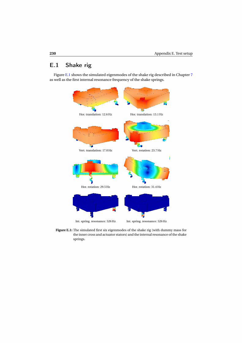
230 Appendix E. Test setup

E.1 Shake rig

Figure E.1 shows the simulated eigenmodes of the shake rig described in Chapter 7as well as the first internal resonance frequency of the shake springs.

Hor. translation: 12.6 Hz Hor. translation: 13.1 Hz

Vert. translation: 17.0 Hz Vert. rotation: 23.7 Hz

Hor. rotation: 29.5 Hz Hor. rotation: 31.4 Hz

Int. spring. resonance: 526 Hz Int. spring. resonance: 526 Hz

Figure E.1: The simulated first six eigenmodes of the shake rig (with dummy mass forthe inner cross and actuator stators) and the internal resonance of the shakesprings.

E.2: Active wrench 231

E.2 Active wrench

The active wrench as measured in Section 7.7 result from the actuator forcesaccording (E.1). The directly measured active wrench is shown in Fig. E.2.

(a) (d)

(b) (e)

(c) (f)

Figure E.2: The measured active wrench ~wact. The measured planes are at z =−0.5mm(yellow), z = 0.0mm (orange) and z = 0.5mm (red).


E.3 Transformation matrices

The transformation matrix that has been used to transform the individual actuatorforces F1h . . .F3v to a wrench on the isolated platform’s CoG is defined by

Fx

Fy

Fz

Tx

Ty

Tz

=

cos(π3 ) cos(π3 ) −1sin(π3 ) −sin(π3 ) 0

0 0 0−sin(π3 )(hh −hg c ) sin(π3 )(hh −hg c )cos(π3 )(hh −hg c ) cos(π3 )(hh −hg c ) (hh −hg c )

rh rh rh

. . .

. . .

0 0 00 0 01 1 1

−sin(π6 )rv −sin(π6 )rv rv

−cos(π6 )rv cos(π6 )rv 00 0 0

F1h

F2h

F3h

F1v

F2v

F3v

. (E.1)

The variables are defined in Section 7.5.4.

E.4 Material properties

Table E.1 summarizes some important typical and minimum remanence andcoercivity values of transverse-field pressed material. The typical remanent fluxdensity and typical coercivity have been used to obtain the relative permeabilityµrtyp of the last column, which is approximately 1.03 for all materials. The materialproperties of Vacodym 854 TP are shown in Table E.3 and Fig. E.3.

E.4: Material properties 233

Table E.1: Characteristic properties of transverse-field pressed hard magnetic materi-als [180] and the typical relative permeability obtained from these data.

Brtyp Brmin Hcbtyp Hcbmin µrtyp

745 TP 1.41 1.37 1090 1035 1.0294764 TP 1.37 1.33 1060 1005 1.0285776 TP 1.32 1.28 1020 970 1.0298837 TP 1.37 1.33 1060 1010 1.0285854 TP 1.32 1.28 1020 970 1.0298863 TP 1.29 1.25 995 950 1.0317872 TP 1.25 1.21 965 915 1.0308890 TP 1.19 1.15 915 865 1.0349633 TP 1.32 1.28 1020 970 1.0298655 TP 1.26 1.22 970 925 1.0337669 TP 1.22 1.17 940 875 1.0328677 TP 1.18 1.13 915 860 1.0262688 TP 1.14 1.09 885 830 1.0251

Table E.2: Physical properties of aluminum and stainless steel.

Description Aluminum Stainless steelMass density 2.7 ·103 kg/m3 8.0 ·103 kg/m3

Thermal conductivity 235 W/(mK) 14.6 W/(mK)Resistivity (20) 2.8 ·10−8Ωm 74 ·10−8Ωm

Table E.3: Characteristic properties of Vacodym 854TP [180].

Property Symbol [unit] Min. Typ. Max.Remanence Br [T] 1.28 1.32Coercivity Hcb [kA/m] 970 1020Intrinsic coercivity Hci [kA/m] 1670Remanence temperature coefficient Br [%/C] -0.105Coercivity temperature coefficient Hci [%/C] -0.60Mass density ρ [g/cm3] 7.7Electrical resistivity ρ [Ωm] 1.2 1.6


VACODYM 854 TP

-0,5

20° C

120 ° C 150 ° C 180 ° C80° C60° C 100 ° C

-0,8

-0,6

-0,4

-0,2

0,0

0,2

0,4

0,6

0,8

1,0

1,2

1,4

1,6

-2 0 - 18 -16 -14 -12 -10 -8 -6 -4 -2 0

-8

-6

-4

-2

4

10

12

14

16

T kG

J,B

kOe

B/ µo H ·

kA/m -1400 -1200 -1000

0,4-0,2-5,1-0,1-

H

0-800 -600 -400 -200

8

6

2

0

Figure E.3: Typical demagnetization curves for Vacodym 854TP [180].

E.5: Equipment properties 235

E.5 Equipment properties

Table E.4: Equipment used in the measurements.

Description Manufacturer TypeData acquisition system Speedgoat xPC Target systemAmplifiers of the shake actuators Prodrive QUAD 260/50Amplifiers of the vibration isolator Prodrive 3AX 52/6Optical position sensors Philtec RC100-AELNAccelerometers Kistler 8330M04Shake actuators BEI Kimco LA50-65-01ZPT100 temp. readout Agilent 34970A

Table E.5: Physical properties of the data acquisition system.

Description Type ValueCore Core2Duo 3.33GHz / 2048MB RAMAnalog inputs IO106 64-channel 16-bit parallel conversionSerial communication IO504 8-channel RS485

Table E.6: Physical properties of the power amplifiers.

Description 3AX QUADConverter type PWM PWMBandwidth 4 kHz 6 kHzCurrent (rms) 2 A ACurrent (max) ±6A ±12.5AVoltage (max) ±52V ±260VInterface RS485 (5.5 Mbps) RS485 (5.5 Mbps)DC-link GEN60-40-1P230 GEN500-30-MD-3P400

(60 V - 40 A) (500 V - 30 A)

Table E.7: Physical properties of the optical position sensors.

Description ValueType Philtec RC100-AELNRange 0-5 mmSpot size Ø 2.5 mmResolution 0.75µmNominal sensitivity 1.3mV/µm


Table E.8: Physical properties of the accelerometers.

Description ValueType Kistler 8330M04Range ±3gResolution < 1.3µgNominal sensitivity 1200mV/gLinearity ±0.1%Frequency response ±5% 0. . .1000HzFrequency response ±3dB 0. . .2500Hz

Table E.9: Physical properties of the shake actuators.

Description ValueType BEI Kimco LA50-65-001ZForce constant 124.1 N/ABack EMF constant 125 V/(m/s)DC Resistance 4.6ΩAC inductance (1 kHz) 5.3 mHActuator constant 57N/

pW

Coil assembly weight 1.45 kgField assembly weight 11 kg

Table E.10: Physical properties of the amplifiers used for the accelerometer signals.

Description ValueType Krohn-Hite Model 3364Mode Low-pass 4-poleAttenuation 24 dB/decPre-filter gain 0 dB-50 dBPost-filter gain 0 dB-20 dB

Table E.11: Physical properties of the readout device of the PT100 sensors.

Description ValueType Agilent 34970AMeasurement 4-wire PT100Multiplexer Agilent 34901A, 20 channels

237

Nomenclature

Symbols

Symbol [Unit] Quantity Page~A [Vs/m] Magnetic vector potential . . . . . . . . . . . . . . . . . . . . . . . . . .26~B [T] Magnetic flux density . . . . . . . . . . . . . . . . . . . . . . . . . . . . . . 24~Br [T] Remanent magnetic flux density . . . . . . . . . . . . . . . . . . 25b [Ns/m] Damping constant . . . . . . . . . . . . . . . . . . . . . . . . . . . . . . . . . 89~c [−] Nonlinear inequality constraint vector . . . . . . . . . . . 110~ceq [−] Nonlinear equality constraint vector . . . . . . . . . . . . . 110~D [C/m2] Electrical flux density . . . . . . . . . . . . . . . . . . . . . . . . . . . . . . 24di [m] Inner cross support thickness . . . . . . . . . . . . . . . . . . . . 131do [m] Outer cross support thickness . . . . . . . . . . . . . . . . . . . . 131dwi [m] Copper diameter of wire . . . . . . . . . . . . . . . . . . . . . . . . . . 159dwo [m] Outer diameter of wire . . . . . . . . . . . . . . . . . . . . . . . . . . . .158~E [V/m] Electrical field strength . . . . . . . . . . . . . . . . . . . . . . . . . . . . 24~F [N] Force . . . . . . . . . . . . . . . . . . . . . . . . . . . . . . . . . . . . . . . . . . . . . . . 33~f [N/m3] Force density . . . . . . . . . . . . . . . . . . . . . . . . . . . . . . . . . . . . . . . 33~fs [N/m2] Surface force density . . . . . . . . . . . . . . . . . . . . . . . . . . . . . . . 59f [Hz] Frequency . . . . . . . . . . . . . . . . . . . . . . . . . . . . . . . . . . . . . . . . 162fr [Hz] Resonance frequency . . . . . . . . . . . . . . . . . . . . . . . . . . . . . 104g [m/s2] Acceleration due to gravity . . . . . . . . . . . . . . . . . . . . . . . 104Ht (s) [−] Transmissibility transfer function . . . . . . . . . . . . . . . . 213Hc (s) [1/kg] Compliance transfer function . . . . . . . . . . . . . . . . . . . . 215~H [A/m] Magnetic field strength . . . . . . . . . . . . . . . . . . . . . . . . . . . . 24~Hcb [A/m] Coercivity . . . . . . . . . . . . . . . . . . . . . . . . . . . . . . . . . . . . . . . . . . 31~Hci [A/m] Intrinsic coercivity . . . . . . . . . . . . . . . . . . . . . . . . . . . . . . . . . 31h [m] Height . . . . . . . . . . . . . . . . . . . . . . . . . . . . . . . . . . . . . . . . . . . . .128hb [m] Coil bundle height . . . . . . . . . . . . . . . . . . . . . . . . . . . . . . . . 156hg [m] Airgap height . . . . . . . . . . . . . . . . . . . . . . . . . . . . . . . . . . . . . 109hm [m] Magnet height . . . . . . . . . . . . . . . . . . . . . . . . . . . . . . . . . . . . 109i [A] Electrical current . . . . . . . . . . . . . . . . . . . . . . . . . . . . . . . . . 158~J [A/m2] Electrical volume current density . . . . . . . . . . . . . . . . . .24


Symbol [Unit] Quantity Page~Jm [A/m2] Equivalent magnetic volume current density . . . . . 26J [−] Jacobian . . . . . . . . . . . . . . . . . . . . . . . . . . . . . . . . . . . . . . . . . . . . 62~jm [A/m] Equivalent magnetic surface current density . . . . . . 40K [N/m] Stiffness matrix . . . . . . . . . . . . . . . . . . . . . . . . . . . . . . . . . . . . .62k [N/m] Stiffness . . . . . . . . . . . . . . . . . . . . . . . . . . . . . . . . . . . . . . . . . . . . 89k [N/A] Actuator force constant . . . . . . . . . . . . . . . . . . . . . . . . . . . 161L [H] Inductance . . . . . . . . . . . . . . . . . . . . . . . . . . . . . . . . . . . . . . . .158lb [m] Coil bundle width . . . . . . . . . . . . . . . . . . . . . . . . . . . . . . . . .156lci [m] Coil core length . . . . . . . . . . . . . . . . . . . . . . . . . . . . . . . . . . . 156lco [m] Outer coil length . . . . . . . . . . . . . . . . . . . . . . . . . . . . . . . . . . 156lh [m] Halbach magnet length . . . . . . . . . . . . . . . . . . . . . . . . . . . 156lm [m] Magnet length . . . . . . . . . . . . . . . . . . . . . . . . . . . . . . . . . . . . 156lw [m] Wire length . . . . . . . . . . . . . . . . . . . . . . . . . . . . . . . . . . . . . . . 159~M [A/m] Magnetization . . . . . . . . . . . . . . . . . . . . . . . . . . . . . . . . . . . . . 25M [−] Rotation matrix . . . . . . . . . . . . . . . . . . . . . . . . . . . . . . . . . . . . 70m [kg] Mass . . . . . . . . . . . . . . . . . . . . . . . . . . . . . . . . . . . . . . . . . . . . . . . .89~m [Am2] Magnetic dipole moment . . . . . . . . . . . . . . . . . . . . . . . . . . 29N [−] Number of turns . . . . . . . . . . . . . . . . . . . . . . . . . . . . . . . . . . 158n [−] Number of poles . . . . . . . . . . . . . . . . . . . . . . . . . . . . . . . . . . 111~P [C/m2] polarization . . . . . . . . . . . . . . . . . . . . . . . . . . . . . . . . . . . . . . . . 25P [W] Power . . . . . . . . . . . . . . . . . . . . . . . . . . . . . . . . . . . . . . . . . . . . . 158P (s) [−] Passive sensitivity function . . . . . . . . . . . . . . . . . . . . . . . 216Q(s) [−] Passive complementary sensitivity function . . . . . 216q [C] Electrical charge . . . . . . . . . . . . . . . . . . . . . . . . . . . . . . . . . . . 33~r [m] Arm . . . . . . . . . . . . . . . . . . . . . . . . . . . . . . . . . . . . . . . . . . . . . . . . 33r1 [m] Half the thickness of gravity compensator leg . . . . 131r2 [m] Half the thickness of the gravity compensator . . . 131rc [m] Inner radius of coil corner . . . . . . . . . . . . . . . . . . . . . . . . 156R [Ω] Electrical resistance . . . . . . . . . . . . . . . . . . . . . . . . . . . . . . 158S [N2/W] Actuator steepness . . . . . . . . . . . . . . . . . . . . . . . . . . . . . . . .161

S [m2] Surface . . . . . . . . . . . . . . . . . . . . . . . . . . . . . . . . . . . . . . . . . . . . . 33~T [Nm] Torque . . . . . . . . . . . . . . . . . . . . . . . . . . . . . . . . . . . . . . . . . . . . . .33~t [Nm/m3] Torque density . . . . . . . . . . . . . . . . . . . . . . . . . . . . . . . . . . . . . 33~ts [Nm/m2] Surface torque density . . . . . . . . . . . . . . . . . . . . . . . . . . . . . 66t [s] Time . . . . . . . . . . . . . . . . . . . . . . . . . . . . . . . . . . . . . . . . . . . . . . . .24T [K] Temperature . . . . . . . . . . . . . . . . . . . . . . . . . . . . . . . . . . . . . . 147V [V] Voltage . . . . . . . . . . . . . . . . . . . . . . . . . . . . . . . . . . . . . . . . . . . . 158

V [m3] Volume . . . . . . . . . . . . . . . . . . . . . . . . . . . . . . . . . . . . . . . . . . . . . 25~v [m/s] Velocity . . . . . . . . . . . . . . . . . . . . . . . . . . . . . . . . . . . . . . . . . . . . .33W [J] Energy . . . . . . . . . . . . . . . . . . . . . . . . . . . . . . . . . . . . . . . . . . . . . .28~w [N,Nm] Wrench . . . . . . . . . . . . . . . . . . . . . . . . . . . . . . . . . . . . . . . . . . . .180w [m] Width . . . . . . . . . . . . . . . . . . . . . . . . . . . . . . . . . . . . . . . . . . . . . 110wi [m] Inner magnet spacing . . . . . . . . . . . . . . . . . . . . . . . . . . . . 131wo [m] Outer magnet spacing . . . . . . . . . . . . . . . . . . . . . . . . . . . . 131wci [m] Coil core width . . . . . . . . . . . . . . . . . . . . . . . . . . . . . . . . . . . .156


Symbol [Unit] Quantity Pagewco [m] Outer coil width . . . . . . . . . . . . . . . . . . . . . . . . . . . . . . . . . . 156wm [m] Magnet width . . . . . . . . . . . . . . . . . . . . . . . . . . . . . . . . . . . . . 156z0 [m] Vertical offset . . . . . . . . . . . . . . . . . . . . . . . . . . . . . . . . . . . . . 127

ε0 [As/(Vm)] Permittivity of free space . . . . . . . . . . . . . . . . . . . . . . . . . . .25εhc [−] Hot-cold effect . . . . . . . . . . . . . . . . . . . . . . . . . . . . . . . . . . . . . 77ζ [−] Copper fill factor . . . . . . . . . . . . . . . . . . . . . . . . . . . . . . . . . . 158ζ [−] Damping ratio . . . . . . . . . . . . . . . . . . . . . . . . . . . . . . . . . . . . . 90µ [H/m] Permeability . . . . . . . . . . . . . . . . . . . . . . . . . . . . . . . . . . . . . . . 25µ0 [H/m] Permeability of free space . . . . . . . . . . . . . . . . . . . . . . . . . .25µr [−] Relative permeability . . . . . . . . . . . . . . . . . . . . . . . . . . . . . . 25~λ [m3] Intermediate torque computation variable . . . . . . . .66Ξ [m] Intermediate stiffness computation variable . . . . . . 62ξ [m2] Intermediate force computation variable . . . . . . . . . 58ρe [Ωm] Specific electrical resistivity . . . . . . . . . . . . . . . . . . . . . . 159ρc [C/m3] Free charge density . . . . . . . . . . . . . . . . . . . . . . . . . . . . . . . . 24ρm [A/m2] Magnetic volume charge density . . . . . . . . . . . . . . . . . . 27σe [S/m] Electrical conductivity . . . . . . . . . . . . . . . . . . . . . . . . . . . . . 25σm [A/m] Magnetic surface charge density . . . . . . . . . . . . . . . . . . .41τe [s] Electrical actuator time constant . . . . . . . . . . . . . . . . . 160τm [m] Magnet pitch . . . . . . . . . . . . . . . . . . . . . . . . . . . . . . . . . . . . . .109τp [m] Pole pitch . . . . . . . . . . . . . . . . . . . . . . . . . . . . . . . . . . . . . . . . . 109Ψ [Wb] Flux linkage . . . . . . . . . . . . . . . . . . . . . . . . . . . . . . . . . . . . . . . 158ϕ [Wb] Magnetic flux . . . . . . . . . . . . . . . . . . . . . . . . . . . . . . . . . . . . . . 31χm [−] Magnetic susceptibility . . . . . . . . . . . . . . . . . . . . . . . . . . . . 25Ψ [A] Magnetic scalar potential . . . . . . . . . . . . . . . . . . . . . . . . . . 27ωn [rad/s] Natural frequency . . . . . . . . . . . . . . . . . . . . . . . . . . . . . . . . . . 90

G [−] Objective function . . . . . . . . . . . . . . . . . . . . . . . . . . . . . . . . 110

T [N/m2] Maxwell stress tensor . . . . . . . . . . . . . . . . . . . . . . . . . . . . . . 34


Abbreviations

Abbreviation Explanation2D Two-dimensional3D Three-dimensionalANA AnalyticalAP Axial pressedBEM Bounday Element MethodCoA Center of ActuationCoG Center of GravityCoM Center of massDoF Degree of FreedomFDM Finite Difference MethodFEM Finite Element MethodFVM Finite Volume MethodMEA MeasuredMEC Magnetic Equivalent CircuitMST Maxwell stress tensorSQP Sequential Quadratic ProgrammingTP Transverse pressedVC Vibration Criterion

Subscripts

Subscript Explanationact Activeavg Average

diss Dissipatedext Externalem Electromagneticgrav Gravitationalhor Horizontalin Input

mech Mechanicalmag Magneticmax Maximum valuemin Minimum valueout Outputpos Positionpot Potentialprim Primarysec Secondarytyp Typicalver Vertical


Operators

Operator Explanation∇ Gradient· Dot product× Cross product∇· Divergence∇× Curl

General definitions

Symbol [Unit] Quantity Page~ex ,~ey ,~ez [−] Unit vectors along the cartesian axes . . . . . . . . . . . . . . 48~n [−] Outward pointing normal unit vector . . . . . . . . . . . . . 34~O [−] Origin . . . . . . . . . . . . . . . . . . . . . . . . . . . . . . . . . . . . . . . . . . . . . . 48

S [m2] Surface . . . . . . . . . . . . . . . . . . . . . . . . . . . . . . . . . . . . . . . . . . . . . 33V [m3] Volume . . . . . . . . . . . . . . . . . . . . . . . . . . . . . . . . . . . . . . . . . . . . . 25

243

Index

AActive isolation . . . . . . . . . . . . . . . . . 92, 216Actuator

Coil current definition. . . . . . . . .156Cooling facilities. . . . . . . . . . . . . . .173External units. . . . . . . . . . . . . . . . . .174Integration . . . . . . . . . . . . . . . 166, 172Placement . . . . . . . . . . . . . . . . 154, 170

Amperian model . . . . . . . . . . . . . . . . . . . . . 40Analytical

Field calculation . . . . . . . . . . . . 47, 51Force calculation . . . . . . . . . . . . . . . 49Stiffness calculation . . . . . . . . . . . . 62Torque calculation. . . . . . . . . . . . . .65

BBiot-Savart law . . . . . . . . . . . . . . . . . . . . . 159Boundary conditions . . . . . . . . . . . . 28, 43Boundary Element Method . . . . . . . . . . 38

CCenter of

Actuation . . . . . . . . . . . . . . . . . 156, 179Gravity . . . . . . . . . . . . . . . . . . . . 171, 179

ChargeMagnetic . . . . . . . . . . . . . . . . . . . . . . . .30Surface density. . . . . . . . . . . . . .41, 55

Checkerboard array . . . . . . . . . . . . . . . . 111Chipping . . . . . . . . . . . . . . . . . . . . . . . . . . . . . 76Coercivity . . . . . . . . . . . . . . . . . . . . . . . 31, 145

intrinsic . . . . . . . . . . . . . . . . . . . . . . . . . 31Coil

Electrical time constant . . . . . . . 160Fill factor . . . . . . . . . . . . . . . . . . . . . . 158Inductance . . . . . . . . . . . . . . . . . . . . 159Orthocyclic winding. . . . . . . . . . .158

Resistance . . . . . . . . . . . . . . . . . . . . . 159Compliance . . . . . . . . . . . . . . . . . . . . . 91, 215Conformal mapping . . . . . . . . . . . . . . . . . 42Constitutive relations . . . . . . . . . . . . 24, 25Coordinate rotation. . . . . . . . . . . . . . . . . .70Coulomb gauge . . . . . . . . . . . . . . . . . . . . . . 26Coulombian model . . . . . . . . . . . . . . . . . . 40Cross

Inner – . . . . . . . . . . . . . . . . . . . . . . . . . 131Outer –. . . . . . . . . . . . . . . . . . . . . . . . .131

Cross-shaped topology . . . . . . . . . . . . . 131Cuboidal magnets . . . . . . . . . . . . . . . . . . . 47Current sheet model . . . . . . . . . . . . . . . . . 40

DDamping

Critical . . . . . . . . . . . . . . . . . . . . . . . . . . 90Eddy currents . . . . . . . . . . . . . . . . . . . 94Low electromagnetic – . . . . . . . . . 97

Demagnetization . . . . . . . . . . . . . . . 77, 225Demagnetizing field . . . . . . . . . . . . . . . . . 31Diamagnetics . . . . . . . . . . . . . . . . . . . . . . . 222Dipole . . . . . . . . . . . . . . . . . . . . . . . 25, 29, 220Discretization

Surface . . . . . . . . . . . . . . . . . . . . . . . . . . 38Undiscretized . . . . . . . . . . . . . . . . . . . 39Volume . . . . . . . . . . . . . . . . . . . . . . . . . 35

Dynamic levitation . . . . . . . . . . . . . . . . . 223

EEarnshaw’s theorem . . . . . . . . . . . . 95, 220

Ways around Earnshaw . . . . . . . 221Energy . . . . . . . . . . . . . . . . . . . . . . . . . . . . 28, 34

Electromagnetic . . . . . . . . . . . . . . . . 28Magnetostatic . . . . . . . . . . . . . . . . . . 32Product . . . . . . . . . . . . . . . . . . . . . . . . . 32

244 Index

FFeedback control . . . . . . . . . . . . . . . 92, 216

stabilization . . . . . . . . . . . . . . . . . . . 224Field calculation

Arc-shaped magnets . . . . . . . . . . . .50Axial magnetization . . . . . . . . . . . . 50Cuboidal magnets . . . . . . . . . . . . . . 47Pyramidal frustum. . . . . . . . . . . . . .54Radial magnetization . . . . . . . . . . . 51Rectangular sheet. . . . . . . . . . . . . . .47Ring-shaped magnets . . . . . . . . . . 50Triangular surface . . . . . . . . . . . . . . 51

Figure of merit . . . . . . . . . . . . . . . . . . . . . . . 32Finite

Differences Method . . . . . . . . . . . . 36Element Method . . . . . . . . . . . . . . . . 35Volume Method . . . . . . . . . . . . . . . . 36

Flux density . . . . . . . . . . . . . . . . . . . . . . . . . . 24Remanent . . . . . . . . . . . . . . . 25, 74, 77

Flux tube . . . . . . . . . . . . . . . . . . . . . . . . . . . . . 37Force

Analytical . . . . . . . . . . . . . . . . . . . 49, 57Lorentz . . . . . . . . . . . . . . . . . . . . . . . . . 33Maxwell stress tensor . . . . . . . . . . . 34Parallel magnetization. . . . . . . . . .57Perpendicular magnetization . . 59Rotated magnets. . . . . . . . . . . . . . . .49Virtual work . . . . . . . . . . . . . . . . . . . . 34

Fourier model. . . . . . . . . . . . . . . . . . . . . . . .39

GGravity compensator . . . 17, 97, 104, 171

Cross shape. . . . . . . . . . . . . . . . . . . .131Inner cross. . . . . . . . . . . . . . . .131, 172Legs. . . . . . . . . . . . . . . . . . . . . . . . . . . .130Outer cross . . . . . . . . . . . . . . . 131, 172

Green’s Function . . . . . . . . . . . . . . . . . . . . . 26Green’s function . . . . . . . . . . . . . . . . . . 26, 27

HHalbach. . . . . . . . . . . . .see Quasi-HalbachHarmonic model. . . . . . . . . . . . . . . . . . . . .39Hot-cold effect . . . . . . . . . . . . . . . . . . 76, 146Hysteresis loop. . . . . . . . . . . . . . . . . . . . . . .31Hysterigraph . . . . . . . . . . . see HystographHystograph . . . . . . . . . . . . . . . . . . . . . . . . . . 74

IInner cross . . . . . . . . . . . . . . . . . . . . . 131, 171

JJacobian. . . . . . . . . . . . . . . . . . . . . . . . . . . . . .62

LLaplace’s Equation . . . . . . . . . . . . . . . . . . . 26LCR circuits . . . . . . . . . . . . . . . . . . . . . . . . . 223Leg . . . . . . . . . . . . . . . . . . . . . . . . . . . . . . . . . . 130Levitation . . . . . . . . . . . . . . . . . . . . . . . 95, 219Load line . . . . . . . . . . . . . . . . . . . . . . . . 77, 147Lorentz force . . . . . . . . . . . . . . . . . . . . . . . . . 33

MMachine voltage equation . . . . . . . . . . 158Magnet

Ageing . . . . . . . . . . . . . . . . . . . . . . . . . . 77Chipping. . . . . . . . . . . . . . . . . . . . . . . .76Stacking . . . . . . . . . . . . . . . . . . . . . . . 126

Magnet arrayCheckerboard . . . . . . . . . . . . . . . . . 111Quasi-Halbach . . . . . . . . . . . . . . . . 115Unequal dimensions . . . . . . . . . . 117

MagneticDomains . . . . . . . . . . . . . . . . . . . . . . . . 29Energy. . . . . . . . . . . . . . . . . . . . . . .32, 34Equivalent Circuit . . . . . . . . . . . . . . 37Imaging . . . . . . . . . . . . . . . . . . . . . . . . . 43Levitation . . . . . . . . . . . . . . . . . . . . . . . 95Nodes . . . . . . . . . . . . . . . . . . . . . . . 60, 96Suspension . . . . . . . . . . . . . . . . . . . . . 95

Magnetization . . . . . . . . . . . . . . . . . . . . . . . 25Misalignment . . . . . . . . . . 75, 76, 145

Magnetostatics . . . . . . . . . . . . . . . . . . . . . . 25Maxwell stress tensor . . . . . . . . . . . . . . . . 34Maxwell’s equations . . . . . . . . . . . . . . . . . 24Meissner-Ochsenfeld effect . . . . . . . . 222Meshing. . . . . . . . . . . . . . . . . . . . . . . . . . . . . .35Metrology . . . . . . . . . . . . . . . . . . . . . . . . . . . . 16Misalignment . . . . . . . . . . . . . . 75, 145, 146Modeling inaccuracies . . . . . . . . . . 74, 144Modularity . . . . . . . . . . . . . . . . . . . . . 126, 148Motor force constant . . . . . . . . . . . . . . . 161

OOptimization . . . . . . . . . . . . . . . . . . . . . . . 110

Index 245

Front. . . . . . . . . . . . . . . . . . . . . . . . . . .111Oscillating fields . . . . . . . . . . . . . . . . . . . . 223Outer cross . . . . . . . . . . . . . . . . . . . . 131, 171

PParallel magnetization . . . . . . . . . . . . . . . 57Passive vibration isolation . . . . . . 89, 213Permeability

Free space . . . . . . . . . . . . . . . . . . . . . . 25Relative. . . . . . . . . . . . . . . . .25, 75, 144

Perpendicular magnetization. . . . . . . .57Poisson’s Equation . . . . . . . . . . . . . . . . . . . 26Potential

Magnetic scalar – . . . . . . . . . . . . . . . 27Magnetic vector – . . . . . . . . . . . . . . . 26

Pre-compression . . . . . . . . . . . . . . . . . . . 214Pyramidal Frustum . . . . . . . . . . . . . . . . . . 54

QQuasi-Halbach . . . . . . . . . . . . . . . . 115, 156Quasi-Static Field Theory. . . . . . . . . . . .26

RRemanent flux density. . . . . . . . . . . . . .144Rotation matrix . . . . . . . . . . . . . . . . . . 55, 70

SSensitivity function . . . . . . . . . . . . 216, 218

Complementary – . . . . . . . . . . . . . 216Sensors

Acceleration . . . . . . . . . . . . . . . . . . . 178Position. . . . . . . . . . . . . . . . . . . . . . . .178

Sommerfeld convention . . . . . . . . . . . . . 25Spin-stabilized magnetic levitation 223Stability . . . . . . . . . . . . . . . . . . . . . . . . . . . . . . 95

Criteria . . . . . . . . . . . . . . . . . . . . . . . . 219Methods . . . . . . . . . . . . . . . . . . . . . . . 222

Static analysis . . . . . . . . . . . . . . . . . . . . . . . . 26Static Field Theory . . . . . . . . . . . . . . . . . . . 26Stator . . . . . . . . . . . . . . . . . . . . . . . . . . . . . . . 172Steepness . . . . . . . . . . . . . . . . . . . . . . . . . . . 161Stiffness

Low-dynamic . . . . . . . . . . . . . . . . . . . 93Matrix . . . . . . . . . . . . . . . . . . . . . . . . . . .62Negative . . . . . . . . . . . . . . . . . . . . . . . . 93Parallel magnetization. . . . . . . . . .63Perpendicular magnetization . . 64

Quasi-zero . . . . . . . . . . . . . . . . . . . . . . 93Stray field . . . . . . . . . . . . . . . . . . . . . . . . . . . . 31Subdomain model . . . . . . . . . . . . . . . . . . . 39Superconduction . . . . . . . . . . . . . . . . . . . 222Superposition. . . . . . . . . . . . .42, 49, 55, 72Surface charge model . . . . . . . . . . . . . . . . 41Suspension . . . . . . . . . . . . . . . . . . . . . . . . . . 95

TTemperature effects . . . . . . . .78, 147, 182Tolerances . . . . . . . . . . . . . . . . . . . 74, 76, 144

Global . . . . . . . . . . . . . . . . . . . . . . . . . . .74Local . . . . . . . . . . . . . . . . . . . . . . . . . . . . 75

Torque . . . . . . . . . . . . . . . . . . . . . . . . . . . . . . . 65Lorentz . . . . . . . . . . . . . . . . . . . . . . . . . 33Parallel magnetization. . . . . . . . . .67Perpendicular magnetization . . 68

Translator . . . . . . . . . . . . . . . . . . . . . . . . . . .172Transmissibility . . . . . . . . . . . . . . . . . 90, 213Tuned LCR circuits . . . . . . . . . . . . . . . . . 223

VVacodym. . . . . . . . . . . . . . . . . . . . . . . . . . . .134Vertical airgaps . . . . . . . . . . . . . . . . . 99, 125Vibration criteria . . . . . . . . . . . . . . . . . . . . 88Vibration isolation system . . . . . . . . . . . 95Vibration isolator . . . . . . . . . . . . . . . 95, 171Vibration sources . . . . . . . . . . . . . . . . . . . . 87Virgin curve . . . . . . . . . . . . . . . . . . . . . . . . . . 31Virtual work. . . . . . . . . . . . . . . . . . . . . . . . . .34Voltage equation. . . . . . . . . . . . . . . . . . . .158

WWinding

Inductance . . . . . . . . . . . . . . . . . . . . 159Orthocyclic . . . . . . . . . . . . . . . . . . . . 158Resistance . . . . . . . . . . . . . . . . . . . . . 159

WorkingEnvelope. . . . . . . .105, 128, 135, 183Point . . . . . . . . . . . . . . . . . . 77, 128, 135

Working envelope . . . . . . . . . . . . . . . . . . 101Wrench. . . . . . . . . . . . . . . . . . . . . . . . . .72, 180

Active . . . . . . . . . . . . . . . . . . . . . . . . . . 183

246 Index

247

References

[1] Feng shui corner. http:// www.fengshuicorner.com. Cited on page 12.

[2] J. S. Agashe and D. P. Arnold. A study of scaling and geometry effects onthe forces between cuboidal and cylindrical magnets using analytical forcesolutions. J. Phys. D: Appl. Phys., 41(105001):1–9, 2008. Cited on pages 49and 99.

[3] G. Akoun and J.-P. Yonnet. 3D analytical calculation of the forces exertedbetween two cuboidal magnets. IEEE Trans. on Magn., 20(5):1962–1964,September 1984. Cited on pages 15, 43, 48, 49, 50, 57, 58, 62, 73, and 96.

[4] P. Alabuzhev, A. Gritchin, L. Kim, G. Migirenko, V. Chon, and P. Stephanov.Vibration Protecting and Measuring Systems with Quasi-Zero Stiffness. Hemi-sphere, New York, 1st edition, 1989. ISBN 0-89116-811-7. Ed. by E. Rivin. Citedon page 93.

[5] H. Allag and J.-P. Yonnet. 3D analytical calculation of interactions betweenperpendicularly magnetized magnets: Application to any magnetizationdirection. Sensor letters, 7(4):486–491, August 2009. Cited on pages 49, 59,and 73.

[6] H. Allag and J.-P. Yonnet. 3-D analytical calculation of the torque and forceexerted between two cuboidal magnets. IEEE Trans. on Magn., 45(10):3969 –3972, October 2009. Cited on pages 49 and 66.

[7] H. Allag, J.-P. Yonnet, and M. E. H. Latreche. Analytical calculation of the torqueexerted between two perpendicularly magnetized magnets. J. of Appl. Phys.,109:07E701, March 2011. Cited on pages 66 and 68.

[8] H. Amick, M. Gendreau, T. Busch, and C. G. Gordon. Evolving criteria forresearch facilities: I - vibration. In Proceedings of the SPIE Conf., volume 5933,pages 302–305, San Diego, California, July 2005. Cited on pages 16, 87, and 88.

[9] C. G. Anderson and S. H. Salter. Optimum geometry analyses for rectangularhard magnet pairs. IEEE Trans. on Magn., 23(5):3836–3844, September 1987.Cited on page 99.

248 References

[10] R. Appunn, B. Schmulling, and K. Hameyer. Electromagnetic guiding of verticaltransportation vehicles: Experimental evaluation. IEEE Trans. on IndustrialElectronics,, 57(1):335 –343, January 2010. Cited on page 98.

[11] V. Arkadiev. A floating magnet. Nature, 160(4062):330, September 1947. Citedon page 223.

[12] F. Auer. Combined electromagnetic suspension and propulsion for positioningwith sub-micrometer accuracy. PhD thesis, Delft University of Technology, 1995.Cited on pages 95, 98, and 222.

[13] B. de Kraker and D. H. van Campen. Mechanical Vibrations. Shaker Publishing,Maastricht, The Netherlands, 1st edition, 2001. Cited on pages 15, 193, and 205.

[14] S. Babic and M. M. Gavrilovic. New expression for calculating magnetic fieldsdue to current-carrying solid conductors. IEEE Trans. on Magn., 33(5):4134–4136, September 1997. Cited on pages 50 and 51.

[15] S. I. Babic and C. Akyel. Improvement in the analytical calculation of themagnetic field produced by permanent magnet rings. Prog. in ElectromagneticsRes. C, 5:71–82, 2008. Cited on pages 50 and 51.

[16] S. I. Babic and C. Akyel. Magnetic force calculation between thin coaxial circularcoils in air. IEEE Trans. on Magn., 44(4):445 –452, April 2008. Cited on page 51.

[17] F. Bancel. Magnetic nodes. J. of Appl. Phys., 32:2155–2161, June 1999. Cited onpages 50, 51, 61, and 96.

[18] W. Baran. Analytical methods for the design calculation of p.m. synchronouscouplings. Acta Polytechnics Scandinavica, Applied Physics, 138:13–19, 1983.Cited on page 49.

[19] M. V. Berry. The levitron: an adiabatic trap for spins. Proc. R. Soc. London, Ser.A, 452(1948):1207–1220, May 1996. Cited on pages 222 and 223.

[20] M. V. Berry and A. K. Geim. Of flying frogs and levitrons. Eur. J. Phys., 18(4):307–313, May 1997. Cited on pages 219, 221, and 222.

[21] K. J. Binns, P. J. Lawrenson, and C. W. Trowbridge. The analytical and numericalsolution of electric and magnetic fields. Wiley, Chichester, 1st edition, 1992.Cited on pages 35 and 42.

[22] G. H. Blackwood. Active vibration isolation for controlled flexible structures. PhDthesis, Massachusetts Institute of Technology, 1993. Cited on pages 92, 216,and 217.

[23] H. Bleuler. A survey of magnetic levitation and magnetic bearing types. JSMEInt. J. Ser. III, 35(3):335–342, 1992. Cited on pages 94, 95, and 97.

[24] A. H. Boerdijk. Technical aspects of levitation. Philips Research Reports, 11:45–56, 1956. Cited on pages 95 and 222.

References 249

[25] E. Bonisoli and A. Vigliani. Passive elasto-magnetic suspensions: nonlinearmodels and experimental outcomes. Mechanics Research Communications, 34:385–394, 2007. Cited on page 92.

[26] F. J. Börgermann, R. Blank, G. W. Reppel, J. Bahrdt, and J. Pflüger. Improvedhomogeneity of permanent magnets for undulators and wigglers. In EuropeanParticle Accelerator Conference, pages 2234–2236, Genoa, Italy, June 2008. Citedon page 76.

[27] W. Braunbek. Freischwebende körper im elektrischen und magnetischen feld.Zeitschrift für Physik, 112(4):753–763, April 1939. Cited on pages 95, 219, 220,221, 222, and 223.

[28] W. Braunbek. Freies schweben diamagnetischer körper im magnetfeld.Zeitschrift für Physik, 112(4):764–769, April 1939. Cited on pages 95 and 222.

[29] H. Butler, F. Auer, M. van Duijnhoven, P. J. H. Meijers, J. G. C. van der Toorn, andJ. de Pee. Support device and lithographic apparatus. Patent no. 2006/0126040A1, June 2006. Cited on pages 17 and 94.

[30] S. D. Calverley. Design of a high speed switched reluctance machine forautomotive turbo-generator applications. PhD thesis, University of Sheffield,2001. Cited on page 36.

[31] A. Carrella, M. J. Brennan, and T. P. Waters. Static analysis of a passive vibrationisolator with quasi-zero-stiffness characteristic. Journal of Sound and Vibration,301(3-5):678 – 689, 2007. Cited on page 93.

[32] A. Carrella, M. J. Brennan, T. P Waters, and K. Shin. On the design of ahigh-static-low-dynamic stiffness isolator using linear mechanical springs andmagnets. Journal of Sound and Vibration, 315(3):712 – 720, 2008. Cited on page97.

[33] Flux 10 User’s guide. Cedrat Corporation, Grenoble, 2010. Release 10.3.3. Citedon pages 143 and 211.

[34] M. V. K. Chari and S. J. Salon. Numerical methods in electromagnetism.Academic Press, San Diego, 2000. Cited on pages 35 and 40.

[35] J. F. Charpentier and G. Lemarquand. Calculation of ironless permanent magnetcouplings using semi-numerical magnetic pole theory method. COMPEL, 20(1):72–89, January 2001. Cited on pages 50, 73, and 81.

[36] K. B. Choi, Y. G. Cho, T. Shinshi, and A. Shimokohbe. Stabilization of one degree-of-freedom control type levitation table with permanent magnet repulsiveforces. Mechatronics, 13:587–603, 2003. Cited on pages 98, 99, 117, and 118.

[37] Y.-M. Choi, M. G. Lee, D.-G. Gweon, and J. Jeong. A new magnetic bearingusing halbach magnet arrays for a magnetic levitation stage. Review of ScientificInstruments, 80(045106):1–9, 2009. Cited on pages 98, 99, and 126.

250 References

[38] J. M. D. Coey. Rare-earth iron permanent magnets. Oxford Univ. Press, Oxford,UK, 1st edition, 1996. Cited on pages 13, 29, 35, 37, 40, and 49.

[39] Private communication. Cited on pages 134, 145, and 146.

[40] J. C. Compter. The design and application of industrial linear motors. EindhovenUniv. of Technology, Eindhoven, 2008. Cited on page 158.

[41] J. C. Compter, E. A. Lomonova, and J. Makarovic. Direct 3-D method forperformance prediction of a linear moving coil actuator with various topologies.Science, Measurement and Technology, IEE Proceedings, 150(4):183–191, July2003. Cited on pages 156 and 157.

[42] J. C. Compter, J. L. G. Janssen, and E.A. Lomonova. Ampere’s circuital 3-D modelfor non-cuboidal magnets. IEEE Trans. on Magn., 46(12):4009–4015, December2010. Cited on pages 49 and 51.

[43] R. Cooper, V. Neil, and W. Woodruff. Optimum permanent-magnet dimensionsfor repulsion applications. IEEE Trans. on Magn., 9(2):125 – 127, June 1973.Cited on pages 50, 99, and 109.

[44] I. Da Silva and O. Horikawa. Experimental development of a one-degree-of-freedom controlled magnetic linear bearing. IEEE Trans. on Magn., 41(1):4257–4260, November 2005. Cited on page 125.

[45] I. Da Silva and O. Horikawa. Stiffness improvement of a 1-D.O.F. controlledmagnetic linear bearing. ABCM Symposium Series in Mechatronics, 2:89–96,2006. Cited on page 98.

[46] A. D’Angola, G. Carbone, L. Mangialardi, and C. Serio. Non-linear oscillations ina passive magnetic suspension. International Journal of Non-Linear Mechanics,41(9):1039 – 1049, 2006. Cited on page 92.

[47] J. de Boeij. Multi-Level Contactless Motion System. PhD thesis, EindhovenUniversity of Technology, 2009. Cited on pages 13 and 14.

[48] C. A. L. de Hoon. Lithographic apparatus comprising a vibration isolationsupport device. US Patent no. 2008/0230677 A1, September 2008. Cited onpages 17 and 94.

[49] D. B. DeBra. Vibration isolation of precision machine tools and instruments.Annals of the CIRP, 41(2):711–718, 1992. Cited on pages 15, 17, 87, 91, 94,and 216.

[50] J. Delamare, J.-P. Yonnet, and E. Rulliere. A compact magnetic suspension withonly one axis control. IEEE Trans. on Magn., 30(6):4746 –4748, November 1994.Cited on page 98.

[51] N. Delson and J. Houston. Actuator with repulsive magnetic forces. US Patentno. 6,307,285 B1, October 2001. Cited on pages 99 and 117.

References 251

[52] J. van Dijk. Mechatronic design of hard-mount concepts for precisionequipment. In H. Ulbrich and L. Ginzinger, editors, Motion and VibrationControl, pages 315–324. Springer Netherlands, 2009. Cited on page 100.

[53] C. Ding. Vibration Isolation Control of a Contactless Electromagnetic SuspensionSystem. PhD thesis, Eindhoven University of Technology. To be published. Citedon page 180.

[54] C. Ding, J. L. G. Janssen, A. A. H. Damen, and P. P. J. van den Bosch. Modeling andcontrol of a 6-dof contactless electromagnetic suspension system with passivegravity compensation. In Proc. of the XIX International Conference on ElectricalMachines, pages 1–6, September 2010. Cited on page 180.

[55] I. Dolezel, P. Karban, and P. Solin. Integral Methods in low-frequencyelectromagnetics. Wiley, New York, 2009. Cited on page 35.

[56] T. A. Driscoll and L. N. Trefethen. Schwarz-Christoffel Mapping. CambridgeUniv. Press, Cambridge, UK, 2002. Cited on page 42.

[57] E. Durand. Magnétostatique. Masson, Paris, France, 1968. Cited on page 50.

[58] S. Earnshaw. On the nature of the molecular forces which regulate theconstitution of the luminuferous ether. Trans. Camb. Phil. Soc., VII:1:97–112,1839. Cited on pages 62, 95, 154, 220, and 221.

[59] D. Eckert, K. H. Muller, and M. Wolf. Ageing effects in sintered(Nd,Dy)15(Fe,Co,Mo,Al)77b8permanent magnets. Trans. Camb. Phil. Soc., VII:1:97–112, 1839. Cited on page 77.

[60] P. Elies and G. Lemarquand. Analytical optimization of the torque of apermanent-magnet coaxial synchronous coupling. IEEE Trans. on Magn., 34(4):2267–2273, July 1998. Cited on pages 13, 50, 73, and 81.

[61] P. Elies and G. Lemarquand. Comparison of the torque of flat airgapsynchronous couplings versus the magnetization direction of the magnets. IEEETrans. on Magn., 35(1):548–556, January 1999. Cited on pages 50, 73, and 81.

[62] L. Encica. Space-mapping optimization applied to the design of a novelelectromagnetic actuator for active suspension. PhD thesis, EindhovenUniversity of Technology, 2008. Cited on page 98.

[63] A. M. Forrest. Meissner and Ochsenfeld revisited. Eur. J. Phys., 4:117–118, 1983.Cited on pages 222 and 223.

[64] E. P. Furlani. Formulas for the force and torque of axial couplings. IEEE Trans.on Magn., 29(5):2295–2301, September 1993. Cited on pages 33 and 51.

[65] E. P. Furlani. Analysis and optimization of synchronous magnetic couplings. J.of Appl. Phys., 79(8):4692–4694, April 1996. Cited on page 51.

252 References

[66] E. P. Furlani. Permanent Magnet and Electromechanical Devices: materials,analysis and applications. Academic Press, London, 6th edition, 2001. Citedon pages 13, 14, 24, 26, 27, 28, 32, 33, 34, 35, 36, 40, 41, 48, 49, 50, 105, 159,and 226.

[67] E. P. Furlani, S. Reznik, and W. Janson. A three-dimensional field solution forbipolar cylinders. IEEE Trans. on Magn., 30(5):2916–2919, September 1994.Cited on page 51.

[68] E.P. Furlani. A formula for the levitation force between magnetic disks. IEEETrans. on Magn., 29(6):4165–4169, November 1993. Cited on page 51.

[69] E.P. Furlani. A two-dimensional analysis for the coupling of magnetic gears.IEEE Trans. on Magn., 33(3):2317 –2321, May 1997. Cited on page 51.

[70] E.P. Furlani, S. Reznik, and A. Kroll. A three-dimensional field solution forradially polarized cylinders. IEEE Trans. on Magn., 31(1):844 –851, January 1995.Cited on page 51.

[71] E.P. Furlani, R. Wang, and H. Kusnadi. A three-dimensional model forcomputing the torque of radial couplings. IEEE Trans. on Magn., 31(5):2522 –2526, September 1995. Cited on page 51.

[72] C. G. Gordon. Dynamics of advanced technology facilities: A historicalperspective. In Proc. of 12th ASCE Eng. Mechanics Conf., pages 302–305, La Jolla,California, May 1998. Cited on page 88.

[73] C. G. Gordon. Generic vibration criteria for vibration-sensitive equipment.In Proc. of the SPIE Conf. on Current Developments in Vibration Control forOptomechanical Systems, Denver, Colorado, July 1999. Cited on pages 16, 87,and 88.

[74] I. S. Gradshteyn and I. M. Ryzik. Table of Integrals, Series, and Products.Academic Press, London, fifth edition, 1994. p. 80. Cited on page 53.

[75] B. L. J. Gysen, K. J. Meessen, J. H. H. Paulides, and E. A. Lomonova. Generalformulation of the electromagnetic field distribution in machines and devicesusing fourier analysis. IEEE Trans. on Magn., 46(1):39 –52, January 2010. Citedon page 39.

[76] B. Hague. The principles of electromagnetism, applied to electrical machines.Dover Publications, New York, 1st edition, 1962. Cited on pages 43, 49, 80,and 202.

[77] K. Halbach. Design of permanent multipole magnets with oriented rare earthcobalt material. Nuclear Instruments and Methods, 169:1–10, 1980. Cited onpages 99 and 115.

[78] C. H. Hansen and S. D. Snyder. Active control of noise and vibration. E & FNSpon, London, 1997. ISBN 0-419-19390-1. Cited on pages 17 and 94.

References 253

[79] R. M. Harrigan. Levitation device. US Patent no. 4,382,245, May 1983. Cited onpage 223.

[80] C. M. Harris. Shock and Vibration Handbook. The McGraw-Hill Companies, 3rdedition, 1987. Cited on pages 213 and 216.

[81] M. Heertjes, A. van Engelen, and M. Steinbuch. Optimized decoupling in activevibration isolation systems. In 5th IFAC Symposium on Mechatronic Systems,pages 293–298, Marriott Boston Cambridge, 2010. Cited on pages 17, 92, and 94.

[82] S. A. J. Hol. Design and optimization of a magnetic gravity compensator. PhDthesis, Technische Universiteit Eindhoven, 2004. Cited on page 99.

[83] S.A.J. Hol, E. Lomonova, and A.J.A. Vandenput. Design of a magnetic gravitycompensation system. Precision Engineering, 30(3):265 – 273, 2006. Cited onpage 99.

[84] J. Holterman and T. J. A. de Vries. Active damping within an advancedmicrolithography system using piezoelectric smart discs. Mechatronics, 14:15–34, 2004. Cited on pages 17 and 94.

[85] J. Holterman and T. J. A. de Vries. Active damping based on decoupledcollocated control. IEEE/ASME Trans. on Mechatronics, 10(2):135–145, April2005. Cited on pages 17 and 94.

[86] E. Hoque and T. Mizuno. Magnetic levitation technique for active vibrationcontrol. 2010. ISBN 978-953-307-148-0. Cited on pages 92, 98, and 122.

[87] E. Hoque, M. Takasaki, Y. Ishino, H. Suziku, and T. Mizuno. An active microvibration isolator with zero-power controlled magnetic suspension technology.JSME Int. Journal Series C, 49(3):719–726, 2006. Cited on page 92.

[88] E. Hoque, T. Mizuno, Y. Ishino, and M. Takasaki. A six-axis hybrid vibrationisolation system using active zero-power control supported by passive weightsupport mechanism. Journal of Sound and Vibration, 329:3417–3430, 2010.Cited on pages 98 and 122.

[89] R. Hornreich and S. Shtrikman. Optimal design of synchronous torque couplers.IEEE Trans. on Magn., 14(5):800 – 802, September 1978. Cited on page 49.

[90] R. A. Ibrahim. Recent advances in nonlinear passive vibration isolation. Journalof Sound and Vibration, 314:371–452, 2008. Cited on page 93.

[91] Y. Iwasa and H. Lee. ‘electromaglev’–magnetic levitation of a superconductingdisc with a dc field generated by electromagnets: Part 1. theoretical andexperimental results on operating modes, lift-to-weight ratio, and suspensionstiffness. Cryogenics, 37(12):807 – 816, 1997. Cited on page 223.

[92] J. D. Jackson. Classical Electrodynamics. Wiley, Chichester, 3rd edition, 1999.Cited on pages 26, 27, 28, 39, 40, 41, and 43.

254 References

[93] J. M. Jin. The Finite Element Method in Electromagnetics. Wiley, New York, 2ndedition, 2002. Cited on page 35.

[94] J. W. Jansen. Magnetically Levitated Planar Actuator with Moving Magnets. PhDthesis, Eindhoven University of Technology, 2007. Cited on pages 13, 48, and 75.

[95] J. W. Jansen, J. L. G. Janssen, J. M. M. Rovers, J. J. H. Paulides, and E. A. Lomonova.(semi-) analytical models for the design of high-precision permanent magnetactuators. Int. Compumag Soc. Newsletter, 16(2):4–17, 2009. Cited on pages 39and 157.

[96] J. W. Jansen, E. A. Lomonova, and J. M. M. Rovers. Effects of eddy currents dueto a vacuum chamber wall in the airgap of a moving-magnet linear actuator. J.of Appl. Phys., 105:07F111–1–3, 2009. Cited on page 97.

[97] J. L. G. Janssen, J. J. H. Paulides, E. A. Lomonova, and A. J. A. Vandenput. Analysisof a variable reluctance permanent magnet actuator. In Industry ApplicationsConference, 2007. 42nd IAS Annual Meeting. Conference Record of the 2007 IEEE,pages 502 –509, 2007. Cited on pages 38 and 98.

[98] J. L. G. Janssen, J. J. H. Paulides, and E. Lomonova. Analytical modeling ofpermanent magnets on a soft magnetic support for a suspension system. In Int.Conf. on Electrical Machines and Systems (ICEMS), pages 3825–3830, Wuhan,China, October 2008. Cited on pages 43, 80, and 202.

[99] J. L. G. Janssen, J. J. H. Paulides, and E. A. Lomonova. Passive limitations for amagnetic gravity compensator. Journal of System Design and Dynamics, 3(4):671–680, 2009. Cited on pages 99, 111, 112, 114, 115, 117, and 124.

[100] J. L. G. Janssen, J. J. H. Paulides, and E. A. Lomonova. Three-dimensionalanalytical field calculation of pyramidal-frustum shaped permanent magnets.IEEE Trans. on Magn., 45(10):4628–4631, October 2009. Cited on pages 51, 52,54, 56, and 212.

[101] J. L. G. Janssen, J. J. H. Paulides, E. A. Lomonova, F. Bölöni, A. Tounzi, andF. Piriou. Analytical calculation of interaction force between orthogonallymagnetized permanent magnets. Sensor letters, 7(3):442–445, August 2009.Cited on pages 49, 59, 73, and 96.

[102] J. L. G. Janssen, J. J. H. Paulides, J. C. Compter, and E. A. Lomonova. Three-dimensional analytical calculation of the torque between permanent magnetsin magnetic bearings. IEEE Trans. on Magn., 46(6):1748–1751, June 2010. Citedon pages 49, 66, 67, 68, 73, and 96.

[103] J. L. G. Janssen, J. J. H. Paulides, L. Encica, and E. Lomonova. High-performancemoving-coil actuators with double-sided PM arrays: A design comparison. InElectrical Machines and Systems (ICEMS), 2010 International Conference on,pages 1657–1660, October 2010. Cited on pages 155 and 157.

References 255

[104] J. L. G. Janssen, J. J. H. Paulides, and E. A. Lomonova. 3D analytical fieldcalculation using triangular magnet segments applied to a skewed linearpermanent magnet actuator. COMPEL, 29(4):984–993, 2010. Cited on pages51 and 54.

[105] J. L. G. Janssen, J. J. H. Paulides, and E. A. Lomonova. Analytical forceand stiffness calculations for magnetic bearings and vibration isolation.In E. Napieralska-Juszczak and S. Wiak, editors, Computer field models ofelectromagnetic devices, Studies in Applied Electromagnetics series, pages 502–511. IOS press, Amsterdam, 1st edition, 2010. ISBN 978-1-60750-603-4. Citedon pages 49, 58, 59, 63, 65, and 73.

[106] J. L. G. Janssen, J. J. H. Paulides, and E. Lomonova. The developments in theanalytical expressions of the interaction force between cuboidal permanentmagnets. In Proc. Electrimacs 2011, page 2011S240224, Paris, France, June 2011.Cited on page 59.

[107] J. L. G. Janssen, J. J. H. Paulides, and E. Lomonova. Vibration isolator. EuropeanPatent application no. 11150034.4 - 1264, January 2011. Cited on page 131.

[108] J. L. G. Janssen, J. J. H. Paulides, and E. A. Lomonova. Investigation intomagnetic gravity compensation using mathematical abstractions in analyticalinteraction equations. Progr. in Electromagn. Res., 2011. submitted. Cited onpage 105.

[109] J. L. G. Janssen, J. J. H. Paulides, and E. A. Lomonova. Analytical calculationof the torque between perpendicular magnetized magnets in magneticsuspensions. IEEE Trans. on Magn., 47(10):4286 – 4289, October 2011. Citedon pages 49, 66, 73, and 96.

[110] J. L. G. Janssen, J. J. H. Paulides, E. A. Lomonova, B. Delinchant, and J.-P. Yonnet.Design study on magnetic springs with low resonance frequency. In Proc. of theLDIA 2011 Symp., pages 19.1–6, Eindhoven, the Netherlands, 2011. Cited onpage 118.

[111] B. V. Jayawant. Electromagnetic suspension and levitation. Rep. Prog. Phys., 44:411–472, 1981. Cited on pages 13, 94, 95, 97, 98, 221, 222, 223, and 224.

[112] B. V. Jayawant. Electromagnetic suspension and levitation techniques. Proc. ofthe Royal Soc. of London, Ser. A, 416(1851):245–320, April 1988. Cited on pages94, 95, 97, 98, 222, 223, and 224.

[113] D. Karnopp, M. J. Crosby, and R. A. Harwood. Vibration control using semi-active force generators. ASME Journal of Engineering for Industry, 96(2):619–626, 1974. Cited on page 218.

[114] M. Kremers, J. L. G. Janssen, J. J. H. Paulides, and E. A. Lomonova. 3D analyticalmodeling of a double skewed linear magnet array. In Proc. of Intermag 2011,Taipei, Taiwan, April 2011. Cited on page 51.

256 References

[115] D. C. J. Krop, E. A. Lomonova, J. W. Jansen, and J. J. H. Paulides. A study on theintegration of contactless energy transfer in the end teeth of a PM synchronouslinear motor. J. of Appl. Phys., 105:07F115, 2009. Cited on page 13.

[116] M. K. Kwak, M. H. Kwak, and S. Heo. Development of the passive-activevibration absorber using piezoelectric actuators. Proc. of SPIE U The Int. Soc.for Opt. Eng., 4697:292–300, 2002. Cited on pages 17 and 94.

[117] J. Kelly Lee and Timothy S. Lewis. Epoxy-bonded Nd-Fe-B magnetic rollers:Experimental and theoretical analysis. J. of Appl. Phys., 70(10):6615–6617,November 1991. Cited on page 51.

[118] W. L. Lenders. The orthocyclic method of coil winding. Philips Technical Review,23(12):365–379, October 1962. Cited on page 158.

[119] J. C. Mallinson. One-sided fluxes - a magnetic curiosity? IEEE Trans. on Magn.,9(4):678–682, December 1973. Cited on pages 99 and 115.

[120] M. Marinescu and N. Marinescu. A new improved method for computation ofradial stiffness of permanent magnet bearings. IEEE Trans. on Magn., 30(5):3491–3494, September 1994. Cited on page 51.

[121] J. C. Maxwell. A treatise on electricity and magnetism, volume 1,2. Clarendon,Oxford, 3rd edition, 1904. Cited on page 24.

[122] I. D. Mayergoyz, E. P. Furlani, and S. Reznik. The computation of magnetic fieldsof permanent magnet cylinders used in the electrophotographic process. J. ofAppl. Phys., 73(10):5440–5442, May 1993. Cited on page 51.

[123] L. H. De Medeiros, G. Reyne, and G. Meunier. Comparison of global forcecalculations on permanent magnets. IEEE Trans. on Magn., 34(5):3560–3563,September 1998. Cited on page 40.

[124] L. H. De Medeiros, G. Reyne, and G. Meunier. About the distribution of forces inpermanent magnets. IEEE Trans. on Magn., 35(3):1215–1218, May 1999. Citedon pages 61 and 96.

[125] K. J. Meessen, B. L. J. Gysen, J. J. H. Paulides, and E. A. Lomonova. Three-dimensional magnetic field modeling of a cylindrical halbach array. IEEE Trans.on Magn., 46(6):1733–1736, 2010. Cited on page 39.

[126] W. Meissner and R. Ochsenfeld. Ein neuer effekt bei eintritt der supraleit-fäichkeit. Naturwissenschaften, 21(44):787–788, 1933. Cited on page 223.

[127] T. Mizuno. Vibration isolation system using negative stiffness. In M. Lallart,editor, Vibration Control, chapter 4. Sciyo, Rijeka, Croatia, September 2010.ISBN 978-953-307-117-6. Cited on pages 98 and 122.

[128] A. Molenaar. A novel planar magnetic bearing and motor configuration appliedin a positioning stage. PhD thesis, Technische Universiteit Delft, Delft, TheNetherlands, 2000. Cited on page 98.

References 257

[129] G. E. Moore. Cramming more components onto integrated circuits. Electronics,38(8):114–117, April 1965. Cited on page 17.

[130] H. S. Naagaraj. Investigation of magnetic fields and forces arising in open-circuit-type magnetic bearings. Tribology Transaction, 31(2):192–201, April1988. Cited on pages 49 and 51.

[131] K. Nagaya and M. Ishikawa. A noncontact permanent magnet levitation tablewith electromagnetic control and its vibration isolation method using directdisturbance cancellation combining optimal regulators. IEEE Trans. on Magn.,31(1):885–896, January 1995. Cited on page 98.

[132] K. Nagaya and M. Sugiura. A method for obtaining a linear spring for apermanent magnet levitation system using electromagnetic control. IEEETrans. on Magn., 31(3):2332 –2338, May 1995. Cited on pages 98, 99, and 124.

[133] M. H. Nagrial. Design optimization of magnetic couplings using high energymagnets. Elec. Machines Power Syst., 21:115–126, 1993. Cited on page 51.

[134] S. A. Nasar and G. Xiong. Determination of the field of a permanent-magnetdisk machine using the concept of magnetic charge. IEEE Trans. on Magn., 24(3):2038–2044, 1988. Cited on page 51.

[135] E. Neville. The early history of the permanent magnet. Endeavour, 17(65),January 1958. Cited on page 12.

[136] G.-J. Nijsse. Linear motion systems: a modular approach for improvedstraightness performance. PhD thesis, Technische Universiteit Delf, Delft, TheNetherlands, 2001. Cited on pages 17, 94, and 98.

[137] G. J. P. Nijsse and J. W. Spronck. Magnetic support system. US Patent no.6,402,118 B1, July 2002. Cited on page 98.

[138] T. Ohji, S. C. Mukhopadhyay, M. Iwahara, and S. Yamada. Performance ofrepulsive type magnetic bearing system under nonuniform magnetization ofpermanent magnet. IEEE Trans. on Magn., 36(5):3696 –3698, September 2000.Cited on page 77.

[139] E. C. Okress, D. M. Wroughton, G. Comenetz, P. H. Brace, and J. C. R. Kelly.Electromagnetic levitation of solid and molten metals. J. of Appl. Phys., 23(5):545–552, May 1952. Cited on page 223.

[140] A. J. A. Oome, J. L. G. Janssen, L. Encica, E. Lomonova, and J. A. A. T.Dams. Modeling of an electromagnetic geophone with passive magnetic spring.Sensors and Actuators A: Physical, 153:142–154, 2009. Cited on page 97.

[141] V. Ostovic. Dynamics of Saturated Electric Machines. Springer-Verlag, New York,1989. Cited on page 37.

[142] A. T. A. Peijnenburg, J. P. M. Vermeulen, and J. van Eijk. Magneticlevitation systems compared to conventional bearing systems. MicroelectronicEngineering, 83(4-9):1372 – 1375, 2006. Cited on pages 94 and 98.

258 References

[143] E.A. Perigo, R.N. Faria, and C.C.Motta. General expressions for the magneticflux density produced by axially magnetized toroidal permanent magnets. IEEETrans. on Magn., 43(10):3826 –3832, October 2007. Cited on page 50.

[144] D. L. Platus. Negative-stiffness-mechanism vibration isolation systems. SPIE -Vibration Control in Microelectronics, Optics and Metrology, 1619:44–54, 1991.Cited on page 93.

[145] D. L. Platus. Negative-stiffness-mechanism vibration isolation systems. SPIE -Optomechanical Engineering and Vibration Control, 3786:98–105, 1999. Citedon page 93.

[146] K.J.W. Pluk. Electromagnetic modeling and measurements of eddy currentdamping in a finite conductor between cuboidal magnets. to be submitted, 2011.Cited on pages 97, 226, and 227.

[147] A. Preumont. Mechatronics : dynamics of electromechanical and piezoelectricsystems. Springer, Dordrecht, 1st edition, 2006. ISBN 978-1-4020-4695-7. Citedon pages 17 and 94.

[148] A. Preumont, M. Horodinca, I. Romanescu, B. de Marneffe, M. Avraam,A. Deraemaeker, F. Bossens, and A. Abu Hanieh. A six-axis single-stage activevibration isolator based on stewart platform. Journal of Sound and Vibration,300(3-5):644 – 661, 2007. Cited on page 97.

[149] E. Puppin and V. Fratello. Vibration isolation with magnet springs. Reviewof scientific instruments, 73:4034–4036, November 2002. Cited on pages 98and 117.

[150] H. L. Rakotoarison, J.-P. Yonnet, and B. Delinchant. Using coulombian approachfor modeling scalar potential and magnetic field of a permanent magnet withradial polarization. IEEE Trans. on Magn., 43(4):1261–1264, April 2007. Citedon page 51.

[151] R. Ravaud and G. Lemarquand. Comparison of the coulombian and amperiancurrent models for calculating the magnetic field produced by radiallymagnetized arc-shaped permanent magnets. Prog. in Electromagnetics Res., 95:309–327, 2009. Cited on page 51.

[152] R. Ravaud, G. Lemarquand, V. Lemarquand, and C. Depollier. Analyticalcalculation of the magnetic field created by permanent-magnet rings. IEEETrans. on Magn., 44(8):1982–1989, August 2008. Cited on pages 50 and 51.

[153] R. Ravaud, G. Lemarquand, and V. Lemarquand. Force and stiffness of passivemagnetic bearings using permanent magnets. part 1: Axial magnetization. IEEETrans. on Magn., 45(7):2996 –3002, July 2009. Cited on page 51.

[154] R. Ravaud, G. Lemarquand, V. Lemarquand, and C. Depollier. Torque in perma-nent magnet couplings: Comparison of uniform and radial magnetization. J. ofAppl. Phys., 105(5):053904, March 2009. Cited on page 51.

References 259

[155] R. Ravaud, G. Lemarquand, V. Lemarquand, and C. Depollier. Permanentmagnet couplings: Field and torque three-dimensional expressions based onthe coulombian model. IEEE Trans. on Magn., 45(4):1950–1958, April 2009.Cited on page 51.

[156] E. I. Rivin. Passive Vibration Isolation. ASME Press, New York, 1st edition, 2003.Cited on pages 17, 93, and 94.

[157] W. S. Robertson, B. Cazzolato, and A. Zander. A multipole array magnetic spring.IEEE Trans. on Magn., 41(10):3826–3828, October 2005. Cited on pages 62, 115,and 117.

[158] W. S. Robertson, M. R. F. Kidner, B. S. Cazzolato, and A. C. Zander. Theoreticaldesign paramenters for a quasi-zero stiffness magnetic spring for vibrationisolation. Journal of Sound and Vibration, 326:88–103, May 2009. Cited onpages 92, 98, 99, and 124.

[159] W. S. Robertson, B. S. Cazzolato, and A. C. Zander. Parameters for optimizingthe forces between linear multipole magnet arrays. IEEE Magn. Lett., 1:0500304,May 2010. Cited on pages 111 and 115.

[160] W. S. Robertson, B. S. Cazzolato, and A. C. Zander. Maximizing the force betweentwo cuboid magnets. IEEE Magn. Lett., 1:9000102, 2010. Cited on pages 99, 109,and 117.

[161] H. C. Roters. Electromagnetic Devices. Wiley, Chichester, 6th edition, 1955. Citedon page 37.

[162] J. M. M. Rovers, J. W. Jansen, E. A. Lomonova, and M. J. C. Ronde. Calculation ofthe static forces among the permanent magnets in a halbach array. IEEE Trans.on Magn., 45(10):4372–4375, October 2009. Cited on page 14.

[163] T. Sato and D. L. Trumper. A novel single degree-of-freedom active vibrationisolation system. In Proc. of the 8th Int. Symp. on Magnetic Bearings (ISMB),pages 193–198, Japan, August 2002. Cited on page 98.

[164] B. Schmülling, M. Lessmann, M. van der Giet, and K. Hameyer. Proposals forthe use of magnetic guideways for vertical transportation systems. Int. J. ofElectrical Engineering in Transportation IJEET, 4(1):9–13, 2008. Cited on page98.

[165] J. P. Selvaggi, S. Salon, O.-M. Kwon, and M. V. K. Chari. Computation of the three-dimensional magnetic field from solid permanent-magnet bipolar cylindersby employing toroidal harmonics. IEEE Trans. on Magn., 43(10):3833 –3839,October 2007. Cited on page 51.

[166] M. D Simon and A. K. Geim. Diamagnetic levitation: Flying frogs and floatingmagnets. J. of Appl. Phys., 87(9):6200–6204, May 2000. Cited on pages 221and 222.

260 References

[167] M. D. Simon, L. O. Heflinger, and S. L. Ridgway. Spin stabilized magneticlevitation. Am. J. Phys., 65(4):286–292, April 1997. Cited on page 223.

[168] M. D. Simon, L. O. Heflinger, and A. K. Geim. Diamagnetically stabilized magnetlevitation. Am. J. Phys., 69(6):702–713, June 2001. Cited on pages 220, 221,and 222.

[169] W. R. Smythe. Static and dynamic electricity. McGraw-Hill, New York, 3rdedition, 1968. (originally printed in 1939). Cited on pages 15, 26, 40, 43, and 50.

[170] K. J. Strnat. Modern permanent magnets for applications in electro-technology.Proc. of the IEEE, 78(6):923–958, June 1990. Cited on pages 12, 13, 14, and 50.

[171] P. K. Subrahmanyan. A modal approach to precision motion control. PhDthesis, Massachusetts Institute of Technology, 1999. Cited on pages 89, 92, 216,and 218.

[172] P. K. Subrahmanyan, D. L. Trumper, and M. E. Williams. Vibration isolationof a photolithographic stepper - design considerations. Preprint submitted toElsevier Science, May 2003. Cited on page 216.

[173] Q. Tan, W. Li, and B. Liu. Investigations on a permanent magnetic-hydrodynamic hybrid journal bearing. Tribology International, 35(7):443 – 448,2002. Cited on page 51.

[174] W. Thomson, editor. Reprint of Papers on Electrostatics and Magnetism.Macmillan, London, 1872. Vol. XXXIII, pp. 493-499, and Vol. XXXIV, pp. 514-515.Cited on page 95.

[175] D. L. Trumper and T. Sato. A vibration isolation platform. Mechatronics, 12:281–294, 2002. Cited on page 97.

[176] J. B. Y. Tsui, D. J. Iden, K. J. Strnat, and A. J. Evers. The effect of intrinsic magneticproperties on permanent magnet repulsion. IEEE Trans. on Magn., 8(2):188–194, June 1972. Cited on pages 49, 99, 109, and 117.

[177] E. E. Ungar, D. H. Sturz, and C. H. Amick. Vibration control design of hightechnology facilities. Sound and Vibration, pages 20–27, July 1990. Cited onpages 15, 16, 86, and 87.

[178] L. K. Urankar. Vector potential and magnetic field of current-carrying finite arcsegment in analytical form, part II: Thin sheet approximation. IEEE Trans. onMagn., 18(3):911–917, May 1982. Cited on page 49.

[179] L. K. Urankar. Vector potential and magnetic field of current-carrying finite arcsegment in analytical form, part III: Exact computation for rectangular crosssection. IEEE Trans. on Magn., 18(6):1860–1867, November 1982. Cited onpages 50 and 159.

[180] Rare-Earth Permanent Magnets. Vacuumschmelze GmbH, Hanau, Germany,2007. URL http://www.vacuumschmelze.de. Cited on pages 74, 78, 124, 134,140, 144, 145, 146, 147, 209, 233, and 234.

http://www.vacuumschmelze.de

References 261

[181] J. van Eijk, D. A. H. Laro, J. Eisinger, W. W. J. Aarden, and C. J. M. van den Berg.The mystery of active vibration isolation. In Proc. of the euspen InternationalConf., pages 336–339, June 2010. Cited on pages 89, 93, and 214.

[182] S. Verma, Won jong Kim, and Jie Gu. Six-axis nanopositioning devicewith precision magnetic levitation technology. Mechatronics, IEEE/ASMETransactions on, 9(2):384 –391, June 2004. Cited on page 98.

[183] J. Wang, G. W. Jewell, and D. Howe. A general framework for the analysis anddesign of tubular linear permanent magnet machines. IEEE Trans. on Magn., 35(3):1986 –2000, May 1999. Cited on page 39.

[184] T. P. H. Warmerdam and M. J. Vervoordeldonk. Actuator arrangement for activevibration isolation using a payload as an inertial reference mass. US Patent7,517,793 B2, August 2009. Cited on page 100.

[185] M. Weickhmann. NdFeB magnets: Properties and applications. White paper,Vacuumschmelze GmbH. URL http://www.vacuumschmelze.de. Availableonline. Cited on pages 76 and 77.

[186] D. Weinmann and H.J. Wiesmann. Application of rare earth magnets to coaxialsynchronous couplings. Journal of Magnetism and Magnetic Materials, 9(1-3):179 – 181, 1978. Cited on pages 13 and 51.

[187] L. C. Wrobel and M. H. Aliabadi. The Boundary Element Method. Wiley, NewYork, 2002. Cited on page 38.

[188] C. Xia, H. Li, and T. Shi. 3-D magnetic field and torque analysis of a novelhalbach array permanent-magnet spherical motor. IEEE Trans. on Magn., 44(8):2016–2020, Aug. 2008. Cited on page 13.

[189] J. T. Xing, Y. P. Xiong, and W. G. Price. Passive-active vibration isolation systemsto produce zero or infinite dynamic modulus: theoretical and conceptualdesign strategies. Journal of Sound and Vibration, 286(3):615 – 636, 2005. Citedon pages 93 and 98.

[190] J.-P. Yonnet. Passive magnetic bearings with permanent magnets. IEEE Trans.on Magn., 14(5):803–805, September 1978. Cited on pages 13, 49, and 51.

[191] J.-P. Yonnet. Permanent magnet bearings and couplings. IEEE Trans. on Magn.,17(1):1169–1173, January 1981. Cited on pages 49, 51, and 62.

[192] J.-P. Yonnet and H. Allag. Three-dimensional analytical calculation ofpermanent magnet interactions by "magnetic node" representation. IEEETrans. on Magn., (99):1, 2011. Cited on pages 61, 73, and 96.

[193] J.-P. Yonnet, S. Hemmerlin, E. Rulliere, and G. Lemarquand. Analyticalcalculation of permanent magnet couplings. IEEE Trans. on Magn., 29(6):2932–2934, November 1993. Cited on page 49.

[194] Y. Zhou. Anti-shock control for optical storage devices. PhD thesis, EindhovenUniversity of Technology, 2011. Cited on pages 15, 87, and 92.

http://www.vacuumschmelze.de

262 References

263

Samenvatting

Extended Analytical Charge Modeling for Permanent-Magnet Based DevicesPractical Application to the Interactions in a Vibration Isolation System

Dit proefschrift onderzoekt de analytische ’surface charge’ modelleringstechniekdie een snelle, discretisatie-vrije en nauwkeurige beschrijving geeft van complexe enonbegrensde elektromagnetische problemen. Tot op heden is de methode slechtsweinig gebruikt om passieve en actieve permanent-magneet apparaten te ontwerpen,aangezien de beschikbare kant-en-klare vergelijkingen gelimiteerd waren tot slechtsenkele magnetische structuren. Hoewel beschikbare publicaties in de literatuur hetpotentieel van deze modelleringstechniek hebben gedemonstreerd, lichten zij slechtseen tipje van de sluier op wat betreft de toepassingsmogelijkheden.

Het onderzoek dat in deze thesis wordt gepresenteerd biedt nieuwe kant-en-klareanalytische vergelijkingen voor kracht, stijfheid en koppelberekeningen. De ana-lytische vergelijkingen voor de kracht tussen balkvormige magneten zijn nu toepas-baar voor iedere combinatie van magnetisatievectoren en iedere relatieve positie.Symbolisch afgeleide vergelijkingen bieden een directe analytische uitdrukking voorde 3 × 3 stijfheidsmatrix. Verder worden analytische koppelvergelijkingen geïntro-duceerd die een vrije keuze in referentiepunt toestaan. Hiermee kan het koppelop een structuur met meerdere magneten direct worden berekend. Enkele onder-zoeksgebieden, zoals de analytische berekening van de kracht en het koppel op gero-teerde magneten en de uitbreiding van de veldbeschrijvingen naar onconventioneelgevormde magneten, liggen buiten het doelgebied van dit proefschrift en worden alszodanig aangeraden voor verder onderzoek.

Een vibratie isolatie systeem, dat wereldwijd de eerste in zijn soort is en gebaseerdis op permanente magneten, is onderzocht en ontwikkeld met behulp van dezegeavanceerde modelleringstechniek. Dit systeem combineert een hoge verticalekracht met zeer lage stijfheid. Dit unieke 6-DoF vibratie isolatie systeem verbruikt eenminimale hoeveelheid energie (< 1W) en maakt gebruik van zijn elektromagnetischeeigenschappen door de isolatie-bandbreedte te maximaliseren (> 700Hz). Het resul-terende systeem is afgeveerd op een frequentie < 1Hz en heeft een acceleratie-hellingvan −2dB per decade. Het bijna lineaire gedrag in het gehele 6-DoF werkgebied

264 Samenvatting

maakt het mogelijk een ongecompliceerde regelaar te gebruiken. De positionerings-nauwkeurigheid ligt rond 4µm en daarmee dichtbij de theoretische sensorruis van1µm.

De uitvoerig onderzochte passieve (geen energieverbruik) zwaartekracht compen-sator, die gebaseerd is op permanente magneten, vormt het magnetische hart van ditvibratie isolatie systeem. Deze zwaartekracht compensator combineert een verticalekracht van 7.1kN met een veerstijfheid van < 10kN/m in alle zes de vrijheidsgraden.Deze conflicterende eisen zijn extreem uitdagend en daarom wordt het uitvoerigeonderzoek naar geschikte topologieën voor de zwaartekracht compensator in ditproefschrift gepresenteerd. De resulterende kruisvormige topologie met verticaleluchtspleten is geregistreerd als Europees patent. Experimenten hebben de invloedvan de temperatuur op het elektromechanisch gedrag (1.7h/K of 12N/K) aange-toond. De zwaartekracht compensator heeft twee geïntegreerde voice coil actuatorendie ontworpen zijn om een hoge kracht te combineren met een lage energiecon-sumptie (een steepness van 625N2/W en een kracht-constante van 31N/A) binnen deopgelegde spannings- en stroomlimieten. Drie van zulke vibratie isolatoren, elk meteen passieve 6-DoF zwaartekracht compensator en geïntegreerde 2-DoF actuatoren,kunnen de zes vrijheidgraden stabiliseren.

De experimentele resultaten demonstreren de haalbaarheid van passieve magneet-gebaseerde zwaartekracht compensatie voor een geavanceerd vibratie isolatie sys-teem voor hoge massa’s. De modulaire topologie laat een eenvoudige schaling van dekracht en veerstijfheid toe. Het onderzoek dat in dit proefschrift wordt gepresenteerdlaat het hoge potentieel zien van deze nieuwe klasse elektromagnetische apparatenvoor vibratie isolatie of andere toepassingen die hoge eisen stellen op het gebied vankracht, veerstijfheid en energie consumptie. Zoals bij iedere nieuwe klasse zijn ernog deelproblemen die een verdere studie vereisen vooraleer ze geïmplementeerdkunnen worden in de volgende generatie vibratie isolatie systemen. Voorbeelden vandergelijke deelproblemen zijn een afstellings mogelijkheid van de verticale kracht vande zwaartekracht compensator en een reductie van de magnetische lekflux.

265

Acknowledgements

The research presented in this thesis was performed within the framework of theIOP-EMVT program (Innovatiegericht Onderzoeksprogramma - ElektromagnetischeVermogenstechniek) under IOP-EMVT 06225, funded by Agentschap NL – an agencyof the Dutch Ministry of Economic Affairs. I would like to express my gratitude to thefollowing people:

André Vandenput, for recognizing my capabilities to perform research on a PhDlevel and encouraging me to start this research at the EPE group. Unfortunately, hepassed away in 2008 after an unfortunate illness;

Elena and Johan, for your encouragements to apply for a PhD position after mygraduation, the many technical and non-technical conversations that we enjoyed, thegreat professional developments that I have made and the pleasant conference tripsthat we made together;

The people from the Control Systems group whom I worked with: Chenyang Dingfor his input and cooperation in this project. Further, Paul van den Bosch and AdDamen for showing confidence in our skills and the discussions we had;

My roommates Bart (koop toch een fiets) en Koen (je wint nog wel een keer), forkeeping me sharp with countless jokes – that we made with each other but more thanoften about each other –, the ever lasting discussions about who would get the coffeethis time, the in-room ‘squash’, the many technical discussions we had in front of ourwhite-board and of course enjoying a nice beer together after work on a regular basis;

Marijn, for your great suggestions, discussions and practical contributions to thetest setup and of course the many enjoyable non-technical discussions we had;

Patrick de Laat (GTD) for the many hours of discussion on the design of the testsetup and the efforts in design and drawing of various components of the test setup.Further, Erwin Dekkers for the contributions in the early stage of prototyping;

The core committee members Kay Hameyer, Jean-Paul Yonnet and Maarten Stein-buch for proofreading this thesis and their valuable suggestions to improve it; also theadvisors André Preumont and Michiel Antal for being part of my committee;

The members of the EPE group for the pleasant time I had working in this stimulat-ing environment, and the fun we had in our yearly trips;

Hans Butler and is colleagues from ASML for the many useful technical advices andfeedback that we received during all stages of the research presented in this thesis;

The suppliers who made special efforts to contribute to the various parts of thetest setup: Gemeenschappelijke Technische Dienst, Vacuumschmelze, Prodrive and

266 Samenvatting

Tecnotion.Kevin Pluk for his ‘courage’ to graduate under the supervision of two people in

the last stage of their PhD research and for his last-minute efforts for one of theappendices;

Armin, Ilse, Chris, Taylor, Scooter, Fabrizio and KT for their seemingly effortlessmusical support during the many hours of work in our office;

Geert voor het ontwerpen van mijn omslag en Leo voor de leuke cartoon;Alle vrienden van thuis en uit mijn middelbare school- en studententijd die ik

gedurende de afgelopen jaren steeds minder heb gezien. Ik ben vastberaden om hierin de toekomst verbetering in te brengen! Verder de mensen van de fanfare die ertoch voor zorgden dat in ieder geval de zaterdagavond nog een rustpunt in de week isgebleven en een goede reden om even na te borrelen;

Pap, mam, Geert en Thijs voor hun steun in de afgelopen jaren, waaraan ik veel hebgehad. Wanneer de druk even goed op de ketel stond, stonden ze altijd klaar om dezaken die er bij in schoten voor me te regelen;

Mien leeve Karlijn, veur de geweldige steun die se bös gewaes, auch wanneer utLimburgs kwarteerke zeker op mich van toepassing woor, of nog erger, det ich pasdeep in d’n aovend thoes koom nao een daag sjrieve of det ich ut ganse weekend langzoot te tikken; natuurlijk auch veur de heerlijke magnetron-diners op maondigaovendop de TU.

267

Curriculum Vitae

Jeroen Janssen was born in Boxmeer, The Netherlands, in 1982. He attended sec-ondary school at Scholengemeenschap St. Ursula, Horn. He received the M.Sc.degree in Electrical Engineering from Eindhoven University of Technology (TU/e) in2006. The title of this work was “Design of Active Suspension using ElectromagneticDevices”. His graduation work was one of the thirteen nominees which were selectedfrom all TU/e graduation projects for the Mignot Graduation Prize 2006 of that year.

In 2007 he started as a PhD student in the Electromechanics and Power Electronics(EPE) group at Eindhoven University of Technology where his research subject waselectromagnetic vibration isolation. In this project he has modeled, designed and re-alized a high-performance vibration isolation system with permanent-magnet basedgravity compensation, which has resulted in this thesis. He is author or co-author ofmore than 12 journal publications, 25 conference publications, one book chapter andone patent application. In 2009 he received the award for best presentation by a youngresearcher at the 2009 International Symposium on Electromagnetic Fields (ISEF) inArras, France. Since 2011 he is employed at Philips Innovation Services.

His technical interests include the modeling, design and implementation of elec-tromagnetic actuators and drives, as well as related areas of expertise.

Extended Analytical Charge Modeling for Permanent-Magnet ...

Documents

Transcript of Extended Analytical Charge Modeling for Permanent-Magnet ...