Exposure Factors Sourcebook for European Populations (with ...

Technical Report No. 79

ISSN -0773-8072-79

Brussels, June 2001

Exposure Factors Sourcebookfor European Populations(with Focus on UK Data)

ECETOC Technical Report No. 79

© Copyright - ECETOC European Centre for Ecotoxicology and Toxicology of Chemicals4 Avenue E. Van Nieuwenhuyse (Bte 6), B-1160 Brussels, Belgium.

All rights reserved. No part of this publication may be reproduced, copied, stored in aretrieval system or transmitted in any form or by any means, electronic, mechanical,photocopying, recording or otherwise without the prior written permission of thecopyright holder. Applications to reproduce, store, copy or translate should be made tothe Secretary General. ECETOC welcomes such applications. Reference to the document,its title and summary may be copied or abstracted in data retrieval systems withoutsubsequent reference.

The content of this document has been prepared and reviewed by experts on behalf ofECETOC with all possible care and from the available scientific information. It is providedfor information only. ECETOC cannot accept any responsibility or liability and does notprovide a warranty for any use or interpretation of the material contained in thispublication.

Exposure Factors Sourcebook for European Populations with Focus on UK Data

ECETOC TR No. 79

Exposure Factors Sourcebook for European Populations(with Focus on UK Data)

CONTENTS

EXECUTIVE SUMMARY 1

INTRODUCTION 2

1. PROBABILITY DISTRIBUTIONS 4

2. GOOD EXPOSURE ASSESSMENT PRACTICES 5

3. RECEPTOR PHYSIOLOGICAL PARAMETERS 9

3.1 Adult Body Weight 93.2 Child Body Weight 163.3 Skin Surface Area 26

3.3.1 Total skin surface area 263.3.2 Surface area of specific body parts 28

3.4 Life Expectancy 37

4. TIME-ACTIVITY PATTERNS 40

4.1 General Observations on Time-Activity Data 404.2 Weekly Work Hours 404.3 Daily Hours at Home/Away 464.4 Time Indoors/Outdoors 494.5 Daily School Hours 494.6 School Time Indoors/Outdoors 504.7 Outdoor Recreation 504.8 Shower Duration 524.9 Employment Tenure 534.10 Residential Tenure 564.11 School Tenure 60

5. RECEPTOR CONTACT RATES 61

5.1 Soil Ingestion Rates 615.2 Soil Adherence to Skin 645.3 Inhalation Rates 67

5.3.1 Short-term rates 675.3.2 Long-term rates 68

5.4 Food Consumption Rates 715.4.1 Home grown vegetable and fruit consumption rate 765.4.2 Fish and shellfish consumption rate 795.4.3 Meat and beef consumption rate 80

5.5 Drinking Water Consumption Rate 815.6 Breast Milk Consumption Rate 85

ECETOC TR No. 79

6. DATA GAPS 89

ACKNOWLEDGEMENTS 90

BIBLIOGRAPHY 91

APPENDIX A. EXAMPLES OF EXPOSED SKIN SURFACE AREA CALCULATIONS 101

APPENDIX B. POTENTIAL SOURCES OF ADDITIONAL INFORMATION FORREGION SPECIFIC EXPOSURE FACTORS 112

MEMBERS OF THE SCIENTIFIC COMMITTEE 115


ECETOC TR No. 79

EXECUTIVE SUMMARY

Risk assessment includes elements of exposure, hazard, and dose-response. The exposurecomponent is calculated using variables that represent the concentration in a givenmedia (i.e., soil, water, air, food) and human contact with the media. Exposure factorsare the variables used to estimate the human contact portion of the exposure calculation.Exposure factors include variables related to human activities (e.g., time indoors vs.outdoors, weekly work hours) and physiological parameters (e.g., inhalation rates, bodyweight).

This document summarises available exposure factor data for use in risk-based decisionmaking. It updates and builds upon other available compendia of exposure factordata - the AIHC Exposure Factors Sourcebook (EFS) and the USEPA Exposure FactorsHandbook (EFH). Whereas the EFS and EFH have focused on US data, this documentfocuses on data specific to Europe, in particular the UK. The exposure factors selectedfor inclusion were those most relevant to risk-based decision making for contaminatedland sites. The factors and data presented, however, are applicable to exposure assessmentand risk-based decision making in general. The information summarized in this documentincludes:

• Physiological Parameters

(Adult Body Weight, Child Body Weight, Total Skin Surface Area, Surface Area ofSpecific Body Parts, Life Expectancy);

• Time-Activity Patterns

(Weekly Work Hours, Daily Hours at Home/Away, Time Indoors/Outdoors, DailySchool Hours, School Time Indoors/Outdoors, Outdoor Recreation, Shower Duration,Employer Tenure, Residential Tenure, School Tenure);

• Receptor Contact Rates

(Soil Ingestion Rates, Soil Adherence to Skin, Inhalation - Short-term Rate, Inhalation- Long-term Rate, Food Consumption Rates, Home Grown Vegetable and FruitConsumption Rate, Fish and Shellfish Consumption Rate, Meat and Beef ConsumptionRate, Drinking Water Consumption Rate, Breast Milk Consumption Rate).

Exposure scenarios can differ widely and therefore the averages and distributionspresented in this document may not be the best representation for all possible exposurescenarios. Best judgement should be used in selecting the values most appropriate fora given scenario. A section on good exposure assessment practices is also included inthe document. The cited references may also serve as useful sources of additionalinformation on exposure factors and exposure assessment.

Data gaps have been identified and whilst this document includes data for Europeancountries in general, its primary focus is the UK. Future expansion of additional datafor other countries would be useful for improving the accuracy of exposure assessmentsfor other European populations.

1


ECETOC TR No. 79

INTRODUCTION

This document summarises available exposure factor data for use in risk-based decisionmaking. It updates and builds upon other available compendia of exposure factordata - the AIHC Exposure Factors Sourcebook (EFS) (AIHC, 1994) and the USEPAExposure Factors Handbook (EFH) (USEPA, 1997). Whereas the EFS and EFH havefocused on US data, this document focuses on data specific to Europe, in particularthe UK. The exposure factors selected for inclusion were those most relevant to risk-based decision making for contaminated land sites. The factors and data presented,however, are applicable to exposure assessment and risk-based decision making ingeneral.

Risk-based decision making, or risk management, includes the identification of anacceptable level of risk and, if needed, the actions that should be taken to reduce anunacceptable level of risk from occurring (Jackson and Edulgee, 1996). One piece of theoverall risk management process is risk assessment. Risk assessment is the evaluationof the level of risk associated with a selected exposure scenario. Risk assessmentinformation is considered in the context of political, social and economic aspects of aselected exposure scenario to develop a risk management plan.

Risk assessment includes elements of both exposure, hazard and dose-response (Quintet al, 1996). The exposure component is calculated using variables that represent theconcentration in given media (i.e., soil, water, air, food) and human contact with themedia. Exposure factors are the variables used to estimate the human contact portionof the exposure calculation. These include variables related to human activities (e.g.,time indoors vs. outdoors, weekly hours at work) and physiological parameters (e.g.,inhalation rates, body weight, skin surface area). Exposure represents only the amountof material that a person comes into contact with. To estimate dose (i.e., the portion ofcontacted material that is actually absorbed into the body), absorption factors are needed.Absorption factors vary depending upon the route of exposure and the physical-chemicalproperties of the compound of interest. Exposure represents the greatest potential dosethat could occur given 100% absorption.

This document focuses on the development of representative exposure factor data forpopulations of the UK and/or Europe. For each exposure factor, a description of availabledata is provided. Based upon these data, a point value representative of the centraltendency (i.e., mean or median) is given1. Upper and lower values are also presentedwhen available. Because individual variation within a population can be significant,data distributions are a better portrayal of population data than a single point value.For exposure factors with sufficient data, appropriate data distributions are also provided.The information provided in this document can be used to develop more realisticestimates of exposure than those calculated using single point values based upon extremeexposure scenarios. The resulting exposure estimates can form the basis for betterinformed risk management decisions.

2


ECETOC TR No. 79

1 Central tendency may be estimated by either a mean or median, but should be clearly specified aseither one (USEPA, 1992a). The arithmetic mean and median (midpoint, 50th percentile) are thesame for normally distributed data, but differ for other types of distributions. For non-normal data,the arithmetic mean may not be a good indicator of the midpoint (median) of a distribution. Whenavailable, both median and mean values are reported for an exposure factor. In many cases, however,only mean data are available.

Individual behaviour affects exposure. Appropriate exposure factors will vary dependingupon cultural and geographical factors. For example, children playing outdoors willhave higher potential skin surface area exposures in hot climates than in cool climates.Time spent outdoors in recreation may be greater for sunny vs. rainy regions.Consumption of home-caught fish will vary depending upon proximity to fishing areas.

Exposure scenarios can also differ widely. The averages and distributions presentedin this document may not be the best representation for all possible exposure scenarios.Best judgement should be used in selecting the values most appropriate for a givenscenario. While the focus of this document is on exposure factors specific to the UK andEurope, all identified data are discussed and cited. Cited references, in particular theEFH and EFS, are useful sources of additional information on exposure factors andexposure assessment.

The information presented in this document can be applied across sites to developrepresentative estimates of exposure to various environmental media. This informationcan be used in conjunction with site and media specific concentration data to estimateexposure levels for a compound of interest.

This document does not address concentration data for various environmental medianor the hazard or dose-response components of risk assessment. The political, economic,and social aspects of risk-based decision making are also not considered. Sources thatcan be consulted for further information on risk assessment and risk-based decisionmaking include:

• European oil industry guideline for risk-based assessment of contaminated sites(CONCAWE, 1997);

• Environmental impact of chemicals: assessment and control (Quint et al, 1996);

• Risk assessment for contaminated sites in Europe (CARACAS, 1998);

• Guidelines on risk assessment of contaminated sites (Vik et al, 1999);

• Assessment factors in human health risk assessment (ECETOC, 1995);

• Risk assessment guidance for Superfund, Volume 1: Human health evaluation manual,Part A (USEPA, 1989);

• Standard provisional guide for risk-based corrective action (ASTM, 1998);

• Standard guide for risk-based corrective action applied at petroleum release sites(ASTM, 1995);

• Draft risk assessment guidance for Superfund, Volume 3, Part A: Process for conductingprobabilistic risk assessment (USEPA, 2000 in draft).

3


ECETOC TR No. 79

1. PROBABILITY DISTRIBUTIONS

Values observed for a given exposure factor can vary widely within a population. Therange, variability, and uncertainty associated with a given exposure factor is thus betterrepresented by a distribution than a single point value. By using distributions for exposurefactors, exposure distributions can be developed rather than single point estimates.Exposure distributions provide a more realistic estimate of population exposure thancan be obtained from a single point estimate. Probabilistic exposure assessments useprobability distributions to characterize variability or uncertainty, whereas deterministicexposure assessments are based upon point estimates of input variables.

The probability distributions presented in this document were either: 1) identifed fromthe scientific literature or 2) developed from available data. Distributions were developedusing Crystal Ball®, an Excel™ add-in2. Distributions are described by statistical termsthat indicate the distribution shape. Typical shapes include lognormal, normal, cumulativeand uniform. The following parameters are used in describing distributions:

Lognormal: lognormal (arithmetic mean, standard deviation)Normal: normal (arithmetic mean, standard deviation)Cumulative: a list of discrete values or ranges and the probability associated

with each value or rangeUniform: uniform (minimum, maximum)

The statistical tool of Monte Carlo analysis is the most widely used method to developprobabilistic estimates of exposure (USEPA, 1992a). In Monte Carlo analysis, probabilitydensity functions, such as the type described above, are specified for exposure parameters.Values from these distributions are then randomly selected and inserted into the exposureequation. Distributions generated by Monte Carlo analysis for this document were basedupon simulations of 1,000 trials.

4


ECETOC TR No. 79

2 A statistical software package that can be used to estimate best-fit distributions for data sets, orto perform Monte Carlo simulation of specified distributions.

2. GOOD EXPOSURE ASSESSMENT PRACTICES

Exposure assessment can be performed directly, by measuring exposure, or indirectly,by estimating exposure based upon models or other algorithms. In order to be appliedappropriately, exposure assessment results must be 1) reproducible and 2) performedat a sufficient level of accuracy and certainty to support their end-use. Documentationand transparency are essential in all cases; their importance is critical when the resultsare applied by a third party.

Guidance on good exposure assessment practices is available (Burmaster and Anderson,1994; Hawkins et al, 1992; AIHC, 1994; USEPA, 1992a). A summary of this guidance isprovided below. The implementation of guidance will depend upon the nature of theintended use of the exposure estimate. For example, screening level assessments maybe based upon conservative assumptions that will result in exposure estimates greaterthan actual values. If this conservative estimate indicates that exposure is much lowerthan any level of concern, a detailed quantification of the certainty or accuracy of theassessment may not be warranted. In cases where a need for further information isindicated, however, direction of additional resources may be needed to refine theassessment and quantify better certainty and accuracy.

Hawkins et al (1992) proposed eight good exposure assessment practices (GEAP). Thesepractices address elements of study protocol; organisation, personnel, and resources;study model(s); study design; quality assurance; overall uncertainty; archiving; andcommunication and confidentiality of results. The guidelines assist in ensuring that theconclusions of an assessment are scientifically supported by the methods and data usedin the process lie within known and stated bounds of uncertainty.

1. A protocol should be written before the assessment is conducted, clearly definingthe purpose, variables to be evaluated, level of detail needed, how uncertainty willbe addressed, and how uncertainty may relate to the conclusions of the assessment.It should also describe adequately each of the next seven GEAP.

2. The upfront commitment of organisation, personnel and resources should be adequateto perform successfully the assessment as described in the protocol. This includestechnical qualifications and experience of staff, dedication of funds and facilities, andpre-assessment commitment of outside resources. The sponsoring agency shouldcommit to the protocol and draw only those conclusions supported by the studymethods and data.

3. Study model(s) that will be used in the assessment should be identified. For eachmodel, information should be provided on its basis (i.e., deterministic, empirical, orstatistical), which parameters are measured, which parameters are assumed, andhow uncertainty in parameters and the model itself will be evaluated and treated.Information on model validation and its underlying assumptions should also beincluded.

5


ECETOC TR No. 79

4. Study design should be stated clearly and demonstrated to be adequate to yieldresults sufficient for the purpose of the assessment (i.e., that will be adequate tosupport the possible conclusions to be drawn at the stated levels of confidence andpower). Study design includes sampling statistics, data collection methods, analyticalmethods, and data analysis procedures.

5. Quality assurance procedures must be defined and their implementation documentedto ensure that acceptable data quality is maintained in all aspects of data gatheringand use, including sampling, transport, analysis, compilation, recording and storage.Quality audits should be performed periodically by an individual who is not part ofthe study team.

6. A statement of overall uncertainty, combining uncertainty related to samplingvariability calculated from the data and nonsampling errors related to model andparameter assumptions, should be provided along with results. The statement shouldinclude random variability and bias. The statement should be presented at least asa range between specified percentiles.

7. The protocol, all of the raw data, and other assessment documents should be archivedfor a specified period.

8. Practices suggested for communication and confidentiality of results include: a)reporting results of personal exposure measurements to the individual on whom thedata were collected; b) reporting less-direct exposure measurements to an exposedperson if the data are substantially relevant to that person’s exposure; and c)maintaining the confidentiality of the identity of study participants.

These eight GEAP apply to exposure assessment in general. As previously discussed,probabilistic exposure estimates can be more informative than deterministic estimates,providing additional information on the expected variability of exposure for thepopulation of interest. The most common technique for performing probabilisticestimation is Monte Carlo Analysis (MCA). Principles have been developed specificto the use of Monte Carlo techniques in human health and ecological risk assessmentthat can be applied to probabilistic exposure assessment in general (Burmaster andAnderson, 1994). As for the eight GEAP, the MCA principles are meant to provide generalguidance to be used as appropriate by the assessor. The fourteen principles of goodpractices for MCA proposed by Burmaster and Anderson (1994) are summarised below.Application of all principles may not be needed in all cases (for example, for simpleassessments application of all principles would not be of value). Detailed guidance onMonte Carlo analysis is provided in Guiding Principles for Monte Carlo Analysis (USEPA,1997).

1. Show all formulae used to estimate variables in the assessment.

2. Calculate and present point estimates generated using the appropriate deterministicapproach before initiating the probabilistic approach.

6


ECETOC TR No. 79

3. Perform sensitivity analyses on the input variables used in the deterministiccalculation. Based upon the results of these analyses, identify the input variablessuitable for probabilistic treatment. Discuss any variables not included in the sensitivityanalyses.

4. Apply probability techniques only to the pathways and compounds of importanceto the assessment. For example, if the initial deterministic assessment indicatesthat one pathway does not contribute significantly to total exposure, the additionaleffort of a probabilistic assessment is likely not needed for that pathway.

5. Provide detailed information on the input distributions used in the assessment,including at a minimum: a) graph of the full distribution with the location of thepoint values use in the deterministic assessment; b) summary statistics including themean, standard deviation, minimum, 5th percentile, median, 95th percentile andmaximum. Justification of the selection of the distribution should also be provided.For parametric distributions, address the influence of the statistical process andthe physical, chemical, or biological mechanism creating the random variable on thechoice of the distribution.

6. Show how the input distributions capture and represent both the variability anduncertainty in the input variables. Variability denotes true heterogeneity in a well-characterised phenomenon which typically can not be reduced through furthermeasurement (for example, body weight will vary within a population; even ifmeasurements are available for every individual of a population, some level ofvariability would be expected). Uncertainty denotes lack of knowledge about a poorlycharacterised phenomenon which may be reducible through further data collection(for example, additional data are needed to better characterise soil ingestion).

7. When possible, use measured data, relevant and representative to the population,place and time in the study, to inform the choice of input distributions. Undertakecollection of data as appropriate for driving variables. If measured data are notavailable, document the use of accepted techniques for estimating distributions fornonmeasured variables.

8. For input variables that were fit quantitatively to measured data, discuss the methodsand document the goodness-of-fit statistics. Show plots comparing the parametricfits and data. Discuss any qualitative techniques used to generate distributions.

9. Discuss the presence or absence of moderate or strong (approximately |ρ| ≥ 0.6)correlations between or among the input variables. If |ρ| ≤ 0.6, moderate to strongcorrelations will have little effect on the central portions of output distributions, butmay have larger effects on the tails. In some cases, it may be possible that moderateto strong correlations exist but can not be estimated from available data. In this case,to determine if possible correlations are of importance to the analysis, performprobabilistic simulations with the correlations a) set to zero and b) set to a high butplausible value. Along with the results of these correlation sensitivity analyses, discusshow including or ignoring the correlations may affect the assessment results.

7


ECETOC TR No. 79

10.At a minimum, for each output distribution provide: a) a graph of the variable thatincludes identification of an allowable criteria, b) the point estimate calculated bythe deterministic method, c) a summary statistical table including the mean, standarddeviation, minimum, 5th percentile, median, 95th percentile, and maximum.

11. Perform probabilistic sensitivity analyses for all of the key inputs represented by adistribution in the probabilistic assessment in a manner that allows distinction betweenthe effects of variability and the effects of uncertainty in the inputs. Display theseresults in a graph. Examples of computational and graphical techniques are providedin Ibrekk and Morgan (1983), Burmaster and von Stackelberg (1991), and Hoffman(1993).

12.Investigate the numerical stability of the central moments and tails of the outputdistribution of the simulation.

13.Provide the name and statistical quality of the random number generator used.

14.Discuss the limits of the methods used and the interpretation of results. Address anypossible unresolved sources of bias not included in the analysis. Indicate whereadditional data could improve the analysis.

8


ECETOC TR No. 79

3. RECEPTOR PHYSIOLOGICAL PARAMETERS

3.1 Adult Body Weight

SummaryData from the 1996 Health Survey for England (HSE) indicate that mean body weightof English adults (≥ 16 years old) is 73 kg. Gender specific mean values for adults are 80kg for males and 67 kg for females. Median, 5th, and 95th percentile values are 79, 60,and 104, respectively, for males and 65, 49, and 92 for females. Age and gender specificdistributions can be approximated using the percentiles in Table 1 or as lognormaldistributions with parameters defined in Table 6. Estimates of mean adult (>20 yearsold) body weight for other European countries are provided in Table 2. Note that theage class represented by “adults” varies between studies.

Relevant StudiesBody weight data are available from recent surveys designed to be representative of thepopulation of England or Great Britain. These include the National Diet and NutritionSurvey (NDNS) (Gregory et al, 1990, 1995) and the Health Survey for England (HSE)(Prescott-Clarke and Primatesta, 1998a). The data set from the Health Survey for Englandis based upon a larger sample size and is more robust. Body weight data from the1996 HSE are reported by gender and age in Table 1. The 1996 HSE data are based upona large sample size (~15,000 persons aged 16 or older) and are representative of thecurrent English population.

Table 1 data for the 16-24 year age category are similar to combined data from the 1995-1997 HSEs for the same age category (Prescott-Clarke and Primatesta, 1998b). The1996 HSE data are reported here, rather than the combined data, for consistency withthe data for age groups older than 24 years.

The mean body weight for English adults aged 16 and older was 73.2 kg. This value isconsistent with both the mean adult body weight of 71.8 kg reported from the US 1976-1980 National Health and Nutrition Examination Survey II (NHANES II) and thecommonly used default of 70 kg per adult (USEPA, 1997). This value is 7 kg greater thanthe 66 kg value used for adults in ECETOC (1994) and for “reference man” by theInternational Commission on Radiological Protection (ICRP) (Snyder et al, 1975). Thebasis of the 66 kg value is an older data set (pre-1960) of a subset of the US population(Snyder et al, 1975). The more recent English and US data are more representative ofcurrent conditions and the general populations of these respective countries. A defaultvalue sometimes used for lifetime average body weight is 58 kg (McKone and Daniels,1991). This value is based upon the 66 kg value for adult body weight (assumes a lifetimeof 70 years, with an average child body weight of 27 kg for 15 years and an average adultbody weight of 66 kg for 55 years).

9


ECETOC TR No. 79

Country specific estimates of adult (> 20 years of age) body weight are presented inTable 2 (WHO, 1999a). The mean weights are based upon nationally representative datasets for about half of the countries listed, extrapolated to year 2000 based upon analysisof recent trends in body mass. For countries with no data, WHO used values fromcountries considered to be appropriate proxies. The WHO year 2000 estimates of averageUK adult body weight are similar to the 1996 HSE results. Average body weights foradults of most Eastern, Northern and Western European countries are similar to thoseof the UK (exceptions are Denmark, Finland, Norway, Germany, and the Netherlands,where body weights are greater than those of the UK). Average body weights of SouthernEuropean adults tend to be lower than the UK, with the exception of Italy and Greece(which have values similar to the UK).

For English adults, age and gender specific body weight distributions can be directlyestimated using the cumulative percentiles provided in Table 1. Cumulative distributionsfor adult body weight (aged 16 and older) by gender are provided in Tables 3-4 andFigures 1-2. A cumulative distribution for adult body weight of males and femalescombined (Table 5, Figure 3) was also developed based upon the Table 1 data.

Alternatively, age and gender specific body distributions can be estimated based uponthe assumption that body weight is lognormally distributed. Burmaster and Crouch(1997) demonstrated that the US NHANES II body weight data, assessed by age groupand gender, followed a lognormal distribution. If the HSE data are also assumed to belognormally distributed, lognormal distributions can be estimated for UK body weightby age and gender using the statistical information (mean, standard error of the mean,N) provided in Table 1. For example, for adult male body weight a lognormal distributionwith arithmetic mean and standard deviation3 of 80.0 and 13.48 was simulated usingCrystal Ball®. The results of a 1000 trial Monte Carlo simulation of the lognormaldistribution are generally similar to the original data (lower cumulative percentilesare within 0.5 kg of the original data, 90th and 95th percentiles differ by 3 kg) (Table 6,Figures 4 and 5). Arithmetic means and standard deviations for the HSE body weightdata (Table 1) are provided in Table 7.

10


ECETOC TR No. 79

3 Calculated as SEM * Nfi where SEM = standard error of the mean and N = sample size.

11


ECETOC TR No. 79

Tabl

e 1.

Adu

lt bo

dy w

eigh

t - E

ngla

nd (S

ourc

e: U

K O

ffice

for N

atio

nal S

tatis

tics,

199

8,

Cro

wn

copy

right

, use

d w

ith p

erm

issio

n)

Stat

istic

s fo

r w

eigh

t (kg

)Fr

eque

ncy

(%) b

y w

eigh

t ran

ge (k

g)

Gen

der

NA

geM

ean

SEM

15t

h10

th50

th90

th95

th<

6060

-70

70-8

080

-90

> 90

Mal

es90

916

-24

72.8

0.43

54.5

58.1

70.8

90.5

97.1

1433

2814

10

1296

25-3

480

.70.

3860

.964

.679

.598

.910

5.6

417

3126

22

1353

35-4

482

.40.

3663

.167

.080

.999

.610

7.6

215

3029

25

1254

45-5

482

.70.

3762

.366

.881

.910

0.8

106.

52

1428

2927

945

55-6

482

.80.

4363

.467

.381

.710

0.8

107.

32

1428

2828

847

65-7

478

.90.

4360

.063

.778

.295

.010

0.5

518

3326

18

489

75+

74.1

0.51

56.6

60.7

73.2

89.1

94.1

927

3620

8

7093

Tota

l80

.00.

1660

.163

.778

.997

.710

4.2

519

3025

21

< 50

50-6

060

-70

70-8

0>

80

Fem

ales

1024

16-2

462

.70.

3847

.850

.160

.378

.485

.910

3831

128

1504

25-3

467

.00.

3450

.053

.064

.584

.591

.35

2832

2015

1501

35-4

467

.80.

3550

.453

.365

.087

.293

.75

2634

1817

1399

45-5

469

.30.

3550

.954

.667

.486

.194

.34

2035

2318

1017

55-6

470

.70.

4052

.055

.969

.587

.895

.03

1632

2721

1023

65-7

468

.20.

4048

.252

.867

.084

.692

.07

1835

2417

771

75+

63.4

0.42

44.4

49.0

62.2

79.3

83.3

1228

3220

9

8239

Tota

l67

.30.

1449

.352

.665

.384

.891

.76

2533

2115

1SE

M =

Sta

ndar

d Er

ror

of th

e M

ean

Table 2. Estimated Mean Adult (> 20 Years Old) Body Weight for Year 2000 - EuropeanCountries (Source: WHO Global database on Body Mass Index WHO, 1999a)

Region and Country Mean Weight AverageMale Female of M and F

Eastern EuropeBelarus 75.77 69.27 72.52Bulgaria 61.07 53.93 57.50Czech Rep. 75.28 65.29 70.29Hungary 79.39 68.89 74.14Poland 75.15 60.18 67.67Moldova 75.77 69.27 72.52Romania 61.07 53.93 57.50Russia 75.77 69.27 72.52Slovakia 75.28 65.29 70.29Ukraine 75.77 69.27 72.52E. Eur. Average 74.22 66.48 70.35

Northern EuropeDenmark 83.61 68.46 76.03Estonia 75.77 69.27 72.52Finland 83.61 68.46 76.03Iceland 78.92 69.07 73.99Ireland 77.24 67.58 72.41Latvia 75.77 69.27 72.52Lithuania 75.77 69.27 72.52Norway 78.92 69.07 73.99Sweden 83.61 68.46 76.03United Kingdom 77.24 67.58 72.41N. Eur. Average 78.56 67.97 73.27

Southern EuropeAlbania 61.07 53.93 57.50Bosnia-Herzegovina 61.07 53.93 57.50Croatia 61.07 53.93 57.50Greece 76.13 66.94 71.54Italy 73.23 62.56 67.89Macedonia FYR 61.07 53.93 57.50Malta 61.07 53.93 57.50Portugal 61.07 53.93 57.50Slovenia 61.07 53.93 57.50Spain 73.23 62.56 67.89Yugoslavia 75.28 60.44 67.86S. Eur. Average 71.54 61.28 66.41

Western EuropeAustria 79.39 68.89 74.14Belgium 79.78 66.38 73.08France 77.73 66.78 72.26Germany 84.51 71.63 78.07Luxemburg 77.73 66.78 72.26Netherlands 87.80 74.37 81.08Switzerland 79.42 67.60 73.51W. Eur. Average 81.97 69.75 75.86

Europe Average 76.46 66.57 71.51

12


ECETOC TR No. 79

13


ECETOC TR No. 79

Table 3. Adult Body Weight - CumulativeDistribution for English Males

Kg cumulative %60.1 563.7 1070.0 2478.9 5080.0 5490.0 7997.7 90104.2 95

Figure 1. Adult Male Body Weight: CumulativeDistribution

Table 4. Adult Body Weight - CumulativeDistribution for EnglishFemales

Kg cumulative %49.3 550.0 652.6 1060.0 3165.3 5070.0 6480.0 8584.8 9091.7 95

Figure 2. Adult Female Body Weight:Cumulative Distribution

Table 5. Adult Body Weight - EstimatedCumulative Distribution forM & F combined

Kg cumulative %50.0 360.0 1970.0 4580.0 7190 87104.0 98

Figure 3. Adult Female Body Weight:Estimated Cumulative Distribution

Estimated basis: calculated using frequency percentiles, N and frequency percentiles of M and F

Table 6. Comparison of HSE Data and Monte Carlo Simulation of an EstimatedLognormal Distribution for English Adult Males aged 16 to 75+ years

Statistics (kg) HSE Data MC Simulation

Mean 80.0 80.6

Std. Dev. 13.48 14.69

5th 60.1 59.6

10th 63.7 62.9

50th 78.9 79.3

90th 97.7 100.6

95th 104.2 107.7

Weight range (kg) Frequency (%) by weight rangeHSE Data MC Simulation

< 60 5 5

60 - 70 19 20

70 - 80 30 25

80 - 90 25 25

> 90 21 25

Figure 5. Adult English Male Body Weight - Comparison of Probability Distributions forHSE Data and Lognormal Monte Carlo Simulation

14


ECETOC TR No. 79

Figure 4. Adult Established Male Body Weight - Monte Carlo Simulation using EstimatedLognormal Distribution Parameters

Table 7. Arithmetic Means and Calculated Standard Deviations for HSE Data by Ageand Gender - Adult Body Weight

Gender Age Mean Std Dev.

Males 16-24 72.8 12.96

25-34 80.7 13.68

35-44 82.4 13.24

45-54 82.7 13.10

55-64 82.8 13.22

65-74 78.9 12.51

75+ 74.1 11.28

Total 80.0 13.48

Females 16-24 62.7 12.16

25-34 67.0 13.19

35-44 67.8 13.56

45-54 69.3 13.09

55-64 70.7 12.76

65-74 68.2 12.79

75+ 63.4 11.66

Total 67.3 12.71

15


ECETOC TR No. 79

3.2 Child Body Weight

SummaryCombined data from the 1995-1997 Health Surveys for England indicate a mean bodyweight of 33 kg for children aged 2-15 years. Percentiles for cumulative distributionsare provided in Table 8, with estimated lognormal distribution parameters specifiedin Table 9. For English children 2-15 years old, median, 5th and 95th percentiles are29, 14 and 65 kg, respectively, for males and 28, 14 and 63 for females. For youngerchildren, US data are provided in Tables 10-13. Body weight varies significantly withage during the childhood years; the values selected for use in an exposure assessmentshould correspond to the age(s) of interest for the exposure scenario.

Relevant StudiesBody weight data for children are available from HSE and NDNS studies. Data forchildren aged 2-15 from the 1995-1997 Health Surveys for England are presented byage and gender in Table 8. The mean body weight for ages 2-15, male and females aloneor combined, is 33 kg. In comparison, McKone and Daniels (1991) used a default valueof 27 kg for children aged 0-15 years and the Italian risk assessment softwareGIUDATTA© uses a default child body weight of 15 kg (GIUDATTA©, 1999). Becausebody weight varies significantly with age over the childhood years, the EFH did notrecommend a single value for children but rather recommended using body weightdata that correspond to the age(s) of interest for a given exposure scenario (USEPA,1997).

Additional body weight distributions from the 1992-1993 NDNS survey of British childrenaged 1.5-4.5 years old are provided in Table 14. For similar ages, data from the morerecent HSE are slightly greater. The HSE data are based upon a larger sample size andare more recent than the NDNS data.

Arithmetic means and standard deviations summarised in Table 9 were used to generatelognormal distributions. Summary statistics of 1000 trial Monte Carlo simulationsare presented in Table 15. The statistics indicate that the lognormal distributions arereasonable estimates of the original data. The lognormal Monte Carlo simulations andthe HSE data provided in Table 7 result in similar cumulative probability distributions(Figures 6 and 7).

A robust UK specific data set was not identified for children younger than 2 years ofage. Data for US children from birth to 36 months of age (Hamill et al, 1979) and 6 monthsto 18 years of age (NCHS, 1987) are presented in Tables 11-13, and best fit parametersfor lognormal distributions are provided in Table 14.

For UK children < 2 years of age, the NCHS data can be used to approximate bodyweight. Median values of the NCHS set are closer to those of the HSE UK data. Themedian values of Hamill et al (1979) are lower than the median UK values for a givenage, but the UK values are presented by yearly age classes whereas the Hamill et al valuesare for age increments of 1-6 months. The Hamill data can be used to approximate body

16


ECETOC TR No. 79

weight for children < 6 months of age (ages not covered in the HSE of NCHS data set)or if smaller age increments are needed.

Table 8. Child Body Weight - England (Source: UK Office for National Statistics, 1999a, Crown copyright, used with permission)

Gender N Age Statistics for weight (kg)(weighted) Mean SEM 5th 10th 50th 90th 95th

Males 432 2 14.2 0.09 11.6 12.1 14.0 16.5 17.5

479 3 16.4 0.10 13.4 14.1 16.2 19.0 20.2

486 4 18.4 0.11 15.0 15.7 18.1 21.5 22.5

475 5 20.4 0.15 16.3 17.1 20.0 24.0 25.5

490 6 22.9 0.16 18.0 18.8 22.6 27.3 29.1

492 7 25.8 0.19 20.5 21.4 25.0 31.0 33.7

517 8 29.1 0.26 22.7 23.7 28.0 35.0 39.4

446 9 32.0 0.30 24.0 25.6 30.9 40.2 43.9

472 10 35.6 0.34 26.7 28.0 34.4 45.2 51.8

448 11 40.2 0.42 29.3 31.3 38.6 51.5 55.2

447 12 44.8 0.50 31.0 33.3 42.9 58.8 63.1

439 13 50.8 0.58 35.0 37.7 49.0 66.0 71.6

419 14 56.4 0.63 39.0 41.8 54.6 73.0 79.7

412 15 62.9 0.62 47.1 49.3 61.1 78.0 85.6

6455 Total 2-15 32.9 0.21 14.3 15.9 28.6 57.0 64.6

Females 422 2 13.7 0.09 11.2 11.6 13.6 15.9 16.7

460 3 16.0 0.11 12.8 13.5 15.6 19.1 20.2

503 4 18.3 0.12 14.7 15.3 18.0 21.5 23.4

481 5 20.4 0.15 16.2 16.9 20.1 24.1 25.5

475 6 22.8 0.18 17.7 18.6 22.2 27.7 30.2

480 7 25.9 0.26 19.8 20.4 24.6 33.7 37.9

526 8 28.8 0.27 21.7 22.5 27.7 36.5 41.0

437 9 32.7 0.36 24.2 25.4 31.3 42.6 45.7

487 10 37.1 0.38 27.8 28.7 35.4 48.1 52.9

438 11 42.4 0.51 28.9 31.4 40.0 56.1 62.3

422 12 47.5 0.50 34.4 36.5 46.1 59.7 66.0

396 13 51.8 0.53 38.9 40.7 50.1 65.7 70.6

406 14 56.7 0.59 41.3 45.0 54.4 71.8 80.3

361 15 58.4 0.65 43.6 46.2 56.3 73.4 79.2

6293 Total 2-15 32.8 0.21 13.8 15.4 28.5 56.0 62.6

17


ECETOC TR No. 79

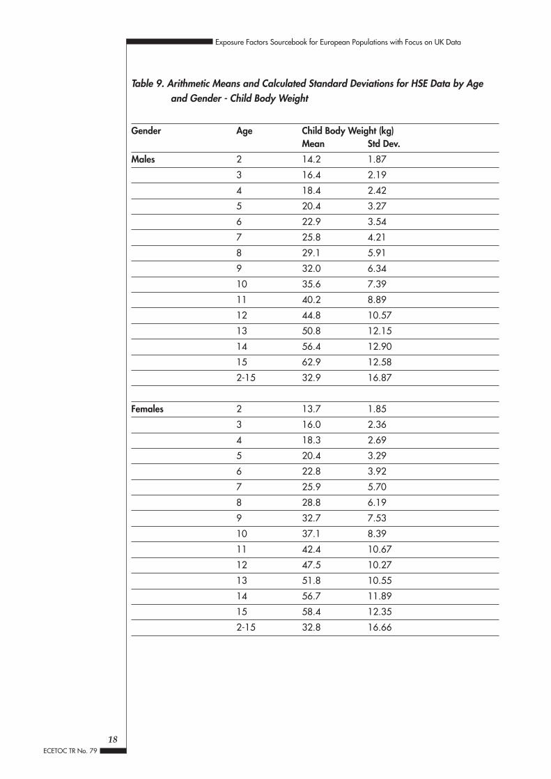
Table 9. Arithmetic Means and Calculated Standard Deviations for HSE Data by Ageand Gender - Child Body Weight

Gender Age Child Body Weight (kg)Mean Std Dev.

Males 2 14.2 1.87

3 16.4 2.19

4 18.4 2.42

5 20.4 3.27

6 22.9 3.54

7 25.8 4.21

8 29.1 5.91

9 32.0 6.34

10 35.6 7.39

11 40.2 8.89

12 44.8 10.57

13 50.8 12.15

14 56.4 12.90

15 62.9 12.58

2-15 32.9 16.87

Females 2 13.7 1.85

3 16.0 2.36

4 18.3 2.69

5 20.4 3.29

6 22.8 3.92

7 25.9 5.70

8 28.8 6.19

9 32.7 7.53

10 37.1 8.39

11 42.4 10.67

12 47.5 10.27

13 51.8 10.55

14 56.7 11.89

15 58.4 12.35

2-15 32.8 16.66

18


ECETOC TR No. 79

Table 10. Smoothed Percentiles of Body Weight (in kg) by Sex and Age: US ChildrenBirth to 36 Months (Source: USEPA, 1997 citation of Hamill et al, 1979)

Sex and Age Smoothed Percentilea

5th 10th 25th 50th 75th 90th 95thWeight in Kilograms

Male

Birth 2.54 2.78 3.00 3.27 3.64 3.82 4.15

1 Month 3.16 3.43 3.82 4.29 4.75 5.14 5.38

3 Months 4.43 4.78 5.32 5.98 6.56 7.14 7.37

6 Months 6.20 6.61 7.20 7.85 8.49 9.10 9.46

9 Months 7.52 7.95 8.56 9.18 9.88 10.49 10.93

12 Months 8.43 8.84 9.49 10.15 10.91 11.54 11.99

18 Months 9.59 9.92 10.67 11.47 12.31 13.05 13.44

24 Months 10.54 10.58 11.65 12.59 13.44 14.29 14.70

30 Months 11.44 11.80 12.63 13.67 14.51 15.47 15.97

36 Months 12.26 12.69 13.58 14.69 15.59 16.66 17.28

Female

Birth 2.36 2.58 2.93 3.23 3.52 3.64 3.81

1 Month 2.97 3.22 3.59 3.98 4.36 4.65 4.92

3 Months 4.18 4.47 4.88 5.40 5.90 6.39 6.74

6 Months 5.79 6.12 6.60 7.21 7.83 8.38 8.73

9 Months 7.00 7.34 7.89 8.56 9.24 9.83 10.17

12 Months 7.84 8.19 8.81 9.53 10.23 10.87 11.24

18 Months 8.92 9.30 10.04 10.82 11.55 12.30 12.76

24 Months 9.87 10.26 11.10 11.90 12.74 13.57 14.08

30 Months 10.78 11.21 12.11 12.93 13.93 14.81 15.35

36 Months 11.60 12.07 12.99 13.93 15.03 15.97 16.54

a Smoothed by cubic spline approximation

19


ECETOC TR No. 79

20


ECETOC TR No. 79

Tabl

e 11

. Bod

y W

eigh

t for

US

Mal

es, 6

Mon

ths

to 1

9 Ye

ars

of A

ge (S

ourc

e: U

SEPA

, 199

7 ci

tatio

n of

NC

HS,

198

7)

Age

Num

ber

ofM

ean

Std

Dev.

Perc

entil

ePe

rson

s(k

g)Ex

amin

ed5t

h10

th15

th25

th50

th75

th85

th90

th95

th6

- 11

mon

ths

179

9.4

1.3

7.5

7.6

8.2

8.6

9.4

10.1

10.7

10.9

11.4

1 ye

ar37

011

.81.

99.

610

.010

.310

.811

.712

.613

.113

.614

.42

year

s37

513

.61.

711

.111

.611

.812

.613

.514

.515

.215

.816

.53

year

s41

815

.72.

012

.913

.513

.914

.415

.416

.817

.417

.919

.14

year

s40

417

.82.

514

.115

.015

.316

.017

.619

.019

.920

.922

.25

year

s39

719

.83.

016

.016

.817

.117

.719

.421

.322

.923

.725

.46

year

s13

323

.04.

018

.619

.219

.820

.322

.024

.126

.428

.330

.17

year

s14

825

.13.

919

.720

.821

.222

.224

.826

.928

.229

.633

.98

year

s14

728

.26.

220

.422

.723

.624

.627

.529

.933

.035

.539

.19

year

s14

531

.16.

324

.025

.626

.027

.130

.233

.035

.438

.643

.110

yea

rs15

736

.47.

727

.228

.229

.631

.434

.839

.243

.546

.353

.411

yea

rs15

540

.310

.126

.828

.831

.833

.537

.346

.452

.057

.061

.012

yea

rs14

544

.210

.130

.732

.535

.437

.842

.548

.852

.658

.967

.513

yea

rs17

349

.912

.335

.437

.038

.340

.148

.456

.359

.864

.269

.914

yea

rs18

657

.111

.041

.044

.546

.449

.856

.463

.366

.168

.977

.015

yea

rs18

461

.011

.046

.249

.150

.654

.260

.164

.968

.772

.881

.316

yea

rs17

867

.112

.451

.454

.356

.157

.664

.473

.678

.182

.291

.217

yea

rs17

366

.711

.550

.753

.454

.858

.865

.872

.076

.882

.388

.918

yea

rs16

471

.112

.754

.156

.660

.361

.970

.476

.680

.083

.595

.319

yea

rs14

871

.711

.655

.957

.960

.563

.869

.577

.984

.386

.892

.1

21


ECETOC TR No. 79

Tabl

e 12

. Bod

y W

eigh

t for

US

Fem

ales

, 6 M

onth

s to

19

Year

s of

Age

(Sou

rce:

USE

PA, 1

997

cita

tion

of N

CH

S, 1

987)

Age

Num

ber

ofM

ean

Std

Dev.

Perc

entil

ePe

rson

s(k

g)Ex

amin

ed5t

h10

th15

th25

th50

th75

th85

th90

th95

th6

- 11

mon

ths

177

8.8

1.2

6.6

7.3

7.5

7.9

8.9

9.4

10.1

10.4

10.9

1 ye

ar33

610

.81.

48.

89.

19.

49.

910

.711

.712

.412

.713

.42

year

s33

613

.01.

510

.811

.211

.612

.012

.713

.814

.514

.915

.93

year

s36

614

.92.

111

.712

.312

.913

.414

.716

.117

.017

.418

.44

year

s39

617

.02.

413

.714

.314

.515

.216

.718

.419

.320

.221

.15

year

s36

419

.63.

315

.316

.116

.717

.219

.021

.222

.824

.726

.66

year

s13

522

.14.

017

.017

.818

.619

.321

.323

.826

.628

.929

.67

year

s15

724

.75.

019

.219

.519

.821

.423

.827

.128

.730

.334

.08

year

s12

327

.95.

721

.422

.323

.324

.427

.530

.231

.333

.236

.59

year

s14

931

.98.

422

.925

.025

.827

.029

.733

.639

.343

.348

.410

yea

rs13

636

.18.

025

.727

.529

.031

.034

.539

.544

.245

.849

.611

yea

rs14

041

.810

.929

.830

.331

.333

.940

.345

.851

.056

.660

.012

yea

rs14

746

.410

.132

.335

.036

.739

.145

.452

.658

.060

.564

.313

yea

rs16

250

.911

.835

.439

.040

.344

.149

.055

.260

.966

.476

.314

yea

rs17

854

.811

.140

.342

.843

.747

.453

.160

.365

.767

.675

.215

yea

rs14

555

.19.

844

.045

.146

.548

.253

.359

.662

.265

.576

.616

yea

rs17

058

.110

.144

.147

.348

.951

.355

.662

.568

.973

.376

.817

yea

rs13

459

.611

.444

.548

.950

.552

.258

.463

.468

.471

.681

.818

yea

rs17

059

.011

.145

.349

.550

.852

.856

.463

.066

.070

.178

.019

yea

rs15

860

.211

.048

.549

.751

.753

.957

.164

.470

.774

.878

.1

Table 13. Statistics for Maximum Likelihood Estimate Analysis of US Body Weight, 6Months to 20 Years (Source: Burmaster and Crouch, 1997)

Best Fit Parameters for Lognormal Distributions for Body Weight (kg)

Age Females Malesµ2* σ2* µ2* σ2*

6 months to 1 yr 2.16 0.145 2.23 0.129

1 to 2 yrs 2.38 0.129 2.46 0.120

2 to 3 yrs 2.56 0.113 2.60 0.118

3 to 4 yrs 2.69 0.136 2.74 0.115

4 to 5 yrs 2.82 0.135 2.86 0.133

5 to 6 yrs 2.93 0.164 2.98 0.140

6 to 7 yrs 3.08 0.173 3.11 0.146

7 to 8 yrs 3.19 0.176 3.21 0.152

8 to 9 yrs 3.31 0.157 3.32 0.180

9 to 10 yrs 3.43 0.216 3.42 0.167

10 to 11yrs 3.56 0.198 3.57 0.195

11 to 12 yrs 3.70 0.226 3.67 0.252

12 to 13 yrs 3.82 0.214 3.77 0.224

13 to 14 yrs 3.91 0.214 3.88 0.217

14 to 15 yrs 3.98 0.187 4.03 0.182

15 to 16 yrs 3.99 0.159 4.09 0.159

16 to 17 yrs 4.04 0.166 4.19 0.169

17 to 18 yrs 4.07 0.166 4.18 0.166

18 to 19 yrs 4.06 0.148 4.24 0.16

19 to 20 yrs 4.08 0.149 4.26 0.154

∗ µ2, σ2 correspond to the mean and standard deviation, respectively, of the lognormal distributionof body weight (kg) and are expressed in natural logarithms

22


ECETOC TR No. 79

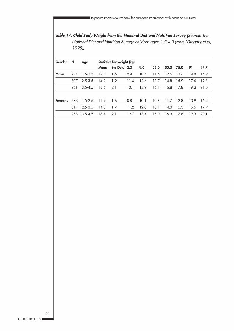
Table 14. Child Body Weight from the National Diet and Nutrition Survey (Source: TheNational Diet and Nutrition Survey: children aged 1.5-4.5 years (Gregory et al,1995))

Gender N Age Statistics for weight (kg)Mean Std Dev. 2.3 9.0 25.0 50.0 75.0 91 97.7

Males 294 1.5-2.5 12.6 1.6 9.4 10.4 11.6 12.6 13.6 14.8 15.9

307 2.5-3.5 14.9 1.9 11.6 12.6 13.7 14.8 15.9 17.6 19.3

251 3.5-4.5 16.6 2.1 13.1 13.9 15.1 16.8 17.8 19.3 21.0

Females 283 1.5-2.5 11.9 1.6 8.8 10.1 10.8 11.7 12.8 13.9 15.2

314 2.5-3.5 14.3 1.7 11.2 12.0 13.1 14.3 15.3 16.5 17.9

258 3.5-4.5 16.4 2.1 12.7 13.4 15.0 16.3 17.8 19.3 20.1

23


ECETOC TR No. 79

Table 15. Child Body Weight: Results of Monte Carlo Simulation of Estimated LognormalDistributions for HSE Data

Gender Age Statistics for weight (kg)Mean Std Dev. 5th 10th 50th 90th 95th

Males 2 14.2 2.0 11.3 11.9 14.0 16.9 17.8

3 16.5 2.2 13.1 13.7 16.4 19.3 20.5

4 18.5 2.5 14.6 15.5 18.3 21.9 22.8

5 20.2 3.2 15.1 16.1 19.9 24.4 25.6

6 22.9 3.8 17.3 18.4 22.6 27.7 29.5

7 25.9 4.1 19.9 21.0 25.5 31.5 33.5

8 29.3 6.1 20.6 22.0 28.8 37.2 40.1

9 31.9 6.2 22.7 24.7 31.2 40.4 42.8

10 35.8 7.4 25.3 27.0 34.9 45.2 48.9

11 40.5 9.2 27.1 29.9 39.2 52.4 57.1

12 44.9 10.2 29.7 32.6 44.2 58.2 62.7

13 50.5 12.4 33.3 35.7 49.2 67.4 72.6

14 56.5 13.0 37.5 41.0 54.7 73.7 79.0

15 62.7 12.8 44.1 47.8 61.3 79.7 85.7

2-15 34.0 19.0 13.1 15.2 29.8 59.0 71.9

Females 2 13.7 1.9 10.8 11.4 13.5 16.2 17.0

3 15.9 2.3 12.4 13.1 15.7 18.9 20.0

4 18.3 2.7 14.2 15.0 18.2 21.8 22.7

5 20.3 3.3 15.2 16.2 20.1 24.6 26.0

6 23.0 4.0 17.1 18.2 22.6 28.2 30.4

7 25.9 5.8 17.4 19.1 25.0 33.6 35.8

8 28.6 6.6 19.1 20.8 27.9 37.3 40.2

9 32.6 7.9 21.8 23.4 31.6 42.8 46.1

10 37.2 8.4 25.1 27.3 36.4 48.1 52.2

11 42.8 10.9 27.4 30.4 41.3 56.8 63.1

12 47.6 10.0 33.1 35.5 46.8 60.5 64.5

13 50.9 10.5 36.9 39.6 50.9 66.5 71.2

14 56.8 11.8 40.20 42.6 55.7 72.0 77.6

15 58.8 12.2 40.50 43.7 57.7 74.6 81.0

2-15 33.0 16.8 13.45 16.0 29.2 54.8 64.7

24


ECETOC TR No. 79

Figure 6. English Child Body Weight (combined ages 2-15) - Comparison of GenderSpecific Probability Distributions for HSE Data and Lognormal Monte CarloSimulations

Figure 7. English Female Child Body Weight - Comparison of Age Specific Distributionsfor HSE Data and Lorgnormal Monte Carlo Simulation by Age

25


ECETOC TR No. 79

3.3 Skin Surface Area

3.3.1 Total skin surface area

SummaryFor populations in which both body weight and height are known, skin surface areacan be calculated using the USEPA bivariate equation specified in this section.Alternatively, when only body weight data are available, skin surface area can becalculated using either the equation of Costeff or Burmaster. The equation of Burmastermay give a better estimate of central tendency than that of Costeff, but overestimatesskin surface area at values above the median. Based upon mean English adult bodyweight and the equation of Burmaster, total skin surface area is estimated as 2.07 m2 formales and 1.76 m2 for females, with an average of 1.92 m2. Skin surface area varies byboth gender and age. Estimated distributions for several gender and age groups arepresented in Table 16. Central tendency, upper and lower limits should be generatedbased upon body weight data representative of the population of interest.

Relevant StudiesThe direct measurement of body surface area (e.g., by direct coating, triangulation, orsurface area integration) is difficult and time-consuming. Because of this difficulty,various formulae have been developed for estimating skin surface area. Typical equationsexpress skin surface area as a function of both height and body weight or of body weightalone (DuBois and DuBois, 1916; Boyd, 1935; Gehan and George, 1970; USEPA, 1989;Burmaster, 1998a; Costeff, 1966).

The bivariate formula developed by the USEPA (1989) is based upon the largest sampleset (N=401) and included observations for adults as well as children (although childrenrepresented the majority of the sample population) (Murray and Burmaster, 1992). TheEPA bivariate formula accounts for >99.6% of the total variation among surface areaobservations for the sample population (Murray and Burmaster, 1992). Its form is:

SA= a Hb Wc

Where SA= Surface Area (m2)H = Height (cm)W= Weight (kg)a = 0.0239b = 0.417c = 0.517

When both body weight and height data are available for individuals within a population,the bivariate EPA equation is appropriate to use for estimating skin surface area. In mostcases, however, body weight data are readily available but combined body weightand height data for a given individual are limited. Thus, the skin surface area equations

26


ECETOC TR No. 79

based upon body weight alone are more readily applied. The two formulae that estimateskin surface area as a function of body weight alone are:

Equation 1: SA = (4W + 7)/(W+90)where SA = Surface Area (m2)W = Weight (kg)

Source: Costeff, 1966 in USEPA, 1997, based upon 220 observations of children

and

Equation 2: SA = a * BWc or ln SA = ln a + c ln BWwhere SA = Skin Surface AreaBW = Body Weightand: ln a = -2.2781, c = 0.6821 for all 401 people

ln a = -2.2752, c = 0.6868 for malesln a = -2.2678, c = 0.6754 for females

Source: Burmaster, 1998a, based upon 401 observations of adults and children

Given that body weight has been demonstrated to be lognormally distributed (Burmasterand Crouch, 1997), using the Burmaster (1998a) equation a distribution for skin surfacearea can be estimated as:

Equation 3: SA ~ exp [Normal[µSA, σSA]] where µSA = c * µBW + ln(a) and σSA = c * σBW

The equation of Costeff (1966) is a simpler formula, but skin surface area distributionscan be easily described using the Burmaster (1998) formula if lognormal body weightdistributions are known.

Cumulative skin surface area distributions were estimated using the equations ofboth Costeff and Burmaster for several age and gender categories (Table 16), using MonteCarlo simulations of body weight based upon the lognormal distribution parametersdefined in Tables 7 and 9. Both equations resulted in similar skin surface area distributionsfor children (Table 16, Figures 8-13).

For adults, the Burmaster equation resulted in higher estimates of skin surface area thanthe equation of Costeff (Table 16, Figures 14-16). This is not unexpected based uponprevious assessments of both equations. Both equations have been demonstrated toperform similarly to the bivariate EPA equation for adults, although the Costeff equationslightly underestimated adult male skin surface area (Costeff: mean and median both= 1.89 m2, USEPA bivariate: mean=1.97 m2 and median = 1.96 m2) and the Burmaster(1998a) equation was found to overpredict skin surface area above its median (Murrayand Burmaster, 1992; Burmaster, (1998a). If this same trend applies to the UK data, adultskin surface area obtained using the Burmaster (1998a) equation may be a better measureof central values, but values calculated using the Costeff (1966) equation are likely morerepresentative of upper limits. Given the relatively large difference in upper limits (100th

27


ECETOC TR No. 79

percentiles: Costeff 2.49, Burmaster: 3.12; 95th percentiles: Costeff: 2.19, Burmaster 2.51)but smaller difference in values at or below the median (50th percentile: Costeff =1.91, Burmaster: 2.06), it may be more appropriate to use the equation of Costeff togenerate skin surface area distributions for adults. For cases in which only a single centralestimate is needed, the equation of Burmaster should be used.

The correlation between skin surface area and body weight should be relatively consistentacross populations. Thus, skin surface area estimates for a given population can be madeusing the above equations and representative body weight data.

Using mean body weights of 80.0 kg for male and 67.3 kg for female adults (Table 1)and the equation of Burmaster (1998a), resulting skin surface areas are 2.07 m2 for malesand 1.76 m2 for females, with an average of 1.92 m2 for both genders. This is slightlygreater than the values of 1.93 m2 and 1.69 m2 for males and females and average of1.8 m2 suggested in the AIHC EFS (AIHC, 1994). The AIHC estimates are based uponthe bivariate EPA equation and less recent, lower values for body weight. Ninety-fifthpercentiles reported in the AIHC EFS were 2.28 and 2.09 m2 for male and female adults,respectively.

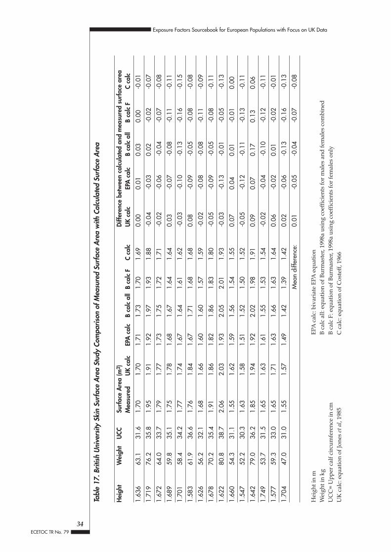
British University study:An equation is also available for a study of skin surface area performed at the Universityof Technology, Loughborough, UK (Jones et al, 1985). The sample population consistedof fifteen females aged 17-39 years, thirteen of whom were university students (nationalitynot specified). The individuals represented a variety of body sizes and shapes. Theresulting equation expressed skin surface area as a function of body weight and uppercalf circumference:

SA = 0.327 + 0.0071a + 0.0292bwhere SA = Surface Area (m2)

a = Body Weight (kg)b = Upper Calf Circumference (cm)

While both body weight and calf circumference are relatively easy to obtain, data oncalf circumference are extremely limited. In addition, the study population was notrepresentative of the general population. A comparison of the 15 measured surface areavalues and estimated surface area values by the equations of Jones, EPA, Costeff, andBurmaster for the general population and females specifically, is provided in Table 17.

3.3.2 Surface area of specific body parts

SummaryBased upon specific exposure scenarios, the expected fraction of skin exposed can beestimated using the body part specific fractions of total skin surface area provided inTable 18. Total skin surface area, estimated as specified in the previous section, can thenbe multiplied by the fraction exposed.

28


ECETOC TR No. 79

Relevant StudiesFor most typical dermal exposure scenarios, a portion of the body is exposed rather thanthe entire skin surface. Thus, estimates of surface area for specific body parts may bemore useful than estimates of total surface area.

The fraction of total skin surface area represented by individual body parts is presentedby age in Table 19. These averages are based upon US data of extremely small samplesize (N=1-5 for each yearly category between ages 1-18). Although limited, these datademonstrate how the fraction of total surface area associated with a given part varieswith age, particularly for the head and legs. The head area represents a larger proportionof total surface area for children, whereas the legs represent a larger percentage oftotal surface area for adults.

Mean proportions for children and adults from the EPA study and a recent review ofsurface area data (Ihme, 1994) are presented in Table 18. The mean values between thetwo studies are similar. More detailed information for the US adult data (maximum andminimum percentages by body part) is presented in Table 20.

Exposed skin surface area can be estimated by multiplying the total skin surface areapoint values or distributions by a constant value representing the fraction of skin thatis exposed. The fraction of exposed skin surface will depend upon climate and otheraspects specific to a given exposure scenario, such as type of activity. Suggested defaultsto use for some exposure scenarios are listed in Table 21 (USEPA, 1997). For hot climates,such as the Mediterranean regions, it may be typical for legs, arms, hands and feet tobe exposed. Based upon the Table 18 data, this scenario results in ~50% (children) to60% (adults) exposed surface area (65-70% if head area is also considered exposed).

If the fraction of skin that is exposed is expected to vary significantly over the exposureperiod, interpolation may be appropriate. For example, in a scenario with equal amountsof time expected at a low exposure (hands only) and high exposure (legs, arms, handsand feet), a mean value for fraction exposed can be used. Alternatively, if high exposurewould be expected for 3/4 of the exposure period and low exposure for 1/4, a weightedaverage can be taken. If a range of exposures are expected to occur, ex. hands, legs, arms,feet alone or in any combination of two or more, a uniform distribution between thelowest exposure fraction and highest exposure fraction may be more appropriate.

Examples of exposed skin surface area estimation for two exposure scenarios, one witha constant fraction of exposed skin and one with both high and low exposed area, areprovided in Appendix A.

29


ECETOC TR No. 79

30


ECETOC TR No. 79

Tabl

e 16

. Ski

n Su

rfac

e A

rea

Dist

ribut

ions

bas

ed u

pon

Logn

orm

al B

ody

Wei

ght D

istri

butio

ns fr

om H

SE D

ata

(199

6 fo

r A

dult

Mal

es, 1

995-

1997

for

Child

ren)

Stat

istic

s an

d pe

rcen

tiles

for

tota

l ski

n su

rfac

e ar

ea in

m2

SA E

quat

ion

Adu

lt M

ales

Fem

ales

, 2 y

rsM

ales

, 2 y

rsFe

mal

es, 1

0 yr

sM

ales

, 10

yrs

Cost

eff

Burm

aste

rCo

stef

fBu

rmas

ter

Cost

eff

Burm

aste

rCo

stef

fBu

rmas

ter

Cost

eff

Burm

aste

r

Mea

n1.

912.

080.

590.

600.

620.

641.

201.

171.

191.

12St

d D

ev.

0.17

0.25

0.06

0.05

0.06

0.06

0.18

0.18

0.16

0.17

Perc

entil

es:

01.

421.

450.

440.

460.

450.

480.

660.

670.

650.

675

1.65

1.71

0.50

0.52

0.52

0.55

0.93

0.91

0.93

0.93

101.

691.

770.

520.

530.

540.

570.

980.

960.

980.

9815

1.73

1.82

0.53

0.55

0.55

0.58

1.02

0.99

1.02

1.02

201.

771.

870.

540.

560.

560.

591.

051.

021.

051.

0525

1.80

1.90

0.55

0.57

0.57

0.60

1.07

1.05

1.08

1.08

301.

831.

950.

560.

570.

580.

611.

111.

081.

101.

1035

1.85

1.98

0.57

0.58

0.59

0.62

1.12

1.09

1.12

1.13

401.

872.

010.

580.

590.

600.

621.

151.

111.

151.

1545

1.89

2.04

0.58

0.59

0.61

0.63

1.17

1.14

1.17

1.17

501.

912.

060.

590.

600.

610.

641.

191.

161.

191.

1955

1.93

2.09

0.60

0.61

0.62

0.64

1.21

1.18

1.20

1.21

601.

952.

120.

610.

620.

630.

651.

241.

201.

221.

2365

1.97

2.15

0.62

0.63

0.63

0.66

1.26

1.23

1.24

1.25

702.

002.

200.

620.

630.

640.

671.

291.

261.

271.

2875

2.02

2.23

0.64

0.64

0.65

0.67

1.32

1.29

1.29

1.30

802.

052.

280.

650.

650.

660.

681.

361.

321.

321.

3385

2.09

2.35

0.65

0.66

0.68

0.70

1.39

1.36

1.36

1.37

902.

132.

410.

670.

680.

690.

711.

431.

401.

391.

4195

2.19

2.51

0.70

0.70

0.72

0.74

1.51

1.49

1.45

1.48

100

2.49

3.12

0.81

0.80

0.84

0.85

1.75

1.77

1.83

1.95

Figure 8. Monte Carlo Simulation of Skin Surface Area (m2) for Female Children 2 Yearsof Age, Calculated Using the Equation of Costeff

Figure 9. Monte Carlo Simulation of Skin Surface Area (m2) for Female Children 2 Yearsof Age, Calculated Using the Equation of Burmaster

Figure 10. Monte Carlo Simulation of Skin Surface Area (m2) for Male Children 2 Yearsof Age, Calculated Using the Equation of Costeff

31


ECETOC TR No. 79

Figure 11. Monte Carlo Simulation of Skin Surface Area (m2) for Male Children 2 Yearsof Age, Calculated Using the Equation of Burmaster

Figure 12. Comparison of Skin Surface Area Probability Distributions Generated Usingthe Equations of Costeff and Burmaster and Gender-Specific Lognormal BodyWeight Distributions for 2 Year Olds

Figure 13. Comparison of Skin Surface Area Probability Distributions Generated Usingthe Equations of Costeff and Burmaster and Gender-Specific Lognormal BodyWeight Distributions for 10 Year Olds

32


ECETOC TR No. 79

Figure 14. Monte Carlo Simulation of Adult Male Skin Surface Area Using CosteffEquation

Figure 15. Monte Carlo Simulation of Adult Male Skin Surface Area Using BurmasterEquation

Figure 16. Adult Male Skin Surface Area: Comparison of Probability DistributionsSimulated Using the Equations of Costeff and Burmaster

33


ECETOC TR No. 79

34


ECETOC TR No. 79

Tabl

e 17

. Brit

ish

Uni

vers

ity S

kin

Surf

ace

Are

a St

udy

Com

paris

on o

f Mea

sure

d Su

rfac

e A

rea

with

Cal

cula

ted

Surf

ace

Are

a

Hei

ght

Wei

ght

UCC

Surf

ace

Are

a (m

2 )Di

ffere

nce

betw

een

calc

ulat

ed a

nd m

easu

red

surf

ace

area

Mea

sure

dU

K ca

lcEP

A c

alc

B ca

lc a

llB

calc

FC

calc

UK

calc

EPA

cal

cB

calc

all

B ca

lc F

C ca

lc

1.63

663

.131

.61.

701.

701.

711.

731.

701.

690.

000.

010.

030.

00-0

.01

1.71

976

.235

.81.

951.

911.

921.

971.

931.

88-0

.04

-0.0

30.

02-0

.02

-0.0

7

1.67

264

.033

.71.

791.

771.

731.

751.

721.

71-0

.02

-0.0

6-0

.04

-0.0

7-0

.08

1.68

959

.835

.11.

751.

781.

681.

671.

641.

640.

03-0

.07

-0.0

8-0

.11

-0.1

1

1.70

158

.434

.21.

771.

741.

671.

641.

611.

62-0

.03

-0.1

0-0

.13

-0.1

6-0

.15

1.58

361

.936

.61.

761.

841.

671.

711.

681.

680.

08-0

.09

-0.0

5-0

.08

-0.0

8

1.62

656

.232

.11.

681.

661.

601.

601.

571.

59-0

.02

-0.0

8-0

.08

-0.1

1-0

.09

1.67

870

.235

.41.

911.

861.

821.

861.

831.

80-0

.05

-0.0

9-0

.05

-0.0

8-0

.11

1.62

280

.838

.72.

062.

031.

932.

052.

011.

93-0

.03

-0.1

3-0

.01

-0.0

5-0

.13

1.66

054

.331

.11.

551.

621.

591.

561.

541.

550.

070.

040.

01-0

.01

0.00

1.54

752

.230

.31.

631.

581.

511.

521.

501.

52-0

.05

-0.1

2-0

.11

-0.1

3-0

.11

1.64

279

.036

.21.

851.

941.

922.

021.

981.

910.

090.

070.

170.

130.

06

1.74

953

.731

.51.

651.

631.

611.

551.

531.

54-0

.02

-0.0

4-0

.10

-0.1

2-0

.11

1.57

759

.333

.01.

651.

711.

631.

661.

631.

640.

06-0

.02

0.01

-0.0

2-0

.01

1.70

447

.031

.01.

551.

571.

491.

421.

391.

420.

02-0

.06

-0.1

3-0

.16

-0.1

3

Mea

n di

ffere

nce:

0.01

-0.0

5-0

.04

-0.0

7-0

.08

Hei

ght i

n m

EPA

calc

: biv

aria

te E

PAeq

uatio

nW

eigh

t in

kgB

calc

all:

equ

atio

n of

Bur

mas

ter,

1998

a us

ing

coef

fici

ents

for

mal

es a

nd fe

mal

es c

ombi

ned

UC

C=

Upp

er c

alf c

ircu

mfe

renc

e in

cm

B ca

lc F

: equ

atio

n of

Bur

mas

ter,

1998

a us

ing

coef

fici

ents

for

fem

ales

onl

yU

K c

alc:

equ

atio

n of

Jone

s et

al,

1985

C c

alc:

equ

atio

n of

Cos

teff

, 196

6

Table 18. Percentage of Total Body Surface Area by Body Part

Body Part Source: Ihme, 1994 Source: USEPA, 1997Children1 Adults2 Children3 Adults4 Adults4

(min - max) (min - max) N (M:F)

Head 13 9 13 (9 - 18) 7 (6 - 11) 89 (32:57)

Neck 2 2

Trunk 34 (30 - 39) 35 (30 - 42) 89 (32:57)Arms 13 (12 - 16) 14 (12-16) 45 (32:13)

Lower arms 6 6 6 (5 - 6) 6 (6:0)Upper arms 8 8 7 (7 - 8) 6 (6:0)

Hands 5 5 5 (5 - 6) 5 (4 - 7) 44 (32:12)Legs 27 (18 - 32) 32 (26 - 35) 45 (32:13)

Thighs 19 (15 - 22) 45 (32:13)Lower legs 11 14 13 (11 - 16) 45 (32:13)

Feet 7 7 7 (6 - 8) 7 (6 - 8) 45 (32:13)

1 Ages 4 - < 10 years, N not provided2 Ages 20 - < 75 years, N not provided3 Average of the mean values for children aged < 1 - 14 year olds, N=19 (8 males:11 females)4 Average of the mean values for males and females

Table 19. Mean Percentage of Total Body Surface Area by Body Part by Age (Source:USEPA, 1997)

Age N (M:F) Head Trunk Hands Arms Legs Feet

< 1 2 (2:0) 18.2 35.7 5.3 13.7 20.6 6.5

1 < 2 2 (1:1) 16.5 35.5 5.7 13.0 23.1 6.3

2 < 3 1 (1:0) 14.2 38.5 5.3 11.8 23.2 7.1

3 < 4 5 (0:5) 13.6 31.9 6.1 14.4 26.8 7.2

4 < 5 4 (1:3) 13.8 31.5 5.7 14.0 27.8 7.3

6 < 7 1 (1:0) 13.1 35.1 4.7 13.1 27.1 6.9

9 < 10 2 (0:2) 12.0 34.2 5.3 12.3 28.7 7.6

12 < 13 1 (1:0) 8.7 34.7 5.4 13.7 30.5 7.0

13 < 14 1 (1:0) 10.0 32.7 5.1 12.1 32.0 8.0

16 < 17 1 (1:0) 8.0 32.7 5.7 13.1 33.6 6.9

17 < 18 1 (1:0) 7.6 31.7 5.1 17.5 30.8 7.3

Adult Males Note 1 7.8 35.9 5.2 14.1 31.2 7.0

Adult Females Note 1 7.1 34.8 5.1 14.0 32.4 6.5

Average for ages 1 - 14 13.3 34.4 5.4 13.1 26.6 7.1

Note 1 varies by body part, see N in Table 18

35


ECETOC TR No. 79

Tabl

e 20

. Add

ition

al D

etai

l of P

erce

ntag

e To

tal B

ody

Surf

ace

Are

a by

Bod

y Pa

rt fo

r A

dults

(Sou

rce:

USE

PA, 1

997)

Body

Par

tA

dult

Mal

esA

dult

Fem

ales

NM

ean

Std

Dev.

Min

Max

NM

ean

Std.

Dev.

Min

Max

Hea

d32

7.8

16.

111

577.

10.

65.

68.

1

Trun

k32

35.9

2.1

30.5

4157

34.8

1.9

32.8

41.7

Upp

er e

xtre

miti

es48

18.8

1.1

16.4

2157

17.9

0.9

15.6

19.9

Arm

s32

14.1

0.9

12.5

1613

140.

612

.414

.8U

pper

arm

s6

7.4

0.5

6.7

8.1

Fore

arm

s6

5.9

0.3

5.4

6.3

Han

ds32

5.2

0.5

4.6

712

5.1

0.3

4.4

5.4

Low

er e

xtre

miti

es48

37.5

1.9

33.3

4157

40.3

1.6

3643

.2Le

gs32

31.2

1.6

26.1

3313

32.4

1.6

29.8

35.5

Thig

hs32

18.4

1.2

15.2

2013

19.5

1.1

1821

.7Lo

wer

legs

3212

.81

1116

1312

.81.

011

.414

.9Fe

et32

70.

56

7.9

136.

50.

36

7

36


ECETOC TR No. 79

Table 21. Percentage of Total Surface Area that is Exposed for Various ExposureScenarios (Source: USEPA, 1997)

Scenario USEPA Recommendationsfor Percentage Exposed

Swimming and bathing 75 - 100

Adult outdoor exposure(only head and hands exposed) 10

Adult outdoor exposure(head, hands, forearms and lower legs exposed) 25

Moderate climate, winter 5

Moderate climate, spring and fall 10

Moderate climate, summer 25

3.4 Life Expectancy

SummaryThe average life expectancy of a UK child born in 1998 is 78 years. Life expectanciesfor European countries are found in Table 22.

Relevant StudiesRecent statistics on life expectancy for England are provided by gender in Tables 23 and24. Data indicate that life expectancy has been increasing over the last 25 years and thatmales have a shorter life expectancy than females. Average life expectancy for a childborn in England in 1996 is approximately 77 years (74.6 years for a male, 79.7 yearsfor a female); values for a child born in 1998 in the UK are similar (Table 22). Lifeexpectancies for children born in 1998 are reported for European countries in Table 22(WHO, 1999b). The UK value of 78 years is slightly greater than the value of 70 yearscommonly used for risk assessments and the value of 75 years recommended in the EFHbased upon US data for 1993 (USEPA, 1997).

37


ECETOC TR No. 79

Table 22. Average Life Expectancy at Birth in 1998, European Countries (Source: WHO,1999b)

Country Life Expectancy (years)M F M + F Average

Albania 70 76 73Armenia 67 74 71Austria 74 80 77Azerbaijan 66 74 70Belarus 62 74 68Belgium 74 81 78Bosnia and Herzegovina 71 76 74Bulgaria 68 75 72Croatia 69 77 73Czech Republic 70 77 74Denmark 73 78 76Estonia 63 75 69Finland 73 81 77France 74 82 78Georgia 69 77 73Germany 74 80 77Greece 76 81 79Hungary 67 75 71Iceland 77 81 79Ireland 74 79 77Israel 76 80 78Italy 75 81 78Kazakhstan 63 72 68Kyrgyzstan 63 72 68Latvia 62 74 68Lithuania 64 76 70Luxembourg 73 80 77Malta 75 79 77Netherlands 75 81 78Norway 75 81 78Poland 68 77 73Portugal 72 79 76Republic of Moldova 64 72 68Romania 66 74 70Russian Federation 61 73 67Slovakia 69 77 73Slovenia 71 78 75Spain 75 82 79Sweden 76 81 79Switzerland 75 82 79Tajikistan 64 70 67The Former Yugoslav Republic of Macedonia 71 75 73Turkey 67 72 70Turkmenistan 62 69 66Ukraine 64 74 69United Kingdom 75 80 78Uzbekistan 64 71 68Yugoslavia 70 75 73

38


ECETOC TR No. 79

Table 23. Male Expectation of Life at Birth (in 1996) and from Selected Ages in England(Source: UK Government Actuary’s Department, 1998,© Crown Copyright,used with permission)

Age (in years) 1982 1992 1993 1994 1995 1996

Birth (0) 71.3 73.7 74 74.1 74.4 74.6

5 67.3 69.3 69.6 69.7 70 70.2

20 52.7 54.6 54.9 55 55.3 55.5

30 43.1 45 45.3 45.5 45.7 45.9

50 24.5 26.3 26.6 26.7 27 27.1

60 16.5 18 18.2 18.3 18.5 18.7

70 10.2 11.2 11.4 11.4 11.6 11.7

80 5.8 6.4 6.5 6.6 6.6 6.7

Table 24. Female Expectation of Life at Birth (in 1996) and from Selected Ages inEngland (Source: UK Government Actuary's Department, 1998, © Crowncopyright, used with permission)

Age (in years) 1982 1992 1993 1994 1995 1996

Birth (0) 77.3 79.1 79.3 79.4 79.6 79.7

5 73.1 74.6 74.9 74.9 75.1 75.2

20 58.3 59.8 60.0 60.1 60.3 60.3

30 48.5 50.0 50.2 50.3 50.5 50.5

50 29.6 30.9 31.1 31.2 31.4 31.4

60 21.0 22.1 22.3 22.4 22.5 22.6

70 13.5 14.5 14.6 14.6 14.7 14.7

80 7.6 8.4 8.5 8.5 8.6 8.6

39


ECETOC TR No. 79

4. TIME-ACTIVITY PATTERNS

4.1 General Observations on Time-Activity Data

A number of studies have been performed that are related to time budgets of variousEuropean populations (Gershuny, 1985). Data are rarely published in a form that is usefulfor exposure assessment. In addition, data specifically for children were not identified.The parameters of most interest for exposure assessment are those associated withlocations where the greatest amount of time is spent (i.e., hours at work, home) or thoseassociated with specific activities where exposure potential may be greater (i.e., fieldsports, gardening, bathing). Also, time spent indoors vs. outdoors at each of the mainlocations is of importance. The raw data for several British surveys are available throughthe University of Essex data archives (http://dawww.essex.ac.uk). Data sets can bepurchased or specific analyses can be requested for a fee. The original data for somesurveys may be recorded in sufficient detail to produce the types of information neededfor exposure assessment.

4.2 Weekly Work Hours

SummaryAn average of 38-work hours/week is reported by the spring 1998 UK Labour ForceSurvey (Table 25). Distributions are provided in Table 26. These values represent hoursworked per week; additional time spent at the work site during non-working periods,such as lunch, is not included. Less than 4% of the surveyed population worked >60hours/week. The Labour Force Survey results include both full-time and part-timeworkers. An average value of 44 hours/week is probably more representative of full-time workers. Data were not identified for the portion of time spent working in a year.Based upon the assumption of 6 weeks for combined vacation and leave, an estimate of ~230 work days/year (46 weeks at 5 days/week) is obtained.

Relevant StudiesAverage weekly hours at work for the UK are provided in Table 25 for years between1994 - 1998. These values represent “hours worked per person per week.” They includeovertime (paid and unpaid), but do not include lunch periods (which may be spent atthe work locale). The weekly averages have remained relatively constant over the 1994 -1998 period. These data indicate that typical values for weekly hours at workare 38 hours/week for both males and females, 44 hours/week for males, and 31 hours/week for females. A distribution for hourly work hours is presented inTable 26. These values include both full- and part-time workers. Data from the OECDLabour Force Statistics for 1996 indicate that 8% of males and 45% of females employedin the UK worked part-time (Table 27). Thus, the male value is a better estimate of weeklywork hours for full-time workers. The available data are not sufficient to estimate amean value for full-time workers only. Excluding the lower 8% of responses, the medianvalue for weekly work hours for males still falls in the 31 - 45 hours/week range (thedistribution for all male responses is 9% in the < 5 - 30 hours/week range, 52% in the

40


ECETOC TR No. 79

31 - 45 range, and 39% in the 46 - > 60 range). Results of a 1983/84 time budget survey(Gershuny, 1985) yield similar weekly work hours for full-time employees(42.6 hours/week for full-time male workers, 38.6 hours/week for full-time femaleworkers).

Time budget data for a number of European countries were analysed by Gershuny (1995).A model was developed to estimate the effect of gender, employment status, age andfamily status and country on the minutes per day spent in each of several activities. Thecategories used were: “paid work” - includes hours working at home for pay andcommuting time; “all domestic unpaid work” - includes core domestic work and otherdomestic work; “out-of-home leisure - all leisure activities not performed at home; “TV,radio, etc.”; “at home leisure”; and “sleep” - includes personal care. The model predictionfor full-time UK workers is 44 hours/week, inclusive of commuting time.

These data do not provide specifics as to time spent at work at a place of employmentvs. paid work at home, or the amount of time at home spent in indoors vs. outdoorsactivity. In addition, details of the time budget surveys upon which they are based arenot specified. But they can be used as a rough estimate to indicate the relative amountof time spent at work, at home, or in away-from-home leisure activities by country.Gershuny’s model is presented in Table 28. This model is applied in Table 29 to estimatetime spent in full-time paid work (hours/week) by country (age and family statusand gender were not considered, just employment status and country).

Table 25. Average Usual Hours Worked per Person per Week (Source: UK Office forNational Statistics, 1999b, © Crown copyright, used with permission)

Gender 1994 1995 1996 1997 1998 Avg Std Dev.

M and F 38.2 38.3 38.1 38.8 38 38.28 0.31

M 44.4 44.4 44.2 44.1 44 44.22 0.18

F 30.6 30.7 30.6 30.8 30.8 30.70 0.10

41


ECETOC TR No. 79

Table 26. Cumulative Distribution for Usual Hours Worked per Person per Week -Number of People in Employment According to Number of Hours TheyUsually Work1(Source: UK Office for National Statistics2, 1999c, © Crowncopyright, used with permission)

Hours/week All Males Females

< 5 504 118 386

6 - 10 1089 251 839

11 - 15 1075 230 844

16 - 20 1671 300 1371

21 - 25 1237 232 1005

26 - 30 1157 257 901

31 - 45 12959 7593 5367

46 - 50 3274 2613 660

51 - 55 1300 1069 231

56 - 60 1206 1040 166

> 60 1127 963 164

1 Hours include overtime and exclude lunch breaks2 Values are presented as found at www.statistics.gov.uk/statbase

42


ECETOC TR No. 79

Table 27. Part-time Employment as % of Total Employment (Source: OECD, 1998a(Labour Force Statistics) and b (Employment Outlook), used with Permission)Basis: 1996 data

Country All F M

Austria 12.6 27.2 2.7

Belgium 14.0 30.5 3.0

Czech Republic 6.1 10.1 3.0

Denmark 21.5 34.5 10.8

Finland 11.6 15.3 8.3

France 16.0 29.5 5.3

Germany 16.5 33.6 3.8

Greece 5.3 9.0 3.3

Hungary 5.5 8.5 2.9

Iceland 27.9 47.4 11.0

Ireland 11.6 22.1 5.0

Italy 6.6 12.7 3.1

Luxembourg 7.7 18.4 1.5

Netherlands 36.5 66.1 16.1

Norway 26.6 45.9 10.2

Poland 10.6 13.4 8.3

Portugal 8.7 13.0 5.1

Spain 7.7 16.6 3.0

Sweden 23.6 39.0 9.3

Switzerland 27.4 52.2 8.3

Turkey 23.9 38.7 17.6

United Kingdom 24.6 44.8 8.1

EU-15 16.2 31.3 5.4

43


ECETOC TR No. 79

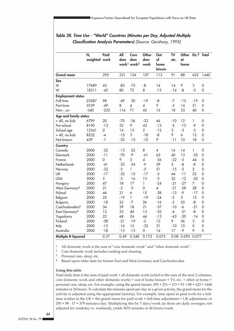
Table 28. Time Use - “World” Countries (Minutes per Day, Adjusted MultipleClassification Analysis Parameters) (Source: Gershuny, 1995)

N, Paid All Core Other Out TV Other Etc.3 Totalweighted work dom dom dom of etc. at

work1 work2 work home homeleisure

Grand mean 295 231 124 107 113 91 88 622 1440

SexM 17689 43 -83 -75 -8 14 14 9 3 0W 18311 -42 80 72 8 -13 -14 -8 -3 0

Employment statusFull-time 23587 98 -49 -30 -19 -8 -7 -15 -19 0Part-time 2539 -49 8 4 4 9 -3 14 21 0Non-, un- -340 -222 116 71 45 16 18 33 40 0

Age and family status< 40, no kids 6799 20 -70 -36 -33 46 -10 12 1 0Pre-school 8190 -13 52 9 43 -13 -5 -12 -9 0School age 12341 0 14 13 2 -12 3 -3 -3 0> 40, no kids 8232 -4 -15 3 -18 -8 9 6 12 0Not known 439 -1 -25 -15 -10 9 -11 10 18 0

CountryCanada 2000 -22 -13 -22 8 4 16 14 1 0Denmark 2000 -11 -70 -9 -61 63 40 13 -35 0France 2000 0 9 5 4 -26 -22 -5 44 0Netherlands 2000 -41 -33 -24 -9 29 5 -8 -8 0Norway 2000 -32 -5 1 -5 51 -15 -2 2 0UK 2000 -17 -32 -15 -17 -5 44 -11 22 0USA 2000 5 -3 -16 13 -3 32 -12 -20 0Hungary 2000 47 18 17 1 -24 -21 -27 7 0West Germany4 2000 21 -3 -3 0 4 -21 -28 28 0Poland 2000 46 21 6 15 -28 -13 -9 -17 0Belgium 2000 25 -19 1 -19 -24 -2 5 15 0Bulgaria 2000 -18 22 -7 26 -16 -2 25 -8 0Czechoslovakia4 2000 34 39 18 21 -37 -10 -6 -21 0East Germany4 2000 12 53 40 13 -32 -4 -21 -8 0Yugoslavia 2000 22 68 24 44 -13 -43 -20 -14 0Finland 2000 -38 -21 -19 -2 12 9 36 2 0Italy 2000 -15 -16 15 -32 31 -10 10 0 0Australia 2000 -18 -13 -13 0 14 17 -9 9 0

Multiple R-Squared 0.37 0.49 0.548 0.172 0.075 0.08 0.093 0.077

1 All domestic work is the sum of “core domestic work” and “other domestic work”.2 Core domestic work includes cooking and cleaning3 Personal care, sleep, etc.4 Based upon older data for former East and West Germany and Czechoslovakia

Using this tableTotal daily time is the sum of paid work + all domestic work (which is the sum of the next 2 columns,core domestic work and other domestic work) + out of home leisure + TV, etc. + other at home +personal care, sleep, etc. For example, using the grand means: 295 + 231 + 113 + 91 + 88 + 622 = 1440minutes or 24 hours. To calculate the minutes spent per day in a given activity, the grand mean for theactivity is adjusted using the appropriate factor(s). For example, time spent in paid work for a full-time worker in the UK = the grand mean for paid work + full-time adjustment + UK adjustment, or295 + 98 - 17 = 379 minutes/day. Multiplying this by 7 days/week (as these are daily averages, notadjusted for weekday vs. weekend), yields 2653 minutes or 44 hours/week.

44


ECETOC TR No. 79

Table 29. Estimated Weekly Work Hours for Full-time Workers by Country (Based uponthe Gershuny 1995 Time Use Model Presented in Table 28)

Country specific adjustments Adjusted data**Minutes/day Minutes/day Hours/week % of UK

Canada -22 371 43.3 99%

Denmark -11 382 44.6 102%

France 0 393 45.9 105%

Netherlands -41 352 41.1 94%

Norway -32 361 42.1 96%

UK -17 376 43.9 100%

USA 5 398 46.4 106%

Hungary 47 440 51.3 117%

West Germany* 21 414 48.3 110%

Poland 46 439 51.2 117%

Belgium 25 418 48.8 111%

Bulgaria -18 375 43.8 100%

Czechoslovakia* 34 427 49.8 114%

East Germany* 12 405 47.3 108%

Yugoslavia 22 415 48.4 110%

Finland -38 355 41.4 94%

Italy -15 378 44.1 101%

Australia -18 375 43.8 100%

* Model is based on older data for former East and West Germany and Czechoslovakia

** Adjusted data = base + full-time adjustment + country-specific adjustment

Paid work: = base time + full-time adjustment

= 295 + 98

= 393 minutes/day

45


ECETOC TR No. 79

4.3 Daily Hours at Home/Away

SummaryAmount of time spent at home depends upon work status. For full-time UK workers,averages of 15 hours/day at home, 9 hours/day away are estimated based upon 1984time budget data. For individuals not employed outside of the home, estimated averagesare 20.5 hours/day at home, 3.5 hours away. Of the total hours at home, approximately14 are spent indoors, 1 outdoors for full-time workers. For persons not employed outsidethe home, a split of 18.5 hours/day indoors, 2-hours/day outdoors is indicated. Thesevalues are based upon older data (from 1984), but consistent with other time budgetinformation. Country specific calculations based upon the model of Gershuny (1995)are presented in Table 30. The limitations of this model are discussed below. Datawere not available on the number of days away from home in travel each year.

Relevant StudiesThe UK numbers above are based upon the analysis of 1983/84 Economic and SocialResearch Council (ESRC) time budget data (Gershuny, 1985), and thus may not berepresentative of the current UK population. The ESRC survey is based upon a stratifiednational random sample of UK addresses. Time budget diaries were completed by 1600individuals >14 years of age. The range in average time spent at home is 14.9-21.3hours/day (Table 31). Results are provided for all ages combined. Similar values fordaily time indoors at home are reported by a more recent (1991) survey of 170 pregnantwomen residing in Avon, England (Farrow et al, 1997). Daily records of time indoorsat home were obtained for each expectant mother, the father, and the newborn infantfor approximately the last 6 months of pregnancy and first six months after birth. Mothers,fathers and young infants spent an average of 18.4, 14.7, and 19.3 hours/day indoors athome.

The model of Gershuny (1995) results in an intermediate estimate of time at home,approximately 17 hours/day, 7 hours/day away (Table 30). As specified in the previoussection, this model is based upon several time budget surveys that probably differed inmethodology, and were performed over a range of time. Study details were not provided.Time away from home was calculated as the sum of time at paid work and time in awayfrom home leisure. However, these data do not provide an adequate level of detail forestimating actual time at home. The “paid work” category included paid work performedfrom the home. The “time at home” estimate included time spent in domestic work suchas running errands outside of the home. The actual hours/day at home may not applybut the model results may be useful for estimating the proportion of time spent at homeby populations of other countries relative to the UK. Country specific model resultsrange from 16.9-17.8 hours/day at home, without adjusting for employment status.

The UK values reported are similar to median results from the US National HumanActivity Pattern Survey (USEPA, 1997). This study estimated that the US populationspends approximately 18.4 hours at home/day, 16.4 hours indoors and 2 hours outdoors.The NHAPS data are also broken down by categories such as age, gender, geographicregion (climate), and season, and cumulative distributions are provided. These data canbe consulted for additional estimates of time spent at home/away (USEPA, 1997).

46


ECETOC TR No. 79

Table 30. Estimated Weekly Hours Away from Home by Country (Based upon the TimeUse Model of Gershuny, 1995 Presented in Table 28)

Country-specific adjustments* Adjusted Work hours** Total time Total time % of UKaway leisure away at home

(minutes/day) (minutes/day) (minutes/day) (hours/day) (hours/day)

Canada 4 117 273 6.5 17.5 99.6%

Denmark 63 176 284 7.7 16.3 93.0%

France -26 87 295 6.4 17.6 100.4%

Netherlands 29 142 254 6.6 17.4 99.1%

Norway 51 164 263 7.1 16.9 96.1%

UK -5 108 278 6.4 17.6 100.0%

USA -3 110 300 6.8 17.2 97.7%

Hungary -24 89 342 7.2 16.8 95.7%

West Germany*** 4 117 316 7.2 16.8 95.5%

Poland -28 85 341 7.1 16.9 96.2%

Belgium -24 89 320 6.8 17.2 97.8%

Bulgaria -16 97 277 6.2 17.8 101.1%

Czechoslovakia***-37 76 329 6.8 17.3 98.2%

East Germany*** -32 81 307 6.5 17.5 99.8%

Yugoslavia -13 100 317 7.0 17.1 97.1%

Finland 12 125 257 6.4 17.6 100.4%

Italy 31 144 280 7.1 16.9 96.4%

Australia 14 127 277 6.7 17.3 98.3%

* Leisure away from home (base = 113 minutes/day)

** Not adjusted for employment status*** Model is based upon older data for former East and West Germany and Czechoslovakia

47


ECETOC TR No. 79

Tabl

e 31

. Sum

mar

y of

198

3/84

ESR

C Ti

me

Act

ivity

Dat

a (S

ourc

e: G

ersh

uny,

198

5)

Estim

ated

loca

tion

Ave

rage

hou

rs/d

ay s

pent

at e

ach

loca

tion

by e

mpl

oym

ent s

tatu

s an

d ge

nder

Ave

rage

of

% o

f day

Full-

time

Part

-tim

eU

nem

ploy

edN

onem

ploy

edca

tego

ries*

MF

MF

MF

MF

Hom

e-in

side

13.9

14.6

15.2

17.4

17.8

19.6

18.1

19.0

16.9

Hom

e-ou

tside

1.1

0.8

2.0

1.3

2.4

1.7

2.3

1.6

1.6

% o

f hom

e tim

e ou

tside

7.2%

5.4%

11.7

%7.

1%11

.8%

8.0%

11.1

%7.

7%8.

8%

Aw

ay-in

door

s1.

51.

92.

11.

92.

61.

61.

81.

91.

9A

way

-out

door

s0.

70.

50.

80.

70.

80.

70.

80.

70.

7W

ork

6.8

6.1

4.6

2.7

0.4

0.3

1.0

0.7

2.8

Tota

l Hom

e14

.915

.417

.218

.720

.221

.320

.420

.618

.678

%To

tal A

way

(not

wor

k)2.

22.

42.

82.

53.

42.

32.

62.

62.

611

%To

tal W

ork

6.8

6.1

4.6

2.7

0.4

0.3

1.0

0.7

2.8

12%

Tota

l Ind

oors

(inc

. wor

k)22

.122

.621

.921

.920

.821

.520

.921

.621

.790

%

Tota

l Out

door

s1.

81.

32.

82.

03.

22.

43.

02.

32.

410

%

Hom

e-in

side

cat

egor

ies

wer

e ch

ild c

are,

coo

king

, dre

ssin

g, e

atin

g, h

ouse

wor

k, r

adio

, rec

ords

, sle

epin

g, s

tudy

at h

ome,

talk

ing,

tv a

nd v

ideo

Hom

e-ou

tsid

e ca

tego

ries

wer

e D

IY(d

o it

your

self

) and

gar

deni

ngH

ome-

half

out

side

, hal

f ins

ide

cate

gori

es w

ere

hobb

ies,

gam

es, h

ome

ente

rtai

nmen

t, re

adin

g, w

ritin

g, r

elax

ing

Aw

ay-i

ndoo

rs c

ateg

orie

s w

ere

ente

rtai

ning

aw

ay, m

eetin

gs, p

ubs,

res

taur

ants

, rel

igio

n, s

hopp

ing,

thea

tre,

cin

ema,

mus

eum

Aw

ay-o

utdo

ors

cate

gori

es w

ere

play

ing

spor

t, w

alki

ng, w

atch

ing

spor

tA

way

-hal

f ind

oors

, hal

f out

door

s ca

tego

ries

wer

e do

mes

tic tr

avel

, err

ands

, lei

sure

trav

el

Wor

k w

as c

onsi

dere

d in

door

s

*N

umbe

r is

an

aver

age

acro

ss c

ateg

orie

s an

d no

t nec

essa

rily

rep

rese

ntat

ive

of th

e po

pula

tion

ave

rage

(whi

ch w

ould

wei

ght e

ach

cate

gory

by

its

perc

ent o

f the

tota

lpo

pula

tion)

48


ECETOC TR No. 79

4.4 Time Indoors/Outdoors

RecommendationsAverage daily values of 22 hours indoors, 2 hours outdoors are estimated for UK adults.

Relevant StudiesBased upon data from a 1983/84 ESRC time budget survey, estimated time indoorsis ~22 hours/day (Table 31 of previous section). These data are from 1984 and maynot be representative of the current population. The results, however, are consistent witha number of other studies. Ott (1988) indicated that time spent outdoors, including travel,in a number of European countries was 2-3 hours/day. Based upon US data, 21 hoursare spent indoors, 1.5 hours outdoors and 1.5 hours in travel per day (USEPA, 1997).Values of 22.3 hours indoors and 1.7 hours outdoors per day are recommended in theEFS (AIHC, 1994)

4.5 Daily School Hours

SummaryA value of 7 hours/day for 190 days per year is estimated for UK children, based uponinformation provided by the Department for Education and Employment. For secondaryschool children involved in extracurricular activities, a value of 8 hours/day may bemore representative. Children participating in after school or breakfast clubs spend moretime per day at school, but data are not available for typical starting or ending time ofthese activities.

Relevant StudiesInformation on typical patterns of school attendance was provided by the UK Departmentfor Education and Employment (1999). Typical hours for primary and secondary schoolsare 9:00 a.m. - 3:30 p.m., although arrival on school premises probably occurs around8:45 am. It is likely that several minutes are also spent on school premises after dismissal.Based upon 6.5 core hours/day and approximately 15 minutes before and after corehours, estimated time on school premises is 7 hours/school day.

A survey of weekly time for which teachers are present at school to supervise children(i.e., time spent in lessons, collective worship, assembly, registration, breaks andsupervision, but not the teachers’ lunch periods) is available for 8 primary schoolsand 10 secondary schools (Department of Education and Science, 1990). The weeklyhours do not include lunch periods. This survey reports total weekly hours of 26.4 - 30.0for primary schools and 28.3 - 30.8 for secondary schools. Dividing by five results in5.3 - 6.0 hours/day for primary schools and 5.7 - 6.2 hours/day for secondary schools.The sample size is extremely small, but values are consistent with the informationprovided for typical school hours. If lunch periods are included, daily hours are similarto those estimated above.

Children in secondary school may be involved in extracurricular activities, which typicallyend about 4:30 pm (one hour additional to the normal school hours). Thus, a total

49


ECETOC TR No. 79

time of 8 hours/day can be used for these children. No information was available forthe percentage of children participating in extracurricular activities or the frequency ofparticipation (i.e., how many days/week).

Some children may participate in after school or breakfast clubs, programmes designedfor children who need to arrive earlier or stay later than typical school hours. Althoughspecific data are not available, the Department for Education and Employment indicatedthat only a minority of children, perhaps 10%, participate in these clubs.

The minimum number of school days per year is 190 in the UK (Department of Educationand Science, 1990). Information provided by the Department for Education andEmployment (2000b) was used to estimate the actual number of school days per year.The department indicated that holidays consist of 6 weeks in summer, 2 weeks atChristmas, 2 weeks at Easter, and ~5 public holidays or teacher training days that occurduring the school year. Three additional “half-term” breaks of one week each are alsotypical. This results in ~14 weeks on holiday, 38 weeks at school per year. At 5 daysper school week, the resulting yearly estimate is 190 days, equivalent to the minimumnumber of days required in the UK. This estimate is based upon perfect attendance, andis thus very probably a conservative value for days at school.

4.6 School Time Indoors/Outdoors

SummaryUnder favourable weather conditions, approximately 2 hours/day may be spent outdoors,5 hours per day indoors. This value does not include extracurricular activities.

Relevant StudiesThe UK Department for Education and Employment (1999) indicated that the majorityof the school day is spent indoors. Periods that may be spent outdoors under favourableweather conditions include time between arrival on school premises and commencementof school day, after lunch recess, break time, physical education class, and time betweendismissal and departure from school premises. Excluding extracurricular activities, timebefore and after school was estimated as 15 minutes each for a total of 30 minutes.The Department for Education and Employment indicated that typical values for theother activities are: after lunch recess - 30 minutes; break time - 20 minutes; physicaleducation class-45 minutes. For a day in which all of these activities occur outdoors,~ 2 hours (125 minutes) is spent outside. For a typical school day of 7 hours, this resultsin ~5 hours indoors. For a child involved in extracurricular activities, the setting ofadditional time spent at school will depend upon the nature of the activity.

4.7 Outdoor Recreation

SummaryAn average daily value of 0.3 hours is estimated for 365 days/year for adults. Averagedaily values across gender and employment status ranged from 0.2-0.4 hours/day (Table32). These values represent population averages from the ESRC time budget survey

50


ECETOC TR No. 79

(Gershuny, 1985). For US population members who participate in outdoor recreationalactivity, a median of 2.5 hours has been reported for a day in which outdoor activitytook place (US data - cumulative distribution provided in Table 33; 95th and 99thpercentiles of 9.6 and 11.5 hours, respectively).

Relevant StudiesThe average daily value of 0.3 hours is based upon the 1983/84 ESRC time budget surveydata (Gershuny, 1985). Only categories estimated to represent away from home, outdoorleisure activities were used to develop this estimate (Table 32). Time allocated to homeleisure activities (indoors and outdoors) is already considered under hours per day athome. Away from home leisure activities associated with indoor settings (leisure travel,entertaining away from home, pubs, restaurant, theatre, cinema and visits to museums)were not considered because they are likely to be performed at different locations ondifferent days. All outdoor away from home leisure activities were assumed to takeplace at the same location each day.

Note, the values above are based upon total outdoor recreation time averaged overthe study period, and are representative of a long-term average. The averages includezero values for days in which no outdoor recreational activity was observed and foradults who did not participate at all in this type of activity. Under normal circumstances,outdoor recreational activity will take place for a longer period of daily time, but foronly a portion of days in a year. In addition, some adults will not participate in outdoorrecreation. Data were not available for the number of days per year that outdoor recreationoccurred or for the percent of the population that participated in outdoor recreation.

Results of the US NHAPS survey indicate that for individuals who reported outdoorrecreational activity, a 50th percentile of 2.5 hours/day was estimated (distributionprovided in Table 33). However, the number of occurrences per year of outdoor activitywere not reported. Only 253 of 9386 respondents (~3%) reported participating in outdoorrecreational activities during the survey period (USEPA, 1997).

For days in which outdoor recreation occurred, adults (aged 18-64 years) exhibitedhigher daily median times in outdoor recreation than children (age categories 1-4, 5-11 and 12-17 years) (Table 33). However, it is likely that the frequency (days/year) spentin outdoor recreation is greater for children, based upon typical age related behaviouralpatterns.

51


ECETOC TR No. 79

Table 32. 1983/84 ESRC Time Activity Data for Outdoor, Away from Home Recreation(Source: Gershuny, 1985)

Category Average minutes/day spent in activity by employment status and genderFull-time Part-time Unemployed Nonemployed AverageM F M F M F M F

Playing sport 10.5 2.6 12 3.3 10.8 2.9 8.1 5.5 7.0

Walking 8.4 4.3 7.7 4.5 7.8 16.3 15.4 7.6 9.0

Watching sport 1.6 1.1 0.04 3.3 2.4 0.0 1.0 0.4 1.2

SUM 20.5 8 19.74 11.1 21 19.2 24.5 13.5 17.2

SUM (hrs/day) 0.34 0.13 0.33 0.19 0.35 0.32 0.41 0.23 0.29

4.8 Shower Duration

SummaryData were not identified for European populations. An average of 7.7 minutes/day isreported for a survey of Australian households. The 95th percentile is 13.5 minutes/day.The distribution of Burmaster (1998b), based upon the Australian data, can be used toestimate shower duration.

Relevant StudiesUK or European specific data were not identified for this parameter. Available dataare from a survey of 2,500 Australian households (James and Knuiman; Burmaster,1998b). The mean showering time is 7.7 minutes/day. The mode, median and 95thpercentiles are 6.2, 7.2, and 13.5 minutes/day (Burmaster, 1998b). Burmaster (1998b)developed the following distribution for shower duration based upon these data:

Ts ~ exp[Normal(1.9705, 0.3864)]Where Ts = shower duration in minutes/day.

These data may not be representative of European customs. In the absence of Europeanspecific data, however, they are recommended for use. In addition, data from the USNational Human Activity Pattern Survey (NHAPS) on daily time spent bathing canbe consulted. The NHAPS data are available as a cumulative distribution, but dataare presented for "doers" only (survey participants who did not perform a given activityon the survey day are not included) (USEPA, 1997). The NHAPS data indicate that timespent in the shower or bathtub (minutes/bath) is generally greater for children thanadults. Median values are 15 minutes/bath for the general population but 20minutes/bath for children ≤ 11 years of age. Ninety-fifth percentiles are 35 minutes/bathfor the general population and 60 minutes/bath for children (USEPA, 1997).

52


ECETOC TR No. 79

4.9 Employment Tenure

SummaryAn employer tenure (time spent working for current employer) of 8 years is reportedas an average value for the UK, and 4.4 years as a median. Approximately 10% of thesurveyed UK population had an employer tenure of > 20 years (maximum not reported)and 19% under 1 year. Data for the UK and other countries are summarised in Table 34.

Relevant StudiesEmployment time can be tracked as occupational tenure or employer tenure (USEPA,1997). Occupational tenure represents the cumulative time a person has worked in hisor her current occupation, regardless of the number of employers, periods ofunemployment, or periods of employment in other occupations. Employer tenurerepresents the period of time a person has worked for his or her current employer.

OECD (1993) summarised information on “enterprise” tenure from surveys performedin a number of countries (Table 34). OECD indicates that survey designs varied acrosscountries, but that participants were typically asked how long they had been workingfor their present employer. Thus, these data are representative of employer tenure ratherthan occupational tenure.

The median and average enterprise tenure for European countries is greater than thoseof the US (Table 34). Data on occupational tenure for European countries were notidentified. A median US occupational tenure of 6.6 years was reported in the EFH (USEPA,1997). This value exceeds the median US enterprise (employer) tenure of3.0 years reported in Table 34. A median working tenure (number of years spent at aspecific job) of 4 years was reported in the AIHC EFS based upon US data, with a 95thpercentile of 25 years (AIHC, 1994).

53


ECETOC TR No. 79

Tabl

e 33

. Sta

tistic

s fo

r 24

-Hou

r Cu

mul

ativ

e N

umbe

r of

Min

utes

Spe

nt in

Out

door

Rec

reat

ion,

US

Data

(Sou

rce:

USE

PA, 1

997)

Cate

gory

Popu

latio

nN

Mea

nSt

d De

v.St

d Er

r.M

inM

axPe

rcen

tiles

Gro

up5

2550

7590

9598

99A

ll25

321

1.23

185.

4811

.661

514

4020

6016

530

048

057

467

069

0G

ende

rM

ale

140

231.

7820

7.41

17.5

295

1440

17.5

67.5

177

330

502.

560

069

073

5G

ende

rFe

mal

e11

218

3.67

150.

1514

.188

564

520

6015

025

538

052

558

563

0G

ende

rRe

fuse

d1

420

**

420

420

420

420

420

420

420

420

420

420

Age

(yea

rs)

*2

337.

520

1.53

142.

519

548

019

519

533

7.5

480

480

480

480

480

Age

(yea

rs)

1 - 4

1316

6.54

177.

0649

.109

1563

015

3013

018

037

063

063

063

0A

ge (y

ears

)5

- 11

2120

6.14

156.

1734

.078

3058

560

9016

524

536

057

458

558

5A

ge (y

ears

)12

- 17

2715

5.07

128.

2824

.687

546

55

6013

522

542

042

046

546

5A

ge (y

ears

)18

- 64

158

223.

6119

2.97

15.3

525

1440

3080

172.

531

050

558

569

069

0A

ge (y

ears

)>

6432

211.

0620

6.59

36.5

215

735

530

171

375

495

600

735

735

Empl

oym

ent

*60

177.

115

0.02

19.3

685

630

12.5

6014

7.5

230

395

519.

558

563

0Em

ploy

men

tFu

ll-tim

e10

421

0.74

153.

3715

.039

567

030

82.5

180

294

419

511

600

645

Empl

oym

ent

Part-

time

1920

5.26

204.

0446

.81

3069

030

6015

018

057

069

069

069

0Em

ploy

men

tN

ot E

mpl

oyed

6824

4.44

245.

0329

.715

514

4015

6017

9.5

375

525

690

735

1440

Empl

oym

ent

Refu

sed

218

7.5

10.6

077.

518

019

518

018

018

7.5

195

195

195

195

195

Educ

atio

n*

6417

6.73

145.

3218

.165

563

015

6015

2.5

225

370

465

585

630

Educ

atio

n<

Hig

h Sc

hool

2225

9.41

177.

9737

.943

560

030

105

247.

538

052

560

060

060

0Ed

ucat

ion

H.S

. Gra

duat

e59

238.

222

8.99

29.8

1215

1440

2090

175

310

511

670

690

1440

Educ

atio

n<

Col

lege

5421

8.09

172.

2123

.434

569

025

6517

2.5

345

460

550

570

690

Educ

atio

nC

olle

ge G

rad

3122

4.71

193.

0634

.675

2069

030

6015

032

550

564

569

069

0Ed

ucat

ion

Post

Gra

duat

e23

157.

6117

8.18

37.1

535

735

1050

8020

037

048

073

573

5C

ensu

s Re

gion

Nor

thea

st52

189.

616

0.88

22.3

15

690

3060

162.

523

1.5

370

574

670

690

Cen

sus

Regi

onM

idw

est

5421

2.09

228.

4131

.083

514

4020

6017

7.5

280

419

600

735

1440

Cen

sus

Regi

onSo

uth

8421

7.26

175.

2719

.123

564

515

62.5

150

347.

549

552

560

064

5C

ensu

s Re

gion

Wes

t63

220.

2917

9.71

22.6

4210

690

3075

165

280

545

585

690

690

Day

of W

eek

Wee

kday

129

197.

2119

5.32

17.1

975

1440

1560

150

275

465

525

670

735

Day

of W

eek

Wee

kend

124

225.

8117

4.26

15.6

495

690

2085

180

310

480

600

690

690

Seas

onW

inte

r31

196.

6116

5.52

29.7

285

585

560

165

280

440

550

585

585

Seas

onSp

ring

7519

8.85

161.

6718

.668

569

025

7518

027

046

554

567

069

0Se

ason

Sum

mer

102

228.

1610

4.18

20.2

175

1440

3075

179.

532

545

958

569

069

0Se

ason

Fall

4520

3.53

193.

8328

.895

573

520

6012

033

050

557

473

573

5

54


ECETOC TR No. 79

Tabl

e 34

. Dis

tribu

tion

of E

mpl

oym

ent b

y En

terp

rise

(Em

ploy

er) T

enur

e, 1

991

(Sou

rce:

OEC

D, 1

993)

Aus

tralia

Aus

triaa

Cana

daFi

nlan

dFr

ance

Ger

man

ydJa

pand

Net

herla

ndsd

Nor

way

eSp

aing

Switz

erla

ndU

KU

SAU

nwei

ghte

dav

erag

eh

Curr

ent t

enur

e (%

)To

tal

100.

010

0.0

100.

010

0.0

100.

010

0.0

100.

010

0.0

100.

010

0.0

100.

010

0.0

100.

010

0.0

Und

er 1

yea

r21

.413

.823

.511

.915

.712

.89.

824

.014

.9f

23.9

17.6

18.6

28.8

18.6

1 an

d un

der 2

yea

rs13

.220

.0c

12.8

10.7

10.3

16.1

c15

.511

.0f

7.7

11.7

12.4

11.6

2 an

d un

der 5

yea

rs25

.915

.2b

11.9

c24

.515

.617

.911

.5c

22.9

18.0

f14

.820

.723

.921

.3U

nder

5 y

ears

60.6

55.4

49.2

42.0

41.0

37.4

62.4

43.9

f46

.449

.954

.861

.750

.45

and

unde

r 10

year

s16

.232

.6b

15.2

16.7

16.2

17.8

19.7

11.4

19.7

14.0

16.8

16.1

11.7

16.0

10 a

nd u

nder

20

year

s15

.236

.7b

19.4

21.4

25.6

24.5

23.6

15.2

24.1

21.3

18.8

19.3

17.8

20.5

20 y

ears

and

ove

r8.

110

.012

.815

.816

.719

.311

.012

.318

.413

.89.

68.

813

.0U

nkno

wn

---

1.7

0.4

0.8

0.1

Ave

rage

tenu

re (y

ears

)A

ll pe

rson

s6.

8--

-7.

89.

010

.110

.410

.97.

09.

49.

88.

87.

96.

78.

7M

en7.

8--

-8.

99.

410

.612

.112

.58.

610

.210

.610

.49.

27.

59.

8W

omen

5.4

---

6.5

8.5

9.6

8.0

7.3

4.3

8.4

8.2

6.6

6.3

5.9

7.1

Med

ian

tenu

re (y

ears

)A

ll pe

rson

s3.

5--

-4.

15.

27.

57.

58.

23.

16.

56.

35.

04.

43.

05.

4M

en4.

1--

-4.

85.

87.

99.

510

.13.

97.

47.

57.

15.

33.

56.

4W

omen

2.9

---

3.3

4.9

7.0

5.0

4.8

2.0

5.8

3.3

3.6

3.7

2.7

4.1

a19

88e

1989

b1

and

unde

r 3

year

s, 3

and

und

er 1

0 ye

ars,

and

10

year

s an

d ov

erf

Und

er 2

1 m

onth

s, 2

1 an

d un

der 3

3 m

onth

s, 3

3 an

d un

der 5

7 m

onth

s, a

nd u

nder

57

mon

ths

c1

and

unde

r 3

year

s an

d 3

and

unde

r 5

year

sg

1992

d19

90h

The

unw

eigh

ted

aver

age

excl

udes

Aus

tria

55


ECETOC TR No. 79

4.10 Residential Tenure

SummaryA median value of 9 years is reported for either current or total residence time basedupon US data. Distributions of current residence time are provided in Table 35.Distributions of total residency time by gender and age are provided in Tables 36 and37. Total residence time by geographic region and housing category are provided inTables 38 and 39.

Relevant StudiesNo data were identified for the UK or Europe. In the absence of European specific data,US data were used. These data may not be representative of European populations.Residence time is reported as either total residence time (time between moving into andout of a residence) or current residence time (time since moving into the current residence).A distribution for current residence time based upon a 1991 sample of 93,000 UShouseholds is presented in Table 35. Results for total residence time, which must bemodelled, are available for two studies: Israeli and Nelson (1992) and Johnson and Capel(1992). Due to differences in modelling approach, the inclusion of age as a factor affectingresidence time, and the use of more recent data, the results of Johnson and Capel wereassessed to be more representative than those of Israeli and Nelson (AIHC, 1994).Distributions of total residency time by gender and age are provided in Tables 36and 37.

Results of the Israeli and Nelson study offer the advantage of being reported by householdtype (urban vs. rural, geographic region). Thus, the Israeli and Nelson results may bemore useful for application to specific European regions if these factors are assumedto affect population mobility in the same manner. Total residence time by geographicregion and housing category are provided in Tables 38 and 39.

Table 35. Distribution for Current Residential Tenure, US Data (Source: USEPA, 1997adaptation of U.S. Bureau of Census, 1993)

Years lived in current home Percent of total households0-4 26.345-9 29.0410-14 11.3915-19 10.0620-24 6.6924-33 8.5234-44 5.145-54 1.9>55 0.95Totala: 99.99a Total does not equal 100 due to rounding errors

56


ECETOC TR No. 79

Table 36. Residential Occupancy Period, US Data (Source: USEPA, 1997 citation ofJohnson and Capel, 1992)

Statistic Residential occupancy period (years)Both genders Males only Females onlyNa = 500,000 N = 244,274 N = 255,726

Mean 11.7 11.1 12.3

5th percentile 2 2 2









99.5th percentile 51 48 53



Second largest value 75 73 75

Largest value 87 73 87

a = Number of simulated persons

57


ECETOC TR No. 79

Table 37. Residential Occupancy Period by Age, US Data (Source: USEPA, 1997 citationof Johnson and Capel, 1992)

Current Age (years) Residential occupancy period (years)Mean Percentile

25 50 75 90 95 99

3 6.5 3 5 8 13 17 22

6 8.0 4 7 10 15 18 22

9 8.9 5 8 12 16 18 22

12 9.3 5 9 13 16 18 23

15 9.1 5 8 12 16 18 23

18 8.2 4 7 11 16 19 23

21 6.0 2 4 8 13 17 23

24 5.2 2 4 6 11 15 25

27 6.0 3 5 8 12 16 27

30 7.3 3 6 9 14 19 32

33 8.7 4 7 11 17 23 39

36 10.4 5 8 13 21 28 47

39 12.0 5 9 15 24 31 48

42 13.5 6 11 18 27 35 49

45 15.3 7 13 20 31 38 52

48 16.6 8 14 22 32 39 52

51 17.4 9 15 24 33 39 50

54 18.3 9 16 25 34 40 50

57 19.1 10 17 26 35 41 51

60 19.7 11 18 27 35 40 51

63 20.2 11 19 27 36 41 51

66 20.7 12 20 28 36 41 50

69 21.2 12 20 29 37 42 50

72 21.6 13 20 29 37 43 53

75 21.5 13 20 29 38 43 53

78 21.4 12 19 29 38 44 53

81 21.2 11 20 29 39 45 55

84 20.3 11 19 28 37 44 56

87 20.6 10 18 29 39 46 57

90 18.9 8 15 27 40 47 56

All ages 11.7 4 9 16 26 33 47

58


ECETOC TR No. 79

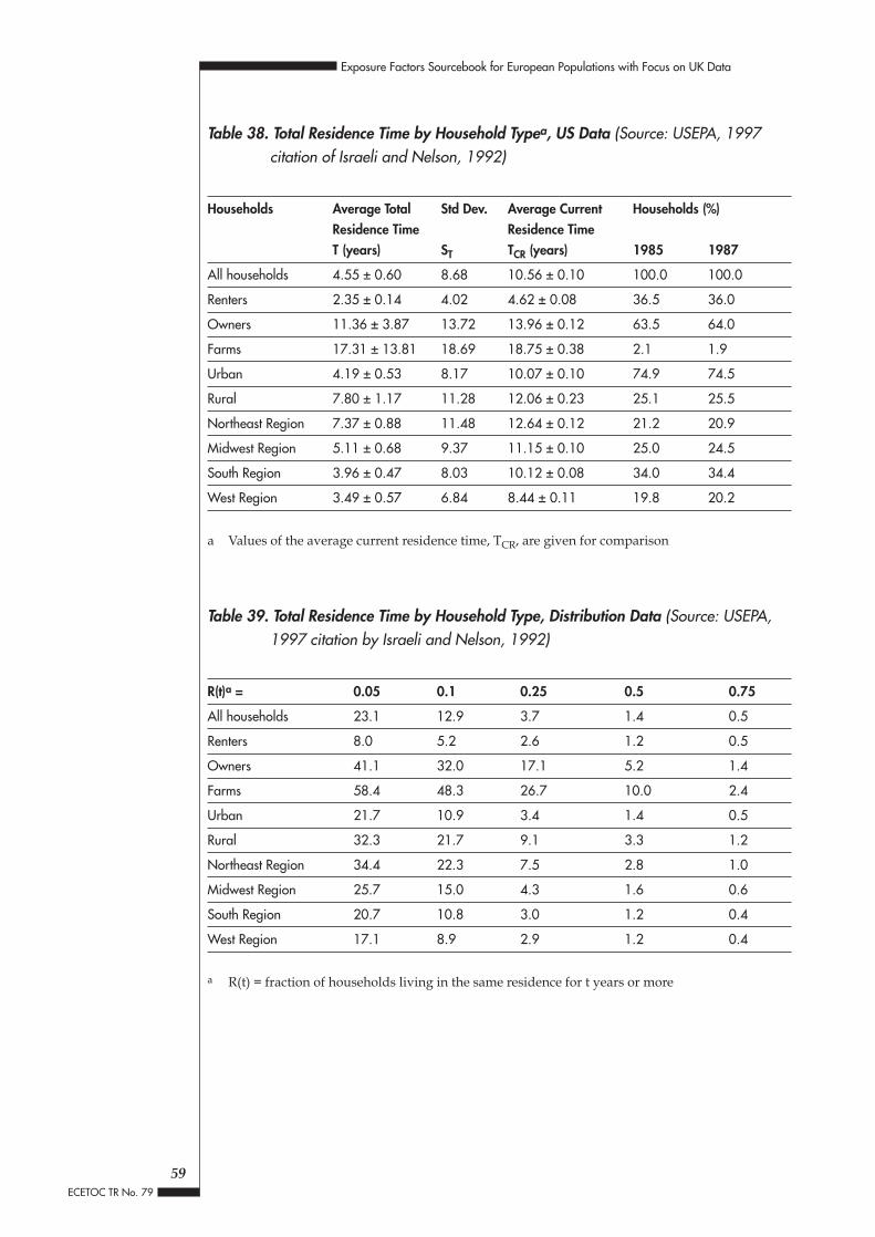
Table 38. Total Residence Time by Household Typea, US Data (Source: USEPA, 1997citation of Israeli and Nelson, 1992)

Households Average Total Std Dev. Average Current Households (%)Residence Time Residence TimeT (years) ST TCR (years) 1985 1987

All households 4.55 ± 0.60 8.68 10.56 ± 0.10 100.0 100.0

Renters 2.35 ± 0.14 4.02 4.62 ± 0.08 36.5 36.0

Owners 11.36 ± 3.87 13.72 13.96 ± 0.12 63.5 64.0

Farms 17.31 ± 13.81 18.69 18.75 ± 0.38 2.1 1.9

Urban 4.19 ± 0.53 8.17 10.07 ± 0.10 74.9 74.5

Rural 7.80 ± 1.17 11.28 12.06 ± 0.23 25.1 25.5

Northeast Region 7.37 ± 0.88 11.48 12.64 ± 0.12 21.2 20.9

Midwest Region 5.11 ± 0.68 9.37 11.15 ± 0.10 25.0 24.5

South Region 3.96 ± 0.47 8.03 10.12 ± 0.08 34.0 34.4

West Region 3.49 ± 0.57 6.84 8.44 ± 0.11 19.8 20.2

a Values of the average current residence time, TCR, are given for comparison

Table 39. Total Residence Time by Household Type, Distribution Data (Source: USEPA,1997 citation by Israeli and Nelson, 1992)

R(t)a = 0.05 0.1 0.25 0.5 0.75

All households 23.1 12.9 3.7 1.4 0.5

Renters 8.0 5.2 2.6 1.2 0.5

Owners 41.1 32.0 17.1 5.2 1.4

Farms 58.4 48.3 26.7 10.0 2.4

Urban 21.7 10.9 3.4 1.4 0.5

Rural 32.3 21.7 9.1 3.3 1.2

Northeast Region 34.4 22.3 7.5 2.8 1.0

Midwest Region 25.7 15.0 4.3 1.6 0.6

South Region 20.7 10.8 3.0 1.2 0.4

West Region 17.1 8.9 2.9 1.2 0.4

a R(t) = fraction of households living in the same residence for t years or more

59


ECETOC TR No. 79

4.11 School Tenure

SummaryData provided by the UK Department for Education and Employment indicate thattypical UK school tenures are 7 years for primary school and 5 years at secondary school.UK data for typical tenure in pre-school or additional voluntary education were notidentified.

Relevant StudiesInformation on typical patterns of school attendance was provided by the UK Departmentfor Education and Employment. School is compulsory for children between the ages of5-16: primary school for ages 5-11 and secondary school for ages 12-16 (DFEE, 2000a).In England and Wales, compulsory school age commences from the first term after achild's fifth birthday until the last Friday in June in the school year in which the childturns sixteen (DFEE, 2000b).

60


ECETOC TR No. 79

5. RECEPTOR CONTACT RATES

5.1 Soil Ingestion Rates

SummaryMedian soil ingestion rates are estimated as 40 mg/day and 1 mg/day for children andadults, respectively, based upon the studies of Calabrese et al (1997) and Stanek et al(1997). These data are based upon US studies, but represent the best available information.Data on soil ingestion rates are limited and variable. Region specific differences in childplay and hygienic patterns will likely affect typical soil consumption. The currentdata set are too limited, however, to predict what level of regional variation might beexpected, and to prepare distributions of soil ingestion rates. Available data supportupper limits of 200 mg/day for children and 300 mg/day for adults. Adult soil ingestionis generally expected to be lower than that of children, based upon age related behaviouralpatterns. The higher upper limit for adults is related to data variability and indicatesthe uncertainty in current estimates. The recommended values are based upon studiesperformed in the summer or autumn; soil ingestion during winter is likely lower.

Relevant StudiesInadvertent soil and dust consumption can occur via food adherence or mouthing ofobjects or hands. Soil ingestion is probably greater for children than adults due to childbehavioural patterns, for example crawling, playing in dirt, and mouthing. Deliberatesoil ingestion, or soil pica, is an uncommon behavioural pattern. Very limited dataare available on the soil ingestion rates for such individuals. Since soil pica is notconsidered a typical behaviour, soil ingestion rates for population-based risk assessmentsare better estimated from studies in subgroups not exhibiting this behaviour. The recentreview of Simon (1998) can be consulted for further information on deliberate soilingestion.

In the first attempt to estimate soil ingestion quantitatively, Binder et al (1986) measuredlevels of soil tracer elements Al, Si, and Ti in feces. These elements were selected sincetheir concentration is high in soil but low in food and their gastrointestinal absorptionis low. The amount of soil ingested was calculated based on the fecal and soilconcentrations of the tracer elements and the amount of fecal output. Using similarmethodology, Clausing et al (1987) and van Wijnen et al (1990) estimated the amountof soil consumed by children living in the Netherlands. The authors of all of these studieswere unable to resolve the widely differing estimates based on the various tracers. Thesedifferences were due primarily to lack of accounting for the presence of tracers in food,medicines, diapers and other materials that contact the faeces. For these reasons, thesoil ingestion estimates from these studies are considered unreliable.

Calabrese et al (1989) and Davis et al (1990) used a mass balance approach to estimatesoil ingestion in children. With this approach, the levels of tracer substances are measuredin food as well as soil and feces of study participants and non-food and soil sources oftracers are minimized. The amount of soil ingested is the difference of the total amount

61


ECETOC TR No. 79

of tracer substance in faeces minus the contribution from food. These studies provide amore accurate estimate of soil ingestion. However, the major sources of errors stillremaining in these studies are due to: 1) transit time error, which is reflected ininput/output misalignment due to both study design limitations and the presence ofhigh background levels of tracers in ingested food relative to ingested soil; and 2)unknown source error, i.e., non-food non-soil sources for certain elements, particularlyTi. Nonetheless, these studies provided better estimates of soil ingestion.

Based on the knowledge gained from identifying sources of errors in soil ingestionstudies, a detection limit model and guidance for selecting tracers for soil ingestionstudies were developed (Stanek and Calabrese, 1991; Calabrese and Stanek, 1991;Calabrese and Stanek, 1993; Stanek and Calabrese, 1994). This model relates the logmean square error in percent recovery to the log of the food/soil ratio. The detectionlimit model and guidance evolved into the “Best Tracer Method” (BTM) which involvesordering of trace elements for each subject-week, based on the food to soil tracer ingestionratio during the week (Stanek and Calabrese, 1995; Calabrese and Stanek, 1995).

The BTM was applied retrospectively to analyse the data from the Calabrese et al (1989)and Davis et al (1990) studies. The collective data suggest that the median soil ingestionrate for children is 30-40 mg/day, while the upper 95% estimate is approximately 200mg/day (Stanek and Calabrese, 1995).

A 7-day mass-balance study of 65 representative children ages 1-4 from Anaconda,Montana, using eight soil tracer substances has recently been conducted (Calabreseet al, 1997). The study design included a longer mass-balance period, as well as detailedtracer suppression for food items high in tracer elements included in the study bothbefore and during the sample collection period, and a stronger adult validation study.Using the BTM method, the five best tracer elements were identified as Al, Si, TI, Y, andZr. According to the BTM, the median soil ingestion was less than 1 mg/day whilethe upper 95% was 160 mg/day. Based on improvements in study design and analysis,these data may arguably provide the most reliable estimates of soil ingestion in childrencurrently available. However, the study area was a grassy Superfund site. It is possiblethat the physical nature of the site and possible changes in activity patterns associatedwith Superfund designation could have led to a depression in soil ingestion rates in thisstudy.

Two soil ingestion studies in adults have been conducted using a mass balance approach,as part of larger studies in children (Calabrese et al, 1990, Stanek et al, 1997). In the morerecent study, ten adults received daily soil capsules containing 20, 100, and 500-mg soil,respectively. A 1-week period separated each study week. Based on 3 weeks ofobservation, after subtracting the capsule ingestion amounts, the study resulted in amedian estimate of 1 mg/day based upon the median of the three trace elements Al, Si,and Y. The 95th percentile was 330 mg/day and the average estimate of soil ingestionwas 10 mg/day. These findings represent lower levels of soil ingestion in adults thanin the previous mass balance pilot study. However, given the improved study design,the data from the more recent mass balance study by Stanek et al (1997), described above,should be considered as the best estimate of a soil ingestion rate in adults.

One limitation of all tracer studies is that they cannot distinguish between the contributionof indoor (dust) vs. outdoor (soil) to tracer element excretory output. Concentrations of

62


ECETOC TR No. 79

tracer elements are generally lower in dust than in soil (Stanek and Calabrese, 1993).Ingestion of household dust from non-soil sources can introduce a bias in the resultsof soil ingestion tracer studies. Calabrese and Stanek (1992) reported a statistical methodto account for the proportion of household dust derived from outdoor sources. Basedon this initial work, they estimated that approximately 30% of household dust is fromoutdoor soil and suggested revising soil ingestion estimates from tracer studiesdownwards by 31-35%.

In a later publication, this investigative team reported four different methods fordistinguishing soil versus dust ingestion: 1) duration correlation; 2) group tracer ratios;3) individual tracer ratios; and 4) combined multiple simultaneous estimates (Stanekand Calabrese, 1993). They noted that the reliability of the estimate is dependent on theapproach used as well as specific features of the individual soil ingestion study such asthe soil tracer used. Likely, personal hygiene and household factors also markedlyinfluence these estimates. For technical reasons, the authors placed more reliance onmethod 3, which indicated that about half of the residual fecal tracers are of dust origin.Given the uncertainties in the estimates, it is not possible at this time to quantify withcertainty the proportion of household dust derived from outdoor vs. indoor sourcesor the proportion of "soil ingestion" represented by soil vs. dust.

63


ECETOC TR No. 79

5.2 Soil Adherence to Skin

SummarySoil adherence to skin can vary depending upon soil properties, the type of activityresulting in soil contact, and the part of the body that is exposed. Most studies are of non-European populations, but these results are likely applicable to Europe: European datafor soil loading on hands falls within the range reported for non-European studies.Although EPA had previously specified an average and upper limit (USEPA, 1992b), itsrecommendations based upon more recent findings are to use soil adherence data thatare activity and body part specific (USEPA, 1997). Limited data on soil adherence byactivity and body part are provided in Table 40.

Relevant StudiesMost studies report soil adherence based upon soil loading to hands only. Mean valuesreported from these studies range from 0.5-1.5 mg/cm2 (USEPA, 1997). The results ofRoels et al (1980), a study of Belgian children, fall within this range (0.9- 1.5 mg/cm2,USEPA, 1997).

The recent work of Kissel et al (1996a, b as cited in USEPA, 1997) demonstrates that soilloading varies depending upon body part and activity (Table 40). Moisture content andparticle size can also affect soil adherence (USEPA, 1997).

The highest values for soil adherence are for the hands of children playing in mud (Table40 - geometric means of 35-58 mg/cm2). Soil adherence values for other activities in thesame study were 2 to 4 orders of magnitude lower. For the activities studied, geometricmeans for soil adherence (in mg/cm2) ranged from: 0.0063 - 50.0 for hands, 0.0019 -11.0 for arms, 0.0008-36.0 for legs, 0.0022 - 24.0 for feet, and 0.0026 - 0.10 for faces.

The EFH recommends that these recent results supercede previous recommendations forsoil adherence to skin (previous recommendations were an average of 0.2 mg/cm2, upperend of 1.0 mg/cm2 - USEPA, 1992b). It is recognised, however, that there is need foradditional data on soil adherence to skin.

64


ECETOC TR No. 79

Tabl

e 40

. Soi

l Adh

eren

ce b

y A

ctiv

ity a

nd B

ody

Regi

on (S

ourc

e: U

SEPA

, 199

7 ci

tatio

n of

Kiss

el e

t al,

1996

and

Hol

mes

et a

l, 19

96)

Act

ivity

Age

(yea

rs)

NDr

ess

Post

-Act

ivity

Der

mal

Soi

l Loa

ding

s (m

g/cm

2 )*

Geo

met

ric m

ean

(Geo

met

ric S

td D

ev.)

Han

dsA

rms

Legs

Feet

Face

s

INDO

OR

Tae

Kwon

Do

70.

0063

(1.9

)0.

0019

(4.1

)0.

002

(2.0

)0.

0022

(2.1

)G

reen

hous

e W

orke

rs2

0.04

30.

0064

0.00

150.

005

Indo

or k

ids

no. 1

6-13

43

of 4

in s

hort

pant

s, 2

of 4

in s

hort

sleev

es,

0.00

73 (1

.9)

0.00

42 (1

.9)

0.00

41 (2

.3)

0.01

2 (1

.4)

sock

s, n

o sh

oes

Indo

or k

ids

no. 2

3-13

65

of 6

long

pan

ts, 5

of 6

long

sle

eves

, soc

ks,

0.01

4 (1

.5)

0.00

41 (2

.0)

0.00

31 (1

.5)

0.00

91 (1

.7)

no s

hoes

Day

care

kid

s no

. 1a

1-6.

56

4 of

6 lo

ng p

ants,

4 o

f 6 s

hort

sleev

es, s

hoes

0.11

(1.9

)0.

026

(1.9

)0.

030

(1.7

)0.

079

(2.4

)D

ayca

re k

ids

no. 1

b1-

6.5

64

of 6

long

pan

ts, 4

of 6

sho

rt sle

eves

, no

shoe

s0.

15 (2

.1)

0.03

1 (1

.8)

0.02

3 (1

.2)

0.13

(0.0

44)

Day

care

kid

s no

. 21-

45

4 of

5 lo

ng p

ants,

3 o

f 5 lo

ng s

leev

es, a

ll0.

073

(1.6

)0.

023

(1.4

)0.

011

(1.4

)0.

044

(1.3

)ba

refo

ot fo

r par

t of t

he d

ayD

ayca

re k

ids

no. 3

1-4.

54

all l

ong

pant

s, 3

of 4

long

sle

eves

, soc

ks a

nd s

hoes

0.03

6 (1

.3)

0.01

2 (1

.2)

0.01

4 (3

.0)

0.00

53 (5

.1)

OU

TDO

OR

Socc

er n

o. 1

13-1

58

6 of

8 lo

ng s

leev

es, 4

of 8

long

pan

ts, 3

of 4

sho

rt0.

11 (1

.8)

0.01

1 (2

.0)

0.03

1 (3

.8)

0.01

2 (1

.5)

pant

s an

d sh

in g

uard

sSo

ccer

no.

28

0.03

5 (3

.9)

0.00

43 (2

.2)

0.01

4 (5

.3)

0.01

6 (1

.5)

Socc

er n

o. 3

70.

019

(1.5

)0.

0029

(2.2

)0.

0081

(1.6

)0.

012

(1.5

)G

roun

dske

eper

s no

. 12

0.01

50.

005

0.01

80.

0021

Gro

unds

keep

ers

no. 2

50.

098

(2.1

)0.

0021

(2.6

)0.

001

(1.5

)0.

010

(2.0

)G

roun

dske

eper

s no

. 37

0.03

(2.3

)0.

0022

(1.9

)0.

0009

(1.8

)0.

0040

0.00

44 (2

.6)

Gro

unds

keep

ers

no. 4

70.

045

(1.9

)0.

014

(1.8

)0.

0008

(1.9

)0.

018

0.00

26 (1

.6)

*G

eom

etric

Mea

n(G

eom

etric

Sta

ndar

d D

evia

tion)

65


ECETOC TR No. 79

Tabl

e 40

. Soi

l Adh

eren

ce b

y A

ctiv

ity a

nd B

ody

Regi

on (c

ontin

ued)

Act

ivity

Age

(yea

rs)

NDr

ess

Post

-Act

ivity

Der

mal

Soi

l Loa

ding

s (m

g/cm

2 )*

Geo

met

ric M

ean

(Geo

met

ric S

td D

ev.)

Han

dsA

rms

Legs

Feet

Face

s

OU

TDO

OR

Gro

unds

keep

ers

no. 5

80.

032

(1.7

)0.

022

(2.8

)0.

0010

(1.4

)0.

0039

(2.1

)La

ndsc

ape/

Rock

ery

40.

072

(2.1

)0.

030

(2.1

)0.

0057

(1.9

)Irr

igat

ion

Insta

llers

60.

19 (1

.6)

0.01

8 (3

.2)

0.00

54 (1

.8)

0.00

63 (1

.3)

Gar

dene

rs n

o. 1

80.

20 (1

.9)

0.05

0 (2

.1)

0.07

20.

017

0.05

8 (1

.6)

Gar

dene

rs n

o. 2

70.

18 (3

.4)

0.05

4 (2

.9)

0.02

2 (2

.0)

0.26

0.04

7 (1

.6)

Rugb

y no

. 18

0.40

(1.7

)0.

27 (1

.6)

0.36

(1.7

)0.

059

(2.7

)Ru

gby

no. 2

80.

14 (1

.4)

0.11

(1.6

)0.

15 (1

.6)

0.04

6 (1

.4)

Rugb

y no

. 37

0.04

9 (1

.7)

0.03

1 (1

.3)

0.05

7 (1

.2)

0.02

0 (1

.5)

Arc

haeo

logi

sts7

0.14

(1.3

)0.

041

(1.9

)0.

028

(4.1

)0.

24 (1

.4)

0.05

0 (1

.8)

Con

struc

tion

Wor

kers

80.

24 (1

.5)

0.09

8 (1

.5)

0.06

6 (1

.4)

0.02

9 (1

.6)

Util

ity W

orke

rs n

o. 1

50.

32 (1

.7)

0.20

(2.7

)0.

10 (1

.5)

Util

ity W

orke

rs n

o. 2

60.

27 (2

.1)

0.30

(1.8

)0.

10 (1

.5)

Equi

p. O

pera

tors

no.

14

0.26

(2.5

)0.

089

(1.6

)0.

10 (1

.4)

Equi

p. O

pera

tors

no.

24

0.32

(1.6

)0.

27 (1

.4)

0.23

(1.7

)Fa

rmer

s no

. 14

0.41

(1.6

)0.

059

(3.2

)0.

0058

(2.7

)0.

018

(1.4

)Fa

rmer

s no

. 26

0.47

(1.4

)0.

13 (2

.2)

0.03

7 (3

.9)

0.04

1 (3

.0)

Reed

Gat

here

rs4

0.66

(1.8

)0.

036

(2.1

)0.

16 (9

.2)

0.63

(7.1

)Ki

ds-in

-mud

no.

19-

146

all i

n sh

ort s

leev

e T-

shirt

s, s

horts

, bar

efoo

t35

(2.3

)11

(6.1

)36

(2.0

)24

(3.6

)Ki

ds-in

-mud

no.

29-

146

all i

n sh

ort s

leev

e T-

shirt

s, s

horts

, bar

efoo

t58

(2.3

)11

(3.8

)9.

5 (2

.3)

6.7

(12.

4)

*G

eom

etric

Mea

n(G

eom

etric

Sta

ndar

d D

evia

tion)

66


ECETOC TR No. 79

5.3 Inhalation Rates

SummaryShort-term (hourly) and long-term (daily) inhalation rates are presented in Tables 41and 42, respectively. These values are based upon US data, but are probably representativeof Europeans as well.

Relevant StudiesInhalation rate, also referred to as ventilation rate (VR), will vary depending uponage, gender, weight, health status and level of activity. Ventilation rates are typicallymeasured as minute volume (l of air exhaled/minute), calculated as the volume of airrespired in each breath (tidal volume) multiplied by the number of breaths/minute(USEPA, 1997).

Reported literature values for VR are based upon a number of methods (Layton, 1993).These include direct measurement of respired volume, indirectly from heart rate (HR)measurements or self-estimates. The direct method works well for controlled settings,but is not practical for normal living conditions as it requires that a person wear a devicefor monitoring airflow. For the indirect HR method, HR and VR are measured for a givenindividual under a variety of physical activities in a controlled setting. Thesemeasurements are used to develop equations relating VR to HR. Heart rate, which isless cumbersome to monitor than air flow, is then recorded during normal activities.Ventilation rates are then calculated based upon the VR-HR correlation equations.

Estimates of daily inhalation rate have been based upon the short-term data describedabove. Inhalation rates are typically grouped into several activity levels. For each activitylevel, the average inhalation rate is multiplied by the daily time spent at that level. Adaily inhalation rate is then calculated by summing the volume of air inhaled for eachactivity level over the course of a day.

Recently, it has been shown that daily inhalation rates based upon the calculationsdescribed above exceed inhalation rates that could be sustained based upon foodconsumption data (Layton, 1993). The above methods may be used for estimatinginhalation rates for short-term exposures, but do not appear to be appropriate for estimatesof long-term average inhalation (possibly due to differences in long-term vs. short-termactivity patterns). The USEPA recently evaluated available inhalation rate data (USEPA,1997), and developed the short-term and long-term recommendations summarised inTable 41 and 42. These recommendations are based primarily upon data for the USpopulation, but they can be applied to European populations as well.

5.3.1 Short-term rates (hourly inhalation rates by activity level)

The short-term data, separated by age, gender, and activity level, should be reasonablyrepresentative of people of any nationality. For a given activity, a similar inhalation ratewould be expected for a person of similar body size and gender. This is supported bythe similarity of the short-term data to reference inhalation rates reported by ICRP(Snyder et al, 1975, Table 41). Basal metabolism is related to body weight (Layton, 1993)

67

Exposure Factors Sourcebook for European Population with Focus on UK Data

ECETOC TR No. 79

and will be similar for UK and US populations given the similarity in body weight.Between ethnic groups, minuted ventilation rates are generally similar (Roy et al, 1991).

Inhalation rate data are considered inadequate for estimating distributions for inhalationrates (USEPA, 1997). McKone and Daniel (1991) developed equations relating inhalationrate to body weight for the ICRP data (Table 41). Since they were based upon ICRP data,these equations result in similar values for resting and light activity as ICRP. Using theseequations and body weight distributions, distributions can be developed for inhalationrates. This approach is suggested with caution, however: the McKone and Danielequations are based upon extremely limited data (N=2 for children, N=9 for adults).Any inhalation rate distributions developed should be cross-checked with the range ofinhalation rates reported in the literature for similar levels of activity.

Another possible source of inhalation rate distributions for children is the work ofRusconi et al (1994). This reference was not evaluated in USEPA (1997). It providesdistributions for breathing rate (breaths/minute) by age for Italian children aged 15days to 3 years old. Respiratory rates were measured for 618 healthy children whenawake and calm and when asleep. Repeatability of results was good. Mean, median,and standard deviation of respiratory rate in breaths/minute are provided in Table43. Centile curves were estimated for each age group as follows:

Awake Data: Log10(RR) = (1.6801 + 0.08592Zi) - (0.01189 + 0.0004301Zi)x + 0.0001340x2

Asleep Data: Log10(RR) = (1.5773 + 0.09196Zi) - (0.01314 + 0.0005155Zi)x + 0.0001765x2

Where Zi = is the normal equivalent deviate corresponding to an ith percentile (forexample, Z95 = 1.645) and x = age in months.

If tidal volume data (volume of air exhaled/breath) are available, the equations providedcan be used to develop inhalation rate distributions. Tidal volume, however, will varywith age and limited data are available for this age group. Tidal volume for children aresummarised for this age group in Table 44.

5.3.2 Long-term rates (average daily inhalation rates)

The long-term recommendations in Table 42 are based upon the development ofmetabolically consistent breathing rates by Layton (1993). Layton used three energy-based approaches for estimating daily inhalation rates: average daily intakes of foodenergy from dietary surveys, with an upward adjustment to account for under reportingof food consumption; average daily energy expenditure based upon the ratio of totaldaily expenditure to basal metabolism; and daily energy expenditures based upon time-activity data. The first two approaches yielded consistent results (9.7-11 m3/day and13-17 m3/day for adult females, and males, respectively). When compared to the firsttwo approaches, the third approach yielded estimates that were greater for females butsimilar for males (11-15 m3/day and 13-17 m3/day for females and males, respectively).Values from all approaches were below those of the ICRP reference values for males andfemales (21 and 23 m3/day, respectively; Snyder et al, 1975).

68


ECETOC TR No. 79

The long-term estimate based upon food consumption and long-term energy expendituremay show greater difference among populations given differences in lifestyles andactivity levels. However, the estimate of Layton, 1993 is still probably a reasonablerepresentative of European populations as well. Layton used adult food energy intakesof 1400-2400 kcal/day (depending upon age and gender), with caloric intake beingapproximately 40% fat, 16% protein and 44% carbohydrate. Results of the 1997 UKNational Food Survey yield comparable energy intake: an average of 1900 kcal/day,with 38% from fat, 15% protein, and 47% carbohydrate (Slater et al, 1998), and thus wouldresult in similar metabolic oxygen demand (11 m3/day average, includes males andfemales all ages). The 1992-1993 National Diet and Nutrition Survey of British childrenaged 1.5-4.5 years resulted in a mean energy intake of 1184 kcal/day for boys and1118 kcal/day for girls, with 36% from fat, 13% from protein and 52% from carbohydrate(Davies, 1997) and results in a daily inhalation rate of 6.5 m3/day. The analysis andresults of Layton, which were verified for consistency using more than one data set andapproach, are reasonable approximations of long-term daily inhalation rates for the UKpopulation and probably for European populations in general.

Table 41. Short-term Inhalation Rates (m3/hour) (Source: USEPA, 1997)

Population Activity Level Mean Comparison with other studiesICRP Reference Man McKone and Daniels, 1991*(Snyder et al, 1975)

AdultsRest 0.4 0.45 M, 0.36 F 0.396Sedentary 0.5Light 1.0 1.2 M, 1.14 F active: 1.2Moderate 1.6Heavy 3.2 2.6 M, 1.5 F

Maximal exercise: 6.7 M,5.4 F

ChildrenRest 0.3 0.288 0.297Sedentary 0.4Light 1.0 0.78 active: 0.81Moderate 1.2Heavy 1.9

Maximal exercise: 2.0 - 6.8Outdoor Workers

Slow 1.1Moderate 1.5Heavy 2.5Hourly Average 1.3**

* Based upon the following equations:child resting IR (m3/hr) = 0.011 x Body weight, average body weight of 27 kg usedchild active IR ( m3/hr) = 0.030 x Body weight, average body weight of 27 kg usedadult resting IR ( m3/hr) = 0.006 x Body weight, average body weight of 66 kg usedadult active IR ( m3/hr) = 0.018 x Body weight, average body weight of 66 kg used

** Upper percentile of 3.3

69


ECETOC TR No. 79

Table 42. Long-term Inhalation Rates (m3/day) (Source: USEPA, 1997)

Population Gender Mean Comparison with other studiesICRP Reference Man(Snyder et al, 1975)

Adults19 - 65 + yrs F 11.3 21

M 15.2 23

Children15 - 18 yrs F 12.0

M 17.012 - 14 yrs F 12.0

M 15.09 - 11 yrs F 13.0 M and F: 15

M 14.06 - 8 yrs 10.03 - 5yrs 8.31 - 2 yrs 6.8

Infants< 1 yr 4.5 3.8 - 4.7 for 1 yr old, 0.8 for newborn

Table 43. Respiratory Rate for Children up to 3 Years of Age (Source: Rusconi et al,1994)

Age (months) N Values in breaths/minuteSubjects Awake Subjects AsleepMean Median Std Dev. Mean Median Std Dev.

< 2 104 48.0 47 9.1 39.8 39 8.7

2 to < 6 106 44.1 42 9.9 33.4 32 7.0

6 to < 12 126 39.1 38 8.5 29.6 28 7.0

12 to < 18 77 34.5 34 5.8 27.2 26 5.6

18 to < 24 65 32.0 32 4.8 25.3 24 4.6

24 to < 30 79 30.0 30 6.2 23.1 23 4.6

30 to < 36 61 27.1 28 4.1 21.5 21 3.7

70


ECETOC TR No. 79

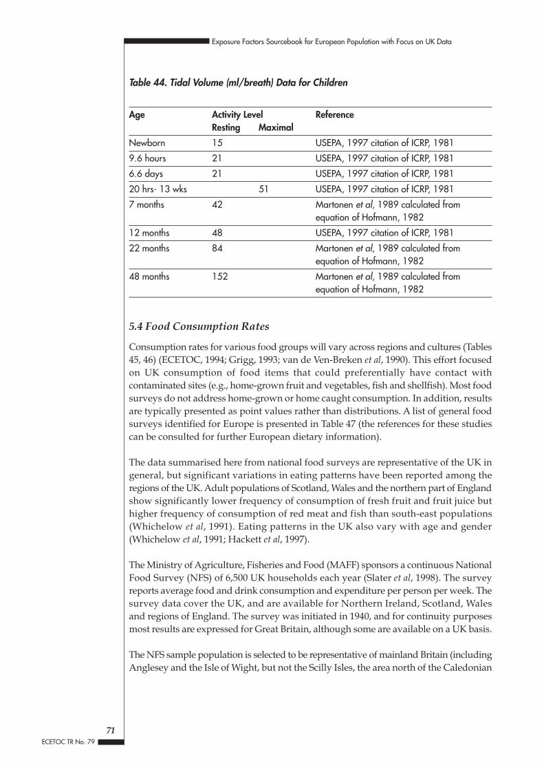
Table 44. Tidal Volume (ml/breath) Data for Children

Age Activity Level ReferenceResting Maximal

Newborn 15 USEPA, 1997 citation of ICRP, 1981

9.6 hours 21 USEPA, 1997 citation of ICRP, 1981

6.6 days 21 USEPA, 1997 citation of ICRP, 1981

20 hrs- 13 wks 51 USEPA, 1997 citation of ICRP, 1981

7 months 42 Martonen et al, 1989 calculated fromequation of Hofmann, 1982

12 months 48 USEPA, 1997 citation of ICRP, 1981

22 months 84 Martonen et al, 1989 calculated from equation of Hofmann, 1982

48 months 152 Martonen et al, 1989 calculated fromequation of Hofmann, 1982

5.4 Food Consumption Rates

Consumption rates for various food groups will vary across regions and cultures (Tables45, 46) (ECETOC, 1994; Grigg, 1993; van de Ven-Breken et al, 1990). This effort focusedon UK consumption of food items that could preferentially have contact withcontaminated sites (e.g., home-grown fruit and vegetables, fish and shellfish). Most foodsurveys do not address home-grown or home caught consumption. In addition, resultsare typically presented as point values rather than distributions. A list of general foodsurveys identified for Europe is presented in Table 47 (the references for these studiescan be consulted for further European dietary information).

The data summarised here from national food surveys are representative of the UK ingeneral, but significant variations in eating patterns have been reported among theregions of the UK. Adult populations of Scotland, Wales and the northern part of Englandshow significantly lower frequency of consumption of fresh fruit and fruit juice buthigher frequency of consumption of red meat and fish than south-east populations(Whichelow et al, 1991). Eating patterns in the UK also vary with age and gender(Whichelow et al, 1991; Hackett et al, 1997).

The Ministry of Agriculture, Fisheries and Food (MAFF) sponsors a continuous NationalFood Survey (NFS) of 6,500 UK households each year (Slater et al, 1998). The surveyreports average food and drink consumption and expenditure per person per week. Thesurvey data cover the UK, and are available for Northern Ireland, Scotland, Walesand regions of England. The survey was initiated in 1940, and for continuity purposesmost results are expressed for Great Britain, although some are available on a UK basis.

The NFS sample population is selected to be representative of mainland Britain (includingAnglesey and the Isle of Wight, but not the Scilly Isles, the area north of the Caledonian

71


ECETOC TR No. 79

Canal nor the islands off the Scottish mainland). Each household is surveyed for oneweek and the households surveyed are changed regularly. Surveys are performedcontinuously throughout the year.

Consumption estimates in the NFS are based upon food purchased, home-produced,and free food consumed (Slater et al, 1998). These data represent the quantity of foodentering the home, not individual consumption. Free food that is obtained from a personalfarm, garden, business, hedgerow or allotment is recorded as it is used. Thus, values forthese food sources may be more representative of actual consumption than values forpurchased items, but waste and the number of household members consuming eachitem are not documented. Consumption data on food purchased and eaten outside ofthe home is also collected but analyzed separately.

Estimates of total dietary intake are also available from the MAFF National Diet andNutrition Surveys (NDNS) (Gregory et al, 1990, 1995). These surveys focus on specificage groups and are cross sectional studies designed to be representative of the nationalBritish population (England, Scotland and Wales).

For the NDNS of British children aged 1.5-4.5 years, a record of weighed dietary intakewas obtained for four consecutive days for each participating child (1675 childrenparticipated). Each four-day period included 2 weekend days and 2-week days, withMondays and Tuesdays being equally represented as Thursdays and Fridays. Informationfrom the 2-week days was weighted to 5 days and the weighted information added tothe 2 weekend days to calculate average daily intake. The survey was performed overa 12-month period (July 1992 - June 1993) to account for possible seasonal variationsin dietary intake. Foods eaten in and out of the home were included.

The NDNS does not provide any information on consumption of home-grown items.Home-grown consumption data, while extremely limited, are provided in the NFS; thus,NFS data serve as the basis for the estimates of home-grown consumption. Data aretaken from the 1997 main survey of Great Britain; the survey population was 75% adultsand 25% children (Slater et al, 1998).

72


ECETOC TR No. 79

Tabl

e 45

. Ave

rage

Foo

d Co

nsum

ptio

n in

the

Euro

pean

Com

mun

ity a

nd it

s M

embe

r Co

untri

es (S

ourc

e: E

CET

OC

, 199

4 ci

tatio

n of

Eur

omon

itor 1

992,

Euro

pean

Mar

ketin

g D

ata

and

Stat

istic

s. U

sed

with

per

miss

ion.

)

Inta

ke o

fA

vera

ge fo

od c

onsu

mpt

ion

(kg

per

capi

ta p

er y

ear)

Rang

eEC

BDK

FD

GR

IRL

IN

LP

SPU

Km

inm

ax

Mea

t194

.010

5.0

108.

910

9.9

104.

976

.487

.387

.588

.868

.495

.077

.368

.410

9.9

Beef

and

vea

l22

.022

.318

.130

.723

.719

.019

.026

.819

.313

.611

.517

.011

.530

.7Po

rk40

.749

.169

.137

.663

.222

.234

.730

.847

.625

.947

.424

.822

.269

.1O

ther

21.7

19.3

13.3

25.2

12.6

29.5

26.7

20.9

18.5

21.9

27.4

25.0

12.6

29.5

Fish

10.1

10.2

41.8

7.5

7.4

7.2

12.6

10.1

9.8

24.7

20.3

3.5

3.5

41.8

Milk

+ y

ogur

t82

.467

.874

.265

.865

.866

.917

3.6

69.7

79.3

52.1

102.

612

2.3

52.1

173.

6

Butte

r4.

98.

66.

98.

68.

51.

05.

52.

43.

90.

90.

64.

20.

68.

6

Che

ese

14.5

12.6

12.8

22.4

17.4

22.1

5.4

17.6

15.0

5.2

5.5

8.0

5.2

22.4

Frui

t + v

eget

able

s20

5.6

173.

814

9.8

194.

019

6.4

248.

314

8.3

277.

524

2.5

165.

425

2.6

131.

613

1.6

277.

5

Cer

eals

116.

598

.793

.110

1.8

99.6

145.

214

4.7

160.

074

.512

5.4

97.7

119.

674

.516

0.0

Pota

toes

83.3

97.6

62.9

73.6

69.6

86.4

140.

238

.087

.011

1.5

107.

010

6.7

38.0

140.

2

1To

tal d

oes

not r

efle

ct th

e su

m o

f the

sub

grou

ps

73


ECETOC TR No. 79

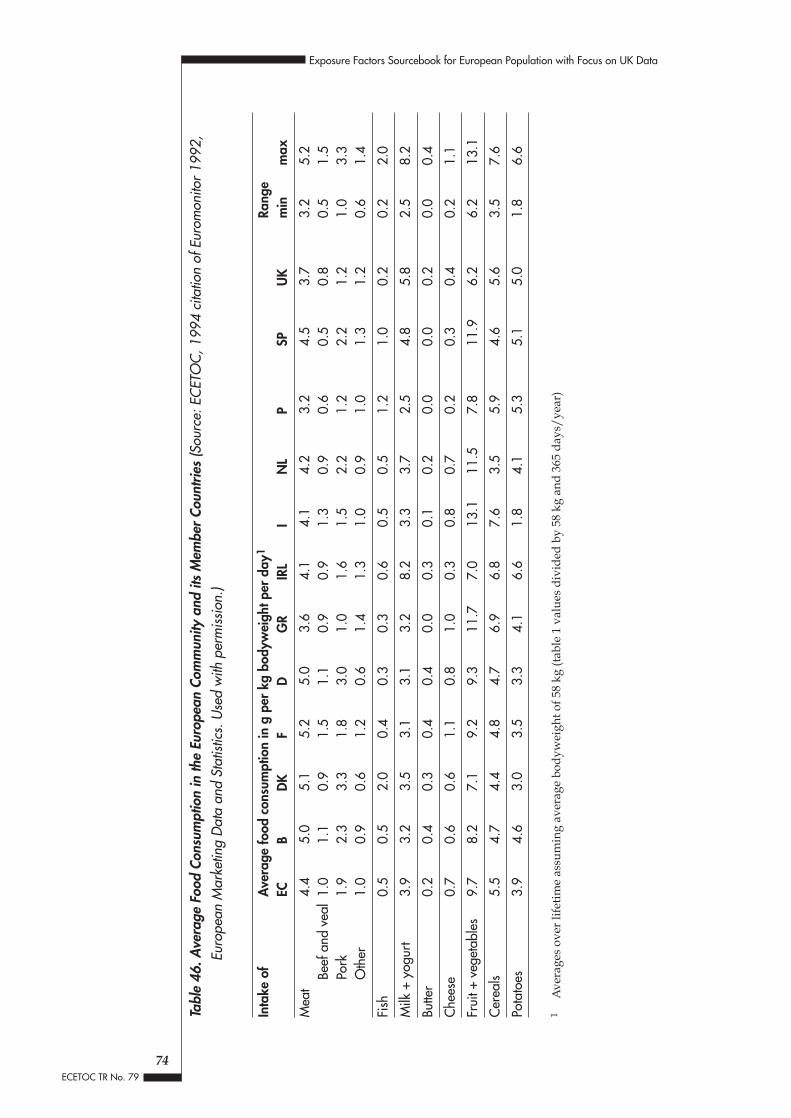
74


ECETOC TR No. 79

Tabl

e 46

. Ave

rage

Foo

d Co

nsum

ptio

n in

the

Euro

pean

Com

mun

ity a

nd it

s M

embe

r Co

untri

es (S

ourc

e: E

CET

OC

, 199

4 ci

tatio

n of

Eur

omon

itor 1

992,

Euro

pean

Mar

ketin

g D

ata

and

Stat

istic

s. U

sed

with

per

miss

ion.

)

Inta

ke o

fA

vera

ge fo

od c

onsu

mpt

ion

in g

per

kg

body

wei

ght p

er d

ay1

Rang

eEC

BDK

FD

GR

IRL

IN

LP

SPU

Km

inm

ax

Mea

t4.

45.

05.

15.

25.

03.

64.

14.

14.

23.

24.

53.

73.

25.

2Be

ef a

nd v

eal

1.0

1.1

0.9

1.5

1.1

0.9

0.9

1.3

0.9

0.6

0.5

0.8

0.5

1.5

Pork

1.9

2.3

3.3

1.8

3.0

1.0

1.6

1.5

2.2

1.2

2.2

1.2

1.0

3.3

Oth

er1.

00.

90.

61.

20.

61.

41.

31.

00.

91.

01.

31.

20.

61.

4

Fish

0.5

0.5

2.0

0.4

0.3

0.3

0.6

0.5

0.5

1.2

1.0

0.2

0.2

2.0

Milk

+ y

ogur

t3.

93.

23.

53.

13.

13.

28.

23.

33.

72.

54.

85.

82.

58.

2

Butte

r0.

20.

40.

30.

40.

40.

00.

30.

10.

20.

00.

00.

20.

00.

4

Che

ese

0.7

0.6

0.6

1.1

0.8

1.0

0.3

0.8

0.7

0.2

0.3

0.4

0.2

1.1

Frui

t + v

eget

able

s9.

78.

27.

19.

29.

311

.77.

013

.111

.57.

811

.96.

26.

213

.1

Cer

eals

5.5

4.7

4.4

4.8

4.7

6.9

6.8

7.6

3.5

5.9

4.6

5.6

3.5

7.6

Pota

toes

3.9

4.6

3.0

3.5

3.3

4.1

6.6

1.8

4.1

5.3

5.1

5.0

1.8

6.6

1A

vera

ges

over

life

time

assu

min

g av

erag

e bo

dyw

eigh

t of 5

8 kg

(tab

le 1

val

ues

divi

ded

by 5

8 kg

and

365

day

s/ye

ar)

75


ECETOC TR No. 79

Tabl

e 47

. Sur

veys

of E

urop

ean

Food

Con

sum

ptio

n or

Pur

chas

ing

Coun

try

Refe

renc

eFo

od It

emCo

mm

ents

Mul

tiple

Cou

ntrie

s:Va

rious

Eur

opea

n co

untri

esva

n de

Ven

-Bre

ken

et a

l, 19

90, s

tudy

by

revi

ew o

f die

tary

info

rmat

ion,

pro

vide

s re

fere

nces

for a

num

ber o

f stu

dies

, inc

lude

sD

utch

Insti

tute

for H

ealth

and

Env

ironm

ent

info

rmat

ion

on h

ome-

grow

n co

nsum

ptio

n-R

IVM

14 E

urop

ean

coun

tries

:TR

AN

SFA

IR s

tudy

, van

Pop

pel,

1998

studi

ed m

arke

t bas

kets

in 1

4 Eu

rope

an c

ount

ries,

then

100

food

sam

ples

repr

esen

tativ

eB,

DK,

FIN

, FR,

G, G

R, IC

L,of

the

tota

l fat

and

tran

s fa

tty a

cid

inta

ke w

ere

purc

hase

d in

199

5-19

96, a

naly

zed,

and

I, N

L, N

, P, S

, SW

, UK

TFA

inta

ke e

stim

ated

bas

ed u

pon

each

cou

ntry

's fo

od-c

onsu

mpt

ion

surv

ey d

ata

Euro

peG

rigg,

199

3A

llco

nsum

ptio

n an

d ea

ting

beha

viou

r diff

er b

y co

untry

Indi

vidu

al C

ount

ries

Den

mar

kA

nder

sen

et a

l, 19

96A

ll7

day

reco

rd, N

= 3

098,

per

form

ed in

199

5Fr

ance

SEC

OD

IP ,

Cha

mbo

lle e

t al,

1995

All

hous

ehol

d pu

rcha

ses

thro

ugho

ut a

yea

r, N

=600

0Fr

ance

Le F

ranc

ois

et a

l, 19

96A

llfo

od e

aten

out

side

of th

e ho

me

(Out

of H

ome

Food

Sur

vey

man

aged

by

CRE

DO

C, d

one

in 1

994)

Ger

man

y, D

ortm

und

area

DO

NA

LD s

tudy

, For

schu

ngsin

stitu

t für

infa

nts

and

youn

g pe

rson

s in

fam

ilies

from

favo

urab

le s

ocia

l bac

kgro

unds

, all,

3 d

ayKi

nder

nahr

ung,

Dor

tmun

d, c

ited

onw

eigh

ed d

iet r

ecor

dsEu

rope

an C

omm

issio

n w

eb p

age

Ger

man

ySc

hnei

der e

t al,

1995

Vege

tabl

esD

istrib

utio

nsG

reat

Brit

ain

Gre

gory

et a

l, 19

90A

llBr

itish

adu

lts d

iet s

tudy

Gre

at B

ritai

nM

ills

and

Tyle

r, 19

92A

llBr

itish

infa

nts

6-12

mon

ths

Gre

at B

ritai

nG

rego

ry e

t al,

1995

All

Briti

sh 1

.5-4

.5 y

rs o

ldN

ethe

rland

sD

utch

Nat

iona

l Foo

d C

onsu

mpt

ion

Surv

ey,

> 60

00 p

eopl

e, 1

0 di

ffere

nt a

ge g

roup

s an

d va

rious

food

cla

sses

, det

aile

d di

etar

y da

ta,

Hul

shof

and

Van

Sta

vere

n, 1

991

may

incl

ude

hom

e-gr

own

Russ

iaM

artin

chik

et a

l, 19

96A

llM

osco

w s

choo

lchi

ldre

n 10

and

15

yrs

old,

24

hr re

call

for 2

con

secu

tive

days

Scot

land

Payn

e an

d Be

lton,

199

2 A

ll7-

day

wei

ghte

d in

vent

ory

of fo

od a

nd n

utrie

nt in

take

for 1

53 h

ealth

y ch

ildre

n 2-

5 yr

s ol

din

Edi

nbur

ghSp

ain

Pére

z-Lla

ma

et a

l, 19

96A

llad

oles

cent

s in

SE

Spai

n, re

call

of p

revi

ous

24 h

r, re

lativ

e co

nsum

ptio

n of

var

ious

food

grou

psSp

ain

Estív

ariz

et a

l, 19

96M

ilk p

rodu

cts

Mad

rid s

choo

lchi

ldre

n, 2

4 hr

reca

ll fo

r 2 d

ays

and

estim

ated

food

inta

ke re

cord

for

2 da

ys

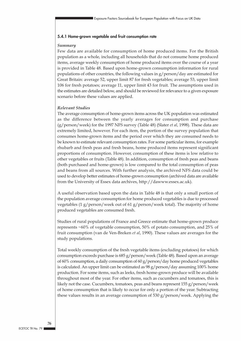
5.4.1 Home-grown vegetable and fruit consumption rate

SummaryFew data are available for consumption of home produced items. For the Britishpopulation as a whole, including all households that do not consume home produceditems, average weekly consumption of home produced items over the course of a yearis provided in Table 48. Based upon home-grown consumption information for ruralpopulations of other countries, the following values in g/person/day are estimated forGreat Britain: average 52, upper limit 87 for fresh vegetables; average 53, upper limit106 for fresh potatoes; average 11, upper limit 43 for fruit. The assumptions used inthe estimates are detailed below, and should be reviewed for relevance to a given exposurescenario before these values are applied.

Relevant StudiesThe average consumption of home-grown items across the UK population was estimatedas the difference between the yearly averages for consumption and purchase(g/person/week) for the 1997 NFS survey (Table 48) (Slater et al, 1998). These data areextremely limited, however. For each item, the portion of the survey population thatconsumes home-grown items and the period over which they are consumed needs tobe known to estimate relevant consumption rates. For some particular items, for examplerhubarb and fresh peas and fresh beans, home produced items represent significantproportions of consumption. However, consumption of these items is low relative toother vegetables or fruits (Table 48). In addition, consumption of fresh peas and beans(both purchased and home-grown) is low compared to the total consumption of peasand beans from all sources. With further analysis, the archived NFS data could beused to develop better estimates of home-grown consumption (archived data are availablefrom the University of Essex data archives, http://dawww.essex.ac.uk).

A useful observation based upon the data in Table 48 is that only a small portion ofthe population average consumption for home produced vegetables is due to processedvegetables (1 g/person/week out of 61 g/person/week total). The majority of homeproduced vegetables are consumed fresh.

Studies of rural populations of France and Greece estimate that home-grown producerepresents ~60% of vegetable consumption, 50% of potato consumption, and 25% offruit consumption (van de Ven-Breken et al, 1990). These values are averages for thestudy populations.

Total weekly consumption of the fresh vegetable items (excluding potatoes) for whichconsumption exceeds purchase is 685 g/person/week (Table 48). Based upon an averageof 60% consumption, a daily consumption of 60 g/person/day home produced vegetablesis calculated. An upper limit can be estimated as 98 g/person/day assuming 100% homeproduction. For some items, such as leeks, fresh home-grown produce will be availablethroughout most of the year. For other items, such as cucumbers and tomatoes, this islikely not the case. Cucumbers, tomatoes, peas and beans represent 155 g/person/weekof home consumption that is likely to occur for only a portion of the year. Subtractingthese values results in an average consumption of 530 g/person/week. Applying the

76


ECETOC TR No. 79

60% and 100% fractions as average and upper estimates to this value results in 45g/person/day as an average and 76 g/person/day as an upper estimate for consumptionof nonseasonal vegetables.

In the absence of specific data, an average yearly value for home-grown consumptionwas estimated assuming that each of the conditions above (all fresh vegetables availableor limited availability) apply for half a year. This results in a final average of 52g/person/day and upper limit of 87 g/person/day.

For potatoes, assuming home production accounts for 50% of fresh potato consumption,53 g/person/day is estimated as an average value. An upper limit of 106 g/person/dayis also calculated. Since potatoes store very well, consumption may occur throughoutthe entire year.

Total weekly fruit intake for categories where consumption exceeded purchase is 299g/person/week (Table 48). Assuming 25% of this is home-grown results in an averagedaily consumption of 11 g/person/day, with an upper limit of 43 g/person/day basedupon 100% home production. Since the predominant portion of this consumption isrelated to items which store well (apples, pears, frozen fruit), these values can be appliedover the course of a year.

Mean consumption of home-grown produce for a German population are presentedin Table 49 by age (Ihme, 1994). Consumption values for fruit and vegetables are greaterthan those estimated for the UK, while values for potatoes are lower. The countrydata in Table 45 indicate that per capita fruit and vegetable consumption in Germanyis 150% of the UK value, and German potato consumption is 65% that of the UK. Theestimated values for British vegetable and potato home-grown consumption are thusconsistent with the German values, but the British estimate of home-grown fruitconsumption is low in comparison. The relative ratios between adult and childconsumption may be applicable for countries in which similar age-specific dietarypatterns are expected. Detailed distributional information for US home-grownconsumption, by age, season and geographic region, is presented in the EFH (USEPA,1997).

77


ECETOC TR No. 79

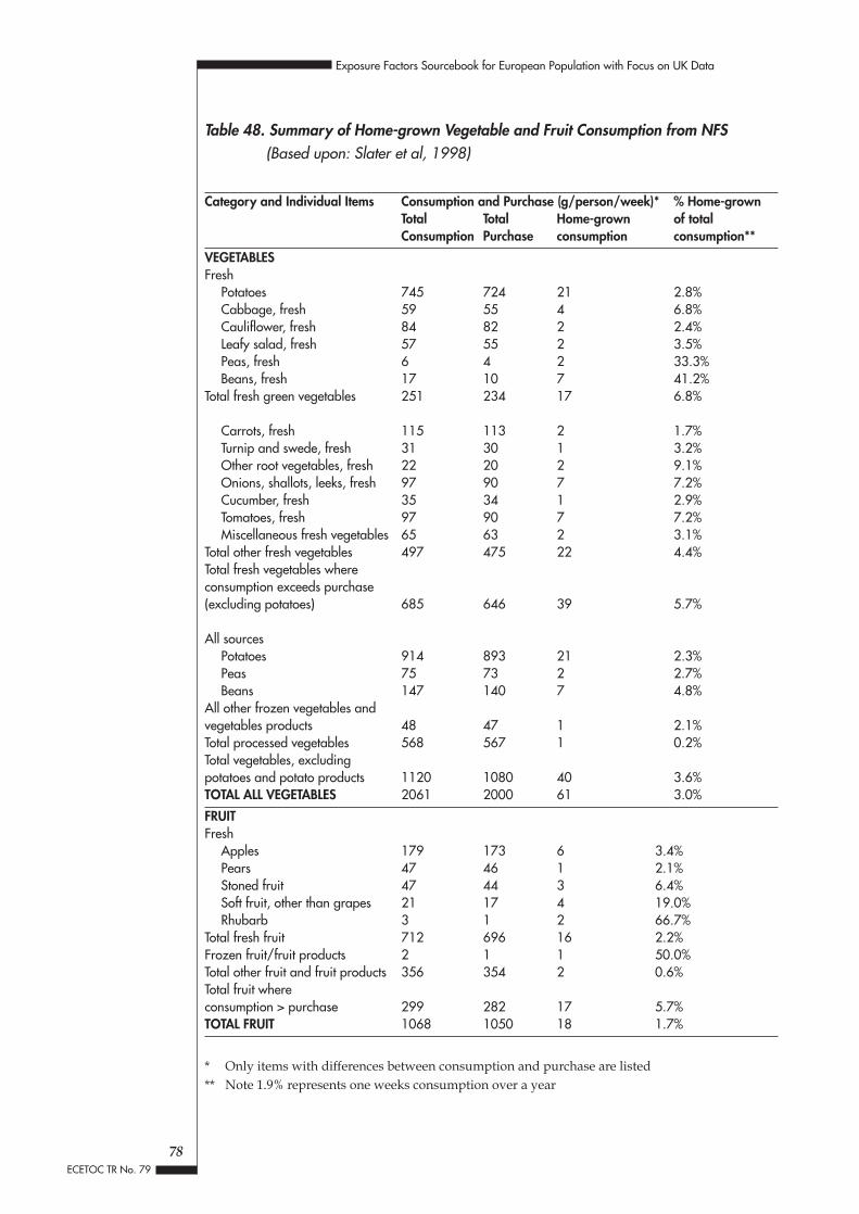
Table 48. Summary of Home-grown Vegetable and Fruit Consumption from NFS(Based upon: Slater et al, 1998)

Category and Individual Items Consumption and Purchase (g/person/week)* % Home-grownTotal Total Home-grown of totalConsumption Purchase consumption consumption**

VEGETABLESFresh

Potatoes 745 724 21 2.8%Cabbage, fresh 59 55 4 6.8%Cauliflower, fresh 84 82 2 2.4%Leafy salad, fresh 57 55 2 3.5%Peas, fresh 6 4 2 33.3%Beans, fresh 17 10 7 41.2%

Total fresh green vegetables 251 234 17 6.8%

Carrots, fresh 115 113 2 1.7%Turnip and swede, fresh 31 30 1 3.2%Other root vegetables, fresh 22 20 2 9.1%Onions, shallots, leeks, fresh 97 90 7 7.2%Cucumber, fresh 35 34 1 2.9%Tomatoes, fresh 97 90 7 7.2%Miscellaneous fresh vegetables 65 63 2 3.1%

Total other fresh vegetables 497 475 22 4.4%Total fresh vegetables whereconsumption exceeds purchase(excluding potatoes) 685 646 39 5.7%

All sourcesPotatoes 914 893 21 2.3%Peas 75 73 2 2.7%Beans 147 140 7 4.8%

All other frozen vegetables andvegetables products 48 47 1 2.1%Total processed vegetables 568 567 1 0.2%Total vegetables, excludingpotatoes and potato products 1120 1080 40 3.6%TOTAL ALL VEGETABLES 2061 2000 61 3.0%

FRUITFresh

Apples 179 173 6 3.4%Pears 47 46 1 2.1%Stoned fruit 47 44 3 6.4%Soft fruit, other than grapes 21 17 4 19.0%Rhubarb 3 1 2 66.7%

Total fresh fruit 712 696 16 2.2%Frozen fruit/fruit products 2 1 1 50.0%Total other fruit and fruit products 356 354 2 0.6%Total fruit whereconsumption > purchase 299 282 17 5.7%TOTAL FRUIT 1068 1050 18 1.7%

* Only items with differences between consumption and purchase are listed** Note 1.9% represents one weeks consumption over a year

78


ECETOC TR No. 79

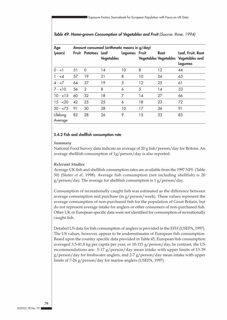
Table 49. Home-grown Consumption of Vegetables and Fruit (Source: Ihme, 1994)

Age Amount consumed (arithmetic means in g/day)(years) Fruit Potatoes Leaf Legumes Fruit Root Leaf, Fruit, Root

Vegetables Vegetables Vegetables Vegetables andLegumes

0 - <1 51 0 14 10 8 12 44

1 - <4 57 19 21 8 10 24 63

4 - <7 64 37 19 5 12 25 61

7 - <10 56 2 8 6 5 14 33

10 - <15 60 32 18 7 14 27 66

15 - <20 42 25 25 6 18 23 72

20 - <75 91 30 28 10 17 36 91

Lifelong 82 28 26 9 15 33 83Average

5.4.2 Fish and shellfish consumption rate

SummaryNational Food Survey data indicate an average of 20 g fish/person/day for Britons. Anaverage shellfish consumption of 1g/person/day is also reported.

Relevant StudiesAverage UK fish and shellfish consumption rates are available from the 1997 NFS (Table50) (Slater et al, 1998). Average fish consumption (not including shellfish) is 20g/person/day. The average for shellfish consumption is 1 g/person/day.

Consumption of recreationally caught fish was estimated as the difference betweenaverage consumption and purchase (in g/person/week). These values represent theaverage consumption of non-purchased fish for the population of Great Britain, butdo not represent average intake for anglers or other consumers of non-purchased fish.Other UK or European specific data were not identified for consumption of recreationallycaught fish.

Detailed US data for fish consumption of anglers is provided in the EFH (USEPA, 1997).The US values, however, appear to be underestimates of European fish consumption.Based upon the country specific data provided in Table 45, European fish consumptionaveraged 3.5-41.8 kg per capita per year, or 10-115 g/person/day. In contrast, the USrecommendations are: 5-17 g/person/day mean intake with upper limits of 13-39g/person/day for freshwater anglers, and 2-7 g/person/day mean intake with upperlimits of 7-26 g/person/day for marine anglers (USEPA, 1997).

79


ECETOC TR No. 79

Table 50. Summary of Fish Consumption from NFS (Source: Slater et al, 1998)

Values (g/person/week) % Non-purchasedConsumption Purchase Non-purchased

White, filleted, fresh 16 15 1 6.3%

White, unfilleted, fresh 2 2

White, uncooked, frozen 18 18

Fat, fresh, other than herring 13 12 1 7.7%

White, processed 6 5 1 16.7%

Fat, processed, filleted 2 2

Fat, processed, unfilleted 2 2

Shellfish 7 7

Cooked fish 11 11

Canned salmon 8 8

Other canned/bottled fish 23 23

Fish products, not frozen 11 11

Frozen convenience fish products 28 28

Total fish 146 144 2 1.4%

5.4.3 Meat and beef consumption rate

SummaryAverage beef consumption of 16 g/person/day and meat consumption of 134g/person/day is reported for the current UK population based upon the NFS datapresented in Table 51. For other European populations, the information provided inTables 45 and 46 can be used to estimate daily consumption.

Relevant StudiesAverage UK consumption data are available from the 1997 NFS (Slater et al, 1998).Distributions of consumption are not available. The data set for this study is archivedat the University of Essex. Data sets or analysis of the data can be requested on a feebasis.

The 1997 NFS estimates of beef and meat consumption (Table 51) are lower than theearlier UK data presented in Tables 45 and 46. Recent UK food surveys have noted adecline in beef consumption (Slater et al, 1998). It is unlikely that beef consumptionhas been reduced by the same level in other European countries. Thus, the data in Tables45 and 46 can be used as best estimates of beef and meat consumption for other countriesin Europe.

80


ECETOC TR No. 79

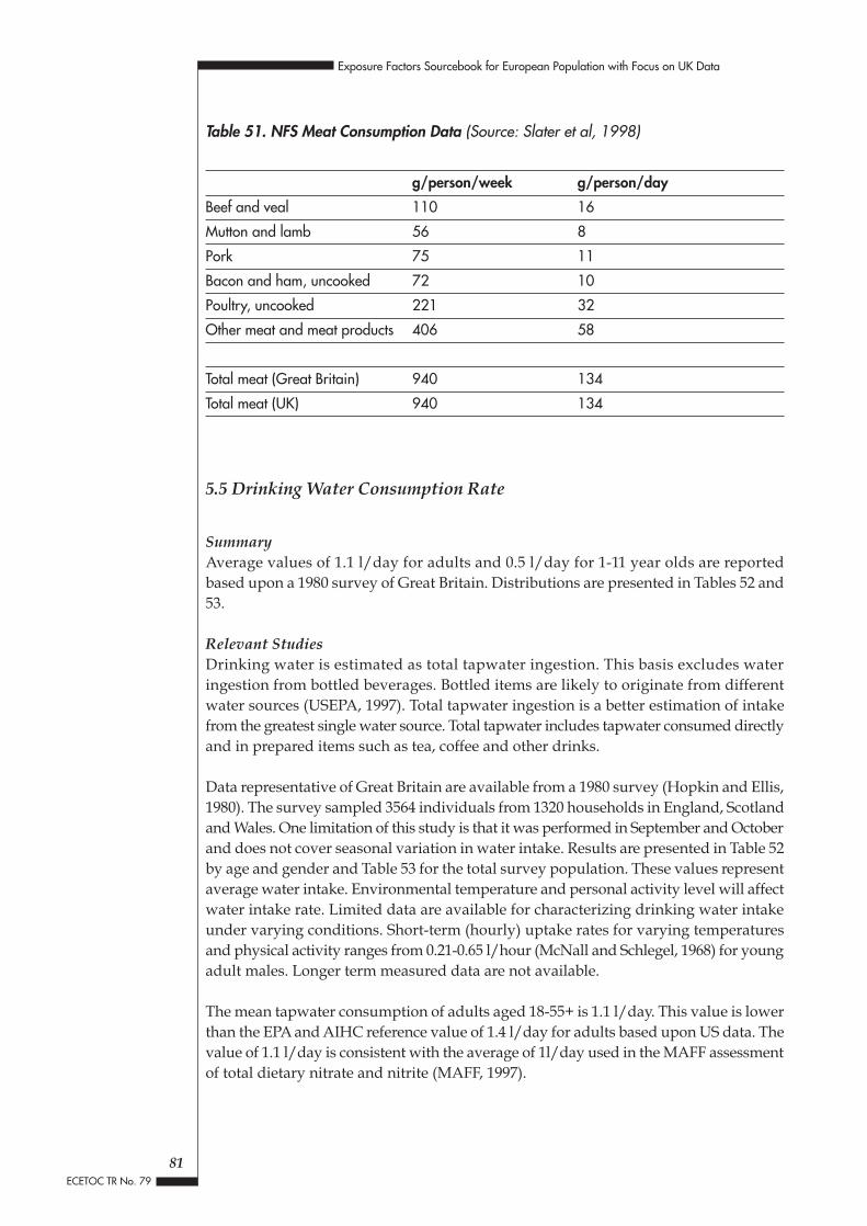
Table 51. NFS Meat Consumption Data (Source: Slater et al, 1998)

g/person/week g/person/day

Beef and veal 110 16

Mutton and lamb 56 8

Pork 75 11

Bacon and ham, uncooked 72 10

Poultry, uncooked 221 32

Other meat and meat products 406 58

Total meat (Great Britain) 940 134

Total meat (UK) 940 134

5.5 Drinking Water Consumption Rate

SummaryAverage values of 1.1 l/day for adults and 0.5 l/day for 1-11 year olds are reportedbased upon a 1980 survey of Great Britain. Distributions are presented in Tables 52 and53.

Relevant StudiesDrinking water is estimated as total tapwater ingestion. This basis excludes wateringestion from bottled beverages. Bottled items are likely to originate from differentwater sources (USEPA, 1997). Total tapwater ingestion is a better estimation of intakefrom the greatest single water source. Total tapwater includes tapwater consumed directlyand in prepared items such as tea, coffee and other drinks.

Data representative of Great Britain are available from a 1980 survey (Hopkin and Ellis,1980). The survey sampled 3564 individuals from 1320 households in England, Scotlandand Wales. One limitation of this study is that it was performed in September and Octoberand does not cover seasonal variation in water intake. Results are presented in Table 52by age and gender and Table 53 for the total survey population. These values representaverage water intake. Environmental temperature and personal activity level will affectwater intake rate. Limited data are available for characterizing drinking water intakeunder varying conditions. Short-term (hourly) uptake rates for varying temperaturesand physical activity ranges from 0.21-0.65 l/hour (McNall and Schlegel, 1968) for youngadult males. Longer term measured data are not available.

The mean tapwater consumption of adults aged 18-55+ is 1.1 l/day. This value is lowerthan the EPA and AIHC reference value of 1.4 l/day for adults based upon US data. Thevalue of 1.1 l/day is consistent with the average of 1l/day used in the MAFF assessmentof total dietary nitrate and nitrite (MAFF, 1997).

81


ECETOC TR No. 79

The survey of Hopkin and Ellis (1980) included tapwater intake for 1-4 and 5-11 yearolds. For 1-4 year olds the average daily intake was 0.47 l/day. This is lower than theaverage tapwater intake of 0.61-0.87 l/day based upon similarly aged Canadian children.However, it is greater than the intake of tapwater reported in a recent survey (1992-1993NDNS) of UK 1.5-4.5 year olds. The “tapwater” category from the NDNS survey includedwater used to prepare hot and cold drinks in addition to tapwater consumed directly.In addition, the NDNS data were collected over the course of a full year, so seasonalvariability is taken into account. The NDNS data also indicate that tapwater consumptionby the UK population may be lower than that of populations in Canada and the US.

Average tapwater intake, based upon the data of Hopkin and Ellis (1980) is 0.5 l/dayfor 1-11 year olds (Table 52).

82


ECETOC TR No. 79

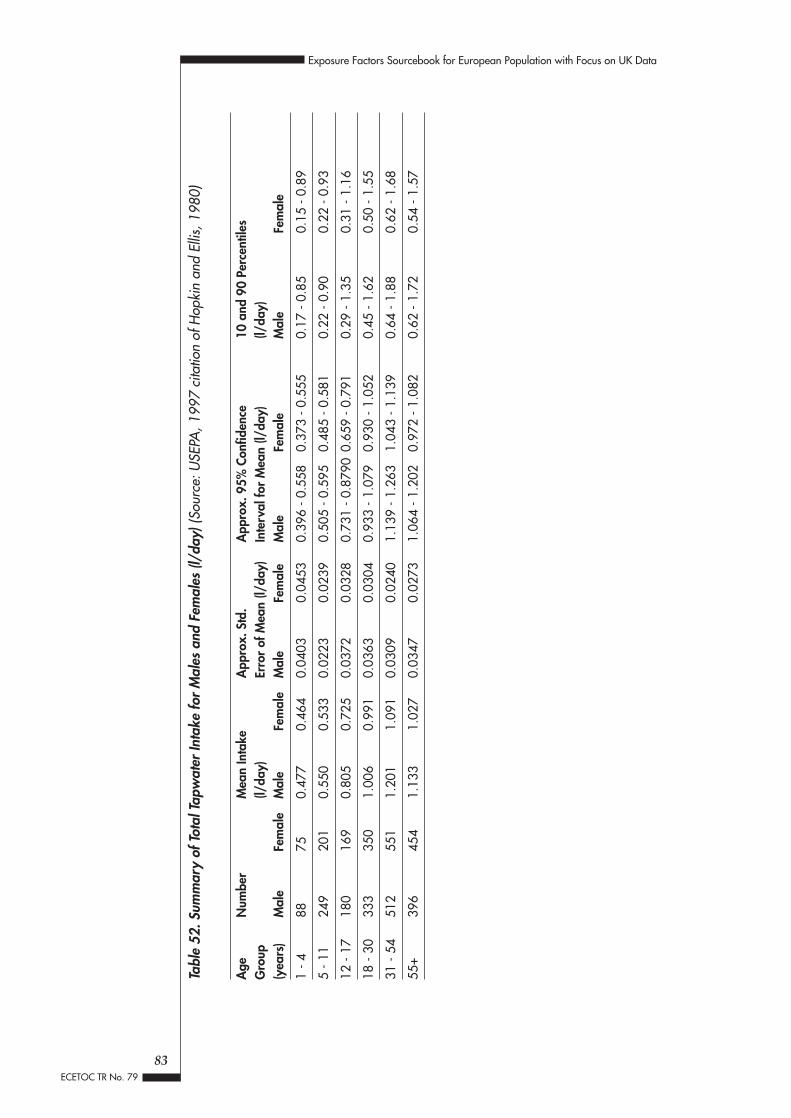
Tabl

e 52

. Sum

mar

y of

Tota

l Tap

wat

er In

take

for

Mal

es a

nd F

emal

es (l

/day

) (So

urce

: USE

PA, 1

997

cita

tion

of H

opki

n an

d El

lis, 1

980)

Age

Num

ber

Mea

n In

take

App

rox.

Std

.A

ppro

x. 9

5% C

onfid

ence

10 a

nd 9

0 Pe

rcen

tiles

Gro

up(l/

day)

Erro

r of

Mea

n (l/

day)

Inte

rval

for

Mea

n (l/

day)

(l/da

y)(y

ears

)M

ale

Fem

ale

Mal

eFe

mal

eM

ale

Fem

ale

Mal

eFe

mal

eM

ale

Fem

ale

1 - 4

8875

0.47

70.

464

0.04

030.

0453

0.39

6 - 0

.558

0.37

3 - 0

.555

0.17

- 0.

850.

15 -

0.89

5 - 1

124

920

10.

550

0.53

30.

0223

0.02

390.

505

- 0.5

950.

485

- 0.5

810.

22 -

0.90

0.22

- 0.

93

12 -

1718

016

90.

805

0.72

50.

0372

0.03

280.

731

- 0.8

790

0.65

9 - 0

.791

0.29

- 1.

350.

31 -

1.16

18 -

3033

335

01.

006

0.99

10.

0363

0.03

040.

933

- 1.0

790.

930

- 1.0

520.

45 -

1.62

0.50

- 1.

55

31 -

5451

255

11.

201

1.09

10.

0309

0.02

401.

139

- 1.2

631.

043

- 1.1

390.

64 -

1.88

0.62

- 1.

68

55+

396

454

1.13

31.

027

0.03

470.

0273

1.06

4 - 1

.202

0.97

2 - 1

.082

0.62

- 1.

720.

54 -

1.57

83


ECETOC TR No. 79

Tabl

e 53

. Int

ake

of To

tal L

iqui

d, To

tal T

apw

ater

, and

Var

ious

Bev

erag

es (l

/day

) (So

urce

: USE

PA, 1

997

cita

tion

of H

opki

n an

d El

lis, 1

980)

Beve

rage

All

Indi

vidu

als

Cons

umer

s O

nlya

Mea

nA

ppro

x.A

ppro

x. 9

5%10

and

90

1 an

d 99

Perc

enta

ge o

fM

ean

App

rox.

App

rox.

95%

Inta

keSt

d. E

rror

.Co

nfid

ence

Perc

entil

esPe

rcen

tiles

Tota

l Num

ber

Inta

keSt

d. E

rror

Conf

iden

ceof

Mea

nIn

terv

al fo

rof

Indi

vidu

als

of M

ean

Inte

rval

for

Mea

nM

ean

Tota

l Liq

uid

1.58

90.

0203

1.54

7 - 1

.629

0.77

- 2.

570.

34 -

4.50

100.

01.

589

0.02

031.

547

- 1.6

29

Tota

l Liq

uid

Hom

e1.

104

0.01

431.

075

- 1.1

330.

49 -

1.79

0.23

- 3.

1010

0.0

1.10

40.

0143

1.07

5 - 1

.133

Tota

l Liq

uid

Aw

ay0.

484

0.01

520.

454

- 0.5

140.

00 -

1.15

0.00

- 2.

8989

.90.

539

0.01

630.

506

- 0.5

72

Tota

l Tap

wat

er0.

955

0.01

290.

929

- 0.9

810.

39 -

1.57

0.10

- 2.

6099

.80.

958

0.01

290.

932

- 0.9

84

Tota

l Tap

wat

er H

ome

0.75

40.

0116

0.73

1 - 0

.777

0.26

- 1.

310.

02 -

2.30

99.4

0.75

90.

0116

0.73

6 - 0

.782

Tota

l Ta

pwat

er A

way

0.20

10.

0056

0.19

0 - 0

.212

0.00

- 0.

490.

00 -

0.96

79.6

0.25

30.

0063

0.24

0 - 0

.266

Tea

0.58

40.

0122

0.56

0 - 0

.608

0.01

- 1.

190.

00 -

2.03

90.9

0.64

30.

0125

0.61

8 - 0

.668

Cof

fee

0.19

00.

0059

0.17

8 - 0

.202

0.00

- 0.

560.

00 -

1.27

63.0

0.30

20.

0105

0.28

1 - 0

.323

Oth

er H

ot0.

011

0.00

150.

008

- 0.0

140.

00 -

0.00

0.00

- 0.

259.

20.

120

0.01

330.

093

- 0.1

47W

ater

Drin

ks

Col

d W

ater

0.10

30.

0049

0.09

3 - 0

.113

0.00

- 0.

310.

00-0

.85

51.0

0.20

30.

0083

0.18

6 - 0

.220

Frui

t Drin

ks0.

057

0.00

270.

052

- 0.0

620.

00 -

0.19

0.00

-0.4

946

.20.

123

0.00

490.

113

- 0.1

33

Non

Tap

wat

er0.

427

0.00

580.

415

- 0.4

390.

20 -

0.70

0.06

-1.2

799

.80.

428

0.00

580.

416

- 0.4

40

Hom

e-br

ew0.

010

0.00

170.

007

- 0.0

130.

00 -

0.00

0.00

-0.2

07.

00.

138

0.02

090.

096

- 0.1

80

Boug

ht A

lcoh

olic

0.20

60.

0123

0.18

1 - 0

.231

0.00

- 0.

680.

00-2

.33

43.5

0.47

40.

0250

0.42

4 - 0

.524

Beve

rage

s

aC

onsu

mer

s on

ly is

def

ined

as

only

thos

e in

divi

dual

s w

ho r

epor

ted

cons

umin

g th

e be

vera

ge d

urin

g th

e su

rvey

per

iod

84


ECETOC TR No. 79

5.6 Breast Milk Consumption Rate

SummaryIn the absence of more specific data, the USEPA recommendations summarised in Table58 can be used. The USEPA recommendations are based upon the weighted averages ofseveral studies and are similar to the values reported for Swedish infants (Table 57). For1-6 month old infants, mean daily breast milk intake is estimated as 742 ml with anupper percentile of 1033 ml. A 12-month average value of 688 ml/day with an upperpercentile of 980 ml/day can also be used. A cumulative distribution for the infantage at which British mothers stopped breast-feeding is presented in Table 55.

Relevant StudiesThe Ministry of Agriculture, Fisheries and Food (MAFF) sponsored a study of food andnutrient intakes of British infants (Mills and Tyler, 1992). The infant survey populationwas designed to be representative of children < 2 years old in Great Britain. The samplesize was 488 mothers and 491 infants (3 sets of twins). Overall, in the first 1-2 weeksafter birth, 55% of mothers solely breast-fed their child, 9% provided a combination ofbreast milk and infant formula, and 36% were solely bottle-fed. Incidence of breast-feeding varied by region (Table 54). A cumulative distribution for the number of weeksthat a mother breast-fed her child is presented in Table 55.

The amount of breast milk ingested was estimated only during the ages of 6-12 months.Breast milk consumption was not directly measured, but estimated based upon thenumber and duration of feedings. Feeding periods of ten minutes or longer were assumedto be full feeds. The ingested amount for a full feed was estimated as 135 g for infantsaged 6-7 months and 100 g for infants aged 8-12 months, based upon the data of Paulet al (1988). For feeding periods shorter than 10 minutes, intake was estimatedproportionally (i.e., intake for an 8 month old infant feeding for 5 minutes was estimatedas 50 g). Mean and median intake for consumers only and the entire survey population(consumers and nonconsumers combined) are provided in Table 56. These values,however, are based upon combined data for exclusively breast-fed infants and infantswho received both breast milk and formula, and are representative of neither one. Thus,their value for exposure assessment is limited.

Results of several other European studies are summarised in the USEPA EFH (Table57). No UK studies were cited, but breast milk consumption values for Swedish infantswere similar to those of US infants (Tables 58). USEPA recommendations for mean andupper intake limits are summarised in Table 58. The study results that form the basisfor these recommendations are also provided. The sample size for most studies is small(N=25-30 breast-fed infants for each Swedish study, N=13-73 for each US study) andmay not be representative of the general population. Note, the USEPA recommendationsare based upon studies for infants which were exclusively breast-fed for the studyduration or at least the first few months of life. Data for only one study, Neville et al(1998), were corrected for insensible water loss. Consumption may be overestimatedwithout this correction, but average values were generally consistent across studies.More detailed information can be found in the EFH (USEPA, 1997). The USEPArecommendations can be used for European populations in the absence of more specific

85


ECETOC TR No. 79

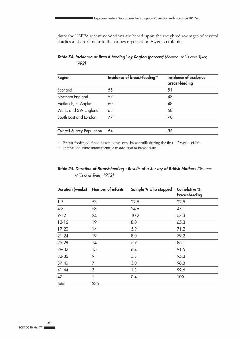
data; the USEPA recommendations are based upon the weighted averages of severalstudies and are similar to the values reported for Swedish infants.

Table 54. Incidence of Breast-feeding* by Region (percent) (Source: Mills and Tyler,1992)

Region Incidence of breast-feeding** Incidence of exclusivebreast-feeding

Scotland 55 51

Northern England 57 43

Midlands, E. Anglia 60 48

Wales and SW England 63 58

South East and London 77 70

Overall Survey Population 64 55

* Breast-feeding defined as receiving some breast milk during the first 1-2 weeks of life** Infants fed some infant formula in addition to breast milk

Table 55. Duration of Breast-feeding - Results of a Survey of British Mothers (Source:Mills and Tyler, 1992)

Duration (weeks) Number of infants Sample % who stopped Cumulative %breast-feeding

1-3 53 22.5 22.5

4-8 58 24.6 47.1

9-12 24 10.2 57.3

13-16 19 8.0 65.3

17-20 14 5.9 71.2

21-24 19 8.0 79.2

25-28 14 5.9 85.1

29-32 15 6.4 91.5

33-36 9 3.8 95.3

37-40 7 3.0 98.3

41-44 3 1.3 99.6

47 1 0.4 100

Total 236

86


ECETOC TR No. 79

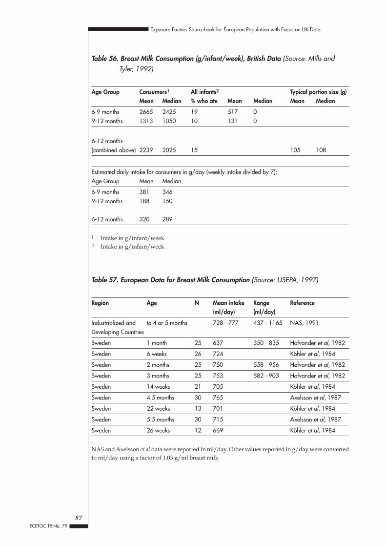
Table 56. Breast Milk Consumption (g/infant/week), British Data (Source: Mills andTyler, 1992)

Age Group Consumers1 All infants2 Typical portion size (g)Mean Median % who ate Mean Median Mean Median

6-9 months 2665 2425 19 517 09-12 months 1313 1050 10 131 0

6-12 months (combined above) 2239 2025 15 105 108

Estimated daily intake for consumers in g/day (weekly intake divided by 7):Age Group Mean Median

6-9 months 381 3469-12 months 188 150

6-12 months 320 289

1 Intake in g/infant/week2 Intake in g/infant/week

Table 57. European Data for Breast Milk Consumption (Source: USEPA, 1997)

Region Age N Mean intake Range Reference(ml/day) (ml/day)

Industrialized and to 4 or 5 months 728 - 777 437 - 1165 NAS, 1991Developing Countries

Sweden 1 month 25 637 350 - 835 Hofvander et al, 1982

Sweden 6 weeks 26 724 Köhler et al, 1984

Sweden 2 months 25 750 558 - 956 Hofvander et al, 1982

Sweden 3 months 25 753 582 - 903 Hofvander et al, 1982


Sweden 4.5 months 30 765 Axelsson et al, 1987


Sweden 5.5 months 30 715 Axelsson et al, 1987


NAS and Axelsson et al data were reported in ml/day. Other values reported in g/day were convertedto ml/day using a factor of 1.03 g/ml breast milk

87


ECETOC TR No. 79

Table 58. Breast Milk Intake Rates for US Breast-fed Infants (Source: USEPA, 1997)

USEPA 1997 Recommended Breast Milk Intake ValuesAge Mean (ml/day)* Upper percentile

(mean + 2 std dev.)

1-6 months 742 103312 month average 688 980

Detailed Data:Age N Mean (ml/day)* Upper percentile Reference

(mean + 2 std dev.)

1 month 11 600 918 Pao et al, 198037 729 981 Butte et al, 198413 747 1095 Neville et al, 198816 673 1057 Dewey and Lönnerdal, 1983Weighted Mean 702

3 months 2 833 ... Pao et al, 198037 702 923 Butte et al, 198412 712 934 Neville et al, 198816 782 1126 Dewey and Lönnerdal, 198373 788 1046 Dewey et al, 1991bWeighted Mean 759

6 months 1 682 ... Pao et al, 198013 744 978 Neville et al, 198811 896 1140 Dewey and Lönnerdal, 198360 747 1079 Dewey et al, 1991bWeighted Mean 765

9 months 12 600 1027 Neville et al, 198850 627 1049 Dewey et al, 1991bWeighted Mean 622

12 months 9 391 877 Neville et al, 198842 435 923 Dewey et al, 1991a; 1991bWeighted Mean 427

* Consumption in g/day converted to ml/day using the factor of 1.03 g/ml breast milk

88


ECETOC TR No. 79

6. DATA GAPS

While this document includes data for European countries in general, its primary focusis on the UK. Future expansion of additional data for other countries would be usefulfor improving the accuracy of exposure assessments for other European populations.

Data, from any country, are limited for both soil ingestion and soil adherence to skin.Additional studies are needed to quantify better these exposure factors.

Distributions are available for US time-activity data and food consumption rates, butdistributional data are not available for European populations. UK time-activity dataare limited even for point estimates of average or median values. Archived data fromUK time-activity and food consumption surveys may be recorded in sufficient detail todevelop distributions. Time-activity and food consumption surveys have been identifiedfor some non-UK European countries, but the level of detail for records of these studieswas not evaluated.

Inhalation rate data specific to the UK or Europe were not identified, and US data wereinsufficient to develop distributions. Other data not identified for the UK or Europeincluded shower duration, occupational tenure, and residential tenure.

89


ECETOC TR No. 79

ACKNOWLEDGEMENTS

This document represents a project developed from collaboration fostered by the Networkfor Industrially Contaminated Land in Europe (NICOLE).

Financial support was provided by ExxonMobil, ICI, and Shell.

The following are acknowledged for their contributions to the document’s preparation:

Authors

Rosemary Zaleski and Larry Gephart

Steering Committee and Peer Review

Jane Alcock, Martin Bell, Rae Crawford, William Hafker, Jane Lawson, and GordonLethbridge

Peer Review

Marie Amoruso, Stephen Bowes, Naomi Earl, Annette Guiseppi-Elie, Chris Money, andJoan Tell

Data Searches

Rengin Konuk

ECETOC Staff Scientist

Martin Holt

90


ECETOC TR No. 79

BIBLIOGRAPHY

American Industrial Health Council. 1994. Exposure Factors Sourcebook. American IndustrialHealth Council, Washington, DC, USA.

American Society for Testing and Materials (ASTM). 1995. Standard guide for risk-basedcorrective action applied at petroleum release sites. E1739-95e1. American Society for Testingand Materials, West Conshohocken, PA, USA.

American Society for Testing and Materials (ASTM). 1998. Standard provisional guide forrisk-based corrective action. PS104-98. American Society for Testing and Materials, WestConshohocken, PA, USA.

Andersen NL, Fagt S, Groth MV, Hartkopp HB, Moller A, Ovesen L, Warming DL. 1996.Danish diet survey 1995. Main results. Levnedsmiddelstyrelsen No. 235, Soborg, Denmark.

Axelsson I, Borulf S, Righard L, Räihä N. 1987. Protein and energy intake during weaning:effects and growth. Acta Paediatr Scand 76:321-327.

Binder S, Sokal D, Maughan D. 1986. Estimating the amount of soil ingested by young childrenthrough tracer elements. Arch Environ Health 41:341-345.

Boyd E. 1935. The growth of the surface area of the human body. University of MinnesotaPress, Minneapolis, MN, USA.

Burmaster DE. 1998a. Lognormal distributions for skin area as a function of body weight.Risk Analysis 18:27-32.

Burmaster DE. 1998b. A lognormal distribution for time spent showering. Risk Analysis 18:33-36.

Burmaster DE, Anderson PD. 1994. Principles of good practice for the use of Monte Carlotechniques in human health and ecological risk assessments. Risk Analysis 14: 477-481.

Burmaster DE, Crouch EAC. 1997. Lognormal distributions for body weight as a functionof age for males and females in the United States, 1976-1980. Risk Analysis 17:499-505.

Burmaster DE, von Stackelberg K. 1991. Using Monte Carlo simulations in public health riskassessments: estimating and presenting full distributions in risk. J Expos Anal Environ Epidemiol1:491-512.

Butte NF, Garza C, Smith EO, Nichols BL. 1984. Human milk intake and growth in exclusivelybreast-fed infants. J Pediatrics 104:187-195.

Calabrese EJ, Barnes R, Stanek EJ, Pastides H, Bilbert CE, Veneman P, Wang X, Laszity A,Kostecki PT. 1989. How much soil do young children ingest: an epidemiological study. RegulToxicol Pharm 10:123-139.

Calabrese EJ, Stanek EJ, Gilbert CE, Barnes RM. 1990. Preliminary adult soil ingestionestimates: Results of a pilot study. Regul Toxicol Pharm 12:88-95.

91


ECETOC TR No. 79

Calabrese EJ, Stanek EJ. 1991. A guide to interpreting soil ingestion studies. 2. Qualitativeand quantitative evidence of soil ingestion. Regul Toxicol Pharm 13:278-292.

Calabrese EJ, Stanek EJ. 1992. What proportion of household dust is derived from outdoorsoil. J Soil Contam 1:253-263.

Calabrese EJ, Stanek EJ. 1993. An improved method for estimating soil ingestion in childrenand adults. J Environ Sci Health A28:363-371.

Calabrese EJ, Stanek EJ. 1995. Resolving inter-tracer inconsistencies in soil ingestion estimates.Environ Health Perspectives 103:454-457.

Calabrese EJ, Stanek EJ, Pekow P, Barnes RM. 1997. Soil ingestion estimates for childrenresiding on a Superfund site. Ecotox Environ Saf 36:358-268.

CARACAS. 1998. Risk assessment for contaminated sites in Europe. Volume 1: Scientificbasis, and Volume 2: Policy frameworks. A report prepared as part of the Concerted Actionon Risk Assessment for Contaminated Sites in the European Union (CARACAS). LQM Press,Nottingham, UK.

Chambolle M, Volatier J-L, Combris P. 1995. L’observatoire des consommations alimentaires:objectifs, méthodes et réalisations. Cahiers de Nutrition et de Diététique 30: 279-386.

Clausing PB, Brunekreff PB, van Wijnen JH. 1987. A method for estimating soil ingestionin children. Int Arch Occup Environ Med 59:73.

CONCAWE. 1997. European oil industry guideline for risk-based assessment of contaminatedsite. Report no. 2/97, Prepared for the CONCAWE Water Quality Management Group byits Special Task Force (WQ/STF-27), based upon work performed under contract toCONCAWE by Dames and Moore.

Costeff H. 1966. A simple empirical formula for calculating approximate surface area inchildren. Arch Dis Child 41:681-683.

Davies PSW. 1997. Diet composition and body mass index in pre-school children. Eur JClin Nutr 51:443-448.

Davis S, Waller P, Buschom R, Ballou J, White P. 1990. Quantitative estimates of soil ingestionin normal children between the ages of 2 and 7 years. Population-based estimates usingaluminum, silicon, and titanium as soil tracer elements. Arch Environ Health 45:112-122.

Department for Education and Employment. 2000a. Information on primary and secondaryschool grades from website http://www.dfee.gov.uk/performance/primary_99/psec2.htm.

Department for Education and Employment. 2000b. Email correspondence from N. Chandler-Honnor.

Department for Education and Employment. 1999. Personal conversation with M. Patel.

Department of Education and Science. 1990. Management of the school day. Circular No.7/90. Elizabeth House, York Road, London, UK.

92


ECETOC TR No. 79

Dewey KG, Lönnerdal B. 1983. Milk and nutrient intake of breast-fed infants from 1 to 6months: relation to growth and fatness. Journal of Pediatric Gastroenterology and Nutrition2:497-506.

Dewey KG, Heinig J, Nommsen LA, Lönnerdal B. 1991a. Maternal versus infant factorsrelated to breast milk intake and residual volume: the DARLING study. Pediatrics 87:829-837.

Dewey KG, Heinig J, Nommsen LA, Lönnerdal B. 1991b. Adequacy of energy intake amongbreast-fed infants in the DARLING study: relationships to growth, velocity, morbidity,and activity levels. J Pediatrics 119:538-547.

Dubois D, Dubois EF. 1916. A formula to estimate the approximate surface area if height andweight be known. Arch Internal Med 17:863-871.

ECETOC. 1994. Assessment of non-occupational exposure to chemicals. Technical reportNo. 58. European Centre for Ecotoxicology and Toxicology of Chemicals, Brussels, Belgium.

ECETOC. 1995. Assessment factors in human health risk assessment. Technical report No.68. European Centre for Ecotoxicology and Toxicology of Chemicals, Brussels, Belgium.

Estívariz CF, López del Val T, Martínez P, Jansolo Barrenechea MA, De Cos Blanco AI,Cilleruelo Pascual ML, Vásquez Martínez C. 1996. Actual intake of milk products by apopulation of school children in the community of Madrid and their contribution of dietarynutrients. Anales Espanoles Pediatria 96:214-218.

Euromonitor. 1992. European Marketing and Statistics. ISBN: 0 86338 403 X, EuromonitorPlc 1992, used with permission.

Farrow A, Taylor H, Golding J. 1997. Time spent in the home by different family members.Environ Technol 18:605-614.

Gehan EA, George SL. 1970. Estimation of human body surface area from height and weight.Cancer Chemotherapy Reports 1:225-235.

Gershuny JI. 1985. Evaluation of 1983/84 ESRC Time Budget Data. ESRC End of grant report,for award no. GOO/23/2210. The Economic and Social Research Council, UK.

Gershuny JI. 1995. Establishing a British Centre for Time Budget Analysis. Economic andSocial Research Council End of Award Report, UK.

GIUDATTA ©. 1999. Version 1.1. Province of Milan and Dames and Moore International,s.r.l. Website: http://www.provincia.milano.it/progettispeciali.

Gregory JR, Collins DL, Davies PSW, Hughes JM, Clarke PC. 1995. National Diet and NutritionSurvery: children aged 1fi to 4fi years. Volume 1: Report of the diet and nutrition survey.HMSO, London, UK.

Gregory J, Foster K, Tyler H, Wiseman M. 1990. The Dietary and Nutritional Survey of BritishAdults. HMSO, London, UK.

93


ECETOC TR No. 79

Grigg D. 1993. The European diet: regional variations in food consumption in the 1980s.Geoforum 24:277-289.

Hackett AF, Kirby S, Howie M. 1997. A national survey of the diet of children aged 13-14years living in urban areas of the United Kingdom. J Hum Nutr and Diet 10:37-51.

Hamill PVV, Drizd TA, Johnson CL, Reed RB, Roche AF, Moore WM. 1979. Physical growth:National Center for Health Statistics percentiles. American Journal of Clinical Nutrition32:607-609.

Hawkins NC, Jayjock MA, Lynch J. 1992. A rationale and framework for establishing thequality of human exposure assessments. Am Ind Hyg Assoc J 53: 34-41.

Hoffman FO. 1993. Propagation of uncertainty in risk assessments: the need to distinguishbetween uncertainty due to lack of knowledge and uncertainty due to variability. USEPA/University of Virginia Workshop on When and How Can You Specify a ProbabilityDistribution When You Don't Know Much, University of Virginia, Charlottesville, VA, USA19-21 April 1993.

Hofmann W. 1982. Mathematical model for the postnatal growth of the human lung. RespirPhysiol 49:115-129.

Hofvander Y, Hagman U, Hillervik C, Sjolin S. 1982. The amount of milk consumed by 1 - 3 months old breast-or bottle-fed infants. Acta Paediatr Scand 71:953-958.

Holmes KK, Kissel JC, Richter KY. 1996. Investigation of the influence of oil on soil adherenceto skin. J Soil Contam 5: 301-308.

Hopkin SM, Ellis JC. 1980. Drinking water consumption in Great Britain: a survey of drinkinghabits with special reference to tap-water-based beverages. Technical Report 137, WaterResearch Centre, Wiltshire, UK.

Hulshof KFAM, Van Staveren WA. 1991. The Dutch National Food consumption survey:design, method and first results. Food Policy 16:257-260.

Ibrekk H, Morgan MG. 1983. Graphical communication of uncertain quantities to nontechnicalpeople. Risk Analysis 7:519-529.

Ihme W. 1994. Allgemeines Modell zur Quantifizierung der Exposition des Menschen durchkontaminierte Böden. D468 (Diss. Universität-GH Wuppertal). Verlag Shaker. ISBN 3-86111-859-9.

Israeli M, Nelson CB. 1992. Distribution and expected time of residence for U.S. households.Risk Analysis 12:65-72.

Jackson A, Edulgee G. 1996. Overview of risk assessment and its application. Chapter 1 ofEnvironmental Impact of Chemicals: Assessment and Controls, eds. Quint MD, Taylor R,Purchase R. The Royal Society of Chemistry, Cambridge, UK.

James IR, Knuiman MW. 1987. An application of Bayes methodology to the analysis of diaryrecords from a water use study. J Am Stat Assoc 832:705-711.

94


ECETOC TR No. 79

Johnson T, Capel J. 1992. A Monte Carlo approach to simulating residential occupancy periodsand its application to the general U.S. population. Research Triangle Park, NC, USA: USEPA,Office of Air Quality and Standards.

Jones PRM, Wilkinson S, Davies PSW. 1985. A revision of body surface area estimates. EuropeanJournal of Applied Physiology 58:376-379.

Kissel J, Richter K, Duff R, Fenske R. 1996a. Factors Affecting Soil Adherence to Skin Hand-Press Trials. Bull Environ Contamin Toxicol 56:722-728.

Kissel J, Richter K, Fenske R. 1996b. Field measurements of dermal soil loading attributableto various activities: Implications for exposure assessment. Risk Anal 16:116-125.

Köhler L, Meeuwisee G, Mortensson W. 1984. Food intake and growth of infants betweensix and twenty-six weeks of age on breast milk, cow’s milk formula and soy formula. ActaPaediatr Scand 73:40-48.

Layton DW 1993. Metabolically consistent breathing rates for use in dose assessment. HealthPhysics 64: 23-36.

Le Francois P, Calamassi-Tran G, Hebel P, Renault C, Lebreton S, Volatier JL. 1996. Food andnutrient intake outside the home of 629 French people of fifteen years and over. Eur J ClinNutr 50:826-831.

Martinchik AN, Baturin AK, Khel’singE, Charzhevska Y, Bondarev GI, Feoktistova AN,Zemlyanskaya TA, Azizbekyan TA, Baeva VS, Pyatnitskaya IN, Larina TI, Peskova EV,Lyndina MI, Zaburkina TG, Trofimenko LS. 1996. Monitoring of food intake and the nutritionalstate of Moscow children in 1992-4. 1. Methodology of investigation. Intakes of energyand nutrients. Voprosy Pitaniya 6:12-18.

Martonen TB, Graham RC, Hofmann W. 1989. Human subject age and activity level: factorsaddressed in a biomathematical deposition programme for extrapolation modeling. HealthPhysics 57:49.

McKone TE, Daniels JI. 1991. Estimating human exposure through multiple pathways fromair, water and soil. Regul Toxicol Pharm 13:36-61.

McNall PE, Schlegel JC. 1968. Practical thermal environmental limits for young adult malesworking in hot, humid environments. American Society of Heating, Refrigerating and Air-Conditioning Engineers (ASHRAE) Transactions 74:225-235.

Mills A, Tyler H. 1992. Food and nutrient intakes of British infants aged 6-12 months. HMSO,London, UK.

Ministry of Agriculture, Fisheries, and Food (MAFF). 1997. 1994 Total Diet Study- Nitrateand Nitrite. Food Surveillance Information Sheet Number 137, UK.

Murray DM, Burmaster DE. 1992. Estimated distributions for total body surface area of menand women in the United States. Journal of Exposure Analysis and Environmental Epidemiology2:451-461.

95


ECETOC TR No. 79

National Academy of Sciences (NAS). 1991. Nutrition during lactation. National AcademyPress. Washington, DC, USA.

National Center for Health Statistics (NCHS). 1987. Anthropometric reference data andprevalence of overweight, United States 1976-1980. Data from the National Health andNutrition Examination Survey, Series 11, No. 238. U.S. Department of Health and HumanServices, Public Health Service, National Center for Health Statistics. DHHS Publication No.(PHS) 87-1688. Hyattsville, MD, USA.

Neville MC, Keller R, Seacat J, Lutes V, Neifert M. 1988. Studies in human lactation: milkvolumes in lactating women during the onset of lactation and full lactation. American Journalof Clinical Nutrition 48:375-1386.

OECD. 1993. Employment Outlook. Organization for Economic Co-operation andDevelopment, Paris, France.

OECD. 1997. Labour Force Statistics: 1976-1996. Organization for Economic Co-operationand Development, Paris, France.

OECD. 1998a. Labour Force Statistics, 1977-1997. Organization for Economic Co-operationand Development, Paris, France.

OECD. 1998b. Employment Outlook. Organization for Economic Co-operation andDevelopment, Paris, France.

Ott WR. 1988. Human Activity Patterns: A review of the literature for estimating time spentindoors, outdoors, and in transit. Research Planning Conference on Human Activity Patterns,May 10-12 1988, Las Vegas, NV, USA.

Pao EM, Hines JM, Roche AF. 1980. Milk intakes and feeding patterns of breast-fed infants.Journal of the American Dietetic Association 77:540-545.

Paul AA, Black AE, Evans J, Cole TJ, Whitehead RG. 1988. Breastmilk intake and growthin infants from two to ten months. J Hum Nutr and Diet 1:437-450.

Payne JA, Belton NR. 1992. Nutrient intake and growth in pre-school children. Comparisonof energy intake and sources of energy with growth. J Hum Nutr and Diet 5:287-298.

Pérez-Llama F, Garaulet M, Nieto M, Baraza JC, Zamor S. 1996. Estimates of food intake anddietary habits in a random sample of adolescents in south-east Spain. J Hum Nutr and Diet9:463-471.

Prescott-Clarke P, Primatesta P. 1998a. The Health Survey for England 1996. The StationeryOffice. Adult body weight data at website www.official-documents.co.uk/document/doh/survey96/tab7-8.htm. Crown copyright.

Prescott-Clarke P, Primatesta P. 1998b. The Health of Young People ‘95-97. The StationeryOffice. Child body weight at website www.official-documents.co.uk/document/doh/survey97/hst3-3.htm. Crown copyright.

96


ECETOC TR No. 79

Quint MD, Taylor D, Purchase R. 1996. Environmental impact of chemicals: assessment andcontrol. Royal Society of Chemistry, Cambridge, UK.

Roels HA, Buchet JP, Lauwenys RR, Branx P, Claeys-Thoreau F, Lafontaine A, Verduyn G.1980. Exposure to lead by oral and pulmonary routes of children living in the vicinity of aprimary lead smelter. Environ Res 22:81-94.

Roy M., Becquemin MH, Bouchikhi A. 1991. Ventilation rates and lung volumes for lungmodelling purposes in ethnic groups. Radiation Protection Dosimetry 38:49-55.

Rusconi F, Catagento M, Gagliardi L, Gualtiero L, Pellegatta A, Port N, Razon S, Braga M.1994. Reference values for respiratory rate in the first 3 years of life. Pediatrics 94:350-355.

Schneider AT. 1995. Ergebnisse der Nationalen Verzehrsstudie (1985-1988) über Lebensmittel- und Nährstoffaufnahme in der Bundesrepublik Deutschland. Band IX. VERA-Schriftenreihe.Wissenschaftlicher Fachverlag Dr. Fleck, Niederkleen, Germany.

Simon SL. 1998. Soil ingestion by humans: a review of history, data, and etiology withapplication to risk assessment of radioactively contaminated soil. Health Physics 74: 647-672.

Slater J, Bolton-Smith C, Burns J, Chesher A, Church S, Platt S, Price R, Stainer T, WhiteheadR, Wiseman M, Speller S. 1998. National Food Survey 1997: Annual report on food expenditure,consumption and nutrient intakes. Ministry of Agriculture, Fisheries and Food (MAFF). TheStationery Office, London, UK.

Snyder WS, Cook MJ, Nasset ES, Karhausen LR, Parry Howells G, Tipton IH. 1975. Reportof the task group on reference man: a report prepared by a task group of committee 2 ofthe International Commission on Radiological Protection. ICRP Report No. 23. PergamonPress, Oxford, UK.

Stanek EJ, Calabrese EJ. 1991. A guide to interpreting soil ingestion studies. 1. Developmentof a model to estimate the soil ingestion detection level of soil ingestion studies. Regul ToxicolPharm 13:263-277.

Stanek EJ, Calabrese EJ. 1993. Soil ingestion in children. Outdoor soil or indoor dust?Hydrocarbon Contaminated Soils and Groundwater. Lewis Publishers. pp 519-545.

Stanek EJ, Calabrese EJ. 1994. Bias and the detection limit model for soil ingestion. J SoilContam 3:183-190.

Stanek EJ, Calabrese EJ. 1995. Improved soil ingestion estimated by the best tracer methodpaper. Human and Ecological Risk Assessment 1:133-156.

Stanek EJ, Calabrese EJ, Barnes R, Pekow P. 1997. Soil ingestion in adults: results of a secondpilot study. Ecotox Environ Saf 36:249-257.

United Kingdom Government Actuary’s Department. 1998. The Nations Health, TablesA1 and A2, from the Health and Personal Social Services Statistics information site atwww.doh.gov.uk/HPSSS/TBL_A1.HTM and A2.HTM. Crown copyright, used withpermission.

97


ECETOC TR No. 79

United Kingdom Office for National Statistics. 1998. Table 7.8 from the Health Survey forEngland 96, Adult’s weight, by age and sex. From website www.official-documents.co.uk/document/doh/survey96/tab7-8.htm. Crown copyright, used with permission.

United Kingdom Office for National Statistics. 1999a. Table 3.3 from The Health of YoungPeople ‘95-97, Weight, by age and sex. From website www.official-documents.co.uk/document/doh/survey97/hst3-3.htm. Crown copyright, used with permission.

United Kingdom Office for National Statistics. 1999b. Government Statistical Service - theSource of UK Facts and Figures. Average usual hours worked per person per week. Fromwebsite www.statistics.gov.uk/stats/ukinfigs/employ.htm. Crown copyright, used withpermission.

United Kingdom Office for National Statistics. 1999c. Government Statistical Service - theSource of UK Facts and Figures. Data set LFSEX2. All in employment by usual weekly hoursof work by gender. From website www.statistics.gov.uk/stats/statbase/ xsdataset.asp?list1=1&list2=1&B2=Display+All. Crown copyright, used with permission.

United States Environmental Protection Agency. 1989a. Exposure Factors Handbook, FinalReport. EPA/600/8-89/043, Office of Health and Environmental Assessment, Washington,DC, USA.

United States Environmental Protection Agency. 1989b. Risk assessment guidance forSuperfund, Vol. I. Human health evaluation manual (part A). EPA/540/1-89/002, Officeof Emergency and Remedial Response, Washington, DC, USA.

United States Environmental Protection Agency. 1992a. Guidelines for exposure assessment.Federal Register 57:22888-22938.

United States Environmental Protection Agency. 1992b. Dermal exposure assessment:Principles and Applications. EPA/600/8-91/011B. Office of Health and EnvironmentalAssessment, Washington, DC, USA.

United States Environmental Protection Agency. 1997a. Exposure Factors Handbook, VolumesI- III. EPA/600/P-95/002Fa,b,c.

United States Environmental Protection Agency. 1997b. Guiding principles for Monte Carloanalysis. EPA/630/R-97/001. Risk Assessment Forum, Washington, DC, USA.

United States Environmental Protection Agency. 2000. Risk assessment guidance forSuperfund: Volume 3 - (Part A, Process for conducting probabilistic risk assessment). Officeof Solid Waster and Emergency Response. Draft available from the USEPA website,www.epa.gov.

van de Ven-Breken TJ, Brenot J, Bonnefous S, Noordijk H, Leenhouts HP. 1990. Consumptionof food in EC countries CEC research programme Post Chernobyl Action 5: underlying datafor derived emergency reference levels. National Institute of Public Health and EnvironmentalProtection (RIVM), The Netherlands.

van Poppel G. 1998. Intake of trans fatty acids in western Europe: the TRANSFAIR study351:1099.

98


ECETOC TR No. 79

van Wijnen JH, Clausing P, Brunekreff B. 1990. Estimated soil ingestion by children. EnvironRes 51:147-162.

Vik EA, Breedveld G, Farestveit T. 1999. Guidelines for the risk assessment of contaminatedsites. Norwegian Pollution Control Authority (SFT), Report 99:06, Oslo, Norway.

Whichelow MJ, Erzinclioglu SW, Cox BD. 1991. Some regional variations in dietary patternsin a random sample of British adults. Eur J Clin Nutr 45:253-262.

World Health Organization. 1999a. WHO Global Database on Body Mass Index (BMI).

World Health Organization. 1999b. The World Health Report 1999. Basic Health Indicators,Annex Table 1. Available from http://www-nt.who.int/whosis/basic/ basicqueryprocess.cfm.

99


ECETOC TR No. 79

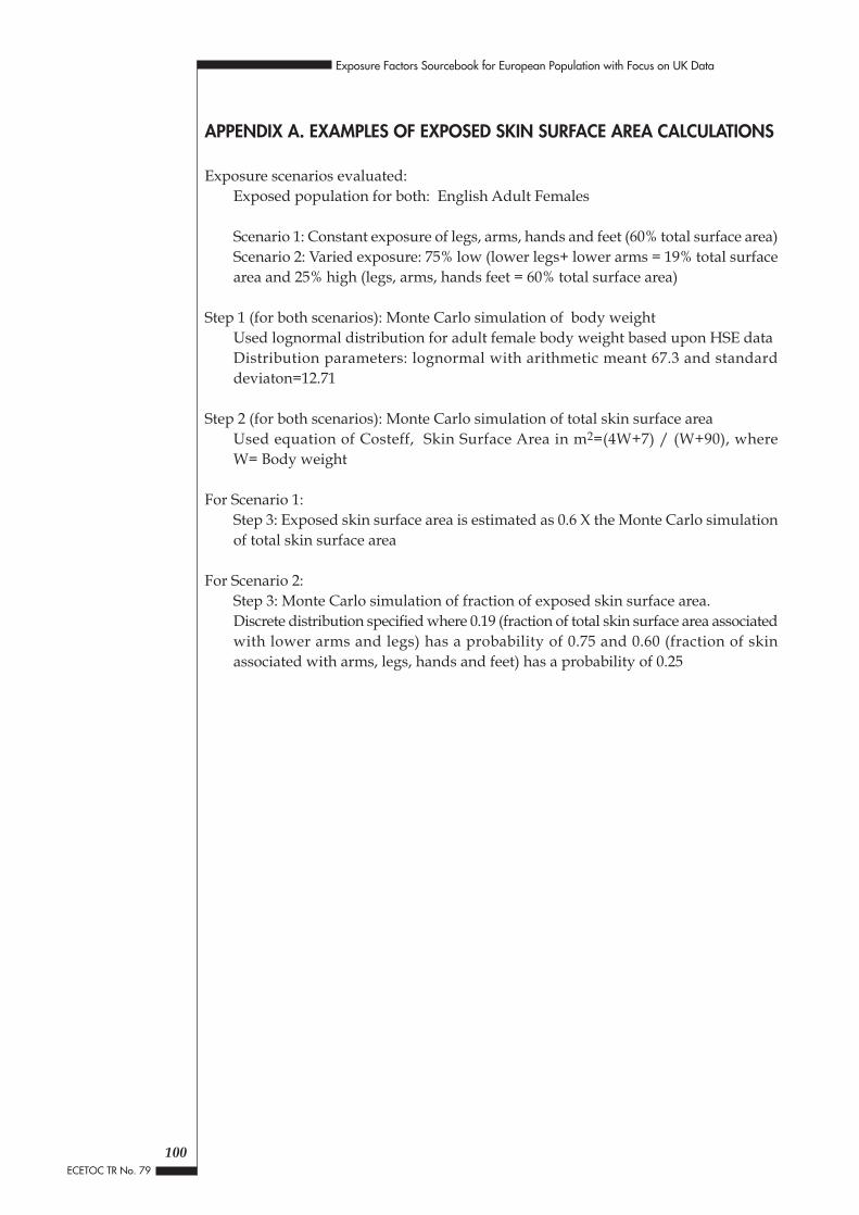
APPENDIX A. EXAMPLES OF EXPOSED SKIN SURFACE AREA CALCULATIONS

Exposure scenarios evaluated:Exposed population for both: English Adult Females

Scenario 1: Constant exposure of legs, arms, hands and feet (60% total surface area)Scenario 2: Varied exposure: 75% low (lower legs+ lower arms = 19% total surfacearea and 25% high (legs, arms, hands feet = 60% total surface area)

Step 1 (for both scenarios): Monte Carlo simulation of body weightUsed lognormal distribution for adult female body weight based upon HSE dataDistribution parameters: lognormal with arithmetic meant 67.3 and standarddeviaton=12.71

Step 2 (for both scenarios): Monte Carlo simulation of total skin surface areaUsed equation of Costeff, Skin Surface Area in m2=(4W+7) / (W+90), whereW= Body weight

For Scenario 1:Step 3: Exposed skin surface area is estimated as 0.6 X the Monte Carlo simulationof total skin surface area

For Scenario 2:Step 3: Monte Carlo simulation of fraction of exposed skin surface area.Discrete distribution specified where 0.19 (fraction of total skin surface area associatedwith lower arms and legs) has a probability of 0.75 and 0.60 (fraction of skinassociated with arms, legs, hands and feet) has a probability of 0.25

100


ECETOC TR No. 79

Crystal Ball Reports for Monte Carlo Simulations

Forecast: Adult Female Body Weight, Lognormal Simulation

SummaryDisplay Range is from 30.00 to 110.00Entire Range is from 32.33 to 123.84After 1,000 Trials, the Std. Error of the Mean is 0.44

Statistics Value

Trials 1000

Mean 67.92

Median 66.51

Mode ---

Std Dev. 13.80

Variance 190.35

Skewness 0.58

Kurtosis 3.73

Coeff. of Variability 0.20

Range Minimum 32.33

Range Maximum 123.84

Range Width 91.51

Mean Std. Error 0.44



101


ECETOC TR No. 79

Forecast: Adult Female Body Weight, Lognormal Simulation (continued)

Percentiles:

Percentile Value

0% 32.33

5% 46.98

10% 51.78

15% 54.17

20% 56.20

25% 58.36

30% 59.86

35% 61.77

40% 63.52

45% 64.75

50% 66.51

55% 68.38

60% 70.16

65% 72.05

70% 74.25

75% 76.43

80% 78.66

85% 81.34

90% 86.59

95% 92.98

100% 123.84

End of Forecast

102


ECETOC TR No. 79

Forecast: Adult Female Skin Surface Area - Costeff Equation

SummaryDisplay Range is from 1.20 to 2.30Entire Range is from 1.11 to 2.35 After 1,000 Trials, the Std. Error of the Mean is 0.01

Statistics Value

Trials 1000

Mean 1.75

Median 1.74

Mode ---

Std Dev. 0.19

Variance 0.04

Skewness 0.02

Kurtosis 3.08


Range Minimum 1.11

Range Maximum 2.35

Range Width 1.23


Forecast: Adult Female Skin Surface Area - Costeff Equation

103


ECETOC TR No. 79

Forecast: Adult Female Skin Surface Area - Costeff Equation (continued)

Percentiles:

Percentile Value

0% 1.11

5% 1.42

10% 1.51

15% 1.55

20% 1.59

25% 1.62

30% 1.64

35% 1.67

40% 1.70

45% 1.72

50% 1.74

55% 1.77

60% 1.80

65% 1.82

70% 1.85

75% 1.88

80% 1.91

85% 1.94

90% 2.00

95% 2.07

100% 2.35

End of Forecast

104


ECETOC TR No. 79

Forecast: Adult Female Exposed SSA, Constant 60% Exposure

SummaryDisplay Range is from 0.75 to 1.35Entire Range is from 0.67 to 1.41After 1,000 Trials, the Std. Error of the Mean is 0.00

Statistics Value

Trials 1000

Mean 1.05

Median 1.05

Mode ---

Std Dev. 0.12

Variance 0.01

Skewness 0.02

Kurtosis 3.08


Range Minimum 0.67

Range Maximum 1.41

Range Width 0.74


Forecast: Adult Female Exposed SSA, Constant 60% Exposure

105


ECETOC TR No. 79

Forecast: Adult Female Exposed SSA, Constant 60% Exposure (continued)

Percentiles:

Percentile Value

0% 0.67

5% 0.85

10% 0.91

15% 0.93

20% 0.95

25% 0.97

30% 0.99

35% 1.00

40% 1.02

45% 1.03

50% 1.05

55% 1.06

60% 1.08

65% 1.09

70% 1.11

75% 1.13

80% 1.14

85% 1.16

90% 1.20

95% 1.24

100% 1.41

End of Forecast

106


ECETOC TR No. 79

Forecast: Varied Exposure - Fraction Exposed (75% Low, 25% High)

SummaryDisplay Range is from 0.15 to 0.60 percent exposedEntire Range is from 0.19 to 0.60 percent exposedAfter 1,000 Trials, the Std. Error of the Mean is 0.01

Statistics Value

Trials 1000

Mean 0.28

Median 0.19

Mode 0.19

Std Dev. 0.17

Variance 0.03

Skewness 1.31

Kurtosis 2.71


Range Minimum 0.19

Range Maximum 0.60

Range Width 0.41


End of Forecast

Forecast: Varied Exposure (75% Low, 25% High)

107


ECETOC TR No. 79

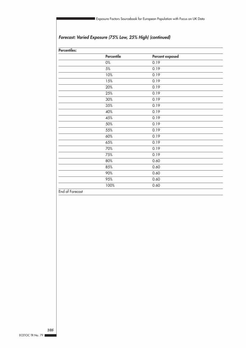
Forecast: Varied Exposure (75% Low, 25% High) (continued)

Percentiles:

Percentile Percent exposed

0% 0.19

5% 0.19

10% 0.19

15% 0.19

20% 0.19

25% 0.19

30% 0.19

35% 0.19

40% 0.19

45% 0.19

50% 0.19

55% 0.19

60% 0.19

65% 0.19

70% 0.19

75% 0.19

80% 0.60

85% 0.60

90% 0.60

95% 0.60

100% 0.60

End of Forecast

108


ECETOC TR No. 79

Forecast: Adult Female Exposed SSA, Varied Exposure

SummaryDisplay Range is from 0.20 to 1.30 square metersEntire Range is from 0.21 to 1.39 square metersAfter 1,000 Trials, the Std. Error of the Mean is 0.01

Statistics Value

Trials 1000

Mean 0.49

Median 0.35

Mode ---

Std Dev. 0.31

Variance 0.09

Skewness 1.39

Kurtosis 3.17


Range Minimum 0.21

Range Maximum 1.39

Range Width 1.18


Forecast: Adult Female Exposed SSA, Varied Exposure

109


ECETOC TR No. 79

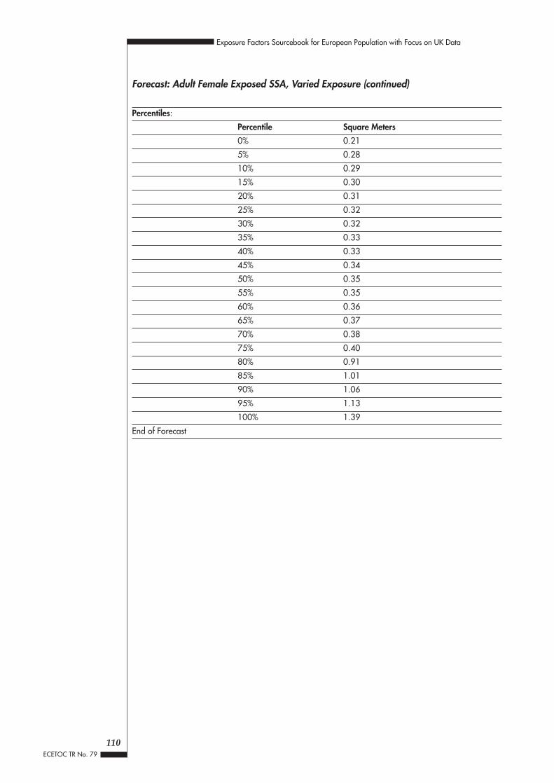
Forecast: Adult Female Exposed SSA, Varied Exposure (continued)

Percentiles:

Percentile Square Meters

0% 0.21

5% 0.28

10% 0.29

15% 0.30

20% 0.31

25% 0.32

30% 0.32

35% 0.33

40% 0.33

45% 0.34

50% 0.35

55% 0.35

60% 0.36

65% 0.37

70% 0.38

75% 0.40

80% 0.91

85% 1.01

90% 1.06

95% 1.13

100% 1.39

End of Forecast

110


ECETOC TR No. 79

APP

ENDI

X B.

PO

TEN

TIA

L SO

URC

ES O

F A

DDIT

ION

AL

INFO

RMAT

ION

FO

R RE

GIO

N S

PECI

FIC

EXPO

SURE

FA

CTO

RS

Publ

icat

ion

Refe

renc

eTy

pe o

f Inf

orm

atio

n In

clud

edCo

mm

ents

Purc

hase

Sou

rce

Pric

eEu

rope

an M

arke

ting

Dat

a an

dLif

e ex

pect

ancy

at b

irth;

pop

ulat

ion

by a

ge g

roup

; ave

rage

wor

king

Not

spe

cifie

d if

aver

age

valu

esEu

rom

onito

r£1

85,

Stat

istic

s, 1

999

wee

k in

non

-agr

icul

tura

l act

iviti

es 1

977-

94, a

vera

ge w

orki

ng w

eek

inor

dist

ribut

ions

are

pro

vide

d(w

ww

.eur

omon

itor.c

om)

US$

370

man

ufac

turin

g 19

77-9

5; e

cono

mic

ally

act

ive

popu

latio

n by

age

gro

up;

1996

per

cap

ita c

onsu

mpt

ion

of m

eat a

nd fi

sh, f

resh

pro

duce

, dai

rypr

oduc

ts an

d eg

gs, b

aker

y pr

oduc

ts, c

onve

nien

ce a

nd m

iscel

lane

ous

food

s, s

nack

food

s an

d ho

t drin

ks; p

rodu

ctio

n of

mea

t, ce

real

, sel

ecte

dcr

ops,

fish

ery

prod

ucts;

indi

ces

of a

gric

ultu

ral a

nd fo

od o

utpu

tW

orld

Mar

ketin

g D

ata

and

Sim

ilar t

o ab

ove,

but

for w

orld

not

just

Euro

pe a

nd s

ome

data

are

Not

spe

cifie

d if

aver

age

valu

esEu

rom

onito

r£7

95,

Stat

istic

s, 1

999

mor

e cu

rren

t (i.e

. foo

d co

nsum

ptio

n da

ta a

re fo

r 199

7, w

eekl

yor

dist

ribut

ions

are

pro

vide

d(w

ww

.eur

omon

itor.c

om)

US$

2100

wor

k ho

urs

are

thro

ugh

1997

)G

arde

ning

in E

urop

eTr

ends

in g

arde

n ow

ners

hip,

cha

ngin

g le

isure

pat

tern

s, g

arde

nSp

ecifi

city

of d

ata

not p

rovi

ded

Euro

mon

itor

£395

0,m

arke

ting

by s

ecto

r by

coun

try, p

opul

atio

n tre

nds

(i.e.

- gar

deni

ng in

clud

es la

wns

(ww

w.e

urom

onito

r.com

)U

S$79

00an

d or

nam

enta

l, no

t jus

t foo

dpr

oduc

tion)

; not

spe

cifie

d if

aver

age

valu

es o

r dist

ribut

ions

are

prov

ided

Con

sum

er L

ifesty

les

in

Hou

sing

trend

s, fo

od c

onsu

mpt

ion,

atte

ndan

ce a

t lei

sure

ven

ues

Not

spe

cifie

d if

aver

age

valu

esEu

rom

onito

r£8

95,

Easte

rn E

urop

eby

type

or d

istrib

utio

ns a

re p

rovi

ded

(ww

w.e

urom

onito

r.com

)U

S$17

90G

ener

al H

ouse

hold

Sur

vey.

Sam

pled

pop

ulat

ion:

priv

ate

hous

ehol

ds in

Brit

ain;

hou

sing

and

Not

spe

cifie

d if

aver

age

valu

esTh

e St

atio

nery

Offi

ce,

Livin

g in

Brit

ain:

resu

lts fr

omm

igra

tion;

job

mob

ility

; edu

catio

nal a

ctiv

ityor

dist

ribut

ions

are

pro

vide

dLo

ndon

; Uni

vers

ity o

f Ess

exth

e 19

95 G

ener

al H

ouse

hold

Dat

a A

rchi

ves

(Biro

n ca

talo

gSu

rvey

. Offi

ce o

f Nat

iona

l, nu

mbe

r 330

90)

Stat

istic

s So

cial

Sur

vey

Div

ision

. 199

7

111


ECETOC TR No. 79

112


ECETOC TR No. 79

APP

ENDI

X B.

CO

NTI

NU

ED

Publ

icat

ion

Refe

renc

eTy

pe o

f Inf

orm

atio

n In

clud

edCo

mm

ents

Purc

hase

Sou

rce

Pric

eBr

itish

Hou

seho

ld P

anel

Sur

vey

Sam

pled

pop

ulat

ion:

hou

seho

lds

in B

ritai

n an

d in

divi

dual

hou

seho

ldN

ot s

peci

fied

if av

erag

e va

lues

ESRC

Res

earc

h C

entre

on

Com

bine

d W

ork-

Life

Hist

ory

mem

bers

; occ

upat

iona

l hist

ory

or d

istrib

utio

ns a

re p

rovi

ded;

Mic

ro-S

ocia

l Cha

nge

(par

tD

ata,

199

0-19

95ra

w d

ata

are

avai

labl

e bu

tof

the

Insti

tute

for S

ocia

l and

user

nee

ds to

kno

w c

odes

Ec

onom

ic R

esea

rch;

Uni

vers

ity(a

ltern

ativ

ely,

for a

fee,

of E

ssex

Dat

a A

rchi

ves

(Biro

nan

alys

es c

an b

e pe

rfor

med

)ca

talo

g nu

mbe

r 331

96)

Fam

ily, w

ork

and

leisu

re in

Mai

n stu

dy: A

dult

popu

latio

n of

Lon

don

met

ropo

litan

regi

on. D

ate

Dat

ed, L

ondo

n ad

ults

only

;U

nive

rsity

of E

ssex

Dat

ath

e Lo

ndon

regi

onof

firs

t rel

ease

: 197

3; h

ours

at w

ork,

leisu

re a

ctiv

ities

by

hom

e no

t spe

cifie

d if

aver

age

Arc

hive

s (B

iron

Cat

alog

base

d or

oth

er. D

iarie

s fo

r mar

ried

resp

onde

nts

betw

een

ages

va

lues

or d

istrib

utio

ns

num

ber 3

3155

)of

30-

49 a

lso o

n re

cord

are

prov

ided

UK

Banb

ury

Act

ivity

/Po

pula

tion:

def

ined

sec

tor o

f Ban

bury

, N=2

04 h

ouse

hold

s.N

ot s

peci

fied

if av

erag

e va

lues

CES

SDA

Inte

grat

ed

Trav

el S

urve

y Se

pt-O

ct 1

976,

dia

ries

of a

ctiv

ities

with

loca

tion

or d

istrib

utio

ns a

re p

rovi

ded;

Dat

a C

atal

ogra

w d

ata

are

avai

labl

e(h

ttp:/

/das

tar.e

ssex

.ac.

uk),

(UK

data

arc

hive

num

ber

1095

)U

K N

orth

ern

Irela

nd H

ealth

Nor

ther

n Ire

land

adu

lts (>

16 y

rs),

N=1

200;

ass

ocia

ted

repo

rts:

Not

spe

cifie

d if

aver

age

valu

esC

ESSD

A In

tegr

ated

and

Act

ivity

Sur

vey,

199

4M

acA

uley

, D.,

et a

l199

4. N

orth

ern

Irela

nd H

ealth

and

Act

ivity

or d

istrib

utio

ns a

re p

rovi

ded;

Dat

a C

atal

ogSu

rvey

Rep

ort (

Belfa

st:H

MSO

); Ke

lly, F

. and

S. O

gle.

1994

. Nor

ther

nra

w d

ata

are

avai

labl

e(h

ttp:/

/das

tar.e

ssex

.ac.

uk),

Irela

nd H

ealth

and

Act

ivity

Sur

vey

Mai

n Fi

ndgi

ns (B

elfa

st:H

MSO

)(U

K da

ta a

rchi

ve n

umbe

r34

69)

UK

ESRC

/Man

ches

ter

Hou

seho

ld h

eads

age

d 20

-60

year

s in

six

war

ds o

f Mac

cles

field

,Ra

w d

ata

are

avai

labl

eC

ESSD

A In

tegr

ated

Uni

vers

ity M

accl

esfie

ldN

=669

, Nov

-Dec

198

3; o

ccup

atio

n, li

fe a

nd w

ork

histo

ries,

Dat

a C

atal

ogSu

rvey

, 198

3ho

me-

grow

n fo

ods

(key

wor

d un

der e

mpl

oym

ent o

ppor

tuni

ty),

(http

://d

asta

r.ess

ex.a

c.uk

),le

isure

tim

e ac

tiviti

es(U

K da

ta a

rchi

ve n

umbe

r25

59)

113


ECETOC TR No. 79

APP

ENDI

X B.

CO

NTI

NU

ED

Publ

icat

ion

Refe

renc

eTy

pe o

f Inf

orm

atio

n In

clud

edCo

mm

ents

Purc

hase

Sou

rce

Pric

eN

ew C

rono

s da

taba

seM

acro

econ

omic

and

soc

ial d

atab

ase

for t

he E

U M

embe

r Sta

tes

and

inRa

w d

ata

are

avai

labl

eEu

rosta

t Dat

a Sh

opEC

U 8

000,

man

y ca

ses,

Jap

an, t

he U

S, a

nd th

e ce

ntra

l Eur

opea

n co

untri

es a

ndca

n re

ques

tm

ain

econ

omic

par

tner

s of

the

EU; l

abou

r for

ce s

urve

y, p

opul

atio

npr

ices

for

surv

eys,

agr

icul

tura

l sur

veys

indi

vidu

alm

ains

colle

ctio

nsor

tabl

esLe

isure

Tre

nds

1998

Hob

bies

and

spo

rt, g

arde

ning

; ano

ther

leisu

re re

fere

nce

gave

Dat

a fo

rmat

unk

now

n, d

on't

Min

tel (

ww

w.m

inte

l.co.

uk),

£137

frequ

ency

of l

eisu

re a

ctiv

ities

by

loca

tion

but n

ot d

urat

ion

of e

ach

know

if v

alue

s re

leva

nt to

Mar

ketin

g In

telli

genc

efre

quen

cy, a

noth

er g

arde

ning

refe

renc

e gi

ves

dem

ogra

phic

expo

sure

ass

essm

ent,

such

as

cons

umer

mar

ket r

esea

rch

info

rmat

ion

abou

t gar

den

owne

rshi

p bu

t uns

ure

if da

ta a

re s

peci

fictim

e sp

ent a

t var

ious

loca

tions

,to

veg

etab

le o

r fru

it ga

rden

s vs

. law

n an

d or

nam

enta

l gar

dens

or %

of f

amili

es w

ith v

eget

able

gard

ens

MEMBERS OF THE ECETOC SCIENTIFIC COMMITTEE

(Peer Review Committee)

N. Carmichael (Co-chairman) AventisHead, Toxicology F - Sophia Antipolis

G. Randall (Co-chairman) AstraZenecaDirector, Environmental Laboratory UK - Brixham

C. Braun Akzo NobelOccupational Toxicologist NL - Arnhem

E. Bomhard BayerHead, Industrial Toxicology D - Wuppertal

C. d’Hondt SyngentaHead, Environmental Safety Department CH - Basel

T. Feijtel* Procter & GambleManager, Professional and Regulatory Services B - Brussels

J. Jackson MonsantoSenior Associate, Medical Adviser B - Brussels

R. Millischer AtofinaHead, Industrial Toxicology Department F - Paris

A. Sarrif DuPontDirector, Toxicology Affairs, Europe D - Bad Homburg

J. Solbé UnileverHead, SEAC Environment UK - Bebington

L. Smith* SyngentaDirector, Central Toxicology Laboratory UK - Macclesfield

B. van Raavenzwaay BASFDirector, Experimental Toxicology and Ecology D - Ludwigsafen

H-J. Wiegand DegussaHead, Product Safety Department D - Marl

114


ECETOC TR No. 79

* Stewards responsible for primary peer review

ECETOC PUBLISHED REPORTS

Monographs

No. Title

No. 1 Good Laboratory PracticeNo. 2 A Contribution to Strategy for Identification and Control of Occupational CarcinogensNo. 3 Risk Assessment of Occupational Chemical CarcinogensNo. 4 Hepatocarcinogenesis in Laboratory Rodents: Relevance for ManNo. 5 Identification and Assessment of the Effects of Chemicals on Reproduction and Development

(Reproductive Toxicology)No. 6 Acute Toxicity Tests, LD50 (LC50) Determinations and AlternativesNo. 7 Recommendations for the Harmonisation of International Guidelines for Toxicity StudiesNo. 8 Structure-Activity Relationships in Toxicology and Ecotoxicology: An Assessment (Summary)No. 9 Assessment of Mutagenicity of Industrial and Plant Protection ChemicalsNo. 10 Identification of Immunotoxic Effects of Chemicals and Assessment of their Relevance to

ManNo. 11 Eye Irritation TestingNo. 12 Alternative Approaches for the Assessment of Reproductive Toxicity (with emphasis on

embryotoxicity/teratogenicity)No. 13 DNA and Protein Adducts: Evaluation of their Use in Exposure Monitoring and Risk

AssessmentNo. 14 Skin Sensitisation TestingNo. 15 Skin IrritationNo. 16 Early Indicators of Non-Genotoxic CarcinogenesisNo. 17 Hepatic Peroxisome ProliferationNo. 18 Evaluation of the Neurotoxic Potential of ChemicalsNo. 19 Respiratory AllergyNo. 20 Percutaneous AbsorptionNo. 21 Immunotoxicity: Hazard Identification and Risk CharacterisationNo. 22 Evaluation of Chemicals for OculotoxicityNo. 23 Receptor Mediated Mechanisms in Chemical CarcinogenesisNo. 24 Risk Assessment for CarcinogensNo. 25 Practical Concepts for Dose Selection in Chronic Toxicity and Carcinogenicity Studies in

RodentsNo. 26 Aquatic Toxicity Testing of Sparingly Soluble Volatile and Unstable SubstancesNo. 27 AneuploidyNo. 28 Threshold-Mediated Mutagens - Mutation Research Special IssueNo. 29 Skin Sensitisation Testing for the Purpose of Hazard Identification and Risk Assessment

Technical Reports

No. Title

No. 1 Assessment of Data on the Effects of Formaldehyde on HumansNo. 2 The Mutagenic and Carcinogenic Potential of FormaldehydeNo. 3 Assessment of Test Methods for Photodegradation of Chemicals in the EnvironmentNo. 4 The Toxicology of Ethylene Glycol Monoalkyl Ethers and its Relevance to ManNo. 5 Toxicity of Ethylene Oxide and its Relevance to ManNo. 6 Formaldehyde Toxicology: An Up-Dating of ECETOC Technical Reports 1 and 2No. 7 Experimental Assessment of the Phototransformation of Chemicals in the Atmosphere

115


ECETOC TR No. 79

No. 8 Biodegradation Testing: An Assessment of the Present StatusNo. 9 Assessment of Reverse-Phase Chromatographic Methods for Determining Partition CoefficientsNo. 10 Considerations Regarding the Extrapolation of Biological Data in Deriving Occupational

Exposure LimitsNo. 11 Ethylene Oxide Toxicology and its Relevance to Man: An Up-Dating of ECETOC Technical

Report No. 5No. 12 The Phototransformation of Chemicals in Water: Results of a Ring-Test No. 13 The EEC 6th Amendment: A Guide to Risk Evaluation for Effects on the EnvironmentNo. 14 The EEC 6th Amendment: A Guide to Risk Evaluation for Effects on Human HealthNo. 15 The Use of Physical-Chemical Properties in the 6th Amendment and their Required Precision,

Accuracy and Limiting ValuesNo. 16 A Review of Recent Literature on the Toxicology of BenzeneNo. 17 The Toxicology of Glycol Ethers and its Relevance to Man: An Up-Dating of ECETOC Technical

Report No. 4No. 18 Harmonisation of Ready Biodegradability TestsNo. 19 An Assessment of Occurrence and Effects of Dialkyl-o-Phthalates in the EnvironmentNo. 20 Biodegradation Tests for Poorly-Soluble CompoundsNo. 21 Guide to the Classification of Carcinogens, Mutagens, and Teratogens under the 6th

AmendmentNo. 22 Classification of Dangerous Substances and Pesticides in the EEC Directives. A Proposed

Revision of Criteria for Inhalational ToxicityNo. 23 Evaluation of the Toxicity of Substances to be Assessed for BiodegradabilityNo. 24 The EEC 6th Amendment: Prolonged Fish Toxicity TestsNo. 25 Evaluation of Fish TaintingNo. 26 The Assessment of Carcinogenic Hazard for Human Beings exposed to Methylene ChlorideNo. 27 Nitrate and Drinking WaterNo. 28 Evaluation of Anaerobic BiodegradationNo. 29 Concentrations of Industrial Organic Chemicals Measured in the Environment: The Influence

of Physico-Chemical Properties, Tonnage and Use PatternsNo. 30 Existing Chemicals: Literature Reviews and Evaluations (Fifth Edition) (No longer available)No. 31 The Mutagenicity and Carcinogenicity of Vinyl Chloride: A Historical Review and AssessmentNo. 32 Methylene Chloride (Dichloromethane): Human Risk Assessment Using Experimental Animal

DataNo. 33 Nickel and Nickel Compounds: Review of Toxicology and Epidemiology with Special

Reference to CarcinogenesisNo. 34 Methylene Chloride (Dichloromethane): An Overview of Experimental Work Investigating

Species Differences in Carcinogenicity and their Relevance to ManNo. 35 Fate, Behaviour and Toxicity of Organic Chemicals Associated with SedimentsNo. 36 Biomonitoring of Industrial EffluentsNo. 37 Tetrachlorethylene: Assessment of Human Carcinogenic HazardNo. 38 A Guide to the Classification of Preparations Containing Carcinogens, Mutagens and

TeratogensNo. 39 Hazard Assessment of Floating Chemicals After an Accidental Spill at SeaNo. 40 Hazard Assessment of Chemical Contaminants in SoilNo. 41 Human Exposure to N-Nitrosamines, their Effects and a Risk Assessment for

N-Nitrosodiethanolamine in Personal Care ProductsNo. 42 Critical Evaluation of Methods for the Determination of N-Nitrosamines in Personal Care

and Household ProductsNo. 43 Emergency Exposure Indices for Industrial ChemicalsNo. 44 Biodegradation KineticsNo. 45 Nickel, Cobalt and Chromium in Consumer Products: Allergic Contact DermatitisNo. 46 EC 7th Amendment: Role of Mammalian Toxicokinetic and Metabolic Studies in the

Toxicological Assessment of Industrial Chemicals

116


ECETOC TR No. 79

No. 47 EC 7th Amendment "Toxic to Reproduction": Guidance on ClassificationNo. 48 Eye Irritation: Reference Chemicals Data Bank (Second Edition)No. 49 Exposure of Man to Dioxins: A Perspective on Industrial Waste IncinerationNo. 50 Estimating Environmental Concentrations of Chemicals using Fate and Exposure ModelsNo. 51 Environmental Hazard Assessment of SubstancesNo. 52 Styrene Toxicology Investigation on the Potential for CarcinogenicityNo. 53 DHTDMAC: Aquatic and Terrestrial Hazard Assessment (CAS No. 61789-80-8)No. 54 Assessment of the Biodegradation of Chemicals in the Marine EnvironmentNo. 55 Pulmonary Toxicity of Polyalkylene GlycolsNo. 56 Aquatic Toxicity Data EvaluationNo. 57 Polypropylene Production and Colorectal CancerNo. 58 Assessment of Non-Occupational Exposure to ChemicalsNo. 59 Testing for Worker ProtectionNo. 60 Trichloroethylene: Assessment of Human Carcinogenic HazardNo. 61 Environmental Exposure AssessmentNo. 62 Ammonia Emissions to Air in Western EuropeNo. 63 Reproductive and General Toxicology of some Inorganic Borates and Risk Assessment for

Human BeingsNo. 64 The Toxicology of Glycol Ethers and its Relevance to ManNo. 65 Formaldehyde and Human Cancer RisksNo. 66 Skin Irritation and Corrosion: Reference Chemicals Data BankNo. 67 The Role of Bioaccumulation in Environmental Risk Assessment: The Aquatic Environment

and Related Food WebsNo. 68 Assessment Factors in Human Health Risk AssessmentNo. 69 Toxicology of Man-Made Organic FibresNo. 70 Chronic Neurotoxicity of SolventsNo. 71 Inventory of Critical Reviews on Chemicals (Only available to ECETOC members)No. 72 Methyl tert-Butyl Ether (MTBE) Health Risk CharacterisationNo. 73 The Value of Aquatic Model Ecosystem Studies in EcotoxicologyNo. 74 QSARs in the Assessment of the Environmental Fate and Effects of ChemicalsNo. 75 Organophosphorus Pesticides and Long-term Effects on the Nervous SystemNo. 76 Monitoring and Modelling of Industrial Organic Chemicals, with Particular Reference to

Aquatic Risk AssessmentNo. 77 Skin and Respiratory Sensitisers: Reference Chemicals Data BankNo. 78 Skin Sensitisation Testing: Methodological ConsiderationsNo. 79 Exposure Factors Sourcebook for European Populations (with Focus on UK Data)

Joint Assessment of Commodity Chemicals (JACC) Reports

No. Title

No. 1 MelamineNo. 2 1,4-DioxaneNo. 3 Methyl Ethyl KetoneNo. 4 Methylene ChlorideNo. 5 Vinylidene ChlorideNo. 6 XylenesNo. 7 EthylbenzeneNo. 8 Methyl Isobutyl KetoneNo. 9 ChlorodifluoromethaneNo. 10 IsophoroneNo. 11 1,2-Dichloro-1,1-Difluoroethane (HFA-132b)

117


ECETOC TR No. 79

No. 12 1-Chloro-1,2,2,2-Tetrafluoroethane (HFA-124)No. 13 1,1-Dichloro-2,2,2-Trifluoroethane (HFA-123)No. 14 1-Chloro-2,2,2-Trifluoromethane (HFA-133a)No. 15 1-Fluoro 1,1-Dichloroethane (HFA-141B)No. 16 Dichlorofluoromethane (HCFC-21)No. 17 1-Chloro-1,1-Difluoroethane (HFA-142b)No. 18 Vinyl AcetateNo. 19 Dicyclopentadiene (CAS: 77-73-6)No. 20 Tris-/Bis-/Mono-(2 ethylhexyl) Phosphate No. 21 Tris-(2-Butoxyethyl)-Phosphate (CAS:78-51-3)No. 22 Hydrogen Peroxide (CAS: 7722-84-1)No. 23 Polycarboxylate Polymers as Used in DetergentsNo. 24 Pentafluoroethane (HFC-125) (CAS: 354-33-6)No. 25 1-Chloro-1,2,2,2-tetrafluoroethane (HCFC 124) (CAS No. 2837-89-0)No. 26 Linear Polydimethylsiloxanes (CAS No. 63148-62-9)No. 27 n-Butyl Acrylate (CAS No. 141-32-2)No. 28 Ethyl Acrylate (CAS No. 140-88-5)No. 29 1,1-Dichloro-1-Fluoroethane (HCFC-141b) (CAS No. 1717-00-6)No. 30 Methyl Methacrylate (CAS No. 80-62-6)No. 31 1,1,1,2-Tetrafluoroethane (HFC-134a) (CAS No. 811-97-2)No. 32 Difluoromethane (HFC-32) (CAS No. 75-10-5)No. 33 1,1-Dichloro-2,2,2-Trifluoroethane (HCFC-123) (CAS No. 306-83-2)No. 34 Acrylic Acid (CAS No. 79-10-7)No. 35 Methacrylic Acid (CAS No. 79-41-4)No. 36 n-Butyl Methacrylate; Isobutyl Methacrylate (CAS No. 97-88-1) (CAS No. 97-86-9)No. 37 Methyl Acrylate (CAS No. 96-33-3)No. 38 Monochloroacetic Acid (CAS No. 79-11-8) and its Sodium Salt (CAS No. 3926-62-3)No. 39 Tetrachloroethylene (CAS No. 127-18-4)No. 40 Peracetic Acid (CAS No. 79-21-0) and its Equilibrium Solutions

Special Reports

No. Title

No. 8 HAZCHEM; A Mathematical Model for Use in Risk Assessment of SubstancesNo. 9 Styrene Criteria DocumentNo. 10 Hydrogen Peroxide OEL Criteria Document (CAS No. 7722-84-1)No. 11 Ecotoxicology of some Inorganic BoratesNo. 12 1,3-Butadiene OEL Criteria Document (Second Edition) (CAS No. 106-99-0)No. 13 Occupational Exposure Limits for Hydrocarbon SolventsNo. 14 n-Butyl Methacrylate and Isobutyl Methacrylate OEL Criteria DocumentNo. 15 Examination of a Proposed Skin Notation StrategyNo. 16 GREAT-ER User Manual

Documents

No. Title

No. 32 Environmental Oestrogens: Male Reproduction and Reproductive DevelopmentNo. 33 Environmental Oestrogens: A Compendium of Test MethodsNo. 34 The Challenge Posed by Endocrine-disrupting ChemicalsNo. 35 Exposure Assessment in the Context of the EU Technical Guidance Documents on Risk

Assessment of Substances

118


ECETOC TR No. 79

No. 36 Comments on OECD Draft Detailed Review Paper: Appraisal of Test Methods for Sex-Hormone Disrupting Chemicals

No. 37 EC Classification of Eye IrritancyNo. 38 Wildlife and Endocrine Disrupters: Requirements for Hazard IdentificationNo. 39 Screening and Testing Methods for Ecotoxicological Effects of Potential Endocrine Disrupters:

Response to the EDSTAC Recommendations and a Proposed Alternative ApproachNo. 40 Comments on Recommendation from Scientific Committee on Occupational Exposure Limits

for 1,3-ButadieneNo. 41 Persistent Organic Pollutants (POPs) Response to UNEP/INC/CEG-I Annex 1No. 42 Genomics, Transcript Profiling, Proteomics and Metabonomics (GTPM). An Introduction

119


ECETOC TR No. 79

Exposure Factors Sourcebook for European Populations (with ...

Documents

Transcript of Exposure Factors Sourcebook for European Populations (with ...