Exploring the role of the Sun's motion in terrestrial comet impacts
21
MNRAS 442, 3653–3673 (2014) doi:10.1093/mnras/stu1128 Exploring the role of the Sun’s motion in terrestrial comet impacts F. Feng ‹ and C. A. L. Bailer-Jones Max Planck Institute for Astronomy, K¨ onigstuhl 17, D-69117 Heidelberg, Germany Accepted 2014 June 5. Received 2014 May 10; in original form 2014 January 2 ABSTRACT The cratering record on the Earth and Moon shows that our planet has been exposed to high velocity impacts for much or all of its existence. Some of these craters were produced by the impact of long-period comets (LPCs). These probably originated in the Oort Cloud, and were put into their present orbits through gravitational perturbations arising from the Galactic tide and stellar encounters, both of which are modulated by the solar motion about the Galaxy. Here we construct dynamical models of these mechanisms in order to predict the time-varying impact rate of LPCs and the angular distribution of their perihelia (which is observed to be non-uniform). Comparing the predictions of these dynamical models with other models, we conclude that cometary impacts induced by the solar motion contribute only a small fraction of terrestrial impact craters over the past 250 Myr. Over this time-scale, the apparent cratering rate is dominated by a secular increase towards the present, which might be the result of the disruption of a large asteroid. Our dynamical models, together with the solar apex motion, predict a non-uniform angular distribution of the perihelia, without needing to invoke the existence of a massive body in the outer Oort Cloud. Our results are reasonably robust to changes in the parameters of the Galaxy model, Oort Cloud, and stellar encounters. Key words: methods: statistical – solar–terrestrial relations – comets: general – Earth – Oort Cloud – Galaxy: kinematics and dynamics. 1 INTRODUCTION 1.1 Background Comet or asteroid impacts on the Earth are potentially catastrophic events which could have a fundamental effect on life on Earth. While at least one extinction event and associated crater is well doc- umented – the Cretaceous-Paleogene (K-Pg or K-T) impact from 65 Myr ago and the Chicxulub crater (Alvarez et al. 1980; Hilde- brand et al. 1991) – a clear connection between other craters and extinction events is less well established. Nonetheless, we know of around 200 large impact craters on the Earth, and doubtless the craters of many other impacts have either since eroded or are yet to be discovered. Many studies in the past have attempted to identify patterns in the temporal distribution of craters and/or mass extinction events. Some claim there to be a periodic component in the data (e.g. Alvarez & Muller 1984; Raup & Sepkoski 1984; Rohde & Muller 2005; Melott & Bambach 2011), although the reliability of these analy- ses is debated, and other studies have come to other conclusions (e.g. Grieve & Pesonen 1996; Yabushita 1996; Jetsu & Pelt 2000; Bailer-Jones 2009, 2011a; Feng & Bailer-Jones 2013). E-mail: [email protected] Of particular interest is whether these impacts are entirely ran- dom, or whether there are one or two dominant mechanisms which account for much of their temporal distribution. Such mechanisms need not be deterministic: stochastic models show characteristic distributions in their time series or frequency spectra (e.g. Bailer- Jones 2012). We are therefore interested in accounting not for the times of individual impacts, but for the impact rate as a function of time. In doing this, we should distinguish between asteroid and comet impacts. Having smaller relative velocities, asteroid impacts are generally less energetic. Asteroids originate from within a few au of the Sun, so their impact rate is probably not affected much by events external to the Solar system. Comets, on the other hand, originate from the Oort Cloud (Oort 1950), and so can be affected by the Galactic environment around the Sun. As the Solar system orbits the Galaxy, it experiences gravita- tional perturbations from the Galactic tide and from encountering with individual passing stars. These perturbations are strong enough to modify the orbits of Oort Cloud comets to inject them into the inner Solar system (Wickramasinghe & Napier 2008; Gardner et al. 2011). The strength of these perturbations is dependent upon the local stellar density, so the orbital motion of the Sun will modu- late these influences and thus the rate of comet injection and im- pact to some degree (e.g. Brasser, Higuchi & Kaib 2010; Levison et al. 2010; Kaib, Roˇ skar & Quinn 2011b). As the Sun shows a C 2014 The Authors Published by Oxford University Press on behalf of the Royal Astronomical Society Downloaded from https://academic.oup.com/mnras/article/442/4/3653/1361983 by guest on 23 September 2022
-
Upload
khangminh22 -
Category
Documents
-
view
0 -
download
0
Transcript of Exploring the role of the Sun's motion in terrestrial comet impacts

MNRAS 442, 3653–3673 (2014) doi:10.1093/mnras/stu1128
Exploring the role of the Sun’s motion in terrestrial comet impacts
F. Feng‹ and C. A. L. Bailer-JonesMax Planck Institute for Astronomy, Konigstuhl 17, D-69117 Heidelberg, Germany
Accepted 2014 June 5. Received 2014 May 10; in original form 2014 January 2
ABSTRACTThe cratering record on the Earth and Moon shows that our planet has been exposed to highvelocity impacts for much or all of its existence. Some of these craters were produced by theimpact of long-period comets (LPCs). These probably originated in the Oort Cloud, and wereput into their present orbits through gravitational perturbations arising from the Galactic tideand stellar encounters, both of which are modulated by the solar motion about the Galaxy.Here we construct dynamical models of these mechanisms in order to predict the time-varyingimpact rate of LPCs and the angular distribution of their perihelia (which is observed to benon-uniform). Comparing the predictions of these dynamical models with other models, weconclude that cometary impacts induced by the solar motion contribute only a small fractionof terrestrial impact craters over the past 250 Myr. Over this time-scale, the apparent crateringrate is dominated by a secular increase towards the present, which might be the result of thedisruption of a large asteroid. Our dynamical models, together with the solar apex motion,predict a non-uniform angular distribution of the perihelia, without needing to invoke theexistence of a massive body in the outer Oort Cloud. Our results are reasonably robust tochanges in the parameters of the Galaxy model, Oort Cloud, and stellar encounters.
Key words: methods: statistical – solar–terrestrial relations – comets: general – Earth – OortCloud – Galaxy: kinematics and dynamics.
1 IN T RO D U C T I O N
1.1 Background
Comet or asteroid impacts on the Earth are potentially catastrophicevents which could have a fundamental effect on life on Earth.While at least one extinction event and associated crater is well doc-umented – the Cretaceous-Paleogene (K-Pg or K-T) impact from65 Myr ago and the Chicxulub crater (Alvarez et al. 1980; Hilde-brand et al. 1991) – a clear connection between other craters andextinction events is less well established. Nonetheless, we knowof around 200 large impact craters on the Earth, and doubtless thecraters of many other impacts have either since eroded or are yet tobe discovered.
Many studies in the past have attempted to identify patterns in thetemporal distribution of craters and/or mass extinction events. Someclaim there to be a periodic component in the data (e.g. Alvarez& Muller 1984; Raup & Sepkoski 1984; Rohde & Muller 2005;Melott & Bambach 2011), although the reliability of these analy-ses is debated, and other studies have come to other conclusions(e.g. Grieve & Pesonen 1996; Yabushita 1996; Jetsu & Pelt 2000;Bailer-Jones 2009, 2011a; Feng & Bailer-Jones 2013).
� E-mail: [email protected]
Of particular interest is whether these impacts are entirely ran-dom, or whether there are one or two dominant mechanisms whichaccount for much of their temporal distribution. Such mechanismsneed not be deterministic: stochastic models show characteristicdistributions in their time series or frequency spectra (e.g. Bailer-Jones 2012). We are therefore interested in accounting not for thetimes of individual impacts, but for the impact rate as a function oftime.
In doing this, we should distinguish between asteroid and cometimpacts. Having smaller relative velocities, asteroid impacts aregenerally less energetic. Asteroids originate from within a few auof the Sun, so their impact rate is probably not affected much byevents external to the Solar system. Comets, on the other hand,originate from the Oort Cloud (Oort 1950), and so can be affectedby the Galactic environment around the Sun.
As the Solar system orbits the Galaxy, it experiences gravita-tional perturbations from the Galactic tide and from encounteringwith individual passing stars. These perturbations are strong enoughto modify the orbits of Oort Cloud comets to inject them into theinner Solar system (Wickramasinghe & Napier 2008; Gardner et al.2011). The strength of these perturbations is dependent upon thelocal stellar density, so the orbital motion of the Sun will modu-late these influences and thus the rate of comet injection and im-pact to some degree (e.g. Brasser, Higuchi & Kaib 2010; Levisonet al. 2010; Kaib, Roskar & Quinn 2011b). As the Sun shows a
C© 2014 The AuthorsPublished by Oxford University Press on behalf of the Royal Astronomical Society
Dow
nloaded from https://academ
ic.oup.com/m
nras/article/442/4/3653/1361983 by guest on 23 September 2022

3654 F. Feng and C. A. L. Bailer-Jones
(quasi)-periodic motion perpendicular to the Galactic plane, andassuming that the local stellar density varies in the same way, ithas been argued that this could explain a (supposed) periodic signalin the cratering record. Here, we will investigate the connectionbetween the solar motion and the large impact craters (i.e. thosegenerated by high energy impacts) more explicitly. We do this byconstructing a dynamical model of the Sun’s orbit, the gravitationalpotential, and the resulting perturbation of comet orbits, from whichwe will make probabilistic predictions of the time variability of thecomet impact rate.
The dates of impact craters are not the only relevant observationalevidence available. We also know the orbits of numerous long-period comets (LPCs). The orbits of dynamically new LPCs – thosewhich enter into the inner Solar system for the first time – record theangular distribution of the cometary flux. This distribution of theirperihelia is found to be anisotropic. Some studies interpret this as animprint of the origination of comets Bogart & Noerdlinger (1982)and Khanna & Sharma (1983), while others believe it results from aperturbation of the Oort Cloud. Under this perturbation scenario, ithas been shown that the Galactic tide can (only) deplete the pole andequatorial region of the Oort Cloud (Delsemme 1987) in the Galacticframe, and so cannot account for all the observed anisotropy in theLPC perihelia. It has been suggested that the remainder is generatedfrom the perturbation of either a massive body in the Oort Cloud(Matese, Whitman & Whitmire 1999; Matese & Whitmire 2011) orstellar encounters (Biermann, Huebner & Lust 1983; Dybczynski2002).
1.2 Overview
Assuming a common origin of both the large terrestrial impactcraters and the LPCs, we will construct dynamical models of theflux and orbits of injected comets as a function of time based onthe solar motion around the Galaxy. Our approach differs fromprevious work in that we (1) simulate the comet flux injected bythe Galactic tide and stellar encounters as they are modulated bythe solar motion; (2) use an accurate numerical method rather thanaveraged Hamiltonian (Fouchard 2004) or Impulse Approximation(Oort 1950; Rickman 1976; Rickman et al. 2005) in the simulationof cometary orbits; (3) take into account the influence from theGalactic bar and spiral arms; (4) test the sensitivity of the resultingcometary flux to varying both the initial conditions of the Sun andthe parameters of the Galaxy potential, Oort Cloud, and stellarencounters.
We build the dynamical models as follows. Adopting models ofthe Galactic potential, Oort Cloud and stellar encounters, we inte-grate the cometary orbits in the framework of the AMUSE softwareenvironment, developed for performing various kinds of astrophys-ical simulations (Pelupessy et al. 2013; Portegies Zwart et al. 2013).The cometary orbits can be integrated with the perturbation fromeither the Galactic tide, or stellar encounters, or both. All three areinvestigated. In principle, we can build a 3-parameter dynamicalmodel for the variation of the impacting comet flux as a function oftime, Galactic latitude, and Galactic longitude. In practice we reducethis 3-parameter model to a 1-parameter model of the variation ofthe comet impact rate over time, and a 2-parameter model of the an-gular distribution of the perihelia of LPCs. A further simplificationis achieved by replacing the full numerical computations of the per-turbations by separating proxies for the tide-induced comet flux andfor the encounter-induced comet flux. These are shown to be goodapproximations which accelerate considerably the computations.
We combine the predictions of the comet impact history with a(parametrized) component which accounts for the crater preserva-tion bias (i.e. older craters are less likely to be discovered) and theasteroid impact rate. We then use Bayesian model comparison tocompare the predictions of this model over different ranges of themodel parameters to the observed cratering data, using the craterdata and statistical method presented in Bailer-Jones (2011a).
We obtain the 2-parameter model for the angular distribution ofthe perihelia of LPCs by integrating the full 3-parameter model overtime. Because we no longer need the time resolution, we actuallyperform a separate set of numerical simulations to build this model.We then compare our results with data on 102 new comets withaccurately determined semimajor axes (the ‘class 1A’ comets ofMarsden & Williams 2008).
This paper is organized as follows. We introduce, in Section 2,the data on the craters and LPCs. In Section 3, we define our modelsfor the Galactic potential, the Oort Cloud, and for stellar encounters,and describe the method for the dynamical simulation of the cometorbits. In Section 4, we summarize the Bayesian method of modelcomparison. In Section 5, we use the dynamical model to constructthe 1-parameter model of the cometary impact history. In Section 6,we compare our dynamical time series models of the impact historywith other models, to assess how well the data support each. InSection 7, we use the dynamical model again, but this time topredict the distribution of the perihelia of LPCs (the 2-parametermodel), which we compare with the data. A test of the sensitivityof these model comparison results to the model parameters is madein Section 8. We discuss our results and conclude in Section 9.
The main symbols and acronyms used in this paper are summa-rized in Table 1.
2 DATA
2.1 Terrestrial craters
The data of craters we use in this work are from the Earth ImpactDatabase maintained by the Planetary and Space Science Center atthe University of New Brunswick (Earth Impact Database 2011).We restrict our analysis to craters with diameter >5 km and age<250 Myr in order to reduce the influence of crater erosion (al-though an erosion effect is included in our time series models). Weselect the following data sets defined by Bailer-Jones (2011a):
(i) basic150 (32 craters) age ≤150 Myr, σ t original(ii) ext150 (36 craters) age ≤150 Myr, original or assigned(iii) full150 (48 craters) ext150 plus craters with sup ≤150 Myr(iv) basic250 (42 craters) age ≤250 Myr, σ t original(v) ext250 (46 craters) age ≤250 Myr, original or assigned and(vi) full250 (59 craters) ext250 plus craters with sup ≤ 250 Myr.
The terms ‘basic’, ‘ext’, and ‘full’ refer to the inclusion of craterswith different kinds of age uncertainties. ‘original σ t’ means thatjust craters with measured age uncertainties are included. ‘originalor assigned’ adds to this craters for which uncertainties have beenestimated. The ‘full’ data sets further include craters with just upperage limits (Bailer-Jones 2011a explains how these can be usedeffectively). As the size of the existing craters is determined bymany factors, e.g. the inclination, velocity and size of the impactor,the impact surface, and erosion, we only use the time of occurrence(sj) of each impact crater and its uncertainty (σ j). Fig. 1 plots thesize and age of the 59 craters we use in the model comparison inSection 6.
MNRAS 442, 3653–3673 (2014)
Dow
nloaded from https://academ
ic.oup.com/m
nras/article/442/4/3653/1361983 by guest on 23 September 2022

Sun’s motion in terrestrial comet impacts 3655
Table 1. Glossary of main acronyms and variables.
Symbol Definition
PDF Probability density functionLSR Local standard of restHRF Heliocentric rest frameBP Before presentLPC Long-period cometsj Crater ageσ t Age uncertainty of cratersup Upper limit of the age of craterrenc Impact parameter or perihelion of encounterv∗ Velocity of a star in the LSRvenc Velocity of the stellar encounter relative to the Sunb∗ Galactic latitude of v∗l∗ Galactic longitude of v∗benc Galactic latitude of venc
lenc Galactic longitude of venc
bp Galactic latitude of the perihelion of a stellar encounterlp Galactic longitude of the perihelion of a stellar encounterbc Galactic latitude of cometary perihelionlc Galactic longitude of cometary perihelionq Perihelion distancea Semimajor axise EccentricityMenc Mass of a stellar encountervenc Speed of a star at encounterrenc Distance of a star at encounterfc Injected comet flux relative to the total number of cometsfc Averaged fc over a time-scaleγ Parameter of impact intensity Menc
vencrenc
γ bin Normalized maximum γ in a time binG1, G2 Coefficients of radial tidal forceG3 Coefficient of vertical tidal forceρ Stellar densityη Ratio between the trend component and fc
ξ Ratio between the tide-induced flux and encounter-induced fluxκ Angle between renc and the solar apexMs Mass of the Sun
2.2 Long-period comets
The LPCs we use are the 102 dynamically new comets (i.e. class 1A)identified by Marsden & Williams (2008) and discussed by Matese& Whitmire (2011). Fig. 2 shows the distribution over the Galacticlatitude (bc) and longitude (lc) of the cometary perihelia.1 The twopeaks in the longitude distribution suggest a great circle on the skypassing through l = 135◦ and 315◦ (Matese et al. 1999; Matese &Whitmire 2011). We explain this anisotropy in Section 7.
3 SI M U L ATI O N O F C O M E TA RY O R B I T S
We now build dynamical models of the Oort Cloud comets and theirperturbation via the Galactic tide and stellar encounters by simu-lating the passage of the Solar system through the Galaxy. We firstintroduce the Galactic potential, which yields a tidal gravitationalforce on the Sun and Oort Cloud comets. Then we give the initialconditions of the Oort Cloud and the distribution of stellar encoun-ters. Then we outline the numerical methods used to calculate thesolar motion and the comet orbits.
1 Note that our angular distribution is different from the one given in Matese& Whitmire (2011) because the direction of perihelion is opposite to that ofaphelion.
Figure 1. The diameters and ages of the 59 craters with (bottom) andwithout (top) age uncertainties plotted. The blue points/lines indicate thecraters with assigned age uncertainties. The red lines/brackets indicate theupper ages of the craters without well-defined ages. Adapted from Bailer-Jones (2011a).
Figure 2. The distribution of sin bc (left-hand panel) and lc (right-handpanel) of perihelia of the 102 LPCs.
3.1 Galactic potential
We adopt a Galactic potential with three components, namely anaxisymmetric disc and a spherically symmetric halo and bulge
sym = b + h + d (1)
(this is same model as in Feng & Bailer-Jones 2013). The compo-nents are defined (in cylindrical coordinates) as
b,h = − GMb,h√R2 + z2 + b2
b,h
, (2)
d = − GMd√R2 + (ad +
√(z2 + b2
d))2, (3)
where R is the disc-projected Galactocentric radius of the Sun andz is its vertical displacement above the mid-plane of the disc. Mis the mass of the component, b and a are scalelengths, and G isthe gravitational constant. We adopt the values of these parametersfrom Garcıa-Sanchez et al. (2001), which are listed in Table 2.
MNRAS 442, 3653–3673 (2014)
Dow
nloaded from https://academ
ic.oup.com/m
nras/article/442/4/3653/1361983 by guest on 23 September 2022

3656 F. Feng and C. A. L. Bailer-Jones
Table 2. The parameters of the Galactic potential modelfor the symmetric component (Garcıa-Sanchez et al.2001), the arm (Wainscoat et al. 1992; Cox & Gomez2002), and the bar (Dehnen 2000).
Component Parameter value
Bulge Mb = 1.3955 × 10¹⁰ M�bb = 0.35 kpc
Halo Mh = 6.9766 × 10¹¹ M�bh = 24.0 kpc
Disc Md = 7.9080 × 10¹⁰ M�ad = 3.55 kpcbd = 0.25 kpc
Arm ζ = 15◦Rmin = 3.48 kpcφmin = −20◦ρ0 = 2.5 × 10⁷M�kpc−3
r0 = 8 kpcRs = 7 kpcH = 0.18 kpc�s = 20 km s−1 kpc−1
bar Rb/RCR = 0.8α = 0.01RCR/R�(t = 0 Myr) = 0.5α = 0.01�b = 60 km s−1 kpc−1
In Section 8, we will add to this non-axisymmetric and time-varying components due to spiral arms and the Galactic bar, to givethe new potential
asym = sym + arm + bar, (4)
where arm is a potential of two logarithmic arms from Wainscoatet al. (1992) with parameters given in Feng & Bailer-Jones (2013),and bar is a quadrupole potential of rigid rotating bar from Dehnen(2000). These components are used in the potential for the calcula-tion of the solar orbit, but not the stellar encounter rate discussed inSection 3.3.
The geometry of the arm is
φs(R) = log(R/Rmin)/ tan(ζ ) + φmin, (5)
where ζ is the pitch angle, Rmin is the inner radius, and φmin isthe azimuth at that inner radius. A default pattern speed of �p =20 km s−1 kpc−1 is adopted (Drimmel 2000; Martos et al. 2004).The corresponding potential of this arm model is
arm = −4πGH
K1D1ρ0e− R−r0
Rs
× cos(N [φ − φs(R, t)])
[sech
(K1z
β1
)]β1
, (6)
where
K1 = N
R sin ζ,
β1 = K1H (1 + 0.4K1H ),
D1 = 1 + K1H + 0.3(K1H )2
1 + 0.3K1H,
and N is the number of spiral arms. The parameters in equation (6)are given in Table 2.
The bar potential is a 2D quadrupole Dehnen (2000). Becausethe Sun always lies outside of the bar, we adopt the potential
bar = −Ab cos[2(φ − �bt − φmin)]
[(R
Rb
)3
− 2
]R ≥ Rb,
(7)
where Rb and �b are the size and pattern speed of the bar, respec-tively, and φmin is the bar angle. We assume that the spiral armsstart from the ends of the major axis of the bar. We only considerthe barred state and ignore the evolution of the bar, so we adopt aconstant amplitude for the quadrupole potential, i.e. Ab = Af , inequation 3 of Dehnen (2000). Af is determined by the definition ofthe bar strength
α ≡ 3Af
v2
(Rb
R
)3
, (8)
where R and v are the current Galactocentric distance of the Sunand the corresponding local circular velocity. The fixed bar strengthis given in Table 2, from which we calculate Af and hence Ab.
3.2 Oort Cloud
We generate Oort Cloud comets using two different models, onefrom Duncan, Quinn & Tremaine (1987) (hereafter DQT) with theparameters defined in Rickman et al. (2008), and another which wehave reconstructed from the work of Dones et al. (2004b) (also referto http://www.boulder.swri.edu/∼hal/priv/oort_v2.html for details;hereafter DLDW).
In the DQT model, initial semimajor axes (a0) for comets areselected randomly from the interval [3000, 105] au with a probabil-ity density proportional to a−1.5
0 . The initial eccentricities (e0) areselected with a probability density proportional to e0 (Hills 1981),in such a way that the perihelia (q0) are guaranteed to be largerthan 32 au. We generate the other orbital elements – cos i0, ω0, �0
and M0 – from uniform distributions. Because the density profile ofcomets is proportional to r−3.5, where r is the sun–comet distance,about 20 per cent of the comets lie in the classical Oort Cloud(a >20 000 au).
In the DLDW model, the initial semimajor axes, eccentricities,and inclination angles are generated by Monte Carlo sampling fromthe relevant distributions shown in Dones et al. (2004b). This pro-duces semimajor axes in the range 3000 to 100 000 au and ensuresthat the perihelia are larger than 32 au. Unlike the DQT model,there is a dependency of the cometary eccentricity and inclinationon the semimajor axis, as can be seen in figs 1 and 2 of Dones et al.(2004a). We generate comet positions and velocities relative to theinvariant plane and then transform these into vectors relative to theGalactic plane. In doing so, we adopted values for the Galactic lon-gitude and latitude of the North Pole of the invariant plane of 98◦
and 29◦, respectively.The distributions of the cometary heliocentric distances for
the DQT and DLDW models are given in Fig. 3. We see thatthe DQT model produces more comets in the inner Oort Cloud(<20 000 au) and the DLDW model more in the outer Oort Cloud(> 20 000 au). Our distributions differ slightly from those in fig. 3 ofDybczynski (2002) because our initial semimajor axes have differ-ent boundaries, and because our reconstruction of initial eccentric-ities and inclination angles is slightly different from the approachused in Dybczynski (2002). Many other Oort Cloud initial condi-tions have been constructed numerically (Emel’yanenko, Asher &Bailey 2007; Kaib et al. 2011b). Given the inherent uncertainty of
MNRAS 442, 3653–3673 (2014)
Dow
nloaded from https://academ
ic.oup.com/m
nras/article/442/4/3653/1361983 by guest on 23 September 2022

Sun’s motion in terrestrial comet impacts 3657
Figure 3. The normalized distributions of initial heliocentric distances ofcomets generated from the DQT model (solid line) and DLDW model(dashed line) with a sample size of 105.
the Oort Cloud’s true initial conditions, we carry out our work usingtwo different Oort Cloud models and investigate the sensitivity ofour results to this (e.g. Section 7).
3.3 Stellar encounters
The geometry of encounters is complicated by the Sun’s motionrelative to the local standard of rest (LSR). This solar apex motioncould, by itself, produce an anisotropic distribution in the direc-tions of stellar encounters in the heliocentric rest frame (HRF). Anyanisotropy must be taken into account when trying to explain theobserved anisotropic perihelia of the LPCs. Nonetheless, Rickmanet al. (2008) simulated cometary orbits with an isotropic distribu-tion of stellar encounters which is inconsistent with their methodfor initializing encounters. Here we use their method to generateencounters, but now initialize stellar encounters self-consistently tohave a non-uniform angular distribution.
3.3.1 Encounter scenario
The parameters of stellar encounters are generated using a MonteCarlo sampling method, as follows. We distribute the encountersinto different stellar categories (corresponding to different types ofstars) according to their frequency, Fi, as listed in table 8 of Garcıa-Sanchez et al. (2001). In each stellar category, the stellar massMi, Maxwellian velocity dispersion σ ∗i, and solar peculiar velocityv�i, are given. The encounter scenario in the HRF is illustrated inFig. 4. The encounter perihelion renc direction (which has Galacticcoordinates bp and lp) is by definition perpendicular to the encountervelocity venc. The angle β is uniformly distributed in the interval of[0, 2π].
In this encounter scenario in the HRF, the trajectory of a stellarencounter is determined by the encounter velocity venc, the en-counter perihelion renc, and the encounter time tenc. In the followingparagraphs, we will first find the probability density function (PDF)
Figure 4. Schematic illustration in the HRF of stellar encounters. Thecircle is the impact plane which is defined by its normal, the encountervelocity venc. β is the angle in the impact plane measured from the referenceaxis to the stellar perihelion (i.e. the encounter). The vector in this planefrom the Sun to the position of the encounter (i.e. the star’s perihelion) isdefined as renc. benc and lenc are the Galactic latitude and longitude of venc,respectively. (x, y, z) is the Galactic coordinate system. renc is defined asthe shortest distance from the Sun to the approximate trajectory which isa straight line in the direction of venc. The approximate trajectory of anencounter is used for the definition of encounter perihelion renc while thereal trajectory is integrated through simulations.
of encounters for each stellar category as a function of tenc, renc, andvenc, and then sample these parameters from this using the MonteCarlo method introduced by (Rickman et al. 2008, hereafter R08).Then we will sample benc and lenc using a revised version of R08’smethod. Finally, bp and lp can be easily sampled because renc isperpendicular to venc.
3.3.2 Encounter probability
The probability for each category of stars is proportional to thenumber of stars passing through a ring with a width of drenc andcentred on the Sun. The non-normalized PDF is therefore just
Pu(tenc, renc, venc) = 4πnivencrenc ∝ ρ(tenc)vencrenc, (9)
where ni is the local stellar number density of the ith categoryof stellar encounters, and ρ(tenc) is the local stellar mass density,which will change as the Sun orbits the Galaxy.2 Thus, the encounterprobability is proportional to the local mass density, the encountervelocity and the encounter perihelion. We use a Monte Carlo methodto sample tenc, venc, and renc from this.
In different application cases, we sample the encounter time tenc
over different time spans according to equation (9), where the localmass density is calculated using Poisson’s equation with the poten-tials introduced in Section 3.1. Although we may simulate stellarencounters over a long time-scale, we ignore the change of the solarapex velocity and direction when simulating the time-varying comet
2 We assume that the mass densities of different stellar categories have thesame spatial distribution.
MNRAS 442, 3653–3673 (2014)
Dow
nloaded from https://academ
ic.oup.com/m
nras/article/442/4/3653/1361983 by guest on 23 September 2022

3658 F. Feng and C. A. L. Bailer-Jones
flux (in Section 5) and the angular distribution of current LPCs (inSection 7). We select renc with a PDF proportional to renc with anupper limit of 4 × 10⁵ au. However, the sampling process of venc
is complicated by the solar apex motion and the stellar velocity inLSR, which we accommodate in the following way.
The encounter velocity in the HRF, venc, is the difference betweenthe velocity of the stellar encounter in the LSR, v�, and the solarapex velocity relative to that type of star (category i) in the LSR,v�i , i.e.3
venc = v� − v�i . (10)
We can consider the above formulae as a transformation of a stellarvelocity from the LSR to the HRF. The magnitude of this velocityin the HRF is
venc = [v2� + v2�i
− 2v�iv� cos δ]1/2, (11)
where δ is the angle between v� and v�i in the LSR.To sample venc, it is necessary to take into account both the
encounter probability given in equation (9) and the distribution ofv∗. We generate v∗ using
v� = σ�i
[1
3
(η2
u + η2v + η2
w
)]1/2
, (12)
where σ ∗i is the stellar velocity dispersion in the ith category, and ηu,ηv , ηw are random variables, each following a Gaussian distributionwith zero mean and unit variance.
We then realize the PDF of encounters over venc (i.e. Pu ∝ venc)using R08’s method as follows: (i) we randomly generate δ to beuniform in the interval [0, 2π]; (ii) adopting v�i from table 1 inR08 and generating v∗ from equation (12), we calculate venc usingequation (11); (iii) we define a large velocity Venc = v�i + 3σ ∗i forthe relevant star category and randomly draw a velocity vrand froma uniform distribution over [0, Venc]. If vrand < venc, we accept venc
and the values of the generated variables δ, v∗. Otherwise, we rejectit and repeat the process until vrand < venc.
We generate 105 encounters in this way. Fig. 5 shows the resultingdistribution of venc. It follows a positively constrained Gaussian-like distribution with mean velocity of 53 km s−1 and a dispersionof 21 km s−1, which is consistent with the result in R08. In theirmodelling, R08 adopt a uniform distribution for sin benc, and lenc.This is not correct, however, because encounters are more commonin the direction of the solar antapex where the encounter velocitiesare larger than those in other directions (equation 9). We will showhow to find the true distribution of sin benc, lenc, sin bp and lp asfollows.
3.3.3 Anisotropic perihelia of encounters
To complete the sampling process of encounters, we need to finda 5-variable PDF, i.e. Pu(tenc, renc, venc, benc, lenc). We have usedR08’s original Monte Carlo method to generate tenc, renc and venc
according to equation (9). However, benc and lenc are not generatedbecause R08 only use equation (11) to generate the magnitude ofvenc rather than the direction of venc. To sample the directions of venc,we change the first and second steps in R08’s method introducedin Section 3.3.2 as follows: (i) we randomly generate {b∗, l∗} suchthat sin b∗ and l∗ are uniform in the interval of [−1, 1] and [0, 2π],
3 We define a symbol without using the subscript i when the symbol isderived from a combination of symbols belonging and not belonging tocertain stellar category.
Figure 5. The histogram of the distribution of venc of all types of stars.The total number of encounters is 197 906, which is the set of simulatedencounters over the past 5 Gyr.
respectively; (ii) adopting bapex = 58.◦87 and lapex = 17.◦72 for thesolar apex direction and generating v∗ according to equation (12),we calculate venc according to equation (10).
Selected in this way, sin b∗, l∗, sin benc, and lenc all have non-uniform distributions. The Galactic latitude bp and longitude lp ofthe encounter perihelia are also not uniform. Like R08, we draw197 906 encounters over the past 5 Gyr from our distribution ofencounters. The resulting histograms of sin benc, lenc, sin bp, and lpare shown in Fig. 6. We see that the encounter velocity, venc, concen-trates in the antapex direction, while the encounter perihelion, renc,concentrates in the plane perpendicular to apex–antapex direction.In addition, the distribution of lp is flatter than that of lenc becauserenc concentrates on a plane rather than along a direction.
In order to clarify the effect of the solar apex motion, we defineκ as the angle between the encounter perihelion renc and the solarapex. If there were no solar apex motion, cos κ would be uniform.The effect of solar apex motion is shown in Fig. 7. The solar apexmotion would result in the concentration of encounter perihelia onthe plane perpendicular to the apex direction. This phenomenonis detected by Garcıa-Sanchez et al. (2001) using Hipparcos data,although the observational incompleteness biases the data. The non-uniform distribution over cos κ results in an anisotropy in the peri-helia of LPCs, as we will demonstrate and explain in Section 7.
3.4 Methods of numerically simulating the comet orbits
3.4.1 AMUSE
Taking the above models and initial conditions, we construct an in-tegrator for the orbits of Oort Cloud comets via a procedure similarto that in Wisdom & Holman (1991), using the Bridge method (Fujiiet al. 2007) in the AMUSE framework4 (a platform for coupling exist-ing codes from different domains; Pelupessy et al. 2013; PortegiesZwart et al. 2013). A direct integration of the cometary orbits is com-putationally expensive due to the high eccentricity orbits and the
4 http://www.amusecode.org
MNRAS 442, 3653–3673 (2014)
Dow
nloaded from https://academ
ic.oup.com/m
nras/article/442/4/3653/1361983 by guest on 23 September 2022

Sun’s motion in terrestrial comet impacts 3659
Figure 6. The upper panels show the distributions of the directions ofthe stellar encounter velocities in our simulations in Galactic coordinatesas sin benc (upper left) and lenc (upper right). The lower panels show thedistributions of the directions of the corresponding perihelia as sin(bp) (lowerleft) and lp (lower right). The blue and red lines denote the apex and antapexdirections, respectively. The total number of encounters is 197 906, whichis the set of simulated encounters over the past 5 Gyr.
Figure 7. The distribution of the cosine of the angle between the encounterperihelion and the solar apex.
wide range of time-scales involved. We therefore split the dynam-ics of the comets into Keplerian and interaction terms (followingWisdom & Holman 1991). The Keplerian part has an analytic so-lution for arbitrary time steps, while the interaction terms of theHamiltonian consist only of impulsive force kicks. To achieve thiswe split the Hamiltonian for the system in the following way
H = HKepler + Hencounter + Htide, (13)
where HKepler, Hencounter, and Htide describe the interaction of thecomet with the dominant central object (the Sun), a passing star, andthe Galactic tide, respectively. Specifically, the Keplerian cometaryorbits can be integrated analytically according to HKepler while theinteractions with the Galactic tide and stellar encounters are takeninto account in terms of force kicks. For the time integration asecond order leapfrog scheme is used, where the Keplerian evolutionis interleaved with the evolution under the interaction terms. Theforces for the latter are calculated using direct summation, in whichthe comet masses are neglected. Meanwhile, the Sun moves aroundthe Galactic centre under the forces from the Galactic tide andstellar encounters calculated from Hencounter and Htide in the leapfrogscheme.
We first initialize the orbital elements of the Sun and encounteringstars about the Galaxy, and the Oort Cloud comets about the Sun.We treat the stellar encounters as an N-body system with a varyingnumber of particles, simulated using the HUAYNO code (Pelupessy,Janes & Portegies Zwart 2012). The interaction between comets andthe Sun is simulated with a Keplerian code based on Bate, Mueller& White (1971).
At each time step in the orbital integration we calculate the gravi-tational force from the Galaxy and stellar encounters. The velocitiesof the comets are changed according to the Hamiltonian in equation(13) at every half time step. Meanwhile, each comet moves in itsKeplerian orbit at each time step. All variables are transformed intothe HRF in order to take into account the influence of the solarmotion and stellar encounters on the cometary orbits.
We use constant time steps in order to preserve the symplecticproperties of the integration scheme in AMUSE (although we note thata symplectically corrected adaptive time step is used in some codes,such as SCATR; Kaib, Quinn & Brasser 2011a). We use a time stepof 0.1 Myr for tide-only simulations because we find no differencein the injected flux when simulated using a smaller time step. Thechoice of time step size is a trade-off between computational speedand sample noise in the injected comet sample. We use a time stepof 0.01 Myr in the encounter-only and in the combined (tide plusencounter) simulations when modelling the angular distribution ofthe LPCs’ perihelia (Section 7). (In Section 8, we repeat some ofthese simulations with a shorter time step – 0.001 Myr – to confirmthat this time step is small enough.) We use a time step of 0.001 Myrin all other simulations.
In the following simulations, we adopt the initial velocity ofthe Sun from Schonrich, Binney & Dehnen (2010) and the initialGalactocentric radius from Schonrich (2012). Other initial condi-tions and their uncertainties are the same as in Feng & Bailer-Jones (2013). The circular velocity of the Sun (at R = 8.27 kpc),v = 225.06 km s−1, is calculated based on the axisymmetric Galacticmodel in Section 3.1. These values are listed in Table 3.
3.4.2 Numerical accuracy of the AMUSE-based method
To test the numerical accuracy of the AMUSE-based method, wegenerated 1000 comets from the DLDW model and monitored theconservation of orbital energy and angular momentum. As the per-turbation from the Galactic potential and stellar encounters usedin our work would violate conservation of the third component ofangular momentum (Lz), we use a simplified Galactic potential forthis test, namely a massive and infinite sheet with
sheet = 2πGσ |z|, (14)
where G is the gravitational constant, σ = 5.0 × 10⁶ M� kpc−2
is the surface density of the massive sheet and z is the vertical
MNRAS 442, 3653–3673 (2014)
Dow
nloaded from https://academ
ic.oup.com/m
nras/article/442/4/3653/1361983 by guest on 23 September 2022

3660 F. Feng and C. A. L. Bailer-Jones
Table 3. The current phase space coordinates of the Sun, represented as Gaussian distributions, andused as the initial conditions in our orbital model (Dehnen & Binney 1998; Majaess et al. 2009;Schonrich et al. 2010; Schonrich 2012).
R/kpc VR/kpc Myr−1 φ/rad φ/rad Myr−1 z/kpc Vz /kpc Myr−1
Mean 8.27 −0.01135 0 0.029 0.026 −0.0074Standard deviation 0.5 0.00036 0 0.003 0.003 0.00038
Figure 8. Assessment of the numerical accuracy of the AMUSE-based methodthrough monitoring the conservation of energy E and angular momentumLz for 1000 comets generated from the DLDW Oort Cloud model. Upperpanels: for each of the 1000 comets, the standard deviation (over its orbit)of E (left) and Lz (right) relative to the average value over the orbit, plottedas a function of the initial energy (which is proportional to 1/a0). Lowerpanels: the fractional change over the orbit of E and Lz for the 20 comets(represented by different colours) with the highest numerical errors.
displacement from the sheet. Because this potential imposes notidal force on comets if the Sun does not cross the disc, it enablesus to test the accuracy of the bridge method in AMUSE by using theconservation of cometary orbital energy and the angular momentumperpendicular to the sheet. To guarantee that the Sun does not crossthe plane during the 1 Gyr orbital integration (i.e. the oscillationperiod is more than 2 Gyr), we adopt the following initial conditionsof the Sun: R = 0 kpc, φ = 0, z = 0.001 kpc, VR = 0 kpc Myr−1,φ = 0 rad Myr−1, Vz = 0.0715 kpc Myr−1. Integrating the cometaryorbits over 1 Gyr with a constant time step of 0.1 Myr, we calculatethe fractional change of the comets’ orbital energies E and thevertical component of their angular momenta Lz during the motion(Fig. 8). Both quantities are conserved to a high tolerance, withfractional changes of less than 10−6 for Lz and less than 10−12
for E. The numerical errors are independent of the comet’s energy(which is inversely proportional to the semimajor axis). Comparedto the magnitude of the perturbations which inject comets from theOort Cloud into the observable zone, these numerical errors can beignored during a 1 Gyr and even a 5 Gyr integration.
3.4.3 Comparison of the AMUSE-based method with other methods
Our numerical method calculates perturbations from stellar encoun-ters and the Galactic tide using dynamical equations directly, instead
of employing an impulse approximation (e.g. CIA, DIA, or SIA;Rickman et al. 2005) or the Averaged Hamiltonian Method (AHM;Fouchard 2004). In the latter the Hamiltonian of the cometary mo-tion is averaged over one orbital period. This can significantly re-duce the calculation time, but is potentially less accurate. A moreexplicit method is to integrate the Newtonian equations of motiondirectly, e.g. via the Cartesian Method (CM) of Fouchard (2004),but this is more time consuming.
To illustrate the accuracy of the AHM, CM, and AMUSE-basedmethods in simulating high eccentricity orbits, we integrate the or-bit of one comet using all methods. The test comet has a semimajoraxis of a = 25 000 au and an eccentricity of e = 0.996 (as usedin Fouchard 2004). Adopting the following initial conditions of theSun – R = 8.0 kpc, φ = 0, z = 0.026 kpc, VR = −0.01 kpc Myr−1,φ = 0.0275 rad Myr−1, Vz = 0.00717 kpc Myr−1 – and using thesame tide model as described above, the solar orbit under the pertur-bation from the Galactic tide is integrated over the past 5 Gyr. Fig. 9shows that the evolutions of the cometary perihelia calculated usingthe CM and AMUSE-based methods are very similar, whereas AHMshows an evolution which diverges from these. As CM is the mostaccurate method, this shows that the AHM cannot be used to ac-curately calculate the time varying, because it holds the perturbingforces constant during each orbit. Because the AMUSE-based methodcomputes a large sample of comets more efficiently than CM does,we have adopted the AMUSE-based method in our work.
Figure 9. The variation of the perihelion of one comet calculated withthree different integration methods: AHM (black solid), CM (red dashed),and AMUSE-based method (blue dotted).
MNRAS 442, 3653–3673 (2014)
Dow
nloaded from https://academ
ic.oup.com/m
nras/article/442/4/3653/1361983 by guest on 23 September 2022

Sun’s motion in terrestrial comet impacts 3661
3.4.4 Calculation of the injected comet flux
A comet which comes too close to the perturbing effects of the giantplanets in the Solar system will generally have its orbit altered suchthat it is injected into a much shorter periodic orbit or is ejectedfrom the Solar system on an unbound orbit. We regard a comet ashaving been injected into the inner Solar system in this way whenit enters into the ‘loss cone’ (Wiegert & Tremaine 1999), i.e. thatregion with a heliocentric radius of 15 au or less [the same definitionas in Dybczynski (2005) and R08]. These are the comets which canthen, following further perturbations from the planets, hit the Earth.If injected comets enter an observable zone within <5 au then theymay be observed as a LPC. Comets which are injected into theloss cone or which are ejected from the Solar system (i.e. achieveheliocentric distances larger than 4 × 10⁵ au) are removed from thesimulation.
The observable comets are only a subset of the injected cometsbecause some injected comets can be ejected again by Saturn andJupiter. But assuming that this is independent of the orbital elementsover long time-scales, we assume that the flux of injected cometsis proportional to the flux of LPCs. Inner Oort Cloud comets, inparticular comets with a < 3000 au, may be injected into the losscone (q < 15 au) but not enter the observable zone (q < 5 au) (Kaib& Quinn 2009). In our simulations, we will examine the propertiesof comets injected into both types of target zone, and we will refer tosuch injected comets as LPCs. Once we have identified the injectedcomets, we calculate the Galactic latitudes bc and longitudes lc oftheir perihelia. Because the orbital elements of the class 1A LPCsare recorded during their first passage into inner Solar system, wecan reasonably assume that the direction of the LPC perihelion isunchanged after entering the ‘loss cone’. In Section 5 and 7, wewill model the terrestrial cratering time series and the anisotropicperihelion of LPCs based on the injected comet flux. Specifically,in Section 5, we will show how we convert the simulations ofthe perturbations of the cometary orbits into a model for the timevariation of the cometary flux entering the inner Solar system.
4 BAY E S I A N IN F E R E N C E M E T H O D
We summarize here our Bayesian method for quantifying how wella time series model can describe a set of cratering data (or indeedany other series of discrete time measurements with uncertainties).A full description of the method and its application to the crateringdata for various non-dynamical models can be found in Bailer-Jones(2011a,b).
4.1 Evidence
If we define D as the time series of craters and M as some modelfor these data, then the evidence of the model is defined as
P (D|M) =∫
θ
P (D|θ,M)P (θ |M)dθ, (15)
where θ is the parameters of the model, and P(D|θ , M) and P(θ |M)are the likelihood of the data and the prior distribution over the pa-rameters, respectively. The evidence is therefore the prior-weightedaverage of the likelihood over the parameters. It gives the overallability of the model to fit the data, rather than the power of anyindividual set of parameters. As is well known in statistics, andfurther described in Bailer-Jones (2011a), this is the appropriatemetric to use in order to compare models of different flexibility orcomplexity.
If tj is the true (unknown) time of the impact of crater jth, andτ j is the measured time with corresponding uncertainty σ j, then anappropriate error model for this measurement is
P (τj |σj , tj ) = 1√2πσj
exp[−(τj − tj )2/2σ 2j ] . (16)
The likelihood for one crater measurement can then be calculatedby integrating over the unknown time
P (τj |σj , θ, M) =∫
tj
P (τj |σj , tj , θ, M)P (tj |σj , θ, M) dtj
=∫
tj
P (τj |σj , tj )P (tj |θ, M) dtj . (17)
The second term in the second equation describes the time seriesmodel: it predicts the probability that an event will occur at time tj
given the parameters for that model. The likelihood for the wholetime series, D = {τ j}, is the product of the individual likelihoods(assuming they are measured independently), in which case
P (D|θ, M) =∏
j
P (τj |σj , θ, M) . (18)
We use this in equation (15) to calculate the evidence for model Mgive the set of cratering dates. The absolute scale of the evidenceis unimportant: we are only interested in ratios of the evidence forany pair of models, known as the Bayes factor. As a rule of thumb,if the Bayes factor is larger than 10, then the model representedin the numerator of the ratio is significantly favoured by the dataover the other model (see Kass & Raftery 1995 for further discussionof the interpretation).
4.2 Time series models
The time series model, M, is a model which predicts the variationof the impact probability with time (the normalized cratering rate),i.e. the term P(τ j|σ j, θ , M) in equation (18). The models we use inthis work, along with their parameters, θ , are defined in Table 4,and described below.
Uniform. Constant impact probability over the range of the data.As any probability distribution must be normalized over this range,this model has no parameters.
RandProb, RandBkgProb. Both models comprise N impactevents at random times, with each event modelled as a Gaussian.N times are drawn at random from a uniform time distribution ex-tending over the range of the data. A Gaussian is placed at each ofthese with a common standard deviation (equal to the average ofthe real crater age uncertainties). We then sum the Gaussians, adda constant background, B, and normalize. This is the RandBkgProb(‘random with background’) model. RandProb is the special casefor B = 0. We calculate the evidence by averaging over a largenumber of realizations of the model (i.e. times of the events), and,for RandBkgProb, over B. For example, when we later model thebasic150 time series, we fix N = 32 and range B from 0 to ∞ (seeTable 5).
SinProb, SinBkgProb. Periodic model of angular frequency ω
and phase φ0 (model SinProb). There is no amplitude parameterbecause the model is normalized over the time span of the data.Adding a background B to this simulates a periodic variation on topof a constant impact rate (model SinBkgProb).
SigProb. A monotonically increasing or decreasing non-lineartrend in the impact PDF using a sigmoidal function, characterized
MNRAS 442, 3653–3673 (2014)
Dow
nloaded from https://academ
ic.oup.com/m
nras/article/442/4/3653/1361983 by guest on 23 September 2022

3662 F. Feng and C. A. L. Bailer-Jones
Table 4. The mathematical form of the time series models and their corresponding parameters. Time t increasesinto the past and Pu(t|θ , M) is the unnormalized cratering rate (probability density) predicted by the model.In the dynamical models (EncProb, TideProb, EncTideProb, EncSigProb, TideSigProb, and EncTideSigProb),r�(t = 0 Myr) and v�(t = 0 Myr) are Sun’s current position and velocity relative to the Galactic centre. Notethat the components in the compound models are normalized before being combined. The quantities γ bin(t), G3(t),and ξ are defined in Section 5. η is a parameter which describes the relative contribution of the two combinedmodels.
Model name Pu(t|θ , M) Parameters, θ
Uniform 1 NoneRandProb/RandBkgProb
∑Nn=1 N (t ; μn, σ )+B σ , B,N
SinProb/SinBkgProb 1/2{cos [ωt + φ0] + 1}+B ω, β, BSigProb [1 + e(t−t0)/λ]−1 λ, t0SinSigProb SinProb+SigProb T, β, B,λ, t0EncProb γ bin(t) r�(t = 0), v�(t = 0)TideProb G3(t) r�(t = 0), v�(t = 0)EncTideProb [γ bin(t) + ξG3(t)]/(1 + ξ ) ξ , r�(t = 0), v�(t = 0)EncSigProb EncProb + η SigProb η, λ, t0, r�(t = 0), v�(t = 0)TideSigProb TideProb + η SigProb η, λ, t0, r�(t = 0), v�(t = 0)EncTideSigProb EncTideProb + η SigProb ξ , η, λ, t0, r�(t = 0), v�(t = 0)
Table 5. The prior distribution and range of parameters for the various time series models. For the non-dynamicalmodels (i.e. all except the last five lines), a uniform prior for all the parameters is adopted which is constant insidethe range shown and zero outside. Nts and τmax are the number of events and the earliest time of occurrence of thecraters. σi is the averaged age uncertainties of the craters. The prior PDFs over the parameters of the dynamicalmodels (the last five lines) are Gaussian, with means and standard deviations set by the initial conditions as listedin Table 3.
Model name Details of the prior over the parameters
Uniform No parametersRandProb σ = σi , N = Nts, B = 0RandBkgProb σ = σi , N = Nts, B = 1√
2πσ
b(1−b) with b ∈ [0, 1]
SinProb 2π/100 < ω < 2π/10, 0 < φ0 < 2π,B = 0SinBkgProb 2π/100 < ω < 2π/10, 0 < φ0 < 2π, B = b
(1−b) with b ∈ [0, 1]SigProb −100 < λ < 0, 0 < t0 < 0.8τmax
SinSigProb Priors from both SinProb and SigProbEncProb Initial conditions listed in Table 3TideProb Initial conditions listed in Table 3EncTideProb ξ = 1, Initial conditions listed in Table 3EncSigProb 0 < η < 4, −100 < λ < 0, 0 < t0 < 0.8τmax, initial conditions listed in Table 3TideSigProb 0 < η < 4, −100 < λ < 0, 0 < t0 < 0.8τmax, initial conditions listed in Table 3EncTideSigProb ξ = 1, 0 < η < 4, −100 < λ < 0, 0 < t0 < 0.8τmax, initial conditions listed in Table 3
by the steepness of the slope, λ, and the centre of the slope, t0. Inthe limit that λ becomes zero, the model becomes a step function att0, and in the limit of very large λ it becomes the Uniform model.We restrict λ < 0 in our model comparison because the decreasingtrend in cratering rate towards the past seems obvious in the timeseries (see Fig. 1; see also Bailer-Jones 2011a). However, we doinclude the increasing trend in our sensitivity test in Section 8.
SinSigProb. Combination of SinProb and SigProb.TideProb, EncProb, and EncTideProb. Models arising from the
dynamical simulation of cometary orbits perturbed by either stellarencounters (EncProb) or the Galactic tide (TideProb) or both (Enc-TideProb). We describe the modelling approach which producesthese distributions in detail in Section 5.
EncSigProb, TideSigProb, and EncTideSigProb. Combination ofEncProb, TideProb, and EncTideProb (respectively) with SigProb.
Some of these models – those in the first five lines in Table 4 – aresimple analytic models. The others are models based on dynamicalsimulations of cometary orbits, which we therefore call dynamicalmodels. In the next section we will explain how we get from a
simulation of the perturbation of the cometary orbits to a predictionof the cratering rate. Table 4 also lists the parameters of the models,i.e. those parameters which we average over in order to calculatethe evidence. The prior distributions for these parameters are listedin Table 5.
5 MO D E L L I N G T H E H I S TO RY O F T H EC O M E TA RY IM PAC T R AT E
The terrestrial impact rate consists of two parts: the asteroid impactrate and the comet impact rate. We are specifically interested inonly the latter in this work. The background asteroid impact rate isproportional to the number of asteroids in the asteroid belt, whichis depleted by the impact of asteroids on planets and their satellites.Over a long time-scale (longer than 100 Myr), the background im-pact rate of asteroids would therefore decrease towards the present.But we could also see variations in this due to the disruption oflarge asteroids into an asteroid family, which would produce phasesof enhanced impacting (Bottke, David & David 2007). In additionto the actual impact rate, the geological record of all impact craters
MNRAS 442, 3653–3673 (2014)
Dow
nloaded from https://academ
ic.oup.com/m
nras/article/442/4/3653/1361983 by guest on 23 September 2022

Sun’s motion in terrestrial comet impacts 3663
(comet or asteroid) is contaminated by a selection bias: the older acrater is, the more likely it is to have been eroded and so the lesslikely it is to be discovered. This preservation bias would lead to anapparent increase in the impact rate towards the present. We modelthe combined contribution of these two components (variable aster-oid impact rate and the preservation bias) to the measured impactrate using a sigmoidal function, which produces a smoothly vary-ing trend with time (model SigProb in Table 4). As with the othermodels, this model has parameters which we average over whencomputing the model evidence.
The cometary impact rate is determined by the gravitational per-turbations of the Oort Cloud due to the Galactic tide and stellarencounters. Both are modulated by the solar motion around theGalactic centre. Some studies suggest that their combined effectinjects more comets into the inner Solar system than does each act-ing alone (Heisler, Tremaine & Alcock 1987; R08). This so-calledsynergy effect is difficult to model, however, and will be ignored inour statistical approach.
We simulate the effects of the tide and encounters separately(Section 3). The resulting cometary flux from these is described bythe models TideProb and EncProb, respectively. The cometary fluxwhen both processes operate, the model EncTideProb, is the sum ofthe fluxes from each (each being normalized prior to combination).To include the contributions from the asteroid impacts and the craterpreservation bias we can add to this the SigProb model mentionedabove. This gives the model EncTideSigProb. The parameters of allthese models and their prior ranges are defined in Tables 4 and 5.
5.1 Tide-induced cometary flux
The time variation as the Sun orbits the Galaxy of the tide-inducedcometary flux entering the loss cone is calculated using AMUSE-basedmethod (Section 3.4). We define fc as the relative injected cometflux in a time bin with width �t
fc = Ninj
Ntot�t, (19)
where Ninj is the number of injected comets in this bin and Ntot isthe total number of the comets.
We could use fc directly as the model prediction of the comet im-pact cratering rate, Pu(t|θ , M), for the model TideProb (Section 4.2)for that particular set of model parameters. However, as the calcu-lation of the cometary orbits is rather time consuming, we insteaduse a proxy for fc, i.e. the vertical tidal force.
The tidal force per unit mass experienced by a comet in the OortCloud is
F = −GM� rr2
− G1x x − G2y y − G3z z (20)
where r is the Sun–comet vector of length r, M� is the solar mass,and G is the gravitational constant.5 The three tidal coefficients, G1,G2, and G3 are defined as
G1 = −(A − B)(3A + B)
G2 = (A − B)2
G3 = 4πGρ(R, z) − 2(B2 − A2),
(21)
where A and B are the two Oort constants, and ρ(R, z) is the localmass density which can also be denoted as ρ(t) in the case of using
5 We do not use this equation in simulating cometary orbits in the AMUSE
framework.
Figure 10. Comparison between the tide-induced injected comet flux (fc)and the vertical Galactic tide (G3). The injected comet flux is shown asa histogram with two different bins sizes: 1 Myr (black line) and 10 Myr(white line). The red line is the detrended comet flux with a time bin of10 Myr. The blue line shows the variation of G3 (scaled, as it has a differentunit to fc).
G3(t) to build models. Because the two components G1 and G2 inthe Galactic (x, y) plane are about 10 times smaller than the verticalcomponent (G3), it is the vertical tidal force that dominates theperturbation of the Oort Cloud.
To find a relationship between fc and G3, we simulate the orbitsof one million comets generated from the DQT model back to 1 Gyrin the past under the perturbation of the Galactic tide (stellar en-counters are excluded). We use here the loss cone as the target zonewhen identifying the injected comets (LPCs). The two quantitiesare compared in Fig. 10. We see that the detrended comet flux (redline) agrees rather well with G3 (blue line) over the past 1 Gyr, al-beit with an imperfect detrending over the first 100 Myr. We made asimilar comparison for the DLDW model and also find a very closelinear relation. Comparing G3 with the flux of the comets injectedinto the observable zone (i.e. q < 5 au) for both the DLDW andDQT models, we find that the result is consistent with what we havefound for the loss cone. This confirms the relationship between thetide-induced comet flux and the vertical tidal force, which was alsodemonstrated by (Gardner et al. 2011, their fig. 9) with a differentapproach. We are therefore justified in using G3 as a proxy for thetide-induced comet flux when we build models of cometary impactrate to compare to the crater time series.
5.2 Encounter-induced cometary flux
We define the encounter-induced flux entering the loss cone in thesame way as fc in equation (19). We now investigate whether we canintroduce a proxy for this too. We postulate the use of the quantity
γ = Menc
vencrenc, (22)
which is proportional to the change in velocity of the Sun (or equiva-lently to the mean change in velocity of the comets) as induced by anencounter according to the classical impulse approximation (Oort1950; Rickman 1976). This proxy has also been used in previous
MNRAS 442, 3653–3673 (2014)
Dow
nloaded from https://academ
ic.oup.com/m
nras/article/442/4/3653/1361983 by guest on 23 September 2022

3664 F. Feng and C. A. L. Bailer-Jones
Figure 11. The time-varying probability density of the encounter-inducedinjected comet flux fc (red line) and the prediction of proxy γ bin (blue line),binned with a time bin of 1 Myr.
studies to approximate the LPC flux injected by stellar encounters(e.g. Kaib & Quinn 2009; Fouchard et al. 2011).
The injected flux is dominated by those encounters which cansignificantly change the velocity and thus the perihelion of thecomets (Hills 1981; Heisler et al. 1987; Fouchard et al. 2011).Considering the important role of these encounters and the longtime-scale between them (about 100 Myr according to Heisler et al.1987), we divide the whole time span of simulated stellar encountersinto several time bins and use the (normalized) maximum value ofγ in each bin to approximate such comet showers. We define thisbinned proxy as γ bin, and normalize it over the whole time-scale. InFig. 11, we compare this proxy to the normalized encounter-inducedflux which is simulated with a time step of 0.001 Myr using a sampleof 105 comets generated from the DLDW model over 100 Myr. Wefind that the main comet showers can be properly predicted byγ bin, although it may miss small comet showers and predict somenon-existent small showers.
To assess the reliability of the shower prediction of the proxy, weevaluate the fraction of peaks in fc which are correctly identified byγ bin, and the fraction of peaks in γ bin which have a correspondingtrue peak in fc. For the former case, a peak in fc is counted ascorrectly predicted by the proxy when it occurs in the same timebin as a peak in γ bin, or when the fc peak is one bin earlier (becausethe shower can occur up to 1 Myr after the closest approach of theencounter). We find that 23 out of 27 (0.85) flux peaks are correctlypredicted by the proxy, while 23 out of 33 (0.70) peaks in γ bin havecorresponding peaks in fc (Fig. 12). This simple counting ignoresthe intensity of the comet showers. To remedy this use the amplitudeof each γ bin peak as a weight, and count the weighted fractions. Wefind these to be 0.92 and 0.84, respectively. These results suggestthat γ bin is a reasonably good proxy for statistical purposes. Hence,we use γ bin as the measure of Pu(t|θ , M) for the model EncProb.The linear relationship between ρ(t) and G3(t) (equations 9 and 21)indicates that the averaged EncProb model over sequences of γ bin isequivalent to the corresponding TideProb model for one solar orbit.We will see in Section 6 whether there is any significant differencebetween the evidences for these two models.
Figure 12. Assessment of the comet shower prediction ability of the proxyγ . The black points show peaks which are correctly reproduced, by plottingtheir time of occurrence in the proxy, Tγ , against their true time of occur-rence, Tf, in fc. Peaks missed by the proxy are shown as vertical red linesand false peaks in the proxy are shown as horizontal blue lines.
5.3 Combined tide–encounter cometary flux
Having defined TideProb and EncProb, we can combine them tomake EncTideProb. We can further combine this sum with Sig-Prob (scaled by the parameter η) in order to include a smoothlyvarying component (see Table 4). Fig. 13 shows examples of theTideProb, EncTideProb and EncTideSigProb model predictions ofthe cometary flux for specific values of their parameters. In theupper panel, we see the TideProb model predicts an oscillatingvariation on at least two time-scales. In the middle panel, we addEncProb to TideProb. The amplitude of the background is reduceddue to the normalization effect – the encounters dominate – and thehigh peaks characterize encounter-induced comet showers. In thebottom panel, the SigProb model is added on to the EncTideProbmodel with η = 3. A large value of λ has been used in SigProbhere, such that the additional trend is almost linear. Meanwhile,we also combine TideProb and SigProb to make TideSigProb. Thisof course does not show the randomly occurring peaks which arecharacteristic of the encounters model.
In Section 6, we will compare these models with other time seriesmodels defined in Section 4.2 using Bayesian method.
6 MO D E L C O M PA R I S O N
Now that we have a way to generate predictions of the comet fluxfrom our dynamical time series models, we use the Bayesian methoddescribed in Section 4 to calculate the evidences for the various timeseries models defined in Section 4.2 for different cratering datasets. Because the solar orbit is more sensitive to the Sun’s initialGalactocentric distance (R) and angular velocity (φ) than to theother four initial conditions (Feng & Bailer-Jones 2013), we sampleover only those two parameters when calculating the evidences andBayes factors (ratio of two evidences) for the dynamical models.In order to make our model comparison complete, we will vary allinitial conditions individually and simultaneously in Section 8.
To calculate the evidences we sample the parameter space ofthe dynamical models and other time series models with 104 and
MNRAS 442, 3653–3673 (2014)
Dow
nloaded from https://academ
ic.oup.com/m
nras/article/442/4/3653/1361983 by guest on 23 September 2022

Sun’s motion in terrestrial comet impacts 3665
Figure 13. The prediction of the normalized cometary impact rate (i.e.PDF; black line) compared to the actual impacts in the basic250 time series(red lines). The models from top to bottom are TideProb, EncTideProb, andEncTideSigProb. A common solar orbit and encounter sample are used inall three cases.
105 points, respectively. For the models of EncProb, EncTideProb,EncSigProb, and EncTideSigProb, each point represents an entiresimulation of the orbit of the Sun about the Galaxy and the corre-sponding simulation of the comet flux as a function of time. Forthe latter, we use the proxies of G3(t) and γ (t) (i.e. the time-varyingγ bin) described in Sections 5.1 and Section 5.2, respectively. Foreach orbit of the Sun we just generate a single sequence γ (t) for thecomet flux at random. (Because γ (t) is modulated by the vertical tidecoefficient G3(t), an average over many sequences of γ (t) would be
smooth and lack the spikes corresponding to comet showers whichwe see in the individual sequences.)
The Bayes factors of various models relative to the uniform modelare listed in Table 6. We see that the SigProb, EncSigProb, TideSig-Prob, and EncTideSigProb models are favoured by all the data sets,sometimes marginally, sometimes by a significant amount relativeto certain models. In these favoured models, the negative trend (adecreasing cratering rate towards the past) is favoured much morethan the positive trend. Such a negative trend can be picked out inFig. 1. As the positive values are so clearly ruled out, we only usenegative values of λ in all the trend models. This would be con-sistent with the crater preservation bias or the disruption of a largeasteroid dominating over any recent increase in the asteroid impactrate (see Section 5).
The SinSigProb model is not favoured more than SigProb, whichmeans the periodic component is not necessary in explaining crater-ing time series. This is consistent with the conclusion in Bailer-Jones(2011a). Moreover, the pure periodic model is actually slightly lessfavoured than the uniform model for the ‘basic’ and ‘ext’ data sets.The pure random model (RandProb) is slightly more favoured thanthe random model with background (RandBkgProb). Both are morefavoured than the uniform model, but with relatively low Bayes fac-tors compared to the models with trend components.
EncProb is slightly more favoured than the TideProb model. Thissuggests that the stochastic component of EncProb is slightly prefer-able to the smooth tidal component of TideProb in predicting thecratering data, although the difference is small. Combining them tomake the EncTideProb models does not increase the evidence.
The best overall model for explaining the data is SigProb, thepure trend model. Adding the tide or encounters or both does notincrease the evidence by a significant amount for any of the data sets.This suggests that the solar motion has little influence on the totalobserved impact rate (i.e. comets plus asteroids and the preservationbias) either through the Galactic tide or through stellar encounters,at least not in the way in which we have modelled them here.This minor role of the solar motion in generating terrestrial cratersweakens the hypothesis that the (semi)periodic solar motion triggersmass extinctions on the Earth through modulating the impact rate,as some have suggested (Alvarez & Muller 1984; Raup & Sepkoski1984). We note that a low cometary impact rate relative to theasteroid impact rate has been found by other studies (Francis 2005;Weissman 2007).
The evidence is the prior-weighted average of the likelihood overthe parameter space. It is therefore possible that some parts of theparameter space are much more favoured than others (i.e. there isa large variation of the likelihood), and that this is not seen due tothe averaging. In that case changing the prior, e.g. the range of theparameter space, could change the evidence. (We investigate thissystematically in Section 8). In other words, the tide or encountermodels may play a more (or less) significant role if we had goodreason to narrow the parameter space. This would be appropriate ifwe had more accurate determinations of some of the model param-eters, for example. We now investigate this by examining how thelikelihood varies as a function of individual model parameters (butstill be averaged over the other model parameters).
Fig. 14 shows how the resulting likelihood varies as a function ofthe four parameters in the TideSigProb1 model. The most favouredparameters of the trend component are λ ≈ −60 Myr and t0 ≈100 Myr. This trend component represents an increasing crateringrate towards the present over the past 100 Myr (Gehrels, Matthews &Schumann 1994; McEwen, Moore & Shoemaker 1997; Shoemaker1998), either real or a result of preservation bias. In the upper-left
MNRAS 442, 3653–3673 (2014)
Dow
nloaded from https://academ
ic.oup.com/m
nras/article/442/4/3653/1361983 by guest on 23 September 2022

3666 F. Feng and C. A. L. Bailer-Jones
Table 6. Bayes factors of the various time series models (rows) relative to the uniform model forthe various data sets (columns). The suffix numbers 1 and 2 in the model names, e.g. EncProb1and EncProb2, refer to which different initial conditions are fixed. 1 means R(t = 0) and 2 meansφ(t = 0).
Model basic150 ext150 full150 basic250 ext250 full250
RandProb 4.4 9.3 72 3.0 9.4 4.7 × 10²
RandBkgProb 1.8 3.8 31 2.2 5.2 1.8 × 10²
SinProb 0.34 0.62 1.2 0.43 0.76 1.5SinBkgProb 1.0 1.2 1.6 1.0 1.2 1.5SigProb 15 63 9.1 × 10³ 2.0 × 10² 1.8 × 10³ 5.8 × 10⁶
SinSigProb 10 36 1.6 × 10² 1.0 × 10² 6.0 × 10² 2.6 × 10⁵
EncProb1 1.5 3.9 26 1.7 5.2 1.1 × 10²
EncProb2 1.7 3.3 77 1.6 8.5 2.7 × 10²
TideProb1 0.73 0.87 6.7 0.81 0.91 1.1TideProb2 0.79 0.86 10 0.69 0.76 0.94EncTideProb1 1.0 1.6 18 1.3 2.1 10EncTideProb2 1.2 1.8 25 1.2 2.1 24EncSigProb1 11 41 4.6 × 10³ 1.5 × 10² 1.5 × 10³ 5.9 × 10⁶
EncSigProb2 12 52 8.7 × 10³ 1.7 × 10² 1.5 × 10³ 6.6 × 10⁶
TideSigProb1 11 38 4.6 × 10³ 1.6 × 10² 1.4 × 10³ 6.2 × 10⁶
TideSigProb2 10 37 4.5 × 10³ 1.6 × 10² 1.4 × 10³ 6.1 × 10⁶
EncTideSigProb1 11 40 5.0 × 10³ 1.6 × 10² 1.4 × 10³ 6.0 × 10⁶
EncTideSigProb2 11 40 4.7 × 10³ 1.6 × 10² 1.5 × 10³ 6.1 × 10⁶
Figure 14. The distribution of the likelihood over each of the parametersin the TideSigProb1 model for the basic250 data set, sampling over all otherparameters in each case. The parameters are divided into 1000 bins. Foreach bin, the likelihoods are averaged to reduce the noise generated bythe randomly selected sequence of stellar encounters. There are 100 000samples in the parameter space.
panel, the likelihood varies with R slightly and varies a lot in theregion where R < 8 kpc and R > 9 kpc. In the lower-right panel, thelikelihood increase with η, which means that the trend componentis important in increasing the likelihood for the TideSigProb model.
To find the relationship between the likelihood for TideSigProband the Sun’s initial Galactocentric distance R and the scale parame-ter η, we fix the parameters of the trend component to λ = −60 Myr
Figure 15. The distribution of the likelihood over the parameters R and η
in the TideSigProb1 model relative to the Uniform model for the basic250data set. The relative likelihood is shown as the colour scale indicated in thelegend. There are 100 000 samples in the parameter space.
and t0 = 100 Myr. In Fig. 15, we see that the likelihood forTideSigProb increases monotonically with η over this range, buthas a more complex dependence on R. The likelihood is highest ataround R = 7.0 and 9.5 kpc. In Fig. 16, we compare the dates ofthe craters in the basic250 data set with the prediction of the crater-ing rate from TideProb with R = 7.0 kpc. There are seven craterswithin the first 30 Myr compared to 16 and 13 craters in the inter-vals [30,60] and [60,90] Myr, respectively. This lack of craters inthe first 30 Myr can be better predicted by TideSigProb than by theSigProb model with a negative λ. While this is small number statis-tics, it may suggest that even though we have little evidence for theeffect of the tide on cometary impacts in the overall cratering data,it may have had more of an effect in selected time periods. Otherexplanations are also possible, of course: we cannot say anything
MNRAS 442, 3653–3673 (2014)
Dow
nloaded from https://academ
ic.oup.com/m
nras/article/442/4/3653/1361983 by guest on 23 September 2022

Sun’s motion in terrestrial comet impacts 3667
Figure 16. Comparison between the prediction of TideProb withR = 7.0 kpc (shown as a probability distribution function in black) andthe times of the impact craters in the basic250 data set (shown as verticalred lines).
about models we have not actually tested, such as a more complexmodel for the asteroid impact rate variation.
7 MO D E L L I N G T H E A N G U L A RD I S T R I BU T I O N O F C O M E TA RY PE R I H E L I A
In this section, we predict the 2D angular distribution (latitude,longitude) of the perihelia of LPCs, the observed data for which areshown in Fig. 2. To do this, we need to identify from the simulationscomets injected over an appropriate time-scale. Fig. 11 shows that acomet shower usually has a duration of less than 10 Myr, somethingwhich was also demonstrated by Dybczynski (2002) in detailedsimulations of individual encounters. The Galactic tide varies littleover such a time-scale, because the vertical component of the tide,which dominates the total Galactic tide, varies over the period ofthe orbit of the Sun about the Galaxy, which is of the order of200 Myr. We may therefore assume that the solar apex is also moreor less fixed during the past 10 Myr, which is then an appropriatetime-scale for constructing our sample.
We simulate cometary orbits over the past 10 Myr as follows: (1)generate one million comets from the Oort Cloud model (DLDWor DQT), as well as a set of stellar encounters (about 400 over10 Myr); (2) integrate the cometary orbits under the perturbationsof only the Galactic tide (tide-only simulations with a time step of0.1 Myr), only stellar encounters (encounter-only simulations witha time step of 0.01 Myr), and both of them (combined simulationswith a time step of 0.01 Myr) back to 10 Myr ago; (3) identify theinjected comets and their longitudes and latitudes. We then repeatsteps (1)–(3) ten times (i.e. resample the Oort Cloud and the set ofstellar encounters) and combine the results in order to increase thenumber statistics.
7.1 Latitude distribution
The upper panels of Fig. 17 compare the Galactic latitudes of theLPC perihelia with our model predictions. In addition to showingthe model predictions for the comets injected into the loss cone, wealso show the predicted distributions for comets injected into theobservable zone (q < 5 au). The former contains more comets, butthe latter is of course closer to the observed sample. The small sam-ple of comets within the observable zone have significant samplenoise in their angular distributions, so we will only compare model
Figure 17. Comparison between the observed distribution (histogramblocks) and model-predicted distributions (points/lines) of the perihelia ofLPCs with Galactic latitude (upper panels) and longitude (lower panels)for the DLDW (left-hand panels) and the DQT (right-hand panels) OortCloud initial conditions. All distributions are normalized. The error barson the data have been calculated using a Poisson noise model (arisingfrom the binning) with a total of 102 class 1A LPCs. The model-predicteddistributions show the comets injected into the loss cone for three modesof simulations, namely including only the Galactic tide (triangles), onlystellar encounters (squares), and both (circles). The number of injectedcomets in these simulations for the DLDW (DQT) models are 1858 (981),1133 (1976), and 12 751 (2796), respectively. The red circles connectedby red lines show the number of comets injected into the observable zone(q < 5 au), and comprise 449 comets for the DLDW model, and 112 for theDQT model.
predictions of the angular distribution of comets in the (larger) losscone.
The upper panels show that the injected LPCs in the pole andequatorial regions are depleted for both DLDW and DQT models,as also found by Delsemme (1987). According to theoretical pre-diction, the tide-induced flux should be proportional to |sin bcos b|(Matese et al. 1999), in very good agreement with our tide-onlysimulations. The observed data broadly agree with this, the maindifference being that for negative latitudes the peak is at around −0.4rather than the model-predicted value of −0.7. This discrepancy wasalso noticed by Matese & Whitmire (2011), for example, and couldbe a consequence of the small size of the data set (note the errorsbars in the figure).
We see in the figure that the PDF of the latitude distribution pre-dicted by the combined simulation always lies between those pre-dicted by the single perturbation simulations. Although the com-bined simulation of comets injected into the loss cone predicts aflatter distribution than the tide-only simulation does, the stellarencounters cannot entirely smooth out the peaks in the latitudedistribution. This is consistent with the results in R08. Thus, theobserved non-uniform latitude distribution does not indicate thatthe Galactic tide dominates at the present epoch, as was claimed byMatese & Whitmire (2011).
We can attempt to make a more quantitative assessment of howwell our models predict the observed distribution. Using model
MNRAS 442, 3653–3673 (2014)
Dow
nloaded from https://academ
ic.oup.com/m
nras/article/442/4/3653/1361983 by guest on 23 September 2022

3668 F. Feng and C. A. L. Bailer-Jones
comparison techniques we can ask whether our dynamical models(the combined tide plus encounters model) explain the data betterthan a uniform distribution. We can do this crudely on the binneddata/simulations shown in the figure via a likelihood test. The act ofbinning means that the model-predicted number of events per bin isdetermined by the Poisson distribution, thus defining our likelihood.However, such a test is dependent on the choice of binning, and wehave tried out a range of bin widths and centres. While we find thatthe combined model for the DQT Oort Cloud model is always morefavoured than a uniform distribution, the significance is marginal.
An alternative approach is to use the unbinned data and unbinnedmodel predictions, and to apply a kernel density estimate (KDE)to each. This produces a non-parametric density function for thedata and for the model, the difference between which we quantifyusing the (symmetrized) Kullback–Leibler divergence (KLD). Avalue of zero divergence means that the two distributions are iden-tical; larger (positive/negative) values indicate larger differences.We find that our dynamical models give smaller KLD values thando the uniform model (i.e. the former predict the data better), forboth the DLDW and DQT. Although the distributions formed bythe KDE are sensitive to size of the kernel adopted,6 we find thatthe KLD values are quite insensitive to this, and consistentlyfavour the dynamical models. This suggests that the dynamicalmodels explain the data better than a flat distribution in latitude(although because calibrating KLD ratios into formal significancesis not easy, we leave this as a qualitative statement).
7.2 Longitude distribution
The perihelia of LPCs are not distributed uniformly on the celes-tial sphere. It has been suggested (Matese et al. 1999; Matese &Whitmire 2011) that they lie preferentially on a great circle, as ev-idenced by two peaks at lc � 135◦ and lc � 315◦ seen in Fig. 2.The comets on this great circle could be induced by stellar en-counters with preferred directions, thereby producing the apparentanisotropy. In the lower two panels in Fig. 17, we see that themodel predictions do not produce any very large peaks, althoughone around lc � 135◦ is discernable. We also observe a peak aroundlc = 0◦–60◦ which is proposed as a signal of the ‘Biermann cometshower’ (Biermann et al. 1983; Matese et al. 1999). In our model,this peak is probably the result of accumulated perturbations fromseveral stellar encounters with preferred directions.
The peak around lc = 135◦ is more prominent in the modelprediction for the comets injected into the observable zone (redpoints/line in the figure). This peak is generated primarily by oneor more massive stellar encounters. Hence, stellar encounters playa more significant role in injecting comets into the observable zonethan just into the loss cone. This is consistent with the ‘synergyeffect’ investigated by R08.
As with the latitude distribution, we also measured the KLD forthe model predictions (for the loss cone) and for a uniform dis-tribution. The dynamical models predict the data little better thana uniform distribution. (The likelihood test gives a similar result.)One reason for this lack of support for our dynamical (combined)model could be the fact that we are averaging the predicted distribu-tion from the encounters over ten different realizations of the stellarencounters. This will tend to smooth out individual peaks, which
6 This is analogous to the size of the histogram bins. A histogram is just aparticular type of kernel.
Figure 18. Predictions of the encounter-induced cometary flux when adopt-ing different lower limits, γ lim, on the value of γ required for an event to havean influence on the Oort Cloud. There are 107 and 108 encounters generatedfor the model predictions with γ lim = 0 and γ lim �= 0, respectively.
are probably produced by just a few encounters with massive stars.7
If we instead only used a single random realization of encounters,we are unlikely to reproduce exactly the showers which occurred.This is an inherent problem of modelling stellar encounters in astochastic way. This does not affect our model prediction of thelatitude distribution nearly as much, however, because its shape isdominated by the non-stochastic tide.
In order to investigate this, we again use our encounter model viathe proxy γ (a proxy of comet flux) defined in equation (22), butnow as a function of bp and lp, the direction towards the perihelionof the stellar encounter. Moreover, we now impose a minimumthreshold, γ lim, on the proxy: the larger the value of γ lim, the largerthe encounter perturbation must be for it to be included in the model.
Using the encounter model described in Section 3.3, we simulate10 million encounters and calculate γ , bp, and lp for each. Thepredicted direction of an LPC’s perihelion is opposite on the skyto the direction of the encounter perihelion. Thus we can calculatebc and lc accordingly and use γ (bc, lc) to predict the PDF of bc
and lc. Then we divide the range of the Galactic longitude into 12bins and sum γ in each bin including only those encounters withγ > γ lim. Normalizing this gives the angular PDF of the encounter-induced flux, as shown in Fig. 18. For larger values of γ lim weobserve a larger variation in the flux with longitude, as expected,because then fewer encounters contribute to the distribution. Aswe can see from equation (22), these are the more massive and/orslower stars. These encounters may induce a series of weak cometshowers rather than a single strong comet shower. Because strongencounters are rare and extremely weak encounters cannot induceenough anisotropic LPCs, the spikes in the longitude distributioncan be caused by at least two weak encounters rather than one strongor many extremely weak encounters. From Fig. 17, we see that thetide cannot completely wash out the anisotropy in the longitudedistribution induced by these encounters.
Consistent with our results, Matese & Whitmire (2011) foundthat the two spikes in the longitude distribution result fromweak impulsive perturbations by analysing the energy and
7 Such massive stars (or stars with relatively high γ ) move slowly relativeto the Sun, and so would generate a relatively narrow peak in comet fluxwith lc.
MNRAS 442, 3653–3673 (2014)
Dow
nloaded from https://academ
ic.oup.com/m
nras/article/442/4/3653/1361983 by guest on 23 September 2022
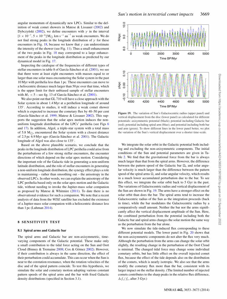
Sun’s motion in terrestrial comet impacts 3669
angular momentum of dynamically new LPCs. Similar to the def-inition of weak comet showers in Matese & Lissauer (2002) andDybczynski (2002), we define encounters with γ in the interval[1 × 10⁻⁷, 5 × 10⁻⁶] M� km s−1 au
−1as weak encounters. We do
not find strong peaks in the longitude distribution of γ for theseencounters in Fig. 18, because we know that γ can underestimatethe intensity of the shower (see Fig. 11). Thus a small enhancementof the two peaks in Fig. 18 may correspond to a large enhance-ment of the peaks in the longitude distribution as predicted by ourdynamical model in Fig. 17.
Inspecting the catalogue of the frequencies of different types ofstellar encounters in table 8 of Garcıa-Sanchez et al. (2001), we seethat there were at least eight encounters with masses equal to orlarger than one solar mass encountering the Solar system in the past10 Myr with perihelia less than 1 pc. These encounters can move toa heliocentric distance much larger than 50 pc over that time, whichis the upper limit for their unbiased sample of stellar encounterswith MV < 5 – see fig. 13 of Garcıa-Sanchez et al. (2001).
We also point out that GL 710 will have a close approach with theSolar system in about 1.4 Myr at a perihelion longitude of around135◦. According to studies, it will induce a weak comet showerwhich is expected to increase the cometary flux by 40–50 per cent(Garcıa-Sanchez et al. 1999; Matese & Lissauer 2002). This sup-ports the suggestion that the solar apex motion induces the non-uniform longitude distribution of the LPCs’ perihelia (see Figs 6and 17). In addition, Algol, a triple-star system with a total massof 5.8 M�, encountered the Solar system with a closest distanceof 2.5 pc 6.9 Myr ago (Garcıa-Sanchez et al. 2001). The Galacticlongitude of Algol was also close to 135◦.
Based on the above plausible scenario, we conclude that thepeaks in the longitude distribution of LPC perihelia could arise fromthe perturbations of a few strong stellar encounters, the encounterdirections of which depend on the solar apex motion. Consideringthe important role of the Galactic tide in generating a non-uniformlatitude distribution, and the role of stellar encounters in generatinga non-uniform longitude distribution, the synergy effect plays a rolein maintaining – rather than smoothing out – the anisotropy in theobserved LPCs. In other words, we can explain the anisotropy of theLPC perihelia based only on the solar apex motion and the Galactictide, without needing to invoke the Jupiter-mass solar companionas proposed by Matese & Whitmire (2011). To date there is noobservational evidence for such a companion. We note that a recentanalysis of data from the WISE satellite has excluded the existenceof a Jupiter-mass solar companion with a heliocentric distance lessthan 1 pc (Luhman 2014).
8 SENSITIVITY TEST
8.1 Spiral arms and Galactic bar
The spiral arms and Galactic bar are non-axisymmetric, time-varying components of the Galactic potential. These make onlya small contribution to the tidal force acting on the Sun and OortCloud (Binney & Tremaine 2008; Cox & Gomez 2002). However,if their contribution is always in the same direction, the effect oftheir perturbation could accumulate. This can occur when the Sun isnear to the corotation resonance, when the rotation velocities of thedisc and of the spiral pattern coincide. To test this hypothesis, wesimulate the solar and cometary motion adopting various constantpattern speeds of the spiral arms and the bar with fixed Galacticdensity distributions (specified in Section 3.1).
Figure 19. The variation of Sun’s Galactocentric radius (upper panel) andvertical displacement from the disc (lower panel) as calculated for differentpotentials: axisymmetric potential (black); potential including Galactic bar(red); potential including spiral arm (blue); and potential including both barand arm (green). To show different lines in the lower panel better, we plotthe variation of the Sun’s vertical displacement over a shorter time-scale.
We integrate the solar orbit in the Galactic potential both includ-ing and excluding the non-axisymmetric components. The initialconditions of the Sun and potential parameters are given in Ta-ble 2. We find that the gravitational force from the bar is alwaysmuch larger than that from the spiral arms. However, the differencebetween the pattern speed of the Galactic bar �b and solar angu-lar velocity is much larger than the difference between the patternspeed of the spiral arms �s and solar angular velocity, which resultsin a much lower accumulated perturbation due to the bar. To seethis effect, we integrate the solar orbit back to 5 Gyr in the past.The variations of Galactocentric radius and vertical displacement ofthe Sun are shown in Fig. 19. The arms have a stronger effect on thesolar orbit than does the bar. The spiral arms tend to increase theGalactocentric radius of the Sun as the integration proceeds (backin time), while the bar modulates the Galactocentric radius by acomparatively small amount. Neither the bar nor the arms signifi-cantly affect the vertical displacement amplitude of the Sun. Here,the combined perturbation from the potential including both theGalactic bar and spiral arms changes the solar motion the same wayas the perturbation from the bar alone.
We now simulate the tide-induced flux corresponding to thesedifferent potential models. The lower panel in Fig. 20 shows thatthe non-axisymmetric components do not alter the flux very much.Although the perturbation from the arms can change the solar orbitslightly, the resulting change in the perturbation of the Oort Cloudis minimal. The changed tidal force may change some individualcometary orbits, but has little effect on the overall injected cometflux, because the effect of the tide depends also on the distributionof the comets, which is nearly isotropic. We also see that the armsmodify the cometary flux more than the bar, consistent with itslarger impact on the stellar density. (The limited number of injectedcomets contributes to the sharp peaks in the relative flux difference,�fc/fc, after 3 Gyr.)
MNRAS 442, 3653–3673 (2014)
Dow
nloaded from https://academ
ic.oup.com/m
nras/article/442/4/3653/1361983 by guest on 23 September 2022

3670 F. Feng and C. A. L. Bailer-Jones
Figure 20. The magnitude of the tide-induced flux, fc, generated by theaxisymmetric potential model (upper panel) and the relative flux difference,�fc/fc, generated by asymmetric Galactic potential models (lower panel)over the past 5 Gyr with a sample of 3× 10⁴ comets. The potentials are:axisymmetric potential only (black); including the arms (blue); includingthe Galactic bar (red); including both the arms and the Galactic bar (green).
We also investigated the sensitivity of the solar motion and cometflux to the pattern speed of the asymmetric components. We findthat the closer the pattern speed of the arms is to the angular velocityof the Sun, the larger the perturbation from the arms is. (We can un-derstand this in terms of a resonance.) Meanwhile, the perturbationfrom the bar is not sensitive to the bar’s pattern speed.
Finally, we also find that the distribution of bc and lc of the cometflux does not change very much for different non-axisymmetriccomponents of the Galactic potential.
In summary, we find that the model predictions of the tide-induced cometary flux are generally insensitive to changes in thenon-axisymmetric components of the Galactic potential, exceptwhen a resonance between the arms and the solar orbit occurs,which increases the variation in the cometary flux.
8.2 Variations of the prior
As discussed earlier, the evidence depends on the prior distributionadopted for the model parameters. As this prior frequently cannotbe determined with any certainty, it is important to investigate thesensitivity of the evidence to changes in the prior.8 To completethe calculation of evidences for dynamical models, we also varythe other three initial conditions, VR(t = 0 Myr), z(t = 0 Myr), andVz(t = 0 Myr), in the EncTideSigProb models, which we previouslykept constant. Together with SigProb, EncSigProb and TideSig-Prob, this was previously the best favoured model (Table 6). Wemade numerous changes in the priors by altering their parameterranges, and re-did all necessary Monte Carlo samplings, numerical
8 A more robust – but also more time-consuming – way of calculating theevidence is presented in Bailer-Jones (2012).
simulations, and likelihood calculations and recomputed the Bayesfactors. Some of our results are shown in Table 7.
The difference in Bayes factors for random models (RandProb,RandBkgProb) and periodic models (SinProb, SinBkgProb) withdifferent prior distributions is less than five. The Bayes factors alsoremain less than 10 so they remain no better explanations of thecratering data than the Uniform model. Thus our former conclusionsabout these models are not very sensitive to plausible changes inthe priors.
The TideSigProb models in which other parameters are variedhave nearly the same evidences as the TideSigProb models listed inTable 6, so these too are insensitive to these changes in the priors.We also see that the SigProb model with positive λ has Bayes factorsmuch lower than SigProb with negative λ for both the basic150 andbasic250 data sets.
The dynamical models have parameters of the Galaxy potential,Sun’s initial conditions and combination ratio parameters (η andξ ) which are listed in Table 5. To keep things simple, we changethe fixed parameters and the ranges of the varying parameters in-dividually, and then calculate the evidence by sampling the priordefined by the changed parameter and other parameters shown inTable 5. We calculate evidences for dynamical models with doubleor half the disc mass (Md), halo mass (Mh), standard deviation ofthe initial value R (σ R), and the range of the varying ratio betweenthe EncTideProb (or TideProb) and SigProb models (η). In addition,previous studies suggest that the number of tide-induced LPCs isnot identical to the encounter-induced LPCs, i.e. ξ �= 1 (Heisler et al.1987; R08). Thus, we multiply the ratio between the tide-inducedflux and the encounter-induced flux (ξ ) by a factor of 4 or 1/4 forthe sensitivity test.
The resulting Bayes factors calculated for the basic150 data setare shown in Table 8. In each row we see little variation: the Bayesfactors are relatively insensitive to these parameters. This meansthat either the parameter space of the EncTideSigProb1 model isevenly favoured by the basic150 data set, or the data are unable todiscriminate between the compound dynamical models.
The model prediction of the anisotropic LPCs (see Fig. 17) de-pends to a greater or lesser extent on the Galactic potential, theSun’s initial condition, the Oort Cloud model, and the model ofencounters. We vary the model parameters in the same way as wedid in Table 8 and simulate ten million orbits of DLDW cometsperturbed by the tide and ten samples of stellar encounters back-wards to 10 Myr ago. We find that the latitude distribution of theLPC perihelia is not sensitive to the change of the Galactic halomass, the initial conditions of the Sun, or the direction of the so-lar apex. The amplitudes of the peaks in the latitude distributionare reduced if we decrease the mass of the Galactic disc or in-crease the stellar masses, which make the stellar encounters play amore important role in injecting comets into the loss cone. How-ever, the overall profile of the peaks is not changed in the latitudedistribution.
The peaks in the longitude distribution shift slightly if we changethe solar apex direction, the masses of the encounters, or the massof the Galactic disc. The longitude distribution is not sensitive tochanges in the other model parameters.
Finally, we also tested the effect of changing the time step in the(combined) simulations. We simulated four million comets gener-ated from the DLDW model perturbed by the tide and 10 samplesof stellar encounters backwards to 10 Myr ago using a time step of0.001 Myr (as opposed to 0.01 Myr). We find little change in eitherthe latitude or longitude distributions. In addition, we see only 4 percent more comets injected when using this smaller time step.
MNRAS 442, 3653–3673 (2014)
Dow
nloaded from https://academ
ic.oup.com/m
nras/article/442/4/3653/1361983 by guest on 23 September 2022

Sun’s motion in terrestrial comet impacts 3671
Table 7. The Bayes factors for various time series models (rows) relative to the uniform model fortwo different data sets (cf. Table 6). The second column describes what change has been made tothe range of which parameter in the prior. The other priors are kept fixed. TideSigProb3–6 refer tothe TideSigProb model in which different initial conditions are varied: VR(t = 0 Myr); z(t = 0 Myr);Vz(t = 0 Myr); and all three (respectively).
Models Varied prior Bayes factor for basic150 Bayes factor for basic250
None 4.4 3.0σ = 2σi 2.0 4.8
RandProb σ = 1/2σi 2.2 4.7N = 2Nts 1.9 1.8N = 1/2Nts 2.4 7.6
None 1.8 2.2σ = 2σi 1.6 3.7
RandBkgProb σ = 1/2σi 1.8 2.6N = 2Nts 1.5 1.5N = 1/2Nts 2.4 2.9
None 0.34 0.4310 < T < 100 0.12 0.14
SinProb2π/300 < ω < 2π/10 0.34 0.3910 < T < 300 0.88 5.4 × 10⁻²
None 1.0 1.010 < T < 100 0.90 0.88
SinBkgProb2π/300 < ω < 2π/10 1.0 1.010 < T < 300 1.8 1.4
None 15 2.0 × 10²
0 < t0 < 1.2τmax 13 1.4 × 10²SigProb −100 < λ < 100 7.7 1.0 × 10²
0 < λ < 100 1.3 × 10⁻² 1.8 × 10⁻³
None 6.4 80SinSigProb 0 < t0 < 1.2τmax 8.3 71
2π/300 < ω < 2π/10 9.9 97
TideSigProb3 None 9.0 1.7 × 10²
TideSigProb4 None 9.1 1.7 × 10²
TideSigProb5 None 9.0 1.7 × 10²
TideSigProb6 None 11 1.6 × 10²
Table 8. The Bayes factors for EncProb1, EncTideProb1 and EncTideProb1 for basic150 with different Galaxy parameters.
Models None 2Md 1/2Md 2Mh 1/2Mh 2σR 1/2σR ξ = 4 ξ = 1/4 0 < η < 8 0 < η < 2
EncProb1 1.5 2.5 3.4 2.5 4.1 2.3 2.6 – – – –EncTideProb1 1.0 2.1 2.3 2.6 3.5 1.8 1.0 1.5 0.73 – –EncTideSigProb1 11 15 11 13 12 12 11 12 10 13 8.8
In summary, we find that the overall shape of the angular distri-bution of LPC perihelia in both longitude and latitude is not verysensitive to changes in the model parameters, in particular not tothe initial distribution of Oort Cloud comets, not to the masses ofGalactic halo and disc, and not to the initial conditions of the Sun.
9 D I S C U S S I O N A N D C O N C L U S I O N
We have built dynamical models for the impact rate and angu-lar distribution of comets induced by the Galactic tide and stel-lar encounters, as modulated by the solar motion around theGalaxy. Without using the approximate methods (the averagedHamiltonian or impulse approximation), we numerically simulatethe tide-induced flux and encounter-induced flux separately. We usethese to validate the use of proxies for tide-induced flux, G3, andfor the encounter-induced flux, γ bin, in our models.
Using the Bayesian evidence framework, we find that the puretrend model (SigProb) together with the dynamical models includ-ing a trend component (EncSigProb, TideSigProb, and EncTideSig-Prob) for the cratering record are better favoured than other modelswe have tested. The trend component indicates a decreasing crater-ing rate (λ < 0) towards the past over the past 100 Myr (Gehrelset al. 1994; McEwen et al. 1997; Shoemaker 1998; Bailer-Jones2011a). This suggests that either the asteroid impact rate or thepreservation bias or both dominates the cratering record. Becausethe craters in our data sets are larger than 5 km, the preservation biasmay not be very significant over this time-scale. The disruption of asingle large asteroid could explain the trend in the data, as suggestedby Bottke et al. (2007). In addition, our models, which include thesolar apex motion, can properly predict the anisotropic perihelia ofLPCs without assuming a massive body in the outer Oort Cloud oran anisotropic Oort Cloud.
MNRAS 442, 3653–3673 (2014)
Dow
nloaded from https://academ
ic.oup.com/m
nras/article/442/4/3653/1361983 by guest on 23 September 2022

3672 F. Feng and C. A. L. Bailer-Jones
The EncTideSigProb, EncSigProb and TideSigProb models haveBayes factors of the same magnitude as the SigProb model, whichindicates that either the tide and encounter components are unnec-essary in modelling the temporal distribution of craters, or the datacannot effectively discriminate between the models.
The stochastic component in the comet flux arising from en-counters – as represented by the term γ – in the EncProb andEncTideProb models can slightly increase their evidence relative tothe TideProb model. We have performed a sensitivity test by chang-ing the prior PDF over the parameters in the dynamical models andother time series models, and find only small changes of the Bayesfactors.
The asymmetrical components in the Galactic potential could,in principle, increase the time variation of the comet flux andhence impact rate predicted by the dynamical models, by induc-ing larger deviations of the Sun’s motion from a circular orbit andthus larger changes in the local stellar density. It turns out thatthe non-axisymmetric component has relatively little impact on thepredicted cometary flux, with the exception of when the Sun is incorotation with the spiral arms. In that case the transient resonancecan produce large variations in the flux.
By including the solar apex motion, our dynamical models foranisotropic LPCs can predict reasonably well the distribution ofGalactic latitude and longitude in a set of 102 dynamically newcomets. In this model, the asymmetry in the distribution of Galacticlatitudes caused by the Sun’s current location and its motion over thepast 10 Myr (comparable with the time-scale of a comet shower).
The two narrow peaks in the cometary perihelia at lc = 135◦
and 315◦ could be caused by a handful of strong stellar encountersencountering the Sun with their encountering velocities in the di-rection of antapex in the HRF. On the other hand, we might alsosee something similar due to the periodic orbital motion about theSun of a massive body (such as a brown dwarf) residing within theOort Cloud (Matese et al. 1999; Matese & Whitmire 2011). How-ever, our dynamical model, which takes into account the solar apexmotion, can predict the longitudinal asymmetry without assumingthe existence of such a body. In addition, the latitude distribution ofLPC perihelia predicted by our simulations is consistent with thetheoretical prediction, although one peak in the observed distribu-tion is not properly predicted by our simulations. The synergy effectbetween the encounters and the tide cannot entirely eliminate theanisotropy induced by either the tide or the encounters.
A non-uniform distribution in the perihelion direction of en-counters was found by Garcıa-Sanchez et al. (2001), although thesignal is of questionable significance due to the incompleteness, i.e.faint stars which high velocities being too faint after 10 Myr forHipparcos to have observed.
An anisotropy in the longitude of LPCs will not correspond toan anisotropy in longitudes of impacts on the Earth’s surface due tothe rotation of the Earth and its orbit about the Sun. Some latitudevariation may be expected, despite the long-term variation in incli-nation and obliquity of the Earth’s orbit (Le Feuvre & Wieczorek2008; Werner & Medvedev 2010). Disrupted comets generally re-tain their original orbital plane (Bottke et al. 2002), so the resultingasteroids would tend to impact in the plane perpendicular to solarapex. Yet these are all higher order effects which would be difficultto convincingly detect and relate to the solar orbit in the analysis ofterrestrial impact craters.
Our modelling approach has, like any other, introduced variousassumptions and approximations. We have ignored the synergy ef-fect between the Galactic tide and stellar encounters highlighted byR08. We instead simply sum the tide-induced flux and the encounter-
induced flux in the ratio ξ to 1. Because the cometary impact ratemodulated by the solar motion around the Galactic centre seemsto be unnecessary in order to explain the data, the synergy effect,which is also influenced by the solar motion, may not change theresult significantly. In addition, we use a decreasing impact rate to-wards the past (negative trend component) to model the combinedeffect of preservation bias and asteroid impact rate. In modelling theangular distribution of the LPC perihelia, the sample noise in thecomets injected into the observable zone prevent us from buildinga more robust model, especially for the longitude distribution. Thisproblem could be resolved by calculating perturbations based on amore accurately measured Galactic tide and using an actual cata-logue of encountering stars in the solar neighbourhood as opposedto our stochastic model of plausible encounters.
In common with some other studies (e.g. R08; Wickramasinghe& Napier 2008; Fouchard et al. 2011; Gardner et al. 2011), wehave ignored the perturbing effect on comets from the giant planets,although we acknowledge that the giants planets could influence thepredicted LPC flux in particular (Kaib & Quinn 2009). The planetaryperturbations can also change the fraction of the inner Oort Cloudcomets among the injected LPCs (Kaib & Quinn 2009), which inturn could change the angular distribution of the LPC perihelia.However, these perturbations should not have a significant effectover the relatively short time-scale of 10 Myr which we use in thesimulations to generate the LPC distribution. As the main goal ofour work is to study the variable effect of the solar orbit on the LPCflux and angular distribution, rather than to predict the absoluteLPC flux precisely, our conclusions should not be overly affectedby neglecting the giant planets in this way.
In the future, the Gaia survey allow us to detect many more re-cent stellar encounters down to fainter magnitude limits and largerdistances than Hipparcos, thereby allowing us to extend the time-scale over which we can get a complete sample of recent stellarencounters. The Gaia magnitude limit of G = 20 which is lowenough to cover the high velocity stars in a time-scale of 10 Myr.For example, a star with absolute magnitude of 10 and a velocityof 80 km s−1 in the HRF would move 800 pc in 10 Myr and so havean apparent magnitude of 19.5. Thus, Gaia will be able to observeall stars more massive than early M dwarfs (and thus essentially allrelevant stars) encountering the Solar system over the past 10 Myr.For more recent time-scales Gaia can observe even less massiveobjects. Moreover, the Gaia catalogue of more massive stellar en-counters (stars with absolute magnitudes larger than that of theSun) may shed light on the study of terrestrial craters over sincethe beginning of the Phanerozoic era, some 550 Myr ago. Gaia canfurther improve the measurement of Sun’s initial conditions andthe potential of the Galaxy (Lindegren et al. 2008; Koposov, Rix& Hogg 2010). After including planetary perturbations, this wouldmake the simulation of cometary orbits accurate enough to trace thestellar encounter back to the time when it generated comet showersand corresponding terrestrial craters (Rickman et al. 2012).
AC K N OW L E D G E M E N T S
We thank Carmen Martinez, Inti Pelupessy, and Arjen van Elterenfor explaining, installing, and testing the AMUSE framework. We areindebted to Anthony Brown and Piotr A. Dybczynski for their use-ful suggestions. We are grateful to the referee, Nathan Kaib, forconstructive comments which helped to improve the manuscript.This work has been carried out as part of the Gaia Research forEuropean Astronomy Training (GREAT-ITN) network. The re-search leading to these results has received funding from the
MNRAS 442, 3653–3673 (2014)
Dow
nloaded from https://academ
ic.oup.com/m
nras/article/442/4/3653/1361983 by guest on 23 September 2022

Sun’s motion in terrestrial comet impacts 3673
European Union Seventh Framework Programme ([FP7/2007-2013] under grant agreement no. 264895.
R E F E R E N C E S
Alvarez W., Muller R. A., 1984, Nature, 308, 718Alvarez L. W., Alvarez W., Asaro F., Michel H. V., 1980, Science, 208, 1095Bailer-Jones C. A. L., 2009, Int. J. Astrobiol., 8, 213Bailer-Jones C. A. L., 2011a, MNRAS, 416, 1163Bailer-Jones C. A. L., 2011b, MNRAS, 418, 2111Bailer-Jones C. A. L., 2012, A&A, 546, A89Bate R. R., Mueller D. D., White J. E., 1971, Fundamentals of Astrodynam-
ics. Dover Press, New YorkBiermann L., Huebner W. F., Lust R., 1983, Proc. Natl. Acad. Sci., 80, 5151Binney J., Tremaine S., 2008, Galactic Dynamics, 2nd edn. Princeton Univ.
Press, Princeton, NJBogart R. S., Noerdlinger P. D., 1982, AJ, 87, 911Bottke W. F., Morbidelli A., Jedicke R., Petit J.-M., Levison H. F., Michel
P., Metcalfe T. S., 2002, Icarus, 156, 399Bottke W. F., David V., David N., 2007, Nature, 449, 48Brasser R., Higuchi A., Kaib N., 2010, A&A, 516, A72Cox D. P., Gomez G. C., 2002, ApJS, 142, 261Dehnen W., 2000, AJ, 119, 800Dehnen W., Binney J. J., 1998, MNRAS, 298, 387Delsemme A. H., 1987, A&A, 187, 913Dones L., Weissman P. R., Levison H. F., Duncan M. J., 2004a, in Johnstone
D., Adams F. C., Lin D. N. C., Neufeeld D. A., Ostriker E. C., eds, ASPConf. Ser. Vol. 323, Star Formation in the Interstellar Medium: In Honorof David Hollenbach. Astron. Soc. Pac., San Francisco, p. 371
Dones L., Weissman P. R., Levison H. F., Duncan M. J., 2004b,Oort Cloud Formation and Dynamics. Comets II, 153, available at:http://www.lpi.usra.edu/books/CometsII/7031.pdf
Drimmel R., 2000, A&A, 358, L13Duncan M., Quinn T., Tremaine S., 1987, AJ, 94, 1330Dybczynski P. A., 2002, A&A, 396, 283Dybczynski P. A., 2005, A&A, 441, 783Earth Impact Database 2011, available at: http://www.unb.ca/passc/
ImpactDatabase/, Accessed 1 May 2013Emel’yanenko V. V., Asher D. J., Bailey M. E., 2007, MNRAS, 381, 779Feng F., Bailer-Jones C. A. L., 2013, ApJ, 768, 152Fouchard M., 2004, MNRAS, 349, 347Fouchard M., Froeschle C., Rickman H., Valsecchi G. B., 2011, Icarus, 214,
334Francis P. J., 2005, ApJ, 635, 1348Fujii M., Iwasawa M., Funato Y., Makino J., 2007, PASJ, 59, 1095Garcıa-Sanchez J., Preston R. A., Jones D. L., Weissman P. R., Lestrade
J.-F., Latham D. W., Stefanik R. P., 1999, AJ, 117, 1042Garcıa-Sanchez J., Weissman P. R., Preston R. A., Jones D. L., Lestrade
J.-F., Latham D. W., Stefanik R. P., Paredes J. M., 2001, A&A, 379, 634Gardner E., Nurmi P., Flynn C., Mikkola S., 2011, MNRAS, 411, 947Gehrels T., Matthews M. S., Schumann A. M., eds, 1994, Hazards due to
Comets and Asteroids. Univ. Arizona Press, Tucson, p. 897Grieve R. A. F., Pesonen L. J., 1996, Earth Moon and Planets, 72, 357Heisler J., Tremaine S., Alcock C., 1987, Icarus, 70, 269Hildebrand A. R., Penfield G. T., Kring D. A., Pilkington M., Camargo
Z. A., Jacobsen S. B., Boynton W. V., 1991, Geology, 19, 867Hills J. G., 1981, AJ, 86, 1730
Jetsu L., Pelt J., 2000, A&A, 353, 409Kaib N. A., Quinn T., 2009, Science, 325, 1234Kaib N. A., Quinn T., Brasser R., 2011a, ApJ, 141, 3Kaib N. A., Roskar R., Quinn T., 2011b, Icarus, 215, 491Kass R. E., Raftery A. E., 1995, J. Am. Stat. Assoc., 90, 773Khanna M., Sharma S. D., 1983, PASJ, 35, 559Koposov S. E., Rix H.-W., Hogg D. W., 2010, ApJ, 712, 260Le Feuvre M., Wieczorek M. A., 2008, Icarus, 197, 291Levison H. F., Duncan M. J., Brasser R., Kaufmann D. E., 2010, Science,
329, 187Lindegren L. et al., 2008, in Jin W. J., Platais I., Perryman M. A. C., eds, IAU
Symp. 248, A Giant Step: from Milli- to Micro-arcsecond Astrometry.Cambridge Univ. Press, Cambridge, p. 217
Luhman K. L., 2014, ApJ, 781, 4McEwen A. S., Moore J. M., Shoemaker E. M., 1997, J. Geophys. Res.,
102, 9231Majaess D. J., Turner D. G., Lane D. J., 2009, MNRAS, 398, 263Marsden B. G., Williams G. V., 2008, Catalogue of Cometary Orbits, 17th
edn. Smithsonian Astrophysical Observatory, Cambridge, MAMartos M., Yanez M., Hernandez X., Moreno E., Pichardo B., 2004, J.
Korean Astron. Soc., 37, 199Matese J. J., Lissauer J. J., 2002, Icarus, 157, 228Matese J. J., Whitmire D. P., 2011, Icarus, 211, 926Matese J. J., Whitman P. G., Whitmire D. P., 1999, Icarus, 141, 354Melott A. L., Bambach R. K., 2011, Paleobiology, 37, 383Oort J. H., 1950, Bull. Astron. Inst. Netherlands, 11, 91Pelupessy F. I., Janes J., Portegies Zwart S., 2012, New Astron., 17, 711Pelupessy F. I., van Elteren A., de Vries N., McMillan S. L. W., Drost N.,
Portegies Zwart S. F., 2013, A&A, 557, A84Portegies Zwart S., McMillan S. L. W., van Elteren E., Pelupessy I., de Vries
N., 2013, Comput. Phys. Commun., 183, 456Raup D. M., Sepkoski J. J., 1984, Proc. Natl. Acad. Sci., 81, 801Rickman H., 1976, Bull. Astron. Inst. Czech., 27, 92Rickman H., Fouchard M., Valsecchi G. B., Froeschle C., 2005, Earth Moon
Planets, 97, 411Rickman H., Fouchard M., Froeschle C., Valsecchi G. B., 2008, Celest.
Mech. Dyn. Astron., 102, 111 (R08)Rickman H., Fouchard M., Froeschle C., Valsecchi G. B., 2012, Planet.
Space Sci., 73, 124Rohde R. A., Muller R. A., 2005, Nature, 434, 208Schonrich R., 2012, MNRAS, 427, 274Schonrich R., Binney J., Dehnen W., 2010, MNRAS, 403, 1829Shoemaker E. M., 1998, J. R. Astron. Soc. Can., 92, 297Wainscoat R. J., Cohen M., Volk K., Walker H. J., Schwartz D. E., 1992,
ApJS, 83, 111Weissman P. R., 2007, in Valsecchi G. B., Vokrouhlicky D., Milani A., eds,
IAU Symp. 236, Near Earth Objects, our Celestial Neighbors: Opportu-nity and Risk. Cambridge Univ. Press, Cambridge, p. 441
Werner S. C., Medvedev S., 2010, Earth Planet. Sci. Lett., 295, 147Wickramasinghe J. T., Napier W. M., 2008, MNRAS, 387, 153Wiegert P., Tremaine S., 1999, Icarus, 137, 84Wisdom J., Holman M., 1991, AJ, 102, 1528Yabushita S., 1996, MNRAS, 279, 727
This paper has been typeset from a TEX/LATEX file prepared by the author.
MNRAS 442, 3653–3673 (2014)
Dow
nloaded from https://academ
ic.oup.com/m
nras/article/442/4/3653/1361983 by guest on 23 September 2022