Exploring optimal design of look-up table for PROSAIL model inversion with multi-angle MODIS data

Exploring optimal design of look-up table for PROSAIL model

inversion with multi-angle MODIS data

Wei He∗, Hua Yang, Jingjing Pan, Peipei Xu

School of Geography and Remote Sensing Science, Beijing Normal University; Beijing Key

Laboratory of Environmental Remote Sensing and Digital City; State Key Laboratory of Remote

Sensing Science, Jointly Sponsored by Beijing Normal University and the Institute of Remote Sensing

Applications, CAS; Beijing, China 100875

ABSTRACT

Physical remote sensing model inversion based on look-up table (LUT) technique is promising for its good precision,

high efficiency and easily-realization. However, scheme of the LUT is difficult to be well designed, as lacking a thorough

investigation of its mechanism for different designs, for instance, the way the parameter space is sampled. To studying this

problem, experiments on several LUT design schemes are performed and their effects on inversion results are analyzed in

this paper. 1,000 groups of randomly generated parameters of PROSAIL model are taken to simulate multi-angle

observations with the observation angles of MODIS sensor to be inversion data. The correlation coefficient (R2) and root

mean square error (RMSE) of input LAIs for simulation and estimated LAIs were calculated. The results show that, LUT

size is a key factor, and the RMSE is lower than 0.25 when the size reaches 100,000; Selecting no more than 0.1% cases of

the LUT as the solution with a size of 100,000 is usually valid and the RMSE is usually increased with the increasing of the

percentage of selected cases; Taking the median of the selected solutions as the final solution is better than the mean or the

“best” whose cost function value is the least; Different parameter distributions have a certain impact on the inversion

results, and the results get better when using a normal distribution. Finally, winter wheat LAI of one research area in

Xinxiang City, Henan Province of China is estimated with MODIS daily reflectance data, the validate result shows it

works well.

Keywords: look-up table, leaf area index, PROSAIL model, MODIS, winter wheat

1. INTRODUCTION

Leaf Area Index (LAI), defined as one half of the total green leaf area per unit horizontal ground surface area, is a key

structural parameter of vegetation because of the role of green leaves in controlling many biological and physical processes

of plant canopies. It is also an important input into models quantifying the exchange of energy and matter between the land

surface and the atmosphere.

∗ Email:[email protected]; Tel: (+86) 01058807454-1450; Fax: (+86) 01058809977.

Land Surface Remote Sensing, edited by Dara Entekhabi, Yoshiaki Honda, Haruo Sawada, Jiancheng Shi, Taikan Oki, Proc. of SPIE Vol. 8524, 852420 · © 2012 SPIE · CCC code: 0277-786/12/$18 · doi: 10.1117/12.977234

Proc. of SPIE Vol. 8524 852420-1

Downloaded From: http://proceedings.spiedigitallibrary.org/ on 04/23/2013 Terms of Use: http://spiedl.org/terms

The common methods to estimate LAI include empirical formula, networks and look-up tables. But all of them have

some limitations, and LUT has several advantages. Perhaps the simplest inversion method of a radiative transfer model is

using a LUT. LUTs offer an interesting alternative to numerical optimization and neural network methods because they

permit a global search (avoid local minima) while showing less unexpected behavior when the spectral characteristics of

the targets are not well represented by the modeled spectra [1].

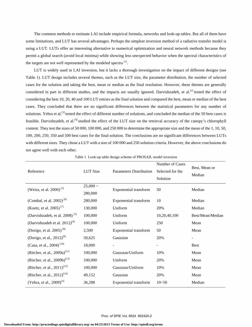
LUT is widely used in LAI inversion, but it lacks a thorough investigation on the impact of different designs (see

Table 1). LUT design includes several themes, such as the LUT size, the parameter distribution, the number of selected

cases for the solution and taking the best, mean or median as the final resolution. However, these themes are generally

considered in part in different studies, and the impacts are usually ignored. Darvishzadeh, et al.[2] tested the effect of

considering the best 10, 20, 40 and 100 LUT entries as the final solution and compared the best, mean or median of the best

cases. They concluded that there are no significant differences between the statistical parameters for any number of

solutions. Yebra et al.[3] tested the effect of different number of solutions, and concluded the median of the 50 best cases is

feasible. Darvishzadeh, et al.[4] studied the effect of the LUT size on the retrieval accuracy of the canopy’s chlorophyll

content. They test the sizes of 50 000, 100 000, and 250 000 to determine the appropriate size and the mean of the 1, 10, 50,

100, 200, 250, 350 and 500 best cases for the final solution. The conclusions are no significant differences between LUTs

with different sizes. They chose a LUT with a size of 100 000 and 250 solution criteria. However, the above conclusions do

not agree well with each other.

Table 1 Look-up table design scheme of PROSAIL model inversion

Reference LUT Size Parameters Distribution

Number of Cases

Selected for the

Solution

Best, Mean or

Median

(Weiss, et al. 2000) [5] 25,000 ~

280,000 Exponential transform 50 Median

(Combal, et al. 2002) [6] 280,000 Exponential transform 10 Median

(Koetz, et al. 2005) [7] 130,000 Uniform 20% Median

(Darvishzadeh, et al. 2008) [2] 100,000 Uniform 10,20,40,100 Best/Mean/Median

(Darvishzadeh et al. 2012)[4] 100,000 Uniform 250 Mean

(Dorigo, et al. 2005) [8] 2,500 Exponential transform 50 Mean

(Dorigo, et al., 2012)[9] 50,625 Gaussian 20% -

(Casa, et al., 2004) [10] 18,000 - - Best

(Ritcher, et al., 2009a)[11] 100,000 Gaussian/Uniform 10% Mean

(Ritcher, et al., 2009b)[12] 100,000 Uniform 20% Mean

(Ritcher, et al., 2011)[13] 100,000 Gaussian/Uniform 10% Mean

(Ritcher, et al., 2012)[14] 49,152 Gaussian 20% Mean

(Yebra, et al., 2009)[3] 36,288 Exponential transform 10~50 Median



Therefore, the main objective of this study is to systematically investigate the impact of different designs on model

inversion, thus attempts to explore an optimal design of look-up table for PROSAIL model inversion with multi-angle

remote sensing data. In this paper, the impact of different factors of LUT design, such as the size of the LUT, the number

of the best cases, the mean or median of the best cases, was investigated. Then it was applied to winter wheat LAI inversion

and the precision of this algorithm was validated.

2. METHODOLOGY

2.1 Radiative transfer model and inversion procedures

The widely used PROSAIL radiative transfer model [15], which is a combination of the SAIL canopy reflectance

model [16, 17] and the PROSPECT leaf optical properties model [18], was used in this study. The SAIL model is a one

dimensional turbid medium radiative transfer model that describes the canopy as infinitely horizontally extended layers

where leaves are randomly distributed. The present study used a modified version of the SAIL model that was adapted to

account for the hotspot effect [19]. Canopy structure is characterized by LAI, the average leaf angle inclination (ALA) and

the hot-spot parameter (H). The leaf hemispherical reflectance (LR) and transmittance (LT) which required as SAIL model

input parameters are supplied by the PROSPECT model as a function of the mesophyll structure parameter (N),

chlorophyll (Cab), dry matter (Cm), relative water (Cw) and brown pigment (Cbp) contents. Reflectance of soils was

simulated using five typical soil reflectance spectra multiplied by a brightness coefficient Psoil. It allows representing with

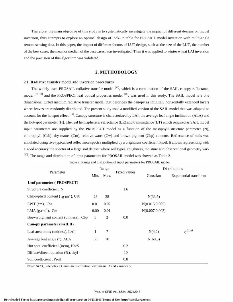
a good accuracy the spectra of a large soil dataset where soil types, roughness, moisture and observational geometry vary [20]. The range and distribution of input parameters for PROSAIL model was showed as Table 2.

Table 2 Range and distribution of input parameters for PROSAIL model

Parameter Range

Fixed values Distributions

Min. Max. Gaussian Exponential transform

Leaf parameter ( PROSPECT)

Structure coefficient, N 1.6

Chlorophyll content ( 2μg cm−⋅ ), Cab 28 38 N(33,5)

EWT (cm), Cw 0.01 0.02 N(0.015,0.005)

LMA (g.cm-2), Cm 0.00 0.01 N(0.007,0.003)

Brown pigment content (unitless), Cbp 3 2 0.0

Canopy parameter (SAILH)

Leaf area index (unitless), LAI 1 7 N(4,2) -2LAIe

Average leaf angle (°), ALA 50 70 N(60,5)

Hot spot coefficient (m/m), HotS 0.2

Diffuse/direct radiation (%), skyl 10

Soil coefficient , Psoil 0.8

Note: N(33,5) denotes a Gaussian distribution with mean 33 and variance 5.



For estimating the parameters of the PROSAIL model, an adequate inversion procedure has to be defined. For this

purpose, a look-up table approach was chosen as the inversion approach. 100,000 or more simulations of PROSAIL model

were generated. For the LUT, a simple cost function composed of the root mean square error (RMSE) was employed.

Hereby, the spectra of the closest (radiometric) match with the measured signal were selected.

2.2 Experiment design

In order to investigate the impact of look-up table design schemes on model inversion, a synthetic observation data

base with a size of 1,000 was generated using PROSAIL model. PROSAIL was configured for the simulation of MODIS

sensors spectral band configurations according to the sensor spectral response functions. In this study, just LAI is taken as

the retrieval parameter for example, and the root mean square error (RMSE) between the input LAIs for simulation and the

estimated LAIs were calculated to evaluate the best design scheme.

The size of the LUT, different parameter distributions, and the way the solution is extracted from the table such as the

best, mean or median of the 50 or more cases were tested. Because the sampling is not of equal interval and they have

certain randomness, every generation was repeated for 2 times.

3．RESULTS AND DISCUSSION

3.1 Effect of the LUT size

For the inversion, only search operations are needed to identify the parameter combinations that yield the best fit

between measured and LUT spectra. However, to attain high accuracy for the estimated parameters, the dimension of the

LUT must be sufficiently large [5, 6].

If the size of the table is small, tables generated at different times would be of great difference, and the inversion is

dependent on the table generated at one time. Only when the size is great enough, stable inversion results can be achieved.

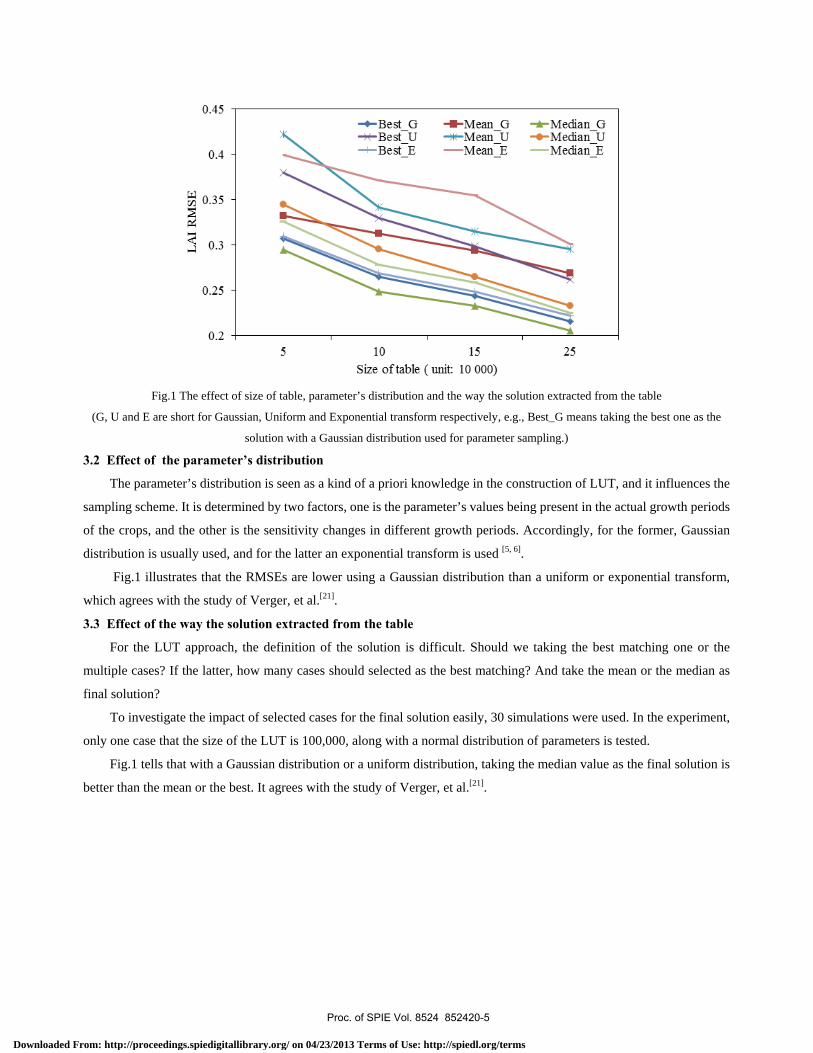
Fig.1 shows that greater the size of the table is, more precise the inversion result is. However, when the size of LUT

reaches a certain point, the improvement is faint and the efficiency may decline sharply. So the optimal scheme is a

compromise of precision and efficiency.

The size needs to be determined by experiments when we apply a LUT approach for model inversion. The size may

due to number of the inverted parameters and their uncertain ranges.



5 10 15

Size of table (unit 10 000)

Fig.1 The effect of size of table, parameter’s distribution and the way the solution extracted from the table

(G, U and E are short for Gaussian, Uniform and Exponential transform respectively, e.g., Best_G means taking the best one as the

solution with a Gaussian distribution used for parameter sampling.)

3.2 Effect of the parameter’s distribution

The parameter’s distribution is seen as a kind of a priori knowledge in the construction of LUT, and it influences the

sampling scheme. It is determined by two factors, one is the parameter’s values being present in the actual growth periods

of the crops, and the other is the sensitivity changes in different growth periods. Accordingly, for the former, Gaussian

distribution is usually used, and for the latter an exponential transform is used [5, 6].

Fig.1 illustrates that the RMSEs are lower using a Gaussian distribution than a uniform or exponential transform,

which agrees with the study of Verger, et al.[21].

3.3 Effect of the way the solution extracted from the table

For the LUT approach, the definition of the solution is difficult. Should we taking the best matching one or the

multiple cases? If the latter, how many cases should selected as the best matching? And take the mean or the median as

final solution?

To investigate the impact of selected cases for the final solution easily, 30 simulations were used. In the experiment,

only one case that the size of the LUT is 100,000, along with a normal distribution of parameters is tested.

Fig.1 tells that with a Gaussian distribution or a uniform distribution, taking the median value as the final solution is

better than the mean or the best. It agrees with the study of Verger, et al.[21].



0.5

0.45

0.4

0.35

0.3

0.25

.4 0.2

0.15

0.1

0.05

0. N CI) v-1 r-- CI N R 10 CO O N I' 0 COÓ Ó Ó Ó Ó Ó

Percentage of selected cases ( %)

N

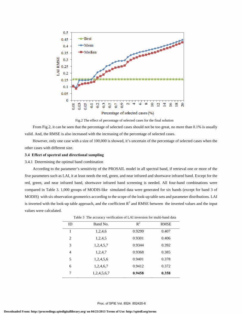
Fig.2 The effect of percentage of selected cases for the final solution

From Fig.2, it can be seen that the percentage of selected cases should not be too great, no more than 0.1% is usually

valid. And, the RMSE is also increased with the increasing of the percentage of selected cases.

However, only one case with a size of 100,000 is showed, it’s uncertain of the percentage of selected cases when the

other cases with different size.

3.4 Effect of spectral and directional sampling

3.4.1 Determining the optimal band combination

According to the parameter’s sensitivity of the PROSAIL model in all spectral band, if retrieval one or more of the

five parameters such as LAI, it at least needs the red, green, and near infrared and shortwave infrared band. Except for the

red, green, and near infrared band, shortwave infrared band screening is needed. All four-band combinations were

compared in Table 3. 1,000 groups of MODIS-like simulated data were generated for six bands (except for band 3 of

MODIS) with six observation geometrics according to the scope of the look-up table sets and parameter distributions. LAI

is inverted with the look-up table approach, and the coefficient R2 and RMSE between the inverted values and the input

values were calculated.

Table 3 The accuracy verification of LAI inversion for multi-band data

ID Band No. R2 RMSE

1 1,2,4,6 0.9299 0.407

2 1,2,4,5 0.9301 0.406

3 1,2,4,5,7 0.9344 0.392

4 1,2,4,7 0.9368 0.385

5 1,2,4,5,6 0.9401 0.378

6 1,2,4,6,7 0.9412 0.372

7 1,2,4,5,6,7 0.9458 0.358



á8

(a)

2 3 4 5True LAI

(d)

6 7

8

8

7

6

5

i. 3 angles-fitting line

(e)

(f)

The R2 of the group 7 is the greatest and its RMSE is the lowest (see Table 3), so this combination is the best band

combination.

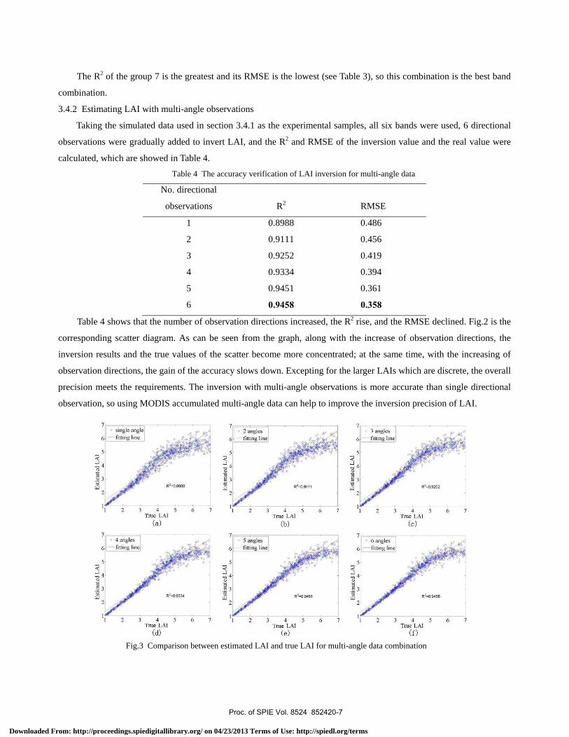
3.4.2 Estimating LAI with multi-angle observations

Taking the simulated data used in section 3.4.1 as the experimental samples, all six bands were used, 6 directional

observations were gradually added to invert LAI, and the R2 and RMSE of the inversion value and the real value were

calculated, which are showed in Table 4.

Table 4 The accuracy verification of LAI inversion for multi-angle data

No. directional

observations

R2

RMSE

1 0.8988 0.486

2 0.9111 0.456

3 0.9252 0.419

4 0.9334 0.394

5 0.9451 0.361

6 0.9458 0.358

Table 4 shows that the number of observation directions increased, the R2 rise, and the RMSE declined. Fig.2 is the

corresponding scatter diagram. As can be seen from the graph, along with the increase of observation directions, the

inversion results and the true values of the scatter become more concentrated; at the same time, with the increasing of

observation directions, the gain of the accuracy slows down. Excepting for the larger LAIs which are discrete, the overall

precision meets the requirements. The inversion with multi-angle observations is more accurate than single directional

observation, so using MODIS accumulated multi-angle data can help to improve the inversion precision of LAI.

Fig.3 Comparison between estimated LAI and true LAI for multi-angle data combination



36° 0'0 "N

35° 0'0 "N

34° 0'0 "N

33° 0' 0 "N

32° 0' 0 "N

31° 0'0 "N

3.5 Case study: Winter wheat LAI inversion with MODIS daily reflectance

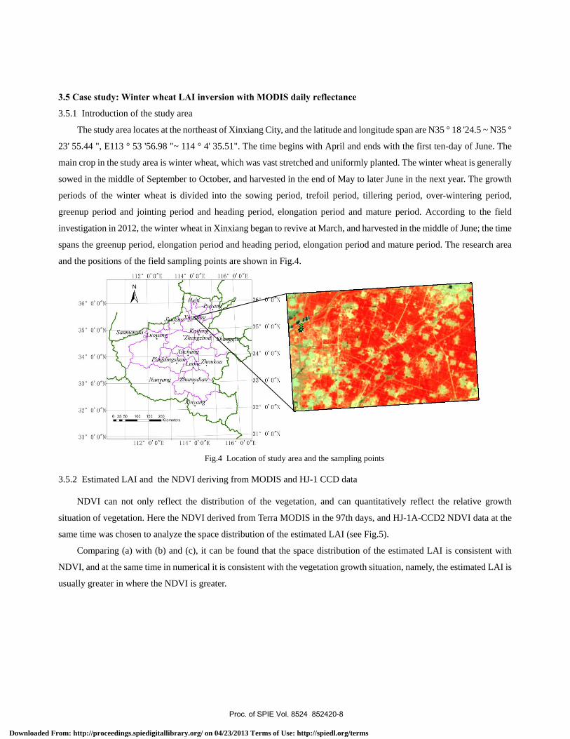
3.5.1 Introduction of the study area

The study area locates at the northeast of Xinxiang City, and the latitude and longitude span are N35 ° 18 '24.5 ~ N35 °

23' 55.44 ", E113 ° 53 '56.98 "~ 114 ° 4' 35.51". The time begins with April and ends with the first ten-day of June. The

main crop in the study area is winter wheat, which was vast stretched and uniformly planted. The winter wheat is generally

sowed in the middle of September to October, and harvested in the end of May to later June in the next year. The growth

periods of the winter wheat is divided into the sowing period, trefoil period, tillering period, over-wintering period,

greenup period and jointing period and heading period, elongation period and mature period. According to the field

investigation in 2012, the winter wheat in Xinxiang began to revive at March, and harvested in the middle of June; the time

spans the greenup period, elongation period and heading period, elongation period and mature period. The research area

and the positions of the field sampling points are shown in Fig.4.

Fig.4 Location of study area and the sampling points

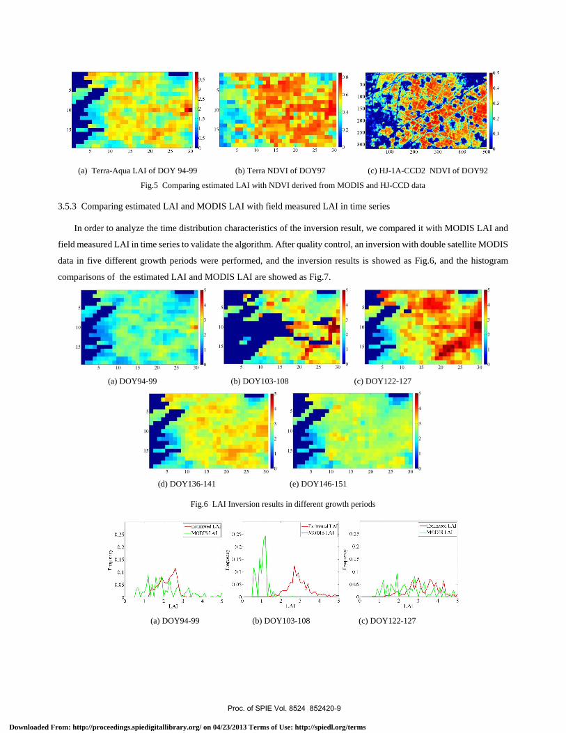
3.5.2 Estimated LAI and the NDVI deriving from MODIS and HJ-1 CCD data

NDVI can not only reflect the distribution of the vegetation, and can quantitatively reflect the relative growth

situation of vegetation. Here the NDVI derived from Terra MODIS in the 97th days, and HJ-1A-CCD2 NDVI data at the

same time was chosen to analyze the space distribution of the estimated LAI (see Fig.5).

Comparing (a) with (b) and (c), it can be found that the space distribution of the estimated LAI is consistent with

NDVI, and at the same time in numerical it is consistent with the vegetation growth situation, namely, the estimated LAI is

usually greater in where the NDVI is greater.



5

10

15

5 10 15 20 25 30

3.5

3

2.5

2

1.5

1

0.5

0

1

1

100 200 300 400 500

0.5

0.4

0.3

1.2

0.1

0

5

0 15 20 250

u

15 211 25 îil o

10 Fr15

5 10 15 20 25 30

+3

0.25

0.2UL".

0.15

0.1

0.05

0

- Estimated LAI-MODIS LAI

LAI

0.25 -

0.2 -UL"r

0.15-.w

0.1

0.05 -


2 3LAI

4 5

0.25 -

0.2 -

0.1

- Estimated LAI

-MODIS LAI

LAI

(a) Terra-Aqua LAI of DOY 94-99 (b) Terra NDVI of DOY97 (c) HJ-1A-CCD2 NDVI of DOY92

Fig.5 Comparing estimated LAI with NDVI derived from MODIS and HJ-CCD data

3.5.3 Comparing estimated LAI and MODIS LAI with field measured LAI in time series

In order to analyze the time distribution characteristics of the inversion result, we compared it with MODIS LAI and

field measured LAI in time series to validate the algorithm. After quality control, an inversion with double satellite MODIS

data in five different growth periods were performed, and the inversion results is showed as Fig.6, and the histogram

comparisons of the estimated LAI and MODIS LAI are showed as Fig.7.

(a) DOY94-99 (b) DOY103-108 (c) DOY122-127

(d) DOY136-141 (e) DOY146-151

Fig.6 LAI Inversion results in different growth periods

(a) DOY94-99 (b) DOY103-108 (c) DOY122-127



0.25 -

0.2 -UL".

, 0.15 -.w

0.1

0.05 -

00


2 3LM

5

0.25

0.2UL"., 0.15

0.1

0.05


0 1 2 3LAI

5

5.5

4.5

z 3.5

^ o

2.5

1.5

0.5D0Y94 DOY103 D0Y122 D0Y136 D0Y146

Time

5.5

4.5

3.5at

3

2.5

1.5

0.5

Pixel 1

Pixel 2

-e- Pixel 3

-3- Pixel 4Field LAI

D0Y97 DOY105 DOY121 D0Y137 DOY145

Time

(d) DOY136-141 (e) DOY146-151

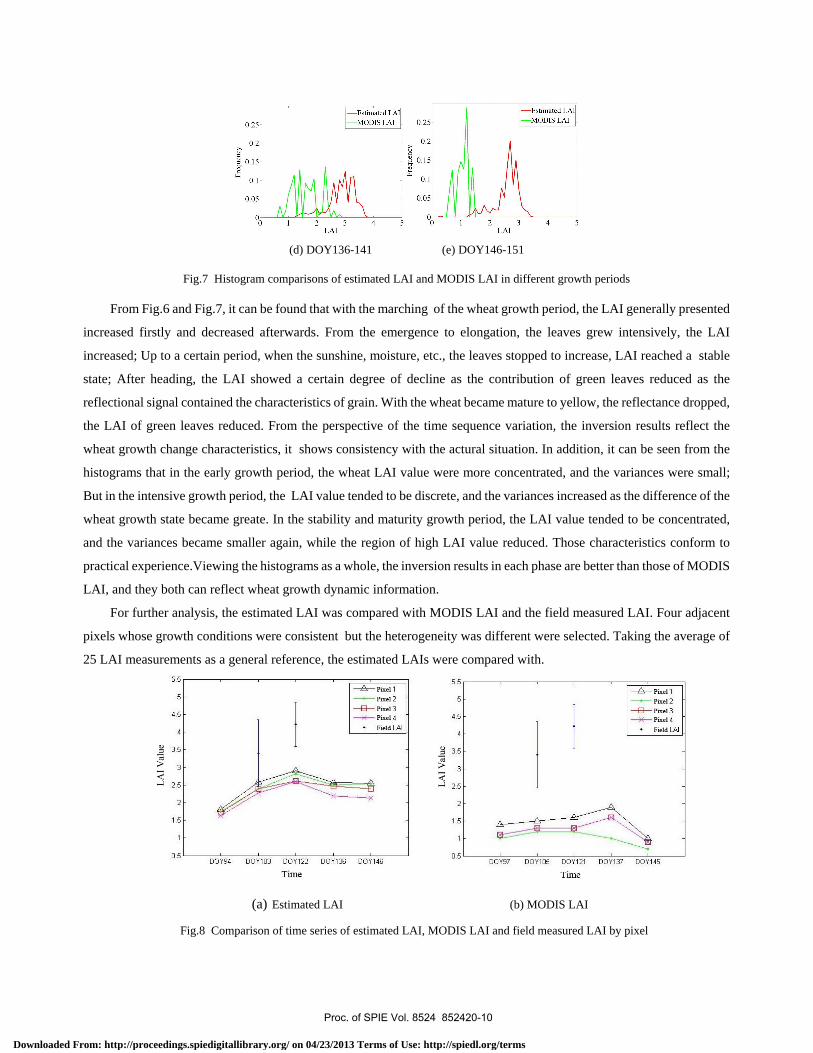
Fig.7 Histogram comparisons of estimated LAI and MODIS LAI in different growth periods

From Fig.6 and Fig.7, it can be found that with the marching of the wheat growth period, the LAI generally presented

increased firstly and decreased afterwards. From the emergence to elongation, the leaves grew intensively, the LAI

increased; Up to a certain period, when the sunshine, moisture, etc., the leaves stopped to increase, LAI reached a stable

state; After heading, the LAI showed a certain degree of decline as the contribution of green leaves reduced as the

reflectional signal contained the characteristics of grain. With the wheat became mature to yellow, the reflectance dropped,

the LAI of green leaves reduced. From the perspective of the time sequence variation, the inversion results reflect the

wheat growth change characteristics, it shows consistency with the actural situation. In addition, it can be seen from the

histograms that in the early growth period, the wheat LAI value were more concentrated, and the variances were small;

But in the intensive growth period, the LAI value tended to be discrete, and the variances increased as the difference of the

wheat growth state became greate. In the stability and maturity growth period, the LAI value tended to be concentrated,

and the variances became smaller again, while the region of high LAI value reduced. Those characteristics conform to

practical experience.Viewing the histograms as a whole, the inversion results in each phase are better than those of MODIS

LAI, and they both can reflect wheat growth dynamic information.

For further analysis, the estimated LAI was compared with MODIS LAI and the field measured LAI. Four adjacent

pixels whose growth conditions were consistent but the heterogeneity was different were selected. Taking the average of

25 LAI measurements as a general reference, the estimated LAIs were compared with.

(a) Estimated LAI (b) MODIS LAI

Fig.8 Comparison of time series of estimated LAI, MODIS LAI and field measured LAI by pixel

Proc. of SPIE Vol. 8524 852420-10


Fig.8 shows this inversion results and MODIS LAI are smaller than the field measured values, but this inversion

results are more close to the measured. For both this algorithm and the MODIS algorithm, the inversion results are smaller

than the field measured, which may be due to the influence of the mixed pixels. The plants in the measured districts grew

well, and "pure" block whose soil background interference was weak, but the 500 square meters region of a MODIS pixel

was likely highly-mixed. The study of Yang, et al.[22] and Bai, et al.[23] demonstrated that the estimated LAI using the

MODIS data was significantly less than that of TM data. For a same land surface, the estimated LAI values in pure pixels

are greater than the mixed. For another reason, a sauturation phenomenon often occurred at high LAI levels, which can be

tracked back to a low sensitivity of canopy reflectance in this domain [24-26]. In addition, our inversion result in time serials

are well conformed to the actual situation.

4. CONCLUSIONS

Through above investigation, several conclusions could be drawn: a) the size of look-up table directly determine the

accuracy of the inversion parameters, and experiment is needed before carring on practical applications, 100 000 samples

is not invariable laws; b) as a look-up table solution can use the best value, mean and median value, through a large number

of experiments, it showed that three kinds of solution of the average error, the median is less than the mean and best value,

and usually the median value is the best; c) Gaussian distribution adds a priori knowledge into the inversion, which can

improve the inversion precision, and the experimental comparison illustrated that Gaussian distribution is better than the

exponential transform, and they are both better than those of uniform distribution; d) band selection is very important, and

usually the combination of certain bands bring higher accuracy; multi-angle observations can help to improve the inversion

accuracy, but too much angle observations may be not nessesary.

In addition, for leaf area index inversion, the inversion accuracy is lower when LAI is high, and that LAI is not

sensitive in later vegetation growth period may contribute to it, which have been confirmed by the former researchers. And,

another reason may be the impact of mixed pixels, it should be validate with high spatial resolution images,such as SPOT,

TM, HJ-1 etc.

ACKNOWLEDGEMENTS

This research was supported by the National High Technology R&D Program (2008AA12Z107) administered by the

China Ministry of Sciences and Technology and the National Natural Science Foundation of China (40671129)

administered by the State Council of China.

REFERENCES

[1] Schlerf, M., Atzberger, C. “Inversion of a forest reflectance model to estimate structural canopy variables from

hyperspectral remote sensing data”. Remote Sensing of Environment, 15: 100-114 (2006).

Proc. of SPIE Vol. 8524 852420-11


[2] Darvishzadeh, R., Skidmore, A., et al. “Inversion of a radiative transfer model for estimating vegetation LAI and

chlorophyll in a heterogeneous grassland ”. Remote Sensing of Environment, 112: 2592-2604 (2008).

[3] Yebra, M., Chuvieco, E. “Generation of a species-specific look-up table for Fuel Moisture Content assessment”. IEEE

Journal of Selected Topics in Applied Earth Observations and Remote Sensing, 2: 21-26 (2009).

[4] Darvishzadeh, R., Matkan, A. A., Ahangar, A. D. “Inversion of a radiative transfer model for estimation of rice Canopy

Chlorophyll Content using a lookup-table approach”. IEEE Journal of Selected Topics in Applied Earth Observations

and Remote Sensing, 5(4):1222-1230 (2012).

[5] Weiss, M., Baret F., et al. “Investigation of a model inversion technique to estimate canopy biophysical variables from

spectral and directional reflectance data”. Agronomie, 20:3-22 (2000).

[6] Combal, B., Baret, F., et al. “Improving canopy variables estimation from remote sensing data by exploiting ancillary

information: Case study on sugar beet canopies”. Agronomie, 22: 205-215 (2002).

[7] Koetz, B., F. Baret, et al. “Use of coupled canopy structure dynamic and radiative transfer models to estimate

biophysical canopy characteristics”. Remote Sensing of Environment, 95: 115-124 (2005).

[8] Dorigo, W. A., Richter R., et al. “A LUT approach for biophysical parameter retrieval by RT model inversion applied

to wide field of view data”. Proceedings of 4th EARSeL Workshop on Imaging Spectroscopy (2005).

[9] Dorigo, W. A. “Improving the Robustness of Cotton Status Characterisation by Radiative Transfer Model Inversion of

Multi-Angular CHRIS/PROBA Data”. IEEE Journal of Selected Topics in Applied Earth Observations and Remote

Sensing, 5(1): 18-29 (2012).

[10] Casa, R., Jones, H. G. “Retrieval of crop canopy properties: a comparison between model inversion from

hyperspectral data and image classification”. International Journal of Remote Sensing, 25(6): 1119-1130 (2004).

[11] Richter, K., Atzberger, C., Vuolo, F., et al. “Experimental assessment of the Sentinel-2 band setting for TM based LAI

retrieval of sugar beet and maize”. Canada Journal of Remote Sensing, 35(3): 230-247 (2009a).

[12] Richter, K., Timmermans W. J. “Physically based retrieval of crop characteristics for improved water use estimates ”.

Hydrology and Earth System Sciences, 13: 663–674 (2009b).

[13] Richter, K., Atzberger, C., Vuolo, F., et al. “Evaluation of Sentinel-2 spectral sampling for radiative transfer model

based LAI estimation of wheat, sugar beet, and maize”. IEEE Journal of Selected Topics in Applied Earth

Observations and Remote Sensing, 4(2): 458-464 (2011).

[14] Richter, K., Hank T. B., Vuolo F., et al. “Optimal exploitation of the Sentinel-2 spectral capabilities for crop Leaf

Area Index mapping”. Remote Sensing, 4:561-582 (2012).

[15] Jacquemoud, S., Verhoef W., et al. “PROSPECT+SAIL models: A review of use for vegetation characterization”.

Remote Sensing of Environment, 113:S56-S66 (2009).

[16] Verhoef, W. “Light scattering by leaf layers with application to canopy reflectance modeling: the SAIL model”.

Remote Sensing of Environment, 16: 125-141 (1984).

[17] Verhoef, W. “Earth observation modeling based on layer scattering matrices”. Remote Sensing of Environment,

17:165-178 (1985).

Proc. of SPIE Vol. 8524 852420-12


[18] Jacquemoud, S., Baret F. “PROSPECT: A model of leaf optical properties spectra”. Remote Sensing of Environment,

34:75-91 (1990).

[19] Kuusk, A. “The hot-spot effect in plant canopy reflectance, photon-vegetation interactions”. [Application in Optical

Remote Sensing and Plant Ecology]. New York: USA Springer Verlag, 139-159 (1991).

[20] Liu, W., Baret, F., Gu, et al. “Evaluation of methods for soil surface moisture estimation from reflectance data”.

International Journal of Remote Sensing, 24: 2069-2083 (2003).

[21] Verger, A., Baret, F., et al. “Optimal modalities for radiative transfer-neural network estimation of canopy biophysical

characteristics: Evaluation over an agricultural area with CHRIS/PROBA observations”. Remote Sensing of

Environment, 12: 115-126 (2011).

[22] Yang, F., Sun, J. L., Zhang, B., et al. “Assessment of MODIS LAI product accuracy based on the PROSAIL model,

TM and field measurements”. Transactions of the Chinese Society of Agricultural Engineering, 26(4):192-197

(2010).

[23] Bai, L. Y., Hu, Y. H., Feng, J. Z. “Comparison and validation of GLASS global LAI products over the North China

Plain”. First International Symposium on Land Remote Sensing: Algorithms and products, Chengdu, China (2012).

[24] Botha, E. J., Leblon, B., Zebarth, B., et al. “Non-destructive estimation of potato leaf chlorophyll from canopy

hyperspectral reflectance using the inverted PROSAIL model”. International Journal of Applied Earth Observation

and Geoinformation, 9:360-374 (2007).

[25] Vohland, M., Jarmer, T. “Estimating structural and biochemical parameters for grassland from spectroradiometer data

by radiative transfer modelling (PROSPECT + SAIL)”. International Journal of Remote Sensing, 29:191-209 (2008).

[26] Vohland, M., Mader, S., Dorigo, W. “Applying different inversion techniques to retrieve stand variables of summer

barley with PROSPECT + SAIL”. International Journal of Applied Earth Observation and Geoinformation,

12(2):71-80 (2010).

Proc. of SPIE Vol. 8524 852420-13


Exploring optimal design of look-up table for PROSAIL model inversion with multi-angle MODIS data

Documents

Transcript of Exploring optimal design of look-up table for PROSAIL model inversion with multi-angle MODIS data