Exploration par l'analyse factorielle des variabilités de la ...
239
HAL Id: tel-00954255 https://tel.archives-ouvertes.fr/tel-00954255 Submitted on 28 Feb 2014 HAL is a multi-disciplinary open access archive for the deposit and dissemination of sci- entific research documents, whether they are pub- lished or not. The documents may come from teaching and research institutions in France or abroad, or from public or private research centers. L’archive ouverte pluridisciplinaire HAL, est destinée au dépôt et à la diffusion de documents scientifiques de niveau recherche, publiés ou non, émanant des établissements d’enseignement et de recherche français ou étrangers, des laboratoires publics ou privés. Exploration par l’analyse factorielle des variabilités de la reconnaissance acoustique automatique de la langue Florian Verdet To cite this version: Florian Verdet. Exploration par l’analyse factorielle des variabilités de la reconnaissance acoustique au- tomatique de la langue. Autre [cs.OH]. Université d’Avignon, 2011. Français. NNT: 2011AVIG0191. tel-00954255
-
Upload
khangminh22 -
Category
Documents
-
view
0 -
download
0
Transcript of Exploration par l'analyse factorielle des variabilités de la ...
HAL Id: tel-00954255https://tel.archives-ouvertes.fr/tel-00954255
Submitted on 28 Feb 2014
HAL is a multi-disciplinary open accessarchive for the deposit and dissemination of sci-entific research documents, whether they are pub-lished or not. The documents may come fromteaching and research institutions in France orabroad, or from public or private research centers.
L’archive ouverte pluridisciplinaire HAL, estdestinée au dépôt et à la diffusion de documentsscientifiques de niveau recherche, publiés ou non,émanant des établissements d’enseignement et derecherche français ou étrangers, des laboratoirespublics ou privés.
Exploration par l’analyse factorielle des variabilités de lareconnaissance acoustique automatique de la langue
Florian Verdet
To cite this version:Florian Verdet. Exploration par l’analyse factorielle des variabilités de la reconnaissance acoustique au-tomatique de la langue. Autre [cs.OH]. Université d’Avignon, 2011. Français. NNT : 2011AVIG0191.tel-00954255

Académie d’Aix-MarseilleUniversité d’Avignon et des Pays de Vaucluse
Universität FribourgMathematisch-Naturwissenschaftliche Fakultät
THESIS
presented under joint supervision to the University of Avignon (France)and to the Faculty of Science of the University of Fribourg (Switzerland)
in consideration for the award of the academic grade ofDoctor scientiarum informaticarum
SPECIALTY: Computer Science
École Doctorale 536 «Sciences et Agrosciences»Laboratoire Informatique d’Avignon (EA 4128)
Document, Image and Voice Analysis (DIVA) GroupDepartment of Informatics, University of Fribourg
Exploring Variabilities through Factor Analysisin Automatic Acoustic Language Recognition
by
Florian VERDET
Defended publicly on September 5, 2011 in front of a committee composed of:
Mrs. Régine ANDRÉ-OBRECHT Professor, IRIT, Toulouse RapporteurM. Pietro LAFACE Professor, Politecnico di Turino, Turin RapporteurMrs. Lori LAMEL Directeur de Recherche, LIMSI-CNRS, Paris ExaminerM. Rolf INGOLD Professor, University of Fribourg, Fribourg ExaminerM. Jean-François BONASTRE Professor, LIA, Avignon SupervisorM. Jean HENNEBERT Lecturer, Université de Fribourg, Fribourg SupervisorM. Driss MATROUF Maître de Conférence HDR, LIA, Avignon Supervisor
Laboratoire Informatique d’Avignon
Departement für InformatikDocument, Image and Voice Analysis
Co-tutelle CRUS · Thesis-No. 1723 (Fribourg) · 2011

Accepted by the Faculty of Science of the University ofFribourg (Switzerland) upon the recommendation of:
Mrs. Régine ANDRÉ-OBRECHT
M. Pietro LAFACE
Mrs. Lori LAMEL
M. Rolf INGOLD(thesis co-examiners)
Avignon, 5 September 2011(date of the oral examination)
Thesis supervisor(s) Dean
2

Short Abstract
Language Recognition is the problem of discovering the language of a spoken definition
utterance. This thesis achieves this goal by using short term acoustic informationwithin a GMM-UBM approach.
The main problem of many pattern recognition applications is the variability of problem
the observed data. In the context of Language Recognition (LR), this troublesomevariability is due to the speaker characteristics, speech evolution, acquisition andtransmission channels.
In the context of Speaker Recognition, the variability problem is solved by solution
the Joint Factor Analysis (JFA) technique. Here, we introduce this paradigm toLanguage Recognition. The success of JFA relies on several assumptions: The globalJFA assumption is that the observed information can be decomposed into a universalglobal part, a language-dependent part and the language-independent variabilitypart. The second, more technical assumption consists in the unwanted variabilitypart to be thought to live in a low-dimensional, globally defined subspace. In thiswork, we analyze how JFA behaves in the context of a GMM-UBM LR framework.We also introduce and analyze its combination with Support Vector Machines(SVMs).
The first JFA publications put all unwanted information (hence the variability) improvement
into one and the same component, which is thought to follow a Gaussian distributi-on. This handles diverse kinds of variability in a unique manner. But in practice,we observe that this hypothesis is not always verified. We have for example thecase, where the data can be divided into two clearly separate subsets, namely datafrom telephony and from broadcast sources. In this case, our detailed investigationsshow that there is some benefit of handling the two kinds of data with two separatesystems and then to elect the output score of the system, which corresponds to thesource of the testing utterance.
For selecting the score of one or the other system, we need a channel source related analyses
detector. We propose here different novel designs for such automatic detectors.In this framework, we show that JFA’s variability factors (of the subspace) can beused with success for detecting the source. This opens the interesting perspectiveof partitioning the data into automatically determined channel source categories,avoiding the need of source-labeled training data, which is not always available.
The JFA approach results in up to 72% relative cost reduction, compared to the overall results
GMM-UBM baseline system. Using source specific systems followed by a scoreselector, we achieve 81% relative improvement.
3

4

Résumé Français
La problématique traitée par la Reconnaissance de la Langue (LR) porte sur la définition
découverte de la langue contenue dans un segment de parole. Cette thèse se basesur des paramètres acoustiques de courte durée, utilisés dans une approche d’adap-tation de mélanges de Gaussiennes (GMM-UBM).
Le problème majeur de nombreuses applications du vaste domaine de la re- problème
connaissance de formes consiste en la variabilité des données observées. Dans lecontexte de la Reconnaissance de la Langue (LR), cette variabilité nuisible est due àdes causes diverses, notamment les caractéristiques du locuteur, l’évolution de laparole et de la voix, ainsi que les canaux d’acquisition et de transmission.
Dans le contexte de la reconnaissance du locuteur, l’impact de la variabilité solution
peut sensiblement être réduit par la technique d’Analyse Factorielle (Joint FactorAnalysis, JFA). Dans ce travail, nous introduisons ce paradigme à la Reconnaissancede la Langue. Le succès de la JFA repose sur plusieurs hypothèses. La première estque l’information observée est décomposable en une partie universelle, une partiedépendante de la langue et une partie de variabilité, qui elle est indépendante de lalangue. La deuxième hypothèse, plus technique, est que la variabilité nuisible sesitue dans un sous-espace de faible dimension, qui est défini de manière globale.Dans ce travail, nous analysons le comportement de la JFA dans le contexte d’undispositif de LR du type GMM-UBM. Nous introduisons et analysons également sacombinaison avec des Machines à Vecteurs Support (SVM).
Les premières publications sur la JFA regroupaient toute information qui est amélioration
nuisible à la tâche (donc ladite variabilité) dans un seul composant. Celui-ci estsupposé suivre une distribution Gaussienne. Cette approche permet de traiter lesdifférentes sortes de variabilités d’une manière unique. En pratique, nous observonsque cette hypothèse n’est pas toujours vérifiée. Nous avons, par exemple, le casoù les données peuvent être groupées de manière logique en deux sous-partiesclairement distinctes, notamment en données de sources téléphoniques et d’émis-sions radio. Dans ce cas-ci, nos recherches détaillées montrent un certain avantage àtraiter les deux types de données par deux systèmes spécifiques et d’élire commescore de sortie celui du système qui correspond à la catégorie source du segmenttesté.
Afin de sélectionner le score de l’un des systèmes, nous avons besoin d’un analysesengendréesdétecteur de canal source. Nous proposons ici différents nouveaux designs pour
de tels détecteurs automatiques. Dans ce cadre, nous montrons que les facteursde variabilité (du sous-espace) de la JFA peuvent être utilisés avec succès pourla détection de la source. Ceci ouvre la perspective intéressante de subdiviser les
5

données en catégories de canal source qui sont établies de manière automatique.En plus de pouvoir s’adapter à des nouvelles conditions de source, cette propriétépermettrait de pouvoir travailler avec des données d’entraînement qui ne sont pasaccompagnées d’étiquettes sur le canal de source.
L’approche JFA permet une réduction de la mesure de coûts allant jusqu’àrésultatsgénéraux 72% relatives, comparé au système GMM-UBM de base. En utilisant des systèmes
spécifiques à la source, suivis d’un sélecteur de scores, nous obtenons une améliora-tion relative de 81%.
6

Zusammenfassung Deutsch
Automatische Sprachen-Erkennung (Language Recognition, LR) besteht darin, die Definition
Sprache einer gesprochenen Sequenz herauszufinden. Die vorliegende Dissertationerreicht dieses Ziel, indem kurzzeit-akustische Informationen in einem GMM-UBM-basierten Ansatz analysiert werden.
Das Hauptproblem zahlreicher Anwendungen der Mustererkennung ist die Problem
Veränderlichkeit der beobachteten Daten. Im Umfeld der Sprachenerkennung (LR),stammt diese störende Variabilität aus den individuellen Merkmalen des Sprechers,aus Schwankungen und Veränderungen des Gesprächs und der Stimme, sowie ausdem Erfassungs- und dem Übermittlungskanal.
Dieses Variabilitätsproblem wird im Kontext der Sprecher-Erkennung mit der Lösung
Faktoranalysis-Technik (Joint Factor Analysis, JFA) gelöst. In dieser Arbeit wirddieses Paradigma in die Sprachenerkennung eingeführt. Der Erfolg der JFA ba-siert auf mehreren Annahmen: Die Globalanschauung der JFA besteht darin, dassdie beobachteten Informationen aufgetrennt werden können in einen universellenglobalen Teil, einen sprachabhängigen Teil und einen sprachunabhängigen Varia-bilitätsteil. Die zweite, technischere Annahme besagt, dass sich dieser störendeVariabilitätsteil auf einen global definierten Unterraum von geringer Dimensionbeschränkt. In der vorliegenden Arbeit wird analysiert, wie sich die JFA im Rahmeneines GMM-UBM-basierten LR-Systems verhält. Auch dessen Kombination mitSupport Vector Machine (SVM) wird hier eingeführt und analysiert.
Die ersten Veröffentlichungen zu JFA fassen alle störenden Informationsteile Verfeinerung
(die Variabilitäten) in einer einzelnen Komponente zusammen. Es wird davonausgegangen, dass diese einer Gauss-Verteilung folgt. Dies bewältigt verschiedeneArten von Variabilität in einer einheitlichen Weise. In der Praxis wird hier jedochbeobachtet, dass diese Hypothese nicht immer bestätigt werden kann. Die Datender NIST LRE 2009 Kampagne können z.B. in zwei klar trennbare Untermengenaufgeteilt werden, nämlich Daten aus telefonischen und aus Rundfunk-Quellen. Indiesem Fall zeigen die hier durchgeführten ausführlichen Untersuchungen, dass eingewisser Vorteil besteht, diese zwei Datentypen durch zwei separate, spezialisierteSysteme zu handhaben und als Ergebniswert denjenigen zu wählen, dessen Systemder Quelle der Testsequenz entspricht.
Um den Ergebniswert des einen oder anderen Systems zu wählen, wird ein weiterführendeAnalysenModul benötigt, welches die Quelle erkennt. Hier werden verschiedene neuartige
Designs solcher automatischer Detektoren vorgeschlagen. In diesem Rahmen wirdauch gezeigt, dass die Variabilitätsfaktoren (des JFA-Unterraums) erfolgreich da-zu verwendet werden können, den Quellenkanal zu erkennen. Dies eröffnet die
7

interessante Perspektive, die Daten in automatisch bestimmte Quellkategorien zuunterteilen. Dies würde vermeiden, eine quellenbezeichnende Annotation für dieTrainingsdaten zu benötigen, welche nicht immer zur Verfügung steht.
Der JFA-Ansatz erlaubt eine relative Kostenreduktion von bis zu 72% gegen-globaleErgebnisse über dem GMM-UBM-basierten Grundsystem. Beim Einsatz von quellspezifischen
Systemen und einem Ergebniswert-Selektor wird eine relative Verbesserung vongar 81% erreicht.
8
Abstract
Language Recognition (LR) is the problem of discovering the language of a spoken baselineapproachutterance. In this work, we focus on a short term acoustic modeling approach,
leaving apart solutions which use phonetics, phonotactics or prosody. Our base-line approach builds on Gaussian Mixture Models (GMMs), whose mean valuesare adapted from the Universal Background Model (UBM) through a MaximumA Posteriori (MAP) criterion. The systems are evaluated on the NIST LRE 2005 and2009 core tasks, including utterances of nominally 30 seconds of 7 and 23 languages,respectively.
One of the big problems of researches in the general field of pattern match- problem
ing is the variability of the observed data. In the narrower domain of LanguageRecognition (LR), this variability is due to factors of different nature: the differencesbetween individual speakers of a language, the evolution of the speech of eachspeaker, differences or fluctuations in the signal due to the acquisition and trans-mission channel, and possibly dialects or accents (in the case we do not want todistinguish between them). A good LR system should come along with considerablerobustness against variations of these factors.
This thesis introduces a series of novelties. As guiding axis, we analyze the novelties
effects of a technique called Joint Factor Analysis (JFA) in order to handle datavariability and to add considerable robustness to the system. The JFA approachhas been reported to work well in the context of Speaker Recognition. Here, weadapt and introduce it to the LR problem. When adding the JFA step to the baseline(GMM-UBM) system, we observe a relative reduction of the detection cost of upto 72%.
Another novelty consists in combining the JFA approach with Support Vector SVM
Machines (SVMs). So we investigate how JFA behaves in the context of an SVM,for which different topologies are trialed. The addition of SVMs to the GMM-UBMapproach is already able to reduce the error rates or the costs considerably. Butapplied to the baseline GMM-UBM, JFA has an even bigger gain. The gain ofapplying SVMs on JFA-compensated models is not as high as the JFA gain is for theGMM-UBM approach. The resulting absolute average cost (with JFA) may even beslightly higher.
The first JFA publications put all unwanted information (hence the variability) databasedifferencesinto one and the same component, which is thought to follow a Gaussian distribu-
tion. This handles diverse kinds of variability in a unique manner and produces aconsiderable enhancement over systems without JFA. But in practice, we observethat this hypothesis is not always well verified. In NIST LRE 2009, we have for
9

example the case, where the data can be divided into two clearly separate subsets,namely data from telephony, Conversational Telephone Speech (CTS), and frombroadcast Voice of America (VOA) sources. In analyses, we show that the data ofthese two channel sources have rather big differences.
In an in-depth investigation of unseen magnitude, we look at different ways tocope with this problem. We try to handle these two channel categories in a separate,parallel way up to a certain point and then to merge together these two parts toproduce one score or decision in output.
The best strategy of this case is to build two completely parallel systems and tochoose the one or the other score for output. In the context of this investigation, thisis first done by an oracle indicating of which channel category the actual utteranceis. This approach yields an additional cost reduction of 18.6% relative, compared tothe global JFA approach. In total, this is an enhancement of 81% relative over thebaseline system.
The analyses selecting the score of the correct system lead to researches oncategory selector
finding automatic ways to detect the category of an utterance. We propose differentnovel ways to achieve this. They operate directly and solely on the variabilityfactors of the JFA approach. While the oracle detection constitutes ground-truth,our automatic detectors have a channel category identification rate of 87%. Whenreplacing the oracle by the automatic module, the system performance degradesonly by 6%, relative to the oracle one.
The detectors which are based on the variability factors have a big advantage.Using these factors opens the interesting perspective of partitioning the data intoautomatically determined channel source categories. A dedicated system can thenbe built for each of these classes and this automatic detector finally be used formerging them. They may even be employed in an environment where the trainingdata is not accompanied by labels about the channel source.
10

Contents
I Introduction 17
1 Introduction to the Research Field 19
1.1 Scientific goals . . . . . . . . . . . . . . . . . . . . . . . . . . . . . . . . 201.2 General introduction . . . . . . . . . . . . . . . . . . . . . . . . . . . . 23
1.2.1 Situation of the domain . . . . . . . . . . . . . . . . . . . . . . 231.2.2 Challenges . . . . . . . . . . . . . . . . . . . . . . . . . . . . . . 251.2.3 Application areas . . . . . . . . . . . . . . . . . . . . . . . . . . 26
1.3 Approaches to language recognition . . . . . . . . . . . . . . . . . . . 271.3.1 System characteristics . . . . . . . . . . . . . . . . . . . . . . . 271.3.2 Basic human language recognition . . . . . . . . . . . . . . . . 291.3.3 Automatic approaches . . . . . . . . . . . . . . . . . . . . . . . 30
1.4 Variability compensation . . . . . . . . . . . . . . . . . . . . . . . . . . 321.4.1 Speaker and channel variability . . . . . . . . . . . . . . . . . . 321.4.2 Variability between databases . . . . . . . . . . . . . . . . . . . 341.4.3 Underlying model . . . . . . . . . . . . . . . . . . . . . . . . . 35
1.5 Summary . . . . . . . . . . . . . . . . . . . . . . . . . . . . . . . . . . . 371.6 Structure of this document and our related publications . . . . . . . . 38
2 Fundamentals of a Language Recognition System 39
2.1 General classification system . . . . . . . . . . . . . . . . . . . . . . . 402.2 The speech signal . . . . . . . . . . . . . . . . . . . . . . . . . . . . . . 432.3 Feature Extraction . . . . . . . . . . . . . . . . . . . . . . . . . . . . . . 43
2.3.1 Cepstral coefficients . . . . . . . . . . . . . . . . . . . . . . . . 432.3.2 Speech activity detection . . . . . . . . . . . . . . . . . . . . . . 452.3.3 Feature normalization . . . . . . . . . . . . . . . . . . . . . . . 46
2.4 Modelization . . . . . . . . . . . . . . . . . . . . . . . . . . . . . . . . . 462.4.1 Gaussian Mixture Model . . . . . . . . . . . . . . . . . . . . . . 472.4.2 Expectation Maximization . . . . . . . . . . . . . . . . . . . . . 502.4.3 Universal Background Model . . . . . . . . . . . . . . . . . . . 532.4.4 Maximum A Posteriori adaptation . . . . . . . . . . . . . . . . 54
2.5 Scoring and score processing . . . . . . . . . . . . . . . . . . . . . . . 562.5.1 Scoring . . . . . . . . . . . . . . . . . . . . . . . . . . . . . . . . 572.5.2 Score normalization . . . . . . . . . . . . . . . . . . . . . . . . 58
2.6 Evaluation . . . . . . . . . . . . . . . . . . . . . . . . . . . . . . . . . . 62
11

2.6.1 Data sources . . . . . . . . . . . . . . . . . . . . . . . . . . . . . 622.6.2 Performance metric . . . . . . . . . . . . . . . . . . . . . . . . . 662.6.3 Protocols . . . . . . . . . . . . . . . . . . . . . . . . . . . . . . . 70
2.7 System implementation . . . . . . . . . . . . . . . . . . . . . . . . . . 71
3 State of the Art 75
3.1 Chronology of approaches to speech and speaker recognition . . . . 763.2 Early times of language recognition . . . . . . . . . . . . . . . . . . . 79
3.2.1 The manual or supervised era . . . . . . . . . . . . . . . . . . . 793.2.2 First automatic approaches . . . . . . . . . . . . . . . . . . . . 80
3.3 Feature extraction . . . . . . . . . . . . . . . . . . . . . . . . . . . . . . 823.3.1 Types of features . . . . . . . . . . . . . . . . . . . . . . . . . . 823.3.2 Shifted Delta Cepstra . . . . . . . . . . . . . . . . . . . . . . . . 843.3.3 Comparison of parameterizations . . . . . . . . . . . . . . . . 873.3.4 Speech activity detection . . . . . . . . . . . . . . . . . . . . . . 883.3.5 Feature Extraction conclusion . . . . . . . . . . . . . . . . . . . 90
3.4 Modelization . . . . . . . . . . . . . . . . . . . . . . . . . . . . . . . . . 913.4.1 Maximum Mutual Information . . . . . . . . . . . . . . . . . . 913.4.2 GMM-SVM pushback . . . . . . . . . . . . . . . . . . . . . . . 933.4.3 Modelizations on other levels . . . . . . . . . . . . . . . . . . . 953.4.4 Conclusion on modelization . . . . . . . . . . . . . . . . . . . . 99
3.5 Score processing . . . . . . . . . . . . . . . . . . . . . . . . . . . . . . . 993.5.1 Ratio to the Universal Background Model . . . . . . . . . . . . 993.5.2 Back-end score normalizations . . . . . . . . . . . . . . . . . . 1003.5.3 Gaussian Back-End . . . . . . . . . . . . . . . . . . . . . . . . . 1023.5.4 Back-end LDA . . . . . . . . . . . . . . . . . . . . . . . . . . . 1043.5.5 Score Support Vector Machine . . . . . . . . . . . . . . . . . . 1063.5.6 Logistic Regression . . . . . . . . . . . . . . . . . . . . . . . . . 1063.5.7 Score processing conclusion . . . . . . . . . . . . . . . . . . . . 107
3.6 Performance metric . . . . . . . . . . . . . . . . . . . . . . . . . . . . . 1083.6.1 Log-likelihood ratio cost . . . . . . . . . . . . . . . . . . . . . . 108
II Novelties 111
4 Joint Factor Analysis 113
4.1 The Factor Analysis model . . . . . . . . . . . . . . . . . . . . . . . . . 1164.1.1 Complete Joint Factor Analysis . . . . . . . . . . . . . . . . . . 120
4.2 Algorithm for JFA estimation . . . . . . . . . . . . . . . . . . . . . . . 1214.2.1 General statistics . . . . . . . . . . . . . . . . . . . . . . . . . . 1224.2.2 Latent variables estimation . . . . . . . . . . . . . . . . . . . . 1224.2.3 Inter-speaker/channel matrix estimation . . . . . . . . . . . . 1234.2.4 Algorithm summary . . . . . . . . . . . . . . . . . . . . . . . . 124
4.3 JFA variability compensation . . . . . . . . . . . . . . . . . . . . . . . 1254.3.1 Model compensation during training . . . . . . . . . . . . . . 1254.3.2 Feature compensation during training . . . . . . . . . . . . . . 126
12

4.3.3 Model compensation during testing . . . . . . . . . . . . . . . 1264.3.4 Feature compensation during testing . . . . . . . . . . . . . . 128
4.4 JFA results . . . . . . . . . . . . . . . . . . . . . . . . . . . . . . . . . . 1284.4.1 Comparing JFA strategies . . . . . . . . . . . . . . . . . . . . . 1284.4.2 Variability matrix rank . . . . . . . . . . . . . . . . . . . . . . . 1304.4.3 JFA effect on different model sizes . . . . . . . . . . . . . . . . 131
4.5 Joint Factor Analysis conclusions . . . . . . . . . . . . . . . . . . . . . 1324.6 Similar methods . . . . . . . . . . . . . . . . . . . . . . . . . . . . . . . 133
4.6.1 Comparison between JFA and PCA . . . . . . . . . . . . . . . 1334.6.2 LDA . . . . . . . . . . . . . . . . . . . . . . . . . . . . . . . . . 135
5 Support Vector Machines 139
5.1 Linear SVM . . . . . . . . . . . . . . . . . . . . . . . . . . . . . . . . . 1405.1.1 Maximum margin SVM . . . . . . . . . . . . . . . . . . . . . . 1415.1.2 Soft-margin SVM . . . . . . . . . . . . . . . . . . . . . . . . . . 1425.1.3 Testing with SVMs . . . . . . . . . . . . . . . . . . . . . . . . . 142
5.2 Non-linear SVM . . . . . . . . . . . . . . . . . . . . . . . . . . . . . . . 1435.2.1 Kernel trick . . . . . . . . . . . . . . . . . . . . . . . . . . . . . 1435.2.2 Kernel types . . . . . . . . . . . . . . . . . . . . . . . . . . . . . 144
5.3 SVM structure . . . . . . . . . . . . . . . . . . . . . . . . . . . . . . . . 1455.3.1 Results . . . . . . . . . . . . . . . . . . . . . . . . . . . . . . . . 146
5.4 JFA-based SVMs . . . . . . . . . . . . . . . . . . . . . . . . . . . . . . . 1475.4.1 Results . . . . . . . . . . . . . . . . . . . . . . . . . . . . . . . . 147
5.5 SVM conclusion . . . . . . . . . . . . . . . . . . . . . . . . . . . . . . . 149
6 Variability Between Databases 151
6.1 NIST LRE 2009 particularity . . . . . . . . . . . . . . . . . . . . . . . . 1536.1.1 8 language task . . . . . . . . . . . . . . . . . . . . . . . . . . . 1546.1.2 23 language task . . . . . . . . . . . . . . . . . . . . . . . . . . 155
6.2 Baseline MAP results . . . . . . . . . . . . . . . . . . . . . . . . . . . . 1556.2.1 Evaluation on 8 languages . . . . . . . . . . . . . . . . . . . . . 1566.2.2 Evaluation on 23 languages . . . . . . . . . . . . . . . . . . . . 157
6.3 Pure single category JFA systems . . . . . . . . . . . . . . . . . . . . . 1576.3.1 Evaluation on 8 languages . . . . . . . . . . . . . . . . . . . . . 1586.3.2 Evaluation on 23 languages . . . . . . . . . . . . . . . . . . . . 158
6.4 Data level fusion: Global approach with pooled data . . . . . . . . . . 1606.4.1 Evaluation on 8 languages . . . . . . . . . . . . . . . . . . . . . 1606.4.2 Evaluation on 23 languages . . . . . . . . . . . . . . . . . . . . 161
6.5 Model level fusion: Merged channel compensation matrices . . . . . 1626.5.1 Evaluation on 8 languages . . . . . . . . . . . . . . . . . . . . . 1636.5.2 Evaluation on 23 languages . . . . . . . . . . . . . . . . . . . . 164
6.6 Score level fusion: Fully separate category modeling . . . . . . . . . . 1666.6.1 Evaluation on 8 languages . . . . . . . . . . . . . . . . . . . . . 1676.6.2 Evaluation on 23 languages . . . . . . . . . . . . . . . . . . . . 167
6.7 Channel category conclusion . . . . . . . . . . . . . . . . . . . . . . . 168
13

7 Channel-Detectors for System Selection 171
7.1 Designing channel category detectors . . . . . . . . . . . . . . . . . . 1727.1.1 Simple-sum . . . . . . . . . . . . . . . . . . . . . . . . . . . . . 1727.1.2 Feature-based MAP . . . . . . . . . . . . . . . . . . . . . . . . 1737.1.3 SVM on channel variability . . . . . . . . . . . . . . . . . . . . 1737.1.4 MAP on channel variability . . . . . . . . . . . . . . . . . . . . 1737.1.5 Oracle . . . . . . . . . . . . . . . . . . . . . . . . . . . . . . . . 173
7.2 Novel score normalizations . . . . . . . . . . . . . . . . . . . . . . . . 1747.2.1 llkMax0 . . . . . . . . . . . . . . . . . . . . . . . . . . . . . . . 1747.2.2 llkInt01 . . . . . . . . . . . . . . . . . . . . . . . . . . . . . . . . 175
7.3 Evaluation on 8 common languages . . . . . . . . . . . . . . . . . . . 1767.3.1 Pure systems . . . . . . . . . . . . . . . . . . . . . . . . . . . . 1777.3.2 Systems with merged-Umatrix . . . . . . . . . . . . . . . . . . 177
7.4 Evaluation on all 23 languages . . . . . . . . . . . . . . . . . . . . . . 1787.4.1 Pure systems . . . . . . . . . . . . . . . . . . . . . . . . . . . . 1787.4.2 Systems with merged-Umatrix . . . . . . . . . . . . . . . . . . 179
7.5 Discussion . . . . . . . . . . . . . . . . . . . . . . . . . . . . . . . . . . 179
8 Perspectives 181
8.1 Development set . . . . . . . . . . . . . . . . . . . . . . . . . . . . . . 1818.1.1 Chunked training files . . . . . . . . . . . . . . . . . . . . . . . 182
8.2 Higher level approaches . . . . . . . . . . . . . . . . . . . . . . . . . . 1838.2.1 Signal dynamics on Gaussian indices . . . . . . . . . . . . . . 1838.2.2 Pair-wise SVMs . . . . . . . . . . . . . . . . . . . . . . . . . . . 187
8.3 More technical directions . . . . . . . . . . . . . . . . . . . . . . . . . . 1888.4 Conclusion on perspectives . . . . . . . . . . . . . . . . . . . . . . . . 189
9 Conclusion 191
9.1 Language recognition and variability . . . . . . . . . . . . . . . . . . . 1919.1.1 Challenges and solutions . . . . . . . . . . . . . . . . . . . . . 1919.1.2 Troublesome variability . . . . . . . . . . . . . . . . . . . . . . 1929.1.3 Acoustic language recognition . . . . . . . . . . . . . . . . . . 193
9.2 Novelties . . . . . . . . . . . . . . . . . . . . . . . . . . . . . . . . . . . 1939.2.1 Joint factor analysis . . . . . . . . . . . . . . . . . . . . . . . . . 1949.2.2 Support Vector Machines . . . . . . . . . . . . . . . . . . . . . 1969.2.3 Channel category variability . . . . . . . . . . . . . . . . . . . 1969.2.4 Channel category detectors . . . . . . . . . . . . . . . . . . . . 197
9.3 Wrap-up . . . . . . . . . . . . . . . . . . . . . . . . . . . . . . . . . . . 198
Acknowledgments 199
List of Symbols 201
Acronyms 203
Glossary 205
Bibliography 221
14

Problem and Challenge
The works presented in this document concern the large domain of automatic languagerecognitionspeech processing. It is articulated around Language Recognition, whose task
is to recognize the language of some spoken utterance. The general approach isnarrowed down to a purely acoustic based technique, allowing to run it in anautomatic way without the need of laborious data preparation steps like authoringphonetic transcriptions.
Speech is a living entity. It comes under very different natures, such as read structure ofspeechor conversational speech. Speech may also be characterized depending on the
person who speaks, with the obvious example being the natural differences betweenwomen and men speaking. Another kind of variation may also be due to moretechnical aspects like the environment or the type of microphone used for therecording.
Automatic Language Recognition relies on automatically trained language languagemodelsmodels, which have to capture thoroughly the structure of spoken languages. They
have also to be able to highlight the particularities of single languages or thedifferences between languages in order to discern them.
All the information contained in the captured speech signal and that does not nuisance
belong to the language itself can be considered as nuisance from the point of viewof the Language Recognition task. This typically corresponds to the troublesomevariabilities sketched above and which are due to the manifold sources as the typeof speech, the speaker particularities, as well as the recording and transmissionchannel.
This thesis focuses on handling these variabilities in order to enhance the variabilitycompensationability to recognize the language. The proposed approach particularly looks at the
variabilities and introduces ways to compensate the systems for this nuisance.
The variability problem can be looked at either in a holistic way considering differentapproacheseverything that does not depend on the language itself as being nuisance in an
abstract manner. On the other hand, the different variabilities may be approachedseparately and enumerated individually. This implies to identify the diverse naturesof variability: speaker particularities, modifications in the recording setup or evendistinguishing general transmission sources like the telephone or broadcasts.
15

The heart of this thesis builds around an approach, which directly takes intomain challenge
account this nuisance. It consists in explicitly modeling the variability at the sametime as the classical language-dependent information, but in a separate term. Thisthesis will analyze on one hand the holistic treatment by applying this Joint FactorAnalysis (JFA) approach, which proved well for speaker verification. It will as wellinvestigate ways to handle transmission source categories in a separate manner.
The main challenge of this thesis is the nuisance that hits Language Recognitionapplications in a considerable way. The effects of these variabilities and theircompensation are investigated under the protocols defined by National Institute ofStandards and Technology’s biennial Language Recognition Evaluations.
16

Part I
Introduction
17


Für alle, die die Schönheit von Wissenschaftanderen zeigen wollen.
— Dedication of the BEAMER class user guide 0
Chapter 1
Introduction to the Research Field
Contents
1.1 Scientific goals . . . . . . . . . . . . . . . . . . . . . . . . . . . . . 20
1.2 General introduction . . . . . . . . . . . . . . . . . . . . . . . . . . 23
1.2.1 Situation of the domain . . . . . . . . . . . . . . . . . . . . 23
1.2.2 Challenges . . . . . . . . . . . . . . . . . . . . . . . . . . . . 25
1.2.3 Application areas . . . . . . . . . . . . . . . . . . . . . . . . 26
1.3 Approaches to language recognition . . . . . . . . . . . . . . . . 27
1.3.1 System characteristics . . . . . . . . . . . . . . . . . . . . . 27
1.3.2 Basic human language recognition . . . . . . . . . . . . . . 29
1.3.3 Automatic approaches . . . . . . . . . . . . . . . . . . . . . 30
1.4 Variability compensation . . . . . . . . . . . . . . . . . . . . . . . 32
1.4.1 Speaker and channel variability . . . . . . . . . . . . . . . . 32
1.4.2 Variability between databases . . . . . . . . . . . . . . . . . 34
1.4.3 Underlying model . . . . . . . . . . . . . . . . . . . . . . . 35
1.5 Summary . . . . . . . . . . . . . . . . . . . . . . . . . . . . . . . . . 37
1.6 Structure of this document and our related publications . . . . . 38
Language Recognition is the problem of discovering the language of a spokenutterance. It is achieved by automatic approaches founded typically on signal pro-cessing and stochastic modeling. They are applied on different parts of informationcarried in the signal (acoustic, phonotactic, semantic, etc). The whole is realized bya sequence of processing steps, which are subjected to various kinds of factors.
— ⋄—
0The (LATEX) BEAMER class, User Guide for Version 3.10. Till Tantau, Joseph Wright, Vedran Miletic;July 12, 2010.English translation: To all, who want to show the beauty of science to others.
19

Chapter 1. Introduction to the Research Field
1.1 Scientific goals
This section sketches the problems faced by Language Recognition (LR) systems. Itfurther presents some basic requirements of an automatic speech processing system,together with the difficulties to meet them. The broad goals of the work presentedin this document are located with respect to these basic requirements. Subsequentsections will then give a more in depth presentation of the domain of LanguageRecognition as well as a more ample introduction to the problem we try to solve.
— ⋄—
A general goal of a research project may consist in improving performances ofgoal of research
a system in a given (and controlled) evaluation context. For Language Recognitionsystems, this would mean to defy the performance of the best system at any price.But before all, it is surely of bigger value to the scientific community if researchtargets in producing advances and novelties that are persistent over the change ofsetups.
In order to be perennial, an approach should evolve towards universal applicabil-easy extension
ity. This means that results of research efforts should still be applicable if severalfactors of the evaluation or the application context get changed. This permits forinstance to be able to add new languages to the recognition system with a minimal(or at a lowered) effort.
The universality of the chosen approaches is one of the basic principles adoptedfor the research efforts presented in this document. This means that the sameprocess may be applied on any set of target languages, independent of the numberor the identity of these languages. It should be possible to extend this set to includeadditional languages with a very small effort in human and computational labor.One way to achieve this goal is by choosing a purely acoustic approach. In theconcrete case, the only thing required for adding a new language should be a decentamount of recorded speech in that language.
Besides the independence to the set of languages that have to be recognizedrobustness
and the ease to add new languages, we think an LR system should also be robust.This research goal includes robustness against modifications in the environment (forinstance changing from indoor to outdoor recording). It can also be the robustnessagainst changing signal conditions such as when data is coming from diverse origins(e.g. telephonic vs. broadcasted data). Particularly targeted is also robustness to thenatural "fluctuation" of the observations for a given class (for a language, in ourcase). This fluctuation is the variability that occurs between the single observationsor utterances to be more specific.
This thesis focuses on the general problem of variability. By variability, wevariability
mean the differences we can observe between samples belonging to the same class.Variability is one of the main factor hindering Language Recognition performances.This is also true for most pattern recognition problems. For instance in imageprocessing, this may include distortions like rotation or illumination, as well as
20

1.1. Scientific goals
variabilities inherent to the classes’ subjects like wearing glasses or hair style in aface recognition context.
In the automatic speech processing domain, fluctuation problems can be con-sidered to be conceptually similar to those in image processing, but of a differentnature since we are working on a temporal signal. One fundamental difference isthat the speech signal is said to be non-stationary in the long term, reflecting thefact that an utterance is the result of the production of a sequence of phones. Thesehave rather different short-term characteristics. The aspect of an utterance (thus thesequence of phones) is mainly dependent on the speech content (what is being said).
Even if the observed characteristics in speech processing are of acoustic nature,problems about variability have to be faced. In the LR context, different kindsof variability may be distinguished. They will be highlighted in the followingparagraphs.
In the particular domain of Language Recognition the languages can be distin- speaker
guished by their acoustic properties. Apart from this, acoustic differences mainlyoccur between distinct speakers. This has a big impact in modeling the spokenlanguage concisely. Each speaker has a specific (physical) configuration of its vocaltract, as well as behavioral differences in the production of speech. These distinc-tions are usually called inter-speaker variability. They are useful and typically trackedby Speaker Recognition (SR) applications, but are disturbing in the context of aLanguage Recognition system. As (Abe et al., 1990; Li, 1994) also point out, thevariability between speakers (of a same language) is of roughly the same magnitudeas the difference between the languages themselves.
On an other aspect, since languages are living objects undergoing slow, but accent
perpetual evolution, a class representing a particular language can not be definedwith precision. This fact is largely endorsed by different accents or even dialectsof one and the same language. Hence for practical usage of automatic LR, thechoice of pooling together different dialects into the same class or to handle themseparately is dictated by the application context. This inherent aspect of dialects,accents or simply the language’s natural evolution also accounts for differencesbetween utterances of the same class.
Besides differences between individual speakers, differences in the speech signal channel
recording and transmission steps can also be observed. These steps are referred toas channel. Their variability is troublesome in most applications.
A further variability that may be observed lies in the fact that a same speaker intra-speaker
will produce slightly different signal characteristics depending to her/his state(being of health, emotional, environmental, etc nature). The voice of a given speakeris also evolving over time. In Speaker Recognition, this is called the intra-speakervariability.
All the mentioned differences will be referred to as variabilities. The works pre- acousticvariabilitysented and proposed in this document are aimed at solving this problem involving
variabilities of diverse sources.
21

Chapter 1. Introduction to the Research Field
As hinted above, Speaker Recognition (SR) has to handle session and chan-nel variability. One of the major questions addressed in the presented works isif the techniques used in SR may also be applied to the Language Recognitionproblem. A further important question is if these techniques are able to handlethe aforementioned differences between individual speakers in the same run asthe channel effects. The channel effect is probably of a more fine-grained naturethan the inter-speaker variability. Is this even the case if the variabilities to trackdown are substantially different between a Speaker Recognition and a LanguageRecognition application? In Language Recognition, they are more diverse and spanbigger differences1.
To sum it up, the basic problem we have to face is the variability of the data. Allclassseparability this variability can be seen as being the spreading of the points (coordinate-vectors
representing individual utterances) of one class with regard to the spacing betweenthe different classes. Fig. 1.1 illustrates this in (a) where the point distributions ofdifferent classes largely overlap — the classes are difficult to be separated. Theellipses depict the scattering of each class’ points (being the covariance of a Gaussianfitting). What we target to obtain is a compensation or a reduction of the variability.This means that the points of each class will be more concentrated and the differentclasses farther apart. This is depicted in (b). As result, the classes will be moreseparable since the point distributions of different classes will overlap less.
centroidsenglish
hindijapanese
koreanmandarin
spanishtamil
(a) Problem: classes largely overlap
centroidsenglish
hindijapanese
koreanmandarin
spanishtamil
(b) Target: reduced variability = separability
Figure 1.1: Distribution of language-centroids and individual utterances, projected onto first twoPCA dimensions, standard deviation ellipses for each language’s points
As a further addition of variability, we may see differences between recordingdatabases (corpora) in their design and realization. This kind of variability is similarto the channel variability, but on a far larger scale than the fine differences of thechannel between individual utterances.
To give an idea, in the presently analyzed case, this involves corpora of conver-
1Assuming that the speaker variability is more important than the variability about the channel.LR includes the problem of speaker variability whereas on the other side, SR usually does not containthe problem of language variability (a speaker speaking in several languages, at least without accent).
22

1.2. General introduction
sational telephone speech opposed to recordings of radio broadcast.
Handling corpora of noticeably different channel categories constitutes the databasedifferencessecond major axis of the works presented herein. We think that the huge differences,
as they may occur between databases, require more ingenious approaches. In a firststep to resolve such a possible mismatch of channel category, we assume that thesecategories (corpora sources) may be handled separately up to a certain level. Thenthe results will have to be merged.
A next step to this parallel handling may then be some way to detect the categoryby automatic means. This will allow to partition the data into two or more subsets(i.e. for the case the category is not known a priori). These subsets can then behandled separately following the parallel approach. Since there is a multitude of dif-ferent ways to design such channel category detectors, some interesting approacheswill be investigated in this work.
— ⋄—
All presented works are based on the principle of keeping a Language Recogni- summary
tion system easily extensible to additional languages while improving its robustness.
The main problem we observe in the data is its variability with respect to thedifferent classes, which are the languages. This variability is due to very differentsources, including differences between individual speakers, recording setup, signaltransmission, or even accent or dialects.
The approaches investigated in this work follow the goal of taking into accountthe variability. We then compensate this variability in order to enhance class separa-bility. This also yields systems that are more robust to fluctuations in the differentkinds of variabilities.
1.2 General introduction
In order to be able to address the burning problems and the goals stated in previoussection, we particularly introduce the working domain by a top-down approach. Italso locates the application field among similar and linked domains. This will befollowed by a description of the challenge Language Recognition implies and someareas of application.
1.2.1 Situation of the domain
Automatic speech processing is an important domain of artificial intelligence patternrecognitionresearch, or more technically speaking, machine learning or pattern recognition.
Its visions comprise computer systems able to dialogue with humans. There isa lot of research going on in this domain and such systems could evolve to nextgeneration’s most used human-machine interfaces. They are usually quite well
23

Chapter 1. Introduction to the Research Field
accepted because of their non-intrusive nature and their simple and natural way ofusage.
Automatic speech processing covers several fields. One of the best known isautomaticspeech
processingautomatic speech recognition, whose task is to transform an acoustic speech signalinto its textual/symbolic representation which is then interpreted for some actionto be taken by the computer. This ranges from keyword recognition (e.g. on cellularphones) over dictation systems (for text processing) to fully featured dialog systems(hotel reservations or similar).
Another area with a lot of research is speaker verification or speaker identifi-cation. The verification problem checks if the observed utterance has really beenspoken by the speaker the actual person claims to be. Thus this usually fulfills anauthentication purpose.
A further field of automatic speech processing is the task dealing with automaticautomaticlanguage
recognitionLanguage Recognition (LR), which is the process of recognizing the language usedin a sample of speech. LR systems can be evaluated in an identification task, electingthe one correct language out of a (closed) set of L languages, which is referred to asAutomatic Language Identification (ALI or LID).
But usually the task is designed in a slightly different manner, namely in ver-ification mode, detecting if a candidate language is used in the input waveformor not. So for an utterance of unknown language, the system is confronted with aseries of binary (yes/no) questions — one for each potential language. LR is oftenrun in a closed set context, meaning that the utterance is forcibly spoken in oneof the proposed languages. But language detection easily allows open set exper-iments, since the system may have responded with "no" for all languages. Whatchanges is principally the method of system performance measurement. For thework presented here, we will mainly focus on closed-set language detection.
While there are only a few publications dating from before 1980 (Leonard andprior work
Doddington, 1974; House and Neuburg, 1977; Cimarusti and Ives, 1982), AutomaticLanguage Recognition grew to an important field of research only after 1990 (see(Geoffrois, 2004) for a very concise overview). It really started running in the veryearly 1990s with several feasibility studies and first dedicated works with real data(Savic et al., 1991; Riek et al., 1991; Muthusamy and Cole, 1992; Hazen and Zue,1993; Zissman, 1993; Lamel and Gauvain, 1994; Zissman and Singer, 1994). Duringthe same period, the first large Language Recognition centered corpora appeared:OGI2-MLTS3, (Muthusamy et al., 1992) and three years later the OGI 22-Languages(Lander et al., 1995) corpus.
Significant progress has been made over the last decades through advancedmodeling that can be applied at the different levels of information. For example on
2Oregon Graduate Institute, School of Science and Engineering, a department of Oregon Health &Science University (OHSU), subsequently named Department of Science & Engineering, and nowCenter for Spoken Language Understanding, of the OHSU (CSLU) (OGI).
3Multi-Language Telephone Speech corpus, sometimes just called TS (MLTS).
24
1.2. General introduction
the acoustic level (Zissman, 1993; Torres-Carrasquillo et al., 2002b; Singer et al., 2003;Campbell et al., 2004; Verdet et al., 2009b) and on the phonotactic level (Zissmanand Singer, 1994; Yan et al., 1996; Zissman, 1996; Hazen and Zue, 1997; Torres-Carrasquillo et al., 2002b; Singer et al., 2003; BenZeghiba et al., 2008). A large deal ofthe progress has been stimulated by a growing availability of large benchmarkingdata sets (Muthusamy et al., 1992; Lander et al., 1995). A big part of progress hasalso been induced by systematic comparisons of systems through the organizationof evaluation campaigns such as the NIST’s Language Recognition Evaluations(LREs) in the years 1996, 2003, 2005, 2007 and 2009 (NIST LRE, 2009).
1.2.2 Challenges
Automatic Language Recognition consists in processing a speech signal to detectwhich language the speaker is talking in. On a finer level, it could distinguishdifferent dialects or even regional accents or accents due to languages spoken bynon native speakers.
The main challenges in automatic LR are the following (the French article (Geof-frois, 2004) gives a good sketch of these points):
• Certain languages are more proximate to other ones by nature, as for instancelanguages of a same family or language group (e.g. the Latin languages).
• The natural language is a living object which undergoes a perpetual devel-opment and evolution. It also has many facets depending on the region,environment, speech topic, partner and communication medium.
accents• With increasing mobility and globalization, many people are urged to speakin foreign languages (and are thus called non-native speakers). Without aperfect integration and assimilation of this non-native language, there arealways some elements of the native language that interfere and which cancause problems to the Language Recognition system.
dialects• Even native speakers can have intense accents or dialects. Sometimes, dialectsare so special that most Language Recognition systems will not work wellenough without special training for that dialect (or even introducing thisdialect as a sort of new language)4!
foreign words• Another problem consists in foreign words imported into a language. If theywere not fully adapted to the actual language, their sound (and even phono-tactics) does not match the common sound (or construction) of the language.Similarly, the pronunciation of proper names may also make phonemes ofother languages appear in the currently spoken language. This phenomenonis especially present in multilingual countries.
4For supplementary information on accents, consider reading at least the introduction of (Vaissièreand Boula de Mareüil, 2004).
25

Chapter 1. Introduction to the Research Field
From what is stated above, boundaries between languages are probably notclear-cut. They are manifold and easily flow one into another. Because of that, alot of studies on Language Recognition are done with clearly distinctive categories(exemplary languages) — omitting the fuzzy region in between them.
To complicate the LR task even more, we could have to process multilingualspeech signals, which requires them to be segmented into monolingual parts andto identify the language of each of these segments. Such tasks are called languagesegmentation and may for instance have to work on online streams (e.g. a radiobroadcast). They are out of the direct scope of this work.
1.2.3 Application areas
Automatic Language Recognition is applied where speech has to be handled in amultilingualism
multilingual environment. Nowadays, multilingual capacities are required in manydomains due to worldwide collaboration and services (enhanced by the internet)or in environments covering several languages. This includes also tasks where anautomatic LR system assists humans to deliver a service in the requested language,but also systems where speech is processed in a fully automatic way.
— ⋄—
One of the first real-world applications which showed interest to automaticsecurityapplications LR originated from nationwide surveillance applications. Such services try to spot
telephone calls of chosen languages. This implies a non-interactive LR system whichmay also work offline on previously recorded data. This kind of application stillcontinues to be prompting nowadays and it is one of the driving entities, notablythrough regular evaluation campaigns endorsed by this environment (i.e. NISTLRE).
Another rather popular example is the one of a telephone server taking incomingtelephone
calls and detecting the language a client talks in. The call is then redirected to somesuitably skilled operator. Such servers could be found in multinational companiesor in government departments (like in the European Union since most probably nooperator speaks every of the 23 languages5). Its application could also reach othertelephone or computer based services like travel or tourism services, translation orinformation services or even support in emergency situations (Lamel and Gauvain,1994).
It can also be used as the first step of an automatic multilingual speech recog-nition system. After the language has been detected, the speech recognition unitfor the corresponding language can be selected. This first step of a telephonevoice-activated service is nowadays performed asking the user to press a given keyon the telephone or to pronounce the preferred language, which is cumbersome.Examples for such systems would be fully computer based telephone servers for
5See http://en.wikipedia.org/wiki/Languages_of_the_European_Union
26

1.3. Approaches to language recognition
commercial services like voice-commerce, banking or stock trading (Hieronymousand Kadambe, 1996).
Automatic Language Identification systems will probably also find a large tagging
deal of applications in a passive (non-interactive) manner for processing (indexing,tagging,. . . ) large data sets like uploaded videos, broadcast or TV recordings,meeting minutes or for national security applications.
1.3 Approaches to language recognition
The previous sections laid out the domain of Language Recognition (LR) in a generalmanner and from an applicative point of view. On the more technical side, we nowwill introduce some basic requirements and characteristics of speech processingsystems. They are also valid in the context of LR systems. Subsequently, the differenttypes of automatic approaches are listed and compared to some insights of howrecognition is likely to be carried out by humans.
1.3.1 System characteristics
A very early publication about Language Recognition, (Cimarusti and Ives, 1982),gives a good sketch of what an LR system should bring along. The enumeratedpoints are reproduced in this section with updated and extended descriptions:
Content independence — A LR system should not depend on the topic covered bythe speech utterance. It should be able to work on speech covering any domain.So it should not be restricted to applications for instance for one specificprofession. Most of the times, this condition is verified, even if sometimes itmay be linked to the form of the speech (read, prepared or conversational).In comparison to that, we find even nowadays a vast majority of (text based)translation systems not holding this point since they keep to be specific to oneapplication domain (as the medical or the juristic one).
Context independence — "Context-independence indicates that the speech signal sur-rounding the extracted portion may be from among an almost infinite number ofpossible contexts." (Cimarusti and Ives, 1982). For standard applications, wherea recorded segment containing only one language is presented to the system,this condition is met by design. In other applications, where for instanceconsecutive segments of different languages have to be classified, we possiblydispose of the information that any two adjacent segments are not of the samelanguage. This could make the detection slightly easier since the priors change.For automatic speech recognition, this condition is met on a short-time levelby explicitly modeling context-dependent phones/phonemes.
Acquisition and transmission independence also named Form independence by(Cimarusti and Ives, 1982) — An LR system should be able to work with
27
Chapter 1. Introduction to the Research Field
speech of different form or coming from different sources. This may includerecorded speech, speech transmitted over a telephone line, speech acquiredby different means (e.g. handhelds) and in different environments or even liveacquisitions or streams. This is one of the hardest condition to meet. Generally,as long as the testing data is of similar nature as the data previously seen,there is not much trouble. This is one point which will be addressed in thiswork (Chapter 6).
Language independence — The system design should not rely on the availabilityof data or knowledge that exists only for certain languages. It should be ableto work with any language. It would be discriminatory if the system was ableto work only on a dozen of worlds many thousand languages.
Speaker independence — The LR system should not be dependent on the speakerproducing the utterance. Nor should it depend on speaker characteristicslike sex, age, emotional state or health. This is also a condition, which is nottrivial to verify. It constitutes one of the driving factors for the investigationsaddressed in this work (see also Sect. 1.4).
Style independence — An LR system should be able to work on speech that comesin different styles, such as read speech, prepared speech, formal speech andconversational or casual speaking. An even bigger impact to the speech stylehas for instance the high stress of people in an urgency situation (such as911-calls in the U.S.). Early systems worked on read speech, while the NISTLRE campaigns work with conversational (telephone) speech.
Degraded speech signal — An LR system should also come along with a certainrobustness against degraded conditions such as noise. Usually, this pointheavily depends on the severity of the degradation. This may range fromonly a slight background noise to very adverse conditions, where the speechis barely understandable even for humans.
Total automation — The ultimate goal of a Language Recognition system is ofcourse its ability to run without (or with the least possible) human interaction.
While some of the above conditions are easier to be met, other are more delicateand require dedicated research. Our goal is to develop a system that is aboveall widely reusable and as portable as possible. It should be task and languageindependent in order to be able to add new languages solely by presenting a set ofcorresponding utterances to the system.
Specifically for the presented works, the conditions that are easiest met arethe content and the context independence. Also met by design (using acousticmodeling) are the independence of the language and the total automation. Thedriving factors for the analyses following in this document are clearly the speaker,as well as the acquisition and transmission independence. Even if our works donot specifically cope with style independence, it should in many cases not have
28

1.3. Approaches to language recognition
a big impact. We are principally working with conversational speech6, which is,compared to prepared speech, a moderately hard task. One of the biggest problemson the style side is speech of urgency situations (911-calls for instance). Such data isvery challenging, even if the signal itself may be of good quality.
1.3.2 Basic human language recognition
The human’s capacity in recognizing the language spoken depends a lot of theset of languages he knows (Muthusamy et al., 1994). We may distinguish threeperformance levels for humans. These are sketched in (Cimarusti and Ives, 1982):
• If the person is fluent in a certain language, the recognition is nearly in-stantaneous. Probably this works understanding single words and possiblyrecognizing a particular dialect reflected in the way of pronunciation. Thingsdegrade in adverse conditions like huge background noise or mixed up speak-ing.
• On the next level are languages that are familiar to the listener and in whichhe has still certain competency. Usually languages of this class take some-what longer to be recognized. Either we are looking for some known word(our dictionary being smaller) or we are gathering enough occurrences ofcharacteristic sound structures, that are known by the listener.
• The weakest level of human language recognition could be called handlingout of set languages. Here the human listener does not have much competency.He may still guess the kind of language, based on the overall stored linguisticknowledge and based on parallels or similarities to known languages. Hemay for instance be able to attribute the language to a family of languages.
The way the human works is based a lot on its knowledge and previous confronta-tions with languages. A big part is also due to the knowledge of similarities betweenlanguages, as their membership to language families.
— ⋄—
We may give the following interpretation of language recognition by humans: Ifthe languages are well known by the listener, the recognition happens in a rapidway and is likely to use features of high linguistic levels, such as recognizing words.But the recognition seems to be based more on the acoustic (and maybe prosodic)level if the language has to be inferred from other, better known, languages of asame family for instance.
To make the link to automatic LR, we can for instance see that language "families"may be distinguished simply by working on statistics of the ratio between vowelsand consonants and similar measures (Rouas and Farinas, 2004; Rouas et al., 2005)and also (Adda-Decker et al., 2003; Barry et al., 2003).
6The VOA dataset is likely to contain prepared speech as well.
29

Chapter 1. Introduction to the Research Field
Opinion: A good part of the observed links between languages can be explainedetymologically (languages belonging to the same group or family). Despitethis, some links or proximities that may appear can not be explained assimply as that. Such findings even awake the curiosity of linguists7. By ownobservation, some evidence may for instance be explained in terms of moretechnical linguistic cues. As an example, some grouping of languages seemto be linked to the occurrence possibility of consonant clusters (pronouncingtwo or more consecutive consonants). This is the fact that the phonology ofcertain languages is more permissive for consonant clusters whereas otherlanguages are quite restrictive or do not even permit them8. As an otherexample, certain ways of observation seem to link Latin languages more tothe Indian ones than to English. Finding an explanation to this is slightlymore delicate9.
1.3.3 Automatic approaches
The diverse approaches and techniques of automatic Language Recognition (LR)explore linguistic units at different levels. The rules describing these units arecollected in appropriate models. They may operate on a low level such as purelyacoustic models or explore high linguistic units like syllables or words. A briefoverview is given in the following list, while acoustic modeling is detailed inSect. 2.4 and other major approaches in Sect. 3.4.3:
Acoustic modeling: Statistical approach to model directly the probability of a lan-guage, given a set of features measured on the acoustic signal in regularintervals. This is done by calculating the likelihood that the observed datahave been generated by a previously trained language model (using Bayes’Theorem). For modeling acoustics, most often, GMMs (or GMM based tech-niques like SVMs) are used. All works presented in this work are built onapproaches working on this acoustic level.
Phonetic modeling: A statistical model based on the likelihood that an acousticfeature vector is part of a phoneme that itself belongs to a hypothesizedlanguage. Phonetic LR is typically based on the output likelihoods of oneHidden Markov Model (HMM) for each language, where each state reflects aphoneme or a broad phonetic class. In fact to be accurate, the units representedby the models are rather speech sounds than real phonemes as they are defined
7In reference to thoughts and discussions for instance during some Interspeech 2009 presentationsof the linguistic track, as well as other observed discussions.
8On the permissive side may be found Indo-European (e.g. English, Spanish) and Eurasianlanguages (e.g. Hindi, Tamil) and on the restrictive side may be found North-Asian languages (likeJapanese, Korean and Mandarin), whilst the majority of Malayo-Polynesian languages (e.g. Tahitian,Maori) are inhibitive. cf. The World Atlas of Language Structures Online, http://www.wals.info
9For instance Spanish and Hindi, which, at a quick glance, exhibit some very similar word roots,by comparing their Swadesh lists at http://en.wiktionary.org/wiki/Appendix:Swadesh_lists.
30

1.3. Approaches to language recognition
by linguists or phoneticians.
Phonotactic modeling: Statistical approach to the likelihood of a hypothesized lan-guage, given a detected (pseudo-) phoneme sequence. One global or severallanguage dependent phonetic recognizers may be used. The succession ofphonemes is basically exploited using language dependent n-grams. In themost basic approach, only the sequence of recognized phonemes is used forlanguage modeling. But the Likelihoods generated as by-product by multiplerecognizers may also be included into the system. The main approaches forthe phonetic and the phonotactic levels are presented later on in Sect. 3.4.3.
Syllable modeling: Describes how syllables are composed of consonantal andvocalic phonemes. Syllables are, similar to context-dependent phonemes,derived from proper phonemes. This comprises statistics on the occurrenceof different syllables, as well as modeling the structure of the syllables. Asan example, languages that are called "open" have all syllables ending with avowel10.
Prosodic modeling: Describes the rhythm, the melody, the stress and the intonationof a whole phrase (prosodic unit) or a possible tone of a word (e.g. in Chineseor some African languages). Such prosodic features are more difficult tomeasure and come in a wide variety (e.g. Itahashi and Du, 1995; Yan et al.,1996; Hazen and Zue, 1997; Barry et al., 2003; Rouas et al., 2003).
Morpho-lexical language modeling: Describes the set of words that a languageuses. This recognizes the words pronounced in the utterance using phonerecognizers and language-dependent word lexica (Kadambe and Hieronymus,1995; Hieronymous and Kadambe, 1996).
Syntactic language modeling: Describes the sequences of words by modeling thegrammar of a language. The design and implementation of systems usinglinguistic units of such very high level is often considered too heavy andexpensive compared to its benefit over phonotactic modeling.
Some of these approaches include or may be extended by a duration component durationmodelingthat is taken into account by the system. So the duration of the units at different
levels may be modeled as well and can include additional language-dependentinformation. In general, doing so tends to show its usefulness. Such observationsmay be found for instance in (Pellegrino et al., 1999a), which states "segmentalduration provides very useful information".
An automatic LR system exploits one or more of these modelization levels. system fusion
When using more than one system, the individual results have to be fused togetherin order to produce a final result. There are some difficulties arising while trying tomerge different systems because one of these may generally outperform others ormay even have the tendency to produce false results under certain circumstances.
10This is typically the case for most Polynesian languages, as for example Tahitian, Marquesan orHawai’ian.
31

Chapter 1. Introduction to the Research Field
Some appropriate tuning of the fusion weightings (e.g. Hazen and Zue, 1997) hasto be found or some more evolved back-end has to be used (see also Sect. 3.5.2 forthis).
When comparing single acoustic and phonotactic-based systems, neither isbest system?
consistently more superior than the other. In fact, over history of LR, these twoapproaches take turn to outperform each other (Pellegrino et al., 1999a,b). Fusingsystems of the two approaches is generally rather beneficial since they work ondifferent levels and track different kinds of information.
Some of these systems require, according to the techniques used, certain pho-our choice
netic and linguistic knowledge. The majority of the systems working on higherlevels, use training data with annotations. For instance phonotactic systems tradi-tionally require some amount of phonetically transcribed data to build one or morephone recognizers.
The phonetic transcription may also be obtained by automatic means wherea textual transcription (which has to be provided) is transformed to a phoneticrepresentation according to a phonetic lexicon or phonetization rules.
But some approaches have also been attempting to model higher level featuresthat are obtained in an completely unsupervised manner without the need oftranscriptions, as will be stated in Sect. 3.4.3.2. This allows to still use such higherlevel systems (for instance a phonotactic system) (Pellegrino et al., 1999b; Verdet,2005).
— ⋄—
The need of transcriptions or more advanced techniques makes up one of themajor bottlenecks in the development of higher level LR systems. The transcriptionprocess is very time-consuming, costly and error-prone. This is one of the reasonswhy we focus on acoustics-only systems in our works.
1.4 Variability compensation
After a review on the research domain and the requirements towards a LanguageRecognition system in Sect. 1.2 and Sect. 1.3, this section states more in detail theproblem of the different variabilities which were shortly evoked in Sect. 1.1.
1.4.1 Speaker and channel variability
A recurrent difficulty is the fact that the speech signal includes all sort of informationthat is not relevant to the task of Language Recognition – such as speaker andchannel dependent information. This makes systems with straightforward languagemodeling not meeting the requirements of being independent of the speaker and ofthe form (as described in Sect. 1.3.1). This constitutes the main motivation for the
32

1.4. Variability compensation
present works. We will show a solution to this, that still meets the total automationcondition and which uses purely data driven approaches.
— ⋄—
Speaker variability includes various physical and behavioral features of the inter-speakervariabilityspeaking person. For instance vocal tract configuration, gender and age or growth,
but also culture, the native language or accents, as well as the nativeness or fluencyin the currently spoken language.
Intra-speaker variability, on the other side, comprises for instance the current intra-speakervariabilityemotion and health status, tiredness or the time of the day. It also includes the topic
spoken about. This kind of variability is principally (but not exclusively) observedover several recordings of the same speaker. These are called sessions. Intra-speakeror session variability is an important factor for Speaker Recognition applications,but for Language Recognition, it may likewise be attributed to the speaker or thechannel variability since these variabilities can not be measured separately, havingonly one session per speaker.
Further, channel variability is contributed by different means of audio acquisi- channel
tion and transmission procedures. This includes room acoustics, the environment,background noise, microphone setup (the type of microphone or telephone used)and the distance of the speaker to it. Some effects may also be attributed to thespeech signal encoding and the transmission channel used.
In this work and in many other LR environments, we are mainly dealing with nuisance
telephony signals (since this field is driven by NIST evaluations). The speaker andthe recording condition potentially change from utterance to utterance. Becauseof that, we propose here to handle all this non-useful or perturbing informationtogether. Further, we qualify it under the general term of nuisance. The observeddata is thus composed of useful information, which is the information that dependson the language, and useless or even perturbing information that depends on theabove mentioned factors.
The feature extraction and modeling strategy (e.g. with GMMs), as described inChapter 2, should attempt to focus on the useful information and, at the same time,minimize the effect of the language independent, perturbing information.
For the speech signal, it is well known that the usual feature extraction (Sect. 2.3) on feature level
approaches can only partially discard perturbing information related to the record-ing setup and the transmission channel. Furthermore, a lot of the speaker dependentcharacteristics are kept in the features. Feature extraction is thus not optimal, sincewe do not know which parameters carry most useful information. In fact, we knowfew things about perturbing information. Therefore, we try to countervail this factin the modeling stage (Sect. 2.4). This constitutes the topic of the works presentedin this document. We should therefore seek modeling strategies that can naturallyfocus on the language dependent characteristics and that discard the languageindependent ones. The strategy we propose in this work is to explicitly keep track
33

Chapter 1. Introduction to the Research Field
of the language-independent variability, i.e. the nuisance.
Regarding the modeling methodologies, most of them are statistical. To em-model level
phasize language dependent information and minimize the speaker, channel andsession dependent information, the solution is usually to use a large set of trainingdata. This data typically includes many speakers and has session and channel infor-mation which is similar to the one used in the testing conditions. In consequence themodels become robust enough to the speaker variability, but less so to the sessionand channel variability.
The first solution, namely to increase the amount of data used for systemA: augment datavolume training, is not ideal, since it tries to hide the problem about variability with the
mass of data. Despite the use of larger and larger quantities of data, we usuallystill experiment a rather big sensitivity of the models to mismatched conditionsbetween training and testing. So other techniques have emerged to compensatesuch mismatches.
A second (and presumably better) way to a solution is applying normalizationsB: usingnormalization at different levels. There has been considerable progress on normalization tech-
niques to achieve robustness in the feature extraction step (e.g. Matejka et al., 2006).But such early-stage approaches like Vocal Tract Length Normalization (VTLN)or RelAtive SpecTrAl transform (RaSta) (outlined in Chapter 3) are not enough toremove all nuisance. Whereas on the side of modeling acoustic features, sessioncompensation has been tried (Castaldo et al., 2007b; Verdet et al., 2009b). Despitethese considerable advances, we may still see some disturbing sensitivity of themodels to a mismatch of channels. This occurs for instance when working on dataof different databases (Verdet et al., 2010b).
— ⋄—
The inter-speaker variability and the intra-speaker variability (as the channeleffects) are likely to be of different natures since the origins of these two kinds ofvariabilities are different: on one side for instance the vocal tract or someone’s wayof speaking emanating from the speaker as human being and on the other sidechannel distortions or noise, which are more of technical nature. Also, in SpeakerRecognition, they can be separated considerably well (by a technique introducedlater on in this chapter). But even when likely being of different natures, we willtry to handle them together in a holistic way, and simply englobe them under thenuisance term.
1.4.2 Variability between databases
Even if the approach proposed herein is of great use, the resulting models remain toa certain extent dependent on the global kind of data. This may be reflected in datacoming from different corpora. We refer to such a global kind as (channel) category.We think this kind of nuisance of being even of another nature than the variabilitiespresented in last section.
34

1.4. Variability compensation
As an example for big differences between databases, we analyze the fact that in2009, it was the first time that NIST’s Language Recognition Evaluation (LRE) (NISTLRE, 2009) included data of two quite different channel categories, namely theclassical Conversational Telephone Speech (CTS) and data coming from telephonebandwidth parts of Voice of America (VOA) radio broadcasts (which constitutes themajor part). This LRE dataset disposes of a total of 23 target languages. In Chapter 6,this work addresses also the challenge induced by the differences between thesetwo LRE 2009 channel conditions and analyzes ways to cope with this problem.
— ⋄—
In summary, the term nuisance encompasses a number of phenomena includ- problem:variabilitying transmission channel effects, environment noise (other people, cars, TV, etc.),
variable room acoustics (hall, park, etc.), the position of the microphone relativeto the mouth and the variability introduced by the speaker himself. The solutionsproposed in the literature involve works at various levels of the signal processingand modeling chain (feature space, model space and score space). In spite of usingsophisticated feature extraction modules, the troublesome variability introduces abias in estimated model parameters. This bias can dramatically influence the classi-fication performance. This is mainly caused by the fact that the training databasescannot offer an exhaustive coverage of all the potential sources of variability. Theretained solution consists of explicitly modeling this variability information.
1.4.3 Underlying model
Having stated the problem of variability, this section indicates how the solution ofexplicitly modeling the nuisance is motivated and how this might be realized. Itgives a first presentation of the basic principle behind Joint Factor Analysis (JFA),which is used to cope with this troublesome variability.
— ⋄—
In spite of the research efforts in the fields of audio feature extraction and mod-eling, several domains of automatic speech processing have to face the problemof nuisance or session/channel variability stated above. This channel variability prob-lem, related to changing acoustic/transmission conditions from one recording11 toanother, has been identified as one of the most important source of performancedegradation in automatic Language Recognition (Kenny et al., 2005b; Vogt et al.,2005; Campbell et al., 2006b; Matrouf et al., 2007; Castaldo et al., 2007b; Kenny et al.,2008; Vogt et al., 2008; Matrouf et al., 2011).
The commonly used approaches in statistical classifier training (such systems solution: JFA
will be described in detail in Chapter 2) aim at estimating the parameters thatcharacterize the target pattern (in our case the language) itself. But the variabilityis neither explicitly modeled in this training process, nor implicitly captured from
11This includes live acquisitions and working on streams as well.
35

Chapter 1. Introduction to the Research Field
(the incomplete) training corpora. Recently, in the context of the speaker verifica-tion task based on Gaussian Mixture Model (GMM)-Universal Background Model(UBM), a Joint Factor Analysis (JFA) paradigm was introduced. This models thespeaker characteristics and the session variability at the same time, but as distinctcomponents (Bimbot et al., 2004; Kenny et al., 2005b; Vogt et al., 2005; Matrouf et al.,2007; Kenny et al., 2008; Matrouf et al., 2011). The works presented herein build onthis paradigm, but here it is applied to the field of Language Recognition.
In terms of information contained in the observed speech utterances, we canbasicdecomposition decompose the model as follows: One component represents the information that
is linked to the language of the utterance. This is the useful information about thetarget pattern. And another component represents the troublesome variability andis explicitly enumerated. So, using the term model (here with symbol M) as workingentity that tracks information, we can write12:
Mobserved = Mlanguage + Mlanguage (1.1)
where Mobserved is the statistical model of the observed data. We assume that it canbe decomposed into the two components Mlanguage which is the statistical model forthe language information, and Mlanguage being the statistical model for the uselessinformation. So the first underlying idea is to separate the useful and the uselessinformation in order to model them separately and explicitly (but in the same run inthe same context). This allows to estimate and to characterize the nuisance insteadthat it is just some noise in the target model.
The question which arises as next is how to separate the useful (Mlanguage)and the useless (Mlanguage) components. One of the basic assumptions is thatthe language-dependent information can be estimated by finding the part that iscommon to all (training) utterances of a given language. We can easily think ofit being the average over these utterances. On the other hand, the informationwhich is not part of all utterances corresponds to the unwanted variability (speaker,microphone, noise, etc...). This would be the remaining part of each utterance, oncethe (language-dependent) average removed. This is the underlying strategy ofJFA, which is basically a simple idea. The exact way it works and a ready-to-goimplementation algorithm will be detailed in Chapter 4.
In this study, the model we propose is based on the use of the GMM-UBMGMM-UBMapproach approach, which will be presented in Chapter 2. The UBM is thought to be repre-
sentative of the whole acoustic space of speech. In LR, this comes down to a kind ofaverage, pooling all languages together. We focus on UBM-based GMMs and JointFactor Analysis for their intrinsic simplicity.
Some other statistical approaches, which are known for instance for speakerotherapproaches verification, may propose a slightly higher potential but can hardly be applied
to LR out of the box. For example modeling the speaker using eigen-speaker
12This is just representative of what the decomposition aims to do and does not follow any mathe-matical formalism.
36

1.5. Summary
factors (Kenny et al., 2008), which has shown better results than standard MAPadaptation. In LR, Maximum Mutual Information (MMI) training of GMMs is saidto be more powerful than standard MAP adaptation (Burget et al., 2006), but itstraining is very demanding in computation power and it has parameters that aredifficult to tune. First experiences of the JFA method applied to LR have beenproposed in (Verdet et al., 2009b; Brümmer et al., 2009) and integrating somehowdiffering strategies in (Castaldo et al., 2007b; Hubeika et al., 2008).
A similar approach to deal with troublesome variability was proposed by (Camp-bell et al., 2006b). This approach, named Nuisance Attribute Projection (NAP),works in Super-Vector13 space and has hence to be used with an adequate classifier,for example SVMs. The JFA presented here works at GMM-UBM and at frame level.In this case the theoretical framework is more interesting, because it allows jointmodeling of different kinds of information, which is not the case of NAP-SVM. Thefull JFA for Speaker Recognition is an example of such extended modeling, where, inaddition to nuisance modeling, a part of the speaker component is also constrainedto a low-dimensional subspace14. And the remaining part of the speaker componentspans the whole SV space (Kenny et al., 2008; Burget et al., 2009). Very recently,JFA has also been applied to emotion detection (Dumouchel et al., 2009; Kockmannet al., 2009) and to speech recognition (Povey and et al., 2010).
1.5 Summary
The Language Recognition system to be developed in this document should be design
designed in such a way to be extensible to other languages without much effortand primarily not requiring annotated databases. It thus should be a languageindependent, data driven approach to automatic LR, which does not require anytranscription or annotation.
The burning problem of such a system is the variability introduced by the problem
differences between speakers of the same language, recording setups, channel effectsand similar troublesome factors. This leads the observed data of each language tobe widely dispersed, compared to the spreading of the different languages betweeneach other (Fig. 1.1). In order to reduce or to compensate this variability, we gave aninitial introduction to the JFA paradigm. Having proved its usefulness in SpeakerRecognition, this work introduces the same paradigm to the task of LanguageRecognition, which has its own particularities.
Another major problem is the discrepancy in the amount of data available foreach language. Whilst there may be hundreds of hours of speech for some commonlanguages, there may be just a handful of utterances for other rarer languages. Thekind or the source of this data may also have a big impact, as will be shown (in
13A Super-Vector (SV) is usually obtained by stacking the parameters of a model into one big vector.More on this in Chapter 4 and Chapter 5.
14The concept of low-dimensional subspace will be introduced in Chapter 4.
37

Chapter 1. Introduction to the Research Field
Chapter 6) e.g. when our system is trained on broadcast transmitted data and weevaluate it using telephony data. Since the Joint Factor Analysis approach can notfully solve the issue, additional ways to cope with this will also be attempted.
1.6 Structure of this document and our related publications
This document is divided into two main parts: Part I comprises a general anddetailed analysis and synthesis of the current state of the art. Chapter 1 provides anintroduction to the field of research. Chapter 2 contains a step-by-step presentationof a baseline Language Recognition system. It is followed by some of the majoradvances on this domain in Chapter 3.
Part II comprises the different novelties spawned by our works, namely a pre-sentation of Joint Factor Analysis (JFA) applied to the field of Language Recognitionin Chapter 4 and an introduction of Support Vector Machines (SVMs) and theircombination with JFA in Chapter 5.
• Results of these two chapters on NIST LRE 2005 data have been published inour INTERSPEECH 2009 paper entitled "Factor Analysis and SVM for LanguageRecognition" in Brighton: (Verdet, Matrouf, Bonastre, and Hennebert, 2009b).
• The same JFA system has been applied to NIST’s 2009 data through ourparticipation to the NIST LANGUAGE RECOGNITION EVALUATION 2009 andthe associated workshop in Baltimore: (Verdet, Matrouf, and Bonastre, 2009a).
• Updated results of both systems and on both data sets have been publishedin an article entitled "Modeling Nuisance Variabilities with Factor Analysis forGMM-based Audio Pattern Classification", together with similar approachesapplied to Speaker Recognition and Video Genre Recognition, in the COM-PUTER SPEECH AND LANGUAGE journal edited by Elsevier: (Matrouf, Verdet,Rouvier, Bonastre, and Linarès, 2011).
JFA solving a main part of the variabilities, we still observe that this approach isnot omnipotent in the context of very different databases being used (telephone vs.broadcast). In Chapter 6, we thus analyze how this may be solved.
• This analysis, result of Chapter 6, has been presented at ODYSSEY 2010, THE
SPEAKER AND LANGUAGE RECOGNITION WORKSHOP in Brno under the titleof "Coping with Two Different Transmission Channels in Language Recognition":(Verdet, Matrouf, Bonastre, and Hennebert, 2010b).
Finally, in Chapter 7, we focus on score-level merging of specialized systems bytackling different automatic channel category detectors, which opens the interestingperspective of an automated way to subdivide the data.
• These results have been published in INTERSPEECH 2010 in Makuhari underthe title "Channel Detectors for System Fusion in the Context of NIST LRE 2009":(Verdet, Matrouf, Bonastre, and Hennebert, 2010a).
38

Why shouldn’t we succeed? Admiral Anderson did.
— Captain Bligh, Mutiny on the Bounty, movie, 1962
Chapter 2
Fundamentals of a LanguageRecognition System
Contents
2.1 General classification system . . . . . . . . . . . . . . . . . . . . . 40
2.2 The speech signal . . . . . . . . . . . . . . . . . . . . . . . . . . . . 43
2.3 Feature Extraction . . . . . . . . . . . . . . . . . . . . . . . . . . . 43
2.3.1 Cepstral coefficients . . . . . . . . . . . . . . . . . . . . . . 43
2.3.2 Speech activity detection . . . . . . . . . . . . . . . . . . . . 45
2.3.3 Feature normalization . . . . . . . . . . . . . . . . . . . . . 46
2.4 Modelization . . . . . . . . . . . . . . . . . . . . . . . . . . . . . . 46
2.4.1 Gaussian Mixture Model . . . . . . . . . . . . . . . . . . . . 47
2.4.2 Expectation Maximization . . . . . . . . . . . . . . . . . . . 50
2.4.2.1 Initialization . . . . . . . . . . . . . . . . . . . . . 51
2.4.2.2 Expectation step . . . . . . . . . . . . . . . . . . . 51
2.4.2.3 Maximization step . . . . . . . . . . . . . . . . . . 52
2.4.3 Universal Background Model . . . . . . . . . . . . . . . . . 53
2.4.4 Maximum A Posteriori adaptation . . . . . . . . . . . . . . 54
2.5 Scoring and score processing . . . . . . . . . . . . . . . . . . . . . 56
2.5.1 Scoring . . . . . . . . . . . . . . . . . . . . . . . . . . . . . . 57
2.5.2 Score normalization . . . . . . . . . . . . . . . . . . . . . . 58
2.5.2.1 divSum . . . . . . . . . . . . . . . . . . . . . . . . 59
2.5.2.2 divSum with exponent K . . . . . . . . . . . . . . 60
2.6 Evaluation . . . . . . . . . . . . . . . . . . . . . . . . . . . . . . . . 62
2.6.1 Data sources . . . . . . . . . . . . . . . . . . . . . . . . . . . 62
2.6.1.1 Data sets used for training . . . . . . . . . . . . . 64
2.6.1.2 Testing data sets . . . . . . . . . . . . . . . . . . . 65
2.6.2 Performance metric . . . . . . . . . . . . . . . . . . . . . . . 66
39

Chapter 2. Fundamentals of a Language Recognition System
2.6.2.1 Equal Error Rate . . . . . . . . . . . . . . . . . . . 672.6.2.2 Minimal average cost . . . . . . . . . . . . . . . . 68
2.6.3 Protocols . . . . . . . . . . . . . . . . . . . . . . . . . . . . . 702.6.3.1 NIST LRE 2005 . . . . . . . . . . . . . . . . . . . . 702.6.3.2 NIST LRE 2009 . . . . . . . . . . . . . . . . . . . . 71
2.7 System implementation . . . . . . . . . . . . . . . . . . . . . . . . 71
In this chapter, we will introduce all elements needed for a baseline system. Thedifferent steps required to build a Language Recognition system will be presentedin order to inscribe subsequent analyses, improvements and novelties that worktowards resolving the variability problem. The baseline system resulting from thecomposition of this succession of steps allows also to obtain first basic results. Itprovides also a benchmark which subsequent development is compared against.These results are included in later chapters together with our novelties in order tofacilitate their comparison (Sect. 4.4, Sect. 5.4.1, Sect. 6.2 and partly Sect. 3.3.3).
— ⋄—
2.1 General classification system
This section gives a general overview over the different processing steps involvedin a pattern recognition system, of which Language Recognition is a particularapplication. These steps will then be detailed in subsequent sections. They arepresented in the context of Language Recognition (LR).
— ⋄—
The aim of a pattern recognition system is to learn (by automatic means) apatternrecognition certain structure or pattern contained in the labeled training data and to recognize
it again while provided with some unknown data. For each category of inputdata, a separate model is trained holding the pattern for this data category. Patternrecognition addresses classification problems since at the later testing stage, it triesto identify which category (or class) the unknown data belongs to. The modelscan be seen as templates and the data of unknown class attempted to be matchedagainst them. In the scope of Language Recognition, each category or class generallycorresponds to one language (for general references to LR, see Chapter 3).
The aim of a Language Recognition (LR) system is to find the most likelyBayes’ rule
language l∗, given a speech utterance X (the observation) or in a slightly differentform, detecting if a specific language is used or not. This may be expressed as:
l∗(X ) = arg maxl∈L
[P(l|X )] (2.1)
where P( | ) is the conditional probability. P(l|X ) is a sketch of what we areseeking and is thus called the posterior probability. By the fact, P(l|X ) is not directly
40

2.1. General classification system
computable, but Bayes’ Theorem (Bayes and Price, 1763; Laplace, 1986; Bernardoand Smith, 1994) and using flat language-priors allows to write1
l∗(X ) = arg maxl∈L
[P(l|X )] = arg maxl∈L
[P(X |l)] (2.2)
which uses the (computable) conditional Likelihood of the utterance, given a lan-guage model l (see also Sect. 2.5.1 on scores).
The above being the aim of a recognition system, let us describe how this is LR phases
achieved. An overview of the typical steps composing a pattern recognition orclassification system is given in Fig. 2.1 and described subsequently in the contextof Language Recognition (LR).
input signals
models
featureextraction
modeltraining
featureextraction
training phase
testing phase
likelihoodcalculation
unknown signal
scoreprocessing
decision/evaluation
Figure 2.1: The generic steps involved in any pattern recognition system
In a pattern recognition system, two sequential phases can be distinguished: thetraining phase where the models are estimated using some training data and thetesting phase where they are applied on unseen data.
The very first stage in both phases is the preprocessing, called Feature Extraction featureextraction(FE) and its objective is to reduce the amount of input data (in our case the audio
signal) to some useful and more manageable values (parametric representation),called features. The audio signal is cut into chunks of several milli-seconds each andconverted to some parametric representation, the features. Every chunk producesone set of features, called a feature vector. They all have the same number ofparameters and are therefore called being of d dimensions, since such a featurevector may be seen as a point in a d-dimensional space. A whole utterance (speechdata) is thus transformed to a series of feature vectors. This step is presented morein detail in Sect. 2.3.
The second stage in the training phase is one of the most most challenging parts. training
1Using Bayes’ Theorem: l∗(X ) = arg maxl∈L
[P(l|X )] = arg maxl∈L
[P(X |l)P(l)
P(X )] where the lan-
guages l are represented by their respective models. Since P(X ) does not depend on l, this term canbe omitted without changing the result. Moreover, if we have equal priors, as is the case for the NIST
41

Chapter 2. Fundamentals of a Language Recognition System
It consists of training the models - usually one for each language. In the opticsof the feature vectors being points in multidimensional space, the classes (here:languages) are often simplified as being concentrations (or clusters) of points inthis space. So, training is the process of spotting and delimiting those clusters andpossibly tracing decision boundaries between clusters. This is achieved by applyingstatistical analysis algorithms to the training data. The basic approach consists inestimating a multivariate mixture (weighted sum) of Gaussian distributions overthe feature vectors belonging to one class in order to shape them most conveniently.These are called Gaussian Mixture Models (GMMs) and are described in Sect. 2.4.
The key step of the testing phase is the application of the system to some newtesting
data, the class of which is unknown. It is called testing and involves calculating thelikelihood of the data, given each of the language models in turn (Eq. 2.2). Whenan utterance of unknown class is presented to the system, it first undergoes thevery same Feature Extraction step as the training data. Then, the system calculatesthe similarity of this data against each of the stored templates (the models). Thisusually yields a correlation or similarity likelihood, which is called the score.
The score then undergoes some score processing in order to be normalized inscorenormalization different ways. This step is partly dependent on the final task, the kind of decision
and evaluation that will be carried out. Likelihood scoring and score processing arepresented in Sect. 2.5.
The normalized scores are then used to take some decision or used for systemdecision/evaluation evaluation. In a real-world recognition system, this decision would typically be
a hard decision (Yes/No answers) and may result from comparing the scores to apreviously fixed threshold. In a research context, the system performance is usuallycalculated using different thresholds in order to evaluate the system over a widerange of applications. In such a context, the best threshold may also be determineda posteriori (Sect. 2.6).
The normalized scores are at the same time an indication of confidence intoconfidence
the (hard) decision obtained by thresholding. To be able to give a confidence inter-pretation to the scores, they have to be normalized (inter-utterance normalization,Sect. 2.5.2). The confidence in scores that lay far over the threshold is high, whereasthe confidence into scores near the threshold is more limited.
— ⋄—
We saw that a pattern recognition system is composed of two phases, the trainingphase with preprocessing and model training, which uses data of a training corpus,and the testing phase where unseen and unlabeled data undergo preprocessing andclassification, followed by some means of evaluation of the results.
LRE protocols (NIST LRE, 2005, 2009; Greenberg and Martin, 2009), the priors’ term P(l) will be thesame for all l and can thus also be omitted. We finally end up with Eq. 2.2.
42

2.2. The speech signal
2.2 The speech signal
Because of historical reasons, most Language Recognition (LR) systems operate onand are tuned to telephonic speech data. So the data usually comes with a constantsampling rate of 8 kHz and a 8 bit µ-law resolution (nowadays, it may typicallyhave been downsampled from 16 kHz recordings).
The speech signal is assumed to be stationary on a short term (this is fairly truein the middle portion of phonemes). But obviously it is highly non-stationary onthe longer term. Recordings have lengths of a few seconds up to full half-hourconversations. Since the sampling rate is 8 kHz, the Nyquist limit of extractablefrequencies is 4 kHz, which covers a good portion of frequencies that are present inspeech, but which is far from being optimal2. This counts among the issues aboutspeech data quality (Sect. 1.3.1).
2.3 Feature Extraction
As described in Sect. 2.1, a first step called Feature Extraction (FE) is needed to cutdown the audio data to a sequence of more manageable vectors, possibly normalizedand represented in a domain that is more convenient to model. This step is carriedout as well in the training, as in the testing phase, in an independent manner. Wepresent here the different operations which make up FE (see also Fig. 2.2).
— ⋄—
frames
windowing FFT
appendenergy
cepstra extraction
augmenting
input signal
SDCspeechactivity
Melfilter-bank
DCT
frames
μ=0 σ²=1
frames
cepstral analysisspectral analysis
Figure 2.2: Processing steps of Feature Extraction for obtaining cepstral coefficients and appendingSDCs
2.3.1 Cepstral coefficients
The very first step of FE cuts down the sampled and digitized speech signal toparametric feature vectors, used for further processing. The parameterization
2For instance, it becomes hard to distinguish between some fricatives if we are limited at 4 kHz.
43

Chapter 2. Fundamentals of a Language Recognition System
chosen for the baseline system is based on a cepstral representation.
— ⋄—
We used a sliding window of Hamming type with a length of 20 ms and a shiftsliding window
of 10 ms. This allows on the one hand to take enough samples to be able to reliablyestimate frequencies at a given time t and on the other hand it assures that theobservation is not too far off the assumption of the signal being stationary in thatportion. This window configuration has a long tradition in speech recognition andcorresponds more or less to the time-frequency resolution capability of the humanear. So one frame will be extracted every 10 ms by the subsequently presented steps.
Spectral analysis is carried out applying a Fast Fourier Transform (FFT) on thespectral analysis
samples contained in the window. Then, a bank of filters, non-linearly warped bythe Mel function, is applied. The Mel scale tries to meet towards human spectralresolution capacities and is less sensitive to harmonic frequencies.
An additional Discrete Cosine Transform (DCT) is chained on top of the log-cepstral analysis
spectrum in order to perform cepstral analysis. Whilst the (frequency) spectrum isthe result of analyzing periodicity in time (the frequencies contained in the signal),cepstral values depict periodicity in the frequency space. It thus detects salientfrequencies together with their harmonic frequencies (which are roughly repetitionsat integer multiples of the base frequency) and has therefore the effect of greatlyreducing the impact of the harmonics to the other coefficients.
Cepstral analysis can thus be seen as computing the intensity of main basic fre-quencies together with their harmonics. If SDCs will be appended (next paragraph),we retain only the first 6 coefficients3, which can be motivated by the strong energycompaction property of the DCT4. These 6 cepstral coefficients, together with theframe energy, form the basic feature vector, which is often referenced as MFCC vector.Cepstral coefficients are supposed to be an adequate representation of the speechsignal for various automatic speech processing tasks.
Instead of appending deltas and double-deltas to the extracted coefficients, as itSDC
is common for speech or Speaker Recognition (SR), the more elaborate Shifted DeltaCepstras (SDCs) are appended. As most acoustic LR systems, SDC vectors in the7-1-3-7 configuration and based on MFCCs are used (as (Burget et al., 2006; Torres-Carrasquillo et al., 2002b; Campbell et al., 2004; Castaldo et al., 2007b; Matejkaet al., 2006) and a majority of the NIST LRE 2009 participants). The values arethe parameters N-d-P-K, where N is the number of basic features (6 MFCCs plusenergy in our case). The remaining parameters signify to append K delta-blocks(7 in this case), each shifted by P frames (here 3) and each being the differences(delta) between frames t + d and t− d (d being 1). We thus obtain a final featurevector size of 56.
3Speech and Speaker Recognition classically work on 12 or 19 coefficients.4See http://en.wikipedia.org/wiki/Discrete_cosine_transform, and K. R. Rao and
P. Yip, "Discrete Cosine Transform: Algorithms, Advantages, Applications", Academic Press, Boston,1990.
44

2.3. Feature Extraction
They take into account signal evolution over many frames. The present con-figuration uses static cepstra of a window of 21 frames to compose one final SDCvector. It thus tries in a certain manner to include the evolution of the signal intothe feature vectors.
2.3.2 Speech activity detection
In most acoustic speech processing applications, signal parts without speech are re-moved more or less aggressively. Especially silence parts do not carry any linguisticinformation (but it possibly is of some importance for SR as it might be an indicationof fluency or separating individual words in speech recognizers). Because of itsrelative simplicity, often just basic silence removal is used, as opposed to moresophisticated methods to remove also regions of music or noise.
The easiest way to segment a stream of vectors into silence and non-silence energy based
regions is to model the energy component. The first approach is to set a thresholdbelow which a frame is considered containing silence and above which it is assignedto speech. This threshold may be fixed beforehand, but in this case the energycomponent has to be normalized to achieve usable results. A better variant is toautomatically determine this threshold for each utterance separately (a posteriori).This can be achieved by training small models on the energy parameter of oneutterance only.
Since such frame based labeling may be jerky in the middle-energy region, a smoothing
supplementary step may be required to smooth the segmentation in order not tohave too short segments. Thus to introduce some stability to the decisions. This isespecially necessary if we use SDC type features since they use a certain number ofconsecutive frames for their calculation.
So only the segments labeled as speech are used in any further processing. motivation
Speech activity detection (SAD), voice activity detection (VAD) or silence removalis carried out to retain only regions containing speech. Amongst others, this avoidsthat a part of the (GMM) model is trained on frames containing silence. This wouldnot be ideal since in general, silence matches rather well silence5 and thus the modelwould yield good matching likelihoods for silence frames. But since silence doesnot contain much acoustic or linguistically relevant information, this artificiallyhigh likelihood overwhelms the true likelihood computed from frames actuallycontaining speech.
The step of speech activity detection is nevertheless an important step. For SR, importance
(Scheffer, 2006, Sect. 5.3.2, pp. 71f) shows considerable sensibility of the system tothe frames selected as speech. By varying just one threshold controlling parameter,the speaker verification system can make up to roughly 70% relative more errors.Some of our analyses regarding this particular topic are presented in Sect. 3.3.4.
5The variance being quite small.
45

Chapter 2. Fundamentals of a Language Recognition System
Opinion: Speech activity detection is a quite hard domain since it is, up to somedegree, dependent on the further processing objective (i.e. in the case ofSDCs). For some applications like speaker verification, it seems beneficial tobe strict in discriminating speech/non-speech frames on a nearly per-framebasis. However, for instance in the case of SDC parameters, too tiny segmentsmay be damaging as the introduced discontinuity does not work well withSDC’s window (or lookahead). The results may vary quite a lot, dependingon the speech activity detection approach chosen.
2.3.3 Feature normalization
As last step of the FE process, the feature vectors undergo a normalization process inorder to remove one part of the variabilities pointed out at the beginning (Sect. 1.1).
— ⋄—
Here, all vectors are normalized on a per-utterance basis by subtracting theµ = 0σ2 = 1 mean from each parameter (also known under the therm of Cepstral Mean Sub-
traction (CMS)6) and by dividing it by the variance. In this way, the new mean ofan utterance’s features is 0 and their variance is 1. This allows to transform theparameters of different files to a common (standard) range, which has a normalizingeffect. It also equalizes the ranges of the different parameters among each other.
2.4 Modelization
In the training phase, after FE, individual language models have to be estimated.The goal of the training step is to use a set of (training) data samples of a givenclass in order to estimate a model, which will be representative of that class. Thereare different ways such models may be designed. We may principally distinguishbetween two types of models:
Generative models try to mold at best how the data of a given class is structured,how its points are distributed. A well known kind of generative models isthe Gaussian Mixture Model (GMM), which will be presented hereafter andwhich will be used in the baseline system. The GMM structure serves alsoas basis for other types of models like SVMs (Chapter 5), where the GMM istransformed to one Super-Vector. Further, in Hidden Markov Models, severalGMMs are chained together by transition probabilities.
Discriminative models do not focus on the distribution of the data of one class,but rather on the separation between the target class and its competitors. Themost well known representative of this kind of models is the Support VectorMachine (SVM), which will be used and discussed in Chapter 5.
6Even if the energy and the delta blocks, which undergo the same processing, are not really cepstra.
46

2.4. Modelization
Once a specific type of models has been chosen, an appropriate strategy toestimate its parameters has to be found. In this section will be presented onepossible way to address GMM modeling, namely the GMM-UBM approach. Weuse this approach, as it is in a large majority of other works in the automaticspeech processing domain. And above all, it serves as constituent basis for otherapproaches, like JFA and SVMs, used in subsequent developments.
As first step, a Universal Background Model (UBM) is estimated using the Ex-pectation Maximization (EM) algorithm with a Maximum-Likelihood (ML) criterion.This UBM will then be adapted through the MAP strategy to obtain all necessarylanguage models. Language models may also be obtained, with similar results,directly through EM-ML, but for several subsequent processing steps this approachis not appropriate7. Approaches that work on other linguistic levels (as defined inSect. 1.3.3) will not be explained, since we chose a purely acoustic approach due ofits simplicity and because it does not require any annotated data (as would probablybe the case i.e. for training a phone recognizer).
2.4.1 Gaussian Mixture Model
We first need to introduce the structure of a Gaussian Mixture Model (GMM), beforetheir estimation can be presented. This section thus gives a constructive approachto the GMM, starting with a single simple-valued Gaussian.
The Gaussian distribution is also known as normal distribution. A Gaussian Gaussian pdf
distribution is characterized by two values, the mean µ and the variance σ2 and canbe written as follows:
N ( |µ, σ2) =1√
2πσ2e− ( −µ)2
2σ2 (2.3)
Since we work in a feature space that has many dimensions (here: d), the multivariateGaussiandistributions are multivariate, which means that the Gaussian extends into multiple
dimensions. Thus, the mean is a vector and the variance becomes a covariancematrix Σ (which is symmetric positive definite). In fact, most implementations usea diagonal covariance matrix, which comes down of having only each dimension’svariance. This allows for a consequent speedup, since its inversion (i.e. in Eq. 2.4hereafter) becomes trivial. The matrix form notation of Eq. 2.3 is thus:
N ( |µ, Σ) =1
(2π)d2 |Σ| 12
e−12 ( −µ)TΣ−1( −µ) (2.4)
As Fig. 2.3 illustrates, in the one-dimensional case, a (Monte-Carlo) sampled Gaus-sian density has a distribution of points on the only dimension axis, where they
7Using MAP adaptation, the relative configuration of the single Gaussian components does notchange a lot. In consequence, we can make the assumption that the single components still correspondto the original ones. We thus can take corresponding components of multiple individually adaptedmodels as being linked. This constitutes a precondition for several subsequently described techniques.
47

Chapter 2. Fundamentals of a Language Recognition System
lay nearer together near the mean value. If we draw the distribution function (or ahistogram in the discretized case), it resembles to the well known bell line. In twodimensions, the points are dispersed on a plane and cluster together near the mean.The distribution (as third axis) forms a bell or simple hat. In three dimensions,the points crowd together in a cloud (the distribution can not be imagined in aconvenient way since we exhausted our easily understandable three dimensions).In the present case, we run with 56 dimensions.
...
Figure 2.3: In the lower row, first column shows points randomly drawn from a one-dimensionalGaussian distribution, second column from a 2-dimensional and third from a 3D one. The upper rowshows the corresponding density functions.
Excurse: With increasing number of dimensions, the space gets less and lessThe curse ofdimensionality populated, what is known as The curse of dimensionality, a term introduced by
Bellman in 1957 (Chen, 2010; Bellman, 1957b,a; Gutierrez-Osuna). It states also that,if we exceed a certain limit in the number of dimensions for a given number ofsamples, it may even be beneficial to discard some dimensions in order to increasethe population "density". Friedman (Friedman, 1997) states that the complexity ofdensity estimation functions increases exponentially with the number of dimensions,which in turn requires a higher population density in order to be estimated wellenough. Further, the multivariate Gaussian is one of the only density functions forhigh dimensional spaces.
Excurse: Another interesting fact about multivariate Gaussians is the GaussianGaussian Egg
Egg (Chen, 2010; Lawrence and Barker, 2009): Data sampled from a high dimen-sional multivariate Gaussian density lives in a "shell" around 1σ from the meanµ of the Gaussian. The distribution of the mass of a one-dimensional Gaussian iswell known: about 65.8% falls within 0.95σ, 4.8% between 0.95σ and 1.05σ and theremaining 29.4% lay further than 1.05σ from the mean. Analyzing this distribu-tion while augmenting the dimensionality shows that the mass of the innermostpart decreases (more or less logarithmically) and the mass of the thin "(egg) shell"around 1σ augments rapidly, until reaching roughly 98% at about 1024 dimensions.In analogy, we can imagine the mass (area or volume) ratio of a circle inscribed intoa square (2D case)8 or a sphere inscribed into a cube (3D)9. It has a very similar
82D: (working with unit radius r) V© = πr2 = π ; V = (2r)2 = 4 ; ratio =π
4≈ 0.8
93D: V© =4π
3r3 =
4π
3; V = (2r)3 = 8 ; ratio =
4π
3 · 8 =π
6≈ 0.5
48

2.4. Modelization
behavior. With about 10 dimensions, the volume occupied by the hyper-spherebecomes negligible with respect to the volume of the bounding hyper-cube10.
Since the observed data usually does not have a Gaussian-like distribution, mixture ofGaussiansbut a far more complex structure (its histogram does not resemble to a Gaussian),
we try to mold it by multiple Gaussian distributions that get summed together.Each Gaussian has an own mean, variance and weight. The weight is the ordinatescale and corresponds to the "maximal height" of the Gaussian. Gaussian MixtureModels are thus linear combinations of multivariate Gaussian density functions.A GMM is defined by a set of G Gaussians along with their associated weights αg
(g ∈ 1, ..., G):
P( |Λ) =G
∑g=1
αgN ( |µg, Σg) =G
∑g=1
γg( ) (2.5)
where we define γg as the posterior probability of one Gaussian g (including itsweight; see also Eq. 2.7) and Λ as the set of all model parameters of a GMM (this isall we need to characterize a GMM):
Λ = α1, µ1, Σ1, ..., αG, µG, ΣG (2.6)
The variance of the training data is not only contained in the covariance Σ, total variance
which might be diagonal or full. A certain part of the variance is also taken up bythe fact that we use multiple Gaussians in our mixture. The set of all frames of thetraining data gets somehow divided into several subsets by the mixture of Gaussiancomponents (if we consider that each frame is assigned to only one Gaussian). Thevariance of each component is smaller than the whole data’s variance since eachsubset is built up only by frames that fall into the neighborhood of the componentsmean. The (total) variance of the whole data could be obtained if we use only oneGaussian component. In summary, the variance of the data is represented by the(co-)variances Σ, as well as by the distribution of the means µ. Both together makeup the total variance of the training data11.
— ⋄—
A GMM can thus be fully characterized by the set of its model parametersαg, µg, Σg for g ∈ 1, ..., G. They can be estimated from the observed vectors, which
10General formula for the volume of a sphere in n dimensions. To simplify, we use unit radius(r = 1). Basic formulas can be found on http://en.wikipedia.org/wiki/Sphere and rely onthe surface A, which uses Euler’s Gamma function Γ(n) = (n− 1)! .
V© = A© ·r
n=
A©n
=2π
n2
n · Γ( n2 )
=π
n2
n2 · Γ( n
2 )=
πn2
( n2 )!
for the case n is even.
For n = 10 we have thus: V© =π5
5!≈ 2.55
and V = (2r)n = 210 = 1024, which gives a ratio of about 0.002511The same fact can be seen in Linear Discriminant Analysis (LDA), where we speak more of scatter
than of variance. In fact, LDA even relies on the distinction between these two kinds of scattering,within-class (here the covariance) and between-class (distribution of the means).
49

Chapter 2. Fundamentals of a Language Recognition System
are samples or emissions of the underlying model. The most common algorithm forground-up estimation of these parameters is presented in the following section.
Fig. 2.4 depicts the derivation of the GMM from a single one-dimensional normaldistribution as it was explained in this section.
g1d1d2d3d4d5d6d7
g2 g3
Figure 2.4: Illustration of a single one-dimensional Gaussian (left), a single multivariate (center) anda mixture of multivariate Gaussian densities (right) with 3 Gaussians and 7 dimensions (representedin a stacked way)
2.4.2 Expectation Maximization
The Expectation Maximization (EM) algorithm is a basic approach for estimatingmodel parameters. Combined with a Maximum-Likelihood (ML) criterion, thisalgorithm finds ML Point-Estimates (MLEs) of the parameters of a statistical model(a GMM in the present case), where some model parameters depend on unobservedlatent variables. While the standard reference for this procedure is (Dempster et al.,1977), it has first been tackled for gene frequency estimation in (Ceppellini et al.,1955) and in the context of Hidden Markov Models (HMMs) by (Baum et al., 1970).The EM algorithm is presented here, since it is used to obtain the UBM (using theML criterion, as described in Sect. 2.4.3). It constitutes also the basis for the MAPadaptation (Sect. 2.4.4).
— ⋄—
Starting with some initialization, EM is an iterative process over two steps:iterativeE +M steps An expectation (E) step and a maximization (M) step. In the E step, the attribution
of the data (feature vectors) to the different elements of the actual model (thesingle Gaussians) is gathered. These assignments can not be observed directly andconstitute thus the hidden or latent variables of our model. We will see in the detailsof the M step that it is sufficient to retain certain statistics of these attributions. Inthe M step, the model parameters are re-computed as to maximize the likelihoodwith respect to the data that was assigned to them in the E step (ML criterion).
50

2.4. Modelization
Citing the English wikipedia site12, "EM is particularly useful when the likelihood isan exponential family: the E-step becomes the sum of expectations of sufficient statistics,and the M-step involves maximizing a linear function. In such a case, it is usually possibleto derive closed form updates for each step, using the Sundberg formula." Exactly this willbe shown in the following subsections.
The Expectation Maximization algorithm is a general estimation approach. In criterion
its M step, this algorithm updates the model parameters as to optimize a certaincriterion or objective function, which has to specified. In the case of EM-ML, theMaximum-Likelihood (ML) criterion is used. It will be introduced at the givenplace.
2.4.2.1 Initialization
The EM algorithm requires the model parameters to be initialized in order to updatethem by consecutive E- and M steps. The choice for the initialization is ratherimportant, since it may result the algorithm in converging to some more or lessexpressed local minimum. By changing the way of initialization, convergence maybe different. This is specially the case when EM uses an ML criterion, describedhereafter.
In the approach chosen in for this work, the model parameters are initialized our choice
as follows: The dimensionality of the multivariate Gaussians is fix since it is givenby the cardinality of the feature vectors. The number G of Gaussian mixtures inthe GMM is set in advance and does not change13. The weights of the Gaussiancomponents are initialized as being all equal (thus 1/G each). The initial values ofthe means and the covariance matrices are calculated choosing for each Gaussian anequally sized random subset of the training feature vectors (at most one G-th part).
2.4.2.2 Expectation step
The first step of the iterative EM algorithm is the Expectation (E) step. It gatherssufficient statistics, based on the model initialization or the model issued from theprevious iteration.
As simplified view, it can be stated that each Gaussian’s parameters are calcu-lated using the data points (vectors) for which the actual Gaussian is the nearestone (that yields the highest posterior probability, E step). The new weight of theGaussian will be the fraction of the data points that got assigned to this Gaussian.
12http://en.wikipedia.org/wiki/Expectation-maximization_algorithm (accessedin November 2010, it also gives a series of useful references).
13Using different approaches, it could also be set to one at the beginning and be split to obtainmore and more Gaussians as the iterations go on. Some of such approaches split only the "heaviest"Gaussian, other do binary splitting (ex. (Verdet, 2005)).
51

Chapter 2. Fundamentals of a Language Recognition System
The mean of the Gaussian will be the mean value of the assigned vectors (for each di-mension) and the variance is also calculated on these vectors only. This correspondsto the M step.
This simplified view can be generalized such that a vector is not assigned to onlyfeature’sposterior
probabilityone Gaussian, but to all Gaussians (or a fixed number for speed-up) in a weightedmanner. Thus the latent variables are not discrete vector-to-Gaussian assignmentsany more, but rather assignment probabilities14. Each vector x has an influence thatdepends on the proximity to the Gaussian g15. In fact, its influence weight is the(a posteriori) probability that it has been emitted by the Gaussian that is defined bythe parameter estimates of the current iteration (in Eq. 2.5, this corresponds to thesummand for Gaussian g):
γg(x) = P(x|αg, µg, Σg) = αgN (x|µg, Σg) (2.7)
For each Gaussian, we define zeroth (also called occupation), first and secondsufficientstatistics order statistics that will be used in the M step. They are collected over the set X of
all training feature vectors of the model’s language as follows (not indicating theindex for the language):
ϑ0g(X ) = ∑
x∈Xγg(x)
ϑ1g(X ) = ∑
x∈Xγg(x) · x
ϑ2g(X ) = ∑
x∈Xγg(x) · x2
(2.8)
2.4.2.3 Maximization step
In the Maximization (M) step, the model parameters get re-estimated by trying tomaximize a certain objective function. In the EM-ML case described here, it is theMaximum-
Likelihoodcriterion
Maximum-Likelihood (ML) criterion. This maximizes, as its name indicates, theaverage frame (log-)Likelihood. This is calculated on the set of all training featurevectors X . Relaying on Eq. 2.5 and Eq. 2.7 (see also Eq. 2.17), it is given by:
Λ = arg maxΛ
P(X |Λ) (2.9)
FML(X ) =1|X | ∑
x∈Xlog
(
∑g∈G
γg(x)
)(2.10)
Solving the maximization problem of this objective function results in followingmodelre-estimation
14Readers knowing Hidden Markov Models (HMMs) may see that this generalization correspondsto replacing discrete state assignments used in the Viterbi algorithm by vector-to-state assignmentprobabilities and using Baum-Welch algorithm.
15By taking also into account the Gaussian’s variance and weight.
52

2.4. Modelization
closed-form update formulas for the Gaussian’s new weight, mean and variancerespectively (the model parameters Λ). They use the sufficient statistics gatheredby the E step:
αg =ϑ0
g
∑g∈G ϑ0g
; µg =ϑ1
g
ϑ0g
; Σg =ϑ2
g
ϑ0g
− µ2g (2.11)
The model defined by these new parameters reaches the maximum (log-) Likeli-hood on the above statistics and is thus a ML Point-Estimate (MLE). But since theunderlying model changed, the statistics do not match it any more and the wholeprocess has to be iterated. The latent variables (expressed under the form of thestatistics) and the model parameters are interdependent – we thus hit a chicken-eggproblem and this new model becomes the input for the next EM iteration and westart over with the E step.
For the ML criterion, this process converges usually with about 5 to 10 iter- convergence
ations, but the obtained result is not necessarily the best possible, since it mayhave converged to a local maximum. This local maximum largely depends on theinitialization step.
— ⋄—
Compared to the MAP adaptation (presented in Sect. 2.4.4), EM with an MLcriterion is computationally more expensive because several iterations are requiredin order to converge. In addition, MAP has the advantage to work considerablywell with a limited amount of data. Using the MAP criterion, it may globally seemto have better convergence properties since the models of all languages have thesame initialization (the UBM). This probably builds models that are better balancedbetween each other. Further, MAP’s a priori model can be seen as a mechanism,which at each iteration pushes the model out of a possible local maximum.
2.4.3 Universal Background Model
The GMM-Universal Background Model (UBM) framework is a long establishedstandard in speaker verification (Reynolds, 1997; Reynolds et al., 2000; Bimbot et al.,2004). It was developed out of a strategy, where speaker identification scores werenormalized using a set of background speakers. Typically (and in contrast to theUBM), one model was estimated for each background speaker (Reynolds, 1995).Now, the GMM-UBM approach is used in a large variety of audio classificationtasks such as speech recognition, Speaker Recognition, Language Recognition oreven (video) genre recognition.
— ⋄—
The UBM is a GMM that is representative of all possible observations of theacoustic speech space. It is of general nature and usually independent of the task.So theoretically the same UBM may be used for SR or LR (for the same type of
53
Chapter 2. Fundamentals of a Language Recognition System
parameterization). In the present case, it is thought to represent a kind of averageover all languages. It is sometimes also called the World Model in reference to allpossible languages (or speakers) of the world. The UBM can also be seen as a sortof neutral, universal language.
The UBM is estimated using the EM algorithm with an ML criterion, presentedin Sect. 2.4.2 in order to obtain a model from scratch. This model will be a good fit16
of the predefined number of Gaussian distributions to the data.
For each target pattern (a language in our case), a specific GMM will be obtainedby adapting the UBM via the MAP criterion (Gauvain and Lee, 1994; Reynolds et al.,2000). This step will be explained in the next section.
2.4.4 Maximum A Posteriori adaptation
The goal of using Maximum A Posteriori (MAP) (Gauvain and Lee, 1994) is to startwith a robust model (in occurrence the UBM) as an a priori model. Some of itsparameters are then adapted towards the training data of a specific language. Thiskeeps some generality of the UBM at the same time as fitting well to the targetlanguage. The particularity of this method is to work still well when there is notmuch training data available for a specific language. This is caused by the fact thatfar more data has been used for training the UBM, which gives it the robustness.
In our case, as is classically done by the LIMSI17 (Gauvain and Lee, 1994)and the MIT18 (Reynolds et al., 2000), only GMM means are adapted. The otherGMM parameters (variances and weights) are taken from the UBM without anymodification. This is the main reason for the robustness of the resulting models.
In terms of means, we can describe the adaptation (for one Gaussian component,MAP meanupdate whose index we suppress) as:
µclient = (1− α) µUBM + α µclient (2.12)
where α is a factor which controls the weighting of the new (one-step) EM-ML lan-guage model (µclient) to the UBM. It can be seen as a parameter avoiding overfitting.
In fact, usually only one iteration of EM-ML is used. We may show that in thiscase, only the E step is really necessary and that the MAP adaptation can be writtendirectly in terms of the sufficient statistics.
µclient =ϑ1 + τ µUBM
ϑ0 + τ(2.13)
16But probably not the best possible, due to the local maximum property of ML.17Laboratoire d’Informatique pour la Mecanique et les Sciences de l’Ingenieur (Computer Sciences
Laboratory for Mechanics and Engineering Sciences), CNRS UPR 3251, Orsay18Massachusetts Institute of Technology, Cambridge
54

2.4. Modelization
where τ = (1α− 1)ϑ0 is the MAP regulation factor which regulates the strength of
the a priori model (µUBM) with respect to the statistics of the observed data. For themore commonly written formula Eq. 2.12, α is expressed as function of τ and the
occupation counts ϑ0 as: α=1
1 + τϑ0
=ϑ0
ϑ0 + τ.
Further on, an other a priori model is required for obtaining the required statis-tics, that reflect the latent variables. This can also be seen as the initialization modelfor the EM-ML part (µclient) of the MAP adaptation19. Usually, MAP adaptation iscarried out in one run, but it could also be refined iteratively. Fig. 2.5 shows the twomodels required as input and indicates the iterative working. Most often, the samemodel is taken as well for EM-ML initialization, and also as a priori model for theadaptation. In potentially further iterations, the statistics are calculated using thenew model estimate, whereas MAP’s a priori model still remains the UBM.
input signals
MAP
EM-ML
μclient μUBM
initialization model
a-priori model
adapted model
α
Figure 2.5: Sketch of Maximum A Posteriori (MAP) adaptation, possibly iterative
Being a blending of the UBM mean and the observed language statistics, themodel resulting from a MAP adaptation lies, in terms of mean vectors, somewherebetween the UBM and the language model that would be obtained through EM-ML.This fact is illustrated in Fig. 2.6 for one single Gaussian.
+ +UBM MAP EM-ML
α 1-α:Figure 2.6: Illustration of the MAP adapted model, laying between the UBM and the client data
As the name indicates, the Maximum A Posteriori objective function maximizes MaximumA Posterioricriterion19Instead of using the initialization described in Sect. 2.4.2.1
55

Chapter 2. Fundamentals of a Language Recognition System
the a posteriori distribution of the model parameters (Λ), based on the trainingfeature vectors X :
Λ = arg maxΛ
P(Λ|X ) (2.14)
As described at the beginning of this chapter (Sect. 2.1), the a posteriori probabilitycan not be obtained directly and has to be based on the conditional likelihoodthrough Bayes’ Theorem (cf. Eq. 2.2). Consequently the MAP implementationis also built on top of the (a priori) conditional likelihood P(X |Λ). Since thislikelihood is also used by the ML criterion, the MAP adaptation can be based on MLPoint-Estimates (or on the sufficient statistics leading to them). In fact, this situationis also depicted in Fig. 2.5.
— ⋄—
In summary, the ML criterion operates in a non-Bayesian way on the Likelihood.ML vs. MAP
Combined with the EM algorithm, it tries to estimate the best possible modelparameters, based on the corresponding training data. It can thus be seen as a priorioptimization or to focus on the training phase. On the other hand, MAP is aBayesian method and is thus based on the a posteriori probability. Consequently,MAP adaptation is thought to meet the overall goal of the posterior probability(Eq. 2.2). It can thus be seen as trying to estimate a good model for the testing phase.Further explanations on these criteria and on optimization can be found in (Kamenand Su, 1999, Sect. 3.5, p. 94).
In addition, we can find parallels in the structure of the update formulas of theEM-ML and the MAP adaptation: They both use sufficient statistics/means andweights20. We will see in Sect. 3.4.1 that even Maximum Mutual Information (MMI)builds on the same structure.
2.5 Scoring and score processing
After having presented the universal Feature Extraction and the training phase, wenow come to the testing phase. In this second phase, a speech utterance whoselanguage we want to recognize is presented to the system. This returns a score infunction of the utterance and the model of the hypothesized language. The scoremay be a Likelihood, as in the context of GMMs, or a distance measure (for instancefor SVMs).
20Excurse: In EM-ML, we haveϑ1
ϑ0 (Eq. 2.11) for updating the mean. This is a fraction of the first
order to the zeroth order statistics. It can equally be written as fraction with in its numerator a meanweighted by zeroth order statistics and in its denominator the zeroth order statistics (weighting) alone
(µ =ϑ0µ
ϑ0 =ϑ0 · ϑ1/ϑ0
ϑ0 =ϑ1
ϑ0 ). Here in MAP (Eq. 2.13), we have also a fraction dividing a sum of
weighted means by the sum of their weights. In MMI (Sect. 3.4.1), we will see, that we will have threesummands, laid out exactly in the same manner.
56

2.5. Scoring and score processing
The scores of several test speech utterances are then processed in order toevaluate the system. LR systems are most often evaluated as a verification task (asopposed to the identification task, see Sect. 1.2.1), detecting if a candidate languageis present in the input utterance or not. Since a good decade, this mode of evaluationis often chosen, because it matches the NIST Language Recognition Evaluations.
2.5.1 Scoring
Scoring is the step of using the model estimated in the training phase. This istypically done on utterances which were not implicated in the model estimationprocess (called the testing dataset). Each utterance is scored against each estimatedmodel.
— ⋄—
For an input utterance and a candidate language, the LR system returns a score.For most system designs, this score can be considered being a log-likelihood, namelyof the utterance being of that language. Consequently, the Log-Likelihood typescores have a negative value (since the Likelihood is comprised between 0 and 1)and the bigger (the closer to 0) it is, the more likely the language is present.
We can define the Log-Likelihood score of utterance X against the model oflanguage l in a general manner:
LLkl(X ) = log P(X |l) (2.15)
Here, we make the assumption of frame independence (which is not fully true21, but frameindependencewidely accepted). So this score can further be written in terms of frame probabilities:
LLkl(X ) = log ∏x∈X
P(x|l)1/|X | =1|X | ∑
x∈Xlog P(x|l) (2.16)
The normalization term1|X | is not really required since each test utterance is
processed independently (and thus it cancels out in the decision function Eq. 2.2),but it allows to obtain scores that are more comparable between utterances22.
In the particular case of GMM scoring, this LLk becomes:
LLkl(X ) =1|X | ∑
x∈Xlog
(
∑g∈Gl
γg(x)
)(2.17)
where Gl is the set of Gaussians of language l’s GMM and γg(x) is the Gaussian g’sposterior probability of frame x, defined in Eq. 2.7. The whole also corresponds tothe EM optimization criterion (Eq. 2.10).
21The window shift being smaller than the window size, they overlap and thus contain partly thesame information. In addition, the changes in the speech signal are continuous. In most cases, it doesnot contain abrupt changes on the level of the frame duration.
22They are still slightly biased due to the frame independence assumption.
57

Chapter 2. Fundamentals of a Language Recognition System
2.5.2 Score normalization
Similarly as on the FE and on the modeling level, normalizations can be and haveto be performed also on this score level. Two fundamentally different types ofscore normalization have to be distinguished: inter-utterance and inter-languagenormalization.
— ⋄—
inter-utterance normalization: The objective of the first kind of normalization isutterancenormalization to compensate for differences between single utterances, which are reflected
in the scores. This is by far the most crucial kind of normalization for anyverification task. In the identification case, this is not a problem, since there isno global threshold and the final decision can be drawn on the set of trials ofeach utterance separately and independently. In verification however, we have(usually a global) threshold. So the scores obtained by different utteranceshave to be comparable. This kind of normalization is often conducted ona per utterance basis. The two main normalization approaches are: (i) Theutterance is used to compute some reference score (the World Model approach,Sect. 3.5.1). (ii) The normalization is carried out using the set of scores of oneutterance’s trials (hence the scores of the utterance tested on all languagesin turn). No normalization factors have to be estimated beforehand and nospecially allocated data (development corpus) is required for this.
inter-language normalization (or calibration): The objective of the second kindlanguagenormalization of normalization is to balance the scores produced by the different language
recognizers among each other. A particular language recognizer (a languagemodel in our case) may have the tendency to produce better (or poorer) scoresthan others. this recognizer’s scores would be over- (or under-) rated andwill cause an exceeding number of false positives (or misses, see Sect. 2.6.2for these notions). This problem applies to both, the identification and theverification task. In order to apply this kind of normalization, some separatelyestimated normalization parameters are required.
We may explained this in a more visual manner: Let all results be organized ina matrix where each row represents an utterance and the columns the differentlanguages (recognizers/models). The first type of normalization operates (individ-ually) on the different rows. And the second one tries to normalize the columnsamong themselves. The two kinds of normalizations operate thus along the twoaxes of this matrix.
— ⋄—
In the baseline system, we use only a rather basic inter-utterance score normal-ization, which will be presented in the next two sections. More advanced scoreprocessing strategies (Sect. 3.5) may also combine both kinds of normalizations intoone run.
58

2.5. Scoring and score processing
2.5.2.1 divSum
As (Campbell et al., 2006a) state, "The performance of language recognition is enhancedconsiderably by applying back-end processing to the target language scores. A simpleback-end process is to apply a log-likelihood normalization". This Log-Likelihood normal-ization will be described here.
— ⋄—
The most simple approach to utterance-wise score normalization consists individing each score sl in turn by the sum over the scores the utterance (X ) obtainedagainst all language models:
s∗l (X ) =sl(X )
∑k∈L
sk(X )(2.18)
l being the hypothesized language and k being each language of our set in turn. Let’snote that here, we include the current score in the denominator sum (as opposed tothe divOthers variant described below). This division is performed in Likelihooddomain. If the scores are of Log-Likelihood kind (which is the case if it is an averageLog-Likelihood, as in Eq. 2.16 or Eq. 2.17), they first have to be transformed to thenon-logarithmic domain (and at the end back to log again). So the normalizationbecomes:
sl(X ) = log
(eLLkl(X )
∑k∈L
eLLkk(X )
)= LLkl(X )− log ∑
k∈L
eLLkk(X ) (2.19)
where LLkl(X ) is the (average) Log-Likelihood of utterance X , given the hypothe-sized language l and where L is the set of all languages. The second term (log-sum)has to be calculated only once for a given utterance, since it does not depend on l.
We will call the normalization presented in this section divSum. This type of divSum
normalization (and its various forms below) is largely used throughout literature(Campbell et al., 2006a; Castaldo et al., 2007b; BenZeghiba et al., 2009). Often, it iscombined with additional score processing steps, as will be shown in Sect. 3.5.2.
Different alternatives of the divSum normalization may be found in literature: variants
divOthers
A frequently used variant consists in leaving out the current language l from thedenominator. In consequence, the denominator sum range reads ∑ L
k 6=l . Thiskind has also been trialed in our works and produces substantially similar results.But the advantage of divSum is that the denominator is the same for all l in thecontext of a given X . Thus it has to be calculated only once per utterance, whichaccounts for some speedup of the scoring step. Also, divSum corresponds more tothe World Model normalization approach used in SR, where the denominator alsoonly depends on X (see also Sect. 3.5.1 for this).
59

Chapter 2. Fundamentals of a Language Recognition System
divMean
In the denominator, we may also calculate an average over the diverse k (whether
including or excluding l), e.g.:1|L|∑ k∈L. This variant is also frequently used.
— ⋄—
Some form of inter-utterance normalization (as the presented ones) is indis-pensable for an evaluation in detection or verification mode. This is also shownby our baseline system (as well as the subsequent ones), which obtains a uselessperformance of around 50% errors when it is run without score normalization anda more usable results using this kind of normalization.
In fact, for the baseline system, an other derived version is used and the tech-nique is presented in Sect. 2.5.2.2 just hereafter. Finally, simpler but equally powerfulnovel steps introduced in our work will be presented in Sect. 7.2.
Opinion: Some authors (Castaldo et al., 2007b,c,a) call the type of normalizationsT-norm
presented in this section T-normalization (Tnorm). In the context of SpeakerRecognition, Tnorm uses a cohort of independent speakers (under the formof models) for the normalization (Auckenthaler et al., 2000; Campbell et al.,2004). In LR, this cohort is built up of the other language models, as dis-cussed above. When the denominator is the average over all languages (thusincluding l), this comes very close to the Tnorm.But (Castaldo et al., 2007b) introduce an additional normalization term whichdoes not correspond to any enumerated variant and which thus is difficult
to be retraced: sl = log( 1|L| − 1
· eLLkl
∑k 6=l eLLkk
).
2.5.2.2 divSum with exponent K
Based on the divSum normalization described in previous section, system perfor-mance can be enhanced by powering each score with a constant K (or multiplyingthe Log-Likelihood domain score by K) in the following manner:
s∗l (X ) =sl(X )K
∑k∈L
sk(X )K(2.20)
sl(X ) = LLkl(X )K− log ∑k∈L
eLLkk(X )K (2.21)
l being the hypothesized language and k being each language in turn. In our case, aK of 35 has been chosen. This is based on consequent observations of the impact ofdifferent Ks (in steps of 5) prior to our participation to the LRE 2009.
60

2.5. Scoring and score processing
This variant yields considerably better performances compared to the divSumapproach23. On the other hand, the value of the constant K, here set to 35, is not thebest one for every experiment. It should typically be determined on a per-case basisusing held back development data.
This factor has been introduced by (Matejka et al., 2006) in the context of MMItraining. They describe that this procedure attempts to introduce some correctionto the assumption of the frames being independent of each other (Sect. 2.5.1). Whilethey use an empirically determined value of 6, its maximum is limited to the numberof frames in the current utterance24.
(Matejka et al., 2006) use this empirical factor K only in the MMI estimation novelty
process, but not during scoring. However, we propose here to use it expressivelyduring the scoring (or more accurately during the score processing) step. Applyingthis technique during score processing in order to enhance score normalizationconstitutes a novelty.
— ⋄—
Fig. 2.7 shows typical25 distributions (histograms) of scores applying different effects of K
normalizations discussed in the previous sections. In each plot, the distributionsof the target and of the non-target trials are shown. Plot (a) uses bare LLk scores,which can be seen at the score range covered (around −72). The two distributionscompletely overlap — as described, the system is useless without normalization.In (b) divSum normalized scores are used. This can also be seen as using a factor Kof 1. This normalizes the scores between the different utterances (inter-utterancenormalization). Since the target trials tend to have a better score than the non-targets, they get better "aligned" and start to detach from the non-targets. In (c)divSum normalization is applied to the scores with a K factor of 35. And in (d) aK factor of 70 is used.
Opinion: The K factor seems to have the effect of compressing high scores to-wards the 0 limit and to dilate smaller scores exponentially towards negativeinfinity. This is translated in the distributions as grouping or emphasizing ofthe target trials (which should have better scores) and to flattening out thenon-target distribution towards the negative. So the error rate or cost, whichis linked to the overlap of both distributions, has the tendency to decreaseup to a certain point.
Such a reasonably straightforward normalization technique already proves toenhance LR performance. More advanced score normalizations like inter-languagenormalizations are presented later on in Sect. 3.5.2.
23Up to −42% relative for the JFA system with 2048 Gaussians.24In fact, our parameter K corresponds to (Matejka et al., 2006)’s parameter C of the full exponent
Kr =C
Trsince we included the number of frames (Tr) already in Eq. 2.16.They state 0 < Kr < 1.
25The scores were obtained by the 256 Gaussian system with accurate JFA, LRE 2005 protocol.
61

Chapter 2. Fundamentals of a Language Recognition System
0
0.05
0.1
0.15
0.2
0.25
0.3
-80 -78 -76 -74 -72 -70 -68 -66 -64
p(s
co
re)
score
targetsnon-targets
(a) without divSum
0
5
10
15
20
25
30
35
-2.02 -2 -1.98 -1.96 -1.94 -1.92 -1.9 -1.88 -1.86 -1.84
p(s
co
res)
scores
targetsnon-targets
(b) divSum (K=1)
0
0.2
0.4
0.6
0.8
1
1.2
-6 -5 -4 -3 -2 -1 0
p(s
co
res)
scores
targetsnon-targets
(c) divSum K=35
0
0.2
0.4
0.6
0.8
1
1.2
-12 -10 -8 -6 -4 -2 0p
(sco
res)
scores
targetsnon-targets
(d) divSum K=70
Figure 2.7: Sample score distributions for raw LLk and divSum normalized scores with factors 1, 35and 70 for our JFA system
2.6 Evaluation
The evaluation of a Language Recognition (LR) system involves applying the twophases of training and testing. This is done using previously defined data sets andwill produce a set of scores, which will then be analyzed to give some performancemeasure.
The resulting performance of a LR system not only depends on the strategieschosen at the different levels or processing steps, but also on the data used for itscalculation — as well for the training as for the testing stage. This section gives aquick hint about the different available datasets and on how the performance of asystem is measured.
2.6.1 Data sources
In order to train models of an automatic speech processing system and later on toevaluate it and to measure its performance in a given environment, we need welldefined protocols (Sect. 2.6.3), which also indicate the different data sets. The datasets used for training and for testing have to be disjointed. This section gives anoverview of the different available corpora and describes the different parts thereofwhich have been used in the experiments leading to the results presented in thisdocument.
— ⋄—
62

2.6. Evaluation
Table 2.1 gives an overview of available speech corpora for Language Recogni-tion, distributed by NIST26, LDC27 or the CSLU28, together with their respectiveidentification numbers. These indications are given here since sometimes, it is hardto find out which data is included in an other corpus as sub-part. And also, thesame dataset is often referenced under different identifiers. Most of the datasets inthis table were used in one or the other way in setups presented in this work. Theremaining part of this section describes which datasets were used in which step.
Table 2.1: Some of the available corpora with their corresponding identification numbers
Corpus LDC-ID NIST-ID ISBN is part of notes
CallFriend LDC1996S46–LDC1996S60
1-58563-061-6–1-58563-075-6
VOA 2 LDC2009E40
VOA 3 LDC2009E40
MLTS LDC2006S35
lid96d1 LDC2006E103 +r31 LDC2006S31
lid96e1 LDC2006E102 +r32 LDC2006S31
lid03e1 LDC2006E107 LDC2006S31
LDC2006S31 1-58563-364-X LDC2009E41 should be used asLRE-09 CTS train-ing data
lid05d1 LDC2006E104 R103 LDC2008S05 &LDC2009R31(?)
Indian-Englishonly
lid05e1 LDC2006E105 R104-1.1 LDC2008S05
LDC2008S05 1-58563-477-8 LDC2009E41
LDC2009E41 lre09-CTS-train[12] ??
lre05e-full
lre07d-suppl LDC2009S05 1-58563-530-9
lid07e1 LDC2009S04 R117_1_1 1-58563-529-4 extracts of lid07e-full
lid07e-full LDC2009R31 LRE-09 Supplem’CTS Training
LRE09e1 R124_1_1 &R124_2_1
On the other hand, Table 2.229 gives a list of all languages (and dialects) madeavailable by the corpora listed in Table 2.1. This table here also shows the numberof utterances for each language contained in a given data set. No such indication isgiven for the VOA corpus since the notion of utterance can not really be defined.
26National Institute of Standards and Technology27Linguistic Data Consortium, at University of Pennsylvania, http://www.ldc.upenn.edu/28Center for Spoken Language Understanding, of the OHSU29For layout reason, this table was split into two parts: Table 2.2 and Table 2.3.
63

Chapter 2. Fundamentals of a Language Recognition System
In most LR corpora, note that generally every utterance is produced by a differentspeaker. To the exceptions count some evaluation datasets where the 3 and 10 secondsegments are cut out of the longer 30 s ones. Also, there is no notion of speakerfor the VOA datasets and the same speaker may appear at several locations in thedatabase36. Consequently, the number of utterances given in Table 2.2 reflects at thesame time the number of speakers, with the named limits.
2.6.1.1 Data sets used for training
Training material is drawn from various sources. Let us define the different datasets as follows:
cfChans
The CallFriend corpus, which is distributed by LDC (see reference (CallFriend, 2010)),is a very well adapted corpus for training LR systems. It has the same amountof data for each of totally 15 languages and dialects. It is organized into threeequal-sized parts: train, devtest and evltest. Each of these three parts contains 20complete two-ended, half-hour conversations per language (the two channels havefirst to be separated).
Our cfChans data set is composed of all data contained in the train part ofCallFriend for seven languages37. This gives 40 files, each containing roughly14 minutes of speech, for every language or dialect.
cfChansTrDvEv
The cfChansTrDvEv data set is similar to cfChans, but includes data of all threeCallFriend parts for the same languages. This set has thus a total of 1200 files.
CTSsmall
We will detail in due curse (Sect. 6.1) that the NIST LRE 2009 setup includes datafrom two different channel categories, namely the classical Conversational Tele-phone Speech (CTS) and the major part coming from telephone bandwidth parts ofVoice of America (VOA) radio broadcasts.
The CTSsmall data set is composed of the following corpora, providing data forthe CTS condition:
30(Table 2.2) Bangla and Bengali are two names for the same language31(Table 2.2) English from "Talk to America" emissions, without further precision32(Table 2.2) Persian and Farsi are actually two names for the same language33(Table 2.2) For VOA3, it is African French (West and Central-)34(Table 2.3) Kirundi/Kinyarwanda35(Table 2.3) For VOA3, it is Caribbean, Latin American, and Andean (andina) Spanish36Some NIST LRE 2009 participants could confirm this fact due to recognizing the voice of a well
known person of their region.37The seven languages are: English∗, Hindi, Japanese, Korean, Mandarin∗, Spanish∗, Tamil, includ-
ing two dialects for the languages followed by a star (∗).
64

2.6. Evaluation
• In a similar manner as cfChansTrDvEv, data from all three CallFriend parts isincluded for 8 languages38
• The 120 Indian English recordings of NIST’s LRE 2005 development data(lid05d1).
• The full conversations of the LRE 2007 evaluation data (lid07e-full) for 9 lan-guages39.
In this dataset, each language has between 40 and 317 segments, representingbetween 2.7 and 58.6 hours of speech. In total for 11 different languages, we have312 h in 1867 segments.
CTS
This CTS set includes CTSsmall, augmented by the 10 and 30 second evaluationsegments (ranging from 284 to 1934 segments per language) of LRE 2005 (lid05e1)for 6 languages40. For this set, the 3 second Indian English segments of LRE 2005development (included in CTSsmall) have been avoided, since we added otherutterances of this language. Each language has segment counts ranging from 40 to2253, that represent between 2.7 and 64.8 hours of speech. In total for 11 differentlanguages, we have 337 h in 7870 segments.
VOA
The data of the VOA set comes from the Voice of America 3 (voa3) corpus and is usedtogether with the phone/wideband and speech/non-speech segmentation provided byNIST for the LRE 2009 campaign and which were built by the BUT41 lab (Plchotet al., 2009). Each language is represented by 3.0 to 27.9 hours of speech. In total for22 languages, we have 333 h across 8632 segments.
VOA10k
This VOA10k set contains all data of the VOA set and a lot of additional voa3 datafor a total of 141 599 segments (1111 to a maximum of 11 029 for each language).
2.6.1.2 Testing data sets
We will evaluate the systems under two protocols (described in Sect. 2.6.3). For thisreason, we use two different testing data sets:
LRE 2005
On one side, tests are conducted on NIST LRE 2005 data (NIST LRE, 2005). We namethis set lid05e1. This evaluation set comprises 10 986 utterances, each containing 3,10 or 30 seconds of speech.
38English, Farsi (Persian), French, Hindi, Korean, Mandarin, Spanish and Vietnamese, again withboth available dialects for the three concerned languages.
39Cantonese, English, Indian English, Korean, Mandarin, Persian (Farsi), Russian, Spanish andVietnamese.
40English, Hindi, Indian English, Korean, Mandarin and Spanish.41Brno University of Technology
65

Chapter 2. Fundamentals of a Language Recognition System
The primary condition of NIST LRE 2005 aggregates just utterances of sevenlanguages (closed-set condition). The seven languages are: English, Hindi, Japanese,Korean, Mandarin, Spanish, Tamil. The closed-set condition has a total of 10 734 ut-terances. We focus mainly on the 30 second ones, which comes down to 3578 files,giving as many target trials and thus 21 468 non-target trials (one for each non-targetlanguage and utterance).
LRE 2009
In the other case, LRE09e1, tests are conducted on NIST LRE 2009 data (NIST LRE,2009). That evaluation set comes with 41 794 utterances also containing nominally3, 10 and 30 seconds of speech each. Our SAD processing (Sect. 2.3.2) did not detectany speech in 106 of these files42. The other sum up to 133.3 hours of speech.
The primary condition aggregates 31 178 utterances of a closed-set of 23 lan-guages: Amharic, Bosnian, Cantonese, Creole (Haitian), Croatian, Dari, English(American), French, Georgian, Hausa, Hindi, Indian English, Korean, Mandarin,Pashto, Farsi (Persian), Portuguese, Russian, Spanish, Turkish, Ukrainian, Urdu andVietnamese. We focus on the 30 second ones, which are at a number of 10 571. Thisgives that many target trials and 232 562 non-target trials. There are between 315and 1015 testing files per language.
As stated, this test set comprises data drawn from CTS and from VOA sources(NIST LRE, 2009; Greenberg and Martin, 2009). There are 8708 testing files in10 languages43 originating from CTS sources. Thereof 3081 for the 30 secondcondition with 32 to 625 for each language. Drawn from VOA are 22 470 testingfiles with 7490 of 30 seconds. We count between 27 and 399 testing utterances foreach of 22 of the 23 languages44.
2.6.2 Performance metric
Having obtained a series of scores (Sect. 2.5) for a set of speech utterance (Sect. 2.6.1)of a priori unknown languages by running tests against the set of previously es-timated language models (Sect. 2.4), we can evaluate the system by calculating aperformance.
— ⋄—
In our works, we evaluate the systems in detection mode (Sect. 1.2.1). So thequestions we try to answer are of the kind "Is language l present in this utterance?".This detection mode is used since it is prescribed by the NIST Language RecognitionEvaluations, which became de facto standard over the last decade.
42A quick glance at some of these files reveals the presence of huge noise or files containing justmusic.
43Cantonese, English, Hindi, Indian English, Korean, Mandarin, Persian, Russian, Urdu andVietnamese
44The missing language being Indian English
66
2.6. Evaluation
A system’s performance is analyzed at a certain operating point, being a specific system decision
application of the system with given priors and which returns a hard "Yes/No"detection decision for each trial. For this, the trial score is compared to a giventhreshold. If the score is below the threshold, the answer is "No" and, according to reject
acceptthe speaker verification terminology, we call it a rejection. If it is the same or morepositive than the threshold, the answer is "Yes" and we call it an acceptance.
The evaluation now checks if the answer is correct or not, by accessing the keythat holds the true answer which test file is of which language.
We define as target trial a test where a file of true language l has been tested targetnon-targeton model l also. All the tests where the file is run against a model which does not
correspond to its true language are called non-target trials.
Depending on the check against the answer key, there are two types of errors:
• If the answer was positive (a "Yes"), but the utterance does not contain that false positives
language, we speak of false positive (or false acceptance, or in an even morehistoric terminology: false alert). This is thus an utterance in which a certainlanguage has mistakenly been detected.
• If the answer was negative, but the language is effectively present in the false negatives
utterance, we call it false negative or a miss. This is thus an utterance that isnot recognized of being of the true language.
In summary, false positives are non-target trials with a "Yes" answer and false negativesare target trials with a "No" decision.
— ⋄—
By changing the threshold, the number of errors of one type decreases whilethe ones of the other type increase45. In the following, some performance measuresare presented and discussed. They build on the rates (percentages, or expressed asprobabilities) of these two types of errors.
As explained, the rate configuration of the two error types depend on thethreshold. So these two rates may be plotted against the threshold. For this, eachtype of errors is put to one coordinate and with each different threshold, a singledot is added to the plot. This plotting of the system performance at all possiblethresholds is called the Detection Error Trade-off (DET) curve (Martin et al., 1997).
2.6.2.1 Equal Error Rate
The Equal Error Rate (EER) is a metric concept that is rather simple to understand.It is the performance at the system’s operation point of equal error rates. That is thesystem choosing the (global) threshold in such a way to perform equally on the twotypes of errors. In a graphical interpretation, it is the point where the DET curve
45In some limit cases, the number of one type may remain constant over a certain threshold interval
67

Chapter 2. Fundamentals of a Language Recognition System
crosses the first quadrant’s diagonal. The diagonal being all the points where thevalues for the two kinds of errors are the same.
Pooled Equal Error Rate
The easiest way to compute an EER from a set of (target and non-target) trials is toput the trials of all languages together and keep only the information if they aretarget or non-target trials (and obviously the answer or the error checking). Forthis, usually, the target trials are put on one side and the non-target ones on theother. Then the threshold is slid along the score space until the percentage of targetsscoring below the threshold is the same as the percentage of too high non-targets.This simplistic approach has a big drawback: If the number of tests for the different(target) languages are unbalanced, the yielded results may be quite biased.
Average Equal Error Rate
As first solution, we could calculate an EER for each language separately and thentake their average. This approach avoids big bias due to unbalanced test counts,but does not use a global threshold since it is determined on a per language basis.
These drawbacks motivate the use of even an other kind of performance measure,namely minimal average cost (presented hereafter) rather than EER, because theminimal average cost measure is insensitive to unbalanced test sets and featuresnevertheless a global threshold.
2.6.2.2 Minimal average cost
System performance can also be measured using minimal average cost (min-Cavg),which avoids major drawbacks of EER measures. The detection system undermin-Cavg evaluation chooses the decision threshold (or operation point) in a particu-lar way: It minimizes the average expected cost of misses46 and false acceptances47
among all pairs of languages. The cost measure is related to the error rates byincluding priors and possibly unbalanced penalties (decision costs). An extendeddescription may be found in Section 4.1f of the LRE 2009 plan (NIST LRE, 2009).
— ⋄—
In all applications and protocols studied in this work, a false negative (a miss)completeclosed-set case and a false positive decision (false acceptance) have the same cost and the prior of a
target trial is 0.5, independently of the number of languages. The cost function tobe minimized is thus:
Cavg =1|L| ∑
l∈L
[0.5 · PMiss(l) +
0.5|L| − 1 ∑
k 6=l∈L
PFA(l, k)]
(2.22)
PMiss() is the probability that a language model misses a match (false negative) andPFA(l, k) is the probability that an utterance of language l is mistakenly recognized
46Utterances not recognized as being of the true language47Mistakenly detecting the presence of a language
68

2.6. Evaluation
as being of language k (false acceptance). These probabilities are calculated infunction of a global threshold. This average detection cost is thus the mean overall target languages of its probability to be missed and its average probability to bedetected by a false language model48.
In the case where the set of classes (in our case languages) present in the testing incompleteclosed-set caseutterances does not cover the whole set of language models we have, this cost
function turns to the more general one:
Cavg =1|LT| ∑
l∈LT
[0.5 · PMiss(l) +
0.5|LM|-1 ∑
k 6=l∈LM
PFA(l, k)]
(2.23)
where LT is the set of languages in the test data set (also called target languages) andLM is the set of languages for which we have models (non-target languages). Thismore elaborated cost function has to be used if we have to run an evaluation in acontext where the there is at least one language (of those we trained models for) thathas no test utterances assigned. This will be the case in Chapter 6 and Chapter 7when we analyze CTS and VOA data separately.. In a general manner, |LT| ≤ |LM|.Otherwise we would speak of an open-set evaluation, which is not in the scope ofthis work.
This Cavg function is minimized with respect to the threshold θ which is usedfor calculating the error probabilities (or rates).
min-Cavg = minθ
Cavgθ (2.24)
The two kinds of error probabilities are defined for a given threshold θ as follows:
PMiss(l, θ) is the fraction of target tests T of language l with scores s < θ: errorprobabilities
PMiss(l, θ) =∑t∈T(l) 1θ(st)
|T(l)| ; 1θ(s) =
1 if s < θ,
0 if s ≥ θ.(2.25)
Similarly, PFA(l, k, θ) is the fraction of non-target utterances N of true languagel tested against model k which have a score s ≥ θ:
PFA(l, k, θ) =∑t∈N(l,k) 1θ(st)
|N(l, k)| ; 1θ(s) =
0 if s < θ,
1 if s ≥ θ.(2.26)
— ⋄—
In this work, we stick to the scheme of expressing the min-Cavg measure underthe form of percentages (%). In literature it can also be found under the ×100 form(as is done for min-DCF). Our choice is motivated by the similar interpretation ofthe min-Cavg to the EER, where a useless (random) system has a cost of 50%.
48Cavg is the average of the detection cost (the content of the square brackets of Eq. 2.22, itselfusually denoted CDET) over all languages.
69

Chapter 2. Fundamentals of a Language Recognition System
An other cost based performance metric introduced by (Brümmer and du Preez,2006; Brümmer and van Leeuwen, 2006) is the Log-Likelihood Ratio (average) cost(Cllr), which will be discussed in Sect. 3.6, since we did not apply it to our works.
2.6.3 Protocols
It is necessary to be able to evaluate a system in a well-defined and consistentenvironment49. One reason is to be able to reproduce the same results using a givensystem. And also to allow comparisons between systems with slightly differentsetups. If possible, we should also work on the same basis as other research groupsto be able to compare system performances meaningfully. These are the maingoals of experimental protocols. Further, they clearly describe the experimentalenvironment such as the application area of the system, the data to be used, the wayto measure the performance and so on.
In our works, we use two well-established protocols designed by NIST for theirLanguage Recognition Evaluations (LREs). In a first step, our works were analyzedin the context of 2005’s LRE protocol. Amongst others it was the most recent LRE(testing) data available for developing our first systems, since the LRE 2007 data wasreleased only in June 2008. In a later stage, for our participation to the NIST LRE2009 campaign, we faced the 2009 data with the additional VOA training corpora.
The official NIST LRE protocols do not set constraints on which training data maybe used — they simply have to be listed on the system description (see i.e.(Verdetet al., 2009a) and the following subsections). These protocols define different tasks.E.g. there are testing utterances with a content of nominally 3, 10 and 30 seconds ofspeech. And the evaluation may be carried out in an open-set or a closed-set context.Here, we focus on the core task, which uses only the 30 s utterances, closed-set.
2.6.3.1 NIST LRE 2005
The NIST Language Recognition Evaluation 2005 (NIST LRE, 2005) consists in de-tecting the following seven languages: English, Hindi, Japanese, Korean, Mandarin,Spanish and Tamil.
For training the UBM, as well as language models (and later on the JFA U matrix),the cfChansTrDvEv (Sect. 2.6.1) data set is used. Some single analyses were carriedout using only the cfChans data set. The testing data is the official one that comesfrom lid05e1. In Table 2.2, this data set is highlighted and the number of testingutterances is given (including utterances of all lengths). Performances on NIST LRE2005 are usually evaluated using the pooled EER metric (Sect. 2.6.2.1).
49This has not much to do with the stability of the recording environment. So we are not trying toavoid the robustness problem outlined in Sect. 1.1, but we aim stability of the evaluation environmentin the sense of reproducibility.
70

2.7. System implementation
2.6.3.2 NIST LRE 2009
The NIST Language Recognition Evaluation 2009 (NIST LRE, 2009) consists in de-tecting the following twenty-two languages: Amharic, Bosnian, Cantonese, Creole(Haitian), Croatian, Dari, (American) English, (West- and Central-African) French,Georgian, Hausa, Hindi, Indian English, Korean, Mandarin Chinese, Pashto, Farsi(which is the same as Persian), (Angolan) Portuguese, Russian, (Caribbean, LatinAmerican and Andean) Spanish, Turkish, Ukrainian, Urdu and Vietnamese.
The UBM was trained with all data of CTSsmall50 and VOA10k sets (includingthus six times more VOA than CTS data). This comes down to 787 million speechframes (representing 2185 hours in 143 366 utterances). Language models (andJFA’s U matrix) are estimated using CTS and VOA data sets. The testing data is theofficial one that comes from LRE09e1. The exact number of testing segments in thisset is indicated in Table 2.2. This table also indicates the 16 out-of-set languages(with a star), as well as which languages can be found on the VOA data disks. From2005 to 2009, NIST LRE changed performance metric from pooled EER to minimalaverage cost (min-Cavg, Sect. 2.6.2.2), which will generally be used when measuringsystem’s performance on LRE09e1 data.
2.7 System implementation
In the following, we give a rapid insight how the baseline system and the subsequentextensions were implemented and which tools were used for this task.
The Feature Extraction step is carried out using the SPRO4 tool (SPro, 2004)where cepstral coefficients needed to be extracted. For PLP based features and thoseusing RaSta filtering, the in-house tool lia_plp_mt was used.
The Language Recognition systems of all reported experiments were imple-mented using the free software library and framework ALIZE (MISTRAL, 2009;Bonastre et al., 2008, 2005; Charton et al., 2010)51. They have mainly been developedat the LABORATOIRE INFORMATIQUE D’AVIGNON (LIA) . For working with SVMs,the utils are based on the third party library LIBSVM (Chang and Lin, 2001; Hsuet al., 2003). All these toolkits are freely available to the community.
All this was assembled with a good part of Bash, Ruby52 and Perl scriptingto configure and to glue together the different processing steps. And finally, theevaluation protocols are the ones of NIST LRE 2005 and 2009, as described inprevious section.
50All data sets are described in Sect. 2.6.151The high level tools are sometimes also referenced under the MISTRAL term.52Featuring a framework of coherent classes for different file types and extended algebraic calcula-
tions, as well as a set of tools for conversions, analyzes and other utilities.
71

Chapter 2. Fundamentals of a Language Recognition System
Some more technical aspects which had to be handled comprise ways to copewith the huge amount of data. This ranges from massively parallelized computationand algorithm redesign (i.e. fully parallelized U estimation) to loading only onechunk of a big matrix (i.e. statistics) at any given time since the whole would not fitinto memory.
— ⋄—
This concludes the chapter which presented the cycle of a pattern recognitionor classification application. We have shown a Language Recognition system withall its processing steps. They are organized into the training and the testing phases.The major steps involved in the training phase are Feature Extraction and modelestimation, and for the testing phase: Feature Extraction, (Likelihood) scoring,score processing, followed by the final evaluation with performance measurement.Having stated protocols and associated data sets, we now have also at our disposaltest beds to evaluate different systems.
In the context of the present works, we have chosen the following systemsetup: We use Mel scale SDC features in a 7-1-3-7 configuration, energy basedSpeech activity detection and mean/variance feature normalization. Our modelingapproaches are based on a GMM-UBM setup using MAP adaptation. For theNIST LRE 2005 protocol, scores will generally undergo a divSum-K normalizationbefore being evaluated using pooled EER. However for the NIST LRE 2009 protocol,the scores are normalized by the llkMax0 method (which will be introduced inSect. 7.2.1). The performance measurement is also changed to min-Cavg in order toavoid test set imbalance bias.
72

2.7. System implementation
Table 2.2: List of available languages across the diverse corpora. Number of files, star indicatesout-of-set. See Sect. 2.6.1 for footnote texts. Part 1 of 2, continuation in Table 2.3.
language LR
E0
9e
1
voa3
Cal
lFri
end
OG
I -M
LTS
OG
I22-
L
lid96
d1
lid96
e1
lid03
e1
lid05
d1
lid
05
e1
lid07
dsu
pp
l
lid07
e1
lid07
e-fu
ll
Albanian X
Amharic 1194 X
Arabic * 561 *X X 240
– Egyptian 40 226 240 240 40
Azerbaijani *1098 X
Bangla/Bengali30 * 123 X 40 240 40
Belorussian *1089 *X
Bosnian 1065 X
Bulgarian *1125 *X
Burmese X
Chinese
– Cantonese 1071 X X 40 240 40
– Mandarin 2976 X X X 471 240
– – Mainland/north 40 234 1062 240 40
– – Taiwan 40 234 1800 168 252 42
– Min (Nan/south) * 139 40 240 40
– Wu (Shanghai) * 194 40 240 40
Creole (Haitian) 969 X
Croatian 1128 X
Czech X
Dari 1167 X
English X X X 477
– American 2615 720 2445 246 41
– Non-Southern 40 1199
– Southern 40 237
– TtAm31 !X
– Indian 1624 X 525 504 44
Farsi/Persian32 1159 X 40 X X 237 240 240 240 40
French X X *240
– African33 1185 X
– Canadian 40 232 240 240
Georgian 1197 2X
German 40 X X 238 240 240 *252 240
Greek X
Hausa 1167 X
Hindustani
– Hindi 1922 X 40 X X 233 232 240 429 486 41
– Urdu 1133 X 40 246 41
73

Chapter 2. Fundamentals of a Language Recognition System
Table 2.3: List of available languages across the diverse corpora. Part 2 of 2, continuation of Table 2.2
language LR
E0
9e
1
voa3
Cal
lFri
end
OG
I-M
LTS
OG
I 22-
L
lid96
d1
lid96
e1
lid03
e1
lid05
d1
lid
05
e1
lid07
dsu
pp
l
lid07
e1
lid07
e-fu
ll
Hungarian X
Indonesian X X *240
Italian * 80 X *240 *40
Japanese * 490 40 X X 235 239 480 1095 240 40
Khmer X
Kirundi34 X
Korean 1365 X 40 X X 234 236 240 942 240 40
Kurdish X
Laotian X
Macedonian X
Ndebele X
Oromo, Afan- X
Pashto 1185 X
Polish X
Portuguese X
– African (Angolan) 1191 X
Punjabi * 22 * 96 *16
Romanian *1200 *X
Russian 1486 X X *240 40 480 40
Serbian X
Shona X
Somali X
Spanish35 1155 X X X 456
– Caribbean 40 234 240 40
– Non-C’/Highland 40 231 480 40
– Latin Am’ 240
– Mexican 1833 130
Swahili *1188 X X
Swedish X
Tagalog * 224 *240 *40
Tamil 40 X X 226 222 240 549 92 480 20
Thai * 511 X 40 240 40
Tibetan *1104 X
Tigrigna X
Turkish 1182 X
Ukrainian 1164 X
Uzbek *1146 X
Vietnamese 878 X 40 X X 228 239 240 480 40
74

Uguali nella varietà e variegati nell’unità,unici nella diversità e diversi nella loro atta coadunazione
— Umberto ECO, Il nome della rosa, 1980 0
Chapter 3
State of the Art
Contents
3.1 Chronology of approaches to speech and speaker recognition . 76
3.2 Early times of language recognition . . . . . . . . . . . . . . . . . 79
3.2.1 The manual or supervised era . . . . . . . . . . . . . . . . . 79
3.2.2 First automatic approaches . . . . . . . . . . . . . . . . . . 80
3.3 Feature extraction . . . . . . . . . . . . . . . . . . . . . . . . . . . . 82
3.3.1 Types of features . . . . . . . . . . . . . . . . . . . . . . . . 82
3.3.1.1 Cepstral-based . . . . . . . . . . . . . . . . . . . . 82
3.3.1.2 Linear prediction based . . . . . . . . . . . . . . . 83
3.3.2 Shifted Delta Cepstra . . . . . . . . . . . . . . . . . . . . . . 84
3.3.3 Comparison of parameterizations . . . . . . . . . . . . . . 87
3.3.4 Speech activity detection . . . . . . . . . . . . . . . . . . . . 88
3.3.5 Feature Extraction conclusion . . . . . . . . . . . . . . . . . 90
3.4 Modelization . . . . . . . . . . . . . . . . . . . . . . . . . . . . . . 91
3.4.1 Maximum Mutual Information . . . . . . . . . . . . . . . . 91
3.4.2 GMM-SVM pushback . . . . . . . . . . . . . . . . . . . . . 93
3.4.3 Modelizations on other levels . . . . . . . . . . . . . . . . . 95
3.4.3.1 Phonetic . . . . . . . . . . . . . . . . . . . . . . . . 95
3.4.3.2 Phonotactic . . . . . . . . . . . . . . . . . . . . . . 96
3.4.4 Conclusion on modelization . . . . . . . . . . . . . . . . . . 99
3.5 Score processing . . . . . . . . . . . . . . . . . . . . . . . . . . . . 99
3.5.1 Ratio to the Universal Background Model . . . . . . . . . . 99
3.5.2 Back-end score normalizations . . . . . . . . . . . . . . . . 100
3.5.2.1 Gaussian Back-End sequence . . . . . . . . . . . . 100
3.5.2.2 GBE with Multi-class Logistic Regression . . . . 101
3.5.2.3 GBE with Artificial Neural Network . . . . . . . 102
3.5.3 Gaussian Back-End . . . . . . . . . . . . . . . . . . . . . . . 102
3.5.4 Back-end LDA . . . . . . . . . . . . . . . . . . . . . . . . . 104
75

Chapter 3. State of the Art
3.5.4.1 LDA algorithm for dimensionality reduction . . 1043.5.5 Score Support Vector Machine . . . . . . . . . . . . . . . . 1063.5.6 Logistic Regression . . . . . . . . . . . . . . . . . . . . . . . 1063.5.7 Score processing conclusion . . . . . . . . . . . . . . . . . . 107
3.6 Performance metric . . . . . . . . . . . . . . . . . . . . . . . . . . . 108
3.6.1 Log-likelihood ratio cost . . . . . . . . . . . . . . . . . . . . 108
This chapter is structured into two parts. The first one gives a chronological orhistorical overview of the introduction of different techniques. It first discusses thedomains of speech and speaker recognition, then Language Recognition (LR) morein particular. This way of presentation has been chosen, since most methods usedor tried on the LR problem were first employed in these other automatic speechprocessing domains.
The second part shows in a little more detail some important advances inLanguage Recognition during last decades. It is deliberately kept non-exhaustive.These important advances are structured following the system processing chain, aspresented in the previous chapter to be able to situate them easily.
— ⋄—
The basic structure of state of the art systems do not differ much from those usedlinguistic pointof view ten years ago. Thus, Zissman’s article (Zissman, 1996) still gives a good overview
of the underlying approaches. What research did since then, was trying slightlydifferent algorithms, playing with the tuning of those many parameters, fuse severalsystems to increase the overall performance and primarily finding ways to copewith special kinds of cases — as the problem of variability, which is addressed inthis work. The evolution of computing power allowed also to estimate bigger (thatis more precisely or complexly structured) models and to tackle more elaborateapproaches (as for instance MMI, Sect. 3.4.1 or GMM-SVM pushback, Sect. 3.4.2).
3.1 Chronology of approaches to speech and speaker recog-
nition
In the following, a very short history of speech recognition and speaker verificationis presented. Where explicit references are not given, they can be found in (Furui,2005). Since speech and Speaker Recognition is not the focus of this document, thesereferences are not repeated. Other overviews of these domains can be found in (Fu-rui, 1994; Juang and Rabiner, 2005). These two domains laid the basis for Language
0Primo giorno, Sesta, § 6. Citation used by Gion A. Caminada in the laudatio for my father,Stiftung Bündner Kunsthandwerk 2010.German: Gleichförmig in der Vielfalt und vielförmig in der Gleichheit, einig in der Verschiedenheit undverschieden in der Einigkeit, Der Name der Rose, übersetzt von Burkhart Kroeber, 1982, Carl Hanser.English: United in their variety and varied to their unity, unique in their diversity and diverse in their aptassembly, The Name of the Rose, translated by William Weaver, 1983, Harcourt.
76

3.1. Chronology of approaches to speech and speaker recognition
Recognition (LR) since their exploration started well before the investigations in thearea of LR.
In the 1950s and 1960, first attempts to exploit fundamental ideas of acousticphonetics have been undertaken. They were mostly based on spectral resonances ofthe vowels using an analogue filter-bank and logic circuits.
In the 1950s, all efforts focused on vowel (RCA Labs) or vowel-based digit (Bell 1950s
Labs) recognition. In 1959, first consonants have been recognized and their perfor-mance enhanced through statistics on allowable phoneme sequences in English.
In the early 1960, several hardware phoneme recognizers appeared.
In the mid-1960s, elementary time-normalization methods arose, which reduced mid-1960s
the variability of the speech recognition scores. In the Soviet Union, time aligningof utterance pairs using Dynamic Time Warping (DTW) was developed. Until late1970s, several dynamic programming variants, including the Viterbi algorithm,became invaluable in the speech recognition domain.
In the 1960s also appeared first publications on speaker (or "talker") recogni-tion — about one decade later than speech recognition. They use filter banks andorder to measure the similarity (correlation) of two spectrograms. Later on, lineardiscriminators as well as formant analysis appeared in Speaker Recognition (SR).
In the 1970s, automatic speech recognition became a full-fledged topic of pattern 1970s
recognition (Velichko and Zagoruyko, 1970) and linear prediction coefficients (LPC)spectral parameters were introduced (Itakura, 1975).
During this period, the IBM Labs focused on Large Vocabulary Speech Recog-nition (LVSR), the AT&T Bell Labs on speaker-independent speech recognition.Several speech understanding systems were developed under the DARPA (U.S.defense) program. Such as the Hearsay I system using semantic information or theHarpy system accurately recognizing speech of a 1011 words corpus, which usesgraph search on a connected network issued of lexical representations of words, aswell as syntactical production and word boundary rules. It was the first one using afinite state network.
In the Speaker Recognition branch, even if research on text-dependent ap-proaches continued because of the inherent simplifications, text-independent meth-ods were attempted quite early. For this, features that are independent of thephonetic context, but which characterize the speaker were extracted: averagedauto-correlation, instantaneous spectra covariance matrix, spectrum and fundamen-tal frequency histograms, linear prediction coefficients, and long-term averagedspectra. Also introduced were instantaneous cepstral coefficients as well as theirfirst and second derivatives (or first and second order polynomial coefficients),commonly named ∆ and ∆∆ (double-delta) coefficients.
The speech recognition systems developed in the 1980s focused on robustly 1980s
recognizing the connected words of fluent speech with a wide variety of approachesand algorithms.
77

Chapter 3. State of the Art
The basis of most practical systems of present times were researched in the1980s with some major improvements dating from the 1990s. "Speech recognitionresearch in the 1980s was characterized by a shift in methodology from the more intuitivetemplate-based approach (a straightforward pattern recognition paradigm) towards a morerigorous statistical modeling framework.", as describes (Furui, 2005).
Also, in the mid-1980s, the language models (grammars) moved towards thenowadays well known n-grams, defining the occurrence probability of a sequenceof n words.
Doubtlessly the most important advance in speech recognition was the HMMapproach, which found its way to virtually all speech recognition research groupsin the world and was also introduced to SR at about the same time (Ferguson,1980; Rabiner, 1989). At the very end of the 1980s, first GMMs (single-state HMMs)occurred in speaker identification (Rose and Reynolds, 1990), estimated by anEM-ML algorithm (Sect. 2.4.2).
About one decade after cepstral coefficients and their deltas have been triedin Speaker Recognition (SR), they were also applied to the speech recognitiontask. This is one of the few examples of Speaker Recognition technologies findingapplication in speech recognition.
After first trials in the 1950s, neural nets were reintroduced to the speech recog-nition task only in the 1980s with a better understanding of the technology with itsstrengths and limitations.
Prior the 1990s, the problem of pattern recognition followed the framework1990s
of Bayes requiring data distribution estimation. During the 1990s it was thentransformed into an optimization problem where the empirical recognition errorsare being minimized. This concept came along with several new techniques likediscriminative training or kernel-based methods.
The developments of the 2000s focus mainly on spontaneous and multilingual2000s
speech. In conjunction with full dialog systems, confidence measures were morethoroughly investigated. Also combining speech recognition with multimodality asthe lip movements has shown to improve recognition in noisy environment. On themodeling level, dynamic Bayesian networks have been analyzed.
In Speaker Recognition, the problem of score normalization in order to reduceintra-speaker variation of Likelihood values was brought up in the 1990s andaddressed with Likelihood ratio and a posteriori probability techniques. This nor-malization problem has then more seriously been researched in the early 2000s withnormalizations as the mean-subtraction and standard deviation-division, wherethe parameters are estimated on a set (cohort) of impostor speakers, which areprocessed an impostor score distribution — calculated with different approachessuch as Znorm, Hnorm, Tnorm, HTnorm, Cnorm and Dnorm (Bimbot et al., 2004).
Generally, normalization is carried out at different stages: At Feature Extrac-tion level with CMS, variance normalization (Sect. 2.3.3) or feature warping, at
78

3.2. Early times of language recognition
model level using the World Model (WM), and several score-level normalizations(Sect. 2.5.2).
The early 2000s also saw higher level features emerge for Speaker Recognition.These comprise amongst others: word idiolect, pronunciation, phone usage andprosody (Rouas and Farinas, 2004).
3.2 Early times of language recognition
Now we will have a look at the early history of automatic Language Recognition.In the first times, we nearly exclusively find the term of Language Identification(LID), referring to the identification evaluation mode (as opposed to detection).This has changed a lot during the last decade, due to the different NIST LREs,which are carried out as detection tasks. As a side effect, we see a distinction alsoon the corpora used for one or the other task, even if there is no data-motivatedreason: OGI-MLTS and OGI-22-languages corpora are mainly used for LanguageIdentification, whereas LDC’s CallFriend and NIST’s LRE data are mostly used fordetection. Nevertheless, we can still find some publications doing real identification.
3.2.1 The manual or supervised era
Prior to the late 1070s/early 1980s, Language Identification (LID) has largely beenguided by human experts based on linguistic units that were thought of being mostlikely to discriminate languages. These linguistic units have different occurrencefrequencies in different languages.
(Leonard and Doddington, 1974) carefully select transitional and steady-state mid-70s
sound segments for each pair of languages. These segments are based on manualanalysis of filter-bank feature vectors. Then, they calculate a time-average log-likelihood for template matching. But the processing seems cruelly to lack someBE calibration since one language achieves 0% accuracy while other achieve 90%(over a set of 5 languages). This was one of the earliest LID systems described inliterature.
An early feasibility study (House and Neuburg, 1977) investigates Markov end-70searly 80schains (ergodic HMMs) on some artificial data and is thus quite far from a real
world application. The data being mold are published phonetic transcriptions.Other studies (Li and Edwards, 1980) apply segmentation and finite-state models tosix broad acoustic-phonetic classes.
Another pilot study published in 1982 (Cimarusti and Ives, 1982) presents atotally automatic approach, where the only human interaction was the designationof the speech segments to be used. It uses pattern analysis techniques with thejustification that humans are able to perform language discrimination based on"some language-unique features of which they are apparently minimally aware". This study
79

Chapter 3. State of the Art
makes the fundamental assumption that introduces acoustics based LanguageIdentification: The discriminating linguistic units used in earlier LID studies "can bedescribed in terms of their acoustic characteristics in the speech signal. [...] it is reasonableto assume that the acoustic description of the speech signal will retain the discriminatingnature of the language-unique properties". Based on this, features for LR need not bestrictly of linguistic nature, but can also be purely acoustic. The study works witha total of three minutes of read speech for each of five (male only) speakers perlanguage and on a set of 8 languages. The feature vectors are a combination of100 parameters. Since these LPC-derived features are rather uncommon nowadays,they are listed hereafter without further details:
• 15 area functions• 15 autocorrelation coefficients• 5 bandwidths• 15 cepstral coefficients• 15 filter coefficients• 5 formant frequencies• 15 log area ratios• 15 reflection coefficients.
The trained decision functions were Type-II exponential functions, expressed as apolynomial. This study concludes optimistically with the sentiment that an accuratefeature ordering and selection strategy could improve the results even more. Thepretty good results (between 77 and 93% correct classification) accrue possibly fromthe method of dividing the data set into training and testing subsets: The databasewas randomly divided so that both subsets contained an equal number of featurevectors from each language — possibly missing the fact that data of a given speakermay be attributed to both, training and testing subsets, which would partially leadto speaker recognition instead of LID.
— ⋄—
Before the 1990s, most systems were evaluated on very different and oftenspecially designed databases and thus their results are hardly comparable.
3.2.2 First automatic approaches
Most general directions of LR research were developed out of speech and SpeakerRecognition. This section shortly evokes some approaches on the way from themanual era seen above to the automated systems employed nowadays. A moreextended overview of LR, as well as further references to research evoked in thissection, can be found in (Zissman, 1993).
— ⋄—
In the late 1980s, formant and prosodic features were investigated and rule-late 80s
80

3.2. Early times of language recognition
based thresholding over pitch and formant frequency variance or power densitycentroids was explored.
In the early 1990s, Vector Quantization (VQ) on linear prediction coefficients early 90s
(LPC) features and GMMs, as well as neural net classifiers (Cole et al., 1989) wereintroduced to LID. In 1991, (Savic et al., 1991; Riek et al., 1991) successfully triedHMMs and pitch contour analysis. The five states of the HMM represent differentarticulatory configurations of the vocal tract with the self-transitions giving theoccurrence rate of a sound class. "The observation and transition probabilities showconsiderable inter-language variations", while remaining remarkably similar withina same language. Pitch detection was conducted by offset removal and a methodof autocorrelations with user-defined thresholds. Pitch evolution was analyzedon a long-term and a short-term level. The former operating on a sentence leveland tracking intonation and the latter analyzing a possible tone, thus on a wordlevel. Whereas the initial database consisted of 15 languages, only a subset of fluentbi-lingal speakers in 4 languages was used. The data being noise-free read speech,the study did not hit any error. But it was observed that only articulatory HMMs oronly pitch evolution alone was not sufficient for all cases — a combination of thetwo approaches is necessary.
(Muthusamy and Cole, 1992) introduced probably the first time in the historyof LID the representation of an entire utterance under the form of a fixed sizevector. For this, the speech signal was partitioned into a token sequence of sevenbroad phonetic categories using neural nets and then transformed to one vector of194 features, which was then used for LID. This system requires some hand-labeledtraining data and thus some language-specific phonological knowledge.
The first system not relying on transcribed training data is described in (Zissman,1993). It features an ergodic Hidden Markov Model (HMM) with tied Gaussianmixtures for each language using Mel-scale weighted cepstrum and delta-cepstrumvectors. The presentation of this system concludes that the performance of GMMs(single state HMMs) is comparable to the multistate HMMs, which indicates thatthe sequential modeling capabilities inherent in the HMMs were not exploited.This could be due to the limited amount of training data or to a lack of balancebetween static (states’ observation likelihoods) and transitional information. But asadvantage, this system can easily be extended to other languages since it does notrequire any phonological knowledge or hand-labeled training data.
— ⋄—
While early Language Recognition involved manual analyses (think of Feature summary
Extraction by hand), first automated systems still involved some expert linguisticknowledge and manual segment selection. Later evolutions were mainly taken overfrom the linked domains of Speech and Speaker Recognition. In the following, wewill have a slightly more detailed look at some major advances of the last decades.
81

Chapter 3. State of the Art
3.3 Feature extraction
This and the next sections present chosen major advances in the domain of languagerecognition. They are ordered in sections in the same sequence as the presentationof the baseline system (in Chapter 2).
Let us start with Feature Extraction, presenting different approaches used andcombinations thereof.
3.3.1 Types of features
There is a considerable variety of different kinds of parameterizations used through-out the large domain of automatic speech processing. Some of them are morefrequently used in speech recognition, Speaker Recognition and again others in LR.It follows a list of some more or less widespread types of feature vectors.
We principally distinguish two basic approaches to FE, which will be detailed inthe in the following.
3.3.1.1 Cepstral-based
One class of features are based on Cepstral Coefficients, extracted principally theway described in Sect. 2.3.1. Cepstra can be extracted using slightly differentsetups or adding further processing steps. The following list presents some of thesenuances. Most can be seen as individual configuration/processing elements, whichmay be combined together:different
elementsEnergy : The basic feature vector is augmented with one additional parameter,
which contains the instantaneous signal energy.
Mel scale : The filters of the filter-bank that is applied to the spectrum are dis-tributed non-linearly along the frequency scale, as mentioned in Sect. 2.3.1.This has the same effect as warping the spectrum itself to a non-linear frequencyscale.
Linear scale : The more historic approach uses a linear frequency scale (as opposedto Mel warping).
Deltas : Additional parameters are appended to the basic feature vector. Theycontain the deltas (∆) of the basic parameters. Deltas are the instantaneousevolution of the signal and can be seen as first order derivative. They indicatehow the signal (or more precisely the feature vectors) change in the neigh-borhood of the current frame. Usually about 5 frames are used in a weightedmanner for this calculation.
Double-Deltas : Similarly, double-deltas (or delta-deltas, ∆∆) can be calculated.They represent the instantaneous evolution of the signal and it can be seen as
82

3.3. Feature extraction
"acceleration" of the signal in the neighborhood of the current frame. Usually,about 9 frames are used for its calculation. They get also appended to thebasic feature vector.
SDC : Shifted Delta Cepstra are multiple (single-) delta-blocks calculated in thefuture of the signal (looking ahead of the current frame). Their configurationis given by a set of four parameters in the form N-d-P-K (Sect. 2.3.1).
RaSta : RaSta filtering (Hermansky et al., 1991, 1992; Hermansky and Morgan,1994), uses band-pass filtering in the log-spectral domain and removes slowchannel variations in order to smooth over short-term noise variations andremove constant offsets. So it is a window-based filtering technique thatadapts itself over time. It is an acronym of "RelAtive SpecTrAl transform ".
T-DCT : Temporal Discrete Cosine Transform (Kinnunen et al., 2006) is in effectrather similar to SDC. But it uses all frames of a window of a given length (SDConly use single frames therein for delta-block calculation). This also avoidsSDC’s problem of the same delta-block repeating some frames later in another block. This seems an interesting approach, but it is not often employed.It may be considered, together with SDCs, as link between cepstral-basedapproaches and more complex Time-Frequency (TF) domain approaches.
Combinations
Some common combinations of the above steps can be observed. All the following final parameteri-zationsare based on cepstra-type features:
MFCC — Mel (scale) Frequency Cepstral Coefficients is perhaps the most usedparameterization. It is especially used for speech recognition and for speakerverification. In MFCCs, the number of static cepstral coefficients is often 12. Tothese are appended energy, the deltas and all or a subset of the double-deltas.
LFCC — Linear scale Frequency Cepstral Coefficients usually come in a similarconfiguration as the MFCCs, but keeping a plain linear frequency scale.
(Mel-)SDC — SDCs are most often computed on MFCCs and come in a 7-1-3-7configuration. In this work, we use this kind of features (in the stated setup),like most acoustic LR systems nowadays. This uses static cepstra of a windowof 21 frames to compose one final SDC vector.
(Mel-)T-DCT — T-DCT are often applied on top of MFCCs. (Castaldo et al., 2007c)for instance finds that (T-)DCT in a 12-3-7 setup perform better for shorterutterances (10 and 3 seconds), whereas 7-1-3-7 SDCs are better for 30 s.
3.3.1.2 Linear prediction based
An other class of parameterizations are based on PLP features. Perceptual LinearPrediction (PLP) coefficients are based on concepts from psychophysics of hearing(Hynek, 1990). It avoids speaker-dependent details of the auditory spectrum and
83

Chapter 3. State of the Art
would thus be less adapted for speaker verification. PLPs can also be combinedwith most of the above steps. Some commonly used ones are:
PLP — Plain Perceptual Linear Predictions.
R-PLP — RaSta filtering is usually applied to PLPs (Hermansky et al., 1991, 1992;Hermansky and Morgan, 1994), but intuitively the same can also be appliedto LFCCs or MFCCs — or even be combined with SDCs. Using RaSta-PLPs isjust as common as using plain PLPs.
PLP-SDC — We also shortly tried to apply the SDC approach to PLPs. The resultsare shown in the tables later on in this chapter. We did not cross such trials inother publications yet.
— ⋄—
Other possible parameterizations include features which combine, by someother types
trade-off, time and frequency domains (for this, see (Milner and Vaseghi, 1995)and other references indicated in (Castaldo et al., 2007c) for Time-Frequency Princi-pal Components Analysis (PCA)). Even other features may represent prosodic orother linguistic cues (e.g. Itahashi and Du, 1995; Yan et al., 1996; Hazen and Zue,1997; Barry et al., 2003; Rouas et al., 2003). Results comparing some of the namedparameterizations will be presented later on in Table 3.2 and Table 3.3.
Both CMS/variance normalization and RaSta filtering have been consideredfeaturenormalization here as feature normalization step. Obviously more advanced normalization tech-
niques such as Vocal Tract Length Normalization (VTLN) exist, but they are notconsidered here.
3.3.2 Shifted Delta Cepstra
This section revisits the concept of SDCs, which include a certain evolution of thesignal over time directly on the feature level (instead of the model level, as is donei.e. by HMMs). But this introduces some problems other types of features do nothave.
— ⋄—
Let us define the configuration of an SDC setup by four parameters N-d-P-K1.N-d-P-Kconfiguration Let c(t) be the frame at time t, which has been extracted by the first FE step
(Sect. 2.3.1) N is the number of basic parameters in such vectors. This includes, inmost cases, the cepstral coefficients as well as energy (usually the last parameterin this vector). This energy is most often also used in generating SDCs and thuscounted in the value of N.
For each time t, the delta is calculated by subtracting the values of frame num-stackeddelta-blocks
1Readers knowing other publications describing SDC will see that an upper-case K has been chosenhere to keep lower-case (k) as index of K.
84

3.3. Feature extraction
bered t− d from the frame at t + d (element-wise subtraction of the vectors)2. Another delta-block is calculated around time t + P, that is frame t + P− d subtractedfrom t + P + d. And further blocks around integer multiples of P in the "future" oftime t. P is the number of frames between consecutive delta-block centers — it isthe "Shift" in Shifted Delta Cepstra. More generally, the formula for a delta-block is
∆kc(t) = c(t + kP + d)− c(t + kP− d) (3.1)
where k ∈ 0, . . . , K− 1 is the index of the delta-block and c( ) is the basic featurevector. Thus, for each time t, K such delta-blocks ∆kc(t) are calculated and stackedon top of the basic vector3. This yields SDC vectors of size N + KN for each frameat time t.
In the present case, the parameters N-d-P-K have values 7-1-3-7, as do most 7-1-3-7
other acoustic LR systems (e.g. (Burget et al., 2006; Torres-Carrasquillo et al., 2002b;Campbell et al., 2004; Castaldo et al., 2007b; Matejka et al., 2006) and a majority ofthe NIST LRE 2009 participants). In Sect. 2.3.1 we have extracted 6 (Mel frequencyscale) cepstral coefficients. Together with energy, this gives a N of 7. Further, wehave seven delta-blocks, with a shift of 3 frames, stacked on top. This yields vectorsof size 56. The range of vectors that are used in the SDC calculation for time t ist− 1 (for ∆0c(t)) to t + 19 (for c(t + 6 ∗ 3 + 1) in ∆6c(t)). This interval of 21 frames(which corresponds to 21 ∗ 10 ms = 0.21 s) allows thus to include in a certain mannerthe dynamics of the signal over a reasonable time span. A duration of 21 framescorresponds roughly to the length of a (simple) syllable (Fletcher and McVeigh,1992).
–
Δ
. . .
ΔΔ
Δ...
SDC
Δ
–
Δ
–
Δ
–
Δ
t
1 2 3 K
–d +d
t+P t+KPMFCC
Figure 3.1: Illustration of how the different delta-blocks (∆) are obtained from MFCC feature vectorsand concatenated together to form one SDC vector. This is repeated for every frame.
One of the main problems of SDCs is the interaction of this "lookahead" (in our look into silence
case of about 20 frames) with the Speech activity detection. The question arises
2We note that for SDCs, the deltas are calculated by simple subtraction of two feature vectors,while standard cepstrum deltas are usually calculated in a weighted manner on 5 consecutive frames.
3Early SDC applications used to keep only the delta-blocks, but nowadays the convention is tokeep the cepstral coefficients as well as the energy.
85

Chapter 3. State of the Art
whenever it comes to the end of each speech segment, as looking ahead meanslooking into the silence that follows.
We imagined one simple possibility, which consists in reducing the length ofeach speech segment. This should avoid or at least lessen the number of SDC frameswhose delta-blocks include silence frames. Some results analyzing this idea arepresented in Table 3.1 (the system setup will be given together with Table 3.3). Afirst experiment removes the first and the 19 last frames of each speech segment(chop 1/19). This keeps only SDC vectors which are entirely calculated on speechframes. Compared to the base SDC system, performances are degraded a lot. Thesecond part of the table does the same experience on non-SDC parameters. The ideais to find out what is due to the fact of avoiding silence frames (for SDCs, the costshould decrease) and on the other hand, how much the cost increases because weremoved (too) many feature vectors. We observe that also for non-SDC parameters,the degradation is of the same order. As result, we see that the "look into silence"problem of SDCs can not be solved this way, since too much data is discarded ofthe already quite short segments (discussed in Sect. 3.3.4).
Table 3.1: Impact of the speech segment lengths, trying to remove frames at (beginning and) end ofeach segment where SDC looks into silence, our NIST LRE 2005 system, in % pooled EER
parameterization segment reduction accurate JFA
PLP-SDC – 7.97chop 1/19 10.87
RaSta-PLP – 7.38chop 0/9 9.03chop 1/19 10.23train chop 1/19 12.68
Opinion: Common literature does not pay much attention to the problem ofSDCs "looking into silence" at the end of segments detected as speech bythe Speech activity detection algorithms. We feel that some more in-depthresearch should be carried out in this field. The context of this problemis rather dependent on the nature of the segments produced by the SAD—the average length of the individual segments, the minimal duration of asegment or the smoothing (Sect. 3.3.4).The works in (van Leeuwen and Brümmer, 2006) use a special approachto this problem (without more explanation on its usefulness though): Theycalculate SDCs as usual and add an additional feature parameter, which isa flag taking the value +0.5 if all frames used for the different delta-blockswere detected containing speech and otherwise −0.5 if at least one frameused belongs to silence. Discarded are only frames where all implied cepstralfeature vectors lay in regions labeled with silence.
Besides, a questionable fact about SDC is that the very same values of a bigrepeating blocks
86

3.3. Feature extraction
part of the feature vector can be found again P frames later at the position onedelta-block before, then P more frames later, two blocks before and so on. Thishappens since ∆kc(t) = ∆k−zc(t + zP) for all z ≤ k.
An interesting problem about repeating blocks is pointed out by (Castaldo et al.,2007c): The parameters of an SVM’s mean Super-Vector will be highly correlatedbecause of this fact. But since we keep only frames containing speech, the (corre-lated) segments are all relatively short (but this depends on the used SAD). Theeffects of the initial and final frames may, up to a certain point, compensate theintrinsic correlation of the features. This correlation problem does not occur in aGMM context.
— ⋄—
This highlighted two problems inherent to SDCs: looking into silence at theend of speech segments and the repeating blocks feature values. Both of them areunsolved or they even can not suitably be resolved.
3.3.3 Comparison of parameterizations
Having listed different parameterizations, this section gives a quick glance at somecomparisons of these, applied to the NIST LRE 2005 protocol. All results presentedin this section have been obtained either by our baseline system (Chapter 2) or bysystems described in Chapter 4, by varying the FE configuration.
— ⋄—
Table 3.2 shows the effects of different parameterizations. They are analyzed frequency scales,SDCas well in the MAP as the JFA context. It includes also some MMI results for
comparison. On one term, the type of frequency scale is changed. In general andparticularly for JFA, the Mel scale outperforms the linear one. On the other side,analyses replace the deltas and double-deltas by SDC blocks. SDCs seem to requirea certain model size to develop their power. The combination of SDCs with the Melscale is the way to go.
This Table 3.2 will also be referenced subsequently (in Sect. 3.4.1 and in Chapter 4)because it shows other interesting aspects. This table indicates results on slightlydifferent parameterizations than used later on. These early results have to be takenwith certain caution, since the internals of the systems were reworked later on. Butseveral conclusions that will be drawn in Chapter 4 can also be observed in thistable. We see for instance that JFA systems have a better evolution with growingmodel size than models obtained through MAP adaptation only.
Setup: Parameters with first and second order deltas are extracted with 19 basiccoefficients plus energy. A feature mask with configuration 0-18, 20-50, meaningthat the basic energy and the 9 last double-deltas (8 plus energy) are not used.We note that the final number of 50 parameters (the vector size d) is nearly the
87

Chapter 3. State of the Art
same as the 56 for SDCs, which allows the results to be slightly more comparable.It uses a 3-Gaussian SAD, approximated JFA (Sect. 4.3.3) with CMS (Sect. 4.3.4).The results are obtained on the NIST LRE 2005 protocol.
Table 3.2: Comparison of linear and Mel frequency scale cepstral coefficients with Delta-Cepstrumor with SDC, for different model sizes (256 to 2048 Gaussians), in % pooled EER, d indicates thedimension of the feature vectors
basic parameters delta types d system 256 512 1024 2048
LFCC ∆, ∆∆ 50 MAP 21.52 – – 18.64JFA 40 13.36 12.63 11.99 11.88
LFCC SDC 7-1-3-7 56 MAP 19.62 18.53 – –JFA 40 14.87 11.15 11.21 9.25MMI 16.9 – – –
MFCC ∆, ∆∆ 21 MAP – 36.1 – –JFA 40 – 24.6 – –
39 JFA 40 17.8 – – –
MFCC SDC 7-1-3-7 56 MAP 18.48 16.88 18.47 18.31JFA 40 10.46 8.97 8.78 8.27MMI 14.81 – – –
Table 3.3 (as well as the earlier Table 3.1 and Table 3.5 in next section) presentscepstra vs. PLP
results changing between cepstral based and PLP features with deltas and accelera-tion or with SDCs. It includes also the addition of RaSta filtering. Best results areobtained by RaSta-PLPs (at least for the accurate JFA strategy).
Setup: These systems use models of 256 Gaussian with model-space JFA (trainingand testing, Sect. 4.3.1 and Sect. 4.3.3) without additional CMS (Sect. 4.3.4).The column approximated shows performances using the UBM based modelcompensation and the column accurate the more expensive model compensationJFA approach (as detailed in Sect. 4.3.3). MFCC and PLP based SDCs are bothbuilt on 6 base coefficients plus energy and are both in the configuration 7-1-3-7and have thus 56 parameters. The non-SDC parameterizations (MFCC, PLPand RaSta-PLP) have 12 base coefficients plus energy, deltas and double-deltas,which sum up to 39 parameters. The Speech activity detection uses a 3-Gaussiansetup, as described in next section. The evaluation takes place on the NIST LRE2005 set, 30 second utterances.
3.3.4 Speech activity detection
In this section, we continue looking into the problem of SDCs taking on silentframes (Sect. 3.3.2). We analyzed two slightly different ways of doing Speechactivity detection: a 2- and a 3-Gaussian based SAD. This section gives also a hint
88

3.3. Feature extraction
Table 3.3: Comparison of MFCC and PLP parameterizations combined with deltas or SDCs, andthe effect of RaSta filtering, in % pooled EER
parameterization dimension approximated JFA accurate JFA
MFCC 39 17.78 9.14MFCC-SDC 56 14.94 10.09PLP 39 16.55 9.11PLP-SDC 56 11.21 9.45RaSta-PLP 39 16.15 8.72
to even other approaches used in literature.
— ⋄—
A frequently used SAD approach is to use a model of two Gaussians: one 2-Gaussians
modeling low energy and the other one high energy. This comes down to usingtwo one-Gaussian models (and tracking their priors). The frames are then assignedto speech or silence by comparing the Gaussians’ posterior probabilities. The per-utterance threshold is thus implicitly given by the Gaussian distributions. Thisapproach is rather dependent on the initialization and thus on the prior of a framebeing speech (on the estimation or the guess of how much speech a recordingcontains).
An other possibility to achieve SAD are strategies using for instance three 3-Gaussians
Gaussians: One for low-, one for the mid-energy range and one for high energy.A speech label is assigned to frames hit by the high-energy Gaussian and by apercentage of the middle one. The results of this approach depend on the parameterindicating where to place the threshold, expressed as a percentage of the middle-energy Gaussian to take as speech.
Table 3.4 gives a small insight into our analyses to the challenge of Speechactivity detection. It indicates the effect of the middle-Gaussian parameter (herecalled alpha) of the 3-Gaussian setup on the number and the lengths of the resultingsegments labeled as speech. It shows also the effect of the light smoothing algorithm,particularly on the average segment length, which is lengthened by 38 and 49%relative (from 19.2 to 28.6 frames for the CallFriend data). A good set of experimentson the NIST LRE 2005 protocol presented throughout this document were carriedout using this SAD approach.
Table 3.5 shows how system performance may vary upon changing SAD algo-rithm from the three- to the two-Gaussian setup. It shows that over 15% relative canbe gained just by changing speech activity detection algorithm with an acceptableinitialization. This table also shows that RaSta normalization is beneficial, since itreduces the costs up to 16.7% relative for the better 2-Gaussian SAD.
Setup: The system setups of the experiments in Table 3.5 are the same as in Table 3.3of previous section. The setup labeled 3-Gaussian energy uses the previously
89

Chapter 3. State of the Art
Table 3.4: Statistics on the segments of 3-Gaussian energy-based SAD mainly showing the effect ofsubsequent segmentation smoothing
total length in secondsdata set alpha smoothing segment count min max average
CallFriend-train 0.0 – 1 175 428 0.01 16.89 0.1430.5 – 1 272 966 0.01 69.53 0.1920.5 smoothing 852 715 0.03 69.53 0.286
NIST LRE 2005 0.0 – 376 407 0.01 6.99 0.1350.5 – 421 876 0.01 29.57 0.1630.5 smoothing 307 301 0.03 29.57 0.225
described three-Gaussian setup modeling energy, and which takes half of themiddle-energy Gaussian as speech (alpha= 0.5). It is followed by a slight smooth-ing step to clean up far too small segments. The other setup uses 2 Gaussiansbased on a different implementation.
Table 3.5: Some indications on the impact of the speech activity detection (in % pooled EER)
parameterization speech activity detection approximated JFA accurate JFA
PLP 3-Gaussian energy 16.55 9.112-Gaussian energy – 8.86
PLP-SDC 3-Gaussian energy 11.21 9.452-Gaussian energy (<10.2 ) 7.97
RaSta-PLP 3-Gaussian energy 16.15 8.722-Gaussian energy – 7.38
Other researchers (BenZeghiba et al., 2008) use two GMMs for the SAD task.otherapproaches There, the speech GMM consists of a mixture of 2048 Gaussians and a 512 Gaussian
mixture is modeling silence (presumably applied on the whole feature vectorsinstead of only the energy component).
More thorough systems may even train dedicated classes to avoid taking music,laughing, coughing or severe noise as speech. SAD may also directly be based onthe output of a phone or phoneme recognizer.
3.3.5 Feature Extraction conclusion
As conclusion of the different analyses related to FE, we observe following: Movingfrom linear frequency to Mel scale (Table 3.2) is doubtlessly the way to go for LR.Taking SDCs instead of deltas and delta-deltas helps most of the time (Table 3.2and Table 3.3). We see that the fact of applying RaSta improves results up to 16.7%
90

3.4. Modelization
relative in the analyzed cases (Table 3.5). A well-designed and well-parameterizedSAD also plays a very important role, as we witness a 15% relative improvement(Table 3.5). Best results (on accurate JFA) are obtained with PLP-SDC or RaSta-PLPparameterizations.
Since a substantial part of these analyses were made at a quite late stage, allsubsequent experiments build on MFCC-SDC features in the 7-1-3-7 configuration.On the SAD side, NIST LRE 2005 experiments use 3-Gaussian setup with an alphaof 0.5 and smoothing, while NIST LRE 2009 builds on a 2-Gaussian approach withits considerable improvement.
3.4 Modelization
Let us now move along from FE to the next step which is the modelization. Espe-cially in this environment, advances on various levels could be observed:
The most basic approach is to model the acoustic characteristics of a languageas whole. More technically, it is the spectral content that is modeled. For this, wesaw GMMs (in Sect. 2.4.1). They feature a rather high number of mixtures (typicallyfrom 64 up to some thousands) and are trained directly on the feature vectors.
We saw the EM algorithm with a ML criterion (Sect. 2.4.2), as well as MAPadaptation (Sect. 2.4.4). This section presents two other interesting GMM estimationalgorithms, while the Support Vector Machine (SVM) approach is kept for Chapter 5because it represents one of the important pillars of our works and will further becombined with JFA.
After alternative GMM estimation algorithms, this section will also outlineapproaches on other linguistic levels, requiring considerable effort.
3.4.1 Maximum Mutual Information
In contrast to the EM-ML or the MAP adaptation algorithms, which are generative,the Maximum Mutual Information (MMI) approach is a discriminative way to trainmodels (Matejka et al., 2006; Burget et al., 2006; Castaldo et al., 2007b). On one side,it is similar to the MAP adaptation because it moves the previous model (startingwith the UBM) towards the observed distribution of the target language. But atthe same time, the algorithm tries to keep an eye on the other language models,avoiding to move the current model too much towards the others. This is whatmakes up the discriminative part. It can thus be seen as a discriminative derivationof MAP.
— ⋄—
The objective function is a combination of a maximization for every language MMI criterion
model (the posterior Likelihoods of the corresponding training data) and at the
91

Chapter 3. State of the Art
same time minimizing the effect of every language model on the other languages’training data.
Instead of running the algorithm separately for each language (as is the case in agenerative environment), this is expressed globally, involving all language modelsat once. Assuming equal priors, this can be expressed as
FMMI = ∑X
log(
P(X |l)KX
∑k∈L P(X |k)KX
)(3.2)
with X being every training utterance of every language in turn and KX =K
|X | ;0 < KX < 1 depending on the number of frames |X | and a tunable constant K. Thenumerator of the fraction in Eq. 3.2 is the maximization part and the denominator isthe minimization and corresponds to the overall posterior likelihood of the utteranceX (given all models): P(X ). This has the tendency to move models of differentlanguages away from each other.
A rather detailed description of MMI, which may be used as basis for anmean update
implementation can be found in (Matejka et al., 2006). We will just present anddiscuss the formula for updating the Gaussians’ mean values without presentingall required details. For each Gaussian of every language model (thus neglectingthe indices for the model and the Gaussian), we have:
µ =ϑ1 − ϑ1∗ + Dµ
ϑ0 − ϑ0∗ + D(3.3)
where ϑ0 , ϑ1 (and ϑ2 for potential variance updates) are zeroth, first and secondorder ML statistics respectively, as defined in Eq. 2.8. Further, ϑ0∗, ϑ1∗ (and ϑ2∗) arethe statistics corresponding to the denominator of the MMI criterion of Eq. 3.2. Theyare responsible for the discriminative effect. They are collected over the utterancesof the whole training set instead of only the target language (as is the case for ϑ0
and affiliated). The regulation factor D is linked to ϑ0.
This mean update formula has a very similar structure as the mean adaptation ofMAP (Eq. 2.13)4. Compared to MAP, there is just a negative (first-order) summandadded to the numerator, (a zeroth-order) one to the denominator and the weightingfactor D adapted.
Since in this discriminative modeling approach, the updates of the differentiterative
language models are interdependent, the whole process is iterated several times (inpractice 10 to 20) in order to converge to some stable estimates.
With the necessary amount of caution, the implementation can be simplified upto needing only one single data traversal for each iteration, gathering all requiredstatistics and weightings at once and then updating all mixtures of all languagemodels in one run.
4See also the comments in last footnote of Sect. 2.4.4.
92

3.4. Modelization
Opinion: Some thoughts on (Matejka et al., 2006), which may be helpful in thecase of an implementation: The Dj in the numerator of Eq. (2) (of the citedwork) should read Dsm. The left hand side of third line (occupation counts)of Eq. (3) should read γnum
sm (no r in the left hand index). And as guidancefor a potential implementation: The fraction in Eq. (5) does not depend on tand can thus be pulled up one level and placed between the two sums (overR and over Tr). The priors compensation factor Ws can similarly be pulledup from the lowest level of Eq. (6) to the top level of Eq. (2). Care has to betaken on the coverage of the different algorithm implementation loops sincethe cited work lacks some more explicit explanations...
— ⋄—
In literature, MMI can also be found under the term of Maximum Mutual conclusion
Information estimation (MMIE) (i.e. Castaldo et al., 2007b). Compared to EM-MLand MAP, MMI requires much more computation because of the interdependenceof the models. Our few experiments with MMI (included in Table 3.2 presentedpreviously) certainly showed an enhancement of 14% relative and 20% relative overMAP adapted models of the same size, but it is not of the same magnitude as otherresearchers have shown (i.e. Burget et al., 2006; Matejka et al., 2006). However ourmodels were estimated on the cfChans data set only (to limit the number of frames)and it was stopped after 10 iterations.
MMI has lost of broad interest since it is outperformed by the SVM approach(presented in Chapter 5), which is also discriminative, but far less expensive.
3.4.2 GMM-SVM pushback
GMMs (Sect. 2.4.1) are a well-known generative training approach, but they lacksof the discriminative power of SVMs (that will be introduced in Chapter 5). Thus,(Castaldo et al., 2007a) propose the so called pushback procedure. In this approach,the GMMs are trained in a discriminative manner by exploiting the informationgiven by the separating hyperplanes estimated by an SVM. The GMM means aremoved along the directions that lay orthogonal to the separating hyperplane of anSVM, which is trained on the Super-Vector (SV) issued of the language’s GMM andwith a blacklist containing the other languages’ SVs.
(Castaldo et al., 2007a) found that MAP adaptation is not necessary in LanguageRecognition since the language models can be trained robustly enough by MLestimation. We found similar conclusions, but the huge advantage of a MAPadaptation starting with a UBM is clearly that we have a correspondence betweenthe individual Gaussians of the languages’ mixtures — the Gaussians are linkedand retain thus some similarity. This fact is required for several approaches, likeSVMs (Chapter 5) or JFA (Chapter 4).
For GMM-SVM pushback, a GMM is adapted from the UBM for each utterance,as well in the training, as in the testing phase. The adapted means of a GMM are
93

Chapter 3. State of the Art
then stacked to form a SV. But this simple stacking to obtain a vector in a highdimensional space is inaccurate since it does not take into account nor weights nor(co-)variances.
In order to measure a distance between two GMMs, the approximate Kullback-KL space
Leibler Divergence (KLD) can be used. If each component µgp of the mean is(mean- and variance-) normalized with respect to the UBM, the KLD is an Euclideandistance in a new space having the UBM SV in its origin (note that the weight andthe variance were not adapted):
µ lgp =
√αg ·
µ lgp − µUBM
gp
σgp(3.4)
Since a translation in this space does not change the relative position of points inthe same space, nor their distance, the normalization term can be reduced to thescaling factor:
µ lgp =
√αg ·
µ lgp
σgp=
√αg
σgpµ l
gp (3.5)
The SVs in this normalized space are used to train a linear SVM (see Chapter 5)SVM
for language l with parameters w and b: Its hyperplane verifies w · + b = 0.
(Castaldo et al., 2007a) have observed that the results were not good enough forshort utterance durations when scoring directly on the SVM level. This is due to thesmall amount of data for the per-utterance model adaptation.
To circumvent this, the SVM information is "pushed back" to the GMM space:pushback
The means of the classical GMM language model are transformed by shifting thecorresponding SV along the discriminative direction (given by w) in the KL space:
µ l(ωl) = µ l + ωl ·w (3.6)
where ωl is a tunable shift size. This has then to be put back to the GMM domain.For each GMM model component (Gaussian g and dimension p), this is:
µ lgp(ω
l) =σgp√
αgµ l
gp(ωl) =
σgp√αg
(µ l + ωl ·w
)=
σgp√αg
(√αg
σgpµ l
gp + ωl ·w)
(3.7)
This comes down to take the mean component to the KL space, shifting it along w
and transforming it back again. As next step, the transformation could simply beapplied to w, representing the discriminative direction (obtained by simplifyingEq. 3.7):
µ lgp(ω
l) = µ lgp +
σgp√αg
ωl ·w (3.8)
The shift strength ωl has to be determined carefully. It moves the GMM meansin the direction that separates it best from the other languages’ models in the aboveKL domain, but it also moves them away from the position which best fits the
94

3.4. Modelization
training data (ML) and thus the Likelihood of the training data decreases. The factorωl is chosen in such a way that the models do not move too far away in respect tothe UBM, thus keeping the Log-Likelihood Ratio (LLR) positive. (Castaldo et al.,2007a) report a ωl of 12 for all languages, but it can potentially be different for eachlanguage.
— ⋄—
The discriminative goal behind GMM-SVM pushback is very similar to the conclusion
goal of MMI (presented in Sect. 3.4.1). This pushback technique requires far lessprocessing to be carried out than MMI since it works on mean SVs instead oftraversing all frames in each iteration. (Castaldo et al., 2007a) report a speedup of afactor of 30 despite several computational enhancements on MMI. This pushbacktechnique, called Discriminative GMM by (Castaldo et al., 2007a), performs betterthan SVMs for shorter utterances. For long utterances (30 s), it performs comparablyto SVMs and MMI, whilst for shorter utterances, it is not too far away from MMIperformances.
Opinion: This approach seems exceedingly interesting and promising. Thereshould be no theoretical issues combining this approach with JFA, becauseof its additive nature. Some minor troubles may arise if the directions of w
are too similar to JFA’s variability directions. But this will be of no issue ifthe two techniques are estimated and applied sequentially.
3.4.3 Modelizations on other levels
This section will shortly present the main approaches on other linguistic levels, suchas phonetics and phonotactics, as hinted in Sect. 1.3.3. Since the present works focusonly on the acoustic approach, not much details will be given, but starting pointsfor further reading will be referenced.
3.4.3.1 Phonetic
A typical phonetic approach relies on estimating a phone recognizer for every lan-guage and on scoring their output Likelihoods for the task of Language Recognition.Such phone recognizers are usually HMM-based — in one way or the other.
— ⋄—
Early phonetic systems had one single HMM per language. This ergodic (fullyinterconnected) HMM had its states representing more or less broad acoustic-phonetic classes. The states were implemented by a GMM (being a single-stateHMM). The first ones tried by (House and Neuburg, 1977; Li and Edwards, 1980)used five states, the five broad classes.
95

Chapter 3. State of the Art
Later on (Muthusamy et al., 1993; Zissman, 1993; Lamel and Gauvain, 1993b,a;Zissman and Singer, 1994), recognizers started using a network of interconnectedsmall HMMs, each representing a single phoneme. Traditionally, these HMMs havethree emitting GMM states arranged in a left-to-right (linear) topology.
— ⋄—
Such an approach using language-dependent Parallel Phone Recognition (PPR)PPR
uses a Viterbi algorithm to decode the speech frame sequence. Each language’srecognizer produces a decoding Likelihood, which is used as score. The phonesequences themselves, output as a by-product by the recognizers, are not used.
Phonetic LR may also be carried out transforming a sequence of phones oracoustic-phonetic classes to a fixed-size vector (Muthusamy and Cole, 1992), whichmay then be used for instance in an SVM.
3.4.3.2 Phonotactic
In general, two approaches on the phonotactic level can be distinguished. These aresketched below. Other, intermediary or variant methods were also tried with similarsuccess. The general setup is to have one or more phone/phoneme recognizers,followed by a set of language models that take care of the phonotactic structure ofthe languages.
— ⋄—
One approach consists in decoding the utterance with a universal phone recog-PR-LM
nizer (cf. the phonetic approach above). Instead of using the recognizer’s Likelihoodoutput, the sequence of phones (the transcription), which is produced at the sametime but disregarded in the phonetic approach, is used.
This resulting phone successions is processed by language models (abstractlanguage model
grammars), using one model for each target language. For this, n-gram modeling istypically used, which has largely been introduced in the mid-1980s5. This describes,which sequences of (n) phones/phonemes may occur and at which frequencythey do. Its training is thus count-based with possibly a minimum occurrencethresholding. The language models are then constituted by relative occurrencefrequencies and some back-off mechanism handling sequences appearing in testingdata which were not observed during training. The captured units may be seen as akind of automatically determined pseudo-syllables.
This setup is called language-independent Phoneme Recognition followed by language-dependent Language Modeling (PRLM) (Zissman and Singer, 1994). This techniquecan be of use if we have transcribed training data only for one language. Fig. 3.2illustrates the unique phone recognizer (English in this case) as front-end and theset of n-gram language models as back-end. Each language model produces the
5An alternative being context-dependent phonemes...
96

3.4. Modelization
phonotactic Likelihood, which is used as score. This figure has been copied as-isfrom (Zissman, 1996, p. 35, Fig. 2) since it has a long tradition and was presentin a number of relevant publications covering at least 1993 through 2001 — anoverview of phonotactic systems would be incomplete without including these verycharacteristic figures.
Figure 3.2: The front-end of a PRLM system includes acoustic preprocessing (FE) augmented by aphone recognition step producing a sequence of phone tokens, which is modeled by n-gram languagemodels (back-end). This figure is copied as-is from (Zissman, 1996).
Approaches working in a data-driven way also exist: In GMM tokenizers data-driven
(Torres-Carrasquillo et al., 2002a), a GMM is trained without the need of tran-scriptions. It is then used to tokenize an utterance by the indices of the highestscoring Gaussian for each frame. Other recent studies (Pellegrino et al., 1999b;Verdet, 2005; Verdet et al., 2005) use slightly more complex methodologies comingfrom low bitrate speech coding that are also completely data-driven and produce aphoneme-like transcription into automatically determined pseudo-phone classes.
Diverse variants of the PRLM approach exist, in particular may be distinguished variants
approaches using data of only one language for training the unique phone recog-nizer (Hazen and Zue, 1993; Zissman and Singer, 1994; Tucker et al., 1994) or usingdata of several languages pooled together (Hazen and Zue, 1994).
In earlier times, English was frequently used (due to its availability) to trainfront-end phone recognizers. Since the 1990s, Hungarian got a lot of attention forthis (promoted by the BUT lab), because Hungarian is known to cover natively arather broad phone/phoneme inventory, which makes it appropriate as universalfront-end (Matejka et al., 2005).
An other kind of approaches run several (P) phone/phoneme recognizers in parallel PRLM
parallel as front-end, producing one phone or phoneme sequence each. On top ofevery sequence, |L| language models are trained. In testing stage, this producesP ∗ |L| scores, which can be combined and used for LR.
This setup is called Parallel language-independent Phoneme Recognition followedby language-dependent Language Modeling (PPRLM) or PRLM-P (Zissman, 1993). Insome sort, this combines the PRLM with the PPR (phonetic) approach. This strategyhas been quite promising and is still used nowadays. Its performances are generallyslightly superior to those of PRLM systems, but to a huge additional cost.
An example of PPRLM system is sketched in Fig. 3.3. We can see the multiplica-tion of the number of language models required: At the first level, P phone/phonemerecognizers are run in parallel, each producing a token sequence. At the secondlevel, an n-gram model for each language is run on each of these phone or phoneme
97

Chapter 3. State of the Art
sequences. These P ∗ |L| Likelihood scores are then combined by some back-end toproduce the final score. This Fig. 3.3 has also been copied from (Zissman, 1996, p. 37,Fig. 3) or (Zissman and Berkling, 2001, p. 5, Fig. 2). As Fig. 3.2, it is characteristic ofZissman’s publications and can easily be recognized wherever it appears.
Figure 3.3: Two-step PPRLM system with |L| language models for each of P phone/phonemerecognizer outputs. This figure is copied from (Zissman and Berkling, 2001).
Among different variants of this approach, we may find the basic approachvariants
training one phone recognizer for each language (thus P = |L|). This has thehuge drawback that phonetically transcribed training corpora are required for alllanguages. Thus adding a new language has a big impact and requires a lot ofpreparation (transcription) and a lot of engineering (one phone recognizer and2 ∗ |L′| − 1 language models). (Corredor-Ardoy et al., 1997) use one language-independent phone recognizer, followed by a set of language models. Even othersystems may use a phone recognizer of one language to bootstrap the transcriptions(and thus the recognizers) for all other languages (Tucker et al., 1994; Lamel andGauvain, 1994). As somewhat intermediary systems, a setup with only a few phonerecognizers (P < |L|) may as well be designed (Zissman and Singer, 1994; Yan andBarnard, 1995).
— ⋄—
Phonetic and phonotactic systems require some phonetic and linguistic knowl-conclusion
edge (beginning with the production of the transcriptions). Finely annotated train-ing data and quite a lot of engineering is also required for such systems, whilesystems working on the acoustic level are kept simpler with this respect. As effectof this, it is much easier for the acoustic systems to extend the set of languages tonew, possibly under-resourced languages. This is one of the reasons why we focuson acoustics-only systems in our works.
As further pointers to works using the phonotactic level, we may indicate (Yanet al., 1996; Zissman, 1996; Hazen and Zue, 1997), as well as more recent studieslike (Torres-Carrasquillo et al., 2002b; Singer et al., 2003; BenZeghiba et al., 2008).Beside the reference overview (Zissman and Singer, 1994), further discussions andcomparisons to acoustic approaches may be found in (Pellegrino et al., 1999a,b).
98

3.5. Score processing
3.4.4 Conclusion on modelization
In this section about state-of-the-art modelization, we presented two interestingacoustic approaches that appeared in LR in rather recent times. Together withEM-ML, MAP and SVMs, introduced in other chapters, they account for the mostused modeling approaches to acoustic LR.
We had also a quick glance at the main phonetic and phonotactic approaches,leaving aside other directions like the domain of prosody. First works on lexicalmodelization can be found in (Kadambe and Hieronymus, 1995).
Other possible approaches to modelization include techniques that are more othermodelizationscommonly used in score processing (back-ends) like PCA, LDA and similar ones.
They often have severe limitations and are not powerful enough as self-containedmodeling approaches. Even other approaches may also build on Artificial NeuralNetworks (ANNs).
3.5 Score processing
Also, the two steps of score processing (normalization) and performance measure-ment are full domains of research for their own.
Hereafter are presented some other approaches to score normalization thanthose explained in Sect. 2.5.2. After one more utterance-wise normalization, wewill principally dwell in the field of normalizing or balancing the scores output bythe different class recognizers (language models in our case), the inter-languagenormalizations.
3.5.1 Ratio to the Universal Background Model
Instead of working with the bare Log-Likelihood of an utterance, given a languagemodel, it can be divided by the Log-Likelihood the utterance obtains if it is testedagainst the UBM. This is an utterance-wise normalization and is exactly what isdone in Speaker Verification with the World Model.
This way, we obtain a Log-Likelihood Ratio (LLR), which indicates if an ut- LLR
terance is more likely to be of the hypothesized language or of the UBM (whichrepresents a global mean, the world). Other more complex normalizations maysubsequently be applied on top of this LLR.
In fact, divSum (Sect. 2.5.2.1) emulates this approach by approximating the comparing todivSumUBM Likelihood by the sum (or in the more accurate variant, the average) of all
scores the utterance obtains. Compared to divSum style score normalizations, LLRalone performs between -0.1 and 2.5% relative better (analyzed over different of oursystems).
99

Chapter 3. State of the Art
Opinion: The calculation against the UBM and thus the LLR has been droppedlimited use
quite early in our system development process in order to reduce calculationload. This because a similar effect is achieved with divSum (Sect. 2.5.2.1),which allows for great performance increases when applied with an exponentK (Sect. 2.5.2.2). Using divSum-K makes using LLR pointless. This canalso be seen purely mathematically: The denominator (UBM LLk) is thesame for all languages and thus cancels down when we apply other simplenormalization techniques as the divSum variants or llkMax0 (Sect. 7.2.1). Evenwithout further normalization, UBM-LLR could be acceptable for obtainingfirst results.
3.5.2 Back-end score normalizations
Normalization between the orders of magnitude of the scores output by the differentlanguage recognizers is also called calibration. It requires a set of parameters previ-ously estimated using some specially allocated data, called development corpus.
If such a corpus is not available, to a certain extent, the data that was usedproblem
for training may be used. But in our case, this was of no help, mainly due to thestructure of the training data. The CallFriend corpus (and a part of VOA) containsonly a small amount of files, but each containing a lot of speech. This does notproduce enough values to robustly estimate normalization parameters and theutterance durations differ too much. These files may admittedly have been splitinto smaller chunks for this reason, cf. Sect. 8.1.1. However, similar approacheswithout separate development set and thus without BE fusion or calibration canalso be found in literature, i.e. in (Campbell et al., 2007).
Such BEs most often operate on feature vectors, which are built by storing allscore vector
scores an utterance obtained on the different models into a single vector (of size |L|).Each utterance thus produces one (score) feature vector for this BE step. First, theBE models get estimated and then applied to the testing data. This comes down torun the models on one single feature vector (considering utterance by utterance).
— ⋄—
In a top-down approach, this section presents an overview of several BE pro-back-endpipelines cessing sequences, which are commonly crossed in literature (references will be
given). These BE processing techniques are structured into multiple sequentialsteps. Potentially, these steps may also be combined in a slightly different way. Thedetails of the individual steps will be elucidated in later sections.
3.5.2.1 Gaussian Back-End sequence
Several authors, such as (Campbell et al., 2004, 2006b) report a three-step back-end(BE). The sequence of the three steps is:
100

3.5. Score processing
a) A feature transformation step, usually employing Linear Discriminant Analysis(LDA). Details will be presented later on in Sect. 3.5.4.
b) A set of Gaussian classifiers where each output class (in our case each language)is represented by a single (multivariate) Gaussian. They feature a global co-variance, which often is a full covariance matrix. Details will follow later inSect. 3.5.3.
c) As last step, Log-Likelihood Ratio (LLR) normalization divides each score bythe average of the other |L| − 1 ones, as stated in Sect. 2.5.2.1 (or Sect. 3.5.1).
Often, the combination of LDA and the subsequent Gaussian modeling is presentedunder the term of Gaussian Back-End (GBE). Sometimes the term is also used onlyfor the Gaussian step alone (we will stick to this one). The same processing chain isalso used by (Zissman, 1996; Singer et al., 2003), with the precision that diagonalcovariance Gaussians are employed.
Fig. 3.4 illustrates these three steps contained in the GBE sequence describedhere: LDA maps the input score vectors to a space of reduced dimensionality, whichis then modeled by a set of |L| language-dependent Gaussians. Their Likelihoodsare finally utterance-wise normalized by LLR.
1
.
1
∣L∣−1
LLR
scorevector
GBE
..........................................LDA
LDA-space vector
scoresnormalized
score
Figure 3.4: Steps of the frequently used Gaussian Back-End for score normalization: LDA, Gaussianmodeling and LLR
Opinion: This seems appealing and should be tried in this sequence. We gaveLDA a try as back-end, but got a bit clueless how to use it alone as BE for a sin-gle system (not doing system fusion) since it reduces dimensionality. Due totime and objective constraints, we did not exhaust the possible combinationsof LDA with some other technique like a Gaussian modeling.
3.5.2.2 GBE with Multi-class Logistic Regression
Other researchers (BenZeghiba et al., 2009) combine a GBE with Multi-class LogisticRegression (MLR). In this case the described sequence is the following:
101

Chapter 3. State of the Art
a) Mean normalization of the score-space feature vectorsb) Gaussian Back-End (GBE) classifiers (Sect. 3.5.3)c) Log-Likelihood Ratio (Sect. 2.5.2.1, Sect. 3.5.1)d) Multi-class Logistic Regression (MLR) with details later on in Sect. 3.5.6.
Opinion: Some logistic regression has been tested and evaluated on our systemscomparing todivSumK for a long time in parallel to the divSumK approach. As a conclusion, we
saw that the results were roughly the same level for both approaches (even ifthe first is an inter-class normalization and the latter an inter-utterance one).So we kept using divSumK with the advantage of not requiring scores to becalculated on a development or on the training data (our case) in order toestimate the regression parameters. A setup combining these two approachesdid not improve over a single one either.
3.5.2.3 GBE with Artificial Neural Network
The GBE sequence presented in Sect. 3.5.2.1 may be extended by an Artificial NeuralNetwork. For instance (Campbell et al., 2008) use this pipeline of steps:
a) Transform scores using LDA (Sect. 3.5.4)b) Model the resulting vectors using one tied-covariance Gaussian per language
(GBE, Sect. 3.5.3)c) The per language scores are then calibrated separately using an Artificial Neural
Network (ANN). Thus the LLR normalization is replaced by an ANN.
Opinion: We did not put enough effort to experiments using ANNs and it wouldhave needed deeper analysis and a chapter of its own in order to be of anyadvantage for our case. The results (not shown here) were in the same roughmagnitude as other normalization approaches tested6.
— ⋄—
The back-end sequences just presented gave some insight to score processingBE sequenceconclusion BEs, which are significantly more complex than simple utterance-wise normaliza-
tions presented in Sect. 2.5.2. The main elementary steps of the presented pipelineswill be presented on the following pages.
3.5.3 Gaussian Back-End
A Gaussian Back-End (GBE) is mainly used for fusing multiple systems. Each ofthese usually produces one score per target language. But it can also combinesystems together with additional scores, for instance scores of some out-of-setlanguages. At the same time, the GBE calibrates the output scores to remove biasing
6This approach is likely also teared down by the lack of development data.
102

3.5. Score processing
between target languages. So it may also be applied just as calibration step for asingle system.
For a given test utterance, a GBE cross-combines the set of all scores to onescore for each target language. The set of input scores are stacked into a vector (asoutlined in Sect. 3.5.2), which forms the new feature set for the GBE multivariatedistributions.
For each target language, one Gaussian distribution is estimated. The covariance output score
is common to all language dependent Gaussians (they are called tied). This commonwithin-class covariance (CWCC) may be as well diagonal or a full matrix. Theoutput score is the a posteriori probability of a normal density N ( |µ, Σ) (Eq. 2.4).Since we have a common (often full) covariance matrix, the following decisionfunction can be found by simplifying the Gaussian probability (l is the language):
δl(x) = (x− µl)TΣ−1(x− µl) (3.9)
If these outputs will be used for computing an LLR (or by the similar divSum), itcan be developed and terms that do not depend on the language (l) can be removedsince they will cancel down (see BenZeghiba et al., 2009). We finally stick to
δl(x) = (Σ−1µl)Tx− 1
2µT
l Σ−1µl (3.10)
which still has Likelihood interpretation.
The linear part, (Σ−1µl)T, of this function can actually be seen as affine trans- linear GBE
form, which is the same as an LDA (see Sect. 3.5.4). It maximizes the ratio of
the between-class to the within-class variance. The translation part, −12
µTl Σ−1µl ,
actually performs a calibration of the language dependent thresholds. Since thistransformation is linear, we also speak of a Linear GBE.
Usually, the outputs δl(x) of the GBE are converted to LLRs by normalizing log-likelihoodratiothem with respect to the other likelihoods (see Sect. 2.5.2.1 or similarly Sect. 2.5.2.1f.
and also (Campbell et al., 2004)). X is the input utterance and x is the correspondingscore vector:
sl(X ) = LLR(x|l) = log( δl(x)
∑k 6=l
δk(x)
)(3.11)
The Bayes’ Theorem can be used to convert LLRs to posterior probabilities by posteriorprobabilitiesincluding the priors πT and πN of the target language and the non-target languages
respectively. If they are equal to 0.5, which is the case in NIST evaluations, theycancel down.
sl(X ) = LLR(x|l) = log( πT δl(x)
πN1
N−1 ∑k 6=l
δk(x)
)(3.12)
103

Chapter 3. State of the Art
3.5.4 Back-end LDA
Linear Discriminant Analysis (LDA) is commonly used for its dimensionality re-duction properties.
The projection matrix which maps a test (score) vector into a subspace of reduceddimensionality is obtained by gathering, as its columns, the leading eigenvectorsof the W−1B problem, where W is the within-class variability (the covariance Σ
in the case of common/tied covariances) and B is the between-class variability.The number of eigenvectors required is equal to the desired dimensionality of thetransformed space. But there are at most one less eigenvectors than the rank of thematrix containing the input (training data). If we have only one score per languagein the input vectors (thus |L| dimensions), the dimensionality of transformed spacewill be one less: |L| − 1.
LDA will fail due to the parametric assumption of Gaussian probability densitiesin the case where the discrimination does not lie in the means of the data, but intheir variability. I.e. if we have two classes with merely the same mean, but verydifferent variances).
3.5.4.1 LDA algorithm for dimensionality reduction
LDA is based on Sir FISHER’s work (Fisher, 1936), in which he describes a projectionof data points into a (sub-) space in which points of distinct classes are kept farapart (as PCA, Sect. 4.6.1, also does), but at the same time keeping the data pointsof a same class together.
FISHER’s criterion thus uses the ratio of the between class covariance B, which iscriterion
to maximize, and the within class covariance W, which is to minimize. We define thecriterionF LDA on the projection matrix P for which the ratio between the (projected)covariance matrices has to be maximized7:
F LDA(P) =|PT B P||PTWP| (3.13)
Finding P for which F LDA is maximal comes down to the following eigenvalueFisher’s lineardiscriminant problem (see Sect. 4.6.2 for the derivation):
W−1Bp = Fp (3.14)
where the solutions p are the eigenvectors (corresponding to the non-zero eigenval-ues F ). They form the columns of P. This is called the FISHER’s Linear Discriminant.
The within class covariance matrix W is the sum of all classes’ (full) covariancewithin classcovariance
matrix 7Compared to the LDA employed for classification (as described in Sect. 4.6.2), the LDA here usesa projection matrix, which yields a vector in the new space, instead of projecting onto a vector usingthe dot product (which produces a scalar value).
104

3.5. Score processing
matrices (µl being the mean of all data points of class l)8:
W = ∑l∈L
Σl ; Σl = X lXTl = ∑
x∈X l
(x− µl)(x− µl)T (3.15)
The covariance Σl of class l’s data can be obtained by two different implementations:on the set of centered data points X l = X l ⊢ µl
9 or through the individual datapoint deviations from the mean.
The between class covariance matrix B is the weighted covariance of the class between classcovariancematrix
means µl (centroids). Thus, these centroids form our data points and have first tobe centered themselves around their weighted mean µ (which corresponds to theglobal mean of all individual data points). The difference is only that each centroidvector may have a different weight, according to the size of each class (X poolingtogether the data of all classes):
B = ∑l∈L
|X l | (µl − µ)(µl − µ)T
µ =1
∑l∈L |X l | ∑l∈L
|X l | µl =1|X | ∑
l∈L
|X l | µl =1|X | ∑
x∈Xx
(3.16)
The covariances of each class centroid (the sum elements on the first line ofEq. 3.16) have a rank of 110, since they are calculated on a single vector only. Andthus, being the sum of such matrices, B is at most of rank |L|.
For obtaining the projection matrix, we need to solve the eigenvalue problem projectionmatrixW−1B. Since B is singular, the product is singular too (with a rank less or equal to
the one of B). Consequently, we will have at most |L| − 1 non-zero eigenvalues andeigenvectors for composing our projection matrix.
We can furthermore verify that the global (total) covariance of the points, indepen- globalcovariancedent of their class, can be decomposed into the presented within class and between
class covariances11:V = (X ⊢ µ)(X ⊢ µ)T = W + B (3.17)
In FISHER’s discriminant, the between class covariance matrix B may likewise be replace betweenby totalcovariance8Note that in the formulas of back-end processing (operating on score vectors), the indices of
means µ and covariances Σ are the language and not the GMM’s Gaussian component as in Sect. 2.4.1for instance.
9X l is the matrix containing the data vectors of class l. µl is the (column) vector of the row-wise
means of X l , so it is the mean of all data points of class l: µl =1|X l | ∑
x∈X l
x . And ⊢ is the operator
subtracting the right-hand vector from each column of the left-hand matrix.10Or a rank of 0 for a zero vector as centroid.11Opinion: This total covariance V may also be seen as "mean of the covariances plus the covariance
of the means " (neglecting weightings). A quite similar structure in linear algebra can be seen forthe variance, which can be expressed as the "mean of squares minus square of means " (speaking ofmeans instead of the more accurate expected value).
105

Chapter 3. State of the Art
replaced by the total covariance matrix V without changing the resulting projectionmatrix P (Sakai et al., 2008)12.
This corresponds to the original W−1Bp = Fp (Eq. 3.14) with the eigenvaluesF shifted by 1: F ′ = F + 1. This has the effect that eigenvalues that were zeroin the classical LDA, have now the value of 1. For this reason, using the totalcovariance matrix assures that a |L|-dimensional input vector can be mapped to a(|L| − 1)-dimensional output space.
Excurse: Note that instead of the covariances, we may likewise use the scattermatrices. They are obtained by normalizing the covariances by the number of pointsand are commonly noted Sb and Sw. Since the objective function (Eq. 3.13) is a ratioof scatters or covariances, the normalization terms cancel down. Some publicationsin the domain of computer science have the tendency to mix up two terms of scatterand covariance.
3.5.5 Score Support Vector Machine
Support Vector Machines (SVMs) (described in Chapter 5) as back-end simply oper-ate on the score feature vectors in a straightforward way. Since SVMs discriminateonly between two classes, one SVM is trained for each target language using alltraining/development data score vectors of non-target languages as blacklist.
Upon test, the score vector is run against the SVM of the hypothesized languageto obtain the output Likelihood.
3.5.6 Logistic Regression
Logistic Regression is a discriminative learning technique. Let us define a linearcombination of the input scores (components of the score vector) together with ageneral offset. The fundamental hypothesis of Logistic Regression can be stated as:
f (x) = β0 + β1x1 + . . . + β J x J (3.25)
where β0 is the offset (also called intercept) and the remaining β j are the individualcomponent weights, the regression coefficients. All these values have to be estimated.
At testing time, the output of Logistic Regression is a probability (of the hypoth-testing
esized class, given the observations). It is conditioned by the combination of theinput scores in the logistic function:
logistic function 12In Eq. 3.13/Eq. 3.14, we replace B by V and develop:
F ′(P) = |PTVP|
|PTWP| =|PT(W + B)P||PTWP| (3.18)
W−1(W + B)p = F ′p (3.19)
W−1Wp + W−1Bp = F ′p (3.20)
Ip + W−1Bp = F ′p (3.21)
p + W−1Bp = F ′p (3.22)
W−1Bp = F ′p− p (3.23)
W−1Bp = (F ′ − 1)p (3.24)
106
3.5. Score processing
P(+|x) = e f (x)
1 + e f (x)=
11 + e− f (x)
(3.26)
with + indicating the positive class of the discrimination and f (x) being the linearcombination of Eq. 3.25.
For estimating the coefficients (β ), the Eq. 3.26 can be resolved to f (x), which training
turns to the logit function:
logit functionlog( P(+|x)
1− P(+|x))= f (x) = β0 + β1x1 + . . . + β J x J (3.27)
which is the (natural) logarithm of the odds. This also shows that the logit functionis the inverse of the logistic function.
Having multiple training score vectors, this theoretically represents a linearsystem of equations, which has to be solved. But because xj are random variables,the solution is a little more tricky than solving a simple equation system. Usually,ML estimation could be used, but in practice, it is approached for instance byiterative gradient methods to obtain satisfying solutions.
— ⋄—
From a more abstract point of view, instead of the output (p) being a simplelinear combination of the input elements (p = bx + c)13, a certain function of theoutput is set equal to the linear combination: g(p) = bx + c. In the case of LogisticRegression, g() is the logit function.
While the extension of Logistic Regression to multiple classes (thus featuringmulti-category dependent variables) is known in computer science as Multi-classLogistic Regression (MLR) (van Leeuwen and Brümmer, 2006), mathematicians call itpolytomous regression or multinomial logit modeling.
3.5.7 Score processing conclusion
This section gave an insight into various score processing techniques. The two mainkinds of score normalizations are: (i) per-utterance normalization (can be seen asTnorm in SR) and (ii) inter-language normalization (similar to Znorm in SR).
We saw that inter-class normalization is more tricky to put into action and thatusually a whole chain of different processing steps has to be designed. Most back-ends (BEs) use score vectors. They consist of all scores of an utterance presentedin a stacked way. Seen from the BE’s point of view, the whole recognition systemproducing these scores is simply an oversized front-end.
13c being β0 and b being the vector of the remaining β j.
107

Chapter 3. State of the Art
3.6 Performance metric
We have seen pooled and average EER, as well as min-Cavg in Sect. 2.6.2. Onefurther measure of system performance will be discussed in this section. This Cllr
measure has been proposed only a few years ago. A good overview over differentperformance metrics (including other ones) can be found in (Brümmer and du Preez,2006).
3.6.1 Log-likelihood ratio cost
Log-Likelihood Ratio (average) cost (Cllr) has been published by N. Brümmer in2004 for the Speaker Recognition task and in (Brümmer and van Leeuwen, 2006) inthe Language Recognition (LR) context. It is an empirical measure of the effectivequality of information delivered to the user. In a derived form, it can also be used tomeasure the loss that is due to mis-calibration of the system and thus the goodnessof the score normalization (Sect. 2.5.2).
— ⋄—
Mis-calibration is the problem handled by inter-language normalization (ascalibration
evoked in Sect. 2.5.2) and arises on LR systems that are run as well in detection as inidentification mode. The goal of calibration is to balance the score output distribu-tions of the different language recognizers (these may simply be GMM Likelihoods).Some recognizers may have the tendency to under-evaluate Likelihoods and othersmay show an opposite trend. As result of this, once the scores are thresholded, theformer recognizers will not produce enough positive detections (thus generatingmisses) and the latter will verify too many detections (false positives).
Mis-calibration is typically a problem that is important in Language Recognition,but far less in Speaker Recognition. This because in LR, we are in an environmentof multiple concurrent hypotheses, whereas SR is a binary-hypothesis problem(matching speaker or not) and can be seen as a one-class open-set detection.
The explanations given by (Brümmer and van Leeuwen, 2006) highly link cali-bration, which is part of the score processing/normalization step (Sect. 2.5.2 andSect. 3.5), to the performance measure and evaluation (Sect. 2.6.2). The score normal-ization technique is traditionally often chosen in a way to fit and to be adapted tothe performance metric. Thus the performance metric has an impact to the systemdesign — beyond the priors’ configuration.
Usually, LR systems are evaluated at only one operating point, which is given bysingle operatingpoint some threshold (i.e. by EER, Sect. 2.6.2.1). Such an evaluation thus presents a view
of the system performance that is biased by one unique application case. The Cllr
measure tries to avoid such a single-threshold evaluation. But it still comes in theform of a numeric value instead of a curve like the Detection Error Trade-off (DET)curve. Such curves are hard to read in an accurate way and difficult to compare.
108

3.6. Performance metric
Cllr is thus a global performance measure, which means that it does not depend Cllr
on a threshold. As a second (and somehow linked) advantage, it does neitherdepend on an application’s costs (which may be different for the two types of errors,Sect. 2.6.2, Sect. 2.6.2.2). This type of measure is called to be application-independent.It can intuitively be seen as a measure similar to the area below the DET curve14. Itis consequently a measure of the expected cost of a system.
Further, Log-Likelihood Ratio (average) cost (Cllr) is an information-theoretic definition
metric, expressed in bits of Shannon entropy. It is defined as follows, assuming aclosed-set evaluation:
Cllr =1|L| ∑
l∈L
1|X l | ∑
X∈X l
− log2 Pl(X ) (3.28)
where X l is the set of all testing utterances X having l as true language and wherePl(X ) is the posterior probability, which is related to the Likelihoods via Bayes’Theorem— here using flat priors:
Pl(X ) =eLLkl(X )
∑k∈L eLLkk(X )(3.29)
This corresponds to the normalized divSum score (without taking the log, Eq. 2.19)and which can be seen as a kind of Likelihood ratio. Consequently:
Cllr =1|L| ∑
l∈L
1|X l | ∑
X∈X l
− log2eLLkl(X )
∑k∈L eLLkk(X )
=1|L| ∑
l∈L
1|X l | ∑
X∈X l
−sl(X )
log 2
(3.30)
The Cllr definition can thus be read as an average over Log-Likelihood Ratioscores, which are transformed to logarithms to the base 2 and put to the positive (s,defined in Eq. 2.19, is usually negative). This averaging evaluation is done givingevery language the same importance. Because of that, the mean over per-languageaverages is calculated.
It is important to observe that there are no error probabilities PMiss() and PFA(), unit
but that the average runs over all single test Likelihood ratio scores. To note is alsothe base 2, which allows this measure to have an interpretable unit, namely bits.
A Cllr of 0.0 corresponds to the perfect system not making any errors and the boundaryvaluesthreshold of log2 |L| corresponds to a system that is just as good as relying only on
the priors.
When applied on the raw system output, the actual Cllr is evaluated. This actual Cllr
quantity is composed of two parts, namely the refinement on one side and calibrationloss on the other.
109

Chapter 3. State of the Art
The measured Cllr can be decomposed into these two components: The first min-Cavg +calibration losscomponent, min-Cllr, is obtained by finding the optimal calibration and by re-
calculating the Cllr. Calibration loss is then simply the difference between bothvalues: Cllr −min-Cllr. In the multi-class case, the ideal calibration can not be calcu-lated, but has to be estimated for instance through logistic regression (Sect. 3.5.6).
In summary, the refinement or discrimination part is the quality15 of the real in-formation content of the system. It is not changed by the act of calibration. Howeverthe calibration part represents the form of the output results16.
— ⋄—
One of the main drawbacks of Cllr is that it still depends on the priors, whichAPE curves
can not be inferred by the system, but are really application specific. This problemcan be solved by plotting the error probability against the (logit of the) prior. TheCllr is then the area under the curve and the maximum corresponds to the EER.Such curves are called Applied-Probability-of-Error curves (APEs). The curves of thesystem Cllr, min-Cllr and the log2 |L| threshold may be plotted in the same diagram.
It is to note, that the Cllr measure may only be applied if the system’s outputis (log-)Likelihood like, thus has (log-)Likelihood type interpretation or can betransformed to such.
The article (Brümmer and du Preez, 2006) contains an exhaustive discussion onthe subject of this measure (mainly in the context of Speaker Recognition).
Opinion: Another drawback of Cllr, which is perhaps the main reason why Cllr isnot yet more widely used, is its non-trivial interpretation. The values do notcorrespond to something intuitive like error rates, costs or rate of correctness.A solution to this could be to present Cllr in a form that is relative to thelog2 |L| threshold. For instance in percentage of this threshold:
%relCllr =Cllr
log2 |L|(3.31)
This would represent a kind of total error17 where the ideal system is at 0%while a useless system run at ≥ 100%. This would also allow to compare theperformances of systems tested on different numbers of languages.
The steps of diverse back-end processing together with performance measure-ment in particular for LR can be found composed into the toolkit FOCAL MULTI-CLASS, published by N. Brümmer on (FoCal, 2007). It is a collection of Matlabfunctions for BE score processing (and fusion, calibration...) like MLR, as well asperformance measures for system evaluation like Cllr and APEs.
14More accurately the area between the coordinate origin and the curve (first quadrant).15In fact, it is an inverse of quality, since the smaller the value the better.16This conceptual separation of content and its form may be compared to what is done separating
(X)HTML and CSS...17As opposed to EER, which is a kind of half-error, since it is the rate of each of the two error types
(Sect. 2.6.2), not of both together.
110

Part II
Novelties
111


Problems w/ FA:It is more art than scienceThis is what makes it great...
— Factor Analysis lecture,California State University, Northridge 0
Chapter 4
Joint Factor Analysis
Contents
4.1 The Factor Analysis model . . . . . . . . . . . . . . . . . . . . . . 116
4.1.1 Complete Joint Factor Analysis . . . . . . . . . . . . . . . . 120
4.2 Algorithm for JFA estimation . . . . . . . . . . . . . . . . . . . . . 121
4.2.1 General statistics . . . . . . . . . . . . . . . . . . . . . . . . 122
4.2.2 Latent variables estimation . . . . . . . . . . . . . . . . . . 122
4.2.3 Inter-speaker/channel matrix estimation . . . . . . . . . . 123
4.2.4 Algorithm summary . . . . . . . . . . . . . . . . . . . . . . 124
4.3 JFA variability compensation . . . . . . . . . . . . . . . . . . . . . 125
4.3.1 Model compensation during training . . . . . . . . . . . . 125
4.3.2 Feature compensation during training . . . . . . . . . . . . 126
4.3.3 Model compensation during testing . . . . . . . . . . . . . 126
4.3.4 Feature compensation during testing . . . . . . . . . . . . 128
4.4 JFA results . . . . . . . . . . . . . . . . . . . . . . . . . . . . . . . . 128
4.4.1 Comparing JFA strategies . . . . . . . . . . . . . . . . . . . 128
4.4.2 Variability matrix rank . . . . . . . . . . . . . . . . . . . . . 130
4.4.3 JFA effect on different model sizes . . . . . . . . . . . . . . 131
4.5 Joint Factor Analysis conclusions . . . . . . . . . . . . . . . . . . 132
4.6 Similar methods . . . . . . . . . . . . . . . . . . . . . . . . . . . . 133
4.6.1 Comparison between JFA and PCA . . . . . . . . . . . . . 133
4.6.2 LDA . . . . . . . . . . . . . . . . . . . . . . . . . . . . . . . 135
The main problem inherent to any Language Recognition (LR) system are the problem
different kinds of variabilities contained in the observed speech signal (Sect. 1.4).This is investigated in the works presented here. We address it by means of JointFactor Analysis (JFA). This choice has been taken, because JFA has proved to work
0Online: http://www.csun.edu/~ata20315/psy524/docs/Psy524lecture20FA.ppt
113

Chapter 4. Joint Factor Analysis
very well in the Speaker Recognition (SR) context (Kenny and Dumouchel, 2004;Kenny et al., 2005b,a, 2008; Matrouf et al., 2007). So we apply the same approach tothe LR problem with an in-depth investigation of its effects on this task.
This chapter contains a thorough description of the decomposition used in JFA(the structure of the models we use) and details the full JFA algorithm. We thenproceed with presenting how JFA can be applied under different flavors in thetraining and the testing phases. Presented results compare the JFA approach to thebaseline system and analyze variations in the modeling setups (on the GMM andthe JFA side).
— ⋄—
The classical model training approach keeps track of the class-dependent in-strategy/hypothesis formation only. The overall strategy proposed in this work is to keep also track of
the speaker and channel variability, which come along mixed up with the (class-dependent) language information. The variability is estimated separately from thelanguage information. This allows the variability to be removed from the observeddata. The hypothesis being that the dispersion of one class’ points get reduced. Thiswould improve class separation and facilitate modeling. This makes it more easy topoint out the real language dependent information and to model it concisely. At thesame time, JFA may also capture speaker particularities, including and exceedingwhat Vocal Tract Length Normalization (VTLN) would achieve. Where VTLNis part of the FE step (Sect. 2.3 and Sect. 3.3.1) whereas JFA works (or at least isestimated) on the model level.
In Sect. 1.4.3, we introduced the basic idea of JFA, which consists in separat-decomposition
ing the two information components: the language dependent and the languageindependent parts. So we remember the decomposition we sketched (in Eq. 1.1):
Mobserved = Mlanguage + Mlanguage (4.1)
Let X = X 1,X 2, ...X n be the information of n utterances of a given language l.The part that is common to all of them is the information about the language l.Everything else, the information not belonging to X 1 ∩ X 2 ∩ ...∩ X n, correspondsto the nuisance or the session variability. It is caused by a multitude of thingslike the speaker characteristics, room acoustics, microphone and the transmissionchannel, as detailed in Sect. 1.1 and Sect. 1.4.
We may depict this as follows: The common part can be described as being theaverage over all utterances of one language. The variability part (speaker, channeletc.) would then consist in all deviations from this average. In JFA, these variabilitydeviations are explicitly modeled in order to recognize or to estimate them again ina later stage (notably during testing).
The basic strategy behind the JFA paradigm is that, for one utterance, thestrategy
speaker/channel component (the unwanted part) is not estimated from its dataalone, but also on a large number of utterances coming from different speakers
114

as well as different languages. Consequently, the language independent part (thevariability) will have a globally defined nature.
We assume that each observed utterance X i may be represented by a model MX i
from RD. It is composed of the set of model parameters to be estimated from X i.
In fact, X i is the observation, the set of data frames extracted from a given audiorecording by the FE step.
During training, we have the language labels and thus, we can calculate thelanguage-dependent part (the per-language average). Once we have the languagedependent part Mlanguage, we can also calculate the variability term Mlanguage foreach utterance, in consequence of Eq. 4.1. But during testing, we are left alone withonly one utterance and we can not compute Mlanguage as average. We thus have tofind a way to be able to separate the two information parts during the testing stage.For this, we consider developing the model as follows:
MX i= Mlanguage + UxX i ,language (4.2)
where Mlanguage is a vector of parameters that contain the information about the lan-guage of interest and UxX i ,language is the nuisance or session component of utteranceX i.
Further, this UxX i ,language part is composed of two terms: The term U is a matrix nuisancesub-spacewith R columns (the rank of this matrix is R and it is low with respect to the size
of M). U is estimated using a large amount of data corresponding to differentspeakers or recordings. It is estimated globally, so it is the same for all languages.This gives the variability tracking its global nature. The sub-space generated bythe vector columns of U represents this useless information. The term xX i
is avector characterizing the current recording (with respect to the language of X i). Itthus contains the troublesome information, the nuisance. So the x vector containsthe variability factors in the sub-space opened by U. Or expressed the other wayaround, the vector x is projected to the domain of M thanks to the U matrix.
JFA consists in estimating the different terms of Eq. 4.2, in particular the globalU matrix and the vector xX i
for each utterance. The success of the nuisance JFA JFA hypotheses
modeling depends mainly on the correctness of the hypothesis that this variabilityis located in a sub-space of low dimension. It also relies on the hypothesis that thelanguage and channel effects are of additive nature. The very good results obtainedin Speaker Recognition (SR) by (Kenny et al., 2005b; Vogt et al., 2005; Matrouf et al.,2007; Kenny et al., 2008; Matrouf et al., 2011) show that these hypotheses are at leastsatisfied in the SR task. The same paradigm can be applied to several different audiopattern classification tasks, such as LR (described here) (Brümmer et al., 2009; Verdetet al., 2009b, 2010b,a; Matrouf et al., 2011) or even for video genre classification(Matrouf et al., 2011). In these different application tasks, the nuisance is not definedin the same way and it can be of very different nature. For example, the identity ofthe speaker, which is the information to be modeled in SR systems, is however partof the troublesome variability in LR or in video genre classification.
While JFA has triggered significant advances in speaker verification, the context difference to SR
115

Chapter 4. Joint Factor Analysis
of LR is substantially different from SR. Even if evaluated under a detection task,LR is a typical multi-class problem, whereas SR is a typical verification (target vs.world) problem. Each class has far more training data than is usually the case forspeaker verification. Bigger models can thus be estimated or they may be estimatedmore robustly. Some analyses presented in Sect. 4.4.3, Table 4.4 (and publishedin (Verdet et al., 2009b)) show this on different model sizes. On the other side, inLR we have less classes — only some languages instead of a lot of speakers. Butthere are a lot of different sessions for each language. Generally, each recording isproduced by a different speaker. This big speaker variability may be caught at thesame time as the finer grained variabilities of the channel.
In summary, we need several utterances for every language (the more the better).compensationwhen testing In order to detach language dependent information from session variability, we
consider the language part being the information that is common to all utterances ofthat language and the remaining part being the session variability. In testing stage,where we are left alone with only one session, the perturbing variability containedin the data is estimated and removed (compensated). This will be done based onthe structure of the variabilities seen in the training data and caught by the matrixU. What remains should hopefully emphasize the useful part of the informationand thus, the classification should be more precise. The matrix U catches inter-speaker and channel variability of all languages’ training utterances. Later on, whilecompensating, the variability estimation is not limited to the variabilities observedwithin the target language’s training data, but any variability structure seen inany of the languages can be recognized and compensated. The variability is thusthought to be independent of the language and to be of a global nature. This allowsthus to benefit to a maximum from the information about variability contained inthe whole training dataset.
— ⋄—
As short summary, the principle of JFA consists in decomposing each utteranceinto a language-dependent and a language-independent part. The language partis tied among all training utterances of a same language. The variability part issupposed to be located in a low-dimensional sub-space, thus constrained by a globallow-rank matrix.
4.1 The Factor Analysis model
This section defines and describes finely the different model parts of the JFA de-composition. It builds on the model and the principles sketched in Sect. 1.4.3. Untilnow, this chapter presented the decomposition in an abstract way. This will now beconcretized, which will lead to the implementation algorithm.
— ⋄—
In the following and similarly to the baseline system (Chapter 2), we will worksuper-vector
116

4.1. The Factor Analysis model
with Gaussian Mixture Models (GMMs) and apply JFA on them. Consequentlythe vector of model parameters M is a GMM mean Super-Vector (SV), which wewill write m. A Super-Vector is obtained from a GMM by stacking its G meanvalues µg (of dimension d) into one big (super-) vector. Hence, JFA works in meanSuper-Vector space, whose dimensionality is Gd.
The different mean SVs ml corresponding to the different languages l are MAP
assumed to be statistically independent (with respect to l). They are further assumed
to have a normal prior distribution with mean m and variance DDT =Σ
τ. m and Σ
are the parameters of the GMM-UBM, as defined in Sect. 2.4.3 and τ is the relevancefactor required in the standard MAP adaptation (Sect. 2.4.4 and (Reynolds et al.,2000)). The justification of this form concerning the inter-language variability canbe found (for the case of speaker verification) in (Kenny and Dumouchel, 2004).Based on this, the random variable ml can be written as:
ml = m + Dyl (4.3)
where yl is a latent random vector variable distributed according to the standardnormal distribution N (0, I). Given some adaptation data for language l, MAPadaptation consists in estimating the a posteriori distribution of ml . The a posterioridistribution of yl is shown to be normal (Kenny and Dumouchel, 2004). By thisfact, the MAP Point-Estimate of yl is the mean of this distribution. Actually, thislanguage model (Eq. 4.3) is equivalent to the one obtained by Reynold’s MAP(Reynolds et al., 2000) and described in Sect. 2.4.4, where the UBM is combined withthe language’s sufficient statistics in a weighted way. Here, m corresponds to the(mean SV of the) UBM and the matrix D plays the weighting role and depends onthe adaptation regulation factor τ.
Suppose that for a language l, we have obtained a MAP Point-Estimate ml of variabilitysub-spaceml by using some language adaptation data. Given a collection of utterances for
the language l, let m(h,l) denote the Super-Vector corresponding to the utterance h(h = 1, 2, ...). For a fixed l, assume that all GMM mean SVs m(h,l) are statisticallyindependent (thus with respect to h). If we assume further that the prior distributionof m(h,l) is normal, then we can get up, similarly to Eq. 4.3 but here for one particularlanguage, with writing m(h,l) as:
m(h,l) = ml + Ux(h,l) (4.4)
where x(h,l) is a latent random vector variable distributed according to the standardnormal distributionN (0, I). Given some adaptation data for language l and channelh (typically one utterance), MAP adaptation consist in estimating the a posterioridistribution of x(h,l). This distribution can be shown to be normal. And the MAPPoint-Estimate of x(h,l) is the mean of this distribution.
We see that we end up with the structure we saw in Eq. 4.2. Under the as-sumptions stated at the beginning of this chapter, ml corresponds to the language-dependent part and Ux(h,l) is the variability. U is a matrix of low-rank R and x(h,l) aR-vector.
117

Chapter 4. Joint Factor Analysis
In order to integrate language modeling (MAP) and the channel variabilities infull model
the same framework we will work with the model obtained by substituting Eq. 4.3into Eq. 4.4 (ml is replaced by its corresponding random variable ml). Thus the finalmodel is given by:
m(h,l) = m + Dyl + Ux(h,l) (4.5)
where m(h,l) is the channel-language dependent mean Super-Vector, D is a (Gd×Gd)1 diagonal matrix, yl the language vector (a Gd-dimensional vector), U is thesession/channel variability matrix of low rank R (thus a matrix of size Gd× R) andx(h,l) are the channel factors (an R-dimensional vector). Analyses by (Vair et al.,2006) show that x(h,l) depends only very weakly on l and that it can be assumed tobe independent for the reason of simplification and computation speedup.
The different terms may be explained as follows:
• m(h,l) are the different training utterances we observe• m represents the UBM and can be seen as the global or overall mean of the
training data; this term does not change• Dyl is the language-dependent term and can be seen as mean of all utterances
that belong to language l (actually the difference between that mean and m);this term is composed of:
– D, which is the weighting term; it depends on the regulation factor τ ofthe MAP adaptation
– yl are the language factors; they are the same for all utterances h of agiven language l
• Ux(h,l) is the term that catches the troublesome variability; it is composed of
– U, which is a global matrix describing the sub-space in which speaker/channel variabilities are thought to live
– x(h,l) are the nuisance factors in that sub-space; they vary from utteranceto utterance
In summary, the observed utterance is decomposed into a global mean (UBM), aper language-mean and the variability leftovers.
We saw that all frames, independent of the language and the session are as-frames’distribution sumed to be represented by the GMM parameters µg and the frame (co-)variance
Σg.
In the SV space, in which JFA works, the global average term is representedlatent variables
by the UBM SV with mean m, and is thus not a distribution. By Eq. 4.5, thelatent variables yl and x(h,l) define a GMM mean SV. The observation sequence(the frames) is assumed to be generated from the GMM that corresponds to thisSV. Latent variables yl and x(h,l) are both assumed to be sampled from standardGaussian prior distributions N (0, I). Consequently, the language-dependent partDy has also a mean of 0 with a covariance of DDT and the language-independent
1G being the number of Gaussians in the GMM (Sect. 2.4.1) and d being the dimensionality of afeature vector at the output of the FE step.
118

4.1. The Factor Analysis model
part Ux is assumed to be a priori distributed on normaldistribution(0, UUT. DDT
represents the variability of the language mean SVs. It corresponds to the across-(or inter-) class covariance matrix. UUT is the speaker and channel variability andcorresponds thus to the within-class covariance matrix. Hence, as we assume thelanguage and the session variabilities to be independent, the total a priori variability,which is the covariance of the different m(h,l), is given by: DDT + UUT.
Given the priors on latent variables yl and x(h,l) and given an observation posteriordistributionssequence, one can obtain a posterior distribution (and hence MAP Point-Estimates)
of yl and x(h,l). The MAP Point-Estimate of yl for language l is y(l). And the MAPPoint-Estimate of x(h,l) is x(h, l) with a (a posteriori) distribution N (L−1B, L−1).In consequence, the Ux part has an a posteriori distribution N (UL−1B, UL−1UT).While m(h,l) has a prior distribution with mean m, its posterior distribution hasthe mean m + Dy(l) + Ux(h, l), which is depicted by the JFA formula (Eq. 4.5).All derivations and the posterior distributions for y can be found in (Kenny et al.,2005a) and in the algorithm presented later on in this chapter (containing also thedefinitions of L(h, l) and B(h, l)).
This framework (JFA formula Eq. 4.5) is what we need for enrolling a languagemodel and estimating channel factors. Using segments from many utterances (ofseveral languages), the model parameters can be estimated using the EM algorithmdescribed in Sect. 2.4.2, where:
• in the E-step, MAP Point-Estimates of yl and x(h,l) are calculated (Eq. 4.11 andEq. 4.12); yl is constrained not to change for segments of the same language.
• in the M-step, model parameters are updated (Eq. 4.13 and Eq. 4.14) to increaselikelihood of the training data by maximizing the EM auxiliary function(depending on the posterior distribution of the latent variables)
In our implementation, we make some approximations: approximations
• Alignment of frames to Gaussian components is given by the UBM (ratherthan the two-level generative model itself). This simplifies the mathematicalformulation and allows to work only with sufficient statistics (Eq. 4.8 andEq. 4.9).
• Only the U matrix is estimated - m, Σ and weights are copied from the UBMand not updated during the M-step, D is set in an ad-hoc way, so that with-out U, MAP point estimation of yl becomes equivalent to relevance MAPadaptation.
• MAP Point-Estimates of yl and x(h,l) are obtained using a Gauss-Seidel-likeapproximation method as proposed by (Vogt et al., 2008) rather than estimat-ing the joint posteriors for yl and all x(h,l) corresponding to all sessions of thegiven language.
119

Chapter 4. Joint Factor Analysis
4.1.1 Complete Joint Factor Analysis
The model in Eq. 4.5 can be spun further. We saw in Sect. 1.1 and Sect. 1.4 that thevariability comes under various forms. It is due to the speaker characteristics, aswell as the environment and the channel. This may lead to the idea to separate eventhe different variabilities, thus to attempt an extended decomposition.
— ⋄—
In consequence, we may try to put the inter-speaker variability into one sub-multiplesubspaces space and constrain the channel variability into a different low-dimensional sub-
space. This assumes that these two variabilities are of additive nature. The completeJoint Factor Analysis model becomes:
m(h,s,l) = m + Dyl + Vz(s,l) + Ux(h,s,l) (4.6)
where we expressively distinguish between the speaker s and the speaker’s ut-terance (h, s). The term Vz(s,l) only depends on the speaker (and the language l)whereas the term Ux(h,s,l) depends on the individual utterance. Similarly to the otherterms, Vz(s,l) is distributed with mean 0 and covariance VVT and consequentlyz(s,l) is also of standard normal distribution N (0, I).
This extended decomposition is thus a 4-level decomposition: the global mean(UBM), the language-dependent part, the speaker-dependent part (several speakersper language) and the leftover is the utterance-dependent part. It is motivatedhypothesis
by the hypothesis that the speaker and the channel variabilities are of differentnatures and that they are consequently located in distinct sub-spaces. In addition,we consider also the fact that JFA in SR is effectively capable to separate the speakercharacteristics from the session/channel variability. But in LR, the speaker is part ofthe nuisance and the language has to be separated out.
The first term is the global mean of all training data, the second term is thedifferent means
per-language average, the third term (Vz(s,l)) is also the mean, but over for speaker-language combination individually.
This complete JFA model would condition to have at one’s disposal severalnot possible
utterances for each speaker. Unfortunately, the large majority of the (LR-centered)corpora include only one utterance per speaker. That is, every recording file belongsto another speaker. Consequently, this decomposition can hardly be applied in ourLR context. But the model in Eq. 4.6 would surely be a more suitable representationof the reality.
As a side-observation of the drawback that we do not have the required dataat our disposal, our experiments also analyze if these different variabilities can behandled at once, in one and the same sub-space.
Excurse: A recently appeared technique goes even further and includes also thei-vectors
information of the wanted class (the language in our case) into the unique sub-space.
120

4.2. Algorithm for JFA estimation
The generated sub-space is called total variability space2 and the factors therein arecalled i-vector (Dehak et al., 2009, 2011). It may be sketched as: mh,s = m + Twh,s.In this context, JFA is used as a new front-end. Because the target information (thespeaker in the SR case) is also included, the class modeling has to be done in asubsequent step applied to these i-vectors and featuring full-fledged modelizationtechniques (as the LDA-WCCN3 stack for instance (Dehak et al., 2011)). In theresearch presented in this document, JFA is not used as a front-end, but to model thelanguage and the variabilities separately, but in one run and in the same framework(Eq. 4.5).
Excurse: In the case of Speaker Recognition, (Kenny and Dumouchel, 2004) extendedspeaker factorsgo even one step further. They separate the original speaker-dependent term Dyl
into two parts: One continues to be Dyl with D being square diagonal and a secondterm Vz(l), which constrains also a part of the speaker-dependent information intoa low-dimensional sub-space, in a very similar way to what happens in the Ux term:mh,s = m + Dys + Vzs + Uxh,s, where s is the speaker. The dimensionality of theseadditional speaker factors z(l) is usually just a little bigger than the dimensionalityof x. The covariance VVT tries thus to catch (or to learn) a part of the inter-speakervariability from the data (utterances/sessions) itself, instead of relying only on the
predefined DDT=Σ
τcovariance.
Excurse: The idea about trying to learn the inter-speaker variability (covariance) D based on data
directly from the data can also be spun further, as shown by a recent study (Burgetet al., 2009). Instead of adding an additional speaker-dependent term as in (Kennyand Dumouchel, 2004), the covariance DDT can also be caught directly from the data
instead of having it fixed toΣ
τ. This goes into a similar direction as the comments
in the previous paragraph.
4.2 Algorithm for JFA estimation
The success of the JFA model relies on a good estimation of the variability matrix U.This is possible thanks to a sufficiently high amount of data, where several differentutterances per language are available. In the following, all details allowing theimplementation of JFA within the GMM-UBM framework are given. For moreinformation concerning equation derivations see for example (Vogt et al., 2008) andpartly (Kenny et al., 2005a).
The goal of the algorithm presented here is first of all to estimate the matrix U algorithmsummaryof the JFA formula (repeating Eq. 4.5):
m(h,l) = m + Dyl + Ux(h,l) (4.7)
2This total variability sub-space has typically a dimensionality of 400 or more.3Within Class Covariance Normalization
121

Chapter 4. Joint Factor Analysis
At the same time, the vectors yl and x(h,l) are also obtained. Given is on one sidethe UBM, whose means are stacked to the mean SV m and whose covariance matrixhas influence on D. On the other side, we will gather statistics on the trainingdata, which will be used as left-hand side of the JFA formula. Having obtainedthis, MAP Point-Estimates of the latent variables yl and x(h,l) are calculated roughlyby resolving the JFA formula to the one or the other. Finally the matrix U getsestimated.
4.2.1 General statistics
General statistics on the data have to be gathered for estimating the latent variablesand the U matrix of Eq. 4.5. These are the zeroth-order and first-order statistics withrespect to the UBM4.
Let N(l) and N(h, l) be vectors containing the zeroth-order language-depen-zeroth-orderstatistics dent and utterance-dependent statistics, respectively. Both are of dimension G for a
particular language or utterance. Each component corresponds to one Gaussian gand is defined as:
Ng(l) = ∑f∈l
γg( f ) ; Ng(h, l) = ∑f∈(h,l)
γg( f ) (4.8)
where γg( f ) is the a posteriori probability of Gaussian g for the cepstral vector ofobservation f (cf. Eq. 2.5 and Eq. 2.7). In Eq. 4.8, ∑
f∈l
denotes the sum over all the
frames that belong to language l and ∑f∈(h,l)
denotes the sum over all the frames that
belong to utterance h of language l.
Let X(l) and X(h, l) similarly be the vectors that contain the first-orderfirst-orderstatistics language-dependent and utterance-dependent statistics, respectively. For a lan-
guage or an utterance respectively, the dimensions of X(l) and X(h, l) are equalto Gd. Each block corresponding to a Gaussian g has a dimension of d (which is thedimension of f ). They can be defined as:
Xg(l) = ∑f∈l
γg( f ) · f ; Xg(h, l) = ∑f∈(h,l)
γg( f ) · f (4.9)
4.2.2 Latent variables estimation
The estimation equations for x(h, l) and y(l) in this section represent MAP Point-Estimates of the channel factors x(h,l) and the language vector yl , respectively5.
Let X(l) and X(h, l) be the channel- and the language-independent statistics,cleaned statistics
4All the posterior probabilities are computed on the UBM.5For an easier notation, the indices have been moved into parentheses for the Point-Estimates
122

4.2. Algorithm for JFA estimation
respectively, defined as follows:
Xg(l) = Xg(l)−∑h∈l
Ng(h, l) · m + Ux(h, l)g
Xg(h, l) = Xg(h, l) − Ng(h, l) · m + Dy(l)g
(4.10)
where X(l) is used for estimating the language vector (speaker and channel effectsare discarded), while X(h, l) is used for estimating the channel factors (languageeffects are discarded)6.
Let L(h, l) be a R× R dimensional matrix and B(h, l) a vector of dimension R,defined by:
L(h, l) = I + ∑g∈UBM
Ng(h, l) ·UTg · Σ−1
g ·Ug
B(h, l) = ∑g∈UBM
UTg · Σ−1
g · Xg(h, l),(4.11)
where Σg is the covariance matrix of the gth UBM component. L(h, l) corresponds tothe inverse of the covariance of x(h,l)’s posterior distribution, as detailed in (Kennyet al., 2005a), where the proofs can be found.
By using L(h, l) and B(h, l), we can obtain x(h, l) and y(l) MAP Point-Estimates MAPPoint-Estimatesfrom the following equations7:
x(h, l) = L(h, l)−1 · B(h, l)
yg(l) =τ
τ + Ng(l)·Dg · Σ−1
g · Xg(l),(4.12)
where Dg =1√τ
Σ1/2g (resulting from DDT =
Σ
τ; τ is set to 14.0 in our experiments).
4.2.3 Inter-speaker/channel matrix estimation
The U matrix can be estimated row by row, with Uig being the ith row of Ug; thus:
Uig = L(g)−1 · Ri(g) (4.13)
where L(g) andRi(g) are given by:
L(g) = ∑l
∑h∈l
Ng(h, l) ·(
L(h, l)−1 + x(h, l)x(h, l)T)
Ri(g) = ∑l
∑h∈l
Xg(h, l)[i] · x(h, l)(4.14)
Excurse: We notice that U does not depend directly on something that depends local minimum
6The structure of Eq. 4.10 can be seen as roughly resolving the JFA formula to Dyl and Ux(h,l)respectively: i.e. Ux(h,l) = m(h,l) − (m + Dyl).
7Seen in a rough (not so mathematical) way: x :=B
L=
Xg(h, l)
U=
Ux
U= x.
123

Chapter 4. Joint Factor Analysis
only on l. Thus, the steps of centering of X(l) and the estimation of y(l) are inde-pendent of the steps on the x side (estimation of L(h, l), B(h, l) and x(h, l)). Theyfind influence only in the centering of X(h, l) of the next iteration. It is thus crucialthat x and y are not reset at the beginning of each iteration. However, duringdevelopment of our systems, we noticed that this element has an effect on trappingthe convergence of this algorithm to a local minimum8.
4.2.4 Algorithm summary
Algorithm 1 presents the adopted strategy for estimating the nuisance matrix U
with the above developments. The estimation of U is performed using preferablyan independent data corpus with several utterances per language. In the modeltraining and the testing phases, the components x and y are estimated using thesame algorithm (Algorithm 1) where the U matrix is fixed (not re-estimated) andonly one iteration is performed.
Algorithm 1: Estimation algorithm for U
Initialization:y(l)← 0 for each language l ;x(h, l)← 0 for each language l and utterance h;U← random (U is initialized randomly with values in [0.0, 1.0) );
Estimate statistics: N(l), N(h, l), X(l), X(h, l) (Eq. 4.8 and Eq. 4.9);for i = 1 to nb_iterations do
for all l do
for all h do
Center statistics: X(h, l) (Eq. 4.10);Estimate L(h, l)−1 and B(h, l) (Eq. 4.11);Estimate x(h, l) (Eq. 4.12);
end
Center statistics: X(l) (Eq. 4.10);Estimate y(l) (Eq. 4.12);
end
Estimate matrix U (Eq. 4.13 and Eq. 4.14) ;end
Opinion: Originally, JFA made discrete assignments of the frames to the Gaus-closed-formrestriction sians of the GMM, that is one frame is assigned to only one Gaussian, as
described in (Kenny et al., 2005a). This limitation on the statistics step isrequired in order to find a closed-form solution to the optimization problem
8In fact, probably significantly better results were observed on one setup by resetting x and y atthe end of the third and eighth iteration. For that setup, this accidental observation could not beoutperformed by any other (structured) resetting strategy. This can be explained by the local-minimumtrap.
124

4.3. JFA variability compensation
that has to be solved (MAP criterion in the M-step of EM). We may wonderthat JFA continues to work considerably well even if the assignments arechanged to the Gaussians’ posterior probabilities γg, so the frames are as-signed to different Gaussians according to their "proximity". In our eyes, theclosed-form updates are still completely valid, since we may probably seethe assignments or sufficient statistics as being one single Gaussian, becausethe individual Gaussian component parts are stacked into one SV. If we seethe problem from the abstract SV space, without its partitioning into thecomponents, there is only one Super-Gaussian and the assignment is triviallydiscrete. For us, this is the justification for the algorithm’s validity.
4.3 JFA variability compensation
In the following, we will see that JFA may be applied either on the feature level(removing the variability from each feature vector) or to the model level (compen-sating the model with a nuisance term). And both cases may be applied or onlyduring training or only during testing or even at both stages. The resulting fourpossible combinations will be discussed in this section.
As basis, we are given U, which we estimated by Algorithm 1. Let htar andhtest be the training and testing utterances respectively and ltar and ltest are thecorresponding languages.
4.3.1 Model compensation during training
In this paragraph we present the strategy using models in which the effect ofvariability is compensated. We are given U, which was globally estimated usingAlgorithm 1. Now, with the exact same processing (except last step of estimating theU matrix), for all utterances htar belonging to a given language ltar, the per-sessionxhtar
vectors and subsequently yltarget estimated whereas yltar
is tied among alltraining utterances of this language ltar:
m(htar ,ltar) = m + Dyltar+ Uxhtar
(4.15)
Finally, the compensated model for language ltar is simply given by the two model cleanup
terms that are common to all training utterances and which thus do not includethe (per-utterance) variability term Uxhtar
. Our model is thus m + Dyltar. This is
transformed (from the SV space) to a GMM model by splitting the SV to individualmean components and using Gaussian weights and covariances unchanged fromthe UBM. This is then stored as a compensated (cleaned-up) language model forlanguage ltar.
125

Chapter 4. Joint Factor Analysis
4.3.2 Feature compensation during training
Instead of removing the variability from the model, it may be subtracted fromthe feature vectors. The channel- and speaker variability-free features may bereused in any algorithm or classifier of various nature and complexity without anyadditional restriction. In this approach, JFA can be seen as new front-end generatingcleaned-up features or simply as an additional step in the front-end processing (FE,Sect. 2.3).
The channel variability term is removed from the feature vectors by subtract-feature cleanup
ing the Ux term, weighted by the individual Gaussian occupation probability γg
(posterior probability) of Eq. 2.7:
f = f −G
∑g=1
γg( f ) ·Ugxh (4.16)
where xh is estimated for the utterance h, which f belongs to and Ug designingthe part of U that corresponds to Gaussian g (analogous to the sections of an SVresulting from stacking). This compensation is usually also done for the testingutterances in the very same way.
Since this approach is independent of the language of the utterance, it is a global,blind processing (we are just given U). Thus xh is estimated based on the UBMthrough the equation
m(h,l) = m + Uxh (4.17)
Opinion: Even if (Castaldo et al., 2007c) states that this approach is only possiblebased on the UBM, we think it is possible to apply feature-domain JFA tothe training data by estimating x using the information about the utterance’slanguage. Thus including the Dyl term into Eq. 4.17. This should perhaps beattempted.
4.3.3 Model compensation during testing
During testing stage, the utterances may also be compensated for the speaker andchannel variability represented by the Ux term.
Accurate way
Ideally, xhtesthas to be estimated based on the hypothesized language’s model using
the equationm(htest ,ltest) = m + Dyltar
+ Uxhtest(4.18)
Think of the left hand side representing the observed testing utterance and m+Dyltar
comes from the (compensated) language model stored in the training step.
Under the assumption that the hypothesized language ltar is the correct one(ltar = ltest), we try to set the whole difference between the observed utterance
126

4.3. JFA variability compensation
m(htest ,ltest) and the stored model m + Dyltaras channel variability — that is what
Eq. 4.18 expresses. If this difference can be well mapped to the variability sub-space(opened by U), the assumption about the language is likely to be true. If only a littleof this difference can be described in the variability sub-space, it is more likely notthe right language and the posterior Likelihood described hereafter will likely bepoor.
In order to perform the verification test under the model-space approach, Uxhtest
is added to the model’s mean SV, which is converted back to a GMM and used totest the utterance against. We may express this under the form
f | m + Dyltar+ Uxhtest
(4.19)
We thus compensate the stored language model with an utterance- (and language-) modelperturbingdependent variability term in order to test the observed features against.
Compared to what happens in model-space compensation during training, wemay also see this as follows: During training, the target model is transformedby removing the session component of the training data and during testing, thevariability of the testing data is added. Thus in total, the training variability getsreplaced by the testing variability.
As side-note, if we calculate the LLR against a UBM, the UBM itself has also tosuccumb to the same compensation.
Since the stored model of the hypothesized language is used (in Eq. 4.18), thewhole process has to be restarted for every utterance–language combination, andthus for every single testing trial.
Approximation
In order to speed up calculations, the channel factors xhtestmay also be estimated
using only:m(htest ,ltest) = m + Uxhtest
(4.20)
which is an approximation to Eq. 4.18. This xhtestis then used in the setup described
by Eq. 4.19. The channel factors for the test utterance are thus obtained using theUBM instead of the hypothesized language’s model. This is a good approximation(and speedup) to the accurate way described above (see also Vair et al., 2006;Castaldo et al., 2007c; Glembek et al., 2009).
This speeds up testing since the channel variability component Uxhtesthas to speedup
be estimated only once for every testing utterance. In the case of LLR scoring, theUBM has also to be compensated only once per utterance. Running protocols with23 languages (as in NIST LRE 2009), this contributes a considerable speedup!
Opinion: In our eyes, (Vair et al., 2006) mix up or do not distinguish the indepen-dence of x(h,l) (resp. xh) with respect to l and the approximation of estimatingxh on the UBM only instead of the full target model. The former being aprecondition to the latter.
127

Chapter 4. Joint Factor Analysis
4.3.4 Feature compensation during testing
Even if the feature-domain compensation during training is a self-contained andtheoretically sufficient process, feature-domain compensation can also be applied attesting stage.
For this, the variability term Uxhtestis estimated using one of the methodsfeature cleanup
mentioned in Sect. 4.3.3 (the accurate or the approximate way). But then, instead ofappending this term to the stored model in order to match the channel distortionof the testing utterance, the troublesome variability is removed from the featurevectors. These cleaned features are then tested against the clean models storedduring training stage. We may similarly express this under the form
f −Uxhtest| m + Dyltar
(4.21)
This approach is usually combined with model-space compensation duringtraining. So this is called the hybrid-domain approach since it involves model domain(training) and feature domain (testing).
A small nuance can be found for feature-space compensation: The compensatedfeatures may undergo a final CMS step or not. Our original implementation in-cluded this step, but it has been disabled in an early stage, based (amongst others)on the results of Table 4.1 presented in the next section.
4.4 JFA results
This section investigates the effect JFA has in the context of Language Recognitionunder the diverse basic hypotheses and using the approaches presented in lastsections.
First we analyze the possibilities that JFA offers when applied to the trainingand/or the testing phase. We then also investigate the effect of some tuning parame-ters. These include on one hand the rank of the matrix U to be used and on the otherhand how JFA reacts when changing the sizes of the GMM models themselves.
4.4.1 Comparing JFA strategies
The objective of the following analyses is to compare the different strategies enu-merated in Sect. 4.3. At the same time, we compare the JFA approach to JFA-lessMAP adapted models.
— ⋄—
In a first part, Table 4.1 compares the baseline MAP system to systems featuringJFA vs.bare MAP JFA. Similar comparisons have already been included into Table 3.2 of Sect. 3.3.3.
128

4.4. JFA results
The same Table 4.1 compares also different testing-time JFA compensation model-spacetrainingstrategies (and even no testing-JFA). They build all on model-space JFA during
training.
Setup: The results presented in Table 4.1 are based on following two systems: Bothsystems are based on SDC features and have mixtures of 256 and 2048 Gaussians.One system is trained on the train part of CallFriend; The second system istrained on all three parts of CallFriend. The U matrix has a rank of 40 andperformance is measured following the NIST LRE 2005 protocol using divSum-K normalization (with K = 35) and pooled EER (Sect. 2.6.2.1).
Table 4.1: Comparing different testing-time JFA approaches and baseline MAP trained models,trained on CallFriend, tested on NIST LRE 2005, in %pooled EER
256 Gaussians 2048 G.JFA approach used for CallFriend CallFriend
training testing -train -all -train
MAP 18.48 19.51 18.31model-space without JFA 11.54 11.29 10.17model-space feature-space (hybrid), fast 10.46 – 8.27model-space, no CMS feature-space, fast, no CMS 10.09 10.17 7.52model-space model-space, accurate 10.17 9.64 7.49
From Table 4.1, we can read that JFA is most important during training. Perform-ing JFA also on the testing data gives another reasonable 9% relative improvement.We observe also, similarly to what was already touched in Table 3.2 of Sect. 3.3.3and will also be stated in Sect. 4.4.3, that JFA reveals its power on bigger models, thecost also drops from 10.17%pooledEER for training-only JFA to 7.49%pooledEERfor training and testing stage JFA (−26.4% relative). The results seem to indicatethat testing-time JFA helps particularly when the models are big.
The second part of analyses focuses on JFA applied to the feature domain during feature-spacetrainingtraining. Table 4.2 shows a result into this direction, but this mitigated performance
has to be taken with some precaution. Other researchers obtain results similar tomodel-domain JFA though (Vair et al., 2006).
Opinion: This compensation in feature space has been tried and a cleaned set ofutterances (as files containing feature vectors) have been generated. Thesehave then been used to train a new UBM and then language models usingMAP adaptation.A first try yielded very poor performances. A later fresh attempt gave theresults presented in Table 4.2, with very moderate performances, halfwaybetween (JFA-less) EM models and model-space JFA (described in Sect. 4.3.1).We are still not completely convinced that either the tools provided by AL-IZE/MISTRAL (Sect. 2.7) or our scripting solve this task fully correctly. Toverify is for instance if the occupation probability γ has to be normalized to
129

Chapter 4. Joint Factor Analysis
sum up to 1.0 over all Gaussians (as it is implemented) or not. There is nohint about this in (Vair et al., 2006; Castaldo et al., 2007c).
Setup: The experiment with results in Table 4.2 is based on 256 Gaussian modelstrained on PLP type features of all CallFriend data. Measured using divSum-Knormalization (with K = 35) and min-Cavg.
Table 4.2: Comparison of feature- and model-space JFA approaches during training phase to baselineEM-ML trained models, in %min-Cavg
EM-ML 28.91feature-space FA 18.56
model-space FA 9.23
4.4.2 Variability matrix rank
We have seen that the speaker and channel variability is assumed to live in a sub-space of low dimension. This dimension corresponds to the rank of the U matrix.This section now analyzes the effective size of this sub-space. The results will allowto choose a good value for the U matrix rank.
— ⋄—
We present an analysis on the number of channel factors represented by theU matrix, which is its rank. The results of this analysis, shown in Table 4.3 indicatethat we can gain some small enhancement by increasing the number of channelsin/the rank of the U matrix. We can easily go up to around 100 channels, but re-quired computation power increases considerably for just 4% relative improvement.We considering a rank of 40 as appropriate tradeoff between rather good perfor-mance and adequately light computation. Therefore, results of all other JFA systemspresented in this work feature 40 compensation channels. Analog researches in thedomain of speaker verification show a very similar behavior (Matrouf et al., 2007).
Setup: The systems used for obtaining the results of Table 4.3 have a slightly differentsetup than most other systems presented here (since this analysis has beendone in an early stage of the development). They are based on LFCC-SDCfeatures (instead of MFCCs, see Sect. 3.3.1). Further, only the train part of theCallFriend corpus was used for U matrix and language model estimation andthe models are built with 521 components. The evaluation is done using divSum-K normalization (Sect. 2.5.2.2, K = 35) and pooled-EER performance measure(Sect. 2.6.2.1) on the NIST LRE 2005 data.
130

4.4. JFA results
Table 4.3: Factor Analysis performance on 512 Gaussian models using different channel variabilitymatrix ranks
rank 40 60 80 100 200
% EER 11.18 11.04 10.90 10.73 11.15
4.4.3 JFA effect on different model sizes
This section presents JFA results on different GMM-UBM model sizes. The objectiveof this series is to investigate how JFA behaves with respect to the GMM modelsize. Compared with the analysis in the previous section about U’s rank, it maylead to answering the question where computation power has to be invested: inaugmenting the rank (JFA side) or the number of Gaussian components (GMMside). It also compares the JFA performances to the ones obtained on non-JFA, MAPadapted GMM-UBM models.
— ⋄—
While system development has been done on GMMs with 256 Gaussians, resultsare also presented featuring full systems using up to 2048 Gaussians. All the resultsare for 30 second segments, according to the NIST LRE 2005 primary condition.The GMM-UBM language models are obtained from the UBM with 10 iterationsof MAP adaptation (Sect. 2.4.4), where only the mean values are updated (neitherGaussians’ weights, nor variances are updated).
While seeing the GMM-UBM system as baseline, it obtains 22.40 %min-Cavg GMM-UBMresultswith 256 Gaussians and 19.44 %min-Cavg with 2048, which represents about 13%
relative gain for increasing the number of Gaussian components.
Table 4.4: GMM-UBM and GMM-UBM-based JFA systems with respect to model size, NISTLRE 2005 task, 30 seconds; ratings in %min-Cavg.
system 256 512 1024 2048 3072
GMM-UBM 22.40 21.25 20.07 19.44 –JFA 8.57 8.38 6.99 5.41 5.75gain, % relative -61 -60 -65 -72
For the JFA system, the U matrix is set to have a rank of 40 (which is also the JFA results
number of session factors). The matrix is iteratively estimated during 20 iterationsusing Algorithm 1. This JFA system performs at 8.57 %min-Cavg using mixtures of256 Gaussians. As Table 4.4 shows, the cost jumps to 5.41 %min-Cavg with 2048 Gaus-sians, which is a far bigger improvement (37% relative) than observed for baselineGMM-UBM systems without JFA. For 2048 Gaussians, the JFA system outperformsthe GMM-UBM one by 72% relative. While the capacity of GMM systems seemsslowly to exhaust with about 512 Gaussians, JFA systems reveal their power on
131

Chapter 4. Joint Factor Analysis
increased model size (in the range of evaluated setups, the error rate reductionseems to be linear in the number of Gaussians added to the models). Observing thisbig performance impact of JFA over the baseline GMM-UBM system validates theprofit of JFA for LR. Amongst others, we benefit from the fact that we have far moredata to train each class than is the case in Speaker Recognition.
Other series including results on different model sizes can be found in Table 4.1above and in Table 3.2 of Sect. 3.3.3, where also the reaction of JFA on different typesof parameters is shown. The results they contain show similar trends.
Opinion: A quick attempt on a bigger model has been carried out, where thesystem ran with 3072 Gaussians. But the obtained result of 6.71 %min-Cavg
did not give additional improvements. This could be caused by the modelsgetting too complex. The power of the UBM may get exhausted at such sizes,since there may be too many parameters to estimate.
4.5 Joint Factor Analysis conclusions
The basic principle of JFA consists in decomposing each utterance into three partsprinciplesummary (Eq. 4.5): A globally valid part (the general average, the UBM), a language-depen-
dent part and the language-independent, per-utterance leftover. The UBM part iscommon to all training utterances. The language part is tied among all trainingutterances of the same language. And finally, the third part represents the variousvariabilities. It is supposed to live in a low-dimensional sub-space, and is thusconstrained by a global low-rank matrix (named U).
The (co-)variance of the observed data is separated into a part that is due to thelanguage, DDT, and a part which is the variability of the speaker, channel etc., UUT.
Traditionally, JFA works in the mean Super-Vector space. With SDC 7-1-3-7features and working with 2048 Gaussians, this yields vectors of 114 688 dimensions.
After a thorough description of the decomposition, we presented a step-by-stepalgorithm
algorithm, which may be implemented without further developments (Algorithm 1).The algorithm is mainly divided into three consecutive steps: First, general (pos-terior) statistics of the training data on the UBM have to be gathered. Then, MAPPoint-Estimates of latent variables are calculated, based on these statistics and pos-sible previous estimates. As a final step the compensation matrix U is estimated. Itdescribes the sub-space, in which the variability factors live. These two last stepsare usually iterated to allow the U matrix to converge.
We presented and investigated different ways to apply JFA in a running system,usage strategies
once the global U matrix has been estimated. The strategies differ along two axes:JFA may be applied in feature- or in model-space. Further, JFA may be used onlyduring training or only during testing — or during both stages.
We arrive at following conclusions on JFA: The number of channels (rankstructuralresults
132

4.6. Similar methods
of U) is not very decisive. We chose a rank of 40, which we think to be a goodtradeoff between performance and computation time. More crucial in contrast isthe size of the GMM models, which are transformed to mean SVs. While systemdevelopments were mainly achieved with 256 Gaussians, full systems are run withtypically 2048 Gaussians.
Further, our results tend to attest that the variabilities of diverse kinds (such asthe speaker and the channel) can be caught at the same time in the same sub-space.The need for a complete JFA model separating these two variabilities can not beapproved.
As overall conclusion, we can say that JFA helps, whatever strategy is adopted. performanceresultsHowever, JFA compensation during training-time helps most, whilst testing-time
JFA enhances with growing model size. Reductions of a system’s cost up to 72%relative can be achieved with JFA (comparing 2048 Gaussian models adaptedthrough MAP with and without JFA). Observing this big performance impactof JFA over the baseline GMM-UBM system validates the profit of JFA for JointFactor Analysis.
4.6 Similar methods
This section will briefly spend a few words on other dimensionality reductionmethods that may be compared to JFA.
We may just indicate feature mapping, which uses the a priori information of a set feature mapping
of models trained in known (channel) conditions to map the feature vectors towardsa channel independent feature space (Vair et al., 2006; Campbell et al., 2008).
Also, we touched already the Nuisance Attribute Projection (NAP), proposed NAP
by Campbell (Campbell et al., 2006b). NAP works in SV space and can thus becombined with SVMs, whereas JFA works on GMM-UBM and frame level andallows thus for instance joint modeling of different kinds of information.
4.6.1 Comparison between JFA and PCA
Principal Components Analysis (PCA) has first been introduced by Pearson in PCA
1901 and is the oldest multivariate analysis technique. "The objective of PCA is toperform dimensionality reduction while preserving as much of the randomness in the high-dimensional space as possible" (Gutierrez-Osuna). For the randomness, we can thinkof the spread of the data points. Further, compared to JFA, PCA does not considerclass separability, but only data reconstruction.
From a visual point of view, a full PCA (without reducing the number of dimen-sions) can be seen as centering the data distribution around the origin and rotating
133

Chapter 4. Joint Factor Analysis
it in such a way that the maximal variance directions become the coordinates.
— ⋄—
The hypothesis used in the PCA algorithm is to minimize the squared errorscriteria
between the (current) model9 and the training data. This error is also called repre-sentation error or reconstruction error. PCA thus uses a signal representation criterion(Gutierrez-Osuna).
PCA minimizing the reconstruction error, supposes that the data can be recon-structed without errors. On the other side, JFA assumes that some error will bemade upon reconstruction. JFA further supposes that these errors follow a certainlaw. The error or residue (also called noise source is thus thought to be probabilistic,and the JFA can be seen as a probabilistic version of the PCA10.
Supposing the reconstruction error following a single law, we are in the case ofhomogeneity of variance, also called homoscedasticity.
PCA finds a projection matrix, which maps the observed data points to a newway of working
(low-dimensional) space. JFA however finds a transformation (factor loadings,U matrix) and latent factors, which are able to reconstruct the observed data pointsunder a certain error assumption. Thus JFA, in a certain manner, works in theopposite way compared to PCA.
In a visual manner, JFA stretches, rotates and shifts an initial standard nor-mal distribution (the latent factors) in order to produce (describe) the input datadistribution.
In PCA, the observed data point is thought to come from a weighted combi-observeddata point nation of basis vectors (the weights being the values of the different dimensions,
thus the low-dimensional representation, and the basis vectors originating fromthe eigenvectors). In JFA however, they are supposed to be drawn from a Gaussiandistribution.
In JFA (i.e. when i-vectors, Sect. 4.1.1, are used), all output dimensions haverepartition ondimensions the same importance and potentially carry the same amount of information. But in
the PCA case, the different output dimensions do not have the same importance.Since they are issued from eigenvectors or Singular Value Decomposition of thecovariance matrix, the first dimension (the one which corresponds to the biggesteigenvalue) has more power in separating the classes than the other dimensions.The relative importance of the dimensions is probably linked to the magnitude ofthe eigenvalues.
The different repartition of the information on the dimensions between JFA andPCA can also be seen from its variances: In JFA, we suppose the variance to be the
9More accurately the data reconstructed by the model10Many thanks to Pierre Michel Bousquet, LIA, for the related discussions.
134

4.6. Similar methods
identity (I), but in PCA, the variances are the eigenvalues.
— ⋄—
A more thorough description of PCA and its comparison to JFA can be found in(Tipping and Bishop, 1999a,b), as well as in (Roweis, 1998).
4.6.2 LDA
Linear Discriminant Analysis is based on SIR RONALD AYLMER FISHER’s work introduction
(Fisher, 1936) in which he projects the data points into a (sub-)space in which thepoints of distinct classes are far apart, but at the same time keeping the data pointsof the same class in a close neighborhood. In contrast to PCA, LDA can only beused when class labels are available for the training data.
— ⋄—
FISHER defined thus a criterion which, being maximized, maximizes the between Fisher criterion
class scatter and which minimizes the within class scatter using a ratio of covariances:
F =σ2
between
σ2within
(4.22)
This criterion may also be interpreted as some kind of signal-to-noise ratio forthe class labeling.
In the following, we very briefly show the LDA in different context, as whenworking with two or with more classes.
Two class problem — Equal covariance case
For this part, we assume the covariances of the two classes being the same (ho- detection usingFisher’sdiscriminant
moscedastic) and having full rank.
We will find a hyperplane with norm p that separates these two classes. If thepoints of each class are assumed to be normally distributed and if the class priors areequal, this hyperplane lies half-way between the two centroids (the mean vectorsof the distribution). The class centroids being µi and the global mean µ being athalf-way between the class-means, we have for the between class scatter11:
σ2between = E[(µi − µ)(µi − µ)T] =
12
2(µ0 − µ)(µ0 − µ)T (4.23)
So, we write out σ2between and for the (co-)variance (unique, since homoscedastic) of
a class’s points, we write Σ:
F =σ2
between
σ2within
=(µ0 − µ)(µ0 − µ)T
Σ(4.24)
11Using: (µ0 − µ) = µ0 −12(µ0 + µ1) =
12(µ0 − µ1) = (µ1 − µ)
135

Chapter 4. Joint Factor Analysis
During detection, the test vector x will be projected onto the norm p of thehyperplane separating the two classes. The magnitude of this dot product will thenbe compared to some threshold b (or b is subtracted to obtain a score): p · x < b.
So we are seeking for the norm p which maximizes this criterion, once projected:
F (p) =pT(µ0 − µ)(µ0 − µ)Tp
pTΣp(4.25)
We may show that p can directly be calculated as: p = Σ−1(µ0 − µ1). For thedecision threshold b, we find, what can be interpreted as the value of the projectionof the point laying half-ways between both centroids: b = p · (µ0 + µ1)/2.
Two class problem — Different covariances
In the case of each class having a different covariance (heteroscedastic, i.e. Σ0and Σ1), p becomes: p = (Σ0 + Σ1)
−1(µ0 − µ1). This is known as the QuadraticDiscriminant Analysis (QDA) classifier, which compares a likelihood ratio to thethreshold b:
LR =
1√2π|Σ1|
e−12 (x−µ1)
TΣ−11 (x−µ1)
1√2π|Σ0|
e−12 (x−µ0)TΣ−1
0 (x−µ0)< b (4.26)
An alternative to the QDA is the kernel trick, which can be applied to LDAas it is for SVM (Chapter 5). Its basic idea is to expand the test vector to a higherdimensional space so that a linear classifier in that space equals a non-linear one inthe original space.
C classes — Equal covariance case
When extending LDA to C classes, the between class variability is the covariance ofthe class means µi:
B =1|C| ∑
i∈C
(µi − µ)(µi − µ)T (4.27)
F (p) =pTBp
pTΣp(4.28)
The separating hyperplane has norm p, which is an eigenvector of Σ−1B, and adistance according to the corresponding eigenvalue.
In order to find the maximum, we may differentiate the criterion fraction (usingderivation
the rule∂pTAp
∂p= pT(AT + A) ) and equate it with zero.
We may also simply put the denominator to the other equation side and intro-duce an identity term WW−1 to the right hand side: pTWpF = pT(WW−1)Bp
and left-multiply both sides by W−1(pT)−1, which has the effect of "shortening" theleft pT and W, in order to leave over Fp = W−1Bp.
So the result of the criterion optimization (substituting back Σ for W for thepresent case) is a typical eigenvector (p)/eigenvalue (F ) problem: W−1Σp = Fp.
136

4.6. Similar methods
C classes — Different covariance
The C-class LDA with class-specific covariance matrices is called HeteroscedasticLinear Discriminant Analysis (HLDA) . It will not be handled here.
Detection/Classification
In multi-class context, classification is commonly done using a one-against-the-restapproach where the target class is opposed to a second macro-class, formed by allother classes. Very similar concepts of thresholding and using binary classifiers forthe multi-class problem will be explained more in detail in Chapter 5.
— ⋄—
While the limitation from theory is the number of output dimensions, being limits
linked to the rank of the processed matrices, the practical limitation lies in thepotentially huge processing power needed to compute the scatter (covariance)matrices if we have a lot of data points.
Other variants of LDA are for instance the Power Linear Discriminant Analysis variants
(PLDA) (Sakai et al., 2008) or also the Non-parametric LDA by Fukunaga(-Koontz),which removes the uni-modal Gaussian assumption so the projection preserve thedata structure more closely.
137

Chapter 4. Joint Factor Analysis
138

La curiosité n’est que vanité. Le plus souvent,on ne veut savoir que pour en parler.
— Blaise PASCAL, Pensées de M. Pascal, 1670 0
Chapter 5
Support Vector Machines
Contents
5.1 Linear SVM . . . . . . . . . . . . . . . . . . . . . . . . . . . . . . . 140
5.1.1 Maximum margin SVM . . . . . . . . . . . . . . . . . . . . 141
5.1.2 Soft-margin SVM . . . . . . . . . . . . . . . . . . . . . . . . 142
5.1.3 Testing with SVMs . . . . . . . . . . . . . . . . . . . . . . . 142
5.2 Non-linear SVM . . . . . . . . . . . . . . . . . . . . . . . . . . . . 143
5.2.1 Kernel trick . . . . . . . . . . . . . . . . . . . . . . . . . . . 143
5.2.2 Kernel types . . . . . . . . . . . . . . . . . . . . . . . . . . . 144
5.3 SVM structure . . . . . . . . . . . . . . . . . . . . . . . . . . . . . . 145
5.3.1 Results . . . . . . . . . . . . . . . . . . . . . . . . . . . . . . 146
5.4 JFA-based SVMs . . . . . . . . . . . . . . . . . . . . . . . . . . . . 147
5.4.1 Results . . . . . . . . . . . . . . . . . . . . . . . . . . . . . . 147
5.5 SVM conclusion . . . . . . . . . . . . . . . . . . . . . . . . . . . . 149
As opposed to Gaussian Mixture Models (GMMs), a Support Vector Machine origin
(SVM) is a supervised two-class (binary) classification system (but it can also beapplied to regression). SVMs are one of the algorithmic results of the Vapnik-Chervonenkis (VC) theory of statistical learning, which was developed by VladimirVapnik and Alexey Chervonenkis between 1960 and 1990.
GMMs (with or without JFA applied) are statistical modeling techniques, which discriminativemodelingtry to mold at best the clusters (distributions) of points in multidimensional space.
This is called generative modeling. Another kind of techniques is discriminativeclassification as Artificial Neural Networks (ANNs) or the SVMs presented in thischapter. They focus on tracing decision boundaries between the clusters insteadof reproducing the distribution of the points. Discriminative techniques are thusworking on the difficult part of space where most of the confusions occur. Whereas
0Pensées de M. Pascal sur la religion, et sur quelques autres sujets, Chapitre XXIV: Vanité del’homme, § 9; 1670: p. 186 ; 1688: p. 123
139

Chapter 5. Support Vector Machines
generative techniques focus more on the "easier" part of space, where points havehigher concentrations.
In speaker verification, SVM systems are roughly at the same performance asSVM +JFA
GMMs with JFA (Matrouf et al., 2011). Herein, we will try to verify how the combi-nation of SVMs with JFA behaves in the context of Language Recognition. Further,the SVs on which JFA works could directly be used as SVs for an SVM classifier.The hypothesis behind the research related to this chapter is that the associationbetween JFA and SVM should allow to benefit from the JFA decomposition (andvariability compensation) power together with the SVM classification power. Afteran introduction to SVMs, this interaction between JFA and SVM will be analyzed inSect. 5.4.
This chapter has also the objective to explore how an SVM has to be structuredSVM structure
to obtain best results in Language Recognition. SVMs solve two-class problems. Wethus analyze how these two classes (the positive and the negative one) have to becomposed.
5.1 Linear SVM
In 1963, Vladimir Vapnik proposed the following linear classifier using an opti-mal hyperplane algorithm. In a general way, SVMs build on the structural riskminimization principle, defined by Vapnik in 1979.
Instead of feature vectors, SVMs operate with points in space, that are of highersuper-vectors
dimension, usually called Super-Vectors. Since SVMs are binary classifiers, weneed SVs of two classes for their training. In an SVM, this signifies that one class isdiscriminated against the other. So one class is said to be the positive and the otherthe negative one. The set of SVs representing the negative class is usually calledblacklist
the blacklist.
An SVM is a discriminative classifier, meaning it focuses on the informationdistinguishing the two classes. It tries to represent or to model the boundarybetween them instead of trying to mold the distributions (clouds of points in space)of the two classes, as generative models like GMMs do.
The simplest SVM setup is the linear SVM, where the frontier between thelinear SVM
positive and the negative points in space is a hyperplane in the same space. In the2-dimensional space, this can be depicted as a straight line. This hyperplane can beexpressed as:separating
hyperplane w · x− b = 0 (5.1)
where w is the normal (perpendicular) vector of the hyperplane andb
|w|2is the
offset of the hyperplane from the coordinate origin in that direction ( | |2 being theEuclidean norm of w).
140

5.1. Linear SVM
5.1.1 Maximum margin SVM
For determining the separating hyperplane between the two classes, only the few support vectors
SVs that lay on this boundary are used. They are called support vectors and give thename to the SVM.
— ⋄—
The SVs on each side of the boundary verify, for the positive and for the negative margin
class respectively:
w · x− b = +1
w · x− b = −1(5.2)
These define two hyperplanes that are parallel to the separating hyperplane andthey span up a margin between the two classes (which does not contain any points)
of width2|w|2
(resulting fromb + 1|w|2
− b− 1|w|2
).
In order to obtain a robust SVM, this margin has to be maximized. Since the maximummargin
width is2|w|2
, this involves minimizing |w|2 . For mathematical ease, this can be
replaced by the equivalent12|w|2
2, which is a quadratic programming optimization
problem. The result of this optimization is the set of support vectors to be used optimization
and at the same time the normal vector of the separating hyperplane:
w =n
∑i
λi 1±(xi) xi ; 1±(xi) =
+1 if xi is of positive class,
−1 if xi is of negative class.(5.3)
where λi are the non-negative Lagrangian multipliers of the SVM optimizationproblem. We see also that the values of the class-indicating function 1±( ) can befound again as the right hand side of Eq. 5.2. The SVs that do not lay on the margin’sboundary (but are correctly classified by it) are not of any interest since their λi iszero.
And b is determined such thatb
|w|2is the offset of the hyperplane. This can be
done solving Eq. 5.2 to b. It would be sufficient to calculate it for one support vector,but usually the mean over all support vectors S is taken:
b =1|S| ∑
i∈S
w · xi − 1±(xi) (5.4)
— ⋄—
The maximum margin SVM as generalized linear classifier maximizes at thesame time the margin (geometrically), as it minimizes the empirical classificationerror.
141

Chapter 5. Support Vector Machines
5.1.2 Soft-margin SVM
In 1995 (Cortes and Vapnik, 1995) spun the (maximum margin) linear SVM furtherto allow training sets that are not entirely separable. This means to allow and totake into account SVs that lay inside the margin or even in the area of the otherclass.
Their proposed method not only takes into account the SVs on the boundariesslack variables(penalties) of the margin, but also the SVs that fall into the false area by applying a penalty.
They use (non-negative) slack variables ξ i that will be non-zero for those penalizing
SVs. The problem that has to be minimized (that was12|w|2
2for the clean case)
becomes:12|w|2
2+ C
n
∑i
ξ i (5.5)
with C controlling the tradeoff between the penalty applied to ξ i and the size of themargin. In this case, not only |w|2 has to be estimated, but also the different ξ i.
This defines a linear penalty with the drawback of outliers having a big impact.non-linear
Non-linear penalty functions have also been developed, but they need biggercomputational and mathematical efforts.
5.1.3 Testing with SVMs
We have seen how to train a Support Vector Machine. Now it is the turn of lookingat the testing phase. More insight will be given in Sect. 5.3 since results will bepresented at the same time for raw and for JFA-based GMM-SVMs.
— ⋄—
Test utterance points (SVs) are also mapped to the higher-dimensional domain,as training SVs are. They originate from GMMs of UBM-based MAP adaptationtowards the testing utterance’s data.
This testing SV of unknown class is then classified by the SVM according to thetrained normal vector w and the offset b:score
s = w · x− b (5.6)
If the score s is positive, the testing utterance can be classified into the positive class,otherwise into the negative one.
Since LR is a multi-class problem and SVMs are binary classifiers, there are twomulti-class
possibilities how they can be applied: 1) testing one class (positive) against all otherones (negative set) or 2) testing pairs of classes two-by-two. Here, we chose theformer, since it matches well our detection task, which consists in detecting oneclass against the others.
142

5.2. Non-linear SVM
The scores produced by the SVM systems are Log-Likelihood Ratio like, so theLLRinterpretation same score processing procedure as for the other GMM based systems may also be
applied, although the effect of score normalization is far less crucial.
— ⋄—
System setups and results for SVMs will be presented in next section, togetherwith results of SVM-UBM-JFA systems.
Opinion: By defining the margin to have a width of2|w|2
, we see that the value scoreinterpretation
of a classification score becomes meaningful: It is well known that the signof the score indicates the class to decide (Eq. 5.6), since the offset b plays therole of threshold. Additionally, if the absolute value of the score is biggerthan 1, then the SV could be classified clearly, since it falls outside the margin(Eq. 5.2). If its absolute value is inferior to 1, then it falls into the margin.But this easy interpretation will probably not hold any more for soft-marginSVMs.
5.2 Non-linear SVM
In 1964, Aizerman, Braverman and Rozonoer (Aizermann et al., 1964) found thekernel trick for machine learning algorithms. Its effect is to put the SVs to a high-dimensional space in order to apply linear SVMs. This corresponds to applying anon-linear SVM in the original input space.
There is an infinite number of possible kernels that may be applied. The designor architecture of kernels may be a field of research of its own (Moschitti, 2010a,b).
5.2.1 Kernel trick
The kernel trick maps each (multidimensional) point into a higher-dimensionalspace, which might even be infinite. The idea is that classes with a complex (non-linear) structure in the original space can be described with linear classifiers in themapped high-dimensional space.
The trick consists in the fact that, if an algorithm depended on the inner productof two input vectors, then it depends also only on the inner product of the twovectors mapped to this higher-dimensional space. Thus, this mapped space doesnot need to be explicitly known. This allows also this space to be potentially ofinfinite dimension. Further, this non-explicitness makes it computationally easieror even feasible.
A kernel is thus a function, which maps a combination of two input vectors to a kernel
143

Chapter 5. Support Vector Machines
real value:κ : X× X → R (5.7)
where an inner product space exists with:
κ(x, xi) = 〈ϕ(x), ϕ(xi)〉 (5.8)
where ϕ( ) is the mapping of an input vector to the high-dimensional inner productspace.
Only in 1992, Boser, Guyon and Vapnik (Boser et al., 1992) applied the kernelSVM kernel
trick to the linear maximum-margin hyperplane SVMs in order to build nonlinearclassifiers. The maximum margin hyperplane classifier, which is linear in the kernelspace appears thus in the original input space as a nonlinear classifier.
Compared to the linear SVM, the kernel function replaces the dot products (e.g.Eq. 5.1). This makes the separation of complex classes easier and it is still linear (inthe mapped space). We can also use the definition of a hyperplane to feel that theconceptual
proof mapping does not need to be defined: A hyperplane is defined (by Eq. 5.1) as theset of points (SVs), for which their inner product with a fixed vector (in occurrencew) is constant. For a higher-dimensional space, this is the same and it is sufficientto be able to calculate inner products in that space in order to define hyperplanestherein.
5.2.2 Kernel types
In our GMM-UBM context, the Super-Vectors consist of all means µg of a GMMmeansuper-vector stacked to form a vector of considerable dimensionality: G · d, with G being the
number of Gaussians in the model and d being the dimensionality of the featurevectors. For example with 2048 Gaussians and a feature vector dimensionality d of56 (for typical SDCs), this results in SVs of dimension 114 688.
In (Campbell et al., 2006a), a probabilistic distance kernel that computes akernel
distance between GMMs was proposed. This distance is well suited for a Sup-port Vector Machine classifier. Let X l and X k be two sequences of speech datacorresponding to the languages l and k. The kernel formulation we use is given by:
κ(X l ,X k) =G
∑g=1
⟨√αgΣ
− 12
g µlg ,√
αgΣ− 1
2g µk
g
⟩(5.9)
where αg, µlg and Σg are the weight, the mean and the covariance matrix of the
gth Gaussian in the GMM. This kernel is valid when only the means of the GMMmodels are varying. This is true since the weights and covariances are taken fromthe UBM. All the SVM experiments presented hereafter use the linear kernel shownin Eq. 5.9. We will stick to this kernel for our SVM experiments.
Other kernels may be divided into several classes. They may for instance beother types ofkernels categorized according to the following basic structures:
144

5.3. SVM structure
Linear kernels: κ(x, y) = 〈x, y〉Polynomial kernels: κ(x, y) = 〈x, y〉d
Radial Basis Function (RBF) kernel: κ(x, y) = e− |x−y|2
2σ2
Further types of kernels include for instance sigmoidal or inverse multi-quadraticones. A more exhaustive research on SVMs and different kernel types in the SRcontext can be found in the thesis (Louradour, 2007).
5.3 SVM structure
For training SVMs, we need a set of positive SVs and a set of negative ones, the training sets
blacklist. There is two possibilities for the positive SVs:
one: One unique SV is obtained for a given language to train. For this, the GMMlanguage model of a previous MAP or JFA experiment is converted to a SVusing not only the Gaussians’ means, but also their weights and covariances(cf. Eq. 5.9):
xg =√
αgΣ− 1
2g µg (5.10)
These per-Gaussian vectors are then stacked to a SV.
multi: A multitude of SVs are used. For each training utterance of the currentlanguage, the UBM is adapted by MAP with a regulation factor τ (of 14.0in our case) towards the utterance’s data. At this stage, a JFA step may beinserted. These per-utterance GMMs are then transformed using Eq. 5.10.Thus, one SV for each utterance is obtained.
So all utterances of the training language are used for the positive set, either as onecentroid SV or as distinct (utterance-wise) SVs.
For a given training language, the negative labeled examples are recordings blacklists
belonging to all the other languages. Also for this blacklist, different configurationscan be imagined. We define three different blacklist compositions:
Set A is composed of one SV for each of the non-target languages — similar to theone-SV setup for the positive case. This type of blacklist thus contains |L| − 1SVs. Each SV is obtained by Eq. 5.10.
Set B is composed of one SV for each training utterance of the non-target languages.As example for the NIST LRE 2005 setup, the training corpus comprises allthree CallFriend parts, and thus these blacklists contain 960 or 1080 SVs,issued from utterances containing about 12 minutes of speech each.
Set C is the same as set B, augmented by additional (non-target) SVs. In the NISTLRE 2005 context, this adds all SVs of non-target language utterances of NISTLRE 2003 evaluation data, which contains utterances of 3, 10 and 30 sec-onds.These blacklists count thus between 2640 and 3240 SVs.
145

Chapter 5. Support Vector Machines
Fig. 5.1 depicts on the left hand side the two enumerated possibilities for thepositive SVs (targets) and on the right the three blacklist sets defined above.
multi
++++++
+++++
+++++++++ ‒
‒‒one
+‒‒‒
targets
+‒‒‒
set A
+‒‒‒‒‒‒‒‒‒‒‒‒‒
‒‒‒‒‒‒
‒ ‒‒ ‒‒‒‒
set B
+‒‒‒‒‒‒‒‒‒‒‒‒‒
‒‒‒‒‒‒
‒ ‒‒ ‒‒‒‒‒‒
‒‒‒‒‒‒‒‒‒‒‒‒‒‒‒‒‒
‒‒‒
‒‒‒ ‒‒
‒‒‒ ‒
set Cblacklist
Figure 5.1: Illustration of different setups for the targets (+, one vs. multi) and for the blacklist (−,Sets A, B, C) with the line symbolizing the SVM hyperplane
Exploring these combinations is motivated by the fact that estimating a sepa-combinations
rating hyperplane using only one point on the target side seems amendable andfor the impostor side, by using more SVs, we expect better generality (similar to aUBM adducting robustness).
5.3.1 Results
Table 5.1 shows the results of the 256 Gaussian SVM systems with all differenttraining setscomposition target SVs and blacklist combinations. All SVs are the mean Super-Vectors obtained
of JFA compensated GMMs. The systems are tested on NIST LRE 2005 and thescores are normalized with divSum-K (Sect. 2.5.2.2, K = 35). As comparison, onetest has been conducted on 2048 Gaussians: For one target SV and blacklist set C,the pooled EER is at 5.61 %.
Table 5.1: SVM-UBM-JFA results for 256 Gaussians, in % pooled EER
blacklist one target SV multiple target SVs
set A 8.16 8.74set B 7.32 7.88set C 7.12 6.93
The results primarily indicate that the blacklist should be composed of asdiscussion
different SVs as possible (set C). In addition, we obtain better results using multipletarget SVs, given we also have enough impostor SVs. But SVM systems are moredifficult to tune, since there is more parameters that are quite sensitive, as forinstance the soft-margin penalty controlling parameter C, Eq. 5.5 in Sect. 5.1.2 (Hsuet al., 2003), and the profit may be lost.
146

5.4. JFA-based SVMs
5.4 JFA-based SVMs
The JFA decomposition algorithm leads to compensated SVs defining GMM models.Since in this SV domain, each utterance is represented by a single (big, fixed-size)vector (denoted M or m in Chapter 4), these SVs can directly be used in an SVMclassifier to evaluate data Likelihood in the usual way (Campbell et al., 2006a). Butwith the kernel we use (Eq. 5.10 and Eq. 5.9), this is only possible taking over thethe GMM weights and covariance from the UBM (since SVs issued from JFA arepurely the means stacked, whereas the kernel also uses the covariance and theweights). This association between the JFA and SVM allows one to benefit from theJFA decomposition power and SVM’s (discriminative) classification power.
By using Algorithm 1, the JFA modeling leads to SVs that contain both additiveterms: the language component and the channel component. All SVs are com-pensated by discarding the channel component. The retained SVs are of the formm + Dy. The resulting compensated SVs are directly used in the SVM classifierdescribed here. All the SVs used by the SVM are compensated: the SVs correspond-ing to the target language, the set of negative examples (blacklist) used in trainingSVMs, and to the SVs of the test utterances.
5.4.1 Results
Further, we compare SVM systems to GMM-UBM systems, as well with as without GMM to SVMcomparisonJFA applied. For these SVM systems, every training utterance of the target language
is represented by an associated positive SV (multi-target). The blacklist is usingblacklist set C.
In Table 5.2, we show the results of 256 Gaussian and 2048 Gaussian SVMsystems using mean SVs obtained without and with JFA. These are comparedto MAP adapted GMM-UBM systems with a corresponding setup. All systemsbuild on MFCC-SDC features and are run on NIST LRE 2005 with llkMax0 scorenormalization (Sect. 7.2.1) and expressed as min-Cavg.
Table 5.2: Results for SVM systems (one-target and blacklist set C setup) without and with JFAcompared to the generative GMM systems. NIST LRE-2005, in %min-Cavg
system 256 G 2048 G
GMM-UBM 22.40 19.44GMM-UBM-JFA 8.57 5.41
SVM-UBM 11.55 —SVM-UBM-JFA 8.91 7.21
The results primarily indicate that the SVM system without JFA largely outper-forms the GMM-UBM system, but the JFA-based systems are at about the same
147

Chapter 5. Support Vector Machines
level with or without JFA for a model size of 256 Gaussians and do not improvethat well for 2048 Gaussians. This could be due to the fact that the tuning of SVMsis more delicate.
— ⋄—
In this section, we investigated the use of the JFA method in the context of SVMs.discussion
For the JFA-based SVM system evaluated on the NIST LRE 2005 task, the result is at8.91 %min-Cavg for 256 Gaussians, which is a relative gain of 60% over the GMM-UBM system. Using SVs coming from 2048 Gaussian models, the cost of the SVMsystem is 7.21 %min-Cavg (a gain of 63% relative over bare GMMs). We observedthat the SVM systems with JFA do not show any improvement over generativeGMMs with JFA, but the JFA approach proofs its usefulness also in this SVM context(−23% relative for 256 Gaussian).
Similar observations can still be made while changing the type of front-endparameters from MFCC-SDCs (dimension 56) to PLPs (dimension 39), as it is shownin Table 5.3.
Table 5.3: Results for different system setups, based on PLP-12 features with/without JFA andwith/without SVM. NIST LRE-2005, llkMax0 score normalization, in %min-Cavg
base system no-SVM SVM setupblacklist one target SV multiple target SV
EM-ML 28.97 — — —
MAP 28.24 set A 34.08 31.22set B 20.93 20.05set C 20.17 14.95
JFA 8.85 set A 15.25 11.60set B 11.89 10.42set C 10.78 9.03
It is to note, that the training data should be as similar to the testing dataas possible. This is a general rule for pattern classification, but it has shown ofparticular importance on a quite fine level for SVMs, where (in the context of LR)this holds particularly for the speech utterance duration1.
Opinion: Perhaps, it should be tried to obtain training SVs through MAP adap-tation not from the UBM, but from the language model, which was trainedon all training utterances of that language. We thus think of a language-model-based instead of UBM-based MAP. Perhaps, this "triangle" adaptationwould be the same as a UBM-based MAP with a different regulation factorregulation factor. Perhaps, the performances could even be slightly worse,
1Some NIST LRE participants fork off specific handling for the three nominal durations (3, 10, 30 s).Other append an additional parameter containing the segment’s duration as workaround.
148

5.5. SVM conclusion
if we remember of the SVMs being sensitive to the utterance duration (seejust above), since the testing SVs will still be MAP’ed from the UBM, whichwould induce a discrepancy from the training utterances’ adaptation.
5.5 SVM conclusion
In a short constructive approach, we presented the working of SVMs, starting withlinear SVMs and subsequently applied the kernel trick to end up with non-linearSVMs (in the input space). The scores output by an SVM indicate the location(distance) of the testing SV with respect and relative to the margin. Different SVMconfigurations, as well on the target (positive) as also on the blacklist (negative)side can be imagined. In the LR context, these are crucially different, since we havea lot of (training) utterances for every class.
We observe that exploding the per-language centroids into individual utterance-wise SVs is, at least for the blacklist, of some benefit. Further, we analyzed theeffect of SVMs in the JFA context. While the SVM approach is of considerable use(−48% relative) on bare GMM-UBM models, their advantage in the JFA context cannot be affirmed. The direct usage of JFA’s SVs as inputs to the SVM may justifythis procedure for its simplicity avoiding the need to retransform the SVs to GMMmodels for scoring.
The novelty about combining SVMs (directly) with JFA compensated models novelty
(represented by SVs), which we presented in this chapter were among the first intheir kind in the domains of Speaker Recognition and Language Recognition.
Let’s also recall, that the SVM technique is not limited to scoring, but may alsobe used in more complex processing, as shown in Sect. 3.4.2 about GMM-SVMpushback.
149

Chapter 5. Support Vector Machines
150

La nature a des infinis mystérieux, une puissanced’imagination. Elle se manifeste en variant toujoursses productions.
— Eugéne Henri Paul GAUGUIN,’Oviri, écrits d’un sauvage, 1889 0
Chapter 6
Variability Between Databases
Contents
6.1 NIST LRE 2009 particularity . . . . . . . . . . . . . . . . . . . . . 153
6.1.1 8 language task . . . . . . . . . . . . . . . . . . . . . . . . . 154
6.1.2 23 language task . . . . . . . . . . . . . . . . . . . . . . . . 155
6.2 Baseline MAP results . . . . . . . . . . . . . . . . . . . . . . . . . 155
6.2.1 Evaluation on 8 languages . . . . . . . . . . . . . . . . . . . 156
6.2.2 Evaluation on 23 languages . . . . . . . . . . . . . . . . . . 157
6.3 Pure single category JFA systems . . . . . . . . . . . . . . . . . . 157
6.3.1 Evaluation on 8 languages . . . . . . . . . . . . . . . . . . . 158
6.3.2 Evaluation on 23 languages . . . . . . . . . . . . . . . . . . 158
6.4 Data level fusion: Global approach with pooled data . . . . . . 160
6.4.1 Evaluation on 8 languages . . . . . . . . . . . . . . . . . . . 160
6.4.2 Evaluation on 23 languages . . . . . . . . . . . . . . . . . . 161
6.5 Model level fusion: Merged channel compensation matrices . . 162
6.5.1 Evaluation on 8 languages . . . . . . . . . . . . . . . . . . . 163
6.5.2 Evaluation on 23 languages . . . . . . . . . . . . . . . . . . 164
6.6 Score level fusion: Fully separate category modeling . . . . . . . 166
6.6.1 Evaluation on 8 languages . . . . . . . . . . . . . . . . . . . 167
6.6.2 Evaluation on 23 languages . . . . . . . . . . . . . . . . . . 167
6.7 Channel category conclusion . . . . . . . . . . . . . . . . . . . . . 168
In 2009, it was the first time that NIST’s Language Recognition Evaluation data sources
(LRE) (NIST LRE, 2009) included data of two rather different channel categories:The classical Conversational Telephone Speech (CTS) and the major part coming from
0Chapitre premier, Huysmans et Redon (fin 1889, Extraits), p. 60.English: Nature has mysterious infinities and imaginative power. It is always varying the productions it offersto us. The Writings of a Savage, translated by Eleanor Levieux, edited by Daniel Guérin, 1978; Partone, Huysmans and Redon (end of 1889), p. 39
151

Chapter 6. Variability Between Databases
telephone bandwidth parts of Voice of America (VOA) radio broadcasts. This LREdisposed of a total of 23 target languages, of which some were very similar, asUkrainian and Russian or Hindi and Urdu.
As pointed out in Chapter 4, JFA systems presented here will show a verysection’sobjective important gain over traditional MAP adaptation systems. These JFA systems require
a projection matrix (U) that keeps track of the session and channel variabilitiesobserved in the training data. The NIST 2009 evaluation setup contains two ratherdistinct channel categories (CTS and VOA). The objective of this part of study isto analyze the impact of working in an environment containing such hybrid datasources. In this section, we will research how these two categories may be handledseparately up to a certain point, under the hypothesis that a unique system is notable to cope conveniently with data of very different kinds, as is the case in theenvironment pointed out.
Further, the considerable number of languages to be handled in the NIST LREincomplete data
2009, which is 23, leads to the fact that there are some languages where there is onlydata of one channel category. As well the training as also the testing stage are hitby the possibly strong bias introduced by this fact. This particular aspect of LRE2009 is discussed in Sect. 6.1 and an unbiased way of evaluation using a subset of8 languages is proposed.
— ⋄—
In regard to system setup, different organizations are conceivable. One pos-system setupstrategies sibility is to build one unique system including data from both categories pooled
together. But initially, it may be a better idea to cope with these two categoriesseparately and then putting them together at some later stage. For this, there areseveral possible setups: We may estimate one JFA session variability matrix (U)using both, CTS and VOA data and then train category dependent models usingthis common compensation matrix. Another strategy could be to estimate sessionvariability matrices separately and train the language models using data pooledover both channel categories. This case has not been researched because it does notseem optimal to use some training material of a category which the compensationwas not designed for1. Finally, we may estimate separate matrices and estimate themodels using only data of the same category as used for the matrix and then putthe systems together on the score level.
This section will thus have a look at systems with a global approach puttingall data together and systems handling these categories separately. These systemswill be evaluated following the NIST LRE 2009 protocol (Sect. 2.6.3.2) with its23 languages, as well as on a common subset of 8 languages since we do not havetraining and testing data for both channel categories in all 23 languages (more onthis problem can be found in Sect. 6.1). Each system will also be evaluated on theCTS segments of these 23 and 8 language evaluation sets only and on the VOA
1If the session variability was really independent of the channel category, this could work. But inthis case, a separation into two parallel systems would not be needed.
152

6.1. NIST LRE 2009 particularity
utterances only.
For the different JFA systems we analyze in the following sections, the channelcompensation matrices are obtained using the unique UBM and are set to havea rank of 40 (the number of session factors and the dimensionality of x; they areiteratively estimated during 14 iterations).
For training each language model, statistics over training data against the UBMare collected and x and y are estimated. The model, being the m + Dy part of theJFA formula (Eq. 4.5), gets then fashioned in one step.
6.1 NIST LRE 2009 particularity
The data provided by NIST in 2009 for system development and training is aheterogeneous composition of CTS and VOA data. CTS data comes from historicrecordings from the CSLU of the OHSU.
CTS training data is available only for 11 of the 23 languages of NIST LRE 2009: incompletetraining dataSpanish, English, Korean, Mandarin, Hindi, Indian English, Cantonese, French,
Persian (Farsi), Russian and Vietnamese. VOA data comes from broadcast record-ings transmitted over satellite or over the internet. This source comprises 22 of the23 languages, where the missing language is Indian English. The fact that thereis not training data of both category conditions for every language poses sometroubles. If we follow an approach where both data parts are pooled together, somelanguage models will have been trained exclusively on one channel category (thesource of the recordings). On the other hand, if the two sets are handled separately,we can not estimate two sets of 23 single-source models. To be still able to obtaina full set of 23 language models, we will, where it is necessary, use recordings ofthe other category. Since otherwise, there would be no data for training some of themodels.
Similarly, on the testing segments side, some category–language combinations incompletetesting dataare missing. This presents even a more consequent problem. CTS test utterances
are available for 10 languages only: Cantonese, English, Hindi, Indian English,Korean, Mandarin, Persian, Russian, Urdu and Vietnamese. Of these, 9 correspondto the available CTS training data languages, the exception being Urdu. VOA testutterances are present for the same 22 languages as in the training data. Whenanalyzing systems separately on the CTS and on the VOA testing utterances, wewill end up comparing system performances on a different number of languages.But this is not a big problem since the evaluation officially is a detection task, whichanswers binary questions, in contrast to an identification task that has to select onelanguage out of a set. Being in a detection context, the results remain comparableand the average expected cost of a detection system delivering random decisions is50%, independently of the number of classes in the evaluation.
Table 6.1 shows the above mentioned facts and gives some statistics for the dif- overview
153

Chapter 6. Variability Between Databases
ferent languages, as well as the indication about the number of languages availablefor each set.
Table 6.1: Data availability for the different languages in the training and the testing sets, numberof utterances and total duration, the 8 languages with full coverage are highlighted
training data testing datalanguage CTS VOA CTS VOA
Amharic 400 25.38 h 398Bosnian 400 10.03 h 355Cantonese 39 3.04 h 388 2.98 h 316 62
Creole Haitian 400 14.04 h 323Croatian 400 4.58 h 376Dari 400 13.07 h 389English Amer. 1906 58.90 h 400 21.80 h 522 374
English Indian 474 4.88 h – – 574 –Farsi=Persian 159 29.75 h 400 19.97 h 52 338
French 119 27.63 h 400 20.30 h – 395Georgian 400 6.43 h 399Hausa 400 18.84 h 389Hindi 403 25.53 h 386 11.40 h 270 397
Korean 786 28.81 h 350 5.37 h 145 318
Mandarin 2253 64.84 h 400 15.32 h 625 390
Pashto 400 17.36 h 395Portuguese 400 17.11 h 397Russian 40 2.70 h 361 27.82 h 257 254
Spanish 1535 27.85 h 347 63.78 h – 385Turkish 400 7.78 h 394Ukrainian 400 8.20 h 388Urdu – – 400 23.85 h 32 347Vietnamese 156 400 13.36 h 288 27
total 7870 336.94 h 8632 332.84 h 3081 7490number of languages 11 22 10 22
6.1.1 8 language task
There are only 8 languages that are available in both data sources, in CTS andin VOA, and that are contained as well in the training as in the testing data sets.Consequently, results will also be presented for the subset of these 8 commonlanguages in order to be able to take conclusions on a somehow cleaner setup(unbiased with this respect).
The languages of the 8-language task are: Cantonese, English, Hindi, Korean,languages anddatasets Mandarin, Persian, Russian and Vietnamese. Table 6.2 gives some overall statistics
154

6.2. Baseline MAP results
about this 8-language task. The datasets involved in this task are the CTS and theVOA datasets, as defined in Sect. 2.6.1.1.
Table 6.2: Number of languages and number of test utterances in the 8-language task for all 30 stest segments and on a per-condition basis
NIST LRE 2009 — 8 language task, closed-set 30s testsall tests CTS tests only VOA tests only
number of testing languages 8 8 8total number of test files 4635 2475 2160files per language 315–1015 52–625 27–397
6.1.2 23 language task
The 23 language task represents the same systems under the official NIST LRE 2009condition, where there are language–condition combinations that are missing eitherin the training or in the testing set. It also shows to which extent the systems arerobust enough to recognize certain languages on a channel condition for which notraining data is available.
As described in Sect. 2.6.1.2, NIST’s LRE 2009 evaluation concerns 23 languages.Hence, we need some data to train each of the 23 language models in the case wefocus on one channel category only. For this, we extend the clean data sets (defined
datasetsin Sect. 2.6.1.1) used for training as follows:
CTS+ extended data set
The CTS+ data set comprises the CTS dataset (Sect. 2.6.1.1) for its 11 languages,extended by the VOA parts for the other 12 languages.
VOA+ extended data set
This set analogously contains the VOA dataset for the 22 languages contained in itplus the CTS part for Indian English, which is missing VOA data.
Table 6.3 gives some statistics of the testing data for this 23-language task.Weobserve for instance that CTS tests exist only for 10 languages, whereas there are 22for the VOA test utterances. For this testing data, there is nothing we can do. Onlyfor the training data, we can add utterances from the other category to cover alllanguages.
6.2 Baseline MAP results
Results in subsequent sections describing JFA systems will be compared to MAPadapted GMM-UBM systems (Sect. 2.4.4) without JFA, whose results are given in
155

Chapter 6. Variability Between Databases
Table 6.3: Number of languages and number of test utterances in the 23-language task
NIST LRE 2009 — 23 language task, closed-set 30s testsall tests CTS tests only VOA tests only
number of testing languages 23 10 22total number of test files 10571 3081 7490files per language 315–1015 32–625 27–399
this section. All models in this and subsequent sections are mixtures of 2048 Gaus-sians. The GMM-UBM language models are obtained by simple MAP adaptation(still with a factor τ of 14.0), where only the mean values are changed (neitherGaussians’ weights nor variances are adapted). The remaining system setups matchthose of the subsequent JFA systems and can thus directly be compared.
6.2.1 Evaluation on 8 languages
While seeing the GMM-UBM system as baseline, it obtains, evaluated on the 8-lan-guagetask, 18.21 %min-Cavg when trained on CTS data only and 18.31 %min-Cavg
with VOA data only. When using all data for training, its mean average cost is at16.91 %min-Cavg. Table 6.4 indicates the MAP performances of the single channelcategory evaluations as well.
Table 6.4: MAP adapted GMM-UBM systems evaluated using only the 8 mutual languages on alltest segments and on a per-category basis, in %min-Cavg, the highlighted values indicate resultswith matching category
NIST LRE 2009 — 8 language task, closed-set 30s testsdata for MAP model estimation all tests CTS tests only VOA tests only
CTS &VOA 16.91 19.69 14.27
CTS 18.21 19.64 19.27VOA 18.31 24.62 12.27
Opinion: The MAP systems presented here did undergo just one MAP adapta-tion iteration. Either the MAP regulation factor τ should be tuned or severaliterations should be done (which should have a similar effect). For 10 itera-tions for instance, the 8-language VOA system would have a performance of15.09 %min-Cavg over all test utterances, 21.91 %min-Cavg on cross-conditionand 9.36 %min-Cavg on the matching VOA only tests. Even if this signifies anenhancement of 11 to 23% relative, these results are still far from JFA basedresults, as will be shown later on.
156

6.3. Pure single category JFA systems
6.2.2 Evaluation on 23 languages
Also on the 23-language task, the performances shown in Table 6.5 are not thatgood and thus there is not so a big difference between the different evaluation parts,but slightly better results can still be observed on testing utterances matching thetraining data.
Table 6.5: MAP results of the 23 language task on all test segments and on a per-category basis, in%min-Cavg
NIST LRE 2009 — 23 language task, closed-set 30s testsdata for MAP model estimation all tests CTS tests only VOA tests only
CTS &VOA 20.60 22.41 21.21
CTS+ 23.54 21.50 27.89VOA+ 21.62 35.48 17.30
6.3 Pure single category JFA systems
In order to analyze the impact of the channel category in the JFA context, we buildtwo completely distinct parallel systems. One system is trained exclusively on CTSdata, the other exclusively on VOA data. The used datasets are thus truly distinct.This allows not only to investigate the category problem, but it serves also as basisfor subsequent approaches. We define the two "pure-category" systems as follows:
Pure CTS system
The pure CTS system uses only standard phone data (the CTS data set, Sect. 2.6.1.1)for estimating the session compensation matrix U. The language models are thenalso estimated using this pure CTS session compensation matrix and the CTStraining data set.
Pure VOA system
The pure VOA system estimates a session compensation matrix on VOA data only(VOA data set), which are phone calls transmitted over broadcast. This matrixserves then for estimating language models using this same VOA data set.
Due to the reasons given in Sect. 6.1, systems working on the whole set of 23 languagecontext23 languages, require some foreign data, namely the CTS+ and VOA+ datasets
defined in Sect. 6.1.2. We will see that the U matrices will still be trained on the puredata, but these extended datasets are required for model training.
To compare now their performance, we define tests of matching category as CTS matching andcross teststest segments tested on the CTS system or VOA segments tested using the VOA
system. Similarly, cross category (or channel category mismatch) tests are trials wherethe test segment category does not match the channel category on which the system
157

Chapter 6. Variability Between Databases
was trained, thus testing CTS on VOA and VOA on CTS. This allows to evaluatethe impact of the channel categories.
6.3.1 Evaluation on 8 languages
The results for the clean 8-language task are shown in Table 6.6. As expected, wesee a striking difference between evaluations with matching category and thoseon cross category: If the category of the testing utterances match the one used intraining, we observe excellent 2.71 %min-Cavg for CTS and 1.90 %min-Cavg for VOA.If the category does not match, the results degrade to 10.15 %min-Cavg and 4.28 %min-Cavg respectively. This means, when changing the condition of the training data(while still testing on the very same utterances), the systems yield 3.8 and 2.3 timesmore errors! When looking at the pure VOA system, it presents a striking differencebetween matching tests with 1.90 %min-Cavg and cross category tests with a cost ashigh as 10.15 %min-Cavg! On the other hand, the CTS U matrix seems to be muchmore robust against big changes in the channel condition (the channel category).This is perhaps a result of the CTS data being of a little lower quality or being moreheterogeneous than the phone-over-broadcast VOA data.
Table 6.6: UBM-based JFA systems trained on single channel categories, evaluated on all testsegments and on a per-category basis, matching category tests are highlighted, in %min-Cavg
NIST LRE 2009 — 8 language taskdata for estimating closed-set 30s tests
U matrix models all tests CTS only VOA only
pure CTS CTS 3.05 2.71 4.28pure VOA VOA 6.78 10.15 1.90
We observe that both training data parts (CTS and VOA) have about the sametotal amount of training data, but for CTS distributed on only half the numberof languages, thus benefiting in average from twice as much data each (30.6 h vs.15.1 h). The VOA tests seem to be easier. By analyzing the matching categoryevaluation, VOA gives a far better performance, even if the models are trained onless data in average.
6.3.2 Evaluation on 23 languages
The observations on the 23-language task, presented in Table 6.7, are very similar:when testing on the very same utterances, but changing U matrix estimation andtraining data condition, the systems yield 2.8 and 2.6 times more errors!
What we see is that the overall performance (tested on all utterances) of the CTSsystem degraded massively compared to the 8-language task (from 3.05 %min-Cavg
to 9.22 %min-Cavg). It has now a lower performance (higher error rate) than the pure
158

6.3. Pure single category JFA systems
Table 6.7: Single category systems for the 23-language task, matching category tests are highlighted,in %min-Cavg
NIST LRE 2009 — 23 language taskdata for estimating closed-set 30s tests
U matrix models all tests CTS only VOA only
pure CTS CTS+ 9.22 7.75 10.06pure VOA VOA+ 7.95 21.51 3.91
VOA system, which did not change that much. This can not really be explained,since the CTS+ data set used for training includes some VOA data for the missinglanguages (see Sect. 6.1) and for these languages, there is also only VOA test data,which thus would correspond to the data these particular models were trained with.This indicates that it is not good to train models on data of a channel category thatwas not present for estimating the U matrix.
The degradation of the matching CTS tests evaluation from 2.71 %min-Cavg
(8-language task) to 7.75 %min-Cavg can only be caused by A) adding 3 more lan-guages (Indian English, French and Spanish) to the U matrix estimation, whichshould not have a negative impact and B) testing on 2 additional languages (IndianEnglish with very little training data and Urdu without CTS training data at all).The analysis of the error probabilities for the single languages (not shown herein)gives the explanation: It is Urdu that degrades the whole system performance sinceit has a Pmiss
2 as high as 81.25% (and an average PFA of 11.79%). The Urdu modelwas trained on VOA data only since no CTS data is available and Urdu CTS testsconsist of only 32 utterances. Using all utterances for testing (the all tests column),the few Urdu utterances for the CTS category disappear under the number of UrduVOA utterances3.
The biggest part may thus come from the fact that the U matrix has been esti-mated purely on data of one category. For the CTS system, it has been estimatedusing only data of the 11 CTS training languages (as shown in Table 6.1). So even themodels which have only VOA data available for training and which are also testedon VOA data only (refer to Table 6.1) suffer from the "false" compensation matrix.This means that the kinds of (fine grained) variabilities tracked by the U matrixdepend up to a certain level on the channel category. The channel variability matrixdoes not seem as universal as in its initial definition.
Opinion: Future investigations should also analyze cross-category combinationsof the data used for the U matrix and the models. Thus, estimating the U ma-
2These values for Pmiss and PFA are obtained in identification mode and are potentially slightlydifferent from the ones obtained by the global threshold in min-Cavg. So the presented analysis hasstill its importance.
3We speak about utterances of the same language pooled together for testing, thus no "numberun-biasing" takes place.
159

Chapter 6. Variability Between Databases
trix with one data set (for instance CTS) and training the language modelson the other data set (VOA— or the other way around). This would notonly show the trivially negative impact of training data of the false category,but (seen from another perspective) it would clearly show the impact ofthe channel category for the estimation of U, how much the U matrix isdependent on the channel category.
— ⋄—
This section principally showed the big impact of the channel category. Ifpure systemsconclusion the category of the testing utterances does not correspond to the data used for
training (as well the U matrix, as also the language models), performances degradevery rapidly. On clean setups with matching category, we may achieve excellentperformances (1.9 %min-Cavg for the best case)4.
The analyses of this section highlighted the fundamental problem when workingon data of different (big) channel categories. It prompts for more extended researchon this topic and it lays the foundations for the subsequent analyses presented inthis chapter.
6.4 Data level fusion: Global approach with pooled data
The most straightforward approach in handling multiple channel categories consistsin pooling all available training data together, in our case the CTS and the VOAdatasets, without distinguishing or keeping track of the source. There is thusonly one global channel compensation matrix (U) to be estimated (as described inChapter 4). Further, one plain set of 23 language models is estimated (as describedin the same chapter). In order to speak of "merging" the two categories at differentlevels, we can name this approach a fusion at the data level, since the two data setsare pooled together.
6.4.1 Evaluation on 8 languages
Table 6.8 shows the results on the JFA system pooling all data together to estimatethe U matrix. The number of tests is indeed the same as indicated in Table 6.4.Evaluated on the 8 language subset, the base JFA system pooling together thetraining data of both categories performs at 2.23 %min-Cavg. Evaluating only on theCTS test utterances yields 3.03 %min-Cavg and on the VOA files 1.75 %min-Cavg.
Interesting is that VOA tests slightly benefit either from the additional (model)training data or from the enhanced U matrix since the cost measure is reduced bynearly 8% relative compared to the pure VOA system. But this does not hold for the
4But this 8 language task has to be regarded with a certain caution since a good share of languageshad to be removed and it does not contain "hard" language pairs any more.
160

6.4. Data level fusion: Global approach with pooled data
CTS tests (with +11% relative). Perhaps the channel variabilities coming from VOAoverwhelm those of CTS so that they are more present in this pooled U matrix. Thequestion that arises is, if the VOA channel variabilities are more "stable" or morecharacteristic of the variability than the CTS ones, then they could emerge and getcaught more easily by the U estimation algorithm than the CTS ones and make up abigger part of U.
Since the merged (stacked) U matrix described in the next section has a rank of80 (originating from twice 40), we also tested a U matrix having 80 channels, butusing the pooled approach (denoted pooled 80 ch). Here, it is slightly less powerfulthan its corresponding matrix of rank 40.
Table 6.8: Results of the pooled data systems, varying the model training data, compared to thesingle category systems (grayed out), in %min-Cavg
NIST LRE 2009 — 8 language taskdata for estimating closed-set 30s tests
U matrix models all tests CTS only VOA only
pure CTS CTS 3.05 2.71 4.28pure VOA VOA 6.78 10.15 1.90
pooled CTS &VOA 2.23 3.03 1.75pooled CTS 2.73 4.08 1.51pooled VOA 5.30 7.28 3.19
pooled 80 ch CTS &VOA 2.99 3.71 2.37
6.4.2 Evaluation on 23 languages
The testing conditions (as the number of utterances etc.) are still those shownin Table 6.5. Let us look at the matching condition trials while moving from the8-language to the 23-language task: In the case of pure systems (Sect. 6.3), weobserved for CTS a change from 2.71 %min-Cavg to 7.75 %min-Cavg (2.9 times moreerrors) and for VOA a change from 1.90 %min-Cavg to 3.91 (2.1 times more). Whenusing a pooled U matrix (described here), for CTS the change is smaller: from 4.08 %min-Cavg to 8.50 %min-Cavg (2.1 times more). Also for VOA, the change is smaller:from 3.19 %min-Cavg to 5.62 %min-Cavg (1.8 times more). In conclusion, the costs arehigher when using a pooled matrix, but the more difficult 23-language task seemsnevertheless to be able to take some benefit from this pooling.
— ⋄—
As global conclusion, pooling of the U matrix slightly flattens out the difference data levelsummarybetween matching and cross-category tests: matching condition tests perform worse
and cross-condition tests considerably better. So that the overall performance (bytesting with all test utterances pooled together, all tests) improves about 20% relative.
161

Chapter 6. Variability Between Databases
Table 6.9: UBM-based JFA systems with pooled data, compared to the single category systems(repeated from Table 6.7), in %min-Cavg
NIST LRE 2009 — 23 language taskdata for estimating closed-set 30s tests
U matrix models all tests CTS only VOA only
pure CTS CTS+ 9.22 7.75 10.06pure VOA VOA+ 7.95 21.51 3.91
pooled CTS &VOA 4.79 6.71 4.57pooled CTS+ 7.23 8.50 6.93pooled VOA+ 6.27 11.96 5.62
pooled 80 ch CTS &VOA 5.36 7.24 5.04
Until this stage, the best system (on whatever test set) is the system where theU matrix is estimated on all data together and where the language models are alsoestimated on all data of both channel categories.
6.5 Model level fusion: Merged channel compensation ma-
trices
After having trialed pooling all training utterances together on the data level, thenext level would be to put together the two systems on the model level.
One approach is thus to estimate separate channel compensation matrices (U)and to "merge" these two matrices together by stacking one on top of the other. Wewill call it merged, which is not to be confound with the pooling of data described inprevious section. The new session compensation matrix is built by concatenatingthe two category dependent matrices we have already estimated for the pure CTSand the pure VOA system described in Sect. 6.3. This forms a new U matrix ofdouble rank (in our case 80 instead of 40).
The difference to a compensation matrix with the same (double) rank estimatedon all data is that, in the present case, there are half of the channels assured for eachcategory, whilst for the pooled case, the channels are allotted dynamically — somechannels may even be similarly present/found in both categories.
Two sites participating in NIST LRE 2009 have used a similar strategy of stackingsession compensation matrices (ATVS NIST LRE, 2009; IFLY NIST LRE, 2009).
Using this merged (thus dual-category) matrix, we may train the languagemodels using either training data pooled together or we may build category specificmodels using either data set, CTS or VOA. Thus the training step corresponds towhat was also done in last section.
162

6.5. Model level fusion: Merged channel compensation matrices
6.5.1 Evaluation on 8 languages
In the case of concatenated compensation matrices, we have a rank of 80. The resultsusing this stacked compensation matrix and different training set compositionsare shown in Table 6.10. It indicates that the results are rather similar to the puresystems. In reference to what has been said in last section’s conclusion (that thedifference between matching and cross-condition is lessened), the results usingmerged-U very slightly deepen this gap. This insinuates that it is sufficient if theU matrix is estimated on data of the channel category that is also used for modeltraining. Adding data of an other channel category does not have a big impact (ithas just a slight helping tendency) if no similar data is used for the models.
Table 6.10: Systems featuring a merged matrix, models trained on all data or on only one category,in %min-Cavg
NIST LRE 2009 — 8 language taskdata for estimating closed-set 30s tests
U matrix models all tests CTS only VOA only
pure CTS CTS 3.05 2.71 4.28pure VOA VOA 6.78 10.15 1.90
pooled CTS &VOA 2.23 3.03 1.75pooled CTS 2.73 4.08 1.51pooled VOA 5.30 7.28 3.19
pooled 80 ch CTS &VOA 2.99 3.71 2.37
merged U CTS &VOA 2.33 3.06 1.68merged U CTS 3.32 2.61 4.76merged U VOA 6.78 10.34 1.92
Let us have a look at following sequence for the CTS tests only, in the optics evolutivesequence:CTS
of a somehow pessimistic approach: Cross-category MAP is at 24.62 %min-Cavg
(Sect. 6.2.1), pure cross-category JFA drops to 10.15% (−59% relative), adding somedata that matches the testing category (merged-U and still adverse VOA+ data forthe models) stays similarly at 10.34 %min-Cavg. Adding some data that matchesthe model training category improves the performance to 3.06 %min-Cavg (another−70% relative, which gives a total of −88% relative over the MAP setup).So we see that JFA is very useful, even for channels purely estimated on chan-nel/sessions of a quite different category. These results tend thus to show thatthe channel (and speaker) variability captured by the compensation matrix is for acertain part of some global nature, which is independent of the channel category.We further see the importance to have training data as similar to the testing data aspossible — this seems to be even of more benefit for JFA (the above −70% relative)than for MAP (−20% relative).
For the analogous (pessimistic) approach on VOA tests only, we observe: Cross- VOA
163
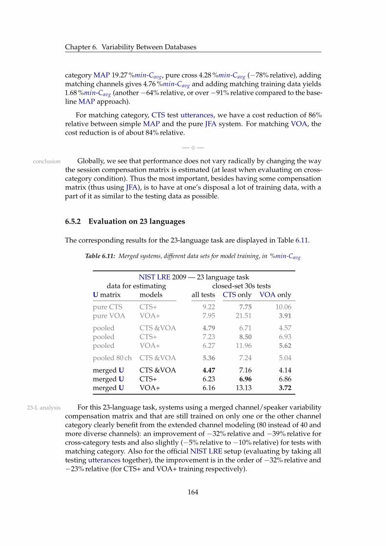
Chapter 6. Variability Between Databases
category MAP 19.27 %min-Cavg, pure cross 4.28 %min-Cavg (−78% relative), addingmatching channels gives 4.76 %min-Cavg and adding matching training data yields1.68 %min-Cavg (another−64% relative, or over−91% relative compared to the base-line MAP approach).
For matching category, CTS test utterances, we have a cost reduction of 86%relative between simple MAP and the pure JFA system. For matching VOA, thecost reduction is of about 84% relative.
— ⋄—
Globally, we see that performance does not vary radically by changing the wayconclusion
the session compensation matrix is estimated (at least when evaluating on cross-category condition). Thus the most important, besides having some compensationmatrix (thus using JFA), is to have at one’s disposal a lot of training data, with apart of it as similar to the testing data as possible.
6.5.2 Evaluation on 23 languages
The corresponding results for the 23-language task are displayed in Table 6.11.
Table 6.11: Merged systems, different data sets for model training, in %min-Cavg
NIST LRE 2009 — 23 language taskdata for estimating closed-set 30s tests
U matrix models all tests CTS only VOA only
pure CTS CTS+ 9.22 7.75 10.06pure VOA VOA+ 7.95 21.51 3.91
pooled CTS &VOA 4.79 6.71 4.57pooled CTS+ 7.23 8.50 6.93pooled VOA+ 6.27 11.96 5.62
pooled 80 ch CTS &VOA 5.36 7.24 5.04
merged U CTS &VOA 4.47 7.16 4.14merged U CTS+ 6.23 6.96 6.86merged U VOA+ 6.16 13.13 3.72
For this 23-language task, systems using a merged channel/speaker variability23-L analysis
compensation matrix and that are still trained on only one or the other channelcategory clearly benefit from the extended channel modeling (80 instead of 40 andmore diverse channels): an improvement of −32% relative and −39% relative forcross-category tests and also slightly (−5% relative to −10% relative) for tests withmatching category. Also for the official NIST LRE setup (evaluating by taking alltesting utterances together), the improvement is in the order of −32% relative and−23% relative (for CTS+ and VOA+ training respectively).
164

6.5. Model level fusion: Merged channel compensation matrices
This observation about the merged-U setup improving in every case for the comparisonto 8-L23-language task could not be confirmed in the "cleaner" 8 language setup, where
the performances with the merged U matrix were very similar to the categoryspecific ones. In that setup, we have all required language–channel combinationsin our training data and thus the additional channels are not of much use. Aninterpretation of this difference between the 8- and the 23-language setups may bethat the data used for estimating the U matrix has at least to cover the language–channel combinations used for model training5.
As we did for the 8-language task, let us have a look at following (pessimistic evolutivesequence:CTS
approach) sequence for the CTS only tests: Cross-category MAP has a min-Cavg
of 35.48% (Sect. 6.2.2), pure cross-category JFA reduces the errors/costs to 21.51 %min-Cavg (−39% relative), adding some matching channels (merged U matrix andstill adverse VOA+ model data) drops to 13.13 %min-Cavg (another −39% relative,or −63% relative from the MAP system) and then adding some channel-matchingdata for model training improves to 7.16 %min-Cavg (additional −45% relative, thatis about −80% relative compared to the adverse MAP system).As difference to the 8-language task, we notice here that adding some channels ofmatching category to the U matrix helps. This means also that JFA does not reallyhelp for channels of non-matching category. The case described here reveals alsothat it is of the same importance to have data of corresponding category in thechannel variability matrix as to have such data for training the models.
Analogously for VOA only tests: Cross-category MAP 27.89 %min-Cavg, pure VOA
cross 10.07 %min-Cavg, adding matching channels gives us 6.89 %min-Cavg (32%relative) and adding matching training data yields 4.18 %min-Cavg (another 39%relative, with totally 85% relative).
The drastic degradation compared to Table 6.10, occurring in a general manner CTSdegradationon the CTS systems (doubling or tripling the number of errors) can be explained by
the fact that in this 23 language case, not even half of the models could really betrained with CTS data (the CTS+ data set containing VOA data for the 12 languagesthat do not have CTS training data).
For the system where CTS+ data was used for model training, the cost for Urdu
the CTS-only tests (matching) is slightly higher than the one of the VOA-only testutterances (cross, on the same models). This can again be explained by the highPmiss of the Urdu language: 65.63% for the CTS&VOA trained system and 71.88% forthe CTS+ one. This finally gives an Urdu CDET of 38.42% and 41.12% respectively(for CDET, see Sect. 2.6.2.2).
— ⋄—
Comparing the results between pooled-U and merged-U matrices seems to model levelconclusionhighlight that the channel variability mapping in the compensation matrix is fairly
5And above analyses seem to indicate that there should be a match between model training andtesting data. The direct link between compensation matrix and testing data seems to be far lessimportant.
165

Chapter 6. Variability Between Databases
on a per-category basis. So adding additional (foreign–category) channels doesnot help in a context where training data of the same category as the test data isavailable for every language (as the more controlled environment of the 8-languagetask). But the additional channels can prove useful when correct channels aremissing from the training data for some languages (23-language setup). Thus themerged-U system proves well when a certain robustness is required.
Looking at the performance on all 30 seconds tests, no single channel dependentsystem performs as well as systems with models trained on all data together.
6.6 Score level fusion: Fully separate category modeling
In Sect. 6.3, we observed that performance is very good when channel compensationsystem selection
matrix, training data and test part are of the same channel-category (matchingcondition). This leads to the question if we could not fuse two completely separatecategory-dependent systems. One of the easiest ways to merge two such completelyseparate systems is by selecting the score that matches the correct channel category.By taking the corresponding system for each testing utterance, this tries to obtainthe benefits of both systems. Thus, in this last approach, the fusion is delayed untilreaching the score level.
So, fully separated CTS and VOA systems are trained and the testing utterancescategorydetector are scored against both systems separately. The idea is then to take, for every single
utterance, only the scores of one or the other system. Ideally, the choice is doneaccording to the real channel category of the testing utterance. In a first run, thisideal choice can be simulated using an oracle, which returns the channel categoryof the utterance.
This section presents and discusses the results using an oracle type selector. Theoracle
oracle tells us of which category the test utterance really is. Our fusion unit thenselects the scores of the corresponding channel-dependent system for that utterance.Since this selector is perfect in terms of channel detection, we can interpret the resultas being the best performance a fusion unit based on automatic channel detectionmay approach. We employ an oracle to investigate the feasibility and the use of asystem combination at this score level.
The separate Chapter 7 will then replace this oracle by automatic channel cate-gory detectors. It will principally dwell on the design of such detectors.
Also for this approach, one problem is the missing training data described inSect. 6.1, which inhibits training a full set of 23 language models for both categories.But we tried to solve this issue by taking data of the other category, where reallynecessary.
166

6.6. Score level fusion: Fully separate category modeling
6.6.1 Evaluation on 8 languages
Table 6.12 evaluates the fusion for the 8-language task. Once, it combines the pureCTS (2.71 %min-Cavg on the matching tests) with the pure VOA (1.90 %min-Cavg
on VOA) systems. This yields a global cost of 2.06 %min-Cavg for the mergedsystem. This result is interesting since it is better than the global results of thesystem merging the channel compensation matrices (merged-U, −12% relative) orthe system pooling all data together since beginning (−7.7% relative). We note alsothat the per-category testing has to produce the same results as the correspondingsingle system (due to the oracle).
The same kind of fusion applied on the category-dependent systems featuringa merged channel compensation matrix performs insignificantly better at 2.04 %min-Cavg, which is 8.6% relative better than the best single system.
Table 6.12: Fusion of JFA systems using an oracle type system selector, compared to best singlesystems, 8-language task, in %min-Cavg
LRE 2009, 8 languagessystem 1 system 2 closed-set 30 s tests
U matrix models U matrix models all tests CTS only VOA only
pooled CTS &VOA 2.23 3.03 1.75merged U CTS &VOA 2.33 3.06 1.68
CTS CTS VOA VOA 2.06 2.71 1.90merged U CTS merged U VOA 2.04 2.61 1.92
We note that the result on all 30 s tests (grouping CTS and VOA segments) candiffer from the value that would be obtained by averaging the matching categoryperformances of the two corresponding single systems (weighted by the number oftests). This happens since the indicated performance uses the average detection costfunction (Cavg) and is thus a mean of language pair (mis-) detection costs, based ona global threshold which may also change from experiment to experiment.
6.6.2 Evaluation on 23 languages
The oracle fusion is also applied on the whole set of 23 languages to match theLRE 2009 protocol. The results using an oracle as selector for fusion are shown inTable 6.13.
The fusion of the two pure systems is with 4.16 %min-Cavg slightly outperformedby the fusion of the systems built on a common, merged eigensession matrix, whichruns at 3.90 %min-Cavg (probably significant −6% relative). This is similar to thedifference that has been observed between unfused pooled and merged-matrixsystems in Table 6.11 (and repeated in Table 6.13). A big part of the easier recognitionon VOA tests is still due to the fact that nearly all language–channel combinations
167

Chapter 6. Variability Between Databases
Table 6.13: Fusion of UBM-based JFA systems using an oracle type selector, compared to best singlesystems, 23-language (NIST LRE 2009) task, in %min-Cavg
LRE 2009, 23 languagessystem 1 system 2 closed-set 30 s tests
U matrix models U matrix models all tests CTS only VOA only
pooled CTS &VOA 4.79 6.71 4.57merged U CTS &VOA 4.47 7.16 4.14
CTS CTS+ VOA VOA+ 4.16 7.75 3.91merged U CTS+ merged U VOA+ 3.90 6.96 3.72
are present in the training data. This fused system with a minimal average cost of3.90 %min-Cavg has a cost reduction of 12.6% relative compared to the best singlesystem with its 4.47 %min-Cavg.
6.7 Channel category conclusion
The data used for the NIST LRE 2009 contains utterances of two different sources:problem
Conversational Telephone Speech (CTS) and Voice of America (VOA). We calledthese two kinds being of different channel categories. We suspected that these twosources have considerably different structures or variabilities. We tried to designan approach which allowed these two categories to be separated. The subsequentanalysis revealing striking differences between these two categories, most notablyin the context of Joint Factor Analysis.
We tried to cope with this category problem by designing parallel category-solutions
specific systems. These systems can be combined together on different levels: 1) Onthe data level, 2) on the model (or more accurately the JFA U matrix) level and 3)
finally on the score level. The data level merging consists in naively pooling all datatogether. With 4.78 %min-Cavg on 2048 Gaussian on the LRE 2009 setup, it achievesalready acceptable performances. The combination on the model level featuresa compensation U matrix, which is obtained by stacking two category-specificones. This systems runs at globally at 4.47 %min-Cavg (−7% relative). Finally, thefusion on the score level analyzed here uses an oracle channel category "detector".Depending on this detector’s output, the scores of one of two category-specificsystems are chosen. The best such combination runs at comparable 3.90 %min-Cavg,which correspond to the middle-field of NIST LRE 2009’s participants. This showsthat it is possible to improve over the naive pooled (JFA) approach (−18% relative).Compared to the baseline MAP approach, this is a reduction of 81% relative.
One important observation of the presented results is that the fact of addingobservations
more data to the U matrix estimation does not necessarily mean an improvement.Certainly, the robustness against testing utterances of a channel category which
168

6.7. Channel category conclusion
was not included in the model training data (cross-category) increases. But thisenhancement comes at the expense of reducing the channel compensation poweron the data of known (matching) category.
But when imposing a certain (a priori) structure on the U matrix, as is forinstance implicitly done when concatenating category-dependent matrices, signifi-cant improvements may be obtained6. This way allows to benefit of the additionalinformation about the other channel category, which can be included into the corre-sponding part of the U matrix. We have further the impression that the VOA partof the compensation matrix slightly overwhelms the CTS one.
One finding was also that the data used for estimating the U matrix has at leastto cover the language–channel combinations used for model training.
In general, the most important bit is to have model training data that is as closeto the testing data as possible. The data used for model training is more crucial thanthe data used for estimating the U matrix.
6Opinion: We think that the two matrices that get stacked may need some proper balancing inorder to benefit fully from both. We tried to normalize each column (corresponding to one channelfactor) individually by its norm. But this strategy was not useful...
169

Chapter 6. Variability Between Databases
170

Les machines un jour pourront résoudre tous les problèmes,mais jamais aucune d’entre elles ne pourra en poser un !
— Albert EINSTEIN
Chapter 7
Channel-Detectors forSystem Selection
Contents
7.1 Designing channel category detectors . . . . . . . . . . . . . . . . 172
7.1.1 Simple-sum . . . . . . . . . . . . . . . . . . . . . . . . . . . 1727.1.2 Feature-based MAP . . . . . . . . . . . . . . . . . . . . . . 1737.1.3 SVM on channel variability . . . . . . . . . . . . . . . . . . 1737.1.4 MAP on channel variability . . . . . . . . . . . . . . . . . . 1737.1.5 Oracle . . . . . . . . . . . . . . . . . . . . . . . . . . . . . . 173
7.2 Novel score normalizations . . . . . . . . . . . . . . . . . . . . . . 174
7.2.1 llkMax0 . . . . . . . . . . . . . . . . . . . . . . . . . . . . . 1747.2.2 llkInt01 . . . . . . . . . . . . . . . . . . . . . . . . . . . . . . 175
7.3 Evaluation on 8 common languages . . . . . . . . . . . . . . . . . 176
7.3.1 Pure systems . . . . . . . . . . . . . . . . . . . . . . . . . . 1777.3.2 Systems with merged-Umatrix . . . . . . . . . . . . . . . . 177
7.4 Evaluation on all 23 languages . . . . . . . . . . . . . . . . . . . . 178
7.4.1 Pure systems . . . . . . . . . . . . . . . . . . . . . . . . . . 1787.4.2 Systems with merged-Umatrix . . . . . . . . . . . . . . . . 179
7.5 Discussion . . . . . . . . . . . . . . . . . . . . . . . . . . . . . . . . 179
If we have rather different channel categories (as analyzed in Chapter 6 for NISTLRE 2009), one possibility is to handle these categories completely separately ina parallel manner and merge such category-dependent systems at the score level.This combination may be done by a system or score selector taking the "better"system for each utterance. This chapter extends this idea of a channel categorydetector, already presented in Sect. 6.6. Here, we replace the oracle based detectorby automatic detectors in different designs.
— ⋄—
171

Chapter 7. Channel-Detectors for System Selection
7.1 Designing channel category detectors
In previous chapter and in (Verdet et al., 2010b), we investigated the idea of model-ing the CTS and the VOA conditions separately. We have shown that the mergingof such separate systems may be done at different levels:
1. Pooling all data together since the beginning (having thus just one commonsystem),
2. stacking channel-category dependent JFA channel compensation matrices (U)in order to have a matrix with a CTS specific and a VOA specific part and
3. merging two completely channel-dependent systems only at the score level.
A simple, but nevertheless effective way to merge such systems at score levelis using a system selector. This means that, for each test utterance, the scores ofone or the other system are taken (selected). Typically, such a system selector actsaccording to the channel category detected in the test utterance and selects thescores of the corresponding system.
In previous chapter, we employed an oracle category detector. The work pre-sented in this section investigates different ways to design automatic channel detec-tors in the context of such a system selector. More specifically, we design channeldetectors based on SDC features (Sect. 3.3.2), as well as detectors working on theJFA level. In the latter variant, the term containing the session variability (the x
vectors of the JFA formula Eq. 4.5) is used. This is a simple, but novel idea, which atthe same time also validates the fundamental idea behind the JFA approach.
The impact of the different channel detectors are evaluated on systems with twodifferent structures, already discussed in Chapter 6:
Pure channel-category systems where the compensation matrix U has a rank of 40and is estimated exclusively on data of one or the other channel category.
Merged-U systems that use a common U matrix, which is obtained by stacking thetwo channel dependent U matrices and has thus a rank of 80. The categorydistinction lies only in the language model training.
— ⋄—
The following sections present the different channel category detectors wedesigned. It is then followed by a comparative analysis presenting results on thetwo category-dependent type of systems.
7.1.1 Simple-sum
The simple sum fusion is not a channel detector, but a baseline replacement forthe system selector. For each test, the scores of both channel-category dependentsystems are summed together (without special weighting). This gives a minimalsystem performance which acts as a baseline for the different channel detectors.
172

7.1. Designing channel category detectors
7.1.2 Feature-based MAP
As a first automatic approach, a Maximum A Posteriori (MAP (Gauvain and Lee,1994)) adapted model is estimated for each of the two categories using all train-ing data (feature vectors) of that channel category. Since the same UBM as fortraining the channel-dependent systems is used, these channel models are mix-tures of 2048 Gaussians. Let us identify this detector by f-MAP . It has a channelidentification rate of 87.63% when evaluated on the 30 second NIST LRE 2009segments.
7.1.3 SVM on channel variability
Since JFA tries to model the session and channel variability separately and expres-sively, it is obvious to try to use this information alone for a channel detector. Thechannel variability part of the JFA formula (Eq. 4.5) is the term Ux. Since U isglobally fixed, the vector x represents the channel variability (the channel factors).In the present setup, these x vectors are obtained in every case using the UBMand the stacked U matrix (Sect. 6.5), since they have to be obtained on a commonU matrix in order to be comparable.
These x vectors (here with a dimension of 40) can directly be used as input SVsfor an SVM (Singer et al., 2003; Campbell et al., 2004; Verdet et al., 2009b). The x
vectors of the target category are taken as positive SVs and the x vectors of the othercategory as blacklist (negative examples). We notice that the two SVMs we get forour two-category case are symmetric (in theory, for a given test, just the sign of theoutput score changes). We shorten this detector as x-SVM and it has a channelidentification rate of 87.41% on LRE 2009 30 seconds.
7.1.4 MAP on channel variability
These FA x vectors can also be used as new features (thus as new front-end) onwhich a new channel-UBM can be estimated. This can then be adapted throughMAP to obtain channel-dependent models working on these x vectors. For the workpresented here, we use models of 64 mixtures (since each utterance is representedby one frame only). This detector returns the channel category corresponding to themodel with the bigger likelihood We write this channel category detector x-MAPand it has an accuracy of 75.29% on the 30 second NIST LRE 2009 segments.
7.1.5 Oracle
The oracle represents the error-less channel detector. It returns the true channel cate-gory of an utterance. Evaluating the systems using the oracle as channel detector,
173

Chapter 7. Channel-Detectors for System Selection
gives the performance we want to approach by automatic channel detectors.
— ⋄—
The performances of automatic data-based channel detectors are thus expectedto lay between the one of a simple-sum fusion and that of the oracle.
7.2 Novel score normalizations
We saw different score normalization strategies in Sect. 2.5.2 and in Sect. 3.5. Whatconcerns inter-utterance normalization, we saw the divSum and the divSum-K ap-proach. The latter requires a constant K to be estimated or empirically chosenbeforehand. This section presents novel approaches to replace this cumbersometechnique. The hypothesis is not to rely on any tunable parameter and to understandwhat is really going on.
7.2.1 llkMax0
The llkMax0 score normalization presented in these lines is also an inter-utterancenormalization, meaning the scores are normalized separately for each test utterance.
Each Likelihood score is divided by the maximum of the scores the utteranceobtains against all language models. Expressed in Log-Likelihood domain, this uni-formly shifts all scores in order to assign a Log-Likelihood of 0 to the hypothesizedlanguage yielding the biggest score (hence the name of llkMax0):
sl(X ) = log
(eLLkl(X )
maxk∈L
eLLkk(X )
)= LLkl(X )−max
k∈LLLkk(X ) (7.1)
where LLkl(X ) is the Log-Likelihood of the utterance X and the hypothesizedlanguage l, whereas L is the set of all languages.
This procedure has the effect of aligning the top-scores of all utterances to aDET step
Log-Likelihood of 0 (or 1 in Likelihood domain). De facto, this accepts all highestscores, producing a minimal level of false acceptance rate1.
The problem of setting the threshold thus exploits principally the informationfocus
about the second-biggest score. If the second-biggest score of an utterance lies nearto the biggest one (thus rather near to 0), it will pass to the positive side of thethreshold sooner than if its distance to the biggest one was larger. Hence the basicidea behind this approach is to focus mainly on the second-biggest scores. The
1While lowering the threshold from the high end (imagine the DET plot), the progress of the falseaccept rate will jump from 0 to this minimal level. Then, it potentially stays at this level for somerange. This produces a rectilinear step on the DET plot. The threshold at this edge point lies hence at(normalized) score 0.0.
174

7.2. Novel score normalizations
assumptions are the following: (i) If the biggest corresponds to the true language,we are on the safe side (de facto acceptance). (ii) If the true one is not the biggestone (the recognition was not optimal), the chances that it is the second-biggest ishigher if the spacing between these two top scores is relatively small.
Fig. 7.1 (a) shows the distribution of llkMax0 normalized scores of a typical JFAexperiment. Note that the big (target) peak as result of the 0.0 alignment is cut offsince it extends to some big value2. We see that the false acceptance peak of thenon-targets is far smaller3. Compared to the non-targets, the targets that did notmake it to 0 (thus second-biggest and beyond, here accounting for 16.8% of thetargets) are all relatively proximate to 0. In fact, the distributions resemble to theones of divSum-K in Fig. 2.7 with a K high enough.
— ⋄—
We looked for a simpler scheme than the division by the sum put to a power of K(divSum-K ) described in Sect. 2.5.2.2 in order to avoid having to tune the parameterK. The simple division proposed here has the big advantage not to depend onany tunable parameter, nor on the availability of a separate calibration dataset (asrequired for more evolved back-ends like the GBE). Nevertheless it still performs aswell as the divSum-K approach.
The basic idea behind this llkMax0 score processing is mainly to exploit theconstellation of the few highest scores of each utterance (mainly the second-highest).This kind of score normalization is used throughout the current chapter.
7.2.2 llkInt01
In last section, we presented the llkMax0 approach with the big advantage to performas well as divSum-K , but not requiring any parameter (K). Here, we presenteven an other approach, which can be logically derived from divSum-K . But thechronological development was inverse since this llkInt01 normalization process asdesigned by Jasmin Wei Ming Liu4, whose idea was then spun further.
— ⋄—
The principle of llkInt01 is not only to put the highest score to some fixed value,but doing similarly for the minimum. This transforms the set of (Log-Likelihood)scores of one utterance to a fixed interval, namely 0 to 1. (We note that in thiscase, we can not see the result as being Log-Likelihood-like any more, but a moreappropriate interval could have been chosen.)
2In the present case up to over 83003Here fitting on the plot with 35.34Affiliated to Ultra Electronics AudioSoft and to the University of Swansea.
175

Chapter 7. Channel-Detectors for System Selection
The scores are thus shifted and scaled as follows:
sl(X ) =LLkl(X ) −mink∈L
[LLkk(X )
]
maxk∈L
[LLkk(X )
]−mink∈L
[LLkk(X )
] (7.2)
where LLkl(X ) is the Log-Likelihood of the utterance X and the hypothesizedlanguage l, and L is the set of all languages5.
Fig. 7.1 (b) gives an idea of the score distribution after llkInt01 normalization forthe same system as in (a) and in Fig. 2.7. Here again, the y-axis is truncated6.
— ⋄—
The approach presented here formed the basis for the thoughts, which lead tothe llkMax0 technique described in Sect. 7.2.1. The results using this approach hereare slightly better than the bare divSum approach, but not as good as divSum-K .This can principally be funded on the problem induced by aligning the minimum.The minimal scores do not have (or has only very little) influence on thresholding.The minimum more depends on the set of languages in our task. It is more thehigh-scoring range which is decisive.
0
5
10
15
20
25
30
35
40
-0.16 -0.14 -0.12 -0.1 -0.08 -0.06 -0.04 -0.02 0
p(s
co
re)
score
targetsnon-targets
(a) llkMax0
0
1
2
3
4
5
6
7
0 0.2 0.4 0.6 0.8 1
p(s
co
re)
score
targetsnon-targets
(b) llkInt01
Figure 7.1: Sample score distributions for llkMax0 and for llkInt01 normalized scores for our JFAsystem
7.3 Evaluation on 8 common languages
The results presented subsequently are based on SDC features. All models aresetup
obtained through MAP adaptation from the UBM with JFA channel and speakernormalization. All models are composed of 2048 Gaussians. Data parts and generalsystem structures are the same as in Chapter 6, following the NIST LRE 2009protocol and adding an 8-language task. The results presented in this section arebased on scores which are normalized using the llkMax0 approach (Sect. 7.2.1)7 and
5As degenerate case of all scores happening to be the equal (possible consequence of an utterancecontaining no speech), the denominator is set to 1 — so that the resulting scores are all equal to 0.
6At the 0 edge, where the minima are aligned, the non-targets reach about 137 in the present case.At the 1 edge of the maxima, the targets reach 2.3 · 109 and the non-targets as indicated 5.6.
7This change in normalization strategy accounts for the very slight change of the values comparedto last chapter.
176

7.3. Evaluation on 8 common languages
evaluated under the min-Cavg measure.
As explained in Sect. 6.1, there are some language–channel combinations which 8-L task
lack training or testing data. This section thus evaluates the systems on the NISTLRE 2009 30-second segments of the 8 common languages only, as well as solely onthe CTS and solely on the VOA subset.
7.3.1 Pure systems
Table 7.1 presents the results of the two pure channel-category dependent systemsand their fusion. The results of all automatic channel detectors fall in between thoseof a simple-sum fusion and the oracle. We observe that the best results among theautomatic channel detectors are obtained by the x-SVM detector. They approachthe ones of the oracle, which represents ground truth, quite well (only ∼6% relativefrom the oracle away). The weakest channel detector is the one where the samex vectors are modeled by MAP.
Table 7.1: 8 languages, pure per-channel systems, in %min-Cavg
LRE 2009 closed-set 30sbase system fusion all 30s tests CTS tests only VOA tests only
CTS — 2.34 2.11 2.94VOA — 6.34 9.88 1.28
— simple-sum 2.58 3.67 1.30— oracle 1.63 2.11 1.28— f-MAP 1.88 2.49 1.38— x-MAP 2.31 3.06 1.73— x-SVM 1.73 2.27 1.26
7.3.2 Systems with merged-Umatrix
The results shown in Table 7.2 are obtained by systems featuring a common mergedU matrix. This matrix is obtained by stacking the two channel-dependent U matricesused for the pure systems. The observations for the merged-U systems are similarto those for the pure systems. Except for the VOA only evaluation, we identify aclear general tendency of slightly better performances for these merged-U systemscompared to the pure category systems (i.e. with 4.3% relative gain for the x-SVMchannel detector). When evaluated on the channel-categories separately, the featurebased MAP detector (f-MAP ) is slightly better than x-SVM with 2.30 %min-Cavg forCTS tests and 1.44 %min-Cavg for VOA tests.
Evaluated on all 30-second segments, system selection based on the x-SVMchannel detector have a minimal average cost of 1.65%, which is respectable −90%
177

Chapter 7. Channel-Detectors for System Selection
relative over the most basic MAP system (trained on all data pooled together).
Table 7.2: 8 languages, merged-systems, in %min-Cavg
LRE 2009 closed-set 30sbase system fusion all 30s tests CTS tests only VOA tests only
CTS — 2.53 2.04 3.63VOA — 6.30 6.64 1.48
— simple-sum 2.40 3.48 1.60— oracle 1.55 2.04 1.48— f-MAP 1.75 2.30 1.44
— x-MAP 2.27 2.96 1.87— x-SVM 1.65 2.39 1.45
7.4 Evaluation on all 23 languages
This section now presents the same systems under the 23 language NIST LRE 2009task. It also shows to which extent the systems are robust enough to recognizelanguages of a channel category for which no training data is available.
7.4.1 Pure systems
The results in Table 7.3 show that the automatic channel detectors achieve resultsthat are a bit further off the oracle (about 12% relative) compared to the 8-languageprotocol, but they remain clearly closer to the oracle than to the simple-sum perfor-mance.
Table 7.3: 23 languages, channel-dependent , in %min-Cavg
LRE 2009 closed-set 30sbase system fusion all 30s tests CTS tests only VOA tests only
CTS — 9.87 7.44 11.05VOA — 8.59 25.40 3.73
— simple-sum 8.70 16.73 6.39— oracle 3.95 7.44 3.73— f-MAP 4.47 8.24 4.02
— x-MAP 5.94 9.84 5.51— x-SVM 4.65 8.35 4.36
178

7.5. Discussion
7.4.2 Systems with merged-Umatrix
The performances of the systems using a common stacked U matrix are given inTable 7.4. As for the 8-language task, they also indicate that these systems performbetter than the pure systems. The f-MAP channel detector performs best with its3.85 %min-Cavg. Its enhancement over the channel-category dependent U matrix(pure) systems is 14% relative. Compared to the simplest MAP system, this showsan improvement of over 81% relative for all 30-second test utterances.
Table 7.4: 23 languages, merged-systems, in %min-Cavg
LRE 2009 closed-set 30sbase system fusion all 30s tests CTS tests only VOA tests only
CTS — 6.59 6.63 7.51VOA — 5.80 13.77 3.43
— simple-sum 4.32 7.17 3.92— oracle 3.64 6.63 3.43— f-MAP 3.85 7.01 3.54
— x-MAP 4.78 7.58 4.51— x-SVM 4.44 7.58 4.09
7.5 Discussion
All these results show that channel detectors may be designed in different waysand that they may approach the performance of oracle based ground truth fusionup to 5–6% relative.
Of the analyzed channel detectors, x-SVM and f-MAP achieve similar perfor-mances. Whereas the former performs marginally better when training data for allchannel-categories (and languages) is available and the latter seems more robust toincomplete data.
The results on the x vector based detectors confirm the basic idea behind JointFactor Analysis, in which the channel variability is captured by the Ux term ofEq. 4.5.
The validation of x vector based channel detectors opens the important and perspectives
interesting perspective of completely data driven systems that automatically clusterand identify channel categories in the training data (instead of having the labelsabout CTS and VOA). This is not possible on the feature level, since the informationabout the channel (and thus about the channel category) is mixed up with theinformation about the language itself. But the channel category detectors based onthe x-vectors make this possible.
179

Chapter 7. Channel-Detectors for System Selection
Opinion: Even better results may be obtained upon employing more sophisti-cated back-ends. But these require separate development data for estimatingtheir parameters.
180

L’ampule électrique n’a pas été inventéeen perfectionnant la bougie !
— Unknown colleague assistant,on the why of research, CIES, 2009 0
Chapter 8
Perspectives
Contents
8.1 Development set . . . . . . . . . . . . . . . . . . . . . . . . . . . . 181
8.1.1 Chunked training files . . . . . . . . . . . . . . . . . . . . . 182
8.2 Higher level approaches . . . . . . . . . . . . . . . . . . . . . . . . 183
8.2.1 Signal dynamics on Gaussian indices . . . . . . . . . . . . 183
8.2.1.1 Possible implementation . . . . . . . . . . . . . . 186
8.2.2 Pair-wise SVMs . . . . . . . . . . . . . . . . . . . . . . . . . 187
8.3 More technical directions . . . . . . . . . . . . . . . . . . . . . . . 188
8.4 Conclusion on perspectives . . . . . . . . . . . . . . . . . . . . . . 189
In this chapter, we will give some thoughts about what additional elements mayhave been tried and which are likely to enhance results or solve spotted problems.We will also discuss some bigger research directions, which may deserve furtherinvestigation.
8.1 Development set
We saw two kinds of normalization on the score level: inter-utterance and inter- inter-languagenormalizationlanguage normalization (Sect. 2.5.2), the latter including more elaborate back-ends.
Such inter-language techniques try to even out the strengths of the different lan-guage recognizers (models). They usually depend on some previously estimatednormalization parameters. The different analyses on this topic conducted duringour works turned out that this style of normalization made certain demands on thedata set used for estimating these parameters.
— ⋄—
0English transition: The electric bulb has not been invented by perfecting the candle!
181

Chapter 8. Perspectives
Ideally, the data which is run through the system to obtain scores on which thesedev set
parameters are gathered comes from a spare data set. This is usually done this waybecause we assume that a certain structure, which is captured by the modelizationstep, gets also expressed in the scores. For instance, data which is hard to model oroutliers to the modelization is also likely to have bad scores. Score normalizationwith parameters estimated on the same data set as the models may even reduce theuniversality or robustness (appropriateness to slightly different data) for the testingstep.
The parameters for such score calibration should be estimated using a separatedata set, commonly called development set. In the current setup, we did not keepapart some part of the data for this and included all available parts for estimating themodels and the variability matrix at best. In early stages, we were not completelyaware of the importance of score calibration (or inter-language normalization). Onlywith concentrating our attention to the score processing step, we saw that betterresults could probably have been obtained using a more evolved back-end (BE). Inthe context of LRE 2009, (Jancik et al., 2010) investigated different compositions forthe development set.
Several tests and analyses1 were carried out to put into action an inter-languageanalyses
normalization BE using the training set instead of a development set. But all resultsyield performances at the same level or marginally poorer.
— ⋄—
A proper score normalization is crucial for obtaining good results. Even if wespent enough time on this part of the system, which does not lie in the core topic ofthis thesis, a better approach should be chosen. Some development data set shouldbe defined and typically a Gaussian Back-End (GBE) based processing pipeline(Sect. 3.5.2.1) should be applied. This could potentially lead to a system withincreased performance, to a system with less loss due to calibration (see Sect. 3.6.1for this concept).
8.1.1 Chunked training files
When trying to add a back-end (GBE or similar) to our system by estimating itsparameters on the training data itself, we run the training utterances as if theywere testing segments through our system. Having thus the scores of the trainingutterances, we may analyze the "quality" of training (possibly biased by overfitting)by calculating the system performance on these (known) utterances. Doing so, weobserve that only a very few (typically 0, 1 or 2) errors are made on the whole setand that all other utterances are recognized correctly. This happens on the LRE 2005protocol, where only CallFriend data is used in the training phase.
There seems to be two reasons for these good results on the training data itself:number ofutterances
1These range from a kind of simple Tnorm, over the use of FoCal (FoCal, 2007), to Logistic
182

8.2. Higher level approaches
The first is that there is only a very limited number of utterances in this (CallFriend)training set, namely 120 or 240 per language, which is a total of 1 200 over all sevenlanguages. This is potentially too few for a good estimation of BE parameters.
As second reason, these CallFriend files contain each about 14 min of speech, duration
since they originate from half-hour telephone conversations. This is far more datathat is at the recognizer’s disposal than in the real testing utterances with 30 s(or 10 or 3 s resp.). On this side, the fact that an elaborate BE does not give anyimprovement may also be due to this difference in length between the training(or calibration training) and testing utterances. A difference in duration from thetraining to the testing data may also introduce some bias to the results — this isparticularly true for SVMs (see discussion of SVMs in Sect. 5.4.1).
One solution (while sticking to the training data) would be to cut each utterance solution/resultsinto smaller parts to be handled individually. This procedure was attempted in
some early stage by extracting segments containing at least 30 s of speech from theCallFriend utterances. The individually applied mean and variance normalization(feature level) did not show any effect to the modelization (and hence to the results).Also, the JFA step estimating the U matrix using these shorter utterances showeditself insensitive to this change. Due to these reasons, this procedure chopping thelong utterances into shorter ones was left apart in later development and it was notre-attempted for the BE normalization. But this surely constitutes a possible way ifwe want to add a more evolved BE.
As a reference to other works choosing this chopping approach, we may cite(Castaldo et al., 2007c), which split the same CallFriend utterances into 8172 chunksof about 150 s each.
8.2 Higher level approaches
In this work, we focused on GMM based acoustic modeling. This could form thebasis of a vast diversity of further researches exploring higher level information, butkeeping the basic core of the system simple and based on such short time acoustics.
The following sections will shortly present some ideas of such short time acous-tics based higher level systems.
8.2.1 Signal dynamics on Gaussian indices
We saw that each feature vector can be seen as a point in multidimensional space. multi-dimensionalpath
A speech utterance, which consists of a series of feature vectors, can be representedas a sequence of points. Since the signal is thought to be quasi-stationary andcontinuous on a very short term, the values of adjacent feature vectors change only
Regression or LDA + Gaussian modeling.
183

Chapter 8. Perspectives
slightly (i.e. this is exploited by the deltas). So an utterance can be seen as a (moreor less continuous) path through this multidimensional space.
— ⋄—
We assume that this path can be discretized by keeping for each frame only theGaussianindices index (identity) of the Gaussian of a previously trained model, whose distance to
the frame is minimal (also called the top-1 Gaussian). For this, typically the UBM isused.
First analyses show that using only the top-N Gaussians in a usual JFA basedtop-N
system is enough to achieve equal or similar performances as when using allGaussians. These results are sketched in Table 8.1 for a 256 Gaussian system usingthe accurate JFA strategy. We observe that even when limiting to only one Gaussian,the systems does not loose too much of its power. This is a first validation step forthe described assumption.
Table 8.1: Effects of using only the top-N Gaussians, tested on NIST LRE 2005, in %pooled EER
Top-N 1 3 6 10 15 20 30 50 100 256%EER 11.43 9.00 8.86 8.85 8.86 8.86 8.86 8.86 8.86 8.86
Having "decoded" all utterances into sequences of Gaussian indices, we maytransitionhistograms analyze these sequences. For instance, we may calculate, for each language sepa-
rately, the frequencies of transitions from one index to another along these paths.During testing, we may re-use these statistics to calculate a Likelihood score (in astraightforward manner).
As a next step in development, we may build statistics on the duration a pathdwellingdurations "dwells" around a given Gaussian. This tracks the number of consecutive indices of
the same value. For each Gaussian of each language, we will obtain a histogram ofthe frequency as function of the dwelling duration (this is illustrated in Fig. 8.1 (a) ).We assume that the histograms for some Gaussians sensibly differ from languageto language. The problem here is surely the jitter in the index sequence. We mayperhaps apply some smoothing to the sequence beforehand (slightly similar to thesmoothing in the SAD step, Sect. 2.3.2).
These duration histograms may be transformed to complementary cumula-minimumduration tive distributions, which indicate how much time (in number of frames) the path
dwells at least on a given Gaussian (thus the sum from n to positive infinity in theabove histogram). This is called Minimum Duration Modeling (MDM) and otherapplications of it (without references here) indicate that such a distribution cantypically be divided into two zones: (i) a high (cumulative) probably zone for lowminimal durations (meaning that only a very few sequences are that short) and (ii)after a certain edge point, the complementary cumulation seems to decrease in anasymptotic manner. More accurately, it is most likely a complementary Gumbel
184

8.2. Higher level approaches
cumulative distribution (also Gumbel survival function for the maximum case)2.This is illustrated in Fig. 8.1 (b). We assume that this minimal duration thresholdpotentially changes from language to language. The modeling is thus built aroundthis threshold3.
As consequence, we may use this MDM to force the path to dwell on a given forced MDM
Gaussian for (at least) the number of frames, which corresponds to the minimalduration threshold. This forcing can be used for instance in conjunction with classicLikelihood calculation (Sect. 2.5.1), where the posterior probability γ of this possiblyforced Gaussian is used. For the true language, this constraint should not inducesevere penalties, but for false languages, this is likely to introduce potentially severeloss in Likelihood. MDM enforcing imposes the use of bad or very bad Likelihoodvalues for some frames if the forced Gaussian does not correspond to the top-1Gaussian. Fig. 8.1 shows in (c) the top-1 Gaussian for each frame (dark-gray boxes)and the Gaussians forced by MDM (black connected boxes).
One problem of such an approach is the dependence of the starting point for the problem
forcing — which frame we start with. We propose for instance to apply a thresholdon the frame Likelihood, which has to be exceeded for the MDM to apply (on thefollowing frames).
p
duration [frames]
1 2 3 4 5 ...
...
fr, g1
(a) Duration histogram
duration [frames]
1 2 3 4 5 ...
...
100%
minimal duration
fr, g1
(b) Minimum duration
frames
likelihoodGaussian|frametop-1
x=1 2 3 ...
G123
...
likelihoodGaussian|frameforced MDM
G123
...
(c) Forced MDM
Figure 8.1: Illustration of the different statistics for a given language and a given Gaussian in (a),(b)and the MDM forcing imposing penalizing Likelihoods in (c)
2The Gumbel distribution is also known as the log-Weibull distribution or the type I extremevalue distribution. See also http://en.wikipedia.org/wiki/Gumbel_distribution andhttp://www.itl.nist.gov/div898/handbook/eda/section3/eda366g.htm
3Apparently, some researchers choose as minimal duration threshold half the value of the averageduration.
185
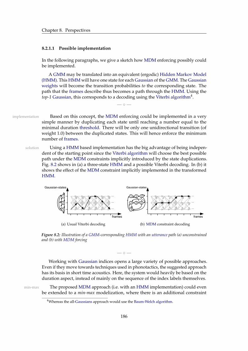
Chapter 8. Perspectives
8.2.1.1 Possible implementation
In the following paragraphs, we give a sketch how MDM enforcing possibly couldbe implemented.
A GMM may be translated into an equivalent (ergodic) Hidden Markov Model(HMM). This HMM will have one state for each Gaussian of the GMM. The Gaussianweights will become the transition probabilities to the corresponding state. Thepath that the frames describe thus becomes a path through the HMM. Using thetop-1 Gaussian, this corresponds to a decoding using the Viterbi algorithm4.
— ⋄—
Based on this concept, the MDM enforcing could be implemented in a veryimplementation
simple manner by duplicating each state until reaching a number equal to theminimal duration threshold. There will be only one unidirectional transition (ofweight 1.0) between the duplicated states. This will hence enforce the minimumnumber of frames.
Using a HMM based implementation has the big advantage of being indepen-solution
dent of the starting point since the Viterbi algorithm will choose the best possiblepath under the MDM constraints implicitly introduced by the state duplications.Fig. 8.2 shows in (a) a three-state HMM and a possible Viterbi decoding. In (b) itshows the effect of the MDM constraint implicitly implemented in the transformedHMM.
1
2
3
...
...
...
Gaussian-states
frames
(a) Usual Viterbi decoding
...
...
...
1
2
3
2 2
1 1
Gaussian-states
frames
(b) MDM constraint decoding
Figure 8.2: Illustration of a GMM-corresponding HMM with an utterance path (a) unconstrainedand (b) with MDM forcing
— ⋄—
Working with Gaussian indices opens a large variety of possible approaches.Even if they move towards techniques used in phonotactics, the suggested approachhas its basis in short time acoustics. Here, the system would heavily be based on theduration aspect, instead of mainly on the sequence of the index labels themselves.
The proposed MDM approach (i.e. with an HMM implementation) could evenmin-max
be extended to a min-max modelization, where there is an additional constraint
4Whereas the all-Gaussians approach would use the Baum-Welch algorithm.
186

8.2. Higher level approaches
indicating the maximum duration. As a hint, this could be implemented by re-placing the state which has a (non-zero) self-transition by a series of (left-to-right)states with jumping (or by-passing) transitions (removing the self-transition avoidslooping of uncontrolled length).
An extended discussion of all ideas introduced in this section has been formu-lated in (Verdet and Hennebert, 2010).
8.2.2 Pair-wise SVMs5
We investigated SVMs in Chapter 5. Since SVMs are binary classifiers, but we areworking in a multi-class environment, we took the approach were we estimatethe hyperplanes using one target language and putting all other languages to thenegative class.
We may likewise train a set of pair-wise SVMs, meaning that their hyperplanes pair-wise SVMs
are estimated using SVs of two languages only: the hypothesized as positive andone other language in turn as negative class. The hypothesis is that such SVMs canbe estimated more robustly than if we had SVs of |L| − 1 languages on the negativeside.
Working with L languages, we end up with|L| · (|L| − 1)
2pair-wise SVMs, if we ergodic vector
do all combinations. As a first approach, the Likelihoods of an utterance run againstall these SVMs may get concatenated into one big score vector, which can be inputto a back-end (BE) to obtain a series of |L| final scores. This will probably exploitthe constellation of the utterance in the multidimensional space of all languages ina better way as can be achieved with one-against-others SVMs.
The vector of pair-wise SVM scores may also be augmented for instance byclassical GMM (-JFA) scores before being input to the BE. The expected effect wouldbe the SVM scores giving additional guidance in the case where the GMM ones arenot clear enough (i.e. the highest Likelihood not standing out against the others). Inorder to avoid to have too large score vectors, we may also take only some selectedpair SVMs. For instance those of often confound languages. As a development, wemay also think of a more complex architecture which uses only a few automaticallychosen SVMs. I.e. taking only those with big Likelihoods, thus those in which wehave a sufficient confidence in order to enhance the GMM based detection.
These pair-wise SVMs may for instance also be exploited in some hierarchic hierarchy
manner, deciding at each level towards the more likely language or by introduc-ing some bonus system, giving more weight to the languages that obtain betterlikelihoods against many other languages.
5These pair-wise SVM based findings were sketched in an exchange with Jasmin Liu, affiliated toUltra Electronics AudioSoft and to the University of Swansea.
187

Chapter 8. Perspectives
8.3 More technical directions
RaSta-PLP-SDC
In Sect. 3.3.3, we compared parameterizations with different compositions of indi-vidual processing steps. From Table 3.3, we see that we missed out one interestingand promising combination. As basic type of features, PLPs seem very promising.We saw also that as well RaSta filtering normalization, as also the addition of delta-blocks (to obtain SDCs) show beneficial. The idea is then to combine these threeelements to RaSta-PLP-SDC features.
Analysis of accurate JFA approach
While looking back to our work, we noticed that it would be interesting to analyzethe effects of the U matrix rank, as it is done in Sect. 4.4.2, but for the accurate JFAapproach (described in Sect. 4.3.3). The results are potentially different from thoseusing the approximated JFA. We may guess that while lowering the number ofchannels (U rank), the accurate JFA will still work good enough for longer (lowerranks) than the approximate one. If this is the case, the justification may be that theaccurate way is able to exploit the (few) channels in a better way.
Enhanced category detector
On the channel category detector side, the next potential step would be to includef-MAP +JFA
the JFA technique to the f-MAP detector. The disturbing variability we want toremove will then be the intra-category differences. Here, it will be constitutedof the information about the language, the speaker and the fine-grained channelfluctuations.
As a second future direction may be imagined to design a system, which obtainsx-* from fulldecomposition cleaner category-dependent factors (x) for the x-MAP and x-SVM detectors. More
category-specific x factors may for instance be obtained (i) by the JFA approachusing intra-category variability, as described in last paragraph or (ii) maybe evenbetter would be to use a full decomposition, as described in Sect. 4.1.1. This wouldseparate the nuisance information into multiple terms, each of which lives in aseparate subspace. One of these (specialized) subspaces will then correspond to thechannel category, whereas the other disturbing information is constraint to differentsubspaces.
The full decomposition is likely to enhance the accuracy of the channel categoryproblems
detectors, but at the cost of much more engineering (i.e. estimating a differentmatrix for each subspace). In addition, this complete decomposition will void theperspective about partitioning the training data into automatically determined,data-driven channel categories since the decomposition into multiple subspacesrequires labels for the different subspaces. We may at most choose a data-drivenapproach as first layer (a kind of bootstrapping) to produce labels (of the channelcategory) and then to use a multi-subspace approach in a second turn in order torefine the categories and the recognizer.
188

8.4. Conclusion on perspectives
8.4 Conclusion on perspectives
Even though Feature Extraction was not part of the core subjects of this thesis, FE
we think that some more enhancement could be reached in this domain. Wemay try more ingenious SDC building strategies in the neighborhood of silencesegments, where frames labeled with silence are used for building delta-blocks.Likewise, we may give a try to T-DCT type features (Kinnunen et al., 2006; Castaldoet al., 2007c) since they operate comparably to the SDCs, but use all frames withinthe "lookahead" window and may avoid the second problem of SDCs, which isrepeating delta-blocks.
We have also the feeling that we did not reach the best Speech activity detection SAD
(SAD). We showed in Sect. 2.3.2 that SAD can have a crucial impact to performance.
For being able to balance the different language recognizers among themselves, dev set
a development dataset, as well as more complex BE modules are necessary. Firsttries indicate however that a Gaussian Back-End alone is not able to do such inter-language normalization.
Although SVMs are nowadays outrun by other algorithms, we may also advance pair-wise SVMs
on this path. We suppose that pair-wise SVMs may give additional information incontexts of uncertainness.
A great share of research may be carried out on higher level approaches whichbuild on the short time acoustic features we researched here. We may discretize the Gaussian
indicesutterances into a sequence of Gaussian indices, representing the utterance as a tra-jectory in multidimensional space. Having partitioned this space into (discretized)areas, we can gather statistics on the number of consecutive frames spent in eacharea. This leads to Minimum Duration Modeling (MDM), which can then be usedto force utterances of false languages to a penalizing trajectory.
This chapter presented some thoughts and first analyses of how future researchdirections, which are based on the present thesis, may look like.
189

Chapter 8. Perspectives
190

Je ne vous dis plus rien ; la vertu, quand on l’aime, porte denos bienfaits le salaire elle-même. Mon admiration, monrespect, mon amour, voilà ce que je puis vous offrir en ce jour.
— Pierre Carlet de Chamblain de MARIVAUX,Annibal, 1720, Acte V, Scène 4
Chapter 9
Conclusion
Contents
9.1 Language recognition and variability . . . . . . . . . . . . . . . . 191
9.1.1 Challenges and solutions . . . . . . . . . . . . . . . . . . . 191
9.1.2 Troublesome variability . . . . . . . . . . . . . . . . . . . . 192
9.1.3 Acoustic language recognition . . . . . . . . . . . . . . . . 193
9.2 Novelties . . . . . . . . . . . . . . . . . . . . . . . . . . . . . . . . . 193
9.2.1 Joint factor analysis . . . . . . . . . . . . . . . . . . . . . . . 194
9.2.2 Support Vector Machines . . . . . . . . . . . . . . . . . . . 196
9.2.3 Channel category variability . . . . . . . . . . . . . . . . . 196
9.2.4 Channel category detectors . . . . . . . . . . . . . . . . . . 197
9.3 Wrap-up . . . . . . . . . . . . . . . . . . . . . . . . . . . . . . . . . 198
9.1 Language recognition and variability
Language Recognition is the problem of discovering the language of a spokenutterance. If a person is familiar to the language, the recognition is quite easy. If heknows other languages of the same family, he may still guess which language it is.
A particular domain of computer science tries to recognize the language con- field of research
tained in a speech utterance by automatic means. Such research is part of the vastfield of automatic speech processing, which also includes speech recognition andSpeaker Recognition
9.1.1 Challenges and solutions
The definition of the Language Recognition (LR) task itself comes along with challenges
some challenges. Dialects, non-native accents and foreign words make it difficult.
191

Chapter 9. Conclusion
Furthermore, it may also have to operate in a multilingual environment. To themain applications can be counted telephone based voice servers, video recordingtagging and national security applications.
We presented some basic requirements of automatic speech processing systemssystemcharacteristics and enumerated the conditions an automatic Language Recognition (LR) system
should fulfill, together with the difficulties to meet them. An LR system shouldnamely be designed in a way which makes it being independent of following points:the pronounced content, the application context, the style of speech, the acquisitionand transmission, the signal quality, the set of targeted languages and the speaker.With respect to these basic requirements, it should first and foremost be easilyextensible to additional languages and come along with substantial robustness tochanging conditions like the speaker or the microphone. Keeping the extensibilityof existing systems, this thesis focuses on the robustness of Language Recognitionsystems.
We gave an overview over automatic Language Recognition systems. A shortapproaches
outline of diverse existing approaches was given. Such systems can be distinguishedby the linguistic level they operate on: acoustic systems analyzing the sound of alanguage, phonetic systems using occurrence statistics of phones and phonotacticsystems tracking the sequence of phones/phonemes. Other approaches observethe prosody or operate on the morpho-lexical and syntactical level. For the workspresented herein, acoustic systems (which operate on the lowest level) have beenchosen, since they easily meet the extensibility condition.
9.1.2 Troublesome variability
The robustness term is highly linked to the concept of variability. In an LR system,variability
there is a lot of parts which may have considerable variability. This includes theinherent differences between speakers, the evolution of each speaker, the dialects oraccents (in the case they are not required to be distinguished) and the variabilitiesdue to the acquisition and transmission of the signal.
All these variabilities have a penalizing effect to automatic systems. Generally,the separability of the different classes (here the languages) is reduced by thesenuisances. This is the main problem we observe in the data and it constitutes achallenging environment. The approaches investigated in this thesis follow the goalof taking into account this variability.
This variability problem is similar to the one that Speaker Recognition (SR)factor analysis
has to face, but its nature is slightly different. While the information about thespeaker is the important piece in SR, it is part of the nuisance in the LR domain.Nevertheless, we adapted and applied the Joint Factor Analysis (JFA) concept,which works well in SR, to our domain. This solution consists in decomposingthe information contained in the acquired signal into three components of differ-ent levels: a global component (an overall mean), a language-specific part andthe language-independent nuisance part. The decomposition permits to model
192

9.2. Novelties
explicitly this last variability part. This way, we can compensate our system for theestimated variability and obtain enhanced results.
9.1.3 Acoustic language recognition
In Chapter 2, we presented the whole processing flow of a system modeling acousticmodelinglanguages on the acoustic level. As most of the typical pattern recognition systems,
it is divided into two consecutive phases: the training where for each class themodel parameters are estimated and the testing phase where these models are usedto score data of unknown class.
In both phases, the first step always consists in Feature Extraction (FE), which FeatureExtractioncuts down the input signal into a more manageable representation. Traditionally,
the frequencies contained in the signal are extracted and transformed to a cepstralrepresentation, the feature vectors. A first step of normalizations may be carriedout at this stage, like CMS, VTLN or RaSta.
In the training phase, one model for each class (language) is estimated. In the training
acoustic modeling approach we have chosen, these are Gaussian Mixture Models(GMMs), which are derived from the Universal Background Model (UBM) througha MAP criterion. For the development of the further approaches, we used GMMs of256 components, whereas full evaluation models consisted of 2048 mixtures.
In the second phase, the extracted features are scored against each model in testing
turn. This produces a (Likelihood) score as output. Subsequent score processingsteps like score normalization and calibration are generally applied before they areused to take a decision. This has the effect of putting the scores of the diverse testingutterances to a common range and to achieve some balance between the differentlanguage models.
If the system is run in an evaluation objective, the outputs of a big number evaluation
of tests are analyzed in order to give a performance measure. We also gave anoverview over different ways to measure the performance. The Equal Error Rate(EER) measure is not well adapted for this, since it becomes biased if the differentclasses do not have the same number of testing utterances. One of the most suitableand unbiased methods is the minimal average cost (min-Cavg).
9.2 Novelties
The main challenge handled by the thesis consists in the unwanted variabilitycontained in the data, which is mixed up with the useful language-dependent infor-mation. In a first step, we largely discussed the proposed Joint Factor Analysis (JFA)approach, which has been borrowed from researches in the Speaker Recognitiondomain.
193

Chapter 9. Conclusion
We applied JFA to UBM-based GMMs using a Likelihood scoring, as well as toSupport Vector Machines (SVMs) originating from such GMMs. This analyzes thepossibly to use JFA as a global approach, which can get hold of diverse variabilities.In an other optic, we also probed to apply JFA by building differentiated systems,for telephone and for broadcast based sources.
9.2.1 Joint factor analysis
In Chapter 4, we thoroughly described the concept behind JFA. The main assump-decomposition
tion behind the JFA approach is that the information contained in the observedutterance can be separated into multiple components. The most important decom-position consists in separating the language-independent information from thelanguage-dependent one. Additionally, this language-dependent part is furtherdecomposed into a globally valid part and a purely language-dependent term.
Formally, this decomposition can be written as (Eq. 4.5):decompositionimplementation
m(h,l) = m + Dyl + Ux(h,l) (9.1)
During the training phase, the different terms can be obtained with reasonableeasiness: The term m is the global average over the data (here represented by theUniversal Background Model (UBM)), Dyl is the purely language-dependent part,obtained from the per-language average, and Ux(h,l) is the language-independentterm, which is the share which is neither contained in the global nor in the languagepart. This term depends on the utterance itself and represents the variability of theutterance (compared to the other utterances of the same language).
This per-utterance variability part is further composed of two parts: U, which isa global (rectangular) matrix and x, which contains the per-utterance (variability)factors. The dimensionality of x is low (40 in our case). U has the goal to constrainthe session variability to this low subspace. The robustness of the x factor estimatesis due to the global nature of U. Since U is estimated on the variability parts ofa large number of utterances of all languages, we can finally say that all theseutterances contributed (by the fact of U) to the estimation of the x factors.
During the testing phase, each utterance is considered separately. The reallanguage-dependent information can not be identified directly. For this reason, thethird (variability) term is estimated first. Due to the hypothesis that this nuisanceterm lives in a low-dimensional subspace, whose structure is given by U, thevariability of a single utterance can effectively be estimated1.
We also presented the detailed JFA algorithm, which is the basis of this work.algorithm
1In our eyes, it is the subspace hypothesis that makes JFA in the testing stage possible. If U wassquare (invertible) all the information would flow into this nuisance term and no information wouldbe left for the language-dependent part (which is the term we target at). By the subspace method, thevariability term can be estimated robustly and the remaining information is compared to the one ofthe hypothesized language.
194

9.2. Novelties
The algorithm is presented in a manner that allows a direct implementation. Itincludes a preparation step where sufficient statistics are gathered, followed by aniterative cycle of centering these statistics, obtaining Point-Estimates for x and y andbuilding the session compensation matrix U. This matrix is the core element of theproposed approach. Its column vectors form the basis of the variability subspaceand thus it captures the structure of the variability. This structure is used againduring testing to estimate the nuisance part of the data.
We also saw different ways to compensate our modelization system for this applying JFA
nuisance. Either the identified variability is removed from the feature vectors (theyare cleaned up), or the general language models are compensated for the variabilityof the specific utterance (moved towards the data). Similarly, the compensation maytake place only during the training phase, only during testing or, what works best,during both phases. The best strategy seems to require a model-space compensationduring training. For the testing phase, the feature-space (and thus hybrid) methodis only slightly outperformed by a model-space testing.
On the model-space testing side, we distinguish an accurate and an approxi- accurate vs.approximatedmated way for obtaining the channel factors x. The accurate approach obtains x
through the JFA formula (Eq. 4.5), where the m + Dy part is taken from the hy-pothesized language model (estimated during training) and U is fixed. While theapproximate way just uses the UBM component m along with U under the formm + Ux for obtaining the x factors. The accurate model-space approach gives supe-rior results, but at a nearly L-times higher computation cost (L being the number ofpossible languages). This is due to the fact that the accurate way has to estimatean x for each hypothesized language, whereas the approximation estimates it onlyonce (for each testing utterance). This accurate method has not found its way tosimilar systems of other research groups (in the context of Speaker Recognition forinstance).
The rank of the U matrix (the dimensionality of the subspace, commonly results
also called the number of channels) is not a very critical factor for the system’sperformance. Within some reasonable range, varying the rank does not have a biginfluence on the final system performance. However, the size of the underlyingGMMs has a far higher impact. While the performance of systems using simpleMAP adaptation begins to stagnate with about 512 Gaussians, the JFA approachallows to reliably estimate the means of even bigger models and thus to enhanceperformance. Compared to JFA-less GMMs, JFA contributes a relative cost reductionof about 61% for models with 256 components and 72% for 2048 mixtures.
In a general manner, JFA allows to solve a severe problem of estimation theory, conclusion
which is the tradeoff between the number of parameters and the amount of datarequired for their robust estimation. The results clearly support this fact, since JFAshows beneficial even on models of sizes where JFA-less MAP adaptation exhausts.This is also the influence of the global U on the robustness of the x factor estimates.
195

Chapter 9. Conclusion
9.2.2 Support Vector Machines
We also analyzed the effects of JFA in the context of Support Vector Machines(SVMs). For this, the Super-Vectors (SVs) are principally obtained by stacking themean values of a GMM one on top of the other to obtain one vector characterizingan utterance or a language. In the case of individual utterances, a GMM has beenestimated (through MAP) for every utterance and transformed to an SV.
We trialed different ways to estimate SVM hyperplanes — with different com-binations of target (positive) and blacklist (negative) sets. Since SVMs are put ontop of the GMM approach (the GMMs becoming SVs are a new front-end), thisapproach does not interfere with the JFA scheme2. So we also tried to combineSVMs with JFA.
Since the SVM approach itself is rather powerful, compared to a standard GMM-results
UBM approach, the benefit of JFA in the context of SVM is limited. Nevertheless,this combination of SVM and JFA has been a novelty and has subsequently beenattempted in the domains of Speaker Recognition and video genre recognition(Matrouf et al., 2011)
9.2.3 Channel category variability
Back to the more conceptual core of the JFA approach, we may analyze whathappens when handling one kind of variability in a separate way up to a certainpoint. The data of the NIST LRE 2009 opened the opportunity to work on two ratherdifferent data sets, namely Conversational Telephone Speech (CTS) one one sideand utterances coming from Voice of America (VOA) broadcast recordings on theother side.
In order to analyze the severity of the problem induced by data coming fromseriousness
two quite different sources, we trained a dedicated system for each of these twosources (channel categories). This resulted in two completely separate pure-categorysystems (parts of them will be reused in later systems). By testing with one kind ofdata only, we observe severe performance differences between models trained onthe same type of data and models trained on the other kind. The minimal averagecost for such a mismatch is up to 3.7 times higher than for the corresponding case.
In Chapter 6, we discussed how this data of two very different kinds of sourcesseparatehandling may be handled. After an explanatory description of the data and the particular
challenge of the related setup, we analyzed different ways to cope with it.
A first approach corresponds to the JFA approach described until now. Itfeature level
pools together the data of the two sources since beginning (thus on the featurevector level). One U matrix on the pooled data is estimated, thus without categorydistinction, and one set of models are obtained.
2The SVs could potentially also be taken directly from JFA’s internals, whose implementationoperates in mean Super-Vector space.
196

9.2. Novelties
Another approach works by taking this pooled U matrix, but to estimate two model level
category-dependent sets of models. The results indicate that this approach slightly"flattens out" the discrepancy between matching and cross-category evaluations.In average, these systems are slightly better than the pure per-category ones. Thisis likely to be due to the extended or more robust estimation of this pooled-dataU matrix.
A further attempted way takes the separate, channel category specialized JFA level
U matrices that were obtained in the pure systems above. They can be combinedtogether by stacking one on top of the other to form a single U matrix which hasa CTS and a VOA dedicated part. In the same manner, the language models aretrained by either channel category to obtain two sets of models. Results show thatthis approach has the effect of accentuating again the discrepancy between same-and cross-category evaluations. But overall, it has the big advantage of being morerobust to the case where some languages have training data of only one channelcategory (which is the case for 15 of the 23 languages in the LRE 2009 closed-set).
As last analyzed possibility, two dedicated systems may as well be merged only score level
on the score level. The merging is done in a very simple manner by choosing, for agiven testing utterance, the score output by one or the other system. For this, we usein a first step an oracle, which reveals the correct system to look at. Here, we hadalso a look at two setups: using the above pure per-category systems or by mergingthe systems featuring a stacked U matrix. The latter slightly outperforms the formerand it is also more robust to the problem of missing language–channel combinations.Compared to the standard pooled approach, the latter reduces the costs by 18.6%relative. This indicates that a separate handling of such big database differences(the channel categories) may be beneficial. The obtained results outperform thebaseline JFA-less MAP adapted GMM-UBM system by 81% relative.
9.2.4 Channel category detectors
As described just above, we used an oracle for deciding which scores to choose.Even though this may be used in a study, a real system does not dispose of thecorrect answers to be returned by the oracle. For this reason, we also investigatedways to design automatic detection of the channel category.
Whilst the oracle, as best possible detector, dictates the ground-truth, we chose categorydetectorsa simple-sum fusion of the two category-dependent systems as lower performance
bound for comparisons. The different category detectors we designed are thefollowing: In a first attempt, the bare feature vectors are used to train two channelcategory models, in a usual MAP adaptation process. These can then be used todetect the category in a classical way.
An innovative approach consists in using the channel factors issued from JFA channelvariability basedfor the task of channel category detection. These factors are the x(h,l) vectors of the
JFA formula (Eq. 4.5). So we apply the merged U matrix using the above formula onthe speech utterances and retain only the x vectors. These can be used for instance
197

Chapter 9. Conclusion
in an SVM classifier, which discriminates between the CTS and the VOA data. Itis obviously trained on the x vectors of the training data. Another way is to usethese vectors as input features for a classical GMM MAP adaptation. Since solelyone vector is obtained per utterance, models were chosen to have only 64 mixtures.
The results show that the feature-based MAP detector and the SVM-basedresults
detector using the x vectors yield similar performances. The former being slightlymore robust to missing category–language combinations in the training data.
On the other hand, the variability factors (x)-based detectors have a very impor-tant advantage: They may without any problem be used in future works to clusterand classify completely unlabeled data into some automatically determined channelcategories. These categories do even not have to correspond to broad data sourceslike telephone or broadcast, but may also get hold of other types of variabilities,which allow to be separated into a small number of classes.
9.3 Wrap-up
Our works are based on purely acoustic Language Recognition (LR) for the sim-plicity to add more, possibly under-resourced languages. The main challenge ofan LR unit is the variability of the data for each of the proposed languages. Thisvariability comes under very diverse forms and from a lot of different sources, likeintra- and inter-speaker variability, as well as acquisition and transmission causedfluctuations.
The proposed solution to these variabilities is to decompose the total observedJFA
information into several parts: a universal (global average) part, a language-depen-dent and a language-independent part. This JFA approach is interesting, since itoffers a way to handle all kinds of variabilities at the same time without the need todistinguish between them. This universal approach works well, but may not be thebest one.
For bigger types of variability, as the channel category (i.e. telephone or broad-channelcategory cast), we analyzed ways to work on parallel (JFA) systems and to combine them
at different stages. Merging of channel category dependent systems on the scorelevel in a fully automatic way using our designed detectors allows to approach theoracle ground-truth up to 5–6% relative. Some of the proposed detectors work byclassifying the channel factors x into one of the two categories. Beyond interestingapplications we may imagine with this technique (evoked above), it also validatesthe fact that the (channel) variability part is effectively caught by this x term.
Overall in the course of this thesis, we reduced the error rate (or cost) from19.4 %min-Cavg (for MAP) down to 5.4 %min-Cavg (−72% relative) for the LRE 2005protocol and from 20.6 %min-Cavg down to 3.9 %min-Cavg (−81% relative) for theLRE 2009 protocol. This shows as well the seriousness of the variability problemand at the same time it validates the JFA approach for Language Recognition.
198

Acknowledgments
As a slightly unusual side of this thesis can be highlighted the fact that it has beenprepared under the supervision of three directors: All my gratefulness goes tothe two main directors of this collaboration, M Jean-François Bonastre and M JeanHennebert, who allowed me to conduct this thesis. Even more important to thedaily evolution of this thesis has been the supervision by M Driss Matrouf, whotook over the main lead at a later stage. I owe him a particular debt of gratitude.
On the financial side, the preparation of this thesis has been made possible bythe French National Ministry of Education (MEN) with the contribution of the firstthree years and by the Department of Informatics of the University of Fribourg(DIUF) for a couple of additional months. Considerably sincere thanks to theRectors’ Conference of the Swiss Universities (CRUS) for the grant endorsing thecollaboration and the joint preparation of the present thesis.
All distinct expressions shall also reach the reviewers Mme Régine André-Obrechtand M Pietro Laface for the serious work and the time they dedicated. Sincereappreciation also to the examiners Mme Lori Lamel and M Rolf Ingold. Many thanksas well to Mlle J.W.M. Liu for her valuable correction reading.
I enjoyed very much the outstanding ambiance at "our lab" (LIA) in Avignonwith all friendly colleagues which have contributed during their time to, are stilldoing so or have recently joined this warm environment. All my best wishes also tothe DIVA research group at the DIUF with its completely different, but also veryconvivial setup.
Une série de remerciements chaleureux se voient adressés à mes amis diverset variés du côté d’Avignon et de Fribourg pour leur indulgence en matière detemps que je n’ai pas su mobiliser pour eux. Ün grondischem grazcha fichun a meisgenituors e mias sours pel sustegn permanent dürant quist lung temp da stüdis. Ichspreche meinen Dank auch an den erweiterten Familienkreis aus für deren Einsichtund deren Verständnis, dass diese Arbeit oft Vorrang erheilt. Te ha’amauruuru roanei au ia tatou mau hoa no to tatou taime ’arearea o te himene, te ’ori e te mauparaparaura’a.
199

Chapter 9. Conclusion
200

List of Symbols
Cavg average detection cost, see: min-Cavg
CDET detection costCllr Log-Likelihood Ratio (average) costκ( ) kernel function used for instance in SVMsϕ( ) mapping to the kernel space, used for instance in SVMsΣ covariance matrix of a Gaussian∆ delta-block constituting SDCs· dot product/scalar product of two vectors, also written as 〈 , 〉
e exponential function1 ( ) indicator function of type for , returns 0 or 1 (or −1/+1)−1 inverse of matrix
min-Cavg minimal average cost| | determinant of matrixµ mean (vector) of a Gaussian| | number of elements in/the size/cardinality of the setF objective function or criterion of type . Also called auxiliary functionπ prior of languageP ( ) probability ofϑ1 sufficient statistics of first orderϑ2 sufficient statistics of second orderϑ0 sufficient statistics of order zero
T transpose of vector or matrixσ2 variance of a Gaussian| |2 Euclidean norm /2-norm of a vector| | norm of a vectorα weight of a GaussianM modelR in JFA, the rank of matrix U
Λ model parameters
α weighting factor for MAP, =ϑ0
ϑ0 + τC soft-margin SVM penalty controlling factorG number of Gaussians (in a GMM)K normalization exponent, see: Sect. 2.5.2.2L the set of all languagesi =
√−1 : the imaginary number
X set of utterancesγ a posteriori probability of a Gaussian for an observed feature vector
201

List of Symbols
Σ−1 inverse of the Co-Variance matrixλ Lagrangian multiplier (used for SVM margin optimization)B intermediary matrix in the JFA algorithmL intermediary matrix in the JFA algorithmN zeroth-order statistics for the JFA algorithmX first-order statistics for the JFA algorithmN normal distributionX utterance, represented by a set of feature vectorsσ standard deviation, square-root of varianceD in JFA, the square matrix, which has weighting effect since it depends
on MAP’s regulation factor τ: DDT =Σ
τU in JFA, the matrix, which projects the channel factors x into the SV
space, has a low rangem an SV obtained by stacking the means of one GMMw the normal vector of an SVM hyperplanex in JFA, the vector containing the channel factors and being of low
dimensiony in JFA, the vector, containing the language factors (same dimension
as the SV space)θ threshold Upon testing, a hard decision is taken by comparing a
score against the thresholdb The offset of an SVM hyperplaned the dimension of a feature vector xg Gaussian of the set G of Gaussians of a GMMh an alternate Gaussian (as opposed to g)k an alternate language (as opposed to l)l a language (of set L)s score an utterance X obtains against a language modelt time tx a feature vectorB between class scatter matrix, in LDAP LDA projection matrixV total scatter matrix, in LDAW within class scatter matrix, in LDAτ regulation factor for MAP⊢ operator subtracting the right-hand vector from each column of the
left-hand matrixp LDA projection vectorξ slack variable (used in soft-margin SVMs)Hz Hertz, the frequency of an occurrence [1/ s]h hour (unit of time, 60*60 seconds)kHz kilo- Hz [1000/ s]min minute (unit of time, 60 seconds)ms milli-second (1/1000 s)s second (unit of time)
202

Acronyms
ALI Automatic Language IdentificationANN Artificial Neural NetworkAPE Applied-Probability-of-Error curveBE back-endBUT Brno University of TechnologyCallFriend LDC CallFriend corpuscdf cumulative distribution functionCMS Cepstral Mean SubtractionCSLU Center for Spoken Language Understanding, of the OHSUCTS Conversational Telephone SpeechCWCC common within-class covarianceDET Detection Error Trade-offDTW Dynamic Time WarpingEER Equal Error RateEM Expectation MaximizationFE Feature ExtractionGBE Gaussian Back-EndGEM Generalized EMGMM Gaussian Mixture ModelHLDA Heteroscedastic Linear Discriminant AnalysisHMM Hidden Markov ModelJFA Joint Factor AnalysisKLD Kullback-Leibler DivergenceLBE Linear Back-EndLDA Linear Discriminant AnalysisLDC Linguistic Data Consortium, at University of Pennsylvania,
http://www.ldc.upenn.edu/LFCC Linear Frequency Cepstral CoefficientsLIA Laboratoire Informatique d’AvignonLID Language IdentificationLIMSI Laboratoire d’Informatique pour la Mecanique et les Sciences de
l’Ingenieur (Computer Sciences Laboratory for Mechanics and Engi-neering Sciences), CNRS UPR 3251, Orsay
Lk LikelihoodLLk Log-LikelihoodLLR Log-Likelihood RatioLPC linear prediction coefficientsLR Language Recognition
203

Acronyms
LRE Language Recognition EvaluationLVSR Large Vocabulary Speech RecognitionMAP Maximum A PosterioriMDM Minimum Duration ModelingMFCC Mel Frequency Cepstral CoefficientsMIT Massachusetts Institute of Technology, CambridgeML Maximum-LikelihoodMLE ML Point-EstimateMLR Multi-class Logistic RegressionMLTS Multi-Language Telephone Speech corpus, sometimes just called TSMMI Maximum Mutual InformationNAP Nuisance Attribute ProjectionNIST National Institute of Standards and TechnologyOGI Oregon Graduate Institute, School of Science and Engineering, a
department of OHSU, subsequently named Department of Science& Engineering, and now CSLU
OHSU Oregon Health & Science UniversityPCA Principal Components Analysispdf probability density functionPLDA Power Linear Discriminant AnalysisPLP Perceptual Linear Predictionpmf probability mass functionPPR language-dependent Parallel Phone RecognitionPPRLM Parallel language-independent Phoneme Recognition followed by
language-dependent Language ModelingPRLM language-independent Phoneme Recognition followed by language-
dependent Language ModelingQDA Quadratic Discriminant AnalysisRaSta RelAtive SpecTrAl transformROC Receiver Operating CharacteristicsSAD Speech activity detectionSDC Shifted Delta CepstraSR Speaker RecognitionSV Super-VectorSVM Support Vector MachineSVR Support Vector RegressionUBM Universal Background ModelVOA Voice of AmericaVQ Vector QuantizationVTLN Vocal Tract Length NormalizationWCCN Within Class Covariance NormalizationWM World Model
204

Glossary
This glossary has been gathered in different stages during the time of the workspresented in this document. It may therefore lack of some homogeneity. Neither isit thought to be exhaustive nor very precise.At the same time, it serves as index, the page numbers being listed at the end ofeach entry.
Artificial Neural Network
A discrimination-based method featuring one or multiple hidden layers ofnodes, each containing a function which maps the input values to the outputvalues. The nodes are interconnected between the (input, hidden, output)layers. 99, 102, 139
a posteriori
Based on the state of knowledge after new evidence has been observed. seealso: a priori. 40, 42, 45, 49, 51, 52, 56, 57, 78, 89, 91, 92, 103, 109, 117, 119, 122,123, 125–127, 132, 185, 205, 212, 214
a priori
Describing or based on a previous state, before making further observationswhich may lead to a changed view or new estimate of the problem. see also:a posteriori. 23, 53–56, 66, 119, 133, 169, 205
back-end
Commonly a score back-end.It often tries to combine the scores an utterance obtains against all classes(instead of only the hypothesized one) in order to enhance the performance.see also: Linear Back-End (LBE), Gaussian Back-End (GBE). 59, 79, 98–102,105–107, 110, 175, 180–183, 187, 189, 209, 212
Baum-Welch algorithm
also known as forward-backward algorithm. 52, 186
Bayes’ Theorem
P(B|A) = P(A|B) ∗ P(B)/P(A);posterior = likelihood ∗ prior/marginal_likelihood. 30, 41, 56, 103, 109, 205
bayesian
see: Bayes’ Theorem and Sect. 2.1.see: iterative estimation for the basic notations.Let Ω be the space of all possible universes ω.
205

Glossary
(Y, µ) are two random variables or functions:(Y, µ) : Ω→ R×R ; (Y, µ) : ω 7→ (y, µ)
PΩ is the probability distribution of the ω.Pµ is the probability distribution of y following the law Lµ of µ.
µ −→ Y.a priori/prior distribution : P(µ = µ) ; µ ∼ N (0, 1)a posteriori/posterior distribution : P(Y = y|µ = µ) ; Y ∼ N (µ, σ2)
Lµ|Y : A 7→ P(µ ∈ A|Y)prior: Lµ : A 7→ P(µ ∈ A)
posterior: P(Y = y) · P(µ = µ|Y = y) = P(µ = µ, Y = y)
= P(µ = µ) · P(Y = y|µ = µ) .
Categorical Variables
e.g. the class label.
characteristic function
Fourier transform of the probability density function (pdf). It always exists(in contrast to the pdf).
ϕX(t) = E[eitX] =∫ ∞
−∞eitx dFX(x) =
∫ ∞
−∞eitx fX(x) dx = MiX(t) = MX(it),
where MX(t) is the moment-generating function (mgf) (see: Generating func-tions). , 211, 218
Conditional Probability
P(A|B); = P(A, B)/P(B).
confusion matrix
A matrix presenting the percentages of identification decisions of the electedclass vs. the true-class. It shows all combinations of elected class with respectof the true class.On its diagonal, the elected class is the right one, these values thus are the per-class identification rate. The off-diagonal elements contain the false-positive(false-alarm, PFA(l, k)) values.
Conversational Telephone Speech
Data source.Recordings of plain old telephone system conversations. The used corpora donot contain any cellular data and they have been recorded in the USA withat least one side also located in the USA.. 10, 35, 63–66, 69, 71, 151–169, 172,177–179, 196–198
covariance
the measure of how much two random variables vary together; Cov(X, Y) =E((X−m) ∗ (Y− n)) = E(X ∗Y)−m ∗ n ; m = E(X) ; n = E(Y) ;measure of "linear dependence". 104–106, 136
206

Glossary
covariance matrix
matrix of covariances between elements of a vector.
cumulant
Cumulants of a pdf can be used instead of the moments for describing itsshape since one determines the other (bijective relation between cumulantsand moments). Often, working with cumulants is simpler (for instance be-cause of their additive property in the context of independent random vari-ables). The cumulants κk = 〈Xk〉c are defined through (the Maclaurin se-ries of) the cumulant-generating function g(t) (see: Generating functions):κ1 = g′(0) ; κ2 = g′′(0) ; κ3 = g′′′(0) · · · κn = g(n)(0).In terms of central moments µk (and raw moment µ′k):κ1 = µ1 = µ′1 = µ ; κ2 = µ2 = µ′2 − µ′21 = σ2 ; κ3 = µ3 ;κ4 = µ4 − 3µ2
2 ; κ5 = µ5 − 10µ2µ2 . , 210, 215, 220
cumulative distribution function
Similar to the pmf or the pdf, but cumulating the probabilities, thus theprobability of the random variable taking a value smaller as (or equal to) agiven value (for the discrete and the continuous case):
FX(x) = P(X ≤ x) = E[1X≤x(X)] ; F(X) =∫ x
−∞f (t) dt.
see also: probability mass function (pmf), probability density function (pdf). ,218
Delta-Cepstrum
Synonym: speed and acceleration. first (and second) order polynomial cepstralcoefficients in addition to the instantaneous cepstral coefficients. 88
detection
As opposed to identification. The detection task answers binary questionsrelated to some hypothesized class. , 211
Detection Error Trade-off
A curve plotting the system’s P[FA] (false positives) against the P[Miss] (falsenegatives) by varying the global system (score) threshold over the wholepossible range. More verbosely, it shows the different system operation pointswith a tradeoff between high security (few false positives, but more falsenegatives) and high convenience (few false negatives, but more false positives).67, 108, 109, 174, 214
distribution
An empirically or parametrically described set of values or points (eitherdiscrete observed or generated). To (parametric) probability density functioncount among others the normal distribution or the Gaussian distribution. 3, 9,47, 89, 206, 209, 210, 212, 215, 216
emission
The observable outputs of probabilistic model. The hidden variables are the
207

Glossary
parameters, which have to be estimated and which define a pdf from whichthe observations are thought to be drawn or emitted. 50
Equal Error Rate
see: Sect. 2.6.2.1.Uses an a-posterior determined (global) threshold. Is particularly sensitiveto unbalanced number of test segments for the different classes, since allresults are pooled together, independently of the class. 67–72, 88–90, 108, 110,129–131, 146, 184, 193, 215
estimate
The result of an estimation process or of an estimation step (e.g. iteration). Itusually corresponds to updated hidden variables of a model. 52
Estimation Theory
estimating the values of parameters based on measured/empirical data;preferably, the estimator exhibits optimality; estimator estimates a modelsparameters.
Estimator
examples of common estimators: •Maximum likelihood estimators, •Bayes es-timators, •Method of moments estimators, •Cramér-Rao bound, •Minimummean squared error (MMSE), also known as Bayes least squared error (BLSE),•Maximum a posterior (MAP), •Minimum variance unbiased estimator (MVUE),•Best linear unbiased estimator (BLUE), •Unbiased estimators (see: estimatorbias), •Particle filter, •Markov chain Monte Carlo (MCMC), •Kalman filter,•Ensemble Kalman filter (EnKF), •Wiener filter.
Expectation Maximization
(Algorithm) alternates between E and M steps:•Expectation step: compute expectation of likelihood by including the latentvariables as if they were observed,•Maximization step: compute maximum likelihood estimates of the parame-ters by maximizing the expected likelihood;Prominent instances of this algorithm: •Baum-Welch algorithm: applied tohidden Markov models, •inside-outside algorithm, •algorithm for fitting amixture density model;An EM algorithm can also find maximum a posteriori (MAP) estimates, byperforming MAP estimation in the M step, rather than maximum likelihood;faster variant: OS-EM . 47, 50, 51, 53, 54, 56, 57, 91, 119, 125, 129, 215
expected value
Usually written E[X]. The average value we may expect from a randomvariable. see also: mean, (first) raw moment. 105, 215
Fast-Scoring
Synonym: Top-Gaussians.For each feature vector, the C top-scoring mixtures in the background model
208

Glossary
(UBM) are determined, then the Likelihood is computed by scoring the vectoragainst the same C mixtures in the hypothesized target model.
feature
Parametric representation of the observed data (speech signal). 41, 71, 72, 77,78, 80, 81, 83, 84, 87, 88, 91, 188, 189, 193, 198, 214
feature space
The domain of the transformed observed data, in contrast to model and scoredomain. 47, 133
feature vector
. 30, 41–46, 50–52, 56, 79, 80, 82, 83, 85–87, 90, 91, 100, 102, 106, 118, 125, 126,129, 133, 144, 173, 183, 193, 195–197, 201, 202, 208, 212, 220, see vector
Fisher’s Linear Discriminant
the separation between two distributions is the ratio of the variance betweenthe classes to the variance within the classes; is, in some sense, a measure ofthe signal-to-noise ratio for the class labeling.
FoCal
A BE, normalization and score calibration tool developed by Niko BRÜMMER.see: (FoCal, 2007). see also: back-end (BE), normalization. 182, 212
Formants
peak in an acoustic frequency spectrum which results from the resonantfrequencies of any acoustic system.
frame
Synonyms: feature vector, parametric vector. 45, 49, 61, 71, 82–87, 89, 92, 93,95–97, 115, 118, 119, 122, 124, 125, 133, 184–186, 189, 214, 219
Gaussian
see: Gaussian distribution, Gaussian Mixture Model (GMM). 3, 9, 22, 42, 47–55,57, 61, 81, 88–94, 97, 101–105, 118, 119, 122, 124–126, 129–133, 137, 144–148,156, 168, 173, 176, 183–186, 189, 195, 201, 202, 209
Gaussian Back-End
A BE modeling the input scores (putting them to a vector) by means of amultivariate Gaussian. 101–103, 175, 182, 189, 205
Gaussian distribution
pdf concentrating the mass around the mean value. It can fully be describedby two parameters: its mean and its (co-)variance. Named after Carl FriedrichGAUSS (1777-1855). see also: distribution, probability density function (pdf).47, 134, 207, 209, 215, 216, 220
Gaussian Mixture Model
weighted combination of G unimodal Gaussian densities of dimension d. SeeSect. 2.4.1 for a complete description and further pointers. see also: Gaussian.
209

Glossary
9, 30, 33, 36, 37, 42, 45–47, 49–51, 53, 54, 56, 57, 76, 78, 81, 87, 90, 91, 93–97, 105,108, 114, 117, 118, 124, 125, 127, 128, 131, 133, 139, 140, 142–149, 183, 186, 187,193–196, 198, 201, 202, 209, 214, 215, 219, 220
Generalized EM
no need to find optimal (argmax) conditional expectation and parameters(m,s,a-priori-P), just some improvement over their current value will alsoensure successful convergence. ex: improving conditional expectation withfactorial distribution; improving parameters with hill-climbing method.
Generating functions
, 206, 207, 215, 220
probability-generating function (pgf)
In the context of a discrete random variable (univariate case):
G(z) = E[zX] =∞
∑x=0
p(x)zx;
see also: cumulant-generating function g(t).
exponential generating function
EG[an; x] =∞
∑n=0
anxn
n!;
for the sequence an = 1, 1, 1, . . .:∞
∑n=0
xn
n!= 1 + x +
x2
2!+
x3
3!+ · · · = ex ;
Note that this can be resolved to the factorial term to obtain: n! =∫ ∞
0xne−x dx.
, 210
moment-generating function (mgf)
MX(t) = E[etX] = G(et) = ϕX(−it) = 1 +∞
∑m=1
µ′mtm
m!; t ∈ R,
where µ′m are the raw moments. MX(0) = 1 ;Or viewed by the Maclaurin series (consecutive/nth derivatives):M
(n)X (0) = E[Xn] ; n >= 0
(for the case the mgf exists on an open interval around t = 0), so it is the expo-nential generating function of the moments of the probability distribution. seealso: exponential generating function (with its x replaced by tX):
etX =∞
∑n=0
an(tX)n
n!=
∞
∑n=0
anXn tn
n!= 1 + tX +
t2X2
2!+
t3X3
3!+ · · · ;
see also: moments. , 206, 210
cumulant-generating function
Defined as the logarithm of the moment-generating function (mgf):
g(t) = log(E[etX]) =∞
∑n=1
κntn
n!.
see also: cumulant. , 207, 210, 215, 220
210

Glossary
second cumulant-generating function
Logarithm of the characteristic function.
Generative Models
model for randomly generating observed data, typically given some hiddenparameters;defines a joint probability distribution over observation and label sequences;examples:
• Gaussian distribution,• Gaussian mixture model,• Multinomial distribution,• Hidden Markov model,• Generative grammar,• Naive Bayes,• Latent Dirichlet Allocation;
If the observed data are truly generated by the generative model, then fittingthe parameters of the generative model to maximize the data likelihood is acommon method.;However, data rarely truly arises from the generative models used. Therefore,it is often more accurate to model the conditional density functions directly:i.e., performing classification or regression analysis .
hidden variable
The non-observable part of a probabilistic model. The model is defined bysome hidden variable parameters and possibly further fixed parameters. , 207,208
hyperplane
A linear geometrical object extending to (n − 1)-dimensions (a plane (2Dobject) for the 3D case). It is for instance used in SVMs for separating twoclasses. 94, 135, 136, 140, 141, 144, 146, 187, 196, 202, 219
identification
As opposed to detection, its task has to choose or elect one class among a setof possible classes. , 206, 207
iterative estimation
Let yi be a random variable.Yi follows a normal distribution with unknown (hidden) mean µ: Yi ∼N (µ, 1). Yi can be seen as function Yi : Ω → R, which maps (ω 7→ yi)
our universe ω to concrete (the observed) values yi.
– A Possible estimator may be µ = Y1 or µ =Y1 + Y2
2or µ =
Y1 + Y2 + Y3
3or . . . (µ is also a random variable)which associates, in the case of our universe, µ → y1 or . . .
211

Glossary
– Objective function: measures the goodness of an estimator:e.g. F(µ, µ) = E[|µ − µ|2]Even if such a measure depends on the unknown mean, it is possible to use itbecause we only need to be able to compare objective function applications(i.e. from one iteration to the other), since the terms with µ possibly cancelout.
When using for instance the objective functionPµ(Yi = yi)
Pµ(Yi = yi), the denominator
cancels out when comparing . , 205
Joint Probability
P(A, B) = P(A|B) · P(B) P(A|B) = P(A, B)
P(B).
Kullback-Leibler Divergence
Synonyms: information divergence, information gain, relative entropy.A non-symmetric measure of the difference or distance between two probabil-ity distributions. However, it is not a true distance metric.The problem of measuring the difference between two distributions is noteasy. An often adopted replacement is the KLD.It has been introduced by Solomon KULLBACK and Richard LEIBLER in 1951.
Approximate KLD: D(i, j) =G
∑g
αg ∑d
(µigd − µ
jgd
σgd
)2, d being the dimen-
sions of the acoustic feature vector. 94
labeling
The action of assigning a token or class label to each slice of a segmentedsequence — for instance indicating if the segment was detected as beingspeech or silence. 45
latent variable
synonyms: hidden variable, model parameter, hypothetical variable or hy-pothetical construct; variable which is not directly observed but is ratherinferred from other variables that are observed and directly measured; oneadvantage of using latent variables is that it reduces the dimensionality ofdata. 50, 52, 53, 55, 118, 119, 122, 132
Likelihood
As opposed to probability, the likelihood is related to a conditional pdf. It thuscan be seen as a kind of probability of a posterior observation (without takinginto account the priors). 31, 41, 52, 53, 56, 57, 59, 72, 78, 91, 95–99, 101, 103,106, 108–110, 127, 147, 174, 184, 185, 187, 193, 194, 209, 219
Linear Back-End
A BE featuring a linear combination of the scores input to the BE (score vector).see also: FoCal. , 205
212

Glossary
Linear Classifier
Often the fastest classifier; often works very well when the number of dimen-sions is large.Parameter determination:
• by modeling conditional density functions:- Linear Discriminant Analysis (or Fisher’s linear discriminant) (LDA):assumes Gaussian conditional density models; supervised learning;- Naive Bayes classifier: assumes independent binomial conditional den-sity models
• by discriminative training: often yields higher accuracy:- Logistic regression: maximum likelihood estimation assuming that theobserved training set was generated by a binomial model that dependson the output of the classifier;- Perceptron: attempts to fix all errors encountered in the training set;- Support vector machine: maximizes the margin between the decisionhyperplane and the examples in the training set
.
Linear Discriminant Analysis
method to find the linear combination of features which best separate two ormore classes of objects or events;attempt to express one dependent variable as a linear combination of otherfeatures or measurements; as do: ANOVA (analysis of variance) or RegressionAnalysis;closely related to:- Principal Components Analysis (PCA): unsupervised learning; does not takeinto account any difference in class,- Factor Analysis: builds the feature combinations based on differences ratherthan similarities;the dependent variable is a categorical variable;LDA explicitly attempts to model the difference between the classes of data;a distinction between independent variables and dependent variables (alsocalled criterion variables) must be made;works when the measurements made on each observation are continuousquantities (vs. Discriminant Correspondence Analysis for categorical vari-ables);for 2-classes, LDA assumes, that both pdfs are normally distributed;in many practical cases linear discriminants are not suitable. 49, 99, 101–104,106, 121, 135–137, 183, 202
Linear Prediction
Mathematical operation where future values of a discrete-time signal areestimated as a linear function of previous samples. see also: Perceptual LinearPrediction (PLP), linear prediction coefficients (LPC). , 214
linear prediction coefficients
213

Glossary
Synonym: Linear prediction coding.Single-level or multilevel sampling system; predicted to be a linear function ofthe past values of the quantized signal. Some authors present it as being oneof the most powerful speech analysis techniques and one of the most usefulmethods for encoding good quality speech at a low bit rate.They estimate the formants, remove them (inverse filtering) and estimate theintensity and frequency of the remaining buzz, subtracting it gives the residue.Its values describe intensity and frequency of the buzz, the formants ("tube"),and the residue signal. They can be used to resynthesize the speech. But theencoding is very sensitive to errors. LPC usually work with generally 30 to50 frames per second.Other features that are more robust to errors and more stable prediction filter:Log Area Ratios (LAR), Line Spectral Pairs (LSP) decomposition and reflectioncoefficients.see also: Linear Prediction. 77, 80, 81, 213
Log-Likelihood Ratio (average) cost
An empirical measure of the effective quality of information delivered to theuser.It is measured in bits of entropy. The cost is composed of calibration loss, whichis related to the way the information is presented by the scores, and refinement,which effectively is the discrimination part or ability of the system.The advantage of this performance is its independence of the application task.Hence it does not depend on a predefined operating point.It can intuitively be seen as a measure similar to the area below the DET curve.see: Sect. 3.6.1.
Marginal Probability
Prior Probability; probability of one event, regardless of the other event;obtained by summing (or integrating, more generally) the joint probabilityover the unrequired event (called marginalization); P(A); P(e) = P(R =0, e) + P(R = 1, e) + · · · = ∑
r
P(e|R = r)P(R = r).
Maximum A Posteriori
Bayesian based Optimization criterion, which thus maximizes the a posterioriprobability. Consequently, MAP adaptation is thought to meet the overallgoal of the posterior probability, as indicated in Eq. 2.2. It can thus be seen astrying to estimate a good model for the testing phase. Further explanation onthis and the ML criteria, as well as the optimization can be found in (Kamenand Su, 1999, Sect. 3.5, p. 94). Pointers to the working of MAP in the contextof GMMs can be found in (Gauvain and Lee, 1994). 9, 37, 47, 50, 53–56, 72, 87,88, 91–93, 99, 117–119, 122, 123, 125, 128, 129, 131–133, 142, 145, 147–149, 152,155–157, 163–165, 168, 173, 176–179, 188, 193, 195–198, 201, 202, 214, 217
Maximum Margin Classifiers
see also: SVM, Chapter 5. , 219
214

Glossary
Maximum Mutual Information
which feature(s) is (are) most discriminative for the classes; H(C|Xi), H:relativeentropy, C:classes, Xi:ith component of the feature vector. 37, 56, 61, 76, 87, 88,91–93, 95
Maximum-Likelihood
Algorithms using the ML criterion require the evaluation of first and/orsecond derivatives of the likelihood function.Some of such algorithms are: •gradient descent, •conjugate gradient, •variationsof the Gauss-Newton method, •Expectation Maximization.see also: Point-Estimate, Expectation Maximization (EM) Sect. 2.4.2. 47, 50–54,56, 91–93, 95, 107, 204, 214, 215, 217
mean
Usually the mean/average parameter of a Gaussian distribution or a GMM.µ = E[X] = 〈X〉 = µ′1 = κ1 = g′(0), where g(t) is the cumulant-generatingfunction (see: Generating functions) and κ the cumulant. 9, 46–49, 51–54, 56,72, 78, 87, 92, 104, 105, 117–120, 122, 125, 132, 133, 135, 144, 145, 147, 156, 183,196, 201, 202, 208, 209, 211, 212, 216, 217, 220
Mel
The Mel scale is a non-linear mapping of the frequency scale based on per-ceptually equal pitch distances. Based on this fact, the word melody gave thename of Mel. It is defined as:
mel =1000
log(2)log( f req
1000+ 1)= 2595 log10
( f req
700+ 1)= 1127 loge
( f req
700+ 1)
It has been developed by STEVENS, VOLKMAN and NEWMAN in 1937. 44,72, 81–83, 85, 87, 88, 90, 204
minimal average cost
An alternative cost measure to the EER. It is insensitive to unbalanced amountof testing utterances among the different classes. As EER, it features also aglobal threshold. see: Sect. 2.6.2.2.
model
is composed of statistical samples, parameters, their probability density func-tion (pdf) or probability mass function (pmf); ev. parameter probability distri-bution. 36, 66, 72, 115, 117, 125, 127
moments
Parameters measuring the shape of a distribution (usually a pdf).see also: cumulant. , 207, 210, 220
raw moment
Synonyms: crude moment, non-central moment.The kth (raw) moment is the expected value of Xk, X being the points (discretecase) or the random variable of the distribution. This is roughly the locationor translation of the distribution.
215

Glossary
In the case f being a pdf:
µ′k = E[Xk] = 〈Xk〉 =∫ ∞
−∞xk dFX(x) =
∫ ∞
−∞xk fX(x) dx ;
And in the discrete sample case:1n ∑
x
xk,
where we easily can see that µ′1 = µ is the mean. , 207, 208, 210, 220
central moment
Are the (raw) moments about the mean µ, the (raw) moments of the differ-ences to the mean. They describe the translation-independent shape of thedistribution.µk = E[(X− µ)k] = E[(X− E[X])k] =
∫ ∞
−∞(x− µ)k dx ;
Some typical central moments: µ0 = 1 ; µ1 = 0 ; µ2 = σ2 = µ′2 − µ2 = σ2.We note that the second central moment is the variance. The third centralmoment is the "lopsidedness" of the distribution. , 207, 216
normalized moment
Synonyms: normalized central moment, standardized moment.Are the central moment, normalized (divided) by the "k-variance ":
µk =µk
σk=
E[(X− µ)k]
σk
Some typical ones have got own names:µ1 = 0 ; µ2 = 1 ; µ3 = skewness ; µ4 = Kurtosis.
multivariate
Related to a multidimensional domain and thus working with vectors ofvalues instead of simple (e.g. scalar) values. 47, 101
N-gram
Language model (grammar) represented by statistical syntactical rules. Con-taining the probability of occurrence of an ordered sequence of N symbols.Indispensable in LVSR systems and core of phonotactic systems.
Naive Bayes Assumption
assumption that the pieces of evidence are conditionally independent: a1 anda2 in: P(B|a1, a2) = P(a1|B) ∗ P(a2|B) ∗ P(B)/P(a1, a2).
non-target
Related to a class, which is not the true one (training) or not the hypothesizedone (testing). see also: target. , 219
normal distribution
Synonym: standard distribution. A distribution of Gaussian type havingzero mean and unit variance. see also: distribution, Gaussian distribution. 47,50, 117, 119, 134, 202, 207, 211, 218, see Gaussian distribution
normalization
Acoustic features: CMS, feature variance normalization, feature warping; BM:
216

Glossary
Bayesian hypothesis test, likelihood ratio; Score Normalizations: 42, 58–61,72, 78, 79, 84, 89, 99–102, 107, 108, 143, 148, 174–176, 181–183, 188, 189, 193, 209
Cnorm
Clustering used when there are several unidentified handsets; blind clusteringof the normalization data; Hnorm algorithm using each cluster as a differenthandset. 78
Dnorm
distance normalization; normalize the score with the distance between theclient and the world models; the distance is derived by comparing scores fromclient model scores on world model generated data with world model scoreson client model generated data. 78
Hnorm
handset normalization; detect the type of handset used and apply its normal-ization; m,s: estimates of non-clients using the detected microphone type andclient model. 78
HTnorm
handset variation of Tnorm; m,s estimated by testing the input utteranceagainst handset-dependent impostor models. 78
Tnorm
test-normalization; matches the input utterance against a large number ofnon-client models. From these, the impostor mean and variance are esti-mated; avoids the possible acoustic mismatch between test and normalizationutterances. 60, 78, 107, 182
WMAP
MAP approach on likelihood ratio World-model Maximum A Posteriorinormalization. Produces a meaningful score in probability space.
Znorm
zero normalization; transform non-clients to N (0, 1), assuming Gaussian dis-tribution; the transformed score represents the number of standard deviationsabove the impostor average score. Same with the decision threshold; FARdirectly defined by the decision threshold. 78, 107
Observations
also called features, attributes, variables or measurements.
Point-Estimate
The result of an estimation step, usually maximizing a certain criterion. seealso: Maximum-Likelihood (ML), Maximum A Posteriori (MAP). 50, 53, 56,117, 119, 122, 123, 132, 195, 204, 215
probability density function
Rarely also: probability distribution function, probability function.
217

Glossary
It describes the probability that the continuous random variable ( f (t)) takes a
value in a given interval (a..b): P(a ≤ X ≤ b) =∫ b
af (x) dx.
For the normal distribution : f (x) =e−x2/2√
2π.
It characterizes the random variable and is commonly noted P( ). It may notexist (in contrast to the characteristic function).For the discrete case, see: probability density function (pdf). , 206–209, 212,213, 215, 216, 218
probability distribution
Depending on the adopted definition or the context, this term may referenceto: probability density distribution function (pdf), probability mass function(pmf) or cumulative distribution function (cdf). , 206, 211, 212, 215
probability mass function
A function returning the probability that the underlying discrete randomvariable takes the given value. It characterizes the random variable and iscommonly noted P( ).For the continuous case, see: probability density function (pdf). , 207, 215, 218
random variable
Synonym: stochastic variable.The values of a random variable can be seen as the outcomes of a randomprocess (an experiment).It is a measurable function from a probability space. This means that the realoutcome value of the experiment can not be told with certainty, but only itspotential value. This also corresponds to possible future outcomes.Random variables are either discrete or continuous.. 107, 206–208, 210, 211,215, 218
range
The range of a matrix is the same as its column space, which is the set of allpossible linear combinations of its column vectors. Thus, we are using thedefinition where the range of a function is the same as its image (as opposedto the definition sometimes used where it is the co-domain). The dimensionof the range is called rank. , 218
rank
The rank of a matrix is at most the smaller of its dimensions (equal if thematrix has full rank). It is the maximal number of linearly independent rowor column vectors, which compose the matrix. The row rank and the columnrank are always the same. If we speak of rank in JFA, we mean the rank of thevariability matrix U, which is equal to its number of columns (the nullity is 0).It is at the same time the dimensionality of the nuisance sub-space and thusof the vectors x. The rank of a matrix is thus also the dimension of its range.104, 105, 115–118, 128–133, 135, 137, 153, 161–163, 172, 188, 195, 218
218
Glossary
RelAtive SpecTrAl transform
A fnormalization method. It uses band-pass filtering in the log-spectral do-main and removes slow channel variations in order to smooth over short-termnoise variations and remove constant offsets. So it is a window-based filteringtechnique that adapts itself over time. RaSta filtering is described in (Her-mansky et al., 1991, 1992; Hermansky and Morgan, 1994). The filter can bedescribed as:
H(z) = 0.1 ∗ 2 + z−1 − z−3 − 2z−4
z−4(1− 0.98z−1). 34, 71, 83, 84, 86, 88–91, 188, 193, 219
Spectral Envelope
Boundary of the spectral properties of a small portion of speech (usually aframe).
Support Vector
Samples along the maximum-margin hyperplanes. see also: Maximum MarginClassifiers.
Support Vector Machine
A discrimination-based vector classification method, featuring a non-lineardecision boundary. A kernel function transforms the complex input spaceto a space, which is more suited for linear discrimination; Limitation: Cannot handle the temporal structure of speech; A Combination with GMMsis possible: Use GMM’s Likelihood values of each frame and each mixturecomponent as an input vector for the SVM. 3, 5, 7, 9, 30, 37, 38, 46, 47, 56, 71,76, 87, 91, 93–96, 99, 106, 133, 136, 139–149, 173, 177–179, 183, 187–189, 194,196, 198, 201, 202, 211, 214, 219
Support Vector Regression
SVM only takes the support vectors; SVR only ignores any training data thatare close to the model prediction.
target
During the training phase, an element related to the true class, and duringtesting, an element related to the hypothesized class. see also: non-target. , 209,216
Universal Background Model
Synonyms: World Model, root model. Model commonly estimated by poolingtogether data of a rather large number of target class representatives. Thismodel may then be used for being adapted to the target data or as referencefor score normalization. 9, 36, 47, 50, 53–55, 70, 71, 88, 91, 93–95, 99, 100,117–120, 122, 123, 125–127, 129, 131, 132, 142–149, 153, 158, 162, 168, 173, 176,184, 193–195
219

Glossary
utterance
The utterance designs an input element to our system seen from outside. Itmay be a phrase, speech of a defined length (i.e. some seconds) or even wholeconversations. This data may be recorded beforehand, stored and handled inan offline manner or it may be recorded in an online (live) manner as stream orchunked on the fly. In the system, the utterance will be processed by sampling(windowing) it to smaller working units, the feature vectors. Commonly, thesystem will output a decision and/or a resulting score for a whole utteranceonly. 3, 9, 10, 15, 20–22, 27, 28, 31, 36, 40–42, 45, 46, 56–61, 63–67, 69–71, 77,89, 92, 93, 97, 99, 100, 103, 107, 109, 114–122, 124, 126, 127, 129, 132, 142, 145,147–149, 153, 155–162, 164–166, 168, 171–176, 179, 181–184, 186, 187, 189, 191,193–198, 201, 202, 205, 215
variance
Usually the variance parameter of a Gaussian distribution or a GMM. Moregenerally, the mean squared deviation (from the mean µ).σ2 = 〈〈X〉〉 = 〈(X − µ)2〉 = E[(X − µ)2] = E[X2]− E[X]2 = E[X2]− µ2 =
µ′2− µ′21 = κ2 = g′′(0) =1
∑x p(x) ∑x
p(x) ∗ (x− µ)2, where µ′k are the raw mo-
ments (see: moments), κk the cumulants, and g(t) is the cumulant-generatingfunction (see: Generating functions). 45–47, 49, 52–54, 72, 84, 94, 103–105, 118,131, 132, 134, 135, 156, 183, 201, 202, 209, 216, 217
vector
Synonyms: Feature vector. When speaking of a vector, in the pattern recogni-tion domain, we usually mean a parametric vector, a multidimensional vectorof parametric values, the smallest unit representing observed data. 43–46, 49,51, 52, 81, 84–87, 96, 100–107, 117, 122, 128, 132, 135, 143, 144, 187, 196–198,202, 209, 212, 219
Viterbi algorithm
Algorithm developed by Andrew VITERBI in 1967. For finding the most likelysequence of hidden states (Viterbi path) that result in a sequence of observedevents. 52, 96, 186
Vocal Tract Length Normalization
A f-based normalization strategy to remove speaker particularities that arethought to be due to the length of its vocal tract. 34, 84, 114, 193
Voice of America
Data source.Recordings of broadcasts emissions of the Voice of America station. Somestations feature only the language local to the geographical area, while otherstations have languages mixed up.For the NIST LRE, potentially only segments containing phone calls comingto the broadcast station are used. 10, 29, 35, 63–66, 69–71, 100, 152–169, 172,177–179, 196–198
220

Bibliography
More detailed reference information such as links to abstracts and PDFs, as well asthe bibliography source may be accessed online by appending the key given by thego: tag to the end of http://florian.verdet.ch/thesis/bib/.DOI identifiers can be accessed by appending them to http://dx.doi.org/.Recurrent conference proceedings have got own entries and are cross-referenced.The section numbers where the work is cited are listed at the end of each entry.
(Abe et al., 1990) M. Abe, K. Shikano, & H. Kuwabara, 1990. Statistical Analysis ofBilingual Speaker’s Speech For Cross-Language Voice Conversion. Journal of theAcoustical Society of America (JASA) 90(1), 76–82. go:AbeJASA90. 1.1
(Adda-Decker et al., 2003) M. Adda-Decker, F. Antoine, P. B. de Mareüil, I. Vasilescu,L. Lamel, J. Vaissiere, E. Geoffrois, & J.-S. Liénard, 2003, August 3–9. Phoneticknowledge, phonotactics and perceptual validation for automatic language iden-tification. In (ICPhS, 2003). go:AddaICPhS03. 1.3.2
(Aizermann et al., 1964) M. Aizermann, E. Braverman, & L. Ronzonoer, 1964.Theoretical foundations of the potential function method in pattern recognitionlearning. Automation and Remote Control 25, 821–837. go:Aizermann64. 5.2
(ATVS NIST LRE, 2009) National Institute of Standards and Technology (NIST)(Ed.), 2009, June 24–25. ATVS (Universidad Autonoma de Madrid, Spain) system,In (NIST LRE, 2009). http://www.itl.nist.gov/iad/mig/tests/lre/2009
(accessed: July 2010). NIST LRE 2009 participant system description., go:lre09atvs.6.5
(Auckenthaler et al., 2000) R. Auckenthaler, M. Carey, & H. Lloyd-Thomas, 2000,January. Score Normalization for Text-Independent Speaker Verification Sys-tems. Digital Signal Processing 10(1-3), 42–54, doi:10.1006/dspr.1999.0360.go:Auckenthaler00. 2.5.2.1
(Barry et al., 2003) W. J. Barry, B. Andreeva, M. Russo, S. Dimitrova, & T. Kostadi-nova, 2003, August 3–9. Do Rhythm Measures Tell us Anything about LanguageType? In (ICPhS, 2003), 2693–2696. go:BarryICPhS03. 1.3.2, 1.3.3, 3.3.1.2
(Baum et al., 1970) L. Baum, T. Petrie, G. Soules, & N. Weiss, 1970. Amaximization technique occurring in the statistical analysis of probabilistic
221

Bibliography
functions of markov chains. Annals of Mathematical Statistics 41, 164–171,doi:10.1214/aoms/1177697196. go:Baum70. 2.4.2
(Bayes and Price, 1763) T. Bayes & R. Price, 1763. An Essay towards Solving aProblem in the Doctrine of Chances. By the Late Rev. Mr. Bayes, F. R. S. Com-municated by Mr. Price, in a Letter to John Canton, A. M. F. R. S. PhilosophicalTransactions 53, 370–418, doi:10.1098/rstl.1763.0053. go:Bayes1763. 2.1
(Bellman, 1957a) R. E. Bellman, 1957. Adaptive control processes: a guided tour. NewJersey: Princeton University Press. go:Bellman61. 2.4.1
(Bellman, 1957b) R. E. Bellman, 1957. Dynamic programming. Princeton UniversityPress. Republished: (Bellman, 2003) ([page ix]?)., go:Bellman57. 2.4.1
(Bellman, 2003) R. E. Bellman, 2003. Dynamic programming. Courier DoverPublications, ISBN 9780486428093. go:Bellman03. 9.3
(BenZeghiba et al., 2009) M. BenZeghiba, J.-L. Gauvain, & L. Lamel, 2009, April 19–24. Gaussian Backend design for open-set language detection. In (ICASSP, 2009),4349–4352, doi:10.1109/ICASSP.2009.4960592. go:BenZeghibaICASSP09. 2.5.2.1,3.5.2.2, 3.5.3
(BenZeghiba et al., 2008) M. F. BenZeghiba, J.-L. Gauvain, & L. Lamel, 2008, Septem-ber 22–26. Context-dependent phone models and models adaptation for phonotac-tic language recognition. In (INTERSPEECH, 2008), 313–316. go:BenZeghibaIS08.1.2.1, 3.3.4, 3.4.3.2
(Bernardo and Smith, 1994) J. M. Bernardo & A. F. M. Smith, 1994. Bayesiantheory. Statistical Methods & Applications 3, 155–160, doi:10.1007/BF02589045.go:Bernardo94. 2.1
(Bimbot et al., 2004) F. Bimbot, J.-F. Bonastre, C. Fredouille, G. Gravier, I. Magrin-Chagnolleau, S. Meignier, T. Merlin, J. Ortega-García, D. Petrovska-Delacrétaz,& D. A. Reynolds, 2004. A Tutorial on Text-Independent Speaker Verification.EURASIP Journal on Applied Signal Processing, Special issue on biometric signalprocessing 4, 430–451, doi:10.1155/S1110865704310024. go:BimbotASP04. 1.4.3,2.4.3, 3.1
(Bonastre et al., 2008) J.-F. Bonastre, N. Scheffer, D. Matrouf, C. Fredouille,A. Larcher, A. Preti, G. Pouchoulin, N. Evans, B. Fauve, & J. Mason, 2008,January 21–24. ALIZE/SpkDet: a state-of-the-art open source software forspeaker recognition. In Proc. of Proceedings of Odyssey 2008 - The Speaker andLanguage Recognition Workshop. International Speech Communication Association.go:BonastreOdy08. 2.7
(Bonastre et al., 2005) J.-F. Bonastre, F. Wils, & S. Meignier, 2005, March 18–23. ALIZE, a free toolkit for speaker recognition. In (ICASSP, 2005), 737–740,doi:10.1109/ICASSP.2005.1415219. go:BonastreICASSP05. 2.7
222

Bibliography
(Boser et al., 1992) B. E. Boser, I. M. Guyon, & V. N. Vapnik, 1992. A TrainingAlgorithm for Optimal Margin Classifiers. In D. Haussler (Ed.), 5th Annual ACMWorkshop on COLT’92, 144–152. go:Boser92. 5.2.1
(Brümmer and du Preez, 2006) N. Brümmer & J. du Preez, 2006, April–July.Application-independent evaluation of speaker detection. Computer Speech & Lan-guage 20(2-3), 230–275, doi:10.1016/j.csl.2005.08.001. go:BrummerCSL06. 2.6.2.2,3.6, 3.6.1
(Brümmer et al., 2009) N. Brümmer, A. Strasheim, V. Hubeika, P. Matejka, L. Burget,& O. Glembek, 2009, September 6–10. Discriminative Acoustic Language Recog-nition via Channel-Compensated GMM Statistics. In (INTERSPEECH, 2009),2187–2190. go:BrummerIS09. 1.4.3, 4
(Brümmer and van Leeuwen, 2006) N. Brümmer & D. van Leeuwen, 2006, June 28–30. On calibration of language recognition scores. In (ODYSSEY, 2006), 1–8,doi:10.1109/ODYSSEY.2006.248106. go:BrummerOdy06. 2.6.2.2, 3.6.1
(Burget et al., 2009) L. Burget, M. Fapšo, V. Hubeika, O. Glembek, M. Karafiát,M. Kockmann, P. Matejka, P. Schwarz, & J. Cernocký, 2009, September 6–10. BUTsystem for NIST 2008 speaker recognition evaluation. In (INTERSPEECH, 2009),2335–2338. go:BurgetIS09lre. 4.1.1
(Burget et al., 2009) L. Burget, P. Matejka, V. Hubeika, & J. H. Cernocký, 2009,September 6–10. Investigation into variants of Joint Factor Analysis for speakerrecognition. In (INTERSPEECH, 2009), 1263–1266. go:BurgetIS09. 1.4.3
(Burget et al., 2006) L. Burget, P. Matejka, & J. Cernocký, 2006, May 14–19. Dis-criminative training techniques for acoustic language identification. In (ICASSP,2006), 209–212, doi:10.1109/ICASSP.2006.1659994. go:BurgetICASSP06. 1.4.3,2.3.1, 3.3.2, 3.4.1, 3.4.1
(CallFriend, 2010) LDC, (2010). CallFriend corpus, telephone speech of 15 differentlanguages or dialects. http://www.ldc.upenn.edu/Catalog (accessed: Octo-ber 2010). go:webCallFriend. 2.6.1.1
(Campbell et al., 2006b) W. Campbell, T. Gleason, J. Navratil, D. Reynolds, W. Shen,E. Singer, & P. Torres-Carrasquillo, 2006, June 28–30. Advanced LanguageRecognition using Cepstra and Phonotactics: MITLL System Performance onthe NIST 2005 Language Recognition Evaluation. In (ODYSSEY, 2006), 1–8,doi:10.1109/ODYSSEY.2006.248097. go:CampbellOdy06. 3.5.2.1
(Campbell et al., 2004) W. Campbell, D. Reynolds, & J. Campbell, 2004, June.Fusing discriminative and generative methods for speaker recogntion: exper-iments on switchboard and NFI/TNO field data. In (ODYSSEY, 2004), 41–44.go:CampbellOdy04tnorm. 2.5.2.1
223
Bibliography
(Campbell et al., 2006b) W. Campbell, D. Sturim, D. Reynolds, & A. Solomonoff,2006, May 14–19. SVM Based Speaker Verification using a GMM Supervec-tor Kernel and NAP Variability Compensation. In (ICASSP, 2006), 97–100.go:CampbellICASSP06svmnap. 1.4.3, 1.4.3, 4.6
(Campbell et al., 2006a) W. M. Campbell, J. Campbell, D. A. Reynolds, E. Singer, &P. A. Torres-Carrasquillo, 2006, April. Support vector machines for speakerand language recognition. Computer Speech & Language 20(2–3), 210–229,doi:10.1016/j.csl.2005.06.003. go:CampbellCSL06. 2.5.2.1, 2.5.2.1
(Campbell et al., 2007) W. M. Campbell, F. Richardson, & D. A. Reynolds, 2007,April 15–20. Language Recognition with Word Lattices and Support VectorMachines. In (ICASSP, 2007), IV–989–IV–992, doi:10.1109/ICASSP.2007.367238.go:CampbellICASSP07. 3.5.2
(Campbell et al., 2004) W. M. Campbell, E. Singer, P. A. Torres-Carrasquillo, & D. A.Reynolds, 2004, June. Language Recognition with Support Vector Machines. In(ODYSSEY, 2004), 285–288. go:CampbellOdy04lrsvm. 1.2.1, 2.3.1, 3.3.2, 3.5.2.1,3.5.3, 7.1.3
(Campbell et al., 2006a) W. M. Campbell, D. Sturim, & D. A. Reynolds, 2006,May. Support Vector Machines Using GMM Supervectors for Speaker Verifica-tion. IEEE Signal Processing Letters 13(5), 308–311, doi:10.1109/LSP.2006.870086.go:CampbellSPL06srsvm. 5.2.2, 5.4
(Campbell et al., 2008) W. M. Campbell, D. E. Sturim, P. A. Torres-Carrasquillo,& D. A. Reynolds, 2008, September 22–26. A Comparison of Subspace Feature-Domain Methods for Language Recognition. In (INTERSPEECH, 2008), 309–312.go:CampbellIS08. 3.5.2.3, 4.6
(Castaldo et al., 2007a) F. Castaldo, D. Colibro, E. Dalmasso, P. Laface, & C. Vair,2007, August 27–31. Acoustic language identification using fast discriminativetraining. In (INTERSPEECH, 2007), 346–349. go:CastaldoIS07. 2.5.2.1, 3.4.2, 3.4.2,3.4.2
(Castaldo et al., 2007b) F. Castaldo, D. Colibro, E. Dalmasso, P. Laface, & C. Vair,2007, September. Compensation of Nuisance Factors for Speaker and LanguageRecognition. IEEE Transactions on Audio, Speech, and Language Processing 15(7),1969–1978, doi:10.1109/TASL.2007.901823. go:CastaldoASLP07. 1.4.1, 1.4.3, 1.4.3,2.3.1, 2.5.2.1, 3.3.2, 3.4.1, 3.4.1
(Castaldo et al., 2007c) F. Castaldo, E. Dalmasso, P. Laface, D. Colibro, & C. Vair,2007, April 15–20. Language identification using acoustic models and speakercompensated cepstral-time matrices. In (ICASSP, 2007), IV–1013–IV–1016,doi:10.1109/ICASSP.2007.367244. go:CastaldoICASSP07. 2.5.2.1, 3.3.1.1, 3.3.1.2,3.3.2, 4.3.2, 4.3.3, 4.4.1, 8.1.1, 8.4
(Ceppellini et al., 1955) R. Ceppellini, M. Siniscalco, & C. Smith, 1955, October. Theestimation of gene frequencies in a random-mating population. Annals of Human
224

Bibliography
Genetics 20(2), 97–115, doi:10.1111/j.1469-1809.1955.tb01360.x. go:Ceppellini55.2.4.2
(Chang and Lin, 2001) C.-C. Chang & C.-J. Lin, 2001. LIBSVM: a library for sup-port vector machines. http://www.csie.ntu.edu.tw/~cjlin/libsvm (accessed:July 2010). Software available online., go:Chang01libsvm. 2.7
(Charton et al., 2010) E. Charton, A. Larcher, C. Lévy, & J.-F. Bonastre, 2010,March. Mistral: open source biometric platform. In Proc. of Proceedings ofACM Symposium on Applied Computing, SAC ’10, New York, NY, USA, 1503–1504. Association for Computing Machinery (ACM), ISBN 978-1-60558-639-7,doi:10.1145/1774088.1774411. go:ChartonACM10. 2.7
(Chen, 2010) K. Chen, 2010, November 11. COMP61021 Modelling and Visualiza-tion of High Dimensional Data-Background. http://www.cs.manchester.ac.uk/pgt/COMP61021/lectures/Background.pdf (accessed: December 2010). Lec-ture slides., go:slidesChen. 2.4.1
(Cimarusti and Ives, 1982) D. Cimarusti & R. Ives, 1982, May. Developmentof an automatic identification system of spoken languages: Phase I. In Proc.of Proceedings of IEEE International Conference on Acoustics, Speech, and SignalProcessing (ICASSP ’82), Volume 7, 1661–1663. doi:10.1109/ICASSP.1982.1171492.go:CimarustiICASSP82. 1.2.1, 1.3.1, 1.3.2, 3.2.1
(Cole et al., 1989) R. Cole, J. Inouye, Y. Muthusamy, & M. Gopalakrishnan, 1989,June 1–2. Language identification with neural networks: a feasibility study. InProc. of Communications, Computers and Signal Processing, 1989. Conference Pro-ceeding., IEEE Pacific Rim Conference on, 525–529. doi:10.1109/PACRIM.1989.48417.go:ColePacRim89. 3.2.2
(Corredor-Ardoy et al., 1997) C. Corredor-Ardoy, J.-L. Gauvain, M. Adda-Decker,& L. F. Lamel, 1997, September 22–25. Language Identification with Language-Independent Acoustic Models. In (EUROSPEECH, 1997), 5–8. go:CorredorES97.3.4.3.2
(Cortes and Vapnik, 1995) C. Cortes & V. Vapnik, 1995. Support-Vector Networks.Machine Learning 20(3), 273–297. go:CortesML95. 5.1.2
(Dehak et al., 2009) N. Dehak, R. Dehak, P. Kenny, N. Brümmer, P. Ouellet, &P. Dumouchel, 2009, September 6–10. Support vector machines versus fast scor-ing in the low-dimensional total variability space for speaker verification. In(INTERSPEECH, 2009), 1559–1562. go:DehakIS09. 4.1.1
(Dehak et al., 2011) N. Dehak, P. Kenny, R. Dehak, P. Dumouchel, &P. Ouellet, 2011, May. Front-End Factor Analysis for Speaker Verification.IEEE Transactions on Audio, Speech, and Language Processing 19(4), 788–798,doi:10.1109/TASL.2010.2064307. go:DehakASLP11. 4.1.1
225

Bibliography
(Dempster et al., 1977) A. P. Dempster, N. M. Laird, & D. B. Rubin, 1977. Maximum-likelihood from incomplete data via the EM algorithm. Journal of the AcousticalSociety of America (JASA) 39, 1–38. go:DempsterJASA77. 2.4.2
(Dumouchel et al., 2009) P. Dumouchel, N. Dehak, Y. Attabi, R. Dehak, & N. Bo-ufaden, 2009, September 6–10. Cepstral and Long-Term Features for EmotionRecognition. In (INTERSPEECH, 2009), 344–347. go:DumouchelIS09. 1.4.3
(EUROSPEECH, 1993) International Speech Communication Association, 1993,September 22–25. Proceedings of Third European Conference on Speech Communicationand Technology (EUROSPEECH ’93). http://www.isca-speech.org/archive/eurospeech_1993. go:ES93. 9.3
(EUROSPEECH, 1995) International Speech Communication Association, 1995,September 18–21. Proceedings of Fourth European Conference on Speech Commu-nication and Technology (EUROSPEECH ’95). http://www.isca-speech.org/
archive/eurospeech_1995. go:ES95. 9.3
(EUROSPEECH, 1997) Kokkinakis, G., N. Fakotakis, & E. Dermatas (Eds.), 1997,September 22–25. Proceedings of EUROSPEECH ’97 - 5th European Conference onSpeech Communication and Technology. International Speech Communication Asso-ciation. http://www.isca-speech.org/archive/eurospeech_1997. go:ES97.9.3
(Ferguson, 1980) J. Ferguson, 1980. Hidden Markov Models for Speech. Institute ofDefense Analyses. go:Ferguson80. 3.1
(Fisher, 1936) R. Fisher, 1936. The Use of Multiple Measurements in TaxonomicProblems. Annals of Eugenics 7, 179–188. go:Fisher36. 3.5.4.1, 4.6.2
(Fletcher and McVeigh, 1992) J. Fletcher & A. McVeigh, 1992. Towards a model ofsegment and syllable duration in Australian English. In J. Pittam (Ed.), Proceed-ings of fourth Australian International Conference on Speech Science and Technology(SST), 28–33. Australasian Speech Science and Technology Association (ASSTA).go:FletcherSST92. 3.3.2
(FoCal, 2007) N. Brümmer, (2007), June. FoCal Multi-class. http://sites.google.com/site/nikobrummer/focalmulticlass (accessed: March 2011). Softwareavailable online., go:webFoCal. 3.6.1, 1, 9.3
(Friedman, 1997) J. H. Friedman, 1997, January. On Bias, Variance, 0/1-Loss,and the Curse-of-Dimensionality. Data Min. Knowl. Discov. 1(1), 55–77,doi:10.1023/A:1009778005914. go:Friedman97. 2.4.1
(Furui, 1994) S. Furui, 1994, April. An overview of speaker recognition technology.In Proc. of Workshop on Automatic Speaker Recognition, Identification, Verification,1–9. go:Furui94. 3.1
226

Bibliography
(Furui, 2005) S. Furui, 2005, October 17–19. 50 years of progress in speech andspeaker recognition. In G. Kokkinakis (Ed.), Proceedings of 10th InternationalConferences "Speech and Computer" (SPECOM) 2005, 1–9. ISBN 5-7452-0110-x.go:FuruiSPECOM05. 3.1
(Gauvain and Lee, 1994) J.-L. Gauvain & C.-H. Lee, 1994, April. Maximuma Posteriori Estimation for Multivariate Gaussian Mixture Observations ofMarkov Chains. IEEE Transactions on Speech and Audio Processing 2(2), 291–298,doi:10.1109/89.279278. go:GauvainSAP94. 2.4.3, 2.4.4, 7.1.2, 9.3
(Geoffrois, 2004) E. Geoffrois, 2004, November 29–30. Identification automatiquedes langues : techniques, ressources et évaluations. In (MIDL, 2004), 43–44.go:GeoffroisMIDL04. 1.2.1, 1.2.2
(Glembek et al., 2009) O. Glembek, L. Burget, N. Dehak, N. Brümmer, &P. Kenny, 2009, April 19–24. Comparison of Scoring Methods used inSpeaker Recognition with Joint Factor Analysis. In (ICASSP, 2009), 4057–4060,doi:10.1109/ICASSP.2009.4960519. go:GlembekICASSP09. 4.3.3
(Greenberg and Martin, 2009) C. Greenberg & A. Martin, 2009, June 24–25. 2009NIST Language Recognition Evaluation - Evaluation Overview, In (NIST LRE,2009). http://www.itl.nist.gov/iad/mig/tests/lre/2009/lre09_eval_
results/NIST_LRE09_workshop-presentation_website.pdf (accessed:July 2010). Slides presented at NIST LRE 2009 Workshop., go:slidesLRE09res. 1,2.6.1.2
(Gutierrez-Osuna, ) R. Gutierrez-Osuna. Introduction to Pattern Recognition – Lecture5: Dimensionality reduction (PCA). http://courses.cs.tamu.edu/rgutier/
cs790_w02/l5.pdf . go:slidesGutierrez. 2.4.1, 4.6.1
(Hazen and Zue, 1993) T. J. Hazen & V. W. Zue, 1993, September 22–25. Automaticlanguage Identification Using a Segment-Based Approach. In (EUROSPEECH,1993), 1303–1306. go:HazenES93. 1.2.1, 3.4.3.2
(Hazen and Zue, 1994) T. J. Hazen & V. W. Zue, 1994, April 19–22. Recent Improve-ments In An Approach To Segment-Based Automatic Language Identification. In(ICASSP, 1994), 1883–1886. go:HazenICASSP94. 3.4.3.2
(Hazen and Zue, 1997) T. J. Hazen & V. W. Zue, 1997. Segment-Based AutomaticLanguage Identification. Journal of the Acoustical Society of America (JASA) 18(4),2323–2331. go:HaZu97. 1.2.1, 1.3.3, 3.3.1.2, 3.4.3.2
(Hermansky and Morgan, 1994) H. Hermansky & N. Morgan, 1994, October.RASTA processing of speech. IEEE Transactions on Speech and Audio Processing 2(4),578–589, doi:10.1109/89.326616. go:HermanskySAP94. 3.3.1.1, 3.3.1.2, 9.3
(Hermansky et al., 1991) H. Hermansky, N. Morgan, A. Bayya, & P. Kohn, 1991,November 4–6. The challenge of inverse-E: the RASTA-PLP method. In Proc. ofSignals, Systems and Computers, 1991. 1991 Conference Record of the Twenty-Fifth
227

Bibliography
Asilomar Conference on, Volume 2, 800–804. ISBN 0-8186-2470-1, ISSN 1058-6393,doi:10.1109/ACSSC.1991.186557. go:Hermansky91. 3.3.1.1, 3.3.1.2, 9.3
(Hermansky et al., 1992) H. Hermansky, N. Morgan, A. Bayya, & P. Kohn, 1992,March 23–26. RASTA-PLP speech analysis technique. In Proc. of Proceedings ofIEEE International Conference on Acoustics, Speech, and Signal Processing (ICASSP-92),Volume 1, 121–124. IEEE Computer Society, ISBN 0-7803-0532-9, ISSN 1520-6149,doi:10.1109/ICASSP.1992.225957. go:HermanskyICASSP92. 3.3.1.1, 3.3.1.2, 9.3
(Hieronymous and Kadambe, 1996) J. L. Hieronymous & S. Kadambe, 1996, Octo-ber 3–6. Spoken Language Identification Using Large Vocabulary Speech Recog-nition. In Proc. of Proceedings of the 4th International Conference on Spoken LanguageProcessing. go:HieronymousICSLP96. 1.2.3, 1.3.3
(House and Neuburg, 1977) A. S. House & E. P. Neuburg, 1977. Toward automaticidentification of the language of an utterance. I. Preliminary methodologicalconsiderations. Journal of the Acoustical Society of America (JASA) 62(3), 708–713,doi:10.1121/1.381582. go:House77. 1.2.1, 3.2.1, 3.4.3.1
(Hsu et al., 2003) C.-W. Hsu, C.-C. Chang, & C.-J. Lin, 2003. LIBSVM - A PracticalGuide to Support Vector Classification. Technical report, Department of ComputerScience, National Taiwan University. http://www.csie.ntu.edu.tw/~cjlin/papers.html (accessed: November 2010). go:Hsu03libsvm. 2.7, 5.3.1
(Hubeika et al., 2008) V. Hubeika, L. Burget, P. Matejka, & P. Schwarz, 2008,September 22–26. Discriminative Training and Channel Compensation for Acous-tic Language Recognition. In (INTERSPEECH, 2008), 301–304. go:HubeikaIS08.1.4.3
(Hynek, 1990) H. Hynek, 1990, April. Perceptual Linear Predictive (PLP) Analysisof Speech. Journal of the Acoustical Society of America (JASA) 87(4), 1738–1752,doi:10.1121/1.399423. go:HermanskyJASA90. 3.3.1.2
(ICASSP, 1993) IEEE Signal Processing Society, 1993, April 27–30. Proceedings ofIEEE International Conference on Acoustics, Speech, and Signal Processing (ICASSP-93).ISBN 0-7803-0946-4, ISSN 1520-6149. go:ICASSP93. 9.3
(ICASSP, 1994) IEEE Signal Processing Society, 1994, April 19–22. Proceedings ofIEEE International Conference on Acoustics, Speech, and Signal Processing (ICASSP-94).ISBN 0-7803-1775-0. go:ICASSP94. 9.3
(ICASSP, 1995) IEEE Signal Processing Society, 1995, May 9–12. Proceedings of IEEEInternational Conference on Acoustics, Speech, and Signal Processing (ICASSP-95),Detroit, MI, USA. IEEE Computer Society, ISSN 1520-6149. go:ICASSP95. 9.3
(ICASSP, 2005) IEEE Signal Processing Society, 2005, March 18–23. Proceed-ings of IEEE International Conference on Acoustics, Speech, and Signal Process-ing (ICASSP ’05), Philadelphia, Pa, USA. https://www.securecms.com/
ICASSP2005. go:ICASSP05. 9.3
228

Bibliography
(ICASSP, 2006) IEEE Signal Processing Society, 2006, May 14–19. Proceedings ofIEEE International Conference on Acoustics, Speech, and Signal Processing (ICASSP2006), Toulouse, France. http://www.icassp2006.org/. go:ICASSP06. 9.3
(ICASSP, 2007) IEEE Signal Processing Society, 2007, April 15–20. Proceed-ings of IEEE International Conference on Acoustics, Speech, and Signal Processing(ICASSP 2007). IEEE Computer Society, ISSN 1520-6149. go:ICASSP07. 9.3
(ICASSP, 2009) IEEE Signal Processing Society, 2009, April 19–24. Proceedings ofIEEE International Conference on Acoustics, Speech, and Signal Processing (ICASSP2009), Washington, DC, USA. IEEE Computer Society, ISSN 1520-6149. http:
//www.icassp09.com/GeneralInformation.asp. go:ICASSP09. 9.3
(ICPhS, 2003) M.J.Solé, D. R. & J. Romero (Eds.), 2003, August 3–9. Proceedings ofthe 15th International Congress of Phonetic Science (ICPhS), Barcelona, Spain. CausalProductions Pty Ltd. go:ICPhS03. 9.3
(ICSLP, 1992) International Speech Communication Association, 1992, Octo-ber 13–16. Proceedings of the Second International Conference on Spoken LanguageProcessing (ICSLP’92). http://www.isca-speech.org/archive/icslp_1992.go:ICSLP92. 9.3
(IFLY NIST LRE, 2009) National Institute of Standards and Technology (NIST)(Ed.), 2009, June 24–25. IFLY (iFlyTekSpeech Lab, EEIS University of Science andTechnology of China) system, In (NIST LRE, 2009). http://www.itl.nist.gov/iad/mig/tests/lre/2009 (accessed: July 2010). NIST LRE 2009 participant systemdescription., go:lre09ifly. 6.5
(INTERSPEECH, 2007) International Speech Communication Association, 2007,August 27–31. Proceedings of INTERSPEECH 2007 - 8th Annual Conference ofthe International Speech Communication Association. ISSN 1990-9772. http://www.isca-speech.org/archive/interspeech_2007. go:IS07. 9.3
(INTERSPEECH, 2008) International Speech Communication Association, 2008,September 22–26. Proceedings of INTERSPEECH 2008 - 9th Annual Conference ofthe International Speech Communication Association. ISSN 1990-9772. http://www.isca-speech.org/archive/interspeech_2008. go:IS08. 9.3
(INTERSPEECH, 2009) International Speech Communication Association, 2009,September 6–10. Proceedings of INTERSPEECH 2009 - 10th Annual Conference ofthe International Speech Communication Association. ISSN 1990-9772. http://www.isca-speech.org/archive/interspeech_2009. go:IS09. 9.3
(INTERSPEECH, 2010) International Speech Communication Association,2010, September 26–30. Proceedings of INTERSPEECH 2010 - 11thAnnual Conference of the International Speech Communication Association.http://www.isca-speech.org/archive/interspeech_2010. http://www.
interspeech2010.org/. go:IS10. 9.3
229

Bibliography
(Itahashi and Du, 1995) S. Itahashi & L. Du, 1995, September 18–21. Languageidentification based on speech fundamental frequency. In (EUROSPEECH, 1995),1359–1362. go:ItahashiES95. 1.3.3, 3.3.1.2
(Itakura, 1975) F. Itakura, 1975, February. Minimum prediction residual principleapplied to speech recognition. Acoustics, Speech and Signal Processing, IEEETransactions on 23(1), 67–72, doi:10.1109/TASSP.1975.1162641. go:Itakura75. 3.1
(Jancik et al., 2010) Z. Jancik, O. Plchot, N. Brummer, L. Burget, O. Glembek,V. Hubeika, M. Karafiát, P. Matejka, T. Mikolov, A. Strasheim, & J. Cernocky, 2010,June 28–July 1. Data selection and calibration issues in automatic language recog-nition - investigation with BUT-AGNITIO NIST LRE 2009 system. In (ODYSSEY,2010), 215–221. go:JancikODY10. 8.1
(Juang and Rabiner, 2005) B. H. Juang & L. R. Rabiner, 2005. Automatic SpeechRecognition - A Brief History of the Technology Development, 24. Elsevier. go:Juang05.3.1
(Kadambe and Hieronymus, 1995) S. Kadambe & J. Hieronymus, 1995, May 9–12.Language identification with phonological and lexical models. In (ICASSP, 1995),3507–3510, doi:10.1109/ICASSP.1995.479742. go:KadambeICASSP95. 1.3.3, 3.4.4
(Kamen and Su, 1999) E. W. Kamen & J. Su, 1999. Introduction to Optimal Estima-tion. Advanced textbooks in control and signal processing. London; New York:Springer, ISBN 185233133X. go:Kamen99. 2.4.4, 9.3
(Kenny et al., 2005a) P. Kenny, G. Boulianne, & P. Dumouchel, 2005, May. Eigen-voice modeling with sparse training data. IEEE Transactions on Speech and AudioProcessing 13(3), 345–354, doi:10.1109/TSA.2004.840940. go:KennySAP05details.4, 4.1, 4.2, 4.2.2, 4.2.4
(Kenny et al., 2005b) P. Kenny, G. Boulianne, P. Ouellet, & P. Dumouchel,2005, March 18–23. Factor Analysis Simplified. In (ICASSP, 2005), 637–640,doi:10.1109/ICASSP.2005.1415194. go:KennyICASSP05fa. 1.4.3, 4, 4
(Kenny and Dumouchel, 2004) P. Kenny & P. Dumouchel, 2004, June. Experimentsin speaker verification using factor analysis likelihood ratios. In (ODYSSEY, 2004),219–226. go:KennyOdy04. 4, 4.1, 4.1, 4.1.1
(Kenny et al., 2008) P. Kenny, P. Ouellet, N. Dehak, V. Gupta, & P. Du-mouchel, 2008, July. A Study of Interspeaker Variability in Speaker Verifica-tion. IEEE Transactions on Audio, Speech, and Language Processing 16(5), 980–988,doi:10.1109/TASL.2008.925147. go:KennyASLP08. 1.4.3, 1.4.3, 4, 4
(Kinnunen et al., 2006) T. Kinnunen, C. Wei, E. Koh, L. Wang, H. Li, & E. S.Chng, 2006, December. Temporal discrete cosine transform: Towards longerterm temporal features for speaker verification. In Proc. of Proceedings of 5thInternational Symposium on Chinese Spoken Language Processing (ISCSLP’2006),LNAI 4274, 547–558. go:KinnunenISCSLP06. 3.3.1.1, 8.4
230

Bibliography
(Kockmann et al., 2009) M. Kockmann, L. Burget, & J. Cernocký, 2009, Septem-ber 6–10. Brno University of Technology System for Interspeech 2009 EmotionChallenge. In (INTERSPEECH, 2009), 348–351. go:KockmannIS09. 1.4.3
(Lamel and Gauvain, 1993a) L. F. Lamel & J.-L. Gauvain, 1993, April 27–30.Cross-Lingual Experiments with Phone Recognition. In (ICASSP, 1993), 507–510, doi:10.1109/ICASSP.1993.319353. go:LamelICASSP93. 3.4.3.1
(Lamel and Gauvain, 1993b) L. F. Lamel & J.-L. Gauvain, 1993, September 22–25.Identifying Non-Linguistic Speech Features. In (EUROSPEECH, 1993), 23–30.go:LamelES93. 3.4.3.1
(Lamel and Gauvain, 1994) L. F. Lamel & J.-L. Gauvain, 1994, April 19–22. Lan-guage Identification Using Phone-based Acoustic Likelihoods. In (ICASSP, 1994),I–293–I–296. go:LamelGauvain94. 1.2.1, 1.2.3, 3.4.3.2
(Lander et al., 1995) T. L. Lander, R. Cole, B. Oshika, & M. Noel, 1995, September 18–21. The OGI 22 Language Telephone Speech Corpus. In (EUROSPEECH, 1995),817–820. go:Lander95. 1.2.1
(Laplace, 1986) P.-S. Laplace, 1774/1986. Memoir on the Probability of theCauses of Events. Statistical Science 1(3), 364–378, doi:10.1214/ss/1177013621.go:Laplace1774. 2.1
(Lawrence and Barker, 2009) N. D. Lawrence & J. Barker, 2009, September 6–10. Dealing with High Dimensional Data with Dimensionality Reduction, In-terspeech Tutorial, In (INTERSPEECH, 2009). ftp://ftp.dcs.shef.ac.uk/
home/neil/interspeech09.pdf (accessed: December 2010). Presentation slides.,go:slidesLawrenceIS09. 2.4.1
(Leonard and Doddington, 1974) R. G. Leonard & G. R. Doddington, 1974, August.Automatic Language Identification (Final Report, RADC- TR–74–200/TI-347650 ed.).Dallas, TX: Texas Instruments Inc Dallas. Final rept. Aug 72–Feb 74 ; 785397/1GI.,go:Leonard74. 1.2.1, 3.2.1
(Li and Edwards, 1980) K. Li & T. Edwards, 1980, April 9–11. Statistical models forautomatic language identification. In Proc. of Proceedings of IEEE InternationalConference on Acoustics, Speech, and Signal Processing (ICASSP ’80), Volume 5,884–887. doi:10.1109/ICASSP.1980.1170832. go:LiICASSP80. 3.2.1, 3.4.3.1
(Li, 1994) K.-P. Li, 1994, April 19–22. Automatic language identifica-tion using syllabic spectral features. In (ICASSP, 1994), I/297–I/300,doi:10.1109/ICASSP.1994.389372. go:LiICASSP94. 1.1
(Louradour, 2007) J. Louradour, 2007, January 25. Nouyaux de séquences pourla vérification du locuteur par Machines à Vecteurs de Support. Ph. D. thesis, IRIT,Université de Toulouse III – Paul Sabatier. go:LouradourPhD07. 5.2.2
231

Bibliography
(Martin et al., 1997) A. Martin, G. Doddington, T. Kamm, M. Ordowski, & M. Przy-bocki, 1997, September 22–25. The DET Curve in Assessment of Detection TaskPerformance. In (EUROSPEECH, 1997), 1895–1898. go:Martin97. 2.6.2
(Matrouf et al., 2007) D. Matrouf, N. Scheffer, B. Fauve, & J.-F. Bonastre, 2007,August 27–31. A Straightforward and Efficient Implementation of the FactorAnalysis Model for Speaker Verification. In (INTERSPEECH, 2007), 1242–1245.go:MatroufIS07straight. 1.4.3, 4, 4, 4.4.2
(Matrouf et al., 2011) D. Matrouf, F. Verdet, M. Rouvier, J.-F. Bonastre, & G. Linarès,2011. Modeling Nuisance Variabilities with Factor Analysis for GMM-basedAudio Pattern Classification. Computer Speech & Language 25(3), 481–498,doi:10.1016/j.csl.2010.11.001. go:MatroufVerdetCSL10. 1.4.3, 1.6, 4, 5, 9.2.2
(Matejka et al., 2006) P. Matejka, L. Burget, P. Schwarz, & J. Cernocký, 2006, June 28–30. Brno University of Technology System for NIST 2005 Language RecognitionEvaluation. In (ODYSSEY, 2006), 57–64. go:MatejkaOdy06. 1.4.1, 2.3.1, 2.5.2.2, 24,3.3.2, 3.4.1, 3.4.1, 3.4.1
(Matejka et al., 2005) P. Matejka, P. Schwarz, J. Cernocký, & P. Chytil, 2005. Phono-tactic Language Identification. In Proc. of Proceedings of Radioelektronika 2005,140–143. Faculty of Electrical Engineering and Communication BUT, ISBN 80-214-2904-6. go:Matejka05phlid. 3.4.3.2
(MIDL, 2004) ENST — Télécom Paris, 2004, November 29–30. Identification deslangues et des variétés dialectales par les humains et par les machines — MIDL 2004 :Modélisation pour l’identification des langues, Paris, France. ISSN 1242-5125. http://www.limsi.fr/MIDL/actes/. go:MIDL04. 9.3
(Milner and Vaseghi, 1995) B. P. Milner & S. V. Vaseghi, 1995, September 18–21. Ananalysis of cepstral-time matrices for noise and channel robust speech recognition.In (EUROSPEECH, 1995), 519–522. go:MilnerES95. 3.3.1.2
(MISTRAL, 2009) A. Laboratoire Informatique d’Avignon (LIA), (2009), Febru-ary 13. The MISTRAL project, open source platform for biometrics authentification.http://mistral.univ-avignon.fr (accessed: October 2010). Software availableonline., go:webMistral. 2.7
(Moschitti, 2010a) A. Moschitti, 2010, August. Kernel engineering for fast andeasy design of natural language applications. In Proc. of Coling 2010: KernelEngineering for Fast and Easy Design of Natural Language Applications–Tutorial notes,Beijing, China, 1–91. Coling 2010 Organizing Committee. go:MoschittiCOLE10.5.2
(Moschitti, 2010b) A. Moschitti, 2010, September 26–30. Kernel Engineering forFast and Easy Design of Natural Language Applications, Interspeech Tutorial, In (IN-TERSPEECH, 2010). http://www.interspeech2010.org/TutorialsT-S3-R1.html (accessed: March 2011). Presentation slides., go:slidesMoschittiIS10. 5.2
232
Bibliography
(Muthusamy and Cole, 1992) Y. Muthusamy & R. A. Cole, 1992, October 13–16.Automatic segmentation and identification of ten languages using telephonespeech. In (ICSLP, 1992). go:MuthusamyICSLP92b. 1.2.1, 3.2.2, 3.4.3.1
(Muthusamy et al., 1992) Y. Muthusamy, R. A. Cole, & B. T. Oshika, 1992, Octo-ber 13–16. The OGI Multi-Language Telephone Speech Corpus. In (ICSLP, 1992),895–898. go:MuthusamyICSLP92a. 1.2.1
(Muthusamy et al., 1993) Y. K. Muthusamy, K. M. Berkling, T. Arai, R. A. Cole, &E. Barnard, 1993, September 22–25. A Comparison of Approaches to AutomaticLanguage Identification Using Telephone Speech. In (EUROSPEECH, 1993),1307–1310. go:MuthusamyES93. 3.4.3.1
(Muthusamy et al., 1994) Y. K. Muthusamy, N. Jain, & R. A. Cole, 1994, April 19–22.Perceptual benchmarks for automatic language identification. In(ICASSP, 1994),333–336, doi:10.1109/ICASSP.1994.389288. go:MuthusamyICASSP94. 1.3.2
(NIST LRE, 2005) National Institute of Standards and Technology (NIST) (Ed.),2005, October 6. The 2005 NIST Language Recognition Evaluation, Evaluation Plan.http://www.itl.nist.gov/iad/mig/tests/lre/2005 (accessed: July 2010).Workshop: (NIST LRE Workshop, 2005)., go:webNIST05lre. 1, 2.6.1.2, 2.6.3.1
(NIST LRE, 2009) National Institute of Standards and Technology (NIST) (Ed.), 2009.The 2009 NIST Language Recognition Evaluation (LRE09), Evaluation Plan. http://www.itl.nist.gov/iad/mig/tests/lre/2009 (accessed: July 2010). Results:(NIST LRE Results, 2009); Workshop: (NIST LRE Workshop, 2009)., go:webNIST09lre.1.2.1, 1.4.2, 1, 2.6.1.2, 2.6.2.2, 2.6.3.2, 6, 9.3
(NIST LRE Results, 2009) National Institute of Standards and Technology (NIST)(Ed.), 2009, June 24–25. The 2009 NIST language recognition evaluation results,In (NIST LRE, 2009). http://www.itl.nist.gov/iad/mig/tests/lre/2009/lre09_eval_results (accessed: July 2010). Slides presenting evaluation results.,go:webNIST09lreResults. 9.3
(NIST LRE Workshop, 2005) NIST LRE Workshop, 2005, December 6–7. The 2005 NIST Language Recognition Evaluation, Workshop.http://www.itl.nist.gov/iad/mig/tests/lre/2005 (accessed: July 2010).go:webNIST05lreWorkshop. 9.3
(NIST LRE Workshop, 2009) NIST LRE Workshop, 2009, June 24–25.The 2009 NIST Language Recognition Evaluation (LRE09), Workshop.http://www.itl.nist.gov/iad/mig/tests/lre/2009 (accessed: July 2010).go:webNIST09lreWorkshop. 9.3
(ODYSSEY, 2004) Ortega-García, J., J. González-Rodréguez, F. Bimbot, J.-F. Bonas-tre, J. Campbell, I. Magrin-Chagnolleau, J. Mason, R. Peres, & D. Reynolds(Eds.), 2004, June. Proceedings of ODYSSEY 2004 - The Speaker and LanguageRecognition Workshop. International Speech Communication Association. http://www.isca-speech.org/archive_open/odyssey_04. go:ODY04. 9.3
233

Bibliography
(ODYSSEY, 2006) International Speech Communication Association, 2006, June 28–30. Proceedings of IEEE Odyssey 2006 - The Speaker and Language RecognitionWorkshop. go:ODY06. 9.3
(ODYSSEY, 2010) International Speech Communication Association, 2010, June 28–July 1. Proceedings of Odyssey 2010 - The Speaker and Language Recogni-tion Workshop. http://www.isca-speech.org/archive_open/odyssey_2010.go:ODY10. 9.3
(Pellegrino et al., 1999a) F. Pellegrino, J. Farinas, & R. André-Obrecht, 1999, Septem-ber 5–9. Comparison of two phonetic approaches to language identification. InProc. of Proceedings of Sixth European Conference on Speech Communication andTechnology (EUROSPEECH’99), 399–402. International Speech CommunicationAssociation. go:PellegrinoES99. 1.3.3, 3.4.3.2
(Pellegrino et al., 1999b) F. Pellegrino, J. Farinas, & R. André-Obrecht, 1999, Septem-ber 13–14. Vowel System Modeling: A Complement to Phonetic Modelingin Langage Identification. In Proc. of Multi-Lingual Interoperability in SpeechTechnology11, (RTO MP-28), 119–124. RTO/NATO 2000, ISBN 92-837-1044-4.go:PellegrinoRTO99. 1.3.3, 3.4.3.2, 3.4.3.2
(Plchot et al., 2009) O. Plchot, V. Hubeika, L. Burget, P. Schwarz, P. Matejka,& J. Cernocky, 2009, January. Acquisition of Telephone Data from Ra-dio Broadcasts with Application to Language Recognition. Technical re-port, Speech@FIT. http://www.nist.gov/speech/tests/lre/2009/radio_
broadcasts.pdf (accessed: November 2010). Distributed online., go:Plchot09.2.6.1.1
(Povey and et al., 2010) D. Povey & et al., 2010, March 14–19. Subspace Gaus-sian Mixture Models for Speech Recognition. In Proc. of Proceedings of IEEEInternational Conference on Acoustics, Speech, and Signal Processing (ICASSP 2010),4330–4333. IEEE Signal Processing Society, ISSN 1520-6149. go:PoveyICASSP10.1.4.3
(Rabiner, 1989) L. R. Rabiner, 1989, February. A tutorial on Hidden Markov Modelsand selected applications in speech recognition. Proceedings of the IEEE 77(2),257–286, doi:10.1109/5.18626. go:RabinerSAP89hmm. 3.1
(Reynolds, 1995) D. A. Reynolds, 1995. Speaker identification and verificationusing gaussian mixture speaker models. Speech Communication 17(1–2), 91–108,doi:10.1016/0167-6393(95)00009-D. go:ReynoldsSC95. 2.4.3
(Reynolds, 1997) D. A. Reynolds, 1997, September 22–25. Comparison of back-ground normalization methods for text-independent speaker verification. In(EUROSPEECH, 1997), 963–966. go:ReynoldsES97. 2.4.3
(Reynolds et al., 2000) D. A. Reynolds, T. F. Quatieri, & R. B. Dunn, 2000, January.Speaker Verification Using Adapted Gaussian Mixture Models. Digital SignalProcessing 10(1), 19–41. go:ReynoldsDSPJ00. 2.4.3, 2.4.4, 4.1, 4.1
234

Bibliography
(Riek et al., 1991) L. Riek, W. Mistretta, & D. Morgan, 1991, December. Experiementsin language identification (Technical Report SPCOT-91-002 ed.). Nashua, NH:Lockheed Sanders, Inc. go:Riek91. 1.2.1, 3.2.2
(Rose and Reynolds, 1990) R. C. Rose & D. A. Reynolds, 1990, April 3–6. Textindependent speaker identification using automatic acoustic segmentation. InProc. of Proceedings of IEEE International Conference on Acoustics, Speech, andSignal Processing (ICASSP-90), Volume 1, 293–296. IEEE Computer Society, ISSN1520-6149, doi:10.1109/ICASSP.1990.115638. go:RoseICASSP90. 3.1
(Rouas and Farinas, 2004) J.-L. Rouas & J. Farinas, 2004, November 29–30. Com-paraison de méthodes de caractérisation du rythme des langues. In (MIDL, 2004),45–50. go:RoFa2004.1. 1.3.2, 3.1
(Rouas et al., 2003) J.-L. Rouas, J. Farinas, & F. Pellegrino, 2003, August 3–9.Automatic Modelling of Rhythm and Intonation for Language Identification. In(ICPhS, 2003), 567–570. go:RouasICPhS03. 1.3.3, 3.3.1.2
(Rouas et al., 2005) J.-L. Rouas, J. Farinas, F. Pellegrino, & R. André-Obrecht,2005. Rhythmic unit extraction and modelling for automatic language identifi-cation. Speech Communication 47(4), 436–456, doi:10.1016/j.specom.2005.04.012.go:RouasSC05. 1.3.2
(Roweis, 1998) S. Roweis, 1998. Em algorithms for PCA and SPCA. In M. I. Jordan,M. J. Kearns, & S. A. Solla (Eds.), Advances in Neural Information Processing Systems10 (NIPS’97), Volume 10, Cambridge, MA, USA, 626–632. The MIT Press, ISBN0-262-10076-2. (The published version has an error in equation for enew on the bottomof p6 which has been fixed in these online versions. Thanks to David Ross and others forpointing this out.)., go:RoweisNIPS98. 4.6.1
(Sakai et al., 2008) M. Sakai, N. Kitaoka, & S. Nakagawa, 2008. Linear DiscriminantAnalysis Using a Generalized Mean of Class Covariances and Its Application toSpeech Recognition. IEICE Transactions 91-D(3), 478–487, doi:10.1093/ietisy/e91-d.3.478. go:SakaiIEICE08. 3.5.4.1, 4.6.2
(Savic et al., 1991) M. Savic, E. Acosta, & S. Gupta, 1991, April 14–17. An automaticlanguage identification system. In Proc. of Proceedings of IEEE InternationalConference on Acoustics, Speech, and Signal Processing (ICASSP-91), Volume 2, LosAlamitos, CA, USA, 817–820. IEEE Computer Society, ISBN 0-7803-0003-3, ISSN1520-6149, doi:10.1109/ICASSP.1991.150462. go:SavicICASSP91. 1.2.1, 3.2.2
(Scheffer, 2006) N. Scheffer, 2006. Structuration de l’espace acoustique par le modèlegénérique pour la vérification du locuteur. Ph. D. thesis, Université d’Avignon et desPays de Vaucluse, Laboratoire Informatique d’Avignon, France. go:SchefferTh06.2.3.2
(Singer et al., 2003) E. Singer, P. Torres-Carrasquillo, T. Gleason, W. Campbell,& D. Reynolds, 2003, September 1–4. Acoustic, phonetic,and discriminative
235

Bibliography
approaches to automatic language identification. In Proc. of Proceedings of 8th Eu-ropean Conference on Speech Communication and Technology (EUROSPEECH 2003 -INTERSPEECH 2003), 1345–1348. International Speech Communication Associa-tion. go:SingerIS03. 1.2.1, 3.4.3.2, 3.5.2.1, 7.1.3
(SPro, 2004) G. Gravier, (2004), March 5. SPro, a free speech signal processing toolkit.http://www.irisa.fr/metiss/guig/spro (accessed: July 2010). Software avail-able online., go:webSPro. 2.7
(Tipping and Bishop, 1999a) M. E. Tipping & C. M. Bishop, 1999. Mixtures ofprobabilistic principal component analysers. Neural Computation 11, 443–482.go:TippingNC99. 4.6.1
(Tipping and Bishop, 1999b) M. E. Tipping & C. M. Bishop, 1999. ProbabilisticPrincipal Component Analysis. Journal of the Royal Statistical Society, Series B 61(3),611–622, doi:10.1111/1467-9868.00196. go:TippingJRSS99. 4.6.1
(Torres-Carrasquillo et al., 2002a) P. A. Torres-Carrasquillo, D. A. Reynolds, &J. Deller, 2002, May 13–17. Language Identification using Gaussian MixtureModel Tokenization. In Proc. of Proceedings of IEEE International Conference onAcoustics, Speech, and Signal Processing (ICASSP 2002), Volume 1, 757–760. IEEESignal Processing Society. go:TorresICASSP02. 3.4.3.2
(Torres-Carrasquillo et al., 2002b) P. A. Torres-Carrasquillo, E. Singer, M. A. Kohler,R. J. Greene, D. A. Reynolds, & J. J.R. Deller, 2002, September 16–20. Approachesto Language Identification Using Gaussian Mixture Models and Shifted DeltaCepstral Features. In J. H. L. Hansen & B. Pellom (Eds.), Proceedings of 7th Interna-tional Conference on Spoken Language Processing (ICSLP2002 - INTERSPEECH 2002),89–92. doi:10.1.1.112.4442. go:TorresICSLP02. 1.2.1, 2.3.1, 3.3.2, 3.4.3.2
(Tucker et al., 1994) R. Tucker, M. Carey, & E. Parris, 1994, April 19–22. Automaticlanguage identification using sub-word models. In (ICASSP, 1994), I/301–I/304vol.1, doi:10.1109/ICASSP.1994.389295. go:TuckerICASSP94. 3.4.3.2, 3.4.3.2
(Vair et al., 2006) C. Vair, D. Colibro, F. Castaldo, E. Dalmasso, &P. Laface, 2006, June 28–30. Channel Factors Compensation in Modeland Feature Domain for Speaker Recognition. In (ODYSSEY, 2006), 1–6,doi:10.1109/ODYSSEY.2006.248117. go:VairOdy06. 4.1, 4.3.3, 4.4.1, 4.6
(Vaissière and Boula de Mareüil, 2004) J. Vaissière & P. Boula de Mareüil, 2004,November 29–30. Identifying a language or an accent: from segments to prosody.In (MIDL, 2004), 1–5. go:VaissiereMIDL04. 4
(van Leeuwen and Brümmer, 2006) D. A. van Leeuwen & N. Brümmer,2006, June 28–30. Channel-dependent GMM and Multi-class Logistic Re-gression models for language recognition. In (ODYSSEY, 2006), 1–8,doi:10.1109/ODYSSEY.2006.248094. go:LeeuwenOdy06. 3.3.2, 3.5.6
236

Bibliography
(Velichko and Zagoruyko, 1970) V. M. Velichko & N. G. Zagoruyko, 1970. Auto-matic Recognition of 200 words. International Journal of Man–Machine Studies 2(3),223–234, doi:10.1016/S0020-7373(70)80008-6. go:Velichko70. 3.1
(Verdet, 2005) F. Verdet, 2005, November. Automatic Language IdentificationSystem Based on Automatic Speech Segmentation Tools. Master’s thesis, Univer-sity of Fribourg, Switzerland, DIVA group, DIUF, Université de Fribourg, Bd dePérolles 90, CH-1700 Fribourg, Switzerland. go:VerdetTMSc05. 1.3.3, 13, 3.4.3.2
(Verdet et al., 2005) F. Verdet, A. El Hannani, J. Hennebert, & D. Petrovska, 2005,December 6–7. UNIFRI-INT Language Recognition System Description. Technicalreport, NIST Language Recognition Evaluation 2005 Workshop, Washington, DC,USA. go:VerdetLRE05. 3.4.3.2
(Verdet and Hennebert, 2010) F. Verdet & J. Hennebert, 2010, April 9. Formulationde quelques idées : Le segment en tant que parcours dans l’espace acoustiquediscrétisé par les indices de Gaussiennes. Technical report, DIUF, Université deFribourg et LIA, Université d’Avignon et des Pays de Vaucluse. go:Verdet10gix.8.2.1.1
(Verdet et al., 2009a) F. Verdet, D. Matrouf, & J.-F. Bonastre, 2009, June 24–25. NISTLRE 2009 - LIA System Description. Technical report, NIST Language RecognitionEvaluation 2009 Workshop, Baltimore, USA. go:VerdetLRE09. 1.6, 2.6.3
(Verdet et al., 2009b) F. Verdet, D. Matrouf, J.-F. Bonastre, & J. Hennebert, 2009,September 6–10. Factor Analysis and SVM for Language Recognition. In (INTER-SPEECH, 2009), 164–167. go:VerdetIS09. 1.2.1, 1.4.1, 1.4.3, 1.6, 4, 7.1.3
(Verdet et al., 2010a) F. Verdet, D. Matrouf, J.-F. Bonastre, & J. Hennebert, 2010,September 26–30. Channel Detectors for System Fusion in the Context of NISTLRE 2009. In (INTERSPEECH, 2010), 733–736. go:VerdetIS10. 1.6, 4
(Verdet et al., 2010b) F. Verdet, D. Matrouf, J.-F. Bonastre, & J. Hennebert, 2010,June 28–July 1. Coping with Two Different Transmission Channels in LanguageRecognition. In (ODYSSEY, 2010), 230–237. go:VerdetOdy10. 1.4.1, 1.6, 4, 7.1
(Vogt et al., 2005) R. Vogt, B. Baker, & S. Sridharan, 2005, September 4–8. Mod-elling Session Variability in Text-Independent Speaker Verification. In Proc.of Proceedings of Interspeech’2005 - Eurospeech, 9th European Conference on SpeechCommunication and Technology, 3117–3120. International Speech CommunicationAssociation. go:VogtIS05msv. 1.4.3, 4
(Vogt et al., 2008) R. Vogt, B. Baker, & S. Sridharan, 2008. Explicit modeling ofsession variability for speaker verification. Computer Speech & Language 22(1),17–38. go:VogtCSL08. 1.4.3, 4.1, 4.2
(Yan and Barnard, 1995) Y. Yan & E. Barnard, 1995, May 9–12. An approach to au-tomatic language identification based on language-dependent phone recognition.In (ICASSP, 1995), 3511–3514, doi:10.1109/ICASSP.1995.479743. go:YanICASSP95.3.4.3.2
237

Bibliography
(Yan et al., 1996) Y. Yan, E. Barnard, & R. A. Cole, 1996. Development of an Ap-proach to Automatic Language Identification based on Phone Recognition. Com-puter Speech & Language 10(1), 37–54, doi:10.1006/csla.1996.0003. go:YanBaCo96.1.2.1, 1.3.3, 3.3.1.2, 3.4.3.2
(Zissman, 1993) M. A. Zissman, 1993, April 27–30. Automatic Language Identifi-cation using Gaussian Mixture and Hidden Markov Models. In (ICASSP, 1993),399–402, doi:10.1109/ICASSP.1993.319323. go:Zissman93. 1.2.1, 3.2.2, 3.4.3.1,3.4.3.2
(Zissman, 1996) M. A. Zissman, 1996, January. Comparison of Four Approachesto Automatic Language Identification of Telephone Speech. IEEE Transac-tions on Speech and Audio Processing 4(1), 31–44, doi:10.1109/TSA.1996.481450.go:Zissman96. 1.2.1, 3, 3.4.3.2, 3.2, 3.4.3.2, 3.4.3.2, 3.5.2.1
(Zissman and Berkling, 2001) M. A. Zissman & K. M. Berkling, 2001. Automatic lan-guage identification. Speech Communication 35(1–2), 115–124, doi:10.1016/S0167-6393(00)00099-6. go:ZissmanSC01. 3.4.3.2, 3.3
(Zissman and Singer, 1994) M. A. Zissman & E. Singer, 1994, April 19–22.Automatic Language Identification of Telephone Speech Messages UsingPhoneme Recognition and N-Gram Modeling. In (ICASSP, 1994), 305–308,doi:10.1109/ICASSP.1994.389377. go:Zissman94. 1.2.1, 3.4.3.1, 3.4.3.2, 3.4.3.2,3.4.3.2
Macht Eure Träume wahr!
Réalisez vos rêves !
Realisai voss sömmis !
’A fa’ariro to’outou mau moemoea !
Make your dreams become true!
— Toni ’El Suizo’ Rüttimannbuilder of emergency bridges
Pontresina, Switzerland
238