Experiments with the Site Frequency Spectrum

isibang/ms/2010/8September 16th, 2010

http://www.isibang.ac.in/˜ statmath/eprints

Experiments with the site frequencyspectrum

Raazesh Sainudiin, Kevin Thornton, Jennifer Harlow,James Booth, Michael Stillman, Ruriko Yoshida,Robert Griffiths, Gil McVean and Peter Donnelly

Indian Statistical Institute, Bangalore Centre8th Mile Mysore Road, Bangalore, 560059 India

isibang/ms/2010/8, September 16, 2010. This work is licensed under the Creative

Commons Attribution-Noncommercial-Share Alike 3.0 New Zealand Licence.

Experiments with the site frequency spectrum

Raazesh Sainudiin · Kevin Thornton · JenniferHarlow · James Booth · Michael Stillman · RurikoYoshida · Robert Griffiths · Gil McVean · PeterDonnelly

Version Date: September 16, 2010

Abstract Evaluating the likelihood function of parameters in highly-structured popula-tion genetic models from extant deoxyribonucleic acid (DNA) sequences is computation-ally prohibitive. In such cases, one may approximately infer the parameters from summarystatistics of the data such as the site-frequency-spectrum (SFS) or its linear combinations.Such methods are known as approximate likelihood or Bayesian computations. Using acontrolled lumped Markov chain and computational commutative algebraic methods wecompute the exact likelihood of the SFS and many classical linear combinations of it at anon-recombining locus that is neutrally evolving under the infinitely-many-sites mutationmodel. Using a partially ordered graph of coalescent experiments around the SFS we pro-vide a decision-theoretic framework for approximate sufficiency. We also extend a familyof classical hypothesis tests of standard neutrality at a non-recombining locus based on the

R. SainudiinBiomathematics Research Centre, Private Bag 4800, Christchurch 8041, New ZealandE-mail: [email protected] addresses: of R. SainudiinChennai Mathematical Institute, Plot H1, SIPCOT IT Park, Padur PO, Siruseri 603103, IndiaTel.: +91-44-2747 0226, Fax: +91-44-2747 0225 andTheoretical Statistics and Mathematics Unit, Indian Statistical Institute,8th Mile, Mysore Road, RVCE Post, Bangalore 560 059, IndiaTel.: 91-80-2848 3002 ext 458, Fax: +91-80-2848 4265

K. ThorntonDepartment of Ecology and Evolutionary Biology, University of California, Irvine, USA

J. Harlow · R. SainudiinDepartment of Mathematics and Statistics, University of Canterbury, Christchurch, NZ

J. BoothDepartment of Biological Statistics and Computational Biology, Cornell University, Ithaca, USA

M. StillmanDepartment of Mathematics, Cornell University, Ithaca, USA

R. YoshidaDepartment of Statistics, University of Kentucky, Lexington, USA

R. Griffiths · G. McVean · P. DonnellyDepartment of Statistics, University of Oxford, Oxford, UK

2 Sainudiin et al.

SFS to a more powerful version that conditions on the topological information provided bythe SFS.

Keywords controlled lumped Markov chain · unlabeled coalescent · random integerpartition sequences · partially ordered experiments · population genomic inference ·population genetic Markov bases · approximate Bayesian computation done exactly

1 Introduction

Models in population genetics are highly structured stochastic processes [20]. Inference istypically conducted with data that is modelled as a partial observation of one realizationof such a process. Likelihood methods are most desirable when they are based on a familyof population genetic models for the probability of an observation at the finest empiricalresolution available to the experimenter. One typically observes DNA sequences of lengthm with a common ancestral history from n individuals who are currently present in an ex-tant population and uses this information to infer some aspect of the population’s history.Unfortunately, it is computationally prohibitive to evaluate the likelihood P(uo|φ) of themultiple sequence alignment or MSA data uo ∈U m

n that was observed at the finest availableempirical resolution, given a parameter φ ∈ ΦΦ , that is indexing a biologically motivatedfamily of models. The MSA sample space U m

n := {A,C,G,T}n×m is doubly indexed by n,the number of sampled individuals, and m, the number of sequenced homologous sites. Inan ideal world, the optimal inference procedure would be based on the minimally sufficientstatistic and implemented in a computing environment free of engineering constraints. Un-fortunately, minimally sufficient statistics of data at the currently finest resolution of U m

nare unknown beyond the simplest models of mutation with small values of n [7, 23, 41, 53].Computationally-intensive inference, based on an observed uo ∈U m

n , with realistically largen and m, is currently impossible for recombining loci and prohibitive for non-recombiningloci.

An alternative inference strategy that is computationally feasible involves a relativelylow-dimensional statistic R(uo) = ro ∈Rm

n of uo ∈ U mn . In this approach, one attempts to

approximate the likelihood P(uo|φ) or the posterior distribution P(φ |uo), on the basis of asummary ro of the observed data uo. Since R is typically not a sufficient statistic for φ , i.e.,P(φ |r) 6= P(φ |u). Such methods have been termed as approximate likelihood computationsor ALC [52] in a frequentist setting and as approximate Bayesian computations or ABC [3]in a Bayesian setting. ALC and ABC are popular simulation-based inference methods incomputational population genetics as they both provide an easily implementable inferenceprocedure for any model that you can simulate from. Several low dimensional (summary)statistics, each of which are not shown to be sufficient or even necessarily consistent, formthe basis of information in such approximate likelihood or Bayesian computations. The un-derlying assumption that ensures asymptotic consistency of this estimator is that a largeenough set of such statistics will be a good proxy for the observed data uo, in an approxi-mately sufficient sense. However, there are several senses in which a set of population ge-netic statistics can be large enough for asymptotically consistent estimation. Furthermore,any formal notion of approximate sufficiency in population genetic experiments must ac-count for the fact that the likelihood is defined by the n-coalescent prior mixture over ele-ments in a partially observed genealogical space CnTn:

P(ro|φ) =∫

ct∈Cn Tn

P(ro|ct,φ) dP(ct|φ). (1.1)

Experiments with the site frequency spectrum 3

The discrete aspects of this hidden space account for the sequence of coalescence events,while the continuous aspects account for the number of generations between such eventsin units of rescaled time. We formalise at least three notions or senses of asymptotic con-sistency for various statistics of the data using a graph of partially ordered coalescent ex-periments under Watterson’s infinitely-many-sites (IMS) model of mutation [51] and showthat asymptotic consistency does not hold in every sense for the site frequency spectrum(SFS), a popular summary statistic of the MSA data, and its linear combinations, unless onecan appropriately integrate over {ct ∈ CnTn : P(ro|ct,φ) > 0} in Eq. (1.1). This elementaryobservation has cautionary implications for simulation-intensive parameter estimation us-ing ABC or ALC methods as well as outlier-detection using genome scanning methods thatattempt to reject loci that are hypothesised to evolve under the standard neutral null model.

Our first specific objective here is to address the problem of inferring the posterior distri-bution over the same parameter space ΦΦ across different empirical resolutions or statisticsof n DNA sequences with m homologous sites drawn from a large Wright-Fisher populationat a large non-recombining locus that is neutrally evolving under the infinitely-many-sitesmodel of mutation. The empirical resolutions of interest at the coarsest end, include classi-cal statistics, such as (i) the non-negative integer-valued number of segregating sites S ∈ Z+[51], (ii) the rational-valued average heterozygosity π ∈ Q, (iii) the real-valued Tajima’sD [47] that combines (i) and (ii). At a slightly finer resolution than the first three that isof interest is (iv) the nonnegative integer vector called the folded site frequency spectrumy ∈ Zbn/2c

+ . At an intermediate resolution, (v) the nonnegative integer vector called the sitefrequency spectrum x∈Z+

n−1 is a much finer statistic whose linear combinations determine(i), (ii), (iii) and (iv), in addition to various other statistics in the literature, including foldedsingletons y1 := x1 + x(n−1) [24] and Fay and Wu’s θH := (n(n− 1))−1

∑n−1i=1 (2 i2 xi) [14].

See [50] for a discussion of the linear relations between various classical summaries and thesite frequency spectrum. At the finest resolution we can conduct inference on the basis of(vi) binary incidence matrices that are sufficient for the infinitely-many-sites model of mu-tation using existing methods (for e.g. [46]). The asymptotic consistency emphasised hereinvolves a single locus, that is free of intra-locus recombination across n individuals and atm homologous sites, as m approaches infinity.

Our second specific objective here is to extend a class of hypothesis tests of the standardneutral model for a non-recombining locus toward the intermediate empirical resolutionof the SFS. This class includes various classical “Tajima-like” tests in the sense of [13,p. 361] as well as others that are based on the null distribution of the SFS. Our extensioninvolves conditioning the null distribution by an equivalence class of unlabeled coalescenttree topologies, up to a partial information provided by the observed SFS. Thus, the nulldistribution over the SFS sample space, that in turn determines the null distributions of allthe test statistics in our class, are only based on those genealogies whose coalescent treetopologies have a non-zero probability of underlying our observed SFS. This amounts to an‘unlabeled topological conditioning’ of any test statistic for neutrality that is a function ofthe site frequency spectra, including several classical tests.

Two elementary ideas form the basic structures that are exploited in this paper to achievethe objectives outlined in the previous two paragraphs. Firstly, we develop a Markov lump-ing of Kingman’s n-coalescent to Kingman’s unlabeled n-coalescent as suggested in [32,(5.1),(5.2)] but without explicit pursuit. The unlabeled n-coalescent is a Markov chain ona many-to-one map of the state space of the n-coalescent (or more specifically, the labeledn-coalescent) and it is sufficient and necessary to prescribe the Φ-indexed family of mea-sures for the sample space of the SFS. Secondly, we exactly evaluate the posterior den-

4 Sainudiin et al.

sity based on one or more linear combinations of the observed site frequency spectrum.This is accomplished by an elementary study of the algebraic geometry of such statis-tics using Markov bases [8]. A beta version of LCE-0.1: A C++ class library for

lumped coalescent experiments that implements such algorithms is publicly avail-able from http://www.math.canterbury.ac.nz/~r.sainudiin/codes/lce/ underthe terms of the GNU General Public License.

2 Genealogical and Mutational Models

The stochastic models for the genealogy of the sample and the mutational models that gen-erate data are given in this section.

2.1 Number of Ancestral Lineages of a Wright-Fisher Sample

In the simple Wright-Fisher discrete generation model with a constant population size N, i.e.,the exponential growth rate φ2 = 0, each offspring “chooses” its parent uniformly and inde-pendently at random from the previous generation due to the uniform multinomial samplingof N offspring from the N parents in the previous generation. First, note that the followingratio can be approximated:

N[ j]

N j :=(

NN

)(N−1

N

)· · ·(

N− ( j−1)N

)= 1

(1− 1

N

)· · ·(

1− j−1N

)=

j−1

∏k=1

(1− kN−1)= 1−N−1

j−1

∑k=1

k +O(N−2)= 1−

(j2

)N−1 +O

(N−2) .

Let S( j)i denote the Stirling number of the second kind, i.e., S( j)

i is the number of set par-titions of a set of size i into j blocks. Thus, the N-specific probability of i extant samplelineages in the current generation becoming j extant ancestral lineages in the previous gen-eration is:

NPi, j =

S(i)i(N[i]N−i)= 1

(N[i]N−i)= 1−

( i2

)N−1 +O

(N−2) : if j = i

S(i−1)i

(N[i−1]N−i)=

( i2

)(N−1N[i−1]N−(i−1)

)=( i

2

)N−1

(1−N−1(i−1

2

)+O

(N−2))=

( i2

)N−1 +O

(N−2) : if j = i−1

S(i−`)i

(N[i−`]N−i)= S(i−`)

i

(N−`N[i−1]N−(i−`)

)= : if j = i− `,

S(i−`)i N−`

(1−N−1(i−`

2

)+O

(N−2))= O

(N−2) 1 < ` < i−1

0 : otherwise.

(2.1)

Let Z− := {0,−1,−2, . . .} denote an ordered and countably infinite discrete time in-dex set. Next, we rescale time in this discrete time Markov chain {NH↑(k)}k∈Z− over thestate space Hn := {n,n− 1, . . . ,1} with 1-step transition probabilities given by Eq. (2.1).{NH↑(k)}k∈Z− is the death chain of the number of ancestral sample lineages within theWright-Fisher population of constant size N. Let the rescaled time t be g in units of N gen-erations. Then, the probability that a pair of lineages remain distinct for more than t units ofthe rescaled time is: (1−1/N)bNtc N→∞−→ e−t .

http://www.math.canterbury.ac.nz/~r.sainudiin/codes/lce/


The transition probabilities Pi, j(t) of the pure death process {H↑(t)}t∈R+ , in the rescaledtime t over the state space Hn, is a limiting continuous time Markov chain approximation ofthe bNtc-step transition probabilities NPi, j(bNtc) of the discrete time death chain with 1-steptransition probabilities in Eq. (2.1), as the population size N tends to infinity:

NPi, j(bNtc) N→∞−→ Pi, j(t) = exp(Qt), where, qi,i−1 =(

i2

),qi,i =−

(i2

),

qi, j = 0 for all other (i, j) ∈Hn×Hn but with 1 as an absorbing state. The matrix Q is calledthe instantaneous rate matrix of the death process Markov chain {H↑(t)}t∈R+ and its (i, j)-th entry is qi, j. Thus, the i-th epoch-time random variable Ti during which time there are idistinct ancestral lineages of our sample is approximately exponentially distributed with rateparameter

( i2

)and is independent of other epoch-times. In other words, for large N, the ran-

dom vector T = (T2,T3, . . . ,Tn) of epoch-times, corresponding to the transition times of thepure death process {H↑(t)}t∈R+ on the state space Hn, has the product exponential density

∏ni=2( i

2

)e−(

i2)ti over its support Tn := Rn−1

+ . Note that the initial state of {H↑(t)}t∈R+ is n,the final absorbing state is 1 and the embedded jump chain {H↑(k)}k∈[n]− of this death pro-cess, termed the embedded death chain, deterministically marches from n to 1 in decrementsof 1 over Hn, where, [n]− := {n,n− 1, . . . ,2,1} denotes the decreasingly ordered discretetime index set. Similarly, let [n]+ := {1,2, . . . ,n−1,n} denote the increasingly ordered dis-crete time index set.

2.2 Kingman’s Labeled n-Coalescent

Next, we model the sample genealogy at a finer resolution than the number of ancestrallineages of our Wright-Fisher sample of size n. If we assign distinct labels to our n samplesand want to trace the ancestral history of these sample-labeled lineages then Kingman’slabeled n-coalescent lends a helping hand. Let Cn be the set of all partitions of the label setL = {1,2, . . . ,n} of our n samples. Denote by C(i)

n the set of all partitions with i blocks, i.e.,Cn =

⋃ni=1 C(i)

n . Let ci := {ci,1,ci,2, . . . ,ci,i} ∈ C(i)n denote the i elements of ci. The labeled

n-coalescent partial ordering on Cn is based on the immediate precedence relation ≺c:

ci′ ≺c ci ⇐⇒ ci′ = ci \ ci, j \ ci,k ∪ (ci, j ∪ ci,k), j 6= k, j,k ∈ {1,2, . . . , |ci|}.

In words, ci′ ≺c ci, read as ci′ immediately precedes ci, means that ci′ can be obtained fromci by coalescing any distinct pair of elements in ci. Thus, ci′ ≺c ci implies |ci′ |= |ci|−1.

Consider the discrete time Markov chain {C↑(k)}k∈[n]− on Cn with initial state C↑(n) =cn = {{1},{2}, . . . ,{n}} and final absorbing state C↑(1) = c1 = {{1,2, . . . ,n}}, with thefollowing transition probabilities [31, Eq. (2.2)]:

P(ci′ |ci) =

{( i2

)−1: if ci′ ≺c ci, ci ∈ C(i)

n

0 : otherwise.(2.2)

Now, let c := (cn,cn−1, . . . ,c1) be a c-sequence or coalescent sequence obtained from thesequence of states visited by a realization of the chain, and denote the space of such c-sequences by

Cn := {c := (cn,cn−1, . . . ,c1) : ci ∈ C(i)n , ci−1 ≺c ci}.

6 Sainudiin et al.

The probability that ci ∈ C(i)n is visited by the chain [31, Eq. (2.3)] is:

P(ci) =(n− i)! i!(i−1)!

n!(n−1)!

i

∏j=1|ci, j|!, (2.3)

and the probability of a c-sequence is uniformly distributed over Cn with

P(c) =2

∏i=n

P(ci−1|ci) =2n−1

n!(n−1)!=

1|Cn|

. (2.4)

Kingman’s labeled n-coalescent [31, 32], denoted by {C↑(t)}t∈R+ , is a continuous-timeMarkov chain on Cn with rate matrix Q. The entries q(ci′ |ci), ci,ci′ ∈ Cn of Q, specifyingthe transition rate from state ci to ci′ , are [32, Eq. (2.10)]:

q(ci′ |ci) =

−( i

2

): if ci = ci′ , ci ∈ C(i)

n

1 : if ci′ ≺c ci

0 : otherwise.

(2.5)

The above instantaneous transition rates for {C↑(t)}t∈R+ are obtained by an indepen-dent coupling of the death process {H↑(t)}t∈R+ in Sect. 2.1 over Hn with the discrete timeMarkov chain {C↑(k)}k∈[n]− on Cn. This continuous time Markov chain approximates theappropriate N-specific discrete time Markov chain over Cn that is modeling the ancestral ge-nealogical history of a sample of size n labeled by L and taken at random from the Wright-Fisher population of constant size N. This asymptotic approximation, as the population sizeN→ ∞, can be seen using arguments similar to those in Sect. 2.1. See [31, (§1–2)] for thisconstruction.

Let the space of ranked, rooted, binary, phylogenetic trees with leaves or samples la-beled by L = {1,2, . . . ,n} [43, §2.3] further endowed with branch or lineage lengths under amolecular clock — i.e., the lineage length obtained by summing the epoch-times from eachsample (labeled leaf) to the root node or the most recent common ancestor (MRCA) is thesame — be constructively defined by the n-coalescent as:

CnTn := Cn⊗Tn := {ct := (cntn, cn−1tn−1, . . . ,c2t2) : c ∈ Cn, t ∈ Tn := Rn−1

+ }.

CnTn is called the n-coalescent tree space. An n-coalescent tree ct ∈ CnTn describes theancestral history of the sampled individuals. Figure 1 depicts the n-coalescent tree spaceC3T3 for the sample label set L = {1,2,3} with sample size n = 3.

2.3 Kingman’s Unlabeled n-Coalescent

Next, we model the sample genealogy at a resolution that is finer than the number of ances-tral lineages but coarser than that of the labeled n-coalescent. This is Kingman’s unlabeledn-coalescent. The unlabeled n-coalescent is mentioned as a lumped Markov chain of thelabeled n-coalescent and termed the ‘label-destroyed’ process by Kingman [32, 5.2]. Tavare[48, p. 136-137] terms it the ‘family-size process’ along the nomenclature of a more generalbirth-death-immigration process [30]. The transition probabilities of this Markov process,in either temporal direction, are not explicitly developed in [32] or [48]. They are developedhere along with the state and sequence-specific probabilities.


Fig. 1 Realizations of 3-coalescent trees in the space of such trees is plotted on the three rectangles ascolored points in middle panel. The lines on the rectangles are the contours of the independent exponentiallydistributed epoch times for each c-sequence. Each of the three coalescent trees, with two branch lengthsin the epoch-time vector (t3, t2), representing a realization in the corresponding rectangle and the transitionprobability diagram of the Markov chain {C↑(k)}k∈{3,2,1} on C3 are shown counter clock-wise in the fourcorner panels, respectively.

Consider the coalescent epoch at which there are i lineages. Let fi, j denote the number oflineages subtending j leaves, i.e., the frequency of lineages that are ancestral to j samples,at this epoch. Let us summarize these frequencies from the i lineages as j varies over itssupport by fi := ( fi,1, fi,2, . . . , fi,n). Then the space of fi’s is defined by,

F(i)n :=

{fi := ( fi,1, fi,2, . . . , fi,n) ∈ Zn

+ :n

∑j=1

j fi, j = n,n

∑j=1

fi, j = i

}.

Let the set of such frequencies over all epochs be Fn :=⋃n

i=1 F(i)n . Let us define an f -

sequence f as:

f := ( fn, fn−1, . . . , f1) ∈Fn :={

f : fi ∈ F(i)n , fi−1 ≺ f fi, ∀i ∈ {2, . . . ,n}

},

where, ≺ f is the immediate precedence relation that induces a partial ordering on Fn. It isdefined by denoting the j-th unit vector of length n by e j, as follows:

fi′ ≺ f fi ⇐⇒ fi′ = fi− e j− ek + e j+k. (2.6)

Thus, Fn is the space of f -sequences with n samples, i.e., the space of the frequencies ofthe cardinalities of c-sequences in Cn. Recall the c-sequence c = (cn,cn−1, . . . ,c1), whereci−1 ≺c ci, ci−1 ∈Ci−1

n , ci ∈Cin, and ci := {ci,1,ci,2, . . . ,ci,i} contains i subsets. Let 11A(a) be

the indicator function of some set A (i.e., If a ∈ A, then 11A(a) = 1, else 11A(a) = 0). Then thecorresponding f -sequence is given by the map F(c) = f : Cn→Fn, as follows:

F(c) := (F(cn), . . . ,F(c1)) , F(ci) :=

(i

∑h=1

11{1}(|ci,h|), . . . ,i

∑h=1

11{n}(|ci,h|)

). (2.7)

8 Sainudiin et al.

Thus Fn indexes an equivalence class in Cn via F[−1]( f ), the inverse map of Eq. (2.7).Having defined f -sequences and their associated spaces, we define a discrete time Markovchain {F↑(k)}k∈[n]− on Fn that is analogous to {C↑(k)}k∈[n]− on Cn given by Eq. (2.2).{F↑(k)}k∈[n]− is the embedded discrete time Markov chain of the unlabeled n-coalescent.

Proposition 1 (Backward Transition Probabilities of an f -sequence) The probability off := ( fn, fn−1, . . . , f1) ∈Fn under the n-coalescent is given by the product:

P( f ) =2

∏i=n

P( fi−1| fi), (2.8)

such that P( fi−1| fi) are the backward transition probabilities of a Markov chain {F↑(k)}k∈[n]−

on Fn, with fi ∈ F(i)n , fi−1 ∈ F(i−1)

n :

P( fi−1| fi) =

fi, j fi,k

( i2

)−1: if fi−1 = fi− e j− ek + e j+k, j 6= k( fi, j

2

)( i2

)−1: if fi−1 = fi− e j− ek + e j+k, j = k

0 : otherwise

(2.9)

where, the initial state is fn = (n,0, . . . ,0) and the final absorbing state is f1 = (0,0, . . . ,1).

Proof Since Eq. (2.8) is obtained from Eq. (2.9) by Markov property, we prove Eq. (2.9)next. When there are i lineages in Kingman’s labeled n-coalescent, a coalescence event canreduce the number of lineages to i− 1 by coalescing one of

( i2

)many pairs. Hence, the

inverse( i

2

)−1appears in the transition probabilities. Out of these pairs, there are two kinds

of pairs that need to be differentiated. The first type of coalescence events involve pairs ofedges that subtend the same number of leaves. Since fi, j many edges subtend j leaves, thereare( fi, j

2

)many pairs that lead to this event (case when j = k). The second type of coalescence

events involve pairs of edges that subtend different number of leaves. For any distinct j andk, fi, j fi,k many pairs would lead to coalescence events between edges that subtend j and kleaves (case when j 6= k). Note that our condition that fi−1 = fi− e j− ek + e j+k for eachi∈ {n,n−1, . . . ,3,2} ensures that our f remains in Fn as we go backwards in time from then-th coalescent epoch with n samples to the first one with the single ancestral lineage. ut

The next Proposition is a particular case of [48, Eq. (7.11)]. We state and prove it herein our notation using coalescent arguments for completeness.

Proposition 2 (Probability of an fi) The probability that the Markov chain {F↑(k)}k∈[n]−

visits a particular fi ∈ F(i)n at the i-th epoch is:

P( fi) =i!

∏ij=1 fi, j!

(n−1i−1

)−1

. (2.10)

Proof Recall that fi, j is the number of edges that subtend j leaves during the i-th coalescentepoch, where, j ∈ {1,2, . . . ,n}. Now, label the i edges in some arbitrary manner. Let thenumber of the subtended leaves from the i labeled edges be Λ := (Λ1,Λ2, . . . ,Λi). Due tothe n-coalescent, Λ is a random variable with a uniform distribution on integer partitionsof n, such that ∑

ij=1 Λi = n and Λi ≥ 1. Thus, P(Λ) =

(n−1i−1

)−1. Since there are i!/∏

ij=1 fi, j!

many ways of labeling the i edges, we get the P( fi) as stated. ut


Proposition 3 (Forward Transition Probabilities of an f -sequence) The probability off := ( fn, fn−1, . . . , f1) ∈Fn is given by the product:

P( f ) =n

∏i=2

P( fi| fi−i), (2.11)

such that P( fi| fi−1) are the forward transition probabilities of a Markov chain {F↓(k)}k∈[n]+on Fn with the ordered time index set [n]+ := {1,2, . . . ,n}:

P( fi| fi−1) =

2 fi−1, j+k(n− i+1)−1 : if fi = fi−1 + e j + ek− e j+k, j 6= k,

j + k > 1, fi ∈ F(i)n , fi−1 ∈ F(i−1)

n

fi−1, j+k(n− i+1)−1 : if fi = fi−1 + e j + ek− e j+k, j = k,

j + k > 1, fi ∈ F(i)n , fi−1 ∈ F(i−1)

n

0 : otherwise

(2.12)

with initial state f1 = (0,0, . . . ,1) and final absorbing state fn = (n,0, . . . ,0).Note that we canonically write a sequential realization ( f1, f2, . . . , fn) of {F↑(k)}k∈[n]+

in reverse order as the f -sequence f = ( fn, fn−1, . . . , f1).

Proof Since Eq. (2.11) follows from Eq. (2.12) due to Markov property, we prove Eq. (2.12)next. An application of the definition of conditional probability twice, followed by Prop. 2yields:

P( fi| fi−1) = P( fi−1| fi)P( fi)/P( fi−1)

= P( fi−1| fi)i!

∏ih=1 fi,h!

(n−1i−1

)−1

/(i−1)!

∏i−1h=1 fi−1,h!

(n−1i−2

)−1

= P( fi−1| fi)∏

i−1h=1 fi−1,h!

∏ih=1 fi,h!

i(i−1)n− (i−1)

.

Next we substitute P( fi−1| fi) of Prop. 1 for the first case: fi = fi−1 + e j + ek − e j+k, j 6=k, j+k > 1, i.e., the coordinates of fi and fi−1 are such that fi, j = fi−1, j +1, fi,k = fi−1,k +1,fi, j+k = fi−1, j+k−1, and fi,h = fi−1,h,∀h ∈ {1,2, . . . ,n}\{ j,k, j + k}.

P( fi| fi−1) = fi, j fi,k

(i2

)−1∏

i−1h=1 fi−1,h!

∏ih=1 fi,h!

i(i−1)n− (i−1)

= fi, j fi,kfi−1, j! fi−1,k! fi−1, j+k!

fi, j! fi,k! fi, j+k!2

n− (i−1)

= fi, j fi,k( fi, j−1)!( fi,k−1)!( fi, j+k +1)!

fi, j! fi,k! fi, j+k!2

n− (i−1)

=2( fi, j+k +1)n− (i−1)

= 2 fi−1, j+k(n− i+1)−1.

A substitution of P( fi−1| fi) of Prop. 1 for the second case: fi = fi−1 + e j + ek− e j+k, j =k, j + k > 1, i.e., fi, j = fi−1, j + 2, fi,2 j = fi−1,2 j − 1 and fi,h = fi−1,h,∀h ∈ {1,2, . . . ,n} \

10 Sainudiin et al.

{ j,2 j}.

P( fi| fi−1) =(

fi, j

2

)(i2

)−1∏

i−1h=1 fi−1,h!

∏ih=1 fi,h!

i(i−1)n− (i−1)

=fi, j( fi, j−1)n− (i−1)

fi−1, j! fi−1,2 j!fi, j! fi,2 j!

=fi, j( fi, j−1)n− (i−1)

( fi, j−2)!( fi,2 j +1)!fi, j! fi,2 j!

=( fi,2 j +1)n− (i−1)

= fi−1,2 j(n− i+1)−1 = fi−1, j+k(n− i+1)−1.

This concludes the proof. ut

Kingman’s unlabeled n-coalescent or the unvintaged and sized n-coalescent in the de-scriptive nomenclature of [40] is the continuous time Markov chain {F↑(t)}t∈R+ on Fnwhose rate matrix Q = q( fi′ | fi) for any two states fi, fi′ ∈ Fn is:

q( fi′ | fi) =

−i(i−1)/2 : if F(i)

n 3 fi = fi′ ,

fi, j fi,k : if F(i−1)n 3 fi′ = fi− e j− ek + e j+k, j 6= k, fi ∈ F(i)

n ,

( fi, j)( fi, j−1)/2 : if F(i−1)n 3 fi′ = fi− e j− ek + e j+k, j = k, fi ∈ F(i)

n ,

0 : otherwise.

(2.13)

The initial state is fn = (n,0,0, . . . ,0) and the final absorbing state is f1 = (0,0, . . . ,1).The above rates for the continuous time Markov chain {F↑(t)}t∈R+ on Fn are obtained bycoupling the independent death process {H↑(t)}t∈R+ of Sect. 2.1 over Hn with the discretetime Markov chain {F↑(k)}k∈[n]− on Cn.

Let {NF↑(k)}k∈Z− be the discrete time sample genealogical Markov chain of n unla-beled samples taken at random from the present generation of a Wright-Fisher populationof constant size N over the state space Fn analogous to the death chain {NH↑(k)}k∈Z− . Thenext Proposition (proved in [40, Prop. 3.28] using the theory of lumped Markov chains)states how {F↑(t)}t∈R+ approximates {NF↑(k)}k∈Z− on Fn.

Proposition 4 (Kingman’s Unlabeled n-coalescent) The bNtc-step transition probabili-ties, NPfi, fi′ (bNtc), of the chain {NF↑(k)}k∈Z− , converge to the transition probabilities ofthe continuous-time Markov chain {F↑(t)}t∈R+ with rate matrix Q of Eq. (2.13), i.e.

NPfi, fi′ (bNtc) N→∞−→ Pfi, fi′ (t) = exp(Qt).

Proof For a proof see [40].

Remark 1 (Markovian lumping from Cn to Fn via F) Our lumping of Kingman’s labeledn-coalescent over Cn to Kingman’s unlabeled n-coalescent over Fn, via the mapping F, isMarkov as pointed out by Kingman [32, (5.1),(5.2)] using the arguments in [39, Sec. IIId].See [40] for an introduction to lumped coalescent processes and a proof that {F↑(t)}t∈R+ isa Markov lumping of {C↑(t)}t∈R+ .

First, we introduce a matrix form f of f . Any f -sequence f = ( fn, fn−1, . . . , f1), that is asequential realization under {F↑(k)}k∈[n]− or a reverse-ordered sequential realization under


{F↓(k)}k∈[n]+ , can also be written as an (n−1)× (n−1) matrix F( f ) = f as follows:

F : Fn→ Z(n−1)×(n−1)+ , F( f ) = f :=

f2,1 f2,2 · · · f2,n−1...

.... . .

...fn−1,1 fn−1,2 · · · fn−1,n−1fn,1 fn,2 · · · fn,n−1

. (2.14)

Thus, the matrix form of f = ( fn, fn−1, . . . , f1) or the f -matrix is the (n−1)×(n−1) matrixf whose (i−1)-th row is ( fi,1, fi,2, . . . , fi,n−1), where, i = 2,3, . . . ,n.

Next we provide some concrete examples of c-sequences and their lumping into f -sequences and/or f -matrices for small n. When there are 2 samples there is one c-sequencec = ({{1},{2}}, {{1,2}}) and one f -sequence f = F(c) = ((2,0), (0,1)).

Example 1 (Three Samples) When there are three samples we have three c-sequences: c(r),c(b) and c(g) (see Fig. 1) and all of them map to the only f -sequence f :

f = ((3,0,0), (1,1,0), (0,0,1))

= F(c(r)) := F( ({{1},{2},{3}}, {{1,2},{3}}, {{1,2,3}}) )

= F(c(b)) := F( ({{1},{2},{3}}, {{1,3},{2}}, {{1,2,3}}) )

= F(c(g)) := F( ({{1},{2},{3}}, {{2,3},{1}}, {{1,2,3}}) ).

Fig. 2 The two f -sequences fh and f∧ corresponding to the balanced (left panel) and unbalanced unlabeledgenealogies of four samples (right panel) are depicted as f -matrices f∧ and fh, respectively. Hasse diagramof the state transition diagrams of {F↑(k)}k∈[4]− and {F↓(k)}k∈[4]+ on F4 (middle panel).

Example 2 (Four Samples) When there are four samples we have two f -sequences and eigh-teen c-sequences. We denote the f -sequences by fh and f∧. We can apply Eq. (2.7) to C4and find that 12 c-sequences map to fh and 6 map to f∧. They are depicted in Fig. 2 asf -matrices.

In the Hasse diagram of Fn (see Fig. 3), the states f1, . . . , fn in Fn form the nodes orvertices and there is an edge between fi and f j if fi ≺ f f j, i.e., fi immediately precedes f j.Each Hasse diagram of Fn embodies two directed and weighted graphs of the state transitiondiagrams of {F↑(k)}k∈[n]− and {F↓(k)}k∈[n]+ . These two state transition graphs are tempo-rally oriented, directed and edge-weighted by the transition probabilities of {F↑(k)}k∈[n]−and {F↓(k)}k∈[n]+ . A similar diagram for n = 7 appears in context of a breadth-first count-ing algorithm that sets the stage for an asymptotic enumerative study of the size of Fn [10,Fig. 1].

12 Sainudiin et al.

Fig. 3 Hasse diagrams of the state transition diagrams of the backward and forward Markov chains,{F↑(k)}k∈[n]− and {F↓(k)}k∈[n]+ , respectively, on Fn for n = 5,6,7 on top row with labeled states andn = 8,9,10 in bottom row.

2.4 Exponentially Growing Population

So far we have focused on stochastic processes whose realizations yield labeled and un-labeled sample genealogies of a Wright-Fisher population of constant size N. Consider ademographic model of steady exponential growth forward in time:

N(t) = N(0)(exp(φ2t)) ,

where N(0) is the current population size. Let Ak:n := ∑nj=k A j denote the partial sum. One

can apply a deterministic time-change to the epoch times of the constant population modelto obtain the epoch times of the growing population [48]:

P

(Tk > t

∣∣∣∣∣ n

∑j=k+1

Tj = tk+1:n

)= exp

(−(

k2

)φ2−1 exp(φ2tk+1:n)(exp(φ2t)−1)

).

2.5 Mutation Models

Recall that a coalescent tree ct, realized under the n-coalescent, describes the labeled an-cestral history of the sampled individuals as a binary tree. Figure 5 shows a coalescenttree for a sample of four individuals. In neutral models considered here under parameterφ = (φ1,φ2) ∈ ΦΦ , mutations are independently super-imposed upon the coalescent trees ateach site according to a model of mutation for a specific biological marker with two or morestates. The basic idea involves mutating the sampled or given state at an ancestral node to apossibly different state at the descendent node with a probability that depends on the muta-tion model and the lineage length between the two nodes. The two basic types of mutationmodels in population genetics are briefly summarised below.


2.5.1 Infinitely-many-sites models

Under the infinitely-many-sites (IMS) model [51] independent mutations are super-imposedon the coalescent tree ct at each site according to a homogeneous Poisson process at rateφ1l•, where φ1 := 4Neµ , l• is the total size of the tree, Ne is the effective population size, µ

is the mutation rate per generation per site. We further stipulate that at most one mutation isallowed per site. The ancestral state is coded as 0 and the derived or mutant state is coded as1.

2.5.2 Finitely-many-states models

There are several finitely-many-states models. A continuous-time Markov chain over finitelymany states is used to model mutation from one state to another at each site. For example,over the nucleotide state space, a simple symmetric model [28] allows transitions betweenany two distinct states at rate µ/3. Mutations are modelled independently across sites overa given coalescent tree ct whose lineage lengths are in units of 4Ne.

3 n-Coalescent Experiments

We give the statistical formalities needed to graphically frame our n-coalescent statisticalexperiments. Recall that a statistical experiment (X m

n ,σ(X mn ),P ΦΦ ) is the ordered triple

consisting of the sample space X mn , a sigma-algebra over the sample space σ(X m

n ) andan identifiable ΦΦ -indexed family of probability measures P ΦΦ , i.e., ΦΦ 3 φ 7→ Pφ ∈P ΦΦ ,over the sample space, such that, Pφ := P(x|φ) ∈P ΦΦ for each φ ∈ ΦΦ . Our samples spacesV m

n and X mn are finite and therefore Pφ ‘s are dominated by the counting measure. Our con-

tinuous parameter space in this study is two-dimensional, i.e., ΦΦ := ( ΦΦ 1, ΦΦ 2)⊂R2+. The

first parameter φ1 is the per-locus mutation rate scaled by the effective population size and isoften denoted by θ in population genetics literature. The second parameter φ2 is the growthrate of our population whose size is growing exponentially from the past. For Bayesiandecisions, we allow our parameter to be a random vector Φ := (Φ1,Φ2) with a Lebesgue-dominated density P(φ) and realizations φ := (φ1,φ2). This prior density P(φ) is taken to bea uniform density over a compact rectangle to allow simple interpretations from Bayesian,frequentist and information-theoretic schools of inference. We are interested in approxi-mately sufficient statistics [6] for the purpose of computational efficiency. Recall that astatistic Tα,β (zα) = zβ : Zα→Zβ is sufficient for the experiment Xα = (Zα ,σ(Zα),P ΦΦ ),provided:

P(Zα = zα |Tα,β (zα) = zβ ,φ) = P(Zα = zα |Tα,β (zα) = zβ ),

for any φ ∈ ΦΦ . Given a sufficient statistic Tα,β for the experiment Xα and a prior densitysuch that P(φ) 6= 0 for all φ ∈ ΦΦ , we get Bayes sufficiency in the Kolmogorov sense [33],in terms of the following posterior identity:

P(φ |zα) = P(φ |Tα,β (zα) = zβ ).

The fundamental experiment of this study is X01 := (X mn ,σ(X m

n ),P ΦΦ ) at the reso-lution of SFS. We also pursue X0 := (V m

n ,σ(V mn ),P ΦΦ ) using existing methods for com-

parison. The other experiment nodes in the experiments graph of Fig. 4 are included todecision-theoretically unify various classical population genetic experiments. They include(H m

n ,σ(H mn ),P ΦΦ ) that is based on the haplotype frequency spectrum or HFS H [11, 12],

14 Sainudiin et al.

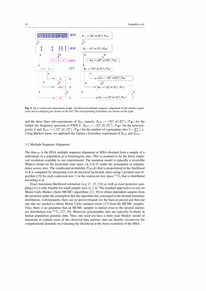
Fig. 4 An n-coalescent experiments graph. An observed multiple sequence alignment of the mother experi-ment and its offspring are shown on the left. The corresponding formalities are shown on the right.

and the three liner sub-experiments of X01, namely, X011 := (Y mn ,σ(Y m

n ),P ΦΦ ) for thefolded site frequency spectrum or FSFS Y , X012 := (Z m

n ,σ(Z mn ),P ΦΦ ) for the heterozy-

gosity Z and X013 := (S mn ,σ(S m

n ),P ΦΦ ) for the number of segregating sites S = ∑n−1i=1 xi.

Using Markov bases, we approach the Tajima’s D product experiment of X012 and X013.

3.1 Multiple Sequence Alignment

The data uo is the DNA multiple sequence alignment or MSA obtained from a sample of nindividuals in a population at m homologous sites. This is assumed to be the finest empir-ical resolution available to our experimenter. The mutation model is typically a reversibleMarkov model on the nucleotide state space {A,C,G,T} under the assumption of indepen-dence across sites. The conditional probability P(uo|φ) that is proportional to the likelihoodof φ is computed by integrating over all ancestral nucleotide states using a product-sum al-gorithm [15] for each coalescent tree ct in the coalescent tree space CnTn that is distributedaccording to φ .

Exact maximum likelihood estimation (e.g. [7, 23, 53]) as well as exact posterior sam-pling [41] is only feasible for small sample sizes (n≤ 4). The standard approach is to rely onMonte Carlo Markov chain (MCMC) algorithms [21, 36] to obtain dependent samples fromthe posterior under the assumption that the algorithm has converged to the desired stationarydistribution. Unfortunately, there are no proven bounds for the burn-in period and thin-outrate that are needed to obtain Monte Carlo standard errors [27] from the MCMC samples.Thus, there is no guarantee that an MCMC sampler is indeed close to the desired station-ary distribution over CnTn [37, 38]. Moreover, polymorphic sites are typically bi-allelic inhuman population genomic data. Thus, one need not have a finite state Markov model ofmutations to explain most of the observed data patterns and can thereby circumvent thecomputational demands on evaluating the likelihood at the finest resolution of the MSA.


3.2 Binary Incidence Matrix

We assume the ancestral nucleotides are known, and at most one derived nucleotide occursat each site among the sampled sequences (such bi-allelic data is common and sites showingancestral and derived characters are commonly referred to as single nucleotide polymor-phisms or SNPs). Then from the aligned sequence data u, we obtain a BIM v ∈ V m

n :={0,1}n×m by replacing all ancestral states with 0 and derived states with 1.

BIM data is modelled by superimposing Watterson’s infinitely-many-sites (IMS) modelof mutation [51] over an n-coalescent sample genealogy [31, 32]. We can conduct inferenceon the basis of the observed binary incidence matrix or BIM v using existing importancesampling methods (e.g. [1, 5, 18, 19, 26, 45, 46]). In this study we are not interested ininference on the basis of the observed BIM at a single locus, but instead on its SFS, a furthersummary of BIM.

3.3 Site Frequency Spectrum

We can obtain the site frequency spectrum x from the BIM v via its site sum spectrum or SSSw. With w denoting the vector of column sums of v, the SFS x is the vector of frequencies ofoccurrences of each positive integer in w. Thus the i-th entry of x records at how many sitesexactly i sequences in u show the derived state. We assume that no site displays only thederived state. Thus, x has only n−1 entries. Figure 5 depicts the BIM v, SSS w and SFS xon the right for a sample of four individuals with the genealogical and mutational history onthe left. Next, we describe the basic probability models required to compute the likelihoodof SFS.

Fig. 5 At most one mutation per site under the infinitely-many-sites model are superimposed as a homoge-neous Poisson process upon the realization of identical coalescent trees at nine homologous SITES labeled{1,2, . . . ,9} that constitute a non-recombining locus from four INDividuals labeled {1,2,3,4}.

16 Sainudiin et al.

3.3.1 Inference under the Unlabeled n-Coalescent

For a given coalescent tree ct ∈ CnTn, let the map:

L(ct) = l := (l1, l2, . . . , ln−1) : CnTn→Ln := Rn−1+ (3.1)

compress the tree ct into the n− 1 lineage lengths that could lead to singleton, doubleton,. . . , and “(n−1)-ton” observations of mutationally derived states, respectively, i.e., li is thelength of all the lineages in ct that subtend i samples or leaves. For example in Fig. 5, (i) thebold lineage of the tree with label set L = {1,2,3,4} upon which the mutations at sites 3 and6 occur, lead to singleton mutations, (ii) the bold-dashed lineage upon which the mutationat site 7 occurs leads to doubleton mutations and (iii) the thin-dashed lineage upon whichmutations at sites 2 and 9 occur lead to tripleton mutations. Thus, l1, l2 and l3 are the lengthsof these three types of lineages, respectively. Finally, l• := ∑

n−1i=1 li ∈R+ is the total length of

all the lineages of the tree ct that are ancestral to the sample since the most recent commonancestor at each one of the m sites at our locus. Now, let li := li/l• be the relative lengthof lineages that subtend i leaves at each site. Now, define l := (l1, l2, . . . , ln−1) ∈ 4n−2, the(n− 2)-unit-simplex containing all l ∈ Rn−1

+ such that ∑n−1i=1 li = 1. Then, if L(ct) = l, the

following conditional probability of x is given by the Poisson-Multinomial distribution:

P(x|φ , ct) = P(x|φ , l) = e−φ1ml•(φ1ml•)s

n−1

∏i=1

lxii /

n−1

∏i=1

xi!, (3.2)

where, s = ∑n−1i=1 xi is the number of segregating sites. The distribution on CnTn is given

by the φ2-indexed n-coalescent approximation of the sample genealogy in an exponentiallygrowing Wright-Fisher model. This distribution on CnTn in turn determines the distribu-tion of the random vector L on Ln. We employ the appropriate lumped Markov process toefficiently obtain P(φ |x) as per Remark 2.

Remark 2 Kemeney & Snell [29, p. 124] observe the following about a lumped process: “Itis also often the case in applications that we are only interested in questions which relate tothis coarser analysis of the possibilities. Thus it is important to be able to determine whetherthe new process can be treated by Markov chain methods.”

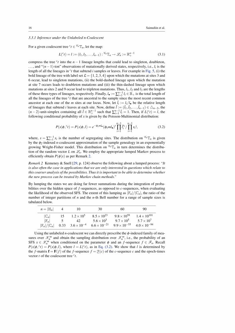
By lumping the states we are doing far fewer summations during the integration of proba-bilities over the hidden space of f -sequences, as opposed to c-sequences, when evaluatingthe likelihood of the observed SFS. The extent of this lumping as |Fn|/|Cn|, the ratio of thenumber of integer partitions of n and the n-th Bell number for a range of sample sizes istabulated below.

n = |Hn| 4 10 30 60 90

|Cn| 15 1.2×105 8.5×1023 9.8×1059 1.4×10101

|Fn| 5 42 5.6×103 9.7×105 5.7×107

|Fn|/|Cn| 0.33 3.6×10−4 6.6×10−21 9.9×10−55 4.0×10−94

Using the unlabeled n-coalescent we can directly prescribe the φ -indexed family of mea-sures over X m

n and obtain the sampling distribution over X mn , i.e., the probability of an

SFS x ∈ X mn when conditioned on the parameter φ and an f -sequence f ∈ Fn. Recall

P(x|φ , ct) = P(x|φ , l), where l = L(ct), as in Eq. (3.2). We show that l is determined bythe f -matrix f = F( f ) of the f -sequence f = F(c) of the c-sequence c and the epoch-timesvector t of the coalescent tree ct.


Proposition 5 (Probability of SFS given f -sequence and epoch-times) Let ct ∈ CnT bea given coalescent tree, c be its c-sequence, f = F(c) be its f -sequence, f = F( f ) be itsf -matrix and t = (t2, t3, . . . , tn) ∈ (0,∞)n−1 be its epoch times as a column vector and itstranspose tT be the corresponding row vector. Then, L(ct) = l of Eq. (3.1) is given by thefollowing matrix multiplications:

l = tTf =

(n

∑i=2

ti fi,1,n−1

∑i=2

ti fi,2, . . .2

∑i=2

ti fi,n−1

). (3.3)

More succinctly, l j = ∑n+1− ji=2 ti fi, j for j = 1,2, . . . ,n− 1. And the probability of an SFS x

given a vector of epoch-times t ∈ (0,∞)n−1 and any coalescent tree ct ∈ F−1( f )t := {ct : c ∈F−1( f )} is:

P(x|φ , ct) = P(x|φ , l) = P(x|φ , tTf

)=

1

∏n−1i=1 xi!

exp

−φ1mn−1

∑j=1

n+1− j

∑i=2

ti fi, j

φ1m

n−1

∑j=1

n+1− j

∑i=2

ti fi, j

∑

n−1i=1 xi

n−1

∏i=1

n+1− j

∑i=2

ti fi, j

n−1

∑j=1

n+1− j

∑i=2

ti fi, j

−1

xi

. (3.4)

Proof The proof of Eq. (3.3) is merely a consequence of the encoding of f as the matrix fand Eq. (3.4) follows from Eqs. (3.3) and (3.2). ut

The computation of l from t and f requires at most n2−2n+1 multiplications and additionsover R. Exploiting the predictable sparseness of f is more efficient especially for large n.Thus, given the parameter φ = (φ1,φ2) and a sample size n, we can efficiently draw SFSsamples from X m

n via Alg. 1.

Algorithm 1 SFS Sampler under Kingman’s unlabeled n-coalescent1: input:

1. scaled mutation rate φ1 per site2. sample size n3. number of sites m at the locus

2: output: an SFS sample x from the standard neutral n-coalescent3: generate an f -sequence f either under {F↑(k)}k∈[n]− or {F↓(k)}k∈[n]+

4: draw t ∼ T = (T2,T3, . . . ,Tn)∼⊗n

i=2( i

2

)e−(

i2)ti , or as desired from Rn−1

+5: draw x from the ( f , t)-dependent Poisson-Multinomial distribution of Eq. (3.4)6: return: x

Note that Alg. 1 is quite general since the only restriction on t in step 4 is that it be apositive real vector. Thus, any indexed family of measures over (0,∞)n−1, including non-parametric ones, may be used provided the c-sequence c and its f -sequence f = F(c) aredrawn from the labeled n-coalescent and the corresponding unlabeled n-coalescent, respec-tively, in an exchangeable manner that is independent of the epoch-times vector t.

Next we study one f -sequence in detail as it is an interesting extreme case that willresurface in the sequel.

18 Sainudiin et al.

Example 3 (completely unbalanced tree) Let the f -sequence fh ∈ Fn denote that of thecompletely unbalanced tree. Its probability based on Eqs. (2.8) and (2.9) are:

fh := ( fh1 , fh2 , . . . , fhn ), where, fhi = (i−1)e1 + e(n−i+1), (3.5)

P( fh) =2

∏i=n

P( fhi−1| fhi ) =2

∏i=n−1

(i−1)1i(i−1)/2

=2n−2

(n−1)!. (3.6)

The number of c-sequences corresponding to it is |F−1( fh)|= n!/2.

The posterior distribution P(φ |x) ∝ P(x|φ)P(φ) over ΦΦ is the object of inferential inter-est. For an efficient inference based on SFS x, we first investigate the topological informationabout the tree ct that the SFS x was realized upon. We are only interested in this informa-tion provided by the drawn x and thus can only resolve the topology of ct up to equivalenceclasses of F−1( f ), where f is the f -sequence corresponding to the c-sequence of ct. Forsamples of size 2 ≤ n ≤ 3 there is only one f -sequence in Fn. For samples with n ≥ 4,consider the following mapping of the SFS x ∈X m

n into vertices of the unit hyper-cube{0,1}n−1, a binary encoding of 2{1,2,...,n−1}, the power set of {1,2, . . . ,n−1}:

X~(x) = x~ := (x~1 , . . . ,x~n−1) := (11N(x1), . . . ,11N(xn−1)) : X mn →{0,1}n−1.

If x~h = 1 then the h-th entry of the SFS x is at least one, i.e., xh > 0. Thus, X~(x) = x~

encodes the presence or absence of at least one site’s ancestral lineage that has been hitby a mutation while subtending h samples, where h ∈ {1,2, . . . ,n− 1}. Next, consider thefollowing two sets of f -sequences:

zn(x~) :=⋃

{h: x~h =1}

{ f ∈Fn :n

∑i=1

fi,h = 0}, {zn(x~) := Fn \zn(x~). (3.7)

The set of f -sequences zn(x~) and its complement {zn(x~) play a fundamental role in in-ference from an SFS x and its X~ = x~. Note that when an SFS x has none of the xi’s equal-ing 0, then its x~ = (1,1, . . . ,1) and {zn(x~) only contains the f -sequence correspondingto the completely unbalanced tree fh given by Eq. (3.5). At the other extreme, when anSFS x has all its xi’s equaling 0 with x~ = (0,0, . . . ,0), we are unable to discriminate amongf -sequences since {zn(x~) = Fn. Thus,

{zn(0,0, . . . ,0) = Fn and {zn(1,1, . . . ,1) = { fh}. (3.8)

Therefore, the size of {zn(x~) can range from 1 to |Fn|, depending on x~. More generally,we have the following Proposition.

Proposition 6 (Likelihood of SFS) For any t ∈ (0,∞)n−1 and any x ∈ X mn with x~ =

X~(x),

If f ∈zn(x~) and l = tT ·F( f ) thenn−1

∏i=1

lxii = 0. (3.9)

Therefore, the likelihood of SFS x is proportional to:

P(x|φ) =1

∏n−1i=1 xi!

∑f∈{zn(x~)

P( f )

∫t∈(0,∞)n−1

exp

−φ1mn−1

∑j=1

n+1− j

∑i=2

ti fi, j

φ1m

n−1

∑j=1

n+1− j

∑i=2

ti fi, j

∑

n−1i=1 xi

n−1

∏i=1

n+1− j

∑i=2

ti fi, j

n−1

∑j=1

n+1− j

∑i=2

ti fi, j

−1

xidP(t|φ)

. (3.10)


Proof We first prove the implication in Eq. (3.9). Given any t ∈ (0,∞)n−1 and any x ∈X mn

with x~ = X~(x), let f ∈ zn(x~). First, suppose x~h = 0 for every h ∈ {1,2, . . . ,n− 1},then zn(x~) = /0 and we have nothing to prove. Now, suppose there exists some h such thatx~h = 1, or equivalently xh > 0, then by the constructive definition of zn(x~), we have thatfor any f ∈zn(x~) ∑

ni=1 fi,h = 0, which implies that fi,h = 0 for every i ∈ {1,2, . . . ,n} since

fi, j ≥ 0. Therefore, by applying this implication to the expression for lh in Prop. 5, we havethat lh = ∑

n+1−hi=2 ti fi,h = 0 and finally the desired equality that ∏

n−1i=1 lxi

i = 0 in Eq. (3.9) is aconsequence of lxh

h = (lh/l•)xh = 0xh = 0.

Next we prove Eq. (3.10). For simplicity, we abuse notation and write P(·) to denote theprobability as well as the probability density under the appropriate dominating measure. Re-peated application of the definition of conditional probability and the neutral structure of then-coalescent model leads to the following expression for P(x,φ) in P(x|φ) = P(x,φ)/P(φ).

P(x,φ) = ∑c∈Cn

∫t∈(0,∞)n−1

P(x,φ , t,c) = ∑f∈Fn

∫t∈(0,∞)n−1

P(x,φ , t, f )

= ∑f∈Fn

∫t∈(0,∞)n−1

P(x|φ , t, f )P(φ , t, f )

= ∑f∈Fn

P( f )∫

t∈(0,∞)n−1P(x|φ , l = tT ·F( f )

)P(t|φ)P(φ)

since, by independence of f and (φ , t)

P(φ , t, f ) = P( f |φ , t)P(φ , t) = P( f )P(φ , t) = P( f )P(t|φ)P(φ).

Thus, by letting F( f ) = f, the likelihood of the SFS x is:

P(x|φ) = P(x,φ)/P(φ) = ∑f∈Fn

P( f )∫

t∈(0,∞)n−1P(x|φ , l = tT · f

)dP(t|φ).

Substituting for P(x|φ , l = tT · f) from Prop. 5 and only summing over f ∈ {zn(x~) withnon-zero probability P(x|φ , l = tT · f), we get the discrete sum weighted by integrals on Tn :=(0,∞)n−1, the required equality in Eq. (3.10). ut

Next we devise an algorithm to estimate P(x|φ), the probability of an observed SFS xgiven a parameter φ . This is accomplished by constructing a Markov chain {F�x~(k)}k∈[n]+

on the state space Fx~n ⊂ Fn×{0,1}n−1 such that every sequence of states visited by this

chain yields a probable f -sequences f for the observed SFS x, i.e., f ∈ {zn(x~). In thispaper, we focus on small n ∈ {4,5, . . . ,10} and exhaustively sum over all f ∈ {zn(x~)that are unique sequential realizations of {F�x~(k)}k∈[n]+ . The maximal number of suchf -sequences is:

maxx~∈{0,1}n−1

∣∣{zn(x~)∣∣= ∣∣{zn((0,0, . . . ,0))

∣∣= |Fn| .

A breadth-first search on the transition graph of {F�x~(k)}k∈[n]+ revealed that

|Fn|= 2,4,11,33,116,435,1832, . . . ,6237505, as n = 4,5,6,7,8,9,10, . . . ,15,

respectively. Our computations are in agreement with similar numerical calculations of |Fn|in [10, Sec. 2]. This x~-indexed family of 2n−1 Markov chains {F�x~(k)}k∈[n]+ over state

20 Sainudiin et al.

((0 0 0 0 1),(* * 0 0))

((1 0 0 1 0),(* * 0 0))

1/2

((0 1 1 0 0),(* * 0 0))

1/2

((2 0 1 0 0),(* * 0 0))

2/3

((1 2 0 0 0),(* * 0 0))

1/31/3 2/3

((3 1 0 0 0),(* * 0 0))

1 1

((5 0 0 0 0),(* * 0 0))

1

((0 0 0 0 1),(* * 0 1))

1

((0 0 0 0 1),(* * 1 0))

1/2

((1 0 0 1 0),(* * 1 0))

1/2

1

((0 0 0 0 1),(* * 1 1))

1

Fig. 6 Transition diagram of {F�x~ (k)}k∈[5]+ over states in Fx~n . The simplified diagram replaces the states

that do not affect the transitions, namely, x~1 and x~2 , with ∗ ∈ {0,1}.

spaces contained in Fn×{0,1}n−1 may also be thought of as a controlled Markov chain(e.g. [9, §7.3]) over the state space Fn with control space {0,1}n−1 that can produce thedesired f -sequences in {zn(x~).

Optimal importance sampling by using the sequential realizations of {F�x~(k)}k∈[n]+and its continuous time variant as a proposal distribution in order to get the Monte Carloestimate of P(x|φ) for larger n is necessary and possible. However, this is a subsequentproblem in variance reduction of the Monte Carlo estimate for large values of n that dependsfurther on the precise nature of φ -indexed measures on CnTn.

Proposition 7 (A Proposal over {zn(x~)) For a given SFS x ∈X mn and X~(x) = x~ ∈

{0,1}n−1, consider the discrete time Markov chain {F�x~(k)}k∈[n]+ over the state spaceof ordered pairs ( fi′ ,zi′) ∈ Fx~

n ⊂ Fn×{0,1}n−1, with the initial state given by ( f1,x~) =((0,0, . . . ,1),x~), the transition probabilities obtained by a controlled reweighing of thetransition probabilities of {F↓(k)}k∈[n]+ over Fn as follows:

P(( fi′ ,zi′)|( fi,zi)) =

{P( fi′ | fi)/Σ( fi,zi) : if ( fi,zi)≺ f ,z ( fi′ ,zi′),0 : otherwise,

(3.11)

where,Σ( fi,zi) = ∑

( j,k)∈Ξ( fi,zi)P( fi− e j+k + e j + ek| fi),

Ξ( fi,zi) :={( j,k) : fi, j+k > 0, 1≤ j ≤ j ≤ k ≤ j + k−1

},

j := max{

min{

max{` : zi,` = 1}, j + k−1}

,

⌈j + k

2

⌉},


( fi,zi)≺ f ,z ( fi′ ,zi′) ⇐⇒

{fi′ = fi + e j + ek− e j+k,( j,k) ∈ Ξ( fi,zi), andzi′ = zi−11{1}(zi, j)e j−11{1}(zi,k)ek,

and with ( fn,(0,0, . . . ,0)) = ((n,0, . . . ,0),(0,0, . . . ,0)) as the final absorbing state.Let F x~

n be the set of sequential realizations of the first component of the ordered pairsof states visited by {F�x~(k)}k∈[n]+ , i.e.

F x~n := { f = ( fn, fn−1, . . . , f1) : fi ∈ F(i)

n ,( fi,zi)≺ f ,z ( fi+1,zi+1),z1 = x~}.

Then F x~n = {zn(x~).

Proof We will prove that F x~n = {zn(x~) for three cases after noting that the ortho-normal

basis vector ei in {0,1}n−1 and Fn takes the appropriate dimension. The first two casesinvolve constructive proofs.

Case 1: Suppose x~ = (0,0, . . . ,0). Since {zn(x~) = Fn by Eq. (3.8), we need to showthat F x~

n = Fn. Initially, at time step 1,

F�x~(1) = ( f1,z1) = ( f1,x~) = ((0,0, . . . ,0,1),(0,0, . . . ,0))

Note that for any time step i, zi in the current state ( fi,zi) remains at (0,0, . . . ,0). Thus,max{` : zi,` = 1}= max{ /0}=−∞ and therefore,

j := max{

min{

max{` : zi,` = 1}, j + k−1}

,

⌈j + k

2

⌉}=⌈

j + k2

⌉, and

Ξ( fi,zi) :={

( j,k) : fi, j+k > 0, 1≤ j ≤⌈

j + k2

⌉≤ k ≤ j + k−1

}.

Therefore, the first component of the chain can reach all states in Fn that are immediatelypreceded by fi under≺ f making Σ( fi,zi) = 1. Thus, when x~ = (0,0, . . . ,0) our fully uncon-trolled Markov chain {F�x~(k)}k∈[n]+ visits states in Fn in a manner identical to the Markovchain {F↓(k)}k∈[n]+ over Fn. Therefore, F x~

n = Fn = {zn(x~) when x~ = (0,0, . . . ,0).Case 2: Suppose x~ = (1,1, . . . ,1). Since {zn(x~) = { fh} by Eq. (3.8), we need to

show that F x~n = { fh}. Initially, at time step 1,

F�x~(1) = ( f1,z1) = ( f1,x~) = ((0,0, . . . ,0,1),(1,1, . . . ,1,1))

then fi, j+k > 0 =⇒ j + k = n, max{` : z1,` = 1} = max{1,2, . . . ,n−1} = n− 1, j =max{min{n−1,n−1},dn/2e}= n−1 and

Ξ( f1,z1) ={( j,k) : fi, j+k > 0, 1≤ j ≤ n−1≤ k ≤ n−1}= {(1,n−1)

}.

Thus, the only state that is immediately preceded by ( f1,z1) is our next state ( f2,z2) = ( f1−en + e1 + en−1,z1−11{1}(z1,1)e1−11{1}(zi,n−1)en−1) with probability 1 due to the equality ofthe numerator and denominator in Eq. (3.11):

( f1,z1)≺ f ,z ( f2,z2) = ((1,0, . . . ,1,0),(0,1, . . . ,1,0)) = F�x~(2)

In general, at time step i, Ξ( fi,zi) = {(1,n− i)}, P(( fi+1,zi+1)|( fi,zi)) = 1 and

fi+1 = f1−n

∑j=1

e j +i

∑j=1

e1 +i

∑j=1

en− j = en−i + ie1, zi+1 = x~− e1−n

∑j=i

e j−1.

22 Sainudiin et al.

By Eq. (3.5), fi+1 = en−i + ie1 = fhi+1 and we get the desired fh = ( fhn , fhn−1, . . . , fh1 ) inthe forward direction as the only realization over Fn of our fully controlled Markov chain{F�x~(k)}k∈[n]+ . Therefore, F x~

n = { fh}= {zn(x~) when x~ = (1,1, . . . ,1).Case 3: Now, suppose x~ ∈ {0,1}n−1 \ {(0,0, . . . ,0),(1,1, . . . ,1)}. First, we will show

that f ∈F x~n implies that f ∈ {zn(x~) or equivalently that f /∈ zn(x~). We will prove by

contradiction. Assume f ∈F x~n . Suppose that f ∈zn(x~). Then by Eq. (3.7), there exists an

h with x~h = 1 such that ∑ni=1 fi,h = 0. Since ∑

ni=1 fi,1 > 0 and ∑

ni=1 fi,2 > 0 for every f ∈Fn,

with n > 2, h ∈ {3,4, . . . ,n− 1}. Recall that ∑ni=1 fi,h = 0 implies that there was never a

split of any lineage that birthed a child lineage subtending h leaves at any time step in thesequential realization of f = ( f1, f2, . . . , fn) over Fn by {F�x~(k)}[n]+ . This contradicts ourassumption that f ∈F x~

n as it violates the constrained splitting imposed by Ξ( fi,zi) at thetime step i when max{` : zi,` = 1} = h in the definition of j. So, our supposition that f ∈zn(x~) is false. Therefore, if f ∈F x~

n then f ∈ {zn(x~). Next, we will show f ∈ {zn(x~)implies that f ∈F x~

n . Assume that f ∈ {zn(x~), then ∑ni=1 fi,h > 0 for every h∈{h : x~h = 1}

by Eq. (3.7). This means that for each h with x~h = 1 there is at least one split in f that birtheda child lineage subtending h leaves. Since this splitting condition satisfies the constraintsimposed by Ξ( fi,zi) at each time step i when max{` : zi,` = 1} = h, h ∈ {h : x~h = 1}, inthe definition of j, this f can be sequentially realized over Fn by {F�x~(k)}[n]+ . Therefore,if f ∈ {zn(x~) then f ∈F x~

n . ut

Thus, given φ1 and an x~, we can efficiently propose SFS samples from X mn , such that

the underlying f -sequence f belongs to {zn(x~), using Alg. 2. Note however that a furtherstraightforward importance sampling step using Eqs. (3.11) and (2.11) is needed to obtainSFS samples that are distributed over X m

n according to the unlabeled n-coalescent over{zn(x~).

Algorithm 2 SFS Proposal under an x~-controlled unlabeled n-coalescent1: input:

1. scaled mutation rate φ1 per site2. number of sites m at the locus3. observed x~ (note that sample size n = |x~|+1)

2: output: an SFS sample x such that the underlying f -sequence f ∈ {zn(x~)3: generate an f -sequence f under {F�x~ (k)}k∈[n]+

4: draw t ∼ T = (T2,T3, . . . ,Tn)∼⊗n

i=2( i

2

)e−(

i2)ti , or as desired from Rn−1

+5: draw x from the ( f , t)-dependent Poisson-Multinomial distribution of Eq. (3.4)6: return: x

3.4 Linear experiments of the site frequency spectrum

We describe a method to obtain the conditional probability P(r|φ , ct), where r = Rx is a setof classical population genetic statistics that are linear combinations of the site frequencyspectrum x, φ is the vector of parameters in the population genetic model and ct is theunderlying coalescent tree upon which mutations are superimposed to obtain the data. Theconditional probability is obtained by an appropriate integration over

R−1(r) := {x : x ∈ Zn−1+ ,Rx = r}.


R−1(r) is called a fiber.We want to compute P(r|φ), since the posterior distribution of interest is P(φ |r) ∝

P(r|φ)P(φ). Furthermore, we assume a uniform prior over a biologically sensible grid ofφ values and evaluate P(r|φ) over each φ in our grid. More precisely, we have:

P(r|φ , ct) = P(r|φ , l = L(ct)) = ∑x∈R−1(r)

P(x|φ , l), (3.12)

P(r|φ) =∫

l∈Ln

P(r|φ , l)P(l|φ) =∫

l∈Ln∑

x∈R−1(r)

P(x|φ , l)P(l|φ). (3.13)

We can approximate the two integrals in Eq. (3.13) by the finite Monte Carlo sums,

P(r|φ)≈ 1N

N

∑j=1

1M

M

∑h=1,

x(h)∈R−1(r)

P(x(h)|φ , l( j)), l( j) ∼ P(l|φ). (3.14)

The inner Monte Carlo sum approximates ∑x P(x|φ , l) over M x(h)‘s in R−1(r) and the outerMonte Carlo sum over N different l( j)‘s can be obtained from simulation under φ . Therefore,P(φ |r) ∝ P(r|φ)P(φ)

≈ 1N

N

∑j=1

1M

M

∑h=1,

x(h)∈R−1(r)

P(x(h)|φ , l( j)), l( j) ∼ P(l|φ)P(φ).

If |R−1| is not too large, say less than a million, then we can do the inner summation exactlyby a breadth-first traversal of an implicit graph representation of R−1(r). In general, the sumover R−1(r) is accomplished by a Monte Carlo Markov chain on a graph representationof the state space R−1(r) that guarantees irreducibility. This article is mainly concernedwith the application of Markov bases to facilitate these integrations over R−1(r). AlthoughMarkov bases were first introduced in the context of exact tests for contingency tables [8],we show in this article that they can also be used to obtain the posterior distribution P(φ |ro)of various observed population genetic statistics ro.

Definition 1 (Markov Basis) Let R be a q× (n− 1) integral matrix. Let MR be a finitesubset of the intersection of the kernel of R and Zn−1. Consider the undirected graph G r

R,such that (1) the nodes are all lattice points in R−1(r) and (2) edges between a node x anda node y are present if and only if x− y ∈MR. If G r

R is connected for all r with G rR 6=

/0, then MR is called a Markov basis associated with the matrix R. We refer to an m :=(m1, . . . ,m(n−1)) ∈MR as a move.

A Markov basis can be computed with computational commutative algebraic algorithms[8] implemented in algebraic software packages such as Macaulay 2 [17] and 4ti2 [22].Monte Carlo Markov chains constructed with moves from MR are irreducible and can bemade aperiodic, and are therefore ergodic on the finite state space R−1(r). An ergodicMarkov chain is essential to sample from some target distribution on R−1(r) using MonteCarlo Markov chain (MCMC) methods.

24 Sainudiin et al.

3.4.1 Number of Segregating Sites

A classical statistic in population genetics is S, the number of segregating sites [51]. It canbe expressed as the sum of the components of the SFS x:

S(x) :=n−1

∑i=1

xi = s : X mn →S m

n . (3.15)

S is the statistic of the n-coalescent experiment X013 := (S mn ,σ(S m

n ),P ΦΦ ). For somefixed sample size n at m homologous and at most bi-allelic sites, let the s-simplex S−1(s) ={x ∈X m

n : S(x) = s} denote the set of SFS that have the same number of segregating sites s.The size of S−1(s) is given by the number of compositions of s by n−1 parts, i.e., |S−1(s)|=(s+n−2

s

). The conditional probability of S is Poisson distributed with rate parameter given by

the product of the total tree size l• := ∑n−1i=1 li, number of sites m and the per-site scaled

mutation rate parameter φ1 in φ

P(S = s|φ , ct) = P(S = s|φ , l) = ∑x∈S−1(s)

P(x|φ , l)

= ∑x∈S−1(s)

e−φ1ml•(φ1ml•)s

n−1

∏i=1

lxii

(n−1

∏i=1

xi!

)−1

= e−φ1ml•(φ1ml•)s/s!

3.4.2 Heterozygosity

Another classical summary statistic called average heterozygosity is also a symmetric lin-ear combination of SFS x [47]. We define heterozygosity Z(x) = z and average pair-wiseheterozygosity Π(x) = π for the entire locus as follows:

Z(x) :=n−1

∑i=1

i(n− i)xi, Π(x) :=1(n2

)Z(x). (3.16)

Z is the statistic of the n-coalescent experiment X012 := (Z mn ,σ(Z m

n ),P ΦΦ ). For somefixed sample size n at m homologous and at most biallelic sites, consider the set of SFS thathave the same heterozygosity z denoted by Z−1(z) = {x∈X m

n : Z(x) = z}. This set is the in-tersection of a hyper-plane with X m

n . The conditional probability P(Z|φ , ct) = P(Π |φ , ct) =P(Z = z|φ , l) is

P(Z = z|φ , l) = ∑x∈Z−1(z)

P(x|φ , l) = e−φ1ml• ∑x∈Z−1(z)

(φ1ml•)∑n−1i=1 xi ∏

n−1i=1 lxi

i

∏n−1i=1 xi!

.

3.4.3 Tajima’s D

Tajima’s D statistic [47] for a locus only depends on the number of segregating sites ofEq. (3.15), average pair-wise heterozygosity of Eq. (3.16) and the sample size n, as follows:

D(x) :=Π(x)−S(x)/d1√

d3S(x)+d4S(x)(S(x)−1), (3.17)


where, d1 := ∑n−1i=1 i−1, d2 := ∑

n−1i=1 i−2,

d3 :=n+1

3d1(n−1)− 1

d21, d4 :=

1d2

1 +d2

(2(n2 +n+3)

9n(n−1)− n+2

nd1+

d2

d21

).

Thus, Tajima’s D is a statistic of X012×X013, a product n-coalescent experiment. Let r =(s,z)′ for a given sample size n. Observe that fixing n and r also fixes the average heterozy-gosity π and Tajima’s d. Next we will see that inference based on s, π and d for a fixedsample size n depends on the kernel or null space of the matrix R given by:

R :=(

1 . . . 1 . . . 11(n−1) . . . i(n− i) . . . (n−1)(n− (n−1))

).

The space of all possible SFS x for a given sample size n is the non-negative integer latticeZn−1

+ . Let the intersection of {x : Rx = r} with Zn−1+ be the set:

R−1(r) :={

x ∈ Zn−1+ : Rx = r

}.

Since n is fixed, every SFS x in R−1(r) has the same s, z, π and d.

Fig. 7 A: Polytopes containing R−1((s,z)′), where z ∈ {30,31, . . . ,40}, n = 4 and s = 10 are at the in-tersection of the s-simplex, Z3

+ and each of the z-simplexes. B: Projected rectangular polytopes containingR−1((s,z)′), where z ∈ {20,22, . . . ,30}, n = 5 and s = 5 (see text).

When n = 4 we can visualize any SFS x∈R−1(r) using Cartesian coordinates. Let R1 =(1,1,1) and R1

−1(s) := {x ∈ Z3+ : ∑

3i=1 xi = s}, the set of SFS with s segregating sites, be

formed by the intersection of Z3+ with the the s-simplex given by x3 = s−x1−x2. Figure 7 A

shows R1−1(10), the set of 66 SFS with 10 segregating sites, as colored balls embedded in

the orange s-simplex with s = 10. Similarly, with R2 = (3,4,3), R2−1(z) := {x ∈Z3

+ : 3x1 +4x2 + 3x3 = z} is the set of SFS at the intersection of Z3

+ with the z-simplex given by x3 =(z−3x1−4x2)/3. Figure 7 A shows three z-simplexes for z = 30,35 and 40, in hues of violet,turquoise and yellow, respectively. Finally, the intersection of a z-simplex, s-simplex and Z3

+is our polytope R−1((s,z)′), the set of SFS that lie along the line (x1,z−3s,−z+4s−x1). InFig. 7 A, as z ranges over {30,31, . . . ,40}, (1) the z-specific hue of the set of balls depicting

26 Sainudiin et al.

the set R−1((10,z)′) ranges over {violet,blue, . . . ,yellow}, (2) |R−1((10,z)′)| ranges over{11,10, . . . ,1} and (3) Tajima’s d ranges over {−0.83,−0.53, . . . ,+2.22}, respectively. Forexample, there are eleven SFS in R−1((10,30)′) and their Tajima’s d =−0.83 (purple ballsin Fig. 7 A) and there is only one SFS in R−1((10,40)′) = {(0,10,0)} such that its Tajima’sd = +2.22 (yellow ball in Fig. 7 A).

Analogously, when n = 5, we can project the first three coordinates of x, since x4 = s−x1− x2− x3. The intersection of the s-simplex, z-simplex and Z4

+ gives our set R−1((s,z)′)in the rectangular polytope via the parametric equation (x1,x2,z/2−2s− x2,3s− z/2− x1)with 0≤ x1 ≤ 3s− z/2, 0≤ x2 ≤ s. In Fig. 7 B, as z ranges over {20,22,24,26,28,30}, (1)the z-specific hue of the set of balls depicting the set R−1((5,z)′) in the projected polytoperanges over {violet,blue, . . . ,yellow}, (2) |R−1((5,z)′)| ranges over {6,10,12,12,10,6} and(3) Tajima’s d ranges over {−1.12,−0.56,0.00,+0.56,+1.69}, respectively.

Unfortunately, |R−1((s,z)′)| grows exponentially with n and for any fixed n it growsgeometrically with s. Thus, it becomes impractical to explicitly obtain R−1(r) for reason-able sample sizes (n > 10). For small sample sizes we used Barvinok’s cone decompositionalgorithm [2] as implemented in the software package LattE [34] to obtain |R−1((s,z)′)|for 1000 data sets simulated under the standard neutral n-coalescent [25] with the scaledmutation rate φ ∗1 = 10. As n ranged in {4,5, . . . ,10}, the maximum of |R−1((s,z)′)| over the1000 simulated data sets of sample size n ranged in:

{73,940,6178,333732,1790354,62103612,190176626},

respectively. Thus, even for samples of size 10, there can be more than 190 million SFS withexactly the same s and z. The SFS data in this simulation study with φ ∗1 = 10 corresponds toan admittedly long stretch of non-recombining DNA sites. On the basis of average per-sitemutation rate in humans, this amounts to simulating human SFS data from n individualsat a non-recombining locus that is 100kbp long, i.e., m = 105. Although such a large mis atypical for most non-recombining loci, it does provide a good upper bound for m andcomputational methods developed under a good upper bound are more likely to be efficientfor smaller m. Our choices of φ ∗1 and m are biologically motivated by a previous study onhuman SNP density [42].

Thus |R−1((s,z)′)| can make explicit computations over R−1(r) impractical, especiallyfor larger n. However, there are two facts in our favor: (1) if we are only interested in anexpectation over R−1(r) (with respect to some concentrated density) for reasonably sizedsamples (e.g. 4 ≤ n ≤ 120), then we may use a Markov basis of R−1(r) to facilitate MonteCarlo integration over R−1(r) and (2) for specific summaries of SFS, such as the folded SFSy := (y1,y2, . . . ,ybn/2c), where y j := 11{ j 6=n− j}( j) x j +xn− j, one can specify the Markov basisfor any n.

The number of moves |MR| ranged over {2,4,6,8,14,12,26,520,10132} as n rangedover {4,5, . . . ,9,10,30,90}, respectively. The Markov basis for R−1(r) when n = 4 is MR ={(+1,0,−1),(−1,0,+1)}. From the example of Fig. 7 A we can see how R−1(r) can beturned into a connected graph by MR for every r with S = 10. For instance, when r =(10,36)′,

R−1(r) = {(0,6,4),(1,6,3),(2,6,2),(3,6,1),(4,6,0)}

and we can reach a neighboring SFS x ∈ R−1(r) from any SFS x ∈ R−1(r) by adding(+1,0,−1) or (−1,0,+1) to x, provided the sum is non-negative. When the sample sizen = 5, a Markov basis for R−1(r) is

MR = {(+1,0,0,−1),(−1,0,0,+1),(0,+1,−1,0),(0,−1,+1,0)}


and once again we can see from Fig. 7 B that any element m ∈MR can be added to anyx ∈R−1(r), for any r, to reach a neighbor within R−1(r), proviso quod, xi +mi ≥ 0,∀i. Notethat the maximum possible neighbors of any x ∈ R−1(r) is bounded from above by |MR|.

3.4.4 Folded Site Frequency Spectrum

The folded site frequency spectrum or FSFS y := (y1,y2, . . . ,ybn/2c) is essentially the SFSwhen one does not know the ancestral state of the nucleotide. It is determined by the mapY (x) = y : X m

n → Y mn :

Y (x) := (Y1(x),Y2(x), . . . ,Ybn/2c(x)),

Yj(x) := x j11{ j 6=n− j}( j)+ xn− j, j ∈ {1,2, . . . ,bn/2c} (3.18)

Y is the statistic of the n-coalescent experiment X011 := (Y mn ,σ(Y m

n ),P ΦΦ ). The caseof the FSFS y is particularly interesting since a Markov basis is known for any sample sizen. Let ei be the i-th unit vector in Zn−1. A Markov basis of the set of y-preserving SFSY−1(y) := {x : Yx = y} can be obtained by considering the null space of the matrix Y,whose i-th row Yi is:

Yi = 11{ j: j 6=(n− j)}(i) ei + en−i, i = 1,2, . . . ,bn/2c.

A minimal Markov basis MY for Y−1(y) is known explicitly for any n and contains theunion of the following 2bn/2c moves only:{

mi = ei− en−i, i = 1,2, . . . ,bn/2c,mn−i =−ei + en−i, i = 1,2, . . . ,bn/2c.

The following algorithm can be used to make irreducible random walks in Y−1(y): (i)Given an SFS x with folded SFS y, (ii) Uniformly pick j ∈ {1,2, . . . ,b(n− 1)/2c}, (iii)Uniformly pick k ∈ { j,n− j}, (iv) Add +1 to xk and add−1 to x(n−k), provided x(n−k)−1≥0, to obtain an y-preserving SFS x from x.

Note that x and x have the same folded SFS y and fixing y also fixes s, z, Tajima’s d andother summaries that are symmetric linear combinations of the SFS x. Thus, MY ⊆MR.For instance, when n = 3, MY = MR = {(−1,+1),(+1,−1)} and we have already seenthat MY = MR when n = 4,5. However, when n ≥ 6 we may not necessarily have suchan equality, i.e., MY ( MR. When n = 6 our MR has extra moves so that MR \MY ={(+1,−4,+3,+0,+0),(−1,+4,−3,+0,+0)}. The size of the set Y−1(y) follows from abasic permutation argument as:

|Y−1(y)|=b n−1

2 c∏i=1

(yi +1).

3.4.5 Other Linear Experiments of the Site Frequency Spectrum

In principle, we can compute a Markov basis for any conditional lattice G−1(g), such thatGx = g∈Zk, for some k×(n−1) matrix G := (gi, j),gi, j ∈Z+. Specifically, it is straightfor-ward to add other popular summaries of the SFS. Examples of such linear summaries rangefrom the unfolded singletons x1, folded singletons y1 := x1 + x(n−1) [24] and Fay and Wu’sθH := (n(n−1))−1

∑n−1i=1 (2 i2 xi) [14].

28 Sainudiin et al.

3.4.6 Integrating over Neighborhoods of Site Frequency Spectra

Recall that a Markov basis MR for an observed linear summary ro of the observed SFS xomay be used to integrate some target distribution of interest over the set R−1(ro) := {x ∈Zn−1

+ : Rx = ro}. Such an integration may be conducted deterministically or stochastically. Asimple deterministic strategy may entail a depth-first or a breadth-first search on the graphG ro

R associated with the set R−1(ro) after initialization at xo. A simple stochastic strategymay entail the use of moves in MR as local proposals for a Monte Carlo Markov chainsampler (MCMC) that is provably irreducible on R−1(ro). Such an MCMC sampler can beconstructed, via the Metropolis-Hastings kernel for instance, to asymptotically target anydistribution over the set R−1(ro) := {x ∈ Zn−1

+ : Rx = ro}. Since every SFS state visitedby such an MCMC sampler is guaranteed to exactly satisfy ro, provided the algorithm isinitialized at the observed SFS xo and quickly converges to stationarity, one may hope tovanish the acceptance-radius ε altogether in practical approximate Bayesian computationsthat employ linear summaries of the SFS. One may use standard algebraic packages to com-pute MR for reasonably large sample sizes (n < 200). Furthermore, for perfectly symmetricsummaries such as the folded SFS y we know a Markov basis for any n.

Unfortunately, the methodology is not immune to the curse of dimensionality. The set’scardinality (|R−1((s,z)′)|) grows exponentially with n and for any fixed n it grows geo-metrically with the number of segregating sites s. This makes exhaustive integration of atarget distribution over R−1(ro) impractical even for samples of size 10 with a large num-ber of segregating sites. Also, even if we were to approximate the integral via Monte CarloMarkov chain with local proposals from the moves in MR, the number of possible neigh-bors for some points in R−1(ro) may be as high as |MR|. For instance, when the sample sizen = 90, we may have up to 10132 moves. Such large degrees can lead to poor mixing of theMCMC sampler, especially when the initial condition is at the tail of the target distribution.However, there are some blessings that counter these curses. Firstly, the concentration of thetarget distribution under the n-coalescent greatly reduces the effective support on R−1(ro).Secondly, we can be formally interpolative in our integration strategy by exploiting the graphG ro

R associated with the set R−1(ro) and the observed SFS xo. Instead of integrating a targetdistribution over all of R−1(ro), either deterministically or stochastically, we can integrateover a ball of edge radius α about the observed SFS xo:

R−1α (ro) := {x ∈ Zn−1

+ : Rx = ro, ||x− xo|| ≤ α},

where, ||x− xo|| is the minimum number of edges between an SFS x and the observed SFSxo. This integration over R−1

α (ro) may be conducted deterministically via a simple breadth-first search on the graph G ro

R associated with the set R−1(ro) by initializing at xo. When adeterministic breadth-first search becomes inefficient, especially for large values of α , onemay supplement with a Monte Carlo sampler that targets the distribution of interest overR−1

α (ro). Since R−10 (ro) = {xo} and R−1

∞ (ro) = R−1(ro), one can think of R−1α (ro) itself

as an α-family of summary statistics that interpolates between the observed SFS xo at oneextreme and the observed coarser summary ro at the other. For a given observation xo with itscorresponding ro and some reasonably large values of α , we can obtain R−1

α (ro) independentof the target distribution via a single depth-first search. This is more efficient than a target-specific Monte Carlo integration over R−1

α (ro) when we want to integrate multiple targets.Thus, we can integrate any target or set of targets over R−1

α (ro) and thereby measure theextent of posterior concentration as α decreases from ∞ at one extreme to 0 at the other.


3.4.7 A Demographic Structured Population

Next we demonstrate the generality of the methodology by studying a more complex modelthrough linear summaries of more general summaries of the full data. For example, considerdata from two known sub-populations A and B with sample sizes nA and nB, respectively,such that n = nA +nB. We can first summarize the data do into three vectors xA, xB and xAB

that can be thought of as a decomposition of the SFS based on sub-populations. Unlike thefull SFS x ∈ Zn−1

+ ,xA := (xA

1 , . . . ,xAnA) ∈ ZnA

+ ,

xB := (xB1 , . . . ,xB

nB) ∈ ZnB+ ,

xAB := (xAB2 , . . . ,xAB

n−1) ∈ Zn−2+ ,

where, xJi is the number of sites that have i samples only from sub-population J ∈ {A,B}

sharing a mutation (there are no mutations at these sites in the other sub-population). Wecan think of xA and xB as sub-population specific SFS and xAB as the shared SFS. Thus, xAB

iis the number of sites with a total of i samples (at least one sample from each population)having a mutation. Observe that the full SFS x for the entire sample can be recovered fromthe sub-population determined components as follows:

x1 = xA1 + xB

1 ,x2 = xA2 + xB

2 + xAB2 , . . . ,xi = xA

i + xBi + xAB

i , . . . ,xn−1 = xABn−1.

Now, let SA, SB and SAB be the number of segregating sites for A-specific, B-specific andshared SFS, i.e.,

SA :=nA

∑i=1

xAi , SB :=

nB

∑i=1

xBi , and SAB :=

n−1

∑i=2

xABi .

Note that the total number of segregating sites is

S =n−1

∑i=1

xi = SA +SB +SAB.

We are interested in the sub-population determined SFS x given by,

x := (xA,xB,xAB) = (xA1 , . . . ,xA

nA ,xB1 , . . . ,xB

nB ,xAB2 , . . . ,xAB

n−1) ∈ Z2n−2+ .

We refer to x as the structured SFS (SSFS).Let the non-averaged pair-wise heterozygosity be z for the entire sample and be zA and

zB for sites segregating only within sub-population A and B, respectively, i.e.

zA :=nA−1

∑i=1

i(nA− i)xAi , and zB :=

nB−1

∑i=1

i(nB− i)xBi .

Thus, the matrix R encoding the summary r = (SA,SB,SAB,zA,zB,z) is:

R :=

1 . . . 1 0 . . . 0 0 . . . 00 . . . 0 1 . . . 1 0 . . . 00 . . . 0 0 . . . 0 1 . . . 1

1(nA−1) . . . 0 0 . . . 0 0 . . . 00 . . . 0 1(nB−1) . . . 0 0 . . . 0

1(n−1) . . . nA(n−nA) 1(n−1) . . . nB(n−nB) 2(n−2) . . . n−1

.

Observe that Tajima’s D for the entire sample as well as the sub-population specific DA

and DB computed from the sites that are segregating only within sub-population A and B,

30 Sainudiin et al.

respectively, are also constrained by the six summaries. We could naturally add other linearsummaries of x, xA, xB and xAB.

Finally, we can compute a Markov basis for R and use it to run Monte Carlo Markovchains on R−1(r) = {x : Rx = r}. The final ingredient we need is the target distribution onR−1(r) when given some structured n-coalescent tree ct simulated according to φ , i.e., weneed the probability P(x|ct). This is also a Poisson multinomial distribution analogous tothe simpler case with the sample SFS. However, the compression is not as simple as thetotal tree length (l•) and the relative time leading to singletons, doubletons, . . . , “n−1-tons”(l ∈4n−2). Now, we need to divide the total length l• of the tree ct into the length of lineagesleading to mutations in sub-population A alone (lA

• ), in sub-population B alone (lB• ) and those

leading to mutations in both sub-populations (lAB• ). Note that l• = lA

• + lB• + lAB

• . The productsof these three lengths lA

• , lB• and lAB

• with φ1 specifies the Poisson probability of observingSA, SB and SAB, respectively. To get the multinomial probabilities of xA, xB and xAB, wedo a sub-population-labeled compression of the structured n-coalescent tree ct into pointsin three simplexes. First, we label all the lineages of ct leading exclusively to mutations insub-population A. Next we compress these labeled lineages into the relative time leading tosingletons, doubletons, . . . , “nA-tons” exclusively within sub-population A. These labeledrelative times yield l

A ∈4nA−1. By an analogous labeling and compression of ct we obtain

lB ∈ 4nB−1. Finally, we obtain the probabilities l

AB ∈ 4n−3 by labeling the lineages on ctthat lead to both sub-populations.

3.5 n-Coalescent Experiments Graph

Having defined each one of the n-coalescent experiments, we next define a graph of n-coalescent experiments. This experiments graph sets a unified decision-theoretic stage thatallows one to appreciate the different asymptotic senses and the partially ordered graph ofsub-σ -algebras or graph filtrations that underlie these classical experiments in populationgenetics.

Definition 2 (The Experiments Graph) Consider {Xα , α ∈ A}, an A-indexed set of ex-periments. Let, Tα,β : Zα → Zβ , for some α,β ∈ A with σ(Zα) ⊃ σ(Zβ ) be a statistic(measurable map). Let M be a set of such maps as well as the identity map. Then, thedirected graph of experiments GA,M with nodes {Xα , α ∈ A} and directed edges from anode Xα to a node Xβ , provided there exists an Tα,β ∈M, is the experiments graph. Con-sider the partial ordering �X induced on the experiments in {Xα , α ∈ A} by the maps inM, i.e., Xα �X Xβ if and only if there exists a composition of maps from M given byT ◦

α,β := Tα,i ◦ Ti, j ◦ · · · ◦ Ti′, j′Tj′,β : Zα → Zβ , such that σ(Zα) ⊃ σ(Zβ ). Then, by con-struction, (i) the random variables {Xα ,α ∈ A} that are adapted to this partially orderedfiltration, i.e., for each α ∈ A, Xα is σ(Xα)-measurable, such that (ii) E(|Xα |) < ∞ for allα ∈ A, form a martingale relative to P ΦΦ and the partially ordered filtration on GA,M, i.e.,E(Xα |σ(Xβ )) = Xβ , provided Xα �X Xβ .

In an n-coalescent experiments graph GA,M on an A-indexed set of n-coalescent exper-iments with a family of statistics M, as partly constructed in Sects. 3.1, 3.2, 3.3 and 3.4,for instance, there are three distinct linearly ordered sequential asymptotics at every exper-iment Xα , in addition to the partially-ordered filtration on GA,M. This triple asymptoticsis a peculiar aspect of the n-coalescent experiments. The first one involves the sequentiallimit in the number of sampled individuals n ∈ N, i.e., n→ ∞. The second one involves the


sequential limit in the number of sites m ∈ N, i.e., m→ ∞. The first two asymptotics onlyinvolve one non-recombining locus of m DNA sites sampled from n individuals. The thirdlimit results from a product of single-locus experiments involving the number of sampledloci k ∈ N, i.e., k→ ∞. The product structure is justified under the assumption of infiniterecombination between the loci. Thus, asymptotic statistical properties of estimators, forinstance, have at least three pure senses of→ ∞ and several bi/tri-sequential mixed sensesof (n,m,k)→ (∞,∞,∞) with distinct asymptotic rates of convergence that are of decision-theoretic interest. See [16] and references therein for treatments of the three asymptotics inthe pure sense. In the sequel, we are primarily interested in the relative information acrossdifferent n-coalescent experiments in our GA,M for one locus with fixed values of n and m.We are not interested in asymptotic experiments, ‘shooting’ out of each node of our experi-ments graph along the n→∞, m→∞, and/or k→∞ axes, in this paper and instead focus onthe ‘small’ or fixed sample experiments in our graph GA,M. There is only a finite collectionof sequentially ordered filtrations, corresponding to the unique paths through GA,M from thecoarsest to the finest empirical resolution. However, in a ‘scientific/technological limit’ onewould expect GA,M itself to grow. It is worth noting that the experiment nodes at the finestresolutions of GA,M were non-existent over two decades ago, the large values of n, m, and kone encounters today were non-existent half a decade ago and empirical resolutions that aremuch finer than our finest resolution of gap-free MSA are readily available today. However,population genomic inference at the finer resolutions of GA,M, say at the currently realisticscale of one thousand human genomes, is computationally prohibitive. Popular computa-tional alternatives today include ABC and ALC methods that conduct heuristic inference atcoarser empirical resolutions. We show that by an appropriate controlled lumped coalescentMarkov chain we can indeed conduct exact inference at intermediate empirical resolutionsof GA,M, such as, experiments about the SFS.

The decision problem of computationally efficient and asymptotically consistent pa-rameter estimation, for instance, on the basis of statistics at a given node in the experimentsgraph requires an integration over a sufficient equivalence class in CnTn, the hidden spaceof n-coalescent trees. By further unifying our n-coalescent models in the hidden space viathe theory of lumped n-coalescent Markov chains we can obtain a lumped n-coalescentgraph that underpins the unified multi-resolution n-coalescent of [40]. Through this lumpedn-coalescent graph, the companion structure in the hidden space of our n-coalescent experi-ments graph GA,M, it is also possible to take decisions that fully exploit the partially orderedfiltrations that are indexed by sub-graphs of GA,M.

4 Applications

We next provide brief applications in testing and estimation under the simplest settings.These simplest models are already highly combinatorially structured and pose inferentialchallenges. Also, they are natural null models that form the basis for various classical tests inpopulation genomics. In our applications, we are purposely using information from exactlyone locus, as opposed to taking the product experiment over k loci that are assumed to haveinfinite recombination between them with zero intra-locus recombination. The reason for oursingle locus design is to shed light on the algebraic statistical structure of the hidden space,particularly when it is ignored, during genome-scans for “unusual” loci. It is straightforwardto extend our methods to k independent loci.

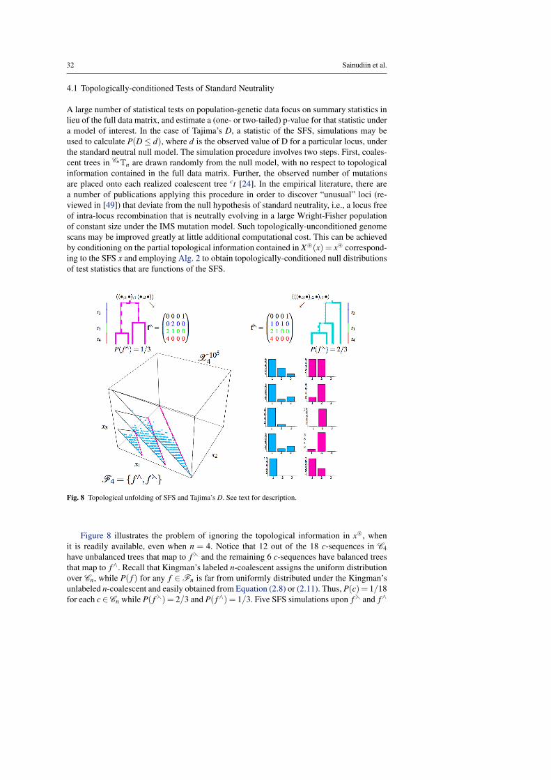
32 Sainudiin et al.

4.1 Topologically-conditioned Tests of Standard Neutrality

A large number of statistical tests on population-genetic data focus on summary statistics inlieu of the full data matrix, and estimate a (one- or two-tailed) p-value for that statistic undera model of interest. In the case of Tajima’s D, a statistic of the SFS, simulations may beused to calculate P(D≤ d), where d is the observed value of D for a particular locus, underthe standard neutral null model. The simulation procedure involves two steps. First, coales-cent trees in CnTn are drawn randomly from the null model, with no respect to topologicalinformation contained in the full data matrix. Further, the observed number of mutationsare placed onto each realized coalescent tree ct [24]. In the empirical literature, there area number of publications applying this procedure in order to discover “unusual” loci (re-viewed in [49]) that deviate from the null hypothesis of standard neutrality, i.e., a locus freeof intra-locus recombination that is neutrally evolving in a large Wright-Fisher populationof constant size under the IMS mutation model. Such topologically-unconditioned genomescans may be improved greatly at little additional computational cost. This can be achievedby conditioning on the partial topological information contained in X~(x) = x~ correspond-ing to the SFS x and employing Alg. 2 to obtain topologically-conditioned null distributionsof test statistics that are functions of the SFS.

Fig. 8 Topological unfolding of SFS and Tajima’s D. See text for description.

Figure 8 illustrates the problem of ignoring the topological information in x~, whenit is readily available, even when n = 4. Notice that 12 out of the 18 c-sequences in C4have unbalanced trees that map to fh and the remaining 6 c-sequences have balanced treesthat map to f∧. Recall that Kingman’s labeled n-coalescent assigns the uniform distributionover Cn, while P( f ) for any f ∈Fn is far from uniformly distributed under the Kingman’sunlabeled n-coalescent and easily obtained from Equation (2.8) or (2.11). Thus, P(c) = 1/18for each c∈Cn while P( fh) = 2/3 and P( f∧) = 1/3. Five SFS simulations upon fh and f∧


are shown as the left and right columns of bar charts, respectively, on the lower right cornerof Fig. 8. The remaining simulated SFS are plotted in the simplexes with a fixed numberof segregating sites s = ∑

n−1i=1 xi contained in X 105

4 , the sample space of SFS with foursampled individuals at 105 sites. Observe how every SFS simulated under f∧ has x3 = 0 andtherefore x~3 = 0, as opposed to those SFS simulated under fh. Crucially, if we do not knowthe hidden f ∈ { fh, f∧} that the observed SFS x was realized upon, then the observationthat x3 > 0 implies that x~3 = 1, and this allows us to unambiguously eliminate f∧ fromthe hidden space of f -sequences we need to integrate over or conditionally simulate from.This set of x~-specific hidden f -sequences is exactly {zn(x~) that we can access withthe proposal Markov chain {F�x~(k)}k∈[n]+ and its importance-reweighed variants. Thus,by means of Alg. 2 that invokes {F�x~(k)}k∈[n]+ and further reweighing by P( f ) we cangenerate the topologically conditioned null distribution of any statistic that is a function ofSFS, including the classical linear combinations of Sect. 3.4 as well as various classical andnon-classical tree shape statistics [40].

The power of classical Tajima’s D test with that of its topologically conditioned versionis compared in Table 1. The significance level α is set at 5% for the standard neutral nullhypothesis H0 and eight alternative hypotheses, namely, H1, . . . ,H8, were explored by in-creasing the recombination rate and/or the growth rate with parameters as shown in Table 1.Here, mφ1 is the scaled per-locus mutation rate, φ2 is the exponential growth rate and ρ isthe scaled per-locus recombination rate. The x~-conditional tests based on Tajima’s D aremore powerful than the unconditional classical tests since a larger proportion of the 104 locisimulated under the alternative models are rejected. All simulations were conducted usingstandard coalescent methods [25].

Table 1 104 loci were simulated under each hypothesised model H0,H1, . . .H8 and tested for the extremenessof the observed Tajima’s D statistic with and without conditioning on the observed x~ in an attempt to rejectthe null hypothesis H0 at significance level α = 5%.

Model: parameters Proportion of loci rejected by null distribution of test statisticsHi : (mφ1,φ2,ρ) PH0 (D≥ d) PH0 (D≥ d|x~) PH0 (D≤ d) PH0 (D≤ d|x~)

H0 : (100,0,0) 0.0495 0.0501 0.0499 0.0501H1 : (100,0,10) 0.0074 0.8640 0.0061 0.0017H2 : (100,0,100) 0.0000 0.9999 0.0000 0.0000H3 : (100,10,0) 0.0000 0.0019 0.0326 0.1759H4 : (100,10,10) 0.0001 0.2023 0.0135 0.0797H5 : (100,10,100) 0.0000 0.5559 0.0006 0.0180H6 : (100,100,0) 0.0000 0.0000 0.1696 0.6882H7 : (100,100,10) 0.0000 0.0002 0.1580 0.6668H8 : (100,100,100) 0.0000 0.0020 0.1321 0.6617

4.2 Exactly Approximate Likelihoods and Posteriors

In computational population genetics, an approximate likelihood or an approximate pos-terior merely refers to the exact likelihood or the exact posterior based on some statisticR(v) = r : V m

n → Rmn . R is called a summary statistic to emphasise the fact that it may

not be sufficient. Approximating the likelihood of the observed statistic ro is often a com-putationally feasible alternative to evaluating the likelihood of the observed data vo. Here,

34 Sainudiin et al.

approximate is meant in the hopeful sense that R may not be a sufficient statistic, i.e., inthe Bayesian sense that P(φ |v) 6= P(φ |r = R(v)), but perhaps approximately sufficient, i.e.,P(φ |v) u P(φ |r) under some reasonable criterion. The exact evaluation of the approximateposterior P(φ |r) involves the exact evaluation of the likelihood P(r|φ) with standard errors.For an arbitrary statistic R, such exact evaluations may not be trivial. However, one may re-sort to the following simulation-based inferential methods termed approximate Bayesian orlikelihood computations in order to approximately evaluate P(φ |r) or P(r|φ), respectively.

4.2.1 ABC

In approximate Bayesian computation or ABC [3], one typically simulates data v ∈ V mn

with a φ -indexed family of measures, such as the Kingman’s n-coalescent superimposed byWatterson’s infinitely-many-sites mutations, after drawing a φ according to its prior distri-bution P(φ), then summarizes it to r = R(v) ∈ Rm

n and finally accepts φ if m(r,ro) ≤ ε ,where the map m : Rm

n ×Rmn → R+ is usually a metric on Rm

n and ε is some non-negativeacceptance-radius. Algorithm 3 details one of the simplest ABC schemes. Approximatelikelihood computation or ALC [52] is similar to ABC, except one typically conducts thesimulations over a finite uniform grid of G points in the parameter space ΦΦ denoted byΦΦ G = {φ (1),φ (2), . . . ,φ (G)}. In a simple ALC, one distributes the computational resourcesevenly over the G parameters in ΦΦ G and approximates the likelihood at φ (i) by the propor-tion of times the summary r of a data v simulated under φ (i) was accepted on the basis ofm(r,ro) ≤ ε . As the grid size and the number of simulations increase, the likelihood esti-mates based on ALC are indistinguishable from the posterior estimate based on ABC undera uniform prior on the appropriate hyper-cuboid containing ΦΦ G.

Algorithm 3 A Simple ABC/ALC Algorithm1: input:

1. a samplable distribution P(v|φ) over V mn indexed by φ ∈ ΦΦ

2. a samplable prior P(φ)3. observed data vo ∈ V (v)m

n and summaries ro = R(vo) ∈Rmn

4. tolerance ε ≥ 05. a map m : Rm

n ×Rmn → R+

6. a large positive integer MAXTRIALS ∈ N

2: output: a sample U ∼ P(φ |rε (ro)) u P(φ |ro) u P(φ |vo) or {},where, rε (ro) := {r : m(r,ro)≤ ε}.

3: initialize: TRIALS← 0, SUCCESS← false, U ←{}4: repeat5: φ ← P(φ) {DRAW from Prior}6: v← P(v|φ) {SIMULATE data}7: r← R(v) {SUMMARIZE data}8: if m(r,ro)≤ ε then {COMPARE summaries and ACCEPT/REJECT parameter}9: U ← φ , SUCCESS← true

10: end if11: TRIALS← TRIALS+112: until TRIALS≥ MAXTRIALS or SUCCESS← true13: return: U

Statistical justification of ALC and ABC methods rely on the summary statistic R beingclose to the typically unknown sufficient statistic and thereby producing reasonably approx-imate likelihood and posterior. However, as R gets closer to the sufficient statistic one has tomake the acceptance-radius ε unreasonably large to increase the acceptance rate of the pro-posed φ . For instance, current ALC and ABC methods have unacceptably low acceptance


rates for a reasonably small ε if r is taken as the SFS. But when ε is too large we gain littleinformation from the simulations.

Let us examine the ‘ε-dilemma’ under the ABC framework in detail. Analogous argu-ments also apply for the ALC framework. In ABC, samples are drawn from an ε-specificapproximation of P(φ |ro). Since, rε(ro) := {r : m(r,ro)≤ ε}, we are making the followingposterior approximation of the ultimately desired P(φ |vo) :

P(φ |vo) u

{P(φ |ro) = P(φ |{v : R(v) = R(vo) = ro}) if: ε = 0P(φ |rε(ro)) = P(φ |{v : m(R(v),R(vo))≤ ε}) if: ε > 0.

The assumed approximate sufficiency of the statistic R, i.e., P(φ |vo) u P(φ |ro), terms theposterior P(φ |ro) approximate. Furthermore, the non-zero acceptance-radius ε , for reasonsof computational efficiency, yields the further ε-specific approximate posterior P(φ |rε(ro)).In the extremal case, the approximate posterior P(φ |r∞(ro)) equals the prior P(φ), and wehave gained no information from the experiment. Furthermore, there is no guarantee that acomputationally desirable metric m is also statistically desirable, i.e., produce reasonablyapproximate posterior samples.

Considerable effort is expended in fighting this ‘ε-dilemma’ by say (1) smoothing them(r,ro)’s [3] or (2) making use of local Monte Carlo samplers [35] or (3) finding the rightsequence of ε’s under the appropriate metric m [44] in order to obtain the optimal trade-offbetween efficiency and accuracy (see [4] for a recent review of ABC methods). It is difficultto ensure that such sophisticated battles against the ‘ε-dilemma’ that arise in the simulation-based inferential approaches of ABC and ALC do not confound the true posterior P(φ |ro)or the true likelihood P(ro|φ). Thus, both ABC and ALC methods may benefit from exactmethods that can directly produce the likelihood P(ro|φ), for at least a class of summarystatistics. They may also benefit from a systematic treatment of the relative information indifferent sets of summary statistics obtainable with exact methods.

4.2.2 ABCDE

For a large class of statistics, namely the SFS and its various linear combinations, our ap-proach allows the acceptance radius ε to equal zero. This is achieved by Monte Carlo sim-ulations of the controlled lumped coalescent Markov chain {F�x~(k)}k∈[n]+ of Alg. 2 andfurther reweighing by P( f ) to evaluate P(x|φ) in Eq. (3.10) and P(r|φ) in Eq. (3.14). There-fore our approach yields an exact evaluation of the desired approximate posterior P(φ |r)and amounts to ABCDE or ABC done exactly.

4.2.3 Parameter Estimation in an Exponentially Growing Population

We estimate the locus-specific scaled mutation rate mφ ∗1 and the exponential growth rate φ ∗2based on the observed SFS at one non-recombining locus of length m from n samples. Theperformance of our estimator is assessed over 1,000 data sets that were simulated underthe standard neutral model with mφ ∗1 = 10.0 and φ ∗2 = 0.0 (for human data mφ ∗1 = 10.0implies a locus of length 10kbp, i.e., m = 104) [25]. Our choices of φ ∗1 and m are biologicallymotivated by a previous study on human SNP density [42]. Our point estimate (mφ1, φ2)of (mφ ∗1 ,φ ∗2 ) based on the SFS x is the maximum aposteriori estimate obtained from ahistogram estimate of the posterior P(φ |x). The histogram is based on a uniform grid of101×101 parameter points φ = (φ1,φ2) over our rectangular uniform prior density ((100−1/10000)100)−111{[0.0001,100],[0,100]}(φ1,φ2).

36 Sainudiin et al.

Table 2 Performance of our estimator of mφ∗1 and φ∗2 based on SFS (see text).

n performance of mφ1 performance of φ2 performance of (mφ1, φ2)√se bs C99%

√se bs C99% C99% quartiles of ˘K

4 40 28 .545 41 26 .185 .828 {0.062,0.085,0.143}5 35 22 .584 34 20 .236 .832 {0.073,0.102,0.167}6 30 19 .602 32 18 .343 .824 {0.081,0.109,0.178}7 27 16 .660 29 14 .410 .838 {0.089,0.126,0.209}8 23 13 .687 25 11 .474 .852 {0.096,0.142,0.235}9 20 11 .712 23 10 .554 .872 {0.102,0.155,0.263}10 19 10 .711 25 11 .604 .858 {0.106,0.164,0.294}

Our performance measures can help make natural connections to the theory of approx-imate sufficiency [6], as we not only measure the bias (bs), root-mean-squared-error (

√se)

and the marginal and joint 99% empirical coverage (C99%) but also the data-specific vari-ation in the concentration of the posterior distribution as summarized by the quartiles of

˘K , the Kullback-Leibler divergence between the posterior histogram estimate and the uni-form prior that is rescaled by the prior’s entropy. Table 2 gives the maximum aposteri-ori estimate of (mφ ∗1 ,φ ∗2 ) by a Monte Carlo sum over φ2-specific epoch-time vectors inTn := (0,∞)n−1 and every x~-specific hidden f -sequence in {zn(x~) by means of Alg. 2that invokes {F�x~(k)}k∈[n]+ .

We also obtained maximum aposteriori point estimate (mφ1, φ2) of (mφ ∗1 ,φ ∗2 ) = (10,0)based on (s,z) and (s,z,x~) of the SFS x. Our ABCDE estimators are equivalent to exactlyapproximate Bayesian computations (with ε = 0) as we integrate exhaustively over all SFSin R−1((s,z)′) when we compute P(φ |(s,z)) or P(φ |(s,z,x~)). For the same set of simulateddata of Table 2 the joint empirical coverage significantly suffered at about 50% for theestimator that only used (s,z). By using additional topological information, the estimatorbased on (s,z,x~) had a better coverage that improved with sample size (between 61% and76%). We also restrict the sample size to exhaustively integrate over the fiber R−1(s,z′)and avoid expositions on Monte Carlo samplers over R−1(s,z′) for brevity. Contrastingly,the coverage was nearly perfect when the entire BIM was used to estimate the parametersthrough an importance sampler [46].

When ABC is done exactly, it is clear that using a few coarse linear summaries of theSFS, even after a topological conditioning by x~, is not only computationally inefficientbut also provides significantly less information when compared to using the entire SFS.Nonetheless, these computations over population genetic fibers shed algebraic insights andprovide exact benchmarks against which one can compare, correct and improve simulation-intensive ABC/ALC algorithms in the current molecular population genetic literature thatignore topological information up to sufficient equivalence classes in the hidden space ofgenealogies.

Authors’ Contributions KT and RS posed the ABCDE problem. RS developed the con-trolled lumped chain {F�x~(k)}k∈[n]+ based on discussions with PD, RG and GM. RS codedall related modules of LCE-0.1 with support from KT. JH efficiently re-implemented Alg. 2.RS developed the samplers over population genetic fibers based on discussions with JB,MS and RY. RY and MS conducted the algebraic statistical computations in LattE andMacaulay 2, respectively. RS wrote the first draft and incorporated comments made by thecoauthors.


Acknowledgements RS was supported by an NSF/NIGMS grant DMS-02-01037 and a research fellowshipfrom the Royal Commission for the Exhibition of 1851 under the sponsorship of PD during the course ofthis study. JH was supported by an Allan Wilson Summer Studentship. RY was supported by NIGMS grant1R01GM086888. Comments from two anonymous referees greatly improved the manuscript. RS thanks Ce-line Becquet for discussions on summary statistics of structured populations, Mike Steel for [29, Definition6.3.1], Jesse Taylor for [32, 5.2], Joe Watkins for the articulation of Definition 2, Michael Nussbaum andSimon Tavare for discussions on approximate sufficiency and Scott Williamson for generous introductions tothe site frequency spectrum.

References

1. Bahlo M, Griffiths R (1996) Inference from gene trees in a subdivided population. The-oret Pop Biol 57:79–95

2. Barvinok A (1994) Polynomial time algorithm for counting integral points in polyhedrawhen the dimension is fixed. Math of Operations Research 19:769–779

3. Beaumont M, Zhang W, Balding D (2002) Approximate Bayesian computation in pop-ulation genetics. Genetics 162:2025–2035

4. Bertorelle G, Benazzo A, Mona S (2010) ABC as a exible framework to estimate de-mography over space and time: some cons, many pros. Molecular Ecology 19:2609–2625

5. Birkner M, Blath J (2008) Computing likelihoods for coalescents with multiple colli-sions in the innitely many sites model. J Math Biol 57:435–465

6. Cam LL (1964) Sufficiency and approximate sufficiency. Ann Math Stats 35:1419–1455

7. Casanellas M, Garcia L, Sullivant S (2005) Catalog of small trees. In: Pachter L, Sturm-fels B (eds) Algebraic statistics for computational biology, Cambridge University Press,pp 291–304

8. Diaconis P, Sturmfels B (1998) Algebraic algorithms for sampling from conditionaldistributions. Annals of Statistics 26:363–397

9. Duflo M (1997) Random Iterative Models. Springer10. Erdos P, Guy R, Moon J (1975) On refining partitions. J London Math Soc (2) 9:565–

57011. Ewens W (1972) The sampling theory of selectively neutral alleles. Theoret Pop Biol

3:87–11212. Ewens W (1974) A note on the sampling theory of infinite alleles and infinite sites

models. Theoret Pop Biol 6:143–14813. Ewens W (2000) Mathematical Population Genetics, 2nd edn. Springer14. Fay J, Wu C (2000) Hitchhiking under positive darwinian selection. Genetics 155:1405–

141315. Felsenstein J (1981) Evolutionary trees from DNA sequences: a maximum likelihood

approach. Journal of Molecular Evolution 17:368–37616. Felsenstein J (2006) Accuracy of coalescent likelihood estimates: Do we need more

sites, more sequences, or more loci? Molecular Biology and Evolution 23:691–70017. Grayson D, Stillman M (2004) Macaulay 2, a software system for research in algebraic

geometry. Available at www.math.uiuc.edu/Macaulay218. Griffiths R, Tavare S (1994) Ancestral inference in population genetics. Stat Sci 9:307–

31919. Griffiths R, Tavare S (1996) Markov chain inference methods in population genetics.

Math Comput Modelling 23:141–158

www.math.uiuc.edu/Macaulay2

38 Sainudiin et al.

20. Griffiths R, Tavare S (2003) The genealogy of a neutral mutation. In: Green P, Hjort N,Richardson S (eds) Highly Structured Stochastic Systems, Oxford University Press, pp393–412

21. Hastings W (1970) Monte Carlo sampling methods using Markov chains and their ap-plications. Biometrika 57:97–109

22. Hemmecke R, Hemmecke R, Malkin P (2005) 4ti2 version 1.2—computation of Hilbertbases, Graver bases, toric Grobner bases, and more. Available at www.4ti2.de

23. Hosten S, Khetan A, Sturmfels B (2005) Solving the likelihood equations. Found Com-put Math 5(4):389–407

24. Hudson R (1993) The how and why of generating gene genealogies. In: Clark A, Taka-hata N (eds) Mechnisms of Molecular Evolution, Sinauer, pp 23–36

25. Hudson R (2002) Generating samples under a Wright-Fisher neutral model of geneticvariation. Bioinformatics 18:337–338

26. Iorio M, Griffiths R (2004) Importance sampling on coalescent histories. I.Adv Appl Prob 36:417–433

27. Jones G, Hobert J (2001) Honest exploration of intractable probability distributions viaMarkov chain Monte Carlo. Statistical Science 16(4):312–334

28. Jukes T, Cantor C (1969) Evolution of protein molecules. In: Munro H (ed) MammalianProtein Metabolism, New York Academic Press, pp 21–32

29. Kemeny, Snell (1960) Finite Markov Chains. D. Van Nostrand Co.30. Kendall D (1975) Some problems in mathematical genealogy. In: Gani J (ed) Perspec-

tives in Probability and Statistics, Academic Press, pp 325–34531. Kingman J (1982) The coalescent. Stochastic Processes and their Applications 13:235–

24832. Kingman J (1982) On the genealogy of large populations. Journal of Applied Probabil-

ity 19:27–4333. Kolmogorov A (1942) Sur l’estimation statistique des parameteres de la loi de gauss.

Bull Acad Sci URSS Ser Math 6:3–3234. Loera JD, Haws D, Hemmecke R, Huggins P, Tauzer J, Yoshida R (2004) Lattice

Point Enumeration: LattE, software to count the number of lattice points inside arational convex polytope via barvinok’s cone decomposition. Available at www.math.ucdavis.edu/~latte

35. Marjoram P, Molitor J, Plagnol V, Tavare S (2003) Markov chain Monte Carlo withoutlikelihoods. Proc Natl Acad Sci USA 100:15,324–15,328

36. Metropolis N, Rosenbluth A, Rosenbluth M, Teller A, Teller E (1953) Equations of statecalculations by fast computing machines. Jnl Chem Phys 21:1087–1092

37. Mossel E, Vigoda E (2005) Phylogenetic MCMC algorithms are misleading on mixturesof trees. Science 309:2207–2209

38. Mossel E, Vigoda E (2006) Limitations of Markov chain Monte Carlo algorithms forBayesian inference of phylogeny. Ann Appl Probab 16(4):2215–2234

39. Rosenblatt M (1974) Random Processes. Springer-Verlag40. Sainudiin R, Stadler T (2009) A unified multi-resolution coalescent: Markov lumpings

of the Kingman-Tajima n-coalescent – UCDMS Research Report 2009/4, april 5, 2009(submitted). Available at http://www.math.canterbury.ac.nz/~r.sainudiin/preprints/SixCoal.pdf

41. Sainudiin R, York T (2009) Auto-validating von Neumann rejection sampling fromsmall phylogenetic tree spaces. Algorithms for Molecular Biology 4:1

42. Sainudiin R, Clark A, Durrett R (2007) Simple models of genomic variation in humanSNP density. BMC Genomics 8:146

www.math.ucdavis.edu/~latte

www.math.ucdavis.edu/~latte

http://www.math.canterbury.ac.nz/~r.sainudiin/preprints/SixCoal.pdf

http://www.math.canterbury.ac.nz/~r.sainudiin/preprints/SixCoal.pdf


43. Semple C, Steel M (2003) Phylogenetics. Oxford University Press44. Sisson S, Fan Y, Tanaka M (2007) Sequential Monte Carlo without likelihoods.

Proc Natl Acad Sci USA 104:1760–176545. Slatkin M (2002) A vectorized method of importance sampling with applications to

models of mutation and migration. Theoret Pop Biol 62:339–34846. Stephens M, Donnelly P (2000) Inference in molecular population genetics.

J R Statist Soc B 62:605–65547. Tajima F (1989) Statistical method for testing the neutral mutation hypothesis by dna

polymorphism. Genetics 123:585–59548. Tavare S (1984) Line-of-descent and genealogical processes, and their applications in

population genetics models. Theoretical Population Biology 26:119–16449. Thornton K, Jensen JD, Becquet C, Andolfatto P (2007) Progress and prospects in map-

ping recent selection in the genome. Heredity 98:340–34850. Wakeley J (2007) Coalescent Theory: An Introduction. Roberts & Co.51. Watterson G (1975) On the number of segregating sites in genetical models without

recombination. Theor Popul Biol 7:256–27652. Weiss G, von Haeseler A (1998) Inference of population history using a likelihood

approach. Genetics 149:1539–154653. Yang Z (2000) Complexity of the simplest phylogenetic estimation problem. Proceed-

ings Royal Soc London B Biol Sci 267:109–119

Experiments with the Site Frequency Spectrum

Documents

Transcript of Experiments with the Site Frequency Spectrum