EXPERIMENTAL INVESTIGATION OF A MAGNETIC INDUCTION PEBBLE-BED

HEATER WITH APPLICATION TO NUCLEAR THERMAL PROPULSION

by

ROBERT MICHAEL TALLEY

JOHN BAKER, COMMITTEE CHAIR

CLARK MIDKIFF

ROBERT TAYLOR

A THESIS

Submitted in partial fulfillment of the requirements

for the degree of Master of Science in the

Department of Mechanical Engineering

in the Graduate School of

The University of Alabama

TUSCALOOSA, ALABAMA

2014

Copyright Robert Michael Talley 2014

ALL RIGHTS RESERVED

ii

ABSTRACT

NASA explored the idea of nuclear thermal rockets in the 1950’s and 60’s and has

recently shown interest in reviving the nuclear rocket program in an attempt to reach manned

mission to Mars by 2035. One problem with nuclear rockets is finding ways to test them inside

the atmosphere. NASA’s Stennis Space Center has considered using a non-nuclear device to

simulate a nuclear reactor during testing. The reactor is responsible for heating the propellant to

over 1,922 K (3,000 °F), so the reactor simulator should be capable of heating to this

temperature. A pebble-bed heater at Glenn Research Center was used for nuclear rocket testing

in the past; however, the device no longer exists. This particular pebble-bed heater used hot

gases to heat the pebble bed made of high melting temperature ceramics and was able to reach

2,755 K (4,500 °F) but could only sustain the temperature for 30 seconds at most.

If the pebbles were heated by magnetic induction, then heat would consistently be

generated within the heater, and tests could run longer. Magnetic induction heats a ferrous metal

by inducing a current on its surface and by rapidly reversing a magnetic field surrounding the

metal. Unfortunately, it was found that a magnetic induction pebble-bed heater using steel could

not reach 1,922 K (3,000 °F) due to the Curie and melting temperatures. However, the device

could be used if a higher melting temperature metal was found that was also magnetic.

A small-scale pebble-bed heater heated by magnetic induction was designed, built, and

tested to analyze its behavior at 27 different combinations of flow rates, pebble sizes, and power

levels. The temperature changes were recorded for each test. With this data, a relationship

between dimensionless heat transfer, dimensionless power, and Reynolds number was found.

iii

LIST OF ABBREVIATIONS AND SYMBOLS

Aair

Asteel

B

cp

DMM

DPT

go

GRC

H

I

Isp

kair

kplastic

ksteel

Lc_air

Lc_steel

mballs

MOSFET

NHT

Effective area of air in pipe cross section

Effective area of steel in pipe cross section

Flux density

Specific heat at constant pressure

Digital Multimeter

Differential Pressure Transducer

Acceleration due to gravity

Glenn Research Center

Magnetizing Force

Current

Specific Impulse

Thermal conductivity of air

Thermal conductivity of plastic

Thermal conductivity of steel

Characteristic length of air in the pipe

Characteristic length of carbon steel in the pipe

Mass flow rate

Mass of all balls inside the cylinder

Metal-Oxide Semiconductor Field-Effect Transistor

Dimensionless Heat Transfer

ii

iv

NP

NASA

NERVA

NPT

NRS

NTP

NTR

Qcond

Qconv

Qloss_wall

Qremaining

P

PBH

Rair

Rsteel

Re

rin

rout

SAballs

SSC

T

Dimensionless Power

National Aeronautics and Space Administration

Nuclear Engine for Rocket Vehicle Application

National Pipe Thread

Nuclear Reactor Simulator

Nuclear Thermal Propulsion

Nuclear Thermal Rocket

Power given to heat the pebbles by conduction

Power given to heat the air by convection

Power lost due to heat leaving through the pipe wall

Power not used for convection or escaping through the pipe wall

Power

Pebble-Bed Heater

Resistance of air

Resistance of carbon steel

Reynolds number

Inner pipe radius

Outer pipe radius

Surface area of all balls inside the chamber

Stennis Space Center

Force of thrust

iii

v

U

V

Vpipe

Vsteel

ΔP

ΔT

δ

ω

μ

σ

ρ

ν

Velocity of air

Voltage

Volumetric Flow Rate

Volume of the inside of the pipe

Volume of steel inside the pipe

Change in pressure through the heating chamber

Change in temperature through the heating chamber

Skin depth

Frequency of current

Permeability of material

Electrical conductivity of material

Density

Kinematic viscosity

iv

vi

ACKNOWLEDGMENTS

I have several people to thank for assisting me in fulfilling my research and thesis. Most

importantly, I would like to thank Dr. John Baker for his excellent guidance and wisdom over the

last two years. Dr. Baker has been very helpful and always made time for me when I needed him.

I would also like to thank Dr. Clark Midkiff and Dr. Robert Taylor for agreeing to be my

committee members, for their input on my thesis paper, and for their assistance throughout my

graduate program. Graduate school would not have been possible without the Graduate Teaching

Assistantship granted to me by Dr. Keith Williams, Dr. Hwan Sic Yoon, and the Mechanical

Engineering department.

I am extremely indebted to Mr. David Coote and Dr. Harry Ryan at NASA’s Stennis

Space Center for hiring me as an intern in the summer of 2012, training and educating me over

my term, and providing me with valuable experience that assisted in the making of this thesis.

Ken Dunn and the men at The University of Alabama’s machine shop were very

generous about cutting and sweating some pipe pieces for me on short notice and machining

other parts of the experiment. The University of Alabama’s 3D Printing Lab also did a

phenomenal job printing off one of the key components of the experiment. Every purchase I

made had to go through Ms. Lisa Hinton, so I would like to thank her for her hard work as well.

Ms. Betsy Singleton and Ms. Lynn Hamric were also a huge help throughout my graduate

studies. Lastly, I would like to thank Mindy, my family, and my friends for supporting my

decision to attend graduate school at The University of Alabama and being there for me along

the way.

v

vii

CONTENTS

ABSTRACT………………………………………………………………………………………ii

LIST OF ABBREVIATIONS AND SYMBOLS………………………………………………...iii

ACKNOWLEDGMENTS………………………………………………….………………..…....vi

LIST OF TABLES……………………………………………….…………….……...…….…..viii

LIST OF FIGURES……………………………………………………………………..………...ix

1. INTRODUCTION………………………………………….………..………………………...1

2. BACKGROUND AND LITERATURE REVIEW………………….………………………...3

a. Nuclear Thermal Propulsion…………………………………………………………………..3

b. Pebble-Bed Heater..…………………….……………………………………………..………7

c. Magnetic Induction Heating…………………………………………………………...……..10

3. EXPERIMENT APPROACH………………………………………………………….…….18

a. Designing the Pebble-Bed Heater..……………………….……………………………….....18

b. Constructing the Pebble-Bed Heater..……………………………….…………………...…..30

c. Designing the Induction Heater…………………………….…………….………………….37

d. Constructing the Induction Heater………………………………………….………………..44

4. TESTING PROCEDURE………………………………………………………………...….48

5. RESULTS…………………………………………………………………………………....53

6. DISCUSSION…………………………………………………………………..……………65

REFERENCES……………………………………………………………………………….…..73

APPENDIX……………………………………………………………………………...……….79

vi

viii

LIST OF TABLES

1. Temperature data from all 27 tests in °F, °C, and K………………………….……….……..53

2. Volume, surface area, and mass for the different ball sizes in imperial and metric units..…..55

3. Efficiency and Heat Transfer data…………….……………………………………………...61

4. Additional Heat Transfer data………………………………………………………………..61

5. Reynolds number and Dimensionless Power data………………………………….………..62

6. Inefficiency data from all 27 experiments…………………………………………………...64

vii

ix

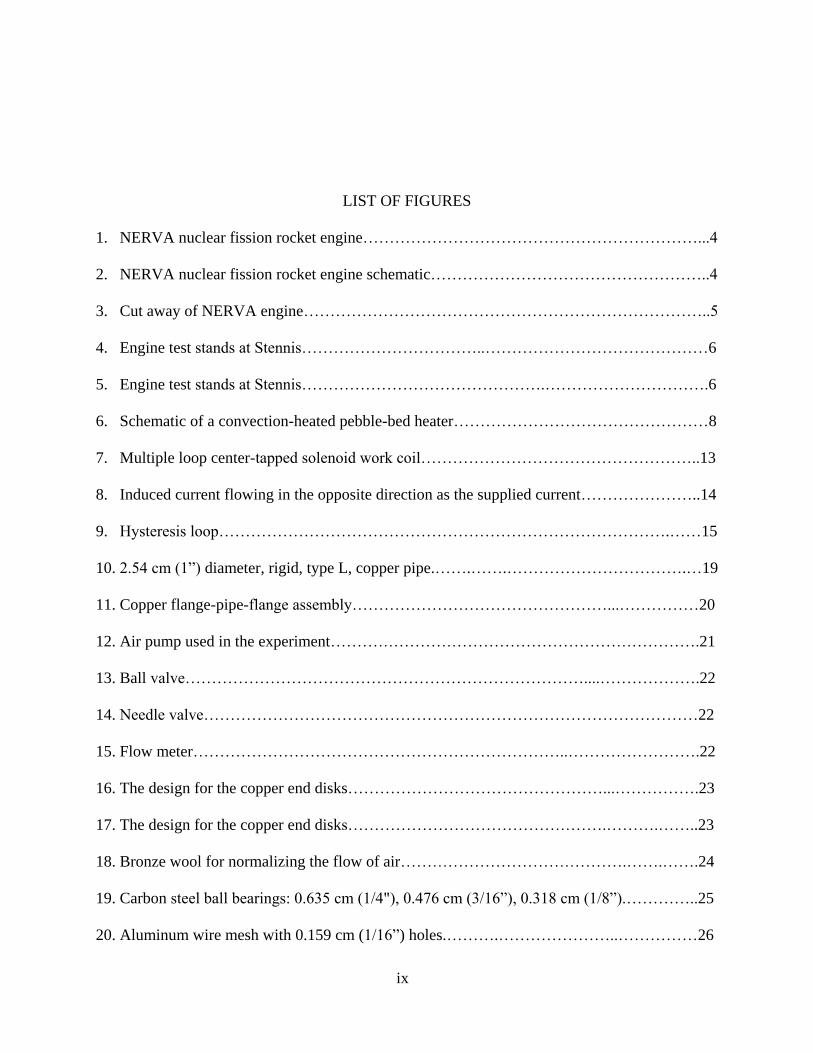
LIST OF FIGURES

1. NERVA nuclear fission rocket engine………………………………………………………...4

2. NERVA nuclear fission rocket engine schematic……………………………………………..4

3. Cut away of NERVA engine…………………………………………………………………..5

4. Engine test stands at Stennis……………………………..……………………………………6

5. Engine test stands at Stennis……………………………………….………………………….6

6. Schematic of a convection-heated pebble-bed heater…………………………………………8

7. Multiple loop center-tapped solenoid work coil……………………………………………..13

8. Induced current flowing in the opposite direction as the supplied current…………………..14

9. Hysteresis loop………………………………………………………………………….……15

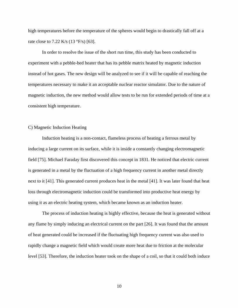
10. 2.54 cm (1”) diameter, rigid, type L, copper pipe.…….…….…………………………….…19

11. Copper flange-pipe-flange assembly…………………………………………...……………20

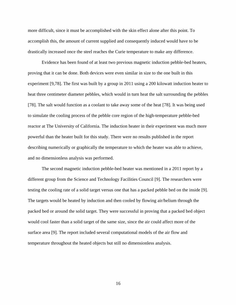
12. Air pump used in the experiment…………………………………………………………….21

13. Ball valve…………………………………………………………………....……………….22

14. Needle valve…………………………………………………………………………………22

15. Flow meter……………………………………………………………..…………………….22

16. The design for the copper end disks…………………………………………...…………….23

17. The design for the copper end disks………………………………………….……….……..23

18. Bronze wool for normalizing the flow of air…………………………………….…….…….24

19. Carbon steel ball bearings: 0.635 cm (1/4"), 0.476 cm (3/16”), 0.318 cm (1/8”).…………..25

20. Aluminum wire mesh with 0.159 cm (1/16”) holes.……….…………………..……………26

viii

x

21. T-type thermocouple with a 15.24 cm (6”) probe………….….……..………………..……..27

22. Thermocouple reader…………………………………………………………..…………….28

23. Differential pressure transducer with DMM clips attached to output…….….…....…….…..29

24. Solidworks drawing of pipe and flange assembly…………………………...………………30

25. Schematic of the pebble-bed heater experiment……………………………………………..30

26. Experiment configuration from air pump to flow meter………………………….………….32

27. Construction up to the first pipe section……………………………….…………………….32

28. Thermocouple probe attached to the copper spacer…………………………………………33

29. DPT tube attached to the copper spacer……………………………………………………..33

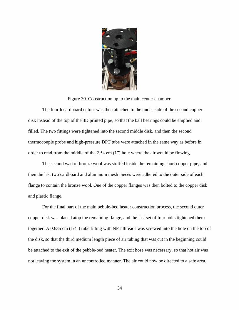
30. Construction up to the main center chamber………………………...………………………34

31. Completed stand and pebble-bed heater…………………………………….……………….36

32. Rear of thermocouple reader with thermocouples connected to ports 1 and 2……….…...…36

33. The internal wiring of the DPT………………………………………………………..……..37

34. The wiring diagram of the DPT…………………………………………..………………….37

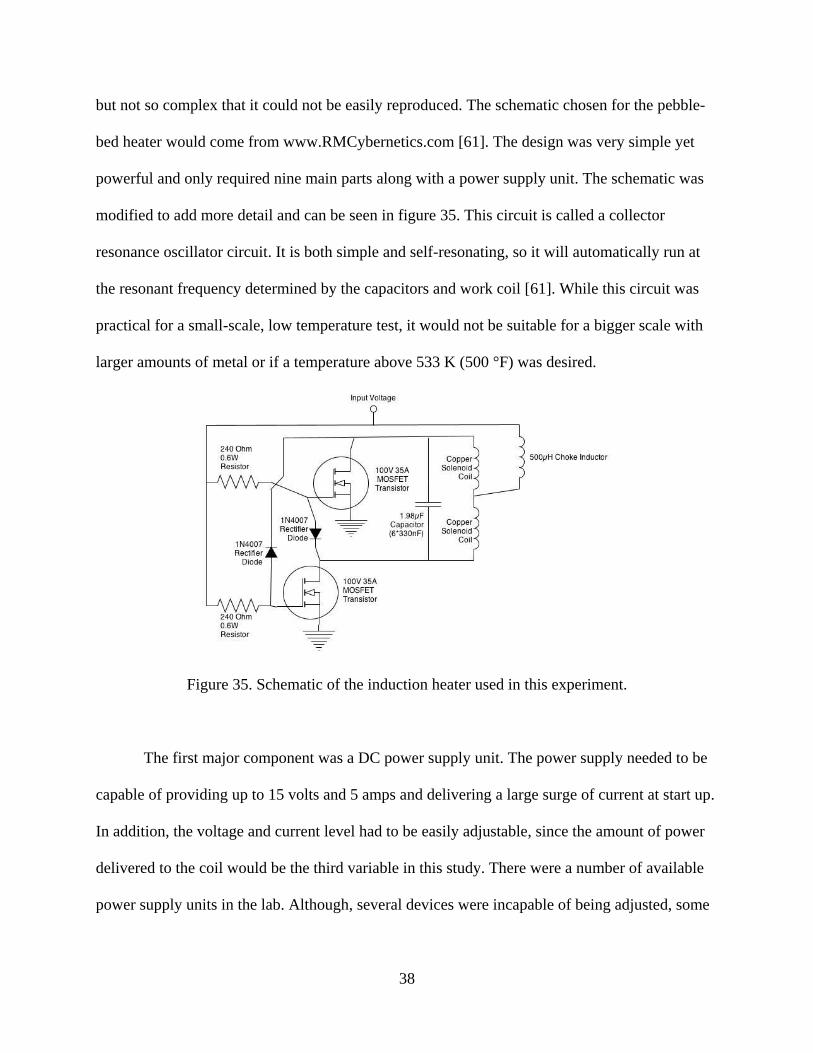
35. Schematic of the induction heater used in this experiment………………………….………38

36. DC power supply with electronic display and adjustable voltage…………………..…….…39

37. 500 µH choke inductor…………………………………………………………………….…41

38. Six 330 nF capacitors combined in parallel with each other and the work coil……….….…41

39. MOSFET and heat sink……………………………………………………………….…...…43

40. Solenoid made from copper pipe..……………..…………………………………….………44

41. The final coil for the induction heater……………………………………………….………45

ix xi

42. Induction heater circuit and wiring…………….…………………………………………….47

43. Induction heater circuit and wiring……………………………………………….………….47

44. Voltage-current relationship for 0.635 cm (1/4”) balls………………………………………49

45. Voltage-current relationship for 0.476 cm (3/16”) balls……………………………………..51

46. Voltage-current relationship for 0.0.318 cm (1/8”) balls…………………………………….52

47. Temperature change vs power supplied at fixed flow rate for 0.635 cm (1/4") balls………..54

48. Temperature change vs power supplied at fixed flow rate for 0.476 cm (3/16") balls………54

49. Temperature change vs power supplied at fixed flow rate for 0.318 cm (1/8") balls………..55

50. Power applied through the solenoid vs heating efficiency with 0.476 cm (3/16”) balls…….57

51. Resistance diagram for air and steel…………………………………………………………58

52. Sine wave and frequency of the experiment…………………………………………………59

53. Dimensionless relationship in a magnetic induction pebble-bed heater….…….…….…..….60

1

CHAPTER 1

INTRODUCTION

From 1955 to 1972 NASA explored the idea of nuclear thermal propulsion and nuclear

thermal rockets with the NERVA (Nuclear Engine for Rocket Vehicle Application) program.

NERVA was successful in building and testing a nuclear rocket engine, but the engine was never

approved and used on a rocket in outer space. In 1972 the program was cancelled due to lack of

funding.

Recently, NASA has been interested in reviving the idea of nuclear thermal rockets

(NTR). Nuclear rockets provide double the specific impulse (Isp) compared to that of current

chemical rockets and would therefore make manned exploration to Mars possible by

significantly reducing the round trip time [2]. One major obstacle of the nuclear thermal rocket

revival effort that did not exist in the 1950’s and 60’s is testing the nuclear engines in the earth’s

atmosphere. Several solutions for testing the engines were proposed at NASA’s Stennis Space

Center (SSC). One of the solutions being to find a nuclear reactor simulator (NRS) that was non-

nuclear but could still heat the hydrogen rocket propellant to the same temperature that the

nuclear reactor would, which was between 1,922 K and 3,033 K (3,000 °F and 5,000 °F). The

most promising simulator was a pebble-bed heater (PBH) [48,58,59]. NASA currently has at

least two pebble-bed heaters—one at Glenn Research Center and one at Stennis Space Center

[25,34,43].

In order to simulate a nuclear reactor, the pebble-bed heater would first need to heat a

large number of small steel or ceramic spheres in an internal chamber and raise their temperature

to over 1,922 K (3,000 °F) before running the hydrogen propellant through the pebble bed. The

hydrogen would heat up as it passed over the spheres and then make its way to the rocket engine

2

interface. This would allow the engineers to test their rocket engine under nuclear conditions and

hopefully produce a working product without ever using nuclear materials.

Current pebble-bed heaters at NASA facilities use convection and hot gases to heat the

spheres inside the pebble-bed heating chamber and have been known to reach temperatures up to

2,755 K (4,500 °F). However, this convection method only allows for a limited testing window

as the spheres will quickly cool off as the heat is taken away from them, and the hydrogen will

no longer exit at the desired temperature. This will result in a very short test time for an engine

that would normally be used for at least several minutes.

The purpose of this research was twofold. The first reason being to determine if magnetic

induction could be used instead of hot gases when heating the spheres inside the pebble-bed

heater. This would achieve longer run times at a consistent high temperature during nuclear

engine testing. Secondly, a dimensionless analysis would be performed in order to predict the

outcome of future pebble-bed heaters. Therefore, the research also included an experiment that

demonstrates the capabilities of a small-scale magnetic induction pebble-bed heater and the

effects of certain variables on the system. A small-scale pebble-bed heater and an induction

heater were designed, constructed, and tested in order to analyze the system’s behavior. The

experiment was built so that the variables could be easily monitored and varied. The pebble-bed

heater was tested at a series of flow rates, power levels, and pebble sizes.

3

CHAPTER 2

BACKGROUND AND LITERATURE REVIEW

A) Nuclear Thermal Propulsion

NASA has a stated goal of sending humans beyond the moon by 2025 and sending

humans on a roundtrip mission to Mars by 2035 [5]. With its increased thrust-to-weight ratio and

higher specific impulse, the best option for manned missions beyond the moon is nuclear thermal

propulsion [2].

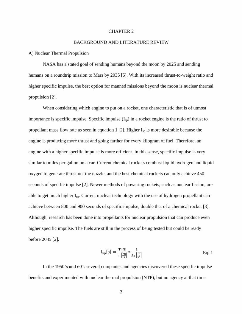
When considering which engine to put on a rocket, one characteristic that is of utmost

importance is specific impulse. Specific impulse (Isp) in a rocket engine is the ratio of thrust to

propellant mass flow rate as seen in equation 1 [2]. Higher Isp is more desirable because the

engine is producing more thrust and going farther for every kilogram of fuel. Therefore, an

engine with a higher specific impulse is more efficient. In this sense, specific impulse is very

similar to miles per gallon on a car. Current chemical rockets combust liquid hydrogen and liquid

oxygen to generate thrust out the nozzle, and the best chemical rockets can only achieve 450

seconds of specific impulse [2]. Newer methods of powering rockets, such as nuclear fission, are

able to get much higher Isp. Current nuclear technology with the use of hydrogen propellant can

achieve between 800 and 900 seconds of specific impulse, double that of a chemical rocket [3].

Although, research has been done into propellants for nuclear propulsion that can produce even

higher specific impulse. The fuels are still in the process of being tested but could be ready

before 2035 [2].

[ ] [ ]

[

]

[

]

In the 1950’s and 60’s several companies and agencies discovered these specific impulse

benefits and experimented with nuclear thermal propulsion (NTP), but no agency at that time

Eq. 1

4

succeeded in producing a space-ready, approved engine and eventually lost funding. One of the

most successful nuclear programs was NERVA (Nuclear Engine for Rocket Vehicle

Application), which was headed by NASA and the US Atomic Energy Commission [45]. The

NERVA team was able to build and test a nuclear rocket engine as seen in figures 1 and 2.

Figures 1 and 2. NERVA nuclear fission rocket engine and schematic.

Credit: NASA (Public Domain) [7,36].

NER A’s engine was a nuclear fission, solid-core, flight-rated, graphite engine designed

to provide 333 kN (74,861 lb) of thrust with an Isp of 825 seconds, and weighing 92.5 kN (20,800

lb) [55]. The NERVA engine had a ten-hour supply of fuel and could power up and down as

many as 60 times allowing it to conserve fuel when thrust was not needed [55]. It consisted of

three main sections: the turbopumps, the nuclear reactor, and the nozzle (Figure 3); however, this

discussion will focus mainly on the reactor [36]. The hydrogen would start in the storage tank,

make its way down to cool the nozzle, proceed to the turbopumps, run through the nuclear

fission reactor, and blast out of the nozzle, generating thrust [55]. Despite its apparent success,

there were problems with the overall design and especially the reactor [21]. Several of the main

5

issues with the reactor were caused by high operating temperatures in a corrosive atmosphere as

well as drastic temperature variations across the reactor [21]. This caused several reactors to fail

in the testing process. These problems, in addition to others, led to the downfall of the project,

and in 1972 the NERVA engine was decommissioned.

Figure 3. Cut away of NERVA engine. Credit: NASA (Public Domain). [36].

There was another promising program at the same time as NERVA called Project Rover

which existed from 1955 to 1973. The Rover team was able to run 22 full power tests for a total

duration of 109 minutes [30]. The engine operated at a thrust of 929,678 N (209,000 lb) and a

specific impulse just over 900 seconds with the hydrogen propellant heated to 2,533 K (4,100 °F)

[30]. As successful as Rover was, it was forced to shut down due to the insufficient technology

of the time and lack of funding, as was the case with NERVA. Since its closing, the facilities

have been torn down, so very little of Project Rover remains. After NER A and Rover’s

decommission, several companies and programs have tried to bring back the nuclear rocket

engine program using similar technology, but none have succeeded.

Once more, NASA is attempting to develop a nuclear rocket engine in order to meet the

benchmark of sending a man on a roundtrip mission to Mars by 2035. NASA has asked their

Stennis Space Center engine testing facility (Figures 4 and 5) to run and analyze the nuclear

6

rocket engine on their test stands after the engine has been constructed [48,58,59]. The engineers

at NASA are studying the pros and cons of the NERVA and Rover programs, so that they can

recreate and improve the nuclear engine. However, the testing process will prove to be a major

setback because the world is much more environmentally and safety conscious than it was in the

1950’s and 60’s. The hurdles that now have to be tackled include containing nuclear radiation,

residual radioactivity, worker safety, environmental contamination, and nuclear security

concerns [55].

Figures 4 and 5. Engine test stands at Stennis. Credit: NASA (Public Domain) [42,46]

In a normal flight, the nuclear reactor is responsible for raising the temperature and

pressure of the hydrogen, which will then propel the rocket. During the testing process, a nuclear

reactor simulator (NRS) will be used to accomplish the same task in order to avoid all nuclear

aspects, which will then eliminate radiation poisoning, contamination, and all the other negative

effects to the environment and workers [48,58,59]. Several possible simulator devices include a

hydrogen boiler, a plasma arc heater, and a pebble-bed heater. After a several month-long study,

NASA Stennis decided that the pebble-bed heater would be the best option. The pebble-bed

7

heater (PBH) was chosen because it is capable of reaching high temperatures and pressures and

can be easily controlled to reach a more specific temperature.

In order to safely and efficiently test a nuclear thermal rocket engine, the parameters listed

below must be met by the pebble-bed heater at the interface with the engine’s nozzle [58]. The

exact temperature, pressure, and flow rate will depend on the specific engine.

Fluid interface temperature = 1,922 – 3,033 K (3,000 – 5,000 °F)

Fluid interface pressure = 2,068,427 – 6,894,757 Pa (300 – 1000 psig)

Fluid mass flow rate = 22.68 – 68.04 kg/s (50 – 150 lbm/s)

B) Pebble-Bed Heaters

A pebble-bed heater is a large cylinder with an internal chamber, which contains a large

number of steel or ceramic spheres called the “pebble bed” or “pebble matrix.” A pebble-bed

heater should not be confused with a pebble-bed reactor. While the two are similar, the focus of

the testing for NASA Stennis would involve a pebble-bed heater to avoid the nuclear aspects

associated with a pebble-bed reactor.

A majority of pebble-bed heaters use convection in order to raise the temperature of the

pebble matrix and subsequently the gas or liquid run through the pebbles, as seen in figure 6.

Several more advanced models will even incorporate an elevator system to transport the pebbles

from the bottom to the top in order to get a more even temperature distribution [76]. The first

part of the heating process is to run nitrogen, air, or some less expensive gas with a high

convection heat transfer coefficient into the pebble-bed heater [25]. Then, the gas is passed

through electric heaters or burners in order to raise the temperature of the gas [25]. The gas

8

enters at ambient temperature and can then be heated all at once or in stages to just above the

desired overall temperature. Next, the hot gas flows through the pebble matrix for 5 to 24 hours,

depending on the size of the pebble-bed heater, so that the temperature of each sphere inside the

chamber is uniform throughout the matrix at the end of the time period [25]. Once the

temperature is uniform, the first gas (“Gas 1”) is shut off.

Figure 6. Schematic of a convection-heated pebble-bed heater.

Immediately after switching off the first gas, the hydrogen is pumped into the pebble-bed

heater [25]. The hydrogen flows through the hot pebble matrix in the opposite direction as the

previous gas and exits the heater. The exit temperature is initially at the desired temperature for

the engine interface but will slowly decrease in temperature as the test goes on and the spheres

cool off, so the tests should not exceed 30 seconds with this method [63].

NASA currently has at least two pebble-bed heaters: one at Glenn Research Center

(GRC) and one at Stennis Space Center (SSC) [25,34,43]. The pebble-bed heater at Glenn

Research Center was located in their wind tunnel and used high melting temperature ceramics

instead of steel in the pebble matrix to allow for higher temperatures, since steel would melt at

9

any temperature above 1,811 K (2,800 °F) [43]. This wind tunnel facility was originally

constructed in 1966 as the Hydrogen Heat Transfer Facility for the NERVA program and the

development of nuclear rocket engines [43]. The pebble-bed heater was capable of heating

hydrogen to 2,755 K (4,500 °F), until the heater was converted in 1969 to a 3 megawatt graphite

core heater, and the building became the Hypersonic Tunnel Facility [43]. The new facility used

the modified pebble-bed heater to heat gaseous nitrogen and then mix it with pure, clean gaseous

oxygen to produce a very accurate air representation. Even though Glenn Research Center has

permanently transformed their pebble-bed heater, they have still demonstrated that it is possible

for a pebble-bed heater to reach such high temperatures. There could also be old nuclear engine

test data from the 1960’s that would help today’s engineers produce an even more suitable

pebble-bed heater than Glenn Research Center had created before.

Stennis Space Center’s pebble-bed heater is a bit smaller in size and not as powerful

compared to Glenn Research Center’s. It has only been tested up to 978 K (1,300 °F) at

34,473,786 Pa (5,000 psia) and is therefore insufficient for nuclear thermal engine testing [63].

The pebble-bed heater at Stennis currently uses steel spheres with melting temperatures around

1,366 K (2,000 °F) and therefore would need to be modified for testing at higher temperatures.

If Stennis could upgrade their pebble-bed heater to the same style and specifications as

Glenn Research Center’s heater before the modification or build an entirely new one based off of

GRC’s, then the heater would be capable of achieving the same 2,755 K (4,500 °F) as before.

This temperature is suitable for nuclear testing and would therefore make the pebble-bed heater

an appropriate nuclear reactor simulator. However, even after the pebble-bed heater

modification, the facility would still only be able to run approximately a 30 second test at these

10

high temperatures before the temperature of the spheres would begin to drastically fall off at a

rate close to 7.22 K/s (13 °F/s) [63].

In order to resolve the issue of the short run time, this study has been conducted to

experiment with a pebble-bed heater that has its pebble matrix heated by magnetic induction

instead of hot gases. The new design will be analyzed to see if it will be capable of reaching the

temperatures necessary to make it an acceptable nuclear reactor simulator. Due to the nature of

magnetic induction, the new method would allow tests to be run for extended periods of time at a

consistent high temperature.

C) Magnetic Induction Heating

Induction heating is a non-contact, flameless process of heating a ferrous metal by

inducing a large current on its surface, while it is inside a constantly changing electromagnetic

field [75]. Michael Faraday first discovered this concept in 1831. He noticed that electric current

is generated in a metal by the fluctuation of a high frequency current in another metal directly

next to it [41]. This generated current produces heat in the metal [41]. It was later found that heat

loss through electromagnetic induction could be transformed into productive heat energy by

using it as an electric heating system, which became known as an induction heater.

The process of induction heating is highly effective, because the heat is generated without

any flame by simply inducing an electrical current on the part [26]. It was found that the amount

of heat generated could be increased if the fluctuating high frequency current was also used to

rapidly change a magnetic field which would create more heat due to friction at the molecular

level [53]. Therefore, the induction heater took on the shape of a coil, so that it could both induce

11

a current and create an alternating magnetic field by putting the piece to be heated inside or near

the coil.

General benefits to all induction heaters include less power consumed, high efficiency, no

moving parts, and quick response time [26]. Induction heaters can consume as little as 10 watts

but still heat an object to several hundred Kelvin. Naturally, the heater is capable of greater

temperatures at higher power levels. Induction heaters have contributed to society over the past

century as engineers began to find uses for the technology including heating, melting, hardening,

welding, and forging [75]. It was even used by the US military in World War II for hardening

engine parts [26]. The technology is most commonly found today in the kitchen and in pipe

welding equipment [1,60].

By using induction heated stoves and other cooking appliances, fewer burns are possible

in the kitchen, and therefore they are safer for everyone, especially houses with children. Since

magnetic induction only heats ferrous metal, someone can place their hand on the stove top with

the stove turned on and not be harmed or feel any heat [1]. Induction stoves are also highly

efficient and heat quickly, allowing the consumer to save money and time [1,38]. The design of

the induction stove is quite simple as well; the system is comprised of the cooking surface on

top, the concentric spiral-wound coil in the middle, and a magnetic substrate below [38]. A pot

with a ferrous metal bottom is merely placed on top of the stove and within a minute or two the

pot can reach boiling temperature. Thanks to all the benefits it provides, induction stoves have

become quite common in households around the United States.

Over the past few decades, it has become more widely acceptable to use magnetic

induction to weld either pipes or metal tubing together at the seam during production. After the

metal is curled into a circular cylinder, current flows from one sliding contact along the first side

12

of a moving open pipe to the top of the pipe where the edges meet, and then the current flows

down the other side to a second sliding contact [31]. This produces a large induced current and

focuses all of the heat at the seam as the two edges are pressed together by rollers, solidifying the

weld [31]. Pipes and tubes can be welded at hundreds of meters per minute using this method,

proving that induction heaters are helpful and useful technology in this field.

An induction heater typically consists of several main parts: a power supply to deliver

high voltage and current, a copper or brass work coil to carry the current, and transistors to

rapidly alternate the flow direction of the current [61]. Induction heaters can be made in a variety

of ways to perform a specific function. They can be customized by altering the circuitry and the

work coil’s shape for different strength levels, target areas, and work pieces to be heated. Simple

circuits exist for low temperature induction heating below 533 K (500 °F); but if a higher

temperature is desired, then a more intricate circuit must be used. The work coil may be wound

several ways: a single loop, a multiple loop center-tapped solenoid, a multiple loop concentric

spiral, or several less popular designs [35,60]. The way in which the coil is wound affects the

size and shape of the area being heated. A single loop is better for localized heating over a small

area. The multi-loop center-tapped solenoid design is good if a larger area needs to be affected.

The concentric spiral work coil is best for heating metal that is completely on one side of the

coil, which is why it is used on pots for induction cooking [38]. For this study, the focus will be

on the multiple loop center-tapped solenoid work coil in order to have a prolonged heating effect

and heat up more of the steel spheres, see figure 7.

13

Figure 7. Multiple loop center-tapped solenoid work coil.

The induction heating process is the product of two simultaneous mechanisms: the skin

effect and hysteresis loss [32]. For the heater to work, a source of high frequency electricity must

send an alternating current through a solenoid coil of wire. This current will generate a strong

magnetic field inside the coil. The strength of the magnetic field generated also increases as you

increase the number of loops per unit length of the solenoid [64]. Any ferromagnetic metal

object, termed “ferrous,” introduced in or around the coil will cause a change in the existing

magnetic field [22,37]. A current is subsequently generated on the surface of the ferrous object

called an “induced current” or “eddy current” [53]. Eddy currents will be stronger on the inside

of the coil compared to the outside, and the eddy current will be greater the closer the ferrous

metal is to the coil [79]. This generated current has an inverse directional relationship with the

current going through the coil and will flow in the opposite direction as depicted in figure 8

[6,60]. The induced current remains at the surface or “skin” of the object. This large current on

the metal’s surface in combination with the resistance of the ferrous object produces a substantial

amount of heat and is referred to as the skin effect [6].

14

Figure 8. Induced current flowing in the opposite direction as the supplied current.

The quantity of heat generated is dependent on and proportional to the strength and

intensity of the magnetic field as well as the frequency of the supplied current. The skin effect

generates more heat than the hysteresis loss, so most of the heating occurs near the surface. It is

beneficial to have most the heating occur near the surface in the case of the pebble-bed heater,

since the induction heater will be used to heat the gas/liquid via convection as it flows over the

spheres. To find out how deep the bulk of heating is taking place, the skin depth can be

calculated using equation 2. The skin depth is the thickness from the outer wall to the depth

where 86% of the total heat generation occurs from eddy currents [60,75]. If the ratio of the work

piece’s diameter to the reference depth is less than 4, then the process will not be very efficient

[60].

√

where,

δ = skin depth

ω = frequency

μ = permeability of the material

σ = electrical conductivity of the material.

Eq. 2

15

Hysteresis loss is the second heating mechanism associated with magnetic induction [67].

With the rapidly alternating direction of the driving current through the solenoid comes a rapidly

alternating magnetic field. This causes the ion crystals inside the ferrous metal to repeatedly

magnetize, demagnetize, flip to align with the new polarity, and magnetize again [60]. Every

time the crystals flip, there is a large amount of heat produced inside the metal due to the friction

between the molecules [67]. The amount of heat produced is not quite as high as the heat

generated from the skin effect, but it still makes a sizable difference. Depicted in figure 9, a

hysteresis loop is a plot showing the trace of the magnetic flux of the material (B) compared to

the magnetizing force being applied to it (H) [47]. As the magnetic field is reversed, the trace

will go from one extreme to another in a counter-clockwise rotation. A metal with a larger area

inside the hysteresis loop will generate more heat [6].

Figure 9. Hysteresis loop.

Unfortunately, while the magnetic permeability of ferrous materials is high at ambient

temperature, there is a temperature called the Curie temperature where steels lose their magnetic

properties [37]. For most grades of steel the Curie temperature is around 1,033 K (1,400 °F)

[3,6]. Therefore heating above 1,033 K (1,400 °F) with an induction heater is possible, but it is

16

more difficult, since it must be accomplished with the skin effect alone after this point. To

accomplish this, the amount of current supplied and consequently induced would have to be

drastically increased once the steel reaches the Curie temperature to make any difference.

Evidence has been found of at least two previous magnetic induction pebble-bed heaters,

proving that it can be done. Both devices were even similar in size to the one built in this

experiment [9,78]. The first was built by a group in 2011 using a 200 kilowatt induction heater to

heat three centimeter diameter pebbles, which would in turn heat the salt surrounding the pebbles

[78]. The salt would function as a coolant to take away some of the heat [78]. It was being used

to simulate the cooling process of the pebble core region of the high-temperature pebble-bed

reactor at The University of California. The induction heater in their experiment was much more

powerful than the heater built for this study. There were no results published in the report

describing numerically or graphically the temperature to which the heater was able to achieve,

and no dimensionless analysis was performed.

The second magnetic induction pebble-bed heater was mentioned in a 2011 report by a

different group from the Science and Technology Facilities Council [9]. The researchers were

testing the cooling rate of a solid target versus one that has a packed pebble bed on the inside [9].

The targets would be heated by induction and then cooled by flowing air/helium through the

packed bed or around the solid target. They were successful in proving that a packed bed object

would cool faster than a solid target of the same size, since the air could affect more of the

surface area [9]. The report included several computational models of the air flow and

temperature throughout the heated objects but still no dimensionless analysis.

17

While both of these reports dealt with a magnetic induction pebble-bed heater, neither

demonstrated how the temperature would be affected under different conditions or the

relationship between various dimensionless numbers.

18

CHAPTER 3

EXPERIMENT APPROACH

A) Designing the Pebble-Bed Heater

In February 2013, the idea to use a magnetic induction pebble-bed heater for the nuclear

rocket program was first considered. The idea was that the metal spheres in the pebble matrix

could be heated using electromagnetics instead of hot gases. To test this theory, research would

have to be done on the limitations of this method, and a pebble-bed heater would have to be built

and experimented on. A full-size pebble-bed heater can be anywhere from 3 to 7 meters (10 to 20

feet) tall, so it was deemed more practical with respect to cost, time, and space to design a small-

scale pebble-bed heater. The device would be half a meter tall with the heating chamber being

15.24 cm (6”) long.

Since the device would not be very tall, and the capabilities of the induction heater were

unknown at the time, it was decided that the pebble holding chamber should not be very wide.

The idea of a 5.08 cm (2”) diameter was thrown around and strongly considered, but in the end a

2.54 cm (1”) diameter pipe was determined to be more suitable to allow the magnetic field

density to be twice as large so as to achieve higher temperatures.

The chamber material had to be non-ferrous, so that the induction heater coil, which

would be wrapped around it, would only affect the pebbles inside and not waste heat on the

chamber. After some research, several common materials were found to be non-ferrous that

could work for this experiment including aluminum, brass, and copper [15]. Copper and brass

were chosen over aluminum, since they were stronger than aluminum. Copper won out because

while a majority of brass does not contain iron, there are several versions of brass which contain

slight traces of iron and therefore would be affected by the induction heater if the wrong version

19

was purchased [65]. Even though copper was the most expensive and heaviest of the three, it

would prove to be the most suitable choice initially. Once the diameter, length, and material had

been determined, the 2.54 cm (1”) copper pipe for the experiment, pictured in figure 10, could be

purchased from www.plumingsupply.com [56].

Figure 10. 2.54 cm (1”) diameter, rigid, type L, copper pipe.

In addition to the central pebble chamber, the device would need a way to measure the

temperature and pressure both before and after the heat was applied in order to calculate the

difference. Therefore, copper disk spacers would need to be inserted above and below the pebble

matrix pipe segment. The spacers would need a way to attach to the central chamber, so the

copper pipe now required a copper flange on either end as shown in figure 11. The flanges

should have several holes for bolts to pass through, which would eventually secure the spacers to

the flange. The spacers were designed so that fittings for a differential pressure transducer’s tube

and a thermocouple probe could be screwed into the outside wall of each spacer without any air

leaks. This would mean that the on-campus machine shop would have to drill out the holes and

grooves in the curved side wall necessary for these two fittings. In addition to the holes for the

fittings, the machine shop would also need to cut out the 2.54 cm (1”) diameter hole in the center

for the fluid to flow through and the multiple holes for the bolts to pass through the spacer. The

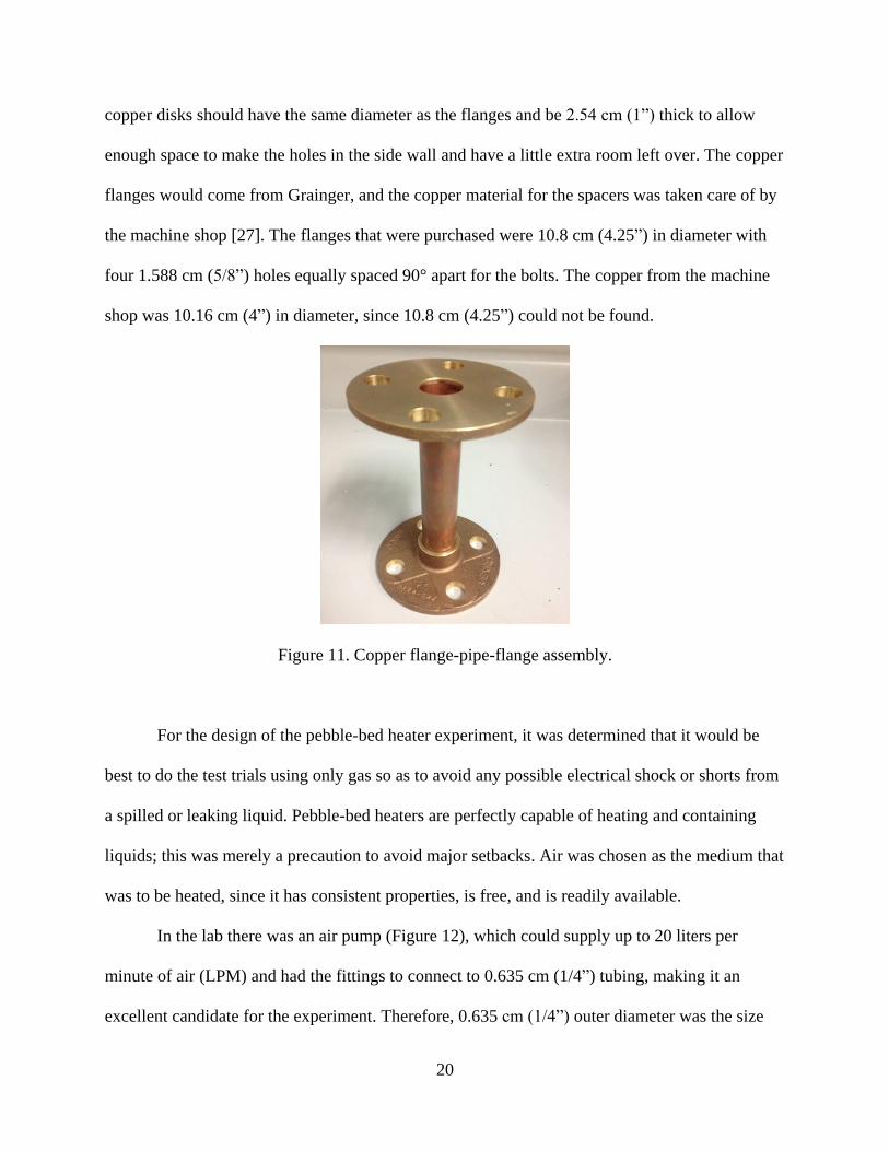
20

copper disks should have the same diameter as the flanges and be 2.54 cm (1”) thick to allow

enough space to make the holes in the side wall and have a little extra room left over. The copper

flanges would come from Grainger, and the copper material for the spacers was taken care of by

the machine shop [27]. The flanges that were purchased were 10.8 cm (4.25”) in diameter with

four 1.588 cm (5/8”) holes equally spaced 90° apart for the bolts. The copper from the machine

shop was 10.16 cm (4”) in diameter, since 10.8 cm (4.25”) could not be found.

Figure 11. Copper flange-pipe-flange assembly.

For the design of the pebble-bed heater experiment, it was determined that it would be

best to do the test trials using only gas so as to avoid any possible electrical shock or shorts from

a spilled or leaking liquid. Pebble-bed heaters are perfectly capable of heating and containing

liquids; this was merely a precaution to avoid major setbacks. Air was chosen as the medium that

was to be heated, since it has consistent properties, is free, and is readily available.

In the lab there was an air pump (Figure 12), which could supply up to 20 liters per

minute of air (LPM) and had the fittings to connect to 0.635 cm (1/4”) tubing, making it an

excellent candidate for the experiment. Therefore, 0.635 cm (1/4”) outer diameter was the size

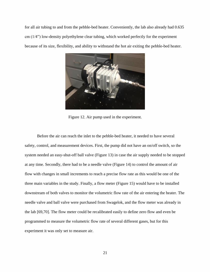
21

for all air tubing to and from the pebble-bed heater. Conveniently, the lab also already had 0.635

cm (1/4”) low-density polyethylene clear tubing, which worked perfectly for the experiment

because of its size, flexibility, and ability to withstand the hot air exiting the pebble-bed heater.

Figure 12. Air pump used in the experiment.

Before the air can reach the inlet to the pebble-bed heater, it needed to have several

safety, control, and measurement devices. First, the pump did not have an on/off switch, so the

system needed an easy-shut-off ball valve (Figure 13) in case the air supply needed to be stopped

at any time. Secondly, there had to be a needle valve (Figure 14) to control the amount of air

flow with changes in small increments to reach a precise flow rate as this would be one of the

three main variables in the study. Finally, a flow meter (Figure 15) would have to be installed

downstream of both valves to monitor the volumetric flow rate of the air entering the heater. The

needle valve and ball valve were purchased from Swagelok, and the flow meter was already in

the lab [69,70]. The flow meter could be recalibrated easily to define zero flow and even be

programmed to measure the volumetric flow rate of several different gases, but for this

experiment it was only set to measure air.

22

Figures 13, 14, 15. Ball valve, needle valve, and flow meter.

For each tubing connection to the air pump, valve, flow meter, or the main device there

would need to be a female fitting that could attach to the tube, secure the tube to its target, and

make an air-tight seal. Swagelok had female 0.635 cm (1/4”) tube fittings that would be screwed

on to the end of each piece of tubing, so that it could mate with any of the previously mentioned

connections. These fittings came in brass and stainless steel, so either brass or stainless steel was

used depending on what metal the particular tube was connecting to.

The air would need to be sent through the heater vertically from bottom to top. For air, if

the flow entered from the top, then the mixed convection would be affected and the net velocity

decreased. The heat escaping the pebbles would rise and slow the flow of the fluid. For liquid, if

the heater was run horizontally, then the liquid would only run through the lower half of the

pebbles. Therefore, the heater would be built vertically with the air entering the base, so that this

device could be experimented with liquids in the future without any modifications.

Now that the air has been supplied, all tubing connected, and the speed regulated, it can

enter the base of the pebble-bed heater. For this connection to exist, another copper disk would

have to be made by the machine shop for the very top and the very bottom of the pebble-bed

heater in order to provide a means of screwing in a fitting on both ends to connect the air tubing

with the heater’s inlet and exit. The fitting on both ends would need a simple 0.635 cm (1/4”)

23

brass male to female fitting. The male side would have NPT (National Pipe Thread) threading so

as to achieve a more air-tight seal against the copper disk, and the other side of the fitting would

be equipped to screw into the 0.635 cm (1/4”) female fitting on the end of the tube. The end disk

would be 2.54 cm (1”) thick and have the 0.635 cm (1/4”) NPT threaded hole cut out on one side

1.27 cm (1/2”) through and then a straight hole would be made the rest of the way. The disk

would also need the four holes 90° apart for the bolts to secure the end piece to the rest of the

device. Figures 16 and 17 show the design of the end disk that the machine shop was to follow

when tooling the copper. The two brass fittings were ordered from Swagelok, and the 10.16 cm

(4”) copper material was purchased by the machine shop [72].

Since the air tubing entering the base had a 0.635 cm (1/4”) diameter, and the pebble

chamber surrounded by the work coil was 2.54 cm (1”), something would have to be added on

the front end of the heater in between the two to normalize the flow and make it more uniform

over the cross-section before the air reached the pebble bed. This addition would need to be

placed after the bottom disk where the air entered and before the first disk containing the two

measuring instruments. To best break up and normalize the flow upon entry, a wad of metal

Figures 16 and 17. The design for the copper end disk spacers.

24

wool (Figure 18) inside a short pipe segment seemed to be the best option. The pipe would again

be 2.54 cm (1”) copper pipe and have a copper flange on either end to connect to both copper

disks. To be consistent, it was decided that there should also be a metal wool pipe segment after

the heating process, so that the air would flow past the second set of instruments in the same way

as the first. The copper pipe and flanges were purchased in the same shipment mentioned

previously, and the bronze wool was found at Home Depot [29]. Since the holes in the flanges

were 1.588 cm (5/8”) in diameter, and there were now four sets of four bolts needed for the

flanges and copper disks; sixteen 1.588 cm (5/8”) diameter, 5.08 cm (2”) long bolts were also

ordered from Home Depot along with the bronze wool from earlier and the nuts to go with the

bolts.

Figure 18. Bronze wool for normalizing the flow of air.

For the steel balls that would make up the pebble matrix, several different sizes would be

considered, since it was decided that the pebble size would be one of the variables in the

experiment. The difference in pebble size would reveal if the volume or surface area of metal

played a role in the exit temperature of the air. First, in order to get more heat out of the steel

25

balls, carbon steel was chosen over stainless steel as the material. Carbon steel and stainless steel

are both comprised of mainly carbon, iron, and several trace amounts of other materials.

However, stainless steel’s iron content is closer to 50%, where as carbon steel can have as much

as 98% iron. Since carbon steel has more iron, it would be more affected by the hysteresis loss

effect. The pipe segment would only be 2.54 cm (1”) wide, so carbon steel balls smaller than

1.27 cm (1/2”) were considered. In order to get a large enough number of pebbles, 0.635 cm

(1/4”), 0.476 cm (3/16”), and 0.318 cm (1/8”) were chosen for the three sizes, and the difference

between the spheres can be seen in figure 19. Carbon steel ball bearings were available in the

desired sizes, so the three sets of ball bearings were purchased from MSC Industrial Supply [40].

As the diameter of the balls decreases, more balls would be needed to fill the same space;

therefore, the number of ball bearings which was ordered increased as the diameter decreased:

500 of the 0.635 cm (1/4"), 1000 of the 0.476 cm (3/16”), and 2,500 of the 0.318 cm (1/8”).

Figure 19. Carbon steel ball bearings: 0.635 cm (1/4"), 0.476 cm (3/16”), 0.318 cm (1/8”).

Once the steel ball selection had been made, it was decided that there would have to be a

wire grate or wire mesh before and after each segment to prevent the steel balls and even the

wire wool from moving between the sections of the pebble-bed heater. The wire mesh would still

26

allow the air to flow through unobstructed. It had to be strong enough to support the weight of

the pebbles and have small enough holes so that the 0.318 cm (1/8”) balls could not slip through.

After searching several stores, some aluminum wire mesh (Figure 20) was found at Hobby

Lobby with 0.159 cm (1/16”) holes that were small enough to not let anything but air pass

through [28].

Two thermocouples would be needed for the experiment; one above and one below the

pebble matrix. As mentioned previously, the thermocouples would come in through the side of

the middle copper spacers and be held by brass fittings. Thermocouples come in several different

models or “types”; each type is capable of reading different temperature ranges and serving

Figure 20. Aluminum wire mesh with 0.159 cm (1/16”) holes.

unique functions. Originally, K-type was considered, since it had the most favorable temperature

range for the experiment, capable of reading up to 1,523 K (2,282 °F). Once it was learned that

K-type thermocouples did not function inside magnetic fields, they could no longer be used [50].

Instead, T-type thermocouples (Figure 21) were found to be a suitable substitute. T-type could

only read up to 623 K (662 °F) but were unaffected by magnetic fields, so they were the best

option for the small-scale testing in which temperatures were not going to be close to the

maximum reading temperature [50]. Using Omega’s selection guide to choose the proper

27

thermocouple, two T-type thermocouples were purchased [51]. In order to reach the center of the

air flow, the thermocouple should have at least a 15.24 cm (6”) long probe. The two

thermocouple fittings would come from Swagelok. The fittings needed male NPT threading on

one end to securely fasten to the copper disk, a female connection on the other end to secure the

thermocouple, and the interior to be “bored through” so that the thermocouple could pass

through the fitting [71].

Figure 21. T-type thermocouple with 15.24 cm (6”) probe.

In order to read the temperature value from the thermocouple, the millivolts could be read

from the two wires coming out of the instrument using a digital multimeter (DMM). The voltage

would then be converted to a temperature using the T-type thermocouple reference tables [52].

The thermocouple’s wires could also simply be hooked up to a thermocouple reader, which

would take care of all conversions and display the temperature value. To avoid the hassle, time,

and potential error from the conversion technique, the thermocouple reader method was chosen.

The lab owned several thermocouple readers with different capabilities. The reader selected for

the experiment, which can be seen in figure 22, had the ability to measure up to 10

thermocouples, read different “types” of thermocouples, and calibrate using an ice bath.

28

Figure 22. Thermocouple reader.

In addition to temperature, the pressure difference was also to be measured. To

accomplish this, a differential pressure transducer (DPT) was to be used. The lab owned the DPT

in figure 23, which was capable of measuring changes in air pressure. It had a port on either end

to which a pipe or tube could be attached. This DPT would need to have some of the 0.635 cm

(1/4") low-density polyethylene clear air tubing attached to each of the two ports—one to

measure the higher pressure and one for the lower. The lower temperature port would connect to

the spacer before the heating, and the higher temperature port would connect to the spacer after

the heating, since the pressure would increase as temperature increased. At each connection to a

spacer, there would be another bored-through, male NPT threaded fitting to allow the tubing to

pass through the fitting and read from the middle of the flow [73]. In order to read the difference

in pressure, a digital multimeter would have to clip onto the two output wires of the DPT. Next,

the displayed voltage on the multimeter would be converted to difference in pressure in units of

Pascals (Pa=N/m2) using equation 3, which was derived from the instrument’s user manual [49].

[ ] [

] [ ] Eq. 3

29

Figure 23. Differential pressure transducer with DMM clips attached to output.

After both the pebble-bed heater and induction heater had been built, an issue arose with

the copper pipe center section. The induction heater would short out every time the copper work

coil touched the copper pipe or any metal object. To resolve this insulation problem, the pebble

chamber and its two flanges would no longer be made out of copper and instead were designed

as one solid unit in Solidworks as seen in figure 24. Proper thickness was given to the pipe walls,

so the material was sturdy and strong enough to support the load of weight above it. The design

of the printed piece would be the exact same dimensions as the copper version, except that it

would be made as one solid piece to minimize the possibility of air leaks and weak points. Three

of these units were successfully printed using ABS plastic material at The University of

Alabama’s 3D Printing Lab. The main disadvantage of the ABS plastic is that it transitions from

a hard plastic to a rubbery plastic at 377 K (219 °F), which means that high temperatures cannot

be achieved with this part as the pebble chamber [68]. This was intended to be a temporary fix,

so that experiments could be run, not a permanent solution to the magnetic induction pebble-bed

heater. The permanent solution is covered in the Discussion section later in this paper.

30

Figure 24. Solidworks drawing of pipe and flange assembly.

Finally, after designing and giving careful consideration to each aspect of the pebble-bed

heater and having acquired all the parts and tools necessary, the construction of the pebble-bed

heater could begin. The pneumatic schematic of the system can be seen in figure 25.

Figure 25. Schematic of the pebble-bed heater experiment.

B) Constructing the Pebble-Bed Heater

Before construction could begin, the two copper flange-pipe-flange sections for the wire

wool needed to be sweated together by The University of Alabama’s machine shop. The

sweating process would not only secure the pipe to the two flanges, but it would also make the

connection air-tight.

31

For the next step of the preparation process, the aluminum mesh was cut to make six

different circles that were slightly larger than the 2.54 cm (1”) hole. Then, six cardboard cutouts

had to be made. The cardboard would act as a washer preventing air from leaking out of the gap

made by the thin wire mesh as well as a means of securing the aluminum mesh circles to the

different parts of the assembly. The cardboard was cut the same way as the flange. It had a 2.54

cm (1”) hole in the center, 10.8 cm (4.25”) outer diameter, and four equidistant 1.588 cm (5/8”)

holes for the bolts. Using cyanoacrylate (Krazy Glue), each piece of aluminum mesh was

adhered over the center hole in each of the cardboard cutouts.

With all parts in hand and all preparation work finished, the heater construction began at

the start with the air pump. The air pump did not require any assembly or wiring, but it did need

to be secured to the table, since it would vibrate and move while turned on. The air pump had

holes in its legs that would allow it to be screwed down; however, the spacing of the screw holes

did not fit with the table that the experiment was being conducted on. Therefore, the air pump

was kept in place by putting tape underneath it.

Seven pieces of air tubing were then cut and female fittings secured to each end. Three

short pieces were cut to be less than 15.24 cm (6”) long, three medium pieces were cut to be

about 30.48 cm (1’) long, and one long segment was made to be almost 60.96 cm (2’) long. With

the first short piece, one end was tightened onto the air pump’s exit, and the other was attached

to the ball valve. Plumbing tape was used on every fitting connection in the entire setup to ensure

that air could not easily escape through the grooves. Another short piece of tubing was placed

between the ball valve and the needle valve, and the third was fastened between the needle valve

and the flow meter. The long cut of tubing connected the flow meter to the fitting at the base

entrance of the pebble-bed heater. Finally, a piece of padding was placed under the ball valve

32

and needle valve to reduce vibration noise caused by the air pump. Figure 26 shows the entire

initial configuration prior to the pebble-bed heater.

Figure 26. Experiment configuration from air pump to flow meter.

The fitting at the base was screwed into the NPT threaded hole on the underside of the

bottom copper disk. Next, the copper pipe with the metal wool was to be installed to help make

the flow uniform. A small wad of the bronze wool was stuffed inside one of the small flange-

pipe-flange sections but not compacted enough to restrict airflow. A piece of aluminum mesh

and cardboard was adhered to the outer side of each flange preventing the wool from interfering

with other parts of the heater. One of the flanges was then secured to the copper base using four

of the bolts. The progress can be seen in figure 27.

Figure 27. Construction up to the first pipe section.

33

Next, the first middle copper spacer would be installed. In addition to simply being

placed atop the flange, the first thermocouple probe and low-pressure DPT tube needed to be

installed in the side. After being wrapped with plumbing tape, the thermocouple and tube fittings

were tightened into the side wall. The thermocouple probe was pushed through the fitting and

fastened to the fitting once the probe was in the center of the inner 2.54 cm (1”) hole. The same

process was done for the DPT tubing after two of the medium length tubing sections were fixed

to either port on the DPT. Both fittings are shown in figures 28 and 29.

Figures 28 and 29. Thermocouple probe and DPT tube attached to the copper spacer.

After everything had been attached to the first disk, the 3D-printed, ABS plastic center

section would follow. Another aluminum mesh and cardboard part was glued to the base of the

plastic pipe, so that the ball bearings would not fall out of the bottom. The first set of ball

bearings loaded into the pebble chamber was the 0.635 cm (1/4”) carbon steel balls. The ball

bearings were counted as they were loaded into the pipe, and it took 300 of the 0.635 cm (1/4")

size to fill the 15.24 cm (6”) long pipe. Once full, the chamber was bolted to the disk and bronze

wool pipe section below. Figure 30 shows the development of the experiment up until this stage.

34

Figure 30. Construction up to the main center chamber.

The fourth cardboard cutout was then attached to the under-side of the second copper

disk instead of the top of the 3D printed pipe, so that the ball bearings could be emptied and

filled. The two fittings were tightened into the second middle disk, and then the second

thermocouple probe and high-pressure DPT tube were attached in the same way as before in

order to read from the middle of the 2.54 cm (1”) hole where the air would be flowing.

The second wad of bronze wool was stuffed inside the remaining short copper pipe, and

then the last two cardboard and aluminum mesh pieces were adhered to the outer side of each

flange to contain the bronze wool. One of the copper flanges was then bolted to the copper disk

and plastic flange.

For the final part of the main pebble-bed heater construction process, the second outer

copper disk was placed atop the remaining flange, and the last set of four bolts tightened them

together. A 0.635 cm (1/4") tube fitting with NPT threads was screwed into the hole on the top of

the disk, so that the third medium length piece of air tubing that was cut in the beginning could

be attached to the exit of the pebble-bed heater. The exit hose was necessary, so that hot air was

not leaving the system in an uncontrolled manner. The air could now be directed to a safe area.

35

In the event that a liquid is used instead of a gas in future testing, this would also provide a

means of depositing the liquid into a bucket or sink.

Once the heater was finished being built, it needed a way to stand vertically and not be

knocked over easily. The lab had a large collection of extruded aluminum frame pieces and

connectors, so a stand would be made out of that to hold the heater vertically [80]. The rods are

square 2.54 cm (1”) by 2.54 cm (1”) rods of various lengths. The pieces can be attached to each

other easily in any direction using only the supplied joints, fasteners, and an allen wrench

making it ideal for creating a customized stand. The base of the heater needed to be about 5.08

cm (2”) off of the ground, so that the air tube and fitting would have enough room to come up

and enter the bottom. The rods were spread wide at the base to prevent tipping. Then, a second

layer perpendicular to the first was set closer to the center for the heater to rest on. The gap

between the two rods was barely wide enough for the bolts at the base to fit between. A third

layer was set perpendicular to the second layer—parallel to the first—with the rods 10.16 cm

(4”) apart, so that the device would have a very tight fit to keep it from wobbling. Then, several

longer rods were stood vertically at the four corners and connected to one another, so that the

pebble-bed heater could not easily be hit and knocked over. The vertical stand and pebble-bed

heater were now complete as seen in figure 31 with only a few minor steps left.

In addition to the main construction, the thermocouple reader and differential pressure

transducer needed to be set up. The thermocouple reader had the ability to measure up to 10

different probes, so there were 10 locations for thermocouples to attach in the rear. The two

copper-constantan thermocouple wires were screwed into the first two ports of the device as seen

in figure 32. The #1 thermocouple was the upstream probe before the matrix, and the #2

36

Figure 31. Completed stand and pebble-bed heater.

thermocouple was the probe after the heating had taken place. Once the instruments were

connected to the machine, the probes were submerged in an ice bath for ten minutes in order to

calibrate the device to 273 K (32 °F). After calibration, the probes were reconnected to their

respective places in the pebble-bed heater.

Figure 32. Rear of thermocouple reader with thermocouples connected to ports 1 and 2.

37

The differential pressure transducer required some wiring before it could be used. The lid

was unscrewed, and a 250 ohm resistor was added between terminals 2 and 3 as shown in figures

33 and 34, so that the device would output the pressure reading in volts instead of amps. The 250

ohms was reached using four 100 ohm resistors in a combination of series and parallel. To

calibrate the DPT, both the high pressure and low pressure ends were stopped up, so the pressure

would be the same on either end with no velocity or temperature difference. Once the pressure

difference was zero, the calibration potentiometer on the far left side of the DPT was twisted

until the output read 1 volt (1 V = 0 Pa, see equation 3). The lid was re-attached, and the tubes

were placed back inside the heater.

A complete step-by-step process of the construction is pictured in the Appendix. The

pebble-bed heater portion of construction was now fully complete, and the induction heater

design process could begin.

Figures 33 and 34. The internal wiring and wiring diagram of the DPT.

C) Designing the Induction Heater

The design of the magnetic induction heater in the experiment began with finding a

practical schematic. The wiring design had to be powerful enough to provide the necessary heat,

250 ohm resistor

Calibration Potentiometer

38

but not so complex that it could not be easily reproduced. The schematic chosen for the pebble-

bed heater would come from www.RMCybernetics.com [61]. The design was very simple yet

powerful and only required nine main parts along with a power supply unit. The schematic was

modified to add more detail and can be seen in figure 35. This circuit is called a collector

resonance oscillator circuit. It is both simple and self-resonating, so it will automatically run at

the resonant frequency determined by the capacitors and work coil [61]. While this circuit was

practical for a small-scale, low temperature test, it would not be suitable for a bigger scale with

larger amounts of metal or if a temperature above 533 K (500 °F) was desired.

Figure 35. Schematic of the induction heater used in this experiment.

The first major component was a DC power supply unit. The power supply needed to be

capable of providing up to 15 volts and 5 amps and delivering a large surge of current at start up.

In addition, the voltage and current level had to be easily adjustable, since the amount of power

delivered to the coil would be the third variable in this study. There were a number of available

power supply units in the lab. Although, several devices were incapable of being adjusted, some

39

lacked a display, and others did not deliver a high enough voltage. The one shown in figure 36

was capable of meeting all the needs and therefore chosen for the experiment.

The next aspect of the design process was determining the specific electrical components

necessary to create the induction heater as these details were not included in the original

schematic. The parts included a work coil, a choke inductor, six capacitors, two resistors, two

diodes, and two transistors.

Figure 36. DC power supply with electronic display and adjustable voltage.

The coil for this schematic was required to be a solenoid with a center tap—a location for

current to enter at the middle of the solenoid. Different coils were considered and tested to find

the best fit. The solenoid would need to be made of a conductive material that was thick enough

to handle the large amounts of current. This meant that the coil could either be a thick wire or a

small pipe, and the material would be brass or copper. Brass was dismissed once it was found to

deform at high temperatures, which meant copper was to be the solenoid material [61]. Soft

copper pipe worked quite well as a work coil. It was easy enough to bend and wind into shape so

40

that it had the desired inner diameter to fit around the pipe. The pipe was able to withstand high

frequency currents better than a wire, as the current would flow around the outside of the pipe

instead of building up a resistance. If cool water was run through the center of the pipe, then it

could tolerate even higher power levels and temperatures.

Unfortunately, the only soft copper pipe found was uninsulated and the circuit would

short if any metal touched the coil, so a thick, insulated, copper wire was the final solution.

While the wire would be thinner than the pipe and unable to carry as high of a current, it would

allow the solenoid to have more turns per unit length, which would increase the density of the

magnetic field. Using a wire selection guide, gauge 12 wire was chosen, since it could handle the

5 amp current for a longer distance than was necessary and was still easy enough to bend into

shape [23]. The gauge 12, copper, solid-core wire for the solenoid was cut in a 6.096 m (20’)

long segment from the lab.

The current would first be supplied to the solenoid at its center, but before the current

could reach the center tap of the solenoid, it must pass through an inductor, referred to as a

“choke inductor.” Choke inductors range from less than one microhenry (µH) to several hundred

millihenries. Its purposes include preventing the high frequency oscillations from entering the

power supply and keeping the current at a reasonable level [61]. The choke inductor will

therefore increase the lifespan of the system and reduce maintenance. Just like the work coil, the

choke inductor would need to be made of a thick enough gauge wire to handle the high levels of

current being supplied to the solenoid. Another factor to consider is that in an induction heater

system, the choke inductor needs to have a reasonably high inductance of several hundred

microhenries to block the high frequency oscillations, so a 500 µH choke inductor made of thick

wire was purchased from Mouser Electronics and can be seen in figure 37 [39].

41

Figure 37. 500 µH choke inductor.

Looking at the schematic, there is a capacitor in parallel with the work coil creating a

resonant tank circuit thus generating a resonant frequency within the system. Instead of having

one large capacitor, it would be better to distribute the current and heat among more capacitors,

so that, as a whole, the capacitors could handle a higher power level and be less likely to fail.

Therefore, six 330 nanofarad (nF) capacitors were combined in parallel to each other and with

the solenoid to reach 1.98 microfarads, which would reduce the resonant frequency to a safe

level (21.74 kHz) according to RMCybernetics [61]. After searching online, 1 kV, 330 nF,

polypropylene capacitors were found from Digikey (Figure 38) [13].

Figure 38. Six 330 nF capacitors combined in parallel with each other and the work coil.

42

The voltage and current also enter the circuit through two resistors. Their resistance

determines how quickly the transistors will turn on and should therefore be a relatively low

amount. Although, if the resistance is too low, the resistor would be pulled to ground by the

diode when the opposite transistor is active, so the resistance should be lower than 500 ohms but

not below 100 ohms [61]. 240 ohms was determined to be a safe value, and the appropriate

resistors were purchased from www.RMCybernetics.com [62].

The two diodes in the circuit are responsible for discharging a transistor, while the other

transistor is activated. In order to drain the transistor quickly and completely, the diode selected

should have a low forward voltage drop and a quick response time. The diode should also be able

to handle high surges of voltage and prevent a reverse flow of voltage. Schottky diodes were

considered, since they are known for having a low forward voltage drop and rapid switching

speed [24]. More specifically though, a Schottky rectifier diode was chosen for the circuit, since

it was better equipped to prevent reverse voltage flow than a standard Schottky diode [24]. The

rectifier diodes were purchased from Digikey [11].

The final electrical element to the circuit was the transistors. The two transistors would

be activated by their resistors and drained by the diodes, and the transistors themselves would be

responsible for alternating the flow direction of current in the work coil. The specific transistor

model chosen would need to be capable of functioning at the frequency determined by the

capacitors and be rated for at least five times the voltage and current that the circuit will be

supplied with. MOSFETs (Metal-Oxide Semiconductor Field-Effect Transistor) were chosen due

to their low drain-source resistance and fast response time [74]. This would allow them to both

drain and turn on/off quickly. A large number of these transistors would need to be ordered,

43

since they are the piece that short circuits easily. They would burn up if anything was wrong with

the circuit or if any metal touched an uninsulated part of the work coil. The transistors can also

decline in performance after twenty to thirty hours of use and would eventually need to be

replaced. The MOSFETs were ordered from Digikey along with the diodes and capacitors [12].

Since the MOSFETs were likely to get warm during testing due to the long tests and the

high operating frequency, it was necessary to get a heat sink for each transistor. The transistors

had a hole in them for a small screw, so the heat sinks needed to have a small hole of the same

size. As shown in figure 39, this would hold the transistor to the heat sink for a good connection,

allowing the heat to easily transition to the heat sink. A suitable heat sink was found on Digikey,

and one was purchased for each transistor [14].

Figure 39. MOSFET and heat sink.

Typically, a solderless breadboard would be used to hold the circuit and connect the

pieces to one another. Since the circuit would be using up to 5 amps and the lab only had

breadboards capable of handling up to 1 amp, the circuit would have to be built as a floating

circuit. This meant that the wires, resistors, diodes, etc. would not be plugged into anything. The

44

wires would simply be twisted or soldered to one another. To make the floating circuit somewhat

more secure, 10 amp alligator clips and several plastic twist nuts were used to help with

connections.

D) Constructing the Induction Heater

The work coil took several attempts before a suitable center-tapped solenoid was made.

The first efforts involved a 0.847 cm (1/3”) soft copper pipe and then the 12 gauge wire. The first

attempt with the pipe was a failure, but the second solenoid was made as one solid unit and

several turns longer than the first. The pipe was easy enough to bend into shape around the outer

diameter of the pebble chamber. The wire connecting the solenoid to the choke inductor could

either wrap around a point at the center of the coil or be soldered to the same point. Soldering

was not as easy on the pipe, so a ring of solder was made around the pipe. Next, the wire from

the choke inductor was inserted into the solder. The end result, seen in figure 40, was a success

and would have been used in the final experiment if it had been better insulated. If the copper

coil ever touched a piece of metal while the power supply was on, the transistors would burn up

and need to be replaced.

Figure 40. Solenoid made from copper pipe.

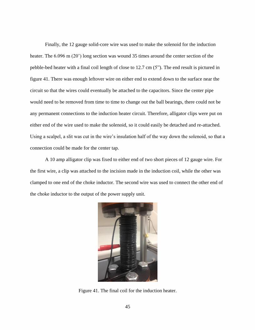
45

Finally, the 12 gauge solid-core wire was used to make the solenoid for the induction

heater. The 6.096 m (20’) long section was wound 35 times around the center section of the

pebble-bed heater with a final coil length of close to 12.7 cm (5”). The end result is pictured in

figure 41. There was enough leftover wire on either end to extend down to the surface near the

circuit so that the wires could eventually be attached to the capacitors. Since the center pipe

would need to be removed from time to time to change out the ball bearings, there could not be

any permanent connections to the induction heater circuit. Therefore, alligator clips were put on

either end of the wire used to make the solenoid, so it could easily be detached and re-attached.

Using a scalpel, a slit was cut in the wire’s insulation half of the way down the solenoid, so that a

connection could be made for the center tap.

A 10 amp alligator clip was fixed to either end of two short pieces of 12 gauge wire. For

the first wire, a clip was attached to the incision made in the induction coil, while the other was

clamped to one end of the choke inductor. The second wire was used to connect the other end of

the choke inductor to the output of the power supply unit.

Figure 41. The final coil for the induction heater.

46

The next step was to install the capacitors. For best results, the capacitors should be

placed as close as possible to the solenoid. In order to secure each of the six capacitors to either

end of the coil’s wire, a short segment of 12 gauge, multi-strand wire was used. Since the wire

was multi-stranded, the legs of the capacitors could easily be run directly through the middle of

the wire, wrapped around, and soldered for a permanent connection. This was done for each of

the capacitors until all six were in parallel. In order to give the clips from the solenoid a good

grasp on the multi-strand wire, the end of both multi-strand wires going to the coil were covered

in soldered. Alligator clips were attached to the other ends of the wires going towards the circuit.

Before the circuit could be built, some research into MOSFETs had to be conducted. The

MOSFETs had three legs called the gate, source, and drain. If looking from the front side, the

gate was on the left, drain in the middle, and the source on the right for the particular MOSFETs

purchased [66]. If the transistor was “On,” then the voltage would enter the gate, opening a

connection between the drain and source. This connection would provide a pathway for the

voltage from the work coil and the voltage intended for the “Off” transistor to be grounded [74].

The transistors would then flip roles; the transistor that was “Off” was now “On” and vice versa.

This would cause the opposite transistor to act as the ground for the work coil compared to

before reversing the direction of the current and the magnetic field. This process would happen

as many times per second as the frequency of the resonant tank circuit.

Before any wiring took place, the MOSFETs were first fixed to their heat sinks using a

small screw and nut. A wire was then soldered to each of the three legs to give it additional

length. A cable was run from the output of the power supply to a wire, which was connected to

the two resistors by a twist nut. The other end of each resistor was then connected to both the

47

upstream side of a diode and the gate of a MOSFET using a twist nut. The downstream side of

each diode was then connected to the drain of the opposite MOSFET. The source legs of each

MOSFET were connected to each other with a twist nut and then connected to the ground of the

power supply by a cable. Finally, an alligator clip coming from each capacitor wire was clamped

to the downstream side of one of the diodes. Without a breadboard and with so many junctions,

the end result of the circuit was a bit clustered, as seen in figures 42 and 43, but functioned

perfectly.

Figures 42 and 43. Induction heater circuit and wiring.

To verify that the induction heater was functioning, a screw driver was inserted inside the

solenoid for 30 seconds. After removing the screwdriver, the temperature was measured using an

infrared thermometer, and it was found to be over 366 K (200 °F). A paper clip was then entered

into the same magnetic field was close to 478 K (400 °F) after the time period. This simple test

proved that the induction heater indeed worked.

48

CHAPTER 4

TESTING PROCEDURE

As mentioned previously, the experiment of the small-scale magnetic induction pebble-

bed heater would be subjected to numerous tests involving different combinations of pebble

sizes, flow rates, and power levels. There would be tests run at three different voltages, flow

rates, and pebble sizes with every combination possible. Therefore, 27 total experiments would

be conducted, and they would be completed in sets of three to minimize strain on the system. To

reduce the time between tests, the pebble size would only be changed after the 9 tests with the

current pebble size had been run. The reason being, it would take more time to change the pebble

size than it would to adjust the knobs and valves for the power supply and flow rate. The three

pebble sizes were 0.635 cm (1/4"), 0.476 cm (3/16”), and 0.318 cm (1/8”). In order to avoid

reaching high temperatures that would melt the plastic pebble chamber, 10 volts would be the

highest voltage applied to the system. The three voltage levels would be 5, 7.5, and 10 volts. The

air pump had a maximum flow rate of 20 liters per minute (LPM), so the flow rates would be 10,

15, and 20 LPM. During a performance test with the air pump, the max flow rate from the air

pump would drop about 2-3 LPM after an hour of testing. Consequently, the higher flow rates

were always tested first.

The first set of ball bearings would be the 0.635 cm (1/4”) diameter set. After filling the

pebble chamber to the brim, it was found that 300 of the balls could fit inside. Once loaded, the

pebble-bed heater was bolted back together. Prior to each test session, the air pump and

induction heater would be shut off, so the DPT and flow meter could be set to zero in order to

improve the accuracy of the results.

49

The first set of three experiments would be run at 20 LPM, and the three different voltage

levels would be applied in increasing amount. By increasing the voltage between tests instead of

decreasing, it would eliminate unnecessary time waiting for the system to cool back down. Once

the max temperature was reached at the first voltage, the voltage would be increased to the

second level, and the temperature would rise from the end of the previous test. The same would

be done for the third voltage. The current provided to the circuit was automatically adjusted by

the circuit and the power supply. The current was dependent on the surface area of metal inside

the solenoid and the voltage level. Equation 4 shows the voltage-current relationship for the

0.635 cm (1/4”) carbon steel balls as determined by the linear relationship in figure 44, accurate

to within 0.05 amps.

[ ] [

] [ ]

Figure 44. Voltage-current relationship for 0.635 cm (1/4”) balls.

At 20 LPM the air would reach 90% of the maximum temperature after 10 minutes, but it

would take approximately 20 total minutes before the exit temperature of the air would stop

Eq. 4

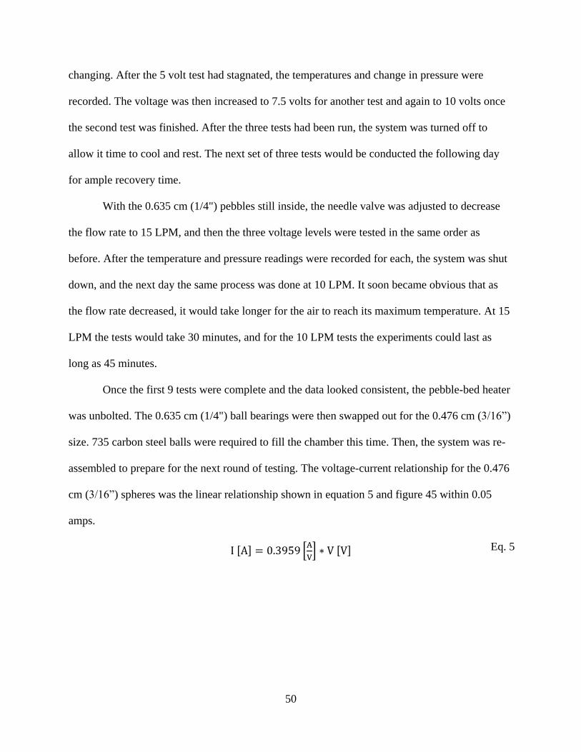
50

changing. After the 5 volt test had stagnated, the temperatures and change in pressure were

recorded. The voltage was then increased to 7.5 volts for another test and again to 10 volts once

the second test was finished. After the three tests had been run, the system was turned off to

allow it time to cool and rest. The next set of three tests would be conducted the following day

for ample recovery time.

With the 0.635 cm (1/4") pebbles still inside, the needle valve was adjusted to decrease

the flow rate to 15 LPM, and then the three voltage levels were tested in the same order as

before. After the temperature and pressure readings were recorded for each, the system was shut

down, and the next day the same process was done at 10 LPM. It soon became obvious that as

the flow rate decreased, it would take longer for the air to reach its maximum temperature. At 15

LPM the tests would take 30 minutes, and for the 10 LPM tests the experiments could last as

long as 45 minutes.

Once the first 9 tests were complete and the data looked consistent, the pebble-bed heater

was unbolted. The 0.635 cm (1/4") ball bearings were then swapped out for the 0.476 cm (3/16”)

size. 735 carbon steel balls were required to fill the chamber this time. Then, the system was re-

assembled to prepare for the next round of testing. The voltage-current relationship for the 0.476

cm (3/16”) spheres was the linear relationship shown in equation 5 and figure 45 within 0.05

amps.

[ ] [

] [ ] Eq. 5

51

Figure 45. Voltage-current relationship for 0.476 cm (3/16”) balls.

With the 0.476 cm (3/16”) pebbles, testing was conducted in the same manner as with the

0.635 cm (1/4”) pebbles. The 20 LPM test set was performed first for each of the three power

levels, the three 15 LPM tests the following day, and the final set at 10 LPM the day after that.

Once the second set of 9 tests had been run and produced reasonable results, the 0.476 cm

(3/16”) spheres were changed out for the smaller 0.318 cm (1/8”) size. 2,500 of these balls were

needed to fill the center section. Once the pebble-bed heater was re-constructed, the new current-

voltage relationship was found to be equation 6 from figure 46.

[ ] [

] [ ]

y = 0.3959x R² = 0.9984

1.50

2.00

2.50

3.00

3.50

4.00

5 6 7 8 9 10

Cu

rre

nt

[A]

Voltage [V]

Voltage vs Current (3/16" pebbles)

Eq. 6

52

Figure 46. Voltage-current relationship for 0.0.318 cm (1/8”) balls.

The same testing procedure was followed for this group of 9 tests as the 0.635 cm (1/4”)

and 0.476 cm (3/16”) experiments. After three more days, the remaining 9 data sets of

temperature and pressure values were recorded, and then all 27 tests had been completed. Now

that all testing had concluded, the data could be observed and analyzed to search for the behavior

of a pebble-bed heater powered by magnetic induction and for a relationship between the

Dimensionless Heat Transfer, Dimensionless Power, and Reynolds number.

53

CHAPTER 5

RESULTS

The experiment data from each of the 27 tests was recorded in an organized and easy to

read table (Table 1). The table shows how the maximum temperature would increase and

decrease under the different variable combinations. The pebble-bed heater hardly had an effect

on the pressure with the largest pressure increase being less than 650 Pa (0.1 psi); therefore,

pressure will be left out of this analysis and considered to be constant.

Table 1. Temperature data from all 27 tests in °F, °C, and K.

In short, the exit temperature would increase if the voltage/power applied to the system

increased as seen in figures 47-49, since a greater current would be induced, and the magnetic

field would be stronger. The error bars were not included in the plots, since the uncertainty was

Pebble D Flow Rate

[in] [LPM]

1/8 20

1/8 20

1/8 20

1/8 15

1/8 15

1/8 15

1/8 10

1/8 10

1/8 10

3/16 20

3/16 20

3/16 20

3/16 15

3/16 15

3/16 15

3/16 10

3/16 10

3/16 10

1/4 20

1/4 20

1/4 20

1/4 15

1/4 15

1/4 15

1/4 10

1/4 10

1/4 10

Current Voltage Power Tempin Tempout Tempin Tempout Tempin Tempout ΔT ΔT

[A] [V] [W] [F] [F] [C] [C] [K] [K] [F] [K]

3.34 10 33.4 75.7 162.4 24.3 72.4 297.4 345.6 86.7 48.2

2.49 7.5 18.7 74.4 120.8 23.6 49.3 296.7 322.5 46.4 25.8

1.64 5 8.2 73.0 93.2 22.8 34.0 295.9 307.2 20.2 11.2

3.34 10 33.4 76.8 182.7 24.9 83.7 298.0 356.9 105.9 58.8

2.49 7.5 18.7 76.6 137.6 24.8 58.7 297.9 331.8 61.0 33.9

1.64 5 8.2 76.8 102.6 24.9 39.2 298.0 312.4 25.8 14.3

3.34 10 33.4 74.7 203.4 23.7 95.2 296.9 368.4 128.7 71.5

2.49 7.5 18.7 73.6 148.2 23.1 64.6 296.3 337.7 74.6 41.4

1.64 5 8.2 73.5 105.5 23.1 40.8 296.2 314.0 32.0 17.8

3.99 10 39.9 73.8 166.4 23.2 74.7 296.4 347.8 92.6 51.4

2.96 7.5 22.2 72.9 124.5 22.7 51.4 295.9 324.5 51.6 28.7

1.94 5 9.7 72.5 96.4 22.5 35.8 295.7 308.9 23.9 13.3

3.99 10 39.9 72.8 189.2 22.7 87.3 295.8 360.5 116.4 64.7

2.96 7.5 22.2 72.5 139.6 22.5 59.8 295.7 332.9 67.1 37.3

1.94 5 9.7 72.1 105.8 22.3 41.0 295.4 314.2 33.7 18.7

3.99 10 39.9 75.6 214.1 24.2 101.2 297.4 374.3 138.5 76.9

2.96 7.5 22.2 75.6 160.4 24.2 71.3 297.4 344.5 84.8 47.1

1.94 5 9.7 75.6 115.6 24.2 46.4 297.4 319.6 40.0 22.2

4.43 10 44.3 73.4 188.7 23.0 87.1 296.2 360.2 115.3 64.1

3.28 7.5 24.6 72.8 140.2 22.7 60.1 295.8 333.3 67.4 37.4

2.14 5 10.7 72.4 107.2 22.4 41.8 295.6 314.9 34.8 19.3

4.43 10 44.3 73.2 212.2 22.9 100.1 296.0 373.3 139.0 77.2

3.28 7.5 24.6 72.7 157.5 22.6 69.7 295.8 342.9 84.8 47.1

2.14 5 10.7 72.2 117.2 22.3 47.3 295.5 320.5 45.0 25.0

4.43 10 44.3 73.2 233.0 22.9 111.7 296.0 384.8 159.8 88.8

3.28 7.5 24.6 72.8 176.3 22.7 80.2 295.8 353.3 103.5 57.5

2.14 5 10.7 72.3 132.1 22.4 55.6 295.5 328.8 59.8 33.2

54

only +/- 0.1571 K (+/- 0.2828 °F). Except for the 10 LPM test with the 0.635 cm (1/4”) ball

bearings, the trendline equations are more than 96% accurate.

Figure 47. Temperature change vs power supplied at fixed flow rate for 0.635 cm (1/4") balls.

Figure 48. Temperature change vs power supplied at fixed flow rate for 0.476 cm (3/16") balls.

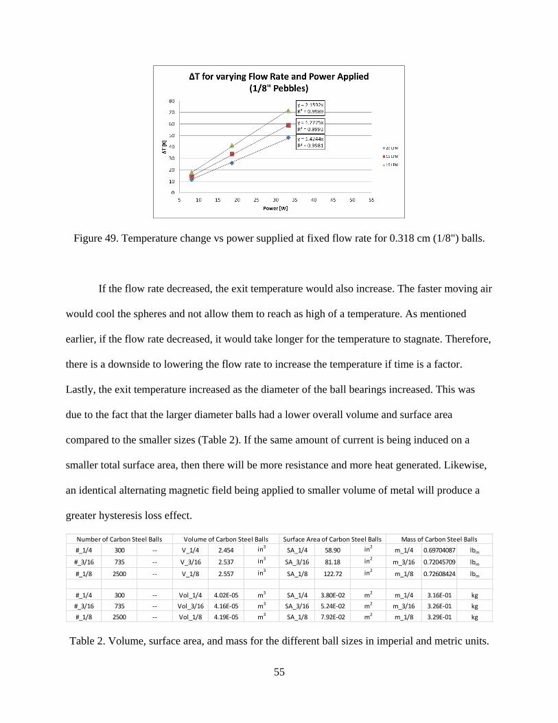
55

Figure 49. Temperature change vs power supplied at fixed flow rate for 0.318 cm (1/8") balls.

If the flow rate decreased, the exit temperature would also increase. The faster moving air

would cool the spheres and not allow them to reach as high of a temperature. As mentioned

earlier, if the flow rate decreased, it would take longer for the temperature to stagnate. Therefore,

there is a downside to lowering the flow rate to increase the temperature if time is a factor.

Lastly, the exit temperature increased as the diameter of the ball bearings increased. This was

due to the fact that the larger diameter balls had a lower overall volume and surface area

compared to the smaller sizes (Table 2). If the same amount of current is being induced on a

smaller total surface area, then there will be more resistance and more heat generated. Likewise,

an identical alternating magnetic field being applied to smaller volume of metal will produce a

greater hysteresis loss effect.

Table 2. Volume, surface area, and mass for the different ball sizes in imperial and metric units.

#_1/4 300 -- V_1/4 2.454 in3SA_1/4 58.90 in2

m_1/4 0.69704087 lbm

#_3/16 735 -- V_3/16 2.537 in3SA_3/16 81.18 in2

m_3/16 0.72045709 lbm

#_1/8 2500 -- V_1/8 2.557 in3SA_1/8 122.72 in2

m_1/8 0.72608424 lbm

#_1/4 300 -- Vol_1/4 4.02E-05 m3 SA_1/4 3.80E-02 m2 m_1/4 3.16E-01 kg

#_3/16 735 -- Vol_3/16 4.16E-05 m3 SA_3/16 5.24E-02 m2 m_3/16 3.26E-01 kg

#_1/8 2500 -- Vol_1/8 4.19E-05 m3 SA_1/8 7.92E-02 m2 m_1/8 3.29E-01 kg

Number of Carbon Steel Balls Volume of Carbon Steel Balls Surface Area of Carbon Steel Balls Mass of Carbon Steel Balls

56

In order to convert the results into dimensionless form, several air properties had to be

found first: density, specific heat, thermal conductivity, and kinematic viscosity. Since each

property was dependent on temperature, the same value could not be used for every test. The

temperature used to determine the exact density, specific heat, conductivity, or viscosity was the

exit temperature of the air for each test [16,17,18]. The temperature dependent value for each

property was linearly interpolated from the appropriate table. The density range was 0.923 to

1.18 kg/m3; specific heat was 1005 to 1011 J/kg-K; conductivity was 0.0267 to 0.0322 W/m-K;

and kinematic viscosity was 1.64*10-5

to 2.43*10-5

m2/s. In addition to the air properties, the

thermal conductivity of carbon steel was also needed and found to be 43 W/m-K [20].

With the air density known from the table, the mass flow rate could be calculated from

the volumetric flow rate using equation 7. Then, the amount of heat given to the air via

convection (Qconv) was able to be determined using equation 8 [33]. Finally, the efficiency of the

system could be found for each case using equation 9.

[

] [

] [

]

[ ] [

] [

] [ ]

[ ] [ ]

[ ]

The greatest efficiency was 67.8% using the 0.635 cm (1/4") balls, 20 LPM, and 10.7

watts; the lowest efficiency was 30.7% with 0.476 cm (3/16”) balls, 10 LPM, and 39.9 watts.

The efficiency would typically increase at higher flow rates and lower power as seen in figure

50. The pebble size did not have a consistent effect on the efficiency, so only one plot was

included. Error bars were not included in this plot, since the efficiency error was between +/-

Eq. 7

Eq. 8

Eq. 9

57

0.01 and +/- 0.03. The power lost in the system could be heat conducted through the wall of the

pebble chamber as well as the inefficiencies in the heat generation process from the induction

heater.

Figure 50. Power applied through the solenoid vs heating efficiency with 0.476 cm (3/16”) balls.

To determine the Dimensionless Heat Transfer, the heat generated in the steel balls via

conduction had to be calculated. The first step was to find the “resistance” of air and the

“resistance” of steel to conduction. The resistance of air and steel required a characteristic length

(Lc) to be chosen for each. For this experiment, the characteristic length of air in the pebble

chamber would be the cube root of the volume of air as shown in equation 10. Likewise, the

characteristic length of steel would be the cube root of the volume of steel inside the chamber

(Equation 11).

[ ] √ [ ] [

]

[ ] √ [ ]

The cross-section of both air and steel was assumed to be a solid circle, so the “effective

area” of each would just be the area of a circle with the characteristic length being the diameter

Eq. 10

Eq. 11

58

(Equations 12 and 13). Once the effective areas were determined, the resistances could finally be

calculated using equations 14 and 15 with the thermal conductivity (k) values found in the tables

earlier [33].

[ ]

[ ]

[ ]

[ ]

[

]

[ ]

[

] [

]

[

]

[ ]

[

] [

]

The resistances would be treated as though they were acting in parallel (Figure 51), since

the air and pebbles are mixed together in the same pipe section. With this in mind, the heat in the

spheres via conduction can be calculated with equation 16, and then the Dimensionless Heat

Transfer (NHT) can finally be determined from equation 17 [33].

Figure 51. Resistance diagram for air and steel.

[ ] [ ]

(

[

]

[

])

[ ]

[ ]

Eq. 12

Eq. 13

Eq. 14

Eq. 15

Eq. 16

Eq. 17

59

The second dimensionless number in this experiment would be the Reynolds number.

The kinematic viscosity (ν) values were found already by linearly interpolating the data tables,

and the characteristic length of air has been calculated, so the only unknown in the equation was

the air’s velocity. The velocity could easily be determined by dividing the volumetric flow rate

by the air’s effective area as seen in equation 18. The Reynolds number (Re) was then calculated

using equation 19 [33].

[

]

[

]

[ ]

[

] [ ]

[

]

The final dimensionless number would account for power and be called “NP.” The only

unknown in equation 20 was the operating frequency. An oscilloscope lead was attached to

either end of the solenoid coil and the frequency of the sine wave was measured to be 21,740 Hz

as seen in figure 52. The frequency was unaffected by the power level; an increase or decrease in

power would only change the amplitude of the wave. The Dimensionless Power could now be

found.

[ ]

( [

]) [ ] [

]

Figure 52. Sine wave and frequency of the experiment.

Eq. 18

Eq. 19

Eq. 20

60

Once all three dimensionless numbers had been calculated for each case, a linear

relationship was found between the three variables using equation 21. The results were then

plotted against each other as shown in figure 53. Error bars were included, and most cases

overlap with the linear trendline. Values for the uncertainty can be found in the Appendix. The

Dimensionless Heat Transfer and Reynolds number would both increase as flow rate increased,

power decreased, and pebble diameter decreased. This chart can be used by other researchers to

compare and verify the data from their own magnetic induction pebble-bed heater as well as

predict the output of a pebble-bed heater. All values for calculating the dimensionless numbers

can be seen in tables 3 through 5. A further discussion of the results will be covered in the

following section.

Figure 53. Dimensionless relationship in a magnetic induction pebble-bed heater.

Eq. 21

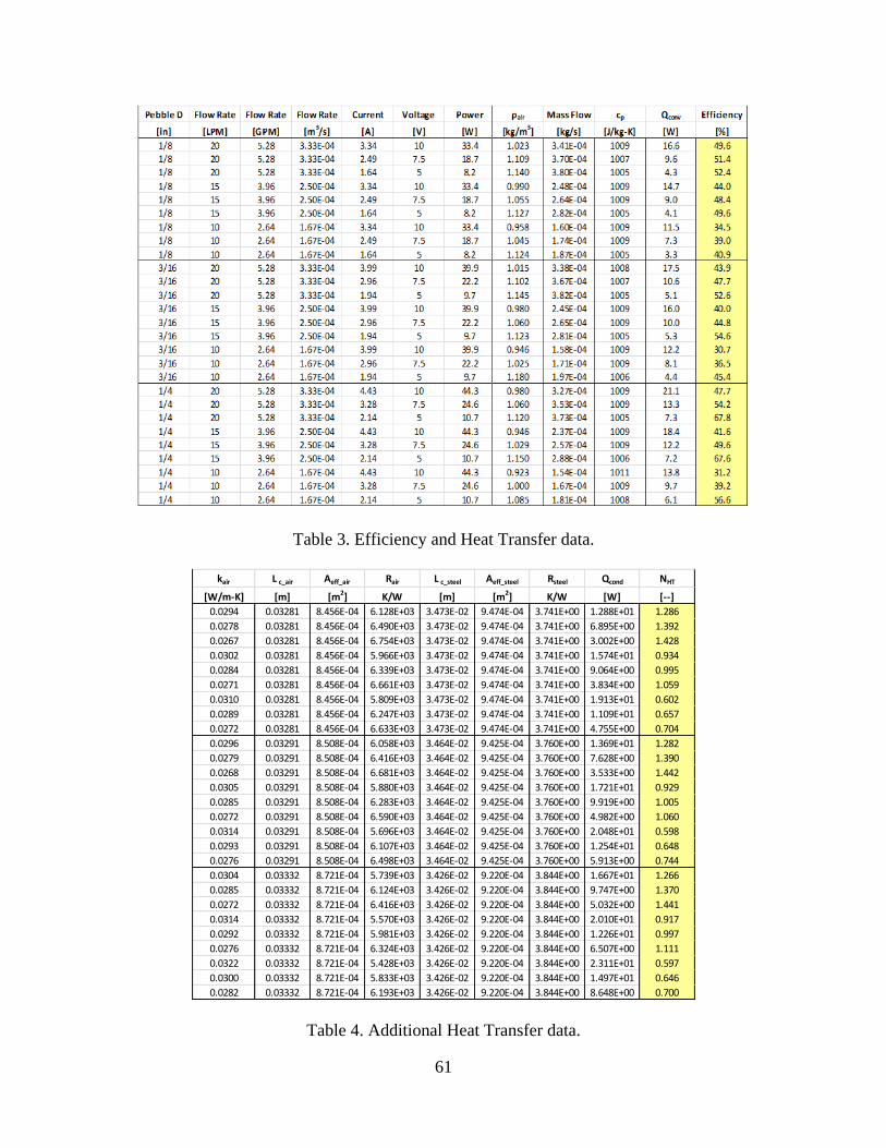
61

Table 3. Efficiency and Heat Transfer data.

Table 4. Additional Heat Transfer data.

kair L c_air Aeff_air Rair L c_steel Aeff_steel Rsteel Qcond NHT

[W/m-K] [m] [m2] K/W [m] [m2] K/W [W] [--]

0.0294 0.03281 8.456E-04 6.128E+03 3.473E-02 9.474E-04 3.741E+00 1.288E+01 1.286

0.0278 0.03281 8.456E-04 6.490E+03 3.473E-02 9.474E-04 3.741E+00 6.895E+00 1.392

0.0267 0.03281 8.456E-04 6.754E+03 3.473E-02 9.474E-04 3.741E+00 3.002E+00 1.428

0.0302 0.03281 8.456E-04 5.966E+03 3.473E-02 9.474E-04 3.741E+00 1.574E+01 0.934

0.0284 0.03281 8.456E-04 6.339E+03 3.473E-02 9.474E-04 3.741E+00 9.064E+00 0.995

0.0271 0.03281 8.456E-04 6.661E+03 3.473E-02 9.474E-04 3.741E+00 3.834E+00 1.059

0.0310 0.03281 8.456E-04 5.809E+03 3.473E-02 9.474E-04 3.741E+00 1.913E+01 0.602

0.0289 0.03281 8.456E-04 6.247E+03 3.473E-02 9.474E-04 3.741E+00 1.109E+01 0.657

0.0272 0.03281 8.456E-04 6.633E+03 3.473E-02 9.474E-04 3.741E+00 4.755E+00 0.704

0.0296 0.03291 8.508E-04 6.058E+03 3.464E-02 9.425E-04 3.760E+00 1.369E+01 1.282

0.0279 0.03291 8.508E-04 6.416E+03 3.464E-02 9.425E-04 3.760E+00 7.628E+00 1.390

0.0268 0.03291 8.508E-04 6.681E+03 3.464E-02 9.425E-04 3.760E+00 3.533E+00 1.442

0.0305 0.03291 8.508E-04 5.880E+03 3.464E-02 9.425E-04 3.760E+00 1.721E+01 0.929

0.0285 0.03291 8.508E-04 6.283E+03 3.464E-02 9.425E-04 3.760E+00 9.919E+00 1.005

0.0272 0.03291 8.508E-04 6.590E+03 3.464E-02 9.425E-04 3.760E+00 4.982E+00 1.060

0.0314 0.03291 8.508E-04 5.696E+03 3.464E-02 9.425E-04 3.760E+00 2.048E+01 0.598

0.0293 0.03291 8.508E-04 6.107E+03 3.464E-02 9.425E-04 3.760E+00 1.254E+01 0.648

0.0276 0.03291 8.508E-04 6.498E+03 3.464E-02 9.425E-04 3.760E+00 5.913E+00 0.744

0.0304 0.03332 8.721E-04 5.739E+03 3.426E-02 9.220E-04 3.844E+00 1.667E+01 1.266

0.0285 0.03332 8.721E-04 6.124E+03 3.426E-02 9.220E-04 3.844E+00 9.747E+00 1.370

0.0272 0.03332 8.721E-04 6.416E+03 3.426E-02 9.220E-04 3.844E+00 5.032E+00 1.441

0.0314 0.03332 8.721E-04 5.570E+03 3.426E-02 9.220E-04 3.844E+00 2.010E+01 0.917

0.0292 0.03332 8.721E-04 5.981E+03 3.426E-02 9.220E-04 3.844E+00 1.226E+01 0.997

0.0276 0.03332 8.721E-04 6.324E+03 3.426E-02 9.220E-04 3.844E+00 6.507E+00 1.111

0.0322 0.03332 8.721E-04 5.428E+03 3.426E-02 9.220E-04 3.844E+00 2.311E+01 0.597

0.0300 0.03332 8.721E-04 5.833E+03 3.426E-02 9.220E-04 3.844E+00 1.497E+01 0.646

0.0282 0.03332 8.721E-04 6.193E+03 3.426E-02 9.220E-04 3.844E+00 8.648E+00 0.700

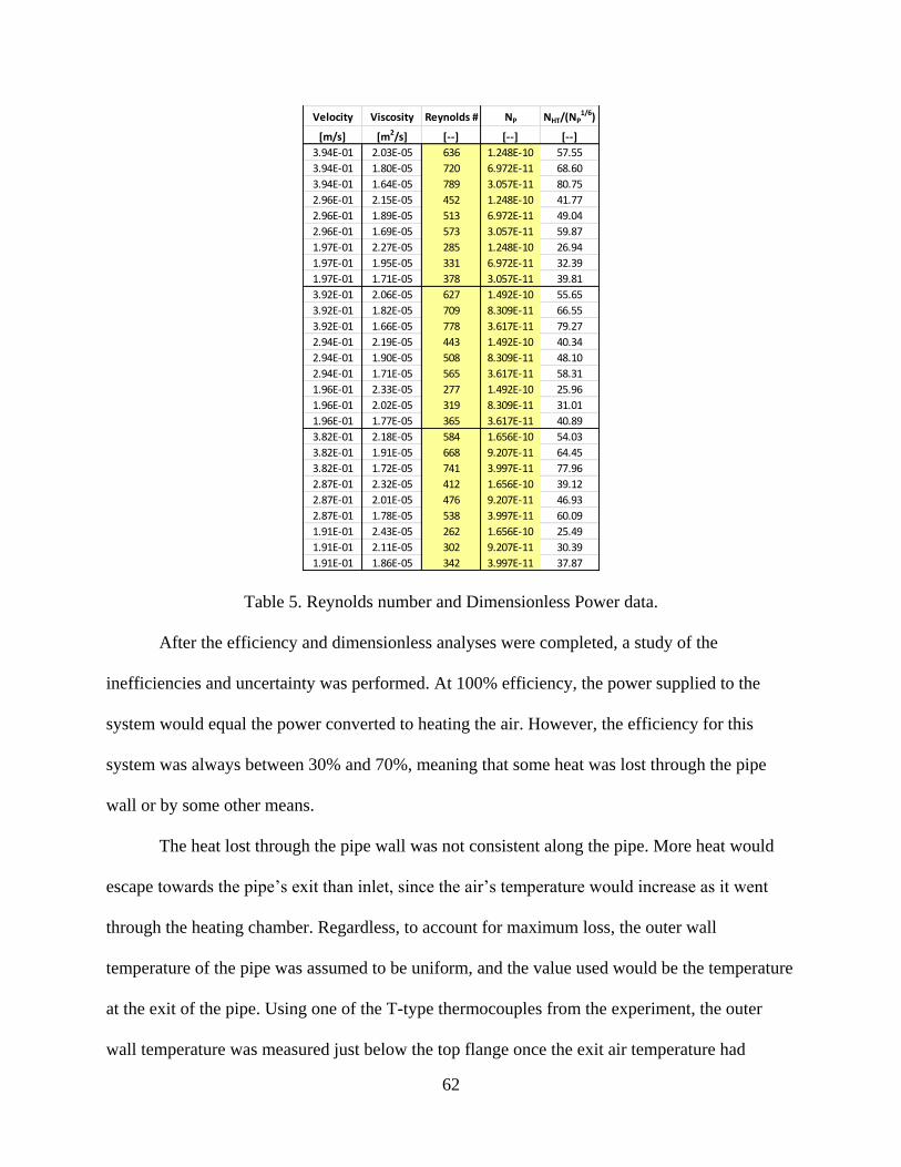
62

Table 5. Reynolds number and Dimensionless Power data.

After the efficiency and dimensionless analyses were completed, a study of the

inefficiencies and uncertainty was performed. At 100% efficiency, the power supplied to the

system would equal the power converted to heating the air. However, the efficiency for this

system was always between 30% and 70%, meaning that some heat was lost through the pipe

wall or by some other means.

The heat lost through the pipe wall was not consistent along the pipe. More heat would

escape towards the pipe’s exit than inlet, since the air’s temperature would increase as it went

through the heating chamber. Regardless, to account for maximum loss, the outer wall

temperature of the pipe was assumed to be uniform, and the value used would be the temperature

at the exit of the pipe. Using one of the T-type thermocouples from the experiment, the outer

wall temperature was measured just below the top flange once the exit air temperature had

Velocity Viscosity Reynolds # NP NHT/(NP1/6)

[m/s] [m2/s] [--] [--] [--]

3.94E-01 2.03E-05 636 1.248E-10 57.55

3.94E-01 1.80E-05 720 6.972E-11 68.60

3.94E-01 1.64E-05 789 3.057E-11 80.75

2.96E-01 2.15E-05 452 1.248E-10 41.77

2.96E-01 1.89E-05 513 6.972E-11 49.04

2.96E-01 1.69E-05 573 3.057E-11 59.87

1.97E-01 2.27E-05 285 1.248E-10 26.94

1.97E-01 1.95E-05 331 6.972E-11 32.39

1.97E-01 1.71E-05 378 3.057E-11 39.81

3.92E-01 2.06E-05 627 1.492E-10 55.65

3.92E-01 1.82E-05 709 8.309E-11 66.55

3.92E-01 1.66E-05 778 3.617E-11 79.27

2.94E-01 2.19E-05 443 1.492E-10 40.34

2.94E-01 1.90E-05 508 8.309E-11 48.10

2.94E-01 1.71E-05 565 3.617E-11 58.31

1.96E-01 2.33E-05 277 1.492E-10 25.96

1.96E-01 2.02E-05 319 8.309E-11 31.01

1.96E-01 1.77E-05 365 3.617E-11 40.89

3.82E-01 2.18E-05 584 1.656E-10 54.03

3.82E-01 1.91E-05 668 9.207E-11 64.45

3.82E-01 1.72E-05 741 3.997E-11 77.96

2.87E-01 2.32E-05 412 1.656E-10 39.12

2.87E-01 2.01E-05 476 9.207E-11 46.93

2.87E-01 1.78E-05 538 3.997E-11 60.09

1.91E-01 2.43E-05 262 1.656E-10 25.49

1.91E-01 2.11E-05 302 9.207E-11 30.39

1.91E-01 1.86E-05 342 3.997E-11 37.87

63

leveled off. With these temperature readings, the amount of heat lost through the wall could be

calculated using equation 23 [33]. The amount of power that did not go to heating the air or

escaping through the wall was called Qremaining and calculated with equation 24.

[ ] [

] [ ] [ ]

( [ ]

[ ])

[ ] [ ] [ ] [ ]

The amount of power remaining ranged from 9.63 watts to negative 3.44 watts as seen in

table 6, but in an ideal case it should be zero watts. There were three negative values greater than

1 watt for Qremaining, and each of them occurred at 5 volts. Either the quantity of heat escaping

through the pipe was too high or the heat to convection was too low. The opposite could be said

for the readings producing positive values greater than 1 watt. The inaccuracy in the amount of

Qremaining could be due to the fact that heat lost through the pipe was assumed to be uniform.

There could also be other sources of power loss in the induction heater system that were not

accounted for. The uncertainty of the power supplied, the heat to convection, and the heat lost

through the pipe were calculated and can be seen in table 6 along with the rest of the data from

this analysis. The calculated uncertainty was able to account for a few of the experiments, but

most fell outside of the range. Therefore, the uncertainty analysis does not completely account

for all error. A more in depth study into the losses of the induction heater system and the

temperature loss across the pipe would need to be conducted.

Eq. 23

Eq. 24

64

Table 6. Inefficiency data from all 27 experiments.

Pebble D Flow Rate

[in] [LPM]

1/8 20

1/8 20

1/8 20

1/8 15

1/8 15

1/8 15

1/8 10

1/8 10

1/8 10

3/16 20

3/16 20

3/16 20

3/16 15

3/16 15

3/16 15

3/16 10

3/16 10

3/16 10

1/4 20

1/4 20

1/4 20

1/4 15

1/4 15

1/4 15

1/4 10

1/4 10

1/4 10

Power

[W]

33.4

18.7

8.2

33.4

18.7

8.2

33.4

18.7

8.2

39.9

22.2

9.7

39.9

22.2

9.7

39.9

22.2

9.7

44.3

24.6

10.7

44.3

24.6

10.7

44.3

24.6

10.7

Qconv

[W]

16.6

9.6

4.3

14.7

9.0

4.1

11.5

7.3

3.3

17.5

10.6

5.1

16.0

10.0

5.3

12.2

8.1

4.4

21.1

13.3

7.3

18.4

12.2

7.2

13.8

9.7

6.1

Touter_wall Touter_wall Q loss_wall Qremaining U_Power U_Q_conv+loss Overlap

[F] [K] [W] [W] [W] [W] [--]

121.8 323.0 12.20 4.61 0.500 0.426 No

99.1 310.4 6.53 2.52 0.375 0.261 No

84.0 302.0 2.77 1.12 0.250 0.149 No

132.9 329.2 14.97 3.72 0.500 0.499 No

108.3 315.5 8.82 0.81 0.375 0.315 Yes

89.1 304.9 4.05 0.07 0.250 0.166 Yes

144.2 335.5 17.79 4.07 0.500 0.583 No

114.1 318.7 10.27 1.10 0.375 0.375 No

90.7 305.8 4.45 0.38 0.250 0.190 Yes

124.0 324.3 12.75 9.63 0.500 0.450 No

101.1 311.5 7.04 4.59 0.375 0.284 No

85.7 303.0 3.21 1.38 0.250 0.165 No

136.5 331.2 15.85 8.09 0.500 0.541 No

109.3 316.1 9.10 3.17 0.375 0.346 No

90.9 305.9 4.49 -0.09 0.250 0.201 Yes

150.1 338.8 19.25 8.44 0.500 0.618 No

120.7 322.4 11.93 2.18 0.375 0.416 No

96.2 308.8 5.83 -0.54 0.250 0.238 No

136.2 331.0 15.79 7.40 0.500 0.537 No

109.7 316.3 9.18 2.11 0.375 0.349 No

91.6 306.3 4.68 -1.24 0.250 0.209 No

149.1 338.2 18.99 6.88 0.500 0.621 No

119.1 321.6 11.53 0.87 0.375 0.418 No

97.1 309.3 6.04 -2.58 0.250 0.260 No

160.4 344.5 21.82 8.68 0.500 0.696 No

129.4 327.3 14.10 0.87 0.375 0.491 Yes

105.2 313.8 8.07 -3.44 0.250 0.316 No

65

CHAPTER 6

DISCUSSION

This study was able to research the capabilities and limitations of a magnetic induction

pebble-bed heater, design and construct a fully-functional scaled-down model, and determine a

pebble-bed heater’s behavior under different conditions. The following will be a discussion of

the research, experimental findings, potential improvements to the design, and future testing

possibilities.

The research in this study determined that if a pebble-bed heater was powered by

magnetic induction, it could only be a suitable nuclear reactor simulator for testing nuclear

thermal rocket engines if a metal was found that had a melting temperature well above 1,922 K

(3,000 °F) and was both magnetic and electrically conductive. However, if the pebble matrix is

heated by convection in the same manner as Glenn Research Center’s pebble-bed heater had

been in the mid 1960’s, it is possible to use it as a simulator, and high melting temperature

ceramics could be used in the pebble bed instead of steel. The downside to the convection

method is that it is limited to at most a 30 second test window before the pebble matrix has

cooled too much. This was the reason for looking into magnetic induction as a heat source, since

magnetic induction provides a continuous supply of heat, allowing tests to be run for as long as

necessary.

For the nuclear simulator case where a magnetic induction pebble-bed heater will actually

be used as a nuclear reactor simulator, several important characteristics should be considered

when choosing the steel type and grade that will make up the pebble matrix and chamber. First,

the steel must be hydrogen-embrittlement-free, since the propellant that will be used for the

nuclear rocket engines is hydrogen. Hydrogen embrittlement is a destructive process that makes

66

high strength steels brittle and eventually fracture after exposure to high temperature hydrogen

[4]. At high temperatures, hydrogen atoms can actually seep into certain metals. If several

hydrogen atoms gather together in a small pocket inside the metal and form molecules, then the

molecules can begin to create internal pressure and eventually cause the metal to crack open [4].

Embrittlement is most commonly found in high strength and low alloy steels, so these should be

avoided. It would be a disaster if the chamber cracked, and fractured steel balls could skew

results.

Secondly, the metal for the spheres must be magnetic and have a very high melting

temperature, as it will obviously be operating at several thousand degrees Kelvin. Melting

temperatures for stainless steels range from 1,672 K to 1,803 K (2,550 °F to 2,785 °F), and

carbon steels range from 1,683 K to 1,811 K (2,570 °F to 2,800 °F) [10,19]. Even though certain

high carbon steels can sustain a slightly greater temperature than the stainless steels, they are not

as corrosive resistant or embrittlement-free as some of the stainless steels. It is therefore

recommended to choose stainless steel over carbon steel in the nuclear simulator tests. The two

stainless steel grades with the highest melting temperature are grades 409 and 410 [10]. Grade

409 is a ferritic stainless steel and subsequently prone to hydrogen embrittlement. Grade 409 is

therefore not an option for nuclear testing [8]. However, grade 410 is a martensic stainless steel,

which makes it hydrogen-embrittlement-free and magnetic [8]. In conclusion, grade 410 stainless

steel is the best candidate for the steel pebbles inside the pebble matrix for the nuclear reactor

simulator. If a hydrogen-embrittlement-free steel is later manufactured with a higher melting

temperature, then it would clearly be a more suitable option.

In addition to the melting temperature, another setback to the magnetic induction method

is the Curie temperature of steel. The Curie temperature is the point at which a material is no

67

longer magnetic and for most steels this is usually around 1,033 K (1,400 °F). To be a simulator,

the heater would need to heat hydrogen up to 1,922 K (3,000 °F). Beyond the Curie temperature,

heating is still possible with induction heating but without the hysteresis loss portion of the heat

generation. The process would be much slower past this point and require additional power,

since only the skin effect would be heating the steel.

A magnetic induction pebble-bed heater still has other beneficial uses besides a nuclear

reactor simulator, especially at lower temperature levels. Due to its high efficiency, no moving

parts, and non-invasive, flameless method of heating gases and fluids, there are many possible

applications for the heater. The device was found to have been used on at least two other

experiments. One was to test the cooling capabilities of salt by putting a specialized salt in a tube

full of graphite spheres and heating the graphite with an induction heater. Another experiment

was to test the cooling abilities of a metal tube packed with little balls inside that has air flowing

through it compared to a solid metal pipe with air flowing over it. It could also be used in a home

as a local hot water heater for a sink/shower or any instance where a gas, liquid, or even a metal

object inside a tube needed to be heated without a flame or any invasive tactics.

The design of the experiment allowed all 27 tests to be run and data to be recorded. The

better aspects of the pebble-bed heater design from this experiment include the two middle

copper spacers and the bronze wool. The copper spacers allowed the temperature and pressure

measuring instruments access to the air flow directly before and after the heating process without

allowing any air to leak out. The bronze wool successfully normalized the flow of the air, so that

it had a uniform distribution when it met the two sets of instruments and when it entered the

pebble matrix.

68

The pebble-bed heater design had several flaws. The main issues being insulation and

weight. In order to hopefully solve the insulation issue in the future, the center section of the

pebble-bed heater should be made out of a high melting temperature ceramic. Since aluminum,

brass, and copper are all conductive, none of them are suitable candidates. Conductive metals

would not only be affected by the skin effect but would also risk shorting out the system if any

contact is made with the work coil of the induction heater. While 3D printed ABS plastic was a

great substitute for this low temperature test environment, it would not be feasible for most

applications given its low “melting” temperature. Therefore, a ceramic with a high melting

temperature should be used as the material for the pebble chamber and be molded or 3D printed

into the appropriate flange-pipe-flange shape for the job at hand. The chamber could also be

wrapped or coated in additional insulation to reduce heat lost through conduction in the pipe wall

and improve the overall efficiency.

There was another insulation issue with the upstream thermocouple and the differential

pressure transducer (DPT). The induced current from the work coil would interfere with the DPT

and first thermocouple’s readings, so all pressure and intake temperature readings were recorded

once the maximum temperature was reached and just after the induction heater was turned off.

The exit temperature and volumetric flow rate would be the same but without the electrical

interference. To resolve this issue, there should be a rubber or non-conductive thin layer between

the instrument spacers and the center section. In addition, the metal mesh circles could be

attached to the rubber washer instead of cardboard. To insulate the DPT, it should be placed on

top of a piece of wood, cardboard, plastic, or other non-conductive material. These adjustments

were not performed in this set of experiments but will hopefully reduce the amount of

interference from induced currents in the future.

69

The second major issue with the design was the weight of the pebble-bed heater. Copper

was chosen as the material for most of the heater, since it was not magnetic and easy to machine;

however, copper is both heavy and expensive. Copper was the main material used in this

experiment, so the system weighed close to 111 N (25 lb). In hind sight, aluminum would be the

best option for the disk spacers in the middle and at either end. Copper is 73% heavier than

aluminum, so switching to aluminum would eliminate a lot of the weight [57]. The thickness of

the end spacers could also be cut in half, and it would still be more than enough for the NPT

fittings on either end to screw in. In order to remove all copper, the two smaller flange-pipe-

flange sections could be made out of aluminum or the same high melting temperature ceramic as

the center pipe section. Aluminum would work for these sections because there is no chance of

touching the work coil.

The induction heater schematic chosen was fitting for this application. The heater was

easy enough for someone with minimal electrical experience to learn how it worked and put all

the pieces together. There were not many components, and the parts were not difficult to find or

expensive. Lastly, this circuit was capable of heating metal to almost 533 K (500 °F), which was

more than enough for the experiment.

Several improvements that could be made to the induction heater would be the work coil

and the addition of a breadboard. The one-piece, 0.847 cm (1/3”), copper pipe originally used in

the experiment produced higher temperatures than the 12 gauge insulated wire that was later put

in its place. The pipe could also handle higher currents and even be water cooled if the pipe were

to get too hot. If the pipe, flanges, and bolts are either non-conductive or insulated from the

solenoid, then the copper pipe should be used for the solenoid.

70

Since the breadboards in the lab were only able to support up to one amp of current, a

floating circuit had to be made. However, it is recommended that a breadboard be purchased that

could handle 5 amps or maybe even more than 5 amps and used for the induction heater circuit.

The resistors, diodes, capacitors, and transistors could then easily be securely connected to the

breadboard, power supply, and one another. One of the frequent issues during the testing process

was with the wires attached to the transistors. The wires would occasionally be bumped, and the

solder would come loose, then the transistors would short circuit instantly and need to be

replaced. If the transistors could be plugged straight into a breadboard, then the problem would

not be as likely to happen. This would allow for less maintenance and fewer transistors would

need to be ordered.

The behavior of the heater was tested over 27 experiments at different conditions. This

study shows how the exit temperature is affected by the flow rate, pebble size, and power level.

It was found that the amount of temperature change would increase with increasing pebble size,

decreasing flow rate, and increasing power. As the flow rate decreased, it would take longer for

the test to reach the maximum temperature. This should be taken into account if time is a factor.

Changing the amount of power supplied to the system had the quickest effect on the temperature.

Therefore, increasing the power is the best way to increase the exit temperature. The overall

efficiency would decrease as the power increased and as the flow rate decreased, so a higher exit

temperature would mean more wasted power.

After a series of calculations, the Dimensionless Heat Transfer, Dimensionless Power,

and Reynolds number were calculated for each of the 27 cases. The results were put into a chart,

so that the data can be used to predict the capabilities of a future pebble-bed heater or verify the

results of an existing pebble-bed heater. The same characteristic length formula should be used

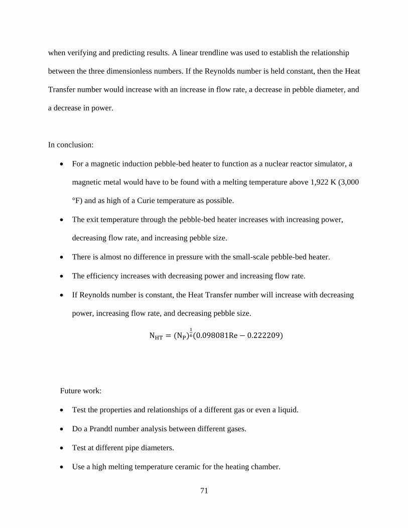
71

when verifying and predicting results. A linear trendline was used to establish the relationship

between the three dimensionless numbers. If the Reynolds number is held constant, then the Heat

Transfer number would increase with an increase in flow rate, a decrease in pebble diameter, and

a decrease in power.

In conclusion:

For a magnetic induction pebble-bed heater to function as a nuclear reactor simulator, a

magnetic metal would have to be found with a melting temperature above 1,922 K (3,000

°F) and as high of a Curie temperature as possible.

The exit temperature through the pebble-bed heater increases with increasing power,

decreasing flow rate, and increasing pebble size.

There is almost no difference in pressure with the small-scale pebble-bed heater.

The efficiency increases with decreasing power and increasing flow rate.

If Reynolds number is constant, the Heat Transfer number will increase with decreasing

power, increasing flow rate, and decreasing pebble size.

Future work:

Test the properties and relationships of a different gas or even a liquid.

Do a Prandtl number analysis between different gases.

Test at different pipe diameters.

Use a high melting temperature ceramic for the heating chamber.

72

Use a small, copper pipe instead of a thick wire for the work coil.

Put the circuit in a 5 amp or more breadboard

Electrically insulate the middle instrumentation disks from the heating chamber

Use more aluminum and less copper for the parts of the experiment (except the work

coil)

73

REFERENCES

[1] Acero, J., et al. "The domestic induction heating appliance: An overview of recent research"

Applied Power Electronics Conference and Exposition, 2008. APEC 2008. Twenty-Third Annual

IEEE (Feb 2008): 651-657. Presented.

[2] Anderson, W. & Heister, S. (2005). Purdue Propulsion: Rocket Propulsion Short Course

Notes. Purdue University School of Aeronautics and Astronautics. West Lafayette, IN. Print.

[3] ASM International. "Theory of Heating by Induction." Practical Induction Heat Treating.

2001. Print.

[4] Barnoush, Afrooz. Hydrogen Embrittlement. Tech. 2011. Print. <http://www.uni-

saarland.de/fak8/wwm/research/phd_barnoush/hydrogen.pdf>.

[5] Braun, Bobby. "Open Letter to College Students." NASA. Letter. 9 Aug. 2010.

<http://www.nasa.gov/offices/oct/home/college_letter_detail.html>.

[6] Burnett, Richie. "High Frequency Induction Heating." Web. 3 Mar. 2013.

<http://www.richieburnett.co.uk/indheat.html>.

[7] Corliss, William R., and Francis C. Schwenk. "NERVA Flow Diagram." Nuclear Propulsion

for Space. NASA, 1971. Web. 21 Jan. 2014.

[8] CSI Equipment and Services. Stainless Steel Selection Guide - Central States Industrial,

Central States Industrial Equipment and Services Inc., Springfield, MO., 2001. Print.

<http://www.csidesigns.com/PDFs/SSSguide.pdf>.

[9] Davenne, Tristan, Otto Caretta, and Peter Loveridge. A Static Packed Bed Target.

Presentation. 2011.

[10] Davis, Joseph R. ASM Specialty Handbook Stainless Steels. ASM International, 1995. Print.

[11] Digikey. "1N4007-E3/54GICT-ND: Schottky Rectifier Diode, 1 A, 1 kV." Web. 20 Apr.

2013. <http://www.digikey.com/product-detail/en/1N4007-E3%2F54/1N4007-E3%2F54GICT-

ND/868990>.

[12] Digikey. "497-7520-5-ND: MOSFET Transistor, N-Channel, 100 V, 35 A." Web. 22 Apr.

2013. <http://www.digikey.com/product-search/en?lang=en&site=us&KeyWords=497-7520-5-

nd&x=0&y=0>.

[13] Digikey. "BC1910-ND: 330 NF Film Capacitor, 1 KV, Radial." Web. 18 Apr. 2013.

<http://www.digikey.com/product-search/en?vendor=0&keywords=bc1910-nd>.

74

[14] Digikey. "HS276-ND: TO-220 Heat Sink." Web. 22 Apr. 2013.

<http://www.digikey.com/product-search/en?WT.z_header=search_go&lang=en&site=

us&keywords=hs276-nd&formaction=on&x=0&y=0>.

[15] Engineer’s Handbook. "Engineering Materials - Non Ferrous Metals." Web. 29 Jan. 2014.

<http://www.engineershandbook.com/Materials/nonferrous.htm>.

[16] Engineering Toolbox. "Air - Absolute and Kinematic Viscosity." Web. 23 Feb. 2014.

<http://www.engineeringtoolbox.com/air-absolute-kinematic-viscosity-d_601.html>.

[17] Engineering Toolbox. "Air - Density and Specific Weight." Web. 23 Feb. 2014.

<http://www.engineeringtoolbox.com/air-density-specific-weight-d_600.html>.

[18] Engineering Toolbox. "Air Properties." Web. 23 Feb. 2014.

<http://www.engineeringtoolbox.com/air-properties-d_156.html>.

[19] Engineering Toolbox. "Metals - Melting Temperature." Web. 28 Jan. 2014.

<http://www.engineeringtoolbox.com/melting-temperature-metals-d_860.html>.

[20] Engineering Toolbox. "Thermal Conductivity of Some Common Materials and Gases."

Web. 23 Feb. 2014. <http://www.engineeringtoolbox.com/thermal-conductivity-d_429.html>.

[21] Esselman, W. H. "The NERVA Nuclear Rocket Reactor Program." Westinghouse Engineer

25.3 (1965): 65-75. Print. <http://pbhistoryb1b3.grc.nasa.gov/assets/history/B%20NERVA/

NERVA%20Nuclear%20Rocket%20Program%20(1965).PDF>.

[22] Fairchild Semiconductor. Induction Heating System Topology Review. Tech. no. AN-9012.:

Fairchild Semiconductor, 2000. Print.

[23] Fortuner 4x4. "Wire Gauge Calculation Chart - Maximum Current Draw." Fortuner 4x4

Fans. Web. 15 Apr. 2013. <http://www.fortuner4x4fans.co.za/forum/index.php?page=

Attachment&attachmentID=299&h=be8b440dbf9c008d2615285ebd0599ef25ddea6d>.

[24] Future Electronics. "Schottky Rectifiers." Web. 20 Apr. 2013.

<http://www.futureelectronics.com/en/diodes/schottky-rectifiers.aspx>.

[25] General Applied Science Laboratory (GASL) (1995). Systems Operation Manual for Pebble

Bed Hydrogen Heater installed at NASA John C. Stennis Space Center. Ronkonkoma, NY. Print.

[26] GH Induction Atmospheres. "Innovative Induction Heating." Web. 2 July 2013.

<http://www.gh-ia.com/induction_heating.html>.

[27] Grainger. "1WLH5: Flange, Cast Copper, C x Flange, 1 in." Web. 2 Apr. 2013.

<http://www.grainger.com/product/NIBCO-Flange-1WLH5?s_pp=false>.

75

[28] Hobby Lobby. "491621: Large Activ-Wire Mesh, Aluminum." Web. 9 Apr. 2013.

<http://shop.hobbylobby.com/products/large-activ-wire-mesh-491621/>.

[29] Home Depot. "123100: Homax Fine Bronze Wool Pads (3 Pack)." Web. 6 Apr. 2013.

<http://www.homedepot.com/p/Homax-Fine-Bronze-Wool-Pads-3-Pack-123100/100185012>.

[30] Houts, M. G., et al. "Nuclear Thermal Propulsion for Advanced Space Exploration." NASA

(2011). NTRS. Print. <http://ntrs.nasa.gov/archive/nasa/casi.ntrs.nasa.gov/

20120014974_2012014786.pdf>.

[31] Iatcheva, Ilona, Georgi Gigov, Georgi Kunov, and Rumena Stancheva. "Analysis of

Induction Heating System for High Frequency Welding." Electrical Engineering 25.3 (2012):

183-91. Print.

[32] Jackson, John D. Classical Electrodynamics. 3rd ed.: Hamilton Printing, 1999. Print.

[33] Kreith, Frank, and Mark S. Bohn. Principles of Heat Transfer. 6th ed. Ontario: Chris

Carson, 2001. Print.

[34] Lancashire, R. B., E. A. Lezberg, and J. F. Morris. "Heat-Transfer Coefficients for Full-

Scale Pebble-Bed Heater." Industrial and Engineering Chemistry 52.5 (1960): 433-34. Print.

[35] Lupi, S. "The Calculation of Planar Circular Coils for the Induction Heating of Bimetallic

Plates." Archiv Fur Elektrotechnik 60.6 (1978): 313-318. Springer. Web. 27 Jan. 2014.

[36] Materkowski, Dave. "How NASA's NERVA Rocket Engine Works." ART 101. Web. 20

Jan. 2014. <http://www.personal.psu.edu/djm5200/NERVA.html>.

[37] McCurrie, R. A. Ferromagnetic Materials: Structure and Properties. San Diego: Academic,

1994. Print.

[38] Meng, L.; Cheng, K.; Chan, K. “Heating Performance Improvement and Field Study of the

Induction Cooker.” Power Electronics Systems and Applications, 2009. PESA 2009. 3rd

International Conference (May 2009): 1-5. Presented.

[39] Mouser. "70-IHV-15-500: 500 uH Inductor, Radial." Web. 17 Apr. 2013.

<http://www.mouser.com/ProductDetail/Vishay/IHV15BZ500/?qs=%2fha2pyFadugmQTbFDrn

uErOv8Ng0ztPFw8%2fYvy%2fHTBqda9UGY3u0dA%3d%3d>.

[40] MSC Industrial Supply. "00073239: Carbon Steel Ball Bearing, 1/8 Inch." Web. 7 Apr.

2013. <http://www.mscdirect.com/product/00073239?rItem=00073239>.

[41] Mühlbauer, Alfred. "Background of Induction Heating." History of Induction Heating and

Melting: Vulkan-Verlag GmbH, 2008. Print.

76

[42] NASA. "Aerial A,B." Stennis Image Retrieval System. 30 Apr. 2004. Web. 20 Jan. 2014.

<http://www.ssc.nasa.gov/sirs/scripts/getxmlfile.pl?id=SSC-2004-02813>.

[43] NASA. Glenn Research Center. The NASA Glenn Research Center's Hypersonic Tunnel

Facility. By Mark R. Woike and Brian P. Willis. 2001. Print.

[44] NASA. Lewis Research Center. An Historical Perspective of the NERVA Rocket Engine

Technology Program. By W. H. Robbins and H. B. Finger. 1991. Print.

[45] NASA. "NERVA Engine Testing." History B-1 and B-3 Test Stands. NASA. Web. 27 Jan.

2014. <http://pbhistoryb1b3.grc.nasa.gov/NERVA.aspx>.

[46] NASA. "Static Test Firing of Saturn V S-1C Stage." Great Images in NASA. 1 Jan. 1967.

Web. 20 Jan. 2014. <http://dayton.hq.nasa.gov/IMAGES/LARGE/GPN-2000-000041.jpg>.

[47] NDT Resource Center. "The Hysteresis Loop and Magnetic Properties." Web. 7 July 2013.

<http://www.ndt-

ed.org/EducationResources/CommunityCollege/MagParticle/Physics/HysteresisLoop.htm>.

[48] Norton, O. & Palmer, R. (2005). Technology to Support the Design of a Nuclear Propulsion

and Power Test Facility. DIAL at Mississippi State University. Stennis Space Center, MS. Print.

[49] Omega. "PX157-005DI Manual: Differential Pressure Transducer." Web. 11 Apr. 2013.

<http://www.omega.com/Manuals/manualpdf/M1997.pdf>.

[50] Omega. "Thermocouples." Web. 10 Apr. 2013.

<http://www.omega.com/prodinfo/thermocouples.html>.

[51] Omega. "TMQSS-062G-6: T-Type, 6 Inch, Grounded, 1/16 Inch." Web. 10 Apr. 2013.

<http://www.omega.com/pptst/JMQSS.html>.

[52] Omega. "Type T Revised Thermocouple Reference Tables." Web. 10 Apr. 2013.

<http://www.omega.com/temperature/Z/pdf/z223.pdf>.

[53] Osborn, H. B., Jr., et al. Induction Heating. Cleveland: 1946. Print.

[54] Osofsky, Irving B. Pebble-Bed Heater and Shock Tube Assembly. Sparta, Inc., assignee.

Patent US 5197323 A. 13 July 1990. Print.

[55] Palaszewski, B. (2004). Nuclear and Future Flight Propulsion: Vehicle Design Case

Studies. Glenn Research Center. Cleveland, OH. Print.

[56] Plumbing Supply. "Rigid Copper Pipe." Web. 1 Apr. 2013.

<http://www.plumbingsupply.com/copperpipe.html>.

77

[57] Pryor, Larry, Rick Schlobohm, and Bill Brownell. "A Comparison of Aluminum vs. Copper

as Used in Electrical Equipment." GE Consumer and Industrial. Web. 11 Feb. 2014.

<http://apps.geindustrial.com/publibrary/checkout/Alum-Copper?TNR=White%20Papers%

7CAlum-Copper%7Cgeneric>.

[58] Rauch, R.; Coote, D.; Junnell, J.; & Ryan, H. (2011). The Nuclear Propulsion and Power

Non-Nuclear Test Facility CIF Request. Stennis Space Center. Print.

[59] Rauch, R. & Raines, N. Technology to Support the Design of a Nuclear Propulsion and

Power Non-nuclear Test Facility CDDF Final Report. (2005). Stennis Space Center. Print.

[60] Rhoades, Nathan. "A Fundamental Overview of Heating by Induction." (2006). Web. 26

Jan. 2014. Print.

[61] RMCybernetics. “A DIY Induction Heater.” Research Media and Cybernetics. Web. 20

Apr. 2013. <http://www.rmcybernetics.com/projects/DIY_Devices/diy-induction-heater.htm>.

[62] RMCybernetics. "RES0W6: 240 Ohm Resistor, 0.6 Watt." Web. 19 Apr. 2013.

<http://www.rmcybernetics.com/shop/electronic-components/resistors/resistors-0.6W>.

[63] Russo, E.; Rieder, P.; Castrogiovanni, A.; St. Cyr, W. (1996). Thermal Analysis of NASA’s

John C. Stennis Space Center’s Pebble-Bed Heater. Stennis Space Center. Stennis Space Center,

MS. Print.

[64] Serway, Raymond A., and John W. Jewett, Jr. Physics for Scientists and Engineers with

Modern Physics. 7th ed. Belmont, CA: Thomson/Brooks/Cole, 2008. Print.

[65] Simons, E.N. A Dictionary of Alloys. Cornell University. 1970. Print.

[66] ST Microelectronics. STP30NF10 MOSFET Manual. Web. 25 Apr. 2013.

<http://www.st.com/web/en/resource/technical/document/datasheet/CD00002440.pdf>.

[67] Stansel, N. R. Induction Heating. 1st ed. New York City: McGraw-Hill Book, 1949. Print.

[68] Stratasys. "ABS." Web. 31 Jan. 2014. <http://www.nrri.umn.edu/NLTC/ABS07.pdf>.

[69] Swagelok. "B-1RS4: Brass, Needle Valve, 1/4 In, T-shape." Web. 4 Apr. 2013.

<http://www.swagelok.com/search/find_products_home.aspx?part=B-1RS4&item=>.

[70] Swagelok. "B-42S4: Brass, Ball Valve, 1/4 In, T-shape." Web. 31 Jan. 2014.

<http://www.swagelok.com/search/find_products_home.aspx?part=B-42S4&item=5c7e79e8-

62ca-4c16-8b6e-0ba1530cbfd7>.

[71] Swagelok. "B-100-1-2BT: Brass, Straight Tube Fitting, 1/16 In, Male NPT, Bored-

Through." Web. 11 Apr. 2013. <http://www.swagelok.com/search/find_products_home.aspx?

part=B-100-1-2BT&item=>.

78

[72] Swagelok. "B-400-1-4: Brass, Straight Tube Fitting, 1/4 In, Male NPT." Web. 4 Apr. 2013.

<http://www.swagelok.com/search/find_products_home.aspx?part=B-400-1-4&item=20b6dcb5-

5a04-42f1-9df7-a5d3fd3672c3>.

[73] Swagelok. "B-400-1-4BT: Brass, Straight Tube Fitting, 1/4 In, Male NPT, Bored-Through."

Web. 11 Apr. 2013. <http://www.swagelok.com/search/find_products_home.aspx?part=B-400-

1-4BT&item=>.

[74] Tech Power Up. "What Is a MOSFET, What Does It Look Like, and How Does It Work?"

24 May 2004. Web. 6 Feb. 2014.

<http://www.techpowerup.com/articles/overclocking/voltmods/21>.

[75] Tudbury, C. A. "Electromagnetics in Induction Heating." IEEE Transactions on Magnetics

10.3 (1974): 694-97. IEEE. Web. 25 Jan. 2014. Print.

[76] Weber, Louis J. Pebble Heater System and Method of Operation. Phillips Petroleum

Company, assignee. Patent US 2,530,274. 9 Dec. 1946. Print.

[77] Wtshymanski. "Induction Cooktop Rolling Boil." CommonsHelper, 6 Jan. 2011. Web. 27

Jan. 2014.

[78] Yoder, Graydon L., et al. An Experiment to Study Pebble Bed Liquid-Fluoride-Salt Heat

Transfer. Proc. of ICAPP, Nice, France. 2013. Print.

[79] Youhua, Wang, Wang Junhua, Li Jiangui, and Li Haohua. "Analysis of Induction Heating

Eddy Current Distribution Based on 3D FEM." Computational Technologies in Electrical and

Electronics Engineering (2008): 238-41. IEEE Xplore. Web. 20 Mar. 2013.

[80] 80/20 Inc. "80/20 Home Page." Web. 3 Feb. 2014. <http://www.8020.net/Default.asp>.

79

APPENDIX

1) Step-by-step assembly process of the pebble-bed heater:

80

81

2) Extra Uncertainty Data:

U_Current 0.05 A

U_Voltage 0.005 V

U_vol_flow 8.3333E-06 m3/s

U_Density 0 kg/s

U_Temp 0.1111111 K

U_c_p 0 J/kg-K

U_k_plastic 0 W/m-K

U_L_wall 0 m

U_r_out 0 m

U_r_in 0 m

U_number 0 --

U_r_ball 0 m

U_freq 10 Hz

r_in 0.0127 m (0.5")

r_out 0.01905 m (0.75")

L_wall 0.1397 m (5.5")

k_plastic 0.25 W/m-K

U_massflow U_ΔT U_Q_conv U_ΔT_wall U_Q_loss U_Q_cond U_N_HT U_Np U_Nu/Np

[kg/s] [K] [W] [K] [W] [W] [--] [--] [--]

8.525E-06 0.157 0.418 0.1571 0.085 0.418 0.053 1.88E-12 2.368

9.242E-06 0.157 0.247 0.1571 0.085 0.247 0.061 1.41E-12 3.034

9.500E-06 0.157 0.123 0.1571 0.085 0.123 0.071 9.36E-13 4.054

8.250E-06 0.157 0.491 0.1571 0.085 0.491 0.043 1.88E-12 1.914

8.792E-06 0.157 0.304 0.1571 0.085 0.304 0.047 1.41E-12 2.334

9.392E-06 0.157 0.142 0.1571 0.085 0.142 0.054 9.36E-13 3.075

7.983E-06 0.157 0.576 0.1571 0.085 0.576 0.035 1.88E-12 1.576

8.708E-06 0.157 0.365 0.1571 0.085 0.365 0.039 1.41E-12 1.946

9.367E-06 0.157 0.170 0.1571 0.085 0.170 0.044 9.36E-13 2.480

8.458E-06 0.157 0.442 0.1571 0.085 0.442 0.052 1.88E-12 2.281

9.183E-06 0.157 0.271 0.1571 0.085 0.271 0.061 1.41E-12 2.923

9.542E-06 0.157 0.141 0.1571 0.085 0.141 0.070 9.36E-13 3.862

8.167E-06 0.157 0.534 0.1571 0.085 0.534 0.042 1.88E-12 1.842

8.833E-06 0.157 0.335 0.1571 0.085 0.335 0.048 1.41E-12 2.295

9.358E-06 0.157 0.182 0.1571 0.085 0.182 0.053 9.36E-13 2.932

7.884E-06 0.157 0.613 0.1571 0.085 0.613 0.035 1.88E-12 1.515

8.542E-06 0.157 0.407 0.1571 0.085 0.407 0.039 1.41E-12 1.854

9.833E-06 0.157 0.222 0.1571 0.085 0.222 0.047 9.36E-13 2.579

8.167E-06 0.157 0.530 0.1571 0.085 0.530 0.051 1.88E-12 2.192

8.833E-06 0.157 0.338 0.1571 0.085 0.338 0.059 1.41E-12 2.776

9.333E-06 0.157 0.191 0.1571 0.085 0.191 0.066 9.37E-13 3.608

7.884E-06 0.157 0.615 0.1571 0.085 0.615 0.042 1.88E-12 1.774

8.575E-06 0.157 0.410 0.1571 0.085 0.410 0.047 1.41E-12 2.223

9.583E-06 0.157 0.245 0.1571 0.085 0.245 0.056 9.37E-13 3.056

7.689E-06 0.157 0.691 0.1571 0.085 0.691 0.035 1.88E-12 1.486

8.330E-06 0.157 0.484 0.1571 0.085 0.484 0.038 1.41E-12 1.813

9.042E-06 0.157 0.304 0.1571 0.085 0.304 0.043 9.37E-13 2.327