Experimental and theoretical studies of the aureole about a point source that is due to atmospheric...

Experimental and theoretical studies of theaureole about a point source that is due toatmospheric scattering in the middle ultraviolet

Claire Lavigne, Antoine Roblin, Patrick Chervet, and Patrick Chazette

In the atmosphere, pointlike sources are surrounded by aureoles because of molecular and aerosolscattering. In various meteorological conditions, this variance field can be a nonnegligible part of thesignal detected by a large-field-of-view sensor. A model based on a Monte Carlo technique has beendeveloped to simulate the propagation of radiation coming from a UV point source. The model wasvalidated with an experimental comparison by a photon-counting technique, and good agreement be-tween experimental and theoretical results was found. © 2005 Optical Society of America

OCIS codes: 010.1310, 030.5260, 030.5620, 120.5820, 260.7190, 290.4210.

1. Introduction

Scattering of light by molecules and aerosols in theatmosphere gives rise to a radiance field about apointlike source. The contribution of this radiationfield, or aureole, to the irradiance of a wide-field-of-view (FOV) sensor depends on many parameters,such as single-scattering albedo, optical thickness,and the source intensity’s angular properties. Insome situations the aureole’s contribution may be anonnegligible part of the detected signal, especiallyfor a large-FOV sensor. Such is usually the case in theEarth’s lower atmosphere when a sensor with a spec-tral band limited to the middle UV (typically240–290 nm) looks to a point source located a fewkilometers away. In this spectral domain, also calledthe solar-blind band, the Sun’s irradiance is com-pletely absorbed by stratospheric and troposphericozone layers, and no natural light reaches the Earth’slower atmosphere. So the source intensity can be re-corded with a low background, nearly entirely as aresult of the detector’s dark current. Because some

UV detectors do have low dark current and high sen-sitivity, the aureole may be observed, in some cases,with high contrast. The aureole’s influence is in-creased further when the original light source is par-tially shaded or when the intensity shows a minimumin the detector direction.

There has been increasing interest in exploitingthe unique features of the UV solar-blind band forvarious outdoor applications such a detection of firesand missiles plumes and in non-line-of-sight opticalcommunications.1,2 This interest will continue in thefuture, as new solid-state UV detectors based onnitride-III AlGaN semiconductors become available.3To evaluate the performance and limits of these ap-plications, one needs to understand accurately thephysical process that comprises source emission, at-mospheric propagation, and signal detection. A quan-titative description of the atmospheric propagation isalso necessary to correct the source intensity’s mea-surements from scattering effects. Various ap-proaches have already been developed to computeaureoles’ properties. Generally, Monte Carlo methodsare used as soon as the effects of the Earth’s ground,nonhomogeneous atmosphere, and nonisotropicsource emission must be taken into account in thecomputations. These models have permitted the un-derstanding of effects of various parameters, such asthe optical depth that corresponds to the distancebetween the source and the sensor, the single-scattering albedo, the source intensity’s anisotropy,and the line-of-sight direction, on the aureole’s prop-erties. However, few experimental data to validatethese computations have been reported. Despite the

C. Lavigne ([email protected]), A. Roblin, and P. Chervet arewith the Département d’Optique Théorique et Appliquée, OfficeNational des Etudes et Recherches Aérospatiales, Chemin de laHunière, 91761 Palaiseau Cedex, France. P. Chazette is with theLaboratoire des Sciences du Climat et de l’Environnement, Labo-ratoire Mixte Commissariat a l’Energie–Centre National de la Re-cherche Scientifique, F-91191 Gif-Sur-Yvette, France.

Received 23 January 2004; revised manuscript received 22 Oc-tober 2004; accepted 26 October 2004.

0003-6935/05/071250-13$15.00/0© 2005 Optical Society of America

1250 APPLIED OPTICS � Vol. 44, No. 7 � 1 March 2005

fact that Monte Carlo results can be obtained withprescribed accuracy, there are two main reasons thatthey could become erroneous. First, the model sim-plifications could become too severe [in a homoge-neous or one-dimensional atmosphere, for example];second, the set of available input parameters neededfor the computations could be too restricted to allowthe propagation problem be described properly.Therefore we carried out a dedicated campaign to testthese two points. The main goal of the campaign wasto measure simultaneously radiometric data thatcharacterize the source aureole and atmospheric datathat later will be required as input parameters for thecorresponding computations. The measurementswere performed with a xenon lamp that had a con-tinuous emission spectrum in the solar-blind band.The source intensity was axisymmetric, with its min-imum emission directed toward the detector. Thisgeometry looks similar to that of UV missile plumedetection when a missile is launched toward a sensor.In that case, the plume emission is partially shadedby the rocket motor casing, and the maximum sourceintensity is perpendicular to the sensor direction.

In this paper we describe the computational model,the experimental campaign, and the comparisons be-tween experimental and calculated properties of UVsolar-blind aureoles. The paper is organized as fol-lows: In Section 2 the Monte Carlo model developedduring this study is described. Section 3 presents theway in which atmospheric data are taken into ac-count in this model as well as the results of the sen-sitivity analysis carried out on these parameters todetermine their influence on aureoles’ properties. Theexperimental setup used for model validation isshown in Section 4. A comparison of experimentaland numerical Monte Carlo results can be found inSection 5, and a discussion is presented. Then a sum-mary is given in Section 6.

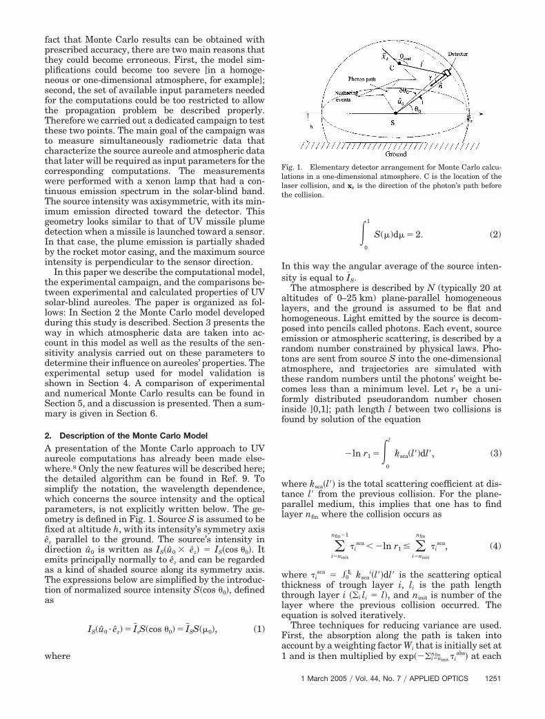
2. Description of the Monte Carlo Model

A presentation of the Monte Carlo approach to UVaureole computations has already been made else-where.8 Only the new features will be described here;the detailed algorithm can be found in Ref. 9. Tosimplify the notation, the wavelength dependence,which concerns the source intensity and the opticalparameters, is not explicitly written below. The ge-ometry is defined in Fig. 1. Source S is assumed to befixed at altitude h, with its intensity’s symmetry axisez parallel to the ground. The source’s intensity indirection u0 is written as IS�u0 � ez� � IS�cos �0�. Itemits principally normally to ez and can be regardedas a kind of shaded source along its symmetry axis.The expressions below are simplified by the introduc-tion of normalized source intensity S�cos �0�, definedas

IS(u0 · ez) � I�sS(cos �0) � I�SS(�0), (1)

where

�0

1

S(�)d� � 2. (2)

In this way the angular average of the source inten-sity is equal to I�S.

The atmosphere is described by N (typically 20 ataltitudes of 0–25 km) plane-parallel homogeneouslayers, and the ground is assumed to be flat andhomogeneous. Light emitted by the source is decom-posed into pencils called photons. Each event, sourceemission or atmospheric scattering, is described by arandom number constrained by physical laws. Pho-tons are sent from source S into the one-dimensionalatmosphere, and trajectories are simulated withthese random numbers until the photons’ weight be-comes less than a minimum level. Let r1 be a uni-formly distributed pseudorandom number choseninside ]0,1]; path length l between two collisions isfound by solution of the equation

�ln r1 ��0

l

ksca(l�)dl�, (3)

where ksca�l�� is the total scattering coefficient at dis-tance l= from the previous collision. For the plane-parallel medium, this implies that one has to findlayer nfin where the collision occurs as

�i�ninit

nfin�1

�isca � �ln r1 � �

i�ninit

nfin

�isca, (4)

where �isca � �0

li kscai�l��dl� is the scattering optical

thickness of trough layer i, li is the path lengththrough layer i ��i li � l�, and ninit is number of thelayer where the previous collision occurred. Theequation is solved iteratively.

Three techniques for reducing variance are used.First, the absorption along the path is taken intoaccount by a weighting factor Wi that is initially set at1 and is then multiplied by exp��i�ninit

nfin �iabs� at each

Fig. 1. Elementary detector arrangement for Monte Carlo calcu-lations in a one-dimensional atmosphere. C is the location of thelaser collision, and xk is the direction of the photon’s path beforethe collision.

1 March 2005 � Vol. 44, No. 7 � APPLIED OPTICS 1251

collision, where �iabs � �0

li kabsi�l��dl� is the absorption

optical thickness in layer i. Second, the probabilitythat the jth photon reaches the detector after k colli-sions is calculated at each scattering event by therelation

Hjk � P(cos �sca) �iexp��

0

dijk

kext(l)dl� S cos

��i

dijk�2,

(5)

where �sca is the virtual scattering angle between thephoton path and the detector direction, P�cos �sca� isthe scattering phase function in the layer where thecollision occurred, di

jk is the distance through layer ibetween the last collision and the detector ��i di

jk

� l�, � is the line-of-sight zenith angle, S is thedetector’s surface, and all the probabilities aresummed. The signal obtained thus converges to ex-actly the same results as in the classic method. How-ever, as the signal is not constrained to increase incomplete steps, convergence is achieved morequickly. Finally, the distribution of random numbersthat describe the source intensity is biased to in-crease the number of photons emitted in the directionclose to the symmetry axis. In that case, more pho-tons are launched in the sensor’s direction, so thedetected signal is higher, resulting in better statis-tics.

When the scattering point is located close to thedetector, the solid angle subtended by the detector’ssurface from the scattering point is no longer a dif-ferential element, and an integration must be per-formed. In this case we divide the detector intosmaller surfaces and sum the probabilities to reacheach elementary surface. At each scattering event,probability of detection Hjk and direction of photonarrival l, defined by angles � and �, respectively, arerecorded. During this step, the detector’s FOV is notrestricted, so � ranges from 0 to �.

The aureole can be characterized by the FOV’stransmittance, which is defined as the ratio of thetotal flux received by the detector (direct and scat-tered) to the flux that would be received in vacuum(direct signal without extinction). When the detectorhas a conical FOV of total angle �, the FOV’s trans-mittance is expressed as

T(�, �) � exp(��)

�

�j�1

Ntot

�l

�k�1

ncolj

WjkF(l; �)

(Ntot�4 ) ��0

�0��0 ��0

�0��0

S(cos ��)sin ��d��d��

, (6)

which is a generalization of relation (17) of Ref. 8 fora homogeneous atmosphere. In that equation, �� kext

sd is the optical thickness between the sourceand the sensor, both located in layer s, NT is the total

number of photons sent from the source, ncolj is thetotal number of collisions suffered by the jth photon,Wjk is the jth photon’s weight just after the kth colli-sion, and F�l; �� is a function introduced to delimitthe detector’s FOV and defined by F�l; �� 1 if l

� ��2 and F�l; �� 0 otherwise. The first term inthe FOV’s definition of the transmittance representsthe direct signal, and the second is the aureole’s con-tribution. One can also introduce the radianceB��, , �� in direction v � v�, �� (Fig. 2), whichobeys the following relation:

T(�, �) � exp(��) �d2

I�SS(cos �0)

��0

2 �0

��2

B(�, , �)|cos | sin

� dd�, (7)

where d is the source–sensor distance. We can obtainB��, , �� by deriving the FOV’s transmittance withrespect to angles � and �. However, it can be shownthat the radiance B��, , �� that is due to first-orderscattering is singular in the source direction �sin � 0�, as is the radiance that is due to a point source.4Despite this singularity, the introduction of radianceis still a convenient way to solve the radiative trans-fer problem. In fact, the overall source seen from thedetector may be considered an extended source be-cause of the scattering aureole. We remove this sin-gularity by defining the apparent radianceN��, , �� sr�1� as

N(�, , �) �d2 sin

I�S

B(�, , �). (8)

During our experiments the aureole is recorded byuse of an imaging sensor. Its sensitivity is high

Fig. 2. Definition of the detection direction geometry; (�, �) is thedirection of photon arrival in spherical coordinates.


enough that the sensor can detect the signal in direc-tions off the source. However, the FOV is not suffi-ciently wide for the sensor to record the whole aureolewith only one pointing. So we used horizontal andvertical scanning with various discrete lines of sight.The aureole was then characterized by the averageflux density inside a fraction of a ring, as shown inFig. 3. As we decided to compare quantities as closelyas possible with experimental results, the MonteCarlo outputs are processed to represent the recordedflux density. It must be stressed that this flux densityis different from the one that would be obtained by alarge-FOV sensor always looking in the source direc-tion. In our computations the zenith angle � in rela-tion (5) is relative to the average detector direction,which may be different from the source direction. If�p��, p, �p� denotes the photon flux [photon s�1] re-corded on pixel p, the total flux density ��, � (pho-ton s�1 pixel�1) is expressed by

�(�, ) �1

Npix�p�1

Npix

�p(�, p, �p), (9)

where the sum is taken over all pixels that belong tothe fraction of the ring that corresponds to zenithangle �. Experimentally, �p

exp��, p, �p� is directlyrecorded by the detector. �p

th��, p, �p� given by theMonte Carlo model is also calculated from the cal-culated apparent radiance Np��, p, �p�. A calibra-tion with the source at a short distance from thedetector is also performed to convert the MonteCarlo results into the same units as the experimen-tal results:

�pth(�, p, �p) � Np(�, p, �p)

��ref

S(�0 � 0) �dref

d �2 �p cos p

sin p,

(10)

where �ref is the total photon flux recorded by thedetector when it looks directly at the source and whendistance dref between the source and the detector issufficiently small that the scattered contribution isnegligible, and where �p is the FOV of pixel p. In thetwo last-named steps, first the computed results areconvoluted by the detector’s point-spread functionand then the radiance is calculated for differentwavelengths and integrated over the detector’s spec-tral band.

3. Input Data and Sensitivity Analysis

The atmosphere is assumed to be a plane-parallelmedium with typically 20 user-defined layers. Eachlayer interface is defined by a set of meteorologicalparameters such as pressure, temperature, aerosols,and molecular concentrations; their dependence onaltitude inside a layer is assumed to be linear. As thesource and the sensor are located only a few metersabove the ground, the atmospheric properties are de-scribed only from 0 to 25 km. The ground is assumedto be plane and homogeneous, with a Lambertian re-flectivity.

Rayleigh scattering cross sections and phasefunctions are calculated according to Bucholtz da-ta.10 The atmospheric gases that have the largestabsorption cross sections in the UV solar-blind bandare ozone, molecular oxygen, sulfur dioxide, andnitrogen dioxide. Generally, the absorption is dom-inated by ozone. However, near 240 nm, the oxy-gen’s absorption coefficient (Herzberg continuum)becomes of the same order of magnitude as theozone absorption coefficient calculated for a30�parts�in�109 by volume (ppbv) concentration.Close to 280 nm, sulfur dioxide can also be a non-negligible absorber for concentrations typicallyhigher than 20 ppbv. Absorptions for all these com-ponents are taken into account in our Monte Carlocomputations by use of cross-section data from re-cent laboratory measurements. UV absorption fromaerosols is generally less than from molecules, ex-cept in highly polluted urban climates. Aerosols’optical properties come either from the OpticalProperties of Aerosols and Clouds15 (OPAC) data-base or from measurements.

Before the experiments, we undertook systematicsensitivity calculations to determine the parame-ters that were most sensitive to the aureole’s prop-erties.16 The results were later used as a guide forselection of the set of meteorological parameters tobe accurately known during the field measure-ments. The sensitivity calculations were performedfor conditions close to those of the experiments: (1)the distance between source and sensor varied from500 to 4000 m, (2) source and sensor were located 1 mabove a flat ground, (3) the wavelength considered�280 nm� was close to the instrument’s maximumspectral response, and (4) the source intensity’s an-gular dependence was modeled by the simplifiedfunction8

Fig. 3. Discrete lines of sight for horizontal and vertical scanningand surfaces used to estimate the flux density onto a receiverversus pointing direction.


I(cos �0) � IS�

�2

1 � �S�(�S � 1)1�2 arcsin(�S � 1)��S�1�2

� (cos2 �0 � �S sin2 �0)1�2 �S � 1, (11)

with �S � 100, which corresponds to a shaded sourcetoward the observer. This model is useful because thesource intensity is defined with only one parameter,�S.

The most important input parameter is the ozoneconcentration at ground level. Ozone absorptionhas similar effects on FOV transmittance and directtransmittance.16 In the meantime, there is no sig-nificant effect of variation in ozone concentrationwith altitude on the aureole’s properties recorded1 m above the ground. A uniform profile with themeasured ozone concentration at ground level is suf-ficient for all computations. The second most impor-tant parameter is the aerosol extinction coefficient atground level. Meanwhile, Fig. 4 shows that detailedknowledge of the aerosol scattering phase function isgenerally not essential for prediction of the aureole’scharacteristics for this spectral domain. We workedout the FOV’s transmittance by using three differentaerosol phase functions calculated from Mie scatter-ing, which corresponded to maritime aerosols, urbanaerosols, and fog, and a modified Henyey–Greensteinphase function.4 We performed the computations byassuming purely scattering aerosols, to amplify thepotential differences between cases, and the sameoptical depth. The FOV’s transmittance exhibits thesame behavior for the Henyey–Greenstein phasefunction as for the phase functions that describe mar-itime or urban aerosols, despite the large differencesbetween phase functions in the forward-scatteringdirection (Fig. 5). The only curve that deviates fromthe average trend is that for fog. The maximum dif-ference reaches 25% for a 2° FOV and a source–sensor distance of 4 km. For small FOV angles the

most important contribution to the transmittancecomes from single-scattered photons. The forwardpeak observed in the fog’s phase function then has agreat influence on the transmittance results. For aFOV above 20°, multiple scattering becomes moresignificant and photons are affected by higher anglescattering. In that case the difference between thephase functions becomes less significant and the FOVtransmittance curves show a similar behavior for thefour aerosol types. The ratio of first-order scatteringto higher-order scattering is quite small in our case,because the source intensity is minimum toward theobserver. Similar calculations, performed for an iso-tropic source emission, show that the FOV’s trans-mittance becomes much more sensitive to the shapeof the phase function. In the case of a shaded source,the scattering phase function has to be known indetail only in special atmospheric conditions that cor-respond to narrow-peaked phase functions, such as infog or cloud. The FOV transmittance that corre-sponds to a shaded source in a moderately clear at-mosphere is not highly sensitive to the aerosols’scattering phase function, and there is no need tomeasure such a phase function when one is carryingout FOV transmittance experiments.

4. Experimental Setup

The campaign was performed from 21 to 28 March2001 inside Centre d’Essais en Vol airfield test centerin Brétigny, close to Paris. This location was selectedbecause it offers the opportunity to perform measure-ments for sufficiently large distances and to get me-teorological measurements. There were three mobilestations, one each dedicated to UV source manage-ment, optical measurements, and aerosol and mete-orological measurements.

A. UV Source and Detection System

The UV source was a 150�W xenon lamp, free of anyhousing, with the discharge tube mounted in the hor-izontal position. Its axis was aligned with the optical

Fig. 4. Comparison of FOV transmittance calculated for four scat-tering phase functions and two source–sensor distances. The cor-responding phase functions are plotted in Fig. 5.

Fig. 5. (a) Comparison of three aerosol phase functions from theOPAC database: urban �g � 0.629�, maritime �g � 0.689�, fog �g� 0.869�, and modified Henyey–Greenstein as defined by Eq. (27)of Ref. 4 with g � 0.72 and f � 0.5. (b) Details of the forward peaks.


sensor direction, so its minimum emission was di-rected toward the optical device. Figure 6 shows apolar plot of the source intensity recorded at a smalldistance from the detector, where atmospheric scat-tering effects were negligible. As a first approxima-tion, we considered the source axisymmetric, withparameter � equal to 3000.

The weak UV signal from the aureole was recordedby an imaging photon detector working in photon-counting mode. This sensor has been described else-where,17 and only the essential features are givenhere. It consisted of a UV filter, an objective lens (f� 105 mm, f�4.5), and a detector. The detector wascomposed of a RbCsTe photocathode, a stack of fourmicrochannel plates, and a resistive anode. Each UVphoton converted to a photoelectron gave rise to foursignals on the corners of the resistive anode, fromwhich the photon location was calculated. Each eventwas also time tagged, so an image could later bereconstructed. The optical filter was designed to re-ject near-UV and visible light, so the signal recordedwhen the sensor was looking directly toward the Sunat noon was smaller than the dark current (2.5 eventss�1). Thus the imaging photon detector is a highlysensitive device that is able to record the UV aureolefrom an outdoor artificial source in photon-countingmode, even in daylight.

B. Atmospheric Measurements

A rather comprehensive set of meteorological andaerosol properties was measured with the instru-

ments listed in Table 1. The equipment provided dif-ferent possibilities for investigating atmosphericaerosols by use of in situ measurements. All thesemeasurements were used to assess the aerosol extinc-tion coefficient at ground level, first in the visiblespectrum and then in the UV domain.

1. Optical MeasurementsA three-wavelength nephelometer was used in the

mobile station to measure the aerosol scattering co-efficient at 450, 550, and 700 nm in a 7°–170° rangeof scattering angle.18 The instrument was used inambient relative humidity without heating. Themean relative uncertainty of this instrument was as-sumed to be less than 5% (Ref. 19) and was duemainly to residual heating that modifies the relativehumidity inside the instrument. In dry conditions,the relative uncertainty after calibration was of theorder of 1% on the scattering coefficient.

2. Size DistributionThe size distribution of atmospheric aerosol was re-

trieved from the coupling between the optical analyz-ers that contribute to the partition function of theaerosol number in nine classes from 7 nm to 5 �m indiameter. The number concentrations of submicrome-ter particles were measured with a 3022A CPC partic-ulate counter of TSI company. All particles within adiameter size range from 0.007 to 3 �m were detected,with a 100% efficiency for 0.02 �m. A relative uncer-tainty of 5% has been calculated for the retrieved par-ticulate concentration.20 We also used twocomplementary types of optical particle size: KC18(Rion Company, Ltd., Japan) and MetOne 237 (Met-One Company). The KC18 sizer gives access to thepartition function of the aerosol in five diameterclasses (�0.10 �m, �0.15 �m, �0.20 �m, �0.30 �m,and �0.50 �m). The light source was a He–Ne laserat 663 nm, and the measurement was performed at a90° scattering angle. The inlet air flux rate was0.30 L�min. The MetOne instrument gives the aerosolpartition function in five diameter classes (�0.30,�0.50, �0.70, �1.00, �2.00, and �3.00 �m) but usesa diode laser source with an inlet flux rate of2.83 L�min.

3. Chemical AnalysesBlack carbon (BC) is the major contributor to ab-

sorption in urban and suburban areas. The BC con-centration was recorded continuously with anaethalometer (Model Magee Scientific, AE-14). Thisinstrument, calibrated with a constant value of19 m2 g�1 validated from chemical analysis per-formed on filters, is sensitive to the light-absorbentpart of the aerosols.21 The aethalometer measure-ment is representative for air masses affected by an-thropogenic pollution.22 The relative uncertainty inthe measurements of BC concentration performedwith this instrument was close to 10% after calibra-tion. At a longer sampling-time period (Table 1), aero-sol samples devoted to carbonaceous analyses werecollected with a low volume sampler �3 m3�h� on pre-

Fig. 6. Polar plot of the UV source’s angular intensity recorded ata small distance from the detector and best fit with Eq. (11) and� � 3000; (a) linear scale, (b) logarithmic scale.


viously cleaned Whatman glass-fiber filters. Carbonmass was determined by a thermal protocol (BC andorganic carbon). The precision of results is estimatedto be of the order of 10%.23 The accuracy of themethod was close to 20% and was linked to thermalseparation of BC and organic carbon for the range ofconcentrations that were observed in this study.24

Nuclepore membranes were used in parallel forweighing and measurement of major soluble ions byion chromatography. The membranes were mountedon stack filters to separate the coarse and the finefractions of the aerosol: The size cut was of the orderof 2 �m in diameter. Total particulate matter wasobtained with an absolute accuracy of 5 �g in a con-trolled environment with a relative humidity of lessthan 30%. The precision in ion chromatography re-sults was evaluated to be 10%.

Note that, because of the absorption properties ofozone in the Huggins band, its concentration wasmeasured simultaneously with its aerosol propertieson board the mobile aerosol station. The precision ofthe measurement was close to 5% after calibration.

5. Results and Discussion

A. Atmospheric Properties

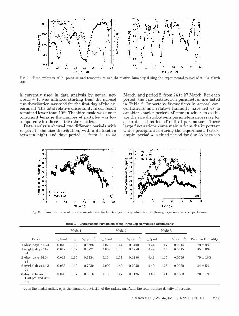
A first general idea of the meteorological conditionsduring the campaign is given by Fig. 7, where pres-

sure, temperature, and relative humidity are pre-sented. One can notice that the campaign wasconducted in a low-pressure situation, with maxi-mum pressures of �1010 hPa and an average value of�1000 hPa. The temperature never exceeded 17 °C.The relative humidity varied from 65% to 98%, andprecipitation occurred during the week. The dailyevolution of relative humidity was quite pronounced,with minima taking place in the middle of the dayfollowed by a progressive increase to reach a maxi-mum in the middle of the night. Ozone concentrationsrecorded during the five days on which scatteringexperiments took place are presented in Fig. 8. Theaverage ozone concentration reached 40 ppbv for 4days and was lower by a factor of 2 on March 26. Thisdecrease in ozone concentration directly affected theabsorption coefficient and the single-scattering al-bedo. Finally, the ozone measurements, which wererepeated every minute, showed significant temporalfluctuations during short periods. The ozone concen-tration variation that occurred during 1 h could reach30%.

The aerosol size distribution was continuously cal-culated from particle sizer measurements (Table 1)on 21–28 March. Trimodal distribution of a log-normal type was fitted by a Bayesian approach withconvergence of the stochastic gradient. This method

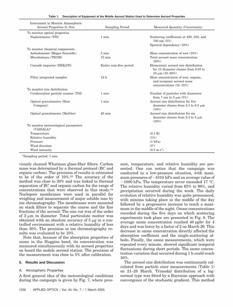
Table 1. Description of Equipment at the Mobile Aerosol Station Used to Determine Aerosol Properties

Instrument to Monitor AtmosphericAerosol Properties In Situ Sampling Period Measured Quantity (Uncertainty)

To monitor optical propertiesNephelometer (TSI) 1 min Scattering coefficients at 450, 550, and

700 nm (5%)Spectral dependency (10%)

To monitor chemical componentsAethalometer (Magee Scientific) 5 min Mass concentration of soot (10%)Microbalance (TEOM) 15 min Total aerosol mass concentration

(20%)Cascade impactor (DEKATI) Entire rain-free period Elementary aerosol size distribution

for 13 diameter classes from 0.03 to10 �m (10–20%)

Filter integrated samples 12 h Mass concentration of soot, organic,and inorganic aerosol massconcentrations (10–15%)

To monitor size distributionCondensation particle counter (TSI) 1 min Number of particles with diameters

from 7 nm to 3 �m (5%)Optical granulometer (Rion

Company)1 min Aerosol size distribution for five

diameter classes from 0.1 to 0.5 �m(10%)

Optical granulometer (MetOne) 45 min Aerosol size distribution for sixdiameter classes from 0.3 to 5 �m(10%)

To monitor meteorological parameters(VAISALA)a

Temperature �0.1 K�Relative humidity (1%)Pressure �1 hPa�Wind direction (5°)Wind intensity �0.5 m s1�

aSampling period, 1 min.


is currently used in data analysis by neural net-works.25 It was initiated starting from the aerosolsize distribution assessed for the first day of the ex-periment. The total relative uncertainty in our resultremained lower than 10%. The third mode was underconstraint because the number of particles was lowcompared with those of the other modes.

Data analysis showed two different periods withrespect to the size distribution, with a distinctionbetween night and day: period 1, from 21 to 23

March, and period 2, from 24 to 27 March. For eachperiod, the size distribution parameters are listedin Table 2. Important fluctuations in aerosol con-centrations and relative humidity have led us toconsider shorter periods of time in which to evalu-ate the size distribution’s parameters necessary foraccurate estimation of optical parameters. Theselarge fluctuations come mainly from the importantwater precipitation during the experiment. For ex-ample, period 3, a third period for day 26 between

Fig. 7. Time evolution of (a) pressure and temperature and (b) relative humidity during the experimental period of 21–28 March2001.

Fig. 8. Time evolution of ozone concentration for the 5 days during which the scattering experiments were performed.

Table 2. Characteristic Parameters of the Three Log-Normal Size Distributionsa

Period

Mode 1 Mode 2 Mode 3

Relative Humidityrm ��m� �g N0 ��m�3� rm ��m� �g N0 ��m�3� rm ��m� �g N0 ��m�3�

1 (day) days 21–24 0.029 1.32 0.8586 0.076 1.44 0.1400 0.44 1.27 0.0014 79 � 9%1 (night) days 21–

240.017 1.52 0.6227 0.057 1.76 0.3758 0.49 1.05 0.0015 85 � 6%

2 (day) days 24.3–27

0.029 1.85 0.8734 0.13 1.37 0.1230 0.42 1.15 0.0036 79 � 10%

2 (night) days 24.3–27

0.032 1.42 0.7930 0.092 1.49 0.2050 0.49 1.05 0.0020 84 � 5%

3 day 26 between1:40 pm and 3:50pm

0.026 1.97 0.8816 0.13 1.27 0.1125 0.38 1.21 0.0059 70 � 1%

arm is the modal radius, �g is the standard deviation of the radius, and N0 is the total number density of particles.


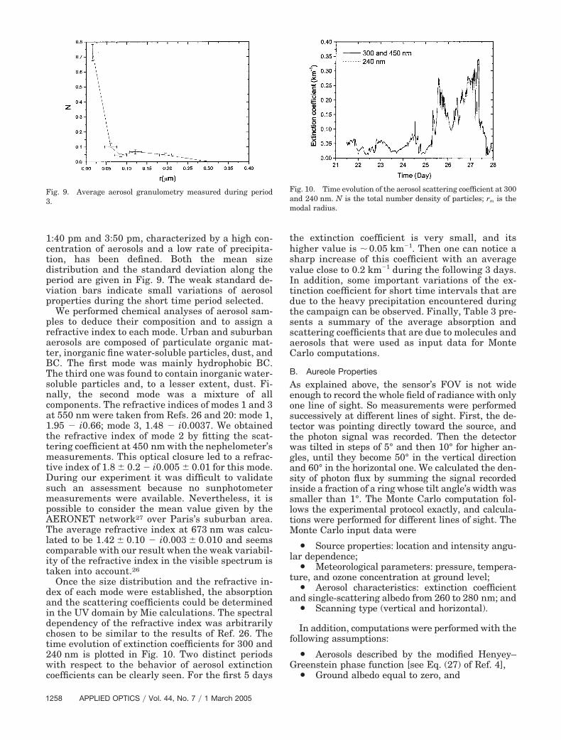
1:40 pm and 3:50 pm, characterized by a high con-centration of aerosols and a low rate of precipita-tion, has been defined. Both the mean sizedistribution and the standard deviation along theperiod are given in Fig. 9. The weak standard de-viation bars indicate small variations of aerosolproperties during the short time period selected.

We performed chemical analyses of aerosol sam-ples to deduce their composition and to assign arefractive index to each mode. Urban and suburbanaerosols are composed of particulate organic mat-ter, inorganic fine water-soluble particles, dust, andBC. The first mode was mainly hydrophobic BC.The third one was found to contain inorganic water-soluble particles and, to a lesser extent, dust. Fi-nally, the second mode was a mixture of allcomponents. The refractive indices of modes 1 and 3at 550 nm were taken from Refs. 26 and 20: mode 1,1.95 � i0.66; mode 3, 1.48 � i0.0037. We obtainedthe refractive index of mode 2 by fitting the scat-tering coefficient at 450 nm with the nephelometer’smeasurements. This optical closure led to a refrac-tive index of 1.8 � 0.2 � i0.005 � 0.01 for this mode.During our experiment it was difficult to validatesuch an assessment because no sunphotometermeasurements were available. Nevertheless, it ispossible to consider the mean value given by theAERONET network27 over Paris’s suburban area.The average refractive index at 673 nm was calcu-lated to be 1.42 � 0.10 � i0.003 � 0.010 and seemscomparable with our result when the weak variabil-ity of the refractive index in the visible spectrum istaken into account.26

Once the size distribution and the refractive in-dex of each mode were established, the absorptionand the scattering coefficients could be determinedin the UV domain by Mie calculations. The spectraldependency of the refractive index was arbitrarilychosen to be similar to the results of Ref. 26. Thetime evolution of extinction coefficients for 300 and240 nm is plotted in Fig. 10. Two distinct periodswith respect to the behavior of aerosol extinctioncoefficients can be clearly seen. For the first 5 days

the extinction coefficient is very small, and itshigher value is � 0.05 km�1. Then one can notice asharp increase of this coefficient with an averagevalue close to 0.2 km�1 during the following 3 days.In addition, some important variations of the ex-tinction coefficient for short time intervals that aredue to the heavy precipitation encountered duringthe campaign can be observed. Finally, Table 3 pre-sents a summary of the average absorption andscattering coefficients that are due to molecules andaerosols that were used as input data for MonteCarlo computations.

B. Aureole Properties

As explained above, the sensor’s FOV is not wideenough to record the whole field of radiance with onlyone line of sight. So measurements were performedsuccessively at different lines of sight. First, the de-tector was pointing directly toward the source, andthe photon signal was recorded. Then the detectorwas tilted in steps of 5° and then 10° for higher an-gles, until they become 50° in the vertical directionand 60° in the horizontal one. We calculated the den-sity of photon flux by summing the signal recordedinside a fraction of a ring whose tilt angle’s width wassmaller than 1°. The Monte Carlo computation fol-lows the experimental protocol exactly, and calcula-tions were performed for different lines of sight. TheMonte Carlo input data were

Y Source properties: location and intensity angu-lar dependence;

Y Meteorological parameters: pressure, tempera-ture, and ozone concentration at ground level;

Y Aerosol characteristics: extinction coefficientand single-scattering albedo from 260 to 280 nm; and

Y Scanning type (vertical and horizontal).

In addition, computations were performed with thefollowing assumptions:

Y Aerosols described by the modified Henyey–Greenstein phase function [see Eq. (27) of Ref. 4],

Y Ground albedo equal to zero, and

Fig. 9. Average aerosol granulometry measured during period3.

Fig. 10. Time evolution of the aerosol scattering coefficient at 300and 240 nm. N is the total number density of particles; rm is themodal radius.


Y Homogeneous ozone and aerosol concen-trations.

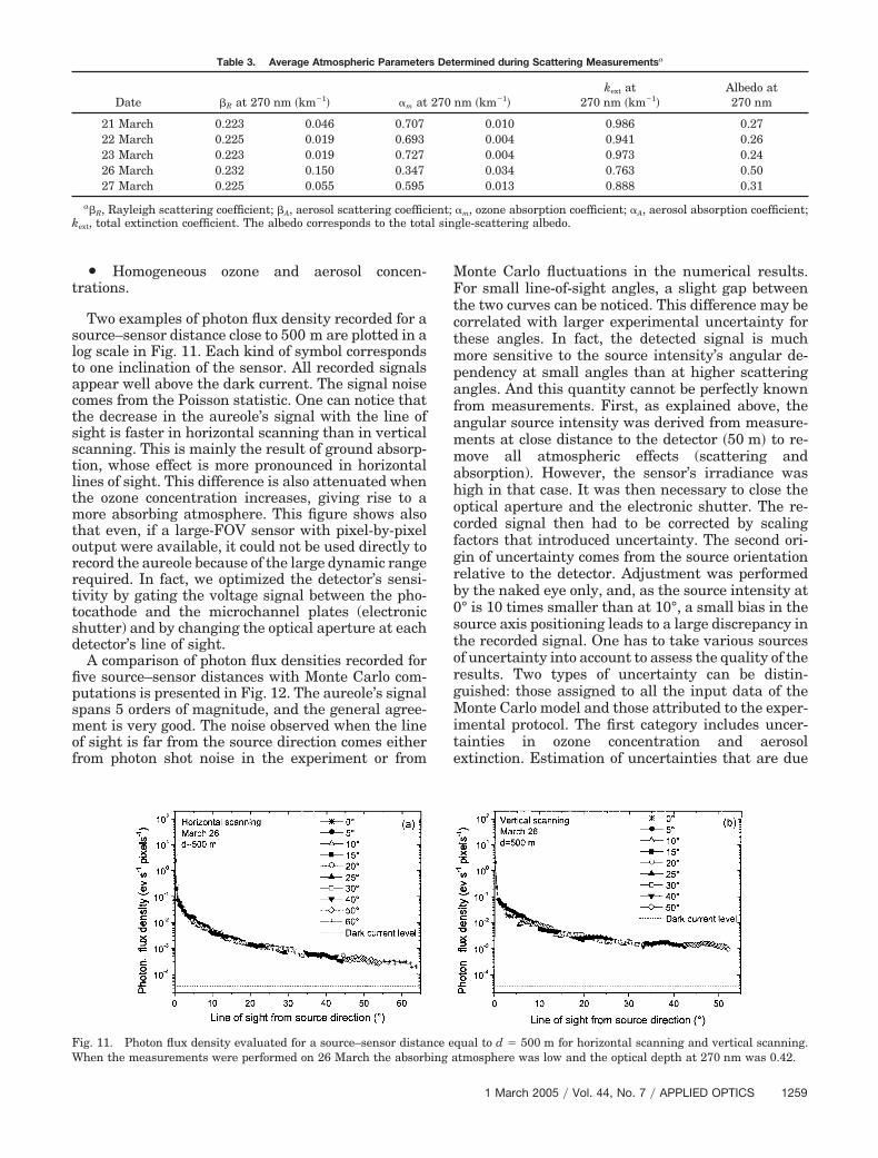
Two examples of photon flux density recorded for asource–sensor distance close to 500 m are plotted in alog scale in Fig. 11. Each kind of symbol correspondsto one inclination of the sensor. All recorded signalsappear well above the dark current. The signal noisecomes from the Poisson statistic. One can notice thatthe decrease in the aureole’s signal with the line ofsight is faster in horizontal scanning than in verticalscanning. This is mainly the result of ground absorp-tion, whose effect is more pronounced in horizontallines of sight. This difference is also attenuated whenthe ozone concentration increases, giving rise to amore absorbing atmosphere. This figure shows alsothat even, if a large-FOV sensor with pixel-by-pixeloutput were available, it could not be used directly torecord the aureole because of the large dynamic rangerequired. In fact, we optimized the detector’s sensi-tivity by gating the voltage signal between the pho-tocathode and the microchannel plates (electronicshutter) and by changing the optical aperture at eachdetector’s line of sight.

A comparison of photon flux densities recorded forfive source–sensor distances with Monte Carlo com-putations is presented in Fig. 12. The aureole’s signalspans 5 orders of magnitude, and the general agree-ment is very good. The noise observed when the lineof sight is far from the source direction comes eitherfrom photon shot noise in the experiment or from

Monte Carlo fluctuations in the numerical results.For small line-of-sight angles, a slight gap betweenthe two curves can be noticed. This difference may becorrelated with larger experimental uncertainty forthese angles. In fact, the detected signal is muchmore sensitive to the source intensity’s angular de-pendency at small angles than at higher scatteringangles. And this quantity cannot be perfectly knownfrom measurements. First, as explained above, theangular source intensity was derived from measure-ments at close distance to the detector �50 m� to re-move all atmospheric effects (scattering andabsorption). However, the sensor’s irradiance washigh in that case. It was then necessary to close theoptical aperture and the electronic shutter. The re-corded signal then had to be corrected by scalingfactors that introduced uncertainty. The second ori-gin of uncertainty comes from the source orientationrelative to the detector. Adjustment was performedby the naked eye only, and, as the source intensity at0° is 10 times smaller than at 10°, a small bias in thesource axis positioning leads to a large discrepancy inthe recorded signal. One has to take various sourcesof uncertainty into account to assess the quality of theresults. Two types of uncertainty can be distin-guished: those assigned to all the input data of theMonte Carlo model and those attributed to the exper-imental protocol. The first category includes uncer-tainties in ozone concentration and aerosolextinction. Estimation of uncertainties that are due

Table 3. Average Atmospheric Parameters Determined during Scattering Measurementsa

Date �R at 270 nm �km�1� �m at 270 nm �km�1�kext at

270 nm �km�1�Albedo at270 nm

21 March 0.223 0.046 0.707 0.010 0.986 0.2722 March 0.225 0.019 0.693 0.004 0.941 0.2623 March 0.223 0.019 0.727 0.004 0.973 0.2426 March 0.232 0.150 0.347 0.034 0.763 0.5027 March 0.225 0.055 0.595 0.013 0.888 0.31

a�R, Rayleigh scattering coefficient; �A, aerosol scattering coefficient; �m, ozone absorption coefficient; �A, aerosol absorption coefficient;kext, total extinction coefficient. The albedo corresponds to the total single-scattering albedo.

Fig. 11. Photon flux density evaluated for a source–sensor distance equal to d � 500 m for horizontal scanning and vertical scanning.When the measurements were performed on 26 March the absorbing atmosphere was low and the optical depth at 270 nm was 0.42.


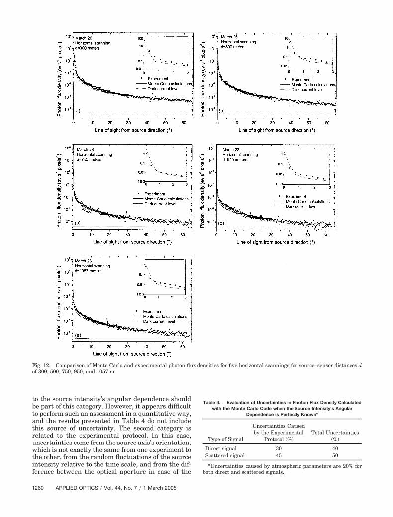
to the source intensity’s angular dependence shouldbe part of this category. However, it appears difficultto perform such an assessment in a quantitative way,and the results presented in Table 4 do not includethis source of uncertainty. The second category isrelated to the experimental protocol. In this case,uncertainties come from the source axis’s orientation,which is not exactly the same from one experiment tothe other, from the random fluctuations of the sourceintensity relative to the time scale, and from the dif-ference between the optical aperture in case of the

Fig. 12. Comparison of Monte Carlo and experimental photon flux densities for five horizontal scannings for source–sensor distances dof 300, 500, 750, 950, and 1057 m.

Table 4. Evaluation of Uncertainties in Photon Flux Density Calculatedwith the Monte Carlo Code when the Source Intensity’s Angular

Dependence is Perfectly Knowna

Type of Signal

Uncertainties Causedby the Experimental

Protocol (%)Total Uncertainties

(%)

Direct signal 30 40Scattered signal 45 50

aUncertainties caused by atmospheric parameters are 20% forboth direct and scattered signals.


reference measurement �50 m� and the scatteringmeasurements. Figure 12 shows that the gap be-tween experimental and theoretical results is in gen-eral largely within the error bars, except at smallangles.

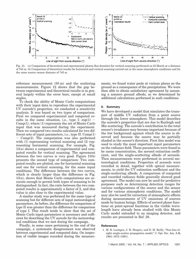
To check the ability of Monte Carlo computationswith their input data to reproduce the experimentalUV aureole’s properties, we conducted a sensitivityanalysis. It was based on two types of comparison.First we compared experimental and computed re-sults in the same situation, i.e., type I: exp(1) �Comp(1), where (1) represents the set of Monte Carloinput that was measured during the experiment.Then we compared two results calculated for two dif-ferent sets of input parameters, i.e., type II: Comp(1)� Comp(2). The computation was also performedwith (1) representing vertical scanning and (2) rep-resenting horizontal scanning. For example, Fig.13(a) shows a comparison of experimental and com-puted results for vertical scanning. The agreementbetween the two curves is very good. Figure 13(b)presents the second type of comparison: Two com-puted results are plotted, one for horizontal scanningand one for vertical scanning, for the same inputconditions. The difference between the two curves,which is clearly larger than the difference in Fig.13(a), shows that Monte Carlo computations are ac-curate enough to permit both types of scanning to bedistinguished. In fact, the ratio between the two com-puted results is approximately a factor of 2, and thisvalue is also close to the experimental value.

A similar study was performed for the same type ofscanning but for different sets of input meteorologicalparameters. As before, the difference for comparison oftype II was greater than the difference for comparisonof type I. This result tends to show that the set ofMonte Carlo input parameters is necessary and suffi-cient for describing the UV aureole for the meteorolog-ical conditions that we met during the campaign.

Finally, in some cases pertaining to the end of thecampaign, a systematic disagreement was observedbetween experimental and computed data. On inspec-tion of visible images recorded during the measure-

ments, we found water pools at various places on theground as a consequence of the precipitation. We werethen able to obtain satisfactory agreement by assum-ing a nonzero ground albedo, as we determined byadditional calculations performed in such conditions.

6. Summary

We have developed a model that simulates the trans-port of middle UV radiation from a point sourcethrough the lower atmosphere. This model describesthe aureole’s properties that are due to Rayleigh andMie scattering. The aureole’s contribution to the totalsensor’s irradiance may become important because ofthe low background against which the source is ob-served and because the source may be partiallyshaded in the sensor’s direction. First this model wasused to study the most important input parameterson the radiance field. These parameters were found tobe ozone concentration, the aerosol extinction coeffi-cient, and the single-scattering albedo of aerosols.Then measurements were performed in several me-teorological conditions. Properties of aerosols wererecorded in detail, together with optical measure-ments, to yield the UV extinction coefficient and thesingle-scattering albedo. A comparison of computedand recorded radiance fields generally showed goodagreement. The model can now be used for predictivepurposes such as determining detection ranges forvarious configurations of the source and the sensorand for various atmospheric conditions. The modelmay also be used for correction of atmospheric effectsduring measurements of UV emissions of sourcesmade by human beings. Effects of aerosol phase func-tions on point-spread functions in the visible wave-length have already been studied with this MonteCarlo model extended to an imaging detector, andresults are presented in Ref. 28.

References1. M. R. Luettgen, J. H. Shapiro, and D. M. Reilly, “Non-line-of-

sight single-scatter propagation model,” J. Opt. Soc. Am. A 8,1964–1972 (1991).

Fig. 13. (a) Comparison of theoretical and experimental photon flux densities for vertical scanning performed on 23 March at a distanceof 745 m. (b) Comparison of theoretical results for horizontal and vertical scanning carried out in the same atmospheric conditions and forthe same source–sensor distance of 745 m.


2. M. Lindner, S. Elstein, and P. Lindner, “Solar blind and bispec-tral imaging with ICCD, BCCD and EBCCD cameras,” in Im-age Intensifiers and Applications, C. B. Johnson, T. D. Maclay,and F. A. Allahdadi, eds., Proc. SPIE 3434, 22–31 (1998).

3. D. Walker, V. Kumar, K. Mi, P. Sandvik, P. Kung, X. H. Zhang,and M. Razeghi, “Solar blind AlGaN photodiodes with very lowcutoff wavelength,” Appl. Phys. Lett. 76, 403–405 (2000).

4. A. S. Zachor, “Aureole radiance field about a source in a scattering–absorbing medium,” Appl. Opt. 17, 1911–1922 (1978).

5. F. Riewe and A. E. S. Green, “Ultraviolet aureole around asource at a finite distance,” Appl. Opt. 17, 1923–1929 (1978).

6. R. R. Meier, J. S. Lee, and D. E. Anderson, “Atmosphericscattering of middle UV radiation from an internal source,”Appl. Opt. 17, 3216–3225 (1978).

7. K. N. Liou, Y. Takano, S. C. Ou, A. Heymsfield, and W. Kreiss,“Infrared transmission through cirrus clouds: a radiativemodel for target detection,” Appl. Opt. 29, 1886–1896 (1990).

8. C. Lavigne, A. Roblin, V. Outters, S. Langlois, T. Girasole, andC. Rozé, “Comparison of iterative and Monte Carlo methods forcalculation of the aureole about a point source in the Earth’satmosphere,” Appl. Opt. 38, 6237–6246 (1999).

9. C. Lavigne, “Etude théorique et expérimentale de la propaga-tion du rayonnement UV dans la basse atmosphère, Ph.D.dissertation (Université de Rouen, Rouen, France, 2001).

10. A. Bucholtz, “Rayleigh-scattering calculations for the terres-trial atmosphere,” Appl. Opt. 34, 2765–2773 (1995).

11. J. P. Burrows, A. Dehn, B. Deters, S. Himmelmann, A. Richter,S. Voigt, and J. Orphal, “Atmospheric remote-sensing refer-ence data from GOME. 1. Temperature-dependent absorptioncross-sections of NO2 in the 231–794�nm range,” J. Quant.Spectrosc. Radiat. Transfer 60, 1025–1031 (1998).

12. J. P. Burrows, A. Richter, A. Dehn, B. Deters, S. Himmelmann,S. Voigt, and J. Orphal, “Atmospheric remote-sensing refer-ence data from GOME. 2. Temperature-dependent absorptioncross-sections of O3 in the 231–794 nm range,” J. Quant. Spec-trosc. Radiat. Transfer 61, 509–517 (1999).

13. A. C. Vandaele, P. C. Simon, J. M. Guilmot, M. Carleer, and R.Colin, “SO2 absorption cross-section measurement in the UVusing a Fourier transform spectrometer,” J. Geophys. Res. 99,25,599–25,605 (1994).

14. A. Jenouvrier, M. F. Mérienne, B. Coquart, M. Carleer, S.Fally, A. C. Vandaele, C. Hermans, and R. Colin, “Fouriertransform spectroscopy of the O2 Herzberg bands. I. Rotationalanalysis,” J. Mol. Spectrosc. 198, 136–162 (1999).

15. M. Hess, P. Koepke, and I. Schult, “Optical properties of aero-sols and clouds: The software package OPAC,” Bull. Am. Me-teorol. Soc. 79, 831–844 (1998).

16. C. Lavigne, P. Chervet, S. Langlois, and A. Roblin, “Atmo-spheric propagation model for calculation of the aureole abouta point source,” in Atmospheric Propagation, Adaptive Sys-tems, and Laser Radar Technology for Remote Sensing, J. D.Gonglewski, ed., Proc. SPIE 4167, 43–52 (2001).

17. C. Lavigne, A. Roblin, and S. Langlois, “Solar-blind UV imag-ing photon detector with automatic gain control,” Meas. Sci.Technol. 13, 713–719 (2002).

18. B. A. Bodhaine, N. C. Ahlquist, and R. C. Schnell, “Three-wavelength nephelometer suitable for aircraft measurementsof background aerosol scattering coefficient,” Atmos. Environ.10, 2268–2276 (1991).

19. P. Chazette, “The monsoon aerosol extinction properties atGoa during INDOEX as measured with lidar,” J. Geophys.Res., 108, 10.1029/2002JD002074 (2003).

20. P. Chazette and C. Liousse, “A case study of optical and chem-ical ground apportionment for urban aerosols in Thessaloniki,”Atmos. Environ. 35, 2497–2506 (2001).

21. A. D. A. Hansen and T. Novakov, “Real time measurementsof aerosol black carbon during the carbonaceous speciesmethods comparison study,” Aerosol Sci. Technol. 12, 194–199 (1990).

22. J. E. Penner, “Carbonaceous aerosols influencing atmosphericradiation: black and organic carbon,” in Report of the DahlemWorkshop on Aerosol Forcing of Climate, R. J. Charlson andJ. Heintzenberg, eds. (Wiley, New York, 1995), pp. 91–108.

23. H. Cachier, M. P. Brémond, and P. Buat-Ménard, “Determi-nation of atmospheric soot carbon with a simple thermalmethod,” Tellus 41B, 379–390 (1989).

24. M. P. Brémond, H. Cachier, and P. Buat-Ménard, “Particulatecarbon in the Paris region atmosphere,” Environ. Technol.Lett. 10, 339–346 (1989).

25. J. Hadji-Lazaro, C. Clerbaux, and S. Thiria, “An inversionalgorithm using neural networks to retrieve atmospheric COtotal columns from high-resolution nadir radiances,” J. Geo-phys. Res. 104, 23841–23854 (1999).

26. E. Volz, “Infrared refractive index of the atmospheric aerosolsubstances,” Appl. Opt. 11, 755–759 (1972).

27. B. N. Holben, T. F. Eck, I. Sluster, D. Tanré, J. P. Buis, A.Setzer, E. Vermote, J. A. Reagan, Y. J. Kaufman, T. Nakajima,F. Lavenu, I. Jankowiak, and Z. Smirnov, “AERONET—afederated instrument network and data archive for aerosolcharacterisation,” Remote Sens. Environ. 66, 1–16 (1998).

28. P. Chervet, C. Lavigne, A. Roblin, and P. Bruscaglioni, “Effectsof aerosol scattering phase function on point-spread-functioncalculations,” Appl. Opt. 41, 6489–6498 (2002).


Experimental and theoretical studies of the aureole about a point source that is due to atmospheric...

Documents

Transcript of Experimental and theoretical studies of the aureole about a point source that is due to atmospheric...