Experimental and modelled mechanical behaviour of a rock fracture under normal stress

$: Experimental and modelled mechanical behaviour of a rock fracture under normal stress$
Rock Mech Rock Engng (2008) 41: 869–892

DOI 10.1007/s00603-008-0166-y

Printed in The Netherlands

Experimental and modelled mechanical behaviourof a rock fracture under normal stress

By

A. Marache1, J. Riss1, S. Gentier2

1 Universit�ee Bordeaux 1, GHYMAC, Av. des Facult�ees, Talence Cedex, France2 BRGM, Orl�eeans Cedex, France

Received June 27 2007; Accepted January 11 2008; Published online April 3 2008# Springer-Verlag 2008

Summary

The mechanical and hydromechanical behaviour of isolated rock joints is of prime impor-tance for a correct understanding of the behaviour of jointed rock masses. This paper focuseson the mechanical behaviour of a fracture under normal stress (fracture closure), usingapproaches based on both experimentation and modelled analysis. Experimental closure testswere carried out by positioning four displacement transducers around a fracture, leading toresults which tended to vary as a function of transducer location. Such variations can beexplained by the non-constant void space distribution between both walls of the fracture. Thepresent study focuses on the importance of transducer location in such a test, and on thesignificant role played, in terms of mechanical response, by the morphology of the fracturesurfaces.

An analytical mechanical model is then developed, which takes into account the defor-mation of surface asperities and of the bulk material surrounding the fracture; it also includesthe effects of mechanical interaction between contact points. The model is validated bysimulating the behaviour which is very similar to experimental observations. Various paramet-ric studies (scale effect, spatial distribution of contact points) are then carried out. The studyof scale effects reveals a decrease in the normal stiffness with increasing fracture size. Finally,analysis of the role of various mechanical parameters has shown that the most influentialof these is Young’s modulus corresponding to the bulk material surrounding the joint. Manyapplications, such as geothermal fluid recovery from fractures, could benefit from theseresults.

Keywords: Fracture, mechanical behaviour, normal stress, experimental device, roughness,analytical model, parametric study

Correspondence: Antoine Marache, Universit�ee Bordeaux 1, GHYMAC, Av. des Facult�ees, 33405 TalenceCedex, Francee-mail: [email protected]

1. Introduction

In order to understand the mechanical and hydromechanical behaviour of fractured

rock masses, it is essential to study single fractures. Numerous applications could

benefit from the study of fractures at small scale. Some examples are geothermy, the

study of petroleum reservoirs and all other types of energy recovery. Furthermore, the

outcome of this study could be used to determine parameters needed by numerical

codes, such as used in various civil engineering applications, or for the determination

of rock mass stability.

The present paper focuses on the mechanical behaviour of a rock joint under

normal stress. This is the first step in the direction of a more global hydromechanical

study of single fractures (normal and shear behaviour). Fractures (or joints) can be

thought of as two rough surfaces in partial contact with one another, characterised by a

void space between opposite walls of the fracture. When the normal stress is in-

creased, progressive closure of the rock joint is observed, together with an increase

in contact area between both walls. This evolution plays a key role in the development

of flow paths through the fracture.

Our study is presented in two parts: the experimental approach, and the numeri-

cally modelled approach. In the first, the importance of the position of the displace-

ment transducer on the fracture is emphasised and illustrated using mechanical results.

In the second part of the paper, following a brief appraisal of relevant models found in

the literature, our model is presented. It is validated by comparing simulated results

with the experimental results found in the first part of the study. Lastly, various

applications of the model are described, such as the study of scale effects, the deter-

mination of fracture contact zones during a test, and the influence of mechanical

parameter variations on the test results.

2. Experimental study of the mechanical behaviour of a rock

fracture under normal stress

The fracture studied in this paper is located in mortar replicas of a granitic sample

(diameter 90 mm); such replicas were used because many shear tests needed to be

performed under various conditions, and this approach enabled the same fracture

surface morphology to be respected for each test. The replicas have a Young’s modu-

lus of 31 GPa, a Poisson’s ratio equal to 0.19 and a compressive strength of 75 MPa;

44% of the grains have a size ranging from 0.4 mm to 1.0 mm, and 28% are larger than

1 mm. In the following, the experimental procedures are presented, followed by de-

tailed analysis of the results.

2.1 Experimental procedures

The mechanical test used to study the behaviour of a rock fracture under normal stress

is normally performed with a uniaxial apparatus: a normal force is applied to the free

surface of the upper wall of the fracture which closes at a constant velocity. It should

be noted that the upper wall can move only in the vertical direction, and that all

870 A. Marache et al.

possible rotations of the free surface are inhibited by the test apparatus. Before

initiating the test, particular attention should be paid to two details: the transducer

position and the design of the load-unload cycles, in order to ensure that good match-

ing is achieved at both walls of the fracture.

2.1.1 Transducer position

The experimental device used by Flamand (2000) to perform mechanical tests com-

prises one force transducer and four displacement transducers (LVDT) located around

the fracture (Fig. 1). The h value (Fig. 1) is chosen to be as small as possible so that

the measurement is influenced predominantly by closure of the fracture, rather than by

deformations of the surrounding rock; here, the value of h is 26 mm. Nevertheless, the

influence of rock deformations is corrected, with the corrected closure �V of the

fracture being given by:

�V ¼ �Vmeasured ��N � h

Eð1Þ

where �Vmeasured is the measured displacement, E is Young’s modulus for the sample,

�N is the applied normal stress and h is the vertical distance (26 mm) separating the

two transducers.

2.1.2 Load-unload cycles before the test

The closure test of a fracture can be performed only if its two walls are matched

in-situ; this is why several load-unload cycles are needed before beginning the test.

Without this preliminary step, the test would be carried out under conditions of

matching fracture walls, but not of fracture deformations. Accurate experimental

procedures were described by Gentier (1986) in order to achieve such optimal

matching (Fig. 2). Several ‘‘sub-tests’’ are performed as follows: following applica-

tion of a pre-load (defined as the stress required to obtain initial closure of the

fracture with a small normal stiffness), three load-unload cycles are carried out with

Fig. 1. Position of displacement transducers (lateral and aerial views)

Mechanical behaviour of a rock fracture 871

the maximum normal stress being increased at each cycle, up to a level of 20 MPa

for the last cycle (between each cycle, the sample is unloaded down to the pre-load

stress); the pre-load is unloaded after the last cycle. After completion of one such

‘‘sub-test’’, irreversible residual closure of the fracture can be observed; this irre-

versible residual closure decreases as the number of ‘‘sub-tests’’ increases. When the

irreversible residual closure approaches zero, optimal matching of the walls has been

achieved; the sample’s behaviour then becomes reversible, characterised by hyster-

esis. In general, three sub-tests were needed for our samples to be optimally

matched.

Experimental results are presented in the next section; these are obtained from one

test performed according to the procedures described above (using 3 preliminary

‘‘sub-tests’’ before the true test) on a mortar replica of the granitic sample.

Fig. 2. Experimental procedure to obtain optimal matching of both walls


2.2 Experimental results

2.2.1 Global results

The four normal curves plotted in Fig. 3 (normal stress as a function of fracture

closure) correspond to the recordings of the four displacement transducers, with the

dashed line showing the average of the four transducer values.

These curves can be separated into two components: below and above 1 MPa,

which is the normal stress value used for pre-loading, as described in the previ-

ous section. This value was common to all transducers. The initial closure was

equal to 0.070 mm for transducers 1 to 3, and 0.095 mm for transducer 4. Beyond

this pre-load value, the same behaviour was observed for all the transducers,

with the same normal stiffness value (slope of the curve, 250 MPa=mm) for a

given normal stress. The recorded behaviour is thus the same for all the transdu-

cers, with a horizontal translation along the x-axis corresponding to a different

initial closure value for each transducer. The main conclusion is that initial closure

occurs more or less quickly, depending on which zone of the fracture is being

considered.

It can be seen obvious that the pre-load and normal stiffness values of the mean

curve are the same as those corresponding to each separate transducer. However,

although the initial mean closure is 0.075 mm, as seen previously this value varies

between transducers. If a single value is needed for this parameter, great care should

be taken because of the range observed between measuring points. The reasons for this

behaviour are provided in the following section.

Fig. 3. Measured normal stress as a function of fracture closure: trends for four different transducers, andmean curve


2.2.2 Explanation of differences between transducer measurements

With the deformation test of a rock fracture under normal stress conditions, leading to

closure of the void space, differences between measured values are due only to

variations in the morphology of the fracture surfaces. Because rotations of the upper

wall are inhibited, changes detected can only be explained by variations in the frac-

ture’s void height. Figure 4 shows a map of the cast mortar void space replica (Gentier

and Hopkins, 1997) and of the transducer locations; on this map, the lightest zones

correspond to largest voids (white zones represent a void of more than 0.20 mm).

It can be seen that the left side of the void space shows, on average, larger voids

than the right side; the greatest void heights are located near to transducer 4. In this

zone, greater vertical displacements are needed to achieve initial closure of the frac-

ture. Nevertheless, once this closure is reached, the same behaviour is recorded by all

the transducers.

Analysis of the data recorded during the described experiment has enabled classi-

cal fracture closure behaviour to be studied. One of the main conclusions of this study

is the importance of choosing the correct type of device for the test, and the significant

role of transducer location. These considerations are essential for correct modelling of

fracture closure phenomena under normal stress.

3. Modeling the mechanical behaviour of a rock fracture under normal stress

3.1 Bibliographical review

Many models have been developed to describe the mechanical behaviour of a rock

fracture under normal stress. These can be classified into three categories: empirical,

analytical and numerical models.

In the first of these, the model relies on the fitting of a non-linear mathematical

function (hyperbolic or logarithm for example) to an experimental curve. Input param-

Fig. 4. Void space map with transducer locations


eters vary as a function of the model: some models use the elasticity modulus (Shehata,

1971), the material constant (Goodman, 1976; Detournay, 1979; Bandis, 1980) or the

initial value of fracture closure (pre-load) (Goodman, 1976; Detournay, 1979). Only the

model of Brown and Scholz (1986) takes morphological characteristics into account. All

of these models rely on fits to experimental curves, but do not allow a mechanical

behaviour to be predicted. Furthermore, Bandis et al. (1983) established a relationship

between the JRC (Joint Roughness Coefficient) roughness parameter and mechanical

parameters such as maximum closure of the fracture, or normal stiffness. Nevertheless,

such a model makes use of parameters which can be obtained from experimental data

only. Because of the non-predictive nature of such models, other methods are needed.

A second class of models (analytical) was used in order to explicitly take into

account the morphology of the fracture surfaces: these models were designed to take

into account the stress-strain relationship between two rough, contacting surfaces.

Many models of this type require the fracture surface to be discretised into zones

characterised by asperities of varying height with respect to a reference plane. A given

asperity is characterised by its form, its height, its width and the height of the void

between it and the opposite surface. Models of this class are based on the principle of

computing the individual stresses applied when local asperities come into contact, in

order to compute the total stress on the fracture.

Of the various models of this type, it is of interest to note that developed by Tsang

and Witherspoon (1981), who proposed coupling a void deformation model (defor-

mation of an elliptic void, as described by Walsh, 1965) and the asperity deformation

model of Gangi (1978), which describes the contact between a smooth and a rough

surface. The drawback of this model is its reliance on empirical parameters; other

types of model, which do not rely on the use of such parameters, have been developed

in order to predict a fracture’s mechanical behaviour.

Another approach is to use Hertz’s (1882) equations, which describe the elastic

deformation of two contacting spheres. Historically, these were the first models which

required only the mechanical characteristics of the material and the morphology of the

fracture’s surfaces. The application of these models to rough surfaces is explained in

detail by Gentier (1986), who uses studies of the behaviour of steel developed by

Greenwood and Williamson (1966), and Greenwood and Tripp (1971). It has been

shown that for low and medium stress levels the predicted fracture closure is greater

than that measured experimentally, and that for high stress levels the normal stiffness

and the contact area between both walls are underestimated. Of the many other

authors who have used this approach, it is of interest to note the papers of Swan

(1983), Matsuki et al. (2001) and Lanaro (2001), where a model is proposed that takes

into account plasticity and the unloaded phase of the fracture.

When a normal test is performed, no damage is noted on the fracture surfaces.

Nevertheless, when the true stress acting on each contacting asperity (rather than on

the whole fracture) is calculated, the values obtained are found to be much greater than

the rock compression strength. Only asperity confinement can explain these observa-

tions. This interpretation has been included in Gentier’s (1986) model, which is

derived from that of Billaux and Feuga (1984). When this approach is compared with

previous models, the main difference observed is an improved agreement between

theoretical and experimental curves, for high levels of normal stress.


Another model is based on joint deformation analysis, which takes into account

both asperity deformations and deformations of the rock surrounding the asperities.

Two main classes of models respect this approach: those due to Cook (1992) based on

Hertz’s theory and on the superposition principle in linear elasticity respectively

(Timoshenko and Goodier, 1970) (the displacement of a zone is given by the sum of

all contributing elementary displacements); the latter approach was used by Hopkins

(1990) (it forms the basis of the model used in the present study, cf. Section 3.2), and

by Pyrak-Nolte and Morris (2000), Lee and Harrison (2001), Borri-Brunetto et al.

(1998, 2001) and Capasso (2000).

Finally, the last category of models includes all those based on a numerical approach,

as for example is the case of the distinct element method. A comparison of various

numerical methods used for rock mass modelling can be found in Davias (1997).

3.2 Presentation of the model developed for the present study

The model presented in the following is based on the joint deformation approach and

was initially developed by Hopkins (1990, 2000), and later improved by Marache

(2002). We present the method used to represent the fracture, and then describe how

the computations are implemented. Improvements with respect to the initial model

include the possibility of modelling greater fracture sizes, and the inclusion of total-

force boundary conditions.

The model relies on an accurate description of the topography of the fracture walls

and of the void space. A geostatistical methodology was developed in order to obtain

topographical maps of the fracture surfaces from profile data (Marache et al., 2002).

Fractures are modelled as the interface between two elastic half spaces. The surface

roughness of the interface walls is modelled by discretizing the surface topography

maps into a grid of elements. Each element thus represents an asperity on the elastic

half space. In order to correctly evaluate the normal stress levels, asperities are rep-

resented by cylinders of radius R, with the height H of each cylinder being determined

from the void space map (Fig. 5). In addition, the material’s mechanical properties, i.e.

Young’s modulus (E) and Poisson’s ratio (�), are required. Different material proper-

ties can be assigned to each of the two half spaces and to each of the asperity subsets.

This is important for cases in which surface asperities are likely to be weaker than the

Fig. 5. Modelling of joint surfaces


surrounding rock because of geologic processes; as an example, fluid flow through

fractures can alter the surfaces it encounters.

Fractures can be thought of as two rough surfaces in partial contact. The model

presented in the following is based on the computation of forces acting between both

fracture walls, at each contact zone, for a specified applied normal load. One of our

main objectives was to derive an analytical formulation which enables the normal

stresses acting on contact areas to be determined, for a given value of normal dis-

placement (or which enables the resulting displacements to be predicted for a specified

applied load). Because elastic behaviour is assumed under normal loading (the normal

stress applied during experimental tests was small compared to the compressive

strength of the material, and no damage occurred), we can apply the superposition

principle (Timoshenko and Goodier, 1970).

It is then possible to calculate the total displacement at each contact asperity, as the

sum of displacements arising from:

– deformation of the asperity itself due to the forces acting directly on it. For an

asperity i of radius R and height Hi, the displacement D1i due to the force F1i is

given by:

D1i ¼Hi

�R2Ea

�Fi ð2Þ

where Ea is Young’s modulus for the asperity,

– deformation of the bulk material surrounding the asperity due to the forces acting

on the asperity, leading to the displacement D2i:

D2i ¼16ð1 � �2Þ

3�2EbR�Fi ð3Þ

where � and Eb are respectively Poisson’s ratio and Young’s modulus for the bulk

material surrounding the asperity, and

– deformation of the bulk material surrounding the asperity due to the forces acting

on all other asperities in contact (deformation of the bulk material results in me-

chanical interaction between contact zones). The displacement of an asperity j due

to a force acting on asperity i is given by the following expression:

D3ij ¼

ðR2

R1

w� 2r�Arc cos

�d2 þ r2 � R2

2� d� r

�dr

�R2ð4Þ

where d is the distance between the centre of the asperity i and the centre of the

asperity j, R1 and R2 are the minimum and maximum distances between the centre of

the asperity i and the asperity j, and w is given by the expression:

w ¼ 4ð1 � �2Þr�Eb

� Fi

�R2

�AðrÞ �

�1 � R2

r2

�BðrÞ

�ð5Þ

where A(r) and B(r) are respectively the first and second order Legendre elliptical

integrals. As there is no analytical solution for Eq. (4), the problem is solved

numerically.


A system of equations was derived to describe the total displacement at each

contacting asperity, in terms of the normal stress acting at each point (see Eq. (6)).

The system is solved by imposing either a far-field normal displacement, or a total-

force boundary condition, and by searching for the distribution of stresses which

minimizes the strain energy in the system. The code was developed in Fortran 5,

and the required computing time depends essentially on the number of contact asperi-

ties, and can vary from a few seconds to several minutes.

�V1

�V2

..

.

�Vi

..

.

�Vn

266666664

377777775¼

C11 C12 � � � C1i � � � C1n

C12 C22

..

. . ..

Cij

C1i Cii

..

.Cij

. ..

C1n Cnn

266666664

377777775

F1

F2

..

.

Fi

..

.

Fn

266666664

377777775

ð6Þ

where n is the number of contact asperities.

The model can be used to generate both global results, which can be compared

with data from laboratory experiments, and local results which are useful in under-

standing the micromechanical behaviour. For example, at the global level, the normal

stiffness can be calculated by determining total loads and displacements; the strain

energy can also be calculated for any stress state. Locally, contact areas can be es-

timated, along with the normal force acting at each contact point.

Following the above presentation of our model, we show that it is well validated,

by comparing predicted behaviours with experimental observations.

3.3 Validation of the model

The validation of our model is presented in two parts. Firstly, we present global results

as if only one displacement transducer (located at the top of the fracture) had been

used in the test. In practice, we have shown that the number and location of displace-

ment transducers play an important role when recording the experimental behaviour of

fractures (cf. Section 2.2); for this reason the model is also validated, in a second

section, by taking the transducer positions into account.

Our simulations were validated by comparing their predictions with the results

obtained during the laboratory experiments presented in Section 2. The mortar used

has a Young’s modulus of 30,853 MPa and a Poisson’s ratio of 0.19. The discretization

step for the geometrical model of the fracture was equal to 1 mm; this choice will be

explained in detail in Section 3.4.1.a.

Figure 6 shows the modelled and experimental results; the experimental curve

corresponds to the mean output of the four sensors, whereas the modelled curve

results from a simulated test performed with only one sensor, located on the top of

the fracture (global result). One can see that the general shape of the experimental

curve is well reproduced by the model, and that both curves are well fitted up to a

vertical displacement of 0.09 mm; beyond this value the model underestimates the

normal stiffness. The divergence between the two curves is due to the fact that the

experimental conditions, i.e. the position and the number of transducers, are not well


represented by the model. If it is assumed that each sensor integrates the effects of

fracture closure over a restricted part of the whole fracture surface, it can be useful

to determine which portion of the fracture is accounted for by each of the four

transducers.

It was seen in Section 2.2 that each transducer provides different results; it is thus

important to determine which part of the fracture influences the signals recorded by

each one of them. In order to model each of these zones of influence, only limited

sections of the fracture are represented in the model; these are bounded by an arc of

radius Ri, centred on the studied transducer (Fig. 7). An optimal value of R can thus be

found, for which the simulated results come closest to the experimental ones. Figure 8

shows the results of simulations for various values of R, in the case of transducer 2.

When the value of R increases, with the displacement remaining constant, a decrease

Fig. 6. Experimental and modelled results

Fig. 7. Sectorial representation of the spatial range of zones relevant to each transducer (transducer 2 in thisexample)


in normal stress is observed for all measurement points and the different curves tend to

merge; these observations are commented in greater detail in Section 3.4.1, which

deals with the scale effect study.

An optimal radius can thus be determined for each measuring point, such that

simulated and experimental curves have the best match (normal stiffness comparison).

However, this optimal value is not the same for each transducer (see Table 1). An

example is given in Fig. 9 for measurement point 2. It can be noticed that with this

approach, the simulation is carried out for each transducer as if it were associated with

an isolated fracture, limited by the perimeter of the fracture and the chosen radius R;

interactions between zones inside and outside the perimeter are thus removed in this

model (because the whole fracture is not taken into account), whereas from an experi-

mental point of view they are known to exist. As a consequence, for a given displace-

ment, the model predicts stresses slightly higher than those measured experimentally.

Because the model is validated independently for each measuring point, the aver-

age of the four simulated curves can be determined, exactly as was done for the

experimental results (Fig. 3); this result is presented in Fig. 10. It can be seen that

the two curves are very similar (more so than in Fig. 6). It is thus important to take the

characteristics and position of each transducer into account.

Fig. 8. Influence of the measurement zone for transducer 2

Table 1. Optimal radius determined for each transducer

Transducer Optimal radius (mm)

1 45.02 47.53 37.54 50.0


With the model correctly validated, the purpose of this paper is to predict fracture

behaviour in various applications, as described in the following section.

3.4 Application of the model

The results obtained with the model for scale effect applications are presented in the

following together with a study of the contact zones between both walls of the fracture

Fig. 9. Validation of the model for transducer 2 (R¼ 47.5 mm)

Fig. 10. Mean of the experimental and simulated results from the four transducers


during normal closure. Finally, a parametric study of the relevant mechanical param-

eters is discussed.

3.4.1 Resolution of the model and scale effects

Scale effects in the mechanical behaviour of single fractures under normal stress can

be studied using two different approaches: one can either vary the size of the mesh

interval used to produce a discretised representation of the fracture surfaces, or vary

the fracture size in the model.

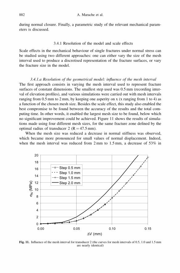
3.4.1.a Resolution of the geometrical model: influence of the mesh interval

The first approach consists in varying the mesh interval used to represent fracture

surfaces of constant dimensions. The smallest step used was 0.5 mm (recording inter-

val of elevation profiles), and various simulations were carried out with mesh intervals

ranging from 0.5 mm to 2 mm, by keeping one asperity on x (x ranging from 1 to 4) as

a function of the chosen mesh size. Besides the scale effect, this study also enabled the

best compromise to be found between the accuracy of the results and the total com-

puting time. In other words, it enabled the largest mesh size to be found, below which

no significant improvement could be achieved. Figure 11 shows the results of simula-

tions made using four different mesh sizes, for the same fracture zone defined by the

optimal radius of transducer 2 (R¼ 47.5 mm).

When the mesh size was reduced a decrease in normal stiffness was observed,

which became more pronounced for small values of normal displacement. Indeed,

when the mesh interval was reduced from 2 mm to 1.5 mm, a decrease of 53% in

Fig. 11. Influence of the mesh interval for transducer 2 (the curves for mesh intervals of 0.5, 1.0 and 1.5 mmare nearly identical)


normal stiffness was determined, for a normal displacement of 0.05 mm. A 9% de-

crease in normal stiffness was observed in the case of a normal displacement of

0.14 mm. Furthermore, there was almost no further change when the mesh size was

reduced below 1.5 mm.

These observations can be explained by studying the proportion of contact area

between both walls. Figure 12 shows the contact zones, for a vertical displacement of

0.1 mm and two different mesh sizes. The location of these contact zones is an output

provided by the model. When the mesh size decreases the contact area also decreases,

but the contacting asperities become more numerous. Because the model takes inter-

action between asperities into account (cf. Section 3.2), a larger number of asperities

leads to a smaller value of normal stiffness. Furthermore, it is known from previous

studies (Marache, 2002) that greater mesh sizes lead to smoother representations of

the fracture surfaces, and thus to thinner void spaces. This tendency leads to an

increase in normal stiffness when the mesh size is increased.

As a result of various comparisons, a mesh size of 1 mm was chosen for all of the

simulations: this size was found to provide the best compromise between computing

time and the accuracy of results. All of the results presented in the following are

derived from simulations using this mesh interval. Another approach which could be

used to study the scale effect would be to vary the fracture size, whilst setting the mesh

interval to a constant value of 1 mm.

3.4.1.b Influence of the fracture size

Variations in fracture size were implemented by increasing the fracture radius, by

5 mm increments, from 5 mm to 45 mm. Figures 13 and 14 show respectively the

fracture closure curves, and the void height distributions, for each value of fracture

radius. To perform these calculations, an isolated fracture was considered for each

Fig. 12. Contact zones for a vertical displacement of 0.1 mm (transducer 2)


radius value, such that the same asperity could be assigned slightly different height

values, depending on the chosen value of fracture radius.

Figure 13 shows that when the radius is increased the normal stiffness (given by the

slope of the curve) decreases for a given normal displacement; Fig. 14 illustrates that the

void height distribution has a smaller range (except for the 5 mm curve) with higher

aperture values. The curve corresponding to a radius of 5 mm is different from the others

Fig. 13. Fracture closure simulations for various fracture radii

Fig. 14. Void height distributions for various fracture radii


because the morphology of this studied zone has been totally interpolated by kriging;

indeed, as we can see on Fig. 4, a hole was present in the fracture for the purpose of

hydraulic tests. The differences between the curves decrease with increasing radius; this

observation emphasizes the well-known problem of the scale effect between laboratory

and in-situ conditions: a fracture too small in size will lead to an overestimation of the

normal stiffness and to an underestimation of the fracture aperture. Nevertheless, it can

be seen in Figs.13 and 14 that the results are very similar for fracture radii greater than

or equal to 30 mm. This threshold value corresponds to the second morphological

structure identified in a prior variographical study (Marache et al., 2002) where an

accurate geostatistical study led to the analysis of roughness correlation structures, in

which two major structures were identified, equal to 15 mm and 30 mm.

In conclusion, the scale effect described above is not caused by the fracture’s

mechanical properties (because these are the same whatever its size), but rather by

its morphological characteristics. In order to gain a better understanding of the causes

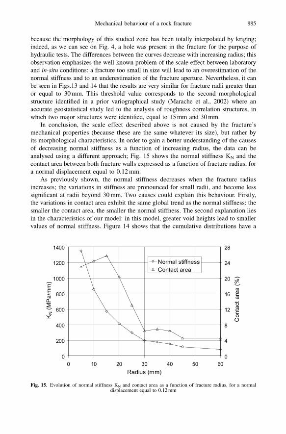
of decreasing normal stiffness as a function of increasing radius, the data can be

analysed using a different approach; Fig. 15 shows the normal stiffness KN and the

contact area between both fracture walls expressed as a function of fracture radius, for

a normal displacement equal to 0.12 mm.

As previously shown, the normal stiffness decreases when the fracture radius

increases; the variations in stiffness are pronounced for small radii, and become less

significant at radii beyond 30 mm. Two causes could explain this behaviour. Firstly,

the variations in contact area exhibit the same global trend as the normal stiffness: the

smaller the contact area, the smaller the normal stiffness. The second explanation lies

in the characteristics of our model: in this model, greater void heights lead to smaller

values of normal stiffness. Figure 14 shows that the cumulative distributions have a

Fig. 15. Evolution of normal stiffness KN and contact area as a function of fracture radius, for a normaldisplacement equal to 0.12 mm


right-hand distribution tail when the fracture radius increases, which could explain the

decrease in stiffness.

Nevertheless, these two curves do not show the same evolution for radii ranging

between 5 mm and 15 mm (decrease in normal stiffness and stabilization of the contact

area). This observation emphasizes the significant role played by interactions between

asperities, which are correctly taken into account in our model (see Section 3.2): for

the same value of contact area, the position of the contact areas on the fracture plays

an important role in the normal stiffness (Hopkins, 1990). In the present case, the

contact areas are considerably more dispersed when the radius is equal to 5 mm than

when it reaches a value of 15 mm.

The spatial location of contact areas thus plays an important role in the mechanical

response of the fracture, and in the determination of possible channels for the flow of

fluids. In the following we present detailed results of the spatial and quantitative

evolution of contact zones during closure of a fracture.

3.4.2 Spatial and quantitative evolution of contact zones as a function

of normal stress

During fracture closure, the total normal stress is distributed over contact areas be-

tween both walls of the fracture. In preparation for future studies of fluid flow through

fractures, it is important to analyze the evolution of these contact areas when the

normal stress increases. Figures 16 and 17 illustrate the evolution of contact areas,

respectively as a function of fracture closure and of applied normal stress.

In Fig. 16, a small increase in contact area can be observed in response to small

levels of fracture closure, followed by a greater rate of change beyond 0.07 mm of

vertical displacement. The latter value corresponds to the initial fracture closure

Fig. 16. Contact area as a function of fracture closure


identified in Section 2.2.1. As opposed to this non-linear response, the contact area

increases linearly as a function of normal stress (Fig. 17), as was previously observed

by Borri-Brunetto et al. (1998). Other authors have shown in various ways that, with

such results, a fast initial increase of contact area is observed in response to normal

stress, followed by a slower rate of change and finally an asymptotic behaviour for

high levels of normal stress (Gentier, 1986; Re and Scavia, 1999; Flamand, 2000). It

should be noticed that in the present case the normal stress levels reached are small

compared to those presented in the papers of many other authors, such that our results

are relevant only to the first part of the normal stress range.

Having quantified the evolution of contact areas during fracture closure, the

spatial distribution of these contacts over the fracture surface can now be studied

for four levels of normal stress (Fig. 18). This figure reveals a very heterogeneous

distribution of contact zones over the fracture, with a very dense zone around sensor

2 for the greatest normal stress values. This result is in total agreement with

the mechanical results and void height distribution presented in Section 2.2, in which

the smallest apertures are located around sensor 2. If the local stress applied in the

contact zones is observed, it is found to reach values significantly greater than the

compressive strength of the material (75 MPa), without damage to the fracture sur-

faces; this result points to the existence of asperity confinement. Furthermore, it is

found that the local stress is higher on isolated asperities than on asperities belonging

to a cluster, because the model takes into account the inter-asperity interaction phe-

nomenon. Finally, when the normal stress increases, the extension of pre-existing

zones is observed (see the surrounded area), rather than the creation of new contact

zones.

The last application of the model involved the study of the influence of variations

in mechanical parameters on fracture closure behaviour.

Fig. 17. Contact area as a function of applied normal stress


3.4.3 Parametric study of mechanical parameters

The developed model allows parametrical studies to be carried out, by varying me-

chanical input parameters (Young’s modulus and Poisson’s ratio). Furthermore, be-

cause the model takes asperities and the bulk material surrounding the asperities into

account, different values can be assigned to the mechanical parameters of asperities

and bulk material. In practice, for geological reasons, the asperities which are in direct

contact with air or fluids can indeed be weakened and have poorer mechanical char-

acteristics than neighbouring portions of intact rock.

3.4.3.a Young’s modulus

The influence of variations in Young’s modulus can be studied by assigning the same

value to asperities and bulk material. Because the model is based on the principle of

superposition in linear elasticity, the normal stiffness for a given value of fracture

Fig. 18. Contact zone localisations for four normal displacement values (the spot size is proportional to theapplied local stress, which ranges from 0 MPa to 933 MPa)


closure is directly proportional to Young’s modulus. As an example, for a normal

displacement of 0.14 mm and a Poisson’s ratio equal to 0.19, the normal stiffness is

equal to 0.0085 times=mm Young’s modulus. This linear relationship implies that the

contact area between both walls corresponding to a constant fracture closure is the

same, whatever the value of Young’s modulus. This can easily be checked, by analys-

ing the spatial distribution of contact surfaces over the fracture after running the

simulation.

Secondly, the value of Young’s modulus can be different for the asperities and for

the bulk material, as previously explained. Figure 19 shows the results obtained for

simulations using three different values of Young’s modulus for the asperities, and a

constant setting for Young’s modulus for the bulk material (30,000 MPa) and Poisson’s

ratio (0.19). The results are presented for the portion of the fracture which corresponds

to the measurement zone of sensor 2.

It can be clearly seen that an increase in Young’s modulus leads to an increase in

normal stiffness. However, this tendency is clearly weaker than in the previous case.

Furthermore, the previously observed linear relationship between both parameters is not

present here; for example, for a vertical displacement equal to 0.14 mm, the results show

a 5% increase in normal stiffness when Young’s modulus varies from 10,000 MPa to

20,000 MPa, as opposed to a 1% change when it varies from 20,000 MPa to 30,000 MPa.

It can thus be concluded that increases in normal stiffness related to changes in

Young’s modulus are due mainly to variations in Young’s modulus of the bulk mate-

rial, and not to that of asperities. This result also confirms the conclusions of Hopkins

(1990) and Capasso (2000), who showed that fracture deformation is mainly due to

deformations of the bulk material, rather than to that of the asperities. This conclusion

becomes even more valid when the largest fracture opening is small (Marache, 2002);

Fig. 19. Influence of variations in Young’s modulus for asperities only (transducer 2, Eintact rock¼30,000 MPa, �¼ 0.19)


in cases where the asperities are relatively high (leading to high aperture values), the

relative contribution of asperity deformations becomes more significant.

3.4.3.b Poisson’s ratio

The last remaining parameter which can be studied in the present context is Poisson’s

ratio. Figure 20 shows fracture closure curves for three values of Poisson’s ratio (the

same value is taken for the asperities and the bulk material); Young’s modulus is set to

30,853 MPa. As in the case of the previous examples, the results presented here

correspond to the portion of the fracture measured by sensor 2.

It can be seen that an increase in Poisson’s ratio leads to a slight increase in normal

stiffness for a given fracture closure, but that the influence of this parameter is

completely insignificant in comparison to that of Young’s modulus.

4. Conclusions and perspectives

A complete understanding of the mechanical behaviour of a fracture under normal

stress is of prime importance in many fields. It was shown at the beginning of this

study that it is not a straightforward task to carry out a normal fracture test under

laboratory conditions, because the choice of transducer location conditions the results:

for a given closure level, the calculated normal stiffness depends on the position of the

transducer. The main parameter influencing the mechanical results is the void height

distribution between both walls of the fracture.

Hopkins’ model (based on a joint deformation model and on the principle of

superposition in linear elasticity) has then been improved by enabling greater fracture

sizes to be modelled and by imposing total-force boundary conditions. Simulations

made with this model have allowed experimental test results to be reproduced, and

Fig. 20. Influence of variations in Poisson’s ratio (transducer 2, E¼ 30,853 MPa)


have provided considerable insight into the extent of the measurement zones relevant

to each transducer.

Various parametric studies have been presented. We have shown that an increase in

fracture size leads to a decrease in normal stiffness, which in our case then stabilizes at

a fracture radius of 30 mm; this threshold value can be explained by morphological

considerations, which are enhanced by a previous geostatistical study (Marache et al.,

2002). With regard to the spatial evolution of contact zones during fracture closure, we

observed an increase of pre-existing zones rather than the creation of new contact

zones. Finally, with regard to the variation of mechanical parameters (Young’s modu-

lus and Poisson’s ratio), we have shown that Young’s modulus for the bulk material

surrounding the asperities is the most influential parameter, and that variations in

Poisson’s ratio have very little impact on normal stiffness.

Various perspectives can be envisioned with regard to the behaviour of fractures.

Firstly, our model should be extended to include the effects of shear behaviour, in

order to forecast peak and residual shear stress as a function of fracture surface

morphology (shearing direction), and under constant normal stress or constant normal

stiffness conditions. The outputs of such a model could be the predicted location of

damaged zones, or the evolution of void space during the shear process; these results

could then be compared with those obtained using other tools (Marache et al., 2003).

Void space evolution during shearing is of prime importance to hydraulic studies.

As an example, such predictions could be used to analyse fluid flow through fractures

for resource recovery problems. Secondly, although fracture surfaces are considered to

be homogeneous with regard to mechanical parameters, the majority of rocks are

polyminerals and their mechanical parameters can vary as a consequence. Because

the model is based on the definition of asperities, we could assign different mechanical

parameter values to each asperity, in order to simulate a polymineral fracture surface.

Finally, the problem of scale effects needs to be addressed by simulating a wide range

of fractures, ranging from laboratory to in-situ scales, in order to gain improved

understanding of in-situ mechanical parameters which can later be used by hydrome-

chanical numerical simulators.

References

Bandis S (1980) Experimental studies of scale effects on shear strength and deformation of rockjoints. Ph.D. Thesis, University of Leeds

Bandis SC, Lumsden AC, Barton NR (1983) Fundamentals of rock joint deformation. Int J RockMech Min Sci Geomech Abstr 20: 249–268

Billaux D, Feuga B (1982) Calcul des perm�eeabilit�ees dans un milieu fissur�ee �aa partir de l’�eetat decontraintes. Programme MECHYD, Rapport du BRGM 82 SGN 816 GEG

Borri-Brunetto M, Carpinteri A, Chiaia B (1998) Lacunarity of the contact domain betweenelastic bodies with rough boundaries. PROBAMAT-21st Century: Probabilities and Materials,pp 45–64

Borri-Brunetto M, Chiaia B, Ciavarella M (2001) Incipient sliding of rough surfaces in contact: amultiscale numerical analysis. Comput Methods Appl Mech Engrg 190: 6053–6073

Brown SR, Scholz CH (1986) Closure of rock joints. J Geoph Res 91(B5): 4939–4948Capasso G (2000) Mechanical and hydraulic behavior of a rock fracture in relation to surface

roughness. Ph.D. Thesis, Turin PolytechnicumCook NGW (1992) Natural joints in rock: mechanical, hydraulic and seismic behaviour and

properties under normal stress. Int J Rock Mech Min Sci Geomech Abstr 29(3): 198–223


Davias F (1997) Mod�eelisation num�eerique d’�eecoulements en massif rocheux fractur�ee – contribu-tion �aa la mod�eelisation du comportement hydrom�eecanique des milieux fractur�ees. Ph.D. Thesis,University of Bordeaux 1

Detournay E (1979) The interaction of deformation and hydraulic conductivity in rock fracture –an experimental and analytical study. Improved stress determination procedures by hydraulicfracturing, Final Report, University of Minnesota, Minneapolis, vol. 2

Flamand R (2000) Validation d’une loi de comportement m�eecanique pour les fractures rocheusesen cisaillement. Ph.D. Thesis, Universit�ee du Qu�eebec �aa Chicoutimi

Gangi AF (1978) Variation of whole and fractured porous rock permeability with confiningpressure. Int J Rock Mech Min Sci Geomech Abstr 15: 249–257

Gentier S (1986) Morphologie et comportement hydrom�eecanique d’une fracture naturelle dans legranite sous contrainte normale – Etude exp�eerimentale et th�eeorique. Ph.D. Thesis, Universit�eed’Orl�eeans

Gentier S, Hopkins DL (1997) Mapping fracture aperture as a function of normal stress using acombination of casting, image analysis and modeling techniques. Int J Rock Mech Min Sci34(3–4): 132.e1–132.e14

Goodman RE (1976) Methods of geological engineering in discontinuous rocks. West, New YorkGreenwood JA, Tripp JH (1971) The contact of two nominally flat rough surfaces. Proc I Mech

Eng 185(48): 625–633Greenwood JA, Williamson JBP (1966) Contact of nominally flat surfaces. Proc Royal Soc

London A (295): 300–319Hertz H (1882) €UUber die Ber€uuhrung fester elastischer K€oorper. J f€uur die Reine Angewandte

Mathematic 92: 156–171Hopkins DL (1990) The effect of surface roughness on joint stiffness, aperture, and acoustic wave

propagation. Ph.D. Thesis of the University of California at Berkeley, Spec. Eng Mater SciMiner Eng

Hopkins DL (2000) The implications of joint deformation in analysing the properties andbehavior of fractured rock masses, underground excavations, and faults. Int J Rock Mech MinSci 37: 175–202

Lanaro F (2001) Geometry, mechanics and transmissivity of rock fractures. Ph.D. Thesis, RoyalInstitute of Technology Stockholm

Lee SD, Harrison JP (2001) Empirical parameters for non-linear fracture stiffness from numericalexperiments of fracture closure. Int J Rock Mech Min Sci 38: 721–727

Marache A (2002) Comportement m�eecanique d’une fracture rocheuse sous contraintes normale ettangentielle. Ph.D. Thesis, Ecole Centrale Paris

Marache A, Riss J, Gentier S, Chil�ees J-P (2002) Characterization and reconstruction of a rockfracture surface by geostatistics. Int J Numer Anal Meth Geomech 26(9): 873–896

Marache A, Riss J, Gentier S (2003) Simulation of the mechanical behavior of a fracture inshear: implication on the distribution of the void space. 10th Int. Congress Rock Mechanics,pp 803–808

Matsuki K, Wang EQ, Sakaguchi K, Okumura K (2001) Time-dependent closure of a fracturewith rough surfaces under constant normal stress. Int J Rock Mech Min Sci 38: 607–619

Pyrak-Nolte LJ, Morris JP (2000) Single fractures under normal stress: the relation betweenfracture specific stiffness and fluid flow. Int J Rock Mech Min Sci 37: 245–262

Re F, Scavia C (1999) Determination of contact areas in rock joints by X-ray computertomography. Int J Rock Mech Min Sci 36: 883–890

Shehata WM (1971) Geohydrology of Mount Vernon Canyon area. Ph.D. Thesis, ColoradoSchool of Mines

Swan G (1983) Determination of stiffness and other joint properties from roughness measure-ments. Rock Mech Rock Engng 16: 19–38

Timoshenko SP, Goodier JN (1970) Theory of elasticity. McGraw-Hill Company, New-YorkTsang YW, Witherspoon PA (1981) Hydromechanical behavior of a deformable rock fracture

subject to normal stress. J Geoph Res 86(B10): 9287–9298Walsh JB (1965) The effect of cracks on the uniaxial elastic compression of rocks. J Geoph Res

70(2): 399–411

892 A. Marache et al.: Mechanical behaviour of a rock fracture

Experimental and modelled mechanical behaviour of a rock fracture under normal stress

Documents

Transcript of Experimental and modelled mechanical behaviour of a rock fracture under normal stress