Exchange of Materials Between TerrestrialEcosystems and the Atmosphere

HAROLD A. MOONEY, PETER M. VITOUSEK, PAMELA A. MATSON

Many biogenic trace gases are increasing in concentrationor flux or botij in the atmosphere as a consequence ofhuman activities. Most of these gases have demonstratedor potmtial effects on atmospheric chemisty, climate,and the functioning of terrestrial ecosystems. Focusedstudies of the interactions between the atmosphere andthe biosphere that regulate trace gases can prove bothour understanding ofterstrial sym and our abili-ty to predict regional- and global-scale canges in atmo-spheric chemisty.

HE STEADILY INCREASING CONTENT OF CARBON DIOXIDEin the atmosphere (1.5 ± 0.2 ppm/year) has provided an

Tunequivocal signal of the global impact of human activities(1). Moreover, a number ofother gases ofbiotic or industrial origin,or both, are increasing in concentration in the troposphere, as wellas having direct and indirect effects on terrestrial biota. The sources,sinks, and dynamics of these trace gases are important for severalreasons. First, many gases affect the chemistry and physics of theatmosphere and thus alter characteristics as diverse as the energybudget of the earth, the concentration of oxidants in the tropo-sphere, and the absorption of ultraviolet radiation in the strato-sphere. Attempts to predict the future evolution of the atmospheremust account for biological processes that regulate these gases.Second, trace gases or their reaction products affect terrestrial biotadirectly in ways that can be more or less species-specific and thatrange from enhancing productivity or competitive ability to causingsubstantial mortality. Finally, the production and consumption oftrace gases in terrestrial ecosystems indicate the presence andmagnitude of particular physiological processes or ecosystem fluxesor both (Fig. 1). Measurement and understanding oftrace gas fluxeswill thus be useful for understanding terrestrial ecosystem dynamicsas well as the atmosphere.

In this article we examine the biotic interactions of trace gases andnote the mechanisms that produce them, their local and regionalpattems of production, and their potential effects on the biota. Wealso discuss how human perturbations modify the extent andpatterns of gascous emissions from, nantral systems. In most casesthere are substantial uncertainties in Qur knowledge of the sources,sinks, or effects of particular gases. Nonetheless, advances in infor-mation, concepts, and techniques place the ability to understand theglobal fluxes and effects of trace gases increasingly within our grasp.

Relatively Stable GasesTrace gases in the atmosphere vary from highly reactive species

with lifetimes in seconds to hours to stable compounds withatmospheric lifetimes of years to centuries. Concentrations of themore stable gases are generally higher (except for the whollyanthropogenic chlorofluorocarbons), their distribution and seasonalpatterns are better characterized, and their increasing concentration,sin the atmosphere are often documented by direct measurementsand by analyses of air bubbles trapped in Antarctic ice (2, 3). Wefirst summarize information on carbon dioxide (CO2), methane(CGE4), and nitrous oxide (N20), thrce relatively stable biogenicgases that are increasing globally. We then discuss biotic sources andinteractions of water vapor and of more reactive trace gases.

Carbon dioxide. The extent, causes, and consequences ofincreasingCO2 concentrations in the atmosphere have been discussed thor-oughly elsewhere (1, 4). The complexities of this analysis have beenformidable. At first, even the sources and sinks of CO2 werecontroversial, although now alternative estimates are increasinglyconvergent. The effect of increasing CO2 on climate has been moredifficult to demonstrate or to predict (5), but overall the mostdifficult problem has been predictng biotic responses to the directeffects of increasing C02 as weU as to indirect effects of a changingclimate.Trtrial rces and sinks of CO2. Ecosystems produce CO2

th.rough respiration. Respiration is positively related to temperaturefor a given organism, but different kinds of organisms differ in theirrate of respiration at a glven temperature. For example, cold climateplants may respire as rapidly at a cold temperature as do warmclimate plants at a higher temperature.

Overall, approximately 100 x iO'5 g of carbon (gC) are releasedinto the atmosphere per year through respiration. Fire is anothersource of C02; it can be considered a form of rapid decompositionsince it quickly releases chemically bound carbon that decomposers

Fig. 1. Exchange of gases between ecosystem components and the atmo-

sphere.

SCIENCE, VOL. 238

H. A. Mooney and P. M. Vitousek are at thc Department of Biological Scicnces,Stanford University, Stanford, CA 94305. P. A. Matson js at the Ecosystem Science andTcchnology Brn*, NASA-Ames Research C e, Molett Field, CA 94035.

9Z6

on

Oct

ober

4, 2

014

ww

w.s

cien

cem

ag.o

rgD

ownl

oade

d fr

om

on

Oct

ober

4, 2

014

ww

w.s

cien

cem

ag.o

rgD

ownl

oade

d fr

om

on

Oct

ober

4, 2

014

ww

w.s

cien

cem

ag.o

rgD

ownl

oade

d fr

om

on

Oct

ober

4, 2

014

ww

w.s

cien

cem

ag.o

rgD

ownl

oade

d fr

om

on

Oct

ober

4, 2

014

ww

w.s

cien

cem

ag.o

rgD

ownl

oade

d fr

om

on

Oct

ober

4, 2

014

ww

w.s

cien

cem

ag.o

rgD

ownl

oade

d fr

om

on

Oct

ober

4, 2

014

ww

w.s

cien

cem

ag.o

rgD

ownl

oade

d fr

om

would otherwise release over a period of time. Estimates of globalCO2 release through biomass burning range from 2 x 10" to5 x 1015 gC year-1 (6, 7); fossil fuel combustion releases 5 x 1015gC year'-. The earth's terrestrial ecosystems also serve as enormoussinks for CO2 and take up through photosynthesis almost the sameamount as is released in respiration and fires.Region variation. The terrestrial ecosystems ofthe earth's surface

vary in their productive capacity and their rates of CO2 exchangeand carbon storage depending on temperature and the availability ofwater and nutrients. For example, nutrient-rich tropical swamps andmarshes have less than a quarter of the areal extent of boreal forestsand yet have a greater total CO2 exchange. Humid tropical forestsconstitute only 6.6% of the earth's terrestrial surface area but haveover 17% of the total net primary production (8).The CO2 released from fires also varies regionally. Moist tropical

forests have estimated mean annual carbon release rates through fireof 30 g m-2 year1, in contrast to 150 g m-2 yearI for seasonallydry tropical savannas and scrubland. Fires in dosed tropical andsubtropical forests contribute 0.5 x 1015 gC year-', whereas tem-perate broadleaf forests contribute only 0.1 x 1015 gC year-';tropical woodlands and savannas contribute the greatest amounts at1.5 x 10i5 gC yeaC' (7).

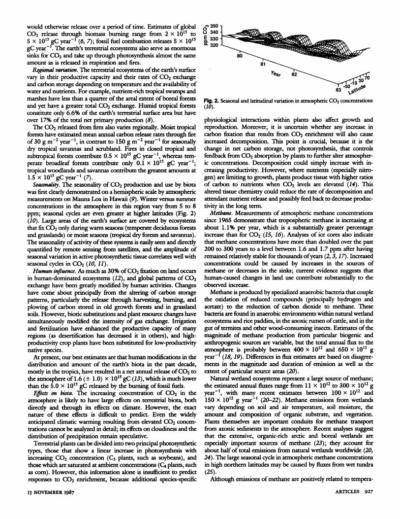
Seasonality. The seasonality of CO2 production and use by biotawas first dearly demonstrated on a hemispheric scale by atmosphericmeasurements on Mauna Loa in Hawaii (9). Winter versus summerconcentratons in the atmosphere in this region vary from 5 to 8ppm; seasonal cycles are even greater at higher latitudes (Fig. 2)(10). Large areas of the earth's surface are covered by ecosystemsthat fix CO2 only during warm seasons (temperate deciduous forestsand grasslands) or moist seasons (tropical dry forests and savannas).The seasonality of activity ofthese systems is easily seen and directlyquantified by remote sensing from satellites, and the amplitude ofseasonal variation in active photosynthetic tissue correlates well withseasonal cycles in CO2 (10, 11).Human influence. As much as 30% ofCO2 fixation on land occurs

in human-dominated ecosystems (12), and global pattems of CO2exchange have been greatly modified by human activities. Changeshave come about principally from the altering of carbon storagepatterns, particularly the release through harvesting, burning, andplowing of carbon stored in old growth forests and in grasslandsoils. However, biotic substitutions and plant resource changes havesimultaneously modified the intensity of gas exchange. Irrigationand fertilization have enhanced the productive capacity of manyregions (as desertification has decreased it in others), and high-productivity crop plants have been substituted for low-productivitynative species.At present, our best estimates are that human modifications in the

distribution and amount of the earth's biota in the past decade,mostly in the tropics, have resulted in a net annual release ofCO2 tothe atmosphere of 1.6 (± 1.0) x 1015 gC (13), which is much lowerthan the 5.0 x 10" gC released by the burning of fossil fuels.

Efects on biota. The increasing concentration of CO2 in theatmosphere is likely to have large effects on terrestrial biota, bothdirectly and through its effects on climate. However, the exactnature of these effects is dffilt to predict. Even the widelyanticipated climatic warming resulting from elevated CO2 concen-trations cannot be analyzed in detail; its effects on cloudiness and thedistribution of precipitation remain speculative.

Terrestrial plants can be divided into two principal photosynthetictypes, those that show a linear increase in photosynthesis withincreasing CO2 concentration (C3 plants, such as soybeans), andthose which are saturated at ambient concentrations (C4 plants, suchas com). However, this information alone is insufficient to predictresponses to CO2 enrichment, because additional species-specific

o 3500 340E 330

(10).

physiological interactions within plants also affect growth andreproduction. Moreover, it is uncertain whether any increase incarbon fixation that results from CO2 enrichment will also causeincreased decomposition. This point is crucial, because it is thechange in net carbon storage, not photosynthesis, that controlsfeedback from C02 absorption by plants to further alter atmospher-ic concentrations. Decomposition could simply increase with in-creasing productivity. However, where nutrients (especially nitro-gen) are limiting to growth, plants produce tissue with higher ratiosof carbon to nutrients when C02 levels are elevated (14). Thisaltered tissue chemistry could reduce the rate of decomposition andattendant nutrient release and possibly feed back to decrease produc-tivity in the long term.Methane. Measurements of atmospheric methane concentrations

since 1965 demonstrate that tropospheric methane is increasing atabout 1.1% per year, which is a substantially greater percentageincrease than for CO2 (15, 16). Analyses of ice cores also indicatethat methane concentrations have more than doubled over the past200 to 300 years to a level between 1.6 and 1.7 ppm after havingremained relatively stable for thousands ofyears (2, 3, 17). Increasedconcentrations could be caused by increases in the sources ofmethane or decreases in the sinks; current evidence suggests thathuman-caused changes in land use contribute substantially to theobserved increase.Methane is produced by specialized anaerobic bacteria that couple

the oxidation of reduced compounds (principally hydrogen andacetate) to the reduction of carbon dioxide to methane. Thesebacteria are found in anaerobic environments within natural wetlandecosystems and rice paddies, in the anoxic rumen ofcattle, and in thegut of termites and other wood-consuming insects. Estimates ofthemagnitude of methane production from particular biogenic andanthropogenic sources are variable, but the total annual flux to theamosphere is probably between 400 x 1012 and 650 x 1012 gyear'1 (18, 19). Differences in flux estimates are based on disagree-ments in the magnitude and duration of emission as well as theextent of particular source areas (20).

Natural wetland ecosystems represent a large source of methane;the estimated annual fluxes range from 11 X 1012 to 300 x 1012 gyear'I, with many recent estimates between 100 x 1012 and150 x 1012 g year'1 (20-22). Methane emissions from wetlandsvary depending on soil and air temperature, soil moisture, theamount and composition of organic substrate, and vegetation.Plants themselves are important conduits for methane transportfrom axonic sediments to the atmosphere. Recent analyses suggestthat the extensive, organic-rich arctic and boreal wetlands areespecially important sources of methane (23); they account forabout half of total emissions from natural wedands worldwide (20,24). The large seasonal cycle in atmospheric methane concentrationsin high noriern latitudes may be caused by fluxes from wet tundra(25).Although emissions ofmethane are positively related to tempera-

13 NOVEMBER 1987 ARTICLES 927

ture over a broad range, freshwater swamps at lower latitudesapparently have lower emission rates than northem peatlands (26),which is possibly caused by differences in organic matter content.Recent measurements in the Amazon floodplain found relativelyhigh emissions in macrophyte beds; Devol et al. (27) estimatedannual emissions of 7.8 x 1012 to 13.2 x 1012 g for the Amazonbasin as a whole. Human activity that alters wetlands (for example,draining or flooding) alters methane emission.

Rice paddies also produce methane, with estimates ranging from35 x 1012 to 170 x 1012 g year-' (28, 29). Most emission datahave been obtained in areas with relatively intensive agriculturalpractices and thus may not represent worldwide rates. The dominantform of transport of methane to the atmosphere appears to bethrough plants. Activities that alter the productivity of rice paddies(for example, continuous inundation or multiple cropping) or

extend their areal extent will increase methane emission. Seiler andConrad (30) estimate that methane emissions may have increasedfrom 75 x 1012 g year-' in 1950 to 115 x 1012 g year-1 in 1980because of increases in the areal extent of rice paddies.

Estimates of methane produced by microorganisms in the numenof cattle, goats, and sheep range from 60 X 1012 to 200 x 1012 gyear-' (21, 22, 31). A recent review (32) calculated production byall animals as a function of animal diet, nutrition, and species; it wasestimated that domestic animals produce 74 x 1012 g year-'.Increased populations of grazing animals have caused a fourfoldincrease in methane production by this source since 1890, andfiuther land-use changes that convert forest to pasture-grazingsystems will lead to further increases in methane production.

Tenrites are an additional natural source of methane. Based on

laboratory studies, Zimmerman et al. (33) estimated that this sourcecontributes 150 x 1012 g year-'. Some subsequent studies (29, 34,35) suggest that methane emissions from termite nests are consider-ably less, perhaps as low as 15 x 1012 g year', but the issue is notfilly resolved. If land dearing from forest to pasture increasestermite populations, this source could become more important.Mining of fossil fuels and emissions from solid-waste disposal sitesalso appear to be relatively important sources of methane (36).

Effects on tral ecasystems. Increased methane in the atmo-

sphere affects terrestrial ecosystems through its effects on climateand atmospheric chemistry. Methane acts as a strong greenhouse-effect gas by absorbing outgoing inftared radiation within thetroposphere 20 times more effectively per molecule than CO2.Moreover, because it is temperature-dependent, methane produc-tion itself may increase with atmospheric warming in the mid- tohigh-northern latitudes. Finally, methane strongly reacts with theatmospheric hydroxyl radical (OH) and can be involved in theproduction of tropospheric carbon monoxide and ozone (03).The direct effects of increased methane concentrations are much

less certain. Dryland soils represent a sink for methane (37, 38), buttheir uptake is small compared to reaction with hydroxyl radical.The extent to which uptake by soils increases with increasedatmospheric concentrations is unknown, as is the effect of anyincreased uptake on populations ofmethane-oxidizing soil microor-ganisms.

Nitrous de. Nitrogen is the most abundant element in theatmosphere, but it is also the element that most limits photosynthe-sis and primary production in most agricultural and many naturalterrestrial ecosystems. This apparent paradox arises because theenormous pool of dinitrogen [3.9 x 1021 g of dinitrogen (N2)] inthe atmosphere can be converted to biologically available forms ofnitrogen by only relatively few species of prokaryotes, and becausebiological nitrogen fixation itself is energetically expensive.

Considerable effort has gone into understanding nitrogen cyclingat scales ranging from local to global (39). Biological nitrogen

fixation in natural ecosystems has been estimated at about 90 x 1012g globally; human-caused nitrogen fixation (by industrial fixationfor fertilizers, by legume crops, and as a by-product of internalcombustion) is about the same magnitude (40). Our currentunderstanding offluxes ofnitrogen gases from terrestrial ecosystemsto the atmosphere is less certain (41). Dinitrogen is the mostabundant form emitted; it is produced by microbiological denitrifi-cation of nitrate. However, dinitrogen is inert and for all practicalpurposes invariant in the atmosphere (atmospheric lifetime is esti-mated at >107 years). Nitrous oxide (N20) is a relatively stable gasthat is present in the annosphere at concentrations around 300ppbv; its concentraions are now increasing at -0.2% per yearglobally (3, 16, 34).

Nitrous oxide is produced as an intermediate in the process ofdenitrification; under some conditions, it can even be the majorproduct (41). Denitrification is most rapid in anaerobic soils with anabundant supply of nitrate and oxidizable carbon, but it can alsooccur in anaerobic microsites within generally aerobic soils (42).Nitrous oxide can also be produced by biomass burning or fossilfuels (43, 44), by nitrifying bacteria (45), and apparently in smallamounts by a wide range of soil microorganisms (46).The major sink for N20 is reaction with activated oxygen in the

stratosphere. Approximately 10 x 1012 g of N20 are consumedannually by this pathway. The eistence or importance ofother sinksis uncertain, although denitifying organisms can use nitrous oxideas a substrate. The annual increase in nitrous oxide concentrations inthe atmosphere amounts to approximately an additional 3 x 1012 g.To balance these sinks, the oceans are a minor source, whereastropical forest soils appear to be a major source (38, 47) and accountfor perhaps as much as 6 x 1012 to 8 x 1012 g year'1. Most tropicalforests circulate much more nitrogen annually than do most temper-ate or boreal forests (48), and even within the tropics, N20 fluxesare significantly larger from nitrogen-rich than nitrogen-poor forests(49). Fertilized agricultural ecosystems also emit more nitrous oxidethan do most natural ecosystems (50, 51). The global increase innitrous oxide concentrations can be explained primarily by combus-tion sources (44); it is uncertain whether the increased use ofnitrogen fertirs in agriculture or increases in deforestation andother land use changes (47, 52) contribute significantly.

Effcts on terrsial ecosystems. Nitrous oxide is a greenhouse gas,and its increasing concentrations are expected to contribute a smallamount towards global warming in the next 50 years (53). Addi-tionally, nitrous oxide oxidizes to nitric oxide in the stratosphere,and stratospheric nitric oxide reacts with ozone there. Increasingconcentrations ofnitrous oxide may thus make a small contributiontoward the breakdown of the stratospheric ozone layer (54),although the wholly anthropogenic chlorofluorocarbons now exerta much greater effect.

The Water CycleWater vapor is a relatively unreactive gas, in that the physical

processes of evaporation and precipitation are quantitatively muchmore important than chemical reactions in controlling its concentra-tions in- the atmosphere; it differs from other unreactive gases in thatits atmospheric lifetime is short (--10 days). Vast quantities ofwatervapor move from the earth's surface through evaporation into theatmosphere and then back again through precipitation annually.The amount involved in this cycle is estimated at 973 mm per yearaveraged over the earths surface, for a total evaporated volume ofabout 500,000 km3 (500 x 1018 g of water) (55).Most ofthe eart's water is stored in the oceans (97.4%) or polar

ice (2%). Here we focus on the less than 1% ofthe water contained

SCIENCE, VOL. 238

in the atmosphere, soil, lakes, and rivers. The atmosphere containsonly 0.001% of the earth's water (13,000 km3 or 13 x 1018 g H20versus 720 x 10'5 gC), which would amount to an average depthover the earth's surface of 20 to 30 mm. There is great spatial andtemporal variation in atmospheric water content, from 50mm in theatmosphere ofsome tropical regions to as low as 5 and 1.5 mm overarctic and antarctic regions, respectively (56). Despite these smallquantities, water vapor is the prime controller of tropospherictemperature structure through its effects on both solar and terrestrialradiation.

Vegetation interacts with the hydrological cyde both directly andindirectly. First, it influences the amount of precipitation that entersthe soil. Some of the incoming precipitation is intercepted byvegetation and evaporates before reaching the ground, the amountof which depends both on the nature of the vegetation and oncharacteristics of precipitation. Annually as much as a third of theincoming precipitation may be intercepted by a wide variety offorest communities ranging from tropical to boreal types (57).Second, vegetation influences the amount of water that enters thesoil profile; vegetation-free surfaces have much greater runoff anderosion rates than vegetated areas (58). Third, the presence ofvegetation alters the amount of intercepted radiation (59), bound-ary-layer characteristics, and the amount of water available forevaporation. Water in the soil below a depth of about 10 to 20 mm(60) is not subject to evaporation unless an area is vegetated, but thepenetrating roots of plants transport water from deep in the soilprofile and bring it to leaf surfaces. There it is in direct contact withthe atmosphere whenever leaf stomatal pores are open (which theygenerally are dunng the day, as long as there is a supply of soilmoisture and the atmosphere is not unusually dry).The influence of vegetation on the hydrological cycle has been

most clearly demonstrated where all of the vegetation on a water-shed has been removed. Streamflow in such watersheds generallyincreases in direct proportion to the amount ofvegetation removed;the recovery period is approximately related to the logarithm oftimesubsequent to felling (61).

Influences ofvegetation type on the hydrological cycle have beenexperimentally demonstrated for evergreen conifers versus decidu-ous hardwoods. Water loss to the atmosphere is greater for pinesthan hardwoods, which is caused in part by the greater leaf andbranch surface area per unit ofground surface ofpines and in part bytheir year-round maintenance of leaves (62). Even species-specificeffects have been documented. For example, biological invasions ofsalt-cedar (Tamarix spp.), which are exotic species with unusuallydeep roots, significantly increase evapotranspiration from semiaridregions of the southwestern United States (63).

Regional effects. Almost 70% of the total evaporation on land aswell as over water takes place within the tropical latitudes of30°N to300S, although the fractions of land and water within the tropicsconstitute only 44 and 52%, respectively, of the total global surfaceareas (55). The water balance of different regions also variesconsiderably. Of the 2000 mm of total incoming annual precipita-tion in the Amazon Basin, 48.5% is returned to the atmospherethrough transpiration by the vegetation, 25.6% is returned byevaporation from intercepted water, and about 26% is lost throughrunoff (64). In contrast to the 1500 mm annual evapotranspirationover tropical forests in general, annual water loss over borealconiferous forests is only 240 mm per year. The total evapotranspor-tation from tundra and boreal forest accounts for only 0.7% of theglobal evapotranspiration, although these areas cover 8% of theearth's land area (65).Effts f vegetatn on water bakce and dimate. Because of the

necessity of integrating over large areas, most analyses ofthe effectsof vegetation on regional atmospheric composition and dynamics

13 NOVEMBER I987

are based on simulations that use global circulation models. Mintz(66) reviewed the many simulations in which surface albedo or soilmoisture or both were altered, and noted that whenever soilmoisture or albedo was changed regionally, so was precipitation,temperature, and the movement of the atmosphere. These simula-tions are important and suggestive, but the global circulationmodels in use have very limited land surface inputs. For example, therate of evapotranspiration used for these models is that for openpans rather than for vegetated surfaces. The simulations often useunrealistic inputs, such as a total lack of soil moisture or vegetationover large regions. Models with finer levels of resolution are beingdeveloped and include biophysical models that fully account for theinfluence of vegetation on the transfer of radiation, moisture, andmomentum (67). In these models the properties of the vegetationdetermine land surface interactions with the atmosphere and thusprovide for atmosphere-biosphere interactions. Additionally, mea-surements of stable isotope ratios in precipitation and the atmo-sphere (64) can be used to integrate rates of evapotranspiration overlarge areas and to validate models of evaporation and water trans-port.The further development of techniques for estimating the water

balance is crucial to our ability to predict atmosphere-biosphereinteractions. The amount and distribution of water vapor controlboth atmospheric and ecosystem dynamics directly, and enormousregional changes in water budgets are forecast as the eart's energybalance is altered by the increasing concentrations ofcarbon dioxide,methane, nitrous oxide, and other greenhouse gases.

Reactive GasesA large number of highly reactive gases are produced biologically

or by biomass combustion, and the concentrations ofmany ofthesegases are currently increasing in the atmosphere. These reactivegases pose a very different problem from more stable gases; theirconcentrations are generally low and often ephemeral, so it is moredifficult to identify their sources, sinks, and effects with certainty.Moreover, many of these gases interact in ways that cause theproduction or destruction ofother gases. Globally averaged concen-trations or atmospheric lifetimes of the reactive gases are thus notonly difficult to obtain but also not very informative, because theoccasional coincidence of high concentrations oftwo or more gasesregionally or locally can have a great effect on atmospheric chemistryas well as the terrestrial biota.

Carbon. The major reactive carbon gases are a suite of hydrocar-bons (non-methane hydrocarbons or NMHC) and carbon monox-ide (CO). These two are linked in that oxidation of NMHC is amajor source of atmospheric CO.Non-methane hydnarbons. Two major biogenic dasses ofNMHC

are isoprene (C5H8) and terpenes. Zimmerman et al. (68) estimatedannual global emission rates of 350 x 1012 g and 480 x 1012 g forisoprene and terpenes, respectively, and calculated that the oxidationof these hydrocarbons could account for 39% of global COproduction. Similarly, Logan et al. (69) suggested that biogenichydrocarbons contribute significantly to the production of atmo-spheric CO.Terpene production by plants has been studied for many years in

relation to resistance to and attraction of insects (70), and emissionsof volatile terpenes were first suggested to affect atmosphericchemistry by Went (71). Terpene emissions from vegetation arecontrolled by the chemical potential gradient between leaf andsurrounding air (72, 73), a gradient that is controlled by the vaporpressure of the individual monoterpenes.

Isoprene is also produced and emitted by many plant species (74,

ARTICLES 929

75). Its biosynthesis is associated with photorespiration and inter-mediates of the glycolate pathway (76), and thus its emission isclosely related to light levels and biosynthetic rates. Like terpenes,isoprene emissions increase exponentially with temperature, butthey are more strongly stimulated by light (73, 77).A number of studies have measured isoprene and terpene emis-

sions from individual species and in the atmosphere above vegeta-tion canopies. From these studies, Zimmerman (75) concluded thatthe highest emissions (especially of terpenes) in the United Statesoccur in the northern tier of states, which includes temperatedeciduous and coniferous forest regions. More recent studies ofemissions in tropical areas suggest that rates ofproduction (especial-ly of isoprene) are higher than in cool temperate species (78), andGregory et al. (79) reported elevated concentrations of isoprene inthe planetary boundary layer over forests in Guyana. Greenberg andZimmerman (80) suggested that the Amazon may be a globallyimportant source of biogenic hydrocarbons; ambient levels ofisoprene are similar to northern coniferous forests, but its averageatmospheric lifetime is shorter in the tropics.

Global estimates of isoprene and terpene emission have beenbased on the assumption of a constant relation between foliarbiomass and emission rate for dasses of vegetation. Given thisassumption, permanent conversion of forest to pasture or agricul-ture use would reduce biogenic NMHC emission (but perhapsincrease anthropogenic hydrocarbon emissions through biomassburning and subsequent human activities). However, little informa-tion is available on relations between soil fertility and NMHCemissions or on emissions from successional vegetation; the speciesplanted in short-rotation tree plantations are often prodigioussources ofNMHC (81).

Because of their high reactivity and short atmospheric lifetimes,biogenic NMHC do not directly affect climate. They do interactwith other atmospheric compounds, however, in that their reactionwith ozone can be a significant sink for ozone and a source forcarbon monoxide. Although emissions of terpene and isoprenerepresent a loss offixed carbon to plants on the order of0.5 to 1% ofphotosynthetic uptakes, there is no evidence that atmosphericconcentrations directly affect physiological or biochemical character-istics of vegetation.Carbon monacide. Carbon monoxide is a relatively short-lived gas

(with an atmospheric lifetime ofless than half a year) that appears tobe increasing in the troposphere (19). About 1000 x 1012 g ofcarbon enters the atmosphere annually as CO, about half of whichresults from oxidation ofmethane and NMHC. Fossil fuel combus-tion, agricultural burning, and land-clearing fires account for mostof the remainder (43, 69).Approximately 10% of the CO that is destroyed annually is

consumed in soils; most of the remainder is oxidized by OHradicals. No direct biological effects of current atmospheric levels ofCO are known, but it interacts with nitrogen oxides and OH toproduce tropospheric ozone, which clearly does affect organisms, asdiscussed below.

Nitrogen. The major reactive nitrogen gases are oxides of nitro-gen, collectively referred to as NO.. Combustion is a major sourceof NO.; it is both oxidized from fuel nitrogen and fixed fromatmospheric N2 during combustion (44). Lightning also fixes NO,(82), and NO in particular is produced by the abiotic reduction ofnitrite in acid soils and by biological processes related to nitrificationand denitrification (83). The limited and rather difficult measure-ments of NO. fluxes from soils show that they generally correlatewith N20 fluxes on an annual basis (51), although NO fluxes arerelatively greater when the soil surface is dry. Thus seasonal tropicalforests and ferdlized agriculture probably represent significantsources of NO,.930

NO. plays a complex role in atmospheric chemistry. At lowconcentrations (as in the stratosphere), it catalyzes the breakdown ofozone. At higher concentrations (which are often realized in indus-trially affected air), however, it can interact with CO, OH, andhydrocarbons to produce ozone (84). Moreover, atmospheric NO,is converted within days (more rapidly in solution) to nitric acid thatrepresents a substantial contribution (30 to 50%) to the acidity ofprecipitation within and downwind of industrial regions. Increaseddeposition of fixed nitrogen fertilizes natural and managed ecosys-tems and alters pathways of nitrogen cycling in apparently naturalforests (85). Although this probably increases terrestrial productivi-ty at moderate levels ofdeposition, high levels ofnitrogen depositedinto normally nitrogen-deficient forest ecosystems could causeincreased herbivory (86), undesirable patterns of root-shoot alloca-tion (87), growth limitation by other nutrients, and possiblyincreased mortality (88).

In the longer term, increased nitrogen-deposition is likely to alterdecomposition as well as production by increasing the nitrogencontent and carbon quality of plant litter (89). Moreover, increasednitrogen will probably affect the outcome of competition amongplant species (90), and alter population and community dynamics ineven the best protected nature reserves. The large amounts ofnitrogen deposited on natural and managed ecosystems of northernEurope and eastern North America probably cause many of theseeffects now.Ammonia. Ammonia is also present at low and variable concentra-

tions in the atmosphere, and our knowledge ofammonia fluxes hasbeen limited by analytical difficulties. Ammonia is inpH-dependentequilibrium with nonvolatile ammonium in soils and solutions; itsmajor natural sources appear to be volatilization from alkaline soils,animal excreta, and senescing leaves (91). These sources are proba-bly increased by intensive agriculture and animal husbandry prac-tices.Once in the atmosphere, ammonia can be dissolved or adsorbed

by aerosols and water droplets or taken up directly by vegetation.Most of the ammonia that enters the free troposphere is returned asammonium in bulk precipitation or captured aerosols. Ammonia inaerosols or dissolved in cloud droplets can accept a proton to formammonium, thereby reducing the acid intensity of precipitation.However, where deposited ammonium is retained within terrestrialbiota or lost as nitrate (true of most sites), it can contributesubstantially to soil acidification (92).Ammonia can contribute significantly to the overall deposition of

nitrogen downwind of seabird rookeries (93), feedlots, and agricul-tural regions where anhydrous ammonia or urea are used heavily. Insuch areas it causes effects on nitrogen cycling identical to those ofnitrate derived from NOR.

Sulfur. An even wider variety of trace sulfur gases than nitrogengases are emitted from natural terrestrial ecosystems, and most arerelatively reactive. The most important are hydrogen sulfide (H2S),dimethyl sulfide (DMS), methyl mercaptan (CH3SH), carbon disul-fide (CS2), and carbonyl sulfide (COS); all except COS are short-lived. These gases are produced by a variety of pathways in soils andwithin higher organisms (94, 95); estimates of their fluxes have beenlimited by sparse sampling and insufficiently validated analyticalprocedures, so that these gases will be discussed only briefly.Most of the trace sulfur gases are produced most rapidly in wholly

anaerobic environments, and hence marshes and other wetlandshave been considered relatively active sources of sulfir gas emis-sions. In upland sites, current evidence suggests that at least the fluxof H2S is much greater in tropical than temperate forests (96).However, our knowledge of sulfur gas fluxes remains in a state offlux itself; successive refinements in technique, sampling area, orsampling frequency often alter flux estimates substantially (95).

SCIENCE, VOL. 238

Table 1. The regions and land uses for which emissions of the listed trace gases are believed to be at a maximum. Annual flux is to the atmosphere.

Approximate AtmnosphericNatural system or geographic area m f ASpecies Landuscformaximumflux annualflux (days)of maximnum flux ana lxlftm(log g) (days)CO2 Wet tropical forest Forest, biomass burming 17 -2500H20 Wet tropical forest Forest 20.5 10CH4 Wetlands Rice paddies, pasture (animal 14.5 -3600

husbandry), biomass burningN20 (Fertile) tropical forest Fertilized agriculture, biomass buring 13 -60,000C5H8 Tropicgal forest Forest 14.5 <1CloH16 Temperate forest, shrublands Forest 14.5 <1CO Produced from CXH, in atmosphere Biomass burning 15 75NOX Tropical forest Fertilized agriculture, biomass burning 14 4NH3 Temperate grasslands Pasture (animal husbandry), fenrlized 14 9

agriculture, biomass buringCOS Wetlands Biomass burning 12.5 -900Sulfur gases* Wetlands, wet tropical forest, oceans Ferdlized agriculture, biomass buring 13 2

nudes othe reduced sulfur gases such as hydrogen sulfide (H2S), dMnethYl SUlfide (DMS), mnIe taC and carbon disulfide (CS2).

In addition to biogenic sulfur gases, sulfur ent¢rs the atmosphereas aerosols from sea salt, gas from volcanoes, through deflation ofsulfate-containing dust in arid regions, and as 4 result of biomassand fossil fuel combustion. Fossil fuel combustion is the majorperturbation to the global sulfur cyde, but human acivities can alsochange fluxes of sufur to the atmosphere through the formation ordrainage of wetlands and through desertification.

Effects of additional atmospheric sulfur on terrestrial ecosystemsindude well-documented biotic changes attendant upon lake andstreacidification (97), and alterations ip nutrient cyding withinforest ecosystems (85). Another major effct of splfur s emissionscould be an increase in the background (at times of low volanicactvity) stratospheric sulfate aerosol layer caused by increasingconcentrations (not yet documented) of the relatively stable gasCOS (98).Interaiom with trpspherc ozone. Ozone is unique in that it

absorbs short-wave ultraviolet in the stratospherc and thereby servesto protect living organisms, whereas in the troposphere it is a strongoxidant that can damage organisms (54). Hence both its breakdownin the stratosphere and its increasing concentratons in the tropo-sphere represent serious environmental problems (19). Occasionalepisodes of elevated ozone concentrations are currenty observed inindustrial and developed agicultural regions, and troposphericozone is demonstrably reducing productivity and yield in agriculture(99) and most likely in natural ecosystems in much ofthe developedworld.Many of the reactive gases interact with ozone (and its daughter

product the hydroxyl radical) in complex ways. Hydroxyl radical andozone are major oxidants in the breakdown of CO, CH4, isoprene,and terpenes. At low concentrations of NO, CO oxidation repre-sents a sink for O3. At elevated NO concentrations, however, 03concentrations can actually be increased during GO oxidation (84).This interaction may bc partially responsible for increasing tropo-spheric ozore concentrations in developed regions (100). Furtherincreases in NO concentrations due to fossil fuel combustion,biomass burning, or agricultural fields could cause more widespreadincreases in tropospheric ozone.

ConclusionsThe interactve nature of the biota and the atmnosphere has

become increasingly understood in recent years. Large amounts ofmany biologically produced trace gases are exchange4 annuallybetween the atmosphere and biosphere (Table 1), and many oftheseare now increasing in flux or conce on or both as a consquence

13 NOVIIMBER 1987

of human activities. Although trace gases are often considered interms of globally averaged fluxes, many are highly variable in spaceand time. Tropical forests and wetlands are particularly activesources (Table 1); and these systems are further subject to rapidalteration through land deanng and drainage. uIuman activities thatgenerate trace gases are also concentrated into particular ecosys-tems-fossil fuel combustion is concentrated into the north temper-ate zone, and bionass burning is most active in areas formerlycovered by dry tropical forest and savanna (which are now mostlyagricultural and pasture land).An understanding of atmosphere-biosphere interactions and their

effects is a problem vast in scope, one that encompasses the entireplanetar ecosystem. Unfortunately, the information available is stillinsufficient to -make reasonable projecions on the effects ofchangesthat now occur. What is needed? First, the considerable uncertaintythat surrounds estimates of the various gas fluxes ketween the landand the atmosphere must be reduced. This will nvolve a moreadequate network for global environmental measurements, onewhich emphasizes the control of spatial and temporal variation aswell as new ways for accurately determining land use changes andassociated changes in gas fluxes. Second, methods for measuring andintegrating gas fluxes on regional scales comparable to those used inglobal circulation models must be developed and refined. Finally,experiments must be performed at the level ofwhole ecosystems todevelop the capacity to predict the consequences of a changingatmosphere and climate.New research initiatives are under way that propose such global

studies (101). These initiatves build upon the emerging technologyof laser-based measprements of atmospheric chemistry, planetaryboundary-layer sampling, and means for viewing continuously notonly the state of the earth's terrestrial ecosystems but also of theirexchange processes. A concerted effort in this area should yield theability to analyze and predict how biologically driven fluxes of tracegases either cause or could cause changes in autospheric chemistry,radiation budget and climate, and the functioning pf terrestrialecosystems.

REFERENCES AND NOTES1. J. R. Trabalka, Ed.,AxospheoiCarbDionidc and the GlobalCo Cydce (U.S.

Deparment of Energ, Washington, DC, 1985).2. R. A. -Rasmussen and M. A. K. Khalil,J. Geop*ys. Ret. 89, 11599 (1984); B.

Stauffer, G. Fischr, A. Neftel, H. Ocschger, Scence 229, 1386 (1985).3. G. I. Pearman, D. Ethendge, F. de Silva, P. J. Fraser, Natue (Lodon) .320, 248

(1986).4. B. Bolin, E. T. Degens, S. Kempe, S. Kctner, Eds., The Global Carbon Cyle

(Wiley, New York, 1979); W. Clark, Ed., Cabon Dimide Repie* (Oxford Univ.Press, New York, 1982); E. R. Lemon, Ed., CO2 and Pla (AAAS, Washing-ton, DC, 1983); B. R Strain and J. D. Cure, Eds., E fs fIncreaing

ARTICLES 93I

Carbon Dicde on Vegetation (U.S. Department of Energy, Washington, DC,1985).

5. B. Bolin,, B. R. D66s, J. Jager, R. A. Warrick, Eds., The Greenhouse Efct,Climaw Change, and coystems (Wiley, Chichester, 1986).

6. W. Seiler and P. J. CruMen, Chin. Change 2, 207 (1980).7. J. S. Olson, in Fire Regims andEcsystem Properties, General TcrbniAl Report WO-

26, H. A. Mooney at al., Eds. (U.S. Department of Agriculture, Forcst Service,Washington, DC, 1981), pp. 327-378.

8. G. L. Aijay, P. Kctner, P. Duvigneaud, in The Global Carbon Cydce, B. Bolin, E. T.Degens, S. Kempe, P. Ketner, Eds. (Wiley, New York, 1979), pp. 129-182.

9. R. B. Bacastow and C. D. Keeling, in Carbon Cyle AModeing, B. Bolin, Ed.(Wilcy, New York, 1981), pp. 103-112.

10. C. J. Tucker a al., Nature (London) 319, 195 (1986).11. I. Y. Fung, C. J. Tucker, K. C. Prentice,J. Geoph. Res. 92, 2999 (1987).12. P. M. Vitousek, P. R. Ehrlich, A. H. Ehrlich, P. A. Matson, Biosie 36, 368

(1986).13. R. A. Houghton tal., inAtmospebrc CarbonDiavide and the Global Cw-bon Cycle,

J. R. Trabalka, Ed. (U.S. Department of Energy, Washington, DC, 1985), pp.114-140.

14. W. E. Williams, K. Garbutt, F. A. Bazzaz, P. M. Vitouek, Qecoia 69, 454(1986).

15. D. R. Blake and F. S. Rowland,J. Atmos. Chem. 4, 43 (1986).16. R. A. Rasmussen and M. A. K. Khalil, Am. Geophy. UnionAbsr. (May 1986).17. H. Crai and C. C. Chou, Gophys. Res. Le=t. 9, 1221 (1982).18. Y. Makide and F. S. Rowland, Proc. NatI. Acad. Sci. U.SA. 78, 5933 (1981); E.

W. Mayer at a., ibid. 79, 1366 (1982); F. S. Rowland, Orsins Lsfr 15, 279(1985).

19. Atmosheric Ozone, Glbal Ozown Research and Monxitorin (World MeteorologicalOrganization, Gencva, 1986), voL 1, pp. 57-115.

20. E. Matthews and I. Fung, Global Biogeocem. Cydes 1, 61 (1987).21. M A. K. Khahl and R. A. Rasmussen,J. Gephy. Res. 88, 5131 (1983).22. W. Sedier, in Cur.entPeapeai inMicrobalEcolgy, M. J. Klug.and C. A. Reddy,

Eds. (Ameican Soicty for Microbiology, Washington, DC, 1984) pp. 468-477.23. R. C. Harniss at al., Natum (London) 315, 652 (1985).24. D Se cher et al.,.Tdhs, in press.25. L. P. Steelc at al.,J. Atmos. Chem. 5, 125 (1987).26. R. C. Haffiss and D. I. Scbacher, Geopys. Res. Lett. 8, 1002 (1981).27. A. k. Dcvo$et al. J. Gepys. Res., in prcss.28: R. J. Ci"ceone and J. D. Shettr, ibid. 86, 7203 (1981); A. Holzapfcl-Pschom

And W. Seiler, ibi?. 91, 11803 (1986).29. W. Seiler, A. Holzapfel-Pschorn, R. Conrad, D. Schanffe,J.Atmos. Chem. 1, 241

(1984).'30. W. Seiler and.R. Conrad, The Geophysioljy ofAman (Wiley, New York,

1987).31. D. H. Ehhalt, Tdels 26, 58 (1974); and U. Schmidt, PureAppI. Geophy.

116, 452 (1978).32. P. J. Crutzen, I. Aselmann, W. Sciler, Tellus 38B, 271 (1986).33. P. R. Zimmerman, J. P. Greenberg, S. O. Wandiga, P. J. Crutzen, Scien"c 218,

563 (1982).34. R. A. Rasmussen and M. A. Khalil, Natue (London) 301, 700 (1983).35. N. M. Collins and T. G. Wood, Scence 224, 84 (1984).36. H. G. Bingemer and P. J. Crutzen,J. Geophys. Res. 92, 2189 (1987).37. B C. Harriss, D; I. Sebacher, F. P. Day, Jr., Natur (London) 297, 673 (1982).38. M. Keller at al., Geob. Res. Lett. 10, 1156 (1983).39. F. E. Clark and T. H. Rosswall, Eds., Teretrid Nitren Cyces (Ecological

Bulletin 33, Stockholm, 1981); T. H. Rosswall, Some Persecie of the MajorBiogeochemical Cyces, G. E. Likens, Ed. (Wily, Chichester, 1981), pp. 25-49; G.P. Robemon and T. H. Rosswall, Ecol. Monor. 56, 43 (1986).

40. T. H. Rosswall, The Major Biogeohmical Cyces and Their Interacion, B. Bolinand R. B. Cook, Eds. (Wiley, Chichester, 1983), pp. 46-50.

41. W. B. Bowden, Biogeohmaity 2, 249 (1986).42. A. J. Sexstone t al., Sodi Sci. Soc. Am. J. 49, 645 (1985).43. P. J. Cruizen t al.,J. Atmo. Chem. 2, 233 (1985).44. W. M. Hao, S. C. Wofsy, M. B. McElroy, J. M. Beer, M. A. Toquan,J. Gep*.

Res. 92, 3098 (1987).45. J. M. Bremner and A. M. Blaclkner, Science 199, 295 (1978).46. B. H. Bleakly and J. M. T-iedje, Appl. Environ. Micbil. 44, 1342 (1982).47. M. Keller, W. A. Kaplan, S. C. Wofsy,J. Gephys. Res. 91, 11791 (1986).48. P. M. Vitousek and R. L. Sanford, Jr.,Annu. Rev. Ecol. Syst. 17, 137 (1986).49. P. A. Matson and P. M. Vitousek, Global Biogeocb. Cydes, in press.50. L. L. Goodroad and D. B Keeney,J. Environ. Qual. 13, 448 (1984).51. I. C. Anderson and J. S.. Levinc,J. Gephy. Res. 92, 965 (1987).52. W. B. Bowden and F. H. Bormann, Scen 233, 867 (1986).53. V. Ramanthan at al.,J. Geophys. Res. 90, 5547 (1985).54. R. J. Cicerone, Scence 237, 35 (1987).55. H. Baumgartner and E. Rachel, The Word Water Balan: AManAnnual Glbal

Coninental andMaritim Preciation, Evporation and Runof(Elsevier, Amster-dam, 1975).

56. Inadvrtent Climate Modifications (Massachusets Institute of Technology, Cam-bridge, 1971).

57. J. G. Lockwood, World Climatic Systemu (Arnold, London, 1985).58. R. 0 Meeuwig and P. E. Packer, in Waterced Managcecnt on Range and Foret

Lands, H. F. Heady, D. H. Falkenbourg, J. P. Riey, Eds. (Utah Water RearchLaboratory, Logan, UT, 1976), pp. 105-116.

59. T. R. Oke, Bowunary Layer Clmates (Wily, New York, 1978).60. R E. Sosebee, in WatenhedM nement on Range and ForestLands (Utah Water

Research Laboratory, Logan, UT, 1976), p. 95.61. H. C. Pereira, Land Use and Water Resorc in Temperate and Tropical Climacs

(Cambridge Univ. Press, Cambridge, 1973).62. W. T. Swank and J. E. Douglass, Scenc 185, 857 (1974).63. W. M. Neill, Edncationa Buletin 83.4 (Desert Protective Council, Spring Valley,

CA, 1983).64. E. Salati and P. B. Vose, Scienc 225, 129 (1984).65. P. C. Miller, Variaons in the Global Water Budget (Reidel, Dordrecht, the

Netherlands, 1983), p. 185.66. Y. Mintz, The Global Clmate (Bracknell, United Kingdom, 1984), p. 79.67. P. J. Sellers et al.,J. Atmos. Sc. 43, 505 (1986).68. P. R. Zi n t al., Gphs. Res Let. 5,679 (1978).69. J. A. Logan at al.,J. Geph. Re. 83, 7210 (1981).70. R. W. Stark, Annu. Rep. Entomd. 10, 303 (1964).71. F. W. Went, Natu (Londm ) 187, 641 (1960).72. D. T. Tingey, M. Manning, L. C. Grothaus, W. F. Burns, P)siol. Plant. 47,112

(1979); R. C. Evans, D. T. Tingey, M. L. Gumpcrtz, For. Sa. 31, 132 (1985).73. D. T. Tingey, M. Manning, L. C. Grothaus, W. F. Burns, Plant Physiol. 65, 797

(1980).74. R A. Rasmussen, Environ. Scaw Tech. 4, 667 (1970); P. B ZimmrmnR, U.S.

Environ. Prot. Ageny Rep. 904/9-77-028 (1979); R. C. Evans, D. T. Tingey, M.L. Gumpertz, W. F. Burns, Bot. Gaz. 143, 304 (1982).

75. P. R. Zimmeran, U.S. Environ. Prot. Agency Rep. 450/4-79-004 (1979).76. C. A. Jones and R. A. Rasmussen, PlantPl.sio. 55, 982 (1975); W. D. Loomis

and R. Crotecau, Biochem. Plant 4, 363 (1980); D. T. Tingey, R. Evans, M.Gumpetz, Plana 152, 565 (1981).

77. R. A. Rasmussen And C. A. Jones, Phytochemisty 12, 15 (1973).78. D. R. Cronn and W. Nutmagul, TelUs 34, 159 (1982).79. G. L. Gregory at al., J. Geopys. Res. 91, 8603 (1986).80. J. P. Greenberg and P. R. Zimmerman, ibid. 89, 4767 (1984).81. B. Bolin e al., in The MajorBiogeochemial Cycles and Their Interaions, B. Bolin

and R. B. Cook, Eds. (Wiley, Chichester, 1983), pp. 8-40.82. J. S. Lcvine, T. R. Auguson, I. C. Anderson, J. M. Hoell, D. A. Brewer,Amos.

Envirn. 18, 1797 (1984).83. J. A. Logan,J. Geophys. Res. 88, 10785 (1983).84. P. J. Crutzen, in The Major Biogeocemical Cydes and Their Intmeaio, B. Bolin

and R. B. Cook, Eds. (Wiley, Chichester, 1983), pp. 65-113.85. D. W. Johnson, J. Turner, J. M. Kely, WaterReo. Res. 18, 449 (1982).86. W. J. Mattson, Annu. Rev. Ecld. Syst. 11, 119 (1980).87. R. H. Waring, For. Ecol. Manage. 12; 93 (1985).88. B. Nighlgad,Ambio 14 (No. 1), 2 (1985).89. P. M. Vitouseck,Am. Nat. 119, 553 (1982); J. M. Melillo and J. R. Gosz, in The

MAjor BWeochemial Cycles and Ther Inteacin, B. Bohin and R. B. Cook, Eds.(Wiley, Chichester, 1983), pp. 177-221.

90. D. Tilm, Ecoag 67, 555 (1986).91. G. D. Farquhar at al., in Gaseou Los ofNitnenfivm Plant So Systems, J. R.

Freney and J. R. Simpsn, Eds. (NijhofffJunk, The Hague, 1983), pp. 159-194;D. S. Schiml etal., Bgomisty 2, 39 (1986).

92. D. Bikey and D. Richter, Ad. Ecol. Res. 16, 1 (1987).93. H. Mizutani, H. Hasegawa, E. Wada, Biogeochemesty 2, 221 (1986).94. D. Moller,Atom. Environ. 18, 29 (1984); M. 0. Andreae, in The Biogchemial

Cyces ofSulfur andNinmen in the RemoteAmosphere, J. N. Galloway t al., Eds.(Reidel, Hingham, MA, 1985), pp. 5-25.

95. P. A. Steudler and B. J. Pcteson, Atxm. Envitn. 19, 1411 (1985).96. D. F. Adarm et a., Environ. Sci. Tecnd. 15,1493 (1981); R. Delmas t al.,J.

Geohbs. Res. 85, 4468 (1980).97. J. H. Gibson, Acid Deposition: Long-Tefm Trends (National Academy Press,

Wahington, DC, 1986).98. M. A. K. Khali and R. A. Rasnussen, Atnos. Envion. 18, 1805 (1984).99. W. W. Heck etal., Envimo. Sci. Technol. 17, 573A (1983); P. B. Reich and B. G.

Amundson, Sacenc 230, 566 (1985); S. C. Liu et al.,J. Geophy. Res. 92, 4191(1987).

100. J. A. Logan,J. Geophys. Res. 90, 10463 (1985).101. Earth System Science (National Aeonautics and Spacc Administration, Washing-

ton, DC, 1986), p. 48; Glkbal ChanWe in the Gemphere-Biospere (NationalAcademy Press, Washington, DC, 1986), p. 91; Globil Trpspheric Chemitty(National Academy Press, Washington, DC, 1986), p. 110.

102. We gratflly acknowldge comments by P. Crutzen, R. Harriss, P. Risser, T.Rosswall, F. Rowland, and two anonymous reviewers.

SCIENCE, VOL. 238932