CHAPTER 9

EXAMINATION OF POLLUTION

9.1 INTRODUCTION.

Quantification of an environmental issue and selection of environmental technology cannot be done only on the basis of theoretical considerations; rather an examination of the pollution situation is required. In the case where an environmental management model is needed, an examination pro- gramme must be set up to calibrate and test the model properly.

Current control of the efficiency of installed equipment, whether it solves a waste water, solid waste or air pollution problem, is necessary if the investment is not to be worthless. Where emission standards are set up, they will determine the control programme.

Monitoring on air and water quality is being performed increasingty all over the world. Such programmes are, of course, related to immission standards and can be used to identify and control point sources of pollution and to verify environmental management objectives.

This chapter will not discuss in depth the analytical procedure used in environmental examinations, but will mention only the problems related to such examinations. As these problems are entirely different for water, solid and air pollution they will be dealth with separately in the following three sections.

9.2. EXAMINATION OF WATER AND WASTE WATER.

9.2.1. Collection and preservatlon of samples.

Samples are collected from aquatic ecosystems and waste water systems for many different reasons. The ultimate aim is to accumulate data, which are used to determine selected properties of water or waste water. In planning any investigation of either, the two most important considerations are the measurement of significant parameters and the collection of representative samples. For most studies it is impossible to measure all variables and it is therefore necessary to limit the analysis to just a few selected parameters. Since time is limited the number of parameters measured must be optimized, so the data recorded must be those which will be of most help in solving the problem under investigation.

The wide variety of conditions under which collections must be made

- 4 9 3 -

makes it impossible to prescribe a fixed procedure that can be generally used.

P.9.1. The sampling procedure should also take into account the tests to be performed and the purpose for which the results are needed.

Thus the problem must be well defined and all facets of the invest- igation, including economical ones, must be considered prior to sample collection. In many cases a computer programme may be required to carry out this optimization, but the size of the testing programme will dictate whether the application of such techniques is worthwhile

Once the testing programme has been optimized to fit whithin the limits imposed by all the different factors, specific collection methods and a sampling schedule can be selected, whereupon the size, number, frequency and pattern are determined.

The size of the sample required is related to the concentration of the measured parameter in the sample and to the amount of material required for an accurate analysis. Due to collection, transportation and handling problems, it is desirable to restrict the sample volume to the m i n i m u m necessary for accurate analysis. The ultimate restraints are the lower limit of precision and the accuracy of the analytical method applied. Often it is necessary to concentrate the sample before analysis. Table 9.1 gives a survey of the concentration and separation techniques generally applied in water analysis.

The number of samples and frequency of sampling for a representative value of each sampling site are related to the variability of the parameter being measured and to the level of statistical significance specified. However, the biological significance of the data should also be considered. A good example is the determination of oxygen concentration in bodies of water, since a high daytime concentration of discharged oxygen may be accompanied by very low night values, which might result in fish kills.

P.9.2. Measures of diurnal or seasonal variations in environ- mental parameters are often of greater importance than average values, as it is not the average but the extreme conditions that are hazardous to ecosystems (see e.g. Tartwell and Gaufin, 1953).

Automatic sampling devices are available but require the preservation of samples as described below. It is often desirable to combine individual samples with sampling proportional to the volume of flow to get the best overall picture of the parameter being analysed.

- 4 9 4 -

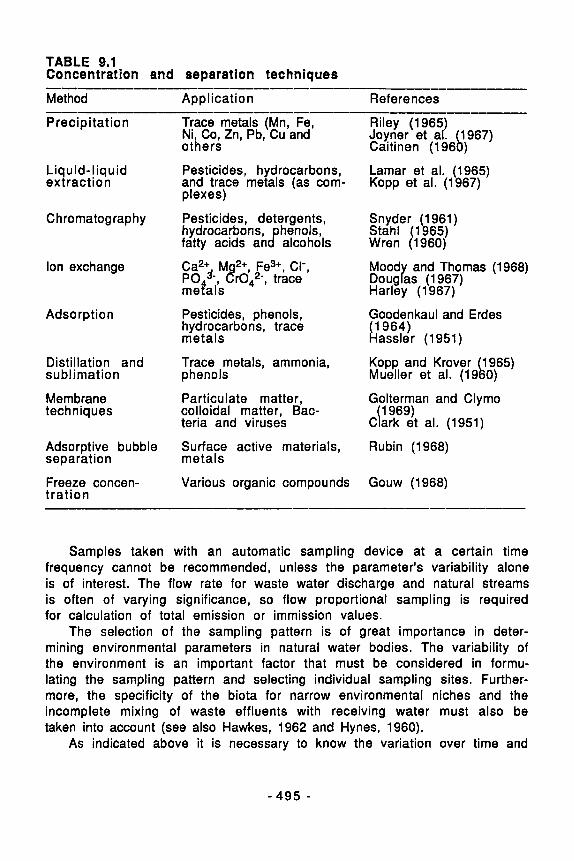
TABLE 9.1 Concentration and separation techniques

Precipitation

Liquid-liquid extraction

Chromatography

Ion exchange

Adsorption

Distillation and sublimation

Membrane techniques

Adsorptive bubble separation

Freeze concen- tration

Trace metals (Mn, Fe, Ni, Co, Zn, Pb, Cu and others

Pesticides, hydrocarbons, and trace metals (as com- p I ex e s)

Pesticides, detergents, hydroca!bons, fatty acids ancf?%%s

Ca2+ M *+, Fe3+, CI-, PO,^-, 8r0,2-, trace mefals - Pesticides, phenols, hydrocarbons, trace metals

Trace metals, ammonia, phenols

Particulate matter, colloidal matter, Bac- teria and viruses

Surface active materials, metals

Various organic compounds

Riley (1965)

Caitinen (196 6' ) 967) Joyner et at.

Lamar et al. (1965) Kopp et al. (1967)

Snyder (1961) Stahl 1965) Wren fi960)

Mood and Thomas (1968) Doug L s (1 967) Harley (1 967)

Goodenkaul and Erdes (1 964) kassler (1951)

Kopp and Krover (1965) Mueller et al. (1960)

Golterman and Clymo

Cark l1 969) et al. (1951)

Rubin (1968)

Gouw (1968)

Samples taken with an automatic sampling device at a certain time frequency cannot be recommended, unless the parameter's variability alone is of interest. The flow rate for waste water discharge and natural streams is often of varying significance, so flow proportional sampling is required for calculation of total emission or immission values.

The selection of the sampling pattern is of great importance in deter- mining environmental parameters in natural water bodies. The variability of the environment is an important factor that must be considered in formu- lating the sampling pattern and selecting individual sampling sites. Further- more, the specificity of the biota for narrow environmental niches and the incomplete mixing of waste effluents with receiving water must also be taken into account (see also Hawkes, 1962 and Hynes, 1960).

As indicated above it is necessary to know the variation over time and

- 4 9 5 -

place to be able to select the right sampling programme. So, whenever possible, the sampling programme should be based on a previous one or a pilot programme made prior to selection.

Preservation of sampfes is often difficult because almost all preser- vation methods interfere with some of the tests. Immediate analysis is ideal but often not possible. In many cases storage at low temperature (4°C) is the best method of preservation for up to 24 hours. No method of preservation is entirely satisfactory and the choice of which to use should be made with due regard for the measurements that will be required.

Some useful methods of preservation and their application are summa- rized in Table 9.2, but the selection of the right method is dependent on the measuring programme and general guide lines cannot be given.

TABLE 9.2 Methods of preservation

~

Methods Application

Storage at low temperature General Sulphuric acid pH 2-3 Nutrients, COD Formaldehyde Affects many measurements Sodium benzoate Sludge and sediment samples

Iodine 6; lgal counts

-_______-_---__--- -----

grease measurement)

-~ ----------- --~-----

9.2.2. Insoluble material.

P.9.3. Insoluble material covers the range from 0.01 - 200 pm in size. Colloidal particles are included as they range in size from about 0.01 - 6 pm. Particles smaller than 0.1 pm are classified as dissolved.

When waste water is examined, the filterable residue is determined by using different types of filters with a maximum pore size of 5 pm, so that colloidal particles are not included. When examining natural waters, analysis of the colloidal fraction and even determination of particle size distribution are often required. Methods available for such more detailed ecaminations are reviewed in Table 9.3.

An important measure for the determination of bioorganic and inorganic particles is the ability of the particles to accumulate material from the environment by absorption processes. The results of adsorption examinations are often expressed by means of adsorption isotherms. If adsorption is involved the following adsorption isotherms are generally applied.

- 496 -

Freundlich's adsorption isotherm

x = a * c b (9.1 1

La ng m u i rk adsorption is0 the r m

a * c k, + c

x P --

where a, k, and b = constants c = concentration in liquid x = concentration of adsorbent

TABLE 9.3 Methods for detailed examination of insoluble material

Centrifu ation X-ra dffusion Eleckon microscopy UV, visible and infrared spectroscopy Differential thermal analysis Optical microscopy Ion exchange Gel filtration Electrophoresis Sedimentation Dialysis

9.2.3. Biological oxygen demand.

The term BOD refers primarily to the result of a standard laboratory procedure, developed on the premise that the biological reactions of interest can be bottled in the laboratory and that the kinetics and extent of reaction can be observed empirically. The method is, however, relatively unreliable as a representation of the system from which the sample was taken. Therefore, the true worth of the standard procedure and the necessity for a more fundamental approach to measurements of biological reactions will be discussed here.

The basis difference between the BOD bottle and a stream is that the BOD bottle is a static system which is controlled to provide aerobic conditions, while the stream is a dynamic system which may include anaerobic areas due to formation of bottom deposition. As the synthesized microorganisms age, lysis of the cell walls occurs and the cell contents are released. The remains of the cell walls are relatively stable materials, such as polysacharides,

- 4 9 7 -

which are not degradated during 5 days, which is the normal duration of the BOD test (indicated as BOD,). Furthermore, ammonia may or may not be oxi-

dized to nitrate during this period through the action of nitrifying bacteria. The analytical procedure of BOD is based on the assumption that the

biological oxidation is a first order reaction. This assumption may, in many cases, be an oversimplification as the biological oxidation consists of independent steps: energy reactions, which support the synthesis of organic matter into new cells, and endogenous reactions.

The rate at which the biological processes occur is also a function of the food to organism ratio, so the rate of stabilization of organic matarial is therefore very much related to upstream activity. In addition the rate at which biological processes take place is strongly dependent on the flow pattern. Shallow streams normally provide an excellent food to organism potential because of their high velocity, which provides turbulence.

In conclusion, the BOD results obtained in a BOD bottle have a limited quantitative correlation with the oxygen demands present in waste water or aquatic ecosystems. However, BOD,, as presented in many books on standard

methods, is still used worldwide for determination of the oxygen consump- tion ofr biological and chemical oxidation of waterborne substances, despite the fact that the method is very time consuming and it takes 5 days to get the result.

Standard Methods (1 980) defines BOD, as determined in accordance with

the procedure presented in the bood as follows: The biochemical oxygen demand (BOD) determination described herein

constitutes an empirical test, in which standardized laboratory procedures are used to determine the relative oxygen requirements of waste waters, effluents and polluted waters. The test has its wides application in measur- ing waste loadings to treatment plants and in evaluating the efficiency (BOD removal) of such treatment systems. Comparison of BOD values cannot be made unless the results have been obtained under identical test conditions.

The test is of limited value in measuring the actual oxygen demand of surface waters, and the extrapolation of test results to actual stream oxygen demands is highly questionable, since the laboratory environment does not reproduce stream conditions, particularly as related to tempera- ture, sunlight, biological population, water movement and oxygen concen- tration.

Nitrification is a confusing factor. Procedures that inhibit nitrification are available, or corrections for nitrification can be carried out through nitrate determinations. The following methods for inhibition have been suggested: pasteurization (Sawyer et al., 1946), acidification (Hurwitz et al., 1947), methylene blue addition (Abbott, 1948), trichloromethyl pyridine addition (Goring, 1962), thiourea and allylthioureas addition (Painter et al.,

- 4 9 8 -

1963) and ammonium ion addition (Quastel et al., 1951 and Gaffney et al., 1 958).

If BOD, determinations are replaced by BOD curves, usefull information

about the carbonanceous oxygen demand may be obtained, but this technique requires 10 to 20 days and is complicated by the need for suitable seed organisms. Improved analytical procedures utilizing the dissolved oxygen probe make it possible to determing oxygen required for energy in less than one hour. The synthesis of biological material can be determined through enzyme activity measurements. Such analysis can be carried out in a few minutes.

Oxygen required during stabilization of synthesized cell material can be calculated once synthesis is known. In other words it is possible to arrive at a fundamental measurement of biological oxidation in less than one hour by summation of oxygen needed for energy and endogenous requirements. The result has been termed the stabilization oxygen demand.

Parallel measurements of COD (Chemical Oxygen Demand) and TUC (Total Organic Carbon) are good supplements to the BOD-determinations and thereby might eliminate some of the disadvantages of the BOD-determina- tion.

Often a statistical relationship is worked out for a specific stream between BOD and COD and TOC, to reduce the very time-consuming BOD analysis by translating COD or TOC to BOD.

The above developments have improved the application of oxygen demand measurements although the disadvangages have been only partially elimi- nated. BOD, is and will be for many years the most important measurement of water quality in spite of its disadvantages.

9.2.4. Chemical kinetics and dynamics in water systems.

Kinetic and dynamic studies deal with the changing concentrations of reactants and products is essentially unstable situations. This sets certain requirements for analytical procedures. Spectrophotometric and electro- metric methods are widely used in continuous monitoring of reactants or products. Many reactions of interest in water systems are not amenable to continuous monitoring and discrete samples must be taken for analysis. A variety of methods can be used to stop reactions in samples, for example by using inhibitors or poisons like trichloracetic acid, mercuric ions, form- aldehyde, heat, or even strong acids or bases.

P.9.4. The term kinetic analysis can be applied t o a rather diverse group of analytical procedures, which determine concentrations of substances by measuring the rate of a

- 4 9 9 -

reaction rather than the concentration itself.

The field of kinetic analysis is too broad for more than a cursory coverage here and the interested reader is referred to several review articles (Garrel and Christ, 1965; Stumm, 1967 and Faust and Hunter, 1967).

Table 9.4 gives a survey of some of the most commonly used kinetic analysis of water systems, with reference to the original literature.

TABLE 9.4 Kinetic analysis

Component Reference

Standard Methods 1980 or later editions) Glucose Hill and Kessler (1 61) ATP Patterson (1 970)

Patterson et al. 1970)

NADPH Kratochvil et al. (1967) Nutrients (low level) Grouch and Malmstadt 1967) Ammonia Mn2+/M no2

--- ___- -~___- - 6 52-, so,2-

Hamilton and Ho 1 m-Larsen (1 967)

Weichelbaum et al. (19 b 9)

--- Morgan and Stumm (1965) - - - - ~ -

9.2.5. Analysis of organic compounds in aqueous systems.

All waters contain measurable concentrations of organic matter, which has originated from natural processes of biological synthesis and degra- dation or from the various activities of man.

Distinction can be made between the presence of specific organic compounds, such as alkyl benzene sulphonates, herbicides, insecticides etc., the presence of compounds of a less well defined nature that cause dye, taste and odour problems, and the presence of organic compounds which at present are not associated with known problems. The latter situation requires that the analyst identify and estimate all organic compounds in a dilute aqueous solution and/or suspension, which would, of course, be an impossible task. There are, however, a number of approaches to this problem. One is to guess from knowledge of discharges and previous experience what organic compounds might be present, and then to examine the mixture of these. Another possibility is to detect and estimate classes of materials, rather than individual compounds. Typical examples of classes are carbohydrates, amino acids, ketones, etc.

Several identification methods are available for detecting classes of organic compounds. Among the physical methods should be mentioned determination of the refractive index, magnetic susceptibility, absorption spectra, fluorescense spectra, Raman spectra, mass spectra, NMRS (Nuclear

- 500 -

Magnetic Resonance Spectra), X-ray diffraction, specific dispersion, dielectic constants and solubility. Chemical identification includes the determination of the molecular weight, elemental analysis and estimations of functional groups. For further information, see Hunter (1962); Lee (1965); Mitchell (1966).

Within the analysis of specific organic compounds, that of pesticides and PCB is of great importance, and some guidelines for the estimation of these compounds should be given.

The general procedure consists of three steps: 1. Concentration of samples. 2. Cleaning up. 3. Ident i f icat ion of pesticides and their metabolites.

For the first step adsorption on activated carbon or liquid-liquid extrac- tion can be used. Relatively unpolluted waters may not require an extensive cleanup since pollutants would be of minor importance, but due to the small concentrations present in unpolluted waters the concentration step is required. Adsorption is a very useful method for this first step, as it is able to handle a large volume of water at low concentrations. Its limitation is that it is not quantitative and it is necessary to correct the result by using a recovery percentage. The conditions used for serial liquid-liquid extractions of various pesticides are summarized in Table 9.5, and, as can be seen, a wide range of organic solvents is used for this purpose.

Pollutants may originate from domestic and industrial waste water and a cleanup step is therefore necessary. The following cleanup techniques are in general use:

1. Partition chromatography on silicid acid columns for removal of more or less identified organic matter, including organic dyes (see Hinding et al., 1964; Epps et al., 1967; Aly and Faust, 1963).

2. Thin fayer chromatography for separation of organic pollutants in the analysis of chlorinated hydrocarbon pesticides (Crosby and Laws, 1964).

3. Adsorption on an aluminia column for removal of pollutants in identification of chlorinated hydrocarbons (Hamence et al., 1965)

4. Countercurrent extraction for identification of organic pesticides in food.

5 . A single-sweep codistillation method for general removal of organic pollutants (Storherr and Watts, 1965).

For the identification of organic pesticides and their metabolites either thin layer chromatography or gas-liquid chromatography are mainly used.

- 5 0 1 -

TABLE 9.5 Condltlonr used for serlal Ilquld-llquld extraction of pestlcldes from aqueous samples

Sample Solvent Pesticides Solvents volume volume

(ml) (ml)

Mean

( % I Ptl recovery

DDT Dieldrin and metabolites

Five CH

Eight CH Aldrin Aldrin Eleven CH Heptachlor

Five CH Nine CH Three CH Four CH Three CH Parathion and diazinon

Dipterex and DDVP Malathion Diazinon Abate Parathion Methyl parathion,

3:l Ether:n-hexane n-Hexane

1 :1 Ether:pet.elher,

n-Hexane 1:l Benzene:hexane 1:l Ether:hexane n-Hexane 2:l Petather: iso- propyl alcohol n-Hexane Benzene n-Hexane 1 :1 n-Hexanmther n-Hexane 1 :1 Ether:pet.ether or CHCl3

Ethyl acetate Dichloromethane Benzene Chloroform Benzene Benzene

CHCl3

diazinon, malathion, azinphos-meth yl

parathion, baytex

parathion

Parathion, methyl n-Hexane

Parathion, methyl 1 :1 Hexane:ether

Dursban Dichloromethane

1500 100

1000

1000 850 850 12

1000

1000 250

1000 100

1000 1000

50 ? 100

1000 1000

250

1000

100

50

250,200,150,150 4.0-5.0 4 * 50

100. 4 50

2 25 100, 4 50 100, 4 50

150, 3 * 75

5 0 25 3 0

100 Acid

3 ' 2 7.0

3 * 100

100, 4 50

50, 25 8.0

100 50, 25, 25 1 .o 500 Acid 2 5 ?

3 30 7.0-8.0

100 Acid

3 100

100, 50

88a0 61b 90-95

88

80-115 43.4 69.6 2.3-106.0 8 0

9 5 84.6-1 01.8 9 5 97-1 00 > 90 9 0

94.5 100 ?

7 0 99-1 00 95.3-99.7

> 90

9 8

9 2

a) Interferences absent. b) Interferences present.

References 1. Berck (1953); 2. Cueto et al. (1962); 3. Weatherholtz et al. (1967); 4. LaMar et al. (1965); 5. Kawahara et al. (1967); 6. Cueto et al. (1967); 7. Weatherholtz et al. (1967); 8. Holden et al. (1966); 9. Pionke et al. (1968); 10. Wheatly et al. (1965); 11. Beroza et al. (1966); 12. Warnick et al. (1965); 13. Teasley et al. (1963); 15. Mount et al. (1967); 16. Kawahara et al. (1967); 17. Wright et al. (1967); 18. Mulla (1966); 19. Pionke et al. (1968); 20. Warnick et al. (1965); 21. Teasly et al. (1963); 22. Beroza et al. (1966); 23. Rice et al. (1968).

14. El-Refai et al. (1965);

- 502 -

9.2.6. Analysis of inorganic compounds in aqueous systems.

Water can be considered in three categories from an analytical point of view:

1. Surface water and ground wafers, which are usually very dilute solutions containing several species of cations, anions and neutral organic and inorganic compounds.

2. Seawater , which contains several ions in high but constant concen- 1 tration.

3 . Waste waters, which cause special problems because of their variable composition and high concentrations of suspended matter.

, groups:

The inorganic substances to be considered can be classified into two

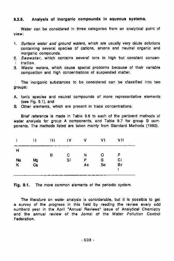
A. Ionic species and neutral compounds of more representative elements (see Fig. 9.1), and

B. Other elements, which are present in trace concentrations.

Brief reference is made in Table 9.6 to each of the pertinent methods of water analysis for group A components, and Table 9.7 for group B com- ponents. The methods listed are taken mainly from Standard Methods (1980).

I I I I l l I V V V I V I I

H B C N 0 F

Na MI Si P S CI K ca As Se Br

I

Fig. 9.1. The more common elements of the periodic system.

The literature on water analysis is considerable, but it is possible to get a survey of the progress in this field by reading the review every odd numberd year in the April "Annual Reviews" issue of Analytical Chemistry and the annual review of the Jornal of the Water Pollution Control Federation.

- 5 0 3 -

TABLE 9.6 Analysis of inorganic compounds (group A) ------ -------

S.M. = Standard Methods (1980) Lowest measurable

Element Reference concentration ------I---I__--___- -- A S S.M., spectrop hotometry 20 PPb B S. M. , spectrophotometry 0.1 ppm Br S. M., spectrophoto metry 0.1 pprn

Br Fishman and Skougstadt (1 963) 5 PPb

ca S.M., titration 1 PPm C02, C032- S.M., titration 1 PPm

CI' S.M., titration 1 PPm

I- S.M., spectrophotornetry 1 PPb

spectrophotornetry

CN' S.M., spectrophotometry 0.02 ppm

F- S .M., spectropho tometry 0.1 ppm

w S.M., spectrophotometry 0.5 ppm NH,+ S.M., spectrophotometry 0.01 ppm

NOi S.M., spectrophotomatry 1 PPb NO,- S.M., spectrophotometry 2 PPb 0 2 S.M., titration 0.1 ppm p o p S.M., spectrophotornetry 0.01 ppm K Si

S.M., spectrophotometry S.M., spectrophotometry

Na S.M., gravimetric

S2- S.M., spectrophotometry so,2- S.M., turbidirnetric

S.M., flame photometry

5 PPm

1 PPrn

0.02 pprn

0.01 ppm 0.05 ppm

0.5 ppm

In view of the present-day emphasis on instrumental methods of analysis based on application of physical properties, it is interesting that the traditional methods still predominate among the standard methods in water analysis of group A compounds. Only about 20 per cent of the methods described in Standard Methods (1980) for these compounds are purely instrumental, without extensive chemical pretreatment. The traditional mehods prevail, including spectrophotornetric methods with extensive chemical pretreatment, because they have proven trustworthy and well suited to the sensitivities and precision required.

- 5 0 4 -

TABLE 9.7 Analysis of inorganic compounds (group B)

sample

--------- -----I_- - Methods Applications

1

Flame photo rnetry

Atomic absorption spectrophotometry (AAS) K, Rb, Sc, Ag, Na, Sr, V, Zn

Atomic fluorescence Same as AAS spectrophotometry

Emission All metals spectrophotometry

Adsorption Almost all elements spect rop hotornetry

X-ray spectroscopy

Activation analysis

Li, Na, K, Ca, Mg, Sr, Ba

Al, Cd, Ca, Cr, Co, Cu, Fe, Pb, Mg, Mn, Hg, Mo, Ni,

--- ---------I-__-

--- -------~-__-

a ---- ----

-- --- -------_I--__

All elements from Na up in the periodic table

As, Ba, Be, Br, Cs, Cr, Co, Cu, Au, M , In, Mn, H Ni, P, Ce, Re, R, Ru, Na, Sr, S, Ta, Tf Th, W, V, ?!n

- ~ - - ~ - - - ~ - _ _ -

----I- ------------__-

t Absor- bance

- Addition mg I-'

Conc. sample

- Addition mg I-'

Conc.

Fig. 9.2. Application of "the addition method".

- 5 0 5 -

Group B compounds are more widely analysed by use of instrumental methods, as these are better suited to estimation of minor concentrations. Often the so-called standard addition method must be used to eliminate pollutants. The method is illustrated in Fig. 9.2.

9.2.7. Bacterial and viral analysis of water.

Natural water free from pollution has a rich microflora. Algae, diatoms, phytoflagellated, fungi, protozoans, metazoans, viruses and many genera of bacteria; including Alcaligenes, Caulobacteria, Chromobacterium, Flavo- bacterium, Micrococcus, Proteus and Pseudomonas. Sulphur, nitrogen fixing, denitrifying and iron bacteria may be found, depending on the substrate concentration. The microflora are generally strongly affected by solar radia- tion, temperature, pH, salinity, turbidity, hydrostatic pressure, dissolved oxygen (the redox potential), the presence of organic and inorganic nutrients, growth factors, metabolic regulating substances, and toxic substances.

P.9.5. Water is one of the most important media for trans- mission of human microbial diseases and some of the best known examples include typhoid fever, paratyphoid fevers, dysentery, cholera and hepatitis.

It is generally accepted that the addition of pollutants to water may be actually injurious to the health and well being of man, animals and any aquatic life. Intestinal micro-organisms from man and warm-blooded animals enter rivers, streams and large bodies of water. Among these microbes the coliforrn group are most frequently present in water samples, which explains why they are often used as bacterial indicators, although far from ideal.

However, a wide variety of pathogenic bacteria may also be noted in water samples, such as Brucella, Leptospira, Mycobacterium, Salmonella, Shigella and Vibrio.

A number of biological measurements are made to assess the bacteriological quality of water and thereby indicate the presence or absence of pathogenic enteric bacteria. Standard Methods (1 980) contains a number of relevant methods.

The frequency of sampling to determine the bacteriological quality of drinking water is dependent on the size of the population served; however, two samples per month must be considered as the minimum. A sample frequency of one per day is recommended for a population of 25,000 inhabitants.

Fecal Coliform criteria are widely used for recreational waters and in

- 5 0 6 -

Table 9.8 is shown an example (Water Quality Criteria (1968)).

TABLE 0.8 Criteria for recreation waters

Water usage Fecal Coliform bacteria/lOO ml ----

General recreation Average < 2000

Designated for recreation

Primary contact log mean not to exceed 200 recreation

Maximum < 4000

log mean not to exceed 1000 Maximum 10% of samples > 2000

Maximum 10% of samples > 400

Viral analysis of water and waste water requires special equipment and techniques, and only a few laboratories are equipped to carry out such analyses. (Further details of these procedures, see Rhodes and van Ruoyen, 1968; Vorthington et al., 1970; England et al., 1967).

More than 100 human enteric viruses, the most important infective viral agents in water, have been described in the literature.

A review of human enteric viruses and their associated diseases is given in Table 9.9.

TABLE 9.9 Human enteric viruses and their associated diseases

Diseases Number of types Associated diseases __------------- ----

Polio virus 3 Paralytic polimyelitis, menigitis

Coxsackie virus A 26 Coxsackie virus B 6

Herpangina, menigitis Pleurodynia, menigitis and infan- tile myocarditis

Infectious hepatitis 1 Hepatitis

Adeno virus 30 Eye and respiratory infections

Reo virus

Echo virus

3

29

Diarrhoea, fever, respiratory infections

Menigitis, respiratory infections, fever and rash

- 507 -

9.2.8. Toxicity of bioassay techniques.

For more than 100 years test organisms have been used to establish the toxic effects of water pollution (Penny and Adams, 1863). Such investi- gations indicate the degree of dilution andlor treatment that must be provided to prevent damage to the organisms in the receiving waters. Fish, invertebrates and various algae have been variously used for this purpose.

At one time it was hoped that the toxicity of wastes to aquatic organisms could be determined by an analysis of the chemical constituents and comparison with a table listing the toxicities of the various waste substances to fish and other aquatic organisms, and thereby assess the toxicity level. However, this goal has not proved entirely feasible due to the following:

1.

2.

3.

Although a great many toxicity data have been recorded (see Jsrgensen et al., 1979), information is still limited in comparison with the number of toxic substances and species present in aquatic ecosystems.

Tests reported in the literature might have been carried out u n d e r conditions different to those in the ecosystem concerned: pH, dissolved oxygen, salinity, temperature and several other parameters profoundly affect the result of toxicity tests.

The presence or absence of trace components - often impossible to test in detail - also significantly affect the results.

However, information on the presence of chemical constituents and the related toxicity data found in the literature can be of great value in the interpretation of toxicity bioassay - in practice the two methods of determining the toxicity of waste should be used side by side.

Toxicity bioassay experiments on fish are widely used all over the world, although other vertebrates, invertebrates and algae are also used (see Veger, 1962; Anderson, 1946 and 1950; Gillispie, 1965).

The last five editions of Standard Methods for the examination of Water and Waste Water (WPCF), contain detailed information on toxicity bioassay methods on fish, including selection of test fish (species and size), their preparation (acclimatization 10-30 days, feeding etc.), selection and preparation of experimental water dilutions and sampling and storage of test material. Furthermore, it provides guidelines for general test conditions: temperature, dissolved oxygen content, pH, feeding, test duration, etc.

Procdures for continuous-flow bioassays are also available (see Stand- ard Methods, 1980) and the basic components are shown in Fig. 9.3.

- 5 0 8 -

Diluent water u ,Heating equipment

Toxicant supply

I.' 1;";*t

container

Fig. 9.3. Continuous-flow bioassay.

P.9.6. The ultimate aim of the bioassay test is to find TL,, or LC,,, the concentration at which 50 per cent of the test fish survive.

This value is usually interpolated from the percentages of fish surviving at two or more concentrations, at which less than half and more than half survived. The data are plotted on semilogarithmic coordinate paper with concentrations on logarithmic, and percentage survival on arithmetic scales. A straight line is drawn between the two points representing survival at the two concentrations that were lethal to more than half and to less than half the fish. The concentration at which this line crosses the 50 per cent survival line (see Fig. 9.4) is the TL,, or LC,, value. (Other methods of determining this value are sometimes more satisfactory).

A precision within about 10 per cent is often attainable, but better precision should not be expected even under favourable circumstances. In most cases 48-hour and 96-hour values are also determined, but these concentrations do not, of course, represent values that are safe in fish habitats. Long-term exposure to much lower concentrations may be lethal to fish and still lower concentrations may cause sublethal effects, such as impairment of swimming ability, appetite, growth, resistance to disease and

- 5 0 9 -

reproductive capacity. Formulae for the estimation of permissible discharge rates or dilution ratios for water pollutants on basis of acute toxicity evaluation have been tentatively proposed and discussed (see Henderson, 1957; Warren and Doudoroff, 1958).

Conc. 321 a

32- Conc.

(eg. mg I I 16-

8-

4-

2-

1 20 LO 60 80 100 Yo

Test Animals,surviring%

Fig. 9.4. Interpretation of toxicity bioassay results.

A widely used method employs fractional application factors by which the LC,, values can be multiplied until a presumably safe concentration is

arrived at. However, it would seem that no single application factor can be applied to all toxic materials. The National Technical Advisory Committee on Water Quality Requirements for Aquatic Life has tentatively grouped toxi- cants into three main categories according to their persistance (see Federal Water Pollution Control Administration, U.S., 1968). This solution to the pro- blem must only be considered as provisional, however, and possible syn- ergistic and antagonistic factors should always be taken into consideration.

The effects of the presence of two or more toxicants in the water being

- 5 1 0 -

tested may be calculated by the following equation:

where C,, C, ....... = the actual concentrations TL,,, TLm2 ....... = the corresponding threshold limits ST = the sum of the effects

The value of ST, whether > or c than one, is determined. This method can be applied, provided that no knowledge on synergism and

anatgonism is available.

9.2.9. Measurement of taste and smell.

Direct measurement of material that produces tastes and odours can be made if the causative agents are known, for instance, by gas or liquid chromatography.

Quantitative tests that employ the human senses of taste ans smell can also be used, for instance, the test for the threshold odour number (TON). The amount of odorous water is varied and diluted with enough odour-free distilled water to make a 200 ml mixture. An assembled panel of 5-10 "noses" is used to determine the mixture in which the odour is just barely detectable to the sense of smell. The TON of that sample is then found, using the equation

A + B TON 7 (9.4)

where A is the volume of odorous water (ml) and B is the volume of odour-free water required to produce a 200 ml mixture.

9.2.10. Standards in quality control.

P.9.7. A standard i s a definite rule or measure established by authority. It i s official, but not necessarily rationally based on the best scientific knowledge and engineering practice. Standards can be applied either on receiving waters - rivers, lakes, estuaries, oceans or groundwater - or on the effluent from municipal, industrial and

- 5 1 1 -

agricultural pursuits.

Receiving water standards reflect the assimilative capacity of the water body receiving effluents.

Their purpose is to preserve the water body at a certain minimum quality. Effluent or emission standards are easy to administer, but do not take into account the most economic use of the assimilative capacity of receiving waters.

P.9.8. Use of concentration effluent standards for a substance can easily be misleading since dilution can mask the true pollution level. It is more appropriate to limit the amount of pollutant, that can be discharged in a given time, e.g. kg per day, week or month.

A relationship between the two types of standards is difficult to estabilsh. It requires knowledge of the complex relationship between the discharge and the ultimate concentration in the receiving water, and since almost all discharged components are involved in many processes in the aquatic ecosystem, the problem must be solved by systems analysis (see the section on ecological models in 1.5).

Standards for receiving waters attempt to protect the water resource for uses such as drinking, swimming, fishing, irrigation, etc. However, standards should not be set at minimum levels, lests water quality be destroyed for future generation, but should prevent a polluter from profiting at the expense of neighbouring water users and compensate for differences in summer and winter and dry versus wet years, etc.

The use of water resources directly determines the standards applied to receiving waters and indirectly determinies those applied to effluent.

Table 9.10 illustrates how standards can be set for different water usage. Although it includes only a limited number of items, it may be considered representative of standards applied to fresh surface waters.

A major source of pollution is the municipal waste water. It is the responsibility of the municipality to construct facilities to meet the standards, but design and construction of a waste water treatment plant is only the first part of an extensive pollution abatement programme. The plant must be operated to meet the design objectives and, therefore, proper operation and maintenance will require additional funds. Furthermore, an effluent standard should be set for every plant to ensure it is functioning as represented to the taxpayers, and the key to this will be the monitoring of treated effluent.

- 5 1 2 -

TABLE 9.10 Examples of standards

Class A B C D --------------------

Best usage Drinking water s u pp I y

Sewage or None, which waste is not effec- effluent tively disin-

fected

w 6.5 - 8.5

Dissolved oxygen 25.0 mg I-'

Bathing Fishing Ag r icu It u r al

None, which is not effec- tively disin- fected

Industrial

6.5 - 8.5 6.5 - 8.5 6.0 - 9.5

25.0 mg I-' 25.0 mg I-' 13.0 mg I-'

The other major source of pollution, industrial waste water, is another problem. Industries usually have little reason to devote money to waste treatment without tremendous pressure form all levels of government and the general population.

Finally funds must be used for monitoring and surveillance of standards of receiving waters in order to control the water quality and to assess the success of control methods.

9.3. EXAMINATION OF SOLIDS.

9.3.1. Pretreatment and digestion of solid material.

Procedures intended for the physical and chemical examination of waste waters and waters can also be applied in most cases to examination of soil, sludge, sediments and solid industrial waste, after suitable pretreatment. Standard Methods (1 980) gives details on pretreatment procedures for sludge and sediments, and these are generally applicable with some minor modification, to all types of solid material. Some problems related to the examination of solid material should be mentioned, however: 1. representative samples are very difficult to obtain, but a fixed

procedure cannot be laid down because of the great variety of conditions under which collection must be made. In general the sampling procedure must take into account the tests to be performed and the purpose for which the results are required,

2. determination of components that are subject to significant a n d unavoidable changes on storage cannot be made on composit samples, but

- 5 1 3 -

should be performed on individual samples as soon as possible after collection or preferable at the sampling point,

3 . preservation of samples is often difficult because most preservatives interfere with some of the tests. Chemical preservation should be used only when it can be shown not to interfere with the examination being made. Storage at a low temperature (0-4°C) is often the only way of preserving samples overnight.

As mentioned, a pretreatment is usually necessary before the standard procedures used for water and waste water assessment can be used on solid material. Digestion of samples are necessary before determination of total concentration. The digestion procedure is dependent on the component to be analyzed, as it must be certain that the total amount is dissolved.

9.3.2. Examination of sludge.

P.9.9. The control of sewage treatment is dependent on tests on sludge. This control is of special importance in the activated sludge process, where the sludge parameters determine the operation of the plant.

Tests for the various forms of residue determine classes of material with similar physical properties and similar responses to ignition. The following forms of residue are widely used in the examination of sludge, and also for soil samples:

1.

2.

3.

4.

5.

6.

Total residue of evaporation. The procedure (Standard Methods, 1980) is arbitrary and the result will generally not represent the weight of actual dissolved and suspended solids. A discussion of the temperature for drying residues can be found in Standard Methods (1980), but 103°C is generally applied. Total volatile and fixed residue is determined by igniting the residue on evaporation at 550°C in an electric furnace to constant weight. Total suspended matter is determined by filtration. The amount of suspended matter removed by a filter varies with the porosity of the f i l ter . Volatile and fixed suspended matter are determined by evaporation and ignition of the suspended matter obtained under point 3. Dissolved matter is calculated from the difference between the residue on evaporation and the total suspended matter. Matter may be reported on either a volume or a weight basis.

- 5 1 4 -

Additionally two indices are used to estimate the various forms of residue. The so-called sludge volume index, which is the volume in ml occupied by 1 g of activated sludge after the sludge has been allowed to settle for 30 minutes. The sludge density index, which is the reciprocal of the sludge volume index multiplied by 100.

9.3.3. Examination of sediments.

P.9.10. Analyses of sediments are widely used for environmental control, because sediment is able to accumulate various pollutants. Significantly higher concentrations of toxic organic compounds and heavy metals are found in the sediment than in the overlying water.

Therefore, more accurate mapping of the pollution is achieved by examinating the sediment than the water. Sediment is able to bind contaminants by adsorption, biological uptake of benthic organisms and chemical reactions, for each of which it is often important to find the binding capacity and its allocation, in order to predict the ecosystem’s future reaction to pollution. However, this involves a rather time-consuming examination of the chemical and biological composition of the sediment. Kamp-Nielsen (1 974) has described a quicker but empirical method for determining the nutrient binding capacity of sediment, which can be expanded slightly to cover toxic compounds and heavy metals.

Examination of sediment also has the advantage that sediment has memory. Analysis of a sediment core taking samples at various depth can give clues to previous conditions in the ecosystem by determination of the net settling rate expressed, e.g. in cm per annum.

Fig. 9.5 illustrates the results of such an analysis. The digestion methods used on sludge, can also be applied to sediment. It

is often necessary to use the most complicated digestion methods if determination of the total content is required. However, from an environmental management point of view, it is generally sufficient to use simpler digestion methods, as these give only slightly lower results. For example, to determine the heavy metal concentration in sediment it is often sufficient to use wet chemical digestion by nitric acid. The difference between this method and the use of sodium carbonate melting as pretreatment to an extraction with hydrogen fluoride and nitric acid is only minor and will always represent only very non-labile material (see Nordforsk, 1975).

- 5 1 5 -

matter

Fig. 9.5. Metal anal sis of a core from Lake Glumsoe. Zinc and lead (mg/kg dry matter) are plotte d against the depth.

9.4. EXAMINATION OF AIR POLLUTION.

9.4.1. Introduction.

The prevalent air pollution at a given time is a function of a number of factors, which may be categorized as follows:

1. Meteorological conditions 2. Source strength and position 3. 4. Deposition and/or decomposition rate

Quantitative composition of source emission

P.9.11. A complete characterization of the total immission is practically impossible, and indeed any given air pollution description is only a reflection of the actual true immis- sion,

i.e. it is limited in several ways with respect to number of analysed compounds, knowledge of statistical variation in time and space ans analytical problems of a prectical and/or theoretical nature. Consequently, it is necessary to define as precisely as possible the aim of the examination of

- 5 1 6 -

the air. Is the purpose only to monitor the major pollutants in quantity or to gain knowledge about the distribution of these compounds with major adverse effects on human health, plants and animals and/or materials? In other words: choice of immission component and preliminary determinations of concentration range are prerequisite.

Table 9.11 lists the most commonly measured air pollutants and typical ranges in American and British cities. It is of interest that only a very limitied number of these compounds have not been present in the atmosphere during the period of mans presence on earth (compare with Table 9.12).

These few compounds originate mainly from the organic chemical industry and include halogenated aromatics (DDT, PCBs) and polyaromatics (PAH) .

P.9.12. The present air pollution is more a matter of quantitative than qualitative change, and a number of living organisms have actually been shown to possess potential adaptivity towards this new situation.

Similarly, it is within reach of modern technology to produce less corrosive materials in order to prevent damage due to air pollution.

Man, however, is subject only to very slow evolutionary change, and will certainly not develop within only a couple of hundred years.

In conclusion, therefore, it makes sense to focus on protecting human health when considering air pollution control and indeed this is common practice.

TABLE 9.11 Most commonly measured Air Pollutants

A. Composition of the atmosphere (Bowen, 1966) lll_~--------I-------__

Compounds pg/m3 STP Residence time (year)

600,000 36 - 90

3 - 30 2.99 10’

0 - 100 9.73 * 10’0

3 104 - 3 * 107

0 - 1 5 500 - 1200 0 - 6

4

0.027 0.1 1

2

short 4

short 0.014 0 - 50

-517 -

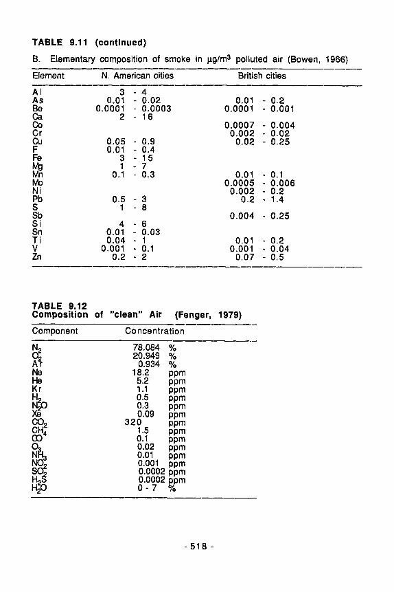
TABLE 9.1 1 (continued)

B. Elementary composition of smoke in pg/m3 polluted air (Bowen, 1966)

Element N. American cities British cities - -- ----------____-

A l As Be ca

i e

# Mo Ni Pb S Sb S i Sn T i v zn

3 - 4 0.01 - 0.02

0.0001 - 0.0003 2 - 16

0.05 - 0.9 0.01 - 0.4

3 - 15 1 - 7

0.1 - 0.3

0.5 - 3 1 - 8

4 - 6 0.01 - 0.03 0.04 - 1

0.001 - 0.1 0.2 - 2

0.01 - 0.2 0.0001 - 0.001

0.0007 - 0.004 0.002 - 0.02 0.02 - 0.25

0.01 - 0.1 0.0005 - 0.006

0.002 - 0.2 0.2 - 1.4

0.004 - 0.25

0.01 - 0.2 0.001 - 0.04

0.07 - 0.5

TABLE 0.12 Composition of "clean" Air (Fenger, 1979)

Component Concentration ---- - 78.084 Yo 20.949 Yo

0.934 Yo

N2

18.2 ppm Ne He 5.2 ppm Kr 1.1 ppm H 0.5 ppm

0.3 ppm 0.09 ppm xe

320 PPm 1.5 ppm 0.1 ppm 0.02 ppm 0.01 ppm 0.001 ppm 0.0002 ppm

3

bk

3 co,

;.y ly

- 5 1 8 -

Finally, two important aspects of the impact of air pollution on human health must be stressed. First is the traditional separation between outdoor and indoor ambient air quality, which has different acceptable limit values for pollutants.

Secondly, a distinction between indirect and direct effects has to be made; the current anxiety about heavy metals is partly due to direct effects (e.g. organic lead compounds in the city atmosphere), partly to accumulation with time in solids, plants and animals, which may result in elevated levels in foodstuffs. Equally, sulphur dioxide in combination with suspended particulate matter is directly toxic to humans at rather high concentrations; but the long-term indirect effects of this compound are also a matter of concern, as decreasing pH and increasing leaching of inorganic components of the soil - some being rather toxic, e.g. Al compounds - are detrimental to fresh- and groundwater systems. Bearing the above introductory statements in mind, the aim of an framework for air pollution examination should be clearer.

9.4.2. Meteorological conditions.

P.9.13. A detailed knowledge of the meteorological conditions is necessary in order to employ any emission measurement for environmental protection, because transportation from any source to the receptor is a function of meteo- rological variables. Furthermore, under certain meteoro- logical circumstances, a build-up of pollutants take place, even if the source strength remains constant. (Principles 2.1 and 2.6 are used).

The dispersion of air pollution from a point source as a function of different tropospheric lapse rate conditions (Fig. 8.2) can be represented by aplume from one chimney, see also section 2.11.

Fig. 9.6 shows the relative frequency of the different conditions in an open country, such as Denmark. Several larger cities of the world apply an early warning system involving meteorological data describing the lapse rat e conditions. In Denmark, this has not been necessary. The meteorological situation giving the highest ground level concentrations is inversion (see also 8.2.4). Inversions may occur for a number of reasons, the most important being: 1. (Fig. 9.7) strong cooling of the soi//concrete surface overnight (clear

sky), which results in the formation of a very sable layer close to the ground; during the day this inversion is often eliminated as the sun heats up the atmosphere.

- 5 1 9 -

%

50

LO

30

20

0

0

I \ I ,

I , I \ L c f T N G I

>

JAN FEB MAR APR MAV JUN JW AUG SEP OCT NOV DEC

Fig. 9.6. 60 meter stack. (Perkins, IJ’4) .

Frequency of t es of stack-smoke behaviour (1962-1964) for a

2. (Fig. 9.7) subsidence inversion. During high pressure situations, cold air with high density subsides and forms stable layer close to the ground with a rather small mixing height.

3. Front inversion. During the pregression of a front, the cold surface atmospheric layer is gradually covered or replaced by warmer air, and consequently the mixing height is reduced.

4. Sea-land breeze inversions (Fig. 9.8). Cities close to the sea are subject

- 5 2 0 -

to a special phenomenon due to the time lag difference in heating and cooling the concrete of a city compared wiht water. The net results is a seaward breeze at night and a land-ward breeze during day, the effect being most obvious on sunny days in the midafternoon.

These inversion situations may be modified by environmental factors, such as the presence of large amounts of concrete in a city resulting in a local air circulation system as shown in Fig. 9.9.

I \ A COMBINATION OF BOTH CASES

15C METERS

z

TEMPERATURE

T T

(b 1

Fig. 9.7. Temperature inversions. (a) During the day. (b) The sinking of air leads to warmin aloft, the formations of inversions. (c) A combination of cases. (Perkins, f974).

As industrial areas are often situated in the city periphery the inflow of air from here may increase the immission of some pollutants in the city centre.

In principle, the immission around a point source may be calculated on the basis of source strength, emission characteristics (such as stack height, smoke temperature, etc.) and meteorological parameters (see section 2.1 1). Even larger areas, like cities, may be treated in a similar way, but the presence of a large number of sources (point-, line- and area sources)

- 5 2 1 -

defined by the following examples: point source: a chimney, a vehicle, line soruce: a highway, area source: a city, an industrial area,

make it necessary to rely upon rather more empirical relationships, and the data therefore become less reliable. At present emission-based model calculations have not been able to replace field measurements of immission, and a combination of the two approaches will probably be a must for a long time yet.

A@\ ' I \ ' T>

WARM A I R

OCEAN ORLAKE LAND

Fig. 9.8. Sea breeze during the day. (Wright and Sjessing, 1976).

Before turning to a description of the most common air pollutants and the examination of their occurrence, it is relevant to stress a final point related to the aim of monitoring programmes.

P.9.14. It is generally not possible to conclude anything defini- tive with respect to harmful effects on living organisms due to immission exposure. Of course, the bases for limit values are controlled experiments, but their results may only rarely be translated directly to field conditions.

This is because: 1 . organisms exhibit a complex dose-response relationship (Fig. 9.1 O ) , see

also section 2.13, 2. synergistic/antagonistic effects are common.

In conclusion, this points to the necessity of introducing effect moni- toring using sensitive indicator organisms as a part of any environmental surveillance programme.

-522 -

- EZS-

9.4.3. Gaseous air pollutants.

SO, is one of the major gaseous air pollutants emitted from power plants

and industries. Some of the strongest air pollutions have been recorded around, e.g. Zn and Cd smelters, when sulphide ores are roasted to produce these metals. The results were heavy emissions of SO, that devastated the

environment, in particular the growth of trees and herbaceous plants. Fortunately, such strong emissions occur in only a few places; a larger problem occurs with the SO, produced during combustion of sulphur- containing fossil fuel, see also 8.4.1 and 4.7. This results in local as well as regional pollution problems.

Very often, the SO, is emitted together with particulates, and this

combination of suspended matter and SO, may cause health problems in

cities and industrial areas. SO, alone is not believed to be very harmful to man at its actual ambient levels. Regional pollution problems due to SO, are

mainly a result of its acidifying effects (see section 4.5). However, the acidification is also due to the presence of NO, and acidic

rain, which reacts with water as follows

2N0, + H,O * NO,- + NO; + 2H+.

I t is believed that the contribution to the total acidification of precipitation from NO, will increase during future decades as the immission

of NO, increases at present, the major part of the pH decrease is attributed

The measurement of SO, and SPM (Suspended Particulate Matter) in the

atmosphere is often performed with a so-called "OECD-instrument". Several other methods are available, and some of them permit an instantaneous reading, an important facility, when describing the immission in an area subject to very strong fluctuations with problematically high short-time peak values.

The design of the monitoring network and choice of equipment depend on the following factors.

First, effective design can only be made on the basis of some prior knowledge about the distribution of the pollutant within the area. The statistician needs to know pilot values about the variation in time and space in order to calculate the necessary number of measuring points. Often, however, practical and economic reasons limit the possibility of setting up an optimal network.

to so,.

- 524 -

Fig. 9.11. Frequency distribution of sulphur dioxide levels in selected American cities. 1962 to 1967 (l-hour averaging time). The approximate log normality of the distribution of sulphur dioxide concentrations is shown by the rather straight lines of the distribution functions when these are plotted on a logratihmic scale (concentrations) against a normal frequency. (Perkins, 1974).

Second, as regards choice of equipment, the kind of data required by the administration limit the number of feasible possibilities. Typically, a set of data for management purposes is defined in relation to the legislation, which may mean definitive averaging times, concentration ranges and analytical variation, the reason being that peak values and their frequency of occurrence are extremely important in relation to human health and plant damage. In order to estimate and thus control the peak value frequency, the

- 525 -

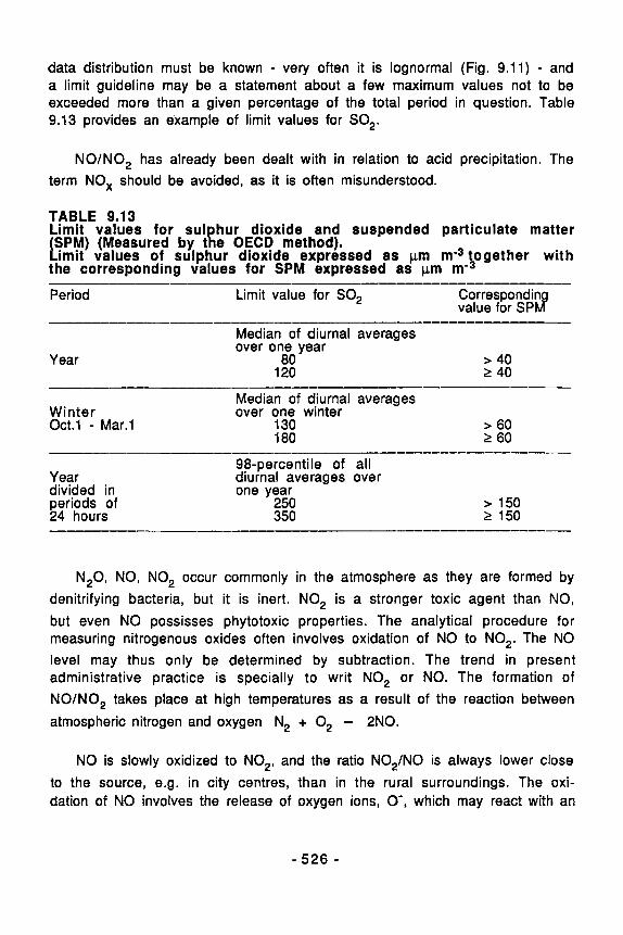
data distribution must be known - very often it is lognormal (Fig. 9.11) - and a limit guideline may be a statement about a few maximum values not to be exceeded more than a given percentage of the total period in question. Table 9.13 provides an example of limit values for SO,.

NO/NO, has already been dealt with in relation to acid precipitation. The term NOx should be avoided, as it is often misunderstood.

TABLE 9.13 Limit values for sul hur dioxide and suspended particulate matter [SPM) (Measured by t\e OECD method).

imit values of sulphur dioxide expressed as pm m-3 together with the corresponding values for SPM expressed as pm mm3

Period Limit value for SO, Correspondin value for S P ~

Median of diurnal averages over one year

Year ao > 40 120 2 40

-- ~

Median of diurnal averages Winter over one winter 0ct.l - Mar.1 130 > 60

180 2 60

98-percentile of all Year diurnal averages over divided in one year periods of 250 > 150

2 150 24 hours 350 ---- ----- ~ -------- ---

N,O, NO, NO, occur commonly in the atmosphere as they are formed by

denitrifying bacteria, but it is inert. NO, is a stronger toxic agent than NO,

but even NO possisses phytotoxic properties. The analytical procedure for measuring nitrogenous oxides often involves oxidation of NO to NO,. The NO

level may thus only be determined by subtraction. The trend in present administrative practice is specially to writ NO, or NO. The formation of

NO/NO, takes place at high temperatures as a result of the reaction between

atmospheric nitrogen and oxygen N, + 0, - 2N0.

NO is slowly oxidized to NO,, and the ratio NO,/NO is always lower close

to the source, e.g. in city centres, than in the rural surroundings. The oxi- dation of NO involves the release of oxygen ions, 0-, which may react with an

- 526 -

oxygen molecule 0, to form 0, (NO + 0, - NO, + 0-; 0- + 0, - 0,).

TABLE 9.14 A photochemical model

1. NO, + hv - NO + 0

NOx 2. O + O , + M - O , + M

cycle 3. 0, + NO - NO, + 0,

produces 4. 0, + NO, - NO, + 0,

5. NO, + NO, 2HNO, nitric acid

6. NO + NO2 2HN02 nitrous acid

H2O

H2O

7. HN02 + hv - NO + OH

CO, + HO, CO roduces 7 an 8 H chain 8. CO + OH

9. HO, + NO - NO, + OH ~ ~~~~~

10. HC + 0 - aRO,*

12. HC + OH - dRO,' + eRCHO peroxy radicals

11. HC + 0, - bRO,* + CRCHO aldehyde and

13. HC + RO, - fRO,* + gRCHO ~ _ _ ~ ~~ ~~~

14. RO, + NO - NO, + hOH oxidation of NO to NO, ~~~~~

15. RO, + NO, - PAN ~~

production of peroxy- acetyl nitrate

_--------__------------- HC = hydrocarbon a - h stoichiometric coefficients RO,' = peroxy radical M = catalyst

Source: Seinfeld, 1971. See also T.A. Hecht adn J.H. Seinfeld, Environ. Sci. Technol. vol. 6, pp. 47-57, 1972; R.G. Lamb and J.H. Seinfeld, Environ. Sci. Technol. vol. 7, pp. 253-261, 1973.

A large number of photochemical reactions may occur (Table 9.14) in the presence of hydrocarbons, which act deirectly and catalytically, resulting in the so-called photochemical complex with 0, and PAN/PPN (see also section

- 5 2 7 -

5.7). So, NO,/NO pollution should not only be considered in isolation, but also as part of the photochemical smog formation, for which nitric oxides are precursors.The measurement of NO, is usually based on chemiluminescence, and may be made with very short averaging times - half an hour generally being pre- ferred. The measurement of 0, is also based on

chemiluminescence and may be done routinely. The analysis of PAN/PPN, however, is more complicated and involves

sophisticated gas chromatographic techniques.

9.4.4. Particulate matter.

Suspended particulate matter (SPM) has been measured for decades in heavily polluted areas of Europe and North America. SPM may be separated in two fractions, smoke and fly ash, both comprising paritcles less than 10 p in aerodynamic diameter and therefore not significantly influenced by gravitational forces. Soot is black, but smoke be a variety of colours depending on the industrial processes involved in its formation. The reflectrometric method of analysing SPM only gives a measure of the soot component + the black smoke fraction. It is preferable simply to weigh the collecting filters before and after the passage of a given volume of air.

The filters may later be analysed for their content of, for example, heavy metals, using AAS (Atomic Absorption Spectrophotometry) or PIXE (Pictum Induced X-ray Emission spectrophotometry). The major soruces of SPM in cities are traffic exhaust and to a lesser extent point sources, like power plants. Car exhausts contain particles of very small (< 0.5 p) size, composed mainly of lead halogenides. Thus a 1:2 mole ratio between Pb and Zn is found close with distance from the source. Only a small proportion less than 1/4 of the total emission of Pb-containing particles is deposited in the vicinity (i 200 m) of highways etc. The remainder is dispersed and contributes to the common rate of ~ 10 mg rn-,y-’ of Pb in Europe, for example.

power plants is characterized by relatively high concentrations of V and Ni, because these metals accumulate in oil deposits, bound to porphyrin systems from the degraded chlorophyll of carbonaceous plants. The presence of such metal oxides in these particles has a catralytic effect on the oxidation of SO, to SO,, resulting in the production of very acidic particles small enough to be

transported deep into the respiratory tract causing health problems. occasionally transported over large areas, is characterized by

a high content of relatively harmless metals, such as Ti, Fe and Mn. Thus, the composition of airborne particles is important when considering emission reduction and immission guidelines.

The composition of small particles emitted from oil-fired

Soil dust,

- 528 -

Sedimentary dust consists of particles larger than 10 p in diameter that remain in the atmosphere only for short periods, i.8. have residence times of less than 1 hour. Air pollution due to these rather large particles is thus restricted to the immediate surroundings of its factory or power plant source. The adverse health effects from sedimentary dust are negligible, as most of the dust does not reach the respiratory tract and if it does, the particles are retained in the nose or mouth. Only toxic, soluble compounds may then enter the bloodstream and result in health problems.

One of the problems of sedimentary dust concerns its light-inhibiting properies when it covers surfaces, such as glass or plants leaves. Very alkaline or acidic dust particles may have a strong corrosive effect. This type of air pollutant is measured using funnels placed in a network around the factory or in a selected investigation area. It is generally not considered a major air pollution problem, as its control is rather simple and effective.

H F/F- are mainly emitted from brick, glass, porcelain and fertilizers factories and the impact on the environment is generally restricted to the immediate neighbourhood of the source.

Fluorides are very soluble in water and thus easily washed off and attached to particles with a surface water film. The emission of fluorides is thus controlled by deposition measurements close to the source. Deposition on plants has led to local cattle fluorosis.

9.4.5. Heavy metals.

When dealing with air pollution due to heavy metals, the complexity of the chemistry of these elements must be borne in mind. Lead provides a good example (see Table 9.15).

P.9.15. The different chemical compounds have different toxic properties and it makes no sense to reduce the immission exclusively on a quantitative basis simply by reducing the level of the most common compounds in the atmos- phere.

Generally, the heavy metals are attached to particles or form particles with a few anions (SO,'-, X-), mercury being an important exception.

Emission and re-emission form soil of gaseous Hg and alkyl-Hg occur, and re-emission probably also occurs to a smaller degree with a few other heavy metals, such as Cd.

Heavy metals immission is determined by filter analysis following passage of a known volume of air through the filter. Separation into particle size groups is often made, e.g. between paricles less than 2.5 p and between

- 5 2 9 -

2.5 and 20 p.

smaller than 2 p. Lead halogenides are confined to small particles, 60-70 per cent being

TABLE 9.15 Lead compounds as airpollutants -_I-------

9.4.6. Hydrocarbons and carbon monoxide.

Hydrocarbons are present in high concentrations in city atmospheres, originating mainly from car exhausts. The complexity of the hydrocarbon im- mission is illostrated in Fig. 9.72. By far the most common hydrocarbon is methane (CH,), which usually constitutes more than 80 per cent of the total

hydrocarbon content of the atmosphere. The hydrocarbons are either formed during combustion, being more or less completely oxidized, or simply evapo- rated into the surrounding air from cars (crank case, carburetor and petrol tank).

P.9.16. The hydrocarbons in city atmosphere represent a rather large health problem, and several are believed to be car- cinogenic.

Due to the complexity of hydrocarbon immission, its control has been limited in most areas; instead, efforts have been concentrated on reducing emission, and cars have been fitted with a veriety of devices to improve their combustion efficiency.

This has also resulted in a reduction in CO emission. Carbon monoxide is frequently measured in city atmosphere because of its potentially hazardous effect of inhibiting the blood's oxygen uptake. Carbon monoxide quickly becomes well dispersed in the air because its relative density is very close to the average air density (28 and 29). It has practically no effect on plants, however, partly because of its very low solubility in water.

- 5 3 0 -

22 -

n-Eutyl k n z e n e

r-nutyl knzene

o-Xylenc

n-0ctme k ? 9 C-l r imr)hul hr-snr

18 - F 16 F f i 14

xim I?

10

M

N 1 0

2.2.4-Trimeth~

c

Toluene

2.3- Dimethyl yk ?.?-Dimethyl butane

- _ Ethane .- 4 c;2B

SINI1C.H VALVE

-1

2r' 0

?== Cyclapentcne

pentane Eeni - iene

> I-Methyl-l-Eutene I IfAm i cis-2-B tew e - z - i u t e n e tadieni n ~ B utane

! - I - utene I-Butene -Propyne Propadiene

Acetylene --p L- Ethane Ethylene

c ropylene

Mefhane

Fig.. 9.12. mobile engine. (Hafstad, 19697.

Gas chromato raph showing products of combustion in auto-

- 5 3 1 -

TABLE 9.16

I /

Averaging P o l l u t a n t time

Photochemical 1 hour oxidants (corrected f o r NO2)

Carbon mon- 12 hours oxide

8 hours

1 hour

Nitrogen ATlnUd dioxide average

California standarde

Concen tra tiang Me thode

0 10 ppm Neutral buffered KI

(;OO pg/m3)

10 ppm Nondispersive (11 mg/m3) infrared

spectroscopy

40 ppm (46 mg/m3)

Saltzman method

10 mg/m3

40 mg/d

100 pg/m3 ( 0 . 0 5 ppm)

( 9 ppm)

(35 ppm)

average

24 hours 0.04 ppm Conductimetric (105 #g/m3) method ! 3 hours

dioxide

Same as Nondispersive primary infrared standards spectroscopy

same as Col 0 r i m e t ri c primary method using standarda NaOH

1 hour

Federal standardsd

primary method standards

0.25 ppm ( 4 7 0 irg/m3)

Suspended particulate m a t t e r

Lead (particulate)

Hydrogen sulphids

Hydrocarbons (oorrected for methane)

Visibility =educing partlclea

1700 ueh3 1

1 hour 0 . 5 ppm (1310 i ig /m3)

Annual 6 0 pg/m3 High volume geometric sampling mean

24 hours 100 &g/m3

30 day 1.6 UJ.3 High volume average sampling.

dithizone method

1 hour 0 . 0 3 ppm Cadmium (42 pg/m3) hydroxide

STRae tan method

3 hours ( 6 - 9 am)

1 obaer- In sufficient amaunt to re- vation duce the prevailing visibility

to 10 miles when the relative humidity is less than 70%

sampling

Flame ionization detection u~ing

Notes: a. Any equivalent procedure which can be shown to the satisfaction of the Air R e s o u r c e s Board to give equivalent results at or near the level Of the air quality standard may be Used.

safety. t o protect the public health. Each state must attain the primary standarde no later than three years af ter that state's implementation plan is approved by the Environmental Protection Agency (EPA).

C . National Secondary Standards: The levels of air quality nece4sary to protect the public w e l l f a r e from any known or anticipated adverse effects o f pollutant. Each state must attain the secondary standards within a 'reasonable time" after implementation plan is approved by the EPA.

d. Federal Standards, other than those based on annual averages or annual geometric means, are not to be exceeded more than once per year.

e . Reference method as described by the EPA. An "equivalent metbod" Of measurement may be used but m u s t have a "consistent relationship to the reference method" to be approved by the EPA.

f . Prevailing visibility 13 defined as the greatest visibility which is attained or surpassed around at least half of the harrzon Circle, but not necessarily in continuous seotora.

g. Concentration expressed first in units In Which it w a s promulgated. Equivalent unite given in parantheses are based upon a reference temperature o f 25OC and a reference pressure of 760 mm of He.

h. Corrected for SO2 in addition to NO2. i. Revoked in 1973.

b. National Primary Standards: The levels Of air quality necessary. with an adequate margin of

- 5 3 2 -

9.4.7. Biological monitoring.

P.9.17. Biological monitoring involves several different app- roaches, but aims always to evaluate the impact of pollutant on living systems by observing changes in the systems themselves after exposure to the immission.

The impact recorded is most often an adverse effect, but may also be the accumulation of heavy metals, for example. The following paragraphs discuss some typical examples of biological monitoring.

Epiphytic lichens have been used to reflect levels of a number of parti- cularly gaseous pollutants, such as SO, and HFIF-. A number of cities in

Europe and North America have been extensively studied with respect to lichen growth on trees. The general pattern is a decrease in the frequency of occurrence of most species with proximity to the city centre, with a few species showing the opposite trend. The correlation between species distribution and levels of SO, is often very good, and a number of laboratory

experiments have shown a causal relationship between SO, levels and lichen

injury/performance; the species sensitivity sequence observed in the laboratory closely follows the field observations.

The presence of suspended particulate matter in the city atmosphere does not in itself contribute significantly to a reduction in lichen growth. On the contrary, the predominance of oxides in the particles may result in an alkaline reaction when suspended in water; the presence of SO,, however,

more than neutralizes this effect, and the lichen substratum, the tree bark, becomes more acidic the closer it is to the city centre. Of course, this effect contributes indirectly to the overall change in population distribution.

In relation to biological monitoring, a number of lichen species can be used as indicators to estimate SO, levels; if a certain species occurs in the

investigation area, the SO, immission cannot exceed the critical value for that species. An example is given in Fig. 9.13 A-E.

Several questions arise when relating species distribution to ambient SO, levels, namely how specific is the reaction: are other pollutants present that may also adversely affect the lichens? The question of SPM has already been discussed, and it may safely be anticipated that the above-mentioned indirect effects of SPM generally correlate closely with SO, immission.

With regard to NO,/NO, these pollutants are known to be much less toxic

to plants in general than SO, and at low levels even beneficial. Hydrogen flu-

oride and fluorides, however, are as or more toxic towards lichens than SO,.

-533 -

A B

D

E

- 534 -

Fig. 9.13. The distribution of the indicator lichen species in the investi ation area. o Sampling station. The species present above 30 cm from t#e ground. 0 The s ecies present only below 30 cm from the ground. (Johnsen and Sarchting, 197%).

In areas, where HF/F- are major components of the immission, a biological index has been developed analogous to the one described for SO,.

Fortunately, however, HFIF’ only play a very minor role in the city atmospheres of Europe and North America. In conclusion, epiphytic lichen distributions may be regarded as an overall reaction to the S02-immission, and so their reflect to SO, levels is fully justified. It must be emphasized,

however, that any biological effect index can never be regarded as being 100 percent specific, unlike physicochemical measurements. Table 9.1 7 outlines the major advantages and disadvantages connected with the two methods.

Transplantation is another method of biological monitoring. This method has the great advantage that the investigator is not concerned with the occurrence of trees when planning the study.

TABLE 9.17 Comparison of biological and physicochemical monitoring

Advan tag es Disadvantages

Biolo ical effects Non-specific, essentially Biological of poylutants in the monitoring actual environment Relation to ambient con-

are recorded centration values compli-

Synergismlantago- nism is detectable

-- _____---- - - - _ _ _ _ - - - ~

cated

Specific No effects recorded Phys icochemical Pollutant concentra- Sy nerg ismlantag on ism monitoring tions are measured not detectable -------- ______------

This means that the injury data resulting from a transplantation experiment are generally easier to subject to statistical analysis, as the uniformity of the stations, their distribution and species composition can be determined beforehand and thus optimized. It is probably in the field of transplantation techniques that biological monitoring is progressing best at present.

Transplantation may comprise very different plant groups, and a few examples are given below:

- 5 3 5 -

1. Epiphytic lichens Hypogymnia physodes has been transplanted to around industrial areas or

into cities in order ot evaluate the average SO, immission (Fig. 9.14). The

plants used have been taken from trees either by cutting out bark discs or using of Abies or Larix species. The injury index is based on the bleaching effect of SO,, which will kill the lichen algal component before the lichen

fungus. Using the method for different periods of time may be complicated by the difference in weather conditions. These differences may interfere strongly with the responese in lichens, and when comparing two time periods precautions have to be taken.

2. Higher plants a. 0,-monitoring

Tobacco plants of the variety Bec W3 in particular are very sensitive to 0,, and when exposed to levels that, in general, would not result in crop

damage, a characteristic pattern of spots may occur on the leaves (Fig. 9.15). These spots are caused by dieback of regions of teh mesophyll adjacent to, and the palisade tissue above, the stomata following diffusion of 0, into the leaf.

Extent of damage t ,/

y = -1.07 + 0.0925 x

Fig. 9.14. The correlation between SO, levels at transplanation sites and the extent of transplant thallus damage. r f 0 at p = 0.01. n = number of coinciding dots.

Recording of the total area of the leaf that has been injured gives a semiquantitative measure of the 0, immission, because the reaction is

rather specific. This method has been used extensively in USA, UK and the

- 536 -

Netherlands. The plants may be grown on waste land or in so-called open-top chambers, the last method giving the most easily compared data, because the stations become more uniform.

Y Fig. 9.15A. Sulphur dioxide injury. Leaf necrosis in dicotyledons occur intercostall , in monocotyledons as. necrotic stripes, particular1 near the tip. Right: yransect of healthy and Injuried leaf part. (Garber, 1964.

Fig. 9.15B. Smog-injur In old leaves the leaf base is injured, in young leaves the ti . Transect: The injury begins in the cells around the stomata (Garber, 1967p.

b. HFIF' Accumulation of fluorides in beaves of higher plants leads to a typical

picture of injury: dead whitish tissue surrounded by black, dead bands (Fig. 9.16); in monocotyledons, the dark bands occur close to the leaf tips.

- 537 -

Gladiolus gandavensis has been used to monitor fluorides, and the degree of damage, e.g. measured as the length of the dead (necrotis) area, correlates well with the deposition of fluorides.

Finally, one biological assessment method, that involves a more sophisticated equipment and a larger time scale, is ecosystem monitoring. The use of whole ecosystems, which are limited in some way, e.g. watersheds and lakes, or form a minor part of large, homogeneous systems have the advantage that accumulation rates may be compared with subtle effects at a very early stage.

a b

Fig. 9.16A. a) Transect section of a Prunus leaf injuried by fluorides. b) Normally developed transect section of a Prunus leaf. (Garber, 1967)

FP. 9.166. Fluoride injury in decotyldons and monocotyledons. Typical leaf e ge and. "tip burn" necrosis. In the leaf transect the tissue destruction is clearly visible. (Garber, 1967)

-538 -

A net of such monitor systems have been developed or are under develop- ment in a few countries and will meet the requirements for long-term surveillance of trends in the environment that at present may seem in- significant; typical examples are heavy metal deposition and the slowly increasing levels of organic pollutants in the atmosphere.

- 5 3 9 -