This article has been accepted for inclusion in a future issue of this journal. Content is final as presented, with the exception of pagination.

IEEE JOURNAL OF SELECTED TOPICS IN APPLIED EARTH OBSERVATIONS AND REMOTE SENSING 1

Evaluation of Ozone Analyses From UARS MLSAssimilation by BASCOE Between 1992 and 1997

S. Viscardy, Q. Errera, Y. Christophe, S. Chabrillat, and J. -C. Lambert

Abstract—We present the analyses of UARS MLS ozone dataobtained by the Belgian Assimilation System for ChemicalObsErvations (BASCOE). This system, based on the 4D-varmethod, is dedicated to the assimilation of stratospheric chemistryobservations. It uses a 3-D Chemical Transport Model (3D-CTM)including 57 chemical species with explicit calculation of strato-spheric chemistry. The CTM is driven by ECMWF ERA-40analyses of winds and temperature, with a horizontal grid of 3.75in latitude by 5 in longitude, and with 37 pressure levels fromthe surface to 0.1 hPa. BASCOE has assimilated UARS MLSobservations acquired during the period 1992–1997. We discusshow BASCOE is able to reproduce MLS data, and we evaluatethe BASCOE analyses with respect to independent observationsfrom UARS HALOE, ozonesondes, and ground-based lidars. Anexcellent agreement is found with independent observations (biasusually less than 10%), except in the lowermost stratosphereand in the Antarctic ozone hole. The performances of BASCOEozone analyses are also compared to those of two other long-termozone reanalyses; namely, ERA-40 and ERA-Interim, both fromECMWF. Finally, sensitivity test based on BASCOE free modelruns suggest that ozone analyses during the ozone hole periodwould be greatly improved by driving BASCOE with the dynam-ical fields of the new ECMWF reanalyses ERA-Interim. This workis part of the Stratospheric Ozone Profile Record service raised bythe GMES Service Element PROMOTE.

Index Terms—BASCOE, 4D-Var assimilation, GMES, ozone,PROMOTE.

I. INTRODUCTION

M ORE than 20 years after the signature of the Montrealprotocol in 1986, understanding the evolution of strato-

spheric ozone during the 21st century and predicting the ozonerecovery is a question of great interest, especially in the contextof climate change. Since ozone strongly interacts with the ra-diation field and with a large number of chemical constituents,making such predictions requires numerical modelling takinginto account dynamical, radiative and chemistry processes andtheir interactions. These Chemistry Climate Models (CCMs)generally start their simulation in the third quarter of the 20thcentury and return predictions for several hundreds of years[13], [14]. Since the predictions can vary significantly between

Manuscript received April 22, 2009; revised September 14, 2009. This workwas supported in part by ProDEx and the Belgian Science Policy Office via theproject SECPEA (C90328) and in part by ESA’s GMES Service Element for theAtmosphere PROMOTE (http://www.gse-promote.org).

The authors are with the Belgian Institute for Space Aeronomy(BIRA-IASB), Belgium.

Color versions of one or more of the 1dures in this paper are available onlineat http://ieeexplore.ieee.org.

Digital Object Identifier 10.1109/JSTARS.2010.2040463

different models, their geophysical validation is a crucial task.One aspect of the validation is to compare CCM simulationsduring the nineties against observations retrieved during thisperiod [12]. Since these observations are asynoptic, i.e., dis-tributed irregularly in space and time, comparison with CCMoutput requires to interpolate model values in the observationspace. Moreover, some key chemical constituents are rarely(or not) observed, like total chlorine in the South Pole polarvortex. Accordingly, 4-D Variational (4D-Var) data assimilationcoupled with a model including explicitly the stratosphericchemistry can provide synoptic analyses of observed chemicalspecies and some of the nonobserved species [11], [22].

In order to support CCM Validations done under the auspicesof SPARC (Stratospheric Process and their Role in Climate), thePROtocol MOniToring (PROMOTE) project (www.gse-pro-mote.org) developed the Stratospheric Ozone Profile Recordservice.1 This service will generate analyses of ozone and othertrace gases from the assimilation of UARS MLS, GOME,MIPAS, and SCIAMACHY covering the period between 1992and the end of the Envisat mission [8]. Within this service,ozone analyses made by assimilation of GOME [8] and MIPAS[10] observations have already been discussed.

UARS MLS observations have already been assimilated forshort time periods, mainly to demonstrate the applicability ofassimilation methods to observations of atmospheric chemistry[19], [23]. A new MLS instrument was launched in 2004onboard the AURA satellite and several groups have reportedon the assimilation of these ozone observations for the year2005 [15], [18], [35]. Here, we present and evaluate a long-termdataset of ozone analyses produced by the assimilation ofUARS MLS observations. The assimilation system is namedBASCOE and the investigated period covers the years 1992 to1997. The evaluation is carried out by an intercomparison withindependent observations (HALOE, ozonesondes and lidars)and two well-known ECMWF assimilation systems (ERA-40and ERA-Interim) that also cover the same period.

The paper is organized as follows: Section II describes theBASCOE system; some features of UARS MLS, independentobservations (HALOE, ozonesondes and lidars) and other as-similation systems are provided in Sections III, IV, and V, re-spectively; Section VI briefly explains the intercomparison pro-cedure used for evaluation; Section VII is dedicated to the re-sults of the evaluation of BASCOE analyses; Section VIII dis-cusses some issues uncovered in the BASCOE analyses; finally,conclusions and perspectives are presented in Section IX.

1Website: http://wdc.dlr.de/data_products/projects/promote/3D-Ozone/pro-mote_3d-ozone.html

1939-1404/$26.00 © 2010 IEEE

Authorized licensed use limited to: Univ of Calif San Diego. Downloaded on April 28,2010 at 12:45:31 UTC from IEEE Xplore. Restrictions apply.

This article has been accepted for inclusion in a future issue of this journal. Content is final as presented, with the exception of pagination.

2 IEEE JOURNAL OF SELECTED TOPICS IN APPLIED EARTH OBSERVATIONS AND REMOTE SENSING

II. BASCOE DESCRIPTION

The Belgian Assimilation System for Chemical ObsErva-tions2 is a 4-D variational (4D-Var) system dedicated to theanalyses and forecast of stratospheric chemical data [10]. Itdescends from Errera and Fonteyn [11]. The 3D-CTM uses foradvection the Flux Form Semi-Lagrangian scheme [24] with atime step of 30 min. Chemical interactions of 57 species are ex-plicitly calculated with 143 gas-phase reactions, 48 photolysisreactions, and nine heterogeneous reactions with parameterizedPSC surface area densities and sedimentation.

The BASCOE model neglects the variation of the sunrise andsunset time in function of the altitude. Its photochemical modelassumes a cutoff of the photodissociation at a solar zenith an-gles of 96 , which is representative of the middle stratosphere( km). In reality, the sun sets 20 min earlier at 10 km,and 12 min later at 60 km. Since these errors are comparableto the model timestep (30 min), the approximation can lead tonon-negligible errors in the lower and upper stratosphere forcomparisons of short-lived species with solar occultation obser-vations. No interannual variation is taken into account by thephotochemical model. In particular, the solar spectrum used tocalculate photolysis coefficients is kept constant at solar min-imum conditions and the total amount of stratospheric chlorineis kept constant at a loading representative of the mid-nineties.

For the present study, the CTM is driven by the ECMWFERA-40 analyses of winds and temperatures [36]. The atmos-phere is discretized on a 5 longitude by 3.75 latitude grid andon a vertical grid consisting in a subset of 37 pressure levels outof the 60 ECMWF set of levels, from 0.1 hPa down to the sur-face. Hence, the horizontal grid resolution corresponds roughlyto maximum 555 km in longitude by 415 km in latitude, and thevertical resolution is close to 1.5 km in the middle stratosphere,1 km at 100 hPa and 1.5 km at 250 hPa.

The assimilation of observations is performed over a timewindow of one day with a background error covariance matrixset diagonal with a standard deviation of 50%. The implicationof a diagonal background error covariance matrix are discussedin Errera et al. [10]. The system also includes a data filter to re-ject observations too far from the BASCOE initial guess: all ob-servations greater than three times, or smaller than one third, ofthe background state are rejected. The BASCOE analyses eval-uated in this paper are labelled MLS_v4q09.

III. MLS DESCRIPTION

The Microwave Limb Sounder (MLS) was one of the teninstruments on board of the UARS satellite launched onSeptember 12, 1991 [2]. It provided multi-year measurementsof stratospheric ozone and related trace gases with a relativelyhigh amount of observations (see Table I). The UARS orbit hada 56 inclination while MLS scanned the atmosphere perpen-dicularly to the orbit. In addition, UARS performed a 180 yawsteering manoeuvre about every 36 days. In consequence, MLSpresented two modes of observation: one directed to the north(latitude: 34 S–80 N) and the other one directed to the south

2Originally, BASCOE was developed to assimilate Envisat data. The acronymthen meant Belgian Assimilation System for Chemical Observations from EN-VISAT.Website : http://www.bascoe.oma.be/promote/bascoe_sys.html

TABLE INUMBER OF DAYS OBSERVED BY UARS MLS PER YEAR BETWEEN 1992 AND

1997. 1317 PROFILES ARE RETRIEVED ON EACH FULL DAY OF OBSERVATIONS

TABLE IIESTIMATED BIAS AND PRECISION OF MLS OZONE FOR DIFFERENT PRESSURE

LEVELS BETWEEN 0.2 HPA AND 100 HPA AS REPORTED BY LIVESEY et al. [25]

(latitude: 80 S–34 N). In this paper, we shall refer to thesetwo UARS observations modes as the North mode and Southmode. In the unobserved latitudes, the BASCOE analyses maybe considered as the output of a free CTM run initialized bythe analysis of the day preceding the yaw steering manoeuvre,except that a little information is brought from observed lat-itudes due to transport. The MLS profiles are provided onthe UARS pressure levels (i.e., six pressure levels per decadewhich corresponds approximately to 2.5 km), and the intervalbetween successive profiles is 495 km.

The primary target chemical species of UARS MLS wereozone (O ), chlorine monoxide (ClO) and water vapor (H O).Nevertheless, the successive retrieval algorithms have alsoprovided profiles of other species such as nitric acid (HNO ),hydrogen peroxide (H O ), sulfur dioxide (SO ), and methylcyanide (CH CN). In the present evaluation, we have used thelatest and most definitive MLS version 5 dataset (Level 3AT)validated by Livesey et al. [25]. While this paper focuses on theozone analyses, all of the MLS species have been assimilatedsimultaneously by BASCOE, except CH CN.

MLS consisted of three radiometers tuned on 63, 183, and205 GHz, respectively. The stratospheric ozone profile, which isthe quantity of interest for BASCOE, was obtained from the lastradiometer (hereafter denoted by O3_205). On July 13, 1997,the 63-GHz radiometer used to retrieve the temperature profilewas switched off in order to save spacecraft power. The retrievedtemperatures used for the O3_205 retrieval were replaced fromthis date onward by temperature analyses produced by NationalCenters for Environmental Prediction (NCEP) or by the UARStemperature climatology where NCEP data were not available.In consequence, the quality of ozone retrievals has been reducedafterwards [25]. In addition, the number of operating days ofMLS (see Table I) has decreased over the years due to technicalreasons [25].

Table II provides the estimated bias and precision of MLSobservations at different pressure levels as evaluated byLivesey et al. [25]. As recommended, ozone profiles are as-similated only in the pressure levels between 0.2 and 100 hPa.Finally, Livesey et al. [25] also recommend to discard the ozone

Authorized licensed use limited to: Univ of Calif San Diego. Downloaded on April 28,2010 at 12:45:31 UTC from IEEE Xplore. Restrictions apply.

This article has been accepted for inclusion in a future issue of this journal. Content is final as presented, with the exception of pagination.

VISCARDY et al.: EVALUATION OF OZONE ANALYSES FROM UARS MLS ASSIMILATION BY BASCOE BETWEEN 1992 AND 1997 3

TABLE IIILIST OF THE 15 NDACC STATIONS WITH OZONESONDES USED IN THIS WORK. ALL THESE OZONESONDES ARE OF ECC-TYPE, EXCEPT THESE IN

HOHENPEISSENBERG (BREWER-MAST) AND IN UCCLE (BREWER-MAST UNTIL 1997; ECC FROM 1997 ONWARDS)

data after 1998 for scientific purposes. Accordingly, we shallconsider only the period 1992–1997 in this paper.

IV. INDEPENDENT OBSERVATIONS

A. UARS HALOE

Halogen Occultation Experiment (HALOE) operated onboard of UARS, together with MLS. The instrument used themethod of solar occultation to retrieve vertical profiles of theabundances of chemical species, one of which being ozone[31]. The precession of UARS associated with its 56 orbitinclination yielded a latitude sampling from 80 S to 80 Nin about one month by performing around 15 sunset and 15sunrise occultations each day. According to Brühl et al. [5]who validated HALOE version 17, random errors are below 5%above 10 hPa and increase up to 11% at 100 hPa. The system-atic errors increase from 5% at 0.4 hPa to 28% at 100 hPa with10% at 10 hPa. Comparison of HALOE version 19, the versionused in this paper, with correlative data shows an agreement ofabout 5% in the stratosphere [4], [28], [30].

Finally, we note that, due to the UARS yaw steering ma-noeuvre, HALOE polar observations are always performed inthe hemisphere opposed to the one observed by MLS. Conse-quently, comparison of Polar BASCOE ozone against HALOEwill always be done in a region where the system is not con-strained by MLS.

B. Ozonesondes

The ozonesondes are used as independent data to evaluateBASCOE analyses from 100 hPa to 10 hPa with a vertical res-olution of a few hundreds meters (up to 250 m). Comparedwith HALOE, they have the advantage to provide observationsover the Pole observed by MLS. Their accuracy is also betterthan HALOE in the lower stratosphere and in the upper tropo-sphere—lower stratosphere (UTLS). Ozonesonde profiles used

in this study are provided by selected NDACC (Network for theDetection of Atmospheric Composition Change [21]) stationsthat cover entirely the period of BASCOE assimilation. Stationnames and coordinates are listed in Table III.

Brewer-Mast (BM) sondes are used at Hohenpeissenberg(whole period) and Uccle (until 1997). Other stations useelectrochemical concentration cells (ECC). The precisionand bias of ECC ozonesondes are, respectively, 3% and 5%between 0 and 20 km (surface—approx. 50 hPa), and 5% and7% between 20 and 35 km (approx. 50 hPa—2 hPa) [34].The mean difference between ozone profiles obtained withboth types of sondes (ECC and BM) is less than 3%, which isfound insignificant with respect to the ECC sonde bias [6]. Inthe following, we shall assume that the different ozonesondedatasets are homogeneous.

Finally, it is known that the quality of the ozone profilesfrom sondes rapidly decreases above 10 hPa. For this reason,ozonesonde data above this level are not used in this paper.

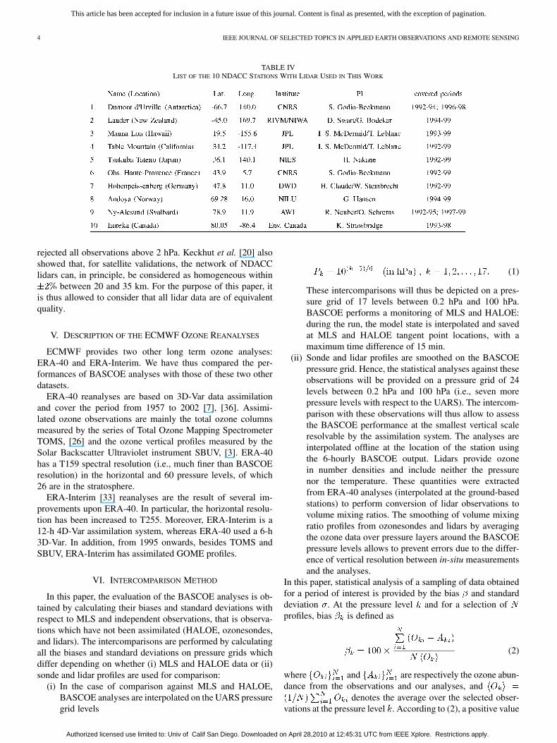
C. Lidar

The last independent datasets used to evaluate BASCOEanalyses are provided by NDACC ozone lidars. Table IV liststhe names and coordinates of these stations that measuredozone during (almost) all the years of the assimilation period.

Typically, lidar instruments measure ozone profiles betweenaltitudes ranging from 8–15 km (approx. 300–120 hPa) to45–50 km (approx. 1 hPa) with a vertical resolution varyingbetween 1 and 4 km from station to station. Keckhut et al. [20]reported that the estimated bias and precision are 2% between20 and 40 km (approx. 100–2 hPa). Above 45 km, the estimatedbias and precision were reported between 5% and 10% but thequality of lidar ozone data becomes largely dependent on themeteorological conditions and instrumental properties. As aconsequence, data quality is unequal from one profile to an-other and from station to station. In this paper, we have simply

Authorized licensed use limited to: Univ of Calif San Diego. Downloaded on April 28,2010 at 12:45:31 UTC from IEEE Xplore. Restrictions apply.

This article has been accepted for inclusion in a future issue of this journal. Content is final as presented, with the exception of pagination.

4 IEEE JOURNAL OF SELECTED TOPICS IN APPLIED EARTH OBSERVATIONS AND REMOTE SENSING

TABLE IVLIST OF THE 10 NDACC STATIONS WITH LIDAR USED IN THIS WORK

rejected all observations above 2 hPa. Keckhut et al. [20] alsoshowed that, for satellite validations, the network of NDACClidars can, in principle, be considered as homogeneous within

between 20 and 35 km. For the purpose of this paper, itis thus allowed to consider that all lidar data are of equivalentquality.

V. DESCRIPTION OF THE ECMWF OZONE REANALYSES

ECMWF provides two other long term ozone analyses:ERA-40 and ERA-Interim. We have thus compared the per-formances of BASCOE analyses with those of these two otherdatasets.

ERA-40 reanalyses are based on 3D-Var data assimilationand cover the period from 1957 to 2002 [7], [36]. Assimi-lated ozone observations are mainly the total ozone columnsmeasured by the series of Total Ozone Mapping SpectrometerTOMS, [26] and the ozone vertical profiles measured by theSolar Backscatter Ultraviolet instrument SBUV, [3]. ERA-40has a T159 spectral resolution (i.e., much finer than BASCOEresolution) in the horizontal and 60 pressure levels, of which26 are in the stratosphere.

ERA-Interim [33] reanalyses are the result of several im-provements upon ERA-40. In particular, the horizontal resolu-tion has been increased to T255. Moreover, ERA-Interim is a12-h 4D-Var assimilation system, whereas ERA-40 used a 6-h3D-Var. In addition, from 1995 onwards, besides TOMS andSBUV, ERA-Interim has assimilated GOME profiles.

VI. INTERCOMPARISON METHOD

In this paper, the evaluation of the BASCOE analyses is ob-tained by calculating their biases and standard deviations withrespect to MLS and independent observations, that is observa-tions which have not been assimilated (HALOE, ozonesondes,and lidars). The intercomparisons are performed by calculatingall the biases and standard deviations on pressure grids whichdiffer depending on whether (i) MLS and HALOE data or (ii)sonde and lidar profiles are used for comparison:

(i) In the case of comparison against MLS and HALOE,BASCOE analyses are interpolated on the UARS pressuregrid levels

(1)

These intercomparisons will thus be depicted on a pres-sure grid of 17 levels between 0.2 hPa and 100 hPa.BASCOE performs a monitoring of MLS and HALOE:during the run, the model state is interpolated and savedat MLS and HALOE tangent point locations, with amaximum time difference of 15 min.

(ii) Sonde and lidar profiles are smoothed on the BASCOEpressure grid. Hence, the statistical analyses against theseobservations will be provided on a pressure grid of 24levels between 0.2 hPa and 100 hPa (i.e., seven morepressure levels with respect to the UARS). The intercom-parison with these observations will thus allow to assessthe BASCOE performance at the smallest vertical scaleresolvable by the assimilation system. The analyses areinterpolated offline at the location of the station usingthe 6-hourly BASCOE output. Lidars provide ozonein number densities and include neither the pressurenor the temperature. These quantities were extractedfrom ERA-40 analyses (interpolated at the ground-basedstations) to perform conversion of lidar observations tovolume mixing ratios. The smoothing of volume mixingratio profiles from ozonesondes and lidars by averagingthe ozone data over pressure layers around the BASCOEpressure levels allows to prevent errors due to the differ-ence of vertical resolution between in-situ measurementsand the analyses.

In this paper, statistical analysis of a sampling of data obtainedfor a period of interest is provided by the bias and standarddeviation . At the pressure level and for a selection ofprofiles, bias is defined as

(2)

where and are respectively the ozone abun-dance from the observations and our analyses, and

denotes the average over the selected obser-vations at the pressure level . According to (2), a positive value

Authorized licensed use limited to: Univ of Calif San Diego. Downloaded on April 28,2010 at 12:45:31 UTC from IEEE Xplore. Restrictions apply.

This article has been accepted for inclusion in a future issue of this journal. Content is final as presented, with the exception of pagination.

VISCARDY et al.: EVALUATION OF OZONE ANALYSES FROM UARS MLS ASSIMILATION BY BASCOE BETWEEN 1992 AND 1997 5

of the bias ( ) indicates that the analyses underestimate theobservations.

Similarly, the standard deviation at the pressure level iswritten as

(3)

Both bias and standard deviation are thus calculated as a per-centage (%) with respect to the observation average .

Over the period 1992–1997, the MLS dataset has many gapsof several days. For these gaps, a BASCOE free model run isperformed. In the comparison between BASCOE and indepen-dent observations discussed later, both BASCOE assimilationand free model run have been considered. In this paper, for itsrepresentativeness, the intercomparisons are mainly carried outfor 1994.

VII. EVALUATION OF THE ANALYSES

A. BASCOE Versus UARS MLS

To check the consistency of the assimilation process,BASCOE analyses have been compared with MLS observa-tions. The qualitative agreement between BASCOE and MLSis summarized in Fig. 1 which shows ozone zonal means over(a) September 1994 and (b) October 1994 for both datasets. InSeptember, the agreement is excellent; the isolines (MLS) andisocontours (BASCOE) are well superimposed. In October, thisis less true in the mid stratosphere southern hemisphere but theagreement remains very good. The difference of agreement be-tween the two months is due to the difference of observed daysfor these two months: while MLS provided observations for al-most every day of September, it was no longer the case for morethan half of October (see http://mls.jpl.nasa.gov/lay/um_calen-dars.html).

In order to get a quantitative estimation of the consistency be-tween BASCOE and MLS, Fig. 2 shows the bias (2) and stan-dard deviation (3) between MLS and our analyses. Statisticshave been calculated over the fall 1994 (from September 1, 1994to November 30, 1994) for five latitude bands. In the middle ofthe stratosphere ( hPa), the bias and standard deviation aresimilar to or less than the estimated bias and precision of MLS asreported by Livesey et al. [25] (see Table II). In the upper strato-sphere ( hPa), the bias is larger but remains small (a fewpercents) whereas the standard deviation grows up to 12%. Inthe mesosphere (0.2–1 hPa), BASCOE overestimation increasesup to 12% in the tropics and the standard deviation up to 50%in high latitudes. In the middle and high latitudes of the lowerstratosphere (100 hPa), the bias and standard deviation remainlower than the estimated bias and precision of MLS. In the trop-ical lower stratosphere, BASCOE is unable to reproduce MLSwithin its uncertainties: the bias and the standard deviation reach40% and 75%, respectively. This is due to the data filter that re-jects more than 65% of the observations. Since this filter usesthe BASCOE initial guess as reference, decreasing the numberof rejected data would require an improvement of the BASCOEmodel in this region. One of the potential improvements would

Fig. 1. Zonal mean of ozone (in ppmv) (a) in September 1994 and (b) in Oc-tober 1994 from BASCOE analyses (isocontours) and MLS observations (iso-lines).

be the introduction in BASCOE of tropospheric processes suchas deep convection and the tropospheric chemistry of ozone.Two other model improvements are discussed in Section VIII,as well as the influence of the yaw steering manoeuvre.

B. Comparison With Independent Observations

1) BASCOE Versus HALOE: In Fig. 2, we also plot biasand standard deviation between BASCOE analyses and HALOEfor fall 1994. Compared to the HALOE error reported in Sec-tion IV-A, the agreement falls within the HALOE uncertaintyexcept (i) in the UTLS, (ii) in the mesosphere, and (iii) at theSouth Pole below 30 hPa during the ozone hole period.

In the UTLS, BASCOE overestimates HALOE by around30% in the middle latitudes and 100% (not shown in Fig. 2)in the tropics. At the same altitude, the standard deviation ofthe differences between HALOE and BASCOE are around 37%and 90% (not shown in Fig. 2) respectively for the same latitudebands. As noted in the comparison with MLS observations, thedegradation of the BASCOE analyses in this region is likely dueto model deficiencies such as the lack of tropospheric processesand other, transport-related issues which are explored in the nextsection.

In the mesosphere, we observe that BASCOE overestimatessignificantly HALOE at 0.3 hPa (depending on the latitude band). However, it was shown by pre-vious studies that ozone observations are not able to constrainozone analyses in that altitude region, both for assimilationsystems that use explicit chemistry modelling [10] and lin-earized chemistry modelling [17]. In the case of BASCOE(which models chemistry explicitly), improving this regionlikely requires to raise the lid of the model in order to improvethe calculation of the photolysis rates, and to take the altitude

Authorized licensed use limited to: Univ of Calif San Diego. Downloaded on April 28,2010 at 12:45:31 UTC from IEEE Xplore. Restrictions apply.

This article has been accepted for inclusion in a future issue of this journal. Content is final as presented, with the exception of pagination.

6 IEEE JOURNAL OF SELECTED TOPICS IN APPLIED EARTH OBSERVATIONS AND REMOTE SENSING

Fig. 2. Comparison between observations and BASCOE analyses between September 1, 1994 and November 30, 1994. These observations are MLS (black line),ozonesondes (red line), lidar (blue line), and HALOE (green line). The grey lines represent the estimated MLS bias (top) and precision (bottom). The range oflatitudes is divided into five bands. The biases � (%) are given in the top row and are calculated using (2). Hence, a positive value of the bias indicates thatthe analyses are lower than the observations. The standard deviations � (%) are in the bottom and are calculated using (3). Between September 1, 1994 andNovember 30, 1994, UARS performed three yaw manoeuvres that divide this period according to the direction of MLS observations (see Section III) as: September1–September 11: South mode; September 13–October 19: North mode; October 21–November 19: South mode; November 22–November 30: North mode (seehttp://mls.jpl.nasa.gov/lay/um_calendars.html).

Fig. 3. Bias and standard deviation (%) between HALOE and BASCOE averaged over each year between 1992 and 1997. The range of latitudes is divided intofive bands. The biases and standard deviation are respectively given in the top and bottom row. According to (2), a positive value of the bias indicates that theanalyses are lower than the observations.

dependent sunrise and sunset time into account (see Section II).On the other hand, the standard deviation of BASCOE againstMLS is higher than against HALOE. This is due to the MLSdata being much less precise in the mesosphere.

At the South Pole, Fig. 2 suggests that BASCOE overesti-mates the ozone field. For example, at 100 hPa(lower stratosphere) and at 0.3 hPa (mesosphere).The BASCOE analyses during ozone hole conditions will bediscussed in detail in Section VII-B2 including comparison ofBASCOE against ozonesondes.

In order to investigate the quality of the BASCOE analysesduring the whole period of MLS assimilation, Fig. 3 shows asuperposition of biases and standard deviations with HALOEdata averaged over each year. Statistics are plotted in the samemanner as in Fig. 2. Generally, bias and standard deviation aresimilar through the period of interest. The only exception is forthe bias above 2 hPa where it decreases from 1992 to 1997 butremains within . This trend in the bias at the uppermostmodel levels may be due to the absence of long-term variationsin the forcings of the BASCOE CTM.

Authorized licensed use limited to: Univ of Calif San Diego. Downloaded on April 28,2010 at 12:45:31 UTC from IEEE Xplore. Restrictions apply.

This article has been accepted for inclusion in a future issue of this journal. Content is final as presented, with the exception of pagination.

VISCARDY et al.: EVALUATION OF OZONE ANALYSES FROM UARS MLS ASSIMILATION BY BASCOE BETWEEN 1992 AND 1997 7

Fig. 4. Illustrations of BASCOE ozone profiles compared to ozonesondes: (a) April 25, 1994 and (b) October 5, 1994 over Amundsen Scott (Antarctica). BASCOEprofiles are plotted in blue. Corresponding ERA-40 and ERA-Interim profiles are also shown in red and green, respectively. Black lines and triangles correspondto ozonesonde profiles and their degradation on BASCOE pressure levels. (b) O3sonde/Am/25–Apr–1994. (b) O3sonde/Am/05–Oct–1994.

2) BASCOE Versus Ozonesondes: Let us first look at in-dividual ozone profiles over the station of Amundsen Scott,in Antarctica. In Fig. 4(a) and (b), we show profiles fromozonesonde observations and BASCOE analyses interpolatedat the location of the station for two dates: April 25, 1994 andOctober 5, 1994. Let us note that MLS was in the North modein both cases. For the first date, the agreement is excellenteven though, around 100 hPa, BASCOE analyses slightlyoverestimate ozonesonde profiles. By contrast, in Fig. 4(b),discrepancies occur between BASCOE and ozonesonde profilesduring the ozone depletion period. Between these two dates,ozone has decreased by around two thirds in BASCOE whileobservations suggest a complete depletion.

The intercomparison between BASCOE analyses andozonesonde measurements is carried out quantitatively throughstatistical analysis by means of bias (2) and standard devi-ation (3) (Fig. 2). In the middle latitudes (60 S-30 S and30 N-60 N) between 20 and 50 hPa, the bias with BASCOEis generally similar ( ) to the estimated bias ofthe sondes themselves (generally, , except below 30 hPain the latitude band [30 N-60 N]) while the standard deviationis greater than the estimated precision ( at 50 hPa).In the tropics at the same levels, bias is positive and slightlylarger ( ) than the ozonesondes estimated bias and thestandard deviation is greater than the estimated precision ofozonesondes ( at 50 hPa). At the North Pole, BASCOEoverestimates the sonde measurements ( ). In the middlestratosphere (between 10 hPa and 30 hPa), the bias is slightlylarger than the estimated bias of the sondes ( ),but it grows in the lower stratophere ( below70 hPa). At the South Pole and at the ozone hole pressurelevels ( hPa), the agreement is much worse (e.g.,

at 100 hPa, not shown in Fig. 2) as expectedfrom Fig. 4(b). In summary, except for ozone hole conditions,a good agreement is found between BASCOE analyses and theozonesondes with a bias usually positive and less than 8% inthe low and middle parts of the stratosphere.

The disagreement above the Antarctic is investigated furtherwith Fig. 5 which shows the time series (data averaged over tendays) of the ozone partial column between 10 and 100 hPa from

BASCOE and the sondes between 1992 and 1997. The ozonehole period is clearly visible in each southern spring where theobserved partial column reaches values between 50 and 100 DUwhile the baseline is around 200 DU. The analysed ozone par-tial column shows a good agreement with the sonde (the rela-tive difference with respect to the observations is less than 10%and mostly positive) for all other seasons. However, during thespring, the ozone hole in BASCOE is not as deep as the obser-vations, differences between the two datasets [Fig. 5(b)] beingaround 50 DU, so that the relative difference increases up to80% with respect to the sondes. The underestimation of polarozone loss by BASCOE has already been discussed in the caseof MIPAS assimilation [10], [16] and is discussed further in thenext section.

Similarly to Fig. 5(a), Fig. 6(a) shows the time series ofthe partial column between 10 and 100 hPa of the sondes andBASCOE at Hohenpeissenberg, where a difference less than 10DU (5% with respect to the observations) and mostly positiveis obtained for most dates before January 1995. From 1995in Hohenpeissenberg, the differences [Fig. 6(b)] increase withtime up to 35 DU (the relative difference reaches 15%). Asmentioned already in Section VII-B1, this increasing overesti-mation is likely due to the decrease in occurrence of the MLSobservations over the years.

3) BASCOE Versus Lidar: Fig. 7(c) and (d) shows lidarozone profiles at, respectively, Mauna Loa (Hawaii) on April15, 1994, and Hohenpeissenberg (Germany) on November 4,1994. These figures illustrate that BASCOE globally yieldsprofiles in good agreement with lidar in the tropical andmid-latitude zones.

The blue lines on Fig. 2 show biases and standard deviationsbetween lidar profiles and BASCOE analyses. In the middle lati-tude bands (60 S-30 S and 30 N-60 N), between 5 and 40 hPa,

, so that the bias is similar to or slightly largerthan the lidar estimated bias (see Section IV-C). The standarddeviation is similar to the lidar estimated precision, except inthe northern middle latitudes where . Below40 hPa, the bias grows and reaches at 100 hPa, while

at 80 hPa in the northern middle latitudes. In thetropics, between 3 and 10 hPa, the bias is usually positive and

Authorized licensed use limited to: Univ of Calif San Diego. Downloaded on April 28,2010 at 12:45:31 UTC from IEEE Xplore. Restrictions apply.

This article has been accepted for inclusion in a future issue of this journal. Content is final as presented, with the exception of pagination.

8 IEEE JOURNAL OF SELECTED TOPICS IN APPLIED EARTH OBSERVATIONS AND REMOTE SENSING

Fig. 5. Time series of ozone partial column (in Dobson units, DU) between 10 and 100 hPa above Amundsen Scott, Antarctica. In the top figure, the black linecorresponds to ozonesonde observations whereas the blue, red and green lines correspond respectively to BASCOE, ERA-40 and ERA-Interim analyses. Thebottom figure displays the difference of ozone partial columns from BASCOE (blue), ERA-40 (red), and ERA-Interim (green) with respect to the sonde.

similar ( ) to the lidar estimated bias. By con-trast, the standard deviation ( ) is larger than thelidar estimated precision. Outside of this range of pressure, biasand standard deviation increase: at 15 Pa, we found respectively

and . The large disagreement in the South Polelatitude band [90 S-60 S] is due to the fact that there is onlyone lidar station in the Antarctic: Dumont d’Urville, which isfrequently located at the vortex edge, i.e., in the most difficultregion for the model.

C. Comparison With ERA-40 and ERA-Interim

In the previous sections, BASCOE ozone analyses has beencompared to observations. Long-term ozone analyses ERA-40and ERA-Interim, generated by ECMWF, give the opportunityto compare the performance of BASCOE (driven by ERA-40analyses of winds and temperature) against well-establishedreanalyses. Figs. 4 and 7 also include ozone profiles fromERA-40 (red line) and ERA-Interim (green line) analyses. Onthese figures, we remark that the three assimilation systemsyield quite different analyses in the middle and upper partsof the stratosphere. Outside of the ozone depletion period(around September 15, 1994 to November 1, 1994), BASCOEis in better agreement with observations than the ECMWFsystems [Figs. 4(a) and 7(a) and (b)]. For example, ECMWFreanalyses underestimate the ozone peak by more than 10%at the tropics, as reported by Oikonomou and O’Neill [29]. Atmiddle latitudes, Fig. 6(b) suggests that the three reanalyses aresimilar until 1997.

During the ozone depletion period [Fig. 4(b)], the linearizedchemistry scheme of ECMWF removes almost all ozone inERA-40 and ERA-Interim in the lower stratosphere. Fig. 5shows that ERA-40 lower stratospheric ozone is in good agree-ment with the ozonesonde at Amundsen Scott, except in Fall1997. On the other hand, ERA-Interim shows periods of pooragreement with sondes despite its improved setup with respectto ERA-40 (see Section V).

VIII. DISCUSSION

Two issues are discussed to assess some of the discrepanciesbetween the BASCOE analyses and independent observations.The first one deals with the impact of the dynamical fields usedto drive the BASCOE CTM, and with its horizontal resolution.The second issue concerns the influence of the MLS viewingmodes on the BASCOE analyses during the ozone hole period.

A. Impact of the Dynamical Fields and of the HorizontalResolution

ECMWF designed the ERA-Interim reanalyses (see Sec-tion V) to address some deficiencies seen in ERA-40 [33]. Ofspecial importance here is the fact that the ERA-40 dynamicalfields deliver a significantly overestimated strength of theBrewer-Dobson circulation [37]. Another source of concern forthe long-term BASCOE re-analysis presented here is its coarsehorizontal resolution (5 3.75 ) imposed by the heavy com-puting cost of the 4D-VAR method. Errera et al. [10] suggestedtwo implications: (i) averaging ERA-40 temperature onto theBASCOE grid inside the polar vortex, especially along its edge,could reduce the occurrence of temperature values below thePSC formation threshold and thus limit the strength of chlorineactivation; (ii) an underestimation of the strong dynamicalbarrier at the vortex edge, allowing mid-latitude ozone to enterthe vortex and reduce the depth of the ozone hole.

These issues were addressed through the execution of threeCTM simulations (Free Model Runs, i.e., with no assimilation)besides the assimilation run evaluated in this paper and labelledMLS_v4q09. These CTM simulations were run for the year1994 and were all initialized from the MLS_v4q09 analysisof January 1, 1994. Their configurations are summarized inTable V. The first CTM experiment, labelled FMR 1, has thesame set-up as the assimilation cycle, i.e., it is run on the samegrid and driven by ERA-40 dynamical fields; the second CTMexperiment (FMR 2) is also run on the same grid but it is driven

Authorized licensed use limited to: Univ of Calif San Diego. Downloaded on April 28,2010 at 12:45:31 UTC from IEEE Xplore. Restrictions apply.

This article has been accepted for inclusion in a future issue of this journal. Content is final as presented, with the exception of pagination.

VISCARDY et al.: EVALUATION OF OZONE ANALYSES FROM UARS MLS ASSIMILATION BY BASCOE BETWEEN 1992 AND 1997 9

Fig. 6. Same as Fig. 5 but for ozonesondes released from Hohenpeissenberg, Germany.

Fig. 7. Illustrations of BASCOE ozone profiles compared to lidar data. Lidar data are on (a) April 15, 1994 over Mauna Loa (Hawaii) and on (b) November 4,1994 over Hohenpeissenberg (Germany). BASCOE profiles are plotted in blue. Corresponding ERA-40 and ERA-Interim profiles are also shown in red and green,respectively. Black lines and triangles correspond to lidar profiles and their degradation on BASCOE pressure levels. (a) Lidar/Ml/15–Apr–1994. (b) Lidar/Ho/21–Oct–1994.

TABLE VLIST OF THE DIFFERENT BASCOE RUNS AND THEIR CHARACTERISTICS. THE FIRST COLUMN PROVIDES THE LABELS OF THESE RUNS. THE SECOND ONE

INDICATES WETHER THESE HAVE ASSIMILATED MLS OR ARE FREE MODEL RUNS. THE LAST TWO COLUMNS GIVE THEIR RESPECTIVE HORIZONTAL RESOLUTION

AND THE DRIVING WIND FIELDS

by ERA-Interim dynamical fields; the last CTM experiment(FMR 3) is run with a finer horizontal resolution (3.75 2.5 )and is driven by ERA-Interim dynamical fields.

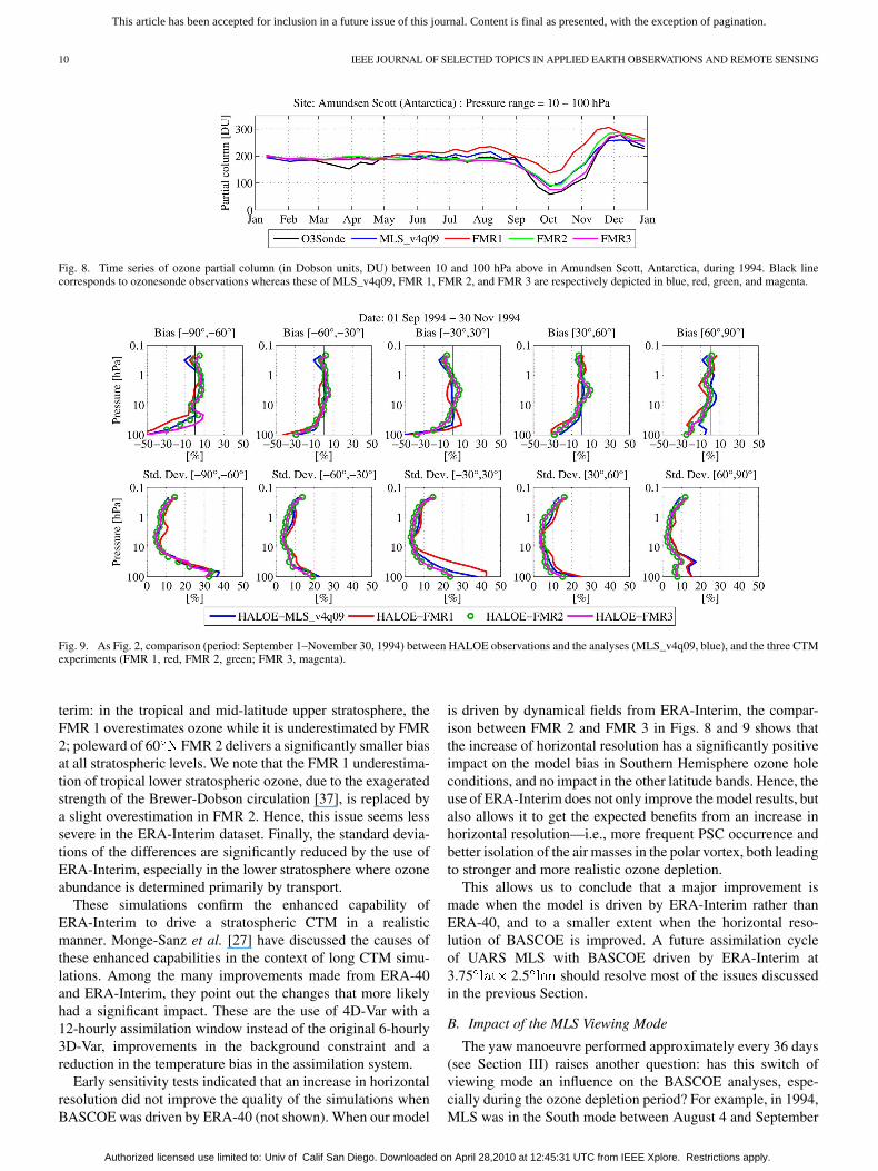
Comparing FMR 1 and FMR 2 allows us to evaluate the im-pact of ERA-40 on the model and the potential improvementsthat can be done using ERA-Interim. Fig. 8 presents the evolu-tion of the partial columns between 10 to 100 hPa for 1994 forthe ozonesondes, the BASCOE analyses and CTM free modelruns. It shows that the CTM driven by ERA-40 (FMR 1) seri-

ously underestimates ozone depletion. This underestimation ispartly corrected by the assimilation of MLS observations, andcorrected to the same extent by driving the CTM with ERA-In-terim (FMR 2). This important result is confirmed by the biasesbetween these simulations and HALOE observations, as shownby the upper-left plot of Fig. 9 which shows the statistical eval-uation of these CTM experiments and of the analyses, usingHALOE as a reference. In the other latitude bands, the bias isalso significantly modified when the CTM is driven by ERA-In-

Authorized licensed use limited to: Univ of Calif San Diego. Downloaded on April 28,2010 at 12:45:31 UTC from IEEE Xplore. Restrictions apply.

This article has been accepted for inclusion in a future issue of this journal. Content is final as presented, with the exception of pagination.

10 IEEE JOURNAL OF SELECTED TOPICS IN APPLIED EARTH OBSERVATIONS AND REMOTE SENSING

Fig. 8. Time series of ozone partial column (in Dobson units, DU) between 10 and 100 hPa above in Amundsen Scott, Antarctica, during 1994. Black linecorresponds to ozonesonde observations whereas these of MLS_v4q09, FMR 1, FMR 2, and FMR 3 are respectively depicted in blue, red, green, and magenta.

Fig. 9. As Fig. 2, comparison (period: September 1–November 30, 1994) between HALOE observations and the analyses (MLS_v4q09, blue), and the three CTMexperiments (FMR 1, red, FMR 2, green; FMR 3, magenta).

terim: in the tropical and mid-latitude upper stratosphere, theFMR 1 overestimates ozone while it is underestimated by FMR2; poleward of 60 FMR 2 delivers a significantly smaller biasat all stratospheric levels. We note that the FMR 1 underestima-tion of tropical lower stratospheric ozone, due to the exageratedstrength of the Brewer-Dobson circulation [37], is replaced bya slight overestimation in FMR 2. Hence, this issue seems lesssevere in the ERA-Interim dataset. Finally, the standard devia-tions of the differences are significantly reduced by the use ofERA-Interim, especially in the lower stratosphere where ozoneabundance is determined primarily by transport.

These simulations confirm the enhanced capability ofERA-Interim to drive a stratospheric CTM in a realisticmanner. Monge-Sanz et al. [27] have discussed the causes ofthese enhanced capabilities in the context of long CTM simu-lations. Among the many improvements made from ERA-40and ERA-Interim, they point out the changes that more likelyhad a significant impact. These are the use of 4D-Var with a12-hourly assimilation window instead of the original 6-hourly3D-Var, improvements in the background constraint and areduction in the temperature bias in the assimilation system.

Early sensitivity tests indicated that an increase in horizontalresolution did not improve the quality of the simulations whenBASCOE was driven by ERA-40 (not shown). When our model

is driven by dynamical fields from ERA-Interim, the compar-ison between FMR 2 and FMR 3 in Figs. 8 and 9 shows thatthe increase of horizontal resolution has a significantly positiveimpact on the model bias in Southern Hemisphere ozone holeconditions, and no impact in the other latitude bands. Hence, theuse of ERA-Interim does not only improve the model results, butalso allows it to get the expected benefits from an increase inhorizontal resolution—i.e., more frequent PSC occurrence andbetter isolation of the air masses in the polar vortex, both leadingto stronger and more realistic ozone depletion.

This allows us to conclude that a major improvement ismade when the model is driven by ERA-Interim rather thanERA-40, and to a smaller extent when the horizontal reso-lution of BASCOE is improved. A future assimilation cycleof UARS MLS with BASCOE driven by ERA-Interim at3.75 2.5 should resolve most of the issues discussedin the previous Section.

B. Impact of the MLS Viewing Mode

The yaw manoeuvre performed approximately every 36 days(see Section III) raises another question: has this switch ofviewing mode an influence on the BASCOE analyses, espe-cially during the ozone depletion period? For example, in 1994,MLS was in the South mode between August 4 and September

Authorized licensed use limited to: Univ of Calif San Diego. Downloaded on April 28,2010 at 12:45:31 UTC from IEEE Xplore. Restrictions apply.

This article has been accepted for inclusion in a future issue of this journal. Content is final as presented, with the exception of pagination.

VISCARDY et al.: EVALUATION OF OZONE ANALYSES FROM UARS MLS ASSIMILATION BY BASCOE BETWEEN 1992 AND 1997 11

Fig. 10. Histograms of the differences between ozonesondes and BASCOE (MLS_v4q09) above Antarctica in the case of (a) MLS South mode and (b) MLSNorth mode. Data from Amundsen Scott, Mac Murdo and Neumayer and during the month September to November of years 1992–1997 have been considered.

12, then in North mode until October 20 when the instrumentis switched back to the South mode. Fig. 8 shows that thistemporary absence of observations has no instantaneous impacton the analyses: there is no discontinuity in the time series ofpartial columns delivered by BASCOE at the end of October,when MLS switches to the South viewing mode.

It is still possible to show the impact of the MLS viewingmode in the analyses, at least during ozone hole conditions whenthe observations have a large impact on the analyses. Fig. 10shows the histogram (distribution of occurrences) of the differ-ences between the 10–100 hPa ozone partial columns observedby the ozonesondes and computed from the BASCOE analyses,but considering separately the days of MLS South mode andMLS North mode. These two samples include all soundings re-alized during the months of September, October, and November1992 to 1997 from the stations well inside the Antarctic vortex,i.e., Amundsen Scott, Mac Murdo and Neumayer. We see thatBASCOE is clearly closer to the ozonesonde data when MLS isin the South mode, even though the analyses still underestimateozone depletion by around 24 DU on average.

The persistence of the bias in South mode is due to ourdata filter (see Section II). MLS is generally switching to theNorth mode in mid September, during the development of theozone hole. After the yaw manoeuvre (generally performed onmid-October), the BASCOE state is so far away from the MLSdata that around 55% of the observations are rejected by thedata filter in the 90 S-60 S latitude band. While data filteringis required to allow convergence of the optimization algorithmin the BASCOE system, a simple relaxation of the filteringcriteria may alleviate the issue described here. A more robustsolution lies in model improvements such as those proposedin Section VIII-A. They will improve the background stateof BASCOE, allowing it to accept most of the data currentlyrejected by the system.

IX. CONCLUSION

This paper reports on the evaluation of ozone analyses fromthe assimilation of UARS MLS by the Belgian AssimilationSystem for Chemical ObsErvations (BASCOE) between 1992and 1997. These analyses are produced in the framework of theGMES Service Element PROMOTE within the Stratospheric3-D Ozone Profiles Record service, which is devoted to long-term assimilation of ozone.

The evaluation has included checking the consistency be-tween MLS and BASCOE and comparing BASCOE against in-dependent observations (HALOE, ozonesonde and lidars). Gen-erally, BASCOE reproduces all these datasets within their errorbars, except (i) above 1 hPa, (ii) at the tropical tropopause, and(iii) at the South Pole between 30 and 100 hPa during the ozonehole period. Above 1 hPa, ozone observations are not able toconstrain sufficiently the BASCOE ozone field. Raising the lidof the model and taking into account the altitude dependence ofthe sunrise and sunset time might improve the photochemistryin this region. The disagreement at the tropical tropopause andthe underestimation of polar ozone depletion can be explainedby several causes related to model transport (use of ERA-40 dy-namical fields and horizontal resolution) and to the data filterused in the assimilation procedure. Sensitivity tests based onBASCOE free model runs using ERA-40 and ERA-Interim sug-gest that driving BASCOE with ERA-Interim and twice moregridpoints would greatly improve the BASCOE analyses. A re-laxed data filter will also improve the constraint by the MLS ob-servations, especially during the few days following the switchin the viewing mode. As a matter of fact, this re-analyses workis now part of the EU project MACC. In this framework, theUARS MLS data will be assimilated again using a better datafilter and ERA-Interim to drive BASCOE.

In this paper, the performances of BASCOE have also beencompared to those of two other long-term ozone reanalyses,namely ERA-40 and ERA-Interim, both produced at ECMWF.At the South Pole, ERA-40 is generally in better agreement with

Authorized licensed use limited to: Univ of Calif San Diego. Downloaded on April 28,2010 at 12:45:31 UTC from IEEE Xplore. Restrictions apply.

This article has been accepted for inclusion in a future issue of this journal. Content is final as presented, with the exception of pagination.

12 IEEE JOURNAL OF SELECTED TOPICS IN APPLIED EARTH OBSERVATIONS AND REMOTE SENSING

ozonesondes than BASCOE in the lower stratosphere. In theother regions, BASCOE ozone is closer to independent data thanERA-40. In the case of ERA-Interim, the ozone analyses aboveAmundsen Scott are found poorer than ERA-40 and BASCOE.In summary, except that ERA-40 produces a deeper ozone hole,this work suggests that a more extensive investigation wouldshow that BASCOE analyses are generally more accurate thanECMWF products.

BASCOE ozone analyses can be downloaded from the fol-lowing website: http://www.bascoe.oma.be/promote.

ACKNOWLEDGMENT

The authors would like to thank the European Centre forMedium-Range Weather Forecasts (ECMWF) and the HALOEand MLS Science and Processing Teams at NASA/LaRCand JPL for providing, respectively, meteorological analysesand satellite observations which were used in this work.The ozonesonde and lidar data were obtained as part ofthe Network for the Detection of Atmospheric Compo-sition Change (NDACC) and are publicly available (seehttp://www.ndacc.org). The authors would also like to thankPI institutes listed in Tables III and IV and the staff at thestations for their long-term dedication to lidar and radiosondeactivities, as well as H. De Backer (RMI), S. Godin-Beekmann(CNRS/SA), T. Leblanc (JPL/NASA), W. Steinbrecht (DWD),R. Stuebi (MCH) and many other members of the NDACClidar and ozonesonde working groups for fruitful discussions.

REFERENCES

[1] F. Baier, T. Erbertseder, O. Morgenstern, M. Bittner, and G. Brasseur,“Assimilation of MIPAS observations using a three-dimensionalglobal chemistry-transport model,” Q. J. R. Meteorol. Soc., vol. 131,pp. 3529–3542, 2005.

[2] F. T. Barath, M. C. Chavez, R. E. Cofield, D. A. Flower, M. A. Fr-erking, M. B. Gram, W. M. Harris, J. R. Holden, R. F. Jarnot, and W.G. Kloezeman, “The upper atmosphere research satellite microwavelimb sounder instrument,” J. Geophys. Res., vol. 98, pp. 10751–10762,1993.

[3] P. K. Bhartia, R. D. McPeters, C. L. Mateer, L. E. Flynn, and C. Welle-meyer, “Algorithm for the estimation of vertical ozone profiles fromthe backscattered ultraviolet technique,” J. Geophys. Res., vol. 101, pp.18793–18806, 1996.

[4] P. P. Bhatt, E. E. Remsberg, L. L. Gordley, J. M. McInerney, V. G.Brackett, and J. M. Russell, III, “An evaluation of the quality of halogenoccultation experiment ozone profiles in the lower stratosphere,” J.Geophys. Res., vol. 104, pp. 9261–9276, 1999.

[5] C. Brühl, S. R. Drayson, J. M. Russell, P. J. Crutzen, J. M. McInerney,P. N. Purcell, H. Claude, H. Gernandt, T. J. McGee, I. S. McDermid,and M. R. Gunson, “Halogen occultation experiment ozone channelvalidation,” J. Geophys. Res., vol. 101, pp. 10217–10240, 1996.

[6] H. De Backer, D. De Muer, and G. De Sadelaer, “Comparison of ozoneprofiles obtained with Brewer-Mast and Z-ECC sensors during simul-taneous ascents,” J. Geophys. Res., vol. 103, pp. 19641–19648, 1998.

[7] A. Dethof and E. V. Hólm, “Ozone assimilation in the ERA-40 reanal-ysis project,” Q. J. R. Meteorol. Soc., vol. 130, pp. 2851–2872, 2004.

[8] T. Erbertseder, F. Baier, Q. Errera, S. Viscardy, J. Schwinger, and H.Elbern, “The promote ozone profile service—long-term 3D ozone re-analysis of ERS-2 and Envisat data sets,” presented at the ESA SpecialPublication SP-636: Envisat Symp., 2007.

[9] Q. Errera, S. Bonjean, S. Chabrillat, F. Daerden, and S. Viscardy,“BASCOE assimilation of ozone and nitrogen dioxide observed byMIPAS and GOMOS: Comparison between the two sets of analyses,”presented at the ESA Special Publication SP-636: Envisat Symp.,2007.

[10] Q. Errera, F. Daerden, S. Chabrillat, J. C. Lambert, W. A. Lahoz, S.Viscardy, S. Bonjean, and D. Fonteyn, “4D-Var assimilation of MIPASchemical observations: Ozone and nitrogen dioxide analyses,” Atmos.Chem. Phys., vol. 8, no. 20, pp. 6169–6187, 2008.

[11] Q. Errera and D. Fonteyn, “Four-dimensional variational chemical as-similation of CRISTA stratospheric measurements,” J. Geophys. Res.,vol. 106, no. D13, pp. 12253–12265, 2001.

[12] V. Eyring, N. Butchart, D. W. Waugh, H. Akiyoshi, J. Austin, S. Bekki,G. E. Bodeker, B. A. Boville, C. Brühl, M. P. Chipperfield, E. Cordero,M. Dameris, M. Deushi, V. E. Fioletov, S. M. Frith, R. R. Garcia, A.Gettelman, M. A. Giorgetta, V. Grewe, L. Jourdain, D. E. Kinnison,E. Mancini, E. Manzini, M. Marchand, D. R. Marsh, T. Nagashima,P. A. Newman, J. E. Nielsen, S. Pawson, G. Pitari, D. A. Plummer,E. Rozanov, M. Schraner, T. G. Shepherd, K. Shibata, R. S. Stolarski,H. Struthers, W. Tian, and M. Yoshiki, “Assessment of temperature,trace species, and ozone in chemistry-climate model simulations of therecent past,” J. Geophys. Res., vol. 111, p. D22308, 2006.

[13] V. Eyring, D. E. Kinnison, and T. G. Shepherd, “Overview of plannedcoupled chemistry-climate simulations to support upcoming ozone andclimate assessments,” SPARC Newslett., vol. 25, pp. 11–17, 2005.

[14] V. Eyring, D. W. Waugh, G. E. Bodeker, E. Cordero, H. Akiyoshi,J. Austin, S. R. Beagley, B. A. Boville, P. Braesicke, C. Brühl, N.Butchart, M. P. Chipperfield, M. Dameris, R. Deckert, M. Deushi, S.M. Frith, R. R. Garcia, A. Gettelman, M. A. Giorgetta, D. E. Kinnison,E. Mancini, E. Manzini, D. R. Marsh, S. Matthes, T. Nagashima, P.A. Newman, J. E. Nielsen, S. Pawson, G. Pitari, D. A. Plummer, E.Rozanov, M. Schraner, J. F. Scinocca, K. Semeniuk, T. G. Shepherd,K. Shibata, B. Steil, R. S. Stolarski, W. Tian, and M. Yoshiki, “Multi-model projections of stratospheric ozone in the 21st century,” J. Geo-phys. Res., vol. 112, p. D16303, 2007.

[15] L. Feng, R. Brugge, E. V. Hólm, R. S. Harwood, A. O’Neill, M. J.Filipiak, L. Froidevaux, and N. Livesey, “Four-dimensional variationalassimilation of ozone profiles from the Microwave Limb Sounder onthe Aura satellite,” J. Geophys. Res., vol. 113, p. D15S07, 2008.

[16] A. J. Geer, W. A. Lahoz, S. Bekki, N. Bormann, Q. Errera, H. J. Eskes,D. Fonteyn, D. R. Jackson, M. N. Juckes, S. Massart, V.-H. Peuch,S. Rharmili, and A. Segers, “The ASSET intercomparison of ozoneanalyses: Method and first results,” Atmos. Chem. Phys., vol. 6, no. 12,pp. 5445–5474, 2006.

[17] A. J. Geer, W. A. Lahoz, D. R. Jackson, D. Cariolle, and J. P. McCor-mack, “Evaluation of linear ozone photochemistry parametrizations ina stratosphere-troposphere data assimilation system,” Atmos. Chem.Phys., vol. 7, no. 3, pp. 939–959, 2007.

[18] D. R. Jackson, “Assimilation of EOS MLS ozone observations in theMet Office data-assimilation system,” Q. J. R. Meteorol. Soc., vol. 133,pp. 1771–1788, 2007.

[19] B. V. Khattatov, J. C. Gille, L. V. Lyjak, G. P. Brasseur, V. L. Dvortsov,A. E. Roche, and J. Waters, “Assimilation of photochemically activespecies and a case analysis of UARS data,” J. Geophys. Res., vol. 104,pp. 18,715–18,737, 1999.

[20] P. Keckhut, S. McDermid, D. Swart, T. McGee, S. Godin-Beekmann,A. Adriani, J. Barnes, J. Baray, H. Bencherif, H. Claude, and J.Thayer, “Review of ozone and temperature lidar validations performedwithin the framework of the network for the detection of stratosphericchange,” J. Environ. Monit., vol. 6, pp. 721–733, 2004.

[21] M. Kurylo and R. J. Zandler, “The NDSC—Its status after ten years ofoperation,” in Proc. Quadrennial Ozone Symp., Sapporo, Japan, 2001,pp. 167–168.

[22] W. A. Lahoz, Q. Errera, R. Swinbank, and D. Fonteyn, “Data assimila-tion of stratospheric constituents: A review,” Atmos. Chem. Phys., vol.7, no. 22, pp. 5745–5773, 2007.

[23] P. F. Levelt, B. V. Khattatov, J. C. Gille, G. P. Brasseur, X. X. Tie,and J. W. Waters, “Assimilation of MLS ozone measurements in theglobal three dimensional chemistry transport model ROSE,” Geophys.Res. Lett., vol. 25, no. 24, pp. 4493–4496, 1998.

[24] S.-J. Lin and R. B. Rood, “Multidimensional flux-form semi-la-grangian transport schemes,” Mon. Wea. Rev., vol. 124, pp. 2046–2070,1996.

[25] N. J. Livesey, W. G. Read, L. Froidevaux, J. W. Waters, M. L. Santee,H. C. Pumphrey, D. L. Wu, Z. Shippony, and R. F. Jarnot, “The UARSmicrowave limb Sounder version 5 data set: Theory, characterization,and validation,” J. Geophys. Res., vol. 108, p. D4378, 2003.

[26] R. D. McPeters, P. K. Bhartia, A. J. Krueger, J. R. Herman, B. M.Schlesinger, C. G. Wellemeyer, C. J. Seftor, T. Swissler, O. Torres, G.Labow, W. Byerly, and R. P. Cebula, “Nimbus-7 total ozone mappingspectrometer (TOMS) data products user’s guide,” NASA Ref. Pub., p.1384, 1996.

[27] B. M. Monge-Sanz, M. P. Chipperfield, A. J. Simmons, and S. M. Up-pala, “Mean age of air and transport in a CTM: Comparison of differentECMWF analyses,” Geophys. Res. Lett., vol. 34, p. L04801, 2007.

Authorized licensed use limited to: Univ of Calif San Diego. Downloaded on April 28,2010 at 12:45:31 UTC from IEEE Xplore. Restrictions apply.

This article has been accepted for inclusion in a future issue of this journal. Content is final as presented, with the exception of pagination.

VISCARDY et al.: EVALUATION OF OZONE ANALYSES FROM UARS MLS ASSIMILATION BY BASCOE BETWEEN 1992 AND 1997 13

[28] H. Nazaryan, M. McCormick, and J. Russell, III, “New studies ofSAGE II and HALOE ozone profile and long-term change compar-isons,” J. Geophys. Res, vol. 110, p. D09305, 2005.

[29] E. K. Oikonomou and A. O’Neill, “Evaluation of ozone and watervapor fields from the ECMWF reanalysis ERA-40 during 1991–1999 incomparison with UARS satellite and MOZAIC aircraft observations,”J. Geophys. Res., vol. 111, p. D14109, 2006.

[30] C. E. Randall, D. W. Rusch, R. M. Bevilacqua, K. W. Hoppel, J. D.Lumpe, E. Shettle, E. Thompson, L. Deaver, J. Zawodny, E. Kyrö, B.Johnson, H. Kelder, V. M. Dorokhov, G. König-Langlo, and M. Gil,“Validation of POAM III ozone: Comparisons with ozonesonde andsatellite data,” J. Geophys. Res., vol. 108, p. D4367, 2003.

[31] J. M. Russell, III, L. L. Gordley, J. H. Park, S. R. Drayson, D. H. Hes-keth, R. J. Cicerone, A. F. Tuck, J. E. Frederick, J. E. Harries, and P. J.Crutzen, “The halogen occultation experiment,” J. Geophys. Res., vol.98, pp. 10777–10797, 1993.

[32] J. Schwinger, H. Elbern, and R. Botchorishvili, “A new 4-dimensionalvariational assimilation system applied to Envisat MIPAS observa-tions,” presented at the ESA Special Publication SP-572: Envisat &ERS Symp., Salzburg, 2004.

[33] A. Simmons, S. Uppala, D. Dee, and S. Kobayashi, “ERA-Interim:New ECMWF reanalysis products from 1989 onwards,” ECMWFNewsletter, vol. 110, pp. 25–36, 2007.

[34] H. G. J. Smit, W. Straeter, B. J. Johnson, S. J. Oltmans, J. Davies, D.W. Tarasick, B. Hoegger, R. Stubi, F. J. Schmidlin, T. Northam, A.M. Thompson, J. C. Witte, I. Boyd, and F. Posny, “Assessment of theperformance of ECC-ozonesondes under quasi-flight conditions in theenvironmental simulation chamber: Insights from the Juelich OzoneSonde Intercomparison Experiment (JOSIE),” J. Geophys. Res., vol.112, p. D19306, 2007.

[35] I. Stajner et al., “Assimilated ozone from EOS-Aura: Evaluation of thetropopause region and tropospheric columns,” J. Geophys. Res., vol.113, p. D16S32, 2008.

[36] S. Uppala, P. Kallberg, A. Hernandez, S. Saarinen, M. Fiorino, X.Li, K. Onogi, U. Andrae, and V. D. C. Bechtold, “ERA-40: ECMWF45-year reanalysis of the global atmosphere and surface conditions1957–2002,” ECMWF Newsletter, vol. 101, pp. 2–21, 2004.

[37] T. P. C. van Noije, H. J. Eskes, M. van Weele, and P. F. J. van Velthoven,“Implications of the enhanced Brewer-Dobson circulation in EuropeanCentre for medium-range weather forecasts reanalysis ERA-40 for thestratosphere-troposphere exchange of ozone in global chemistry trans-port models,” J. Geophys. Res., vol. 109, p. D19308, 2004.

S. Viscardy, photograph and biography not available at the time of publication.

Q. Errera, photograph and biography not available at the time of publication.

Y. Christophe, photograph and biography not available at the time of publica-tion.

S. Chabrillat, photograph and biography not available at the time of publica-tion.

J. -C. Lambert, photograph and biography not available at the time of publica-tion.

Authorized licensed use limited to: Univ of Calif San Diego. Downloaded on April 28,2010 at 12:45:31 UTC from IEEE Xplore. Restrictions apply.