Evaluation of NorESM-OC (versions 1 and 1.2), the ocean ...
34
Geosci. Model Dev., 9, 2589–2622, 2016 www.geosci-model-dev.net/9/2589/2016/ doi:10.5194/gmd-9-2589-2016 © Author(s) 2016. CC Attribution 3.0 License. Evaluation of NorESM-OC (versions 1 and 1.2), the ocean carbon-cycle stand-alone configuration of the Norwegian Earth System Model (NorESM1) Jörg Schwinger 1 , Nadine Goris 1 , Jerry F. Tjiputra 1 , Iris Kriest 2 , Mats Bentsen 1 , Ingo Bethke 1 , Mehmet Ilicak 1 , Karen M. Assmann 1,a , and Christoph Heinze 3,1 1 Uni Research Climate, Bjerknes Centre for Climate Research, Bergen, Norway 2 GEOMAR Helmholtz-Zentrum für Ozeanforschung, Kiel, Germany 3 Geophysical Institute, University of Bergen, Bjerknes Centre for Climate Research, Bergen, Norway a now at: Department of Marine Sciences, University of Gothenburg, Gothenburg, Sweden Correspondence to: Jörg Schwinger ([email protected]) Received: 24 November 2015 – Published in Geosci. Model Dev. Discuss.: 15 January 2016 Revised: 8 June 2016 – Accepted: 4 July 2016 – Published: 2 August 2016 Abstract. Idealised and hindcast simulations performed with the stand-alone ocean carbon-cycle configuration of the Nor- wegian Earth System Model (NorESM-OC) are described and evaluated. We present simulation results of three dif- ferent model configurations (two different model versions at different grid resolutions) using two different atmospheric forcing data sets. Model version NorESM-OC1 corresponds to the version that is included in the NorESM-ME1 fully coupled model, which participated in CMIP5. The main up- date between NorESM-OC1 and NorESM-OC1.2 is the ad- dition of two new options for the treatment of sinking par- ticles. We find that using a constant sinking speed, which has been the standard in NorESM’s ocean carbon cycle mod- ule HAMOCC (HAMburg Ocean Carbon Cycle model), does not transport enough particulate organic carbon (POC) into the deep ocean below approximately 2000 m depth. The two newly implemented parameterisations, a particle aggregation scheme with prognostic sinking speed, and a simpler scheme that uses a linear increase in the sinking speed with depth, provide better agreement with observed POC fluxes. Ad- ditionally, reduced deep ocean biases of oxygen and rem- ineralised phosphate indicate a better performance of the new parameterisations. For model version 1.2, a re-tuning of the ecosystem parameterisation has been performed, which (i) reduces previously too high primary production at high latitudes, (ii) consequently improves model results for sur- face nutrients, and (iii) reduces alkalinity and dissolved inor- ganic carbon biases at low latitudes. We use hindcast simula- tions with prescribed observed and constant (pre-industrial) atmospheric CO 2 concentrations to derive the past and con- temporary ocean carbon sink. For the period 1990–1999 we find an average ocean carbon uptake ranging from 2.01 to 2.58 Pg C yr -1 depending on model version, grid resolution, and atmospheric forcing data set. 1 Introduction Earth system models (ESMs) have been developed to take into account feedbacks between the physical climate and biogeochemical processes in projections of climate change (Bretherton, 1985; Flato, 2011). However, due to the com- plexity of feedback processes, it can prove useful to run one or several submodels of an ESM independently by using pre- scribed data at the boundary between submodel domains, e.g. by using prescribed atmospheric conditions at the air–sea boundary to force the ocean and ice models of an ESM. Such “stand-alone” model configurations are useful for conducting idealised experiments, for performing hindcast simulations in which boundary conditions reflect the observed variability and trends, or for saving computer time in cases where cer- tain feedbacks are not expected to be important. Idealised ex- periments include set-ups where (purposefully manipulated) atmospheric output from fully coupled ESM runs is used to Published by Copernicus Publications on behalf of the European Geosciences Union.
-
Upload
khangminh22 -
Category
Documents
-
view
2 -
download
0
Transcript of Evaluation of NorESM-OC (versions 1 and 1.2), the ocean ...
Geosci. Model Dev., 9, 2589–2622, 2016www.geosci-model-dev.net/9/2589/2016/doi:10.5194/gmd-9-2589-2016© Author(s) 2016. CC Attribution 3.0 License.
Evaluation of NorESM-OC (versions 1 and 1.2), the oceancarbon-cycle stand-alone configuration of the Norwegian EarthSystem Model (NorESM1)Jörg Schwinger1, Nadine Goris1, Jerry F. Tjiputra1, Iris Kriest2, Mats Bentsen1, Ingo Bethke1, Mehmet Ilicak1,Karen M. Assmann1,a, and Christoph Heinze3,1
1Uni Research Climate, Bjerknes Centre for Climate Research, Bergen, Norway2GEOMAR Helmholtz-Zentrum für Ozeanforschung, Kiel, Germany3Geophysical Institute, University of Bergen, Bjerknes Centre for Climate Research, Bergen, Norwayanow at: Department of Marine Sciences, University of Gothenburg, Gothenburg, Sweden
Correspondence to: Jörg Schwinger ([email protected])
Received: 24 November 2015 – Published in Geosci. Model Dev. Discuss.: 15 January 2016Revised: 8 June 2016 – Accepted: 4 July 2016 – Published: 2 August 2016
Abstract. Idealised and hindcast simulations performed withthe stand-alone ocean carbon-cycle configuration of the Nor-wegian Earth System Model (NorESM-OC) are describedand evaluated. We present simulation results of three dif-ferent model configurations (two different model versionsat different grid resolutions) using two different atmosphericforcing data sets. Model version NorESM-OC1 correspondsto the version that is included in the NorESM-ME1 fullycoupled model, which participated in CMIP5. The main up-date between NorESM-OC1 and NorESM-OC1.2 is the ad-dition of two new options for the treatment of sinking par-ticles. We find that using a constant sinking speed, whichhas been the standard in NorESM’s ocean carbon cycle mod-ule HAMOCC (HAMburg Ocean Carbon Cycle model), doesnot transport enough particulate organic carbon (POC) intothe deep ocean below approximately 2000 m depth. The twonewly implemented parameterisations, a particle aggregationscheme with prognostic sinking speed, and a simpler schemethat uses a linear increase in the sinking speed with depth,provide better agreement with observed POC fluxes. Ad-ditionally, reduced deep ocean biases of oxygen and rem-ineralised phosphate indicate a better performance of thenew parameterisations. For model version 1.2, a re-tuning ofthe ecosystem parameterisation has been performed, which(i) reduces previously too high primary production at highlatitudes, (ii) consequently improves model results for sur-face nutrients, and (iii) reduces alkalinity and dissolved inor-
ganic carbon biases at low latitudes. We use hindcast simula-tions with prescribed observed and constant (pre-industrial)atmospheric CO2 concentrations to derive the past and con-temporary ocean carbon sink. For the period 1990–1999 wefind an average ocean carbon uptake ranging from 2.01 to2.58 Pg C yr−1 depending on model version, grid resolution,and atmospheric forcing data set.
1 Introduction
Earth system models (ESMs) have been developed to takeinto account feedbacks between the physical climate andbiogeochemical processes in projections of climate change(Bretherton, 1985; Flato, 2011). However, due to the com-plexity of feedback processes, it can prove useful to run oneor several submodels of an ESM independently by using pre-scribed data at the boundary between submodel domains, e.g.by using prescribed atmospheric conditions at the air–seaboundary to force the ocean and ice models of an ESM. Such“stand-alone” model configurations are useful for conductingidealised experiments, for performing hindcast simulationsin which boundary conditions reflect the observed variabilityand trends, or for saving computer time in cases where cer-tain feedbacks are not expected to be important. Idealised ex-periments include set-ups where (purposefully manipulated)atmospheric output from fully coupled ESM runs is used to
Published by Copernicus Publications on behalf of the European Geosciences Union.
2590 J. Schwinger et al.: NorESM-OC
force the stand-alone configuration of the same or anothermodel.
Here, we describe and evaluate the stand-alone oceancarbon-cycle configuration of the Norwegian Earth SystemModel (NorESM-OC). Norwegian Earth System Model ver-sion 1 (NorESM1, Bentsen et al., 2013; Tjiputra et al., 2013)is derived from Community Earth System Model version 1(CESM1, Gent et al., 2011; Lindsay et al., 2014), using thesame sea-ice and land models as well as the same couplerbut a modified atmospheric model (CAM4-Oslo, Kirkevåget al., 2013) and a different ocean model. NorESM’s phys-ical ocean component originates from the Miami Isopyc-nic Coordinate Ocean Model (MICOM; Bleck and Smith,1990; Bleck et al., 1992), but has been updated with mod-ified numerics and physics as described in Bentsen et al.(2013). This model has been extended by Assmann et al.(2010) to include HAMburg Ocean Carbon Cycle model ver-sion 5.1 (HAMOCC5.1, Maier-Reimer, 1993; Maier-Reimeret al., 2005). In the NorESM-OC configuration, MICOM-HAMOCC is coupled to CESM’s sea-ice model version 4(CICE4, Holland et al., 2012) and a “data atmosphere” whichprovides atmospheric forcing fields to the ocean and sea-icecomponents.
The NorESM-OC model configuration allows us to studythe global ocean carbon cycle and related biogeochemicalcycles (phosphorus, nitrogen, silicate, iron, and oxygen) inidealised or hindcast simulations. We pursue two main ob-jectives with this set-up. First, it provides a simplified andcomputationally (relatively) inexpensive framework for theimplementation and testing of new or updated model param-eterisations. For example, we present the implementation andevaluation of new parameterisations for the sinking of partic-ulate organic carbon (POC) in this work. In a fully coupledmodel set-up, atmospheric CO2 concentration is sensitive tothe parameterisation of the biological pump (e.g. Marinovet al., 2006; Kwon et al., 2009), and eventually we aim toevaluate this sensitivity and associated feedbacks in the fullycoupled version of NorESM. It is convenient, however, toperform a first evaluation without any feedback between bio-geochemistry and physical climate (i.e. ocean circulation isunchanged in all test cases).
Second, hindcast simulations can provide insight into theresponse of biogeochemical cycles to observed variabilityand trends in atmospheric forcing. Of particular interest is theestimation of past and contemporary anthropogenic carbonuptake by the oceans using meteorological reanalysis data toforce the ocean model. Such information is needed to betterconstrain the Earth system’s contemporary carbon budget, aneffort undertaken by e.g. the Global Carbon Project (GCP,Le Quéré et al., 2015). Hindcast simulations performed witha first version of this model configuration (NorESM-OC1)contributed to the annual update of this carbon budget forthe years 2011 to 2013. NorESM-OC1 corresponds to theversion included in the fully coupled NorESM1-ME thatis described in Tjiputra et al. (2013) and that participated
in phase 5 of the Coupled Model Intercomparison Project(CMIP5, Taylor et al., 2012).
Although NorESM-OC is computationally less expensivethan the fully coupled NorESM, computational constraintslimit the timescale for which the model can be applied to afew hundred to 1000 years on current hardware. We note thatthis limitation is mainly due to the physical ocean model andthe costly transport of tracers. By using an efficient offlinemethod (e.g. Khatiwala et al., 2005; Kriest et al., 2012), itwould be possible to apply HAMOCC on timescales at least1 order of magnitude longer, as long as all relevant externalinputs are provided (e.g. fluxes due to continental weather-ing). Similar versions of HAMOCC have been applied ontimescales of 50 000 years (e.g. Heinze et al., 2003, who usean offline set-up with annually averaged ocean circulationfields).
In this paper we describe NorESM-OC1 next to an up-dated version of the model system (NorESM-OC1.2), whichis configured on a numerically more efficient grid at either1◦ or 2◦ nominal resolution, includes additional parameter-isations for the sinking of POC, and features several up-dates and improvements as described in Sect. 2. Spin-up fol-lowed by hindcast simulations forced by two slightly dif-ferent forcing data sets have been performed for the dif-ferent model versions and configurations. We evaluate themodel results against available observation-based climatolo-gies (Sects. 3.1 to 3.3), and we calculate ocean carbon sinkestimates and anthropogenic carbon storage (Sect. 3.4). Thenewly implemented particle sinking schemes are evaluatedusing observation-based estimates of global POC fluxes andof remineralisation as well as sediment trap data (Sect. 3.5).We conclude by discussing the current status of the modelsystem and lines of further development.
2 Model description and configuration
The components of NorESM discussed here have been de-scribed and evaluated in papers published previously in thisspecial issue (Bentsen et al., 2013; Tjiputra et al., 2013) andelsewhere (Danabasoglu et al., 2014; Griffies et al., 2014;Downes et al., 2015; Farneti et al., 2015). Therefore, we onlygive a brief description of the NorESM-OC model compo-nents and focus on documenting the specific model configu-rations and the updates made for NorESM-OC1.2.
2.1 The MICOM physical ocean model
The main benefit of an isopycnal model is the good con-trol on the diapycnal mixing (less numerical diffusion acrossisopycnic surfaces) that helps to preserve water masses dur-ing long model integrations. This is of particular interest fora coupled physical–biogeochemical model, since sharp gra-dients in tracer concentrations between water masses (e.g. inthe thermocline region) can potentially be better represented
Geosci. Model Dev., 9, 2589–2622, 2016 www.geosci-model-dev.net/9/2589/2016/

J. Schwinger et al.: NorESM-OC 2591
by the model. The isopycnic framework provides a smoothrepresentation of bottom topography, and therefore overflowof water masses is modelled without numerical obstacles (al-though mixing at steep slopes must be parameterised care-fully).
As mentioned above, the model is based on MICOMas described by Bleck and Smith (1990) and Bleck et al.(1992). Key aspects retained from this model version area mass-conserving formulation (non-Boussinesq), ArakawaC-grid discretisation, leap-frog and forward–backward time-stepping for the baroclinic and barotropic modes, respec-tively, and a potential vorticity/enstrophy conserving schemefor the momentum equation. Differently from the originalMICOM, we use the incremental remapping algorithm ofDukowicz and Baumgardner (2000) for transport of layerthickness, potential temperature, salinity, and tracers. Thesecond-order accurate algorithm is expressed in flux formand thus conserves mass by construction. Furthermore, itguarantees monotonicity of tracers (i.e. the scheme does notcreate new minima or maxima) for any velocity field.
Originally, MICOM had a single bulk surface mixed layer,while in NorESM the mixed layer is divided into two modellayers with freely evolving density and equal thickness whenthe mixed layer is shallower than 20 m. The uppermost layeris limited to 10 m when the mixed layer is deeper than 20 m.The main reason for this is to allow for a faster ocean sur-face response to surface fluxes. We achieve reduced mixedlayer depth biases (compared to the original MICOM) by us-ing a turbulent kinetic energy (TKE) model based on Ober-huber (1993), extended with a parameterisation of mixedlayer restratification by submesoscale eddies (Fox-Kemperet al., 2008). To improve the representation of water massesin weakly stratified high-latitude haloclines, the static stabil-ity of the uppermost layers is measured by in situ densityjumps across layer interfaces, thus allowing for layers thatare unstable with respect to potential density referenced at2000 dbar to exist. The diagnostic version of the eddy clo-sure of Eden and Greatbatch (2008) as implemented by Edenet al. (2009) is used to parameterise the thickness and isopy-cnal eddy diffusivity. Further, to reduce sea surface salinityand stratification biases at high latitudes, salt released duringfreezing of sea ice can be distributed below the mixed layer.
The ocean component exchanges no mass with the othercomponents of NorESM. Thus, freshwater fluxes are con-verted to virtual salt and tracer fluxes before they are appliedto the ocean.
2.2 The CICE sea-ice model
NorESM-OC employs the CESM sea-ice component, whichis based on version 4 of the Los Alamos National Laboratorysea-ice model (CICE4, Hunke and Lipscomb, 2008). Impor-tant modifications of this model that are utilised in CESMand NorESM1 are the delta-Eddington short-wave radiationtransfer as well as melt pond and aerosol parameterisations,
all described by Holland et al. (2012). The sea-ice modelshares the same horizontal grid with the ocean componentof NorESM.
2.3 The HAMOCC5.1 marine biogeochemistry model
The HAMburg Ocean Carbon Cycle (HAMOCC) model isbased on the original work of Maier-Reimer (1993) andsubsequent refinements (Maier-Reimer et al., 2005). Themodel simulates the marine biogeochemical cycles of car-bon, nitrogen, phosphorus, silicate, iron, and oxygen, includ-ing the fluxes of these elements across the air–sea inter-face. HAMOCC5.1 was coupled with the isopycnic MICOMmodel by Assmann et al. (2010). We describe a version of thecode that evolved from this point and note that the originalmodel has also been further developed by the biogeochem-istry group at the Max Planck Institute in Hamburg (Ilyinaet al., 2013). The model described by Assmann et al. (2010)was the starting point for the development of the ocean bio-geochemistry component of NorESM1. Main differences be-tween this model and NorESM-OC1 are updates of mixedlayer and eddy diffusivity parameterisations, the use of CICEas an ice model, and the details of atmospheric forcing, whichfollowed Bentsen and Drange (2000), whereas NorESM-OCuses the approach of Large and Yeager (2004). The version ofHAMOCC employed by Assmann et al. (2010) is very sim-ilar to the one in NorESM-OC1, with the notable differenceof an update of the carbon chemistry scheme (see below).
The HAMOCC code is embedded in MICOM, and henceruns at the same spatial and temporal resolution as the oceanmodel. The model has 19 prognostic tracers (Table 1), all ofwhich are advected and diffused with the ocean circulationprovided by MICOM. Two additional tracers are needed ifthe particle aggregation scheme (prognostic sinking speed;see Sect. 2.3.3) is switched on. There are also three “pre-formed” tracers for oxygen, phosphate, and alkalinity, whichare set to the corresponding concentration values in the sur-face mixed layer at each time step, and are otherwise pas-sively advected. Preformed tracers have been introduced inversion 1.2 to enhance the diagnostic capabilities of themodel.
When HAMOCC was implemented as the biogeochem-istry module of MICOM, the biogeochemical tracers wereonly defined at one of the two time levels of the leap-frogtime-stepping scheme to increase computational efficiency(Assmann et al., 2010). To prevent amplification of numer-ical noise, the MICOM leap frog time-stepping includesa time-smoothing applied to the mid time level of temper-ature, salinity, and layer thickness fields at each time step,i.e. xmid = w1xmid+w2(xold+ xnew), with w1 = 0.875 andw2 = 0.0625. Since the physical fields undergo this timesmoothing, but in NorESM-OC1 the biogeochemical trac-ers do not, there is an inconsistency between physical fieldsand biogeochemical tracers introduced by this simplifica-tion, which results in a non-conservation or tracer mass.
www.geosci-model-dev.net/9/2589/2016/ Geosci. Model Dev., 9, 2589–2622, 2016

2592 J. Schwinger et al.: NorESM-OC
Table 1. Prognostic biogeochemical tracers in NorESM-OC.
Tracer Abbreviation Unit
Carbonate systemDissolved inorganic carbon DIC kmolCm−3
Total alkalinity TA keqm−3
NutrientsPhosphate PO4 kmolm−3
Nitrate NO3 kmolm−3
Silicate Si kmolm−3
Dissolved iron dFe kmolm−3
Ecosystem statePhosphorus in phytoplankton PHY kmolP m−3
Phosphorus in zooplankton ZOO kmol P m−3
Dissolved organic carbon DOC kmolP m−3
Particulate organic carbon POC kmol P m−3
Particulate inorganic carbon PIC (CaCO3) kmol Cm−3
Biogenic silica (opal) BSi kmol S m−3
Number of aggregatesa,b NOS cm−3
Mass of dust in aggregatesa,b aDUST kgm−3
Mass of non-aggregated dust fDUST kgm−3
Dissolved gasesOxygen O2 kmol m−3
Nitrogen N2 kmol m−3
Nitrous oxide N2O kmolm−3
Trichlorofluoromethaneb CFC−11 kmol m−3
Dichlorodifluoromethaneb CFC−12 kmol m−3
Sulfur hexafluorideb SF6 kmol m−3
“Preformed” tracersb (model diagnostics)Preformed oxygen prO2 kmol m−3
Preformed phosphate prPO4 kmol m−3
Preformed alkalinity prALK kmol m−3
a Only if particle aggregation (prognostic sinking speed) is activated.b Available as of version NorESM-OCv1.2.
This non-conservation is accounted for in model version 1by a correction factor applied after the time-smoothing tothe biogeochemical tracer fields. Although simulation resultswere not significantly affected on integration timescales of≈ 1000 years, we decided to re-implement the tracer trans-port scheme to make it fully consistent with the physicalfields in version 1.2 by defining the tracer fields on twotime levels and applying the same time-smoothing proce-dure as for the physical fields. We anticipate that this im-provement will become important on integration timescalesof 10 000 years or longer.
2.3.1 Air–sea gas exchange and inorganic carbonchemistry
HAMOCC calculates the exchange of various gases throughthe air–sea interface. This exchange is determined by threecomponents: the gas solubility in seawater, the gas transferrate, and the gradient of the gas partial pressure betweenthe atmosphere and the ocean surface. The solubilities of O2and N2 in seawater as functions of surface ocean tempera-ture and salinity are taken from Weiss (1970), and solubil-ities of CO2 and N2O from Weiss and Price (1980). Solu-
bilities of sulfur hexaflouride (SF6) and the two chlorofluo-rocarbons CFC-11 and CFC-12 are calculated according toWarner and Weiss (1985) and Bullister et al. (2002). The gastransfer rates are computed using the empirical relationshipk = aU2
10(660/Sc)1/2 derived by Wanninkhof (1992), whereU10 is the surface wind speed at 10 m reference height anda is a gas-independent constant. The Schmidt number Sc isthe kinematic viscosity divided by the diffusivity of the re-spective gas component, and 660 is the Schmidt number ofseawater at 20 ◦C. Schmidt numbers for CO2 and CFCs havebeen taken from Wanninkhof (1992). Since the polynomialused there to fit the experimental data displays non-physicalbehaviour outside the validity range of the fit for tempera-tures > 30 ◦C (very small and negative Schmidt numbers),we use the re-fitted temperature dependence recommendedby Gröger and Mikolajewicz (2011) in model version 1.2. Wenote that the updated air–sea gas exchange formulation pro-vided by Wanninkhof (2014) also includes re-fitted Schmidtnumbers, avoiding problems at high SST. The Schmidt num-ber for O2 is taken from Keeling et al. (1998), and the samevalue is assumed also for N2 and N2O. The model has no gasexchange through ice-covered surface areas of a grid cell,and for partly ice-covered grid cells the gas exchange flux isscaled to the ice-free fraction of the cell.
Compared to the original HAMOCC (Maier-Reimer et al.,2005) and to the version used by Assmann et al. (2010), ourmodel includes a revised inorganic seawater carbon chem-istry following Dickson et al. (2007). Total alkalinity (TA) isdefined as including contributions of boric acid, phosphoricacid, hydrogen sulfate, hydrofluoric acid, and silicic acid,
TA=[HCO−3 ] + 2[CO2−3 ] + [B(OH)−4 ] + [OH−]
+ [HPO2−4 ] + 2[PO3−
4 ] + [SiO(OH3)−]
− [H+]−[HSO−4 ]−[HF]−[H3PO4]. (1)
We use an iterative carbonate alkalinity correction method(Follows et al., 2006; Munhoven, 2013) to calculate theoceanic partial pressure of CO2 (pCO2) prognostically as afunction of temperature, salinity, dissolved inorganic carbon(DIC), and TA. Using an initial guess for the hydrogen ionconcentration [H+]0, all non-carbonate contributions to TAare calculated according to Dickson et al. (2007) and addedto or subtracted from Eq. (1) in order to obtain an initial guessfor carbonate alkalinity CA0 (CA = [HCO−3 ] + 2[CO2−
3 ]).Given CA and DIC and the equilibrium constants of the car-bonate system K1 and K2, the corresponding hydrogen ionconcentration can be calculated:
[H+] =K1
2CA(2)(
DIC−CA+√(DIC−CA)2+ 4CAK2/K1(2DIC−CA)
).
The hydrogen ion concentration [H+]1 thus obtained isused to re-iterate these calculations until convergence is
Geosci. Model Dev., 9, 2589–2622, 2016 www.geosci-model-dev.net/9/2589/2016/

J. Schwinger et al.: NorESM-OC 2593
reached. Here, we use [H+] from the previous time step asan initial guess for the calculation of CA, and stop itera-tions once the relative change ([H+]i+1− [H+]i)/[H+]i+1)
becomes smaller than ε = 5×10⁻⁵. Only at the first time stepof integration do we use [H+]0 = 10−8 molkg−1. As pointedout by Follows et al. (2006), the changes in [H+] from onetime step to the next are small, and one or a few iterationsof this procedure usually suffice. The effect of pressure onthe various dissociation constants is calculated according toMillero (1995).
2.3.2 Ecosystem model
HAMOCC5.1 employs an NPZD-type (nutrient, phytoplank-ton, zooplankton and detritus) ecosystem model, extendedto include dissolved organic carbon (DOC). The ecosys-tem model was initially implemented by Six and Maier-Reimer (1996). The nutrient compartment is represented bythree macronutrients (phosphate, nitrate, silicate) and onemicronutrient (dissolved iron). A constant Redfield ratioof P : C : N : O2 =1 : 122 : 16 : −172 following Takahashiet al. (1985) is used. That is, the ratios of carbon to phos-phorus and nitrogen to phosphorus in organic matter areRC :P = 122 and RN :P = 16, respectively, and RO2 :P = 172moles of oxygen are consumed during remineralisation of1 mole of phosphorus.
The phytoplankton growth rate J (I,T ) follows the light-saturation curve formulation of Smith (1936):
J (I,T )=ασI (z)f (T )√
(ασI (z))2+ f (T )2, (3)
with temperature dependence parameterised according toEppley (1972), f (T )= µphy1.066T . Here, α = 0.02 is theinitial slope of the photosynthesis vs. irradiance curve, σ =0.4 is the fraction of photosynthetically active radiation,and µphy = 0.6 d−1. The available light is calculated basedon incoming solar radiation prescribed through the atmo-spheric forcing (I0) and attenuation through seawater (kw)and chlorophyll (kchl)
I (z)= I0 e−(kw+kchlChl)z. (4)
Chlorophyll (Chl) is calculated from phytoplankton mass as-suming a constant carbon to chlorophyll ratio RC :Chl = 60.
A disadvantage of an isopycnic model is the low verticalresolution in weakly stratified regions. The mixed layer inMICOM was represented by only one model layer in Ass-mann et al. (2010). For NorESM a second model layer hasbeen added to improve the simulation of mixed layer pro-cesses. The top model layer varies in thickness between 5and 10 m, while the second model layer represents the restof the mixed layer. Consequently, for deep mixed layers, thesecond model layer will often have a vertical extent of 100 mand more, which still results in a rather poor resolution for thesimulation of biological processes. We therefore decided to
re-implement Eq. (4) for NorESM-OC1.2 by calculating theaverage light availability I (instead of using the light avail-ability at the centre of layers), which reads for layer i:
I i = I0,i1
(kw+ kchlChli)1zi
(1− e−(kw+kchlChli )1zi
). (5)
In addition to light limitation, phytoplankton growth is co-limited by availability of phosphate, nitrate, and dissolvediron. The nutrient limitation is expressed through a Monodfunction fnut =X/(K +X), where K is the half-saturationconstant for nutrient uptake (K = 4×10⁻⁸ kmolPm−3), and
X =min(
PO4,NO3
RN :P,
FeRFe :P
). (6)
RN :P = 16 and RFe :P = 366× 10−6 are the (constant) ni-trogen to phosphorus and iron to phosphorus ratios for or-ganic matter used in the model. Aerial dust deposition to thesurface ocean is prescribed based on Mahowald et al. (2006).A fraction of the dust deposition (1 %) is assumed to be iron,and part of it is immediately dissolved and available for bi-ological production. To mimic the process of complexationwith ligands, iron concentration is relaxed towards a value of0.6 µmol m−3 when modelled iron is larger than this value.We note that this parameterisation of the iron cycle is rathersimplistic. The spatial pattern of iron in the surface mainlyreflects the aeolian input and upwelling of iron in the South-ern Ocean. At depth, iron concentration is determined by ac-cumulation of remineralised iron and the assumed complexa-tion. Therefore, the iron concentration approaches a constantvalue of 0.6 µmol m−3 at depths larger than approximately700 m. We find that the resulting iron limitation in our modelis rather weak, and given these limitations we will not focuson the iron cycle in this paper.
In nitrate-limited regions, i.e. if [NO3]<RN :P[PO4], themodel assumes nitrogen fixation by cyanobacteria in the sur-face layer. The distributions of calcium carbonate and bio-genic silica export productions depend on the availability ofsilicic acid, since it is implicitly assumed that diatoms out-compete other phytoplankton species when the supply ofsilicic acid is sufficient. This is parameterised by assumingthat a fraction [Si]/(KSi+[Si]) of export production containsopal shells while the remaining fraction contains calcareousshells, whereKSi = 1mmolSim−3 is the half-saturation con-stant for silicate uptake (Martin-Jézéquel et al., 2000). Phyto-plankton loss is modelled by specific mortality and exudationrates as well as zooplankton consumption. DOC is producedby phytoplankton and zooplankton (through constant exuda-tion and excretion rates) and is remineralised at a constantrate (whenever the required oxygen is available). The full setof differential equations defining the ecosystem can be foundin Maier-Reimer et al. (2005).
Between model versions 1 and 1.2 we performed a re-tuning of the ecosystem parameterisation (see Table 2 for oldand new parameter values). The objective of this effort was
www.geosci-model-dev.net/9/2589/2016/ Geosci. Model Dev., 9, 2589–2622, 2016

2594 J. Schwinger et al.: NorESM-OC
Table 2. Parameter values of the ecosystem parameterisation (see Maier-Reimer et al., 2005, for details) that have been changed betweenmodel versions 1 and 1.2. Parameter values in brackets have been used for the model runs with the non-standard sinking schemes (Sect. 3.5).
Parameter Symbol Version 1 Version 1.2 Unit
Half-saturation constant for PO4 up-take
KPO4 1× 10⁻⁷ 4× 10⁻⁸ kmolPm−3
Zooplankton assimilation efficiency ωzoo 0.5 0.6 (0.5) –Fraction of grazing egested 1− εzoo 1− 0.8 1− 0.8 (1− 0.9) –Zooplankton mortality rate λzoo 5× 10⁻⁶ 3× 10⁻⁶ (kmolPm−3 d)−1
Zooplankton excretion rate λzoo,DOC 0.03 0.06 d−1
Detritus remineralisation rate λdet 0.02 0.025 d−1
DOC remineralisation rate λDOC 0.003 0.004 d−1
Opal to phosphorus uptake ratio RSi : P 25 30 molSimolP−1
to (i) reduce previously overestimated primary productionat high latitudes, (ii) increase production in the low-latitudeoligotrophic gyres, and (iii) reduce a low-latitude bias in al-kalinity and DIC found in model version 1. The tuning wasnot based on an objective procedure, but relied on the au-thors’ experience and a series of “trial and error” simulations.Points (i) and (ii) were addressed by increasing zooplank-ton abundance (decreasing zooplankton mortality λzoo andincreasing zooplankton assimilation efficiency ωzoo), whichhelps to limit primary production in the high-latitude “high-nutrient, low-chlorophyll” regions. Further, phytoplanktongrowth is stimulated mainly at low latitudes by reducing thehalf-saturation constantKPO4 and by increasing available nu-trients in the surface by slightly increasing the remineralisa-tion of detritus and DOC. The alkalinity and related DIC bi-ases (iii) were addressed by reducing the surface concentra-tion of silicate in order to increase CaCO3 production. Thiswas done by increasing the opal to phosphorus uptake ratioRSi :P.
2.3.3 Particle export and sinking
The standard HAMOCC scheme for the treatment of sink-ing particles assumes a prescribed constant sinking speedfor three classes of particles. Particulate organic carbon as-sociated with dead phytoplankton and zooplankton is trans-ported vertically at 5 md−1. As POC sinks, it is reminer-alised at a constant rate and according to oxygen avail-ability. When oxygen concentration falls below a thresh-old of 0.5 µmolL−1, POC is remineralised by denitrification.Without explicitly modelling this process, it is assumed that2/3×RO2 :P ≈ 115 moles of nitrate are consumed by deni-trifying bacteria to remineralise an amount of detritus corre-sponding to 1 mole of phosphate (i.e. it is assumed that theoxygen from 2 moles of nitrate substitutes 3 moles of oxy-gen during denitrification). Particulate inorganic carbon (cal-cium carbonate, PIC) and opal shells (biogenic silica) sinkwith a fixed speed of 30 md−1. Biogenic silica is decom-posed at depth with a constant dissolution rate, while thedissolution of calcium carbonate shells depends on the sat-
uration state with respect to CaCO3 in the surrounding sea-water. Non-remineralised particulate materials reaching thesea floor sediment undergo chemical reactions with the sedi-ment pore waters and vertical advection within the sediment.The 12-layer sediment model (Heinze et al., 1999; Maier-Reimer et al., 2005) is primarily relevant for long-term sim-ulations (> 1000 years). Nevertheless, the sediment modelwas activated for all simulations presented here. The cur-rent model version neither includes a parameterisation ofweathering fluxes nor takes into account the influx of car-bon and nutrients through continental discharge. The mate-rial lost to the sediments is therefore not replaced by somemechanism in the model configurations presented here. Themodel drift caused by these losses to the sediment is smallon the timescales considered in this paper, particularly at thesurface. Nevertheless, this simplification limits the applica-bility of NorESM-OC1 and 1.2 to timescales of the orderof 1000 years. Input of DIC and nutrients in particulate anddissolved forms through rivers is currently implemented inNorESM.
In NorESM-OC1.2 we provide two alternative options forthe treatment of particle sinking. First, a scheme which cal-culates the sinking speed as a linear function of depth aswPOC =min(wmin+a z,wmax) has been implemented. Here,wmin is the minimum sinking speed found at z= 0, and ais a constant describing the increase in speed with depth.The sinking speed can be limited by setting the parame-ter wmax. We refer to this scheme as WLIN in the follow-ing text, and we use wmin = 7md−1, wmax = 43md−1, anda = 40/2500md−1m−1 in this study. Note that for wmin = 0and wmax =∞, this parameterisation is equivalent to thewidely used Martin-curve formulation (Martin et al., 1987;Kriest and Oschlies, 2008).
The second new option is a scheme with variable (prog-nostic) sinking speed which is calculated according to a sizedistribution of sinking particles. Since an explicit represen-tation of sinking particles through a large number of dis-crete size classes would not be feasible in a large-scale Earthsystem model due to computational constraints, we imple-
Geosci. Model Dev., 9, 2589–2622, 2016 www.geosci-model-dev.net/9/2589/2016/

J. Schwinger et al.: NorESM-OC 2595
mented the particle aggregation and sinking scheme devisedby Kriest and Evans (1999) and Kriest (2002) as a cost-effective alternative. This model (hereafter abbreviated asKR02) assumes that phytoplankton and detritus form sinkingaggregates and that the size distribution of aggregates obeysa power-law formulation
n(d)= A d−ε, l < d <∞, (7)
where d is the particle diameter, and A and ε are parametersof the distribution. The lower bound of diameters l concep-tually corresponds to the size of a single cell. Large values ofε (a steeper slope of the distribution) correspond to a largernumber of slow-sinking small particles. By integration overthe size range from l to ∞, the total number of aggregates(NOS) is obtained,
NOS= A
∞∫l
d−εdd = Al(1−ε)
(ε− 1), (8)
provided that ε > 1. The mass of an aggregate is describedby Cdζ and, consequently, the total mass of aggregates reads
M = A Cll(1−ε)
(ε− 1− ζ )= PHY+POC, (9)
where Cl = Clζ is the mass of a single cell. If particles werespheres with constant density, then ζ = 3. Since the massof aggregates grows more slowly than the cube of their di-ameter, we adopt the value ζ = 1.62 used in Kriest (2002).Finally, it is assumed that the sinking speed of aggregatesdepends on the diameter according to w(d)= Bdη, withwl = Bl
η being the sinking speed of a single cell. The to-tal phytoplankton and detritus mass M = PHY+POC andthe number of aggregates NOS are the prognostic variablesof the KR02 scheme as implemented in HAMOCC. GivenMand NOS, the parameters ε and A of the particle size distri-bution can be determined, and from these the average sinkingspeeds for mass and numbers are obtained.
NOS is treated like other particulate tracers in the model;that is, NOS is advected and diffused by ocean circulationand treated in HAMOCC’s sinking scheme (see below) us-ing the average sinking speed for particle numbers as givenin Kriest (2002). Additionally, aggregation of particles de-creases NOS, while photosynthesis, egestion of fecal pellets,and zooplankton mortality increase NOS. The size distribu-tion is affected by these processes as follows. Sinking re-moves preferentially the large particles and leaves behind thesmaller ones, thereby steepening the slope ε of the size spec-trum in surface layers. Aggregation “flattens” the slope ofthe size spectrum, because it reduces the number of particlesbut not mass. These processes are parameterised as in sce-nario pSAM of Kriest (2002), but with stickiness set to 0.25,the factor for shear collisions set to 0.75 d−1, and a maxi-mum particle size for size-dependent aggregation and sink-ing of 0.5 cm (see Table 3 for a summary of parameter val-ues). We assume that all other biogeochemical processes do
Table 3. Parameter values adopted for the prognostic sinking speedscheme.
Parameter Symbol Value Unit
Minimum particle size l 0.002 cmMaximum particle size L 0.5 cmMass of a single cell Cl 0.0915 nmolCSinking speed of a single cell wl 1.4 md−1
Exponent of diameter–velocity relation η 0.62 –Exponent of diameter–mass relation ζ 1.62 –Shear parameter Sh 0.75 d−1
Stickiness of particles S 0.25 –
not impact ε (e.g. photosynthesis increases M and NOS pro-portionally, such that the slope of the size distribution is notaffected), the exception being zooplankton mortality, whichflattens the size spectrum through the addition of (large) zoo-plankton carcasses.
An implicit scheme is used to redistribute mass (and thenumber of particles in the case of KR02) through the watercolumn:
Ct+dti = Cti +
dt1zi
(wi−1C
t+dti−1 −wiC
t+dti
), (10)
where dt is the time-step length, 1zi the thickness of layeri, C stands for the concentration of POC, PIC, opal, or NOS,and wi is the corresponding sinking speed at layer i. Thisscheme is used with prognostic or prescribed sinking speedoptions. Note that in the KR02 scheme w is a function oftime and would be evaluated at time level t + dt in a fullyimplicit discretisation. This, however, is practically impossi-ble and we resort to the common simplification of evaluatingw at the old time level (“lagging the coefficients”, Anderson,1995) for the purpose of solving Eq. (10). We further notethat PIC and opal are sinking at a fixed prescribed rate of30 md−1 if the standard or WLIN scheme is used, but are as-sumed to sink as a component of the phytoplankton–detritusaggregates in the KR02 scheme (i.e. at the prognostic sinkingspeed calculated by the scheme). For a more detailed discus-sion of the KR02 scheme in comparison to the assumptionof constant or linearly increasing sinking speed, we refer thereader to Kriest and Oschlies (2008).
2.4 Model configuration
We discuss three different model grid configurations, onefor NorESM-OC1, which runs on a displaced pole grid with1.125◦ nominal resolution and with grid singularities overAntarctica and Greenland. NorESM-OC1.2 has been set upon a numerically more efficient tripolar grid at 1 and 2◦
nominal resolution. The tripolar grid has its singularitiesat the South Pole, in Canada, and in Siberia. The nomi-nal resolutions given here indicate the zonal resolution ofthe grid, while the latitudinal resolution is finer and vari-able. For the displaced pole grid of NorESM-OC1, the lat-itudinal grid spacing is 0.27◦ at the Equator, gradually in-
www.geosci-model-dev.net/9/2589/2016/ Geosci. Model Dev., 9, 2589–2622, 2016

2596 J. Schwinger et al.: NorESM-OC
creasing to 0.54◦ at high southern latitudes. The tripolar gridof NorESM-OC1.2 is optimised for isotropy of the grid athigh latitudes, and the latitudinal spacing varies from 0.25◦
(0.5◦) at the Equator to 0.17◦ (0.35◦) at high southern lati-tudes for the 1◦ (2◦) nominal resolution. Note that over theNorthern Hemisphere both grid types are distorted to accom-modate the displaced pole over Greenland or the dual-polestructure over Canada and Siberia. Due to the more evenlydistributed grid spacing of the tripolar grid in the NorthernHemisphere, the time step can be increased from 1800 to3200 s, and a time step of 5400 s can be used for the 2◦ con-figuration. We use the abbreviations Mv1, Mv1.2, and Lv1.2for the three versions/configurations, where “M” and “L” re-fer to medium (1◦) and low (2◦) resolution, respectively, fol-lowed by the version number of the model. All variants ofNorESM-OC discussed here are configured with 51 isopy-cnic layers referenced at 2000 dbar and potential densitiesranging from 28.202 to 37.800 kgm−3. The reference pres-sure at 2000 dbar provides reasonable neutrality of modellayers in large regions of the ocean (McDougall and Jackett,2005).
2.4.1 Forcing
The atmospheric forcing required to run NorESM-OC com-prises air temperature, specific humidity and wind at 10 mreference height, as well as sea-level pressure, precipitation,and incident short-wave radiation fields. Two variants of thedata sets developed for the Coordinated Ocean-ice Refer-ence Experiments (COREs, Griffies et al., 2009), the COREnormal-year forcing (CORE-NYF, Large and Yeager, 2004)and the CORE interannual forcing (CORE-IAF, Large andYeager, 2009), can be used to provide the atmospheric forc-ing for NorESM-OC. Both data sets are based on the NCEPreanalysis (Kalnay et al., 1996) and a number of observa-tional data sets. Corrections are applied to the NCEP sur-face air temperature, wind, and humidity to remove knownbiases, while precipitation and radiation fields are derivedentirely from satellite observations (see Large and Yeager,2004, 2009, for details). The near-surface atmospheric statehas a 6-hourly frequency, while the radiation and precipita-tion fields are daily and monthly means, respectively. Thenormal-year forcing has been constructed to represent a cli-matological mean year with a smooth transition between theend and start of the year (Large and Yeager, 2004). This forc-ing can be applied repeatedly for as many years as needed toforce an ocean model without imposing interannual variabil-ity or discontinuities. We use this forcing data set to spin upour model. The CORE-IAF consists of the corrected NCEPdata for the years 1948–2009. Radiation and precipitationdata sets are daily and monthly climatological means before1984 and 1979, respectively, and vary interannually for thetime period thereafter.
Since we wish to run hindcast simulations up to the presentdate, but the CORE-IAF only covers the years 1948 to 2009,
we devised an alternative data set, which is identical to theCORE-IAF for surface air temperature, wind, humidity, anddensity (i.e. the same corrections as for the CORE-IAF areapplied to the NCEP reanalysis data), but the radiation andprecipitation fields are taken from the NCEP reanalysis with-out any corrections. NCEP surface air temperature and spe-cific humidity are re-referenced from 2 to 10 m referenceheight following the same procedure as used for the COREforcings (S. Yeager, personal communication, 2012). We re-fer to this forcing data set as NCEP-C-IAF in the followingtext.
Continental freshwater discharge is based on the clima-tological annual mean data set described by Dai and Tren-berth (2002). It has been modified to include a 0.073 Sv con-tribution from Antarctica as estimated by Large and Yeager(2009). This freshwater discharge is distributed evenly alongthe coast of Antarctica as a liquid freshwater flux. All runofffluxes are mapped to the ocean grid and smeared out overocean grid cells within 300 km of each discharge point to ac-count for unresolved mixing processes.
In order to stabilise the model solution, we apply salinityrelaxation towards observed surface salinity with restoringtimescales of 365 days (version 1) and 300 days (version 1.2)for a 50 m thick surface layer. The restoring is applied asa salt flux which is also present below sea ice. In model ver-sion 1.2, balancing of the global salinity relaxation flux wasadded as an option, which allows us to keep the global meansalinity constant over long integration times. That is, positive(negative) relaxation fluxes (where “positive” means a saltflux into the ocean) are decreased (increased) by a multiplica-tive factor if the global total of the relaxation flux is pos-itive (negative). The somewhat shorter relaxation timescaleapplied in version 1.2 was chosen to approximately counter-act the weakening of the relaxation flux due to this balanc-ing procedure. Another option introduced in version 1.2 isa weaker salinity relaxation over the Southern Ocean southof 55◦ S with a linear ramp between 40 and 55◦ S. This mea-sure can slightly improve the simulated Southern Ocean hy-drography and tracer distributions. Both new options havebeen activated for all simulations with model version 1.2 pre-sented here, and a timescale of 1050 days has been used forSSS relaxation south of 55◦ S.
2.4.2 Initialisation and simulation set-up
The physical ocean model is initialised with zero velocitiesand the January mean temperature and salinity fields fromthe Polar Science Center Hydrographic Climatology (PHC)3.0 (Steele et al., 2001). Initial concentrations for the bio-geochemical tracers phosphate, silicate, nitrate, and oxygenare taken from the gridded climatology of the World OceanAtlas 2009 (WOA, Garcia et al., 2010a, b). DIC and alkalin-ity initial values are derived from the GLODAP climatology(Key et al., 2004), using the estimate of anthropogenic DICincluded in the database to obtain a pre-industrial DIC field.
Geosci. Model Dev., 9, 2589–2622, 2016 www.geosci-model-dev.net/9/2589/2016/

J. Schwinger et al.: NorESM-OC 2597
In regions of no data coverage a global mean profile of therespective data is used to initialise the model. Dissolved ironconcentration is set to 0.6 µmolm−3 on initialisation. In thesediment module, the pore water tracers are set to the con-centration of the corresponding tracer at the bottom of thewater column, and the solid sediment layers are filled withclay only on initialisation.
The model is spun up for 800 (version 1) and 1000 years(version 1.2) using the CORE normal-year forcing anda prescribed pre-industrial atmospheric CO2 concentra-tion of 278 ppm to get the oceanic tracers into a near-equilibrium state. The spin-up time span is still too shortto attain full equilibrium, but the strong initial transientchanges in tracer concentrations following the initialisa-tion flatten out after about 500 years of simulation time.During the last 100 years of the spin-up, carbon fluxes(positive into the ocean) stabilised at 0.26, −0.005, and−0.004 PgCyr−1, with only small trends of 0.00007, 0.021,and−0.048 PgCyr−1 century−1 for Mv1, Mv1.2, and Lv1.2,respectively. The relatively large uptake of carbon in Mv1at the end of the spin-up is due to a lower CaCO3 to POCproduction ratio found in this configuration. A full equilibra-tion of the model with respect to this process would requirea considerably longer spin-up. The re-tuning of the ecosys-tem parameterisation, which increases CaCO3 production inversion 1.2, leads to carbon fluxes much closer to zero atthe end of the spin-up period. The larger trends in Mv1.2and Lv1.2 compared to Mv1 despite longer spin-up time aredue to larger decadal- to centennial-scale internal variabilityin these configurations (i.e. the systematic long-term drift ismuch smaller). We attribute this to the details of the salinityrelaxation (balancing of the restoring flux, weaker relaxationsouth of 40◦ S). We finally note that even these larger trendsare tiny compared to the changes in ocean carbon uptake dueto anthropogenic carbon emissions, and that we calculate ourestimates of anthropogenic carbon uptake relative to a con-trol run to account for offsets and trends due to a not fullyequilibrated model.
Following the spin-up, we initialise two hindcast runs foreach model version and configuration. The “historical” runuses prescribed atmospheric CO2 concentrations taken fromthe data set provided by Le Quéré et al. (2015). We startmodel integrations on 1 January 1762, since atmosphericCO2 begins to exceed the spin-up value of 278 ppm in thisyear. The second hindcast, which we call the “natural” run inthis text, is continued with the constant pre-industrial CO2concentration of 278 ppm. Northern and Southern Hemi-sphere tropospheric concentrations of CFC-11, CFC-12, andSF6 are prescribed according to Bullister (2014). The his-torical and natural simulations continue to be forced by theCORE normal-year forcing until 1947. At 1 January 1948we branch off historical and natural runs that are forced byCORE and NCEP-C interannually varying forcing (two his-torical and two natural runs for each model version and con-figuration). In the following sections we focus mainly on the
simulations forced with the NCEP-C-IAF data set, and allresults presented have been obtained with this forcing unlessexplicitly stated otherwise.
2.5 Technical aspects
The HAMOCC code was originally written in FOR-TRAN 77. It was later re-written to take advantage of For-tran 90 elements (e.g. ALLOCATE statements) and to con-form to the Fortran 90 free source code format. Certain modeloptions, such as the selection of a POC sinking scheme,are implemented via C-preprocessor directives. HAMOCCshould compile on any platform that provides a FORTRANcompiler and a C-preprocessor.
MICOM is parallelised by dividing the global ocean do-main horizontally into (logically) rectangular tiles which areprocessed on one processor core each. Communication be-tween cores is implemented using the Message Passing In-terface (MPI) standard. Since HAMOCC is integrated intoMICOM as a subroutine call, it inherits this parallelism. Notethat HAMOCC, in addition, has been parallelised for sharedmemory systems using the OpenMP standard. This feature is,however, not tested and not supported for the current set-up.For the simulations presented in this paper, the ocean com-ponent has been run on 190 (Mv1), 309 (Mv1.2), and 155(Lv1.2) cores on a Cray XE6-200 system, yielding a modelthroughput of 11 (Mv1), 20 (Mv1.2), and 64 (Lv1.2) simu-lated model years per (wall-clock) day.
3 Results and discussion
3.1 Physical model
3.1.1 Temperature and salinity
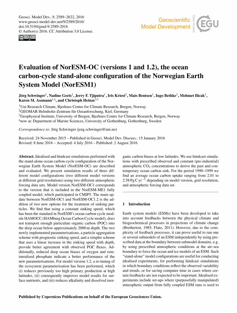
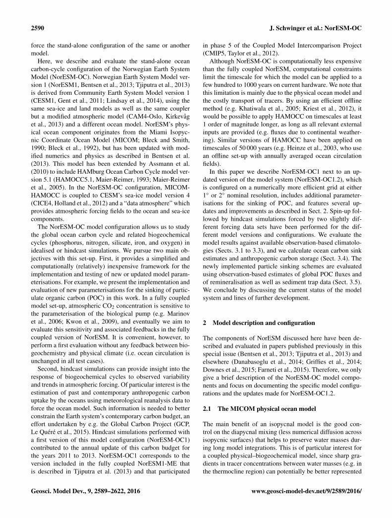
Zonal mean temperature (T ) and salinity (S) differences be-tween the model and the observation-based climatology fromWOA 2009 (Locarnini et al., 2010; Antonov et al., 2010) forthe Atlantic and Pacific basins are shown in Figs. 1 and 2. Thegeneral patterns of T and S deviations are similar across thedifferent model versions and configurations. While all threeconfigurations include salinity relaxation, this is not balancedin the case of Mv1, with the result that average salinity fallsby 0.2 units during the course of the integration. The pre-dominantly negative salinity bias for the Mv1 configurationis visible in Fig. 2. The mid-latitude and tropical regions havea too strong temperature gradient in the upper 700 m, that is,a warm bias in the upper thermocline and a cold bias below.While the magnitude and extent of the warm bias are simi-lar for the three model configurations (up to≈ 4 ◦C), the coldbias is weakest for Mv1, and strongest (up to−4 ◦C) for low-resolution configuration Lv1.2.
In the Southern Ocean south of 50◦ S, the model is gener-ally biased towards too cold and fresh conditions (about −1to−2 ◦C and up to−0.5 units on the Practical Salinity Scale)
www.geosci-model-dev.net/9/2589/2016/ Geosci. Model Dev., 9, 2589–2622, 2016
2598 J. Schwinger et al.: NorESM-OC
Dep
th [m
]
ATL, difference model−WOA
(a)
Mv1
−60 −30 0 30 60
100500
1000
3000
5000−4
−2
0
2
4
Dep
th [m
]
(c)
Mv1
.2
−60 −30 0 30 60
100500
1000
3000
5000−4
−2
0
2
4
Latitude
Dep
th [m
]
(e)
Lv1.
2
−60 −30 0 30 60
100500
1000
3000
5000−4
−2
0
2
4
PAC, difference model−WOA
(b)
−60 −30 0 30 60
100500
1000
3000
5000−4
−2
0
2
4
(d)
−60 −30 0 30 60
100500
1000
3000
5000−4
−2
0
2
4
Latitude
(f)
−60 −30 0 30 60
100500
1000
3000
5000−4
−2
0
2
4
Figure 1. Temperature difference model−WOA averaged over 1965–2007 along zonal mean sections through the Atlantic/Southern Ocean(a, c, e) and the Pacific/Southern Ocean (b, d, f) for model configurations Mv1 (a, b), Mv1.2 (c, d), and Lv1.2 (e, f). The regions covered bythe zonal mean calculations are indicated by the grey shaded area in the insets of panels (a) and (b).
Dep
th [m
]
ATL, difference model−WOA
(a)
Mv1
−60 −30 0 30 60
100500
1000
3000
5000 −0.5
0
0.5
Dep
th [m
]
(c)
Mv1
.2
−60 −30 0 30 60
100500
1000
3000
5000 −0.5
0
0.5
Latitude
Dep
th [m
]
(e)
Lv1.
2
−60 −30 0 30 60
100500
1000
3000
5000 −0.5
0
0.5
PAC, difference model−WOA
(b)
−60 −30 0 30 60
100500
1000
3000
5000 −0.5
0
0.5
(d)
−60 −30 0 30 60
100500
1000
3000
5000 −0.5
0
0.5
Latitude
(f)
−60 −30 0 30 60
100500
1000
3000
5000 −0.5
0
0.5
Figure 2. As Fig. 1 but for salinity.
Geosci. Model Dev., 9, 2589–2622, 2016 www.geosci-model-dev.net/9/2589/2016/
J. Schwinger et al.: NorESM-OC 2599
1800 1850 190012
14
16
18
20
22
24
26
28
30
32
Sv
Mv1Mv1.2Lv1.2
1948 1960 1980 2000
AMOC strength
year
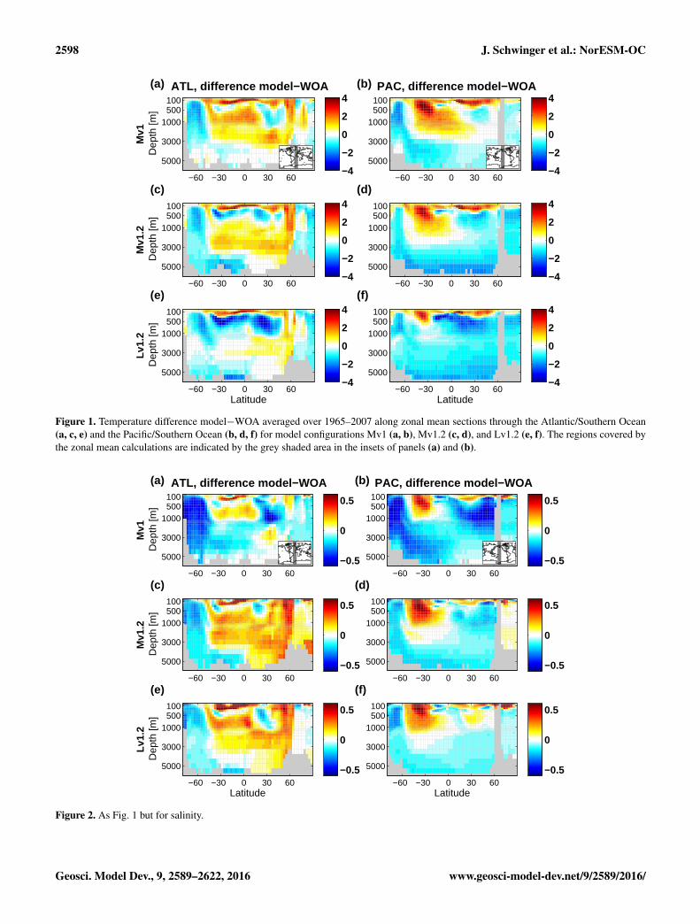
Figure 3. Atlantic Meridional Overturning Circulation (AMOC)measured as the maximum of the meridional stream-function at26.5◦ N for Mv1 (blue lines), Mv1.2 (green), and Lv1.2 (red). Theleft panel shows the AMOC for the period 1762–1947 during whichthe model is forced with the CORE normal-year forcing. In the rightpanel the years 1948–2014 are shown, and thick (thin) lines indi-cate the overturning simulated with the model forced by the NCEP-C-IAF (CORE-IAF) data set. The black diamond with error barsindicates the observational estimate provided by McCarthy et al.(2015).
below a slightly too warm surface layer. The layer of up-welled Atlantic deep water, which is warmer and more salinethan Southern Ocean surface waters, is not or only weaklypreserved in the model. At depths below 3000–4000 m thecold and fresh bias extends northwards into the Atlantic basinup to the Equator (a weak cold bias extends into the NorthAtlantic at depth). Above these bottom water masses and be-low the thermocline the Atlantic is generally too warm by1 to 2 ◦C and too saline by 0.2 to 0.5 units (again, salinityis biased low in Mv1 due to the unbalanced salinity restor-ing flux). In contrast, a warm and saline bias at intermedi-ate depths in the Pacific is mostly confined to the SouthernHemisphere, whereas the North Pacific is biased cold andfresh at all depths below 1000 m for all model configurations.We note that the cold and fresh bias in the Southern Oceanwater column is specific to the stand-alone configuration ofthe model and is not found in the fully coupled version ofNorESM (e.g. Bentsen et al., 2013, Fig. 14).
3.1.2 Atlantic Meridional Overturning Circulation
The Atlantic Meridional Overturning Circulation (AMOC)for the ocean-ice-only configuration of Mv1.2 has been com-pared to results from other models in Danabasoglu et al.(2014). The forcing protocol for this latter study was to runthe model through five cycles (1948–2007) of the CORE-IAF. The AMOC strength in our model, measured as themaximum of the annual mean meridional streamfunction at26.5◦ N, varied between 12.5 and 19 Sv and showed an in-creasing trend of roughly 1 Svcentury−1. Under the spin-upwith the CORE-NY forcing performed in the present work,
the AMOC shows a long transient increase in strength forabout 300 years before stabilising. The average overturn-ing for the 30 years before switching to interannual forcing(1918–1947) is 22.3, 24.8, and 21.5 Sv for Mv1, Mv1.2, andLv1.2, respectively (Fig. 3, left panel). Aside from the abso-lute values we find similar curves of AMOC strength underthe forcing protocol applied here (Fig. 3, right panel) com-pared to the results presented in Danabasoglu et al. (2014):first a 10- to 15-year decrease by 2 to 4 Sv followed by a rel-atively stable phase until the early 1980s, an increase by 4 to7 Sv towards a maximum in the late 1990s, and another de-crease until the end of the simulation period (2007 or 2014).The Lv1.2 configuration forced by NCEP-C-IAF is an out-lier in our small model ensemble. Compared to the othermodel simulations, the annual- and decadal-scale variabilityof AMOC strength appears to be similar but superimposedonto a negative trend of 8 Sv over the simulation period (seebelow).
In model configuration Mv1 we find only minor differ-ences in AMOC strength between the simulation forcedwith CORE-IAF and the one forced with NCEP-C-IAF. ForMv1.2 and Lv1.2, however, the CORE-IAF simulations showa weaker initial decrease and a generally larger overturn-ing than the corresponding NCEP-C-IAF simulations. Thesedifferences can be traced back to a peculiarity of the salin-ity relaxation scheme when the balancing of the relaxationflux is activated (not available in model version 1). Sincetoo much salt is taken out of the surface ocean globallyby the unbalanced scheme, negative salt fluxes are reducedby a multiplicative factor when balancing of the salinity re-laxation flux is activated. Interestingly, the global restoringsalt flux imbalance is larger when the model is forced withCORE-IAF. As a consequence of correcting this imbalance,we find a stronger reduction of the restoring salt flux out ofthe surface ocean in the simulations performed with CORE-IAF compared to those forced with NCEP-C-IAF. In the At-lantic north of 40◦ N, a positive salinity bias is thereforereinforced in the CORE-IAF simulations with model ver-sion 1.2, driving an increase in the AMOC relative to the sim-ulations forced with NCEP-C-IAF. This effect is particularlypronounced in the Lv1.2 configuration, leading to the nega-tive AMOC trend of 8 Sv described above. We note that theAMOC strength has been estimated as 17.2 Sv for the timeperiod from April 2004 to October 2012 based on observa-tions from the Rapid Climate Change programme (RAPID)array (McCarthy et al., 2015, diamond in Fig. 3). Comparedto this value, our model overestimates the AMOC strength byabout 4 to 9 Sv, except for the special case of Lv1.2 forcedwith NCEP-C-IAF discussed above, where AMOC is lowerthan the observational estimate by about 2 Sv for the periodfrom 2004 to 2012.
www.geosci-model-dev.net/9/2589/2016/ Geosci. Model Dev., 9, 2589–2622, 2016

2600 J. Schwinger et al.: NorESM-OC
J F M A M J J A S O N D0
50
100
150
200
250
N−Atlantic
m
(a)
Mv1Mv1.2Lv1.2Obs
J F M A M J J A S O N D0
50
100
150
200N−Pacific
m
(b)
J F M A M J J A S O N D0
20
40
60
80
100
120
tropics
m
(c)
A S O N D J F M A M J J0
50
100
15020 S–40 S
m
(d)
A S O N D J F M A M J J0
50
100
150
200
25040 S–60 S
m
(e)
A S O N D J F M A M J J0
50
100
150
200
250<60 S
m
(f) ooo o o
Figure 4. Mean seasonal cycle of mixed layer depth over the years 1961–2008 for the (a) North Atlantic, (b) North Pacific, (c) tropics (20◦ Sto 20◦ N), (d) southern subtropics (20 to 40◦ S), (e) latitudes between 40 and 60◦ S, and the (f) Southern Ocean south of 60◦ S. Shown areresults for model configurations Mv1 (dark blue), Mv1.2 (green), and Lv1.2 (red). The light blue line is the observation-based climatologyof de Boyer Montégut et al. (2004), which uses a density threshold criterion of 0.03 kgm−3 to define MLD.
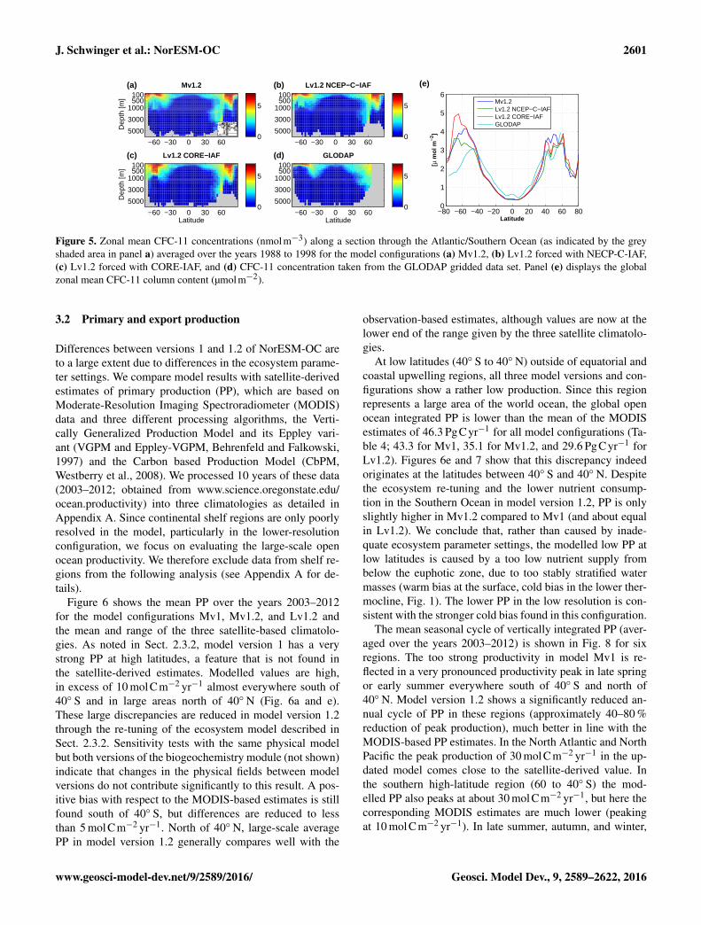
3.1.3 Mixed layer depth and CFC-11
Seasonal cycles of modelled average bulk mixed layer depth(MLD) compared to an observation-based MLD climatology(de Boyer Montégut et al., 2004) are shown for several re-gions in Fig. 4. The climatology uses a threshold criterionfor density; that is, MLD is defined by the depth where den-sity has increased by 0.03 kgm−3 relative to its near-surfacevalue. We note that the depth of the bulk mixed layer in ourmodel is calculated based on energy gain and dissipation inthe surface ocean, and that modelled and observed quanti-ties are therefore not directly comparable. A MLD clima-tology based on a density criterion is nevertheless suitablefor comparison with our model, since the criterion measuresstratification directly. We find a good agreement of mod-elled and observation-based MLD in terms of phasing andsummer minimum depth, whereas during autumn and win-ter modelled average MLDs are up to 40 to 100 m largeroutside the tropics. The largest differences are found in theSouthern Ocean south of 60◦ S (Fig. 4f) during austral win-ter. However, the observation-based climatology relies onvery few profiles during May–October in this region. Fur-ther, our calculation of model average MLD excluded ice-covered grid cells, while we have no information about howmany observed profiles taken under ice cover in the Antarc-tic entered the climatology. We therefore have little confi-dence in the model–data comparison for the southernmostSouthern Ocean during winter. In the tropics modelled aver-age MLDs are roughly 20 m larger than observed year round(i.e. about 60 vs. 40 m), with a small annual cycle that corre-sponds well to the data-based estimate. Generally, the threemodel versions and configurations show a very similar av-
erage MLD, but the low-resolution configuration Lv1.2 hasa less pronounced seasonal cycle (i.e. the winter maximumMLD is shallower and hence closer to the observation-basedestimate).
MLD averaged over large regions and time periods is notnecessarily a useful indicator of upper ocean ventilation sincespatially and temporarily localised convection events cantransport vertically large amounts of heat and matter. In fact,the modelled maximum MLD is frequently larger than 800 mover extended areas of the Southern Ocean (not shown). Thezonal mean distribution of CFC-11 in model version 1.2(Fig. 5) indicates a deeper than observed mixing compared toCFC-11 profiles from the GLODAP database. In the Atlanticsector of the Southern Ocean between 500 and 1000 m depthwe find relatively high average CFC-11 concentrations of upto 3 nmolm−3, whereas the corresponding observed CFC-11concentration is 0.44 nmolm−3. These high concentrationsare mainly caused by large fluxes occurring during Antarc-tic winter north of the ice edge. We note that forcing themodel with the NCEP-C-IAF data set tends to attenuate thedeep mixing in the Southern Ocean compared to simulationscarried out with the CORE-IAF (see Fig. 5c). In the NorthAtlantic we find frequent deep convection with maximumMLDs as deep as 1400 m in the Labrador and Irminger seasas well as in the Greenland and Norwegian seas. The compar-ison with GLODAP CFC-11 data reveals a tendency towardshigh CFC-11 concentrations located at too large depths alsoin the Labrador and Irminger seas (GLODAP does not coverthe Nordic seas). At mid latitudes we find less CFC-11 incentral and intermediate water masses, best seen as a negativebias in the modelled zonal mean integrated CFC-11 content(Fig. 5e) between 40◦ S and 40◦ N.
Geosci. Model Dev., 9, 2589–2622, 2016 www.geosci-model-dev.net/9/2589/2016/
J. Schwinger et al.: NorESM-OC 2601
Dep
th [m
]
Mv1.2
(a)
−60 −30 0 30 60
100500
1000
3000
50000
5
Lv1.2 NCEP−C−IAF
(b)
−60 −30 0 30 60
100500
1000
3000
50000
5
Latitude
Dep
th [m
]
Lv1.2 CORE−IAF
(c)
−60 −30 0 30 60
100500
1000
3000
50000
5
Latitude
GLODAP
(d)
−60 −30 0 30 60
100500
1000
3000
50000
5
−80 −60 −40 −20 0 20 40 60 800
1
2
3
4
5
6
Latitude
[µ m
ol m
−2]
(e)
Mv1.2Lv1.2 NCEP−C−IAFLv1.2 CORE−IAFGLODAP
Figure 5. Zonal mean CFC-11 concentrations (nmolm−3) along a section through the Atlantic/Southern Ocean (as indicated by the greyshaded area in panel a) averaged over the years 1988 to 1998 for the model configurations (a) Mv1.2, (b) Lv1.2 forced with NECP-C-IAF,(c) Lv1.2 forced with CORE-IAF, and (d) CFC-11 concentration taken from the GLODAP gridded data set. Panel (e) displays the globalzonal mean CFC-11 column content (µmolm−2).
3.2 Primary and export production
Differences between versions 1 and 1.2 of NorESM-OC areto a large extent due to differences in the ecosystem parame-ter settings. We compare model results with satellite-derivedestimates of primary production (PP), which are based onModerate-Resolution Imaging Spectroradiometer (MODIS)data and three different processing algorithms, the Verti-cally Generalized Production Model and its Eppley vari-ant (VGPM and Eppley-VGPM, Behrenfeld and Falkowski,1997) and the Carbon based Production Model (CbPM,Westberry et al., 2008). We processed 10 years of these data(2003–2012; obtained from www.science.oregonstate.edu/ocean.productivity) into three climatologies as detailed inAppendix A. Since continental shelf regions are only poorlyresolved in the model, particularly in the lower-resolutionconfiguration, we focus on evaluating the large-scale openocean productivity. We therefore exclude data from shelf re-gions from the following analysis (see Appendix A for de-tails).
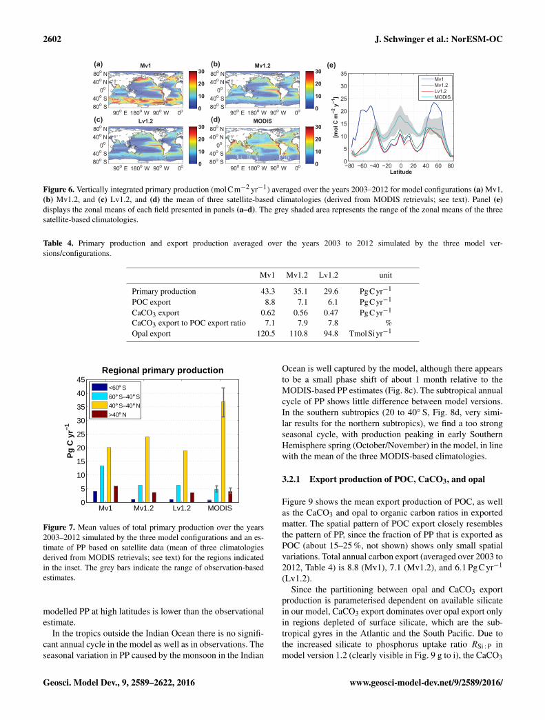
Figure 6 shows the mean PP over the years 2003–2012for the model configurations Mv1, Mv1.2, and Lv1.2 andthe mean and range of the three satellite-based climatolo-gies. As noted in Sect. 2.3.2, model version 1 has a verystrong PP at high latitudes, a feature that is not found inthe satellite-derived estimates. Modelled values are high,in excess of 10 mol Cm−2 yr−1 almost everywhere south of40◦ S and in large areas north of 40◦ N (Fig. 6a and e).These large discrepancies are reduced in model version 1.2through the re-tuning of the ecosystem model described inSect. 2.3.2. Sensitivity tests with the same physical modelbut both versions of the biogeochemistry module (not shown)indicate that changes in the physical fields between modelversions do not contribute significantly to this result. A pos-itive bias with respect to the MODIS-based estimates is stillfound south of 40◦ S, but differences are reduced to lessthan 5 molCm−2 yr−1. North of 40◦ N, large-scale averagePP in model version 1.2 generally compares well with the
observation-based estimates, although values are now at thelower end of the range given by the three satellite climatolo-gies.
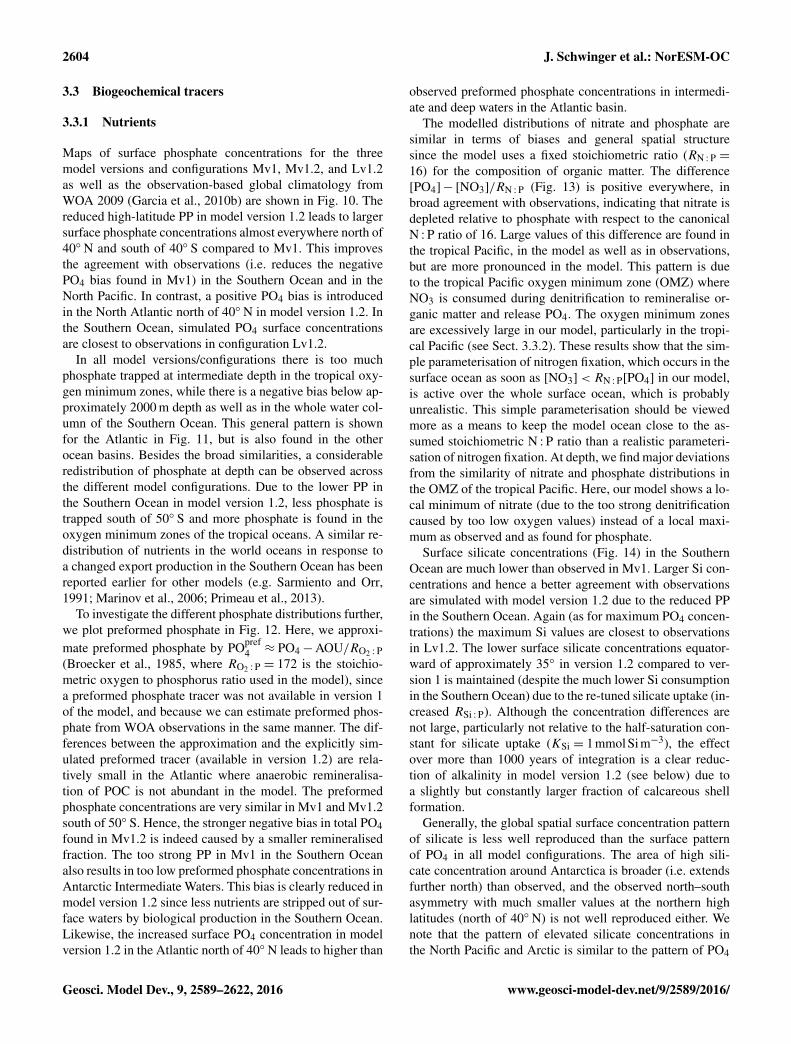
At low latitudes (40◦ S to 40◦ N) outside of equatorial andcoastal upwelling regions, all three model versions and con-figurations show a rather low production. Since this regionrepresents a large area of the world ocean, the global openocean integrated PP is lower than the mean of the MODISestimates of 46.3 PgCyr−1 for all model configurations (Ta-ble 4; 43.3 for Mv1, 35.1 for Mv1.2, and 29.6 PgCyr−1 forLv1.2). Figures 6e and 7 show that this discrepancy indeedoriginates at the latitudes between 40◦ S and 40◦ N. Despitethe ecosystem re-tuning and the lower nutrient consump-tion in the Southern Ocean in model version 1.2, PP is onlyslightly higher in Mv1.2 compared to Mv1 (and about equalin Lv1.2). We conclude that, rather than caused by inade-quate ecosystem parameter settings, the modelled low PP atlow latitudes is caused by a too low nutrient supply frombelow the euphotic zone, due to too stably stratified watermasses (warm bias at the surface, cold bias in the lower ther-mocline, Fig. 1). The lower PP in the low resolution is con-sistent with the stronger cold bias found in this configuration.
The mean seasonal cycle of vertically integrated PP (aver-aged over the years 2003–2012) is shown in Fig. 8 for sixregions. The too strong productivity in model Mv1 is re-flected in a very pronounced productivity peak in late springor early summer everywhere south of 40◦ S and north of40◦ N. Model version 1.2 shows a significantly reduced an-nual cycle of PP in these regions (approximately 40–80 %reduction of peak production), much better in line with theMODIS-based PP estimates. In the North Atlantic and NorthPacific the peak production of 30 molCm−2 yr−1 in the up-dated model comes close to the satellite-derived value. Inthe southern high-latitude region (60 to 40◦ S) the mod-elled PP also peaks at about 30 molCm−2 yr−1, but here thecorresponding MODIS estimates are much lower (peakingat 10 molCm−2 yr−1). In late summer, autumn, and winter,
www.geosci-model-dev.net/9/2589/2016/ Geosci. Model Dev., 9, 2589–2622, 2016
2602 J. Schwinger et al.: NorESM-OC
90 E 180 W 90 W 0 o o o o 80o S 40o S
0o 40o N 80 No
(a) Mv1
0
10
20
30
(b) Mv1.2
0
10
20
30
(c) Lv1.2
10
20
30
(d) MODIS
0
10
20
30
−80 −60 −40 −20 0 20 40 60 800
5
10
15
20
25
30
35
Latitude
[mol
C m
−2 y
−1]
(e)
Mv1Mv1.2Lv1.2MODIS
90 E 180 W 90 W 0 o o o o
90 E 180 W 90 W 0 o o o o 0 90 E 180 W 90 W 0 o o o o
80o S 40o S
0o 40o N 80 No
80o S 40o S
0o 40o N 80 No
80o S 40o S
0o 40o N 80 No
Figure 6. Vertically integrated primary production (molCm−2 yr−1) averaged over the years 2003–2012 for model configurations (a) Mv1,(b) Mv1.2, and (c) Lv1.2, and (d) the mean of three satellite-based climatologies (derived from MODIS retrievals; see text). Panel (e)displays the zonal means of each field presented in panels (a–d). The grey shaded area represents the range of the zonal means of the threesatellite-based climatologies.
Table 4. Primary production and export production averaged over the years 2003 to 2012 simulated by the three model ver-sions/configurations.
Mv1 Mv1.2 Lv1.2 unit
Primary production 43.3 35.1 29.6 PgCyr−1
POC export 8.8 7.1 6.1 PgCyr−1
CaCO3 export 0.62 0.56 0.47 PgCyr−1
CaCO3 export to POC export ratio 7.1 7.9 7.8 %Opal export 120.5 110.8 94.8 TmolSiyr−1
Mv1 Mv1.2 Lv1.2 MODIS0
5
10
15
20
25
30
35
40
45Regional primary production
Pg
C y
r−1
<60 S
60 S–40 S
40 S–40 N
>40 N
o
o o
o o
o
Figure 7. Mean values of total primary production over the years2003–2012 simulated by the three model configurations and an es-timate of PP based on satellite data (mean of three climatologiesderived from MODIS retrievals; see text) for the regions indicatedin the inset. The grey bars indicate the range of observation-basedestimates.
modelled PP at high latitudes is lower than the observationalestimate.
In the tropics outside the Indian Ocean there is no signifi-cant annual cycle in the model as well as in observations. Theseasonal variation in PP caused by the monsoon in the Indian
Ocean is well captured by the model, although there appearsto be a small phase shift of about 1 month relative to theMODIS-based PP estimates (Fig. 8c). The subtropical annualcycle of PP shows little difference between model versions.In the southern subtropics (20 to 40◦ S, Fig. 8d, very simi-lar results for the northern subtropics), we find a too strongseasonal cycle, with production peaking in early SouthernHemisphere spring (October/November) in the model, in linewith the mean of the three MODIS-based climatologies.
3.2.1 Export production of POC, CaCO3, and opal
Figure 9 shows the mean export production of POC, as wellas the CaCO3 and opal to organic carbon ratios in exportedmatter. The spatial pattern of POC export closely resemblesthe pattern of PP, since the fraction of PP that is exported asPOC (about 15–25 %, not shown) shows only small spatialvariations. Total annual carbon export (averaged over 2003 to2012, Table 4) is 8.8 (Mv1), 7.1 (Mv1.2), and 6.1 PgCyr−1
(Lv1.2).Since the partitioning between opal and CaCO3 export
production is parameterised dependent on available silicatein our model, CaCO3 export dominates over opal export onlyin regions depleted of surface silicate, which are the sub-tropical gyres in the Atlantic and the South Pacific. Due tothe increased silicate to phosphorus uptake ratio RSi :P inmodel version 1.2 (clearly visible in Fig. 9 g to i), the CaCO3
Geosci. Model Dev., 9, 2589–2622, 2016 www.geosci-model-dev.net/9/2589/2016/

J. Schwinger et al.: NorESM-OC 2603
J F M A M J J A S O N D0
20
40
60
N−Atlantic
mol
C m
−2 y
r−2
Mv1Mv1.2Lv1.2MODIS
(a)
J F M A M J J A S O N D0
20
40
60
N−Pacific
mol
C m
−2 y
r−2
(b)
J F M A M J J A S O N D0
10
20
30
Tropical Indian Ocean
mol
C m
−2 y
r−2
(c)
A S O N D J F M A M J J0
5
10
15
2020 S–40 S
mol
C m
−2 y
r−2
(d)
A S O N D J F M A M J J0
20
40
60
8040 S–60 S
mol
C m
−2 y
r−2
(e)
A S O N D J F M A M J J0
20
40
60
80<60 S
mol
C m
−2 y
r−2
(f)ooooo
Figure 8. Mean seasonal cycle of vertically integrated primary production over the years 2003–2012 for the (a) North Atlantic, (b) NorthPacific, (c) tropical Indian Ocean (Indian Ocean between 20◦ S and 20◦ N), (d) southern subtropics (40 to 20◦ S), (e) latitudes between 60and 40◦ S, and the (f) Southern Ocean south of 60◦ S. Shown are the results for model configurations Mv1 (dark blue), Mv1.2 (green), andLv1.2 (red) and the mean and range of the satellite-derived seasonal cycle (light blue and grey shaded areas).
Figure 9. Export production of POC averaged over the years 2003–2012 for the model configurations (a) Mv1, (b) Mv1.2, and (c) Lv1.2;corresponding CaCO3 to organic carbon ratio in exported matter for (d) Mv1, (e) Mv1.2, and (f) Lv1.2; corresponding opal to organic carbonratio in exported matter for (g) Mv1, (h) Mv1.2, and (i) Lv1.2.
production is maintained or even slightly expanded into thewestern North Pacific despite the much lower PP (and sur-face silicate consumption) at high latitudes in this model ver-sion. We note that the simple parameterisation of opal andCaCO3 export production is qualitatively supported by opalto particulate inorganic carbon (PIC) ratios derived from sed-iment traps. For example, Honjo et al. (2008, see their Fig. 7)show that high opal/PIC ratios are constrained to ocean re-
gions with high surface silica concentrations, a pattern that isqualitatively reproduced by our model.
Total modelled opal export (between 95 and120.5 TmolSiyr−1, Table 4) is within the uncertaintyrange of the estimate of 105± 17 TmolSiyr−1 given byTréguer and De La Rocha (2013). The ratio of CaCO3 exportto organic carbon export of 7.1 to 7.9 % is within the rangeestimated by Sarmiento et al. (2002, 6± 3 %).
www.geosci-model-dev.net/9/2589/2016/ Geosci. Model Dev., 9, 2589–2622, 2016
2604 J. Schwinger et al.: NorESM-OC
3.3 Biogeochemical tracers
3.3.1 Nutrients
Maps of surface phosphate concentrations for the threemodel versions and configurations Mv1, Mv1.2, and Lv1.2as well as the observation-based global climatology fromWOA 2009 (Garcia et al., 2010b) are shown in Fig. 10. Thereduced high-latitude PP in model version 1.2 leads to largersurface phosphate concentrations almost everywhere north of40◦ N and south of 40◦ S compared to Mv1. This improvesthe agreement with observations (i.e. reduces the negativePO4 bias found in Mv1) in the Southern Ocean and in theNorth Pacific. In contrast, a positive PO4 bias is introducedin the North Atlantic north of 40◦ N in model version 1.2. Inthe Southern Ocean, simulated PO4 surface concentrationsare closest to observations in configuration Lv1.2.
In all model versions/configurations there is too muchphosphate trapped at intermediate depth in the tropical oxy-gen minimum zones, while there is a negative bias below ap-proximately 2000 m depth as well as in the whole water col-umn of the Southern Ocean. This general pattern is shownfor the Atlantic in Fig. 11, but is also found in the otherocean basins. Besides the broad similarities, a considerableredistribution of phosphate at depth can be observed acrossthe different model configurations. Due to the lower PP inthe Southern Ocean in model version 1.2, less phosphate istrapped south of 50◦ S and more phosphate is found in theoxygen minimum zones of the tropical oceans. A similar re-distribution of nutrients in the world oceans in response toa changed export production in the Southern Ocean has beenreported earlier for other models (e.g. Sarmiento and Orr,1991; Marinov et al., 2006; Primeau et al., 2013).
To investigate the different phosphate distributions further,we plot preformed phosphate in Fig. 12. Here, we approxi-mate preformed phosphate by POpref
4 ≈ PO4−AOU/RO2 :P(Broecker et al., 1985, where RO2 :P = 172 is the stoichio-metric oxygen to phosphorus ratio used in the model), sincea preformed phosphate tracer was not available in version 1of the model, and because we can estimate preformed phos-phate from WOA observations in the same manner. The dif-ferences between the approximation and the explicitly sim-ulated preformed tracer (available in version 1.2) are rela-tively small in the Atlantic where anaerobic remineralisa-tion of POC is not abundant in the model. The preformedphosphate concentrations are very similar in Mv1 and Mv1.2south of 50◦ S. Hence, the stronger negative bias in total PO4found in Mv1.2 is indeed caused by a smaller remineralisedfraction. The too strong PP in Mv1 in the Southern Oceanalso results in too low preformed phosphate concentrations inAntarctic Intermediate Waters. This bias is clearly reduced inmodel version 1.2 since less nutrients are stripped out of sur-face waters by biological production in the Southern Ocean.Likewise, the increased surface PO4 concentration in modelversion 1.2 in the Atlantic north of 40◦ N leads to higher than
observed preformed phosphate concentrations in intermedi-ate and deep waters in the Atlantic basin.
The modelled distributions of nitrate and phosphate aresimilar in terms of biases and general spatial structuresince the model uses a fixed stoichiometric ratio (RN : P =
16) for the composition of organic matter. The difference[PO4] − [NO3]/RN : P (Fig. 13) is positive everywhere, inbroad agreement with observations, indicating that nitrate isdepleted relative to phosphate with respect to the canonicalN : P ratio of 16. Large values of this difference are found inthe tropical Pacific, in the model as well as in observations,but are more pronounced in the model. This pattern is dueto the tropical Pacific oxygen minimum zone (OMZ) whereNO3 is consumed during denitrification to remineralise or-ganic matter and release PO4. The oxygen minimum zonesare excessively large in our model, particularly in the tropi-cal Pacific (see Sect. 3.3.2). These results show that the sim-ple parameterisation of nitrogen fixation, which occurs in thesurface ocean as soon as [NO3]<RN : P[PO4] in our model,is active over the whole surface ocean, which is probablyunrealistic. This simple parameterisation should be viewedmore as a means to keep the model ocean close to the as-sumed stoichiometric N : P ratio than a realistic parameteri-sation of nitrogen fixation. At depth, we find major deviationsfrom the similarity of nitrate and phosphate distributions inthe OMZ of the tropical Pacific. Here, our model shows a lo-cal minimum of nitrate (due to the too strong denitrificationcaused by too low oxygen values) instead of a local maxi-mum as observed and as found for phosphate.
Surface silicate concentrations (Fig. 14) in the SouthernOcean are much lower than observed in Mv1. Larger Si con-centrations and hence a better agreement with observationsare simulated with model version 1.2 due to the reduced PPin the Southern Ocean. Again (as for maximum PO4 concen-trations) the maximum Si values are closest to observationsin Lv1.2. The lower surface silicate concentrations equator-ward of approximately 35◦ in version 1.2 compared to ver-sion 1 is maintained (despite the much lower Si consumptionin the Southern Ocean) due to the re-tuned silicate uptake (in-creased RSi : P). Although the concentration differences arenot large, particularly not relative to the half-saturation con-stant for silicate uptake (KSi = 1mmolSim−3), the effectover more than 1000 years of integration is a clear reduc-tion of alkalinity in model version 1.2 (see below) due toa slightly but constantly larger fraction of calcareous shellformation.
Generally, the global spatial surface concentration patternof silicate is less well reproduced than the surface patternof PO4 in all model configurations. The area of high sili-cate concentration around Antarctica is broader (i.e. extendsfurther north) than observed, and the observed north–southasymmetry with much smaller values at the northern highlatitudes (north of 40◦ N) is not well reproduced either. Wenote that the pattern of elevated silicate concentrations inthe North Pacific and Arctic is similar to the pattern of PO4
Geosci. Model Dev., 9, 2589–2622, 2016 www.geosci-model-dev.net/9/2589/2016/
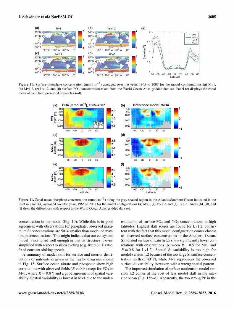
J. Schwinger et al.: NorESM-OC 2605
90 E 180 W 90 W 0 o o o o 80o S 40o S
0o 40o N 80o N
(a) Mv1
0
1
2
(b) Mv1.2
0
1
2
(c) Lv1.2
0
1
2
(d) WOA
0
1
2
−80 −60 −40 −20 0 20 40 60 800
0.5
1
1.5
2
Latitude
[mm
ol m
−3]
(e)
Mv1Mv1.2Lv1.2WOA
90 E 180 W 90 W 0 o o o o 80o S 40o S
0o 40o N 80o N
90 E 180 W 90 W 0 o o o o 80o S 40o S
0o 40o N 80o N
90 E 180 W 90 W 0 o o o o 80o S 40o S
0o 40o N 80o N
Figure 10. Surface phosphate concentration (mmolm−3) averaged over the years 1965 to 2007 for the model configurations (a) Mv1,(b) Mv1.2, (c) Lv1.2, and (d) surface PO4 concentration taken from the World Ocean Atlas gridded data set. Panel (e) displays the zonalmean of each field presented in panels (a–d).
Dep
th [m
]
PO4 [mmol m ], 1965–2007−3
(a)
Mv1
−60 −30 0 30 60
100500
1000
3000
5000 0.511.522.5
Dep
th [m
]
(c)
Mv1
.2
−60 −30 0 30 60
100500
1000
3000
5000 0.511.522.5
Latitude
Dep
th [m
]
(e)
Lv1.
2
−60 −30 0 30 60
100500
1000
3000
5000 0.511.522.5
Difference model−WOA
(b)
−60 −30 0 30 60
100500
1000
3000
5000−1
0
1
(d)
−60 −30 0 30 60
100500
1000
3000
5000−1
0
1
Latitude
(f)
−60 −30 0 30 60
100500
1000
3000
5000−1
0
1
Figure 11. Zonal mean phosphate concentration (mmolm−3) along the grey shaded region in the Atlantic/Southern Ocean indicated in theinset in panel (a) averaged over the years 1965 to 2007 for the model configurations (a) Mv1, (c) Mv1.2, and (e) Lv1.2. Panels (b), (d), and(f) show the differences with respect to the World Ocean Atlas gridded data set.
concentration in the model (Fig. 10). While this is in goodagreement with observations for phosphate, observed maxi-mum Si concentrations are 50 % smaller than modelled max-imum concentrations. This might indicate that our ecosystemmodel is not tuned well enough or that its structure is over-simplified with respect to silica cycling (e.g. fixed Si : P ratio,fixed constant sinking speed).
A summary of model skill for surface and interior distri-butions of nutrients is given in the Taylor diagrams shownin Fig. 15. Surface ocean nitrate and phosphate show highcorrelations with observed fields (R > 0.9 except for PO4 inMv1, where R = 0.87) and a good agreement of spatial vari-ability. Spatial variability is lowest in Mv1 due to the under-
estimation of surface PO4 and NO3 concentrations at highlatitudes. Highest skill scores are found for Lv1.2, consis-tent with the fact that this model configuration comes closestto observed surface concentrations in the Southern Ocean.Simulated surface silicate fields show significantly lower cor-relations with observations (between R = 0.5 for Mv1 andR = 0.8 for Lv1.2). Spatial Si variability is too high formodel version 1.2 because of the too large Si surface concen-tration north of 40◦ N, while Mv1 reproduces the observedsurface Si variability, however, with a wrong spatial pattern.
The improved simulation of surface nutrients in model ver-sion 1.2 comes at the cost of less model skill in the inte-rior ocean (Fig. 15b–d). Apparently, the too strong PP in the
www.geosci-model-dev.net/9/2589/2016/ Geosci. Model Dev., 9, 2589–2622, 2016
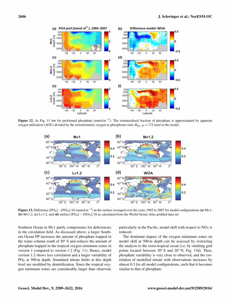
2606 J. Schwinger et al.: NorESM-OC
Dep
th [m
]
PO4 pref [mmol m ], 1965–2007−3
(a)
Mv1
−60 −30 0 30 60
100500
1000
3000
50000
1
2
Dep
th [m
]
(c)
Mv1
.2
−60 −30 0 30 60
100500
1000
3000
50000
1
2
Latitude
Dep
th [m
]
(e)
Lv1.
2
−60 −30 0 30 60
100500
1000
3000
50000
1
2
Difference model−WOA
(b)
−60 −30 0 30 60
100500
1000
3000
5000−0.5
0
0.5
(d)
−60 −30 0 30 60
100500
1000
3000
5000−0.5
0
0.5
Latitude
(f)
−60 −30 0 30 60
100500
1000
3000
5000−0.5
0
0.5
Figure 12. As Fig. 11 but for preformed phosphate (mmolm−3). The remineralised fraction of phosphate is approximated by apparentoxygen utilisation (AOU) divided by the stoichiometric oxygen to phosphorus ratio RO2 :P = 172 used in the model.
90o E 180o W 90o W 0o 80o S
40o S
0o
40o N
80o N
(a) Mv1
0.2
0.4
80o S
40o S
0o
40o N
80o N
(b) Mv1.2
0.2
0.4
80o S
40o S
0o
40o N
80o N
(c) Lv1.2
0.2
0.4
80o S
40o S
0o
40o N
80o N
(d) WOA
0.2
0.4
90o E 180o W 90o W 0o
90o E 180o W 90o W 0o 90o E 180o W 90o W 0o
Figure 13. Difference [PO4]−[NO3]/16 (mmolm−3) at the surface averaged over the years 1965 to 2007 for model configurations (a) Mv1,(b) Mv1.2, (c) Lv1.2, and (d) surface [PO4] − [NO3]/16 as calculated from the World Ocean Atlas gridded data set.
Southern Ocean in Mv1 partly compensates for deficienciesin the circulation field. As discussed above, a larger South-ern Ocean PP increases the amount of phosphate trapped inthe water column south of 50◦ S and reduces the amount ofphosphate trapped in the tropical oxygen minimum zones inversion 1 compared to version 1.2 (Fig. 11). Hence, modelversion 1.2 shows less correlation and a larger variability ofPO4 at 500 m depth. Simulated nitrate fields at this depthlevel are modified by denitrification. Since the tropical oxy-gen minimum zones are considerably larger than observed,
particularly in the Pacific, model skill with respect to NO3 isreduced.
The dominant impact of the oxygen minimum zones onmodel skill at 500 m depth can be assessed by restrictingthe analysis to the extra-tropical ocean (i.e. by omitting gridpoints located between 20◦ S and 20◦ N, Fig. 15d). Then,phosphate variability is very close to observed, and the cor-relation of modelled nitrate with observations increases byalmost 0.3 for all model configurations, such that it becomessimilar to that of phosphate.
Geosci. Model Dev., 9, 2589–2622, 2016 www.geosci-model-dev.net/9/2589/2016/
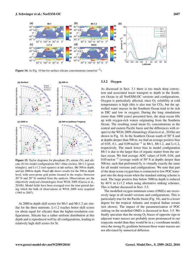
J. Schwinger et al.: NorESM-OC 2607
90 E 180 W 90 W 0
(a) (b)
(c) (d)
(e)
90 E 180 W 90 W 0
90 E 180 W 90 W 0 90 E 180 W 90 W 0
Figure 14. As Fig. 10 but for surface silicate concentrations (mmolm−3).
Nor
mal
ized
sta
ndar
d de
viat
ion
0
1
0.5
1
1
0.99
0.95
0.9
0.8
0.70.6
0.50.4
0.30.20.10 Cor relat ion oef f i c ient
RM
SD
obsN
P
S
N
P
S
N
P
S
(a) Surface
Mv1Mv1.2Lv1.2
Nor
mal
ized
sta
ndar
d de
viat
ion
0
1
0.5
1
1
0.99
0.95
0.9
0.8
0.70.6
0.50.4
0.30.20.10 Cor relat ion oef f i c ient
RM
SD
obs
N
P
SN PSN P
S
(b) 500 m
Nor
mal
ized
sta
ndar
d de
viat
ion
0
1
0
2
0.5
1
1
0.99
0.95
0.9
0.8
0.70.6
0.50.4
0.30.20.10 Cor relat ion oef f i c ient
RM
SD
obs
NP
S
N
P
S
N
P
S
(c) 2000 m
Nor
mal
ized
sta
ndar
d de
viat
ion
0
1
0.5
1
1
0.99
0.95
0.9
0.8
0.70.6
0.50.4
0.30.20.10 Cor relat ion oef f i c ient
RM
SD
obs
N
PS
N
P
S
N
P
S
(d) 500 m (without Tropics)
c c
c c
Figure 15. Taylor diagrams for phosphate (P), nitrate (N), and sili-cate (S) for model configurations Mv1 (blue circles), Mv1.2 (greentriangles), and Lv1.2 (red squares) at (a) surface, (b) 500 m depth,and (c) 2000 m depth. Panel (d) shows results for the 500 m depthlevel, with error-prone grid points located in the tropics (between20◦ N and 20◦ S) omitted from the analysis. Observations are theobjectively analysed climatologies from WOA 2009 (Garcia et al.,2010b). Model fields have been averaged over the time period dur-ing which the bulk of observations in WOA 2009 were acquired(1965 to 2007).
At 2000 m depth skill scores for Mv1 and Mv1.2 are sim-ilar for the three nutrients. Lv1.2 reaches better skill scores(or about equal for silicate) than the higher-resolution con-figurations. Silicate has a rather uniform distribution at thisdepth and is reproduced well by all configurations, leading torelatively high skill scores for Si.
3.3.2 Oxygen
As discussed in Sect. 3.1 there is too much deep convec-tion and associated tracer transport to depth in the South-ern Ocean in all NorESM-OC versions and configurations.Oxygen is particularly affected, since O2 solubility at coldtemperatures is high (this is also true for CO2, but the up-welled water masses in the Southern Ocean tend to be richin DIC and low in oxygen). During the long simulations(more than 1000 years) presented here, the deep ocean fillsup with oxygen-rich waters originating from the SouthernOcean. The resulting zonal mean O2 concentrations in thecentral and eastern Pacific basin and the differences with re-spect to the WOA 2009 climatology (Garcia et al., 2010a) areshown in Fig. 16. In the Southern Ocean south of 50◦ S andat depths deeper than 500 m, we find an average positive biasof 0.05, 0.1, and 0.09 molm−3 in Mv1, Mv1.2, and Lv1.2,respectively. The much lower bias in model configurationMv1 is due to the larger flux of organic matter from the sur-face ocean. We find average AOU values of 0.09, 0.04, and0.05 molm−3 (average south of 50◦ S at depths deeper than500 m), such that preformed O2 is virtually exactly the samefor all model versions and configurations. We note that partof the deep ocean oxygen bias is connected to low POC trans-port into the deep ocean when the standard sinking scheme isused. The large positive bias below 3000 m depth is reducedby 40 % in Lv1.2 when using alternative sinking schemes.This is further discussed in Sect. 3.5.
The modelled oxygen minimum zones (OMZs) are exces-sively large in all model versions and configurations. This isparticularly true for the Pacific basin (Fig. 16), and to a lesserdegree for the tropical Atlantic and tropical Indian oceans(not shown). The impact of the parameterisation of POCsinking on the modelled OMZs is discussed in Sect. 3.5. Wefinally speculate that the strong O2 biases of opposite sign inadjacent water masses are probably more pronounced in ourisopycnic model than they would be in a z-coordinate model,since the strong O2 gradients between these water masses arenot alleviated by numerical diffusion.
www.geosci-model-dev.net/9/2589/2016/ Geosci. Model Dev., 9, 2589–2622, 2016
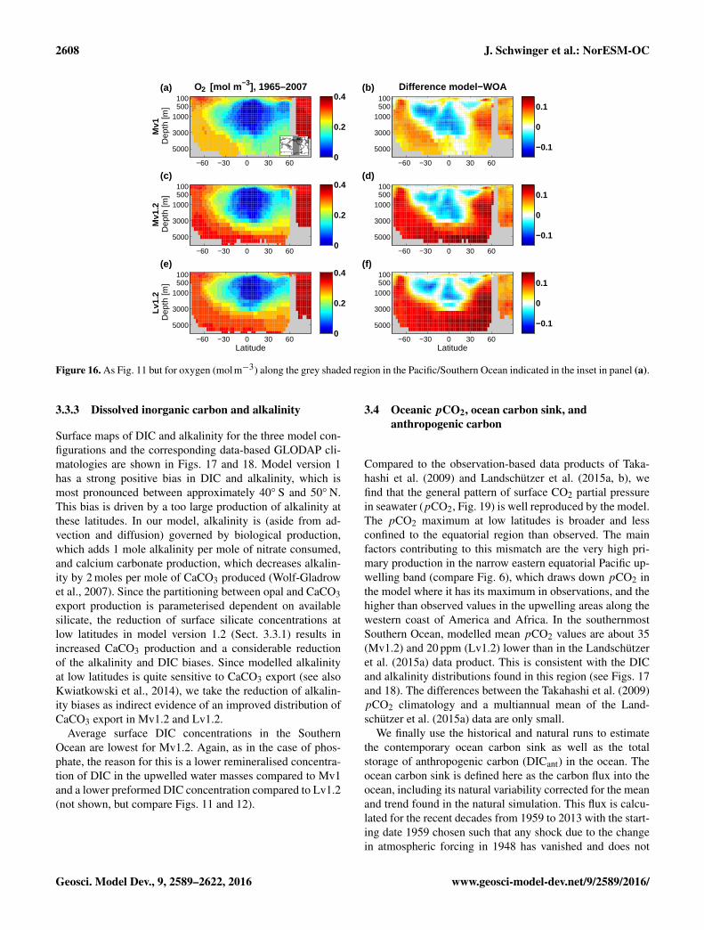
2608 J. Schwinger et al.: NorESM-OC
Dep
th [m
]
O [mol m ], 1965–2007−3
(a)
Mv1
−60 −30 0 30 60
100500
1000
3000
50000
0.2
0.4
Dep
th [m
]
(c)
Mv1
.2
−60 −30 0 30 60
100500
1000
3000
50000
0.2
0.4
Latitude
Dep
th [m
]
(e)
Lv1.
2
−60 −30 0 30 60
100500
1000
3000
50000
0.2
0.4
Difference model−WOA
(b)
−60 −30 0 30 60
100500
1000
3000
5000 −0.1
0
0.1
(d)
−60 −30 0 30 60
100500
1000
3000
5000 −0.1
0
0.1
Latitude
(f)
−60 −30 0 30 60
100500
1000
3000
5000 −0.1
0
0.1
2
Figure 16. As Fig. 11 but for oxygen (molm−3) along the grey shaded region in the Pacific/Southern Ocean indicated in the inset in panel (a).
3.3.3 Dissolved inorganic carbon and alkalinity
Surface maps of DIC and alkalinity for the three model con-figurations and the corresponding data-based GLODAP cli-matologies are shown in Figs. 17 and 18. Model version 1has a strong positive bias in DIC and alkalinity, which ismost pronounced between approximately 40◦ S and 50◦ N.This bias is driven by a too large production of alkalinity atthese latitudes. In our model, alkalinity is (aside from ad-vection and diffusion) governed by biological production,which adds 1 mole alkalinity per mole of nitrate consumed,and calcium carbonate production, which decreases alkalin-ity by 2 moles per mole of CaCO3 produced (Wolf-Gladrowet al., 2007). Since the partitioning between opal and CaCO3export production is parameterised dependent on availablesilicate, the reduction of surface silicate concentrations atlow latitudes in model version 1.2 (Sect. 3.3.1) results inincreased CaCO3 production and a considerable reductionof the alkalinity and DIC biases. Since modelled alkalinityat low latitudes is quite sensitive to CaCO3 export (see alsoKwiatkowski et al., 2014), we take the reduction of alkalin-ity biases as indirect evidence of an improved distribution ofCaCO3 export in Mv1.2 and Lv1.2.
Average surface DIC concentrations in the SouthernOcean are lowest for Mv1.2. Again, as in the case of phos-phate, the reason for this is a lower remineralised concentra-tion of DIC in the upwelled water masses compared to Mv1and a lower preformed DIC concentration compared to Lv1.2(not shown, but compare Figs. 11 and 12).
3.4 Oceanic pCO2, ocean carbon sink, andanthropogenic carbon
Compared to the observation-based data products of Taka-hashi et al. (2009) and Landschützer et al. (2015a, b), wefind that the general pattern of surface CO2 partial pressurein seawater (pCO2, Fig. 19) is well reproduced by the model.The pCO2 maximum at low latitudes is broader and lessconfined to the equatorial region than observed. The mainfactors contributing to this mismatch are the very high pri-mary production in the narrow eastern equatorial Pacific up-welling band (compare Fig. 6), which draws down pCO2 inthe model where it has its maximum in observations, and thehigher than observed values in the upwelling areas along thewestern coast of America and Africa. In the southernmostSouthern Ocean, modelled mean pCO2 values are about 35(Mv1.2) and 20 ppm (Lv1.2) lower than in the Landschützeret al. (2015a) data product. This is consistent with the DICand alkalinity distributions found in this region (see Figs. 17and 18). The differences between the Takahashi et al. (2009)pCO2 climatology and a multiannual mean of the Land-schützer et al. (2015a) data are only small.
We finally use the historical and natural runs to estimatethe contemporary ocean carbon sink as well as the totalstorage of anthropogenic carbon (DICant) in the ocean. Theocean carbon sink is defined here as the carbon flux into theocean, including its natural variability corrected for the meanand trend found in the natural simulation. This flux is calcu-lated for the recent decades from 1959 to 2013 with the start-ing date 1959 chosen such that any shock due to the changein atmospheric forcing in 1948 has vanished and does not
Geosci. Model Dev., 9, 2589–2622, 2016 www.geosci-model-dev.net/9/2589/2016/

J. Schwinger et al.: NorESM-OC 2609
(a) (b)
(c) (d)
(e)
Figure 17. Surface concentration of dissolved inorganic carbon (molm−3) averaged over the years 1988 to 1998 for the model configurations(a) Mv1, (b) Mv1.2, and (c) Lv1.2, and (d) corresponding surface DIC from the observation-based GLODAP climatology. Panel (e) displaysthe zonal mean of each field presented in panels (a–d).
90 E 180 W 90 W 0 o o o o 80o S 40o S
0o 40o N 80o N
(a) Mv1
2.2
2.4
2.6
80o S 40o S
0o 40o N 80o N
(b) Mv1.2
2.2
2.4
2.6
80o S 40o S
0o 40o N 80o N
(c) Lv1.2
2.2
2.4
2.6
80o S 40o S
0o 40o N 80o N
(d) GLODAP
2.2
2.4
2.6
−80 −60 −40 −20 0 20 40 60 802.2
2.3
2.4
2.5
2.6
Latitude
[eq
m−3
]
(e)
Mv1Mv1.2Lv1.2GLODAP
90 E 180 W 90 W 0 o o o o
90 E 180 W 90 W 0 o o o o 90 E 180 W 90 W 0 o o o o
Figure 18. As Fig. 17 but for surface total alkalinity (eqm−3).
influence the calculation of trends. Results for the differentmodel versions and configurations forced with NCEP-C-IAFand CORE-IAF are shown in Fig. 20.
The simulated ocean carbon sink is largest for model ver-sion 1, with a mean carbon sink of 2.58 and 2.50 PgCyr−1
during 1990 to 1999 when forced with the NCEP-C-IAF andCORE-IAF, respectively (Table 5). The accumulated uptakeover 1959 to 2007 for this model version and the two forc-ing data sets differs in the same proportion (102 vs. 99 PgC).Model version 1.2 shows a lower ocean carbon sink with amean value of 2.33 PgCyr−1 over the 1990 to 1999 periodfor the medium-resolution configuration (2.46 when forcedwith CORE-IAF). The corresponding numbers for the low-resolution simulation forced with the NCEP-C and CORE-IAF are 2.01 and 2.24 PgCyr−1, respectively. We comparethese model results to the three independent data-based es-timates (grey symbols with error bars in Fig. 20) of McNeilet al. (2003), 2.0± 0.4 PgCyr−1 over 1990–1999, Manningand Keeling (2006), 1.9±0.6 PgCyr−1 over 1990–2000, andMikaloff Fletcher et al. (2006), 2.2±0.25 PgCyr−1 for 1995,which are the basis for the ocean sink value given in the Inter-governmental Panel on Climate Change Fourth AssessmentReport (Denman et al., 2007), and which are also used as the
data-based ocean sink estimate in Le Quéré et al. (2015). Thesimulated ocean sink appears to be too large in Mv1, whilefor version 1.2 the sink estimates are within the error barsof the data-based estimates. The closest match is found forthe low-resolution configuration forced with NCEP-C-IAF,which has the lowest carbon uptake. The rather too high CO2uptake is confirmed when comparing the model results tothe CO2 flux estimates of Landschützer et al. (2015a). Thereis a relatively good agreement with the CO2 sink simulatedwith Lv1.2 up to 1990 and towards the end of the time se-ries (year 2011). From the early 1990s until 2001, the Land-schützer et al. (2015a) data show a marked decline followedby a steep increase in carbon uptake, which they attributeto a saturation followed by a reinvigoration of the SouthernOcean carbon sink. Although our model also shows a stag-nation of the ocean carbon sink during the 1990s, there isno pronounced minimum and hence a rather large deviationfrom the Landschützer et al. (2015a) data around the year2000.
Also compared to results of similar ocean biogeochemicalmodels forced with reanalysis data (Le Quéré et al., 2015, seeFig. 21 for names and references of individual models), thecarbon uptake of NorESM-OC appears to be large. Figure 21
www.geosci-model-dev.net/9/2589/2016/ Geosci. Model Dev., 9, 2589–2622, 2016

2610 J. Schwinger et al.: NorESM-OC
90 E 180 W 90 W 0 o o o o 80o S 40o S
0o 40o N 80o N
(a) Mv1
350
400
450
80o S 40o S
0o 40o N 80o N
(b) Mv1.2
350
400
450
80o S 40o S
0o 40o N 80o N
(c) Lv1.2
350
400
450
80o S 40o S
0o 40o N 80o N
(d) LA15
350
400
450
−80 −60 −40 −20 0 20 40 60 80300
320
340
360
380
400
Latitude
[µ a
tm]
(e)
Mv1Mv1.2Lv1.2LA15TA09
90 E 180 W 90 W 0 o o o o
90 E 180 W 90 W 0 o o o o 90 E 180 W 90 W 0 o o o o
Figure 19. Surface partial pressure of CO2 (µatm) averaged over the years 1995 to 2005 for model configurations (a) Mv1, (b) Mv1.2,(c) Lv1.2, and (d) the observation-based surface pCO2 data set of Landschützer et al. (2015a). Panel (e) displays the zonal mean of eachfield presented in panels (a–d) and additionally the zonal mean of the data product by Takahashi et al. (2009). The black line indicates themean atmospheric pCO2 over the averaging period.
Table 5. Estimates of the ocean carbon sink, accumulated carbon uptake, and anthropogenic DIC simulated by the three model ver-sions/configurations. Numbers in parentheses are results from the model forced with the CORE-IAF forcing. The second to last columngives corresponding observation-based estimates.
Year Mv1 Mv1.2 Lv1.2 Obs Unit
C sink 1990–1999 2.58 (2.50) 2.33 (2.46) 2.01 (2.24) 2.0± 0.44a PgCyr−1
Acc. C uptake 1959–2007 102 (99) 93.0 (95.6) 83.7 (88.4) — PgCDICant 1994 141 (139) 133 (134) 122 (123) 118± 19b PgCDICant 2010 186 175 159 155± 31c PgC
a This is the weighted (by uncertainty) mean of the estimates of McNeil et al. (2003), Manning and Keeling (2006), and Mikaloff Fletcher et al.(2006). The given uncertainty is the root mean square of the individual error estimates.b Sabine et al. (2004)c Khatiwala et al. (2013)
shows that, after 1980, the carbon sink in Mv1 and Mv1.2 isabove the range of other models, while Lv1.2 is at the upperend of the range.
The anthropogenic dissolved inorganic carbon (DICant)stored in the ocean is displayed in Fig. 22 for the year 1994,and corresponding total numbers are given in Table 5. Con-sistent with the larger than observed carbon sink fluxes, ourmodel also shows higher anthropogenic carbon storage com-pared to the Sabine et al. (2004) estimate of DICant avail-able from the GLODAP database. In the North Atlantic mod-elled anthropogenic carbon is larger than observed, which isconsistent with the too strong simulated AMOC. Model ver-sion 1.2 has a stronger AMOC when simulations are forcedwith the CORE-IAF (see Sect. 3.1.2), and we find a largeraccumulation of DICant in the North Atlantic for this forcing(not shown), consistent with the larger (accumulated) uptakeflux (Fig. 20). In the Southern Ocean the too high concen-tration of DICant is consistent with the too strong ventila-tion diagnosed from the CFC-11 tracer (Sect. 3.1.3). Largerthan observed DICant concentrations are also found north of40◦ S, where DIC is subducted in Antarctic Intermediate Wa-ters. Compared to a recent synthesis of anthropogenic carbonstorage estimates (Khatiwala et al., 2013, 155± 31 PgC for
the year 2010), modelled DICant storage of 186 (Mv1), 175(Mv1.2), and 159 (Lv1.2) PgC is higher but still within theuncertainty range of the synthesis estimate.
3.5 Particle export and sedimentation
To evaluate the three different sinking schemes avail-able in NorESM-OC1.2, we conducted a spin-up run over1000 years for each scheme using the low-resolution configu-ration of the model. In addition we performed one sensitivityexperiment employing the standard option, but with the con-stant POC sinking speed increased from 5 to 14 md−1. Thesetwo runs are referred to as STD-slow and STD-fast, respec-tively, while the model runs employing the prognostic parti-cle aggregation scheme (Kriest, 2002) and the linear increasein sinking speed are abbreviated KR02 and WLIN in the fol-lowing text. The parameter settings used for the KR02 aggre-gation scheme can be found in Table 3, and we use wmin =
7md−1, wmax = 43md−1, and a = 40/2500md−1m−1 forthe WLIN run. The global average sinking speed profilesfor the four experiments and the resulting POC fluxes (nor-malised to the flux at 100 m depth) are shown in Fig. 23a andb, respectively.
Geosci. Model Dev., 9, 2589–2622, 2016 www.geosci-model-dev.net/9/2589/2016/

J. Schwinger et al.: NorESM-OC 2611
1950 1960 1970 1980 1990 2000 2010 20200.5
1
1.5
2
2.5
3
3.5
Global CO2 uptake
Year
Pg
C y
r−1
Mv1Mv1.2Lv1.2
80
90
100
110Acc. C−uptake [Pg C]
Figure 20. Globally integrated annual ocean carbon sink flux 1959–2014 for Mv1 (blue lines), Mv1.2 (green), and Lv1.2 (red). Thick(thin) lines indicate carbon fluxes simulated with the model forcedby the NCEP-C-IAF (CORE-IAF) data set. The total integrated fluxfrom 1959 to 2007 is given in the inset, where the paler shading in-dicates results for simulations with CORE-IAF. The thin black lineis the carbon flux estimate by Landschützer et al. (2015a) assuminga constant 0.45 Pgyr−1 contribution of riverine outgassing flux asin Le Quéré et al. (2015). Symbols with error bars are the carbonuptake estimates by McNeil et al. (2003) (circle), Mikaloff Fletcheret al. (2006) (square), and Manning and Keeling (2006) (diamond).Note that the estimates of McNeil et al. (2003) and Manning andKeeling (2006) are mean uptake values over the 1990s.
Faster-sinking particles provide more efficient removal ofcarbon and nutrients from the surface ocean. Therefore, theamount of PP would drop considerably in STD-fast, KR02,and WLIN compared to the standard parameterisation if noother measures are taken. Since the PP of about 30 PgCyr−1
found for Lv1.2 is at the low end of observation-based esti-mates (Carr et al., 2006), and since we wish to have a sim-ilar PP in the four configurations as a starting point for ourevaluation, we tune the ecosystem parameterisation for theruns STD-fast, KR02, and WLIN towards less efficient ex-port and more efficient recycling of nutrients in the euphoticzone. This is accomplished by reducing both the fraction ofgrazing egested (1− εzoo) and the assimilation efficiency ofherbivores ωzoo (see Table 2), a measure which reduces thefraction of grazing routed to detritus and increases the frac-tion that is recycled directly to phosphate (see Maier-Reimeret al., 2005, Eqs. 9 and 11). At the end of the spin-up runs(years 1001–1010), we find globally integrated PP values of29.6, 29.0, 28.4, and 30.4 PgCyr−1 for experiments STD-slow, STD-fast, KR02, and WLIN. As mentioned above, themodel is generally not in full equilibrium after 1000 years,but the remaining drift is small.
Figure 23c shows the average POC fluxes at 100 and2000 m depth, and at the ocean bottom (where water depthis larger than 1000 m) for the four experiments and recentobservation-based estimates of these fluxes. The carbon ex-
port fluxes (POC flux at 100 m depth) of 4.0 to 5.6 PgCyr−1
found in the model are at the lower end of observation-based estimates of 4.0 (Henson et al., 2012), 5.7 (Honjoet al., 2008), and 11.2 PgCyr−1 (Laws et al., 2000). Thethree runs employing the differently tuned ecosystem showa lower export than the STD-slow configuration. Note that inthe KR02 scheme, living phytoplankton is part of the sinkingaggregates (in STD and WLIN phytoplankton does not sink),hence the relatively large export despite the re-tuned ecosys-tem. The POC flux at 2000 m is significantly smaller thanthe observed range in STD-slow: 0.16 vs. 0.43 (Honjo et al.,2008) and 0.66 PgCyr−1 (Henson et al., 2012). It falls withinor slightly above this range for the other three runs (0.45,0.69, and 0.68 PgCyr−1 for STD-fast, KR02, and WLIN, re-spectively). A similar picture emerges for the bottom POCflux: in STD-slow it is again much smaller than the estimateof Seiter et al. (2005, 0.03 vs. 0.5 PgCyr−1), while the othersinking schemes yield values which are more comparable(though smaller: 0.17, 0.32, and 0.36 PgCyr−1 for STD-fast,KR02, and WLIN, respectively). We will evaluate the POCflux at 2000 m in more detail below.
Since the absolute POC fluxes depend on PP, and esti-mates of PP derived from satellite data differ widely, weplot the export ratio or export efficiency (EE, defined asF POC
100 /PP, where F POC100 is the POC flux at 100 m depth) as
well as the transfer efficiency (TF, defined as F POC2000 /F
POC100 )
in Fig. 23d. The global average export efficiency in all fourmodel runs (STD-slow 18 %, STD-fast 14 %, KR02 21 %,and WLIN 14 %) falls within the range estimated based onobservations: 10 % (Henson et al., 2012), 16.3 % (Honjoet al., 2008), and 21 % (Laws et al., 2000). Consistent withthe results for the absolute fluxes, the transfer efficiency ob-tained for STD-slow (1.7 %) is too small in comparison tothe observational estimates of 7.5 % (Honjo et al., 2008) and19 % (Henson et al., 2012), while the other runs fall withinthis range (STD-fast 9 %, KR02 10 %, and WLIN 16 %).These results indicate that the flux reaching the deep oceanbelow 2000 m and the sediments is likely too low in theSTD-slow configuration. Regarding the three other schemes,a conclusion is difficult to draw, since the spread in theobservation-based estimates is large.
The global zonal mean and global mean profiles of rem-ineralised phosphate (POremin
4 = PO4 − POpref4 , where POpref
4is calculated based on AOU as above) shown in Fig. 24 andFig. 25, respectively, reveal that there is a strong negativebias in the STD-slow simulations everywhere below 2000 m,and also at shallower depths in the Southern Ocean and northof 40◦ N. This bias is reduced if one of the three other sink-ing schemes is used, but the reduction is weaker in the deepocean for STD-fast. A strong positive bias of POremin
4 isfound in intermediate water masses at tropical and subtropi-cal latitudes as well as in the tropical oxygen minimum zonesfor the STD-slow scheme. This bias is not significantly re-duced in the STD-fast experiment, but there is a clear reduc-
www.geosci-model-dev.net/9/2589/2016/ Geosci. Model Dev., 9, 2589–2622, 2016

2612 J. Schwinger et al.: NorESM-OC
1950 1960 1970 1980 1990 2000 2010 2020
0.5
1
1.5
2
2.5
3
3.5
Global CO2 uptake
Year
Pg
C y
r−1
Mv1Mv1.2Lv1.2
Figure 21. Globally integrated annual ocean carbon sink flux 1959–2014 for Mv1 (blue line), Mv1.2 (green), and Lv1.2 (red) forced bythe NCEP-C-IAF data set. Thin grey lines indicate the ocean car-bon sink fluxes calculated by the models used in Le Quéré et al.(2015): NEMO-PlankTOM5 (Buitenhuis et al., 2010), NEMO-PISCES (LSCE version, Aumont and Bopp, 2006), CCSM-BEC(Doney et al., 2009), MPIOM-HAMOCC (Ilyina et al., 2013),NEMO-PISCES (CNRM version, Séférian et al., 2013), CSIRO(Oke et al., 2013), and MITgcm-REcoM2 (Hauck et al., 2013).
tion found in KR02 and WLIN. Out of the three schemes withmore efficient sinking, KR02 appears to perform slightly bet-ter in terms of POremin
4 bias, while STD-fast clearly has lessskill than KR02 and WLIN. We note that improvements insimulated POremin
4 directly translate into improved oxygenfields. The positive O2 bias discussed in Sect. 3.3.2 is re-duced in the deep ocean if one of the more efficient sink-ing schemes is employed. For example, below 3000 m depth,average O2 biases are 0.1 molm−3 for STD-slow, 0.07 forSTD-fast, and 0.06 for both KR02 and WLIN. Oxygen min-imum zones are also better simulated in KR02 and WLIN,particularly in the Atlantic, whereas the improvement in thePacific basin is modest. The absence of significant amountsof remineralised phosphate in the Arctic basin in our model(Fig. 24) is due to a combination of low PP and too strongventilation (positive O2 biases; compare Fig. 16).
We further evaluate the sinking schemes by comparisonwith a comprehensive synthesis of sediment trap data pub-lished by Honjo et al. (2008). These data have been nor-malised to 2000 m depth and comprise 134 stations, of whichwe consider 120 here. We do not use 10 stations for whichthe closest model grid point has a depth of less than 2000 m,and we disregard 2 stations in the high Arctic and 2 in theMediterranean. Further, we form the mean value of fluxesfor stations situated in the same model grid cell, leaving uswith 102 model–data pairs. The scatter diagrams presentedin Fig. 26 confirm the too low flux of POC in STD-low. POCfluxes at 2000 m in this model configuration are smaller than0.05 molCm−2 yr−1 for all but eight stations in the tropicalPacific. The latter stations are located in the narrow equato-
rial tongue of excessively high PP (compare Fig. 6). In thisregion we find the too large oxygen minimum zones at depth,where remineralisation by oxygen ceases and is replaced byless efficient processes (denitrification, sulfate reduction). Asmentioned above, the choice of the sinking scheme does notsignificantly improve the excessive oxygen minimum zonesin the Pacific. Therefore, we also find some very high POCfluxes, inconsistent with observations in STD-fast, KR02,and WLIN at tropical Pacific sites (Fig. 26b, c, and d).
STD-fast shows modelled POC fluxes at 2000 m depth thatare still clearly too small. Except for a few sites located in thetropical Pacific, fluxes are smaller than 0.2 molCm−2 yr−1,whereas observed values range up to 0.6 molCm−2 yr−1 inthe Arabian Sea. One could argue that a further increase inthe constant sinking speed would probably further improvethe modelled fluxes. However, a constant sinking speed veryefficiently removes POC and associated particular nutrientsfrom the upper ocean. Already the 14 md−1 constant sink-ing speed is faster in the upper 500 m of the water columnthan the sinking speed in KR02 and WLIN (Fig. 23a). A sig-nificant increase in the constant sinking speed would there-fore require strong further tuning of ecosystem parameterstowards more recycling and less efficient export to keep PP inthe range of observed values. This would lead to even smallervalues for export efficiency inconsistent with observation-based estimates.
The KR02 scheme is able to reproduce the highest POCflux values, which have been observed in the Arabian Sea (or-ange dots in Fig. 26). This might be unsurprising, since theKR02 parameterisation was originally developed and testedfor application in this region. However, the scheme also sim-ulates rather large flux values (> 0.5 molCm−2 yr−1) forthree nearby stations in the tropical Indian Ocean (yellowdots in Fig. 26) and one station in the subtropical Atlantic(blue dots), where the corresponding observed values are be-tween 0.1 and 0.3 molCm−2 yr−1. At the low end of ob-served flux values, the KR02 scheme is able to reproducethe lowest observed flux values well, but there are too manylow POC flux values simulated by the scheme, mainly inthe Southern Ocean south of 60◦ S (red dots), in the Atlanticnorth of 40◦ N (dark blue dots), and in the tropical Atlantic(light blue dots).
The WLIN scheme does not yield any fluxes larger than3.2 molCm−2 yr−1 outside the tropical Pacific; that is, thehighest observed POC fluxes in the Arabian Sea are not wellreproduced. Also, the scheme does not produce any fluxessmaller than 0.02 molCm−2 yr−1. Hence, three of the foursmallest observed flux values are also better simulated byKR02 than WLIN. The correlations obtained with KR02 andWLIN are 0.32 and 0.22. However, if we omit the high-flux stations in the Arabian Sea (station numbers 54 to 58 inHonjo et al., 2008), we find correlations of 0.23 and 0.28 forKR02 and WLIN, respectively. Hence, the relatively bettercorrelation with sediment trap observations in KR02 com-pared to WLIN is solely due to better representation of high-
Geosci. Model Dev., 9, 2589–2622, 2016 www.geosci-model-dev.net/9/2589/2016/

J. Schwinger et al.: NorESM-OC 2613
90 E 180 W 90 W 0 o o o o 80o S 40o S
0o 40o N 80o N
(a) Mv1
0
50
100
80o S 40o S
0o 40o N 80o N
(b) Mv1.2
0
50
100
80o S 40o S
0o 40o N 80o N
(c) Lv1.2
0
50
100
80o S 40o S
0o 40o N 80o N
(d) GLODAP
0
50
100
−80 −60 −40 −20 0 20 40 60 800
10
20
30
40
50
Latitude
[mol
C m
−2]
(e)
Mv1Mv1.2Lv1.2GLODAP
90 E 180 W 90 W 0 o o o o
90 E 180 W 90 W 0 o o o o 90 E 180 W 90 W 0 o o o o
Figure 22. Vertically integrated anthropogenic carbon (molm−2) for the year 1994 for model configurations (a) Mv1, (b) Mv1.2, and(c) Lv1.2, and (d) corresponding DICant from the observation-based GLODAP climatology (Sabine et al., 2004). Panel (e) displays the zonalmean of each field presented in panels (a–d).
0 10 20 30 40 50
0
1
2
3
4
5
Mean sinking speed
sinking speed [m/d]
dept
h [k
m]
a)
0 0.5 1
0
1
2
3
4
5
Normalised POC flux
F(z)/F(100)
dept
h [k
m]
b)
Std−slowStd−fastKR02WLIN
Std−s Std−f KR02 WLIN Obs0
2
4
6
8
10
12
Total FCorg
F(1
00)
[Pg
C y
r−1 ]
F(100)F(2000)F(bot)
0
0.2
0.4
0.6
0.8
1
1.2
F(2
000)
, F(b
ot)
[Pg
C y
r−1 ]
c)
Std−s Std−f KR02 WLIN Obs0
0.05
0.1
0.15
0.2
0.25EE and TE
d)
EETE
Figure 23. (a) Mean profiles of sinking speed with depth for the four experiments STD-slow (dark blue), STD-fast (green), KR02 (red), andWLIN (light blue); (b) as panel (a), but for mean profiles of POC fluxes (averaged over areas with water depth > 4000 m) normalised to theflux at 100 m depth; (c) globally accumulated fluxes of particulate organic carbon (POC) at 100 m depth (dark blue), at 2000 m depth (green),and the downward POC flux at the ocean bottom for depths larger than 1000 m (brown); (d) export efficiency (EE, dark blue) and transferefficiency (TE, brown). The observation-based estimates (“Obs”) in panels (c) and (d) are derived from Henson et al. (2012), Honjo et al.(2008), and Laws et al. (2000) for POC flux at 100 m and EE, from Henson et al. (2012) and Honjo et al. (2008) for POC flux at 2000 mand TE, and from Seiter et al. (2005) for the bottom POC flux. The coloured bars indicate the mean of the observation-based estimates,while the grey error bars give the maximum and minimum estimates. Note that the Honjo et al. (2008) EE and TE are calculated as ratiosof total PP, total export, and total flux at 2000 m, and not as the mean of gridded EE and TE values as the rest of the values presented here.We include these data nevertheless since the differences between the two methods of calculation are small compared to the spread of theobservation-based data.
POC fluxes in the Arabian Sea. If we additionally disregardthe stations in the tropical Pacific (stations 103 to 111 inHonjo et al., 2008), where the large discrepancy betweenmodel and sediment trap data is due to other model deficien-cies than the POC sinking scheme, the correlations increaseto 0.44 and 0.52 for KR02 and WLIN.
We have based the evaluation of the different POC sink-ing schemes on indirect (POremin
4 ) and direct (sediment trap)measurements. While the indirect method has inherent inac-curacies related to the calculation of AOU and the assumedstoichiometry of remineralisation, the direct measurement ofPOC fluxes by sediment traps also comes with large sys-tematic uncertainties (see Honjo et al., 2008, and referencestherein). It is difficult to decide which of the two methodsprovides the most reliable evaluation, and we therefore useboth approaches here. We finally note that a comprehensivesensitivity analysis or a rigorous tuning of the different POC
sinking schemes would require accelerated offline integra-tion techniques such as those applied by e.g. Kwon et al.(2009) or Kriest et al. (2012), which we to date do not haveavailable for our model.
4 Summary and conclusions
We have evaluated and compared two versions and sev-eral configurations of NorESM-OC, the stand-alone oceancarbon-cycle set-up of the Norwegian Earth System Model(NorESM). Model version NorESM-OC1 corresponds to thefully coupled NorESM1-ME, which participated in CMIP5.Important updates made for NorESM-OC1.2 include the im-plementation of two new sinking schemes for particulate or-ganic carbon (POC) and a re-tuning of the ecosystem param-eterisation. We have presented results for different grid con-figurations (1.125◦ displaced pole grid for version 1, 1 and 2◦
www.geosci-model-dev.net/9/2589/2016/ Geosci. Model Dev., 9, 2589–2622, 2016

2614 J. Schwinger et al.: NorESM-OC
Dep
th [m
]
PO remin [mmol m ], 1001–1010−3
(a)
Std
−slo
w−60 −30 0 30 60
100500
1000
3000
50000
0.5
1
1.5
Dep
th [m
]
(c)
Std
−fas
t
−60 −30 0 30 60
100500
1000
3000
50000
0.5
1
1.5
Dep
th [m
]
(e)
KR
02
−60 −30 0 30 60
100500
1000
3000
50000
0.5
1
1.5
Latitude
Dep
th [m
]
(g)
WLI
N
−60 −30 0 30 60
100500
1000
3000
50000
0.5
1
1.5
Difference model−WOA
(b)
−60 −30 0 30 60
100500
1000
3000
5000−0.5
0
0.5
(d)
−60 −30 0 30 60
100500
1000
3000
5000−0.5
0
0.5
(f)
−60 −30 0 30 60
100500
1000
3000
5000−0.5
0
0.5
Latitude
dept
h [m
]
(h)
−60 −30 0 30 60
100500
1000
3000
5000−0.5
0
0.5
4
Figure 24. Global zonal mean concentrations of remineralised phosphate (mmolm−3) averaged over the last 10 years of the spin-up simu-lations employing the (a) STD-slow, (c) STD-fast, (e) KR02, and (g) WLIN particle sinking parameterisations. Panels (b, d, f, h) show thedifferences with respect to the World Ocean Atlas gridded data set. The remineralised fraction of phosphate is approximated by apparentoxygen utilisation (AOU) divided by the stoichiometric oxygen to phosphorus ratio RO2 :P = 172 used in the model.
tripolar grid for version 1.2) and two slightly different forc-ing data sets (CORE and NCEP-C).
The re-tuning of the ecosystem parameterisation re-duces primary production (PP) at high latitudes in modelversion 1.2, which significantly improves agreement withobservation-based PP estimates. Also, simulation results forsurface nutrients, dissolved inorganic carbon, and alkalinityare improved. On the other hand, model skill in the deeperocean is slightly deteriorated. Particularly in the SouthernOcean, the stronger trapping of nutrients and the larger con-sumption of oxygen for remineralisation due to the too highPP in version 1 partly compensate for deficiencies in the cir-culation field.
We find that the deep ventilation in the Southern Oceanis too strong in the model, such that, over the long integra-tion times considered here, too much oxygen accumulates inthe Southern Ocean and in deep waters ventilated from there.In strong contrast to these positive O2 biases, the model de-velops too large oxygen minimum zones along with a toostrong accumulation of remineralised phosphate in the tropi-cal oceans, particularly in the Pacific.
The ocean carbon sink as simulated with the model (us-ing the standard POC sinking scheme) ranges from 2.01 to
2.58 PgCyr−1 for the time period 1990–1999. The highervalue stems from version 1 of the model and lies above theerror bars of estimates based on observations. Version 1.2 ofthe model generally simulates a lower carbon uptake morein line with the observational estimates. We find only a weaksensitivity of our ocean sink estimate to the forcing data used,an exception being the low-resolution configuration of ver-sion 1.2 forced with the NCEP-C data set. For this configura-tion, a reduced ocean circulation (reduced AMOC) translatesto a reduced carbon uptake (the lower end of the range givenabove).
Results of the simulations with different sinking param-eterisations indicate that the standard sinking scheme usedin our model so far (constant sinking speed, constant rem-ineralisation rate) fails to transport enough carbon into thedeep ocean, even if the sinking speed is increased consider-ably. The two new options implemented in version 1.2 (lin-ear increase in sinking speed with depth, and a particle ag-gregation scheme, which calculates sinking speed prognosti-cally) show much better agreement with sediment trap dataat 2000 m depth. Deep ocean biases of remineralised phos-phate (too low in the model) and O2 (too high in the model)are reduced significantly; for example, the average O2 bias
Geosci. Model Dev., 9, 2589–2622, 2016 www.geosci-model-dev.net/9/2589/2016/

J. Schwinger et al.: NorESM-OC 2615
−0.5 0 0.5 1 1.5
0
1
2
3
4
5
Remineralised PO4
mmol m−3
Dep
th [k
m]
Std−slowStd−fastKR02WLINWOA
Figure 25. Global mean profiles of remineralised phosphate(mmolm−3) averaged over the last 10 years of the spin-up sim-ulations employing the STD-slow (dark blue), STD-fast (green),KR02 (red), and WLIN (light blue) particle sinking parameterisa-tions. The remineralised fraction of phosphate is approximated byapparent oxygen utilisation (AOU) divided by the stoichiometricoxygen to phosphorus ratio RO2 :P = 172 used in the model.
below 3000 m depth is reduced from 0.1 to 0.06 molm−3 forboth new sinking parameterisations compared to the standardscheme.
Based on the evaluation presented in this work, there isno definite conclusion which of the two new POC sinkingschemes performs better in our model. The examination ofremineralised phosphate is slightly in favour of the particleaggregation scheme, which is also able to reproduce the high-est recorded POC fluxes at 2000 m at stations in the ArabianSea. On the other hand, the bulk of sediment trap measure-ments is slightly better reproduced by simply assuming thatthe sinking speed increases linearly with depth. From a con-ceptual point of view, the aggregation scheme introduces ad-ditional parameters which are only poorly constrained by ob-servational studies. Also, the prognostic particle aggregationdepends on the number and mass of particles and conse-quently on primary production, which still is a quantity withlarge uncertainties in both the model and observational esti-mates. Obviously, the specification of a global sinking speedprofile requires fewer parameters, but regional differencesdue to different ecosystem structures cannot be represented.
There are several directions for future model developmentthat can be identified from our results. The parameterisationsof iron cycling and nitrogen fixation are simplistic and shouldbe improved for future model versions, particularly since theobservational basis for both processes has improved consid-erably in recent years. The tropical oxygen minimum zonesare a long-standing problem to be solved (e.g. Najjar et al.,1992; Dietze and Loeptien, 2013, and references therein).The hope that a more realistic parameterisation of POC sink-
Figure 26. Scatter plots of modelled vs. observed POC fluxes at2000 m depth for the POC sinking parameterisations (a) STD-slow, (b) STD-fast, (c) KR02, and (d) WLIN. Observed data aretaken from a synthesis of sediment trap POC fluxes compiled byHonjo et al. (2008). Data from several stations are averaged if theyare located in the same model grid cell. Stations are discarded ifthe depth in the corresponding model grid cell is shallower than2000 m. Model–data pairs are colour coded according to oceanbasin and latitudinal range: Atlantic north of 40◦ N (dark blue),subtropical Atlantic (blue), tropical Atlantic (light blue), Pacificnorth of 40◦ N (dark green), subtropical Pacific (green), tropical Pa-cific (light green), tropical Indian Ocean (yellow), Arabian Sea (or-ange), Southern Ocean between 40 and 60◦ S (brown), and South-ern Ocean south of 60◦ S (red). Here, the term “subtropical” refersto latitudes between 20 and 40◦ N as well as 20 and 40◦ S, and theterm “tropical” refers to latitudes between 20◦ N and 20◦ S. Colourcodes are also shown in the inset in panel (a).
ing would also result in an improved simulation of oxygenminimum zones in our model, particularly in the Pacific, hasnot been fulfilled. Part of this problem is the distribution ofprimary production, which is too high in a narrow band alongthe upwelling water masses in the tropical Pacific and toolow in the neighbouring oligotrophic subtropical gyres, lead-ing to a wrong distribution of particle rain. Simulations withincreased spatial resolution will help to elucidate which im-provements can be made through a more accurate represen-tation of ocean currents in this region.
Future higher-resolution model configurations will also of-fer the opportunity to study processes in shelf regions inmore detail, where currently neglected processes are likelyto be of importance. These include the parameterisation oftidal mixing-induced sediment–water column interactions
www.geosci-model-dev.net/9/2589/2016/ Geosci. Model Dev., 9, 2589–2622, 2016

2616 J. Schwinger et al.: NorESM-OC
and a fully consistent representation of the inflow of carbonand nutrients through rivers.
In the Southern Ocean, we need to address temperatureand salinity biases connected to deficiencies in the circula-tion field as well as the problem of too much deep ventila-tion. Due to the long integration timescales needed to spinup the biogeochemistry module of our model, errors in theSouthern Ocean circulation and ventilation can result in ex-tended biases in the interior ocean, e.g. the deep ocean O2bias seen in the model simulations presented here. Further,the rather high modelled anthropogenic carbon uptake orig-inates (partly) in the Southern Ocean, and improvements ofthese estimates are urgently needed to help better constrainthe carbon budget of the Earth system.
5 Code and data availability
We are committed to sharing NorESM with the scientificcommunity and to making the model available for scientificand educational purposes. As major model components arebased on software developed by others, whose interests haveto be protected, availability of the code is subject to signingtwo license agreements – one for the use of NorESM, and,additionally, for the use of HAMOCC, signing of the MPI-ESM license agreement is required. Please mail [email protected] for inquiries about obtaining the source code ofNorESM. Signing of the MPI-ESM license agreement can beeasily done through http://www.mpimet.mpg.de/en/science/models/model-distribution.html.
Geosci. Model Dev., 9, 2589–2622, 2016 www.geosci-model-dev.net/9/2589/2016/

J. Schwinger et al.: NorESM-OC 2617
Appendix A: Climatologies of satellite-derived primaryproduction
The three satellite climatologies were constructed frommonthly gridded PP data for the years 2003–2012 that wereobtained from the Ocean Productivity website (www.science.oregonstate.edu/ocean.productivity). These data are derivedfrom MODIS retrievals (MODIS.R2014 reprocessing) usingthe VGPM and Eppley-VGPM algorithms (Behrenfeld andFalkowski, 1997), as well as the CbPM algorithm (Westberryet al., 2008). From these three different PP estimates (originalresolution 1/6 of a degree) we first assembled monthly cli-matologies on a 1◦×1◦ grid with the requirement that a gridpoint should have valid data for at least 3 out of 10 years.From these monthly climatologies we finally arrive at the an-nual climatologies by averaging over all months. In the laststep we assume that grid points without data are not observeddue to unfavourable light conditions, and therefore assumezero production there. This procedure might lead to an un-derestimation of PP in the satellite-based climatologies athigh latitudes (> 50◦). Since we intend to validate our modelwith respect to the large-scale open ocean PP, we excludedata from shelf regions from the analysis presented here. A1◦× 1◦ grid cell was considered to belong to a continen-tal shelf where the average water depth (derived from theETOPO2v2 bathymetry, National Geophysical Data Center,2006) was shallower than 300 m.
www.geosci-model-dev.net/9/2589/2016/ Geosci. Model Dev., 9, 2589–2622, 2016

2618 J. Schwinger et al.: NorESM-OC
Acknowledgements. J. Schwinger, N. Goris, I. Bethke, M. Ilicak,and M. Bentsen are supported by the Research Council of Norwaythrough project EVA (229771), and J. Tjiputra acknowledgesResearch Council of Norway funded project ORGANIC (239965).M. Ilicak is supported by the SKD BASIC project and the projectIce2Ice that has received funding from the European ResearchCouncil under the European Community’s Seventh FrameworkProgramme (FP7/2007-2013) / ERC grant agreement no. 610055.Supercomputer time and storage resources were provided by theNorwegian metacenter for computational science (NOTUR, projectnn2980k) and the Norwegian Storage Infrastructure (NorStore,project ns2980k). This work was supported by the Bjerknes Centrefor Climate Research. We gratefully acknowledge the CESMproject, which is supported by the National Science Foundationand the Office of Science (BER) of the US Department of Energy.Mixed layer depth climatologies based on observed profiles havebeen obtained from the IFREMER/LOS Mixed Layer DepthClimatology website: www.ifremer.fr/cerweb/deboyer/mld. Theauthors thank two anonymous reviewers and the editor for theirconstructive and helpful comments, which improved this paper.
Edited by: G. MunhovenReviewed by: two anonymous referees
References
Anderson, J.: Computational Fluid Dynamics, McGraw-Hill, Inc.,New York, USA, 1995.
Antonov, J., Seidov, D., Boyer, T., Locarnini, R., Mishonov, A.,Garcia, H., Baranova, O., Zweng, M., and Johnson, D.: Salin-ity, in: World Ocean Atlas 2009, Volume 2, edited by: Levitus,S., NOAA Atlas NESDIS 70, U.S. Government Printing Office,Washington, D.C., USA, 184 pp., 2010.
Assmann, K. M., Bentsen, M., Segschneider, J., and Heinze, C.:An isopycnic ocean carbon cycle model, Geosci. Model Dev., 3,143–167, doi:10.5194/gmd-3-143-2010, 2010.
Aumont, O. and Bopp, L.: Globalizing results from ocean in situiron fertilization studies, Global Biogeochem. Cy., 20, GB2017,doi:10.1029/2005GB002591, 2006.
Behrenfeld, M. and Falkowski, P.: Photosynthetic rates derived fromsatellite-based chlorophyll concentration, Limnol. Oceanogr., 42,1–20, 1997.
Bentsen, M. and Drange, H.: Parameterizing surface fluxes in oceanmodels using the NCEP/NCAR reanalysis data, RegClim, Re-gional Climate Development Under Global Warming, GeneralTechnical Report no. 4, 149–157, 2000.
Bentsen, M., Bethke, I., Debernard, J. B., Iversen, T., Kirkevåg,A., Seland, Ø., Drange, H., Roelandt, C., Seierstad, I. A.,Hoose, C., and Kristjánsson, J. E.: The Norwegian Earth Sys-tem Model, NorESM1-M – Part 1: Description and basic evalu-ation of the physical climate, Geosci. Model Dev., 6, 687–720,doi:10.5194/gmd-6-687-2013, 2013.
Bleck, R. and Smith, L. T.: A wind-driven isopycnic coordinatemodel of the North and Equatorial Atlantic Ocean, 1. Modeldevelopment and supporting experiments, J. Geophys. Res., 95,3273–3285, 1990.
Bleck, R., Rooth, C., Hu, D., and Smith, L.: Salinity-driven ther-mocline transients in a wind- and thermohaline-forced isopycnic
coordinate model of the North Atlantic, J. Phys. Oceanogr., 22,1486–1505, 1992.
Bretherton, F.: Earth system science and remote sensing, Proc.IEEE, 73, 1118–1127, 1985.
Broecker, W. S., Takahashi, T., and Takahashi, T.: Sources and FlowPatterns of Deep-Ocean Waters as Deduced From Potential Tem-perature, Salinity, and Initial Phosphate Concentration, J. Geo-phys. Res., 90, 6907–6924, 1985.
Buitenhuis, E. T., Rivkin, R. B., Sailley, S. F., and Le Quéré, C.:Biogeochemical fluxes through microzooplankton, Global Bio-geochem. Cy., 24, Gb4015, doi:10.1029/2009gb003601, 2010.
Bullister, J.: Updated (2014) Atmospheric CFC-11, CFC-12, CFC-113, CCl4 and SF6 Histories, available at: http://cdiac.ornl.gov/ftp/oceans/CFC_ATM_Hist/CFC_ATM_Hist_2014, last access:5 December 2014.
Bullister, J. L., Wisegarver, D. P., and Menzia, F. A.: The solubilityof sulfur hexafluoride in water and seawater, Deep-Sea Res. Pt.I, 49, 175–187, 2002.
Carr, M.-E., Friedrichs, M. A. M., Schmeltz, M., Aita, M. N.,Antoine, D., Arrigo, K. R., Asanuma, I., Aumont, O., Bar-ber, R., Behrenfeld, M., Bidigare, R., Buitenhuis, E. T., Camp-bell, J., Ciotti, A., Dierssen, H., Dowell, M., Dunne, J., Esaias,W., Gentili, B., Gregg, W., Groom, S., Hoepffner, N., Ishizaka,J., Kameda, T., Le Quere, C., Lohrenz, S., Marra, J., Melin,F., Moore, K., Morel, A., Reddy, T. E., Ryan, J., Scardi, M.,Smyth, T., Turpie, K., Tilstone, G., Waters, K., and Yamanaka,Y.: A comparison of global estimates of marine primary pro-duction from ocean color, Deep-Sea Res. Pt. II, 53, 741–770,doi:10.1016/j.dsr2.2006.01.028, 2006.
Dai, A. and Trenberth, K.: Estimates of freshwater discharge fromcontinents: Latitudinal and seasonal variations, J. Hydrometeo-rol., 3, 660–687, 2002.
Danabasoglu, G., Yeager, S. G., Bailey, D., Behrens, E., Bentsen,M., Bi, D., Biastoch, A., Böning, C., Bozec, A., Canuto, V. M.,Cassou, C., Chassignet, E., Coward, A. C., Danilov, S., Diansky,N., Drange, H., Farneti, R., Fernandez, E., Fogli, P. G., Forget,G., Fujii, Y., Griffies, S. M., Gusev, A., Heimbach, P., Howard,A., Jung, T., Kelley, M., Large, W. G., Leboissetier, A., Lu, J.,Madec, G., Marsland, S. J., Masina, S., Navarra, A., Nurser,A. G., Pirani, A., y Mélia, D. S., Samuels, B. L., Scheinert, M.,Sidorenko, D., Treguier, A.-M., Tsujino, H., Uotila, P., Valcke,S., Voldoire, A., and Wang, Q.: North Atlantic simulations in co-ordinated ocean-ice reference experiments phase II (CORE-II).Part I: Mean states, Ocean Model., 73, 76–107, 2014.
de Boyer Montégut, C., Madec, G., Fischer, A. S., Lazar, A., and Iu-dicone, D.: Mixed layer depth over the global ocean: an examina-tion of profile data and a profile-based climatology, J. Geophys.Res., 109, C12003, doi:10.1029/2004JC002378, 2004.
Denman, K. L., Brasseur, G., Chidthaisong, A., Ciais, P., Cox, P.M., Dickinson, R. E., Hauglustaine, D., Heinze, C., Holland, E.,Jacob, D., Lohmann, U., Ramachandran, S., da Silva Dias, P. L.,Wofsy, S. C., and Zhang, X.: Couplings Between Changes in theClimate System and Biogeochemistry, in: Climate Change 2007:The Physical Science Basis. Contribution of Working Group I tothe Fourth Assessment Report of the Intergovernmental Panel onClimate Change, edited by: Solomon, S., Qin, D., Manning, M.,Chen, Z., Marquis, M., Averyt, K. B., Tignor, M., and Miller, H.L., Cambridge University Press, Cambridge, UK and New York,NY, USA, 2007.
Geosci. Model Dev., 9, 2589–2622, 2016 www.geosci-model-dev.net/9/2589/2016/

J. Schwinger et al.: NorESM-OC 2619
Dickson, A., Sabine, C., and Christian, J.: Guide to Best Practicesfor Ocean CO2 Measurements, PICES special publication 3,North Pacific Marine Science Organization (PICES), Sidney,British Columbia, Canada, 2007.
Dietze, H. and Loeptien, U.: Revisiting “nutrient trapping” in globalcoupled biogeochemical ocean circulation models, Glob. Bio-geochem. Cy., 27, 265–284, doi:10.1002/gbc.20029, 2013.
Doney, S. C., Lima, I., Feely, R. A., Glover, D. M., Lindsay, K.,Mahowald, N., Moore, J. K., and Wanninkhof, R.: Mechanismsgoverning interannual variability in upper-ocean inorganic car-bon system and air–sea CO2 fluxes: Physical climate and atmo-spheric dust, Deep-Sea Res. Pt. II, 56, 640–655, 2009.
Downes, S. M., Farneti, R., Uotila, P., Griffies, S. M., Marsland,S. J., Bailey, D., Behrens, E., Bentsen, M., Bi, D., Biastoch, A.,Böning, C., Bozec, A., Canuto, V. M., Chassignet, E., Danaba-soglu, G., Danilov, S., Diansky, N., Drange, H., Fogli, P. G.,Gusev, A., Howard, A., Ilicak, M., Jung, T., Kelley, M., Large,W. G., Leboissetier, A., Long, M., Lu, J., Masina, S., Mishra, A.,Navarra, A., Nurser, A. G., Patara, L., Samuels, B. L., Sidorenko,D., Spence, P., Tsujino, H., Wang, Q., and Yeager, S. G.: Anassessment of Southern Ocean water masses and sea ice during1988–2007 in a suite of interannual CORE-II simulations, OceanModel., 94, 67–94, 2015.
Dukowicz, J. and Baumgardner, J.: Incremental remapping as atransport/advection algorithm, J. Comput. Phys., 160, 318–335,2000.
Eden, C. and Greatbatch, R.: Towards a mesoscale eddy closure,Ocean Model., 20, 223–239, doi:10.1016/j.ocemod.2007.09.002,2008.
Eden, C., Jochum, M., and Danabasoglu, G.: Effects of differ-ent closures for thickness diffusivity, Ocean Model., 26, 47–59,doi:10.1016/j.ocemod.2008.08.004, 2009.
Eppley, R. W.: Temperature and phytoplankton growth in the sea,Fish. Bull., 70, 1063–1085, 1972.
Farneti, R., Downes, S. M., Griffies, S. M., Marsland, S. J., Behrens,E., Bentsen, M., Bi, D., Biastoch, A., Böning, C., Bozec, A.,Canuto, V. M., Chassignet, E., Danabasoglu, G., Danilov, S.,Diansky, N., Drange, H., Fogli, P. G., Gusev, A., Hallberg,R. W., Howard, A., Ilicak, M., Jung, T., Kelley, M., Large,W. G., Leboissetier, A., Long, M., Lu, J., Masina, S., Mishra, A.,Navarra, A., Nurser, A. G., Patara, L., Samuels, B. L., Sidorenko,D., Tsujino, H., Uotila, P., Wang, Q., and Yeager, S. G.: An as-sessment of Antarctic Circumpolar Current and Southern Oceanmeridional overturning circulation during 1958–2007 in a suiteof interannual CORE-II simulations, Ocean Model., 93, 84–120,2015.
Flato, G. M.: Earth system models: an overview, WileyInterdisciplinary Reviews: Climate Change, 2, 783–800,doi:10.1002/wcc.148, 2011.
Follows, M. J., Ito, T., and Dutkiewicz, S.: On the solution of thecarbonate chemistry system in ocean biogeochemistry models,Ocean Model., 12, 290–301, 2006.
Fox-Kemper, B., Ferrari, R., and Hallberg, R.: Parameterizationof mixed layer eddies, Part I: Theory and diagnosis, J. Phys.Oceanogr., 38, 1145–1165, 2008.
Garcia, H., Locarnini, R., Boyer, T., Antonov, J., Baranova, O.,Zweng, M., and Johnson, D.: Dissolved oxygen, apparent oxygenutilization, and oxygen saturation, in: World Ocean Atlas 2009,Vol 3., edited by: Levitus, S., NOAA Atlas NESDIS 70, U.S.
Government Printing Office, Washington, D.C., USA, 344 pp.,2010a.
Garcia, H., Locarnini, R., Boyer, T., Antonov, J., Zweng, M., Bara-nova, O., and Johnson, D.: Nutrients (phosphate, nitrate, sili-cate), in: World Ocean Atlas 2009, Vol. 4, edited by: Levitus,S., NOAA Atlas NESDIS 71, U.S. Government Printing Office,Washington, D.C., USA, 398 pp., 2010b.
Gent, P., Danabasoglu, G., Donner, L., Holland, M., Hunke, E.,Jayne, S., Lawrence, D., Neale, R., Rasch, P., Vertenstein, M.,Worley, P., Yang, Z., and Zhang, M.: The Community Cli-mate System Model version 4, J. Climate, 24, 4973–4991,doi:10.1175/2011JCLI4083.1, 2011.
Griffies, S., Biastoch, A., Böning, C., Bryan, F., Danabasoglu, G.,Chassignet, E., England, M., Gerdes, R., Haak, H., Hallberg, R.,Hazeleger, W., Jungclaus, J., Large, W., Madec, G., Pirani, A.,Samuels, B., Scheinert, M., Gupta, A., Severijns, C., Simmons,H., Treguier, A., Winton, M., Yeager, S., and Yin, J.: CoordinatedOcean-ice Reference Experiments (COREs), Ocean Model., 26,1–46, doi:10.1016/j.ocemod.2008.08.007, 2009.
Griffies, S. M., Yin, J., Durack, P. J., Goddard, P., Bates,S. C., Behrens, E., Bentsen, M., Bi, D., Biastoch, A., Böning,C. W., Bozec, A., Chassignet, E., Danabasoglu, G., Danilov, S.,Domingues, C. M., Drange, H., Farneti, R., Fernandez, E., Great-batch, R. J., Holland, D. M., Ilicak, M., Large, W. G., Lorbacher,K., Lu, J., Marsland, S. J., Mishra, A., Nurser, A. G., y Mélia,D. S., Palter, J. B., Samuels, B. L., Schröter, J., Schwarzkopf,F. U., Sidorenko, D., Treguier, A.-M., heng Tseng, Y., Tsujino,H., Uotila, P., Valcke, S., Voldoire, A., Wang, Q., Winton, M.,and Zhang, X.: An assessment of global and regional sea level foryears 1993–2007 in a suite of interannual CORE-II simulations,Ocean Model., 78, 35–89, doi:10.1016/j.ocemod.2014.03.004,2014.
Gröger, M. and Mikolajewicz, U.: Note on the CO2 air-sea gas ex-change at high temperatures, Ocean Model., 39, 284–290, 2011.
Hauck, J., Völker, C., Wang, T., Hoppema, M., Losch, M., andWolf-Gladrow, D. A.: Seasonally different carbon flux changesin the Southern Ocean in response to the southern annular mode,Global Biogeochem. Cy., 27, 1236–1245, 2013.
Heinze, C., Maier-Reimer, E., Winguth, A., and Archer, D.: Aglobal oceanic sediment model for long-term climate studies,Global Biogeochem. Cy., 13, 221–250, 1999.
Heinze, C., Hupe, A., Maier-Reimer, E., Dittert, N., and Rague-neau, O.: Sensitivity of the marine biospheric Si cycle for bio-geochemical parameter variations, Global Biogeochem. Cy., 17,1086, doi:10.1029/2002GB001943, 2003.
Henson, S. A., Sanders, R., and Madsen, E.: Global patternsin efficiency of particulate organic carbon export and trans-fer to the deep ocean, Global Biogeochem. Cy., 26, GB1028,doi:10.1029/2011GB004099, 2012.
Holland, M., Bailey, D., Briegleb, B., Light, B., and Hunke, E.: Im-proved sea ice shortwave radiation physics in CCSM4: The im-pact of melt ponds and aerosols on Arctic Sea ice, J. Climate, 25,1413–1430, doi:10.1175/JCLI-D-11-00078.1, 2012.
Honjo, S., Manganini, S. J., Krishfield, R. A., and Francois, R.:Particulate organic carbon fluxes to the ocean interior and fac-tors controlling the biological pump: a synthesis of global sed-iment trap programs since 1983, Prog. Oceanogr., 76, 217–285,doi:10.1016/j.pocean.2007.11.003, 2008.
www.geosci-model-dev.net/9/2589/2016/ Geosci. Model Dev., 9, 2589–2622, 2016

2620 J. Schwinger et al.: NorESM-OC
Hunke, E. and Lipscomb, W.: CICE: the Los Alamos Sea Ice Model,documentation and software, version 4.0, Tech. Rep. LA-CC-06-012, Los Alamos National Laboratory, Los Alamos, New Mex-ico, USA, 2008.
Ilyina, T., Six, K. D., Segschneider, J., Maier-Reimer, E., Li, H.,and Núñez Riboni, I.: Global ocean biogeochemistry modelHAMOCC: model architecture and performance as componentof the MPI-Earth System Model in different CMIP5 experi-mental realizations, J. Adv. Model. Earth Syst., 5, 287–315,doi:10.1029/2012MS000178, 2013.
Kalnay, E., Kanamitsu, M., Kistler, R., Collins, W., Deaven, D.,Gandin, L., Iredell, M., Saha, S., White, G., Woollen, J., Zhu,Y., Chelliah, M., Ebisuzaki, W., Higgins, W., Janowiak, J., Mo,K., Ropelewski, C., Leetmaa, A., Reynolds, R., and Jenne, R.:The NCEP/NCAR 40 year reanalysis project, B. Am. Meteorol.Soc., 77, 437–471, 1996.
Keeling, R., Stephens, B., Najjar, R., Doney, S., Archer, D., andHeimann, M.: Seasonal variations in the atmospheric O2/N2 ra-tio in relation to the kinetics of air-sea gas exchange, Global Bio-geochem. Cy., 12, 141–163, 1998.
Key, R., Kozyr, A., Sabine, C., Lee, K., Wanninkhof, R., Bullister,J., Feely, R., Millero, F., Mordy, C., and Peng, T.-H.: A globalocean carbon climatology: Results from GLODAP, Global Bio-geochem. Cy., 18, GB4031, doi:10.1029/2004GB002247, 2004.
Khatiwala, S., Visbeck, M., and Cane, M. A.: Accelerated sim-ulation of passive tracers in ocean circulation models, OceanModel., 9, 51–69, 2005.
Khatiwala, S., Tanhua, T., Fletcher, S. M., Gerber, M., Doney,S. C., Graven, H. D., Gruber, N., McKinley, G. A., Mu-rata, A., Ríos, A. F., and Sabine, C. L.: Global ocean stor-age of anthropogenic carbon, Biogeosciences, 10, 2169–2191,doi:10.5194/bg-10-2169-2013, 2013.
Kirkevåg, A., Iversen, T., Seland, Ø., Hoose, C., Kristjánsson, J.,Struthers, H., Ekman, A., Ghan, S., Griesfeller, J., Nilsson, E.,and Schulz, M.: Aerosol-climate interactions in the NorwegianEarth System Model – NorESM1-M, Geosci. Model Dev., 6,207–244, doi:10.5194/gmd-6-207-2013, 2013.
Kriest, I.: Different parameterizations of marine snow in a 1-Dmodel and their influence on representation of marine snow, ni-trogen budget and sedimentation, Deep-Sea Res. Pt. I, 49, 2133–2162, 2002.
Kriest, I. and Evans, G.: Representing phytoplankton aggregatesin biogeochemical models, Deep-Sea Res. Pt. I, 46, 1841–1859,1999.
Kriest, I. and Oschlies, A.: On the treatment of particulate organicmatter sinking in large-scale models of marine biogeochemi-cal cycles, Biogeosciences, 5, 55–72, doi:10.5194/bg-5-55-2008,2008.
Kriest, I., Oschlies, A., and Khatiwala, S.: Sensitivity analysisof simple global marine biogeochemical models, Global Bio-geochem. Cy. 26, GB2029, doi:10.1029/2011GB004072, 2012.
Kwiatkowski, L., Yool, A., Allen, J. I., Anderson, T. R., Barciela,R., Buitenhuis, E. T., Butenschön, M., Enright, C., Halloran,P. R., Le Quéré, C., de Mora, L., Racault, M.-F., Sinha, B., Tot-terdell, I. J., and Cox, P. M.: iMarNet: an ocean biogeochem-istry model intercomparison project within a common physicalocean modelling framework, Biogeosciences, 11, 7291–7304,doi:10.5194/bg-11-7291-2014, 2014.
Kwon, E. Y., Primeau, F., and Sarmiento, J. L.: The impact of rem-ineralization depth on the air-sea carbon balance, Nat. Geosci.,2, 630–635, doi:10.1038/NGEO612, 2009.
Landschützer, P., Gruber, N., and Bakker, D. C. E.: A 30years observation-based global monthly gridded sea sur-face pCO2 product from 1982 through 2011, Carbon Diox-ide Information Analysis Center, Oak Ridge National Lab-oratory, US Department of Energy, Oak Ridge, Tennessee,USA, available at: http://cdiac.ornl.gov/ftp/oceans/SPCO2_1982_2011_ETH_SOM_FFN, 28 September 2015a.
Landschützer, P., Gruber, N., Haumann, A., Rödenbeck, C., Bakker,D. C. E., van Heuven, S., Hoppema, M., Metzl, N., Sweeney, C.,Takahashi, T., Tilbrook, B., and Wanninkhof, R.: The reinvigo-ration of the Southern Ocean carbon sink, Science, 349, 1221–1224, doi:10.1126/science.aab2620, 2015b.
Large, W. and Yeager, S.: Diurnal to Decadal Global Forcing forOcean and Sea-Ice Models: The Data Sets and Flux Climatolo-gies, Tech. Note NCAR/TN-460+STR, National Center of At-mospheric Research, Boulder, Colorado, USA, 2004.
Large, W. and Yeager, S.: The global climatology of an interannu-ally varying air-sea flux data set, Clim. Dynam., 33, 341–364,doi:10.1007/s00382-008-0441-3, 2009.
Laws, E. A., Falkowski, P. G., Smith Jr., W. O., Ducklow, H., andMcCarthy, J. J.: Temperature effects on export production in theopen ocean, Global Biogeochem. Cy., 14, 1231–1246, 2000.
Le Quéré, C., Moriarty, R., Andrew, R. M., Peters, G. P., Ciais, P.,Friedlingstein, P., Jones, S. D., Sitch, S., Tans, P., Arneth, A.,Boden, T. A., Bopp, L., Bozec, Y., Canadell, J. G., Chini, L. P.,Chevallier, F., Cosca, C. E., Harris, I., Hoppema, M., Houghton,R. A., House, J. I., Jain, A. K., Johannessen, T., Kato, E., Keel-ing, R. F., Kitidis, V., Klein Goldewijk, K., Koven, C., Landa,C. S., Landschützer, P., Lenton, A., Lima, I. D., Marland, G.,Mathis, J. T., Metzl, N., Nojiri, Y., Olsen, A., Ono, T., Peng, S.,Peters, W., Pfeil, B., Poulter, B., Raupach, M. R., Regnier, P., Rö-denbeck, C., Saito, S., Salisbury, J. E., Schuster, U., Schwinger,J., Séférian, R., Segschneider, J., Steinhoff, T., Stocker, B. D.,Sutton, A. J., Takahashi, T., Tilbrook, B., van der Werf, G. R.,Viovy, N., Wang, Y.-P., Wanninkhof, R., Wiltshire, A., and Zeng,N.: Global carbon budget 2014, Earth Syst. Sci. Data, 7, 47–85,doi:10.5194/essd-7-47-2015, 2015.
Lindsay, K., Bonan, G. B., Doney, S. C., Hoffman, F. M., Lawrence,D. M., Long, M. C., Mahowald, N. M., Moore, J. K., Ran-derson, J. T., and Thornton, P. E.: Preindustrial-Control andTwentieth-Century Carbon Cycle Experiments with the EarthSystem Model CESM1(BGC), J. Climate, 27, 8981–9005,doi:10.1175/JCLI-D-12-00565.1, 2014.
Locarnini, R., Mishonov, A., Antonov, J., Boyer, T., Garcia, H.,Baranova, O., Zweng, M., and Johnson, D.: Temperature, in:World Ocean Atlas 2009, Vol. 1, edited by: Levitus, S., NOAAAtlas NESDIS 70, U.S. Government Printing Office, Washing-ton, D.C., USA, 184 pp., 2010.
Mahowald, N. M., Muhs, D. R., Levis, S., Rasch, P. J., Yoshioka,M., Zender, C. S., and Luo, C.: Change in atmospheric mineralaerosols in response to climate: Last glacial period, preindustrial,modern, and doubled carbon dioxide climates, J. Geophys. Res.,111, D10202, doi:10.1029/2005JD006653, 2006.
Maier-Reimer, E.: Geochemical cycles in an ocean general cir-culation model. Preindustrial tracer distributions, Global Bio-geochem. Cy., 7, 645–677, 1993.
Geosci. Model Dev., 9, 2589–2622, 2016 www.geosci-model-dev.net/9/2589/2016/
J. Schwinger et al.: NorESM-OC 2621
Maier-Reimer, E., Kriest, I., Segschneider, J., and Wetzel,P.: The Hamburg Oceanic Carbon Cycle Circulation modelHAMOCC5.1 – Technical Description Release 1.1, Reports onEarth System Science 14, Max Planck Institute for Meteorology,Hamburg, Germany, 2005.
Manning, A. and Keeling, R.: Global oceanic and land bi-otic carbon sinks from the Scripps atmospheric oxygen flasksampling network, Tellus B, 58, 95–116, doi:10.1111/j.1600-0889.2006.00175.x, 2006.
Marinov, I., Gnanadesikan, A., Toggweiler, J. R., and Sarmiento,J. L.: The Southern Ocean biogeochemical divide, Nature, 441,964–967, doi:10.1038/nature04883, 2006.
Martin, J., Knauer, G., Karl, D., and Broenkow, W.: VERTEX: Car-bon cycling in the Northeast Pacific, Deep-Sea Res., 34, 267–285, 1987.
Martin-Jézéquel, V., Hildebrand, M., and Brzezinski, M. A.: Siliconmetabolism in diatoms: implications for growth, J. Phycol., 36,821–840, 2000.
McCarthy, G., Smeed, D., Johns, W., Frajka-Williams, E.,Moat, B., Rayner, D., Baringer, M., Meinen, C., Collins,J., and Bryden, H.: Measuring the Atlantic meridional over-turning circulation at 26◦ N, Prog. Oceanogr., 130, 91–111,doi:10.1016/j.pocean.2014.10.006, 2015.
McDougall, T. and Jackett, D.: An assessment of orthobaric den-sity in the global ocean, J. Phys. Oceanogr., 35, 2054–2075,doi:10.1175/JPO2796.1, 2005.
McNeil, B., Matear, R., Key, R., Bullister, J., and Sarmiento,J.: Anthropogenic CO2 uptake by the ocean based on theglobal chlorofluorocarbon data set, Science, 299, 235–239,doi:10.1126/science.1077429, 2003.
Mikaloff Fletcher, S., Gruber, N., Jacobson, A., Doney, S.,Dutkiewicz, S., Gerber, M., Follows, M., Joos, F., Lindsay, K.,Menemenlis, D., Mouchet, A., Muller, S., and Sarmiento, J.:Inverse estimates of anthropogenic CO2 uptake, transport, andstorage by the ocean, Global Biogeochem. Cy., 20, GB2002,doi:10.1029/2005GB002530, 2006.
Millero, F. J.: Thermodynamics of the carbon dioxide system in theoceans, Geochim. Cosmochim. Ac., 59, 661–677, 1995.
Munhoven, G.: Mathematics of the total alkalinity–pH equation– pathway to robust and universal solution algorithms: theSolveSAPHE package v1.0.1, Geosci. Model Dev., 6, 1367–1388, doi:10.5194/gmd-6-1367-2013, 2013.
Najjar, R. G., Sarmiento, J. L., and Toggweiler, J. R.: Downwardtransport and fate of organic matter in the ocean: Simulationswith a general circulation model, Global Biogeochem. Cy., 6,45–76, 1992.
National Geophysical Data Center: 2-minute Gridded Global ReliefData (ETOPO2) v2, National Geophysical Data Center, NOAA,Boulder, Colorado USA, doi:10.7289/V5J1012Q, 2006.
Oberhuber, J. M.: Simulation of the Atlantic circulation with a cou-pled sea ice-mixed layer-isopycnal general circulation model,Part I: Model description, J. Phys. Oceanogr., 23, 808–829, 1993.
Oke, P. R., Griffin, D. A., Schiller, A., Matear, R. J., Fiedler, R.,Mansbridge, J., Lenton, A., Cahill, M., Chamberlain, M. A., andRidgway, K.: Evaluation of a near-global eddy-resolving oceanmodel, Geosci. Model Dev., 6, 591–615, doi:10.5194/gmd-6-591-2013, 2013.
Primeau, F. W., Holzer, M., and DeVries, T.: Southern Ocean nu-trient trapping and the efficiency of the biological pump, J. Geo-phys. Res., 118, 2547–2564, doi:10.1002/jgrc.20181, 2013.
Sabine, C., Feely, R., Gruber, N., Key, R., Lee, K., Bullis-ter, J., Wanninkhof, R., Wong, C., Wallace, D., Tilbrook, B.,Millero, F., Peng, T., Kozyr, A., Ono, T., and Rios, A.: Theoceanic sink for anthropogenic CO2, Science, 305, 367–371,doi:10.1126/science.1097403, 2004.
Sarmiento, J. L. and Orr, J. C.: Three-dimensional simulations ofthe impact of southern ocean nutrient depletion on atmosphericCO2 and ocean chemistry, Limnol. Oceanogr., 36, 1928–1950,1991.
Sarmiento, J. L., Dunne, J., Gnanadesikan, A., Key, R. M., Mat-sumoto, K., and Slater, R.: A new estimate of the CaCO3 to or-ganic carbon export ratio, Global Biogeochem. Cy., 16, 1107,doi:10.1029/2002GB001919, 2002.
Séférian, R. L. B., Gehlen, M., Orr, J., Ethé, C., Cadule, P., Au-mont, O., Salas y Mélia, D., Voldoire, A., and Madec, G.: Skillassessment of three earth system models with common marinebiogeochemistry, Clim. Dynam., 40, 2549–2573, 2013.
Seiter, K., Hensen, C., and Zabel, M.: Benthic carbon mineraliza-tion on a global scale, Global Biogeochem. Cy., 19, GB1010,doi:10.1029/2004GB002225, 2005.
Six, K. D. and Maier-Reimer, E.: Effects of plankton dynamics onseasonal carbon fluxes in an ocean general circulation model,Global Biogeochem. Cy., 10, 559–583, 1996.
Smith, E.: Photosynthesis in relation to light and carbon dioxide, P.Natl. Acad. Sci. USA, 22, 504–511, 1936.
Steele, M., Morley, R., and Ermold, W.: PHC: A global oceanhydrography with a high-quality Arctic Ocean, J. Climate, 14,2079–2087, 2001.
Takahashi, T., Broecker, W. S., and Langer, S.: Redfield ratio basedon chemical data from isopycnal surfaces, J. Geophys. Res., 90,6907–6924, 1985.
Takahashi, T., Sutherland, S. C., Wanninkhof, R., Sweeney, C.,Feely, R. A., Chipman, D. W., Hales, B., Friederich, G., Chavez,F., Sabine, C., Watson, A., Bakker, D. C. E., Schuster, U., Metzl,N., Yoshikawa-Inoue, H., Ishii, M., Midorikawa, T., Nojiri, Y.,Koertzinger, A., Steinhoff, T., Hoppema, M., Olafsson, J., Arnar-son, T. S., Tilbrook, B., Johannessen, T., Olsen, A., Bellerby, R.,Wong, C. S., Delille, B., Bates, N. R., and de Baar, H. J. W.: Cli-matological mean and decadal change in surface ocean pCO2,and net sea-air CO2 flux over the global oceans, Deep-Sea Res.Pt. II, 56, 554–577, doi:10.1016/j.dsr2.2008.12.009, 2009.
Taylor, K. E., Stouffer, R. J., and Meehl, G. A.: An overview ofCMIP5 and the experiment design, B. Am. Meteorol. Soc., 93,485–498, doi:10.1175/BAMS-D-11-00094.1, 2012.
Tjiputra, J. F., Roelandt, C., Bentsen, M., Lawrence, D. M.,Lorentzen, T., Schwinger, J., Seland, Ø., and Heinze, C.: Eval-uation of the carbon cycle components in the Norwegian EarthSystem Model (NorESM), Geosci. Model Dev., 6, 301–325,doi:10.5194/gmd-6-301-2013, 2013.
Tréguer, P. J. and De La Rocha, C. L.: The World Ocean SilicaCycle, Annu. Rev. Mar. Sci., 5, 477–501, doi:10.1146/annurev-marine-121211-172346, 2013.
Wanninkhof, R.: Relationship between wind speed and gas ex-change over the ocean, J. Geophys. Res., 97, 7373–7382, 1992.
www.geosci-model-dev.net/9/2589/2016/ Geosci. Model Dev., 9, 2589–2622, 2016

2622 J. Schwinger et al.: NorESM-OC
Wanninkhof, R.: Relationship between wind speed and gas ex-change over the ocean revisited, Limnol. Oceanogr. Meth., 12,351–362, 2014.
Warner, M. and Weiss, R.: Solubilities of chlorofluorocarbons 11and 12 in water and seawater, Deep-Sea Res. Pt. I, 32, 1485–1497, 1985.
Weiss, R.: Solubility of nitrogen, oxygen and argon in waterand seawater, Deep-Sea Res., 17, 721–735, doi:10.1016/0011-7471(70)90037-9, 1970.
Weiss, R. and Price, B.: Nitrous oxide solubility in water and sea-water, Mar. Chem., 8, 374–359, 1980.
Westberry, T., Behrenfeld, M. J., Siegel, D. A., and Boss, E.:Carbon-based primary productivity modeling with vertically re-solved photoacclimation, Global Biogeochem. Cy., 22, GB2024,doi:10.1029/2007GB003078, 2008.
Wolf-Gladrow, D. A., Zeebe, R. E., Klaas, C., Körtzinger, A., andDickson, A. G.: Total alkalinity: The explicit conservative ex-pression and its application to biogeochemical processes, Mar.Chem., 106, 287–300, doi:10.1016/j.marchem.2007.01.006,2007.
Geosci. Model Dev., 9, 2589–2622, 2016 www.geosci-model-dev.net/9/2589/2016/


![Pathway examples [version 2021] 1.2](https://static.fdokumen.com/doc/165x107/63223a7a117b4414ec0bce38/pathway-examples-version-2021-12.jpg)