Influence of Storage Temperature on Changes in Frozen Meat ...
Upload
khangminh22Category
view
1download
0
Evaluation of Helical Piers for Use in Frozen Ground
Technical Report
by
Hannele K. Zubeck School of Engineering
University of Alaska Anchorage 3211 Providence Drive Anchorage, AK 99508
He Liu School of Engineering
University of Alaska Anchorage 3211 Providence Drive Anchorage, AK 99508
April, 2002

TABLE OF CONTENTS
1. INTRODUCTION .......................................................................................................... 1
1.1 Background .............................................................................................................. 1
1.2 Problem Definition................................................................................................... 1
1.3 Objectives................................................................................................................. 1
1.4 References for Introduction ..................................................................................... 4
2. LITERATURE REVIEW ............................................................................................... 5
2.1 Introduction.............................................................................................................. 5
2.2 Applications of Helical Anchors and Piers in Warm Soils ...................................... 5 2.2.1 Analysis of Helical Foundations in Warm Soils .............................................. 5 2.2.2 Helical Anchors and Piers in Sand................................................................... 6 2.2.3 Helical Anchors and Piers in Clay ................................................................... 8
2.3 Analysis of Deep Foundations in Frozen Soils ........................................................ 9 2.3.1 Creep in Frozen Soils ....................................................................................... 9 2.3.2 Helical Anchors in Frozen Ground ................................................................ 11 2.3.3 Adfreeze Piles in Frozen Ground ................................................................... 12 2.3.4 Laterally Loaded Piles in Frozen Ground ...................................................... 14
2.4 Conclusions for Literature Review ........................................................................ 15
2.5 References for Literature Review .......................................................................... 15
3. CRREL EXPERIMENT ............................................................................................... 18
3.1 Introduction............................................................................................................ 18
3.2 Materials................................................................................................................. 18 3.2.1 Helical Piers ................................................................................................... 18 3.2.2 Test Soil.......................................................................................................... 19
3.3 Test Procedure........................................................................................................ 20 3.3.1 Scope of Work................................................................................................ 20 3.3.2 Frost Effects Research Facility ...................................................................... 23 3.3.3 Instrumentation............................................................................................... 26 3.3.4 Pier Installation .............................................................................................. 37 3.3.5 Core Samples.................................................................................................. 40 3.3.6 Pier Loading ................................................................................................... 42
3.4 Test Results ............................................................................................................ 44 3.4.1 Test at –4°C.................................................................................................... 44 3.4.2 Test at –1°C.................................................................................................... 52
3.5 Conclusions for CRREL Experiment..................................................................... 59
3.6 References for CRREL Experiment....................................................................... 59
II

4. FIELD STUDY............................................................................................................. 60
4.1 Introduction............................................................................................................ 60
4.2. Installations ........................................................................................................... 61
4.3 Field Applications .................................................................................................. 63
4.4 Conclusions for Field Study................................................................................... 70
4.5 References for Field Study..................................................................................... 70
5. DEVELOPMENT OF FINITE ELEMENT MODEL .................................................. 71
5.1 Introduction............................................................................................................ 71
5.2 Basic Assumptions for Finite Element Analysis.................................................... 72 5.2.1 Geometric Considerations .............................................................................. 72 5.2.2 Frozen Soil Material Properties and Yield Criteria........................................ 73 5.2.3 Steel Material Properties and Yield Criteria .................................................. 75 5.2.4 Creep Formula and Parameters ...................................................................... 76
5.3 Sample Analyses on Stress, Strain and Deformation for Helix and Soil ............... 77 5.3.1 Soil Stress-Strain and Deformation Analyses – Large Model ....................... 77 5.3.2 Soil Stress-Strain and Deformation Analyses – Sub Models ......................... 83 5.3.3 Installation Strength Analyses........................................................................ 88 5.3.4 Frozen Ground Creep Analyses ..................................................................... 88
5.4 Summary of FEA ................................................................................................... 93
5.5 References for Finite Element Modeling ............................................................... 93
6. DESIGN GUIDELINES ............................................................................................... 95
6.1 Development of Design Guidelines ....................................................................... 95
6.2 Materials and Model Dimensions: ......................................................................... 95
6.3 Analysis Results ..................................................................................................... 96
6.4 Design Example ................................................................................................... 101
6.5 Conclusions and Recommendations for Design .................................................. 103
7. CONCLUSIONS AND RECOMMENDATIONS ..................................................... 104
7.1 Conclusions .......................................................................................................... 104
7.2 Recommendations ................................................................................................ 105
7.3 Future Research Needs......................................................................................... 105
III

TABLE OF FIGURES
Figure 1.1 Helical Piers (A. B. Chance Co. 1996).............................................................. 2 Figure 1.2 Installation of Helical Pier with Excavator and Rotation Head ........................ 2 Figure 1.3 Utilidor Supported by Helical Piers in Selawik, Alaska ................................... 3 Figure 1.4 Insignificant Ground Disturbance ..................................................................... 3 Figure 1.5 Helical Pier Stockpile in St. Michael, Alaska ................................................... 4 Figure 2.1. Bearing Capacity Factor, Nq, for Cohesionless Soils (A. B. Chance Co. 1996)............................................................................................................................................. 6 Figure 2.2. Forces Acting on Assumed Failure Surface (Ghaly et al., 1991-I) .................. 7 Figure 2.3 Notation in Cavity Expansion (Ladanyi and Johnston, 1974)......................... 11 Figure 3.1 Helical Piers and Extensions Installed in Test Cell......................................... 19 Figure 3.2 Sieve Analysis Results .................................................................................... 20 Figure 3.3 Standard Proctor Test Results ......................................................................... 21 Figure 3.4 Results for California Bearing Ratio ............................................................... 22 Figure 3.5 Plan View of FERF ......................................................................................... 24 Figure 3.6 Plan View of Test Section ............................................................................... 25 Figure 3.7 Profile View of Test Section ........................................................................... 26 Figure 3.8 Frozen Test Cell Prior to Pier Installation (from South) ................................. 27 Figure 3.9 Average Daily Thermocouple Readings ......................................................... 28 Figure 3.10 Thermistor Rod.............................................................................................. 29 Figure 3.11. Average Daily Thermistor 1 Temperatures throughout Testing Period....... 30 Figure 3.12. Average Daily Thermistor 2 Temperatures throughout Testing Period....... 31 Figure 3.13. Average Daily Thermistor 3 Temperatures throughout Testing Period....... 32 Figure 3.14. Average Daily Thermistor 4 Temperatures throughout Testing Period....... 33 Figure 3.15 Average Daily Moisture Content throughout Testing Period........................ 34 Figure 3.16a OMNI-BEAM Figure 3.16b AccuStar............................................... 35 Figure 3.17 Support System for OMNI-BEAM ............................................................ 36 Figure 3.18 Aluminum Collar Bolted to Sides of Pier to Support Arm for Settlement Measurements ................................................................................................................... 36 Figure 3.19 View from South End Showing Completed Test Cell and Piers before Concrete Blocks are Loaded ............................................................................................. 37 Figure 3.20 Pier Installation.............................................................................................. 39 Figure 3.21. Pier Extension is Attached............................................................................ 39 Figure 3.22 Locations of Core Samples............................................................................ 40 Figure 3.23 Core Samples................................................................................................. 41 Figure 3.24 Installed Pier with Endcap............................................................................. 42 Figure 3.25 Loading Piers with Three Concrete Blocks (view looking North)................ 44 Figure 3.26 Loading Piers with Six Concrete Blocks....................................................... 44
IV

Figure 3.27 Pier Settlement at -4°C with Concrete Block Placed in Center of Steel Plate........................................................................................................................................... 46 Figure 3.28 Pier Settlement at -4°C with Two Concrete Blocks Placed in Center of Steel Plate................................................................................................................................... 46 Figure 3.29 Pier Settlement at -4°C with Single Concrete Block Placed over Each Pier 47 Figure 3.30 Pier Settlement at -4°C with Two Concrete Blocks Placed over Each Pier.. 47 Figure 3.31 Tilt Readings for X-Direction for Single Block in Center of Plate............... 48 Figure 3.32 Tilt Readings for Y-Direction for Single Block in Center of Plate............... 48 Figure 3.33 Tilt Readings for X-Direction for Two Blocks in Center of Plate ................ 49 Figure 3.34 Tilt Readings for Y-Direction for Two Blocks in Center of Plate ................ 49 Figure 3.35 Tilt Readings for X-Direction for Single Block over Each Pier ................... 50 Figure 3.36 Tilt Readings for Y-Direction for Single Block over Each Pier ................... 50 Figure 3.37 Tilt Readings for X-Direction for Two Blocks over Each Pier..................... 51 Figure 3.38 Tilt Readings for Y-Direction for Two Blocks over Each Pier..................... 51 Figure 3.39 Pier Settlement at -1°C with Concrete Block in Center of Steel Plate.......... 53 Figure 3.40 Pier Settlement at -1°C with Two Concrete Blocks in Center of Steel Plate 53 Figure 3.41 Pier Settlement at -1°C with Concrete Block Placed over Each Pier............ 54 Figure 3.42 Pier Settlement at -1°C with Two Concrete Blocks Placed over Each Pier.. 54 Figure 3.43 Tilt Readings for X-Direction for Single Block in Center of Plate............... 55 Figure 3.44 Tilt Readings for Y-Direction for Single Block in Center of Plate............... 55 Figure 3.45 Tilt Readings for X-Direction for Two Blocks in Center of Plate ................ 56 Figure 3.46 Tilt Readings for Y-Direction for Two Blocks in Center of Plate ................ 56 Figure 3.47 Tilt Readings for X-Direction for Single Block over Each Pier ................... 57 Figure 3.48 Tilt Readings for Y-Direction for Single Block over Each Pier ................... 57 Figure 3.49 Tilt Readings for X-Direction for Two Blocks over Each Pier..................... 58 Figure 3.50 Tilt Readings for Y-Direction for Two Blocks over Each Pier..................... 58 Figure 4.1 Utilidor on Grade in Permafrost Area, Noorvik, Alaska (ANTHC, DEHE)... 62 Figure 4.2 Damaged Utilidor on Grade, Noorvik, Alaska (ANTHC, DEHE).................. 62 Figure 4.3 Location of Villages in State of Alaska (Grolier Encyclopedia, 2001)........... 63 Figure 4.4 Helical Piers in Noorvik, Alaska Installed as Foundations for Arctic Pipe Sewage Installation. .......................................................................................................... 64 Figure 4.5 Arctic Pipe with Helical Piers as a Foundation in Noorvik, Alaska (ANTHC, DEHE)............................................................................................................................... 64 Figure 4.6 Finished Utilidor on Helical Piers in Noorvik, Alaska (ANTHC, DEHE) ..... 65 Figure 4.7 Typical Pier Detail (ANTHC, DEHE)............................................................. 66 Figure 4.8 Typical Detail for Helical Piers as Used in Noorvik for the Utilidor and Arctic Pipe Installation (ANTHC, DEHE) .................................................................................. 67 Figure 4.9 Fence Constructed in Kiana in 1996 (ANTHC, DEHE) ................................. 68 Figure 4.10 The Summer Installation of the Boardwalk in Chefornak. (VSW) ............... 69
V

Figure 4.11 Installation of the Boardwalk in Chefornak (VSW)...................................... 69 Figure 5.1. Simplified Distribution of Bearing Pressure (A. B. Chance Co. 1996) ......... 71 Figure 5.2 Drucker-Prager Circular Cone Yield Surface.................................................. 74 Figure 5.3 Bi-linear Isotropic Material Non-linearity....................................................... 76 Figure 5.4 FEA Meshes for Helical Piers and Soil Volume (not in same scale).............. 77 Figure 5.5 Vertical Displacement in Soil for Shallow Model Due to Axial Load 89 kN (20 kip).............................................................................................................................. 78 Figure 5.6 Vertical Stress Distributions within Soil Volumes (ksi)-Test Model.............. 79 Figure 5.7 Vertical Stress Distributions within Soil Volumes (ksi) -Deep Model ........... 80 Figure 5.8 Vertical Soil Displacement Distribution - Deep Model .................................. 81 Figure 5.9 Vertical Stress Distribution in the Soil Volume (Test Model with Four Closed Helixes) ............................................................................................................................. 82 Figure 5.10 Vertical Displacement Distribution in the Soil Volume (Test Model with Four Closed Helixes) ........................................................................................................ 83 Figure 5.11 FEA Sub Model of Helical Piers ................................................................... 85 Figure 5.12 Vertical Stress Distribution in Soil at Bottom Spiral .................................... 86 Figure 5.13 Vertical Stress Distribution in Soil at Bottom Spiral .................................... 86 Figure 5.14 von Misses Stress Distribution in a Typical Spiral Plate – View I ............... 87 Figure 5.15 von Misses Stress Distribution in a Typical Spiral – View II ....................... 87 Figure 5.16 Typical FEA Mesh of Helix and Central Tube ............................................. 89 Figure 5.17 von Misses Stress (ksi) Due to Installation Torque = 1,465 kNm (90kip-in) 89 Figure 5.18 Creep Displacement Time History for a Shallow Model .............................. 90 Figure 5.19 Surface Profile of the Deep Model Due to Various Loads............................ 91 Figure 6.1 Model Dimensions........................................................................................... 96 Figure 6.2. Creep Displacement for Single Helix Pier at Design Temperature of –1°C .. 98 Figure 6.3. Creep Displacement for Single Helix Pier at Design Temperature of –5°C .. 98 Figure 6.4. Creep Displacement for Single Helix Pier at Design Temperature of –10°C 99 Figure 6.5. Creep Displacement for Double Helix Pier at Design Temperature of –1°C. 99 Figure 6.6. Creep Displacement for Double Helix Pier at Design Temperature of –5°C......................................................................................................................................... 100 Figure 6.7. Creep Displacement for Double Helix Pier at Design Temperature of –10°C......................................................................................................................................... 100 Figure 6.8. Design Example for Single Helix Pier at –1°C ............................................ 102 Figure 6.9. Design Example for Double Helix Pier at –1°C........................................... 102
VI

TABLE OF TABLES
Table 2.1 Creep Constants (Morgenstern 1980) ............................................................... 12 Table 3.1 AASHTO Test Methods Used for Soil Testing ................................................ 19 Table 3.2 Soil Properties................................................................................................... 19 Table 3.3 Average Troxler Readings for Each Soil Layer................................................ 22 Table 3.4 Core Sample Water Contents............................................................................ 41 Table 3.5 Loading Configurations .................................................................................... 43 Table 3.6 Initial Readings of OMNI-BEAM Sensors ................................................... 45 Table 3.7. Initial Tilt Meter Readings at Start of Test ...................................................... 52 Table 4.1 Examples of Helical Pier Installations in Rural Alaska.................................... 60 Table 5.1. Soil Parameters Used for Development of Models ......................................... 73 Table 5.2. Pier Properties and FEA Parameters................................................................ 75 Table 6.1. Soil Properties for Silty Soil ............................................................................ 95 Table 6.2 Dimensions of Final Calculation Models ......................................................... 96 Table 6.3. Results of FEA Analysis for Silty Soil ............................................................ 97
VII

1. INTRODUCTION 1.1 Background
Foundation design in areas with frozen ground is more challenging than in warm areas. The additional challenges are due to frost action and creep of ice rich frozen soil. Also, construction, including excavation, transportation of materials, compaction, and any installation is more difficult and expensive than in temperate regions. Long distances to remote villages and facilities magnify these problems. Therefore, it is important to choose a foundation type for frozen ground that will perform satisfactorily in the harsh conditions, and is easy to transport and install.
Helical piers (Figure 1.1) are a potential alternative for traditional piles commonly
used in frozen ground. The piers are installed by screwing them into the ground with a rotating head attached to an excavator (Figure 1.2) or with hand held equipment. The load from the superstructure is transferred into the surrounding soil through the helix or helixes attached to a shaft. They work in compression and tension and are ideal for fence poles, boardwalks, light poles, decks and even buildings (Figure 1.3). The ease of installation, lightweight, compact volume, small ground disturbance and minimal freeze-back time are the features of helical piers (Figure 1.4). The benefits of using helical piers are consequently decreased construction costs and preserving of the natural terrain.
1.2 Problem Definition
The helical piers have been used in remote villages by hundreds for foundations
for utilidors and boardwalks (Figure 1.5). However, their use could be increased, if engineers would have confidence specifying them in their projects. They feel that neither design guidelines nor recorded performance data exist for helical piers. Therefore, Alaska Science and Technology Foundation (ASTF) funded this research project to develop guidelines for design of helical piers in frozen ground.
1.3 Objectives
The purpose of this research is to evaluate the performance of helical piers and to
create installation and design guidelines. This is done by conducting a literature review, creating a finite element model for the piers, running a full-scale test in the U.S. Army Cold Regions Research and Engineering Laboratory (CRREL), and observing and recording existing pier projects.
1

Figure 1.1 Helical Piers (A. B. Chance Co. 1996)
Figure 1.2 Installation of Helical Pier with Excavator and Rotation Head
2

Figure 1.3 Utilidor Supported by Helical Piers in Selawik, Alaska
Figure 1.4 Insignificant Ground Disturbance
3

Figure 1.5 Helical Pier Stockpile in St. Michael, Alaska
1.4 References for Introduction A.B. Chance Co.,1996, Helical Pier Foundation System Technical Manual, Bulletin 01-96
4

2. LITERATURE REVIEW 2.1 Introduction
Publications regarding the application of helical anchors and piers in both warm
and frozen ground will be covered in the following sections. Much more research has been done on friction piles in permafrost. This work will be considered also since pile-design principles may have some application to helical pier design. 2.2 Applications of Helical Anchors and Piers in Warm Soils 2.2.1 Analysis of Helical Foundations in Warm Soils
Helical foundations are always considered deep foundations for design purposes. According to the A. B. Chance Co. (1996), a manufacturer of helical piers, for a single helix foundation there is good agreement that the failure mode is in bearing. That is, the ultimate bearing capacity of the soil is applied to the area of the helix to determine the theoretical ultimate capacity.
Multi-helix foundations are more complex. Two theories have been applied. One
theory suggests that failure occurs when the applied load equals the sum of the bearing capacity of the bottom helix and the friction resistance of a cylinder of soil with a diameter equal to the average diameter of the remaining helixes and a length equal to the distance between the top and bottom helixes. The Chance Co. recommends using the other theory that suggests the capacity of the foundation is equal to the sum of the capacities of the individual helixes. The unit bearing capacity of the soil is applied to the area of each helix. A critical spacing of at least 3 times the helix diameter between each helix is sufficient to prevent one helix from affecting the performance of another.
For calculating the bearing capacity of a helical foundation the Chance Co. uses a
modified bearing capacity equation for point bearing capacity as shown in Equation 2.1.
Equation 2.1 sQqNcAQ ≤+= 9
qhh
Where: Qh = Individual helix bearing capacity Ah = projected helix area c = soil cohesion q = effective overburden pressure Nq = bearing capacity factor Qs = upper limit determined by helix strength
The bearing capacity factor for cohesionless soils, Nq, is dependent upon the angle
of internal friction, φ, and is taken from a chart based upon Meyerhoff’s bearing capacity factors for deep foundations. The Chance Co. has empirically modified Meyerhoff’s factor to reflect the performance of helical foundations (Figure 2.1).
5

The Chance Co.’s design theory does not consider creep in frozen soil, and therefore its validity for piers in frozen soil has not been determined.
Figure 2.1. Bearing Capacity Factor, Nq, for Cohesionless Soils (A. B. Chance Co. 1996)
Some of the mechanical properties of deep foundations in warm soils may have
application to helical piers in permafrost. For the installation of piles in warm soils, Randolph and Wroth (1978) proposed separate deformation patterns for the upper and lower soil levels. The upper layer of soil will be deformed exclusively by the load transferred from the pile shaft and the lower layer will be deformed exclusively by the pile base load. This model requires a slenderness ratio, l/r0, greater than 20. Deformation around the soil shaft can be described by the shearing of concentric cylinders (Cooke, 1973). Randolph and Wroth’s approach is only approximate, but compared favorably with numerical solutions.
2.2.2 Helical Anchors and Piers in Sand
Pullout resistance of single-screw helical anchors in dry sand is most dependent
upon sand characteristics, anchor diameter, and installation depth (Adams and Hayes, 1967). In dry sand, failure of deep helical anchors is characterized by a failure plane formed completely inside the sand with no movement evident on the surface. The shear strength along the failure surface provides the greatest resistance to pullout load. The overburden of the failing soil mass is a small fraction of the resistant force. Ghaly et al.
6
(1991-I) determined an equation to calculate the ultimate pullout capacity (Qu) of anchors in dry sand based upon a defined inverted failure cone (Figure 2.2 and Equation 2.2). Ghaly et al. also tested various screw shapes without significantly affecting the uplift capacity.
Figure 2.2. Forces Acting on Assumed Failure Surface (Ghaly et al., 1991-I)
NWpPuQ ++= Equation 2.2
Where:Pp = vertical component of total passive earth pressure; dependent upon the surface inclination angle of inverted failure cone, θ,
W = weight of sand wedge within failure surface, N = downward force due to vertical earth pressure.
In a companion paper, Ghaly et al. (1991-II) evaluated the performance of helical
anchors under hydrostatic and flow conditions. For deep anchors, the pullout load is almost the same as for dry sand, i.e., sand submersion has little effect on screw anchors installed to deep depths. As with dry sand the sand shearing resistance is the main component acting against uplift. Robertson and Carle (1995) successfully installed screw anchors in muskeg swamps to control pipeline buoyancy. Muskeg is organic material with low shear strength and low density.
Installations of multiple anchors in dense sand require a critical horizontal spacing
(Shaheen and Demars, 1995). The spacing ratio should be at least 5 times the average
7

helix diameter. Varying the anchor depths within a group does not substantially increase pullout capacity for the group.
For inclined helical screw anchors in sand, Ghaly and Clemence (1998) found that
pullout capacity depends on the installation depth, sand characteristics, and inclination angle. The failure surface is complex. The boundaries of the failure surfaces are segments of logarithmic spiral curves. The authors determined a method of calculating the ultimate pullout capacity of inclined anchors as a function of the pullout capacity of vertical anchors (Equation 2.3).
=
32cos αuv
uiQKQ Equation 2.3
Where: Qui = ultimate pullout load of inclined anchor, Quv = ultimate pullout load of vertical anchor installed to depth H, α = angle of inclination of anchor, K = coefficient of embedment depth = 1.015-0.002(H/Bcos(α/2), H = installation depth, B = anchor diameter.
2.2.3 Helical Anchors and Piers in Clay
Mooney et al. (1985) determined the uplift capacity of a helical anchor in cohesive soils to be dependent upon the spacing of the helixes on the anchor shaft. As the helical plate spacing is reduced anchor capacities are increased. For spacing ratios greater than 1.5 times the diameter the failure surfaces are not cylindrical. Mooney et al. give Equation 2.4 for the capacity of a helical anchor in clay.
P = πDLCu Equation 2.4
Where: P = net ultimate uplift capacity D = diameter of helical plate L = distance between top and bottom helical plates Cu = measured shear strength of clay
In cohesive soils, Narasimha Rao and Prasad (1993) determined a method to
predict capacities in cases where the helixes are spaced too far apart to produce a cylindrical failure surface. They proposed multiplying the uplift capacity with a nondimensional spacing factor, SF. Where SF is the ratio of experimental uplift capacity to measured uplift capacity. For anchors with varying size helical plates a satisfactory spacing ratio can be calculated using average diameters.
For lateral loads on helical piers in cohesive soils, Prasad and Narasimha Rao
(1996) found that capacity increases with embedment depth and soil shear strength.
8

Capacities of helical piles are greater than for single pile shafts and capacity increases with the number of helical plates.
Narasimha Rao and Prasad (1991) also studied the effects of repetitive vertical
loads on helical anchors in soft marine clay. The anchors are subject to static pull and repetitive tensile loading caused by the rocking and bobbing motion of buoyant superstructures subjected to wind and wave action. Anchor displacement is affected by loading period. As the period increases, upward movement increases at the same number of cycles. This may be attributed to creep of the marine clay. 2.3 Analysis of Deep Foundations in Frozen Soils 2.3.1 Creep in Frozen Soils
Failure of a foundation in frozen soils includes rupture and excessive deformation. The mode of failure depends upon soil type, temperature, strain rate, and confining pressure. It can range from failure in a brittle manner similar to weak rock through brittle-plastic with the formation of a single or several failure planes to a completely plastic failure without visible strain discontinuities. Plastic failure, i.e. excessive creep deformation, is typical for warm permafrost (Andersland and Ladanyi, 1994).
The strength and stability of deep foundations in permafrost is most dependent
upon the creep strength of the soil. The creep strength is the compressive stress level at which rupture or tertiary creep occurs in the soil. Ladanyi (1972) adapted an engineering theory to express the time, temperature, and stress dependent deformation of frozen soils using creep theories for metals. The main purpose for Ladanyi’s theory is to be used as a basis for solving bearing capacity problems with data taken from a set of constant-stress creep tests. Equation 2.5 is a power law approximation for pseudo-instantaneous creep (ε(i)) and Equation 2.6 is a power law approximation for secondary creep rate (
.ε (c)).
k
kk
i
=
θσ
σεε )( Equation 2.5
n
c
c
=
θσσεε
.)(. Equation 2.6
Where: σkθ = temperature-dependent total deformation modulus, corresponding
to the reference strain, εκ, σcθ = temperature-dependent creep modulus, corresponding to the
reference strain rate, k = empirical exponent, less than or equal to 1, n = experimental creep exponent, greater than or equal to one.
9

According to Ladanyi and Johnson (1974), it is not appropriate to analyze deep circular foundations in frozen soils on the basis of a Prandtl-type bearing capacity equation and separate settlement analysis using Boussinesq’s stress-distribution theory and compressibility of soil. In frozen soil, the temperature and undrained creep become predominant in the determination of allowable foundation pressures. Therefore, Ladanyi and Johnson developed a method for predicting the time and temperature dependent creep settlement and the bearing capacity of frozen soil under deep circular loads. The adaptation of the cavity expansion model uses experimentally determined frozen soil parameters and is intended to be applicable to the design of deep circular footings as well as circular plate and screw anchors embedded deeply in frozen soil.
The cavity expansion model more accurately describes observations in field and
laboratory tests of deep foundations in frozen soils. The failure surfaces in the tests were not similar to Prandtl-type failure surfaces. Nor was upward movement of the soil observed. They found that a cone of dense soil develops below the foundation without any observed failure surfaces. The indentation due to loading creates a plastic nucleus which, even after unloading, keeps the surrounding elastic mass in equilibrium and prevents the hole from closing.
The solution is only valid when the footing behavior is essentially unaffected by
the free surface, since it is based on a theory of cavity expansion in an infinite medium. The limiting depth is about 4 times the footing diameter for clays, and about 7-9 times the diameter for sands.
Ladanyi and Johnson’s description of the relationship of cavity expansion to
stress and the temperature-dependent creep modulus is given in Equation 2.7. It determines the radial displacement rate of the cavity wall. Figure 2.3 diagrams the notation used in the model.
n
cu
oic
i
i
npp
ru
−=
322
..
θσε Equation 2.7
Where: = radial displacement rate, iu.
ri = radius of the cavity, c
.ε = creep rate,
pi = cavity expansion pressure, po = average total original ground stress at the footing level, n = exponent in creep equation, σcu θ = creep modulus in uniaxial compression at freezing temperature θ, θ = number of degrees Celsius below 0°C.
10

Figure 2.3 Notation in Cavity Expansion (Ladanyi and Johnston, 1974) 2.3.2 Helical Anchors in Frozen Ground
In 1974, Johnston and Ladanyi published the only known study of helical anchors in permafrost to compare actual data from screw anchors installed in northern Manitoba with the model of cavity expansion. They found that pullout loads for screw anchors are similar to what would be expected from deep footings of similar size. The anchors showed nonlinear load displacement and load-displacement rate relationships. Anchors attained their ultimate bearing capacities in a hyperbolic manner. Large displacements were required before the anchors attained ultimate bearing capacity. Prandtl failure planes are not evident under pullout loads.
The creep equation parameters, n and k, for the test site were determined in-situ
and applied to the cavity expansion model. Creep rates and capacities were reasonably predicted.
According to Johnston’s and Ladanyi’s study in a single soil, single-helix anchors
had relatively low pullout capacity when compared with grouted rod anchors. They could not predict if multiple-helix anchors would provide a significant increase in capacity although larger diameter helixes could increase pullout capacity. The authors stated that screw anchors are installed more easily with less soil disturbance than grouted rod anchors.
11

No literature exists currently on analysis on helical piers under compression in frozen ground. This warrants a need for this research project.
2.3.3 Adfreeze Piles in Frozen Ground
For piles in frozen ground, failure is defined as rupture of the adfreeze bond and excessive settlement at the pile tip. Long-term deformation behavior may be characterized by secondary creep in ice-rich soils and by primary creep in ice-poor soils. The required depth of embedment of a pile is dependent upon the adfreeze bond strength and temperature (Crory, 1975).
Nixon and McRoberts (1976) compared 2 models of end bearing creep: (1) a
circular footing on a viscous half-space, and (2) an expanding spherical cavity in an infinite viscous medium, similar to Johnson and Ladanyi’s (1974). The first model was only applicable to surface loads, but they found the expanding cavity model can simulate creep behavior at depth. Equation 2.8 was developed to determine the displacement rate of a pile based upon the cavity expansion model. Nixon and McRoberts found reasonable agreement between their model and the case history of a pile foundation in Fairbanks, Alaska. Increasing pile diameter appears to lower allowable stress for equal creep rates, i.e. under equal adfreeze stress, a large diameter pile will settle faster than a smaller pile.
( ) ( )
13
13 2211
221
1
121.
−+
−=
++
naB
naBu
na
nna
n
aττ Equation 2.8
Where: = pile displacement rate, au.
B, n = constants determined from uniaxial creep data for the frozen soil (Table 2.1),
τa = applied shaft shear stress a = pile radius
Table 2.1 Creep Constants (Morgenstern 1980)
Temperature °C
B (kPa-nyear-1) n
-1 -2 -5 -10
4.5×10⁻⁸ 2.0×10⁻⁸ 1.0×10⁻⁸ 5.6×10⁻⁹
3.0 3.0 3.0 3.0
Ladanyi and Paquin (1978) compared the results of a series of laboratory deep
circular footing tests with the cavity expansion model developed in 1974 by Johnston and Ladanyi. Results of triaxial tests on frozen sand were the basis of the comparison. When frozen sand is loaded by a deep circular load, the rate of penetration is affected by the load and loading history, but becomes practically independent of history once the
12

penetration resistance has been mobilized. The theory based upon cavity expansion satisfactorily predicts penetration rates.
Parameswaran (1979) performed laboratory creep tests on model piles in frozen
sand. The rate of displacement of piles under constant load has a power law creep-rate dependence upon the shear stress at the pile-soil interface. Parameswaran’s results compared favorably with Johnston and Ladanyi’s (1974) pullout tests on grouted rod anchors. These pile tests are a measure of the creep along the adfreeze. Lowering the test temperatures from –6 ° to –10 °C decreased the steady-state creep by almost an order of magnitude.
Morgenstern, et al., (1980) proposed a flow law for piles in ice or ice-rich soils at
temperatures colder than –1°C as shown in Equation 2.9. They were able to adequately predict pile velocities with results of long-term creep tests using Equation 2.10. The creep constants for these equations are defined in Table 2.1. Using this method, substantially higher loads are permitted than recommended by Nixon and McRoberts (1976).
e
.ε = Bσe
3 Equation 2.9
Where: = strain rate, e
.ε
B = creep parameter dependent upon temperature, defined in Table 2.1 σe = effective shear stress.
1
2/)1(3.
−
+
=n
na
Bn
aau τ
` Equation 2.10
Where: = pile velocity, au.
τa = average applied adfreeze load, a = pile radius, n = stress exponent, defined in Table 2.1, ground temperature is
assumed constant.
After reviewing long-term creep tests on frozen soils and proposed creep laws, Weaver and Morgenstern (1981) concluded that end-bearing support is negligible for piles in all types of homogeneous permafrost. The fraction of load supported in end-bearing by a pile in ice is, typically, less than 1%. For piles in ice-poor soils it is less than 2%. However, end-bearing support may be realized if the stiffness of the permafrost increases significantly with depth. Pile design in ice-rich soils should be governed by settlement and pile design in ice-poor soils should satisfy both settlement and strength criteria. Weaver and Morgenstern did not consider helical piers that function in a different way than traditional piles and transfer the load from the superstructure to the soil at helix by “end bearing.”
13

Piles can be installed in frozen ground by dry auguring an oversized hole and backfilling the annulus with a slurry. A lengthy freezeback time is required to produce the necessary adfreeze bond. Open-ended pipe and H-piles can be driven in frozen ground under the right conditions and require very little freezeback time (Crory, 1982).
Nottingham and Christopherson (1983) reviewed data and experience from 5,000 piles driven into warm and cold permafrost. They concluded that piles can be placed much more accurately and with much less soil disturbance by driving than by the drill and slurry method. Piles cannot be driven efficiently at temperatures colder than –0.5 to –1.0 °C without pilot holes. In colder permafrost pilot hole needs to be thermally modified. This usually entails modifying permafrost temperature of a small pilot hole with non-circulated hot water. Freezeback times are typically less than 2 days.
Manikian (1983) conducted extensive testing and research and selected the thermally modified pile driving method as the fastest and most economical method of pile installation. As a result, all the piles installed for the aboveground oil pipeline in the Kuparuk Field were installed by this method. Recommended water temperature is 66°C with a thaw time of 30 minutes for granular soils and 60 minutes for fine-grained soils. For the determination of adfreeze strengths, soil type is more important than installation method. Different methods produced comparable adfreeze strengths. However, piles driven in frozen gravelly soils indicate lower adfreeze values than ice-rich silty sands. The author suggested this is because gravelly soils are located near rivers and subject to warmer ground temperatures. Manikian concluded the significant factors affecting pile performance are soil temperature, pile diameter, and creep. For design purposes, two conditions should be considered, short-term loading and long-term creep.
Linell and Lobacz (1980) published experimentally determined values for average sustained and average peak adfreeze bond strengths for steel pipe piles in frozen silt slurries. The bond strengths are dependent on permafrost temperature around the pile at the warmest time of the year and apply for soil temperatures down to -4°C (25°F). The authors provide correction factors for type of piles and for sand slurries.
Foundation design based on adfreeze strength between the pile and the frozen slurry or soil is not applicable for design of helical piers, since the capacity of the helical pier comes from the helix and not from the pile shaft.
2.3.4 Laterally Loaded Piles in Frozen Ground
For laterally loaded vertical piles in permafrost Neukirchner and Nixon (1987) found that the behavior of the pile changes from that of a flexible (long) pile to a rigid (short) pile as it attains its long-term equilibrium condition. The change in pile behavior is caused by creep of the surrounding soil. In long-term performance, laterally loaded piles that exhibit secondary creep rotate about a definable point at a uniform rate. Nixon (1984) established a model to define the point of pile rotation and for calculating the pile creep rate.
14

Vertical helical piers are not intended to support large lateral loads. Therefore, if lateral forces need to be considered, piers are often placed on a batter (installed at an angle).
2.4 Conclusions for Literature Review
The design and performance of helical anchors and piers in warm soils is analyzed using simple formulas that predict the field behavior adequately. However, the behavior of warm sands and clays differs greatly from the behavior of frozen ground. The extent to which design principles for helical piers in warm soil applications are applicable to frozen ground is not currently understood.
The behavior of piles in frozen ground is routinely estimated using adfreeze strength along the pile length. If the strength is mobilized along the entire pile length needs to be further studied. Successful installation of adfreeze piles in permafrost has become a routine procedure. The design principles and mechanics for adfreeze piles can not be directly applied to helical piers. Prediction of the pile capacity for piles and helical piers may utilize similar models but more research needs to be done.
2.5 References for Literature Review A. B. Chance Co., 1996, Helical Pier Foundation System Technical Manual, Bulletin 01-9601. Adams, J.I. and Hayes, D.C., 1967, “The Uplift Capacity of Shallow Foundations,” Ontario Hydro Res. Quarterly, Vol. 19, No. 1, pp. 1-13. Andersland, O. B. and Ladanyi, B., 1994, An Introduction to Frozen Ground Engineering, Chapman and Hall, New York. Cooke, R.W. and Price, G., 1973,“Strains and Displacements around Friction Piles,” Proceedings, Eighth International Conference on Soil Mechanics and Foundation Engineering, Moscow, U.S.S.R. Crory, F.E., 1975, “Bridge Foundations in Permafrost Areas, Moose and Spinach Creeks, Fairbanks, Alaska,” CRREL Technical Report 266, p.36.
Crory, F.E., 1982, “Piling in Frozen Ground” Journal of the Technical Council on Cold Regions Engineering, ASCE, Vol. 108, No. 1, pp. 112-124.
Ghaly, A. and Clemence, S., July 1998, “Pullout Performance of Inclined Helical Screw Anchors in Sand,” Journal of Geotechnical and Geoenvironmental Engineering, ASCE, Vol. 124, No. 7, pp. 617-627.
15

Ghaly, A., Hanna, A., and Hanna, M., May 1991, “Uplift Behavior of Screw Anchors in Sand. I: Dry Sand,” Journal of Geotechnical Engineering, ASCE, Vol. 117, No. 5, pp. 773-793. Ghaly, A., Hanna, A., and Hanna, M., May 1991, “Behavior of Screw Anchors in Sand. II: Hydrostatic and Flow Conditions,” Journal of Geotechnical Engineering, ASCE, Vol. 117, No. 5, pp. 794-807. Johnston, G. H. and Ladanyi, B., August 1974, “Field Tests of Deep Power-Installed Screw Anchors in Permafrost,” Canadian Geotechnical Journal, Vol. 11, No. 3, pp. 348-358. Ladanyi, B., 1972, “An Engineering Theory of Creep of Frozen Soils,” Canadian Geotechnical Journal, Vol. 9, No. 1, pp. 63-80. Ladanyi, B. and Johnston, G.H., 1974, “Behavior of Circular Footings and Plate Anchors Embedded in Permafrost,” Canadian Geotechnical Journal, Vol. 11, pp. 531-553. Ladanyi, B., and Paquin, J., 1978, “Creep Behaviour of Frozen Sand under a Deep Circular Load,” Proceedings, Third International Conference on Permafrost, Edmonton, Vol. 1, pp. 679-686. Linell, K. A., and Lobacz, E. F., 1980, “Design and Construction of Foundations in Areas of Deep Seasonal Frost and Permafrost,” US Army, Corps of Engineers, Cold Regions Research and Engineering Laboratory, Special Report 80-34, pp.211-212. Manikian, V., 1983, “Pile Driving and Load Tests in Permafrost for the Kuparuk Pipeline System,” Proceedings, Fourth International Conference on Permafrost, Fairbanks, Alaska, Vol. 1, pp. 804-810. Mooney, J.M., Adamczak, S., and Clemence, S.P., 1985, “Uplift Capacity of Helical Anchor in Clay and Silt; Uplift Behaviour of Anchor Foundations in Soil,” Proceedings, ASCE, pp. 48-72. Morgenstern, N.R., Roggensack, W.D. and Weaver, J.S., 1980, “The Behaviour of Friction Piles in Ice and Ice-Rich Soils.” Canadian Geotechnical Journal, Vol 17, No. 3, pp. 405-415. Narasimha Rao, S. and Prasad, Y.V. N., Jul.-Dec. 1991, “Behavior of a Helical Anchor under Vertical Repetitive Loading,” Marine Geotechnology, ASCE, Vol. 10, pp. 203-228. Narasimha Rao, S. and Prasad, Y.V. N., February 1993,“ Estimation of Uplift Capacity of Helical Anchors in Clays,” Journal of Geotechnical Engineering, ASCE, Vol. 119, No. 2, pp. 352-357.
16

Neukirchner, R.J. and Nixon, J. F., 1987, “Behavior of Laterally Loaded Piles in Permafrost,” Journal of Geotechnical Engineering Div., ASCE, Vol 113, No. 1, pp. 1-14. Nixon, J.F. and McRoberts, E.C., 1976, “A Design Approach for Pile Foundations in Permafrost,” Canadian Geotechnical Journal, Vol. 13, pp. 40-57. Nixon, J.F., 1984, “Laterally Loaded Piles in Permafrost,” Canadian Geotechnical Journal, Vol. 21, pp. 431-438.
Nottingham, D. and Christopherson, A.B., 1983, “Driven Piles in Permafrost: State of the Art,” Proceedings, Fourth International Conference on Permafrost, Fairbanks, Alaska, pp. 928-933.
Parameswaran, V.R., 1979, “Creep of Model Piles in Frozen Soil,” Canadian Geotechnical Journal, Vol.16, pp. 69-77. Prasad, Y.V. N. and Narasimha Rao, S., November 1996, “ Lateral Capacity of Helical Piles in Clays,” Journal of Geotechnical Engineering, ASCE, Vol. 122, No. 11, pp. 938-941. Randolph, M.F. and Wroth, P.C., 1978, “Analysis of Deformations of Vertically Loaded Piles,” Journal of the Geotechnical Engineering, ASCE, Vol. 104, pp. 1465-1488. Robertson, R. and Carle, R., 1995, “Screw Anchors Economically Control Pipeline Buoyancy in Muskeg,” Oil & Gas Journal, pp. 49-54, April 24. Shaheen, W.A. and Demars, K.R., October – December 1995, “Interaction of Multiple Helical Earth Anchors Embedded in Granular Soil,” Marine Georesources and Geotechnology, Vol. 13, No. 4, pp. 357-374.
Weaver, J.S. and Morgenstern, N.R., 1981, “Pile Design in Permafrost,” Canadian Geotechnical Journal, Natural Resource Council Canada, Vol. 18, No. 3, pp. 357-370.
17

3. CRREL EXPERIMENT 3.1 Introduction
The purpose of this project was to monitor creep in permafrost under helical piers in
controlled environment. The outcome of the study was to be used 1) to calibrate the FEA models using field results and soil tests, and 2) to gain more information on the installation and behavior of helical piers in frozen ground.
To conduct the test, a test cell was constructed at the US Army Engineer Research & Development Center, Cold Regions Research & Engineering Laboratory (CRREL) in Hanover, New Hampshire. The test cell was instrumented to collect data on environmental conditions and the effects of pier loading. The following sections present the test cell construction and instrumentation, test procedure, and the test results. 3.2 Materials 3.2.1 Helical Piers
Helical piers with double and single helix were used in this investigation (Figure 3.1.) The piers are composed of solid square steel 44 mm (1.75 in) in width and approximately 1.6 m (66 in) in length. The diameter of the single helix is 203 mm (8 in). On the double helix pier, the upper helix is 254 mm (10 in) and the lower helix is 203 mm (8 in) in diameter. The distance between the upper and lower helixes is 609 mm (24 in). Plain extensions were attached to the pier during the installation. Similar to the pier, the extension is also a solid steel square bar, just under 1 m (38 in) in length that attaches to the pier with a threaded adapter. Mr. Tom Metlicka from Alaska Foundation Technology, Inc., Eagle River, Alaska, was in charge of the pier installation.
a. Single Helix Pier with Extension
18

b. Double Helix Pier with Extension
Figure 3.1 Helical Piers and Extensions Installed in Test Cell
3.2.2 Test Soil
The soil used in the test cell was classified as an AASHTO A-4, USCS CL. Based on the
Corps of Engineers criteria, this material is classified in the highest frost-susceptibility category (U.S. Army Corps of Engineers, 1997). The AASHTO test methods used for soil testing are given in Table 3.1. The soil properties are given in Table 3.2 and Figures 3.2 to 3.4.
Table 3.1 AASHTO Test Methods Used for Soil Testing
Code Test
T 88-90 Particle Size Analysis of Soils T 99-90 Standard Method of Test for the Moisture-Density Relations of Soils Using a 5.5
lb. (2.5 kg) Rammer and a 12 in. (305 mm) Drop M 145-87 Recommended Practice for the Classification of Soils and Soil-Aggregate
Mixtures for Highway Construction Purposes T 89-90 Standard Method of Test for Determining the Liquid Limit of Soils T 90-87 Standard Method Determining the Plastic Limit and Plasticity Index of Soils T 100-90 Standard Method of Tests for Specific Gravity of Soils T 265-86 Standard Method of Test for Laboratory Determination of Moisture Content of
Soils T 193-81 Standard Method of Test for the California Bearing Ratio
Table 3.2 Soil Properties
Atterberg Limits w (%)
Liquid Limit 28 Plasticity Index 8
Specific Gravity 2.73
19

Grain Size (mm)
100
80
60
40
20
010 1 0.1 0.01 0.001
Perc
ent F
iner
by
Wei
ght
3/4 4 10 40 200
U.S. Std. Sieve Size and No.
Gravel SandC’rse Fine C’rse Medium Fine Silt or Clay
VJ-220
Figure 3.2 Sieve Analysis Results
After each layer of soil was placed in the cell, compaction of the soil was accomplished with a vibratory plate compactor. Density and water content tests were conducted using a Troxler nuclear gauge. Table 3.3 gives the average dry densities and water contents for each layer. During construction of the test section, the Troxler malfunctioned and readings for soil layers 4-6 were not recorded. 3.3 Test Procedure 3.3.1 Scope of Work
To simulate a permafrost condition, the soil in the test cell was frozen prior to installation of the piers. To obtain a frozen block of soil, freezing panels were placed on all sides of the test cell and the temperature was dropped to -4°C (25°F). Three helical piers were installed into the frozen soil. The testing was conducted under two soil temperature conditions: at -4°C (25°F) and at -1°C (30°F).
20

VJ-166
ZAV
0.90.80.7
2000
1800
1700
1600
150075 9 11 13 15 21
Water Content (%)
Dry
Uni
t Wei
ght (
kg m
)1900
Maximum Density = 1825 kg/m3 Optimal Water Content = 16.5%
17 19
Figure 3.3 Standard Proctor Test Results
21

VJ-169
40
25
20
15
10
5
05 20
Moisture Content (%)
CBR
10 15
35
30
Figure 3.4 Results for California Bearing Ratio
Table 3.3 Average Troxler Readings for Each Soil Layer
Soil Layer Water Content
%
Dry Density (kg/m3)
Dry Density (pcf)
1 15.6 1551.9 96.88 2 16.0 1537.1 95.96 3 14.4 1562.4 97.54 4 ------ ------ ------ 5 ------ ------ ------ 6 ------ ------ ------ 7 15.0 1501.1 93.71 8 13.1 1495.5 93.36 9 13 1566.9 97.82 10 13.9 1513.9 94.51 11 13.9 1494.5 93.30 12 13.6 1586.9 99.07 13 14.0 1500.8 93.69
22

To accomplish loading of the piers, a steel plate was placed on top of the piers and then
loaded with concrete blocks weighing approximately 19.6 kN (4,400 lbs) each and measuring 0.76 m3 (1 yd3) in size. The load increments were added in the following pattern: 1) a single block in the center of the steel plate, 2) stacked double blocks in the center, 3) three single blocks – one centered over each pier, 4) three double stacked blocks – one stack centered over each pier. This loading sequence was used for both testing temperatures. Once the blocks were set into position, the configuration was monitored for any settlement. If no movement was seen after a designated time period, the loading was increased. Temperature and unfrozen water content were recorded regularly to monitor the state of freezing and thawing in the test cell.
3.3.2 Frost Effects Research Facility
The test cell was constructed in the CRREL’s Frost Effects Research Facility (FERF). The FERF is a working laboratory where full-scale test sections can be constructed and tested under varying environmental conditions. The overall facility is 56 meters (183 ft) long by 31 meters (102 ft) wide. Within the 2,700 m2 (29,000 ft2) facility are twelve testing basins that may be used to conduct individual tests or combined to accommodate larger projects (Figure 3.5). The facility is capable of controlling the environmental effects on the test area. The ambient air temperature may be controlled from –7°C to +24°C (20 to 75°F). Attaining more extreme temperatures for subsurface freezing or thawing requires the use of surface panels, which permit temperatures as low as -38°C (-36 °F) or as high as +38°C (100 °F). Freezing and thawing rates of approximately 25 mm (1 inch) per day are typical by using the panels.
The test cell TC-8 was used in this investigation. It was modified to be 8 m (27 ft) long, 7
m (23 ft) wide and 3 m (9 ft) deep. A water table was installed to facilitate formation of ice lenses as moisture is drawn up to the freezing front during the freezing process. The test section was then to be frozen at a rate of approximately 25 mm (1 inch) per day to the full depth.
A ramp, located directly to the south of TC-8, was filled with gravel and used by heavy
equipment to access the test section for anchor installation, core sampling, and as a staging area to place the concrete loading blocks when not in use. Figure 3.6 provides a plan view of the completed test section indicating the locations of instrumentation and the piers. Figure 3.7 shows a profile view of the test cell with the locations of the instrumentation and the installed piers.
23

182’4”
Pipe TrenchMobilization Aisle
TC-1 TC-2 TC-4TC-3
TC-8 TC-7 TC-5TC-6
TB-12TB-11
TB-9TB-10
Instrumentation Tunnel
Pipe Tunnel
43’8”60’
Mechanical and Electrical Equipment Room No.2
M and E Equipment Room No.1
Access Road
Storage TanksInstrumentation and Operations Room
Barna 001
Figure 3.5 Plan View of FERF
A wooden bulkhead was constructed to full depth on both the north and south ends of TC-8 to section off the single test cell. Both the East and West sidewalls are 2.5 m (8ft) high, made of concrete and taper from top to bottom. The bottom of the sidewalls is 150 mm (6 in) thicker than the top. The taper in the wall assists with upward frost heaving during freezing. The interior of the sidewalls was lined with 25 mm (1 in) of rigid insulation to reduce the effect of the temperature gradient between the soil and walls. The bulkhead walls were lined with 50 mm (2 in) of rigid insulation for the same purpose. The concrete floor slopes slightly toward the center of the basin from the sidewalls and connects to a below-grade drainage system.
To minimize the heat loss and to better control the freezing of the soil, freezing panels
were installed on the bottom of the test cell and along all sidewalls. The freezing panels are made of steel and measure roughly 2 m (6.5 ft) in length, 1.2 m (4 ft) in width and are 180 mm (7 in) thick. They contain coils on the surface backed with insulation to allow the glycol brine mixture to flow through and control the temperature. The test basin is equipped with a metal frame for holding the panels in place vertically along the wall and horizontally 406 mm (16 in) above the floor. The space between the floor and the bottom of the freezing panels was filled and leveled with sand. The panels were then positioned horizontally and the spaces between filled with sand. A protective layer of sand followed by a rubber membrane was placed above the panels to protect the panels from being punctured.
24

The water table, which consisted of crushed rock, was placed above the rubber membrane. Plastic 0.10 m (4 in) diameter stand pipes, for monitoring and controlling the water level in the water table were placed at each of the four corners of the test basin. In the subsurface, perforated 0.10 m (4 in) drain pipes ran along the edge and through the center of the test section. For the water table, crushed rock was filled to a depth of 203 mm (8 in), followed by a geotextile. Approximately 2.4 m (8 ft) of silty soil was then placed over the geotextile.
0
1
2
3
4
5
6
0 1 2 3 4 5 6 7
Thermistor Moisture Sensor Pier
4
3 B
C
Freezing Panels & Insulation0.1 m Diameter Stand Pipe for Ground Water Table
North
All distances are in meters
A 2
1
Figure 3.6 Plan View of Test Section
25

0
500
1000
1500
2000
2500
3000
3500
4000
0 1 2 3 4 5 6 7 Thermistor Moisture Sensors
3 2
PIER APIER B PIER C
Ground water tableFreezing panels and sand layer above concrete floor
Top of geotextile
DISTANCE IN METERS
2.48
m s
oil
dth
0.22
m
North Standpipe
1 4
0.61
m
0.40
m
0.97
m
1.07
m
Figure 3.7 Profile View of Test Section
To achieve a 2.4 m (8 ft) depth of soil, wooden framing was built above the concrete
center wall to build up the western side of the test section to the correct height. The framing was lined with fiberglass insulation. Framing was installed at the northern and southern ends of the test section to create a safety railing and provide a stable support for the reference beam used for the settlement devices. The finished soil test section measured 6.7 m (22 ft) in length, 6.1 m (20 ft) in width and a depth of just over 2 m (8 ft) (Figure 3.8). 3.3.3 Instrumentation
Temperature and moisture measurements in the soil were continuously monitored as the
test section was both freezing and thawing. Each pier was monitored for any settlement in the vertical direction using a piezoelectric ultrasonic proximity sensor made by Banner®. Any tilting of the pier was measured by the AccuStar® II Dual axis clinometer.
26

Figure 3.8 Frozen Test Cell Prior to Pier Installation (from South)
Thermocouples: Thermocouples were used to monitor the temperatures of the freezing
panels at the bottom and all sides of the test section in order to control the freezing process. The thermocouples manufactured at CRREL are accurate within ± 0.5 °C (± 0.9 °F). Prior to placing the sand layer, the strings were run individually and attached in the middle of the side refrigeration panels at a distance of 750 mm (30 in) above the concrete floor. These sensors were not attached to the surface panels since the panels were removed for the installation of the piers. Lead wires from each of the thermocouples were wired into a Campbell Scientific CR10 datalogger.
The datalogger collected ten readings in an hour. Nine of the readings were temperatures
from the eight refrigeration panels and a reference temperature built into the datalogger. The last reading recorded the datalogger battery voltage. Figure 3.9 shows the average daily temperature readings during the freezing process and throughout the testing phase. Initially the temperature of the panels was stepped down to begin the freezing process in August 1999. The temperature was then held at 0°C (32°F) through September 1999. During the months of October and November 1999 the temperature was decreased and held at -4°C (25°F), then dropped again and held at -12°C (10°F) to produce ice lensing in the soil. However, as evident from Figure 3.11, the bottom of the basin froze about October 15th after which no ice lenses were formed. The piers were installed when a uniform soil temperature of –4 °C (25 °F) was reached. Pier installation occurred in December 1999.
27

HELICAL PIER TEST SECTIONAVERAGE DAILY FREEZING PANEL TEMPERATURES
0
10
20
30
40
50
60
7018
-Aug
25-A
ug
01-S
ep
08-S
ep
15-S
ep
22-S
ep
29-S
ep
06-O
ct
13-O
ct
20-O
ct
27-O
ct
03-N
ov
10-N
ov
17-N
ov
24-N
ov
01-D
ec
08-D
ec
15-D
ec
22-D
ec
29-D
ec
TEM
PER
ATU
RE
(F)
Reference North East Wall North Floor North B Wall South East WallNorth East Wall South Floor South B Wall South West Wall
21
16
10
4
-1
-7
-12
-18
TEMPER
ATU
RE (C
)
HELICAL PIER TEST SECTIONFREEZING PANEL TEMPERATURES
0
5
10
15
20
25
30
35
40
01-J
an
08-J
an
15-J
an
22-J
an
29-J
an
05-F
eb
12-F
eb
19-F
eb
26-F
eb
04-M
ar
11-M
ar
18-M
ar
25-M
ar
01-A
pr
08-A
pr
15-A
pr
22-A
pr
29-A
pr
TEM
PER
ATU
RE
(F)
REFERENCE North East Wall North Floor North B Wall South East WallNorth East Wall South Floor South B Wall South West Wall
4
2
-1
-4
-7
-9
-12
-15
-18
TEMPER
ATU
RE (C
)
Figure 3.9 Average Daily Thermocouple Readings
28

Thermistors: Within the test section, soil temperatures were monitored using thermistor rods. The accuracy of thermistors is generally ± 0.7 °C (± 1.26 °F). These instruments used in the test cell were also manufactured at CRREL. The center of the rod is milled to house the thermistor nodes and accompanying wires. The nodes were spaced 150 mm (6 in) apart beginning from the top of the rod to an overall depth of 2,440 mm (96 in). Potting compound is filled in the slot to seal the nodes (Figure 3.10).
a. Milled Rod with Potting b. Node Spacing
Figure 3.10 Thermistor Rod
upper helixes on the double helix piers, and the lower helixes on all of the piers, respectively.
nable values. Water may have seeped through the potting ompound and affected the node.
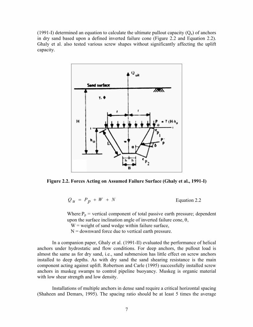
gonal pattern to measure a soil moisture profile throughout the test cell (Figures 3.6 and 3.7).
tion in water. As the soil warms, the moisture content returns to pre-freeze levels (Figure 3.15).
Compound
Four thermistors were installed in the test section, 40 mm (16 in) away from each pier,
and one in the center of the test section (Figure 3.6). The thermistor strings were positioned as close to the location of the piers as possible so they were not damaged when the piers were installed. The center thermistor was used to monitor temperature uniformity within the block of soil. Thermistor nodes were located at depths of 1,219 mm (48 in) and 1,829 mm (72 in) to correspond to the locations of the
Average daily thermistor data was plotted as shown in Figures 3.11 to 3.14. It was
assumed that the soil freezes at 0°C (32°F). Shortly after installation of Thermistor 3, the node at 1524 mm (60 in) gave unreasoc
Moisture Sensors: Fifteen Campbell soil moisture probes were installed in the test section. Three columns of five sensors were located in a dia
Hourly data was collected and the average daily water content reported. As the water in
the soil turns to ice, the probe interprets this change as a reduc
29

HELICAL PIER TEST SECTIONAVERAGE DAILY THERMISTER 1
-30
-20
-10
0
10
20
30
40
50
60
70
80
18-A
ug
25-A
ug
01-S
ep
08-S
ep
15-S
ep
22-S
ep
29-S
ep
06-O
ct
13-O
ct
20-O
ct
27-O
ct
03-N
ov
10-N
ov
17-N
ov
24-N
ov
01-D
ec
08-D
ec
15-D
ec
22-D
ec
29-D
ec
TEM
PER
ATU
RE
(F)
Surface 152 305 457 610 762 914 1067 12191372 1524 1676 1829 1981 2134 2286 2438
mm below surface
27
21
16
10
4
-1
-7
-12
-18
-23
-29
-34
TEMPER
ATU
RE (C
)
HELICAL PIER TEST SECTIONAVERAGE DAILY THERMISTER 1
0
10
20
30
40
50
01-J
an
08-J
an
15-J
an
22-J
an
29-J
an
05-F
eb
12-F
eb
19-F
eb
26-F
eb
04-M
ar
11-M
ar
18-M
ar
25-M
ar
01-A
pr
08-A
pr
15-A
pr
22-A
pr
29-A
pr
06-M
ay
13-M
ay
TEM
PER
ATU
RE
(F)
Surface 152 305 457 610 762 9141067 1219 1372 1524 1676 1829 19812134 2286 2438
mm below surface
10
4
-1
-7
-12
-18
TEMPER
ATU
RE (C
)
Figure 3.11. Average Daily Thermistor 1 Temperatures throughout Testing Period
30

HELICAL PIER TEST SECTIONAVERAGE DAILY THERMISTER 2
-30-20-10
01020304050607080
18-A
ug
25-A
ug
01-S
ep
08-S
ep
15-S
ep
22-S
ep
29-S
ep
06-O
ct
13-O
ct
20-O
ct
27-O
ct
03-N
ov
10-N
ov
17-N
ov
24-N
ov
01-D
ec
08-D
ec
15-D
ec
22-D
ec
29-D
ec
TEM
PER
ATU
RE
(F)
Surface 152 305 457 610 762 914 1067 12191372 1524 1676 1829 1981 2134 2286 2438
mm below surface
27211610 4 -1 -7 -12 -18 -23 -29 -34
TEMPER
ATU
RE (C
)
HELICAL PIER TEST SECTIONAVERAGE DAILY THERMISTER 2
0
10
20
30
40
50
01-J
an
08-J
an
15-J
an
22-J
an
29-J
an
05-F
eb
12-F
eb
19-F
eb
26-F
eb
04-M
ar
11-M
ar
18-M
ar
25-M
ar
01-A
pr
08-A
pr
TEM
PER
ATU
RE
(F)
Surface 6 12 18 24 30 36 42 4854 60 66 72 78 84 90 96
mm below surface
10
4
-1
-7
-12
-18
TEMPER
ATU
RE (C
)
Figure 3.12. Average Daily Thermistor 2 Temperatures throughout Testing Period
31

HELICAL PIER TEST SECTIONAVERAGE DAILY THERMISTER 3
-80
-60
-40
-20
0
20
40
60
80
18-A
ug
25-A
ug
1-Se
p
8-Se
p
15-S
ep
22-S
ep
29-S
ep
6-O
ct
13-O
ct
20-O
ct
27-O
ct
3-N
ov
10-N
ov
17-N
ov
24-N
ov
1-D
ec
8-D
ec
15-D
ec
22-D
ec
29-D
ec
TEM
PER
ATU
RE
(F)
surface 152 305 457 610 762 914 1067 12191372 1524 1676 1829 1981 2134 2286 2438
mm below surface
27
16
4
-7
-18
-29
-40
-51
-62
TEMPER
ATU
RE (C
)
HELICAL PIER TEST SECTIONAVERAGE DAILY THERMISTER 3
-80
-60
-40
-20
0
20
40
01-J
an
08-J
an
15-J
an
22-J
an
29-J
an
05-F
eb
12-F
eb
19-F
eb
26-F
eb
04-M
ar
11-M
ar
18-M
ar
25-M
ar
01-A
pr
08-A
pr
15-A
pr
22-A
pr
TEM
PER
ATU
RE
(F)
Surface 152 305 457 610 762 914 1067 12191372 1524 1676 1829 1981 2134 2286 2438
mm below surface
4
-7
-18
-29
-40
-51
-62
TEMPER
ATU
RE (C
)
Figure 3.13. Average Daily Thermistor 3 Temperatures throughout Testing Period
32

HELICAL PIER TEST SECTIONAVERAGE DAILY THERMISTER 4
-30-20-10
01020304050607080
18-A
ug
25-A
ug
01-S
ep
08-S
ep
15-S
ep
22-S
ep
29-S
ep
06-O
ct
13-O
ct
20-O
ct
27-O
ct
03-N
ov
10-N
ov
17-N
ov
24-N
ov
01-D
ec
08-D
ec
15-D
ec
22-D
ec
29-D
ec
TEM
PER
ATU
RE
(F)
Surface 152 305 457 610 762 914 1067 12191372 1524 1676 1829 1981 2134 2286 2438
mm below surface
27211610 4 -1 -7 -12 -18 -23 -29 -34
TEMPER
ATU
RE (C
)
HELICAL PIER TEST SECTIONAVERAGE DAILY THERMISTER 4
0
10
20
30
40
50
01-J
an
08-J
an
15-J
an
22-J
an
29-J
an
05-F
eb
12-F
eb
19-F
eb
26-F
eb
04-M
ar
11-M
ar
18-M
ar
25-M
ar
01-A
pr
08-A
pr
15-A
pr
22-A
pr
TEM
PER
ATU
RE
(F)
Surface 152 305 457 610 762 914 1067 12191372 1524 1676 1829 1981 2134 2286 2438
mm below surface
10
4
-1
-7
-12
-18
TEMPER
ATU
RE (C
)
Figure 3.14. Average Daily Thermistor 4 Temperatures throughout Testing Period
33

HELICAL PIER TEST SECTIONAVERAGE DAILY WATER CONTENT
0%
5%
10%
15%
20%
25%
30%
35%
40%
45%
50%
18-A
ug
25-A
ug
01-S
ep
08-S
ep
15-S
ep
22-S
ep
29-S
ep
06-O
ct
13-O
ct
20-O
ct
27-O
ct
03-N
ov
10-N
ov
17-N
ov
24-N
ov
01-D
ec
08-D
ec
15-D
ec
22-D
ec
29-D
ec
WA
TER
CO
NTE
NT
64 (A) 352 (A) 787 (A) 1248 (A) 1589 (A) 64 (B) 352 (B) 787 (B)1248 (B) 1589 (B) 64 (C) 352 (C) 787 (C) 1248 (C) 1589 (C)
mm below soil surface, () designates column
HELICAL PIER TEST SECTIONAVERAGE DAILY WATER CONTENT
0%
2%
4%
6%
8%
10%
12%
14%
01-J
an
08-J
an
15-J
an
22-J
an
29-J
an
05-F
eb
12-F
eb
19-F
eb
26-F
eb
04-M
ar
11-M
ar
18-M
ar
25-M
ar
01-A
pr
08-A
pr
15-A
pr
22-A
pr
29-A
pr
06-M
ay
13-M
ay
WA
TER
CO
NTE
NT
64 (A) 352 (A) 787 (A) 1248 (A) 1589 (A) 64 (B) 352 (B) 787 (B)1248 (B) 1589 (B) 64 (C) 352 (C) 787 (C) 1248 (C) 1589 (C)
mm below soil surface, () designates column
Figure 3.15 Average Daily Moisture Content throughout Testing Period
34

Creep Sensors: Pier settlement was measured using two devices. For vertical settlement the Banner Sonic OMNI-BEAM piezoelectric ultrasonic proximity sensors were used (Figure 3.16a). Any tilting of the piers was measured using the AccuStar II dual axis clinometer (Figure 3.16b).
Banner Sonic OMNI-BEAM: The operating range and temperature of the proximity
sensor is 100 – 660 mm (4 - 26 in) and between 0 to 50 °C (32 to 122 °F), respectively. It was noted during testing that while the sensor operated within the specified temperature range, there was an effect in the readings from the ambient air temperature. To correct for the fluctuations in temperature, a fourth stationary range sensor was used. Since the reference sensor’s location was fixed, the effects of temperature were corrected as a percent change from the reference distance.
To make sure that the OMNI-BEAM was reading the effects of the loading of the piers
and not moving with the piers, it was necessary to develop an independent system where the range readers were not attached to the steel plate (Figure 3.17). A reference beam system was constructed to hold the range readers. An aluminum collar 127 mm (5 in) in diameter was placed over each pier and bolts were tightened on each side of the pier to hold the collar in place (Figure 3.18). An aluminum plate 914 mm (36 in) long and 152 mm (6 in) wide was secured to the collar. These collars and plates were attached to the piers so that the end of the plate was located under the main reference beam and away from the center of the test section. It was the distance between this aluminum plate and the OMNI-BEAM device where vertical settlement was measured (Figure 3.19). The aluminum reference beams were secured to the framing on the north and south ends of the test section.
Figure 3.16a OMNI-BEAM Figure 3.16b AccuStar
35

Figure 3.17 Support System for OMNI-BEAM
Figure 3.18 Aluminum Collar Bolted to Sides of Pier
to Support Arm for Settlement Measurements
36

Figure 3.19 View from South End Showing Completed Test Cell
and Piers before Concrete Blocks are Loaded
AccuStar II dual axis clinometer: The tilt indicators operated over a range of ± 20 axial degrees. The operational temperature range is from –40 to +85 °C. The tilt indicators were placed on the aluminum arm, as close to the pier as possible (Figure 3.16b).
3.3.4 Pier Installation
Surface freezing of the test section began on August 18, 1999. After the freezing panels
were connected to the refrigeration system and leak tested, the temperatures of the sides and bottom panels was decreased to –1°C (30°F) and held until October 7. Over the next two days, the temperature was decreased again to -4°C (25°F) and then finally dropped to –18°C (0°F) to accelerate the freezing process through the test cell and reach a uniform temperature of -4°C (25°F).
On December 9, 1999 the surface freezing panels were removed for the installation of the
piers for a period of approximately 24 hours. All remaining freezing panels on the sides and bottom of the test section remained at a temperature of -4°C (25°F) during the installation. With the surface panels removed, the amount of thaw from the surface was less than 152 mm (6 in).
For the installation, the test section was cleaned off, the locations of the piers were
located and painted, and elevations shot on the three intended pier locations (Figure 3.6). The ambient temperature of the FERF was approximately 18 – 21°C (65 – 70°F) during the installation. Figure 3.8 shows the frozen test cell before the piers were installed.
37

The bottom helix for each pier was not to be less than 610 mm (24 in) above the geotextile to ensure that there was some soil for creeping under the pier. The geotextile was located at a depth of approximately 2.48 m (8.2 ft) below the soil surface. The length of the helix was 1.6 m (5.5 ft) and the length of the extension was 0.9 m (3.2 ft). The pier extensions were marked 635 mm (25 in) from the top, which would be the amount exposed above the surface.
According to Mr. Metlicka, the supervisor of the installation, the procedure used in the
FERF was similar to installations done in the field. A power auger mounted on a backhoe was used for the installation procedure (Figure 3.20). A double helix pier, designated as “Pier A”, located in the Northwest quadrant of the test section was installed first. Once the drill rig was set and the correct fitting for the top of the pier attached, the pier was set over the location and checked for vertical alignment. Then the pier was drilled down into the soil. During the installation of pier A, the 8,135 N⋅m (6,000 lb-ft) shear pins exceeded their maximum torque rating and broke. The pins were replaced with 10,846 Nm (8,000 lb-ft) shear pins that did not brake. This means that the installation torque was between 8 and 11 kNm (6000-8000 lb-ft). The pier extension was then secured to the top of the pier using a bolt and locking nut (Figure 3.21). Installation continued until 635 mm (25 in) of the pier extension was above the surface of the soil. Piers B and C were installed using the same procedure. After each pier was installed, the soil was leveled around the pier and water was poured around the extension.
After the installation, core samples were collected and the surface freezing panels were
replaced to refreeze the top soil. The panels were situated in such a way as to not interfere with the piers, but to still permit freezing. Thermal blankets were placed over any exposed surface to minimize temperature loss.
38

Figure 3.20 Pier Installation
Figure 3.21. Pier Extension is Attached
39
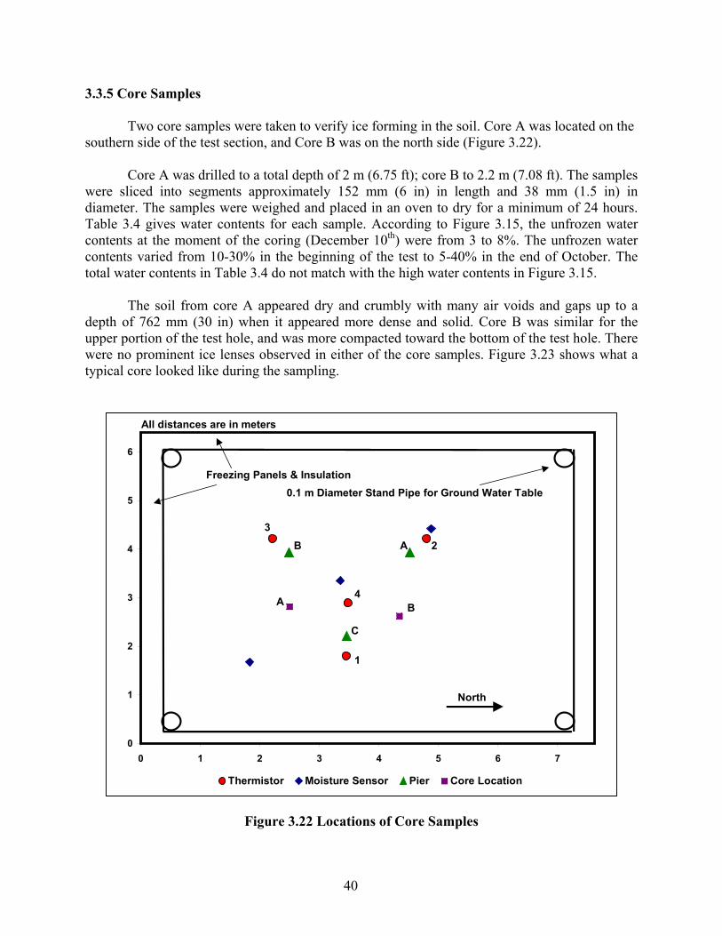
3.3.5 Core Samples Two core samples were taken to verify ice forming in the soil. Core A was located on the
southern side of the test section, and Core B was on the north side (Figure 3.22). Core A was drilled to a total depth of 2 m (6.75 ft); core B to 2.2 m (7.08 ft). The samples
were sliced into segments approximately 152 mm (6 in) in length and 38 mm (1.5 in) in diameter. The samples were weighed and placed in an oven to dry for a minimum of 24 hours. Table 3.4 gives water contents for each sample. According to Figure 3.15, the unfrozen water contents at the moment of the coring (December 10th) were from 3 to 8%. The unfrozen water contents varied from 10-30% in the beginning of the test to 5-40% in the end of October. The total water contents in Table 3.4 do not match with the high water contents in Figure 3.15.
The soil from core A appeared dry and crumbly with many air voids and gaps up to a
depth of 762 mm (30 in) when it appeared more dense and solid. Core B was similar for the upper portion of the test hole, and was more compacted toward the bottom of the test hole. There were no prominent ice lenses observed in either of the core samples. Figure 3.23 shows what a typical core looked like during the sampling.
0
1
2
3
4
5
6
0 1 2 3 4 5 6 7
Thermistor Moisture Sensor Pier Core Location
4
3 B
C
Freezing Panels & Insulation0.1 m Diameter Stand Pipe for Ground Water Table
North
All distances are in meters
A 2
1
A B
Figure 3.22 Locations of Core Samples
40

Table 3.4 Core Sample Water Contents
Core A Depth (mm)
Water Content (%)
Core B Depth (mm)
Water Content
(%)
Average Water
Content (%)
150 17.14 150 16.84 17.0 300 15.89 300 15.65 16.8 450 16.48 450 16.86 16.7 600 15.87 600 16.49 16.2 750 16.00 750 16.45 16.2 900 16.27 900 16.23 16.2 1050 16.64 1050 20.08 18.4 1200 16.66 1200 21.27 19.0 1350 14.59 1350 21.95 18.3 1500 16.03 1500 16.43 16.2 1650 13.83 1650 17.54 15.7 1800 18.28 1800 18.28 18.3 1950 16.90 1950 18.93 17.9
2100 23.12 23.1
Figure 3.23 Core Samples
41

3.3.6 Pier Loading After installing the piers and collecting the core samples, the freezing panels were
replaced on the surface to refreeze the top soil. A moisture barrier was placed between the soil surface and the freezing panels to prevent the soil from sticking to the panels. The panels did not touch the piers. Three sets of single panels were placed on the West side of the test cell around Piers A and B. Two sets of 5 panels (or a 5-pack) were placed on the East side of the test cell on either side of Pier C. The freezing panels were re-connected to the glycol refrigeration system and set to –4°C (25°F) to refreeze the soil surface. Thermal blankets were placed over any exposed surface to minimize temperature loss.
To ensure vertical loading, rounded endcaps were glued to the top of the piers with epoxy
and allowed to set for approximately 24 hours (Figure 3.24). Elevations of the piers with the endcaps were recorded.
Figure 3.24 Installed Pier with Endcap
Once the soil reached the desired temperature, a steel plate 2.4 m wide by 3 m long by
25.4 mm thick, and weighing 14.7 kN (8 ft wide by 10 ft long by 1 in thick, weighing 3,300 lbs) was loaded onto the piers. Lines were drawn on the plate to line up the piers as the plate was placed. Outlines of the blocks were also marked on the plate to minimize the amount of time needed to place the blocks. A crane was used to pick up each block and place it on the steel plate. To guide the block into position and disconnect each block from the crane, at least one person was needed to be standing on the steel plate. Given the current set up, it was not possible to load the piers using a fully automated system to capture the instant deformation when the pier was loaded. The OMNI-BEAM proximity sensors measured movement on the plate while the
42

blocks were placed. The blocks were loaded one at a time using configurations given in Table 3.5 for the both testing temperatures.
Table 3.5 Loading Configurations
Configuration Total Load (kN) Load per Pier (kN) Steel Plate 15.2 5.1 Single block placed in the center of the steel plate
33.0 11.0
Double block, stacked in center of steel plate
50.8 16.9
Single block over each pier 68.7 22.9 Double blocks, stacked over each pier 122.1 40.7
There was not much clearance between the antennas, where the OMNI-BEAM devices
were mounted, and the steel plate. Care was used not to hit the antennas while trying to place the blocks, since it was reflected in the data. Even so, the additional movement on the plate was read by the instrumentation and should not be used for analysis.
When changing the block configurations from the stacked blocks in the center, the top
block was moved and placed over Pier A. The bottom block was placed over Pier C and a third placed over Pier B. Moving and placing the blocks required some time, up to 30 minutes, to move everything into position and set it down. Figures 3.25 and 3.26 show the loaded piers with single blocks and double blocks.
After the blocks were set, data was collected for 24 hours. If no movement was observed
in the data, the blocks were moved into the next configuration. Just prior to placing the first block, the data collection system was started and it collected readings every 10 seconds during the first hour, every minute during the second hour and every 15 minutes for 22 hours. The following day, the data was reviewed for any settlement. Results from the data are given in the next section. Based on the data, concrete blocks were then added to load the piers and monitor the response.
43

Figure 3.25 Loading Piers with Three Concrete Blocks (view looking North)
Figure 3.26 Loading Piers with Six Concrete Blocks
3.4 Test Results 3.4.1 Test at –4°C
On December 16, 1999 the steel plate was set on the piers. Data was collected for 24 hours to see the response of the piers before the blocks were loaded. The output from the OMNI-BEAM sensors was in inches. As mentioned previously, these sensors measured the distance from the device to the aluminum arm. Table 3.6 gives the initial readings of the sensors.
44

Pier loading began the morning of December 17, 1999 when the single block was placed
in the center of the steel plate. Figure 3.27 shows the results of loading the single block. The spike seen after loading is believed to be from the change in temperature in the FERF when the South doors were opened and the outdoor temperature was much lower than that of the FERF. This was when a reference sensor was installed and the data was corrected for the effects of temperature. No changes were seen in the data and the second block was loaded on December 18, 1999 (Figure 3.28).
erature f the panels was increased to -1°C (30°F) to warm the soil for the next testing condition.
Table 3.6 Initial Readings of OMNI-BEAM Sensors
D Distance
On the morning of December 20, 1999 the blocks were moved, one over each pier. The
top block from the center stack, was placed on Pier A and the bottom block moved to Pier C. Pier B was loaded last with a third block. Again, the data suggest no settlement by the piers (Figure 3.29). Since there was no change in the data, the second layer of blocks was placed about an hour and a half later on December 20. Pier A was loaded first and the response was watched for a few minutes to check the stability of the plate. Pier A did show an increase in vertical distance after the block was loaded and then it leveled off. Pier C showed no change when loaded. Pier B (single helix) did show a small amount of change (Figures 3.30 and 3.31). No change was seen from any of the block configurations. The blocks stayed in position until December 21, 1999 when all of the blocks and the steel plate were removed. The blocks were removed from the piers in the same order as they were placed. After the blocks and plate were removed, elevations of the piers were taken. The piers showed no change in elevation, signifying no settlement during the test at -4°C. The test section remained dormant to see if there was any rebound by the now unloaded piers. The test concluded on January 3, 2000 and the tempo
istance(mm) (in)
Pier A 205.5 8.09 Pier B 222.8 8.77 Pier C 214.4 8.44
gle’ movement could be felt. As shown in the results, no changes in tilt occurred during the test.
Figures 3.31 through 3.38 show the readings for the tilt meters for the test at -4°C. For all piers, the X-direction shows movement in the East-West direction and the Y-direction shows movement in the North-South direction. The output values for the tilt meters were in millivolts (mV). A change of 56 mV is equivalent to 1 degree of axial movement. Each tilt meter was calibrated with 2,500 mV as dead center. Once the meters were set at each pier, the initial reading was used for the baseline to track any movement. Table 3.7 shows the initial tilt meter readings. The only movement registered by the tilt meters was caused during placement of the blocks. When someone stood on the plate to guide the block in place and right after placement of the block, a ‘wig
45

VERTICAL SETTLEMENTSingle Concrete Block in Center of Plate
8.0
8.1
8.2
8.3
8.4
8.5
8.6
8.7
8.8
8.9
9.0
12/1
7/99
6:0
0
12/1
7/99
8:2
4
12/1
7/99
10:
48
12/1
7/99
13:
12
12/1
7/99
15:
36
12/1
7/99
18:
00
12/1
7/99
20:
24
12/1
7/99
22:
48
12/1
8/99
1:1
2
INC
HES
PIER A PIER B PIER C
203
206
208
211
213
216
218
221
224
226
229M
ILLIMETER
S
Figure 3.27 Pier Settlement at -4°C with Concrete Block Placed in Center of Steel Plate
VERTICAL SETTLEMENTDouble Stack of Concrete Blocks in Center of Plate
8.0
8.1
8.2
8.3
8.4
8.5
8.6
8.7
8.8
8.9
9.0
12/1
8/99
6:2
8
12/1
8/99
6:4
3
12/1
8/99
6:5
7
12/1
8/99
7:1
2
12/1
8/99
7:2
6
12/1
8/99
7:4
0
12/1
8/99
7:5
5
12/1
8/99
8:0
9
12/1
8/99
8:2
4
INC
HES
PIER A PIER B PIER C
203
206
208
211
213
216
218
221
224
226
229
MILLIM
ETERS
Figure 3.28 Pier Settlement at -4°C with Two Concrete Blocks Placed in Center of Steel Plate
46
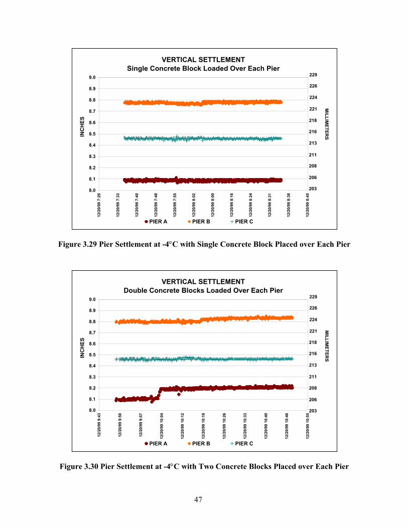
VERTICAL SETTLEMENTSingle Concrete Block Loaded Over Each Pier
8.0
8.1
8.2
8.3
8.4
8.5
8.6
8.7
8.8
8.9
9.0
12/2
0/99
7:2
6
12/2
0/99
7:3
3
12/2
0/99
7:4
0
12/2
0/99
7:4
8
12/2
0/99
7:5
5
12/2
0/99
8:0
2
12/2
0/99
8:0
9
12/2
0/99
8:1
6
12/2
0/99
8:2
4
12/2
0/99
8:3
1
12/2
0/99
8:3
8
12/2
0/99
8:4
5
INC
HES
PIER A PIER B PIER C
203
206
208
211
213
216
218
221
224
226
229M
ILLIMETER
S
Figure 3.29 Pier Settlement at -4°C with Single Concrete Block Placed over Each Pier
VERTICAL SETTLEMENTDouble Concrete Blocks Loaded Over Each Pier
8.0
8.1
8.2
8.3
8.4
8.5
8.6
8.7
8.8
8.9
9.0
12/2
0/99
9:4
3
12/2
0/99
9:5
0
12/2
0/99
9:5
7
12/2
0/99
10:
04
12/2
0/99
10:
12
12/2
0/99
10:
19
12/2
0/99
10:
26
12/2
0/99
10:
33
12/2
0/99
10:
40
12/2
0/99
10:
48
12/2
0/99
10:
55
INC
HES
PIER A PIER B PIER C
203
206
208
211
213
216
218
221
224
226
229
MILLIM
ETERS
Figure 3.30 Pier Settlement at -4°C with Two Concrete Blocks Placed over Each Pier
47

TILT X-DIRECTION (East - West)Single Concrete Block in Center of Plate
2360
2410
2460
2510
2560
12/1
7/99
6:0
0
12/1
7/99
8:2
4
12/1
7/99
10:
48
12/1
7/99
13:
12
12/1
7/99
15:
36
12/1
7/99
18:
00
12/1
7/99
20:
24
12/1
7/99
22:
48
12/1
8/99
1:1
2
mill
i Vol
ts
PIER A PIER B PIER C
Figure 3.31 Tilt Readings for X-Direction for Single Block in Center of Plate
TILT Y-DIRECTION (North-South)Single Concrete Block in Center of Plate
2360
2410
2460
2510
2560
12/1
7/99
6:0
0
12/1
7/99
8:2
4
12/1
7/99
10:
48
12/1
7/99
13:
12
12/1
7/99
15:
36
12/1
7/99
18:
00
12/1
7/99
20:
24
12/1
7/99
22:
48
12/1
8/99
1:1
2
mill
i Vol
ts
PIER A PIER B PIER C
Figure 3.32 Tilt Readings for Y-Direction for Single Block in Center of Plate
48

TILT X-DIRECTION (East - West)Double Stack of Concrete Blocks in Center of Plate
2360
2410
2460
2510
2560
12/1
8/99
6:2
8
12/1
8/99
6:4
3
12/1
8/99
6:5
7
12/1
8/99
7:1
2
12/1
8/99
7:2
6
12/1
8/99
7:4
0
12/1
8/99
7:5
5
12/1
8/99
8:0
9
12/1
8/99
8:2
4
mill
i Vol
ts
PIER A PIER B PIER C
Figure 3.33 Tilt Readings for X-Direction for Two Blocks in Center of Plate
TILT Y-DIRECTION (North-South)Double Stack of Concrete Blocks in Center of Plate
2360
2410
2460
2510
2560
12/1
8/99
6:2
8
12/1
8/99
6:4
3
12/1
8/99
6:5
7
12/1
8/99
7:1
2
12/1
8/99
7:2
6
12/1
8/99
7:4
0
12/1
8/99
7:5
5
12/1
8/99
8:0
9
12/1
8/99
8:2
4
mill
i Vol
ts
PIER A PIER B PIER C
Figure 3.34 Tilt Readings for Y-Direction for Two Blocks in Center of Plate
49

TILT X-DIRECTION (East - West)Single Concrete Block Loaded Over Each Pier
2360
2410
2460
2510
2560
12/2
0/99
7:2
6
12/2
0/99
7:3
3
12/2
0/99
7:4
0
12/2
0/99
7:4
8
12/2
0/99
7:5
5
12/2
0/99
8:0
2
12/2
0/99
8:0
9
12/2
0/99
8:1
6
12/2
0/99
8:2
4
12/2
0/99
8:3
1
12/2
0/99
8:3
8
12/2
0/99
8:4
5
mill
i Vol
ts
PIER A PIER B PIER C
Figure 3.35 Tilt Readings for X-Direction for Single Block over Each Pier
TILT Y-DIRECTION (North-South)Single Concrete Block Loaded Over Each Pier
2360
2410
2460
2510
2560
12/2
0/99
7:2
6
12/2
0/99
7:3
3
12/2
0/99
7:4
0
12/2
0/99
7:4
8
12/2
0/99
7:5
5
12/2
0/99
8:0
2
12/2
0/99
8:0
9
12/2
0/99
8:1
6
12/2
0/99
8:2
4
12/2
0/99
8:3
1
12/2
0/99
8:3
8
12/2
0/99
8:4
5
mill
i Vol
ts
PIER A PIER B PIER C
Figure 3.36 Tilt Readings for Y-Direction for Single Block over Each Pier
50

TILT X-DIRECTION (East - West)Double Concrete Blocks Loaded Over Each Pier
2360
2410
2460
2510
2560
12/2
0/99
9:4
3
12/2
0/99
9:5
0
12/2
0/99
9:5
7
12/2
0/99
10:
04
12/2
0/99
10:
12
12/2
0/99
10:
19
12/2
0/99
10:
26
12/2
0/99
10:
33
12/2
0/99
10:
40
12/2
0/99
10:
48
12/2
0/99
10:
55
mill
i Vol
ts
PIER A PIER B PIER C
Figure 3.37 Tilt Readings for X-Direction for Two Blocks over Each Pier
TILT Y-DIRECTION (North-South)Double Concrete Blocks Loaded Over Each Pier
2360
2410
2460
2510
2560
12/2
0/99
9:4
3
12/2
0/99
9:5
0
12/2
0/99
9:5
7
12/2
0/99
10:
04
12/2
0/99
10:
12
12/2
0/99
10:
19
12/2
0/99
10:
26
12/2
0/99
10:
33
12/2
0/99
10:
40
12/2
0/99
10:
48
12/2
0/99
10:
55
mill
i Vol
ts
PIER A PIER B PIER C
Figure 3.38 Tilt Readings for Y-Direction for Two Blocks over Each Pier
51

Table 3.7. Initial Tilt Meter Readings at Start of Test
Pier Location X (mV)
Y (mV)
A 2,419 2,537 B 1,889 2,824 C 2,419 2,362
3.4.2 Test at –1°C
Beginning January 3, 2000 the temperatures of the panels were increased to -1°C (30°F) to warm the soil throughout the test cell. The thermistor temperatures were monitored regularly until a uniform soil temperature of approximately -1°C (30°F) was achieved. On March 7, 2000 the “warm frozen ground testing” procedure began using the same sequence as the test at –4°C. The loading portion of the test concluded on May 8, 2000 with the removal of all blocks and the steel plate. The data collection system continued to monitor the readings overnight. No further changes were seen in the data, and the test was discontinued.
While loading the steel plate on March 6, 2000, it came in contact with Pier C, causing it to tilt slightly, by less than 12.5 mm (0.5 in). An attempt was made to straighten the pier while the plate was placed, but the pier moved back out of alignment.
On March 9, 2000 the single center block was placed on the steel plate (Figure 3.39). The
data suggested some movement in Pier C, so the test continued until March 13, when it appeared that any movement had stopped and the second block was stacked on top of the first (Figure 3.40). This block arrangement was held until April 5, when the settlement stabilized. Then the single blocks were placed over each pier. When no change was evident in the data, the second layer of blocks was added on April 7 (Figures 3.41 and 3.42). The piers remained this way until May 5, when all blocks and the steel plate were removed from the piers. The data collection system continued to monitor the piers for any rebound. No rebound was present in the data and the test was discontinued.
Results from the tilt meters are given in Figures 3.43 to 3.50. Both measurements in
distance and tilt show some activity during the testing. For example Figure 3.42 shows pier A and B moving up 6 and 4 mm (0.24 and 0.16 in) respectively and pier C moving down 5 mm (0.20 in), which does not make sense regarding creep. The tilting of the piers was less than 56mV that is less than one degree.
52

VERTICAL SETTLEMENTSingle Concrete Block in Center of Plate
8.0
8.1
8.2
8.3
8.4
8.5
8.6
8.7
8.8
8.9
9.0
03/0
9/20
00 0
:00
03/0
9/20
00 1
2:00
03/1
0/20
00 0
:00
03/1
0/20
00 1
2:00
03/1
1/20
00 0
:00
03/1
1/20
00 1
2:00
03/1
2/20
00 0
:00
03/1
2/20
00 1
2:00
03/1
3/20
00 0
:00
03/1
3/20
00 1
2:00
03/1
4/20
00 0
:00
INC
HES
PIER A PIER B PIER C
203
206
208
211
213
216
218
221
224
226
229M
ILLIMETER
S
Figure 3.39 Pier Settlement at -1°C with Concrete Block in Center of Steel Plate
VERTICAL SETTLEMENTDouble Stack of Concrete Blocks in Center of Plate
8.0
8.1
8.2
8.3
8.4
8.5
8.6
8.7
8.8
8.9
9.0
12/1
8/99
6:2
8
12/1
8/99
6:4
3
12/1
8/99
6:5
7
12/1
8/99
7:1
2
12/1
8/99
7:2
6
12/1
8/99
7:4
0
12/1
8/99
7:5
5
12/1
8/99
8:0
9
12/1
8/99
8:2
4
INC
HES
PIER A PIER B PIER C
203
206
208
211
213
216
218
221
224
226
229
MILLIM
ETERS
Figure 3.40 Pier Settlement at -1°C with Two Concrete Blocks in Center of Steel Plate
53

VERTICAL SETTLEMENTSingle Concrete Blocks Loaded Over Each Pier
8.0
8.2
8.4
8.6
8.8
9.0
9.2
04/0
5/20
00 0
:00
04/0
5/20
00 1
2:00
04/0
6/20
00 0
:00
04/0
6/20
00 1
2:00
04/0
7/20
00 0
:00
04/0
7/20
00 1
2:00
INC
HES
PIER A PIER B PIER C
203
208
213
218
224
234
229
MILLIM
ETERS
Figure 3.41 Pier Settlement at -1°C with Concrete Block Placed over Each Pier
VERTICAL SETTLEMENTDouble Concrete Blocks Loaded Over Each Pier
7.8
8.0
8.2
8.4
8.6
8.8
9.0
9.2
9.4
04/0
4/20
00 0
:00
04/0
9/20
00 0
:00
04/1
4/20
00 0
:00
04/1
9/20
00 0
:00
04/2
4/20
00 0
:00
04/2
9/20
00 0
:00
05/0
4/20
00 0
:00
05/0
9/20
00 0
:00
INC
HES
PIER A PIER B PIER C
203
208
213
218
224
234
229
MILLIM
ETERS
198
239
Figure 3.42 Pier Settlement at -1°C with Two Concrete Blocks Placed over Each Pier
54

TILT X-DIRECTION (East - West)Single Concrete Block in Center of Plate
2360
2410
2460
2510
2560
12/1
7/99
6:0
0
12/1
7/99
8:2
4
12/1
7/99
10:
48
12/1
7/99
13:
12
12/1
7/99
15:
36
12/1
7/99
18:
00
12/1
7/99
20:
24
12/1
7/99
22:
48
12/1
8/99
1:1
2
mill
i Vol
ts
PIER A PIER B PIER C
Figure 3.43 Tilt Readings for X-Direction for Single Block in Center of Plate
TILT X-DIRECTION (East - West)Single Concrete Block in Center of Plate
2360
2410
2460
2510
2560
12/1
7/99
6:0
0
12/1
7/99
8:2
4
12/1
7/99
10:
48
12/1
7/99
13:
12
12/1
7/99
15:
36
12/1
7/99
18:
00
12/1
7/99
20:
24
12/1
7/99
22:
48
12/1
8/99
1:1
2
mill
i Vol
ts
PIER A PIER B PIER C
Figure 3.44 Tilt Readings for Y-Direction for Single Block in Center of Plate
55

TILT X-DIRECTION (East - West)Double Concrete Blocks in Center of Plate
2360
2410
2460
2510
2560
03/1
0/20
00 0
:00
03/1
5/20
00 0
:00
03/2
0/20
00 0
:00
03/2
5/20
00 0
:00
03/3
0/20
00 0
:00
04/0
4/20
00 0
:00
04/0
9/20
00 0
:00
mill
i Vol
ts
PIER A PIER B PIER C
Figure 3.45 Tilt Readings for X-Direction for Two Blocks in Center of Plate
TILT Y-DIRECTION (North-South)Double Concrete Blocks in Center of Plate
2360
2410
2460
2510
2560
03/1
0/20
00 0
:00
03/1
5/20
00 0
:00
03/2
0/20
00 0
:00
03/2
5/20
00 0
:00
03/3
0/20
00 0
:00
04/0
4/20
00 0
:00
04/0
9/20
00 0
:00
mill
i Vol
ts
PIER A PIER B PIER C
Figure 3.46 Tilt Readings for Y-Direction for Two Blocks in Center of Plate
56

TILT X-DIRECTION (East - West)Single Concrete Block Loaded Over Each Pier
2360
2410
2460
2510
2560
04/0
5/20
00 0
:00
04/0
5/20
00 1
2:00
04/0
6/20
00 0
:00
04/0
6/20
00 1
2:00
04/0
7/20
00 0
:00
04/0
7/20
00 1
2:00
mill
i Vol
ts
PIER A PIER B PIER C
Figure 3.47 Tilt Readings for X-Direction for Single Block over Each Pier
TILT Y-DIRECTION (North-South)Single Concrete Block Loaded Over Each Pier
2360
2410
2460
2510
2560
04/0
5/20
00 0
:00
04/0
5/20
00 1
2:00
04/0
6/20
00 0
:00
04/0
6/20
00 1
2:00
04/0
7/20
00 0
:00
04/0
7/20
00 1
2:00
mill
i Vol
ts
PIER A PIER B PIER C
Figure 3.48 Tilt Readings for Y-Direction for Single Block over Each Pier
57

TILT X-DIRECTION (East - West)Double Concrete Blocks Loaded Over Each Pier
2360
2410
2460
2510
2560
04/0
4/20
00 0
:00
04/0
9/20
00 0
:00
04/1
4/20
00 0
:00
04/1
9/20
00 0
:00
04/2
4/20
00 0
:00
04/2
9/20
00 0
:00
05/0
4/20
00 0
:00
05/0
9/20
00 0
:00
mill
i Vol
ts
PIER A PIER B PIER C
Figure 3.49 Tilt Readings for X-Direction for Two Blocks over Each Pier
TILT Y-DIRECTION (North-South)Double Concrete Blocks Loaded Over Each Pier
2360
2410
2460
2510
2560
04/0
4/20
00 0
:00
04/0
9/20
00 0
:00
04/1
4/20
00 0
:00
04/1
9/20
00 0
:00
04/2
4/20
00 0
:00
04/2
9/20
00 0
:00
05/0
4/20
00 0
:00
05/0
9/20
00 0
:00
mill
i Vol
ts
PIER A PIER B PIER C
Figure 3.50 Tilt Readings for Y-Direction for Two Blocks over Each Pier
58

3.5 Conclusions for CRREL Experiment The following conclusions were drawn from the FERF experiment:
• The piers did not settle or tilt at -4°C. • The results for the -1°C test indicated some movement, which may be the result of uneven
temperatures on the soil basin and partial thaw settlement. The vertical movement of piers was in order of a few millimeters up and down and the piers tilted less than one degree.
• The FEA models could not be calibrated using the test results, because of the uneven temperatures in the test cell and the short loading times.
• Installation of the piers in the frozen ground proceeded without any problems. 3.6 References for CRREL Experiment AccuStar II Dual Axis Clinometer, Operating Instructions and Installation Information, North American Operations, Lucas Control Systems, 1000 Lucas Way, Hampton, VA 23666. U.S. Army Corps of Engineers, 1997, Technical Instructions: Airfield Pavement Evaluation, TI 826-01, Engineering Division, Washington D.C. Sonic OMNI-BEAM, Banner Engineering Corp., 9714 10th Avenue No., Minneapolis, MN 55441.
59

4. FIELD STUDY 4.1 Introduction
Helical pier installations have become very common in the past few years in permafrost construction. As their effectiveness, particularly in ice-rich areas, has been demonstrated their utilization has become routine.
Table 4.1 lists examples of some of the helical pier installations in permafrost in “Bush Alaska” in the past few years. Piers have been used as foundations in frozen ground for a variety of construction projects, boardwalks, fences, utilidors, and arctic pipe. As evident from Table 4.1, thousands of helical piers are currently installed in Alaska. The primary sources for this field information are the State of Alaska Department of Environmental Conservation Village Safe Water (VSW) and the Alaska Native Tribal Health Consortium, Department of Environmental Health and Engineering (ANTHC, DEHE).
Table 4.1 Examples of Helical Pier Installations in Rural Alaska
Year Location Comments
1996 Kiana Fence installation, pilot hole and backhoe, Chance piers
1998 Selawik Fence, 1,224 Dixie brand piers
Noorvik Arctic pipe installation, 500 piers
1999 Selawik Fence, 2,400 piers
Tuntutuliak Boardwalk to sewage lagoon
2000 Chignik Fence around lagoon, 24 piers, not a permafrost area
2001 Eek Planned sewage lagoon fence, 180 piers
Selawik Arctic pipe and service lines to homes, 500
piers
2000/2001 Chefornak Boardwalk, summer installation with skid loader
60

4.2. Installations
Helical piers can be installed any time of year. Installation is usually easier in the fall when the ground is frozen before significant snow buildup. Summer installation in wet areas can be challenging due to the soft ground and surface water. Installation in wet areas can be conducted with ground mats and proper selection of the installation equipment.
Piers are installed by auguring them into the ground. Typically, a backhoe or skid loader is used with a rotating power head. The rotating head can be a specially designed tool or can be made by modifying an existing rotating head. The amount of vertical force necessary depends upon the soil conditions and the temperature of the permafrost and must determined in the field by the installer. Colder, rockier soils require more pressure to be applied to the pier as it is augured.
Neither VSW nor ANTHC drill pilot holes for the piers. For some of the first pier
installations pilot holes were air-drilled to ensure that the piers would be straight and plumb. Installers have found that piers can be installed correctly without pilot holes (Dixon, 2001).
Design factors typically used are relatively simple. Besides load determination the critical
factor is the depth of the active layer. If the pier helix is founded well below the active layer a solid, long lasting foundation is almost certain. The diameter of the steel rod portion of the pier is too small to provide enough surface area for heaving soils to lift the pier. Therefore, piers remain in place without any displacement or jacking.
Utilidors and arctic pipe are traditionally installed on grade or on posts with a short life
expectancy. Heat loss from on-grade utilidors melts the permafrost within a few years causing displacement of the utilities that often makes them unusable. Figure 4.1 and Figure 4.2 show typical on-grade utilidors. Posts also perform poorly in frozen ground because of jacking. Therefore, the VSW and ANTHC prefer helical piers as foundations for gravity and vacuum sewage lines in arctic pipe. Grade is critical for these sewage lines and helical piers have provided a long-lasting, stable foundation in cold, ice-rich permafrost without requiring adjustment.
More and more helical piers are used for non-frost jacking fence post anchors. They have
higher initial cost than posts with lateral supports laid on grade, but the longer service life and reduced maintenance operations makes them an economical foundation. The use of helical piers could revolutionize housing foundations in permafrost as well as seasonal frost areas. The characteristics, such as ease and speed of installation, no curing time and no frost jacking make helical piers very attractive foundations and it is only a question of time when they full potential is realized.
61

Figure 4.1 Utilidor on Grade in Permafrost Area, Noorvik, Alaska (ANTHC, DEHE)
Figure 4.2 Damaged Utilidor on Grade, Noorvik, Alaska (ANTHC, DEHE)
62

4.3 Field Applications
ANTHC has utilized helical piers in numerous installations throughout rural Alaska. Examples in this report are in the villages of Noorvik, Kiana, and Selawik in northwest Alaska near Kotzebue Sound where permafrost is continuous and considered cold. These villages can be located on the map in Figure 4.3.
Figure 4.3 Location of Villages in State of Alaska (Grolier Encyclopedia, 2001)
Helical piers are the foundation for the arctic pipe installation in Noorvik. Originally, the sewage pipes were in a utilidor on grade. Noorvik is in a very ice-rich permafrost area, 50 to 400% ice, and the on-grade installation caused severe thaw subsidence and chronic malfunctions of the vacuum sewage line. In 1998, new arctic pipe was installed using helical piers with tremendous success. The grade-sensitive sewage vacuum system has operated as designed. Photos of the installation at Noorvik are shown in Figure 4.4 and Figure 4.5. Figure 4.6 is the finished utilidor installation in Noorvik.
63

Figure 4.4 Helical Piers in Noorvik, Alaska Installed as Foundations for Arctic Pipe Sewage Installation.
The Arctic Pipe Contains a Vacuum Sewage Line. (ANTHC, DEHE)
Figure 4.5 Arctic Pipe with Helical Piers as a Foundation in Noorvik, Alaska (ANTHC, DEHE)
64

Figure 4.6 Finished Utilidor on Helical Piers in Noorvik, Alaska (ANTHC, DEHE)
Typical installations consist of a 1.68 m (5.5 ft) pier with a 2.13 m (7 ft) extension. The active layer in the Noorvik area is about 0.6 m (2 ft) thick and this pier length has proven to be adequate to firmly anchor in the permafrost. The pier is screwed in until a stub is left at the surface and the post or tubing that is necessary for the construction is bolted to the stub. Figure 4.7 and Figure 4.8 are the details for typical pier installation and supports. These designs were used in Noorvik.
65

Figure 4.7 Typical Pier Detail (ANTHC, DEHE)
66

Figure 4.8 Typical Detail for Helical Piers as Used in Noorvik for the Utilidor and Arctic Pipe Installation (ANTHC, DEHE)
67

The village of Kiana is built on cold, ice-rich permafrost. An extensive fence project was built in 1996 using helical piers as the foundation for the posts. As of this writing (December, 2001) the piers remain straight and plumb. The fence is shown in Figure 4.9 in a photo taken in 1998. The installation for the fence piers are the same as for the utilidors with line or corner posts bolted to the pier shafts.
Figure 4.9 Fence Constructed in Kiana in 1996 (ANTHC, DEHE)
VSW has projects in several villages in the Kuskokwim Delta. Permafrost in this area is warm and discontinuous. Pier installations have been very successful when compared to traditional techniques. But, because of the nature of the discontinuous permafrost and variations in the depth of the active layer there are more instances of jacking or heave of the piers.
In Chefornak, helical piers were used to construct a boardwalk during summer. A skid
loader with a drive head installed the piers while advancing along the boardwalk as it was constructed. Construction advanced across the swampy area in 1.8 m (6 ft) segments (Menough, 2001). The boardwalk in Chefornak will have piers replaced in the next year; they were not installed deeply enough. Inconsistent soils and thus a great variation in active layer depth in the area are the likely cause of the problem. Figure 4.10 and Figure 4.11 show the installation of the Chefornak boardwalk.
68

Figure 4.10 The Summer Installation of the Boardwalk in Chefornak. (VSW) The Power Head on the Skid Loader Used to Install the Piers can be seen at the Right.
Figure 4.11 Installation of the Boardwalk in Chefornak (VSW)
69

In the village of Tuntutuliak helical piers are the foundation for a boardwalk. Tuntutuliak is subject to fall flooding caused by tidal surges with high winds. The boardwalk itself has not endured the flooding well. The piers have been very stable with the exception of a few located in the transition area between the permafrost soils and a lagoon. In that area the piers were not installed deeply enough. The active layer thickness is much greater in the area closer to the lagoon (Burleigh, 2001). 4.4 Conclusions for Field Study
Helical piers have been used in a variety of projects in frozen ground in rural areas of Alaska. They have been successful when installed deep enough below the active layer into the permafrost. They have carried the applied loads without failures and resisted the forces of heaving and jacking.
Installation of helical piers is more expensive than installation of utilities on grade or on
posts. However, since these traditionally used methods are simply not working, the long-term performance of helical piers justifies the expense, particularly, for grade-sensitive structures (Dixon, 2001). 4.5 References for Field Study Burleigh, Roger, November 2001, Interview, State of Alaska DEC-VSW. Dixon, Matthew, November 2001, Interview, ANTHC. Grolier Encyclopedia, 2001, Multimedia Encyclopedia Deluxe Edition, Scholastic. Menough, Jon, December 2001, Interview, State of Alaska DEC- VSW. Schubert, Dan, November 2001, Interview, GV Jones & Associates.
70

5. DEVELOPMENT OF FINITE ELEMENT MODEL 5.1 Introduction
Helical piers come in different types and shapes. Typical configurations of helical piers are shown in Figure 5.1. Current design methods for determining the capacity of helical piers are based upon very simple formulas that assume uniform stress distribution on helixes (Figure 5.1). These formulas may or may not be conservative (Equation 2.1, Figure 2.1). Some research has been conducted to describe the overall capacity and displacement of helical piers subjected to vertical and lateral loading (Narasimha Rao and Prasad, 1993, Prasad and Narasimha Rao, 1996, and Ghaly et al., 1991). Much less has been done to examine the distribution of stresses in the soil surrounding these piers, their behavior under prolonged loading in frozen ground, or the stresses within a typical helical pier during installation or under normal working loads.
Figure 5.1. Simplified Distribution of Bearing Pressure (A. B. Chance Co. 1996)
The purpose of developing Finite Element Analysis (FEA) models is to investigate the
behavior of helical pier foundations in frozen ground. Problems related to frozen ground include the risk that the piers will break during the installation, instantaneous strength, stability failure, and long-term creep failure in the frozen ground.
The complex geometry of helical piers is modeled precisely. Four objectives were
established to complete this study: 1) Analyze displacement and stress distribution in frozen soil due to an axial load
(instantaneous failure mode),
71

2) Analyze the stresses within the pier structure when it is subjected to this load, (instantaneous failure mode),
3) Provide a detailed analysis of the stresses within the pier during installation
(installation failure mode),
4) Investigate long-term creep settlement behavior in frozen ground (excessive settlement failure mode).
A FEA program, called ANSYS, was chosen to model all four of these situations for its
ability to model complex, nonlinear, three-dimensional conditions. The following four components were needed to do this:
1) Large Model: This model will analyze the soil stresses and displacements
immediately after the pier is subjected to its design load. This data is also critical for the development of more detailed analysis using sub-modeling techniques.
2) Small Model: The small model is a sub-model of the large model. It will analyze the stresses developed within the spiral structure by using results from the large model analysis.
3) Installation Failure Model: A detailed model of the spiral structure subjected to a
torsional load during installation will provide insight into the failure mechanism of helical piers during construction.
4) Creep Model: Creep analysis will be conducted to determine the long-term
displacement and soil stress in frozen ground. The FEA program ANSYS provides a variety of functions and features for modeling of
complicated conditions. However, little data exists for the displacement of helical piers and the surrounding soil when subjected to axial compressive loads. Therefore, it was planned that these results would be compared with physical tests to be conducted at the U.S. Army Corps of Engineers Cold Regions Research and Engineering Laboratory (CRREL) in Hanover, New Hampshire. The analysis results will be used to develop installation guidelines, and to create design curves for frozen ground in the future design work. 5.2 Basic Assumptions for Finite Element Analysis
The following sections describe the needed material properties and basic assumptions used in the analysis. 5.2.1 Geometric Considerations
The three-dimensional elements consist of several parts, a cylindrical soil column, a circular steel plate that represents the pier itself, and finally a steel pipe that represents the shaft
72

from the pier to the top of the soil. A three-dimensional analysis was chosen because it allows the general results to be applied to a sub-model with more specific geometry.
In the Large Model and the Creep Model a cylinder-shaped column of soil was chosen
because it is the easiest volume of soil to model in a cylindrical coordinate system. Based on the Theory of Elasticity, the physical size of the soil column was based on the vertical stress distribution under the center a circular plate. Since the soil column cannot be modeled as an infinite space, such as the actual Earth, the model was designed to allow the stress in the soil to fully develop with stress distribution at the bottom of the volume being less the 1% of the assumed uniform distributed pressure beneath the helix. This guarantees that the fixed boundary conditions at the bottom of the model will have a negligible effect on results. Thus for a 203 mm (8 in) diameter helix, a soil minimum depth of 1,245 mm (49 in) is required under the pier to achieve desired stress, strain and deformation levels. However, to further guarantee no interference from the boundaries a depth of 2,286 mm (90 in) was selected. This resulted in a theoretical maximum vertical stress only 0.30% of the assumed uniform distributed pressure beneath the helix. Furthermore, the additional depth helped create a convenient geometric expansion of the model element sizes. The 1,626 mm (64 in) diameter of the cylinder was established in a similar manner. A steel circular plate was chosen over an actual helix because the general behavior is the same and a circular plate saves considerable time in model development and actual analysis time. Also, steel pipe models the actual load-bearing element, and is used to transmit the load from the soil surface to the pier. 5.2.2 Frozen Soil Material Properties and Yield Criteria
In addition to the geometry of the model, physical properties of the soil had to be included in the model. A basic elastic-plastic model is used to represent the response of frozen soil. The frozen-soil parameters used in the model development are given in Table 5.1.
Table 5.1. Soil Parameters Used for Development of Models
Youngs Modulus MPa 1,800
ksi 261 Poisson’s Ratio 0.35
Unit Weight kN/m3 20 pcf 130
Friction Angle 20 Cohesion kPa 34.5
psi 5
The program used allows for numerous methods for non-linear analysis. The Drucker-
Prager yield criterion was used to describe the yield surface for the soil elements and to most accurately model the three-dimensional elastic-plastic properties of the soil. The Drucker-Prager criterion is preferred because it accounts for internal friction angle as well as cohesion, which allows hydrostatic stress to have an influence on yielding using the outer cone approximation to the Mohr-Coulomb law. The criterion creates a yield surface for the principal stresses within the
73
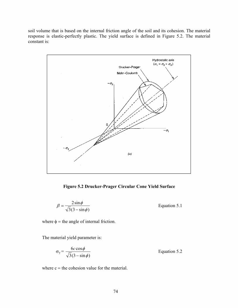
soil volume that is based on the internal friction angle of the soil and its cohesion. The material response is elastic-perfectly plastic. The yield surface is defined in Figure 5.2. The material constant is:
where
The m
wher
Figure 5.2 Drucker-Prager Circular Cone Yield Surface
)sin3(3sin2
φφβ
−= Equation 5.1
φ = the angle of internal friction.
aterial yield parameter is:
σy = )sin3(3
cos6φ
φ−
c Equation 5.2
e c = the cohesion value for the material.
74

The yield criterion is:
} [ ] }{{ 0213
21
=−
+= y
Tm sMsF σβσ Equation 5.3
where{ the deviator stresses, } =s
( )zyxm σσσσ ++=31
, and Equation 5.4
[M]= a constant scalar matrix.
5.2.3 Steel Material Properties and Yield Criteria
The spiral and central column were modeled using the material properties for steel - Bilinear Isotropic yield criteria. Figure 5.3 shows the concept of the material model. When stress in steel is lower than the yield level, the behavior of steel is linearly elastic. The bi-linear isotropic yield criteria are for the plastic behavior when stresses in steel reach the yield level. In the FEA models, the following parameters were used for the bi-linear yield surface:
σy = 345 MPa (50 ksi) E = 200,000 MPa (29,000 ksi) Et = 10,000 MPa (1,450 ksi) A typical geometry chosen for a pier includes a 76 mm (3 in) outer diameter pipe section
with 13 mm (0.5 in) wall thickness for the pipe; and a 254 mm (10 in) diameter, 13 mm (0.5 in) thick plate for the spiral. In the Large and Creep Model, the spirals were modeled using flat plates, which did not account for any pitch that would be present in the actual conditions. This was done to limit the overall number of elements in the large models and to simplify model construction. The effect of pitch was assumed to be negligible in determining the overall capacity of a pier. The element and material properties used in these models appear in Table 5.2.
Table 5.2. Pier Properties and FEA Parameters
Material E (MPa) ν ρ (kN/m3) Element Type Nodal DOF Steel shaft 200,000 0.3 77.0 Beam 6 Steel plate 200,000 0.3 77.0 Shell 6
75

Figure 5.3 Bi-linear Isotropic Material Non-linearity
5.2.4 Creep Formula and Parameters
To analyze the effects of creep, a creep formula was used with the addition of creep
parameters to simulate secondary creep effects over a period of time. The creep equations were determined based on previous research by Ladanyi and Johnston (Johnston and Ladanyi, 1974; Ladanyi and Johnston, 1974; and Ladanyi, 1983), and were selected to provide an upper bound for creep effects. The creep formula is as follows:
n
cu
ece
=
θσσ
εε && Equation 5.5
Where: eε& = reference strain rate, n = creep parameter, σe = equivalent stress, σcuθ = creep modulus corresponding the reference strain rate.
76

5.3 Sample Analyses on Stress, Strain and Deformation for Helix and Soil
The following sections contain examples of the work to describe how the analysis was conducted.
5.3.1 Soil Stress-Strain and Deformation Analyses – Large Model
Two large-scale models were created using a cylindrical volume of soil with a helical pier at the center: 1) Test Model to simulate the testing conditions at the CRREL, and 2) Deep Model to simulate conditions in the field. The soil cylinder of the Test Model had an overall diameter of 1,270 mm (50 in) and an overall depth of 3,048 mm (120 in). The Deep Model was used to investigate the effects of boundary interactions within the model. In this model the diameter remained 1,270 mm (50 in), but the depth was extended to 5,588 mm (220 in). In both models, the pier’s total embedded depth was 2,286mm (90 in) and each had two 254 mm (10 in) diameter helices spaced 762 mm (30 in) apart.
The geometry chosen for the pier includes an 89 mm (3½ in) outer diameter pipe section
with 13 mm (½ in) wall thickness for the shaft; and a 254 mm (10 in) diameter, 13 mm (½ in) thick plate for the spiral. For this large-scale model, the spirals were modeled using flat plates. This was done in order to limit the overall number of elements in the model.
Figure 5.4 shows the geometry of the Test Model (Figures a and b are given in different
scales for convenient viewing). A three-dimensional brick element was used to represent soil. The FEA mesh was carefully designed to keep all bricks in good shape/aspect ratio, and to provide reasonable connection with soil model while granting efficient computational time.
(a) FEA Model of Helical Piers (b) FEA Model of Soil Volume
Figure 5.4 FEA Meshes for Helical Piers and Soil Volume (not in same scale)
77

Boundary conditions for Test and Deep Models included translational restraint in the
horizontal directions for the sides of the soil cylinder and full restraint for the bottom of the soil cylinder.
Figure 5.5 shows the vertical soil displacement from the sample calculation for the Test
Model due to an ultimate axial load of 89 kN (20 kip). It is clear that the vertical displacement is concentrated near the pier. A relatively small vertical displacement can be attributed to the effects from shallow boundary conditions. The maximum displacement was 69 mm (2.72 in) which occurred in the soil around the helical pier.
Figure 5.5 Vertical Displacement in Soil for Shallow Model Due to Axial Load 89 kN (20 kip)
Figure 5.6 shows the vertical soil stress for Test Model under an ultimate axial load of 89
kN (20 kip). Small vertical tension stresses were developed above both plates with magnitudes up to 27 kPa (4 psi). These stresses are consistent with adhesion between the soil and the pipe or plate elements in this region and were limited by the Drucker-Prager yield criteria. The soil displacement due to the applied load and soil self-weight was greatest at points near the pier as would be expected. The small cohesion strength used in this model limited the ability of the soil elements to transfer shear outward from the pier, resulting in a very localized displacement of the pier. Soils with greater cohesive characteristics would be expected to undergo more uniform displacements over a wider area although high cohesion values are not consistent with long-term loads on frozen ground.
78

Figure 5.6 Vertical Stress Distributions within Soil Volumes (ksi)-Test Model
It is evident from the vertical stress distribution that the axial load is not equally divided between the two spirals (even after accounting for the effect of overburden pressure). In the case under consideration, the top spiral shares only about 25% of total load; while the bottom one shares about 75% of total load. However, in the current simplified design formula, it is assumed that vertical response stresses in soil under all spirals are the same for cohesive soils and increased only by the overburden pressure for granular soils (Figure 5.1 and Equation 2.1). Based on the current design method, the upper spirals may be over-designed, while the bottom spiral may be under-designed.
Another result seen from Figure 5.6 is that the vertical stresses were concentrated within
an area of about three times the radius of the spiral. It can be considered that the “Effective Area” for each helical pier is about three times the radius of the spiral. This supports the recommendation by A. B. Chance Co. (1996) for the spacing between the piers being at least 3 times the helix diameter.
According to the design equations, Equation 5.1 and 5.2, using the cohesion c = 34 kPa
(5 psi) and the angle of internal friction φ= 20° for frozen silt, the ultimate pier capacity would be about 42 kN (9.5 kip). Axial loads ranging from 0 to 111 kN (25 kip) were applied to investigate the full range of conditions from no load to greater than the capacity of the soil.
Figure 5.7 shows the vertical stress in soil in the Deep Model due to an axial load 89 kN
(20 kip). The vertical stresses distribution in the Deep Model was similar to that in the Test Model. However, the soil displacement was significantly different between the models, as shown in Figure 5.8. The displacement in soil distributed more evenly in the Deep Model. In the case of a shallower Test Model, the maximum displacement due to soil self weight and applied load was 69 mm (2.72 in), while the maximum displacement in the case of the Deep Model was 247 mm (9.72 in), which is 3.6 times greater than for the Test Model.
79

Figure 5.7 Vertical Stress Distributions within Soil Volumes (ksi) -Deep Model The stress results of both of these analyses (Test and Deep Model) indicated that the
vertical compressive reaction stresses developed within the soil immediately after placement of an 89 kN (20 kip) load were not distributed evenly between the plates. The stresses were concentrated at both the top and bottom plates, though the stress at the bottom plate was significantly higher. The vertical compressive stress reached 260 kPa (38 psi) under the bottom plate and only 85kPa (12 psi) under the top plate. The reason for this may be attributed to the stiffness of the steel central column. The steel shaft is relatively very stiff between the two spiral plates, resulting in almost no shortening under the loading condition. The soil deformation between two plates is mainly controlled by the steel deformation. Very small soil deformation would provide very small reaction stresses. The results for the same load in the Deep Model produced nearly identical stress distributions in the soil near the pier (Figure 5.7).
80

Vertical Soil Displacement - 2 helix -
Figure 5.8 Vertical Soil Displacement Distribution - Deep Model The vertical compressive stresses were concentrated within an area of about three times
the radius of the spiral section and expanded outward and downward from the bottom of the pier. In the case of two helix plates, a spacing of three times or more the plate diameter between helixes is necessary to prevent soil failure.
In addition to above the sample analysis, a special model was created for the purpose of
verifying the effect of distance between spiral plates. In this model, four plates were closely connected to the central shaft at distances of 1-2 times the diameter of the helix.
The results of this analysis also indicated that the reaction stresses developed within the
soil immediately after placement of a 156 kN (35 kip) load were not distributed evenly among the plates. The reaction stresses directly below the bottom plate were much higher than in other regions. The stress in this region was 258 kPa (37.50 psi), which is six times higher than similar reaction regions above it. The fact that there was little significant contribution from the upper three spirals is likely to be caused by the confinement of the soil between the plates, which allows the soil in that volume to move for the most part, as a unit. Compressive stresses were
81

Figure 5.9 Vertical Stress Distribution in the Soil Volume (Test Model with Four Closed Helixes)
concentrated within an area of about three times the radius of the spiral section and expanded outward and downward from the bottom of the pier. The vertical stress distribution can be seen in Figure 5.9. Some tension stress was developed above the top plate with magnitudes up to 47 kPa (6.88 psi). These stresses are caused by adhesion between the soil and the pipe or plate elements in this region, and were limited by the Drucker-Prager yield criteria.
The soil settlement due to the applied load, shown in Figure 5.10, was greatest near the
pier. This is a result of the small cohesion value used in this model, which reduced the ability of the soil elements to transfer shear outward from the pier. The maximum settlement of 8 mm (0.316 in) occurred at the top of the pier and the pier was displaced relatively rigidly. The plate deformation was not of any significant interest in this model, however it was analyzed much more closely in the detailed models.
82

Figure 5.10 Vertical Displacement Distribution in the Soil Volume (Test Model with Four Closed Helixes)
5.3.2 Soil Stress-Strain and Deformation Analyses – Sub Models The small model was used to analyze the local stresses in the immediate vicinity of the
spiral structure as well as the stresses within the spiral itself. The pipe and spiral were modeled with the actual geometry of the spiral shape and dimensions of the pier structure using shell elements. The boundaries of the soil volume used for the sub-model were chosen far enough from stress concentrations to avoid modeling errors resulting from the simplification of the pier structure in the large-scale model. The resulting model was a 381 mm (15 in) diameter cylinder with a depth of 254 mm (10 in). The calculated displacements from the coarse model’s results were imposed on the boundaries of the sub-model so the local behavior within the sub-model could be determined with greater accuracy. This method was used to analyze the local behavior of the spiral structure.
Figure 5.11 shows the FEA mesh on a sub-model of a helical pier with the following
parameters: Soil: 381 mm (15 in) diameter, depth = 254 mm (10 in), helix: 76 mm (3 in) diameter shaft, 254 mm (10 in) diameter spiral, 13 mm (0.5 in) steel plate.
83

(a) Soil Volume of the Sub-Model
(b) Front View of FEA Mesh on a Part of Helix
84

(c) Isometric View of FEA Mesh on a Part of Helix
Figure 5.11 FEA Sub Model of Helical Piers
The sub-model analysis results are shown in Figures 5.12 and 5.13. The vertical stress distribution in soil at the bottom spiral due to an axial load of 89 kN (20 kip) is shown in Figure 5.12. The complicated vertical compressive stress distribution can be seen from the stress contour, compared with simplified design assumption. The vertical stress distribution in soil at the bottom spiral is shown in Figure 5.13. The maximum vertical stress was 308 kPa (44.69 psi) below the outer edge of the spiral.
The sub-modeling technique also provides a closer investigation for stress distribution in
steel helical piers. Figure 5.14 and Figure 5.15 provide von Misses stress distribution in a typical spiral plate from different viewpoints. The von Misses stress is the most intense at the junction between the plate and the pipe section. The maximum von Misses stress was 110 MPa (15.95 ksi) at a point 90° along the spiral from its cutting edge. The reason for the maximum von Misses stress occurring at that location is possibly due to the biaxial bending condition. This information and corresponding data will be very useful for estimating stresses in welding for manufacture design purposes.
85
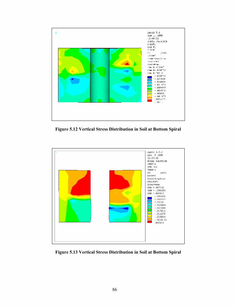
Figure 5.12 Vertical Stress Distribution in Soil at Bottom Spiral
Figure 5.13 Vertical Stress Distribution in Soil at Bottom Spiral
86

Figure 5.14 von Misses Stress Distribution in a Typical Spiral Plate –
View I
Figure 5.15 von Misses Stress Distribution in a Typical Spiral – View II
87

5.3.3 Installation Strength Analyses An installation failure FEA model was created to simulate a critical failure during
installation when the spiral encounters a hard rock, ice lens or other significant obstacle. The model used the same detail of the spiral structure as the Small Model but contained no soil elements. The spiral structure was restrained horizontally at an area of the outermost end of the bottom of the spiral and the bottom of the pipe was restrained against translation in the vertical direction as well as rotation about all but the vertical axis. A torque was applied at the top of the pipe section with a magnitude of 1,465 kN-m (90 kip-in), which is in the range used during installation of these piers (A. B. Chance, 1996). The spiral was modeled using the same material properties as in the Small Model with the addition of Bilinear Isotropic yield criteria (see Figure 5.3) including σy = 345 MPa (50 ksi) and ET = 10,000 MPa (1,450 ksi). This yield criterion allows for both elastic and plastic deformation of the elements. This model used shell elements with 4 nodes and 6 degrees of freedom at each node.
The helix and the center tube were modeled by shell elements. The special shape of the
helix made the FEA meshing very difficult. Several meshing techniques were used. The final FEA mesh shown in Figure 5.16 for the helix and central tube was carefully designed with most elements having good shapes and aspect rations which is significant important for accurate computational results.
Figure 5.17 shows a typical Installation Failure Model by FEA. The results from this
model show clearly that large stresses will develop at the weld between the spiral and the pipe. These stresses, reaching almost 500 MPa (72.5 ksi), are sufficient to yield the steel. This stress is highly concentrated at the bottom end of the connection and rapidly dissipates within an inch of this point.
The stress developed in the steel tube is much smaller than that in the helix. From the
stress contours in Figure 5.17 it is clear that the von Misses stress is highly concentrated at the connection near the leading edge. Stress level in this small area is several times higher than the average stress in the entire helix. These results are consistent with some, although rare, failure cases reported during installation procedure.
The developed FEA can be utilized in providing the accurate maximum stress under a
certain torque, or the maximum allowable torque without material failure. 5.3.4 Frozen Ground Creep Analyses
The Test Model was used in the development of a “creep model.” The material properties used were same as the previous models with the addition of creep parameters to simulate secondary creep effects over the period of two years. The computed design load of 22 kN (5 kip) was applied axially at the top of the pier.
88
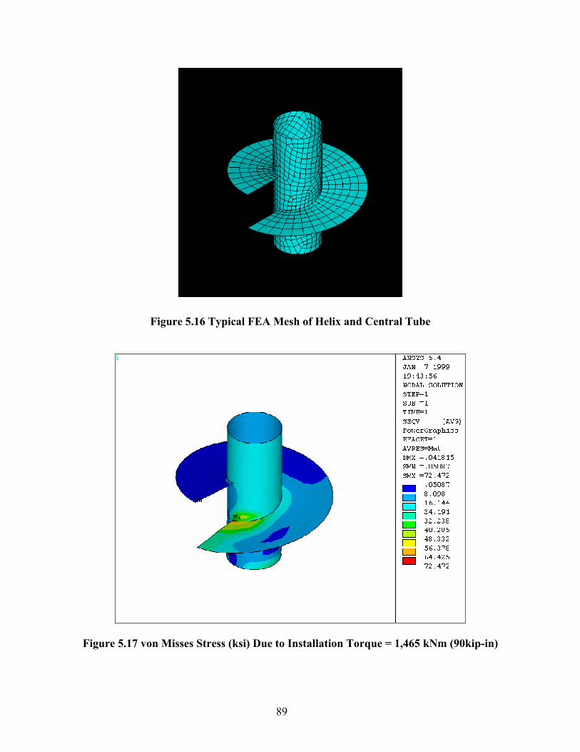
Figure 5.16 Typical FEA Mesh of Helix and Central Tube
Figure 5.17 von Misses Stress (ksi) Due to Installation Torque = 1,465 kNm (90kip-in)
89

The soil parameters used in this model are: friction angle, φ = 31°, c = 34 kPa (5 psi), unit weight = 20 kN/m3 (130 pcf), reference strain rate = 0.01 yr-1, creep modulus = 38 kPa (5.5psi), creep parameter n = 3.
According to original plan, the creep calculation results would compare with that from
the lab testing, therefore, creep calculations used the same dimension of soil model compatible with the lab setup. Figure 5.18 shows the creep displacement due to a constant axial load 22 kN (5 kip) for 2 years for Test Model.
The displacement results provided apply only to secondary settlement conditions and do
not account for primary or tertiary settlement. The initial settlement under the load was 30 mm (1.2 in) and increased to 40 mm (1.6 in), about 133% of the initial settlement over the course of two years. Some nonlinear displacement can be seen in Figure 5.18, indicating the possibility of boundary interaction between the base of the pier and the bottom of the soil volume. This effect should not been seen if Deep Model was used.
-4
-3.9
-3.8
-3.7
-3.6
-3.5
-3.4
-3.3
-3.2
-3.1
-30 100 200 300 400 500 600 700
Time (days)
Dis
plac
emen
t (cm
)
Figure 5.18 Creep Displacement Time History for a Shallow Model
The creep formula used in this study was based on equivalent von Misses stress due to surcharge on the soil. The FEA program will provide creep displacement due to total von Misses stress. Therefore, an approximation in the creep calculation is made on the correction for creep due to self-weight of the soil. Since the creep behavior of the system is nonlinear, it is mathematically incorrect to simply subtract the creep due to self-weight from the total creep. In addition, if self-weight of the soil were not used in the model, then the equivalent stress developed would not be accurate or reliable. Since the purpose of the research is to determine the
90

creep due to surcharge on the pier, it is necessary to account for the additional creep due to self-weight of the soil. However, creep analysis based on the weight of the soil only showed minimal displacement of the pier. Given that the displacement was so small, it was decided that the creep due to self-weight would be subtracted out as though it were a linear behavior. Since the research deals with the general behavior of a large area around the pier that is not dependent on extraneous accuracy, this approximation is appropriate for this analysis. It was recognized that this is not theoretically or mathematically correct, but there was no better way to do it. It seems to have no effect on the general results, though there are some anomalies in the data that may be related to this approximation.
Figure 5.19 shows the displacement time history for Deep Model with correction of self-
weight effects. The maximum net settlement of the Deep Model was 139 mm (5.49 in), which occurred under a 111 kN (25 kip) axial load, with the pier being displaced relatively rigidly. Figure 5.19 depicts the soil surface profile of Deep Model under various applied loads ranging from 0 kN to 111 kN. The initial displacement of the soil was due to the application of its self-weight only. The pier did not settle uniformly with the soil volume, consequently a bulge is evident at the surface of the soil. The gross displacement can be seen on the vertical axis and the net displacement, due to the applied load only, of the pier is indicated for each load step that was analyzed.
Distance
-30
-25
-20
-15
-10
-5
01 2 3 4 5 6 7 8 9 10 11 12 13
Dis
plac
emen
t (cm
)
0 kN
22.2 kN
44.4 kN
66.6kN
88.8kN
111 kN
Net Displacement = 0 cm
Net Displacement=1.78 cm, Design Load (FS=2)
Net Displacement= 4.45 cm,Ultimate Load (Eq 1)
Net Displacement= 7.24 cm
Net Displacement= 10.22 cm
Net Displacement= 13.94 cm
Displacement due to soil self weight
Figure 5.19 Surface Profile of the Deep Model Due to Various Loads
91

For piers with multiple helixes under small stress conditions, settlements due to applied loads will be almost the same as for corresponding single helix piers. However, under large stress conditions, the settlement is reduced with multiple helixes.
For the small stress condition, the stress results of two-helix pile indicated that the vertical compressive reaction stresses developed within the soil immediately after placement of the load were not distributed evenly between the plates. The stresses were concentrated at both the top and bottom plates, though the stress at the bottom plate was significantly higher. The reason for this may be attributed to the stiffness of the steel central column. The steel shaft is relatively very stiff between the two spiral plates, resulting in almost no shortening under the loading condition. The soil deformation between the two plates is mainly controlled by the steel deformation. Very small soil deformation would provide very small reaction stresses.
In addition to above sample analysis, a special model was created for the purpose of verifying the multi-helix effects of spiral plates. In this mode, four plates were connected to the central shaft. The results of this analysis indicated that the reaction stresses developed within the soil immediately after placement of the load were not distributed evenly among the plates. The reaction stresses directly below the bottom plate were several hundred percentages higher than in other regions. The fact that there was little significant contribution from the upper three spirals is likely to be caused by the confinement of the soil between the plates, which allows the soil in that volume to move for the most part, as a unit. To mobilize the soil strength the helixes need to be located at an adequate distance from each other. The study results show that a distance of three helix diameters between the helixes reduces creep under large stress.
The analysis results are consistent with the theoretical prediction. Based on Newtonian Mechanics for purposes of analyzing the statics or dynamics of a body, consider a force system whose force and moment resultants are identical. The force resultants, while equivalent, need not cause an identical distribution of strain, owing to a difference in the arrangement of the forces. In addition, Saint-Venant’s principle permits the use of an equivalent loading for the calculation of stress and strain. This principle states that, if an actual distribution of forces is replaced by a statically equivalent system, the distribution of stress and strain throughout the body is altered only near the regions of load application. Comparing single helix and multi-helix cases under the same load, the resultant reaction forces from the single helix and the multi-helix are the same. The stress and strain distributions are mainly identical in most of regions except near the helixes. The soil settlements are controlled by the soil deformation in most regions, not by the small region near the helixes. Therefore, the pile settlements are mainly the same in case of single-helix and multi-helix cases. However, stresses and strains in the area near the helixes are not the same in the cases of single and multi-helixes, which affects the stresses and strains within helixes.
For the large stress condition, due to the yielding of the soil under the bottom helix, the redistribution of stress is expected. When stresses in the soil under the bottom helix reach the yield level, the top helix would pick up more load. As a result, stresses are distributed more evenly between helixes and the average stress is smaller than that of the single helix condition. Therefore, the double helix will help to decrease the total creep settlement.
92

5.4 Summary of FEA
The findings from the development and the analysis of the FEA results are the following:
• The FEA model results will increase understanding of helical piers in various soil conditions as well as provide insight into design and installation considerations.
• The installation failure FEA model displayed the stresses encountered during installation of the pier system. The stress concentration that occurred at the bottom of the weld was very similar to known, but rare, failure mechanisms for helical piers. This information can be used to design better connection geometry at this critical location and emphasizes the need of good quality control during pier manufacturing.
• The FEA models provided valuable information regarding the distribution of stress and displacement within the soil. This stress may or may not depend on the geometry of the pier system in question. However, it does indicate that the soil reaction pressure is not equally distributed between two helices, and that the closely spaced spiral structures, even with three-helix-diameter spacing, will not provide significant increases in the overall capacity of the pier. As can be seen from the analysis of the two spirals spaced far enough apart in this pier system, only the bottom one contributes to any large extent to the pier’s capacity. Soil stress is not uniformly distributed under helixes as assumed by Equation (2.1). However, creep settlement under heavy loads and warm frozen temperatures is reduced by adding a second helix at least three helix diameters apart from the bottom helix.
• The detailed helix FEA models provided a close examination of the stresses within the spiral during the application of design loads. The highest stresses were encountered at the top and bottom ends of the spiral welds. This information can be used to make changes to the design of these structures if necessary as well as provide a more detailed picture of the physical situation encountered by helical structures embedded in soil.
• The creep FEA analysis indicated the creep behavior of helical piers in frozen ground and provides valuable insight into the magnitude of settlement that can be expected over extended periods of time. The creep deformation is not significantly different between piers with single or multiple helixes under small loads and cold under any load in cold frozen ground, but increases with the load and warming temperature.
• According to original plan, to validate the model, these results would have been compared with physical tests conducted at CRREL. The authors felt that the non-uniform test temperature and short loading time at the CRREL resulted in test results that could not be used to calibrate the FEA models.
5.5 References for Finite Element Modeling A. B. Chance Co., 1996, Helical Pier Foundation System Technical Manual, Bulletin 01-9601, Rev. 7/96, pp.2-7.
Das, B. M., 1998, Principles of Foundation Engineering, PWS Publishing, Fourth Edition.
93

Ghaly, A., Hanna, A., Ranjan, G. and Hanna, M., 1991, “Helical Anchors in Dry and Submerged Sand Subjected to Surcharge,” Journal of Geotechnical Engineering, Vol. 117, No. 10, pp. 1463-1470.
Johnston, G.H. and Ladanyi, B., 1974, “Field Tests of Deep Power-Installed Screw Anchors in Permafrost,” Canadian Geotechnical Journal, Vol. 11, No. 3, pp.348-358.
Ladanyi, B. and Johnston, G.H., 1974, “Behavior of Circular Footings and Plate Anchors Embedded in Permafrost,” Canadian Geotechnical Journal, Vol. 11, pp.531-553.
Ladanyi, B., 1983, “Shallow Foundations on Frozen Soil: Creep Settlement,” Journal of Geotechnical Engineering, Vol. 9, No. 11, pp.1434-1448.
Narasimha Rao, S. and Prasad, Y.V. N., 1993, “Estimation of Uplift Capacity of Helical Anchors in Clays”, Journal of Geotechnical Engineering, Vol. 119, No. 2, pp. 352-357.
Prasad, Y.V. N. and Narasimha Rao, S., 1996, “Lateral Capacity of Helical Piles in Clays,” Journal of Geotechnical Engineering, Vol. 122, No. 11, pp. 938-941.
94

6. DESIGN GUIDELINES 6.1 Development of Design Guidelines
The design guidelines are developed on the basis of the finite element analysis. For frozen ground, the dictating design criterion is the settlement due to the creep of the ice in the ground. The guidelines obtainable in the following sections are results from the Large Model (Deep Model) creep analysis. Input parameters for the analysis include material properties for the pier and the soil. The soil parameters include the strength parameters and creep parameters. These are functions of soil type, water content, unfrozen water content, and soil temperature. They vary greatly depending from location and season, and therefore, general guidelines cannot be provided for typical soil types, e.g. for sand, silt or clay. The following sections describe an example of design of helical piers for a silty soil at three different temperatures. To analyze any other soil, the engineer needs to contact the authors for FEA runs to produce the creep curves. 6.2 Materials and Model Dimensions: The soil properties for the silty soil are given in Table 6.1. The pier has a pipe shaft with 90 mm (3.5 in) outer diameter and 13 mm (0.5 in) thick wall, and a 203 mm (8 in) diameter, 13 mm (0.5 in) thick plate for a single spiral. For the large-scale model, the spiral is modeled as a flat plate in order to limit the number of elements in the model. The element and material properties for steel appear in Table 5.2. The soil surrounding the helical piers is modeled as a cylindrical volume. The dimensions used in the final analysis models are given in Table 6.2 and Figure 6.1.
Table 6.1. Soil Properties for Silty Soil
Unit Temperature
-1°C -5°C -10°C kN/m3 19.07 19.07 19.07 Unit Weight psf 119 119 119 kN/m2 2413 6206 9653 Cohesion psi 350 900 1400
Friction Angle ° 25 25 25 Creep Parameter, n 2.04 2.04 2.04
1/(h MPan)3.81*10-7 5.49*10-8 1.85*10-8 Creep Parameter, n
cuc
θσε 1&
1/(s ksin) 5.44*10-97.84*10-102.64*10-10
kPa 1800 7400 14400 Young's Modulus psf 37594 154553 300752 Poisson Ratio 0.2 0.2 0.2
95

Table 6.2 Dimensions of Final Calculation Models
H1
1
(mm) H2
(mm) H3
(mm) H
(mm) r
(mm) R
(mm) Single Helix Model 1270 - 2286 3556 203 1651 Double Helix Model 1270 610 2286 4166 203 1651
r
Soil Volume Soil Volume
Helical Piers
H2
H
r
H1 H1
H
H3
R R R R
H3
(a) Single Helix Model (b) Double Helix Model
Figure 6.1 Model Dimensions
6.3 Analysis Results The results of the FEA analysis are given in Table 6.3. Creep settlement (displacement) as a function of temperature is plotted in Figures 6.2 to 6.7. For the given soil, the creep displacement under various design loads is less than 3 mm (0.12 in) at temperatures from –1 to -10°C, which is less than a typical allowable settlement.
96
1 Pier manufacturers may recommend a larger minimum depth that could be conformed without affecting the creep curves significantly.
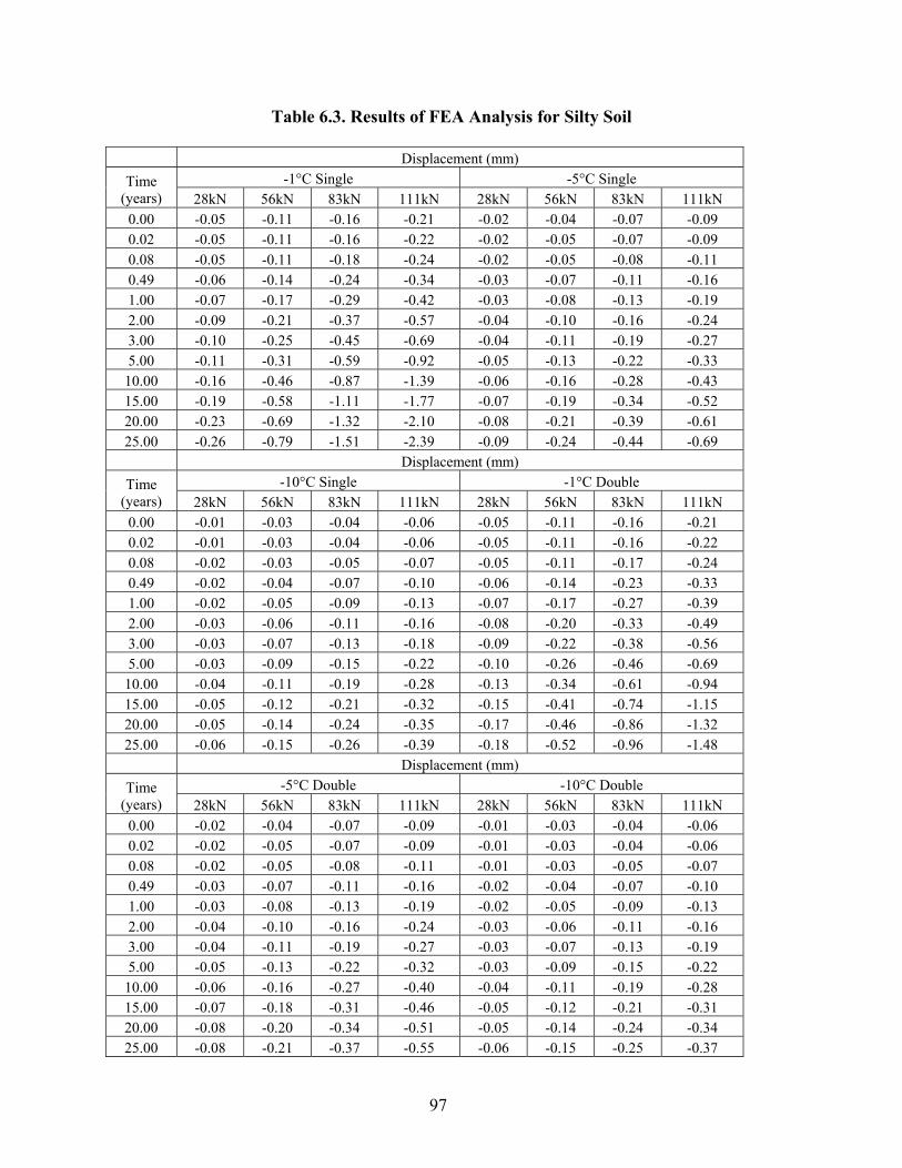
Table 6.3. Results of FEA Analysis for Silty Soil Displacement (mm)
-1°C Single -5°C Single Time (years) 28kN 56kN 83kN 111kN 28kN 56kN 83kN 111kN
0.00 -0.05 -0.11 -0.16 -0.21 -0.02 -0.04 -0.07 -0.09 0.02 -0.05 -0.11 -0.16 -0.22 -0.02 -0.05 -0.07 -0.09 0.08 -0.05 -0.11 -0.18 -0.24 -0.02 -0.05 -0.08 -0.11 0.49 -0.06 -0.14 -0.24 -0.34 -0.03 -0.07 -0.11 -0.16 1.00 -0.07 -0.17 -0.29 -0.42 -0.03 -0.08 -0.13 -0.19 2.00 -0.09 -0.21 -0.37 -0.57 -0.04 -0.10 -0.16 -0.24 3.00 -0.10 -0.25 -0.45 -0.69 -0.04 -0.11 -0.19 -0.27 5.00 -0.11 -0.31 -0.59 -0.92 -0.05 -0.13 -0.22 -0.33
10.00 -0.16 -0.46 -0.87 -1.39 -0.06 -0.16 -0.28 -0.43 15.00 -0.19 -0.58 -1.11 -1.77 -0.07 -0.19 -0.34 -0.52 20.00 -0.23 -0.69 -1.32 -2.10 -0.08 -0.21 -0.39 -0.61 25.00 -0.26 -0.79 -1.51 -2.39 -0.09 -0.24 -0.44 -0.69
Displacement (mm) -10°C Single -1°C Double Time
(years) 28kN 56kN 83kN 111kN 28kN 56kN 83kN 111kN 0.00 -0.01 -0.03 -0.04 -0.06 -0.05 -0.11 -0.16 -0.21 0.02 -0.01 -0.03 -0.04 -0.06 -0.05 -0.11 -0.16 -0.22 0.08 -0.02 -0.03 -0.05 -0.07 -0.05 -0.11 -0.17 -0.24 0.49 -0.02 -0.04 -0.07 -0.10 -0.06 -0.14 -0.23 -0.33 1.00 -0.02 -0.05 -0.09 -0.13 -0.07 -0.17 -0.27 -0.39 2.00 -0.03 -0.06 -0.11 -0.16 -0.08 -0.20 -0.33 -0.49 3.00 -0.03 -0.07 -0.13 -0.18 -0.09 -0.22 -0.38 -0.56 5.00 -0.03 -0.09 -0.15 -0.22 -0.10 -0.46 -0.69
10.00 -0.04 -0.11 -0.19 -0.28 -0.13 -0.34 -0.61 -0.94 15.00 -0.05 -0.12 -0.21 -0.32 -0.15 -0.41 -0.74 -1.15 20.00 -0.05 -0.14 -0.24 -0.35 -0.17 -0.46 -0.86 -1.32 25.00 -0.06 -0.15 -0.26 -0.39 -0.18 -0.52 -0.96 -1.48
Displacement (mm) -5°C Double -10°C Double Time
(years) 28kN 56kN 83kN 111kN 28kN 56kN 83kN 111kN 0.00 -0.02 -0.04 -0.07 -0.09 -0.01 -0.03 -0.04 -0.06 0.02 -0.02 -0.05 -0.07 -0.09 -0.01 -0.03 -0.04 -0.06 0.08 -0.02 -0.05 -0.08 -0.11 -0.01 -0.03 -0.05 -0.07 0.49 -0.03 -0.07 -0.11 -0.16 -0.02 -0.04 -0.07 -0.10 1.00 -0.03 -0.08 -0.13 -0.19 -0.02 -0.05 -0.09 -0.13 2.00 -0.04 -0.10 -0.16 -0.24 -0.03 -0.06 -0.11 -0.16 3.00 -0.04 -0.11 -0.19 -0.27 -0.03 -0.07 -0.13 -0.19 5.00 -0.05 -0.13 -0.22 -0.32 -0.03 -0.09 -0.15 -0.22
10.00 -0.06 -0.16 -0.27 -0.40 -0.04 -0.11 -0.19 -0.28 15.00 -0.07 -0.18 -0.31 -0.46 -0.05 -0.12 -0.21 -0.31 20.00 -0.08 -0.20 -0.34 -0.51 -0.05 -0.14 -0.24 -0.34 25.00 -0.08 -0.21 -0.37 -0.55 -0.06 -0.15 -0.25 -0.37
-0.26
97

Design Temperature -1°C Single
-3.00
-2.50
-2.00
-1.50
-1.00
-0.50
0.000.00 10.00 20.00 30.00
Time (years)
Dis
plac
emen
t (m
m)
28 kN56 kN83 kN111 kN
Figure 6.2. Creep Displacement for Single Helix Pier at Design Temperature of –1°C
Design Temperature -5°C Single
-0.70-0.60-0.50-0.40-0.30-0.20-0.100.00
0 10 20 30
Time (years)
Dis
plac
emen
t (m
m)
28 kN56 kN83 kN111 kN
Figure 6.3. Creep Displacement for Single Helix Pier at Design Temperature of –5°C
98

Design Temperature -10°C Single
-0.50
-0.40
-0.30
-0.20
-0.10
0.000 10 20 30
Time (years)
Dis
plac
emen
t (m
m)
28 kN56 kN83 kN111 kN
Figure 6.4. Creep Displacement for Single Helix Pier at Design Temperature of –10°C
Design Temperature -1°C Double
-1.60-1.40-1.20-1.00-0.80-0.60-0.40-0.200.00
0.00 10.00 20.00 30.00
Time (years)
Dis
plac
emen
t (m
m)
28 kN56 kN83 kN111 kN
Figure 6.5. Creep Displacement for Double Helix Pier at Design Temperature of –1°C
99

Design Temperature -5°C Double
-0.60
-0.50
-0.40
-0.30
-0.20
-0.10
0.000 10 20 30
Time (years)
Dis
plac
emen
t (m
m)
28 kN56 kN83 kN111 kN
Figure 6.6. Creep Displacement for Double Helix Pier at Design Temperature of –5°C
Design Temperature -10°C Double
-0.40-0.35-0.30-0.25-0.20-0.15-0.10-0.050.00
0.00 10.00 20.00 30.00
Time (years)
Dis
plac
emen
t (m
m) 28 kN
56 kN83 kN111 kN
Figure 6.7. Creep Displacement for Double Helix Pier at Design Temperature of –10°C
100
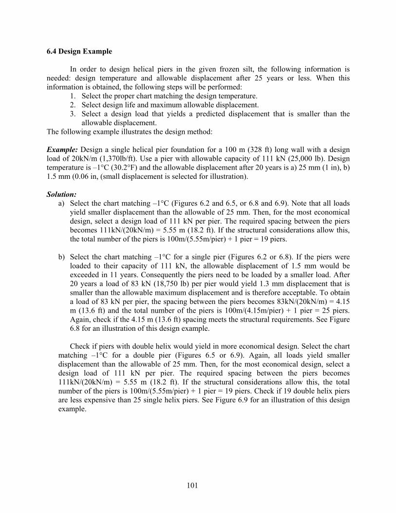
6.4 Design Example
In order to design helical piers in the given frozen silt, the following information is needed: design temperature and allowable displacement after 25 years or less. When this information is obtained, the following steps will be performed:
1. Select the proper chart matching the design temperature. 2. Select design life and maximum allowable displacement. 3. Select a design load that yields a predicted displacement that is smaller than the
allowable displacement. The following example illustrates the design method: Example: Design a single helical pier foundation for a 100 m (328 ft) long wall with a design load of 20kN/m (1,370lb/ft). Use a pier with allowable capacity of 111 kN (25,000 lb). Design temperature is –1°C (30.2°F) and the allowable displacement after 20 years is a) 25 mm (1 in), b) 1.5 mm (0.06 in, (small displacement is selected for illustration).
Solution:
a) Select the chart matching –1°C (Figures 6.2 and 6.5, or 6.8 and 6.9). Note that all loads yield smaller displacement than the allowable of 25 mm. Then, for the most economical design, select a design load of 111 kN per pier. The required spacing between the piers becomes 111kN/(20kN/m) = 5.55 m (18.2 ft). If the structural considerations allow this, the total number of the piers is 100m/(5.55m/pier) + 1 pier = 19 piers.
b) Select the chart matching –1°C for a single pier (Figures 6.2 or 6.8). If the piers were
loaded to their capacity of 111 kN, the allowable displacement of 1.5 mm would be exceeded in 11 years. Consequently the piers need to be loaded by a smaller load. After 20 years a load of 83 kN (18,750 lb) per pier would yield 1.3 mm displacement that is smaller than the allowable maximum displacement and is therefore acceptable. To obtain a load of 83 kN per pier, the spacing between the piers becomes 83kN/(20kN/m) = 4.15 m (13.6 ft) and the total number of the piers is 100m/(4.15m/pier) + 1 pier = 25 piers. Again, check if the 4.15 m (13.6 ft) spacing meets the structural requirements. See Figure 6.8 for an illustration of this design example.
Check if piers with double helix would yield in more economical design. Select the chart
matching –1°C for a double pier (Figures 6.5 or 6.9). Again, all loads yield smaller displacement than the allowable of 25 mm. Then, for the most economical design, select a design load of 111 kN per pier. The required spacing between the piers becomes 111kN/(20kN/m) = 5.55 m (18.2 ft). If the structural considerations allow this, the total number of the piers is 100m/(5.55m/pier) + 1 pier = 19 piers. Check if 19 double helix piers are less expensive than 25 single helix piers. See Figure 6.9 for an illustration of this design example.
101
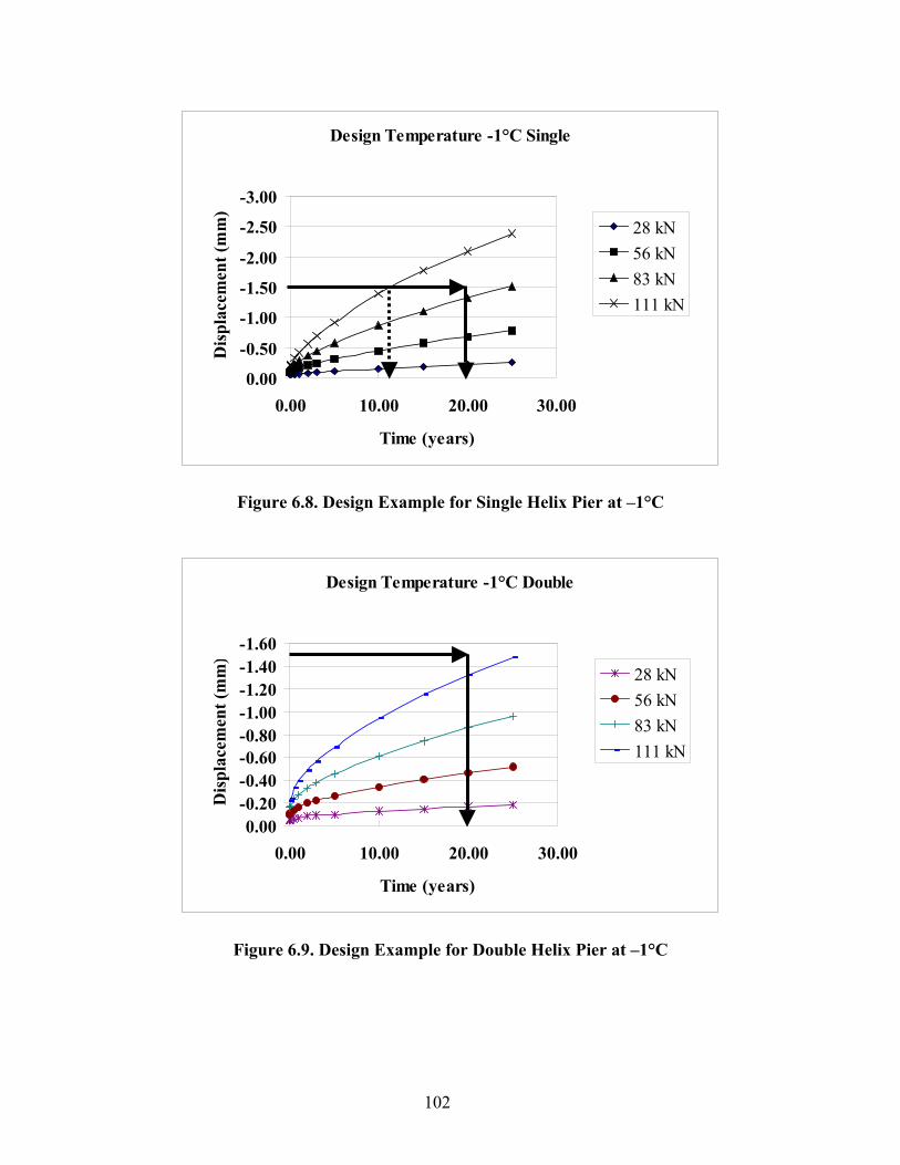
Design Temperature -1°C Single
-3.00
-2.50
-2.00
-1.50
-1.00
-0.50
0.000.00 10.00 20.00 30.00
Time (years)
Dis
plac
emen
t (m
m)
28 kN56 kN83 kN111 kN
Figure 6.8. Design Example for Single Helix Pier at –1°C
Design Temperature -1°C Double
-1.60-1.40-1.20-1.00-0.80-0.60-0.40-0.200.00
0.00 10.00 20.00 30.00
Time (years)
Dis
plac
emen
t (m
m)
28 kN56 kN83 kN111 kN
Figure 6.9. Design Example for Double Helix Pier at –1°C
102

6.5 Conclusions and Recommendations for Design
Even if specific design guidelines for frozen ground have not been in existence before, the piers are used successfully as a foundation for boardwalks and utilidors. However, engineers have been hesitating to specify helical piers as building foundations, because of the lack of design guidelines. The design method suggested here is very simple and helpful in designing piers for a given frozen soil. The design curves do not apply to any other soil than that given in Table 6.1, and even if the given creep displacements are insignificant, other soil properties may produce larger settlements. To properly design any foundations in frozen ground, the engineer still needs the creep parameters for the foundation soil. These parameters are not readily available for the engineering community. Therefore, actual soil testing needs to be conducted for various soils to create a library or database of soils encountered in cold regions. These tests would include strength parameters in thawed conditions, and creep and strength parameters at several frozen temperatures under various loads. Currently, to analyze any other soil, the engineer needs to contact the authors for FEA runs to produce the creep curves.
103

7. CONCLUSIONS AND RECOMMENDATIONS 7.1 Conclusions
The Evaluation of Helical Piers for Use in Frozen Ground project included a comprehensive literature review, field study, full-scale test at the CRREL, development of finite element models and creating design guidelines. The following findings were obtained during the work:
According to Literature Review, the design and performance of helical anchors and piers
in warm soils is analyzed using simple formulas that predict the field behavior adequately. However, the behavior of warm soils differs greatly from the behavior of frozen ground. The extent to which design principles for helical piers in warm soil applications are applicable to frozen ground is not currently understood. The behavior of piles in frozen ground is routinely estimated using adfreeze strength along the pile length. The design principles and mechanics for adfreeze piles cannot be directly applied to helical piers.
The findings from the full-scale test at CRREL indicated that the piers did not move at
-4°C under loads from 5.1 to 40.7 kN (1146 to 9140 lb). The results for the -1°C test indicated some movement, which was interpreted as a result of uneven temperatures on the soil basin and partial thaw settlement. The FEM could not be calibrated using the test results, because of the uneven temperatures in the test cell and the short loading times. Installation of the piers in the frozen ground proceeded without any problems.
The field study showed that the helical piers have been used by thousands in a variety of
projects in frozen ground in rural areas of Alaska. They have performed very well when installed below the active layer in cold, continuous permafrost. When firmly anchored in the permafrost they have resisted the forces of heaving and jacking. Results are also good in warm discontinuous permafrost, but there are more instances of heaving and jacking of the piers.
The developed FEA model results will increase understanding of helical piers in various
soil conditions as well as provide insight into design and installation considerations. The installation failure FEA model displayed the stresses encountered due to torque during installation of the pier system. The stress concentration that occurred at the bottom of the weld was very similar to known, but rare, failure mechanisms for helical piers. This information can be used to design better connection geometry at this critical location. The FEA models provided valuable information regarding the distribution of stress and displacement within the soil. According to the analysis, the soil stress is not uniformly distributed under helixes. Also, the analysis indicates that the soil reaction pressure is not equally distributed between the helixes. Only the bottom helix contributes to any large extent to the pier’s capacity.
The detailed helix FEA models provided a close examination of the stresses within the
spiral during the application of vertical design loads. The highest stresses were encountered at the top and bottom ends of the spiral welds. This information can be used to make changes to the design of these structures if necessary as well as provide a more detailed picture of the physical situation encountered by helical structures embedded in soil.
104

Finally, the creep FEA analysis indicated the creep behavior of helical piers in frozen
ground and provides valuable insight into the magnitude of settlement that can be expected over extended periods of time. The creep deformation is not significantly different between piers with single or multiple helixes.
According to original plan, to validate the FEA models, the results would have been
compared with physical tests conducted at CRREL. The authors felt that the non-uniform test temperature and short loading time at the CRREL resulted in test results that could not be used to calibrate the FEM.
The design method suggested includes simple design curves that are helpful in designing
piers for a given frozen soil. To analyze creep of helical piers in any other soil, the engineer needs to contact the authors for FEM runs to produce the creep curves.
7.2 Recommendations
Based on the literature review, field study, and the FEM results, it is concluded that the helical piers are suitable foundations for frozen ground. Their use is highly recommended for their ease of transportation and installation, small ground disturbance, resistance to pile jacking, and stability. It is recommended that foundation engineers and research and development engineers for pier manufacturers utilize the developed FEM.
7.3 Future Research Needs
The engineer has to contact the authors for design of a specific foundation in a given soil and design temperature. It would be more convenient if general design curves existed for a variety of soils at different design temperatures. Therefore, it is recommended that frozen soil properties would be determined for a multitude of typical foundation soils in Alaska and other cold regions.
Since the CRREL experiment could not be used to calibrate the FEM, additional tests are recommended for creep observations at controlled temperatures.
105

ACKNOWLEDGEMENTS
This research project was cooperation between the Alaska Science and Technology Foundation (ASTF), University of Alaska Anchorage (UAA), Alaska Foundation Technology, Inc (AFT) and U.S. Corps of Engineers Cold Regions Research and Engineering Laboratory (CRREL). The cash funding for the project was provided by the ASTF, while the UAA, AFT and CRREL provided in-kind contributions. The driving force behind the project was the AFT, a Chance® distributor, without whose persistence none of the work would have been possible. The authors, Dr. Zubeck and Dr. Liu would like to thank all participants for their financial support. They would also like to thank Tom Metlicka from AFT for his help throughout the project and for installing the piers at the CRREL, Dr. Vincent Janoo and Robert Eaton from CRREL for conducting and reporting the CRREL experiment, graduate student Lynn Aleshire for her remarkable contributions to the literature review and field study, students Sean Baginsky and Paul Kendal for their finite element analysis work and Todd Verdick for his help in the CRREL experiment. Gary Bowen was very helpful throughout the project in providing guidance and comments. Warm thanks also goes to Dan Schubert and Matt Dixon from the Alaska Native Tribal Health Consortium, Department of Environmental Health and Engineering, Roger Burleigh and Jon Menough from the State of Alaska Department of Environmental Conservation Village Safe Water for their tremendous help in the field study.
106
Copyright © 2022 FDOKUMEN