Evaluation of Approaches to Improve Longitudinal Joints in ...

Evaluation of Approaches to Improve Longitudinal Joints

in Mississippi Overlay Projects

Civil and Environmental Engineering Department

Department

Report Written and Performed By:

Ben C. Cox – Mississippi State University

Isaac L. Howard – Mississippi State University

Joe Ivy – Mississippi State University

Final Report

FHWA/MS-DOT-RD-15-250-Volume 3

December 2015

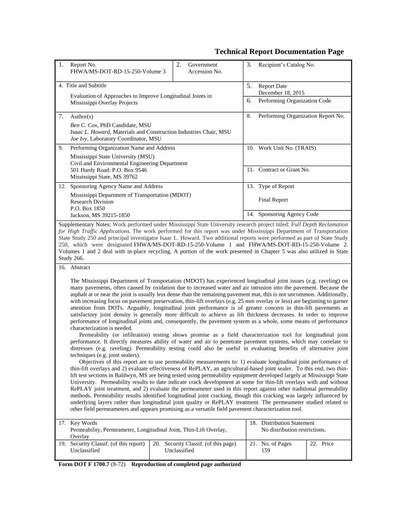
Technical Report Documentation Page

1. Report No.

FHWA/MS-DOT-RD-15-250-Volume 3

2. Government

Accession No.

3. Recipient’s Catalog No.

4. Title and Subtitle

Evaluation of Approaches to Improve Longitudinal Joints in

Mississippi Overlay Projects

5. Report Date

December 18, 2015

6. Performing Organization Code

7. Author(s)

Ben C. Cox, PhD Candidate, MSU

Isaac L. Howard, Materials and Construction Industries Chair, MSU

Joe Ivy, Laboratory Coordinator, MSU

8. Performing Organization Report No.

9. Performing Organization Name and Address

Mississippi State University (MSU)

Civil and Environmental Engineering Department

501 Hardy Road: P.O. Box 9546

Mississippi State, MS 39762

10. Work Unit No. (TRAIS)

11. Contract or Grant No.

12. Sponsoring Agency Name and Address

Mississippi Department of Transportation (MDOT)

Research Division

P.O. Box 1850

Jackson, MS 39215-1850

13. Type of Report

Final Report

14. Sponsoring Agency Code

Supplementary Notes: Work performed under Mississippi State University research project titled: Full Depth Reclamation

for High Traffic Applications. The work performed for this report was under Mississippi Department of Transportation

State Study 250 and principal investigator Isaac L. Howard. Two additional reports were performed as part of State Study

250, which were designated FHWA/MS-DOT-RD-15-250-Volume 1 and FHWA/MS-DOT-RD-15-250-Volume 2.

Volumes 1 and 2 deal with in-place recycling. A portion of the work presented in Chapter 5 was also utilized in State

Study 266.

16. Abstract

The Mississippi Department of Transportation (MDOT) has experienced longitudinal joint issues (e.g. raveling) on

many pavements, often caused by oxidation due to increased water and air intrusion into the pavement. Because the

asphalt at or near the joint is usually less dense than the remaining pavement mat, this is not uncommon. Additionally,

with increasing focus on pavement preservation, thin-lift overlays (e.g. 25 mm overlay or less) are beginning to garner

attention from DOTs. Arguably, longitudinal joint performance is of greater concern in thin-lift pavements as

satisfactory joint density is generally more difficult to achieve as lift thickness decreases. In order to improve

performance of longitudinal joints and, consequently, the pavement system as a whole, some means of performance

characterization is needed.

Permeability (or infiltration) testing shows promise as a field characterization tool for longitudinal joint

performance. It directly measures ability of water and air to penetrate pavement systems, which may correlate to

distresses (e.g. raveling). Permeability testing could also be useful in evaluating benefits of alternative joint

techniques (e.g. joint sealers).

Objectives of this report are to use permeability measurements to: 1) evaluate longitudinal joint performance of

thin-lift overlays and 2) evaluate effectiveness of RePLAY, an agricultural-based joint sealer. To this end, two thin-

lift test sections in Baldwyn, MS are being tested using permeability equipment developed largely at Mississippi State

University. Permeability results to date indicate crack development at some for thin-lift overlays with and without

RePLAY joint treatment, and 2) evaluate the permeameter used in this report against other traditional permeability

methods. Permeability results identified longitudinal joint cracking, though this cracking was largely influenced by

underlying layers rather than longitudinal joint quality or RePLAY treatment. The permeameter studied related to

other field permeameters and appears promising as a versatile field pavement characterization tool.

17. Key Words

Permeability, Permeameter, Longitudinal Joint, Thin-Lift Overlay,

Overlay

18. Distribution Statement

No distribution restrictions.

19. Security Classif. (of this report)

Unclassified

20. Security Classif. (of this page)

Unclassified

21. No. of Pages

159

22. Price

Form DOT F 1700.7 (8-72) Reproduction of completed page authorized

NOTICE

The contents of this report reflect the views of the author, who is responsible for the facts and

accuracy of the data presented herein. The contents do not necessarily reflect the views or

policies of the Mississippi Department of Transportation or the Federal Highway

Administration. This report does not constitute a standard, specification, or regulation.

This document is disseminated under the sponsorship of the Department of Transportation in

the interest of information exchange. The United States Government and the State of

Mississippi assume no liability for its contents or use thereof.

The United States Government and the State of Mississippi do not endorse products or

manufacturers. Trade or manufacturer’s names appear herein solely because they are

considered essential to the object of this report.

i

TABLE OF CONTENTS

LIST OF FIGURES ................................................................................................................. iii

LIST OF TABLES ................................................................................................................... iv

ACKNOWLEDGEMENTS .......................................................................................................v

LIST OF SYMBOLS ............................................................................................................... vi

CHAPTER 1 – INTRODUCTION ........................................................................................ 1

1.1 General and Background Information ...........................................................................1

2.1 Objectives and Scope .....................................................................................................1

CHAPTER 2 – LITERATURE REVIEW .............................................................................2

2.1 Overview of Literature Review .....................................................................................2

2.2 Permeability Concepts ...................................................................................................2

2.3 Permeability Measurement ............................................................................................5

2.4 Longitudinal Joint Permeability .....................................................................................7

2.5 Thin-Lift Pavements ......................................................................................................8

CHAPTER 3 – EXPERIMENTAL PROGRAM .......................................................10

3.1 Experimental Program Overview ................................................................................10

3.2 Test Equipment ............................................................................................................10

3.2.1 Permeameter Standpipe ...................................................................................10

3.2.2 MSP-F Water Supply .......................................................................................12

3.2.3 MSP-F Vehicle Support Frame ........................................................................13

3.2.4 MSP-LS and MSP-LL Test Frames ..................................................................13

3.3 Test Methods ................................................................................................................14

3.4 Thin-Lift Overlay Testing ............................................................................................15

3.5 MSP Comparison to Traditional Methods ...................................................................17

3.5.1 Part 1 ................................................................................................................17

3.5.2 Part 2 ................................................................................................................18

3.5.3 Part 3 ................................................................................................................20

ii

3.5.4 Part 4 ................................................................................................................20

CHAPTER 4 – THIN-LIFT OVERLAY PERMEABILITY RESULTS .........................21

4.1 Overview of Permeability Results ...............................................................................21

4.2 Longitudinal Joint Permeability ...................................................................................21

4.3 Pavement Mat Permeability .........................................................................................22

4.4 Permeability Ratio of Longitudinal Joint to Pavement Mat ........................................24

4.5 Thin-Lift Overlay Permeability Summary ...................................................................24

CHAPTER 5 – MSP EVALUATION RESULTS ...............................................................25

5.1 Overview of MSP Evaluation Results .........................................................................25

5.2 Test Results: Part 1 ......................................................................................................25

5.3 Test Results: Parts 2 to 4 ..............................................................................................26

5.4 MSP Evaluation Summary ...........................................................................................30

CHAPTER 6 – DISCUSSION, CONCLUSIONS, AND RECOMMENDATIONS .........32

6.1 Discussion ....................................................................................................................32

6.2 Conclusions ..................................................................................................................32

6.3 Recommendations ........................................................................................................33

CHAPTER 7 – REFERENCES ............................................................................................34

APPENDIX A – TEST SECTION PHOTOGRAPHS ....................................................... A1

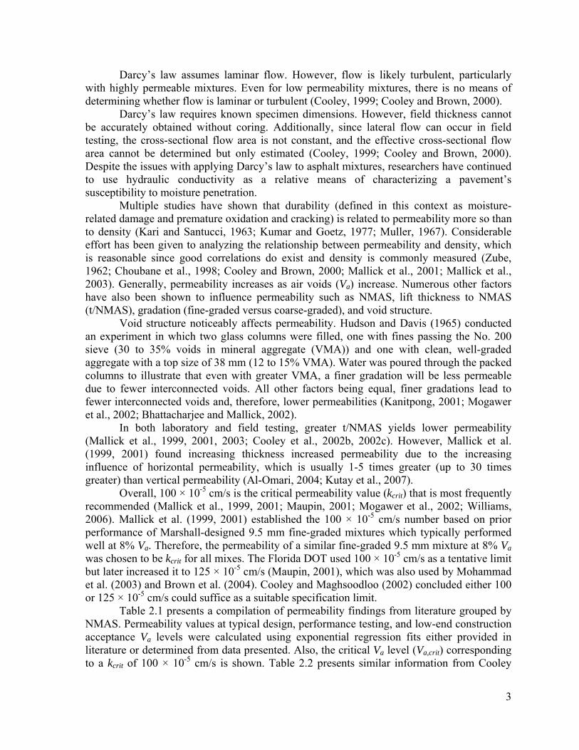
APPENDIX B – MSP-F PERMEAMETER DRAWINGS................................................ B1

APPENDIX C – MSP-LL PERMEAMETER DRAWINGS ............................................. C1

APPENDIX D – MSP-LS PERMEAMETER DRAWINGS .............................................. D1

iii

LIST OF FIGURES

Figure 2.1. Average Permeability vs. Air Voids by Nominal Maximum Aggregate Size ....5

Figure 2.2. Common Laboratory and Field Permeameters ....................................................5

Figure 2.3. Joint Permeability and Joint/Mat Permeability Ratio of Untreated and

Treated Longitudinal Joints (Mallick and Daniel, 2006; Williams

et al., 2009; Huang et al., 2010) ..........................................................................8

Figure 3.1. Permeameter Standpipe .....................................................................................12

Figure 3.2. MSP-F Water Supply Assembly .......................................................................12

Figure 3.3. Hitch-Mounted MSP-F Support Frame .............................................................13

Figure 3.4. MSP-L Equipment .............................................................................................14

Figure 3.5. MSP-F Field Permeability Testing ....................................................................15

Figure 3.6. Examples of Various Longitudinal Joint Qualities ...........................................16

Figure 3.7. Example Strip Test Layout for S1 .....................................................................18

Figure 3.8. Test Location Marking ......................................................................................18

Figure 3.9 TX and NCAT Permeameter Setups .................................................................19

Figure 3.10. MSP-LL Test Slabs Cut from Parking Lot.........................................................20

Figure 4.1. Permeability Results at Longitudinal Joint .......................................................21

Figure 4.2 Pavement Mat Permeability 0.3 m from Longitudinal Joint .............................23

Figure 4.3 Pavement Mat Permeability 0.6 m from Longitudinal Joint .............................23

Figure 4.4 Permeability Ratio of Longitudinal Joint and Pavement Mat ...........................24

Figure 5.1 Part 1 MSP-F Results by Strip and Location ....................................................26

Figure 5.2 Permeameter Relationships ...............................................................................28

Figure 5.3 Effects of Vacuum Saturation Time ..................................................................30

Figure 5.4 Comparisons of MSP-LS Conditioning Protocols on Inf ...................................30

iv

LIST OF TABLES

Table 2.1. Summary of Literature Permeability Values .......................................................4

Table 2.2. Summary of Mississippi Field Permeability from Cooley (2003) ......................4

Table 2.3. NCAT Volumetric Design Criteria for 4.75 mm NMAS Mixtures ....................9

Table 2.4. NCAT Gradation Limits for 4.75 mm NMAS Mixtures .....................................9

Table 3.1. List of Key Permeability Equipment Parts and Approximate Costs .................11

Table 3.2. Hwy 370 Test Location Summary Information .................................................16

Table 3.3. Hwy 371 Test Location Summary Information .................................................16

Table 3.4. Summary of Test Phases ...................................................................................17

Table 5.1 Part 1 MSP-F Inf Results ...................................................................................25

Table 5.2 Air Void and Thickness Data ............................................................................26

Table 5.3 Permeameter Comparison Results .....................................................................27

Table 5.4 MSP-LS Results by Conditioning Protocol .......................................................29

v

ACKNOWLEDGEMENTS

Thanks are due to many for the successful completion of this report. The MDOT Research

Division is owed special thanks for funding State Study 250. Mark Holley (District 1

Maintenance Engineer) and Joey Hood (District 1 Special Projects Officer) are owed thanks

for coordinating and assisting field data acquisition.

Dr. Thomas White of MSU is owed thanks for guidance related to development of the

permeameter used in this study. Several MSU students assisted with this effort by testing,

sorting data, producing equipment drawings, and similar. Chase Hopkins, Alyssa Leard, and

Braden Smith are owed special thanks for their efforts.

vi

LIST OF SYMBOLS

%Gmm Percent maximum mixture specific gravity

A Cross-sectional contact area

a Inside cross-sectional area of permeameter standpipe

AASHTO American Association of State Highway and Transportation Officials

APA Asphalt Pavement Analyzer

Avg Average

CF Empirical correction factor for TX permeameter

COV Coefficient of variation

D:B Ratio Dust to effective binder ratio

ESAL Equivalent Single Axle Load

FAA Fine aggregate angularity

FC Field compacted

h0,TX Starting water head for TX permeameter

h1 Initial head across the test specimen

h1,TX Water head measured at early test termination time for TX permeameter

h2 Final head across the test specimen

h2,TX Ending water head for TX permeameter

Inf Infiltration rate

IRI International Roughness Index

k Hydraulic conductivity

kcrit Critical hydraulic conductivity

L Test specimen thickness

L1 to L10 Parking lot locations 1 to 10

LC Laboratory compacted

MDOT Mississippi Department of Transportation

MSP Mississippi permeameter

MSP-F Mississippi permeameter – field configuration

MSP-LL Mississippi permeameter – laboratory configuration, large

MSP-LS Mississippi permeameter – laboratory configuration, small

NCAT National Center for Asphalt Technology

Ndes Design gyration level

Nini Initial gyration level

NMAS Nominal maximum aggregate size

PCR Pavement condition rating defined according to MDOT protocols

p-value Observed significance level

PVC Polyvinyl chloride

R2 Coefficient of determination

RAP Reclaimed asphalt pavement

S1 to S1 Parking lot strips 1 to 10

SE Sand equivalency

t Elapsed time between h1 and h2

tcorrected t2 corrected based on empirical testing for TX permeameter

t1 time of measurement for early test termination for TX permeameter

t2 expected flow time at end of test for TX permeameter

vii

t/NMAS Thickness to nominal maximum aggregate size

TSR Tensile strength ratio

Va Air voids

%Vbe,mix Effective binder volume expressed as percent of total mix

(i.e. VMA minus Va)

VMA Voids in mineral aggregate

V.S. Vacuum saturation

1

CHAPTER 1 – INTRODUCTION 1.1 General and Background Information

The Mississippi DOT (MDOT) has experienced longitudinal or centerline joint raveling on multiple pavements over the past several years. Longitudinal joint raveling is a problem faced by other state DOTs as well. It is often caused by aging (often via oxidation) due to increased water and air intrusion into the pavement as the asphalt at or near the joint is usually less dense than the rest of the asphalt in the roadway. With the increasing focus on pavement preservation, thin-lift overlays (e.g. 25 mm overlay or less) are garnering attention from DOTs. Arguably, longitudinal joint performance is perhaps of greater concern in thin-lift pavements as satisfactory joint density is likely more difficult to achieve relative to lifts of more conventional thickness. In order to improve longitudinal joint performance and, consequently, the pavement system as a whole, some means of characterization is needed.

A permeability or infiltration test appears to be one of the most suitable field measurements for characterizing longitudinal joint performance. It directly measures the ability of water to penetrate a pavement system, which has potential to be correlated to performance in categories of interest (e.g. raveling). Use of permeability tests could not only allow for better performance prediction but could also be useful in evaluating performance improvement of alternative longitudinal joint techniques (e.g. joint sealers). 1.2 Objectives and Scope The primary objective of this report is to use permeability measurements to: 1) evaluate the behavior of longitudinal joints of thin-lift overlays and 2) evaluate the effectiveness of RePLAY, an agricultural-based joint sealer. The objective was accomplished by conducting field permeability testing of two thin-lift test sections near Baldwyn, MS using permeability equipment developed largely at Mississippi State University (MSU). Ten test phases were conducted over a four year period. At each test phase, 27 locations were tested for a total of 270 tests overall. A secondary objective of this report is to compare the permeameter presented in this study to other traditional permeability methods. A total of 141 tests were conducted towards the secondary objective.

A literature review (Chapter 2) was conducted and used for guidance during analysis. The permeameters used as well as test methodology are provided in Chapter 3. Results from the permeability testing are presented in Chapters 4 and 5. Chapter 6 discusses project findings and provides concluding remarks and associated recommendations. Appendix A presents photographs of longitudinal joint test locations at each test phase. Appendices B, C, and D include complete technical drawings for permeameter equipment used herein.

This report was part of State Study 250, which was reported in three volumes. This report (Volume 3) focuses on thin-lift asphalt concrete joint permeability over time and is not directly related to Volumes 1 and 2. Volume 1 focuses on in-place recycling consisting of a wide variety of materials from asphalt concrete to fine grained soil (i.e. FDR). Volume 2 compliments Volume 1 in that it is also relates to in-place recycling, but addresses cold-in-place recycling (CIR). Some of the data presented herein related to the permeameter itself and was collected for dual purposes as it is useful to State Study 250 as well as a field aging study (State Study 266).

2

CHAPTER 2 – LITERATURE REVIEW

2.1 Overview of Literature Review

This report addresses three distinct topics: permeability, longitudinal joints, and thin-lift overlays. The structure of this literature review attempts to reflect the overall focus of the report in that discussion of each topic is provided herein. Sections 2.2 and 2.3 discuss permeability. Section 2.4 discusses longitudinal joints as they pertain to permeability. Section 2.5 discusses 4.75 mm nominal maximum aggregate size mixtures as thin-lift overlays are generally constructed with 4.75 mm mixtures. Additionally, a brief summary of current MDOT specifications for ultra thin asphalt mixtures is provided.

2.2 Permeability Concepts

Permeability is most commonly characterized by hydraulic conductivity (k) as described by Darcy’s law. Hydraulic conductivity is calculated by Eq. 2.1 for a falling head permeability test, which is the typical testing mode for asphalt mixtures. Appropriate use of Darcy’s law requires several assumptions to be valid; however, many of these assumptions are violated when testing asphalt mixtures, especially in the field.

2

1lnh

h

At

aLk (2.1)

Where, k = hydraulic conductivity (cm/s) a = inside cross-sectional area of permeameter standpipe (cm2) A = cross-sectional contact area (cm2) L = test specimen thickness (cm) t = elapsed time between h1 and h2 (s) h1 = initial head across the test specimen (cm) h2 = final head across the test specimen (cm)

Darcy’s law is only valid for one-dimensional flow. In field testing, water has the capability of flowing vertically or laterally (Cooley, 1999; Cooley and Brown, 2000). Tack coats between layers could also pose problems as they could prevent water from passing vertically through the entire layer and also contribute to forced lateral flow.

Darcy’s law assumes complete material saturation. At low degrees of saturation, apparent permeability is lower since water cannot flow through air bubbles according to Huang et al., 1999. However, Mallick et al. (1999, 2001) reported field permeability appeared to decrease with successive testing as pavements became increasingly saturated. It was suggested the pavement appears more permeable at first due to water filling voids, some of which are not interconnected. Therefore, the pavement takes in more water in the first few tests, giving an appearance of greater permeability. Regardless of whether saturation increases or decreases permeability, it does have a noticeable effect, yet degree of saturation cannot be accurately determined in the field (Cooley, 1999; Cooley and Brown, 2000).

3

Darcy’s law assumes laminar flow. However, flow is likely turbulent, particularly with highly permeable mixtures. Even for low permeability mixtures, there is no means of determining whether flow is laminar or turbulent (Cooley, 1999; Cooley and Brown, 2000).

Darcy’s law requires known specimen dimensions. However, field thickness cannot be accurately obtained without coring. Additionally, since lateral flow can occur in field testing, the cross-sectional flow area is not constant, and the effective cross-sectional flow area cannot be determined but only estimated (Cooley, 1999; Cooley and Brown, 2000). Despite the issues with applying Darcy’s law to asphalt mixtures, researchers have continued to use hydraulic conductivity as a relative means of characterizing a pavement’s susceptibility to moisture penetration.

Multiple studies have shown that durability (defined in this context as moisture-related damage and premature oxidation and cracking) is related to permeability more so than to density (Kari and Santucci, 1963; Kumar and Goetz, 1977; Muller, 1967). Considerable effort has been given to analyzing the relationship between permeability and density, which is reasonable since good correlations do exist and density is commonly measured (Zube, 1962; Choubane et al., 1998; Cooley and Brown, 2000; Mallick et al., 2001; Mallick et al., 2003). Generally, permeability increases as air voids (Va) increase. Numerous other factors have also been shown to influence permeability such as NMAS, lift thickness to NMAS (t/NMAS), gradation (fine-graded versus coarse-graded), and void structure.

Void structure noticeably affects permeability. Hudson and Davis (1965) conducted an experiment in which two glass columns were filled, one with fines passing the No. 200 sieve (30 to 35% voids in mineral aggregate (VMA)) and one with clean, well-graded aggregate with a top size of 38 mm (12 to 15% VMA). Water was poured through the packed columns to illustrate that even with greater VMA, a finer gradation will be less permeable due to fewer interconnected voids. All other factors being equal, finer gradations lead to fewer interconnected voids and, therefore, lower permeabilities (Kanitpong, 2001; Mogawer et al., 2002; Bhattacharjee and Mallick, 2002).

In both laboratory and field testing, greater t/NMAS yields lower permeability (Mallick et al., 1999, 2001, 2003; Cooley et al., 2002b, 2002c). However, Mallick et al. (1999, 2001) found increasing thickness increased permeability due to the increasing influence of horizontal permeability, which is usually 1-5 times greater (up to 30 times greater) than vertical permeability (Al-Omari, 2004; Kutay et al., 2007).

Overall, 100 × 10-5 cm/s is the critical permeability value (kcrit) that is most frequently recommended (Mallick et al., 1999, 2001; Maupin, 2001; Mogawer et al., 2002; Williams, 2006). Mallick et al. (1999, 2001) established the 100 × 10-5 cm/s number based on prior performance of Marshall-designed 9.5 mm fine-graded mixtures which typically performed well at 8% Va. Therefore, the permeability of a similar fine-graded 9.5 mm mixture at 8% Va was chosen to be kcrit for all mixes. The Florida DOT used 100 × 10-5 cm/s as a tentative limit but later increased it to 125 × 10-5 cm/s (Maupin, 2001), which was also used by Mohammad et al. (2003) and Brown et al. (2004). Cooley and Maghsoodloo (2002) concluded either 100 or 125 × 10-5 cm/s could suffice as a suitable specification limit.

Table 2.1 presents a compilation of permeability findings from literature grouped by NMAS. Permeability values at typical design, performance testing, and low-end construction acceptance Va levels were calculated using exponential regression fits either provided in literature or determined from data presented. Also, the critical Va level (Va,crit) corresponding to a kcrit of 100 × 10-5 cm/s is shown. Table 2.2 presents similar information from Cooley

4

(2003) for Mississippi pavements. Figures 2.1a and 2.1b plot the averaged permeability as a function of air voids for each NMAS. Generally, 9.5 mm and 12.5 mm mixtures have similar permeability characteristics relative to other NMAS mixtures (Cooley et al., 2002b, 2002c).

Table 2.1. Summary of Literature Permeability Values

LC/FCPermeameter Used R2

k (10-5 cm/s) at Va (%) Va,crit (%) NMAS Gradation Source 4 7 10

4.75 Fine West et al. (2011) FC PS129 --- 1 10 45 11.7 9.5 Both Mogawer et al. (2002) LC PS129 0.93 10 57 319 8.0

Fine Mogawer et al. (2002) FC NCAT 0.86 4 26 173 9.1 Coarse Mogawer et al. (2002) FC NCAT 0.75 1 15 201 9.2 Coarse Cooley et al. (2002b) FC NCAT 0.69 5 76 439 7.4 Coarse Cooley (2003) FC NCAT 0.75 1 69 840 7.4

Fine Cross and Bhusal (2009) FC NCAT 0.81 24 134 399 6.4 12.5 Both Mogawer et al. (2002) LC PS129 0.52 31 180 1043 6.0

Coarse Mogawer et al. (2002) FC NCAT 0.79 6 95 1602 7.1 --- Cooley et al. (2002b) FC NCAT 0.64 4 61 346 7.7

Both Cooley (2003) FC NCAT 0.53 2 41 317 8.2 19 Both Mogawer et al. (2002) LC PS129 0.16 15 33 74 11.1

Coarse Mogawer et al. (2002) FC NCAT 0.86 13 448 14876 5.7 --- Cooley et al. (2002b) FC NCAT 0.42 32 341 1534 5.2

Coarse Cooley (2003) FC NCAT 0.41 45 910 6190 4.6 25 Coarse Mogawer et al. (2002) FC NCAT 0.63 421 2126 10739 1.3 --- Cooley et al. (2002b) FC NCAT 0.50 126 1038 3987 3.8 -- LC/FC = laboratory-compacted/field-compacted. -- PS129 permeameter refers to the flexible-walled device developed in Florida and produced by Karol-Warner. -- NCAT permeameter refers to multi-tier type device developed by NCAT for use in the field. -- Va was determined by AASHTO T166. -- Va,crit corresponds to Va level at a permeability of 100 × 10-5 cm/s. Table 2.2. Summary of Mississippi Field Permeability from Cooley (2003)

Thickness (mm) R2

k (10-5 cm/s) at Va (%) Va,crit (%) NMAS Gradation 4 7 10

9.5 Coarse 35 0.53 9 90 397 7.2 Coarse 46 0.80 1 47 693 7.7

Coarse 44 0.87 11 200 1289 6.1 12.5 Coarse --- 0.79 3 54 376 7.8

Fine 51 0.67 0 12 124 9.7 Fine 48 0.52 1 193 6383 6.5 Fine 48 0.45 12 98 367 7.0

Fine 57 0.70 1 19 175 9.1 19 Coarse 58 0.35 92 572 1832 4.1

Coarse 49 0.76 6 292 3333 6.0 Coarse 70 0.48 122 2855 21279 3.9 Coarse 70 0.78 4 310 4806 6.0

Coarse 46 0.75 620 2709 6934 2.0 -- NCAT permeameter was used in all cases. -- Va was determined by AASHTO T166. -- Va,crit corresponds to Va level at a permeability of 100 × 10-5 cm/s.

5

a) All Mixtures in Literature b) Mississippi Mixtures

Figure 2.1. Average Permeability vs. Air Voids by Nominal Maximum Aggregate Size 2.3 Permeability Measurement

There are two types of falling head permeameters that are fairly prevalent: one laboratory device and one field device. The laboratory permeameter is a flexible-walled device used in Florida test method FM 5-565 and ASTM PS129 (now withdrawn) which is often referred to as the Karol-Warner device but is referred to herein as the PS129 device (Figure 2.2a). The field permeameter is a multi-tiered device developed by the National Center for Asphalt Technology (NCAT) which is referred to herein as the NCAT device (Figure 2.2b). Several variations of each device exist, but each maintains similar operating principles. Other permeameters have been evaluated as well. Some researchers have used air permeameters (James, 1998; Cross and Bhusal, 2009). Also, Wilson and Sebesta (2015) describe a simple permeameter following Texas specification Tex-246-F which is similar to the NCAT permeameter conceptually.

a) PS129 b) NCAT

Figure 2.2. Common Laboratory and Field Permeameters

0

50

100

150

200

250

300

350

400

0 2 4 6 8 10 12 14

Per

mea

bil

ity

(10-5

cm/s

)

Air Voids (%)

2.5 5.0 7.0 7.511.5

Va,crit (%)

2.5 5.0 7.0 7.511.5

Va,crit (%)

0

50

100

150

200

250

300

350

400

0 2 4 6 8 10 12 14

Per

mea

bil

ity

(10-5

cm/s

)

Air Voids (%)

12.5 mm9.5 mm

3.0 6.5 7.0

Va,crit (%)

6

Between the laboratory and field, laboratory permeability better satisfies Darcy’s law requirements as specimen dimensions are known, flow is one-dimensional, and specimens are pre-saturated. One-dimensional flow is achieved by confining pressure and a flexible membrane around the sides of a specimen. Vacuum saturation is conducted prior to testing to enhance repeatability, and testing is continued until results converge (crudely ensuring saturation is achieved). Permeability values are not significantly affected by test time interval or confining pressure (Hall et al., 2000). Additionally, sawing of specimens does not affect permeability as long as the saw blade is in good condition and consistent and reasonable contact pressure between the blade and specimen are used (Maupin, 2001).

Maupin (2001) observed considerable variability between operators as well as high variability between results (COV for field cores of 44% and COV for laboratory-compacted specimens of 0 to 133%). Therefore, with a small number of replicate specimens, approximately 50 × 10-5 cm/s or less must be targeted in order to reasonably ensure the actual permeability of the mixture is less than 100 × 10-5 cm/s. Bhattacharjee and Mallick (2002) found that porosity measured via vacuum sealing (ASTM D7063) correlated strongly to permeability and had approximately one-third the variability. While direct measurement would be the best indicator, porosity could be more reliable given the strong correlation and lower COV values.

While hydraulic conductivity, k, is usually calculated from field testing, field permeability measurements could be better characterized by infiltration rate (Eq. 2.2) as Darcy’s law does not apply in the field. Regardless, k is used as a relative measure of permeability. At low permeability, such as within the range agencies typically specify, field k is relatively comparable to laboratory k, but field measurements typically exceed laboratory measurements as permeability increases (Prowell and Dudley, 2002). This is due to the influence of horizontal permeability in the field since lateral flow is possible. Harris et al. (2011) showed that increasing permeameter contact area reduced permeability because the vertical cross-section (parallel to pavement surface) increased more so than the horizontal cross-section (parallel to pavement thickness), decreasing the effect of horizontal permeability on the final result. A permeameter with a 25 cm (10 in) diameter base (almost twice that of the standard NCAT permeameter) was recommended to minimize the effects of multi-dimensional flow.

)( 21 hhAt

aInf (2.2)

Where, Inf = infiltration rate (cm/min) a = inside cross-sectional area of permeameter standpipe (cm2) A = cross-sectional contact area (cm2) t = elapsed time between h1 and h2 (min) h1 = initial head across the test specimen (cm) h2 = final head across the test specimen (cm)

Saturation of in-place field pavements is difficult and impractical. Mallick et al.

(1999) neglected saturation effects completely and simply averaged three successive tests on a single test location to obtain a final result. It was argued that this method more realistically

7

simulated typical water infiltration of pavements (i.e. a pavement is likely unsaturated prior to a rain event). Harris et al. (2011) somewhat accounted for saturation effects by performing four successive tests and averaging the final three to obtain the permeability of a test location or test specimen. Permeability decreased with successive testing, especially between the first and second trials. The final three trials were not substantially different from each other (Harris et al., 2011).

The NCAT permeameter uses plumber’s putty or caulk to create a watertight seal to the pavement. This method is laborious and inhibits testing at previously-tested locations. Mallick et al. (1999, 2001, 2003) and Harris et al. (2011) used a neoprene foam rubber gasket and surcharge weight to provide the seal instead of putty or caulk. Mallick et al. (1999, 2001, 2003) used a series of ring-shaped weights totaling 47 kg (100 lb) as a surcharge.

The device built by Harris et al. (2011) was a two-tiered device based on the NCAT permeameter. It differed primarily in the sealing mechanism. The standpipe was connected to a steel box with a receiver ring on top. A PVC plate with a neoprene gasket attached and a hole of desired diameter (effect of permeameter size was of interest) was secured underneath the steel box. Vehicle self-weight was applied to box’s receiver ring via a hitch-mounted jack, which sealed the permeameter to the pavement.

Williams (2007) created 12.7 m2 (136 ft2) field permeability maps of seven pavements and found results can rely heavily on permeameter placement. Given the average variability of pavements, a minimum sample size of ten test locations per pavement was recommended. Cooley and Maghsoodloo (2002) conducted a round-robin study of the NCAT permeameter with seven operators. Each operator tested ten locations for each of eight pavements. They concluded the permeameter/operator reproducibility estimate (standard deviation) is 10 × 10-5 cm/s, and an overall standard deviation of permeability measurements is 24 × 10-5 cm/s. 2.4 Longitudinal Joint Permeability

Obtaining acceptable density levels at the longitudinal joint has been a longstanding concern in the context of long-term performance. In recent years, longitudinal joint permeability has been used as a means to gauge joint quality or to evaluate various joint construction techniques. Williams et al. (2009) found that permeability (reported as both hydraulic coefficient and infiltration rate) provided reasonable levels of discrimination (95% confidence) in terms of longitudinal joint quality, especially for those of lesser joint quality.

Mallick and Daniel (2006) built a three-standpipe permeameter that allowed simultaneous testing of longitudinal joints as well as the mat on either side of the joint. Untreated joint permeability ranged from approximately 2-50 times mat permeability. Williams et al. (2009) reported mat/joint permeabilities of approximately 4/8, 50/2,000, and 1,000/12,000 × 10-5 cm/s for three projects with good, fair to poor, and fair to poor joint quality ratings.

Mallick and Daniel (2006) studied various longitudinal joint construction techniques using the NCAT permeameter. Joint heaters decreased joint permeability relative to the control sections, but permeability was still 5-7 times that of the mat. Permeability of joints treated with sealers or adhesives was approximately equal to or even slightly less than that of the mat. Huang et al. (2010) evaluated the effects of various treatments on joint permeability (PS129 permeameter) in Tennessee. Four joint adhesives, two joint sealers, and an infrared

8

joint heater were evaluated. Relative to the untreated joint permeability of approximately 150 to 325 × 10-5 cm/s, three of the joint adhesives reduced permeability below 100 × 10-5 cm/s, and the infrared heater reduced permeability to approximately 40 × 10-5 cm/s. The joint sealers (one of which was RePLAY) had virtually no effect on joint permeability. It was hypothesized that the sealers could not withstand the high water head in PS129 but would fare better in terms of water penetration during a normal rainfall event; this was later confirmed by absorption tests in which the sealers performed well. Overall, joint sealers and adhesives appear promising.

Figure 2.3 provides longitudinal joint permeability values from Mallick and Daniel (2006), Williams et al. (2009), and Huang et al. (2010). The ratio of joint permeability to mat permeability is also provided. Figure 2.3 is intended to provide an overall understanding; therefore, each result shown is grouped into general categories by NMAS and treatment but not identified further. Relative to no treatment, joint treatments, specifically adhesives and sealers, appear relatively effective in reducing permeability to less than 100 × 10-5 cm/s. In general terms, 3 out of every 10 joints have a joint/mat permeability ratio of 10 or less, 4 out of every 10 have a ratio of 10-100, and 3 out of every 10 have a ratio of 100 or more.

Figure 2.3. Joint Permeability and Joint/Mat Permeability Ratio of Untreated

and Treated Longitudinal Joints (Mallick and Daniel, 2006; Williams et al., 2009; Huang et al., 2010)

2.5 Thin-Lift Pavements

Thin-lift overlays are typically less than 3.8 cm thick and can be used to address minor distresses, increase ride quality, and extend pavement life (Cooley et al., 2002a; Labi et al., 2005). Such states as Alabama, Maryland, Georgia, Michigan, New Jersey, and Ohio have used thin-lift overlays and 4.75 mm nominal maximum aggregate size (NMAS)

1

10

100

1,000

1

10

100

1,000

10,000

100,000

1 1 1 2 2 2 3 3 1 1 1 1 1 3 1 1 1 3 3 3 3 1 1 3 3

12.5 19 25 19 12.5 12.5

Untreated Joint Heater

Joint Adhesive Joint Sealer

Join

t/M

at P

erm

eab

ility

Rat

io

Join

t P

erm

eab

ility

(10

-5cm

/s)

Joint Permeability Joint/Mat Ratio12

.5NMAS

Reference

Treatment

9

mixtures with good success (West et al., 2011; Better Roads, 2011). Labi et al. (2005) performed an effectiveness analysis of thin-lift overlays in which International Roughness Index (IRI), rutting, and pavement condition rating (PCR) were evaluated. PCR was defined as a measure of surface distresses, such as transverse cracking, on a 0 to 100 scale, but a detailed description of the PCR calculation process was not provided. Depending on weather, traffic, and route type, approximate service life of thin-lift overlays is as follows when each performance indicator is used: 3-13 years (IRI), 3-14 years (rutting), and 3-24 years (PCR).

Cooley et al. (2002a) and West et al. (2011) established Superpave mix design criteria recommendations for 4.75 mm mixtures (Tables 2.3 and 2.4). Durability, as described by the authors of these works, was evaluated by tensile strength ratio and indirect tensile fracture energy. Stability was evaluated by APA rut depth. Suleiman (2011) tested several 4.75 mm mixtures and found that all met a 9.5 mm APA rut limit, likely due to the higher proportions of crushed fine aggregate to natural fine aggregate. Table 2.3. NCAT Volumetric Design Criteria for 4.75 mm NMAS Mixtures

Design ESAL Range (millions) Ndes

Min. FAA

Min. SE

Min. %Vbe,mix

Max. %Vbe,mix

%Gmm @ Nini

D:B Ratio

< 0.3 50 40 40 12.0 15.0 ≤ 91.5 1.0-2.0 0.3 to ≤ 3.0 75 45 40 11.5 13.5 ≤ 90.5 1.0-2.0 3.0 to ≤ 30 100 45 45 11.5 13.5 ≤ 89.0 1.0-2.0

-- Design Va Range = 4.0% to 6.0% -- Ndes = design gyration level -- D:B ratio = dust to binder ratio -- FAA = fine aggregate angularity -- SE = sand equivalency -- %Vbe,mix = effective binder volume (VMA minus Va) -- %Gmm @ Nini = percent maximum theoretical specific gravity at initial gyration level Table 2.4. NCAT Gradation Limits for 4.75 mm NMAS Mixtures

Sieve Size (mm)

% Passing Min. Max.

12.5 100 --- 9.5 95 100 4.75 90 100 1.18 30 55 0.075 6 13

Rahman et al. (2011a) detailed two 4.75 mm thin-lift overlay projects in Kansas. Lift

thicknesses were 19 mm and 16 mm. Some issues were experienced with placement during construction due to the thin nature of the overlay. Transverse cracks appeared to be the largest challenge in terms of performance, but smoothness and rutting did not appear to be of concern. Rahman et al. (2011b) concluded underlying pavement layers significantly influence performance of thin surface treatments.

MDOT Special Provision No. 907-411-1 dated June 28, 2010, outlines specifications for Mississippi’s ultra-thin asphalt pavements (UTAP). Thicknesses for a single lift are to be between 12.5 and 25 mm. A maximum of 30% natural sand and 25% reclaimed asphalt pavement (RAP) is allowed. Gradation requirements are as follows: 100% passing 12.5 mm, 95 to 100% passing 9.5 mm, ≥75% passing 4.75 mm, 22 to 70% passing 1.18 mm, and 4-12% passing 0.075 mm. A minimum FAA of 40 is required. Hydrated lime (1% by weight) is required. The design Va range is 4 to 6% at an Ndes of 50 gyrations. D:B ratio must be between 1.0 to 2.0, and %Vbe,mix must be greater than 12%. A minimum tensile strength ratio (TSR) of 0.85 is required. UTAP density is controlled by a “roll to refusal” pattern.

10

CHAPTER 3 – EXPERIMENTAL PROGRAM

3.1 Experimental Program Overview

An experimental program was developed to evaluate longitudinal joints of thin-lift overlays using permeability measurements. This program included evaluating benefits of a joint sealer to improve longitudinal joint performance. This program also included an evaluation of the permeameter used herein relative to traditional permeameters. This chapter discusses permeability test equipment (Section 3.2), permeability test methods (Section 3.3), thin-lift overlay testing (Section 3.4), and permeameter comparison testing (Section 3.5). 3.2 Test Equipment The equipment used in this research is similar to that used in the falling head permeability test developed by White (1975, 1976) and White and Ivy (2009). The original device was developed to evaluate open graded friction course (OGFC) mixtures and was adaptable for laboratory or field use. White and Ivy (2009) used the original device but with advancements made to the connections, mounting system, and water supply.

Further modifications were made by the authors of this report in order to create a testing equipment package which consists of a portable field testing system and two laboratory testing systems of varying size. One size is for larger test specimens such as slabs, while the other is for smaller test specimens such as field cores. Collectively, this system is referred to herein as the Mississippi permeameter (MSP) system. Individual permeameter configurations are denoted as follows: field permeameter (MSP-F), small laboratory permeameter (MSP-LS), and large laboratory permeameter (MSP-LL).

The MSP-LS and MSP-LL consist of a steel test frame and a permeameter standpipe. The MSP-F consists of a vehicle-mounted support frame, permeameter standpipe, and also a water supply. Table 3.1 provides a list of all major components required for the entire MSP system. These are discussed individually in subsequent sections. Complete shop drawings for all components are provided in Appendices B, C, and D.

Within the MSP testing system, the same permeameter standpipe is used in all three variations, which provides continuity between field and laboratory testing. The standpipe and some means of surcharge loading are the only critical components in terms of replicating the MSP concept. While the field water supply and test frames are convenient, there are other alternatives which could be used without comprising the test’s integrity. 3.2.1 Permeameter Standpipe The permeameter standpipe is shown in Figure 3.1 with individual parts listed in Table 3.1. The standpipe is machined from acrylic and has a 50.8 mm (2 in) inner diameter. Two grooves (illustrated in Figure 3.1a) are engraved into the standpipe marking 12.7 and 25.4 cm (5 and 10 in) of water head. These marks are used as reference points for the water height during testing. The base of the standpipe is 101.6 mm (4 in) diameter. There is a 6.3 mm (0.25 in) thick neoprene foam rubber gasket attached to the standpipe base via an adhesive backing. The neoprene foam rubber meets ASTM D1056 requirements and provides a watertight seal between the permeameter and pavement surface when the surcharge load is

11

applied. As shown in Figure 3.1a, quick-disconnect fittings allow for the attachment of braided tubing which carries water from a water supply to the permeameter. Table 3.1. List of Key Permeability Equipment Parts and Approximate Costs

ID Item Supplier Part No. Cost1 Permeameter Standpipe (Total Cost: $285 each) 1 Acryllic Standpipes, Aluminum Caps,

Fittings (each) Dillard Machine Service --- $225

2 12” × 24” Neoprene Foam Rubber Gasket (Durometer of 70A)

McMaster-Carr 8445K76 $60

MSP-F Water Supply (Total Cost: $820) 3 125 Gal. Water Tank w/ Bands ProTank 40298 & 61744 $280 4 Alta 12 VDC Remote Control Receiver

(50-100’ range) Bailey 301-206 $110

5 Jefferson 12 VDC 3/8” FNPT 2-Way Solenoid Valve

Fastenal 0490390 $115

6 Little Giant 12 VDC Utility Pump (80 gpm @ 40’ of water head)

Grainger 5UXN5 $85

7 Schumacher Electric 12 V, 1.5 A Trickle-Charge Battery Maintainer

McMaster-Carr 76025K11 $40

8 12 V Deep Cycle Battery & Box Automotive Store --- $110 9 Accessories (tubing, fittings, wiring, pallet) Hardware Store --- $80

MSP-F Support Frame (Total Cost: $2,030) 10 Fixed A-Frame Mount Top-Crank Jack

(2.5 ton lift capacity) McMaster-Carr 2933T11 $310

11 Gilson 250 lb. Load Ring (model 5502) Gilson HM-420 $520 12 Steel Support Frame & Extension Bars

(parts and labor) Dillard Machine Service --- $1,200

MSP-LS Small Test Frame (Total Cost: $910) 13 Fixed Through-Mount Top-Crank Jack


14 Gilson 250 lb. Load Ring (model 5502) Gilson HM-420 $520 15 Lower Base Plate (Steel Channel Section)

& Upper Base Plate (Steel Plate) --- --- $125

16 All Thread Steel Rod (3/4” × 36”) plus Hex Nuts and Flat Washers

--- --- $85

17 Polycarbonate Water Tray Assembly --- --- $60

MSP-LL Large Test Frame (Total Cost: $1,005) 18 Fixed Through-Mount Top-Crank Jack


19 Gilson 250 lb. Load Ring (model 5502) Gilson HM-420 $520 20 Lower & Upper Base Plate (Steel Plates) --- --- $220 21 All Thread Steel Rod (3/4” × 36”) plus Hex

Nuts and Flat Washers --- --- $85

17 Polycarbonate Water Tray Assembly --- --- $60

-- Additional details regarding equipment is located in Appendices B, C, and D 1) Estimated costs as of spring 2012

An aluminum cap is placed on top of the standpipe to distribute the surcharge load

from the test frame’s load ring to the standpipe. A button head screw is screwed into the bottom of the load ring (Figure 3.1b) to serve as a pivoting connection point between the load

12

ring and standpipe as shown in Figure 3.1c. This facilitates uniform sealing pressure between the standpipe and pavement.

Figure 3.1. Permeameter Standpipe

3.2.2 MSP-F Water Supply The MSP-F water supply assembly is shown in Figure 3.2 with individual parts listed in Table 3.1. A 473.2 liter (125 gallon) water tank and other control components are mounted to a plastic pallet for portability. When the water tank is drained, the entire assembly can be lifted into a truck bed by two people. Water flow is wirelessly controlled by a solenoid valve and pump via remote control. Power is supplied by a 12 Volt deep cycle battery which can be recharged by the onboard trickle charger.

a) Water Supply b) Water Supply Control Box

Figure 3.2. MSP-F Water Supply Assembly

ID 3

ID 9

Control Box (Fig. 3.2b)

ID 5

ID 4

ID 6

ID 7

ID 8

ID 1

ID 2

Grooves

Button Head Screw

Swivel connection between load ring and standpipe cap

a)

b)

c)

13

3.2.3 MSP-F Vehicle Support Frame The MSP-F vehicle support frame is shown in Figure 3.3 with individual parts listed in Table 3.1. A steel support frame is mounted into a vehicle’s receiver hitch. Extension bars (painted orange) can be attached during testing to facilitate testing over a wider area (e.g. a full lane width) but can be removed for travel, allowing the support frame to remain attached to the vehicle. A modified trailer jack mounts to the support frame rail and can travel the width of the entire frame for quick relocation of the permeameter in the transverse direction (i.e. perpendicular to direction of traffic). A load ring attached to the bottom of the jack is used to provide a consistent surcharge loading on the permeameter standpipe. Fabrication of the support frame was performed at a local machine shop. It should be noted that two diagonal braces were later added to the support frame to provide overall rigidity to the structure. These can be seen in Figure 3.3 but are not detailed in shop drawing appendices. Some aspects of the support frame, such as the diagonal braces, may be specific to the vehicle used and must be considered on a case by case basis.

Figure 3.3. Hitch-Mounted MSP-F Support Frame

3.2.4 MSP-LS and MSP-LL Test Frames The MSP-LS and MSP-LL laboratory test frames are shown in Figure 3.4. Both are similar in construction, consisting of an upper and lower steel base plate joined by four steel rods. Similar to the MSP-F, both laboratory frames are equipped with a jack and load ring to apply a surcharge load to the permeameter standpipe. The MSP-LS base dimensions are 30.5 cm by 30.5 cm, while the MSP-LL base dimensions are 50.8 cm by 50.8 cm. The MSP-LS test frame is designed for testing of pavement cores and is more portable than the MSP-LL. The MSP-LL is designed for testing larger specimens such as slabs, although cores can also be tested. In effect, the MSP-LL is more versatile (can test slabs or cores) but is more bulky and less portable than the MSP-LS.

In the laboratory, the MSP-F water supply is not needed. Instead, water is supplied using the same braided tubing which is connected to a water faucet. To contain runoff water during testing, water trays were built using polycarbonate sheets as shown in Figure 3.4c.

ID 10

ID 12

ID 11 Additional Braces

14

a) MSP-LL b) MSP-LS c) Water Tray

Figure 3.4. MSP-L Equipment 3.3 Test Methods

The falling head permeability test developed by White (1975, 1976) and recently used by White and Ivy (2009) was used for all testing performed herein. The upgraded MSP equipment discussed in the previous section was used herein. Test protocols are identical for all MSP permeameters. Once the permeameter standpipe is positioned over the test location, a 445 ± 22 N (100 ± 5 lb) surcharge load is placed on the permeameter by the load ring and jack assembly. Thereafter, the permeameter is filled with water to, or slightly above, the upper fill mark (25.4 cm of head). A timer is started when the water crosses the upper fill mark, and the time to fall a given distance is recorded. Figure 3.5 shows example photographs of testing with the MSP-F.

In this report, testing was generally terminated once the water reached the lower mark (12.7 cm of head) or after 5 minutes had elapsed, whichever came first. In some cases, testing continued beyond 5 minutes, but this was not common. If a test was terminated before water reached the lower mark, its fall distance was measured via a ruler taped to the standpipe.

Three successive replicates were performed one after another at each test location, and the results were averaged to form one test result. In nearly all cases, permeability decreased with each successive replicates; therefore, in cases where permeability was exceptionally low for the first replicate, the final two replicates were not conducted. Where pavements were impermeable, the final two replicates were not conducted either.

Infiltration rate, as calculated by Eq. 2.2, was used throughout this report as the preferred means of quantifying permeability. Infiltration rate was chosen over hydraulic conductivity (Darcy’s k) based on literature review. Additionally, for longitudinal joint testing, it was expected that cracks might develop at the joint over time. Under this expectation, the assumptions of Darcy’s law would be increasingly violated as horizontal flow through cracked channels within the pavement would increase. For these reasons, infiltration rate appeared to be a more suitable approach and was used for this research.

ID 18

ID 19

ID 21

ID 20

ID 13

ID 14

ID 16

ID 15 ID 17

15

Figure 3.5. MSP-F Permeability Testing

3.4 Thin-Lift Overlay Testing

Two thin-lift overlay test sections near Baldwyn, MS, were evaluated for this report and are denoted Hwy 370 and Hwy 371. Following construction, five and four test locations were selected from Hwy 370 and Hwy 371, respectively. A location was defined as a fixed longitudinal (i.e. with traffic direction) coordinate. A test site was defined as a fixed longitudinal and transverse (i.e. perpendicular to traffic direction) coordinate. Test sites were denoted A.B, where A represents the location number, and B denotes the transverse component (1 = over the center of the joint; 2 = 0.3 m (1 ft) laterally from the center of the joint; and 3 = 0.6 m (2 ft) laterally from the center of the joint). For example, at test location 1, sites tested were denoted 1.1, 1.2, and 1.3.

Selection of test locations was conducted to select locations of varying longitudinal joint quality. Longitudinal joint quality was visually evaluated and categorized as follows: good quality when the joint was not easily visible, moderate quality when the joint appeared to have the potential to open over time, and poor quality when the joint appeared to be somewhat open already. Figure 3.6 demonstrates examples of various joint qualities.

To allow each location to be re-tested with time, identifying markings were made during the first test phase as described in the remainder of this paragraph. An orange mark was made on one side of the pavement, the truck-mounted permeameter was placed at the centerline measurement location, and then a second orange mark was made that aligned the two marks with the permeameter for future coordinate re-location. GPS coordinates were also recorded to assist with re-alignment.

The longitudinal joint at some test locations was sealed with RePLAY Agricultural Oil Seal and Preservation Agent™. It is a biobased product that is marketed to penetrate pavements and retard oxidation and reduce moisture penetration. RePLAY was applied to select test locations of both Hwy 370 and Hwy 371 on July 11, 2011. A swath 0.6 m (2 ft) wide was sprayed centered over the longitudinal joint.

16

Figure 3.6. Examples of Various Longitudinal Joint Quality Definitions

At the Hwy 370 site, a nominal 19 mm UTAP overlay was placed in November 2010.

The total project length was 2.49 km (1.55 miles), and the eastbound lane was placed first. Table 3.2 summarizes Hwy 370 test locations. Test locations 1, 3, and 5 were sealed with RePLAY at an application rate of 0.131 L/m2 (0.029 gal/yd2). Testing at 0.3 and 0.6 m (1 and 2 ft) offsets from the longitudinal joint occurred in the eastbound lane only.

At the Hwy 371 site, a nominal 25 mm UTAP overlay was placed in November 2010. The total project length was 2.06 km (1.28 miles), and the northbound lane was placed first. Table 3.3 summarizes Hwy 371 test locations. Test locations 6, 7, and 9 were sealed with RePLAY at an application rate of 0.158 L/m2 (0.035 gal/yd2). Testing at 0.3 and 0.6 m (1 and 2 ft) offsets from the longitudinal joint occurred in the northbound lane only.

Table 3.2. Hwy 370 Test Location Summary Information ID GPS Coordinate Distance, m (ft)1 Joint Quality Landmark Sealed 1 N 34° 30’ 55.8” W 88° 37’ 27.0” 97.2 (319) Good Red & White House Yes 2 N 34° 30’ 55.9” W 88° 37’ 15.1” 278.0 (912) Moderate Beside Pasture No 3 N 34° 30’ 55.8” W 88° 37’ 02.3” 471.5 (1547) Moderate Between 2 Houses Yes 4 N 34° 30’ 56.0” W 88° 36’ 78.7” 830.6 (2725) Poor White House No 5 N 34° 30’ 56.1” W 88° 36’ 62.1” 1085.1 (3560) Poor Near Bridge Yes 1) Distance from beginning of new pavement on west end of project nearest Baldwyn. Table 3.3. Hwy 371 Test Location Summary Information ID GPS Coordinate Distance, m (ft)1 Joint Quality Landmark Sealed 6 N 34° 27’ 96.4” W 88° 28’ 91.6” 36.9 (121) Moderate Field Yes 7 N 34° 27’ 97.7” W 88° 28’ 90.8” 63.4 (208) Good Field Yes 8 N 34° 28’ 36.2” W 88° 28’ 77.7” 807.1 (2648) Poor Intersection No 9 N 34° 28’ 42.5” W 88° 28’ 77.8” 927.2 (3042) Poor White House Yes 1) Distance from new pavement nearest Prentiss and Itawamba county line. Field permeability testing was conducted in ten phases summarized in Table 3.4. Phase 1 testing was conducted prior to sealing with RePLAY. Phase 2 testing was conducted soon after RePLAY application. Thereafter, testing for the remaining eight phases occurred

ModerateGood Poor

JointJoint Joint

17

at nominal six month intervals, generally around June and December. In total, the field test sections were monitored for approximately four years. Table 3.4. Summary of Test Phases

Phase Test Times (months) Testing Date Temperature (°C) Nominal Actual Hwy 370 Hwy 371 Avg Min Max

1 Prior to sealing --- June 27, 2011 June 27, 2011 31.1 25.0 33.92 Immediately after sealing 0.5 July 26, 2011 July 26, 2011 30.7 25.0 35.6 3 6 months after sealing 5.1 Dec 13, 2011 Dec 14, 2011 12.0 5.6 17.8 4 12 months after sealing 10.2 May 16, 2012 May 15, 2012 25.3 18.9 28.9 5 18 months after sealing 17.8 Jan 3, 2013 Jan 4, 2013 5.1 -1.7 9.4 6 24 months after sealing 22.8 June 5, 2013 June 5, 2013 24.1 21.0 30.0 7 30 months after sealing 29.9 Jan 10, 2014 Jan 10, 2014 9.7 8.3 10.6 8 36 months after sealing 35.3 June 18, 2014 June 18, 2014 31.2 26.7 33.3 9 42 months after sealing 42.4 Jan 21, 2015 Jan 21, 2015 11.7 3.9 15.6 10 48 months after sealing 47.9 July 9, 2015 July 9, 2015 31.4 26.7 33.9

3.5 MSP Comparison to Traditional Methods A second test program was developed to compare the MSP system to other field and laboratory permeameters in use. Tests were conducted with all MSP configurations, the NCAT permeameter, the PS129 permeameter, and the Tex-246-F permeameter (further denoted the TX permeameter). Field and laboratory testing was conducted on a parking lot that was being monitored for a field aging study (MDOT State Study 266). Twelve strips of 12.5 mm NMAS asphalt mixture were paved where characteristics of each strip varied as described in Howard et al. (2012). Specific details are not provided in this report as they are not pertinent to the test program presented. Testing was laid out into four parts. 3.5.1 Part 1

In part 1, MSP-F testing was conducted on 6 of the 12 parking lot strips described in Howard et al. (2012). Strips 1, 3, 5, 7, 9, and 10 were tested, and ten locations were tested across each strip in a single transverse line. Test locations within a strip were spaced approximately 25 to 30 cm (10 to 12 in) apart depending on the width of the strip. Test locations were identified by strip and location (e.g. S1-L1 refers to Strip 1 and Location 1). In all, 60 locations were tested via MSP-F in phase 1, which took place over two days in June of 2015. Measured air temperature averaged 31.8 °C. Part 1 testing served to provide an assessment of MSP-F variability as well as locate nine test locations with a range of permeabilities for testing in parts 2 to 4.

Figure 3.7 shows Strip 1 as an example. A reference line was established where all test locations were marked with paint. Testing occurred 0.3 m (1 ft) away from this reference line in non-painted pavement areas. Test locations were marked with pavement chalk as shown in Figure 3.8 so that exact test locations could be relocated for subsequent testing. A plastic template with a 100 mm inner diameter and 150 mm outer diameter was used to mark a 150 mm diameter ring.

18

Figure 3.7. Example Strip Test Layout for S1

Figure 3.8. Test Location Marking

3.5.2 Part 2

In part 2, nine of the sixty test locations were selected based on MSP-F testing in phase 1. Three groups were identified where MSP-F results were lowest, highest, and approximately in the middle, in order to bracket results of all 60 locations. The nine locations selected were L7 to L9 for S1, S7, and S10. These nine locations were tested again in place with the NCAT and TX permeameters. Test intervals between MSP-F, NCAT, and TX permeability testing were spread out by 7 days or more so that the pavement’s moisture state could equalize between tests. TX permeability testing occurred in June of 2015; air temperature averaged 30.3 °C. Testing was conducted according to Tex-246-F and protocols described in Wilson and Sebesta (2015). The TX permeameter is shown in Figure 3.9a. It consists of a 150 mm diameter PVC pipe section with a manometer attached to the side. The wall thickness at the base is double that of the permeameter standpipe to provide a wider base for sealing to the pavement. The permeameter is sealed to the pavement with plumber’s putty similarly to the NCAT permeameter. Wilson and Sebesta (2015) reported flow time for water to fall from 36.8 to 11.4 cm (14.5 to 4.5 in) of water head. Tests were run a minimum of 5 minutes but were terminated prior to reaching 11.4 cm of head for longer tests. If terminated early, the early termination time (t1) and head (h1,TX) were recorded and forecasted to the expected flow time (t2) based on Equation 3.1. Equation 3.2 was used to empirically correct for overestimations of

Reference Line

S1-L10 S1-L5 S1-L1

Testing Line

0.3 m

Reference LinePlastic Template

Chalk Ring

0.3 m

19

Equation 3.1, reporting a corrected flow time (tcorrected) (Wilson and Sebesta, 2015). In this report, tests were conducted for 10 minutes, and tcorrected was calculated and used to obtain Inf according to Equation 2.2. Three test replicates were averaged and considered one test result.

Figure 3.9. TX and NCAT Permeameter Setups

TXTX

TXTX

hh

hhtt

,1,0

,2,012

ln

ln (3.1)

CF

tCFttcorrected

112 (3.2)

Where, t2 = expected flow time at end of test (min) (i.e. 11.4 cm water head) t1 = time of measurement for early test termination (min) h0,TX = starting water head (36.8 cm) h1,TX = water head measured at early test termination time (cm) h2,TX = ending water head (11.4 cm) tcorrected = t2 corrected based on empirical testing (min) CF = empirical correction factor (0.2) NCAT permeability testing occurred in June of 2015; air temperature averaged 29.5 °C. Approximately 0.6 kg (1.25 lbs) of plumber’s putty was used to create a 7.5 cm (3 in) seal around the outside circumference of the permeameter base approximately 12.5 mm thick. The permeameter was placed over the test location and firmly seated for a watertight seal. To maintain the seal during testing, four 2.3 kg weights were placed on the permeameter base as shown in Figure 3.9b. Tests were conducted for five minutes per replicate; three replicates were averaged for one test result. Darcy’s k was calculated by Equation 2.1. Specimen thickness for Equation 2.1 was obtained later on cores cut from test locations.

a) TX b) NCAT

20

3.5.3 Part 3 In part 3, nine slabs were cut from parking lot test locations first tested by MSP-F, NCAT, and TX permeameters in part 2, and subsequently tested in the laboratory using the MSP-LL permeameter. Slabs (Figure 3.10) were cut using a walk-behind wet saw, transported to the laboratory, and fan-dried approximately 3 weeks. MSP-LL testing was conducted according to the test method described in Section 3.3.

Figure 3.10. MSP-LL Test Slabs Cut from Parking Lot

3.5.4 Part 4 In part 4, 150 mm diameter cores were cut from the center of slabs tested in part 3 and were tested using the MSP-LS and PS129 permeameters (note that the MSP-LL could have been used in place of the MSP-LS). Cores were fan-dried approximately 3 weeks between coring and initial testing. MSP-LS testing was conducted according to Section 3.3. PS129 testing was conducted according to ASTM PS129.

Multiple specimen conditions were considered in part 4 MSP-LS testing. Specimens were initially tested after fan drying. Specimens were also tested after 1, 3, and 5 minutes of vacuum saturation at 575 mm Hg based on PS129. Lastly, 5-minute vacuum saturated specimens with petroleum jelly sealed sides were tested. This last condition was evaluated in attempts to reduce the ability of water to flow out of specimen sides; however, it was not intended to force one-dimensional flow through the specimen as in PS129 (water exits the bottom of the specimen).

With field permeability testing, water, at least to some extent, has the ability to flow horizontally through the pavement and resurface some distance away from the permeameter. Likewise, with the sealed MSP-LS testing, water was able to flow in a similar manner since the permeameter base (100 mm diameter) is smaller than the core (150 mm diameter). This experiment was conducted to reduce edge effects expected when testing cores rather than slabs or essentially infinite field pavements and not to replicate PS129 flow patterns.

PS129 testing was conducted according to ASTM PS129 (Darcy’s k reported) with the exception that cores were not sliced on the bottom to remove tack coat layers. Rather, core bottom texture was relatively open and resulted in numerous flow paths. Cores were dried in the CoreDry® device in between each test conducted.

Note void structure may have been clogged by sawing slurry

21

CHAPTER 4 – THIN-LIFT OVERLAY PERMEABILITY RESULTS

4.1 Overview of Permeability Results

This chapter presents Hwy 370 and Hwy 371 permeability results, characterized in this chapter by infiltration (Inf). Data acquired from tests prior to sealing (Phase 1) through four years of service (Phase 10) is presented. Each result is generally the average of three replicate tests as stated in Section 3.3. 4.2 Longitudinal Joint Permeability Figure 4.1 provides all longitudinal joint Inf results. Recall that each test location is categorized by whether or not it is sealed as well as subjective joint quality. Generally, Inf decreased within the first several months; this is likely due to surface void closure as a combined result of high temperatures, traffic, and high asphalt content. Locations sealed with RePLAY were not meaningfully differentiated from those not sealed.

a) Hwy 370

b) Hwy 371

Figure 4.1. Permeability Results at Longitudinal Joint

0.4 8.

9

9.3

50.2

49.8

0.2 3.1

1.0

2.3

22.3

0.1

0.4

0.6

1.6

0.7

0.2

1.2

0.3

1.4

0.6

0.3

1.6

0.3

0.8

0.5

0.1 2.9

0.2

0.3

0.6

0.0

13.1

0.1

0.8

0.2

0.1

62.4

0.2

0.2

0.3

0.1

108.

9

0.1

0.3

0.4

0.1

20.3

0.1

0.2

0.1

0

20

40

60

80

100

120

Y N Y N Y

Good Moderate Moderate Poor Poor

1 2 3 4 5

Inf(

cm/m

in)

Prior to Sealing Imm. After Sealing6 mo. 12 mo.18 mo. 24 mo.30 mo. 36 mo.42 mo. 48 mo.

Sealed (Y/N)

Test Location

Joint Quality

11.2

28.5

11.7

65.2

5.1

3.7

1.6

3.4

1.5

2.8

1.9

2.1

4.1

2.5

1.3

20.6

41.6

1.6

0.8

71.8

11.5

1.1 4.2

27.9

16.8

0.6

2.6

135.

5

9.7

2.1

40.9

95.3

13.3 20

.2

99.8

127.

0

9.4

3.1

95.3

99.8

0

20

40

60

80

100

120

140

160

Y Y N Y

Moderate Good Poor Poor

6 7 8 9

Inf(

cm/m

in)


Sealed (Y/N)

Test Location

Joint Quality

22

Inf at locations 2, 8, and 9 increased over time, which corresponded to physical observations of longitudinal joint cracking. Location 6 Inf suggests opening of the longitudinal joint to a lesser degree. Longitudinal joint cracking was physically observed at Location 6 as can be seen in Appendix A photographs. Hereafter, locations 2, 6, 8, and 9 are referred to as cracked locations. For cracked locations, Inf was generally lower during summer test phases than winter test phases, which is not beyond reason. Cracks usually close up during warmer temperatures when the pavement expands and open in colder temperatures when the pavement contracts. Regarding subjective joint quality ratings assigned to each test location, both locations rated good (and both sealed with RePLAY) exhibited low Inf over time, though results suggest a crack may have begun forming at location 7 towards the end of the 4-year monitoring period. Three locations were rated moderate; location 2 exhibited high Inf over time, location 6 exhibited moderate Inf over time, and location 3 exhibited insignificant Inf. Of these, location 2, which exhibited the highest Inf, was not sealed with RePLAY. When only considering locations rated good and moderate, RePLAY appears that it could have had some positive effects on Inf performance. Four locations were rated poor. Locations 4 and 5 exhibited insignificant Inf while locations 8 and 9 Inf was considerably high. In this case, one location in each Inf group was sealed with RePLAY and one was not. For poor-rated locations, Inf results appear less dependent on RePLAY treatment. Reflective longitudinal joint cracking from underlying pavement layers appears to drive Inf more so than thin-lift overlay joint quality or treatment. At cracked locations, thin-lift overlay longitudinal joints were centered on underlying layer longitudinal joints; therefore, reflective joint cracking showed up in MSP-F testing. For other locations, either underlying layer joint cracking was not present, or at least had not reflected to the surface, or the longitudinal joints of underlying layers and the thin-lift overlay were not aligned so that reflected joint cracking was not detected by MSP-F testing. Location 5 is an example of a case where underlying layer and thin-lift overlay joints were not aligned; Appendix A photographs show reflected cracking several centimeters from the thin-lift overlay joint. Overall, permeability results suggest longitudinal joint performance of the thin-lift overlays tested is not necessarily a great concern as long as the longitudinal joint of underlying layers is in relatively good condition. It is less apparent as to whether RePLAY was beneficial for joint permeability and overall performance. For example, location 4 was not sealed, was of poor quality, and nonetheless yielded Inf comparable to other non-cracked locations that were sealed. Where reflective cracking occurred at the thin-lift overlay joint, Inf appeared sufficiently informative in detecting these cases. 4.3 Pavement Mat Permeability Figure 4.2 and 4.3 provide Inf results for test sites which were 0.3 m and 0.6 m laterally from the longitudinal joint, respectively. As with Figure 4.1, Inf initially decreased at early test times, also likely due to surface void closure. Inf values for the pavement mat are considerably lower than at the joint and remain low throughout the entire 4-year monitoring period. Most locations were essentially impermeable after the first 12 months of service. Note that a crack formed at location 8 (Figure 4.2) at 42 months (winter) but was closed up during 48 month testing (summer).

23

a) Hwy 370

b) Hwy 371

Figure 4.2. Pavement Mat Permeability 0.3 m from Longitudinal Joint

a) Hwy 370

b) Hwy 371

Figure 4.3. Pavement Mat Permeability 0.6 m from Longitudinal Joint

1.8

1.8

0.8

0.3

1.3

0.7

0.3

0.3

0.2

0.10.2

0.2

0.1

0.1

0.00.

3

0.1

0.1

0.0

0.00.

2 0.3

0.1

0.0 0.

1

0.1

0.1

0.1

0.0 0.1

0.0

0.0

0.0

0.0

0.0

0.0

0.0

0.0

0.0

0.0

0.0

0.0

0.0

0.0

0.0

0.0

0.0

0.0

0.0 0.1

0.0

0.5

1.0

1.5

2.0

1 2 3 4 5

Inf(

cm/m

in)


Test Location

0.0

1.1

0.2

0.0

0.0 0.1 0.3

0.0

0.0

0.0 0.1

0.0

0.0

0.0

0.1

0.0

0.0

0.0

0.0

0.0

0.0

0.0

0.0

0.0

0.0

0.0

0.1

0.0

0.0

0.0

0.0

0.0

0.0

0.0

3.7

0.0

0.0

0.0

0.0

0.0

0

1

2

3

4

6 7 8 9

Inf(

cm/m

in)


Test Location

0.1

1.3

1.6

0.7

0.4

0.1

1.0

0.4

0.1

0.0

0.0 0.

1 0.2

0.0 0.

1

0.0 0.

1

0.1

0.0

0.0

0.0

0.3

0.2

0.0 0.1

0.0 0.1

0.1

0.0

0.0

0.0

0.0 0.1

0.0

0.0

0.0

0.0

0.0

0.0

0.0

0.0

0.0

0.0

0.0

0.0

0.0

0.0

0.0

0.0

0.0

0.0

0.5

1.0

1.5

2.0

1 2 3 4 5

Inf(

cm/m

in)


Test Location

0.3 0.

4

0.0 0.

2

0.1 0.

3

0.1

0.00.

2

0.2

0.0

0.0

0.0 0.

1

0.0

0.00.1

0.1

0.0

0.0

0.0

0.0

0.0

0.0

0.0

0.0

0.0

0.0

0.0

0.0

0.0

0.0

0.0

0.0

0.0

0.0

0.0

0.0

0.0

0.0

0.0

0.5

1.0

1.5

2.0

6 7 8 9

Inf(

cm/m

in)


Test Location

24

4.4 Permeability Ratio of Longitudinal Joint and Pavement Mat Figure 4.4 provides the ratio of longitudinal joint permeability to pavement mat permeability (0.3 m and 0.6 m offsets averaged). For impermeable locations, joint-to-mat Inf ratio was not applicable. In general, the Inf ratio was 1 to 10 for 4 out of every 10 cases, 10 to 100 for 4 of 10 cases, and greater than 100 in 15% of cases. This trend could be partly explained by two factors. First, mat permeabilities were relatively low, which is reasonable for a small NMAS asphalt mixture (see Figure 2.1a for supporting data from literature). Second, ratios increased over time as Inf increased for cracked locations. Overall, this distribution is skewed more towards lower Inf ratios than those presented in Section 2.4.

a) Hwy 370

b) Hwy 371

Figure 4.4. Permeability Ratio of Longitudinal Joint and Pavement Mat 4.5 Thin-Lift Overlay Permeability Summary Findings from MSP-F permeability testing indicated that thin-lift overlay longitudinal joint performance is more influenced by underlying layers and less influenced by joint quality or RePLAY treatment. Increasing Inf values for cracked locations corresponded well with crack development which was physically observed. Pavement mat permeability was considerably lower than at the joint, resulting in joint-to-mat Inf ratios which were relatively close to but slightly less than joint-to-mat ratios documented in literature.

0.4

5.7

7.9

97.4

58.5

0.5

4.8

2.9 15

.2

337.

4

1.5

2.2

3.9

48.6

8.9

1.3

9.5

3.5

3.1

5.3

1.8

4.7

1.3

45.6

3.0 17

.3

2.0

3.2 10

.7

4.0

3930

.7

20.0

7.0

2556

.8

4.9 10

.3

3.7

0.1

1.0

10.0

100.0

1000.0

10000.0

Y N Y N Y

Good Moderate Moderate Poor Poor

1 2 3 4 5

Join

t/M

at I

nf

Rat

io


Sealed (Y/N)

Test LocationJoint Quality

n/a

n/a

n/a

n/a

n/a

n/a

n/a

n/a

n/a

n/a

n/a

n/a

n/a

88.1

37.5 12

3.0 81

4.5

153.

4

19.2

8.218

.5

29.1

36.4

42.1

40.0

1309

.9

50.7

82.5

133.

8

53.2

1257

1.4

0.1

1.0

10.0

100.0

1000.0

10000.0

100000.0

Y Y N Y

Moderate Good Poor Poor

6 7 8 9

Join

t/M

at I

nf

Rat

io

Prior to Sealing Imm. After Sealing 6 mo.12 mo. 18 mo. 24 mo.30 mo. 36 mo. 42 mo.48 mo.

Sealed (Y/N)

Test Location

Joint Quality

n/a

n/a

n/a

n/a

n/a

n/a

n/a

n/a

n/a

n/a

n/a

n/a

n/a

n/a

n/a

n/a

n/a

n/a

n/a

n/a

n/a

n/a

n < 1: 4% 1 < n < 10: 44% 10 < n < 100: 37% n > 100: 15%

25

CHAPTER 5 – MSP EVALUATION RESULTS

5.1 Overview of MSP Evaluation Results

This chapter evaluates the MSP permeameter system in the context of traditional permeability methods. Section 5.2 discusses part 1 results and MSP-F variability. Section 5.3 discusses comparisons of part 1 to part 4 results. 5.2 Test Results: Part 1 Table 5.1 presents Inf results from MSP-F testing for all 60 parking lot test locations (6 strips, 10 locations per strip). Values are also plotted in Figure 5.1 for visual assessment. In several cases, Inf is much greater for locations near the edge of a strip, such as L1 or L10. Higher permeability is characteristic of lower density pavement sections; typically, edges of a pavement mat, especially the unsupported or free edge, exhibit lower density. Therefore, results with and without the outer L1 and L10 locations were considered. Table 5.1. Part 1 MSP-F Inf Results

Inf (cm/min) by Strip and Location

1 3 5 7 9 10

L1 2.39 0.62 0.24 0.06 3.41 7.09 L2 1.41 0.46 0.77 0.16 2.38 3.63 L3 1.05 0.42 0.26 0.59 0.83 2.46 L4 1.08 0.47 0.22 0.74 0.23 2.36 L5 0.78 0.41 0.65 0.28 0.44 1.52 L6 1.05 1.17 0.84 0.52 0.47 0.93 L7 1.08 0.59 1.96 0.49 0.69 5.30 L8 0.90 3.88 0.41 0.53 0.46 6.42

L9 1.02 1.51 0.33 0.79 0.90 6.19 L10 4.63 9.23 0.49 0.34 2.67 5.61

AvgAll 1.54 1.88 0.62 0.45 1.25 4.15 COVAll (%) 77 149 84 53 91 54

Avg8 1.05 1.11 0.68 0.51 0.80 3.60 COV8 (%) 17 107 83 42 85 59

With the exception of Strips 5 and 7, the average Inf when all 10 locations were considered (AvgAll) was higher than when only the inner 8 locations were considered (Avg8). In general, coefficient of variability (COV) was higher for all 10 locations (COVAll) than for the middle 8 (COV8). Except for Strip 1, COV8 is considerably large for most strips, which is generally a result of one extreme permeability value remaining in each strip after outer locations were removed (i.e. S3-L8, S5-L7, S9-L2). Although variability is high, this is somewhat to be expected based on findings of Williams (2007), which recommended ten test locations at a minimum to provide a representative average. For further testing in parts 2 through 4, nine locations of the sixty were selected. S7 and S10 exhibited the lowest and highest average Inf, respectively, with S1 providing mid-range Inf. For each strip, locations 7, 8, and 9 were selected for consistency between strips.

26

Figure 5.1. Part 1 MSP-F Results by Strip and Location

5.3 Test Results: Parts 2 to 4 This section presents results from parts 2 through 4 and compares them with part 1 results. First, Table 5.2 presents air void (Va) and thickness (L) data for the nine cores obtained from the nine selected test locations in part 1. Note that air voids and thicknesses were not measured until part 4; however, their values were used in part 2 calculations. Second, comparisons between MSP-F, MSP-LL, MSP-LS, NCAT, TX, and PS129 permeameters are presented. Third, effects of various specimen conditioning and preparation procedures for the MSP-LS are presented. Table 5.2 presents Va (AASHTO T331 measured) and thickness data. Since some internal water was anticipated to be present in the nine cored specimens, core Va’s were adjusted using previously-collected data from other parking lot cores not studied in this report. At the time that core bulk gravities were determined, it was estimated that approximately 0.7% of each core’s mass was water, which was subtracted from each core’s mass to obtain dry masses (i.e. no internal moisture). Relative to the cores not fully dried, this adjustment increased Va approximately 0.7% on average. Table 5.2 Va’s are moisture-adjusted. On average, S9 Va was slightly lower than S1 Va, which was considerably lower than S10 Va; these air voids support MSP-F Inf trends in Section 5.2. Table 5.2. Air Void and Thickness Data

S1 S7 S10 Va (%) L (mm) Va (%) L (mm) Va (%) L (mm)

L7 8.8 75.0 8.4 77.0 9.5 73.1 L8 8.8 72.0 9.4 75.1 11.2 70.6 L9 10.3 70.2 9.5 73.1 12.0 65.5 Avg 9.3 72.4 9.1 75.1 10.9 69.7 COV (%) 9 3 7 3 11 6

Table 5.3 presents permeability results for all permeameters following standard test methods. Inf was reported for MSP-F, MSP-LL, MSP-LS, and TX permeameters, while Darcy’s k was reported for NCAT and PS129 permeameters. Table 5.3 MSP-F data is

0

1

2

3

4

5

6

7

8

9

10

1 3 5 7 9 10

Inf(

cm/m

in)

Strip

L1 L2 L3 L4 L5

L6 L7 L8 L9 L10

27

identical to corresponding Table 5.1 and 5.3 data is the same and is shown in Table 5.3 for convenience. Table 5.3. Permeameter Comparison Results

Core ID MSP-F Inf (cm/min)

MSP-LL Inf (cm/min)

MSP-LS Inf (cm/min)

TX Inf (cm/min)

NCAT k (10-5 cm/sec)

PS129 k (10-5 cm/sec)

S1-L7 1.08 1.47 1.34 0.66 46.2 12.4 S1-L8 0.90 0.84 0.89 2.54 127.2 10.5 S1-L9 1.02 1.47 1.25 2.96 162.3 26.3 S7-L7 0.49 0.57 1.08 0.67 69.3 4.2 S7-L8 0.53 1.62 2.71 0.65 67.8 6.6 S7-L9 0.79 0.83 2.02 0.88 117.0 8.2 S10-L7 5.30 1.14 3.60 2.14 312.2 10.5 S10-L8 6.42 1.61 4.25 6.33 441.8 74.9 S10-L9 6.19 1.12 4.28 4.82 385.6 285.8

Figure 5.2 plots relationships comparing MSP-F with other permeameters, including the two laboratory MSP configurations. Figure 5.2a shows that MSP-LL and MSP-F were similar for S1 and S7; however, MSP-LL S10 Inf values were less than 20% of MSP-F values. Review of data did not reveal any noticeable errors. Ultimately, the authors have no explanation for the MSP-LL S10 results, but given the dramatic differences between them and MSP-F S10 results, they are cause for attention. Figure 5.2a suggests there are potentially other variables at play that are not considered herein such as fines produced when cutting slabs that may have clogged void structures or temperature differences between field and laboratory testing. At present, the authors do not fully understand Figure 5.2a. Figure 5.2b shows that MSP-LS to MSP-F relationships are more reasonable than for MSP-LL, although MSP-LS S10 Inf values were still slightly lower than for MSP-F. For S1 and S7, MSP-LS yielded slightly higher Inf values than MSP-F and MSP-LL. This trend is not unreasonable since MSP-LS tests were conducted on cores (MSP-LL conducted on slabs); therefore, horizontal water flow paths to a boundary were shorter, and more water was likely to exit core sides, increasing Inf. Overall, R2, at 0.81, is satisfactory. Figure 5.2c shows that TX and MSP-F permeameters yielded similar Inf on average with moderate correlation (R2 is 0.66), though a moderate amount of scatter was present for any one result. Figure 5.2d shows a good relationship between NCAT and MSP-F results (R2 of 0.94). For both TX and NCAT permeameters, standpipe inner diameter is considerably larger than for MSP, approximately 15 cm versus 5 cm. This is potentially meaningful given the relatively rough surface texture present in some parking lot areas tested.

Howard et al. (2012) documented check cracking after compaction for the parking lot test section; permeability testing occurred after approximately 3.5 years of aging, which could have further promoted surface crack formation. For the NCAT and TX permeameters, their larger diameters imply the circumference of the base is resting on different cracks than for the MSP-F device. However, both the NCAT and MSP-F have relatively wide seals in comparison to the TX permeameter. Wider seals would be more likely to better seal surface cracks and decrease surface texture’s influence on permeability results. Narrower seals, like that of the TX, would be less likely to completely span surface cracks, allowing water to more easily flow under the seal rather than through the pavement. The TX’s narrower seal could have contributed to the greater observed variability than with the NCAT device.

28

Figure 5.2e shows that a modest relationship exists between PS129 and MSP-F permeameters (R2 is 0.43). However, significant spread of data is observed for S10. Figure 5.2e emphasizes one of the major differences between PS129 and all other permeameters studied. PS129 forces all water to pass completely through the core; whereas, horizontal flow and seepage just below the surface along surface cracks is possible with other permeameters. Figure 5.2f shows the NCAT to PS129 relationship yielded a similar trend in which there was considerable scatter and NCAT k values were considerably higher.

a) MSP-LL vs. MSP-F b) MSP-LS vs. MSP-F

c) TX vs. MSP-F d) NCAT vs. MSP-F

e) PS129 vs. MSP-F f) NCAT vs. PS129

Figure 5.2. Permeameter Relationships

y = 0.04x + 1.09R² = 0.06

0

1

2

3

4

5

6

7

0 1 2 3 4 5 6 7

MSP

-LL

Inf

(cm

/min

)

MSP-F Inf (cm/min)

S1S7S10Equality

y = 0.47x + 1.18R² = 0.81

0

1

2

3

4

5

6

7

0 1 2 3 4 5 6 7

MSP

-LS

Inf

(cm

/min

)MSP-F Inf (cm/min)

S1S7S10Equality

y = 0.63x + 0.81R² = 0.66

0

1

2

3

4

5

6

7

0 1 2 3 4 5 6 7

TX

Inf

(cm

/min

)

MSP-F Inf (cm/min)

S1S7S10Equality

y = 55.20x + 52.85R² = 0.94

0

100

200

300

400

500

0 1 2 3 4 5 6 7

NC

AT

k(1

0-5cm

/sec

)

MSP-F Inf (cm/min)

S1S7S10

y = 23.10x - 9.48R² = 0.43

0

50

100

150

200

250

300

0 1 2 3 4 5 6 7

PS1

29 k

(10-5

cm/s

ec)

MSP-F Inf (cm/min)

S1S7S10

y = 1.04x + 141.15R² = 0.41

0

100

200

300

400

500

0 100 200 300 400 500

NC

AT

k(1

0-5cm

/sec

)

PS129 k (10-5 cm/sec)

S1S7S10Equality

29

Overall, the greatest differences between permeameters were observed with S10 data. In some cases, such as with PS129, these differences seem intuitive, but in others, such as with MSP-LL and MSP-LS, these differences seem less intuitive. S10 data aside, MSP-F and MSP-L relationships appear reasonable. Further investigation comparing MSP-F and MSP-L permeameters seems necessary to make reliable statements regarding their relationships. Laboratory to field relationship establishment was not successful in the limited study performed.

Reasonable correlations were obtained between MSP-F and TX or NCAT permeameters, while weaker correlation was obtained between MSP-F and PS129 permeameters. This finding supports general expectations given the fundamental characteristics of each permeameter. Figure 5.2 is useful in providing a reference for between-permeameter relationships (e.g. excluding the y-intercept offset, NCAT k is approximately 55 times MSP-F Inf for the units reported). Based on Figure 5.2d, the recommended 100 × 10-5 cm/sec permeability threshold for the NCAT permeameter is equivalent to 0.85 cm/min MSP-F Inf. Table 5.4 presents results when conditioning protocols (e.g. vacuum saturation (V.S.)) were considered. All Table 5.4 results are for the MSP-LS permeameter. MSP-LS results with no conditioning (identical to those in Table 5.3) are presented for reference. Table 5.4. MSP-LS Results by Conditioning Protocol

MSP-LS Inf (cm/min) by Conditioning Protocol Saturation (%) by AASHTO T283

Core ID None V.S. (1 min)

V.S. (3 min)

V.S. (5 min)

V.S. (5 min) & Sealed

V.S. (1 min)

V.S. (3 min)

V.S. (5 min)

V.S. (5 min) & Sealed

S1-L7 1.34 1.14 2.02 1.85 0.92 49 45 46 35 S1-L8 0.89 0.95 0.85 0.93 0.89 50 57 52 45 S1-L9 1.25 1.57 1.21 1.67 0.79 60 65 61 56 S7-L7 1.08 1.03 0.79 1.18 0.75 47 46 50 44 S7-L8 2.71 2.53 2.68 2.57 1.87 49 54 55 46 S7-L9 2.02 1.93 1.55 1.99 1.96 46 54 52 47 S10-L7 3.60 4.88 2.33 3.34 2.91 52 59 57 49 S10-L8 4.25 4.10 3.79 4.16 4.14 53 55 57 53 S10-L9 4.28 5.93 6.15 4.85 5.45 51 53 56 49 -- V.S. = vacuum saturation according to PS129 with varying vacuum times -- Sealed denotes core sides were sealed with petroleum jelly Figure 5.3 demonstrates the relationship between vacuum saturation time and core saturation (%) using Table 5.4 data. There is no relationship. Therefore, further evaluation considered only two groups: 1) vacuum saturated, and 2) vacuum saturated and sealed with petroleum jelly. Figure 5.4a presents an equality plot comparing vacuum-saturated Inf results to Inf results with no conditioning (i.e. relatively dry specimens). All vacuum saturation times are considered simultaneously since saturation was independent of vacuum time. Overall, there was little difference between saturated and unconditioned results. Figure 5.4b compares vacuum saturated and sealed Inf results to Inf results for unconditioned cores. Relative to Figure 5.4a, the trendline shifts downward slightly, indicating vacuum saturated and sealed specimens exhibit slightly lower permeability than vacuum saturated or unconditioned cores. This trend is reasonable since sealed sides would

30

force more water through the core rather than allowing it to flow out of the side. However, the relationship is not greatly different, which may be due to water’s ability to flow under the permeameter base and resurface elsewhere on the top of the core as discussed in Chapter 3.

Figure 5.3. Effects of Vacuum Saturation Time

a) MSP-LS Inf after V.S. b) MSP-LS Inf after V.S. & Sealing

Figure 5.4. Comparisons of MSP-LS Conditioning Protocols on Inf Paired t-tests were conducted with a 5% significance level to determine if either conditioning protocol significantly affected Inf. Calculated p-values for V.S. and V.S. & Sealed conditioning protocols were 0.29 and 0.35, respectively, which are considerably larger than 0.05 (critical p-value). Therefore, neither vacuum saturation for 1, 3, or 5 minutes nor vacuum saturation for 5 minutes followed by petroleum jelly sealing significantly affected MSP-LS Inf relative to unconditioned testing. This implies lateral flow was not a major factor for laboratory testing of this mixture. 5.4 MSP Evaluation Summary The MSP-F permeameter was used in part 1 to characterize permeability for six strips evaluated in the MDOT State Study 266 aging study unrelated to this report as well as locate nine locations to be studied further for MSP comparison to other methods. Part 1 variability was high, which is likely due to variability within the MSP-F test itself as well as variability between test locations. However, it is difficult to distinguish the two. MSP-F Inf results correlated poorly to MSP-LL results and moderately to MSP-LS, due primarily to S10 results, which do not appear all that intuitive, especially for MSP-LL.

y = -0.17x + 52.04R² = 0.00

30

40

50

60

0 1 2 3 4 5 6

Satu

rati

on (%

)

V.S. Time (min)

y = 1.10x - 0.11R² = 0.84

0

1

2

3

4

5

6

7

0 1 2 3 4 5 6 7

V.S

.

No Conditioning

S1S7S10Equality

y = 1.15x - 0.56R² = 0.89

0

1

2

3

4

5

6

7

0 1 2 3 4 5 6 7

V.S

. & S

eale

d

No Conditioning

S1S7S10Equality

31

MSP relationships based on S1 and S7 results seem more intuitive, however. Since a major point of value with the MSP system lies in its ability to perform permeability tests with identical equipment in the field or laboratory, this issue should be studied further. There are numerous unanswered questions on the MSP system’s ability to serve laboratory and field function, but it is the most promising approach known to the authors. MSP-F correlations with other permeameters were logical. MSP-F correlated reasonably well with TX and NCAT permeameters because they function similarly. MSP-F, as well as TX and NCAT permeameters, did not correlate well to PS129. Of the MSP configurations tested, the MSP-LS configuration (150 mm diameter cores) exhibits the greatest likelihood to produce differing results since test specimens are smaller and are more likely to allow horizontal water flow out of a specimen’s side. Testing of conditioned specimens was conducted, but conditioning protocols such as vacuum saturation of sealing of vertical faces did not have significant effects on MSP-LS permeability. In essence, testing unconditioned cores in a dry state appears, at present, as sufficient as testing conditioned cores but is quicker and easier.

32

CHAPTER 6 – DISCUSSION, CONCLUSIONS, AND RECOMMENDATIONS

6.1 Discussion For thin-lift overlay evaluations, permeability initially decreased with time. A combination of hot weather, traffic, high asphalt contents, and perhaps RePLAY treatment has likely led to closure of some surface voids. Locations 2, 6, 8 and 9 were exceptions where permeability, as quantified by infiltration, increased as longitudinal joint cracking started to appear. Permeability of thin-lift overlay mats was considerably low and was often reported as impermeable. The ratio of joint permeability to mat permeability was almost always greater than one and was normally greater than ten. However, permeability ratios were generally lower than those documented for traditional asphalt pavements.

Longitudinal joint cracking did not seem to be greatly associated with initial joint quality or RePLAY treatment. Instead, joint performance seems more heavily influenced by underlying layers. In the case of locations 2, 6, 8, and 9, longitudinal joints of the thin-lift overlay and underlying layers were aligned; therefore, reflected longitudinal joint cracking was in the permeability test zone and was measured during testing. Other cases exist where considerable reflective cracking was observed some distance away from the thin-lift overlay joint. In those cases, permeability results indicate the location is not cracked, which could be misleading. Comparison testing with the MSP permeameter system indicated further evaluation is needed with the MSP device, specifically for its different configurations including laboratory and field testing. A key goal in the development of the MSP device was to develop a method which could be used almost interchangeably between the field and laboratory, offering continuity between the two. Data presented in Chapter 5 is inconclusive toward this goal. The MSP-F correlated moderately well to the TX permeameter (R2 of 0.66) and well to the NCAT permeameter (R2 of 0.94). In general, the typical NCAT k threshold of 100 × 10-5 cm/sec corresponds to approximately 0.85 cm/min Inf with the MSP-F. Using this relationship, almost all thin-lift overlay mat permeabilities were less than the threshold, while most non-cracked longitudinal joint permeabilities were around or below the threshold as well. This relationship could be used at present to provide a frame of reference for MSP Inf results; however, caution should be exercised in terms of assuming that this relationship is completely and fully established since it is based on only nine paired measurements. The MSP-F did not correlate well to PS129 permeabilities; however, NCAT and TX permeameters did not correlate well either. This is most likely due primarily to the differences in test configuration. The PS129 limits horizontal water flow while the other permeameters do not; the PS129 also forces water to pass completely through a specimen. 6.2 Conclusions This report studied thin-lift overlay performance over time by monitoring permeability at the longitudinal joint. An alternative permeameter was utilized in this research which was originally conceptualized in the 1970s and was updated as described in this report. A potential benefit of the permeameter presented is its ability to conduct permeability testing in the field and laboratory in nearly identical configurations, providing a

33

link between field and laboratory. This could also enable the device to be used in other applications where traditional permeability equipment is less suitable (e.g. measuring effectiveness of bituminous seal treatments). Key conclusions from this research are as follows:

Longitudinal joint permeability of thin-lift overlays was generally low (i.e. less than 0.85 cm/min for MSP-F Inf) for locations which were not cracked. Ratios of mat permeability to joint permeability were generally less than those documented for traditional asphalt pavements.

Permeability as measured by Inf was able to indicate longitudinal joint deterioration. This was typically associated with longitudinal joint cracking which was able to be physically observed. However, Inf was useful in quantifying crack severity.

Thin-lift overlay longitudinal joint cracking was heavily influenced by reflective cracking of underlying layer longitudinal joints and less influenced by thin-lift overlay joint quality or treatment with RePLAY.

RePLAY may be effective in preventing additional water intrusion into the longitudinal joint; however, its effects, if any, were overshadowed by reflective cracking. Therefore, sound conclusions regarding RePLAY use cannot be made from this research.

Evaluation of the various field and laboratory configurations of the MSP system were inconclusive in regards to its ability to provide consistency between field and laboratory.

Laboratory testing of unconditioned (i.e. not vacuum saturated, sides not sealed) cores with the MSP-LS yielded Inf values not significantly different from when vacuum saturated specimens or vacuum saturated specimens with petroleum jelly sealed sides were considered. In particular, specimens with sealed sides were likely not different due to the fact that water was not completely forced to flow through the specimen; it was only prevented from flowing out a specimen’s sides but, as in traditional field testing, was not prevented from flowing back to the surface.

Reasonable relationships existed between the MSP-F permeameter and the TX and NCAT permeameters. For general frame of reference, the typical NCAT k threshold of 100 × 10-5 cm/sec corresponds to approximately 0.85 cm/min Inf with the MSP-F. Caution should be exercised in using this relationship at present.

6.3 Recommendations The MSP permeameter system was promising in that it was informative in quantifying thin-lift overlay joint crack severity and it exhibited reasonable correlation with other field permeameters. Additional study should focus on establishing a better understanding of relationships between field and laboratory MSP configurations. Given the MSP was able to reasonably characterize infiltration for thin-lift overlays, a second recommendation would be to further evaluate the MSP’s versatility with other non-traditional pavement materials such as seal treatments or cold in-place recycling.

34

CHAPTER 7 – REFERENCES

Al-Omari, A. (2004). Analysis of HMA Permeability Through Microstructure Characterization and Simulation of Fluid Flow in X-Ray CT Images. PhD dissertation. Texas A&M University, College Station, TX. Better Roads (2011). “Do the Right Thin,” Better Roads. Retrieved from www.betterroads.com/napa-section. Bhuttacharjee, S., Mallick, R.B. (2002). “An Alternative Approach for the Determination of Bulk Specific Gravity and Permeability of Hot Mix Asphalt (HMA),” International Journal of Pavement Engineering, 3(3), 143-152. Brown, E. R., Hainin, M.R., Cooley, A., Hurley, G. (2004). Relationship of Air Voids, Lift Thickness, and Permeability in Hot Mix Asphalt Pavements. NCHRP Report 531, Transportation Research Board, Washington, D.C. Choubane, B., Page, G.C., Musselman, J. A. (1998). “Investigation of Water Permeability of Coarse Graded Superpave Pavements,” Journal of the Association of Asphalt Paving Technologists, 67, 254-276. Cooley, Jr., L.A. (1999). Permeability of Superpave Mixtures: Evaluation of Field Permeameters. NCAT Report No. 99-1. National Center for Asphalt Technology, Auburn University, AL. Cooley, Jr., L.A. (2003). Evaulation of Pavement Permeability in Mississippi. Final Report, Mississippi Department of Transportation, Jackson, MS. Cooley, Jr., L.A., Brown, E.A. (2000). “Selection and Evaluation of Field Permeability Device for Asphalt Pavements,” Transportation Research Record: Journal of the Transportation Research Board, 1723, 73-82. Cooley, Jr., L.A, Maghsoodloo, S. (2002). “Round-Robin Study for Field Permeability Test,” Transportation Research Record: Journal of the Transportation Research Board, 1789, 25-35. Cooley, Jr., L.A., James, R.S., Buchanan, M.S. (2002a). Development of Mix Design Criteria for 4.75 mm Superpave Mixes – Final Report. NCAT Report 02-04. National Center for Asphalt Technology, Auburn University, AL. Cooley, Jr., L.A., Prowell, B.D., Brown, E.R. (2002b). “Issues Pertaining to the Permeability Characteristics of Coarse-graded Superpave Mixes,” Journal of the Association of Asphalt Paving Technologists, 71, 1-29.

35

Cooley, Jr., L.A., Prowell, B.D., Brown, E.R. (2002c). Issues Pertaining to the Permeability Characteristics of Coarse-graded Superpave Mixes. NCAT Report 02-06. National Center for Asphalt Technology, Auburn University, AL. Cross, S.A., Bhusal, S. (2009). Longitudinal Joint Density and Permeability in Asphalt Concrete. Final Report – FHWA-OK-08-07, Oklahoma Department of Transportation, Oklahoma City, OK. Hall, K.D., Cruz, J., Ng, H. (2000). “Effects of Testing Time and Confining Pressure on Falling-Head Permeability Test of Hot-Mix Asphalt Concrete,” Transportation Research Record: Journal of the Transportation Research Board, 1723, 92-96. Harris, C., Wang, L., Druta, C., Tan, T., Zhou, G., Zho, T., Cooley, Jr., L.A. (2011). “Effect of Permeameter Size and Anisotropy on Measurements of Field Pavement Permeability,” Transportation Research Record: Journal of the Transportation Research Board, 2209, 41-51. Huang, B., Shu, X. (2010). Evaluation of Longitudinal Joints of HMA Pavements in Tennessee. Final Report for Project # RES 1304. Tennessee Department of Transportation, Nashville, TN. Huang, B., Shu, X., Chen, J., Woods, M. (2010). “Evaluation of Longitudinal Joint Construction Techniques for Asphalt Pavements in Tennessee,” Journal of Materials in Civil Engineering, 22(11), 1112-1121. Howard, I.L., Payne, B.A., Bogue, M., Glusenkamp, S., Baumgardner, G.L., Hemsley, J.M. (2012). Full Scale Testing of Hot-Mixed Warm-Compacted Asphalt for Emergency Paving, SERRI Report 70015-011, U.S. Department of Homeland Security. Hudson, S.B., Davis, R.L. (1965). “Relationship of Aggregate Voidage to Gradation,” Association of Asphalt Paving Technologists, 34, 574-593. James, J.M. (1988). Asphalt Mix Permeability. Final Report for Project No. TRC-82. Federal Highway Administration, Little Rock, AR. Kanitpong, K., Benson, C.H., Bahia, H.U. (2001). “Hydraulic Conductivity (Permeability) of Laboratory-Compacted Asphalt Mixtures,” Transportation Research Record: Journal of the Transportation Research Board, 1767, 25-32. Kari, W.J., Santucci, L.E. (1963). “Control of Asphalt Concrete Construction by the Air Permeability Test,” Association of Asphalt Paving Technologists, 32, 148-170. Kumar, A., Goetz, W.H. (1977). “Asphalt Hardening as Affected by Film Thickness, Voids, and Permeability in Asphaltic Mixtures.” Association of Asphalt Paving Technologists, Vol. 46, 571-605.

36

Kutay, M.E., Aydilek, A.H., Masad, E., Harman, T. (2007). “Computational and Experimental Evaluation of Hydraulic Conductivity Anisotropy in Hot-Mix Asphalt,” International Journal of Pavement Engineering, 8(1), 29-43. Labi, S., Lamptey, G., Konduri, S., Sinha, K.C. (2005). “Analysis of Long-Term Effectiveness of Thin Hot-Mix Asphaltic Concrete Overlay Treatments,” Transportation Research Record: Journal of the Transportation Research Board, 1940, 3-12. Mallick, R.B., Daniel, J.S. (2006). “Development and Evaluation of a Field Permeameter as a Longitudinal Joint Quality Indicator,” International Journal of Pavement Engineering, 7(1), 11-21. Mallick, R., Teto, M., Cooley, L.A. (1999). Evaluation of Permeability of Superpave Mixes in Maine. Final Report No. ME 00-1. Maine Department of Transportation, Worcester, MA. Mallick, R.B., Cooley, L.A., Teto, M., Bradbury, R. (2001). “Development of a Simple Test for Evaluation of In-Place Permeability of Asphalt Mixes,” International Journal of Pavement Engineering, 2(2), 67-83. Mallick, R.B., Cooley, Jr., L.A., Teto, M.R., Bradbury, R.L., Peabody, D. (2003). An Evaluation of Factors Affecting Permeability of Superpave Designed Pavements. NCAT Report No. 03-02. National Center for Asphalt Technology, Auburn University, AL. Maupin. Jr., G.W. (2001). “Asphalt Permeability Testing: Specimen Preparation and Testing Variability,” Transportation Research Record: Journal of the Transportation Research Board, 1767, 33-39. Mogawer, W.S., Mallick, R.B., Teto, M.R., Crockford, W.C. (2002). Evaluation of Permeability of Superpave Mixes. Report No. NETCR 34. New England Transportation Consortium, Storrs, CT. Mohammad, L.N., Herath, A., Huang, B. (2003). “Evaluation of Permeability of Superpave Asphalt Mixtures,” Transportation Research Record: Journal of the Transportation Research Board, 1832, 50-58. Muller, W.G. (1967). “Beam Flexure and Permeability Testing of Bituminous Pavement Samples,” Association of Asphalt Paving Technologists, 36, 615-631. Prowell, B.D., Dudley, M.C. (2002) “Evaluation of Measurement Techniques for Asphalt Pavement Density and Permeability,” Transportation Research Record: Journal of the Transportation Research Board, 1789, 36-46. Rahman, F., Hossain, M., Romanoschi, S.A., Hobson, C. (2011). “Experience with Thin Superpave Mixture Overlay of Small Aggregate Top Size in Kansas,” Transportation Research Record: Journal of the Transportation Research Board, 2205, 3-10.

37

Rahman, M.S., Hossain, M., Nelson, P., Miller, R. (2011). “Effectiveness of Thin Surface Treatment in Kansas,” Transportation Research Board 90th Annual Meeting (CD-ROM), Washington, D.C., Jan 23-27, Paper 11-2953. Suleiman, N. (2011). ”Evaluation of North Dakota’s 4.75-mm Superpave Mixes for Thin Overlay Applications,” Transportation Research Record: Journal of the Transportation Research Board, 2204, 58-64. West, R.C., Heitzman, M.A., Rausch, D.M., Julian, G. (2011). Laboratory Refinement and Field Validation of 4.75 mm Superpave Designed Asphalt Mixtures. Final Report. National Center for Asphalt Technology, Auburn University, AL. White, T.D. (1975). Porous Friction Surface Course. Report No. FAA-RD-73-197, Federal Aviation Administration, Washington, D.C. White, T.D. (1976). Field Performance of Porous Friction Course. Report No. FAA-RD-74-38, Federal Aviation Administration, Washington, D.C. White, T.D., and Ivy, J. (2009). I-55 OGFC Field Permeability Testing. Report No. FHWA/MS-RD-09-201, Mississippi Department of Transportation, Jackson, MS. Williams, S.G. (2006). A Comprehensive Study of Field Permeability Using the Vacuum Permeameter. Final Report MBTC-2054. Williams, S.G. (2007). “Sample Size Requierments for Field Permeability Measurements of Hot-Mix Asphalt Pavements,” Transportation Research Record: Journal of the Transportation Research Board, 2001, 56-62. Williams, S., Pervis, A., Bhupathiraju, L.S., Porter, A. (2009). “Methods for Evaluating Longitudinal Joint Quality in Asphalt Pavements,” Transportation Research Record: Journal of the Transportation Research Board, 2098, 113-123. Wilson, B.T., Sebesta, S. (2015). “Comparison of Density Tests for Thin Hot Mix Asphalt Overlays,” Transportation Research Board 94th Annual Meeting, Washington, D.C., Jan 11-15, Paper 15-5996. Zube, E. (1962). “Compaction Studies of Asphalt Concrete Pavements as Related to the Water Permeability Test,” Bulletin 358, HRB, National Research Council, Washington, D.C., 12-31.

A1

APPENDIX A – TEST SECTION PHOTOS

A2

a) Phase 1 b) Phase 2 c) Phase 3 d) Phase 4 e) Phase 5

f) Phase 6 g) Phase 7 h) Phase 8 i) Phase 9 k) Phase 10

Figure A.1. Longitudinal Joint at Test Location 1 (Hwy 370, Good Joint Quality, Joint Sealed)

Joint

Joint

Joint

Joint Joint

Joint

Joint Joint Joint Joint

A3



Figure A.2. Longitudinal Joint at Test Location 2 (Hwy 370, Moderate Joint Quality, Joint Not Sealed)

Joint

Joint Joint

Joint

Joint Joint


A4



Figure A.3. Longitudinal Joint at Test Location 3 (Hwy 370, Moderate Joint Quality, Joint Sealed)

Joint

Joint

Joint

Joint Joint

Joint Joint Joint Joint Joint

A5



Figure A.4. Longitudinal Joint at Test Location 4 (Hwy 370, Poor Joint Quality, Joint Not Sealed)

Joint



A6



Figure A.5. Longitudinal Joint at Test Location 5 (Hwy 370, Poor Joint Quality, Joint Sealed)

Photo Not

Taken

Joint Joint

Joint


Joint

Joint

A7



Figure A.6. Longitudinal Joint at Test Location 6 (Hwy 371, Moderate Joint Quality, Joint Sealed)

Joint

Joint

Joint Joint

Joint

Joint Joint

Joint

Joint Joint

A8



Figure A.7. Longitudinal Joint at Test Location 7 (Hwy 371, Good Joint Quality, Joint Sealed)

Joint

Joint

Joint Joint

Joint

Joint Joint Joint

Joint Joint

A9



Figure A.8. Longitudinal Joint at Test Location 8 (Hwy 371, Poor Joint Quality, Joint Not Sealed)

Photo Not

Taken

Joint Joint

Joint Joint


A10



Figure A.9. Longitudinal Joint at Test Location 9 (Hwy 371, Poor Joint Quality, Joint Sealed)

Photo Not

Taken

Photo Not

Taken Joint Joint Joint


B1

APPENDIX B – MSP-F PERMEATER DRAWINGS Appendix B presents complete technical drawings for the MSP-F permeameter. Within these drawings, there are four main assemblies. Each assembly is made up of various sub-assemblies and/or pieces. Assemblies and sub-assemblies are given a letter and number designation (e.g. assembly A-1 is the main assembly, A-2 and greater are sub-assemblies). Individual pieces are identified by piece numbers (P/N) (e.g. piece 001 or P/N 001). The four main assemblies for the MSP-F are as follows:

1. The permeameter standpipe (Assembly A-1) 2. The vehicle support frame (Assembly B-1) 3. The surcharge load jack (Assembly C-1) 4. The load ring (Assembly D-1)

C1

APPENDIX C – MSP-LL PERMEATER DRAWINGS

Appendix C presents complete technical drawings for the MSP-LL permeameter. Within these drawings, there are five main assemblies. Each assembly is made up of various sub-assemblies and/or pieces. Assemblies and sub-assemblies are given a letter and number designation (e.g. assembly A-1 is the main assembly, A-2 and greater are sub-assemblies). Individual pieces are identified by piece numbers (P/N) (e.g. piece 001 or P/N 001). The five main assemblies for the MSP-LL are as follows:

1. The permeameter standpipe (Assembly A-1) 2. The permeameter test frame (Assembly B-1) 3. The surcharge load jack (Assembly C-1) 4. The load ring (Assembly D-1) 5. The water tray (Assembly E-1)

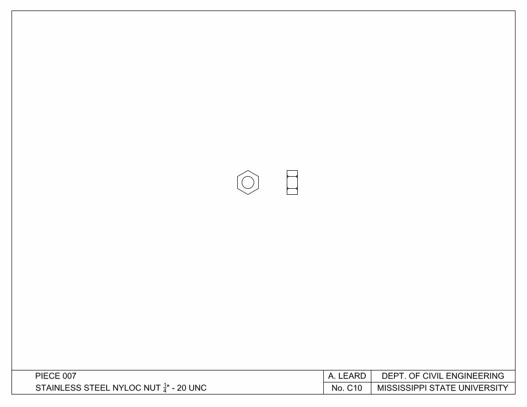
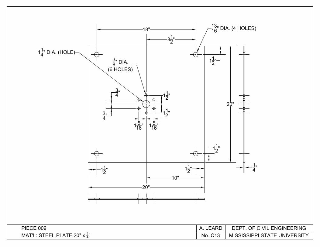
D1

APPENDIX D – MSP-LS PERMEATER DRAWINGS

Appendix D presents complete technical drawings for the MSP-LS permeameter. Within these drawings, there are five main assemblies. Each assembly is made up of various sub-assemblies and/or pieces. Assemblies and sub-assemblies are given a letter and number designation (e.g. assembly A-1 is the main assembly, A-2 and greater are sub-assemblies). Individual pieces are identified by piece numbers (P/N) (e.g. piece 001 or P/N 001). The five main assemblies for the MSP-LS are as follows:

1. The permeameter standpipe (Assembly A-1) 2. The permeameter test frame (Assembly B-1) 3. The surcharge load jack (Assembly C-1) 4. The load ring (Assembly D-1) 5. The water tray (Assembly E-1)

Evaluation of Approaches to Improve Longitudinal Joints in ...

Documents

Transcript of Evaluation of Approaches to Improve Longitudinal Joints in ...