
Evaluation of Algorithms for Land Cover Analysis using Hyperspectral Data
120
EVALUATION OF THE ALGORITHMS FOR LAND COVER ANALYSIS USING HYPERSPECTRAL DATA Technical Report 111 Evaluation of Algorithms for Land Cover Analysis using Hyperspectral Data Uttam Kumar 1 ([email protected]) Ramachandra T. V. 1 ([email protected]) Norman Kerle 2 ([email protected]) Clement Atzberger 2 ([email protected]) Milap Punia 3 ([email protected]) 1 Energy & Wetlands Research Group, Centre for Ecological Sciences, Indian Institute of Science, Bangalore – 560012. 2 International Institute of Geoinformation Science and Earth Observation, The Netherlands. 3 Indian Institute of Remote Sensing, Dehradun- 248001. Address for Correspondence: Dr. T.V. Ramachandra Energy & Wetlands Research Group Centre for Ecological Sciences Indian Institute of Science Bangalore 560 012, India E Mail: [email protected] [email protected] Tel: 91-080-2293 3099/ 2360985 Fax: 91-080-23601428 (CES-TVR) Web: http://ces.iisc.ernet.in/energy http://ces.iisc.ernet.in/grass 1
Transcript of Evaluation of Algorithms for Land Cover Analysis using Hyperspectral Data

EVALUATION OF THE ALGORITHMS FOR LAND COVER ANALYSIS USING HYPERSPECTRAL DATA
Technical Report 111
Evaluation of Algorithms for Land Cover Analysis using Hyperspectral Data
Uttam Kumar1 ([email protected]) Ramachandra T. V.1 ([email protected])
Norman Kerle2
([email protected]) Clement Atzberger2
([email protected]) Milap Punia3
1 Energy & Wetlands Research Group, Centre for Ecological Sciences, Indian Institute of Science, Bangalore – 560012.
2 International Institute of Geoinformation Science and Earth Observation, The Netherlands. 3 Indian Institute of Remote Sensing, Dehradun- 248001.
Address for Correspondence: Dr. T.V. Ramachandra Energy & Wetlands Research Group Centre for Ecological Sciences Indian Institute of Science Bangalore 560 012, India
E Mail: [email protected] [email protected] Tel: 91-080-2293 3099/ 2360985 Fax: 91-080-23601428 (CES-TVR) Web: http://ces.iisc.ernet.in/energy http://ces.iisc.ernet.in/grass
1

EVALUATION OF THE ALGORITHMS FOR LAND COVER ANALYSIS USING HYPERSPECTRAL DATA
Abstract Land cover is important for many planning and management activities and is considered an essential element for modelling and understanding the earth as a system. Land cover analysis relates to identifying the type of feature present on the surface of the earth. It deals with the identification of land cover features on the ground, whether vegetation, geologic, urban infrastructure, water, bare soil or others. Variations in land cover and its other physical characteristics influence weather and climate of our earth. Therefore the study of land cover plays an important role at the local/regional as well as global level for monitoring the dynamics associated with the earth. Land cover analysis has been done most effectively through satellite images of various spatial, spectral and temporal resolutions. Due to the spectral resolution limitations of conventional multispectral imageries, sensors that could collect numerous bands in precisely defined spectral regions were developed, leading to Hyperspectral Remote Sensing. Hyperspectral images have ample spectral information to identify and distinguish spectrally unique materials that allow more accurate and detailed information extraction. These imageries are classified into different land cover categories using various algorithms. The genesis and the underlying principle behind each of these algorithms are different and essentially produce land cover maps with varied accuracies. This report evaluates the utility of various classification algorithms for land cover mapping using MODIS data having high spectral resolution and coarse spatial resolution. NDVI (Normalised Difference Vegetation Index) was used to segregate the green (vegetation) and the non-green (non-vegetation) in the study area. Principal Component Analysis (PCA) and Minimum Noise Fraction (MNF) were used to reduce the data dimensionality and noise from the data. The hard classification algorithms used in this research include K-Means Clustering, Maximum Likelihood classification (MLC), Spectral Angle Mapper (SAM), Neural Network (NN) based classification, and Decision Tree Approach (DTA) to classify the image into 6 land cover classes (Agriculture, Built up (Urban / Rural), Evergreen / Semi-Evergreen forest, Plantations / orchards, Waste lands / Barren rock / Stony waste / Sheet rock and Waterbodies / Lakes / Ponds / Tanks / Wetland). The utility of a soft classification technique, Spectral unmixing using a Linear Mixture Model (LMM), was evaluated to calculate the proportions of the different land cover categories in a pixel. The endmembers, pure pixels or pixels with only one class within them, were identified using the Pixel Purity Index (PPI) and Scatter plot. These endmembers were used in spectral unmixing to yield abundance maps; a map indicating the proportion of each category within each pixel (fraction images). The accuracy of the MODIS classified maps were assessed by generating error matrix at the administrative boundary level (for Chikballapur Taluk) for which ground truth was collected from field. A comparative study of the percentage area for each land cover class for various classification algorithms was also done across all the taluks with the high spatial resolution LISS-3 MSS classified map as reference. At the pixel level, pixel to pixel analysis was done with respect to LISS-3 classified map. These results were also validated on the field. Results of this study show that NN on MNF components with an overall accuracy of 86.11%, and MLC on MODIS bands 1 to 7 with accuracy of 75.99% gave the best output among the various techniques. MLC on MODIS PC gave the lowest accuracy of 30.44%. The results are quite motivating for the application of land cover mapping using coarse spatial resolution data at a regional scale. Keywords: Land cover, Remote sensing, GIS, Hyperspectral data, MODIS, Multispectral data, algorithms, hard classification and soft classification
2

EVALUATION OF THE ALGORITHMS FOR LAND COVER ANALYSIS USING HYPERSPECTRAL DATA
Acknowledgements
We are grateful to Indian Space Research Organization – Indian Institute of Science – Space Technology Cell (ISRO – IISc – STC) and the Ministry of Envisonment and Forests, Government of India for the financial assistance. National Remote Sensing Agency (NRSA), Hyderabad and Global Land Cover Facility, NASA, USA provided the satellite data required for the study.
Address for Correspondence: Dr. T.V. Ramachandra Energy & Wetlands Research Group Centre for Ecological Sciences Indian Institute of Science Bangalore 560 012, India
E Mail: [email protected] [email protected] Tel: 91-080-2293 3099/ 2360985 Fax: 91-080-23601428 (CES-TVR) Web: http://ces.iisc.ernet.in/energy http://ces.iisc.ernet.in/grass
3

EVALUATION OF THE ALGORITHMS FOR LAND COVER ANALYSIS USING HYPERSPECTRAL DATA
Table of contents 1. Introduction ................................................................................................................................... 9
1.1. Land cover and Land use ......................................................................................................... 9 1.2. Hyperspectral Remote Sensing .............................................................................................. 11 1.3. Research Objectives ............................................................................................................... 14 1.4. Outline of the Report.............................................................................................................. 15 1.5. Data ........................................................................................................................................ 15
1.5.1. Instrument Background...................................................................................................... 15 1.6. Study Area.............................................................................................................................. 19
2. Preprocessing of Hyperspectral Image Data............................................................................. 21 2.1. The Challenges for Hyperspectral Processing........................................................................ 21
2.1.1. Calibration ......................................................................................................................... 21 2.1.2. Atmospheric Correction..................................................................................................... 21 2.1.3. Radiometric Correction...................................................................................................... 24 2.1.4. Data Normalisation ............................................................................................................ 25
2.2. Data Characteristics................................................................................................................ 26 2.2.1. Data Volume ...................................................................................................................... 26 2.2.2. Redundancy ....................................................................................................................... 26
2.3. Feature reduction / Band reduction / Data dimensionality reduction techniques ............................................................................................................................................ 26
2.3.1. Principal Component Analysis (PCA) ............................................................................... 26 2.3.2. Minimum Noise Fraction (MNF)....................................................................................... 27
3. Hard Classification Techniques.................................................................................................. 28 3.1. NDVI time series analysis ...................................................................................................... 28 3.2. Supervised Classification ....................................................................................................... 30
3.2.1. Gaussian Maximum Likelihood Classifier (GMLC) ......................................................... 30 3.2.2. Spectral Angle Mapper (SAM).......................................................................................... 32 3.2.3. Neural Network.................................................................................................................. 33 3.2.4. Decision Tree Approach .................................................................................................... 35
3.3. Unsupervised Classification ................................................................................................... 37 3.3.1. Clustering........................................................................................................................... 37 3.3.2. K – Means Algorithm ........................................................................................................ 38 3.3.3. Drawbacks of Clustering.................................................................................................... 39
3.4. Supervised versus Unsupervised Classification ..................................................................... 39 3.5. Validation of the result ........................................................................................................... 45
3.5.1. Classification Error Matrix ................................................................................................ 46 4. Soft Classification: Spectral Unmixing .......................................................................... 47
4.1. Introduction ............................................................................................................................ 47 4.2. Linear Unmixing .................................................................................................................... 48 4.3. Constraint Least Squares method (CLSM)............................................................................. 49 4.4. Endmember Extraction........................................................................................................... 49
4.4.1. Pixel Purity Index (PPI) ..................................................................................................... 50 4.4.2. Scatter Plot ......................................................................................................................... 51
4.5. Literature review: Spectral Unmixing.................................................................................... 51
4

EVALUATION OF THE ALGORITHMS FOR LAND COVER ANALYSIS USING HYPERSPECTRAL DATA
4.6. Summary ................................................................................................................................ 53 5. Results........................................................................................................................................... 55
5.1. Land cover Mapping using LISS-3 MSS ............................................................................... 55 5.1.1. Georeferencing and Geometric Correction ........................................................................ 55 5.1.2. Land Cover Analysis.......................................................................................................... 55
5.2. Land Cover Mapping using MODIS Data ............................................................................. 57 5.2.1. Georeferencing and Geometric Correction ........................................................................ 57 5.2.2. Land Cover Analysis.......................................................................................................... 57
5.3. Classification of high resolution LISS-3 MSS data ............................................................... 57 5.3.1. Unsupervised Classification............................................................................................... 58 5.3.2. Supervised Classification................................................................................................... 60
5.4. Classification of MODIS data ................................................................................................ 60 5.4.1. Classification of MODIS Bands 1 to 7 .............................................................................. 61 5.4.2. Classification of Principal Components (PC’s) of MODIS Bands 1 to 36 ........................ 66 5.4.3. Classification of Minimum Noise Fraction (MNF) components of MODIS Bands 1 to 36 70
5.5. Soft classification: Spectral Unmixing of MODIS imagery................................................... 74 5.5.1. MNF Transformation ......................................................................................................... 74 5.5.2. Endmember collection ....................................................................................................... 74 5.5.3. Class spectral characteristics of the Endmembers.............................................................. 75 5.5.4. Linear Spectral Unmixing.................................................................................................. 76
6. Accuracy Assessment................................................................................................................... 80 6.1. LISS-3 MSS Classification Accuracy .................................................................................... 80 6.2. MODIS Classification Accuracy............................................................................................ 82
6.2.1. Accuracy Assessment of hard classification for MODIS................................................... 82 6.2.2. Accuracy Assessment of Soft classification for MODIS................................................... 88
6.3. Discussion .............................................................................................................................. 89 6.3.1. Hard Classification............................................................................................................. 89 6.3.2. Soft Classification using Linear Spectral Unmixing.......................................................... 89 6.3.3. Classification Accuracy ..................................................................................................... 90
7. Conclusions................................................................................................................................... 91 8. References..................................................................................................................................... 94 Annexure A ........................................................................................................................................ 103
L1B Reflective Calibration - The MODIS reflective calibration algorithm is designed to determine the at-aperture spectral radiance of the Earth scene and the bidirectional reflectance of the Earth scene with their respective associated uncertainties. Level 1A data is Earth-located raw sensor digital numbers and Level 1B data is Earth-located, calibrated data in physical units. The Solar Diffuser, Spectroradiometric Calibration Assembly (SRCA) and Space View are used periodically to determine calibration coefficients for the reflective bands. The Space View is used every scan along with the periodic calibration results to calibrate the reflective bands. The on-orbit reflective band calibration is a one-point method adjusted by data from a two-point periodic method to fit a linear detector response [2]............................................................................................................ 103
Annexure B......................................................................................................................................... 107 Similarity Metrics and Clustering Criteria..................................................................................... 108 Automatic Cluster Detection ......................................................................................................... 109
Annexure C ........................................................................................................................................ 110
5

EVALUATION OF THE ALGORITHMS FOR LAND COVER ANALYSIS USING HYPERSPECTRAL DATA
Annexure D ........................................................................................................................................ 113
List of figures Figure 1.1: Study area – Kolar district, Karnataka State, India ............................................................... 19 Figure 2.1: Atmospheric effects influencing the measurement of reflected solar energy…………... 22 Figure 2.2: Atmospheric correction processing thread flow chart [49]. ................................................ 24 Figure 2.3: Rotated coordinate axes in PCA ......................................................................................... 27 Figure 3.1: Equiprobability contours defined by a maximum-likelihood classifier. ............................... 31 Figure 3.2: Spectral Angle Mapping concept. (a) For a given feature type, the vector corresponding to
its spectrum will lie along a line passing through the origin, with the magnitude of the vector being smaller (A) or larger (B) under lower or higher illumination, respectively. (b) When comparing the vector for an unknown feature type (C) to a known material with laboratory-measured spectral vector (D), the two features match if the angle ‘α’ is smaller than a specified tolerance value. (After Kruse et al., 1993) [34]. ........................................................................................................ 32
Figure 3.3: Example of an artificial neural network with one input layer, two hidden layers and one output layer [19]. ............................................................................................................................. 34
Figure 3.4: Example of Decision Tree..................................................................................................... 36 Figure 3.5: LISS-3 Preprocessing and Classification. ............................................................................. 44 Figure 3.6: Processing and Hard Classification of MODIS data. ............................................................ 45 Figure 4.1: Four cases of mixed pixels [116]. ......................................................................................... 48 Figure 4.2: Scatter plots between two bands typically show a triangular shape, with the data radiating
away from the shade-point and A, B, C as the endmembers. .......................................................... 51 Figure 4.3: Overall methodology of linear unmixing process. ................................................................ 54 Figure 5.1: NDVI of LISS-3 MSS based on bands 3 (Red) and 4 (NIR). ............................................... 56 Figure 5.2: NDVI generated using MODIS bands 1 and 2...................................................................... 56 Figure 5.3: Unsupervised classification of LISS-3 image. ...................................................................... 58 Figure 5.4: (A) False Colour Composite of the LISS-3 image, (B) Kolar district with training data set,
(C) Supervised Classified image of LISS-3 MSS............................................................................ 59 Figure 5.5: Different MODIS inputs to the hard classification algorithms. ............................................ 61 Figure 5.6: Unsupervised Classification on MODIS Bands 1 to 7. ......................................................... 62 Figure 5.7: Plot of training RMS vs. iterations of NN applied on MODIS bands 1 to 7......................... 63 Figure 5.8: Supervised Classification using (A) MLC, (B) SAM, (C) NN and (D) Decision Tree
Approach on MODIS Bands 1 to 7.................................................................................................. 65 Figure 5.9: Plot of training RMS vs. iterations of NN applied on PCA bands (MODIS Bands 1 to 36).67Figure 5.10: Supervised Classification using (A) MLC, (B) SAM, (C) NN and (D) Decision Tree
Approach on PC’s............................................................................................................................ 69 Figure 5.11: Plot of training RMS vs. iterations of NN applied on MNF Components. ......................... 71 Figure 5.12: Supervised Classification using (A) MLC, (B) SAM, (C) NN and (D) Decision Tree
Approach on MNF components....................................................................................................... 73 Figure 5.13: 3-Dimensional visualisation of the Endmembers showing their separability. .................... 76 Figure 5. 14: (A) Gray scale Abundance Maps for Agriculture and (B) Built up land (Urban / Rural).. 77
6

EVALUATION OF THE ALGORITHMS FOR LAND COVER ANALYSIS USING HYPERSPECTRAL DATA
Figure 5.15: Gray scale Abundance Maps for Evergreen / Semi-Evergreen Forest (A) Plantations/orchards (B) Wasteland/Barren rock/Stone (C) and Waterbodies (D). Bright pixels represent higher abundance of 50% or more stretched from black to white.................................... 78
Figure 5.16: Overall RMSE for MODIS. Bright pixels represent high error. ......................................... 79 Figure 6.1: Chikballapur taluk in Kolar district where field data were collected.................................... 81 Figure 6.2: Best (left) to worst (right) classification algorithms for mapping land cover classes in
Chikballapur taluk. LISS-3 MSS classified image is used for comparison. .................................... 85
7

EVALUATION OF THE ALGORITHMS FOR LAND COVER ANALYSIS USING HYPERSPECTRAL DATA
List of tables Table 1.1: Specifications of MODIS sensor [19]..................................................................................... 17
able 3.1: Genesis, advantages and the disadvantages of the classification techniques. ........................ 43 T Table 5.1: Transformed Divergence matrix of the spectral classes in LISS-3. Values greater than 1.9
indicate a very good separability. .................................................................................................... 58 Table 5.2: Class wise percentage statistics for Unsupervised and Supervised classified maps using
LISS-3 MSS..................................................................................................................................... 60 Table 5.3: Transformed Divergence matrix of the spectral classes in MODIS Bands 1 to 7. ................. 61 Table 5.4: Knowledge based Land cover classification of MODIS data (Bands 1 to 7). ........................ 64 Table 5.5: Percentage wise distribution of land cover classes for MODIS bands 1 to 7 classified using
K-Means, MLC, SAM, NN and Decision Tree Approach. ............................................................. 64 Table 5.6: Eigenvalue for the PCA analysis of MODIS 36 bands. ......................................................... 66 Table 5.7: Transformed Divergence matrix of the spectral classes in PCs.............................................. 66 Table 5.8: Knowledge based LC classification of PC’s. ......................................................................... 67 Table 5.9: Percentage wise distribution of LC using MLC, SAM, NN and DTA on PC’s. .................... 68 Table 5.10: Eigenvalue for the MNF analysis of MODIS 36 bands........................................................ 70 Table 5.11: Transformed Divergence matrix of the spectral classes in MNF. ........................................ 70 Table 5.12: Knowledge based LC classification for MNF components. ................................................. 71 Table 5.13: Percentage wise distribution of LC classes obtained from MNF components classification
using MLC, SAM, NN and DTA..................................................................................................... 72 Table 5.14: Land cover classes compared on the basis of different algorithms versus percentage area. 74 Table 6.1: Area statistics of each taluk in Kolar district.......................................................................... 81 Table 6.2: Producer’s accuracy, user’s accuracy and overall accuracy of land cover classification using
LISS-3 MSS data for Chikballapur Taluk. ...................................................................................... 81 Table 6.3: Overall Accuracy of classified MODIS Data of Chikballapur taluk. ..................................... 82 Table 6.4: User’s Accuracy of classified MODIS Data of Chikballapur taluk........................................ 82 Table 6.5: Producer’s Accuracy of classified MODIS Data of Chikballapur taluk................................. 83 Table 6.6: Land Cover statistics for Chikballapur Taluk.................................................................. 83 Table 6.7: Overall Accuracy obtained from pixel to pixel analysis with LISS-3 image comparison for
Chikballapur Taluk. ......................................................................................................................... 86 Table 6.8: User’s Accuracy obtained from pixel to pixel analysis with LISS-3 image comparison for
Chikballapur taluk. .......................................................................................................................... 87 Table 6.9: Producer’s Accuracy obtained from pixel to pixel analysis with LISS-3 image comparison
for Chikballapur taluk...................................................................................................................... 87 Table 6.10: Land Cover details of fraction images for Chikballapur taluk. ............................................ 88 Table 6. 11: Validation of land cover classes in Chikballapur. ............................................................... 88
8

EVALUATION OF THE ALGORITHMS FOR LAND COVER ANALYSIS USING HYPERSPECTRAL DATA
1. Introduction
Land cover describes the physical state of the earth’s surface and immediate surface in terms of the natural environment (such as vegetation, soils, earth’s surfaces and ground water) and the man-made structures (e.g. buildings). These land cover features have been classified using the remotely sensed satellite imagery of different spatial, spectral and temporal resolutions. Land cover analysis using high spectral resolution has several advantages, since it aids in numerous mapping applications such as soil types, species discrimination, mineral mapping etc. “Hyperspectral data” having numerous contiguous bands has high spectral resolution. Hyperspectral data processing possesses both challenges and opportunities for land cover mapping. Land cover mapping can be performed using various algorithms by processing the remotely sensed data into different themes or classes. The present research aims at comparing the results obtained from various classification algorithms using hyperspectral data for land cover mapping.
1.1. Land cover and Land use
Land cover refers to what is actually present on the ground and may also contain an ecological description. It provides the ground cover information for baseline thematic maps. In contrast, land use refers to the various applications and the context of its use. Land use itself is the human employment of a land-cover type. It involves both the manner in which the biophysical attributes of the land are manipulated and the intent underlying that manipulation, the purpose for which the land is used. Identifying, delineating and mapping land cover on temporal scale provides an opportunity to monitor the changes, which is important for natural resource management and planning activities. Land cover changes induced by human and natural processes play a major role in global as well as at regional scale patterns of the climate, hydrology and biogeochemistry of the earth system. Although the oceans are the major driving force for the earth’s physical climatology, the land surface has considerable control on the planet’s biogeochemical cycles, which in turn significantly influence the regional climate system through the radiative properties of green house gases and reactive species [1]. Terrestrial ecosystems exert considerable control on the planet’s biogeochemical cycles, which in turn significantly influence the climate system [2]. Further, variations in topography, vegetation cover and other physical characteristics of the land surface influence surface-atmosphere fluxes of sensible heat, latent heat, and momentum, which in turn influence weather and climate [3]. Land cover mapping employing moderate to coarse resolution datasets often in tandem with ancillary databases have been reported from different parts of the world at regional scale. The National Mapping program, a component of the U.S. Geological Survey (USGS), mapped land cover of the United States based on aerial photography acquired by NASA (National Aeronautics and Space Administration) and the USGS during 1970’s and 1980’s. The data were manually interpreted and land cover polygons were compiled onto 1:250, 000 base USGS maps. The Anderson hierarchical scheme used with this data had nine categories and several detailed level 2 classes [4]. Compilation of a 1:1 million scale atlas of Land cover Map as a first hand map for 1991 covering the entire territory of China was done based on field surveys, satellite images and aerial photos; classes were regrouped into 20 major land-use/land cover classes in the digital map [5]. Another database of China, the “Temperate East Asia Land-Cover Database (TEAL)” used 1992 NOAA (National Oceanic & Atmospheric Administration)-AVHRR (Advanced Very High Resolution Radiometer) 1-km remote sensing information and existing land cover maps developed using traditional and geographical techniques that involved extensive manual survey, data keeping, database preparation and developing maps using cartographical techniques. The database was developed to understand the land cover change in East China [4].
9

EVALUATION OF THE ALGORITHMS FOR LAND COVER ANALYSIS USING HYPERSPECTRAL DATA
The National Land Cover Database (NLC) of South Africa provides a standardised land cover database for South Africa, Swaziland and Lesotho. The land cover database was derived (using manual photo-interpretation technique) from a series of 1:250,000 scale geo-rectified on seasonally standardised, single date LANDSAT THEMATIC Mapper TM satellite imagery captured principally during the period 1994-95 [4]. The Global Vegetation Monitoring unit of the JRC, ISPRA, Italy has produced a new global land cover classification for the year 2000, in collaboration with over 30 research teams from around the world. The project was carried out to provide accurate baseline land cover information, a harmonized land cover database over the whole globe and presented at the International Convention on Climate Change, the Convention to Combat Desertification, the Kyoto Protocol etc. GLC, 2000 dataset is a main input dataset to define the boundaries between ecosystems such as forest, grassland, and cultivated systems. In this project, more than 30 research teams were involved, contributing to 19 regional windows. Each defined region was mapped by local experts, which guaranteed an accurate classification, based on local knowledge. The mosaicing of 21 regional products, and the translation to a standardised global legend, made it possible to create a consistent global land cover classification based on regional expert knowledge. In contrast to former global mapping initiatives, the GLC, 2000 project is a bottom up approach to global mapping [4]. Recent exercise of National Land Cover Database for the United States known as “Multiresolution Land Characterisation 2001 (MRLC 2001)” has attempted to create an updated pool of Landsat 5 and 7 data to generate land cover database (National Land Cover Database 2001). The efforts covered aspects of providing consistent land cover database as well as to provide a portable data framework useful in several applications. The database included satellite images, elevation model and terrain products, per pixel estimates of percent imperviousness, percent tree canopy and 29 land cover classes [4]. Another recent attempt on global LULC (Land Use Land Cover) for vegetation mapping was the use of MODIS data as one of the most critical global data sets. The classification included 17 categories of land cover following the International Geosphere-Biosphere Program (IGBP) scheme. The set of cover types includes eleven categories of natural vegetation covers broken down by life form; three classes of developed and mosaic lands, and three classes of non-vegetated lands [4]. The Global Land Cover Facility (GLCF) provides land cover from the local to global scales to understand global environmental systems. GLCF research focuses on determining land cover and land cover change around the globe. In particular, the GLCF develops and distributes remotely sensed satellite data and products that explain land cover from the local to global scales. The data provided by GLCF can prove useful in global, regional and even local analyses of the earth's surface. These 1km global land cover product can be particularly useful when combined with higher resolution data types such as Landsat TM, ETM+ and MSS [6]. Global land cover classification using coarse resolution data was carried out from 1991 through August 1997 supported by NASA's Terrestrial Ecology Program on Land Cover Land Use Change (TEP-LCLUC) for mapping global land cover from satellite data, with the aim of improving the accuracy of land cover data sets and to parameterize global change models. These efforts have produced a global land cover data set at one-degree spatial resolution [7], [8] based on a maximum likelihood classification of annual NDVI temporal profiles. The CORINE land cover map is the European Union standard dataset for land cover applications; it is available for national as well as for international applications for European and accession countries. The CORINE Land cover map includes 44 land cover/land use classes divided into 5 main categories (agricultural areas, artificial surfaces, forests & semi natural areas, wetlands and waterbodies). Besides the classes on paved areas, agricultural areas, forest areas and water/wet lands, other categories include land cover 10 classes important in terms of nature and landscape protection. The inventory is based primarily on satellite scenes of Landsat (4, 5 and 7) TM data of different vegetation periods with
10

EVALUATION OF THE ALGORITHMS FOR LAND COVER ANALYSIS USING HYPERSPECTRAL DATA
additional information in the form of topographic maps and orthogonal photos. To fulfill European and national requirements in an appropriate way, the member countries are in the process of defining a level 4 CORINE classification with detailed descriptions for some of the 44 land cover classes. The European wide raster data sets at 250 x 250 m and 1x1 km² resolutions were derived from the national vector data base at a scale of 1:100,000. Areas with a minimum size of 25 ha and rivers and transport routes of a minimum width of 100 m were detected and mapped into the geographical information system. The first inventory started in the 1990 and the first update was carried out within a common 20 and was finished in 2003. The method instructs countries to detect land use changes from a minimum of 5 ha areas and line elements from a 100 m width [9]. In India, land use and land cover (LULC), an important study from national perspective on annual basis using data from the latest Indian Remote Sensing Satellite – Resourcesat has been initiated by ISRO (Indian Space Research Organisation) and NRSA (National Remote Sensing Agency), Department of Space in coordination with several RRSSCs (Regional Remote Sensing Service Centres). Spatial accounting and monitoring of land use and land cover systems (like agriculture, surface waterbodies, waste lands, forests, etc.) was carried out on a national level on 1:250,000 scale using multi-temporal IRS (Indian Remote Sensing Satellites) AWiFS (Advanced Wide Field Sensor) datasets to provide on annual basis, net sown area for different cropping seasons and integrated LULC map. The AWifs data covered Kharif (August – October), Rabi (January – March) and Zaid (April – May) seasons to address spatial and temporal variability in cropping pattern and other land cover classes. Decision tree classifier method was adopted to account the variability of temporal datasets and bring out reliable classification outputs. Legacy datasets on forest cover, type, wastelands and limited ground truth were used as inputs for classification and accuracy assessment [4]. This highlights, the numerous efforts made till date with various multisensor data having different spatial, spectral and temporal resolutions for land cover mapping using different algorithms around the globe. However, these studies do not reflect the technique that yields the best land cover map and it still remains a subject for research. A study on comparative evaluation of classification algorithms using hyperspectral data would entail a useful accurate result for future land cover mapping applications.
1.2. Hyperspectral Remote Sensing
Due to the spectral resolution limitations of conventional multispectral remote sensing, in the 1980’s, the Jet Propulsion Laboratory (JPL) with NASA took up an initative to develop instruments that could create images of earth’s surface at unprecedented levels of spectral details. Whereas previous multispectral sensors collected data in a few rather broadly defined spectral regions, these new instruments could collect 200 or more very precisely defined spectral regions. These instruments created the field of “Hyperspectral Remote Sensing”. EOS (Earth Observing System) is the centerpiece of NASA’s Earth Science mission. The EOS AM-1 satellite, later renamed Terra, is the flagship of the fleet and was launched in December 1999. It carries five remote sensing instruments, including the MODIS and the Advanced Spaceborne Thermal Emission and Reflectance Radiometer (ASTER) [15]. Moderate Resolution Imaging Spectroradiometer (MODIS) is a major instrument on the Earth observing System EOS-AM1 and EOS-PM1 (termed AQUA) missions [16]. The “heritage” of the MODIS comes from several space-borne instruments. These include the Advanced Very High Resolution Radiometer (AVHRR), the High Resolution Infrared Sounder (HIRS) unit on the National Oceanic and Atmospheric Administration’s (NOAA) Polar Orbiting Operational Environmental Satellites (POES), the Nimbus-7 Coastal Zone Colour Scanner (CZCS), and the Landsat Thematic Mapper (TM). MODIS is able to continue and extend the databases acquired over many years by the AVHRR, in particular, and the CZCS/Sea Star-Sea WiFS series. The “Hyper” in hyperspectral means “too many” and refers to the large number of measured wavelength bands. Hyperspectral images are spectrally over determined, which means that they provide
11

EVALUATION OF THE ALGORITHMS FOR LAND COVER ANALYSIS USING HYPERSPECTRAL DATA
ample spectral information to identify and distinguish spectrally unique materials. Hyperspectral imagery provides the potential for more accurate and detailed information extraction than is possible with any other type of conventional remotely sensed data. Hyperspectral data set can be visualized as a three dimensional cube, with two dimensions represented by the spatial coordinates, while third dimension is represented by the spectral bands. Hyperspectral remote sensing is also known as the “Imaging Spectroscopy” as it works on the principle of Spectroscopy. Spectroscopy is the technique of producing spectra, analyzing their constituent wavelength, and using them for chemical or physical analysis or the determination of energy levels and molecular structure. A spectrum is formed by the emission or by absorption of electromagnetic radiation accompanying change between the energy levels of atoms and molecules. The frequency of reflection or radiation depends upon the type of energy levels involved and hence the type of surface and material being observed. Hyperspectral imagery has been used to detect and map a wide variety of materials having characteristic reflectance spectra. For example, hyperspectral images have been used by geologists for mineral mapping [10], and to detect soil properties including moisture, organic content, and salinity [11]. Vegetation scientists have successfully used hyperspectral imagery to identify vegetation species [12], [13] and [14]. Remote sensing has been used as a basis for mapping global land cover using data from multispectral remote sensing sensors, for example, the Advanced Very High Resolution Radiometer (AVHRR). Land cover identification establishes the baseline data from which resource monitoring and management can be performed. Nowadays the demand of accurate land cover maps is increasing in order to address the global issues such as global warming, land degradation and water scarcity [2]. These kinds of databases are primary important for national accounting of natural resources and planning at regular intervals. Land use and Land cover mapping using satellite remote sensing data can provide a reliable database to assess the status of natural resources. The advances in geo-informatics coupled with the availability of higher spatial, spectral and temporal resolution data has helped to investigate and model the environmental systems for maintaining the ecological sustainability. In this context, an important application of accurate global land-cover information is the inference of parameters that influence biophysical processes and energy exchanges between the atmosphere and the land surface as required by regional and global-scale climate and ecosystem process models [17]. Until recently, land cover data sets used within different models (e.g., global climate and biogeochemistry) were derived from pre-existing maps and atlas. While these data sources provided the best available source of information regarding the distribution of land cover at the time, several limitations are inherent in their use. For example, land cover is intrinsically dynamic. Therefore, the source data upon which these maps were compiled is now out of date in most areas. Also conventional land cover data sets, such as those mentioned above, often provide maps of potential vegetation inferred from climatic variables such as temperature and precipitation. In many regions, especially where humans have dramatically modified the landscape, the true vegetation type or land cover can deviate significantly from the potential vegetation. MODIS, on-board the Terra platform, includes seven spectral bands that are explicitly designed for “land cover applications”. The enhanced spectral, radiometric, and geometric quality of MODIS data provides a greatly improved basis for mapping global land cover relative to earlier remote sensing data. MODIS data are also freely available via ftp through the EOS Data Gateway http://glcf.umiacs.umd.edu/data. This enables land cover mapping at the national/regional level economically. There are many techniques for mapping land cover using the remotely sensed data viz. hard and soft classification algorithms. For example, the first global land cover map compiled from remote sensing was produced [18] using maximum likelihood classification of monthly composite AVHRR normalized difference vegetation index (NDVI) data at 1 degree spatial resolution. In particular, when using
12

EVALUATION OF THE ALGORITHMS FOR LAND COVER ANALYSIS USING HYPERSPECTRAL DATA
computer-assisted classification methods, it is frequently not possible to map consistently at a single level of classification hierarchy. This is typically due to the occasionally ambiguous relationship between land cover and spectral response and the implications of land use on land cover [19]. The use of different algorithms for land cover classification also depends on the data and the application in hand. The principle and the purpose behind each of these techniques may be different and each of these algorithms may result in different output maps. Hence, the focus of this research is to evaluate a range of existing classification algorithms (hard and soft) for land cover mapping in Kolar district, Karnataka, India using MODIS data with respect to high resolution LISS-3 (Linear Imaging Self Scanner) MSS classified image and detailed ground truth data. Consequently and conceptually, this research framework aims at developing an algorithm that classifies the MODIS data into different predetermined land cover classes more accurately with better results. Prior to the availability of newer, high quality data sets from instruments onboard the Terra (and other) space craft, data sets derived from the AVHRR (Advanced Very High Resolution Radiometer) provided the best available remote sensing based maps of global land cover. However, because the information content of AVHRR data is limited, numerous uncertainties are present in these maps for land cover mapping applications [20]. MODIS data with better spectral resolution have a spatial resolution of 250 m, 500 m and 1 km. Several hard and soft classification techniques exist for land cover classification. The hard classification techniques for example, Maximum Likelihood classification (MLC), Spectral Angle Mapper (SAM), Neural Network (NN) based classification, Normalized Difference Vegetation Index (NDVI) and Clustering technique classify the image on a pixel-basis into different categories. These algorithms automatically categories all pixels in an image into land cover classes or themes. The spectral pattern present within the data for each pixel is used to perform the classification and, indeed, the spectral pattern present within the data for each pixel is used as the numerical basis for categorization [19]. Nevertheless, MODIS pixels, having coarse spatial resolution, contain more than one class or endmember in a single pixel, called mixed pixel, covering more than one land cover type, as is present in reality due to the heterogeneous presence of features on the earth’s surface. Therefore unmixing of these mixed pixels is required for estimation of individual class representation in the pixel. Spectral unmixing is generally described as a quantitative analysis procedure used to recognize constituent ground cover materials (or endmembers) and obtain their mixing proportions (or abundances) from a mixed pixel. That is, the sub-pixel information of endmembers and their abundances can be obtained through the spectral unmixing process. Therefore, land cover mapping can be carried out at a sub-pixel level. The spectral unmixing problem has caused concerns and has been investigated extensively for the past two decades. A general analysis approach for spectral unmixing is first to build a mathematical model of the spectral mixture. Then, based on the mathematical model, certain techniques are applied to implement spectral unmixing. In general, mathematical models for spectral unmixing are divided into two broad categories: linear mixture model (LMM) and nonlinear mixture models (NLMM). The LMM assumes that each ground cover material only produces a single radiance, and the mixed spectrum is a linear combination of ground cover radiance spectra. The NLMM takes into account the multiple radiances of the ground cover materials, and thus the mixture is no longer linear. The NLMM typically has a relatively more accurate simulation of physical phenomena, but the model is usually complicated and application dependent. Typically there is not a simple and generic NLMM that can be utilized in various spectral unmixing applications. This disadvantage of the NLMM greatly limits its extensive application. In contrast, the LMM is simpler and more generic, and it has been proven successful in various remote sensing applications, such as geological applications [21], forest studies [22], [23], [24], and vegetation
13

EVALUATION OF THE ALGORITHMS FOR LAND COVER ANALYSIS USING HYPERSPECTRAL DATA
studies [25]. For example, [21] utilized the LMM to determine the mineral types and abundances. Using the LMM, [22] estimated the proportions of forest cover in regions with small forest patches and convoluted clearance patterns; [23] determined the forest species and canopy closure for forest ecological studies and forest management. It is because of the advantage of simplicity and generality that the LMM has become a dominant mathematical model for the spectral unmixing analysis. Another major reason why the LMM has been broadly accepted for the spectral unmixing analysis is that the linear mixture assumption allows many mature mathematical skills and algorithms, such as least squares estimation (LSE) [26], [27], to be easily applied to the spectral unmixing problem. One requirement for implementing the abundance estimation using the LSE method is that the number of spectral bands must be greater than the number of endmembers. This is called the “condition of identifiability” [28]. To a certain extent, the “condition of identifiability” limits the use of multispectral data for the linear spectral unmixing problem. Multispectral data typically have only a few spectral bands. Thus, when the number of endmembers increases, the “condition of identifiability” no longer holds and the LSE method fails. One solution to this problem is to utilise hyperspectral data, which typically have high number of spectral bands (MODIS - 36 Bands). The problem of “condition of identifiability” seems to be easily solved by utilizing hyperspectral data.
1.3. Research Objectives
India is bestowed with valuable natural resources consisting of forests, mineral deposits, wetlands, rivers, surface waterbodies and vast areas of agriculture serving the needs of around a billion population and varied ecological functions. Studies so far conducted in India are limited in scope, as they only cater for the base line data towards regional planning and evaluations. The national spatial database enabling the monitoring of temporal dynamics of agricultural ecosystems, forest conversions, and surface waterbodies etc are lacking and the latest maps do not account for the gaps in updated information [4]. In India, the information on LC in the form of thematic maps, records and statistical figures is inadequate and does not provide up to date information on the changing land use patterns and processes. Although, over the years, there has been substantial efforts made by various Central/State Government Departments, Institutions/ Organisation etc. to account for the national repository, yet they have been sporadic and efforts are often duplicated. In most of the cases, as the time gap between reporting, collection and availability of data is large, the data often become out-dated [4]. Realizing the need for an up to date nationwide land cover pattern, the present research on evaluation of the algorithms for land cover analysis can be beneficial and useful for defining a proper methodology. The main objective of this work is to evaluate different hard and soft classification algorithms using mono-temporal MODIS sensor data for better land cover (Agriculture, Built up (Urban / Rural), Evergreen / Semi-Evergreen forest, Plantations / orchards, Waste lands / Barren rock/ Stony waste / Sheet rock and Waterbodies / Lakes / Ponds / Tanks / Wetland) mapping. MODIS and the IRS LISS 3 data are properly registered and resampled that are cloud-screened and atmospherically corrected and two data sets have the same projection and coordinate system. An attempt was made to address the following:
1. What are the utility / usefulness of the existing hard classification techniques for land cover mapping at regional scale using MODIS data?
2. What is the effect of different pre-processing techniques on the accuracy of different hard
classification algorithms?
3. How to extract the end members directly from the data without using existing spectral libraries?
14

EVALUATION OF THE ALGORITHMS FOR LAND COVER ANALYSIS USING HYPERSPECTRAL DATA
4. What is the utility of spectral unmixing model to obtain the abundance maps of the different interpretable classes?
5. What is the effect of different spatial scales on classification accuracy?
6. Which hard/soft classification approach yields the best land cover mapping results?
The evaluation of different algorithms for better land cover mapping envisages the need of the natural resources database depository. This study is based on all the 36 bands of MODIS data, and the land cover categories being considered are agriculture, built up, forest, plantation, barren/rocky/stony/waste land and waterbodies which are the dominating classes in the study area.
1.4. Outline of the Report
The report is organised in seven chapters. First chapter introduces the basic concepts of hyperspectral remote sensing, while the second chapter describes the steps of preprocessing the hyperspectral image data. The third chapter discusses the commonly used Normalised Difference Vegetation Index (NDVI) and deals with the hard classification algorithms for land cover mapping in detail: K-means Clustering, Maximum Likelihood Classification (MLC), Spectral Angle Mapper (SAM), Neural Network (NN) and the Decision Tree Approach (DTA). The fourth chapter highlights the soft classification technique. It includes the Linear Mixture Model (LMM), endmember selection and estimation of proportion of the endmembers. The fifth chapter describes the results after implementing the different classification algorithms. This chapter also describes the comparison of results obtained within and between the different classification algorithms (hard and soft). Evaluation of the results obtained from different classification algorithms are performed at two spatial scales; the administrative boundary (Taluk) and the pixel level, and is discussed in the sixth chapter. Use of training sites in validation along with the sources of error and uncertainty are also discussed here.
1.5. Data
1.5.1. Instrument Background
MODIS was originally conceived as a system composed of two instruments called MODIS-N (nadir) and MODIS-T (tilt), which were slated for flight on the EOS-AM platforms. These two instruments were described in various levels of detail in studies as far back as 1985 [29]. MODIS-T was designed basically as an advanced ocean colour sensor with the ability to tilt, to avoid sun glint. The MODIS-T instrument was eventually removed from further development as the budget for EOS became more constrained. In order to minimize the impact of the loss of MODIS-T and meet or approach other scientific objectives that were not being met at that time, such as observations of the diurnal variation in the earth’s cloudiness, MODIS-N was also placed on the EOS-PM1 platforms. This enabled morning and afternoon observations to be obtained. The two MODIS instruments could, in combination, obtain more ocean colour coverage than one (e.g., one MODIS on the EOS-AM1 mission) could (i.e., reduce data loss due to sun glint), but not as much as MODIS-N and MODIS-T on one platform. As the result of the loss of MODIS-T, MODIS-N was simply called MODIS. However, between 1989 and 1998, the original concept for MODIS-N experienced several changes, including the number and placement of bands for the instrument. The 40-band instrument envisioned in 1989 is reduced to a 36-band instrument. Within the 36 bands on MODIS, there are three major band segments. The first seven bands are used to observe land cover features plus cloud and aerosol properties [30], [31] (bands numbered 1-7 in Table: 1.1 [19]). The spectral placements of these bands are derived so as to be very similar to the bands on the Landsat TM, albeit the spatial resolutions are 250 or 500 m, depending on the MODIS band involved. There are nine ocean colour bands (bands 8-16) that are derived from the studies leading to the Nimbus CZCS and the SeaWiFS instrument. Another set of bands (bands 20-25 and 27-36) is modelled after the
15

EVALUATION OF THE ALGORITHMS FOR LAND COVER ANALYSIS USING HYPERSPECTRAL DATA
bands of the HIRS, with emphasis on those HIRS bands that sense properties of the troposphere and the surface. In the original concept for the MODIS-N, there were three bands near 700 nm to measure polarization that were dropped along with three bands near 760 nm to observe optical properties of clouds in the oxygen-A band absorption region. These were replaced by one broad and two narrow bands near 900 nm (bands 17-19 in Table: 1.1) that were derived from analyses of data from the airborne AVIRIS instrument. These bands enable water-vapour observations in the lower troposphere as well as some cloud properties. There was a need to make further reductions in the predicted overall cost of the MODIS so two separate 250 m spatial resolution bands at 575 and 880 nm were combined with two 500 m bands at roughly the same centre wavelengths. This resulted in a compromise (bands 1 and 2), whereby the 250 m spatial resolution was retained but with 50 and 35 nm bandwidths that were somewhat broader than the bandwidths associated with the original 500 m bands. Finally, more analyses of the AVIRIS data indicated high value in gathering cirrus cloud observations by adding a band at 1.38 µm. To keep the number of MODIS bands limited to no more than 36, it was decided to replace a 3.959 µm atmospheric sounding band (band 26) with the 1.38 µm capability. The MODIS instrument sees the entire surface of the Earth every 1-2 days. MODIS has a good temporal repeativity twice a day (using both Terra MODIS and Aqua MODIS) [32], [33]. Data is acquired in contiguous scans of swath width (2330 km) across track and 10 km along track to provide 2-day repeat observations of the Earth with a repeat orbit pattern every 16 days. Each earth scene collected by the MODIS is sampled 1354 times over a range of principal scan angles of -55 to +55 degree. All samples are co-registered in the sensor data system as frames and telemetered together to the ground. At nadir, a frame is 10,000 m in extent in the track direction and 1000 m extent in the scan direction (orthogonal to spacecraft orbital direction). It has 12-bit radiometric sensitivity. In addition, MODIS data are characterized by improved geometric rectification and radiometric calibration. Band-to-band registration for all 36 MODIS channels is specified to be 0.1 pixel or better. The 20 reflected solar bands are absolutely calibrated radiometrically with an accuracy of 5 percent or better. The calibrated accuracy of the 16 thermal bands is specified to be 1 percent or better. These stringent calibration standards are a consequence of the EOS/ESE requirement for a long term continuous series of observations aimed at documenting subtle changes in global climate [19]. As mentioned earlier, for this research work MODIS data, downloaded from the Earth Observing System Data Gateway [34] has been used for the land cover mapping. These data sets are known as “MOD 09 Surface Reflectance 8-day L3 global” product at 250 (band 1 and band 2) and 500m (band 1 to band 7). The MODIS Surface-Reflectance Product (MOD 09) is computed from the MODIS Level 1B land bands 1, 2, 3, 4, 5, 6, and 7 (centered at 648 nm, 858 nm, 470 nm, 555 nm, 1240 nm, 1640 nm, and 2130 nm, respectively). The product is an estimate of the surface spectral reflectance for each band as it would have been measured at ground level if there were no atmospheric scattering or absorption [35]. Each MODIS Level-1B data product [36], contains the radiometrically corrected, fully calibrated and geolocated radiances at-aperture for all 36 MODIS spectral bands at 1km resolution [37]. These data are broken into granules approximately 5-min long and stored in Hierarchical Data Format (HDF). Band 1 to band 36 MODIS data “MOD 02 Level-1B Calibrated Geolocation Data Set” were downloaded from EOS Data Gateway [34]. The Level 1B data set contains calibrated and geolocated at-aperture radiances for 36 bands generated from MODIS Level 1A sensor counts (MOD 01). The radiances are in W/(m2 µm sr). In addition, Earth BRDF may be determined for the solar reflective bands (1-19, 26) through knowledge of the solar irradiance (e.g., determined from MODIS solar-diffuser data, and from the target-illumination geometry). Additional data are provided, including quality flags, error estimates, and calibration data [38]. Band Number Spectral Range
Bands 1 – 19 nm Bands 20 – 36 µm
Spatial Resolution Primary Application
1 2
620- 670 841 – 876
250 m Land / Cloud / Aerosols Boundaries
3 459 – 479 500 m Land / Cloud / Aerosols
16

EVALUATION OF THE ALGORITHMS FOR LAND COVER ANALYSIS USING HYPERSPECTRAL DATA
4 5 6 7
545 – 565 1230 – 1250 1628 – 1652 2105 – 2155
Properties
8 9 10 11 12 13 14 15 16
405 – 420 438 – 448 483 – 493 526 – 536 546 – 556 662 – 672 673 – 683 743 – 753 862 – 877
1000 m Ocean Colour / Phytoplankton Biochemistry
17 18 19
890 – 920 931 – 941 915 – 965
1000 m Atmospheric Water Vapour
20 21 22 23
3.660 – 3.840 3.929 – 3.989 3.929 – 3.989 4.020 – 4.080
1000 m Surface / Cloud Temperature
24 25
4.433 – 4.498 4.482 – 4.549
1000 m Atmospheric Temperature
26 27 28
1.360 – 1.390 6.535 – 6.895 7.175 – 7.475
1000 m Cirrus Clouds Water Vapour
29 8.400 – 8.700 1000 m Cloud Properties 30 9.580 – 9.880 1000 m Ozone 31 32
10.780 – 11.280 11.770 – 12.270
1000 m Surface / Cloud Temperature
33 34 35 36
13.185 – 13.485 13.485 – 13.785 13.785 – 14.085 14.085 – 14.385
1000 m Cloud Top Altitude
Table 1.1: Specifications of MODIS sensor [19].
Details of the data are follows:
17

EVALUATION OF THE ALGORITHMS FOR LAND COVER ANALYSIS USING HYPERSPECTRAL DATA
MODIS data Bands: 1 and 2 Resolution: 250 m DATA TYPE: HDF Latitudes: From 09.9477 to 20.021 Longitude: From 70.8157 to 85.1463 Date of acquisition: 8 day composite from 19 December, 2002 to 26 December, 2002 Number of Rows: 4800 Number of Columns: 4800 Bands: 1, 2, 3, 4, 5, 6 and 7 Resolution: 500 m DATA TYPE: HDF Latitudes: From 09.9477 to 20.021 Longitude: From 70.8157 to 85.1463 Date of acquisition: 8 day composite from 19 December, 2002 to 26 December, 2002 Number of Rows: 2400 Number of Columns: 2400 Bands: 1 to 36 Resolution: 1 km DATA TYPE: HDF Latitudes: From 05.2522 to 26.3711 Longitude: From 63.0358 to 88.9201 Date of acquisition: 21 December, 2002 Time of acquisition: 08:15:00 to 08:20:00 Number of Rows: 2030 Number of Columns: 1354 The Indian Remote Sensing Satellites IRS - 1C/1D LISS 3 (Linear Imaging Self-Scanning Sensor 3) MSS (Multi Spectral Scanner) data procured from NRSA, Hyderabad, available at Centre for Ecological Sciences, Indian Institute of Science, Bangalore, India has been used as the high resolution image. The LISS 3 sensor of IRS 1C/1D has the following characteristics. Satellite/ Sensor IRS 1C LISS 3 IRS 1D LISS 3 Resolution 23.5 m (visible and near IR region)
70.5 m (shortwave IR region) 23.5 m
Swath 141 km (visible and near IR region) 148 km (shortwave IR region)
127 km (bands 2, 3, 4) 134 km (band 5 – MIR)
Repetitivity 24 days 25 days Spectral Bands 0.52 – 0.59 microns (B2)
0.62 – 0.68 microns (B3) 0.77 – 0.86 microns (B4) 1.55 – 1.70 microns (B5)
0.52 – 0.59 microns (B2) 0.62 – 0.68 microns (B3) 0.77 – 0.86 microns (B4) 1.55 – 1.70 microns (B5)
Primary Application
These data have a diverse range of applications such as land use and land cover mapping, urban planning, biodiversity characterisation, forest survey, wetland mapping, environmental impact, crop acreage and production estimation of major crops, drought monitoring and assessment based on vegetation condition, snowmelt run-off estimation, mineral prospecting, coastal studies and so on.
Details of the data are as follows: LISS-3 MSS Data
18

EVALUATION OF THE ALGORITHMS FOR LAND COVER ANALYSIS USING HYPERSPECTRAL DATA
DATA TYPE: Band Interleaved by Lines (BIL) Path Row Date of acquisition Time of acquisition100 63 (SAT - 70 %) 25-December-2002 05:23:31 101 64 22-December-2002 05:19:45 Number of Rows: 5997, Number of Columns: 6142 The main sources of primary data are from field (using GPS), the Survey of India (SOI) toposheets of 1:50,000, 1:250,000 scale and the secondary data were collected from the government agencies (Directorate of census operations, Agriculture department, Forest department and Horticulture department) etc. The base layers and the training data (ground truth) for the district were obtained from Energy and Wetlands Research Group, Centre for Ecological Sciences, Indian Institute of Science, Bangalore.
1.6. Study Area
Burgeoning population coupled with lack of holistic approaches in planning process has contributed to a major environmental impact in dry arid regions of Karnataka. Kolar district in Karnataka State, India was chosen for this study is located in the southern plain regions (semi arid agro-climatic zone) extending over an area of 8238.47 sq. km. between 77°21’ to 78°35’ E and 12°46’ to 13°58’ N (shown in Figure 1.1).
Figure 1.1: Study area – Kolar district, Karnataka State, India
Kolar is divided into 11 taluks (or administrative boundaries / blocks / units) for administration purposes (Bagepalli, Bangarpet, Chikballapur, Chintamani, Gudibanda, Gauribidanur, Kolar, Malur,
19

EVALUATION OF THE ALGORITHMS FOR LAND COVER ANALYSIS USING HYPERSPECTRAL DATA
Mulbagal, Sidlaghatta, and Srinivaspur). The distribution of rainfall is during southwest and northeast monsoon seasons. The average population density of the district is about 2.09 persons / hectare. The Kolar district forms part of northern extremity of the Bangalore plateau and since it lies off the coast, it does not enjoy the full benefit of northeast monsoon and being cut off by the high Western Ghats. The rainfall from the southwest monsoon is also prevented, depriving of both the monsoons and subjected to recurring drought. The rainfall is not only scanty but also erratic in nature. The district is devoid of significant perennial surface water resources. The ground water potential is also assessed to be limited. The terrain has a high runoff due to less vegetation cover contributing to erosion of top productive soil layer leading to poor crop yield. Out of about 280 thousand hectares of land under cultivation, 35% is under well and tank irrigation [39].
20

EVALUATION OF THE ALGORITHMS FOR LAND COVER ANALYSIS USING HYPERSPECTRAL DATA
2. Preprocessing of Hyperspectral Image Data
One of the challenging problems in processing high dimensional data with better spectral and temporal resolution is the computational complexity resulting from processing the vast amount of data volume [40]. This is particularly true for hyperspectral images containing numerous spectral bands. Preprocessing of hyperspectral imagery is required both for display and for proper band selection to reduce the data dimensionality and computational complexity. When displaying multispectral data, both spatial dimensions and wavelength (x, y and λ) are generally used with three of the spectral bands written to the red, green and blue colour elements of the display device. Careful band selection is required in this process to ensure the most informative display. To enhance the richness of the displayed data, multispectral transformations such as principal components are useful.
2.1. The Challenges for Hyperspectral Processing
Hyperspectral data offers both challenges and opportunities for processing. The following section discusses briefly about calibration, atmospheric correction, radiometric correction and data normalisation of MODIS.
2.1.1. Calibration
Calibration is the conversion of DN into at-satellite radiances. There are three types of calibrations associated with MODIS data - (i) L1B Emissive Calibration [41], (ii) L1B Reflective Calibration [42], and (iii) Spectral Calibration [43]. For a brief discussion on each of these see Annexure A. MODIS External Calibration Sources (ECs) - Two external calibration techniques that MODIS uses are views of the moon and deep space. The advantage of "looking" at the moon is that it enables MODIS to view an object that is roughly the same brightness as the Earth. Like the on-board Solar Diffuser, the moon is illuminated by the sun; however, unlike the Solar Diffuser or the Earth, the moon is not expected to change over the lifetime of the MODIS mission. "Looking" at the moon provides a second method for tracking degradation of the Solar Diffuser. "Looking" at deep space provides a photon input signal of zero, which is used as an additional point of reference for calibration [44].
2.1.2. Atmospheric Correction
Atmospheric constituents such as gases and aerosols have two types of effects on the radiance observed by a hyperspectral sensor, which is indicated in Figure 2.1.
21
EVALUATION OF THE ALGORITHMS FOR LAND COVER ANALYSIS USING HYPERSPECTRAL DATA
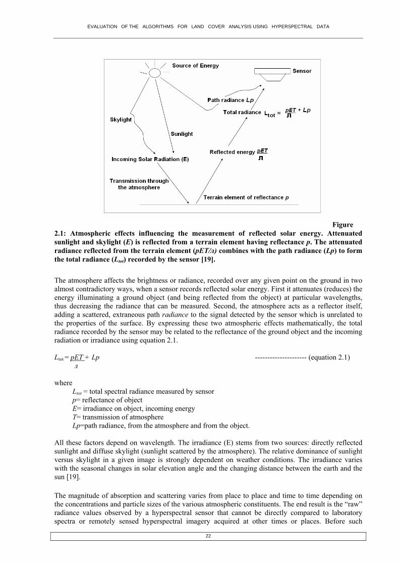
Figure 2.1: Atmospheric effects influencing the measurement of reflected solar energy. Attenuated sunlight and skylight (E) is reflected from a terrain element having reflectance p. The attenuated radiance reflected from the terrain element (pET/л) combines with the path radiance (Lp) to form the total radiance (Ltot) recorded by the sensor [19].
The atmosphere affects the brightness or radiance, recorded over any given point on the ground in two almost contradictory ways, when a sensor records reflected solar energy. First it attenuates (reduces) the energy illuminating a ground object (and being reflected from the object) at particular wavelengths, thus decreasing the radiance that can be measured. Second, the atmosphere acts as a reflector itself, adding a scattered, extraneous path radiance to the signal detected by the sensor which is unrelated to the properties of the surface. By expressing these two atmospheric effects mathematically, the total radiance recorded by the sensor may be related to the reflectance of the ground object and the incoming radiation or irradiance using equation 2.1. Ltot = pET + Lp --------------------- (equation 2.1) л where
Ltot = total spectral radiance measured by sensor p= reflectance of object E= irradiance on object, incoming energy T= transmission of atmosphere Lp=path radiance, from the atmosphere and from the object.
All these factors depend on wavelength. The irradiance (E) stems from two sources: directly reflected sunlight and diffuse skylight (sunlight scattered by the atmosphere). The relative dominance of sunlight versus skylight in a given image is strongly dependent on weather conditions. The irradiance varies with the seasonal changes in solar elevation angle and the changing distance between the earth and the sun [19]. The magnitude of absorption and scattering varies from place to place and time to time depending on the concentrations and particle sizes of the various atmospheric constituents. The end result is the “raw” radiance values observed by a hyperspectral sensor that cannot be directly compared to laboratory spectra or remotely sensed hyperspectral imagery acquired at other times or places. Before such
22

EVALUATION OF THE ALGORITHMS FOR LAND COVER ANALYSIS USING HYPERSPECTRAL DATA
comparisons can be performed, an atmospheric correction process must be used to compensate for the transient effects of atmospheric absorption and scattering. These effects have not been particularly important in the processing and analysis of the multispectral data because of the absence of well defined atmospheric features and the use of average irradiance over each of the recorded wavelengths [45]. Hyperspectral data contain substantial amount of information about atmospheric characteristics at the time of image acquisition. In some cases, atmospheric models can be used with the image data themselves to compute quantities such as the total atmospheric column water vapour content and other atmospheric correction parameters. Alternatively, ground measurements of atmospheric transmittance or optical depth, obtained by instrument such as sunphotometers, may also be incorporated into the atmospheric correction methods. Since hyperspectral data cover a whole spectral range from 0.4 to 2.4 µm, including water absorption features, and have high spectral resolution, a more systematic process is generally required, consisting of three possible steps: 1. Compensation for the shape of the solar spectrum. The measured radiances are divided by solar
irradiances above the atmosphere to obtain the apparent reflectances of the surface. 2. Compensation for atmospheric gaseous transmittances and molecular and aerosol scattering.
Simulating these atmospheric effects allows the apparent reflectances to be converted to scaled surface reflectances.
3. Scaled surface reflectances are converted to real surface reflectances after consideration if any topographic effects. If topographic data are not available, real reflectance is assumed to be identical to scaled reflectance under the assumption that the surfaces of interest are Lambertian.
Procedures for solar curve and atmospheric modelling are incorporated in a number of models [46], including Lowtran 7 (Low Resolution Atmospheric Radiance and Transmittance), 5S Code (Simulation of the Satellite Signal in the Solar Spectrum) and Modtran 3 (The Moderate Resolution Atmospheric Radiance and Transmittance Model) [47]. ATREM (Atmosphere REMoval Program) [48], which is built upon 5S code, overcomes a difficulty with the other approaches in removing water vapour absorption features; water vapour effects vary from pixel to pixel and from time to time. In ATREM the amount of water vapour on a pixel by pixel basis is derived from AVIRIS data itself (although its technique may be independent of type of data), particularly from the 0.94 µm to 1.14 µm water vapour features. A technique referred to as three-channel ratioing was developed for this purpose [46]. Other models like ACORN (Atmospheric CORrection Now) account for accurate and proper cross-track spectral variation of push broom hyperspectral sensor (Hyperion, etc.). It also performs atmospheric correction of multispectral data with an independent water vapour image. FLAASH (Fast Line-of-Sight Atmospheric Analysis of Spectral Hypercubes) is an algorithm that handles data from a variety of hyperspectral sensors including AVIRIS, Hyperion, HyMap, etc., and supports off-nadir as well as nadir viewing. It also includes water vapour and aerosol retrieval and adjacency effect correction. The atmospheric correction algorithm over land (the ACA, Atmospheric Correction Algorithm: Spectral Reflectances for MODIS [49]) are applied to bands 1 – 7 of the MODIS data that uses aerosol and water vapour information derived from MODIS itself and takes into account the directional properties of the observed surface. The data being used in this research are therefore atmospherically corrected. The correction scheme includes corrections for the effects of atmospheric gases, aerosols, and thin cirrus clouds and is applied to all non cloudy L1B pixels that pass the L1B quality. Figure 2.2 gives an overview of the overall methodology and processing for atmospheric corrections [49]. For more relevant information on atmospheric correction see Annexure A.
23

EVALUATION OF THE ALGORITHMS FOR LAND COVER ANALYSIS USING HYPERSPECTRAL DATA
Figure 2.2: Atmospheric correction processing thread flow chart [49].
2.1.3. Radiometric Correction
The radiance measured by any given system over a given object is influenced by such factors as changes in scene illumination, atmospheric conditions, viewing geometry, and instrument response characteristics. For generating mosaics of satellite images taken in visible and NIR portion of the EM, it is usually necessary to apply a sun elevation correction and earth-sun-distance correction. The sun elevation correction accounts for the seasonal position of the sun relative to the earth. This is done by dividing each pixel value in a scene by the sine of the solar elevation angle for the particular time and location of the imaging. It normalises the image data acquired under different solar illumination angles by calculating pixel brightness values assuming the sun was at the zenith on each date of sensing. The earth-sun distance correction is applied to normalise for the seasonal changes in the distance between the earth and the sun. Empirical Line procedure is one of the approaches of radiometric correction [50]. At least two spectrally uniform targets in the site of interest, one dark and one bright, are selected; their actual reflectances are then determined by field or laboratory measurements. The radiance spectra for each target are extracted from the image and then mapped to the actual reflectances using linear regression techniques. The gain and offset so-derived for each band are then applied to all pixels in the image to
24

EVALUATION OF THE ALGORITHMS FOR LAND COVER ANALYSIS USING HYPERSPECTRAL DATA
calculate their reflectances. While computational load is manageable with this method, field or laboratory data may not be available. Another radiometric data processing activity in many quantitative applications is conversion of DNs to absolute radiance values. Such conversions are necessary when changes in the absolute reflectance of objects are to be measured over time using different sensors. Normally, detectors and data systems are designed to produce a linear response to incident spectral radiance. The absolute spectral radiance output of the calibration sources is known from prelaunch calibration and is assumed to be stable over the life of the sensor. Thus the onboard calibration sources form the basis for constructing the radiometric response function by relating known radiance values incident on the detectors to the resulting DNs. The MODIS data being used in the research are radiometrically corrected and fully calibrated at the original instrument spatial and temporal resolution. These data are generated from Level-0 by appending geolocation and calibration data to the raw instrument data. The standard IRS 1C/1D LISS-3 MSS data procured from NRSA (National Remote Sensing Agency), Hyderabad is radiometrically and geometrically corrected. Normally all full scene, full scene Shift Along Track (SAT), sub-scenes and quadrant data products are supplied as standard data products [51].
2.1.4. Data Normalisation
There is special concern about atmospheric spectral transmittance and absorption characteristic and sensor calibration for hyperspectral imagery. This may be due to the following reasons: 1. Hyperspectral sensors bands coinciding with narrow atmospheric absorption features or the edges
of broader spectral features are affected by the atmosphere differently than the neighbouring bands.
2. The band locations in imaging spectrometer systems are prone to small wavelength shifts under different operating conditions, particularly in airborne sensors.
A number of empirical techniques have been developed for the calibration of hyperspectral data that produce relative or absolute calibrations in an empirical way, without the explicit use of atmospheric data and models; for the reason they are more properly referred to as normalisation techniques, rather than calibration techniques. When detailed radiometric correction is not feasible (for example, because the necessary ancillary information is unavailable) normalisation is an alternative which makes the corrected data independent of multiplicative noise such as topographic and solar spectrum effects. This can be performed using Log Residuals [52], based on the relationship between radiance (raw data) and reflectance: Xi, n = TiRinIn, i = 1,…K; n = 1,…..N ------------------- (equation 2.2)
where Xi, n is radiance for pixel i in wavelength n. Ti is the topographic effect, which is assumed constant for all wavelengths. Rin is the real reflectance for pixel i in wavelength band n. In is the (unknown) illumination factor, which is assumed independent of pixel. K and N are the total number of the pixels in the image and the total number of bands, respectively. There are two steps which remove the topographic and illumination effects respectively. Xi, n can be made independent of Ti and In by dividing Xi,n by its geometric mean over all bands and then its geometric mean over all pixels. The result is not identical to reflectance but is independent of the multiplicative illumination and topographic effects present in the raw data. The procedure is carried out logarithmically so that the geometric means are replaced by arithmetic means and the final result obtained for the normalised data is N K Log Zi, n = log Xi, n – log mn – log mi = log Xin – 1/N ∑ log Xi, n – 1/K ∑ log Xi, n -----(equation 2.3) n=1 i=1
25

EVALUATION OF THE ALGORITHMS FOR LAND COVER ANALYSIS USING HYPERSPECTRAL DATA
2.2. Data Characteristics
The data produced by the imaging spectrometers is different from that of multispectral instruments due to its spectral characteristics. Firstly, the band selection for the display device is done in such a way so as to display maximum information. A two dimensional display using one geographical dimension and the spectral dimension can be created. These types of representation allows changes in spectral signatures with position (either along track or across track) to be observed. Usually, the greyscale is mapped to colour to enhance the interpretability of the displayed data. Secondly, choosing the most appropriate channels for processing is also not straight forward and requires careful selection to minimise the loss of the spectral benefits offered by this form of data gathering. A simple linear transformation such as the Principal Component Analysis or the Minimum Noise Fraction can be used for data dimensionality reduction [45].
2.2.1. Data Volume
Although, the hyperspectral data are both voluminous and multidimensional, nowadays with the availability of advanced computing systems that possess high speed processors and enormous storage power, data volume is no longer a constraint. The problem lies in the data redundancy that needs to be removed to obtain the bands with maximum information.
2.2.2. Redundancy
Much of the data does not add to the inherent information content for a particular application, even though it often helps in discovering that information; it contains redundancies. The data recorded by hyperspectral sensors often have substantial overlap of information content over the bands of data recorded for a given pixel. In such cases, not all of the data are needed to characterise a pixel properly, although redundant data may be different for different applications. Data redundancy can take two forms; spatial and spectral. Since hyperspectral imagery has more spectral concern, one way of viewing spectral redundancy in hyperspectral data is to form the correlation matrix for an image; the correlation matrix can be derived from the covariance matrix. High correlation between band pairs indicates high degree of redundancy. For example, PCT (Principal Component Transformation) assist in removing redundancy since decorrelation followed by a discarding of low variance components amounts to redundancy reduction [45].
2.3. Feature reduction / Band reduction / Data dimensionality reduction techniques
Removal of least effective feature is referred to as feature selection, this being one form of feature reduction. The other is to transform the pixel vector into a new set of co-ordinates in which the features that can be removed are more evident [45]. Therefore, feature reduction, i.e., band reduction, has become a more significant part of image interpretation process. Probably the most common approach is to employ some sort of linear transformation on the original dataset to produce a smaller set of factors or components [53], [54] and [55]. Most of the original variance is retained with a significant reduction in data volume [1].
2.3.1. Principal Component Analysis (PCA)
PCA transform multidimensional image data into a new, uncorrelated co-ordinate system or vector space. It produces a space in which the data have maximum variance along its first axis, the next largest variance along a second mutually orthogonal axis and so on (figure 2.3). Sometimes even the lower-order PC’s may contain valuable information. The later principal components would be expected, in general, to show little variance. These could be considered therefore to contribute little to separability and could be ignored, thereby reducing the essential dimensionality of the classification space and thus improving classification speed [45]. Stated differently, the purpose of this process is to compress all the information contained in an original n – band data set into fewer than n “new bands” or components. The components are then used in lieu of the original data [19]. These transformations may be applied as
26

EVALUATION OF THE ALGORITHMS FOR LAND COVER ANALYSIS USING HYPERSPECTRAL DATA
a preprocessing procedure prior to automated classification process of the data. Fundamentals and mathematical description of PCA are given in Annexure A.
Figure 2.3: Rotated coordinate axes in PCA [19].
2.3.2. Minimum Noise Fraction (MNF)
covariance matrix, is to decorrelate and rescale the data noise, where the
ments for subsequent processing. It partitions the data space into o parts: one associated with large eigenvalues and coherent eigenimages, and a second with near-
nity eigenvalues and noise-dominated images. By using only the coherent portions in subsequent rocessing, the noise is separated from the data, thus improving spectral processing results [58].
his transformation is equivalent to principal components when the noise variance is the same in all ands [56]. By applying the MNF to the Geophysical and Environment Research (GER) 64-band data, e results demonstrated the effectiveness of this transformation for noise adjustment in both the spatial
nd spectral domains [59]. Although PCA can efficiently compress hyperspectral data into a few components, this high concentration of total covariance only in the first few components inevitably results from part of the
component lysis. MNF,
This transformation is mainly used to reduce the dimensionality of hyperspectral data before performing the data fusion. It was first developed as an alternative to PCA for the airborne Thematic Mapper (ATM) 10- band sensor [56]. It is defined as a two-step cascaded PCA [57]. The first step,
ased on an estimated noisebnoise has unit variance and no band-to-band correlations. The next step is a standard PCA of the noise-whitened data. The MNF transformation is a linear transformation related to PC that orders the data according to signal-to-noise-ratio. It determines the inherent dimensionality of the data, segregates noise in the data nd reduces the computational requirea
twup Tbtha
noise variance [56], [59] and [60]. The special capability image quality with increasingnumber cannot be accomplished easily using other techniques, such as PCA and factor anahowever, can help in this regard [61].
27

EVALUATION OF THE ALGORITHMS FOR LAND COVER ANALYSIS USING HYPERSPECTRAL DATA
3. Hard Classification Techniques
Land cover analysis is the first level of classification that helps in identifying land cover in terms of vegetation and non vegetation. This is done by slope based and distance based indices depending on the region (arid versus vegetated area). The slope based and the distance based vegetation indices (VIs)
elp in land cover analysis depending on the extent h of vegetation and soil in a region. The slope-based
rties. The term pattern refers to the set of radiance bands for each pixel. Spectral pattern recognition
ed for land cover
its background soil brightness and
VIs are simple arithmetic combinations that focus on the contrast between the spectral response patterns of vegetation in the red and near-infrared portions of the electromagnetic spectrum. The distance-based group measures the degree of vegetation present by gauging the difference of any pixel’s reflectance from the reflectance of bare soil. Different feature types lead to different combinations of DNs (Digital Numbers) based on their inherent spectral reflectance and emittance propemeasurements obtained in the various wavelength refers to the family of classification procedures that utilizes this pixel-by-pixel spectral information as the basis for automated image classification and, indeed, the spectral pattern present within the data for each pixel is used as the numerical basis for categorization [19]. The overall objective of image classification procedures is to automatically categorise all pixels in an image into land cover classes or themes. Spectral Classification can be broadly categorised in to two types: Supervised classification and Unsupervised Classification. This chapter discusses the most commonly used Vegetation Index; NDVI (Normalized Difference Vegetation Index) for land cover mapping, and then highlights the various hard classification techniques including Supervised and Unsupervised (K-means algorithm) that are usmapping. A comparison of the advantages and the disadvantages of the supervised and unsupervised approach is summarised and the chapter concludes with a brief discussion on the accuracy assessment.
3.1. NDVI time series analysis
Vegetated areas have a relatively high near-IR (Infrared) reflectance and low visible reflectance. Due to this property of the vegetation, various mathematical combinations of the NIR and the Red band have been found to be sensitive indicators of the presence and condition of green vegetation. These mathematical quantities are thus referred to as vegetation indices [19]. The most commonly used of these indices is the NDVI (Normalized Difference Vegetation Index) that is computed using the
rmula (NIR-RED)/(NIR+RED). It separates green vegetation fromforetains the ability to minimize topographic effects while producing a measurement scale ranging from –1 to +1 with NDVI-values ≤ 0 representing no vegetation. The NDVI is sensitive to the presence of vegetation, since green vegetation usually decreases the signal in the red due to chlorophyll absorption and increases the signal in the NIR wavelength due to light scattering by leaves [62]. The success of the NDVI to monitor vegetation variations on a large scale, despite the presence of atmospheric effects [63], [64] and [65] is due to the normalisation involved in its definition. The normalization reduces the effect of degradation of the satellite calibration from 10% - 30% for a single hannel to 0-6% for the normalized index [66] and [67]. The effect of the angular dependence of the c
surface bidirectional reflectance and of the atmospheric effects is also reduced significantly in the normalized index [66], [69] and [70]. The effect of scattering and absorption by atmospheric aerosol and gases (mainly water vapour) and by undetected clouds is reduced significantly in the compositing of the NDVI from several consecutive images, choosing a value that corresponds to the maximum vegetation index for each pixel [69], [70] and [71].
28
EVALUATION OF THE ALGORITHMS FOR LAND COVER ANALYSIS USING HYPERSPECTRAL DATA
The potential of computing NDVI has created great interest to study global biosphere dynamics [72]. It is preferred to the simple index for global vegetation monitoring because the NDVI helps compensate for changing illumination conditions, surface slope, aspect and other extraneous factors. Numerous investigators have related the NDVI to several vegetation phenomena. These phenomena have ranged from vegetation seasonal dynamics at global and continental scales, to tropical forest clearance, leaf area index measurement, biomass estimation, percentage ground cover determination and FPAR (fraction of absorbed photosynthetically active radiation). In turn, these vegetation attributes are used in various models to study photosynthesis, carbon budgets, water balance and related processes [19]. Many researchers have attempted to produce regional-scale land cover datasets using coarse spatial-
ues due to differential scattering effects in red and near-infrared ands. Cloud-contaminated measurements also produce lower NDVI values, as clouds reflect strongly
, [77]) have found that using a time series of the ratio of surface mperature to NDVI provides a more stable classification than NDVI alone, primarily by isolating
ity of the NDVI. Lloyd [80] employed a binary lassifier based on summary indices derived from a time series of NDVI data. These phytophenological
resolution, high temporal-frequency data from the AVHRR instrument aboard the NOAA series of meteorological satellites. Almost without exception, these efforts have involved the conversion of AVHRR bands 1 and 2 to Normalised Difference Vegetation Index (NDVI) values. A registered time series of NDVI images is then composited so that, for every pixel location, the maximum NDVI value encountered throughout the compositing period is output. The compositing procedure tends to select against measurements that are strongly influenced by atmospheric and aerosol scattering. These measurements have reduced NDVI valbin both the red and near-infrared wave bands. The compositing of NDVI values further reduces the variability associated with changing view and illumination geometry [68], although measurements near the forward-scattering direction tend to have slightly higher NDVI values and will thus be preferentially selected. Compositing periods are chosen based on a trade-off between the expected frequency of changes in vegetation and the minimum length of time necessary to produce cloud-free images. NDVI generally quantifies the biophysical activity of the land surface and, as such, does not provide land cover type directly. However, a time series of NDVI values can separate different land cover types based on their phenology, or seasonal signals (e.g. [73]). Reed et al. [74] and DeFries et al. [75] have developed and used multitemporal phenological metrics to derive land cover classifications from AVHRR data. Lambin and Ehrlich ([76]teinterannual climatological variability. Townshend [78] performed supervised classifications on composited NDVI GAC (Global Area Coverage) data for South America. While they did not validate their results with test data, they found that accuracy for the training sites improved substantially with the increase in the number of images included in the time series. Koomanoff [79] used annually-integrated NDVI values to generate a global vegetation map using NOAA’s Global Vegetation Index product (GVI). This work represents nine vegetation types and does not rely on the seasonalcvariables included the date of the maximum photosynthetic activity, the length of the growing season, and the mean daily NDVI value. The variables were fed through a binary decision tree classifier that stratified pixels based first on the date of the maximum NDVI, then the length of the growing season, and finally on the mean daily NDVI. A coarse-resolution global land surface parameter database was generated as an activity of the International Satellite Land Surface Climatology Project (ISCLSCP) [81]. The database includes land cover classes, absorbed fraction of photosynthetically-active radiation (FPAR), leaf area index (LAI), roughness length, and canopy greenness fraction, along with data on global meteorology, soils and hydrology. The spatial scale of the database is 1 degree by 1 degree. Variables such as FPAR, LAI and canopy greenness fraction are derived from 8-km composited AVHRR NDVI data. The land cover classification is based on a spatial aggregation of the 8-km data to one degree followed by supervised classification of the temporal patterns in NDVI [18].
29

EVALUATION OF THE ALGORITHMS FOR LAND COVER ANALYSIS USING HYPERSPECTRAL DATA
Loveland’s efforts were expanded under the auspices of the IGBP-DIS (International Geosphere Biosphere Programme-Data and Information System), based on a global database of 1-km AVHRR observations received during the period April 1992 through September 1993 [82] and [83]. These have been assembled and 10-day composited at the EROS Data Center (EDC). The 10-day composite AVHRR data were then monthly composited using maximum NDVI to remove cloud and topographic
, as well as scan angle dependence of radiance [85].
projectito the Gooconfusegeneral The glo
.2. Supervised Classification
rvised c y specifying the numerical
he following subsections discuss the classification strategies that use the ‘training set’ descriptions of
um likelihood classifier quantitatively evaluates both the variance and covariance of the category spectral response patterns when classifying an unknown pixel. It is assumed that the distribution of the cloud of points forming the category training data is Gaussian (normally distributed). This assumption of normality is generally reasonable for common spectral response distributions. Under this assumption, the distribution of a category response pattern can be completely described by the mean vector and the covariance matrix. With these parameters, the statistical probability of a given pixel value being a member of a particular land cover class can be computed. The resulting bell-shaped surfaces are called probability functions, and there is one such function for each spectral category [19]. The probability density functions are used to classify an unidentified pixel by computing the probability of the pixel value belonging to each category. After evaluating the probability in each category, the pixel is assigned to the most likely class (highest probability value) or can be labelled as “unknown” if the probability values are all below a threshold set by the analyst. Essentially, the maximum likelihood classifier delineates ellipsoidal “equiprobability contours” through a scatter diagram as shown in figure 3.1 [19].
effects and extreme off-nadir pixels [68] and [84]The use of the monthly-composited AVHRR data may be problematic [68]. An analysis by Zhu and Yang [86] determined that compositing was biased towards selecting off-nadir pixels, especially in forward-scanning views in winter months in the northern hemisphere. As with any large-area
on, they also found that the effective mapping unit was geographically variable, in this case due de’s homolosine projection system and resampling methods. Lack of sensor calibration
s the temporal trajectory of the multitemporal NDVI signal [87]. Temporal smoothing or ization might enhance the meaning of the temporal signal [98].
al NDVI data provided a multitemporal database for land cover classification using anbunsupervised clustering and labeling approach. The global IGBP product has recently undergone validation based on a global network of some 400 stratified samples that were characterized using finer-resolution Landsat TM and SPOT-XS data following an expert interpretation approach [1].
3
In supe lassification, the pixel categorization process is done bdescriptors of the various land cover types present in a scene. It involves three steps –
(1) training stage: identifying representative training areas and developing a numerical description of the spectral attributes of each land cover type in the scene, known as training set,
(2) classification stage: each pixel in the image data set is categorized into the land cover class it most closely resembles, and
(3) output stage: the process consists of a matrix of interpreted land cover category types [19].
Tthe category spectral response patterns as interpretation keys by which pixels of unidentified cover type are categorised into their appropriate classes.
3.2.1. Gaussian Maximum Likelihood Classifier (GMLC)
The maxim
30

EVALUATION OF THE ALGORITHMS FOR LAND COVER ANALYSIS USING HYPERSPECTRAL DATA
Figure 3.1: Equiprobability contours defined by a maximum-likelihood classifier.
An extension of the maximum likelihood approach is the Bayesian classifier. This technique applies two weighting factors to the probability estimate. First, the “a priori probability”, or the anticipated likelihood of occurrence for each class in the given scene is determined. Secondly, a weight associated with the “cost” of misclassification is applied to each class. Together, these factors act to minimize the “cost” of misclassification, resulting in a theoretically optimum classification. Most maximum likelihood classifications are performed assuming equal probability of occurrence and cost of misclassification for all classes. If suitable data exist for these factors, the Bayesian implementation of the classifier is preferable [19]. For a mathematical description of Bayes’ Classification see Annexure B.
3.2.1.1. Drawback of the GMLC Technique
The successful application of MLC is dependent upon having delineated correctly the spectral classes in the image data of interest. This is necessary since each class is to be modelled by a normal probability distribution, as discussed earlier. If a class happens to be multimodal, and this is not resolved, then clearly the modelling cannot be very effective [45]. The drawback of maximum likelihood classification is the large number of computation required to classify each pixel. This is particularly true when either a large number of spectral channels are involved or a large number of spectral classes must be differentiated. In such cases, the maximum likelihood classifier is much slower computationally than other algorithms [19]. In addition, MLC requires that every training set must include at least one more pixel than there are bands in the sensor and more often it is desirable to have the number of pixels per training set be between 10 times and 100 times as large as the number of sensor bands, in order to reliably derive class-specific covariance matrices. To increase the efficiency, of the maximum likelihood classifiers, the category identity for all possible combinations of digital numbers occurring in an image is determined in advance of actually classifying the image. Hence, the complex statistical computation for each combination is only made once. The categorization of each pixel in the image is then simply a matter of indexing the location of its
31

EVALUATION OF THE ALGORITHMS FOR LAND COVER ANALYSIS USING HYPERSPECTRAL DATA
multichannel gray level. Another means of optimizing the implementation of the MLC is to use some data dimensionality reduction technique [19].
3.2.2. Spectral Angle Mapper (SAM)
In N dimensional multi-(or hyper-) spectral space a pixel vector x has both magnitude (length) and an angle measured with respect to the axes that defines the coordinate system of the space [45]. In the Spectral Angle Mapper (SAM) technique for identifying pixel spectra only the angular information is used. SAM is based on the idea that an observed reflectance spectrum can be considered as a vector in a multidimensional space, where the number of dimensions equals the number of spectral bands. If the overall illumination increases or decreases (due to the presence of a mix of sunlight and shadows), the length of this vector will increase or decrease, but its angular orientation will remain constant. Figure 3.2 (a) shows that for a given feature type, the vector corresponding to its spectrum will lie along a line passing through the origin, with the magnitude of the vector being smaller (A) or larger (B) under lower or higher illumination, respectively. Figure 3.2 (b) shows the comparison of the vector for an unknown feature type (C) to a known material with laboratory-measured spectral vector (D), the two features match if the angle ‘α’ is smaller than a specified tolerance value [89].
Figure 3.2: Spectral Angle Mapping concept. (a) For a given feature type, the vector corresponding to its spectrum will lie along a line passing through the origin, with the magnitude of the vector being smaller (A) or larger (B) under lower or higher illumination, respectively. (b)
hen comparing the vector for an unknown feature type (C) to a known material with
e defined for each spectrum and the angle between the two vectors is calculated. Smaller angles represent closer matches to the reference spectrum. If this angle is smaller
spectra are considered to match, even if one spectrum is much brighter
medium spatial resolution sensors, such as Quickbird and
Wlaboratory-measured spectral vector (D), the two features match if the angle ‘α’ is smaller than a specified tolerance value. (After Kruse et al., 1993) [34].
To compare two spectra, such as an image pixel spectrum and a library reference spectrum, the multidimensional vectors ar
than a given tolerance level, thethan the other (farther from the origin) overall [19]. Pixels further away than the specified maximum angle threshold are not classified. The reference endmember spectra used by SAM can come from ASCII files, spectral libraries, statistics files, or can be extracted directly from the image. Girouard et al. [90] validated the SAM algorithm for geological mapping in Central Jebilet Morocco and compared the results between high and Landsat TM, respectively. The result showed that SAM of TM data can provide mineralogical maps that compare favourably with ground truth and known surface geology maps. Even though, Quickbird has a high spatial resolution compared to TM; its data did not provide good results for SAM because of the low spectral resolution.
32

EVALUATION OF THE ALGORITHMS FOR LAND COVER ANALYSIS USING HYPERSPECTRAL DATA
3.2.2.1. Drawback of SAM
SAM technique fails if the vector magnitude is important in providing discriminating information, which happens in many instances [45]. However, if the pixel spectra from the different classes are well distributed in feature space there is a high likelihood that angular information alone will provide good
aration. This technique functions well in the face of scaling noisesep .
process. In addition, once they have been fully trained, neural
ore hidden layers.
bility to generalize, and increases the time required for training [19].
igure 3.3 shows an example of a neural network that is used to classify land covers based on a bination of spectral information. There are seven nodes in the input layer (Spectral Bands 1 to 7).
After the input layer, there are two hidden layers, each with nine nodes. Finally, the output layer consists of six nodes, each corresponding to a land cover class. When given any combination of input data, the network produces the output class that is most likely to result from that set of inputs, based on the network’s analysis of previously supplied data. Applying a NN to image classification makes use of an iterative training procedure in which the network is provided with matching sets of input and output data. Each set of input data represents an example of a pattern to be learned, and each corresponding set of output data represents the desired output that should be produced in response to the input. During the training process the network autonomously modifies the weights on the linkages between each pair of nodes in such a way as to reduce the discrepancy between the desired output and the actual output [19].
3.2.3. Neural Network
To overcome difficulties in conventional digital classification that uses the spectral characteristics of the pixel as the sole parameter in deciding to which class a pixel belongs to, new approaches such as Neural Networks (NN) are being used. They can be used to perform traditional image classification tasks [91] and are also increasingly used for more complex operations such as spectral mixture analysis [92]. For image classification, neural networks do not require that the training class data have a Gaussian statistical distribution, a requirement that is held by maximum-likelihood algorithms. This allows neural networks to be used with a much wider range of types of input data than could be used in a traditional
aximum-likelihood classification mnetworks can perform image classification relatively rapidly, although the training process itself can be quite time consuming. NN systems are “self-training” in that they adaptively construct linkages between a given pattern of input data and particular outputs [19]. A NN consists of a set of three or more layers, each made up of multiple nodes. These nodes are somewhat analogous to the neurons in a biological neural network and thus are sometimes referred to as neurons”. The network’s layers include an input layer, an output layer, and one or m“
The nodes in the input layer represent variables used as input to the neural network. Typically, these might include spectral bands from a remotely sensed image, textural features or other intermediate products derived from such images, or ancillary data describing the region to be analysed. The nodes in the output layer represent the range of possible output categories to be produced by the network. If the network is being used for image classification, there will be one output node for each class in the classification system [19]. Between the input and output layers are one or more hidden layers. These consist of multiple nodes, each linked to many nodes in the preceding layer and to many nodes in the following layer. These linkages between nodes are represented by weights, which guide the flow of information through the network. The number of hidden layers used in a neural network is arbitrary. An increase in the number
f hidden layers permits the network to be used for more complex problems but reduces the network’s oa Fcom
33

EVALUATION OF THE ALGORITHMS FOR LAND COVER ANALYSIS USING HYPERSPECTRAL DATA
Figure 3.3: Example of an artificial neural network with one input layer, two hidden layers and one output layer [19].
The bulk of neural network classification work in remote sensing has used multiple layer feed-forward networks that are trained using the back-propagation algorithm based on a recursive learning procedure with a gradient descent search [4]. However, this training procedure is sensitive to the choice of initial network parameters and to over-fitting [93]. The use of Adaptive Resonance Theory (ART) can overcome these problems. Networks organized on the ART principle are stable as learning proceeds, while at the same time they are flexible enough to learn new patterns and improves especially the overall accuracy of classification of multi-temporal data sets [94], [93]. Recent MODIS-based land cover classification used a class of ART NN called fuzzy ARTMAP, for classification, change detection and mixture modelling. Many studies based on ARTMAP have been directed toward recognition of land cover classes, which have ranged from broad life-form categories [95] to floristic classes [96]. Remotely sensed datasets processed by NN-based classifiers have included images acquired by the Landsat Multispectral Scanner (MSS) [97], [98], Landsat TM [99], Synthetic Aperture Radar [100], SPOT HRV [101], AVHRR [94] and aircraft scanner data [102]. A number of these studies have also included ancillary data e.g., topography [103] and texture [104]. Most use a supervised approach, but unsupervised classification using self-organizing neural networks has also been attempted [100]. In all cases, the neural network classifiers have proven superior to conventional classifiers, often recording overall accuracy improvements in the range of 10-20 percent. As the number of successful applications of neural network classification increases, it is increasingly clear that neural network-based classification can produce more accurate results than conventional approaches for remote sensing.
3.2.3.1. Summary of Neural Network
While there are a variety of different NN models, most remote sensing applications have used a supervised, feedforward structure employing a backpropagation algorithm that adjusts the network weights to produce convergence between the network outputs and the training data. In overview, the
34

EVALUATION OF THE ALGORITHMS FOR LAND COVER ANALYSIS USING HYPERSPECTRAL DATA
NN classifier is composed of layers of “neurons” that are interconnected through weighted synapses. The first layer consists of the classification input variables and the last layer consists of a binary vector representing the output classes. Intermediate, “hidden” layers provide an internal representation of neural pathways through which input data are processed to arrive at output values or conclusions. In a supervised approach, the neural network is trained on a dataset for which the output classes are known. In this process, the input variables are fed forward through the network to produce an output vector. During a following backpropagation phase, the synapse weights are adjusted so that the network output vector more closely matches the desired output vector, which is a binary-coded representation of the training class. The network weights, or processing element responses, are adjusted by feeding the summed squared errors from the output layer back through the hidden layers to the input layer. In this fashion, the network cycles through the training set until the synapse weights have been adjusted so that the network output has converged, to an acceptable level, with the desired output. The trained neural network is then given new data, and the internal synapses guide the processing flow through excitement and inhibition of neurons. This results in the assignment of the input data to the output classes.
3.2.3.2. Advantages and drawbacks of Neural Networks
(i) Neural network classifiers, without any priori assumptions about data distributions, are able to learn nonlinear and discontinuous patterns in the distribution of classes.
(ii) Neural networks can readily accommodate auxiliary data such as textural information, slope, aspect and elevation, and
(iii) Neural networks are quite flexible and can be adapted to improve performance for particular problems [1].
The back propagation NN is not guaranteed to find the ideal solution to a particular problem. During the training process the network may develop in such a way that it becomes caught in a “local minimum” in the output error field, rather than reaching the absolute minimum error. Alternatively, the network may begin to oscillate between two slightly different states, each of which results in approximately equal error [105]. A variety of strategies have been proposed to help push neural networks out of these pitfalls and enable them to continue development toward the absolute minimum error. Again, the use of ANN in image classification is the subject of continuing research [19].
3.2.4. Decision Tree Approach
Decision tree approach is a non-parametric classifier and an example of machine learning algorithm. It involves a recursive partitioning of the feature space, based on a set of rules that are learned by an analysis of the training set. A tree structure is developed where at each branching a specific decision rule is implemented, which may involve one or more combinations of the attribute inputs. A new input vector then “travels” from the root node down through successive branches until it is placed in a specific class [4]. The thresholds used for each class decision are chosen using minimum entropy or minimum error measures. It is based on using the minimum number of bits to describe each decision at a node in the tree based on the frequency of each class at the node. With minimum entropy, the stopping criterion is based on the amount of information gained by a rule (the gain ratio) [4]. A decision tree is composed of a root node, a set of interior nodes, and terminal nodes, called “leaves”. The root node and interior nodes, referred to collectively as non-terminal nodes, are linked into decision stages. The terminal nodes represent final classification. The classification process is implemented by a set of rules that determine the path to be followed, starting from the root node and ending at one terminal node, which represents the label for the object being classified. At each non-terminal node, a decision has to be taken about the path to the next node. Figure 3.4 illustrates a simple decision tree using pixel reflectance as input [4].
35

EVALUATION OF THE ALGORITHMS FOR LAND COVER ANALYSIS USING HYPERSPECTRAL DATA
Figure 3.4: Example of Decision Tree
• If there are k classes denoted {C1, C2,….Ck}, and a training set, T, then • If T contains one or more objects which all belong to a single class Cj, then the decision tree is
pt was m s under different manure/fertilizer
tree algorithm of data mining technology was used to ments. The decision tree approach divided the
any tree branches.
e study suggest that the decision tree lassifier performs well. The boosting technique improved the classification accuracy of a base
a leaf identifying class Cj. • If T contains no objects, the decision tree is a leaf determined from information other than T. • If T contains objects that belong to a mixture of classes, then a test is chosen, based on a single
attribute that has one or more mutually exclusive outcomes {O1, O2,…On}. T is portioned into subsets T1, T2,…Tn, where Ti contains all the objects in T that have outcome Oi of the chosen test. The same method is applied recursively to each subset of training objects to build the decision tree.
An attem ade by [106] to classify the agricultural fieldapplication strategies. During the summer of 2000, airborn hyperspectral data were collected three times at two field sites in south-western Quebec, Canada. One field site contained plots that were amended with manure treatments and planned with maize and soya beans. The second field site contained plots that received chemical fertilizers and were planted with maize. Reflectances of 71 wave bands of hyperspectral data were collected and the decision distinguish between manure and chemical fertilizer treatdata to reduce the deviance, and classified them into the pre-defined categories as mThe success of the classification rate was reported to be high. A decision tree classifier was used for land use classification using Landsat-7 ETM+ data for an agricultural area near Littleport (Cambridgeshire), UK, for the year 2000. A field study was carried out to collect ground truth information about the various land use classes. Six land use classes (wheat, sugar beet, potatoes, peas, onions and lettuce) were selected for classification, and a univariate decision tree classifier was used for labelling the image pixels. The results of thcclassifier and the classification accuracy increased [107].
3.2.4.1. Advantages of Decision Tree Approach
The advantages of decision tree classifier over traditional statistical classifier include its simplicity, ability to handle missing and noisy data, and non-parametric nature. Decision trees are not constrained
36

EVALUATION OF THE ALGORITHMS FOR LAND COVER ANALYSIS USING HYPERSPECTRAL DATA
by any lack of knowledge of the class distributions. It can be trained quickly, takes less computational time.
3.3. Unsupervised Classification
The strength of supervised classification based upon the maximum likelihood procedure is that it minimises classification error for classes that are distributed in a multivariate normal fashion. Moreover, it can label data relatively quickly. Its major drawback lies in the need for training data and the need to have delineated unimodal spectral classes beforehand. This, however, is a task that can be handled using clustering, based upon a representative subset of image data. Used for this task,
on performs the valuable function of identifying the existence of all spectral
spectrally similar pixels has been established in the image data. This
lities of class em
by p
3.3
sers o sses. Occasionally it might be in general, the user
in multispectral pac pplied in
man itions the imathos p…… aclas
terest,
unsupervised classificaticlasses, yet it is not expected to perform the entire classification. Unsupervised Classification is an analytical procedure based upon clustering algorithms. Unsupervised classifiers do not utilize training data as the basis for classification. Rather they examine the unknown pixels in an image and aggregate them into a number of classes based on the natural groupings or clusters present in the image values. The basic premise is that the values within a given cover type should be close together in the measurement space, whereas data in different classes should be comparatively well separated. The classes that result from unsupervised classification are spectral classes. Thus, here spectrally separable classes are determined and then their informational utility is defined [19]. The identification of classes of interest against reference data is often more easily carried
ut when the spatial distribution ofois an advantage of unsupervised classification and the technique is therefore a convenient means by which to generate signatures for spatially elongated classes such as rivers and roads [45]. Consequently, it is not unusual in practice to iterate over sets of steps as experience is gained with the particular problem at hand [45]. A final point that must be taken into account when contemplating unsupervised lassification via clustering is that there is no facility for including prior probabic
m bership. By comparison the decision functions for maximum likelihood classification can be biased revious knowledge or estimates of class membership [45].
.1. Clustering
f remotely sensed data can only specify the information claUpossible to guess the number of spectral classes in a particular information class but,
ould have little idea of the number of distinct unimodal groups that the data falls into ws e. Clustering procedures can be used for that purpose. These are methods that have been a
Clustering party data analysis fields to enable inherent data structures to be determined.dge ata into a number of spectral classes, and then labels all pixels of interest as belonging to one of
e s ectral classes, although the labels are purely nominal (e.g. A, B, C, …., or class1, class 2, .) nd are as yet unrelated to ground cover types. Clustering is also the basis for unsupervised
sification. The classes are preferably unimodal; however, if simple unsupervised classification is of this is not essential [45]. in
Clustering techniques fall into a group of undirected data mining tools [108]. The goal of clustering is to discover structure in the data as a whole. There is no target variable to be predicted and thus no distinction is being made between independent and dependent variables. Clustering techniques are used for combining observed examples into clusters (groups) which satisfy two main criteria:
a) Each group or cluster is homogeneous; i.e. examples that belong to the same group are similar to each other.
b) Each group or cluster should be different from other cluster, i.e. examples that belong to one cluster should be different from the examples of other clusters.
Depending on the clustering technique, clusters can be expressed in different ways:
a) Identified clusters may be exclusive, so that any example belongs to only one cluster.
37

EVALUATION OF THE ALGORITHMS FOR LAND COVER ANALYSIS USING HYPERSPECTRAL DATA
b) They may be overlapping, an example may belong to several clusters.
st employed to determine the spectral classes, using a subset of the image data. It is erefore recommended that about 3 to 6 small regions, or so-called candidate clustering areas, be
an iterative clustering procedure is used, the analyst will have to pre-specify the number of clusters
ring is generated on a sample of data, with a second phase o a cluster. Feature selection would be performed between the two
ecisions about merging can be made on the basis of separability measures. During the rationalisation
ents. Sometimes, depending pon the cases in hand, the most significant pair of spectral bands would be chosen in order to view the
i-
This s r an average, an average location of all the members of a particular cluster). When dealing with
ents a distance of example from the origin along the attribute axes. Of course, in order to use this geometry
c) They may be probabilistic, whereby an example belongs to each cluster with a certain probability.
d) Clusters might have hierarchical structure, having crude division of examples at highest level of hierarchy, which is then refined to sub-clusters at lower levels.
Clustering is firthchosen for this purpose. These should be well spaced over the image and located such that each one contains several of the cover types (information class) of interest and such that all cover types are represented in the collection of clustering areas. An advantage in choosing heterogeneous regions to cluster, as against apparently homogeneous training areas used in supervised classification, is that mixture pixels lying on class boundaries will be identified as legitimate spectral classes [45]. Ifexpected in each candidate area. Experience has shown that, on average, there are about 2 to 3 spectral classes per information class. This number should be chosen with a view of removing or rationalising unnecessary clusters at a later stage. It is useful to cluster each region separately as this saves computation, and produces cluster maps within those areas with more distinct class boundaries than would be the case if all regions were pooled beforehand [45]. Most clustering procedures in remote sensing generate the mean vector and covariance matrix for each cluster found. Accordingly, separability measures can be used to assess whether feature reduction is necessary or whether some clusters are sufficiently similar spectrally and should be merged. These are only considerations of course if the clusteused to allocate all image pixels tphases [45]. Clustering sorts the image into unknown classes [45]. Following this sorting of the data space by clustering, the clusters or spectral classes are associated with information classes – i.e. ground cover types – by the analyst, using available reference data. Thus a posteriori identification may need to be performed explicitly only for classes of interest. The other classes will have been used by the algorithm to ensure good discrimination but will remain labelled only by arbitrary symbols rather than by class names [45]. Dprocedure it is useful to be able to visualise the locations of spectral classes. For this a bispectral plot can be constructed. This bispectral plot is not unlike a two dimensional scatter plot view of the multispectral space in which the data appears. However, rather than having the individual pixels shown, the class or cluster means are located according to their spectral componurelative locations of the cluster centres. In general, the choice of bands and combinations to use in a bspectral plot will depend on the sensor and application. Sometimes, several plots with different bands will give a fuller appreciation of the distribution of classes in feature space [45]. For a discussion on clustering criteria, please see Annexure B.
2. K – Means Algorithm 3.3.
algorithm has as an input, a predefined number of clusters (i.e., the K from its name. Means standfoclustering techniques, one has to adopt a notion of a higher dimensional space, or space in which orthogonal dimensions are all attributes. The value of each attribute of an example repres
the efficiently, the values in the data set must all be numeric (categorical data must be transformed into numeric ones) and should be normalized in order to allow fair computation of the overall distances in a multi-attribute space.
38

EVALUATION OF THE ALGORITHMS FOR LAND COVER ANALYSIS USING HYPERSPECTRAL DATA
The K-means algorithm is a simple, iterative procedure, in which a crucial concept is the one of centroid”. Centroid is an artificial point in the space of records which represents an average location of
this point are averages of attribute values of all examples that to -means algorithm are given below.
ii) Calculate new centroids of the clusters. For that purpose, average all attribute values of the
this ples to clusters needs ee Annexure B.
of the data space in the absence of any information provided by any nalyst. Analyst information is used only to attach information class (or ground cover type, or map)
pared ith clustering. For example, for Landsat MSS data, therefore, in a situation where all 4 spectral bands
are used, clustering would have to be completed within be speed MLC. Trainin lassifie % mand; however a significant time loading should also be added to clustering to acco labelling phase. Often this is done by associating pixels with the nearest (Euclidean dista er, som alanobis, or Maximum Likelihood dis . Th bstantially to the cost of the clustering.
“the particular cluster. The coordinates of belong the cluster. The steps of the k (i) Select randomly k points (it can also be examples) to be the seeds for the centroids of k clusters. (ii) Assign each example to the centroid closest to the example, forming in this way k exclusive
clusters of examples. (i
examples belonging to the same cluster (centroid). (iv) Check if the cluster centroids have changed their “coordinates”. If yes, start again from the step
(ii). If not, cluster detection is finished and all examples have their cluster memberships defined. Usually iterative procedure of redefining centroids and reassigning the examonly a few iterations to converge. For a discussion on cluster detection s
To summarise, clustering techniques are used when there are natural grouping in a data set. Clusters should then represent groups of items that have a lot in common. Creating clusters prior to application of some other data mining technique might reduce the complexity of the problem by dividing the space of data set. This space partitions can be mined separately and such two steps procedure might give improved results as compared to data mining without using clustering.
3.3.3. Drawbacks of Clustering
The result of unsupervised classification is simply the identification of spectrally distinct classes in image data. Hence, proper interpretation of these spectral classes by analyst is required along with reference data to associate the spectral classes with the cover types of interest. This process, like the training set refinement step in supervised classification, can be quite involved [19]. Access to efficient hardware and software is an important factor in determining the ease with which an unsupervised classification can be performed. The quality of the classification still depends upon the analyst’s understanding of the concepts behind the classifiers available and knowledge about the land cover types under analysis [19].
3.4. Supervised versus Unsupervised Classification
In contrast to the a priori use of analyst-provided information in supervised classification; unsupervised classification is a segmentationalabels to the segments established by clustering. Clearly this is an advantage of the approach. However, it is a time-consuming procedure computationally by comparison to techniques for supervised classification. Suppose a particular classification exercise involves N spectral bands and C classes. MLC requires CPN (N+1) multiplications where P is the number of pixels in the image segment of interest. By comparison, clustering of the data requires PCI distance measures for I iterations. Each distance calculation demands N multiplications (usually distance squared is calculated avoiding the need to evaluate the square root operation), so that the total number of multiplications for clustering is PCIN. Thus the speed comparison of the two approaches is approximately (N+1)/I for MLC comw
5 iterations to competitive with
g of the c r would add about a 10
tance labelling is used
loading to its time deunt for thence) cluster. Howevis adds su
etimes Mah
39

EVALUATION OF THE ALGORITHMS FOR LAND COVER ANALYSIS USING HYPERSPECTRAL DATA
Because of the time dema algorithm sifica often carried out with small image segment resen ata is used in the actual clustering phase in order to cluster o feature spac rmation th all the image pixels to a cluster [45]. When comparing time requirement of supervised unsupervised classificatio lled that a large demand on user time is required in trai rocedure sary both determining training data and then identifying by reference to that data. The corresponding step in unsupervised classification iearlier, data are only required for those classes of int only a handful of labelled pixels is necessary to identify a class. By comparison, su pixels per class are required in supervised training to ensure reliable estimates of class signatures are generated [45]. Table 3.1 summarises the genesis, advantages and the disadvantages of all the techniques discussed above.
Algorithms Genesis es Disadvantages
nd of clusterings. Alternatively, a repr segment the
s, unsupervised clastative subset of de. That transfo
tion is
is en used to assign
n it must be reca. This is neces
and ning a supervised p
training pixels s the a posteriori labelling of clusters. As noted erest; moreover fficient training
Advantag
GMLC • It assumes that the
distribution of the cloud of points forming the category
•
minimum classification error under the
• ers not
nd orientation by
and covariance matrix of the clusters.
• Large number of
computation is required to classify each
• very et must
t el
than there are bands.
training data is Gaussian (normally distributed).
MLC can obtain
assumption that the spectral data of each class is normally distributed.
It considonly the cluster centre but also its shape, size a
calculating a statistical distancebased on the mean values
pixel.
It requires etraining sinclude at leasone more pix
SAM
•
observed um
s
e number of dimensions equals the number of spectral bands.
• It uses the angular information for
• spectra
e that
ion alone will provide good
•
ell in
•
discriminating
It is based on the idea that anreflectance spectrcan be considered aa vector in a multidimensional space, where th
If the pixel from the differentclasses are well distributed in thspace there is ahigh likelihoodangular informat
separation.
This technique functions wthe face of scaling
It fails if the vectormagnitude is important in providing
information.
40

EVALUATION OF THE ALGORITHMS FOR LAND COVER ANALYSIS USING HYPERSPECTRAL DATA
identifying angular spectra and classifying the pixel.
noise.
NN • It does not require the training class data have a Gaussian statistical distribution thus allowing NN to be used with a much wider range of types of input data.
•
s and earn
nonlinear and discontinuous patterns in the distribution of
•
collateral data such
•
flexible and can be
• s
o l
solution to any
• aining process the network
l
g
or; the network oscillates
ely
• urons in
It doesn’t make a priori assumptions about data distributionare able to l
classes.
NN can readily accommodate
as textural information, slope, aspect and elevation.
NN are quite
adapted to improve performance for particular problems.
The back propagation NN inot guaranteed tfind the idea
particular problem.
During the tr
may develop in such a way that becomes “locaminimum” in the output error field, rather than reachinthe absolute minimum err
between two slightly different states, each of which results in approximatequal error.
Training NeNN is time consuming.
DTA •
fier
ing
It is based on the
•
ere at
le
• It is simple, can issing and
-p
• te
ble rules that can be
o
• ake many
d decision
factor and t each
lees tasks where the goal is to prcontinuous variable suse
• re
also problematic for
ort
ata
ible. •
DTA is a non-parametric classiand an example of machine learnalgorithm that involves a recursivepartitioning of thefeature space, based on a set of rules that are learned by an analysis of the training set.
• “divide and conquer” strategy.
A tree structure is developed wheach branching a specific decision ru
handle mnoisy data, and non
arametric nature.
It can generaunderstanda
translated intcomprehensible English or SQL.
DTA can tforms, in practice, the algorithms useto producetrees generally yield trees with a low branching simple tests anode.
Decision trees aress appropriate for timation
edict the value of a
ch as remote nsing data.
Decision trees a
time-series data unless a lot of effis put into presenting the din such a way that trends and sequential patterns are made vis
The process of
41

EVALUATION OF THE ALGORITHMS FOR LAND COVER ANALYSIS USING HYPERSPECTRAL DATA
is implemented, which may involve one or more combinations of the attribute inputs. A new input vector then “travels” from the root node down through successive branches until it is placed in a specific class.
• At each branching, a
specific decision rule is implemented, which may involve one or more combinations of the attribute inputs or features.
•
categorical
•h
nd
splitting criteria: one branch for each category. Continuous variables are equally easy to split by
srange of values.
DTA has the ability
bDbuilding algorithms pdoes the best job of splitting the training records at the root n
n
lly t each
node, each
be sorted
• s,
al ts.
ms
y
many candidate be
•
.
. This ular
ation boxes
records in the
DTA are equally adept at handling continuous and
variables.
Categorical variables, whic pose problems for neural networks astatistical techniques, come ready-made with their own
picking a number omewhere in their
• to clearly indicate
est fields. ecision-tree
ut the field that
ode of the tree.
growing a decisiotree is computationaexpensive. A
candidate splitting field mustbefore its best split can be found.
In some algorithmcombinations of fields are used and a search must be made for optimcombining weighPruning algorithcan also be computationallexpensive since
sub-trees must formed and compared.
DTA have troublewith non-rectangular regionsMost decision-treealgorithms onlyexamine a single field at a timeleads to rectangclassificthat may not correspond wellwith the actual distribution of
decision space.
K – Means Clustering It examines the unknown pixels in an image and aggregates them into a number of classes based on the natural groupings or clusters present in the image values.
• The values within a
given cover type should be close
• the training data as
The identification
is
often more easily carried out when the spatial distribution of
•
t
essarily he
re
• It does not utilize
the basis for classification.
•of classes of interest againstreference data
The results of clustering is simplythe identification of spectrally distincclasses in image data. These classes do not neccorrespond to tinformational categories that aof interest to analyst. Hence proper interpretation of
42

EVALUATION OF THE ALGORITHMS FOR LAND COVER ANALYSIS USING HYPERSPECTRAL DATA
together in the measurement space, whereas data in different classes should be comparatively well separated.
spectrally similar pixels has been established in the image data.
• No extensive prior
knowledge of the region required.
• The opportunity for
human error minimized.
• Unique classes are
es is required along with
•
s
onal s
ship
informational ectral
constant and
to others. • The quality of
classification still depends upon the analyst’s understanding of the concepts behind the classifiers available and knowledge about the area under analysis.
these class
reference data.
Spectral propertiesof specificinformation classewill change over time (on a seasbasis, as well aover the years.) Asa result, relationbetween
recognised as distinct units.
classes and spclasses are not
relationship defined for one image can seldom be extended
Table 3.1: Genesis, advantages and the disadvantages of the classification techniques.
Figure 3.5, shows the steps for the LISS-3 preprocessing and classification. Figure 3.6 shows the overall methodology of the processing and hard classification of the MODIS bands 1 to 7, MODIS Principal Components and MODIS MNF components. A total of 14 different maps are produced from the MODIS classification which is discussed in Chapter 5.
43

EVALUATION OF THE ALGORITHMS FOR LAND COVER ANALYSIS USING HYPERSPECTRAL DATA
Figure 3.5: LISS-3 Preprocessing and Classification.
44

EVALUATION OF THE ALGORITHMS FOR LAND COVER ANALYSIS USING HYPERSPECTRAL DATA
Figure 3.6: Processing and Hard Classification of MODIS data.
3.5. Validation of the result
Statistical accuracy assessment of classified data is done to measure the agreement of classification with the field data (ground condition), and it constitutes an important stage in remote sensing data classification. One of the most common means of expressing classification accuracy is the preparation of a classification error matrix (also called confusion matrix or a contingency table). An adequate
umber of sample points representing different land cover categories are identified on the training data sets for accuracy estimation. A one-to-one comparison of the categories is mapped from all the training n
45

EVALUATION OF THE ALGORITHMS FOR LAND COVER ANALYSIS USING HYPERSPECTRAL DATA
datasets and the classified image. Then based on the confusion matrix (errors of commission and omission), accuracy estimation in terms of producer's accuracy, user's accuracy, overall accuracy is subsequently calculated [109]. The Bradley-Terry (BT) model, which compares categories pairwise, was also attempted for accuracy assessment. The probability of one class over another class is estimated as well as the expected values of class pixels [110].
3.5.1. Classification Error Matrix
Error matrices compare, on a category by category basis, the relationship between the reference field data (ground truth) and the corresponding results of a classification. These are square matrices having equal number of rows, columns and categories (whose classification accuracy is being assessed). The major diagonal of the error matrix represents the properly classified land use categories. The non-diagonal elements of the matrix represent errors of omission or commission. Omission errors correspond to non diagonal column elements and commission errors are represented by non diagonal
w elements. Overall accuracy is computed by dividing the total number of correctly classified pixels (sum of the elements along the major diagonal) by the total number of references pixels. Similarly, the ccuracies of individual categories can be calculated by dividing the number of correctly classified ixels in each category by either the total number of pixels in the corresponding row or column.
number of correctly classified pixels in each category ng set pixels used for that category (the column total).
ser’s accuracies are computed by dividing the number of correctly classified pixels in each category
ro
apProducer’s accuracies result from dividing the (on the major diagonal) by the number of trainiUby the total number of pixels that were classified in that category (the row total). This figure is a measure of commission error and indicates the probability that a pixel classified into a given category actually represents that category on the ground. Finally, the khat (KHAT or Kappa) statistics is a measure of the difference between the actual agreement between the reference data and an automated classifier and the chance agreement between the reference data and a random classifier.
k = observed accuracy – chance agreement1 – chance agreement
This statistics serves as an indicator of the extent to which the percentage correct values of an error
atrix are due to “true” agreement versus “chance” agreement. As true agreement observed approaches 1 and chance agreement approaches 0, k approaches 1. This is the ideal case. In reality, k usually ranges m
between 0 and 1 [19]. The results and findings of the above algorithms on MODIS data are discussed in Chapter 5 (Results) and their accuracy assessment is done in Chapter-6 (Accuracy Assessment).
46

EVALUATION OF THE ALGORITHMS FOR LAND COVER ANALYSIS USING HYPERSPECTRAL DATA
4. Soft Classification: Spectral Unmixing
4.1. Introduction
Low spatial resolution space borne sensors (such as MODIS) improve the ability to image large areas of arth’s surface quickly and inexpensively. The emergence of hyperspectral technology based on the
d the limitation of few spectral bands as is the case with e mapping of each spatial resolution element the pixel, to a ctors interact to produce the signal received by the imaging
pectrometer for any pixel. Spatial mixing of materials within a pixel footprint result in spectrally is necessary for identifying and discriminating the
nt spatial features present on the earth’s surface.
the most popular methods used for classifying remotely sensed data is to identify the pixels ng user-specified categories. This image classification routine assumes “pure” or homogeneous
ethods, such as spectral
d spectral angle mapper [113] are appropriate aterials with correlated spectra, have been developed.
izes of 250 m and km, respectively) and is thus typically larger than the surface expression of features on the earth’s
is interested in classifying a single pixel, unless of objects of subpixel size [111]. On the
ther hand, it is often the case in remote sensing that one wants to deal with identification, detection and
are normally und in boundaries between two or more mapping units, along gradients, etc. when the occurrence of
any linear or small subpixel object takes place as shown in figure 4.1.
espectral imaging principle has removemultispectral data. Spectral imaging is thquantized energy spectrum. A variety of fasmixed reflected signals. Classification of these pixelsdiffere One of containipixels and allocates a pixel to the maximally “similar” class, which is then expected to be the class ofmaximum occupancy within the pixel [111]. A variety of other classification mmatched filter [112], mixture tune matched filtering anwhen pixels do not contain mixtures of m Natural surfaces are rarely composed of a single uniform category. For example, each pixel produced by MODIS covers approximately 62,500 m2 – 1,000,000 m2 on the ground (for pixel s1surface. Therefore, it is seldom the case that onecourse the application is specifically oriented toward identifying oquantification of fractions of the target materials for each pixel for diverse coverages in a region. Thus the problem of mixed pixel classification is a major issue in remote sensing and geography and many approaches have been developed to deal with it. For those cases, a more suitable way of extracting information is to estimate the composition of each pixel by spectral unmixing. This approach is known as soft classification. Subpixel classifiers deal with the mixed pixel problem. Mixed pixelsfo
47

EVALUATION OF THE ALGORITHMS FOR LAND COVER ANALYSIS USING HYPERSPECTRAL DATA
igure 4.1: Four cases of mF ixed pixels [116].
each class, which depends on the haracteristics of the class type and the area covered by that type.
t, larger ground coverage and higher temporal resolution than many other systems [22].
The linear unmixing method [120], is used for solving the mixed pixel problem of MODIS data. The hypothesis underlying linear unmixing is that the spectral radiance measured by the sensor consists of the radiances reflected by all of these materials, summed in proportion to the sub-pixel area covered by each material. To the degree that, this hypothesis is valid, and that the ‘endmembers’ are given by the reference spectra of each of the individual pure materials, and under the condition that these spectra are linearly independent, then in theory one can deduce the makeup of the target pixel by calculating the particular combination of the endmember spectra required to synthesize the target pixel spectrum. In dealing with coarse resolution data, it is assumed that the spectral response due to ground class mixtures
To resolve the mixed pixel problem, the scale and linearity of the mixture have been investigated by several researchers, (e.g. [115], [116], [21], [111] and [117]). There have been two different models. The microscopic mixture model considers mixing as nonlinear. It deals with not only with the pixel of interest, but also neighbouring pixels. The macro spectral mixture model assumes no interaction between materials and a pixel is treated as a linear combination of signatures resident in the pixel with relative concentrations. This is also referred as Linear Mixture Model (LMM). The basic idea of the LMM is the assumption of insignificant multiple scattering between the different class types, i.e., each photon that reaches the sensor has interacted with just one class type. Therefore, the received energy an be considered as a sum of the energies received from c
c
4.2. Linear Unmixing
To address the problem of mixed pixels, there is a growing interest in the use of techniques designed to estimate class proportions (rather than a single class label) for individual pixels (eg. [118], [119]). Such methods attempt to model the spectral response from a mixture of classes and the approach is generically termed as ‘mixture modelling’. If the mixture model can provide information from MODIS data compared to that normally obtained from higher resolution data, albeit at 250 m to 1 Km resolution, then MODIS data is particularly attractive for many applications because of their relatively low cos
48

EVALUATION OF THE ALGORITHMS FOR LAND COVER ANALYSIS USING HYPERSPECTRAL DATA
varies linearly with the relative proportions of those classes. Sites of ‘pure’ land cover for each class (or ‘component’) of interest are identified, and their spectra used to define ‘endmember’ signatures. These signatures lie at extreme ends of a continuum in spectral feature space. According to this linear mixture model, the position of the spectral signature of an input pixel along this continuum indicates directly the percentage cover for each component [21]. A linear relation is used to represent the spectral mixture of targets within the pixel of remote sensing system. Based on this assumption, the response of each resolution element (pixel) of the remote sensing system in any spectral wavelength can be considered as a linear combination of the responses of each component, which are assumed to be in the mixture. Thus, each image pixel, which can assume any value within the gray scale, contains information about the proportion and spectral response of each component within the ground resolution unit. Hence, given a hyperspectral image, it is possible to model each pixel spectrum of this image as a linear combination of a finite set of components: r = a * x + a * x + ... + a * x + e
j l.
he reflected spectrum of a pure feature is called a reference or endmember spectrum. Endmember
1 11 1 12 2 1n n 1r2 = a21 * x1 + a22 * x2 + ... + a2n * xn + e2 rm = am1 * x1 + am2 * x2 + ... + amn * xn + em or n ri = ∑(aij xij) + ei ---------------------equation (4.1) j=1 where, ri = Spectral reflectance of the pixel in ith spectral band of a pixel containing one or more components. aij = Spectral reflectance of the jth component in the pixel for ith spectral band. x = Proportion value of the jth component in the pixeei = Error term for the ith spectral band. The error term (ei) is due to the assumption made that the response of each pixel in any spectral wavelength is a linear combination of the proportional responses of each component j = 1, 2, 3 ... n (Number of components assumed) i = 1, 2, 3 ... m (Number of Spectral bands for the sensor system) A linear constraint is added, since the sum of the proportions for any pixel must be one. Also, the proportion values must be non-negative. Considering that in case of the hyperspectral image analysis, the number of components (n) is less than the number of spectral bands (m) of sensor, the system of the equation is over-determined and can be solved by a number of techniques such as the Constrained Least-Squares method [120]. The diagonal elements in equation (4.1) are the pure pixels.
4.3. Constraint Least Squares method (CLSM)
Constrained Least Squares Method (CLSM) estimates the proportion of each component within a pixel by minimizing the sum of squares of the errors [120]. The proportion values must be non-negative, and they also must add to one. In order to solve this problem, a quasi-closed solution method (e.g., a method which achieves the solution by making approximations to the variables in order to satisfy the constraints) is used. For a mathematical derivation of CLSM, please see Annexure C.
4.4. Endmember Extraction
Tspectra are extracted under idealized laboratory conditions where reflected spectrum is obtained with a
49

EVALUATION OF THE ALGORITHMS FOR LAND COVER ANALYSIS USING HYPERSPECTRAL DATA
spectrometer focused on a single feature. When this is impractical, the endmembers are derived from imagery manually. One possible source for the endmember spectra are libraries of spectral reflectance. The risk in using such library spectra is that the library spectra are rarely, if ever, acquired under the same conditions as the air-borne/space-born data. A better match will be obtained if the endmember spectra are taken from the image cube under analysis. Techniques have been developed to automatically extract endmember spectra from the remotely sensed data set [121]. All these algorithms have been successfully used to determine end-members and unmix several hyperspectral data sets without the use of any priori knowledge of the constituent spectra [122]. Endmember variability was incorporated into mixture analysis by representing each endmember by a
7% for senescent grass, and 93% for trees. Averages of bounding images stimated fractional coverage used in the simulation with an average error of ≤ 0.05, a significant
d when these lengths are very different. The attempt could derive an improved representation of e error term, or residual, in the linear mixture model, taking account of the variability of endmember
ligent review of the spectra themselves and through N-dimensional visualization
set or bundle of spectra, each of which could reasonably be the reflectance of an instance of the endmember. Endmember bundles were constructed from the data itself by a small extension to the method of manually deriving endmembers from the remote sensing data. When applied to remotely sensed images, bundle unmixing produced maximum and minimum fraction images bounding the correct cover fractions and specifying error due to endmember variability. This paper discussed a method by which the endmember bundles and bounding fraction images were created for an airborne visible/infrared imaging spectrometer (AVIRIS) subscene simulated with a canopy radiative transfer/geometric-optical model. Variation in endmember reflectance was achieved using ranges of parameter values including leaf area index (LAI) and tissue optical properties observed in a North Texas Savana. The subscene’s spatial pattern was based on a 1992 Landsat Thematic Mapper image of the study region. Bounding fraction images bracketed the cover fractions of the simulated data for 98% of the pixels for soil, 9eimprovement over other methods with important implications for regional-scale research on vegetation extent and dynamics [123]. In a study conducted by [124], the endmember spectra have been allowed to have random fluctuations, giving rise to a covariance matrix for the residual that depends on the underlying proportions using linear model. It was shown that under a simple set of models for the variability for both endmembers and abundance, the covariance matrix for the residual is a weighted sum. Generally, the balance is determined by the length scale for changes in the reflectance of any given cover type, and the length scale for changes in surface cover itself; one or other of the two limit models (linear or non-linear) is preferrethspectra, and of subpixel variation in fractional abundance of surface cover. A few of the endmember extraction techniques used in this study are discussed briefly here.
4.4.1. Pixel Purity Index (PPI)
A dimensionality reduction is first performed using the MNF transformation (refer section 2.3.2 in chapter 2). The next step is the calculation of the pixel purity index for each point in the image cube. This is accomplished by randomly generating lines in the N-dimensional space comprising a scatter plot of the MNF transformed data. All of the points in the space are then projected onto the line. Those pixels that fall at the extremes of the lines are counted. After many repeated projections to different lines, those pixels with a count above a certain threshold are declared “pure”. As a result, there will be many redundant spectra in the pure pixel list. The actual end-member spectra are selected by a combination of intel[122].
50

EVALUATION OF THE ALGORITHMS FOR LAND COVER ANALYSIS USING HYPERSPECTRAL DATA
4.4.2. Scatter Plot
Figure 4.2: Scatter plots between two bands typically show a triangular shape, with the data radiating away from the shade-point and A, B, C as the endmembers.
Each scene spectrum maps to a point in this PC scatter plot. The endmemb
space, and the set of all scene spectra constitutes a er spectra occur at the extremities of this scatter plot. The methods most often
as spectral LMM, the area proportions of each n member (basic land cover class) for all five scenes were estimated. In the second step as temporal
LMM, the annual fluctuations of proportions of each endmember were used as new endmembers. Finally, the propor had a distinctive phenological pattern. In the proposed model, the characteristics of annual fluctuations of each ndmember were used to determine land cover classes. The paper also introduced the method of
model based mixture supervised classification approach in hyperspectral data analysis (Dundar et al., 002) [125] favoured the mixture classifier over the simple quadratic classifier. The majority of the ases showed that characterising class densities by a mixture density is useful in obtaining a more recise class definition. However, as with most classifiers, the success of the mixture classifier is also mited by the size of the training data set available. The main difference between a simple quadratic lassifier and a mixture classifier is that the former does not guarantee a better performance when a rger training dataset is used during the design process, but the latter usually does, given enough
omponents and separability among classes. The larger the number the training dataset, the more ccurately the densities are estimated and hence the better the performance of the mixture classifier.
successful geologic case analysis of hyperspectral data using an end-to-end approach on Airborne isible/Infrared Imaging Spectrometer (AVIRIS) data was attempted by (Kruse et al., 1997) [58]. It
used to acquire the endmember spectra from the data rely upon computer visualization tools which allow manipulation of this scatter plot, permitting one to project the plot onto an arbitrary plane in the PC or MNF transformed space. This permits an operator to locate the extremities, the endmember spectra, in the scatter plot. The spectra of all the pixels selected from the extremities in this scatter plot then constitute the set of endmember spectra [122].
4.5. Literature review: Spectral Unmixing
A study was conducted at Lake Baikal region in Russia by using remote sensing technique and phenological pattern of plants for land cover mapping (Shimazaki et al., 2001) [2]. A new linear mixture method, a spectral and temporal linear mixing model was proposed, which is developed from both spectral and temporal aspects. To estimate the proportion of components in the mixed pixel, the Linear Mixture Model (LMM) was applied to five temporal scenes of LANDSAT 7/ETM satellite data. The LMM proposed has two steps. In the first stepe d
tions of several plants in the mixed pixel were estimated, which
eproposed LMM, though the validation of this LMM was left for the further research. A2cpliclaca AV
51

EVALUATION OF THE ALGORITHMS FOR LAND COVER ANALYSIS USING HYPERSPECTRAL DATA
included data calibration to reflectance, use of linear transformation to minimize noise and determine ata dimensionality, location of the most spectrally pure pixels, extraction of endmember spectra, and patial mapping of specific endmembers. Several supporting case studies using AVIRIS data of near-hore marine environments demonstrate the viability of these methods for studying the coastal zone. he methods described provide a starting point for image segmentation, material identification, and apping of marine processes in the near-shore environment. This analysis showed the separation of
istinct near-shore characteristic such as bottom-type, pigment concentrations and suspended solids, as ell as mapping of coastal marshlands, marine vegetation and urban encroachment. In some cases, the
pectral properties of materials in the near-shore environment are explained by near-linear mixing, owever, clearly, non-linearity is an issue in analysis of these data, and adaptations of this methodology ill require that this non-linearity be dealt with by linearizing the data using appropriate transformation rior to analysis.
inear mixture modelling for quantifying vegetation cover using time series NDVI data was attempted y Zhu et al. [126]. Fraction images of forest, farmland and steppe were extracted using the Constrained east Squares (CLS) method over a test area. Classification results of multi-temporal Landsat TM data ere used to validate the performance of the linear mixture modelling. Also, land cover change of the st area between 1992 and 2000 was detected. Then linear mixture modelling technique was extended
to vegetation cover mapping of Asia. Selection of appropriate endmembers was based on Global Land Cover Ground Truth (GLCGT) database. Percentage images of vegetation cover type of Asia were obtained from SPOT vegetation monthly composite NDVI data of 2000. The study suggested that with
r values and more sophisticated methods to fully utilize the included lling technique can have great potential when applied to coarse spatial ion of ground cover proportions at local and continental scales as well
as for global studies.
cted. The data quality and the solution of single-band unmixing were en investigated in spectral space. Due to the difference of the discrepancy of band reflectance between
Enhanced Thematic Mapper (ETM) images for the year 000 for areas south of Lake Baikal, Russia. Dominant vegetation types are pine, birch/aspen, shrubs
pes were prepared by ges by experts. Both the comparisons of
al methods. A limitation of this method observed was that the number of classified egetation types must be smaller than the number of multi-temporal remotely-sensed images used for
p
China. The validation of the model for
dssTmdwshwp LbLwte
improved estimates of endmembeinformation, linear mixture modetime series NDVI data for estimat
Another study on spectral mixture analysis of hyperspectral data was conducted by Tseng et al. [127]. High-resolution spectra of mixed soil and vegetation were collected for the analysis using a field spectrometer. The instrument FOV (Field of View) was validated to ensure the correctness of the mixture proportions of the sensed materials. A dataset of designed sample targets with linear variation of mixture proportions was collethendmembers and the noise level of measurements, the spectral bands do not have equal contributions to the solution of spectral unmixing. Based on the analysis, a weighted least-squares method is suggested to reinforce the solution of spectral unmixing that proved to be effective for improving the unmixing result. A study was conducted by Tateishi et al., 2004 [128] to find a better method for subpixel classification of vegetation. This new method of linear mixing model is the sequential combination of spectral LMM and temporal LMM. Subpixel components of relative green vegetation were derived by spectral LMM; subpixel components of vegetation types were estimated by subsequent temporal LMM. The proposed method was applied to five temporal Landsat2and wheat with weedy plants in the study area. Ground truth data of vegetation tyfield survey and visual interpretation of Landsat ETM imaclassification results among the proposed method and conventional LMM methods and the simulation results among them indicate that this proposed spectral and temporal LMM has better accuracy than onventionc
vthe tem oral LMM. The possibility of using a linear mixture model to generate fraction images from 1 km time series NOAA AVHRR monthly composite NDVI data was explored by Zhu et al. [129]. The percentages of forest, grassland and farmland in the pixel were determined by applying the Constrained Least Squares (CLS) method over the study area in the northeast region of
52

EVALUATION OF THE ALGORITHMS FOR LAND COVER ANALYSIS USING HYPERSPECTRAL DATA
AVHRR monthly composite NDVI data was performed by comparing the resulting fraction images e ved from coincident multi-temporal Landsat TM data and NOAA
I data using conventional methods. The result shows that linear
yperspectral image data sets acquired near Cuprite, Nevada, in 1995 with the Short-Wave Infrared WIR) Full Spectrum Imager (SFSI) and in 1996 with the Airborne-Visible Imaging Spectrometer VIRIS) were analysed with a spectral unmixing procedure and the results were compared in a study
onducted by Neville et al. [130]. Both data cubes had nominal spectral band centre spacings of pproximately 10 nm. The image data, converted to radiance units, were atmospherically corrected and onverted to surface reflectances. Spectral endmembers were extracted automatically from the two data ets. Those representing mineral species common to both were compared to each other and to reference pectra obtained with a field instrument, the Portable Infrared Mineral Analyser (PIMA). The full sets
embers were used in a constrained linear unmixing of the respective hyperspectral image cubes. The resulting unmixing fraction images derived from the AVIRIS and SFSI data sets for the minerals alunite, buddingtonite, kaolinite, and opal correlated well, with correlation coefficients ranging from 0.75 to 0.91, after compensation for shadowing and misregistration effects.
4.6. Summary
Spectral mixture analysis provides an efficient mechanism for the interpretation of remotely sensed multidimensional imagery. It aims to identify a set of reference signatures (endmembers) that can be used to model the reflectance spectrum at each pixel of the original image. These endmembers can be directly extracted from the image using techniques like PPI, scatter plot etc. Thus, the modelling is carried out as a linear combination of a finite number of ground components. The modelling can be used to estimate the proportion of each endmember is a single pixel and to produce an abundance map pertaining to each class. MODIS has a coarse spatial resolution (250 m) and there are chances of more than one ground component (endmember) in a single pixel in the study area. The problem of mixed pixels can be resolved using linear unmixing technique to produce the abundance maps pertaining to each class and to estimate the proportion of the classes in each pixel. Figure 4.3 shows the flowchart depicting the overall methodology of the linear unmixing process.
with th classification results deriAVHRR monthly composite NDVunmixing techniques, with improved estimates of endmember values and more sophisticated methods to fully utilize the included information, can have great potential when applied to coarse spatial series AVHRR NDVI data for global studies. H(S(Acacssof endm
53

EVALUATION OF THE ALGORITHMS FOR LAND COVER ANALYSIS USING HYPERSPECTRAL DATA
Figure 4.3: Overall methodology of linear unmixing process.
l , Results), shows the abundance maps obtained for each class and The fol owing chapter (Chapter -5discusses the interpretation of these maps.
54

EVALUATION OF THE ALGORITHMS FOR LAND COVER ANALYSIS USING HYPERSPECTRAL DATA
5. Resu
age processing algorithm can be considered successful, if it provides good results on images with a
hapter highlights the algorithms (discussed in chapter 3 and chapter 4) on
ection (5.4.1) shows the result obtained from MODIS ands 1 to 7 classification using Maximum Likelihood Classifier, Spectral Angle Mapper, Neural
Network and Decision Tree Approach. The second subsection (5.4.2) shows the results of the implementation of above algorithms on Principal Components (PC) of MOIDS bands 1 to 36. Results of the above algorithms on Minimum Noise Fraction (MNF) Components of MODIS bands 1 to 36 is shown in sub section 3 (5.4.3). The last section (5.5) of this chapter deals with the results obtained from linear spectral unmixing of MODIS imagery.
5.1. Land cover Mapping using LISS-3 MSS
The LISS-3 MSS data (of spatial resolution 23.5 m) were used as a high resolution data for land cover mapping.
5.1.1. Georeferencing and Geometric Correction
The LISS-3 images (having bands in Green, Red and Near-infrared wavelengths) were geometrically corrected by using ground control points (GCPs) and reference toposheets of the Survey of India. These GCPs were collected in the field using hand held GPS. The images were resampled using nearest neighbourhood technique with an overall RMS error of 0.11.
5.1.2. Land Cover Analysis
NDVI was generated using LISS-3 data for land cover analysis, is given in figure 5.1 ranges from 0.71 to -0.50. NDVI gave land cover (vegetation/green versus non-vegetation/non-green) information. The NDVI showed that 46.03% of the area has vegetation (agriculture, forest and plantations /orchards) and the remaining 53.98 % has non-vegetation (built up land, waste / barren rock / stony and waterbodies).
lts
Imwide variety of areas covered. These image processing algorithms are also implemented in a controlled manner under adverse conditions depending upon the input and desired output. This cthe results obtained from implementation of LISS-3 MSS and MODIS data. The chapter is arranged in 5 sections. The first and second section (5.1 and 5.2) discusses the Land cover analysis using NDVI (Normalised Difference Vegetation Index) from LISS-3 MSS and MODIS bands respectively. The third section (5.3) deals with the LISS-3 image processing. The fourth section (5.4) is divided into 3 sub-sections. The first subsB
55

EVALUATION OF THE ALGORITHMS FOR LAND COVER ANALYSIS USING HYPERSPECTRAL DATA
Figure 5.1: NDVI of LISS-3 MSS based on bands 3 (Red) and 4 (NIR).
Figure 5.2: NDVI generated using MODIS bands 1 and 2.
56

EVALUATION OF THE ALGORITHMS FOR LAND COVER ANALYSIS USING HYPERSPECTRAL DATA
5.2. apping using MOD ta
As mention ODIS data having coarse s solution (250m sed for land cover apping. The acquisition and preprocessing of the MODIS data is discussed in detail in chapter 1 and
.
Georeferencing and Geometric Correction
ug uracy of the satellite was of 150 m, but nowadays, after ametric and non parametric (GCP’s, DEM) methods to
MODIS web sources it could even be around 40 m [132]. Still, in order to achieve pixel vel accuracy, georeferencing was done with the metadata accompanying the original image, GCPs
c of India, etc.) with an accuracy of 11 m. The spatial resolution of MODIS (MOD 09 Surface Reflectance 8-day L3 global Products) bands 1 and
are 250 m, while bands 3 to 7 have pixel sizes of 500 m. Bands 3-7 were resampled by nearest n consistency. The first 2 bands of the MODIS were stacked with the remaining 5 bands (bands 3 to 7). Finally, the first seven bands with spatial resolution of 250 m were used for further processing.
The MODIS L1B product (MOD 02 Level-1B Calibrated Geolocation Data Set) with 36 spectral bands ampled to 250 m, as getting a pure pixel of 250 x
/ barren rock / stony and waterbodies).
5.3 ssi lu SS- a
ifiers work pixel le ith spe distinctive classes. If this condition is not met, isk of confu etween asses, g to po ssificati uracies. T sue is rly important when working with few al band e ability entify a specific class
ith fewe s, and su ently less information is depicted.
tral ch ristics fo ix land lasses SS-3 MS ds 2 (Gree (Red) and 4 (NIR) were determined and the Transformed Divergence matrix (table 5.1) helped in
han 1.9 dicate that the ROI pairs have a very good separability. It is seen that the overall separability is good
xcept for agriculture, forest and plantation classes.
Agriculture Built up Forest Plantation Wasteland Waterbodies
Land Cover M IS Da
ed earlier, M patial re ) were um2
5.2.1.
Altho h the original expected geolocation accseveral updates which involved the use of pareliminate bias and other sources of error, the accuracy of higher level products is of 50 m [131] and according toleollected in the field using hand held GPS and reference maps (topographic maps of the Survey
2eighbourhood technique to 250 m for easy processing, overlaying and comparison, and for analysis
has a spatial resolution of 1 km. These bands were res250 m was relatively easier compared to still coarser resolutions. All these bands were reprojected from Sinusoidal projection to Polyconic projection with Evrst 1956 as the datum, followed by masking of the study area.
5.2.2. Land Cover Analysis
Red and near-infrared bands of the MODIS sensor at 250 m spatial resolution were used to compute NDVI, which is given in figure 5.2. NDVI ranges from 0.35 to -0.54, indicating that 47.35% of the area under vegetation (agriculture, forest and plantations / orchards) and the remaining 52.65 % under non-
egetation (built up land, waste v
. Cla fication of high reso tion LI 3 MSS dat
The classr
at the vel w ctrallythere is particula
sion b the cl leadinspectr
or clas as th
on acc to id
his is
diminishes w r band bsequ The class spec aracte r the s use c for LI S ban n), 3
distinguishing different classess. The values in the table range from 0 to 2.0. Values greater tine
57

EVALUATION OF THE ALGORITHMS FOR LAND COVER ANALYSIS USING HYPERSPECTRAL DATA
Agriculture 2.00 1.63 0.92 0.95 1.33 1.99 Built up 1.63 2.00 1.51 1.31 1.21 1.46 Forest 0.92 1.51 2.00 0.98 1.56 1.99 Plantation 0.95 1.31 0.98 2.00 1.74 1.97 Wasteland 1.33 1.21 1.56 1.74 2.00 1.89 Waterbodies 1.99 1.46 1.99 1.97 1.89 2.00
Table 5.1: Transformed Divergence matrix of the spectral classes in LISS-3. Values greater than 1.9 indicate a very good separability.
Ground truth obtained from field and other ancillary data were used for the LISS-3 MSS classification. This was done in two steps: unsupervised classification and supervised classification.
5.3.1. Unsupervised Classification
Histograms were generated to ascertain the number of likely land cover categories based on the number of distinguishable peaks. Unsupervised classification was performed on this data using the K-means clustering algorithm. The results of the unsupervised classification (given in figure 5.3), indicated that the mapping of the classes can be done accurately with the MLC classifier, giving an overall good representation of what was observed in the field.
Figure 5.3: Unsupervised classification of LISS-3 image.
58

EVALUATION OF THE ALGORITHMS FOR LAND COVER ANALYSIS USING HYPERSPECTRAL DATA
Figure 5.4: (A) False Colour Composite of the LISS-3 image, (B) Kolar district with training data set, (C) Supervised Classified image of LISS-3 MSS.
59

EVALUATION OF THE ALGORITHMS FOR LAND COVER ANALYSIS USING HYPERSPECTRAL DATA
5.3.2. Supervised Classification
False colour composite (FCC) was generated from the LISS-3 MSS data after geometric correction by assigning blue to green, green to red and red to near-infrared bands respectively and is given in figure 5.4 (A). The heterogeneous patches (training polygons) were chosen for the field data collection is given in figure 5.4 (B). Supervised classification using GMLC was performed with the ground truth data. Care was taken to see that these training sets are uniformly distributed representing / covering the tudy ares
oa. The supervised classified image shown in figure 5.4 (C) was validated by field visit and by
verl training sets used for cla (A A nt, d sed The p s of each class i ervi su c tion a in table 5.2.
Class Unsupervised Supervised
aying the ssification ccuracy ssessme iscus in chapter 6).
ercentage statistic n unsup sed and pervised lassifica re listed
Agriculture (%) 17.48 19.03
Built up land (Urban/Rural) 3 (%) 18.35 17.1
Evergreen/Semi-Evergreen Forest (%)
11.27 11.41
Plantations/orchards (%) 10.58 10.96
Wasteland/Barren Rocky/Se (%)
9 tony Wast
41.48 40.3
Waterbodies (%) 0.84 1.08
Total (%) 100.00 100.00
Table 5.2: Class wise percentage statistics for Unsupervised and Supervised classified maps using LISS-3 MSS.
5.4. Classification of MODIS data
Three different types of input were given to the various hard classification algorithms as shown in figure 5.5. 1) MODIS Bands 1 to 7 (MOD 09 Surface Reflectance 8-day L3 global Products) 2) Principal Components of MODIS Bands 1 to 36 (MOD 02 Level-1B Calibrated Geolocation Data
Set) 3) MNF Components of MODIS Bands 1 to 36 (MOD 02 Level-1B Calibrated Geolocation Data Set)
60
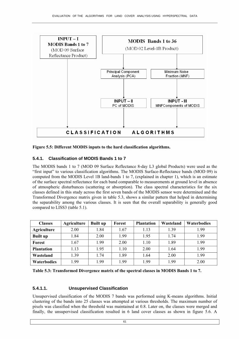
EVALUATION OF THE ALGORITHMS FOR LAND COVER ANALYSIS USING HYPERSPECTRAL DATA
Figure 5.5: Different MODIS inputs to the hard classification algorithms.
L3 global Products) were used as the first input” to various classification algorithms. The MODIS Surface-Reflectance bands (MOD 09) is
ance for each band comparable to measurements at ground level in absence f atmospheric disturbances (scattering or absorption). The class spectral characteristics for the six lasses defined in this study across the first seven bands of the MODIS sensor were determined and the ransformed Div x tab how at e ng
ty amo various es. It n that the overall separability is genISS3 (t .1).
Agr re Built Forest Plantation Wasteland Waterbodies
5.4.1. Classification of MODIS Bands 1 to 7
The MODIS bands 1 to 7 (MOD 09 Surface Reflectance 8-day“computed from the MODIS Level 1B land-bands 1 to 7, (explained in chapter 1), which is an estimate of the surface spectral reflectocT ergence matri given in le 5.3, s s a similar p tern that help d in determinithe separabilicompared to L
ng theable 5
class is see erally good
Classes icultu upAgriculture 2.00 1.84 1.67 1.13 1.39 1.99 Built up 1.84 2.00 1.99 1.95 1.74 1.99 Forest 1.67 1.99 2.00 1.10 1.89 1.99 Plantation 1.13 1.95 1.10 2.00 1.64 1.99 Wasteland 1.39 1.74 1.89 1.64 2.00 1.99 Wat odierb es 1.99 1.99 1.99 1.99 1.99 2.00
Table 5.3: Transformed Divergence matrix of the spectral classes in MODIS Bands 1 to 7.
5.4.1.1.
nsupervised classification of the MODIS 7 bands was performed using K-means algorithms. Initial clustering opixels as finally, the
Unsupervised Classification
Uf the bands into 25 classes was attempted at various thresholds. The maximum number of
w classified when the threshold was maintained at 0.8. Later on, the classes were merged and unsupervised classification resulted in 6 land cover classes as shown in figure 5.6. A
61

EVALUATION OF THE ALGORITHMS FOR LAND COVER ANALYSIS USING HYPERSPECTRAL DATA
histogram gvarious clas
enerated for FCC show 6 peaks, indicating 6 categories of land uses. The statistics for the ses are shown in table 5.4.
Figure 5.6: Unsupervised Classification on MODIS Bands 1 to 7.
pervised Classification
was perform
5.4.1.2. Su
Supervised classification on MODIS bands 1 to 7 ed using Gaussian Maximum Likelihood Clas ie C), pper two tree Approach (DTA).
• C was c ed using ban Red), 2 (NIR) d 4 (Green). The geneous p hes were ide for tr ata collection. T MODIS bands 1 to e classifie GMLC te . At a old of 0.001, th bands gave a good entation o land cover .
• bove band re then cla sing t technique. At ngle of 0.5 radians,
tput of the ssified map also represented the 6 land cover classes.
• s used fo assifying MODIS data of 7 bands. The process the neurons e consum g. Although consi be one of the m
ssification remotely sensed data, y trolling the traini process in NN was lt. Figure shows neu ork R ot. The training cess of the neurons rated 100 mes to see t ergin . The iterations s ped with the overall .09. The mber of hid er wa at 1 and the out activation function pt 0.001. e output act functi increased in ste see the variations
in the classification. The training momentum was initially 0 and was increased gradually.
sif r (GML Spectral Angle Ma (SAM), Neural Ne rk (NN) and Decision
A FC r tea MODIS ds 1 ( anhetero atc ntified aining d he7 werrepres
d byf the
chnique classes
thresh e 7
The a s we ssified u he SAM an athe ou cla
NN wa r cl of training was tim in NN is dered to ost robust techniques for cla of et, con ng difficu 5.7 ral netw MS pl prowas ite 0 ti he conv g point topRMS 0 nu den lay s kept putwas ke Th ivation on was ps to
62

EVALUATION OF THE ALGORITHMS FOR LAND COVER ANALYSIS USING HYPERSPECTRAL DATA
The training RMS exit criteria were 0.1, the training threshold contribution was kept 0.1, and the training rate was maintained 0.2 during the training process.
Figure 5.7: Plot of training RMS vs. iterations of NN applied on MODIS bands 1 to 7.
• Tree approach with s u e k e clas classify the
MODIS 7 bands. Thus, this was a more controlled kind of r of
ence level for each class to control its accuracy. The confidence level shows a feasible way of rules by probability forms, and it also raises a flexibility of data error tolerance. The table also highlights the number of rules used for classification at a confidence level of 0.6. The procedure is described below:
(i) A set of points were defined as training sites based on a priori knowledge of the
study area, for various land cover classes in the data set. (ii) The scaled reflectance values for land cover classes were extracted for the training
data. (iii) The data were converted into SEE5 compatible format and submitted for extraction
of rules. (iv) Since the boosting option changes the exact confidence of the rule, the rules were
extracted without boosting option. A 10% cut off was allowed for pruning the wrong observations.
(v) Once the rules were framed by the SEE5, these rules were ported into Knowledge engineer to make a knowledge based classification schema. It was ensured that 90% confidence level is maintained for all the classes defined.
(vi) Subsequently the decision tree schema was applied over the data set to produce the colour coded land cover output.
Class Rules generated
Confidence level Maximum Minimum
Number of Rules at Confidence level – 0.600
Decision See5 warule based approach
sed by th nowledg sifier to
classification process among all the other techniques. Table 5.4 shows the total numberules generated by the decision tree classifier, the maximum and the minimum confid
63

EVALUATION OF THE ALGORITHMS FOR LAND COVER ANALYSIS USING HYPERSPECTRAL DATA
Agriculture 87 0.982 0.563 87 Built up ( rban/Rural) U
27 0.988 0.551 27
Evergreen/ Semi- 9 0.958 0.667 9 Evergreen Forest Plantation/ orchards 86 0.981 0.648 86 Waste land/Barren Rock / Stony waste
43 0.929 0.253 43
Waterbodies 18 18 0.955 0.625
Table 5.4: Knowledge based Land cover classification of MODIS data (Bands 1 to 7).
The results obtained from the various classification techniqu r MODIS bands 1 to 7 are listed in table 5.5 for comparative analysis. Fro the table it is clear that in the neural network based classification there is an increase in the built up land and plantation classes with a decrease in the waste land percentage. The percentage of vegetation (agriculture, forest and plantation) in K-means clustering was 40.77%, 44.34% (in MLC), 38.06 (in SAM), 49.15% (in NN) and 44.61% (in Decision Tree). The percentage of no terbodies) were
es fom
n-vegetation (built up, waste land/ Barren rock / Stony waste and wafound to be 59.23% in K-means clustering, 55.64% (in MLC), 61.95% (in SAM), 51.13% (in NN) and 55.39% (in Decision Tree) approach respectively. Figure 5.8 shows the corresponding classified images.
Classes K-Means MLC SAM NN Decision Tree
Agriculture (%) 21.13 20.76 17.88 21.88 17.97
Built up (Urban/Rural) (%) 17.83 15.54 20.55 26.44 16.44
Evergreen/ Sem ergreen st (%)
6.85 0.41 7 7.68 13.11 i-EvFore
1 8.3
Plantation/ orc (%) 2.79 3.19 1 19.31 11.53 hards 1 1 11.8
Waste land/Ba ock / ste (%
0.43 9.11 2 24.38 40.23 rren RStony wa )
4 3 40.9
Waterbodies (%) 00.97 00.99 00.47 00.31 00.72
Total (%) 100.00 100.00 100.00 100.00 100.00
Table 5.5: using K-M
Percentage wise distribution of land cover classes for MODIS bands 1 to 7 classified eans, MLC, SAM, NN and Decision Tree Approach.
64

EVALUATION OF THE ALGORITHMS FOR LAND COVER ANALYSIS USING HYPERSPECTRAL DATA
Figure 5.8: Supervised Classification using (A) MLC, (B) SAM, (C) NN and (D) Decision Tree Approach on MODIS Bands 1 to 7.
65

EVALUATION OF THE ALGORITHMS FOR LAND COVER ANALYSIS USING HYPERSPECTRAL DATA
5.4.2. Classification of Principal Components (PC’s) of MODIS Bands 1 to 36
Principal Analysis (PCA) wa ed on MODIS 36 bands (MOD 02 Level-1B Calibrated Data Set) of spatial n e e mamatrix were calculated and eigenvalues are listed in table 5.6.
Eigenvalue
Component Geolocation
s performresolutio 250m. Th covarianc trix and the correlation
PC
1 326014
2 2175
3 1705
4 741
5 189
Table 5.6: Eigenvalue for the PCA analysis of MODIS 36 bands.
It is observed, that only the first few bands have higher information. The first five bands of the PCA were chosen for further analysis based on higher eigenvalues, and the information content that was perceived from visual interpretation of the images through false colour composite. These 5 components were used as the “second input” to the classification algorithms. Transformed Divergence matrix is given in table 5.7 indicated that except built up all other classes are well separable across PC’s. Agriculture Built up Forest Plantation Wasteland Waterbodies Agriculture 2.00 1.10 1.99 1.97 1.99 1.84 Built up 1.10 2.00 1.45 1.35 1.49 1.52 Forest 1.99 1.45 2.00 1.36 2.00 2.00 Plantation 1.97 1.35 1.36 2.00 2.00 2.00 Wasteland 1.99 1.49 2.00 2.00 2.00 2.00 Waterbodies 1.84 1.52 2.00 2.00 2.00 2.00
Table 5.7: Transformed Divergence matrix of the spectral classes in PCs.
• PC’s were first classified by GMLC technique and at a threshold of 0.001, gave the best
representation of the land cover classes. • PC’s were then classified using the Spectral Angle Mapper technique. Here the spectral
2 rest and 0.02 for waterbodies) after iterations of tuning the angle
obtained here was very smooth and the process of training the neurons converg ite n en ayers was kept at 1 and the output activation function was m
that as the num hidden r is increased, the training process takes more tim outp , ma g th en la was j with th t. The
angle was set different for each class (5 for agriculture, 5 for built up, 0.05 for forest, 0.0for plantation, 3 for fobetween the class spectra and the reference spectra to avoid misclassifications.
• Neural Network technique was applied to PC’s. After several iterations of the training
process, stability was achieved. Figure 5.9 shows the NN plot of the training process iteration versus the RMS error obtained. The training curve
ed at 1000 rations. Theaintained at 0.001. It was seen
umber of hiddl
ber of uts. So
layeintainin
e, giving is resulirrelevant e hidd yer at 1 ustified
66

EVALUATION OF THE ALGORITHMS FOR LAND COVER ANALYSIS USING HYPERSPECTRAL DATA
trainingwas ob
mom as i all steps when it served train eu each ility.
entum wthat the
nitially kept 0 and was later on increased in sming of n rons is r ing stab
Figure 5.9: Plot of training RMS vs. iterations of NN applied on PCA bands (MODIS Bands 1 to 36).
Class Rules generated Confidence level Maximum Minimum
Number of Rules at Confidence level – 0.92
• Decision Tree approach using See5 and the knowledge engineer was used to classify PC’s.
For each training site, a level of confidence in characterisation of the site was recorded. Table 5.8 shows the total number of rules generated, the maximum and the minimum confidence level for each class and the number of rules used for classification at a confidence level of 0.92. Here the image was classified into 16 classes initially and were ultimately merged into six categories.
Class 1 49 0.989 0.737 36 Class 2 29 0.997 0.944 20 Class 3 3 0.944 0.833 2 Class 4 2 0.354 0.315 1 Class 5 25 0.985 0.591 11 Class 6 31 0.989 0.800 18 Class 7 31 0.993 0.688 13 Class 8 4 0.875 0.667 1 Class 9 6 0.929 0.800 1 Class 10 2 0.833 0.833 1 Class 11 2 0.929 0.889 1 Class 12 4 0.917 0.875 1 Class 13 2 0.938 0.875 1 Class 14 3 0.963 0.875 1 Class 15 2 0.944 0.833 1 Class 16 3 0.889 0.722 1
Table 5.8: Knowledge based LC classification of PC’s.
The results obtained from these classification techniques are listed in table 5.9. The percentage of vegetation (agriculture, forest and plantation) was 45.56% (in MLC), 43.67 (in SAM), 45.98% (in NN)
67

EVALUATION OF THE ALGORITHMS FOR LAND COVER ANALYSIS USING HYPERSPECTRAL DATA
and 43.12% (in Decision Tree). The percentage of non-vegetation (built up, waste land / barren rock / 54.41% (in MLC), 56.31% (in SAM), 54.00% (in NN)
approach respectively. Figure 5.10 shows the classified images using stony waste and waterbodies) were found to be and 56.88% (in Decision Tree)MLC, SAM, NN and DTA.
Classes MLC SAM NN Decision Tree
Agriculture (%) 25.93 19.78 21.49 22.11
Built up (Urban/Rural) (%) 16.66 11.46 15.78 15.96
Evergreen/ Semi-Evergreen Forest (%)
10.78 10.73 12.04 9.58
Plantation/ orchards (%) 8.85 13.16 09.45 11.43
Waste land/Barren Rock / Stony waste (%)
37.16 44.47 40.33 38.29
Waterbodies (%) 0.62 0.40 0.91 2.63
Total (%) 100.00 100.00 100.00 100.00
Table 5.9: Percentage wise distribution of LC using MLC, SAM, NN and DTA on PC’s.
68

EVALUATION OF THE ALGORITHMS FOR LAND COVER ANALYSIS USING HYPERSPECTRAL DATA
Figure 5.10: Supervised Classification using (A) MLC, (B) SAM, (C) NN and (D) Decision Tree Approach on PC’s.
69

EVALUATION OF THE ALGORITHMS FOR LAND COVER ANALYSIS USING HYPERSPECTRAL DATA
5.4.3. Classification of Minimum Noise Fraction (MNF) components of MODIS Bands 1 to 36
Minimum Noise Fraction (MNF) was performed on the MODIS bands 1 to 36. The covariance matrix, correlation matrix, eigenvectors and eigenvalues were computed for the MNF and the eigenvalues are listed in table 5.10.
MNF Components Eigenvalue 1 91 2 59 3 45 4 29 5 24
Table 5.10: Eigenvalue for the MNF analysis of MODIS 36 bands.
The first five components of MNF were chosen depending on their higher eigenvalues for classification. The output of MNF reflected more information content, yet the image obtained were more pixilated and appeared to be arranged in a brick line fashion in some places on the image. To avoid noise, the other components of MNF were ignored as they that had lower signal-to-noise ratio. These 5 components were used as the “third input” to the various classification algorithms. The Transformed Divergence matrix is given in table 5.11, showed that the overall inter class separability is very high due to reduced noise. Class Agriculture Built up Forest Plantation Wasteland Waterbodies Agriculture 2.00 2.00 1.58 0.96 1.93 1.98 Built up 2.00 2.00 1.99 2.00 1.91 2.00 Forest 1.58 1.99 2.00 1.16 1.51 1.99 Plantation 0.96 2.00 1.16 2.00 1.94 1.99 Wasteland 1.93 1.91 1.51 1.94 2.00 2.00 Waterbodies 1.98 2.00 1.99 1.99 2.00 2.00
Table 5.11: Transformed Divergence matrix of the spectral classes in MNF.
• The pixels in the MNF components were not very distinct and were clustered into mini groups (comprising of two or three pixels). Though, the class separability was very good, yet it was difficult to classify each pixel based on signature, since the image was slightly pixilated. The MNF components were classified by GMLC technique at a threshold of 0.001.
• MNF components were then classified using the SAM technique. At an angle of 5 radians,
all the classes represented the land cover classes well (except water, which was classified at an angle of 0.2 radians).
• NN was used to classify the MNF components. The graph in figure 5.11 was relatively
smooth for the whole process and shows the training process converging at 1000 iterations. The hidden layer was 1 and the output activation function was 0.001. The training momentum was initially 0 and was increased gradually. Other observations were similar to that of PCA classification. The RMS error at the completion of the process was 0.29.
70

EVALUATION OF THE ALGORITHMS FOR LAND COVER ANALYSIS USING HYPERSPECTRAL DATA
Figure 5.11: Plot of training RMS vs. iterations of NN applied on MNF Components.
• Decision Tree approach was used to generate the rules for the knowledge classifier to classify the image. The threshold factor was maintained at 0.7. Table 5.12 shows the total number of rules generated, the maximum and the minimum confidence level for each class and the number of rules used for classification at a confidence level 0.7.
Class Rules generated Confidence level Maximum Minimum
Number of Rules at Confidence level - 0.7
Agriculture 59 0.989 0.500 58
Built up (Urban/Rural)
24 0.996 0.875 25
Evergreen/ Semi-Ever
64 0.995 0.971 63 green Forest
Plantorchards
ation/ 43 0.970 0.667 44
Waste land/ Barren Rock / Stony waste
36 0.993 0.500 36
Waterbodies 5 0.929 0.750 5
Table 5.12: Knowledge based LC classification for MNF components.
The results obtained from these classification techniques are listed in table 5.13. In SAM classification
. The classified images obtained are shown in figure .12
.
there is an increase in the forest and plantation class whereas in ML classification, agriculture is high and on the other hand forest and waterbodies show a relatively low contribution to the land cover class percentage. In the decision tree approach, there is a slight decrease in the water class percentage. Vegetation (agriculture, forest and plantation) contributes 45.37% (in MLC), 46.90% (in SAM), 39.81% (in NN) and 46.29% (in Decision Tree) and non-vegetation (built up, waste land/ Barren rock / Stony waste and waterbodies) contributes 54.96% (in MLC), 53.08% (in SAM), 60.46% (in NN) and 53.71% (in Decision Tree) approach, respectively5
71

EVALUATION OF THE ALGORITHMS FOR LAND COVER ANALYSIS USING HYPERSPECTRAL DATA
Classes MLC SAM NN Decision Tree
Agriculture (%) 26.63 19.55 19.38 21.70
Built up (Urban/Rural) (%) 14.33 12.20 17.55 17.56
Evergreen/ Semi-Evergreen Forest (%)
7.29 14.30 11.32 10.15
Plantation/ orchards (%) 11.12 13.07 10.84 9.44
Waste land/Barren Rock / 40.27 40.21 39.97 40.39 Stony waste (%) Waterbodies (%) 00.36 00.67 00.94 00.76
Total (%) 100.00 100.00 100.00 100.00
Table 5.13: Percentage wise distribution of LC classes obtained from MNF components classification using MLC, SAM, NN and DTA.
72

EVALUATION OF THE ALGORITHMS FOR LAND COVER ANALYSIS USING HYPERSPECTRAL DATA
Figure 5.12: Supervised Classificati g (A) MLC, ) SAM, (C) NN and (D) Decision Tree
NF components. on usin (B
Approach on M
73

EVALUATION OF THE ALGORITHMS FOR LAND COVER ANALYSIS USING HYPERSPECTRAL DATA
T tion of various c with respect to different classification algorithms compared on the basis of percentage area is depicted in Table 5.14. The table shows the uniform distribution of agriculture, forest, plantation and waterbodies classes whereas built up has increased and waste land fell below average line in NN based classification for MODIS Bands 1 to 7.
Agriculture p Forest Waste land Waterbodies (%)
he overall representa lasses
Algorithms (%) (%) (%) (%) (%) Built u Plantation
K-Means (B1 to B7) 21.13 17.83 6.85 12.79 40.43 00.97
MLC (B1 to B7) 20.76 15.54 10.41 13.19 39.11 00.99
SAM (B1 to B7) 17.88 20.55 8.37 11.81 40.92 00.47
NN (B1 to B7) 21.88 26.44 7.68 19.31 24.38 00.31
DTA (B1 to B7) 17.97 16.44 13.11 11.53 40.23 00.72
MLC (PCA) 25.93 16.66 10.78 8.85 37.16 0.62
SAM (PCA) 19.78 11.46 10.73 13.16 44.47 0.40
NN (PCA) 21.49 15.78 12.04 09.45 40.33 0.91
DTA (PCA) 22.11 15.96 9.58 11.43 38.29 2.63
MLC (MNF) 26.63 14.33 7.29 11.12 40.27 00.36
SAM (MNF) 19.55 12.20 14.30 13.07 40.21 00.67
NN (MNF) 19.38 17.55 11.32 10.84 39.97 00.94
DTA (MNF) 21.70 17.56 10.15 9.44 40.39 00.76
T of different algorithms versus percentage a
ixel to a known single land cover class. p ixed pixel e in ttem gh ca IS d seri unda ps, each class considered, instead of a single one depicting all classes present in an ima e, ev el w assigne sively to one class, b , modeled by a linear m
5 ansform
M n was p ed on 8 l Products) used erm inher ension the dat duce n putational requirements sequ cess using e coher ions in subsequent processing, the noise is separated from proving spectral processing r
5.5.2. Endmember collection
T rs were ex direc th witho g exis ectral libraries. The selections of endmembers to train the algorithm were done in several steps.
able 5.14: Land cover classes compared on the basis rea.
5.5. Soft classification: Spectral Unmixing of MODIS imagery
The hard classification techniques discussed above classified each pwith coarse spatial resolution are likelyPixels
roblem of m to have m
g was aore than one
pted throuland cover ty
soft classifipe posing the
tion of MODs. Hence lin ar unmixata. LSU generated a es of ab nce ma one for
ge. Her ery pix as not d excluut was part of many odel.
.5.1. MNF Tr ation
NF transformatio erform the seven bands of the MODIS (MOD 09 Surface Reflectance -day L3 globa . It was to det ine the ent dim ality of a, to reoise and com for sub ent pro ing. By only th ent port
the data, thus imesults.
he endmembe tracted tly from e data ut usin ting sp
74

EVALUATION OF THE ALGORITHMS FOR LAND COVER ANALYSIS USING HYPERSPECTRAL DATA
5.5.2.1. Using Pixel Purity Index (PPI)
The MNF bands were used in the PPI (as explained in chapter 4), processing designed to locate the in
sponded to the number of times that pixel was recorded as the PPI. A threshold was t pixels in order to keep the
o endmembers mix, then the mixed pixels fall in a line in e histogram. The pure endmembers fall at the two ends of the mixing line. If three endmembers mix,
t d pixels f ria r e bers fall inside a tetrahedron, etc. Mixtures of e l in between t em ll spectra erior to endmembi ed by the endmem rti cause al undance sitive and t t of mixed pixels were used to determine how m em re present h g their spec
5 -Dimensio ual n
The spectra are the points in an n-dimen l plot, w is the n of bands. coordinates of the points in n-space consist of ‘n’ that are s the spec ectance vain each band for a given pixel. The distribution of e points pace was estimaten ctral endmembe their sp signatures provided uitive meaunderstand the spectral characteristics of mate ls. The pixels from the spectral ere i n-dimen scatter p rotated on
tool until points emities on the plot were exposed. These projections were rotated in lesser dimensions to
end member) was exported to a ROI in the image. Mean spectra were then extracted for each ROI to act as endmembers for spectral unmixing. These endmembers were then used for subsequent classification and other processing.
5.5.2.4. Training sites obtained from Ground Truths
A few of the training sets were exclusively collected in the field, corresponding to pure pixels. These training data were overlaid on the FCC of the image and a region of interest (ROI) was created, thus enabling direct selection of assumed pure pixels from the images. This was done for all classes (agriculture, built up, forest, plantation, waste land and waterbodies) where a clear distinction between their pixels was possible. Finally, these ROIs obtained by different methods were merged into six classes and exported as endmembers.
5.5.3. Class spectral characteristics of the Endmembers
The spectral characteristics of the endmembers were analysed by plotting the endmembers andobtaining the Transformed Divergence matrix which showed a clear separability between the endmembers. These endmembers were then rotated using the n-dimensional visualiser. Snapshots of the visualisation are shown in figure 5.13. The endmembers are marked using a white circle in figure 5.13
most spectrally pure pixels typically corresponding to mixing endmembers. A PPI image was createdwhich the digital number of each pixel correextreme. A histogram of these images showed the distribution of hits byinteractively selected using the histogram and used to extract only the puresnumber of pixels to be analyzed to be minimum. These pixels were used as input to an interactive visualization procedure for separation of specific endmembers.
5.5.2.2. Using Scatter Plot
Scatter plots of the bands also helped in locating some of the purest endmembers by taking the extreme corner pixels. In two dimensions, if only twthhen the mixe all inside a t ngle, fou ndmemndmembers fil he endm bers. A mixed are int the pure ers, nside the simplex form ber ve ces, be l the ab s are po sum o unity. These se any endm bers we and elped in estimatin tra.
.5.2.3. Using n nal Vis izatio
here nsiona scatter umber The values imply tral refl lues
thes in n-s used to the umber of spe rs and pure ectral , and an int n to
ria
bands wor extr
loaded nto an scatter
sional lot and the visualisation marked using region of interest (ROI) tool and then were repeatedly
etermine if their signatures were unique. Once a set of unique pixels were defined, then each separate dprojection on the scatter plot (corresponding to pure
75

EVALUATION OF THE ALGORITHMS FOR LAND COVER ANALYSIS USING HYPERSPECTRAL DATA
(A). It shows that the endmembers selected for the analysis are well separable and can be distinguished from each other.
Figure 5.13: 3-Dimensional visualisation of the Endmembers showing their separability.
5.5.4. Linear Spectral Unmixing
Linear Unmixing was performed using the endmem er obtained, and keeping the unit sum constraint as 1. Fraction images corresponding to each endmem r were generated. The visual inspection of the fraction images shown in figure 5.14 and figure 5.15 indicates that the LSU algorithm was generally capable to detect the patterns present in the supervised classification, but at the same time incurred in significant errors. The proportions of the endmembers in the fraction image ranges from 0 to 1. 0 indicates absence of the endmember and increasing value shows higher abundance with 1 representing 100% presence of the endmember in a particular pixel. This is evident when looking at the fraction map for Agriculture (figure 5.14 (A)) which has mixed at several places with forest / plantations. The first exhibits an over detection along a wide range of the central portion of the area. Plantation and agriculture seems to have mixed at a few places when compared to the hard classified image. The overall representation of wasteland / barren rock / stone was better and in the case of waterbodies, there is a clear case of false detection of the endmember in the northern region of the district and, particularly in the central portion of the district. By and large, other classes show a better behaviour, with distribution and relative values more closely resembling the outputs of the supervised classification, though still some errors exist.
bbe
76

EVALUATION OF THE ALGORITHMS FOR LAND COVER ANALYSIS USING HYPERSPECTRAL DATA
Figure 5. 14: (A) Gray scale Abundance Maps for Agriculture and (B) Built up land (Urban / ural). R
77

EVALUATION OF THE ALGORITHMS FOR LAND COVER ANALYSIS USING HYPERSPECTRAL DATA
Figure 5.15: Gray scale aps for Evergreen / Semi-Evergreen Forest (A) Plantations/orchards (B) Wasteland/Barren rock/Stone (C) and Waterbodies (D). Bright pixels represent higher abundance of 50% or more stretched from black to white.
Abundance M
78

EVALUATION OF THE ALGORITHMS FOR LAND COVER ANALYSIS USING HYPERSPECTRAL DATA
It has to be y times fell ond acceptable limits, showing highly positive and negative values, usually corresponding to areas
f high RMSE (figure 5.16). In those cases, values that exceeded 1 were considered to be 1 and values k) represents no error and 1 (white)
noted that output values of the different MPF’s (Material Pixel Fractions) manbeyounder 0 were assimilated to this cipher. In figure 5.16, 0 (blacrepresents high error in the fraction image.
Figure 5.16: Overall RMSE for MODIS. Bright pixels represent high error.
w good correspondence between the visual patterns and relative values of
the fractions when compared with the hard supervised classification suggesting a better behaviour in the here are many areas where proportions of agriculture are properly
ametric
Overall, the MPF images sho
distribution of the endmembers. Tpredicted, mainly in the western central portion of the study area however, there is clear underestimation in the south central region of the district. Errors can be seen in the wrong detection of waterbodies showing high discrepancies. As the experimental results show, classes identified in remote-sensing data may exhibit an interclass variability too high to allow the unique linear spectral unmixing of single pixels. Parrepresentation of the constituent pure classes used for linear unmixing does not properly represent local classes since the sampling error may be significant and, in most cases, parametric probability density functions are valid when certain assumptions are met that do not always hold in practice [133]. The variability of the pixels that represent the local pure classes then is responsible for the uncertainity with which the mixture proportions can be identified. The accuracy of these classified images is discussed in chapter 6 (Accuracy Assessment).
79

EVALUATION OF THE ALGORITHMS FOR LAND COVER ANALYSIS USING HYPERSPECTRAL DATA
6. Accuracy Assessment
Image classification results in a raster file in which the individual raster elements are class labelled. As
ent of the LISS-3 MSS classified image (of spatial solution 23.5 m) and MODIS classified image (of spatial resolution 250 m). The chapter is arranged
hard classified maps. This assessment has been done at three levels with the ground truth data collected from the field, at the administrative boundary level (Taluk level)
cronym used in this chapter:
Decision Tree Approach applied on MODIS Bands 1 to 7. 1
Spectral Angle Mapper applied on MNF2 components of MODIS 36 bands. 13. NN (MNF) – Neural Network applied on MNF2 components of MODIS 36 bands.
proach applied on MNF2 components of MODIS 36 bands.
-3 MSS Classification Accuracy
image classification is based on samples of the classes, the actual quality should be checked and quantified afterwards. This is usually done by a sampling approach in which a number of raster elements are selected and both the classification result and the true world class are computed. Comparison is done by creating an error matrix from which different accuracy measures can be calculated. This chapter deals with the accuracy assessmreinto 3 sections. The first section (6.1) discusses the accuracy assessment of the LISS-3 supervised and unsupervised classification. MODIS classification accuracy assessment is shown in second section (6.2). Section 6.2 is further sub-divided into 2 sub sections. The first subsection (6.2.1) discusses the accuracy estimation of the MODIS –and at the pixel level; by comparing on pixel by pixel basis with respect to LISS-3 classified map. The second subsection (6.2.2) shows the accuracy assessment of the soft classification at the administrative boundary level and at the pixel level, compared to LISS-3 classified image. The chapter concludes with a short discussion on the results of hard classification, soft classification and accuracy assessment (section 6.3). A
1. MLC (LISS-3) – Maximum Likelihood classification on LISS-3 MSS. 2. K-Means (B1 to B7) – K- Means Clustering algorithm applied on MODIS Bands 1 to 7. 3. MLC (B1 to B7) – Maximum Likelihood classification on MODIS Bands 1 to 7 4. SAM (B1 to B7) – Spectral Angle Mapper applied on MODIS Bands 1 to 7. 5. NN (B1 to B7) – Neural Network applied on MODIS Bands 1 to 7. 6. DTA (B1 to B7) –7. MLC (PCA) – Maximum Likelihood classification applied on PC of MODIS 36 bands. 8. SAM (PCA) – Spectral Angle Mapper applied on PC1 of MODIS 36 bands. 9. NN (PCA) - Neural Network applied on PC1 of MODIS 36 bands. 10. DTA (PCA) – Decision Tree Approach applied on PC1 of MODIS 36 bands. 11. MLC (MNF) – Maximum Likelihood classification on MNF2 components of MODIS 36 bands. 12. SAM (MNF) –
14. DTA (MNF) – Decision Tree Ap1 PC – Principal Components 2 MNF – Minimum Noise Fraction
6.1. LISS
Accuracy assessment was done for Chikballapur administrative unit (taluk), where field data were collected on 5th September and 25th November 2005. Figure 6.1 shows overview of the Chikballapur taluk and its location in Kolar district. Table 6.1 gives the area of each taluk in hectares.
80

EVALUATION OF THE ALGORITHMS FOR LAND COVER ANALYSIS USING HYPERSPECTRAL DATA
Figure 6.1: Chikballapur taluk in Kolar district where field data were collected.
Taluks Area (in hectares)
Bagepalli 92898 Gudibanda 22727 Gauribidanur 88859 Chikballapur 63821 Sidlaghatta 67057 Chintamani 88904 Srinivaspur 86279 Kolar 79218 Mulbagal 81974 Malur 64500 Bangarpet 86806 Total 823043
Table 6.1: Area statistics of each taluk in Kolar district.
he producer’s and user’s accuracy (as explained in chapter 4) corresponding to the various categories, nd the overall accuracy were computed, along with the error matrices for supervised and unsupervised lassified MSS data of LISS-3, which is summarised in table 6.2 and Annexure D (table 1 and 2). The
LISS-3 supervised classification accuracy assessment gave a kappa (k) value of 0.95 indicating that an observed classification is in agreement to the order of 95 percent.
Unsupervised Classification
Tac
Supervised Classification Category Producer’s
Accuracy (%) (%)
User’s Accuracy (%)
Ovacc
erall uracy (%)
(%)
Producer’s Accuracy (%)
User’s Accuracy (%) (%)
Overall Accuracy (%) (%)Agriculture 94.21 84.54 94.47 83.39
Built up 96.47 83.11 89.68 80.30 Forest 94.73 96.20 86.77 89.71 Plantation 92.27 91.73 84.44 90.10 Waste land 97.49 89.88
93.03 93.37
95.63
90.22
Water 96.13 98.33 92.91 94.89
Table 6.2: Producer’s accuracy, user’s accuracy and overall accuracy of land cover classification using LISS-3 MSS data for Chikballapur Taluk.
81

EVALUATION OF THE ALGORITHMS FOR LAND COVER ANALYSIS USING HYPERSPECTRAL DATA
6.2. MODIS Classification Accuracy
he ground truth data and the results are listed in Table 3, 6.4 and 6.5 respectively.
6.2.1. Accuracy Assessment of hard classification for MODIS
6.2.1.1. Using Error matrix
User’s (3), Producer’s (4) and Overall accuracy assessment of the MODIS classified maps (using hard classifier) was done for Chikballapur taluk with t6. Algorithms Overall Accuracy Rank NN (MNF) 86.11 1MLC (B1 to B7) 75.99 2DTA (MNF) 74.66 3DTA (B1 to B7) 71.89 4NN (PCA) 71.02 5DTA (PCA) 70.10 6SA 1 to B7) 69.41 7M (BNN (B1 to B7) 68.88 8K-Means (B1 to B7) 59.88 9SAM (MNF) 49.27 10MLC (MNF) 42.22 11SAM (PCA) 35.22 12MLC (PCA) 30.44 13
Table
Algor
6.3: Overall Accuracy of classified MODIS Data of Chikballapur taluk.
ithms Agriculture Built up Forest Plantation Waste land Waterbodies
K-Means (B1 to B7) 54.23 75.44 79.57 61.88 82.63 48.07
MLC (B1 to B7) 84.01 84.77 94.21 51.33 84.33 51.49
SAM (B1 to B7) 46.63 71.71 84.05 61.18 87.53 45.61
NN (B1 to B7) 94.00 80.80 94.65 59.40 93.87 45.55
DTA (B1 to B7) 64.44 98.27 89.21 63.35 62.55 88.91
MLC (PCA) 71.22 69.99 89.05 86.48 67.33 64.41
SAM (PCA) 53.44 65.31 88.32 54.97 73.99 61.45
NN (PCA) 97.33 95.18 67.67 95.38 74.07 48.00
DTA (PCA) 63.12 79.11 81.11 69.33 66.29 63.01
MLC 22 85.11 41.22 (MNF) 43.33 61.02 91.23 61.
SAM (MNF) 57.45 49.94 53.22 63.07 81.05 70.34
NN (MNF) 93.89 94.46 89.13 85.60 74.22 59.40
DTA (MNF) 74.44 62.22 74.58 61.37 71.35 55.18
Table
- It is a m actually
6.4: User’s Accuracy of classified MODIS Data of Chikballapur taluk.
easure of commission error indicating the probability that a pixel classified into a given category(3)
represents that category on the ground. (4) - It indicates how well training set pixels of the given cover type are classified.
82

EVALUATION OF THE ALGORITHMS FOR LAND COVER ANALYSIS USING HYPERSPECTRAL DATA
Algorithms Agriculture Built up Forest Plantation Waste land Waterbodies
K-Means (B1 to B7) 73.33 87.48 62.88 41.68 71.19 30.83
MLC (B1 to B7) 76.49 81.66 73.64 36.31 76.82 89.35
SAM (B1 to B7) 63.49 81.53 71.42 27.99 51.61 70.01
NN (B1 to B7) 68.56 56.73 99.00 73.07 96.60 89.53
DTA (B1 to B7) 40.91 93.04 90.71 44.98 71.62 23.36
MLC (PCA) 53.21 69.78 48.26 69.91 92.20 91.11
SAM (PCA) 86.79 86.21 24.52 67.05 33.09 44.07
NN (PCA) 57.55 93.00 94.00 93.00 93.00 73.51
DTA (PCA) 51.93 81.33 86.21 35.47 53.02 36.49
MLC (MNF) 71.66 56.77 45.35 66.13 45.77 99.00
SAM (MNF) 47.66 31.89 31.42 51.01 45.51 67.22
NN (MNF) 69.99 91.89 87.24 99.00 95.00 56.93
DTA (MNF) 49.91 79.66 81.66 83.33 77.09 36.84
Table 6.5: Producer’s Accuracy of classified MODIS Data of Chikballapur taluk.
From the overall accuracy assessment, NN on MNF and MLC classification on MODIS bands 1 to 7 performed better than the other techniques.
6.2.1.2. Comparison based on land cover class percentage area
Accuracy Assessment of MODIS classified maps was also performed at two spatial scales – at the administrative boundary level (Taluk) and at the pixel level. Land cover statistics were computed for all taluks pertaining to each classification algorithm. Land cover percentage area versus various algorithms or Chikballapur is shown in table 6.6. Percentage area statistics for the six land cover classesf were
computed for all the taluks and were compared on the basis of the different algorithms (please see Annexure D, table 3 to table 13). Figure 6.2 shows the best (left) to worst (right) algorithms for land cover class mapping in Chikballapur taluk.
Algorithms Agriculture Built up Forest Plantation Waste land Waterbodies MLC (LISS3) 28.07 11.51 17.06 11.56 31.04 0.76K-Means (B1 to B7) 18.1 19.48 16.45 16.74 28.72 0.03MLC (B1 to B7) 28.31 11.71 16.35 10.4 32.72 0.51SAM (B1 to B7) 48.16 21.38 12.97 14.91 35.38 0.5NN (B1 to B7) 15.83 20.56 11.11 28.37 23.23 0.89DTA (B1 to B7) 18.79 16.99 23.43 9.68 30.72 0.39MLC (PCA) 40.27 7.09 13.06 4.89 34.01 0.68SAM (PCA) 17.4 8.28 15.37 14.96 43.82 0.16NN (PCA) 21.34 0 21.46 8.04 49.03 0.13DTA (PCA) 27.73 24.65 13.9 11.19 21.86 0.67MLC (MNF) 23.72 3.48 14.62 16.1 41.87 0.21SAM (MNF) 30.73 0 28.74 4.02 36.21 0.3NN (MNF) 28.69 10.1 15.72 10.66 34.13 0.7DTA (MNF) 16.08 14.84 25.73 7.06 35.64 0.65
Table 6.6: Land Cover statistics for Chikballapur Taluk.
83

EVALUATION OF THE ALGORITHMS FOR LAND COVER ANALYSIS USING HYPERSPECTRAL DATA
84

EVALUATION OF THE ALGORITHMS FOR LAND COVER ANALYSIS USING HYPERSPECTRAL DATA
Figure land cover classes in
hikballapur taluk. LISS-3 MSS classified image is used for comparison. 6.2: Best (left) to worst (right) classification algorithms for mapping
C
85

EVALUATION OF THE ALGORITHMS FOR LAND COVER ANALYSIS USING HYPERSPECTRAL DATA
The o rall taluk wise percentage area for various algorithms shows that NN based classification on MNF is most comparable to LISS-3 classified
veMODIS image and is suitable for land cover lassification at regional level. MLC on MODIS bands 1 to 7 also proved to be second best algorithm
6.2.1.3
ODIS classified data were also compared with LISS-3 MSS classified data on a pixel by pixel basis
121 pixuser’s a cer’s accuracy and overall accuracy for the taluk and is listed in table 6.7, 6.8 and
.9. This analysis also indicates that NN (MNF) classification technique is relatively better among 13
Algorithms Overall Accuracy Rank
cfor classification.
. Pixel to pixel analysis with LISS-3 MSS classified image
Mfor accuracy assessment of pure (homogenous) pixels. One pixel of MODIS spatially corresponds to
els (that is approximately equal to 258.5 m) of LISS-3. The error matrix was generated with ccuracy, produ
6techniques.
NN (MNF) 69.87 1 MLC(B1 to B7) 65.77 2 NN (PCA) 63.69 3 DTA (MNF) 62.38 4 DTA (PCA) 62.22 5 DTA(B1 to B7) 61.40 6 K-Mea 57.64 7 ns(B1 to 7) SAM(B1 to B7) 56.66 8 MLC (PCA) 53.02 9 SAM ( 51.38 10 PCA) NN(B1 to B7) 51.34 11 SAM (MNF) 47.38 12 MLC (MNF) 41.55 13
Table 6.7: Overall Accuracy obtained from pixel to pixel analysis with LISS-3 image comparison
Algorit Plantation Waste land Waterbodies
for Chikballapur Taluk.
hms Agriculture Built up Forest
86

EVALUATION OF THE ALGORITHMS FOR LAND COVER ANALYSIS USING HYPERSPECTRAL DATA
K-Means (B1 to B7) 41 11 63 56 85 40
MLC ( 51 B1 to B7) 69 39 72 65 85
SAM (B1 to B7) 37 29 75 64 61 49
NN (B1 to B7) 37 17 59 44 87 29
DTA ( 29 49 34 88 48 B1 to B7) 41
MLC (PCA) 36 24 50 48 82 49
SAM ( 64 79 51 PCA) 17 31 71
NN (PCA) 20 45 61 69 81 56
DTA ( 67 82 37 PCA) 34 41 49
MLC (MNF) 40 45 53 69 92 55
SAM (MNF) 21 45 39 61 88 33
NN (M 75 81 65 NF) 41 55 61
DTA (MNF) 31 27 64 61 81 55
.8: User’s Accuracy obtained from pixel to pixTable 6 el analysis with LISS-3 image comparison r Chikballapur taluk.
Algorithms ntation Waste land Waterbodies
fo
Agriculture Built up Forest Pla
K-Means (B1 to B7) 51 44 55 56 62 55
MLC ( 73 66 55 B1 to B7) 45 56 66
SAM (B1 to B7) 41 55 31 54 59 41
NN (B 41 60 45 1 to B7) 46 65 19
DTA (B1 to B7) 51 44 53 67 65 43
MLC ( 61 66 39 PCA) 65 49 32
SAM (PCA) 21 41 29 66 74 37
NN (P 29 38 69 78 45 CA) 61
DTA (PCA) 41 56 38 59 61 42
MLC ( 48 MNF) 58 57 41 57 60
SAM (MNF) 29 55 45 61 61 42
NN (MNF) 59 41 55 76 83 65
DTA ( 58 MNF) 31 44 53 69 71
Table omparison for Chikballapur taluk.
6.9: Producer’s Accuracy obtained from pixel to pixel analysis with LISS-3 imagec
87

EVALUATION OF THE ALGORITHMS FOR LAND COVER ANALYSIS USING HYPERSPECTRAL DATA
6.2.2. Accuracy Assessment of Soft classification for MODIS
6.2.2.1 S-3 MSS
able 6. the abundance maps
orithe area. For the land cover details of each taluk see Annexure D (table 14).
. Comparison on the basis of percentage area with LIS
T 10 shows the land cover statistics for Chikballapur taluk obtained fromgenerated using Linear Mixture Model (LMM), which is compared with LISS-3 classified map. All categ es show comparable values of MODIS to LISS-3 except waterbodies that were overestimated in
Class LMM LISS-3 Agriculture (%) 25.34 28.07 Built up (%) 11.94 11.51 Forest (%) 16.44 17.06 Plantation (%) 12.12 11.56 Waste land (%) 31.83 31.04 Waterbodies (%) 02.33 0.76
The talu y 9 km) gird and homogeneous ure) pixels were verified in each grid. At the pixel level, a total of 51 parcels with respect to the six
provide
Table 6.10: Land Cover details of fraction images for Chikballapur taluk.
6.2.2.2. Accuracy Assessment based on Pixel Analysis
k was divided into 16 quadrants of 5 min by 5 min (9 km b(pland cover classes were verified using handheld Magellan GPS in Chikballapur taluk and table 6.11
s the validation results.
Class Total no. of pixels identified
Pure pixels Mixed pixels Wrongly classified
Agric
ulture 23 18 5 0
Built up 6 4 2 0 (Urban / Rural) EvergEverg
reen / Semi-reen Forest
2 1 1 0
Plantation/Orchards 11 7 4 0
WasteRock
land / Barren / Stony waste
6 4 2 0
Waterbodies 3 1 0 2
Total 5 14 2
51 3
11: Validation of land cover classes in ChikTable 6. ballapur.
Waterbodies which constitute less than 1% of the total area in the district were misclassified and were rongly estimated. Field verification showed that most of the pure pixels as well as few mixed pixels
i
w(for example agriculture with plantations/orchards, open forest class mixed with plantation and barren land m xed with urban class) were classified correctly.
88

EVALUATION OF THE ALGORITHMS FOR LAND COVER ANALYSIS USING HYPERSPECTRAL DATA
6.3. Discussion
6.3.1 Hard Classification
assification technique performs well with high spatial resolution as in the case with LISS-3
.
Hard climage when the actual ground cover is heterogeneous in nature. Good training site and ancillary data, long with minimum difference between the date of acquisition and date of ground truth collection
r uti
urther, cover parameter, errors are generated when the classification algorithm selects
e clas , perhaps as a result of
avoided
dit
.
For Linssentia operly identify different endmembers for MODIS since it proved to be highly relevant, as
attributee land spatial resolution (250 m), where
The reahe results suggest that this could be a limitation to the use of MODIS data in areas of high contrasting
e, en
hen u generate the abundance maps, from the presence of endmembers which do
ot mix in a linear fashion is a
for examfor MO present,
enerally showing the capacity of estimating values within 20 % to 25 % of the actual values.
The Linavoidable. The overall values on the difference maps show only slight divergence, producing good stimates across the whole maps, except for the waterbodies endmembers. It suggest that the selection
vari bilcognizable patterns are found and the RMSE is overall small, it can be deduced that a near perfect
The sperm of equations can be inverted taking the endmember spectra to construct the spectra of each pixel from the original image. Divergences between the original and
afurthe aids in achieving better classification result. MODIS classified image with coarse spatial resol on had many pixels that were misclassified as is clear from the Accuracy Assessment.
within the landFthe wrong class. With respect to a particular class, errors of omission occur when pixels of that class are assigned wrong labels; errors of commission occur when other pixels are wrongly assigned the label of
s considered. These errors occur when the signal of a pixel is ambiguousthspectral mixing, or when the signal is produced by a cover type that is not accounted for in the training process. These errors are a normal part of the classification process. They can be minimized, but not
entirely. As ad ional argument it can be said that as pixel size increases, the chances of high accuracies in hard classifications being product of random assignment of values declines.
6.3.2 Soft Classification using Linear Spectral Unmixing
ear Mixture Modelling (LMM), the selection of the endmembers has an important effect. This is l to pre
it is clear from the results that a high adjacency effect exists between contrasting features (forest and plantation, for example). When comparing LISS-3 MSS and MODIS, another important fact that can be
d to LISS-3 is its spatial resolution (23.5), the reason for its superior results in the detection of cover class distribution and MODIS data having a coarse th
misclassification of the pixels are more likely.
son for the MODIS low accuracy can be the presence of another singularity: adjacency effects. Tnatur as is the case of waterbodies, and raises concerns about its application especially on heavily fragm ted or small isolated areas.
nmixing an image to Wn matter of concern. Errors in sensor operation and sensor noise can also add to the ones already mentioned. These errors take place when the selection of endmembers is wrong,
ple when these do not correspond to pure pixels. The determination of endmember fractions DIS in the study area exhibits good behaviour in places where the endmembers are
g
ear Spectral Unmixing (LSU) of MODIS on the other hand presents more errors which are
efor this endmember could be improved, which is reasonable as this endmember shows high spectral
a ity (for example, clear water is different from turbid water or muddy water). When no more remodel has been reached.
ctra of the different endmembers were modelled by linear equations. This introduces another quality assurance, as thesefo
re
89

EVALUATION OF THE ALGORITHMS FOR LAND COVER ANALYSIS USING HYPERSPECTRAL DATA
reconstructed image also give idea of the goodness of fit of the model, and give insights to which bands e to the errors. add mor
.
When amost im t one is the way of data collection that served as input for the classification of the
ference set.
rensource dLISS-3
een int the training data, the image and validation data are not temporally coincident
MSS (2forma out that time from other sources. Nevertheless, even when counting with a high
utio
lly is representative of the entire classification.
quality orking ith MODIS data, as the quality of its georeferencing could mean a maximum of 10 to 15 % of error in
eaerror ymeasure uncertainty in true geolocation. Therefore, lthough no accurate value can be given, it becomes evident that MODIS subpixel classification
rm
6.3.3 Classification Accuracy
ssessing the accuracies of the image classifications, several things have to be kept in mind. The portan
re Refe ce data include both ground truth data and other ancillary data. The time difference for the
ata used in developing a reference dataset, the reference (field based) date and the MODIS and MSS acquisition dates impact both utility and accuracy of classified maps. Errors may have roduced since b
with the sensor observations. Every possible measure was taken to minimize this effect, relating other ancillary data and vegetation presence information with the visual interpretation of the fused LISS-3
3.5 m) and IRS-1C/1D Panchromatic data (of spatial resolution 5.8 m) and having acquired tion abin
resol n image, which certainly helps to ameliorate the effects of the sampling, care has to be taken in the interpretation of the results, as the presence of bias is likely to happen. To summarize, it is not certain that the reference data in this case actua Another source of bias that influences the conclusions that can be drawn from the classification is the
in the co-registration of the images [134]. This is still a matter of consideration when wwthe ar of a pixel. Although care was taken in the geo-referencing process so as to minimize the RMSE
et, small misregistration may be another significant source of error. Since each MODIS ment is geolocated, this problem amounts to
aperfo ance is definitely better, when mixed pixels are present.
90
EVALUATION OF THE ALGORITHMS FOR LAND COVER ANALYSIS USING HYPERSPECTRAL DATA
7. Conclusions
This study highlights the various preprocssing techniques and the classification algorithms (hard and ed in the research and summarises the results obtained from the accuracy assess
reoft) us sment. The
rch
This wo
eans ier (MLC), Spectral Angle Mapper (SAM), Neural etwork (NN) and Decision Tree Approach (DTA) as well as Linear Mixture Model (LMM) as a soft
product
rincipal Component Analysis (PCA) and Minimum Noise Fraction (MNF) were used to remove the
cover (g tate, India) using ISS-3 (23.5 m spatial resolution) data and MODIS data. LISS-3 data were classified using supervised
inEvergreWaterbo
componLikelihood Classifier, Spectral Angle Mapper, Neural Network and Decision Tree Approach. In the econd phase, 6 fraction images pertaining to each class were generated using the Linear Mixture
l.
he error matrix for LISS-3 classified map showed an overall accuracy of 95.63 % for Chikballapur
maps w
) Error matrices were generated with ground truth data for Chikballapur taluk. The overall aot in ranking with 75.99 % accuracy (see table 6.3 for details). MLC on Principal Components ranked 13th among the techniques with an overall accuracy of 30.44 %.
(ii) Ad hat MLC on MODIS Bands 1 to 7 is best for mapping agriculture and built up. K-Means algorithm was best for mapping forest. Dom
AmaNeural Network classification on MNF components has the highest accuracy of 69.87 % and Mdaf IS classified maps, only 100% pure land cover classes (the matrix of 11 x 11 pixels in LISS-3 classified map) were considered and
sea questions have been answered after an insight in to the findings of the result. Finally the chapter concludes with the scope for further research.
rk compares and assesses the efficacy of various hard classification algorithms namely K-Clustering, Maximum Likelihood ClassifM
Nclassifier for land cover mapping using the MODIS (250 m spatial resolution) surface reflectance
.
Predundancy and noise from the MODIS data. To begin with, NDVI helped in obtaining the general land
reen versus non-green) mapping for study area (Kolar district, Karnataka sLMLC to 6 broader land cover categories (Agriculture, Built up (Urban / Rural), Evergreen / Semi-
en forest, Plantations / orchards, Waste lands / Barren rock/ Stony waste / Sheet rock and dies / Lakes / Ponds / Tanks / Wetland).
In the first phase of experiments, MODIS Bands 1 to 7, PCA-derived components and MNF
ents were classified into the same 6 land cover classes using K-Means clustering, Maximum
sMode
Ttaluk (table 6.2) where field data were collected. Accuracy assessment of the MODIS hard classified
ere estimated at three levels.
(iccuracy, producer’s and user’s accuracy were computed. Neural Network based classification n MNF components showed the best overall accuracy of 86.11 % and MLC on MODIS bands 1 o 7 was the second
comparison of the land cover percentage area among the various classification algorithms was one for Chikballapur taluk (table 6.6). The results showed t
ecision Tree Approach on PCs was found to be good for plantation, while the same technique n MODIS Bands 1 to 7 was best for mapping waste land. Neural Network on MNF component apped the waterbodies accurately.
(iii) t pixel level, MODIS hard classified maps were compared to high resolution LISS-3 classified
ap. The corresponding producer’s, user’s and overall accuracy were computed. This ssessment was in agreement with the error matrix computed using ground truth. It showed that
LC on MODIS Bands 1 to 7 had an accuracy of 65.77 % in decreasing order (see table 6.7 for etails). The other rankings did not tally exactly with the rankings computed using ground truth nd were shuffled to 2 or 3 positions high or low in the rankings. This may be due to the ollowing reasons. While comparing the LISS-3 and MOD
91

EVALUATION OF THE ALGORITHMS FOR LAND COVER ANALYSIS USING HYPERSPECTRAL DATA
twa of the existing hard classification techniques for land cover mapping at regional scale using MODIS data.
The ab at dministrative boundary (taluk level) as well as at pixel levels.
(i.) A n was based on the percentage area of each class with respect to LISS-3 classified map and the percentage of the classes were found to be similar (see table 6.10 f
ATw y/barren (see table 6.11). Waterbodies were overestimated in the study area, indicating requirement of adequate training sites / endmembers representing water cv while mixed pixels were within 20-25% of the actual values. The result shows the utility of spectral unmixing m
he consequence of different spatial scales (at administrative boundary level and at pixel level) on
cover cest but ponents proved to be superior
ixel le dary level. To interpret similar “percentages” from different classifiers
ogion) l analysis gives an
he pre inimum Noise Fraction (MNF) on
results verall lso gave good result and ranked
hoobserva
ISS-3 e data to be normally
on
s well for classifying the image into broader land cover
definiteperform ntage area and the accuracy assessment done at
ixel level (showing good agreement with the LISS-3 classified image as discussed above).
Hyperspsurface features. The classification of MODIS data (of higher spectral and coarse spatial resolution) hows comparable classification accuracy with LISS-3 MSS data (lower spectral and high spatial
hose ranging from 90 – 100 % were neglected. Also, 11 pixels of LISS-3 are 258.5 m spatially, hich is 8.5 m more than the spatial resolution of MODIS pixel (250 m). To summarize, the
bove discussion shows the utility / usefulness
undance maps that could give the fraction of each class in a pixel were also verified
a
t the taluk level, the compariso
or details). The percentage of waterbodies was higher in the abundance map.
(ii.) t the pixel level, the accuracy of the proportions of the classes was validated on the ground. here is mixing of classes in agriculture--plantation/orchards, forest--plantations and built up--aste land/rocky/ston
ategory. MODIS land cover outputs is comparable to LISS-3 classified map, evident from the alidation exercise, as most endmembers (pure pixels) were correctly classified
odel to obtain the abundance maps of the different interpretable classes.
Tclassification accuracy was noticed. When comparing the land cover percentage area among the various algorithms with respect to LISS-3 classified image, it was observed that for mapping a particular land
lass at the boundary level, say for agriculture and built up MLC on MODIS bands 1 to 7 was the when the accuracy was assessed at pixel level, NN on MNF comb
than the other techniques. A certain algorithm may be good for mapping a particular class but at the same time may not be equally good for mapping all other classes. Further, it is recommended to rely on
vel result than at the bounpas an indicator for correct classification is not advisable and reliable. The percentage area of class “A” for tw classifiers may be very similar on an administrative boundary level (i.e. for the entire study
but quite different if the classified images are compared pixel-by-pixel. Pixereidea about the “stability” of classification results.
processing techniques (Principal Component Analysis) and MTMODIS data had different effects on the accuracy of the hard classification algorithms. It was observed that Neural Network (NN) and Decision Tree Approach (DTA) on MNF components give the best
as is evident from their ranking (see table 6.3 for details) which was generated on the basis of accuracy from ground truth. NN and DTA approach on PC’s ao
5th and 6th among the algorithms. The interesting point here is Spectral Angle Mapper and Maximum Likeli od classification that performed worst on the MNF components as well as PCs. The same
tion was made in the accuracy assessment based on pixel to pixel comparison with respect to classified image. One reason for this effect is that NN does not assumL
distributed and DTA uses a non-parametric classification algorithm that involves a recursive partiti ing of the feature space, based on a set of rules learned by an analysis of the training set.
Although, hard classification techniques performcategories having homogeneous surface features, the abundance maps generated from MODIS data is
ly better when considering mixed pixels. The result is evident from the accuracy assessment ed at the taluk level comparison of the perce
p
ectral sensing holds the potential to provide a high spectral data obtained about the earth’s
s
92

EVALUATION OF THE ALGORITHMS FOR LAND COVER ANALYSIS USING HYPERSPECTRAL DATA
resolution) for land cover mapping at a regional level. It is true that the subpixel classification is better rd classifiers for coarse resolution satellite data, yet to what extent this statement holthan ha ds good and
ow far this technique is valid at a global level mapping with high number of endmembers can be a
from Lincludin ixing of MODIS data is lso another area of research along with methods on how to optimize the analysis of the high volumes
virtually
within The mo Mixture Model
LMM). The NLMM takes into account the multiple radiances of the ground cover materials, and thus x
phenom various spectral nmixing applications. NLMM can further be investigated and is the subject of ongoing research.
Study ospectral and spatial resolution. Future research can be carried out to realise the effect of fusion of high patial resolution data and true hyperspectral data (having wavelengths in continuous EM spectrum).
f complexproblem aphazard urban sprawl, global warming, climate change etc.
hsubject of research. Methods can be developed to estimate the accuracy of the fraction images obtained
MM other than ground survey. Use of high resolution classified maps to extract endmembers g techniques like Iterative Error Analysis (IEA), N-FINDR, etc. for unm
aof data acquired. The scope of digital image classification and its application with hyperspectral data is
limitless. Use of neighbourhood operations on classification with the presence of adjacency effects between and
features present on the ground also contribute to heterogeneity and leads to misclassification. st important research area that has not been studied enough is the Non-Linear
(Nthe mi ture is no longer linear. The NLMM has a relatively more accurate simulation of physical
ena and there is not a simple and generic NLMM that can be utilized inu
f vegetation requires species level identification which could be carried out with much higher
sUse o temporal data can further help in understanding land cover dynamics analysis where the
ities of abrupt policy decisions and lack of prior planning have resulted in environmental s like h
93

EVALUATION OF THE ALGORITHMS FOR LAND COVER ANALYSIS USING HYPERSPECTRAL DATA
8. References
] Strahler, A., Muchoney, D., Borak, J., Fried, M., Gopal, S., Lambin, E., and Moody, A., MODIS Land Cover Product, Algorithm Theoretical Basis Document (ATBD). MODIS Land Cover and Land-Cover Change, 1999, Version 5.0.
] Shimazaki, Y., and Tateishi, R., Land Cover Mapping Using Spectral and Temporal Linear Mixing Model at Lake Baikal Region. Paper presented at the 22nd Asian Conference on Remote Sensing, 5 – 9 November 2001, Singapore.
] J.R. Jensen, Remote Sensing of Environment: An earth resource perspective, Pearson Education, 2003.
[4] Natural Resources Census, National Landuse and Land Cover Mapping Using Multitemporal
AWiFS), Project Manual, Remote Sensing & GIS Applications Area, ng Agency, Department of Space, Government of India, Hyderabad,
[5] Wu, C, 1991, www.gisdevelopment.net/aars/acrs/2000/ts12/laus0008.shtml
IST. 10:30]
M., and Townshend, J. R. G., Global discrimination of land cover types from metrics derived from AVHRR Pathfinder data. Remote Sensing of Environment, 1995,
in Israel. International Journal of Remote Sensing, 2001, vol. 12, pp. 500 - 520.
Ustin, S. L., DiPietro, D., Olmstead, K., Underwood, E., and Scheer, G. J., Hyperspectral
[1
[2
[3
AWiFS Data (LULC – National Remote SensiApril 2005.
[last accessed: 21st December, 2005, [6] Townshend, J. R. G., Justice, C. O., Skole, D., Malingreau, J. P., Cihlar, J., Teillet, P.,
Sadowski, F., and Ruttenberg, S., The 1 km AVHRR global data set: needs of the International Geophere Biosphere Programme. International Journal of Remote Sensing, 1994, vol. 15(17), pp. 3417 - 3441.
[7] Defries, R. S., Hansen,
vol. 54, pp. 209 - 222. [8] http://www.oekodata.com/pub/mapping/manual/annexII.pdf.
[last accessed: 21st December, 2005, IST. 10:35] [9] http://glcf.umiacs.umd.edu/index.shtml
[last accessed: 21st December, 2005, IST. 10:35] [10] Clark, R. N., Swayze, G. A., Mapping minerals, amorphous materials, environmental materials,
vegetation, water, ice, snow and other materials: The USGS tricorder algorithm. Summaries of the Fifth Annual JPL Airborne Earth Science Workshop, JPL Publication 1, 1995, pp. 39 - 40.
[11] Ben-Dor, E., Patinand, K., Banin, A., and Karnieli, A., Mapping of several soil properties using
dais-7915 hyperspectral scanner data. A case study over clayey soils
[12]
Remote Sensing for Invasive Species Detection and Mapping. IEEE Transactions on Geoscience and Remote Sensing, 2002, vol. 36(4), pp. 1568–1660.
[13] Goodenough, D. G., Pearlman3, J., Chen1, H., Dyk, A., Han Tian., Li. J., Miller, J., and
Niemann, K. O., Forest Information from Hyperspectral Sensing. IEEE Transactions on Geoscience and Remote Sensing, 2004, vol. 36(4), pp. 2582–2589.
94

EVALUATION OF THE ALGORITHMS FOR LAND COVER ANALYSIS USING HYPERSPECTRAL DATA
[14] Bachmann, C. M., Ainsworth, T. L., and Fusina, R. A., Improvements to Land-Cover and
Invasive Species Mapping from Hyperspectral Imagery In the Virginia Coast Reserve. IEEE
E Transactions on Geoscience and Remote Sensing, 1989, vol. 27(4), pp. 145–153.
G., Justice, C. O., Li, W., Gurney, C., and McManus, J., Global land cover nsing: Present capabilities and future possibilities. Remote Sensing
d cover classifications at a global scale. , vol. 5, pp. 3567 - 3586.
on, P. E., Spectral mixture modelling: A new analysis of rock
aivinen, R. T., Subpixel measurement of tropical forest vol. 12 (5), pp. 1119
[23]
sensor evaluation of an open canopy. IEEE Transaction on Geoscience and Remote Sensing, 1994, vol. 32(5), pp. 1067 - 1080.
Transactions on Geoscience and Remote Sensing, 2004, vol. 36(4), pp. 4180 – 4183. [15] Kerle, N., Janssen, L.L.F., and Huurneman, G.C., Principles of Remote Sensing, ITC
Educational Textbook Series, The International Institute for Geo-Information Science and Earth Observation (ITC), Enschede, The Netherlands, 2004, ISBN 90-6164-227-2. ISSN 1567-5777 ITC Educational Textbook Series.
[16] Salomonson, V. V., Barne, W. L., Maymon, P. W., MODIS: advanced facility instrument for
studies of the earth as a system. IEE
[17] Townshend, J. R.
classification by remote seof Environment, 1991, vol. 35, pp. 243 - 255.
18] DeFries, R. S., Townshend, J. G. R., NDVI derived lan[
International Journal of Remote Sensing, 1994 [19] Lillesand, T.M. and Kiefer. R. W., Remote Sensing and Image Interpretation, Fourth Edition,
John Wiley and Sons, 2002, ISBN 9971-51-427-3.
[20] Loveland, T. R., Zhu, Z., Ohlen, D. O., Brown, J. F., Reed, B. C., Yang, L., An analysis of the global land cover characterization process. Photogrammetric Engineering and Remote Sensing, 1999, vol. 65(9), pp. 1021 - 1031.
[21] Adams, J. B., Smith, M. O., Johnsand soil types at the Viking Lander 1 site. Journal of Geophysical Research, 1986, vol. 91, pp. 8098 - 8112.
[22] Cross, M., Settle, J. J., Drake, N. A., P
cover using AVHRR data. International Journal of Remote Sensing, 1991,- 1129.
Gong, P., Miller, J. R., Spanner, M., Forest canopy closure from classification and spectral unmixing of scene components - multi
[24] Hlavka, C. A., Spanner, M. A., Unmixing AVHRR imagery to assess clear cuts and forest
regrowth in Oregon. IEEE Transaction on Geoscience and Remote Sensing, 1995, vol. 33(4), pp. 788 - 795.
[25] Smith, M. O., Ustin, S. L., Adams, J. B., and Gillespie, A. R., Vegetation in deserts: A regional
measure of abundance from multispectral images. Remote Sensing Environment, 1990, vol. 31 (1), pp. 1 - 26.
[26] Strang, G., Linear algebra and its applications, New York: Academic Press, 1980. [27] Montgomery, D., Peck, E. A., Introduction to Linear Regression Analysis, New York: John
Wiley & Sons, 1982.
95

EVALUATION OF THE ALGORITHMS FOR LAND COVER ANALYSIS USING HYPERSPECTRAL DATA
[28] Anoraks, D. G., Ingle, V. K., and Kogon, S. M., Statistical and adaptive signal processing:
. S., Salomonson, V. V., Prelauch characteristics of MODIS on EOS-AM1. IEEE Transaction on Geoscience and Remote Sensing, 1998, vol. 36(4), pp. 1088–1100.
Running, S., Salomonson, V. V., Terrestrial remote sensing, science and algorithms planned for IS. International Journal of Remote Sensing, 1994, vol. 15(17), pp. 3587–3620.
es IEEE Transaction on Geoscience and Remote Sensing, 1992, vol. 30(1), pp. 2 -
ote%20Sensing.htmDecember, 2005, IST. 10:45]
ber, 2005, IST. 10:45]
http://modis.gsfc.nasa.gov/data/dataprod/dataproducts.php?MOD_NUMBER=09
Guenther, B., Godden, G. D., Pre-launch algorithm and data format for level 1 calibration saction on Geoscience and Remote Sensing,
.
http://daac.gsfc.nasa.gov/MODIS/Aqua/product_descriptions_modis.shtml#rad_geo
Jagadeesh, K., Rao, G.R., Kiran, M.K., Jagadish, K.S. and Ramachandra, T.V, Mapping of Fuel IS.
(http://wgbis.ces.iisc.ernet.in/energy/ paper/)
ote
cst.ssai.biz/mcstweb/calib/reflective.html :50]
w .mcst.ssai.biz/m tweb/ca b/spect l.html ce ed: 21s December, 2005, IST. 10:50]
[44] http://www.mcst.ssai.biz/mcstweb/calib/calibration.html
Spectral estimation, Signal modelling, Adaptive filtering and Array processing, New York: McGraw-Hill, 2000.
29] Barne, W. L., Pagano, T[
[30]
EOS/MOD [31] King, M. D., Kaufman, Y. J., Remote sensing of clouds, aerosol, and water vapours properti
from MODIS. 27.
[32] http://eobglossary.gsfc.nasa.gov/Library/AskScientist/askscientist_5.html [last accessed: 21st December, 2005, IST. 10:45] [33] http://www.scs.gmu.edu/~helaskar/Dust_Web/Rem [last accessed: 21st [34] http://edcimswww.cr.usgs.gov/pub/imswelcome/ [last accessed: 21st Decem [35] [last accessed: 21st December, 2005, IST. 10:45] [36]
products for the EOS-AM1 MODIS. IEEE Tran1998, vol. 36(4), pp. 1142–1151
[37] [last accessed: 21st December, 2005, IST. 10:48] [38] http://modis.gsfc.nasa.gov/data/dataprod/dataproducts.php?MOD_NUMBER=02 [last accessed: 21st December, 2005, IST. 10:49] [39]
Wood Trees in Kolar District Using Remote Sensing Data and G
[last accessed: 21st December, 2005, IST. 10:49] [40] Te-Ming, Tu., Chen, C-H., Wu, J-L. and Chang, C-I., A Fast Two-Stage Classification Method
for High-Dimensional Remote Sensing Data. IEEE Transaction on Geoscience and RemSensing, January 1998, vol. 36(1), pp. 182 – 191.
[41] http://www.mcst.ssai.biz/mcstweb/calib/emissive.html
[last accessed: 21st December, 2005, IST. 10:50] 42] http://www.m[
[last accessed: 21st December, 2005, IST. 10
[43] http://w w cs li ra[last ac ss t
96

EVALUATION OF THE ALGORITHMS FOR LAND COVER ANALYSIS USING HYPERSPECTRAL DATA
[last accessed: 21st December, 2005, IST. 10:50] [45] Richards, J.A., and Jia, X., Remote Sensing Digital Image Analysis - An Introduction, Third
Edition, Springer, May 1996.
Gao, B.C., Heidebrecht, K.B. and Goetz., A.F.H., Derivation of Scaled Surface Reflectance from AVIRIS Data. Remote Sensing of Environment, 1993, vol. 44, pp. 165 – 178.
Anderson, G.P., Wang, J., and Chetwynd, J.H., MODTRAN3: An update and Recent
thm Technical Background Document, Atmospheric Correction Algorithm: Spectral Correction Reflectances (MOD 09), April, 1999, Version 4.0, NASA contract NAS5-96062.
Roberts, D.A., Yamaguchi, Y., and Lyon, R.J.P., Calibration of Airborne Imaging Spectrometer Data to percent Reflectance Using Field Spectral Measurements, 19th International Symposium on Remote Sensing of Environment, Ann Arbor, Michigan, October 21 – 25, 1985.
National Remote Sensing Agency, Hyderabad, India. http://www.nrsa.gov.in/engnrsa/products/geninformation.html [last accessed: 21st December, 2005, IST. 10:55]
Green A. A. and Craig, M.D., Analysis of Aircraft Spectrometer Data with Logarithmic Residuals, Proc. AIS workshop, JPL Publications 85 – 41, Jet Propulsion Laboratory, Pasadena, California, April 8 – 10, 1985, pp. 111- 119.
Kauth, R. J., and Thomas G. S., The tasseled cap—A graphic description of the spectral-temporal development of agricultural crops as seen by Landsat. Symposium Proceedings on Machine Processing of Remotely Sensed Data, June 29 - July 1, 1976, West Lafayette, IN, pp. 41–51.
Jackson, R. D., Spectral indices in n-space. Remote Sensing of Environment, 1983, vol. 13, pp. 409–421.
Ingebritsen, S.E. and Lyon, R. J. P., Principal Components Analysis of Multitemporal Image Pairs. International Journal of Remote Sensing, 1985, vol. 6(5), pp. 687- 696.
Green, A.A., Berman, M., Switzer, P., Craig, M.D., A transformation for ordering multispectral data in terms of image quality with implications for noise removal. IEEE Transactions on Geoscience and Remote Sensing, 1988, vol. 26(1), pp. 65-74.
Research Systems Inc., Minimum Noise Fraction (MNF). Exploring EVNI-an RSI Training course for ENVI 3.0, 1998, pp. 111-114.
Kruse, F. A., Richardson, L. L., and Ambrosia, V. G., Techniques Developed for Geologic Analysis of Hyperspectral Data Applied to Near-Shore Hyperspectral Ocean Data. Presented at the Fourth International Conference on Remote Sensing for Marine and Coastal Environments, Orlando, Florida, 17 – 19 March, 1997.
[46]
[47]
Validations against Airborne High Resolution Interferometer Measurements, 5th Annual JPL Airborne Sciences Workshop, 1995, vol.1 (AVIRIS Workshop), pp. 5 – 8.
[48] Gao, B.C., Heidebrecht, K.B. and Goetz., A.F.H., Atmospheric Removal Program (ATREM)
User Guide, 1992, Centre for the Study of Earth from Space, University of Colorado, Boulder. [49] Vermote, E. F., and Vermeulen, A., MODIS Algori
[50]
[51]
[52]
[53]
[54]
[55]
[56]
[57]
[58]
97
EVALUATION OF THE ALGORITHMS FOR LAND COVER ANALYSIS USING HYPERSPECTRAL DATA
[59] Lee, J.B., Woodyatt, A.S., Berman, M., Enhancement of high spectral resolution remote sensing data by a noise-adjusted principal components transform. IEEE Transaction on Geoscience and Remote Sensing, 1990, vol. 28(3), pp. 295-304.
Chen, C-M., Comparison of principal component analysis and minimum noise fraction transformation for reducing the dimensionality of hyperspectral imagery. Geographical Research, 2000, vol. 33(1), pp. 163-178.
[61] Ramachandra, T.V. and Uttam Kumar, Image Fusion in GRDSS for Land Cover Mapping, Map
India 2005, New Delhi, 7 – 9 February, 2005.
. L., Sharman, M. J., and Van Ittersum, T., Satellite remote sensing of ss production in the Senegalese Sahel: 1980-1984. Remote Sensing
Environment, 1985, vol. 17, pp. 233 – 249.
ing of surface reflectance, SPIE, 1984, vol.
., Kaufman, Y. J., and Mahoney, R. L., Satellite measurements of aerosol mass and
N., and Fraser, R. S., Red and near IR sensor response to off-nadir viewing.
p. 1511 –
by
m value composite images for temporal AVHRR data. 1986, vol. 7, pp. 1417 – 1437.
sing. International Journal of Remote Sensing, 1987, vol. 8, pp. 839 – 857.
Kaufman, Y. J., and Tanre, D., Atmospherically Resistant Vegetation Index (ARVI) for EOS-on on Geoscience and Remote Sensing, 1992, vol. 30(2), pp. 261 –
270.
arkham, B., Dye, D. G., Dulaney, W., and Yang, J., Normalized Difference n Index Measurements from the Advanced Very High Resolution Radiometer.
Woodcock, C. E., and Hamdi, H., The status of agricultural lands in Egypt: The multitemporal NDVI features derived from Landsat TM. Remote Sensing of
[60]
[62] Tucker, C. J., Vapraet, C
total herbaceous bioma
[63] Kaufman, Y. J., Atmospheric effect on remote sens475, pp. 20 -33.
[64] Fraser, R. S
transport, Journal of Atmospheric Environment, 1984, vol. 18, pp. 2577 – 2584. [65] Holben, B.
International Journal of Remote Sensing, 1984, vol. 5, pp. 145 – 160. [66] Holben, B. N., Kaufman, Y. J., and Kendall, J. D., NOAA-11 AVHRR visible and near-IR
inflight calibration bands. International Journal of Remote Sensing, 1990, vol. 11, p1519.
[67] Kaufman Y. J. and Holben, B. N., Calibration of the AVHRR visible and near-IR bands
atmospheric scattering, ocean glint and desert reflection. International Journal of Remote Sensing, 1992.
[68] Holben, B. N., Characteristics of maximu
International Journal of Remote Sensing, [69] Tanre, D., Holben, B. N., and Kaufman, Y. J., Atmospheric correction algorithm for NOAA-
AVHRR products, theory and application. IEEE Transaction on Geoscience and Remote Sensing, 1992, vol. 30.
[70] Kaufman, Y. J., The effect of subpixel clouds on remote sen
[71]
MODIS. IEEE Transacti
[72] Goward, S. N., M
VegetatioRemote Sensing Environment, 1990, vol. 35, pp. 257 – 277.
[73] Lenney, M. P.,
use of Environment, 1996, vol. 56(1).
98

EVALUATION OF THE ALGORITHMS FOR LAND COVER ANALYSIS USING HYPERSPECTRAL DATA
[74] Reed, B.D., Brown, J.F., VanderZee, D., Loveland, T.R., Merchant J.W. and Ohlen, D.O., Measuring phenological variability from satellite imagery. Journal of Vegetation Science, 1994, vol. 5, pp. 703-714.
[75] DeFries, R., Hanson, M., Townshend, J., and Sohlberg, R., Global land cover classifications at
8 km spatial resolutions: The use of training data derived from Landsat imagery in decision tree classifiers. International Journal of Remote Sensing, 1998, vol. 19(6), pp. 3141-3168.
[76] Lambin, E. F. and Ehrlich, D., The surface temperature-vegetation index space for land cover
and land-cover change analysis. International Journal of Remote Sensing, 1996a, vol. 17(3), pp. 463–487.
[77] Lambin, E. F. and Ehrlich, D., Broad scale land-cover classification and interannual climatic
variability. International Journal of Remote Sensing, 1996b, vol. 17(5), pp. 845–862. [78] Townshend, J. R. G., Justice, C. O., and Kalb, V. T., Characterization and classification of
South American land cover types using satellite data. International Journal of Remote Sensing, 1987, vol. 8, pp. 1189–1207.
tween Remotely
enological classification of terrestrial vegetation cover using shortwave imagery. International Journal Remote Sensing, 1990, vol. 11, pp. 2269 –
Belward, A. (ed.), The IGBP-DIS Global 1-km Land Cover Data Set DISCover. IGBP-DIS
[79] Koomanoff, V. A., Analysis of Global Vegetation Patterns: A Comparison beSensed Data and a Conventional Map. Biogeography Research Series, 1989, Report #890201, Department of Geography, University of Maryland.
[80] Lloyd, D., A ph
on index vegetati2279.
[81] Sellers, P., Tucker, C. J., Collatz, G. J., Los, S. O., Justice, C. O., Dazlich, D. A., and Randall,
D. A., A global 1° by 1° NDVI data set for climate studies. Part 2. The generation of global fields of terrestrial biophysical parameters from the NDVI. International Journal of Remote Sensing, 1994.
[82] Belward, A., and Loveland, T. R., The IGBP 1-km land cover project. In Proceedings of the
21st Annual Conference of the Remote Sensing Society, Southampton, UK, 1995, pp. 1099–1106.
[83]
Working Paper, 1996. [84] Eidenshink, J. C., and Faundeen, J. L., The 1-km AVHRR global land data set: First stages in
implementation. International Journal of Remote Sensing, 1994, vol. 15, pp. 3443–3462. [85] Duggin, M. J., Piwinski, D., Whitehead, V., and Ryland, G., Scan-angle dependence of
radiance recorded by the NOAA-AVHRR. Advanced Remote Sensing, Proceedings SPIE, Aug. 26–27, 1982, San Diego, CA, 363, pp. 98–101.
[86] Zhu, Z-L., and Yang L., Characteristics of the 1-km AVHRR data set for North America.
International Journal of Remote Sensing, 1996, vol. 17, pp. 1915–1924. [87] Cihlar, J., Identification of contaminated pixels in AVHRR composite images for studies of
land biosphere. Remote Sensing of Environment, 1996, vol. 56, pp. 149–163.
99
EVALUATION OF THE ALGORITHMS FOR LAND COVER ANALYSIS USING HYPERSPECTRAL DATA
[88] Van Dijk, A., Calhs, S. I., Sakamoto, C. M., and Decker, W. I., Smoothing vegetation index
ent
Foody, G. M., McCulloch, M. B., and Yates, W. B., The Effect of Training Set and
[92]
[93] S., and Townsend, J. R. G., NDVI-derived land cover classification at a global
scale. International Journal of Remote Sensing, 1994, vol. 15(17), pp. 3567 – 3586.
Gopal, S., Sklarew, D. M. and Lambin, E., Fuzzy-neural networks in multitemporal classification of land cover change in the Sahel. New Tools for Spatial Analysis, Proc. of the Workshop, Lisbon, 18 to 20 November, 1993, Office for Official Publication of European Communities, Luxembourg, pp. 69 – 81.
Hepner, G. F., Logan, T., Ritter, N., and Bryant, N., Artificial neural network classification using a minimal training set: Comparison to conventional supervised classification. Photogrammetric Engineering and Remote Sensing, 1990, vol. 56(4), pp. 469 – 473.
Fitzgerald, R. W. and Lees, B. G., Assessing the classification accuracy of multisource Remote Sensing data. Remote Sensing of Environment, 1994, vol. 47, pp. 362 – 368.
Benediktsson, J. A., Swain P. H., and Ersoy, O. K., Neural network approaches versus statistical methods in classification of multisource remote sensing data, IEEE Transactions on Geoscience and Remote Sensing, 1990, vol. 28(4), pp. 540–552.
Lee, J., Weger, W. C., Sengupta, S. K., and Welch, R. M., A neural network approach to cloud classification. IEEE Transactions on Geoscience and Remote Sensing, 1990, vol. 28, pp. 846 - 855.
Yoshida, T. and Omatu, S., Neural network approach to land cover mapping. IEEE Transactions on Geoscience and Remote Sensing, 1994, vol. 32, pp. 1103–1110.
00] Hara, Y., Atkins, R. G., Yueh, S. H., Shin, R. T., and Kong, J. A., Application of neural networks to radar image classification. IEEE Transactions on Geoscience and Remote Sensing, 1994, vol. 32, pp. 100 –111.
profiles: An alternative method for reducing radiometric disturbance in NOAA/AVHRR Data. Photogrammetric Engineering and Remote Sensing, 1987, vol. 53, pp. 1059–1067.
[89] Kruse, F., The Spectral Image Processing Systems (SIMS) – Interactive Visualization and
Analysis of Imaging Spectrometer Data. Remote Sensing of Environment, 1993, vol. 44, pp. 145 – 163.
90] Girouard, G., and Bannari, A., (Remote Sensing and Geomatics of the Environm[
Laboratory, Department of Geography, University of Ottawa, Ottawa-Carleton Geoscience Center, Ontarioa), Harti, A. E., (Remote Sensing and GIS Applied to Geosciences and the Environment, Morocco, University of Cadi Ayyad), and Des rochers, A., (Department of Earth Science, University of Ottawa, Ottawa-Carleton Geo-Science Center), Validated Spectral Angle Mapper Algorithm for Geological Mapping: Comparative Study between Quickbird and Landsat-TM.
[91]
Composition on Neural Network Classification. International Journal of Remote Sensing, 1995, vol. 16 (9), pp. 1707 – 1723.
Moody, A., Gopal, S., and Strahler, A. H., Artificial Neural Network Response to Mixed Pixels
in Coarse Resolution Satellite Data. Remote Sensing of Environment, 1996, vol. 58, pp. 329 – 343.
Fischer, R.
[94]
[95]
[96]
[97]
[98]
[99]
[1
100

EVALUATION OF THE ALGORITHMS FOR LAND COVER ANALYSIS USING HYPERSPECTRAL DATA
[101] Tzeng, Y. C., Chen, K. S., Kao, W.-L., and Fung, A. K., A dynamic learning neural network for remote sensing applications. IEEE Transactions on Geoscience and Remote Sensing, 1994, vol. 32, pp. 1096–1103.
ain, P. H., and Ersoy, O. K., Conjugate-gradient neural networks in urce and very-high-dimensional remote sensing data. International
[103] Carpenter, G., Gjaja, M., Gopal, S., and Woodcock, C., ART Neural Networks for Remote
EE Transactions on Geoscience and Remote Sensing, 1997, vol. 35(2), pp 308–325.
., and Prinz, A. J., Multispectral classification of Landsat-images using neural networks. IEEE Transactions on Geoscience and Remote Sensing, 1992, vol. 30,
482–490.
Neural on of Remotely-Sensed Multi-Spectral Imagery. International Journal vol. 16 (16), pp. 3033 – 3058.
ang, C-C., Prasher, S. O., W ry for nology. Biosystem
classification of remotely sensed data. Paper 001, Singapore.
ethods for remotely sensed data, New York: McGraw-
[110] Stein, A., Aryal, J., and Gort, G., Use of the Bradley-Terry Model to Quantify Association in Remote Sensing, 2005, vol.
., Yu, X., Multi-dimensional signal processing for electrooptical target ernatinal Society for Optical Eng, 1990, vol. 1305, pp. 1-7.
Goetz, A. F. H., Boardman, J. W., Discrimination among semi-arid landscape endmembers using the spectral angle mapper (SAM) algorithm, Summaries 3rd Annual JPL
op, 1, 1992, pp. 147–149.
and a delusion. International Journal of Remote Sensing, 1997,
1 , J. J., D N. A., Line mixing and the estimation of ground cover proportion, ote S sing, 1993 , pp
[116] ent, J. T., M . V., Sp sification fuzzy me models. IEEE Trans.
[102] Benediktsson, J. A., Swclassification of multisoJournal of Remote Sensing, 1993, vol. 14, pp. 2883–2903.
Sensing: Vegetation Classification from Landsat TM and Terrain Data. IE
[104] Bischof, H., Schneider, W
pp.
, J. D., and Schowengerdt, R. A., A review and Analysis of Backpropagation[105] PaolaNetworks for Classificatiof Remote Sensing, 1995,
Y halen, J., and Goel, P. K, Use of Hyperspectral Image[106] Identification of Different Fertilisation Methods with Decision-tree TechEngineering, 2002, vol. 83(3), pp. 291 – 298.
07] Pal, M., and Mather, P. M., Decision Tree based[1
presented at the 22nd Asian conference on Remote Sensing, 5-9 November 2 108] Tso, B., Mather, P. M., Classification m[
Hill, Taylor and Francis, 2001. [109] Campbell, J.B., Introduction to Remote Sensing, Taylor and Francis, New York, 2002.
Remote Sensed Images. IEEE Transaction on Geoscience and43(4), pp. 852-856.
[111] Bosdogianni, P., Petrou, M., and Josef, K., Mixture Models with Higher Order Moments. IEEE
Transaction on Geoscience and Remote Sensing, 1997, vol. 35(2), pp. 341-353.
k .[112] Stoc er, A. D , Reed, I. Sdetection. Proc. SPIE Int
Yuhas, R. H., [113]
Airborne geoscience Worksh
Fisher, P., The pixel: a snare [114]vol. 18(3), pp. 679-685.
[ 15] Settle
International Journal of Remrak, ar
en , vol. 14 (6) . 1159–1177.
KPattern Anal. Machine Intell, 1986, vol. 10(4), pp. 659–671.
ardia, K ectral clas using mbership
101
EVALUATION OF THE ALGORITHMS FOR LAND COVER ANALYSIS USING HYPERSPECTRAL DATA
[117] oardman, J. W., Kruse, F. A ted spectral analysis: a geologic example using AVIRIS
ata, north mount ada, Proc. 10th Thematic Conf. on Geologic Remote Sensing, Environmental Research Institute of Michigan, 1994.
ique for extrapolation and validating
[120]
ing multispectral data, IEEE Transactions on Geoscience and
21 nderstanding and visualization of hyperspectral data as a convex set SPIE symposium on Imaging Spectrometry, Orlando, Florida, 1995,
[122 n Determining End-members in
Sensing, 2000.
sis. IEEE Transactions on ote Sensing, 2000, vol. 38 (2), pp. 1083-1094.
ata Analysis. IEEE Transaction on Geoscience and Remote Sensing, 2002, vol. 40 (12), pp. 2692-2699.
[126 ., Linear mixture modelling for quantifying ing time series NDVI data, GIS Development, New Delhi.
Y. H., Spectral Mixture Analysis of Hyperspectral Data, Department of Surveying Engineering, National Cheng Kung University, Tainan, China Taipei,
ce on Remote Sensing, 5 – 9 November, 2001, Singapore.
Neville, R. A., Levesque, J., Staenz, K., Nadeau, C., Hauff, P., and Borstad, G. A., Spectral unmixing of hyperspectral imagery for mineral exploration: comparison of results from SFSI and AVIRIS. Canadian Journal of Remote Sensing, 2003, vol. 29(1), pp. 99-110.
B ., Automad grapevine ains, Nev
118] Inverson, L.R., Cook, E. A., and Graham, R. L., A techn[
forest cover across large regions: calibrating AVHRR data with TM data. International Journal of Remote Sensing, 1989, vol. 10, pp. 1805-1812.
[119] Quarmbay, N., Townshend, J., Settle, J., White, K., Milnes, M., Hindle, T., Silleos, N., Linear
mixture modelling applies to AVHRR data for crop area estimation. International Journal ofRemote Sensing, 1991.
Shimabukuro, Y. E., and Smith, A. J., The least-squares mixing models to generate fraction images derived from remote sensRemote Sensing, 1991, vol. 29(1), pp. 16–20.
[1 ] Boardman, J., Analysis, u
in n-space. International pp. 23-36.
] Winter, M. E., and Winter, E. M., Comparis o of Approaches for Hyperspectral Data. IEEE Transaction on Geoscience and Remote
[123] Bateson, C. A., Asner, G. P., and Wessman C. A., Endmember Bundles: A New Approach to
Incorporating Endmember Vairability into Spectral Mixture AnalyGeoscience and Rem
[124] Settle, J., On the effect of Variable Endmember Spectra in the Linear Mixture Model. IEEE
tion on Geoscience and Remote Sensing, 2006, vol. 44 (2), pp. 389-396. Transac [125] Dundar, M. M., and Landgrebe, D., A Model-Based Mixture-Supervised Classificaiton
Approach in Hyperspectral D
] Zhu, L., and Tateishi, R., Zhu, L., and Tateishi, R
vegetation cover us [127] Tseng,
([email protected]). [128] Tateishi, R., Shimazaki, Y., and Gunin, P. D., Spectral and temporal linear mixing model for
vegetation classification. International Journal of Remote Sensing, 2004, vol. 25(20), pp. 4208-4218.
[129] Zhu, L., and Tateishi, R., Application of Linear Mixture Model to tile series AVHRR data,
Paper presented at the 22nd Asian Conferen
[130]
102

EVALUATION OF THE ALGORITHMS FOR LAND COVER ANALYSIS USING HYPERSPECTRAL DATA
[131] Wolfe, R.E., Achieving sub-pixel geolocation accuracy in support of MODIS land science. Remote Sensing of Environment, 2002, vol. 83(1-2), pp. 31-49.
Wolfe, R.E., Nishihama, M., and Kuyper, J.A., MODIS Geolocation Status. 2004, MODIS Science Team. Retrieved 14-11-2004 from the World Wide Web: http:\\modis.gsfc.nasa.gov/sci_team/meetings/200407/presentations/posters/cal5.ppt
Petrou, M., and Foschi, P. G., Confidence in Linear Spectral Unmixing of Single Pixels. IEEE Transaction on Geoscience and Remote Sensing, 1999, vol. 37(1), pp. 624-626.
Foody, G.M., Status of land cover classification accuracy assessment. Remote Sensing of Environment, 2002, vol. 80(1), pp. 185-201.
Annexure A
Calibration of Hyperspectral data
L a T IS the at-aperture spectral radiance of the Earth scene with its associated uncertainties. Level 1A data is Earth-located raw sensor digital numbers and Level 1B data is Earth-located, calibrated data in physical units. The On-board Blackbody and Space View are used every scan to calibrate the emissive bands. The on-orbit emissive band MODIS calibration is a two point me hich f nonlin sponpre-la ents [1].
L1B Reflective Calibration - The MODIS reflective calibration algorithm is designed to determine the at-aperture spectral radiance of the Earth scene and the bidirectional reflectance of the Earth scene with
[132]
[133]
[134]
1B Emissive C libration - he MOD emissive calibration algorithm is designed to determine
thod w its a ear re se by using unch measurem
103

EVALUATION OF THE ALGORITHMS FOR LAND COVER ANALYSIS USING HYPERSPECTRAL DATA
their respective associated uncertainties. Level 1A data is Earth-located raw sensor digital numbers and Level 1B data is Earth-locate ata in physical units. The Solar Diffuser, Spectroradiometric Calibration Assembly (SRCA) and Space View are used periodically to determine calibration coefficients for the reflective bands. The Space View is used every scan along with the periodic calib ults to rate the lective b . The it refle e band bratio one-
ted by data from a two-point periodic method to fit a linear detector response [2].
Sp ation ODIS tral ban ponses well and The bandpass filters were constructed with Ion Ass of the solar reflecting spectral bands will not during the lifetime of MODIS. Spectral shifts have o vio er ins nts going from a t to . T ctr etric
bl A) measures any ch to on-orbit center wavelength shift. The SRCA as the capability of wavelength self-calibration for solar reflective bands [3].
tmospheric Correction for MODIS The MODIS atmospheric cor d 7 ntred at 648, 858, 470, 555, 1240, 1640 and 2130 nm. Previous operations have assu rd atmosphere with zero or constant aerosol loading and a uniform Lambertian surface. The MODIS algorithm relies on the modelling of atmosp ffects a escribed e Second Simulation of the Satellite Signal in the Solar Spectrum Radiative Code (6S) [4] and is simplified in the MODIS code for operational application. The code is documented and includes simulation of the effects of the atmospheric point spread function and surface reflection directionality. Currently the 6S code is being used as a reference to test the correct impl MOD spheric correction algorithm The inclusion of specific bands for atmosp sens the M IS ins nt provides for
ric correction and allows the estimation of surface directional reflectances in the [6 ata obtai from MODIS are fre cloud spheric contam , and
ang nd illumination effects. Rectification has posed particular difficulties for AVHRR processing in producing composited images, analyzing comparing data from multiple time periods to assess change. These problems are significantly reduced with the in-flight navigation capabilities of MODIS. Geolocation error estimate DI ined
ith the growth of pixel size with scan angle, provide an effective pixel size close to 1-km using the
escription of PCA
i) Fundamentals of PCA
rincipal component analysis is an analytical procedure for transforming one set of variates into another s ent variat e f pr [ 1 ctions o rigin ates2 gonal, i.e., in den h 3 riation among them is equal to the total ion in ginal variates,
ation ernin ere among the observed variates is not lost in unless the lo rder e s discarded
4 associated w h co nt d ses in or he first v ill account possible proportion of the total variation, the second will account for the largest of the remainde so fo
( Operational S nce
T t mathematical operational nc PCA that re esents o aspect of tha ollows:
ion of the prelim aria
d, calibrated d
ration res calib ref ands on-orb ctiv cali n is apoint method adjus
ectral Calibr - M spec d res are defined stable. MODIS isted Deposition (IAD), so the center wavelength for anyvary
ccurred for pre us filty (SRC
trume mbien vacuum he spe oradiomCalibration Assemh
prelaun
A
rection algorithm over lan are applied to bands 1 –med a standa
, ce
heric e s d in th
ementation of the IS atmo [5].
heric ing on OD trumedynamic atmospheMODIS land bands ]. D ned e of s, atmo ination
ular view atime trajectories of land surface data, and
s of MO S, combw500-m and 250-m land bands as inputs [7]. D
(
Pet of compon es having th ollowing operties 8]:
They are linear fun f the o al vari . They are ortho depen t of eac other. The total va
, informvariat the ori
consequently conc g diff nces i
transformation
nce wer-o PCs ar mply .
The varia ith eac mpone ecrea der, t ariate w t for the larges
onproporti r, and rth.
ii) PCA eque
he importan seque es of pr nly one e nalysis is as f
a) Select inary v bles
104

EVALUATION OF THE ALGORITHMS FOR LAND COVER ANALYSIS USING HYPERSPECTRAL DATA
b) Determination of either the variance-covariance or the correlation matrix c) Calculation of the above matrix
ination of the eigenvalues and eigenvectors of the mon of th e a
of deriv pon
T of selecting limi ari extreme ificant. variables shbe quantitative characters, and preferably easured on a continuous scale, although many discvariables adequately approxim tin riable ]. Consequently, the next step involves theo nce-covaria trix o cor matrix. Normally, if al are of the ss units of length se o ari ovariance ix is rec ded. Use ovariance-covariance matrix h grea stat appeal e the s theory is less c n the others [1 wever, the are mixed (e.g., length, volume, weight), n becomes import d th relat atrix is used. The linear transformation original variants into p “artif ariate he th ep invo the tran tion. This ism equivalent of d ining the eigenvectors and d eigenv of a variac r of a correlation
n variables (i.e., the eigenvectors) and their ariances (i.e., eigenvalues) from the variance-covariance or correlation matrix. A simplistic
ent of the mathematical derivation of eigenvectors and eigenvalues can be found in [11].
( matical Des n o
C al space larg be els plott t. Each p escribed bappropriate vector x. The mea ion pix the spac fined by ected valut according to k m k ∑ xk ----------- uation 2.3 k=1 w the mean pixel vector and the th idual pi tors of to ber k; ξ is e erator. While th vec use define the age or ex position of
available a means by which their scatter or pread is described. The covariance matrix is defined as
= ξ{(x – m) (xk – m)t ------------------ )
i erscript ‘t’ den cto nse. nbiased es e of the c ce matrix Cg C – m)t
/ (K -1) ---------- ation 2.5) wK = Total number of pixels in e m er of bands used na T e matrix is on he imp mathem concept e analysis of m remote sensing d the atio trix is to ed, each n C should
d) Determ atrix eigenve) Formati
f) Interpree new coordin
ed comate system
ents. , using th ectors nd
tation
he primary step the pre nary v able is ly sign These ould be m rete
ate con uous va s [9 use f either the varia nce ma r the relation l units ame cale (e.g., all ), the u f the v ance-c matr ommen f the
as the test istical becaus amplingomplex tha 0]. Ho if unitsormalization ant an e cor ion m of p
icial” v s is t ird st lved in sforma the athematical eterm relate alues nce-
ovariance o matrix.
Conceptually, this requires the extraction of commovdevelopm
iii) Mathe criptio f PCA
onsider a multispectr n positwith a e num r of pix ed in i ixel is d y its
of the els in e is de the exp e of he pixel vector x,
= ξ{x} = 1/ -------- ----- (eq )
here, m is xk are e indiv xel vec tal num the xpectation op e mean tor is ful to aver pected the
pixels in multispectral vector space, it is of value to have s
∑x (equation 2.4
n which the sup otes ve r respo An u timat ovarian is iven by
k = ∑ (x – m) (xk k
k = 1 -------- -----(equ
here, an imag
= total numb in the a lysis
he covarianc e of t most ortant atical s in thultispectral ata. If correl n ma be us entry i be
105

EVALUATION OF THE ALGORITHMS FOR LAND COVER ANALYSIS USING HYPERSPECTRAL DATA
d product of the d deviation of the features represented by t esponding and image in band 2) in the matrix C, then the
orresponding correlation r12 is obtained by
r --- a w standard ons d 1 and 2, r vely. Co for the oe e found in ar m . Th t step i lation of genvalues eigenvectors of the matrix C. It is determined by solving the following equations i 0 ------ ----------- uation 2.7) W 1, a2, ...am)t is the eigenvector corresponding to the eigenvalue λi, feature spd d I is the identit x ( mat h diagon tries set d off-diagoentries are set to 0). All the eigenvalues λ¸ can be d ed b ing
------------------------- (equation 2.8)
nd finally the new coordinate system is formed by normalized eigenvectors of the variance -c r correlat Th g fi xel 3..p nent is given b f 1 + x2 * a2 + k * a ---- ----------- ation 2.9) T ric correction for M S da etero ous gro nditions h addressed by s rchers [12], [13] an ]. The atmospheric correction approach adopted by MODIS is to a e signal received sat a co ation of t lectance rget pixel areflectances from the surroundi els, eigh y their distance from th t. Because tapparent signal at the top-of–the-atmosp OA es from arget and nt pixels, this effect is called the adjacency effect. The correcti volves inve ng the li mbination of r solve for the ref e of t get p 5].
ivided by the standar he corr row and column (i.e., the covariance between image in band 1 c
12 = c12/ σ1 * σ2 -------------- ------------(equ tion 2.6)
here, σ1, σ2 are the deviati of ban and b especti rrelation ther ntries can also b a simil anner e nex s calcu the ei and
(C − λi * I) * A = ------ -----(eq
here Ai = (a m is the ace imension an y matri i.e., a rix wit al en to 1 an nal
etermin y solv
|C − * I| = 0
λ
Aovariance (o ion) matrix . e mappin location of each pi X = (x1, x2, x .xk) on the ith rincipal compo y:
i = X * Ai = x1 * a ... + x k ------- ----(equ
he atmosphe ODI ta in h gene und co as beeneveral resea d [14ssume that th by the ellite is mbin he ref of the ta nd
ng pix each wh
ted b e targe he ere (T ) com the t adjace
on in rti near coeflectances to lectanc he tar ixel [
106

EVALUATION OF THE ALGORITHMS FOR LAND COVER ANALYSIS USING HYPERSPECTRAL DATA
Annexure B
Mathematical Description of Bayes’ C ficat
here M is the total number of classes. In trying to determine the class or category to which a pixel at a cation x belongs, it is strictly the conditional probabilities
p .M that are of interest. The position vector x colum ctor of br ness valu the pixel. d l as a point tispec ace w o-ordina fined by ghtness. Thp ) gives the likelihood that the correct class is ώi fo l at a po Classification is performed according to x ώi | x) > p(ώj | x ll j ≠ --------- ---------- on 3.1) i.e., the pixel at x belongs to cl i, if p(ώ is t est. Thi ive decision rule is a special case of a more general rule in which the decision can be biased according to different degrees of significance being attached to different incorrect classifications [15].
lassi ion
L l classes for an im e repre d by ώi, i = 1,……..M
et the spectra age b sente
wlo
(ώi | x), i= ,…1 is a n ve ight es for It
escribes the pixe in mul tral sp ith c tes de the bri e robability p(ώi | x r a pixe sition x.
Є ώi if p( ) for a i ------ (equatiass ώ i | x) he larg s intuit
107

EVALUATION OF THE ALGORITHMS FOR LAND COVER ANALYSIS USING HYPERSPECTRAL DATA
S trics and Clus Crit
Clustering implies a grouping ls in m pect ce. Pixe nging to cular clust relationship it is nec to device
posed but those used commonly in clustering rocedures are usually simple distance measures in multispectral space. The most frequently
encountered are Euclidean distance an inte di 1 a o ps e checked then clidean nce en them D 2 || x2)t (x1 - x2)}
(x1 - x2)2}1/2
i=1 w e number of spectral componen e L nce bet e pixels N d 1 - x2| i=1 C ter is computatio aster rm . Howe can be s less accura
easure it should be possible to determindate clustering has been found it is desirable
have a means by which the “quality” of clustering can be measured. The availability of such a easure should allow one cluster assignment of the data to be chosen over all others [15].
imilarity Me tering eria
of pixe ultis ris
al spa ls belo a parti er are therefore spectrally similar. In order to quantify thsimilarity measure. Many similarity metrics have been pro
essary a
pd L1 (or rpoint) stance. If X nd X2 are tw ixels whose
imilarity is to b the Eu dista betwe is
(x1, x2) = || x1 - x
= {(x1 - 1/2
N = {∑
here, N is th ts. Th 1 dista ween th is
(x1 - x2) = ∑ | x
learly the la nally f to dete ine [15] m
ver it een as te e than the Euclidean distance measure. By using a distance
clusters in data, as depicted in figure 1, so that once a canditom
Figure 1: Two apparently acceptable of im a
comm s c n li ic s the sum ar r m e d as E = ( x - mi) m є c = i ci
ere, e o it te x a rn ne a r. out is er all lu T ea o s m e nc ac er its cluster ntre f h u n s o a v he er is the tance s s an al ll he eri ul eg fav ly.
the la li c ng su iv w lu ca easure” by
clusterings a set of two d ensional dat . A on clu tering riterio
t or qua ty ind ator i of squ ed erro (SSE) easur efined
SS ∑ ∑ ( x – i)
ci x ∑ ∑ || x – m
i ||2
c x єi
f the h clus r and є ci is patte assig d to thwh mi is th mean t cluste The er sum
ov the c sters. his m sure c mpute the cu ulativ dista e of e h patt n fromce or eac cluster individ ally, a d then ums th se me sures o er all t clust s. If it small dis s from pattern to clu ter me s are l sma and t clust ng wo d be r arded ourabAno r popu r qua ty of lusteri mea res is to der e a “ ithin c ster s tter m
108

EVALUATION OF THE ALGORITHMS FOR LAND COVER ANALYSIS USING HYPERSPECTRAL DATA
determining the average covariance m of lusters, and a “between cluster scatter measure” by g m f u om d he al o at se easures are
ombined into a single figure of merit as discussed in Duda and Hart (1973) [16] and Coleman and e
hich corresponds to all clusters natural clusters
r spectral classes in a set of data then it has a guaranteed termination point, at least in principle. In to allow natural termination. Instead, iterative procedures are often e of clustering has been achieved. While the implementation of an
tual clustering algorithm depend upon a progressive minimization (and thus calculation) of SSE for evaluation of all candidate clusterings. For example, there are approximately Cp/C! ways of placing
f squared error) values would require omputation at each stage of clustering to allow a minimum to be chosen. Some of the clustering
igrating Means) Clustering Algorithm, Single Pass Clustering Technique, Self-Organizing maps (Kohonen networks), Probabilistic
Hierarchical Clustering, Clustering by istogram peak Selection, K-Means Clustering etc. which are sophisticated and proficient [15]. The
clusterinthe rem ge about the data set.
Most ofdata pre Distanc(square ach attribute axes). Non-numeric variables
ust be transformed and scaled before the clustering can take place. Depending on the transformation,
Choice method is not hosen so to match the natural structure of the data, the results will not be good, as the clusters obtained
nothis is tintra-clu s. More sophisticated techniques measure these
lities
)
) .
ren
atrix the clookin at the eans o the cl sters c pare with t glob mean f the d a. The two mcAndrews (1979) [17]. It can be shown that figures of merit such as these are essentially the same as thsum of squared error criterion. It is of interest to note that SSE has a theoretical minimum of zero, wontaining only a single data point. As a result, if an iterative method is used to seek the c
opractice it may be too expensive stopped when an acceptable degreacthe P patterns into C clusters [15]. This number of SSE (sum octechniques that are often used are The Iterative Optimization (MaClustering Methods (Auto Class algorithm), AgglomerativeHbasics of the simplest of clustering methods namely K-means algorithm, which is used for data
g is discussed in the next section. K-means algorithm is the one which is most widely used in ote sensing application, when there is no prior knowled
Automatic Cluster Detection
the issues related to automatic cluster detection are connected to the data mining project, or paration for their successful application.
e measure: Most clustering techniques use for the distance measure the Euclidean distance root of the sum of the squares of distances along e
mthe categorical variables may dominate clustering results or they may be even completely ignored.
of the right number of clusters: If the number of clusters k in the k-meanscmay t be homogenous or two or more clusters may merge in one cluster. The proper way to alleviate
o experiment with different values for k. In principle, the best k value will exhibit the smallest ster distances and largest inter-cluster distance
qua automatically, and optimize the number of clusters in a separate loop. Once the clusters are discovered they have to be interpreted in order to have some value for the data mining project. There are different ways to utilize clustering results:
1 Cluster membership can be used as a label for the separate classification problem. Some descriptive data mining technique (like decision trees) can be used to find descriptions of clusters.
2 Clusters can be visualized using 2D and 3D scatter graphs or some other visualization technique
Diffe ces in attribute values among different clusters can be examined, one attribute at a time.
109

EVALUATION OF THE ALGORITHMS FOR LAND COVER ANALYSIS USING HYPERSPECTRAL DATA
Annexure C
Mathematical Derivation of Constraint Least Squares method (CLSM)
Let us assume we have three end members (X1, X2, and X3) within the pixel. The mixture model in equation (4.1) can be rewritten as n ei = ri – ∑ (aij xj) --------------------------equation (4.2) j=1 The function to be minimized is m F = ∑ ei
2 --------------------------equation (4.3) i=1 where, m is the number of spectral bands. Now, considering the first constraint i.e., x1 + x2 + x3 = 1 or x3 = 1 - x1 - x2 Now, after substituting x3 in equation (4.3), the function to be minimized becomes F = A1x1
2 + A2x22 + A3x1x2 + A4x1 + A5x2 + A6
where the coeffcients A1 to A6 are functions of ri (Spectral response of the pixel in ith spectral band) and aij (Spectral response of the jth component in the pixel for ith spectral band). The approach to solve this problem is to find a minimum inside the area (figure 2) defined by the hatching lines.
110

EVALUATION OF THE ALGORITHMS FOR LAND COVER ANALYSIS USING HYPERSPECTRAL DATA
111
Figure 2: Region that satisfies the constraints for n = 3 components. 0 <= x1 <= a, 0 <= x2 <= b, and x1/a + x2/b = 1, where a=b=1 (Figure 4.1). Considering the function to be minimized, in order to find a minimum, the partial derivatives are calculated and set equal to zero. δF/δx1 = 2A1x1 + A2x2 + A4 = 0 δF/δx2 = 2A2x2 + A3x1 + A5 = 0 Solving for x1 and x2: x1 = (A3A5 - 2A2 A4)/(4A1A2 - A3 P
2P)
x2 = (A3A4 - 2A1A5)/(4A1A2 - A3 P
2P)
Then there are 5 possible outcomes, as given in Table 1.
Outcomes X1 x2 Within the Region
Values to be Recalculated
x3
1 POS (+) POS (+) YES - 1 – x1 – x2 2 POS (+) POS (+) NO x1 and x2 0 3 NEG (-) POS (+) NO x2(x1 = 0) 1 – x2 4 NEG (-) NEG (-) NO x1 = x2 =0 1 5 POS (+) NEG (-) NO x1(x2 = 0) 1 – x1
Table: 1: Possible outcomes for the system equation solution. The procedure to calculate the values of x1, x2, and consequently, x3 for the five outcomes shown in Table 4.1 is as follows.
(i) The minimum lies within the region of interest and, thus this is final solution and x3 = (1 - x1 - x2). (ii) The minimum lies outside the region of interest and, x1, x2 are positive. In this case, the
constrained minimum sought on the line x1 + x2 = 1 (i.e., x3 = 0). Now, letting x2 = 1 - x1, the function to be minimized becomes:
F = (A1 + A2 - A3)x1 P
2P + (A3 + A4 - A5 - 2A2)x1 + (A2 + A5 + A6)
and finding the minimum,

EVALUATION OF THE ALGORITHMS FOR LAND COVER ANALYSIS USING HYPERSPECTRAL DATA
112
δF/δx1 = 2(A1 + A2 - A3)x1 + (A3 + A4 - A5 - 2A2) = 0 then, x1 = - (A3 + A4 - A5 - 2A2)/(2(A1 + A2 - A3)) if x1 > 1, then let x1 = 1, or if x1 < 0, then let x1 =0, and x2 = 1 - x1.
(iii) The minimum lies outside the region of interest and, x1 is negative and x2 is positive. In this case, making x1 = 0, the function to be minimized becomes:
F = A2x2 P
2P + A5x2 + A6
solving for the minimum, x2 = -A5/2A2. If x2 > 1, then let x2 = 1, or if x2 < 0, then let x2 =0, and x3 = 1- x2. (iv) The minimum lies outside the region of interest and x1 and x2 are negative. In this case x1 and x2
become equal to zero and x3 = 1. (v) The minimum lies outside the region of interest and, x1 is positive and x2 is negative. In this case,
making x2 = 0, the function to be minimized becomes F = A1x1 P
2P + A4x1 + A6
solving for the minimum, x1 = -A4/2A1. If x1 > 1, then x1 = 1, or if x1 < 0, then let x1 = 0, and x3=1 - x1. The CLS method presents similar concepts of quadratic programming; i.e., both methods search for the solution by minimizing the objective function which is the sum of the errors. While the CLS is the most widely used method in estimating the proportion of the endmember within mixed pixels in a linear mixture model; there are other techniques such as The Weighted Least-Squares (WLS) method [18]. [19] presents a novel method for mixed pixel classification where the Hough transform and the trimmed means methods are used to classify small sets of pixels. In the presence of outliers, this method is more reliable than the traditional least square method and even when no outliers are present, its performance is comparable to that of least squares error method.

EVALUATION OF THE ALGORITHMS FOR LAND COVER ANALYSIS USING HYPERSPECTRAL DATA
113
Annexure D
Classification data
Agriculture Built up (Urban/Rural)
Evergreen/ Semi-Forest
Plantation/ orchards
Waste land/ Barren rocky/ Stony Waste
Waterbodies
Row Total
Agriculture 5913 23 259 454 161
106 6916
Built up (Urban/Rural) 39 857 60 39 47
12 1054
Evergreen/Semi-Forest 74 36 5136 96 104
479 5925
Plantation/ Orchards 102 3 124 2978 98
65 3370
Waste land/Barren rocky/Stony Waste 24 73 143 39 11704
182
12165
Waterbodies 52 3 230 25 13
11282 11605
Column Total 6204 995 5952 3631 12127
12126 41035
Table 1: Error matrix for Unsupervised classification.
Classification data
Agriculture Built up (Urban/Rural)
Evergreen/ Semi-Forest
Plantation/ orchards
Waste land/ Barren rocky/ Stony Waste
Waterbodies
Row Total
Agriculture 2193 7 247 98 12
54 2611
Built up (Urban/Rural) 16 1671 107 79 41
65 1979

EVALUATION OF THE ALGORITHMS FOR LAND COVER ANALYSIS USING HYPERSPECTRAL DATA
114
Classification data
Agriculture Built up (Urban/Rural)
Evergreen/ Semi-Forest
Plantation/ orchards
Waste land/ Barren rocky/ Stony Waste
Waterbodies
Row Total
Evergreen/Semi-Forest 50 6 25539 1029 21
142 26787
Plantation/ Orchards 37 5 993 17168 14
218 18435
Waste land/Barren rocky/Stony Waste 20 30 117 14 1477
58
1716
Waterbodies 1 2 23 33 11
28890 28960
Column Total 2317 1721 27026 18421 1576
29427 80488
Table 2: Error Matrix for Supervised classification.
Algorithms Agriculture Built up Forest Plantation Waste land Waterbodies MLC (LISS3) 10.22 37.58 7.8 4.75 38.58 1.06K-Means (B1 to B7) 2.66 51.16 5.14 0.63 40.33 0.08MLC (B1 to B7) 1.23 41.03 15.35 7.62 33.55 1.21SAM (B1 to B7) 0.82 57.17 5.79 2.46 32.61 1.14NN (B1 to B7) 1.69 56.79 10.22 3.37 27.62 0.31DTA (B1 to B7) 2.43 44.92 9.53 7.74 35.23 0.16MLC (PCA) 5.01 42.69 24.8 1.14 26.36 0SAM (PCA) 7.83 44.19 3.27 2.65 42.06 0NN (PCA) 4.84 37.68 2.66 1.2 49.3 4.32DTA (PCA) 8.73 31.93 21.42 2.27 19.31 16.35MLC (MNF) 0 76.4 7.32 0 16.28 0SAM (MNF) 0.2 83.29 10.68 0 5.82 0NN (MNF) 9.05 41.97 5.66 3.27 38.99 1.04DTA (MNF) 9.69 33.78 24.43 11.74 20.37 0
Table 3: Land Cover statistics for Bagapalli Taluk.
Algorithms Agriculture Built up Forest Plantation Waste land Waterbodies MLC (LISS3) 14.78 10.05 17.98 12.85 42.75 1.6K-Means (B1 to B7) 23.72 10.43 12.78 21.56 31.46 0.06MLC (B1 to B7) 22.8 6.85 16.02 15.5 38.02 0.82SAM (B1 to B7) 19.28 8.77 17.61 17.73 36.37 0.24NN (B1 to B7) 23.8 19.29 14 28.08 14.51 0.31DTA (B1 to B7) 16.38 7.95 25.32 13.04 36.5 0.82MLC (PCA) 25.11 10.78 14.22 18.4 30.82 0.67SAM (PCA) 32.23 2.84 17.22 14.72 31.63 1.35NN (PCA) 31.85 0 18.71 9.15 39.47 0.83DTA (PCA) 20.2 7.37 7.65 22.26 41.25 1.28MLC (MNF) 18.58 0.89 9.14 23.82 47.46 0.11SAM (MNF) 9.89 0 0.14 40.05 49.5 0.42NN (MNF) 14.64 6.38 20.85 16.23 41.3 0.59DTA (MNF) 22.27 7.28 13.65 21.97 34.83 0
Table 4: Land Cover statistics for Bangarpet Taluk.

EVALUATION OF THE ALGORITHMS FOR LAND COVER ANALYSIS USING HYPERSPECTRAL DATA
115
Algorithms Agriculture Built up Forest Plantation Waste land Waterbodies MLC (LISS3) 28.07 11.51 17.06 11.56 31.04 0.76K-Means (B1 to B7) 18.1 19.48 16.45 16.74 28.72 0.03MLC (B1 to B7) 28.31 11.71 16.35 10.4 32.72 0.51SAM (B1 to B7) 48.16 21.38 12.97 14.91 35.38 0.5NN (B1 to B7) 15.83 20.56 11.11 28.37 23.23 0.89DTA (B1 to B7) 18.79 16.99 23.43 9.68 30.72 0.39MLC (PCA) 40.27 7.09 13.06 4.89 34.01 0.68SAM (PCA) 17.4 8.28 15.37 14.96 43.82 0.16NN (PCA) 21.34 0 21.46 8.04 49.03 0.13DTA (PCA) 27.73 24.65 13.9 11.19 21.86 0.67MLC (MNF) 23.72 3.48 14.62 16.1 41.87 0.21SAM (MNF) 30.73 0 28.74 4.02 36.21 0.3NN (MNF) 28.69 10.1 15.72 10.66 34.13 0.7DTA (MNF) 16.08 14.84 25.73 7.06 35.64 0.65
Table 5: Land Cover statistics for Chikballapur Taluk.
Algorithms Agriculture Built up Forest Plantation Waste land Waterbodies MLC (LISS3) 16.79 17.61 4.83 7.52 51.84 1.4K-Means (B1 to B7) 15.58 13.73 0.65 11.79 58.24 0.01MLC (B1 to B7) 20 14.38 1.91 7.82 54.19 1.7SAM (B1 to B7) 18.23 19.04 0.93 4.57 56.89 0.35NN (B1 to B7) 28.31 26.56 0.93 7.11 36.89 0.2DTA (B1 to B7) 15.12 15.12 3.77 11.65 53.82 0.53MLC (PCA) 22.63 18.07 0.79 5.89 52.3 0.31SAM (PCA) 14.2 9.99 3.73 18.48 53.4 0.2NN (PCA) 26.57 5.93 2.22 5.06 60.08 0.24DTA (PCA) 20.02 20.28 3.14 6.29 47.5 2.77MLC (MNF) 25.35 15.32 0.77 6.2 51.79 0.57SAM (MNF) 27.92 12.06 6.74 0.84 51.45 0.99NN (MNF) 17.26 17.04 3.15 6.46 55.27 0.82DTA (MNF) 20.39 13.85 5.72 3.68 55.94 0.42
Table 6: Land Cover statistics for Chintamani Taluk.
Algorithms Agriculture Built up Forest Plantation Waste land Waterbodies MLC (LISS3) 17.29 23.07 9.65 8.68 40.6 0.7K-Means (B1 to B7) 19.15 17.15 4 11.42 48.19 0.1MLC (B1 to B7) 13.88 16.37 9.69 17.24 42.18 0.64SAM (B1 to B7) 12.03 19.76 5.98 13.05 48.82 0.36NN (B1 to B7) 6.04 35.66 1.9 7.93 48.18 0.29DTA (B1 to B7) 15.7 16.42 11.55 12.4 43.29 0.64MLC (PCA) 28.69 24.59 10.48 4.04 32.19 0SAM (PCA) 8.75 18.25 7.6 10.87 54.53 0NN (PCA) 31.79 2.27 14.69 6.19 44.83 0.24DTA (PCA) 35.67 26.13 10.29 9.34 17.23 1.35MLC (MNF) 30.73 12.54 11.47 7.92 37.2 0.13SAM (MNF) 9.74 6.29 39.75 10.82 33.4 0NN (MNF) 18.49 22.07 7.98 9.53 41.14 0.79DTA (MNF) 16.58 10.04 11.43 11.05 50.86 0.03

EVALUATION OF THE ALGORITHMS FOR LAND COVER ANALYSIS USING HYPERSPECTRAL DATA
116
Table 7: Land Cover statistics for Gauribidanur Taluk.
Algorithms Agriculture Built up Forest Plantation Waste land Waterbodies MLC (LISS3) 16.36 16.21 7.92 6.56 52.35 0.6K-Means (B1 to B7) 4.7 15.17 1.76 1.76 76.55 0.05MLC (B1 to B7) 1.71 26.16 3.71 5.93 62.05 0.43SAM (B1 to B7) 1.79 28.19 1.9 3.96 63.66 0.51NN (B1 to B7) 6.04 35.66 1.9 7.93 48.18 0.29DTA (B1 to B7) 6.37 18.38 4.24 5.78 64.7 0.54MLC (PCA) 8.79 9.94 3.23 2.99 75.05 0SAM (PCA) 3.9 1.76 1.6 16.72 76.02 0NN (PCA) 4.43 0 2.91 1.66 91 0DTA (PCA) 8.84 27.05 2.11 2.99 57.99 1.02MLC (MNF) 5.21 28.84 2.54 2.27 61.06 0.08SAM (MNF) 6.19 3.56 8.88 0 81.37 0NN (MNF) 2.32 1.34 4.25 0 92.09 0DTA (MNF) 12.44 8.63 4.06 7.69 67.18 0
Table 8: Land Cover statistics for Gudibanda Taluk.
Algorithms Agriculture Built up Forest Plantation Waste land Waterbodies MLC (LISS3) 21.23 13.39 13.02 14.15 37.33 0.87K-Means (B1 to B7) 28.97 10.6 8.54 24.76 27.12 0.01MLC (B1 to B7) 36.11 6.48 11.4 10.8 33.73 1.48SAM (B1 to B7) 32.19 9.1 10.59 13.8 33.98 0.35NN (B1 to B7) 39.24 14.44 9.2 21.21 15.56 0.35DTA (B1 to B7) 20.5 9.52 18.98 16.46 33.7 0.83MLC (PCA) 36.18 13.96 7.67 10.08 30.86 1.25SAM (PCA) 35.05 3.4 8.97 17.78 34.03 0.78NN (PCA) 44.49 0 9.82 10.49 34.64 0.56DTA (PCA) 24.74 6.83 6.78 15.96 44.64 1.05MLC (MNF) 61.95 0.15 4.04 9.11 23.29 1.46SAM (MNF) 54.13 0 1.17 10.79 30.87 3.04NN (MNF) 51.01 0.19 6.19 6.51 34.06 2.05DTA (MNF) 39.95 7.07 11.74 5.92 34.88 0.44
Table 9: Land Cover statistics for Kolar Taluk.
Algorithms Agriculture Built up Forest Plantation Waste land Waterbodies MLC (LISS3) 21.37 13.36 15.08 15.45 34.11 0.63K-Means (B1 to B7) 36.5 10.12 6.75 20.84 25.51 0.28MLC (B1 to B7) 35.34 11.1 9.59 15.85 27.49 0.63SAM (B1 to B7) 30.85 11.87 9.3 18.86 28.88 0.26NN (B1 to B7) 33.48 15.04 6.63 30.95 13.78 0.11DTA (B1 to B7) 24.67 11.77 21.53 14.01 27.44 0.58MLC (PCA) 47.74 11.39 6.92 12.8 20.15 0.99SAM (PCA) 31.47 0.97 22.83 19.62 24.16 0.94NN (PCA) 36.36 0 16.03 16.55 31.05 0DTA (PCA) 29.88 10.33 8 19.86 31.79 0.14MLC (MNF) 35.12 1.08 3.48 25.56 34.7 0.06SAM (MNF) 15.71 0 0 50.93 33.01 0.35NN (MNF) 40.85 1.15 23.82 4.74 26.58 2.85

EVALUATION OF THE ALGORITHMS FOR LAND COVER ANALYSIS USING HYPERSPECTRAL DATA
117
DTA (MNF) 32.61 9.45 10.98 15.85 31.11 0Table 10: Land Cover statistics for Malur Taluk.
Algorithms Agriculture Built up Forest Plantation Waste land Waterbodies MLC (LISS3) 16.9 10.81 4.75 7.3 58.09 2.15K-Means (B1 to B7) 13.08 18.36 1.51 11.98 55 0.07MLC (B1 to B7) 16.49 9.61 5.42 9.23 58.5 0.75SAM (B1 to B7) 12.26 17.85 2.83 6.67 60.15 0.25NN (B1 to B7) 19.97 32.89 3.99 8.62 34.43 0.1DTA (B1 to B7) 12.38 13.99 5.25 12.68 55.08 0.62MLC (PCA) 11.01 5.6 1.63 16.2 65.07 0.49SAM (PCA) 13.35 0.12 4.77 9.21 72.09 0.46NN (PCA) 21.46 0 0.88 3.39 74.13 0.15DTA (PCA) 8.24 3.27 1.35 8.57 78 0.58MLC (MNF) 13.75 0.57 1.67 0.72 83.08 0.21SAM (MNF) 8.01 0 0.31 3.2 88.29 0.19NN (MNF) 14.99 1.71 0.34 0.2 82.66 0.09DTA (MNF) 24.67 0.94 5.6 3.89 64.85 0.06
Table 11: Land Cover statistics for Mulbagal Taluk.
Algorithms Agriculture Built up Forest Plantation Waste land Waterbodies MLC (LISS3) 25.73 20.98 10.29 12.11 30.15 0.74K-Means (B1 to B7) 26.93 20.17 4.95 8.4 39.53 0.02MLC (B1 to B7) 22.33 22.37 5.74 17.49 31.42 0.65SAM (B1 to B7) 18.25 29.07 4.14 15.06 33.05 0.44NN (B1 to B7) 14.83 28.12 2.21 28.57 26.22 0.04DTA (B1 to B7) 18.78 20.97 14.92 9.5 35.44 0.4MLC (PCA) 23.72 15.48 11.13 6.35 43.32 0SAM (PCA) 8.96 16.9 14.92 10.92 48.3 0NN (PCA) 17.19 3.05 21.45 7.37 50.93 0DTA (PCA) 25.62 17.47 16.65 5.53 33.8 0.93MLC (MNF) 28.05 16.38 1.9 19.15 34.52 0SAM (MNF) 11.4 12.66 31.27 8.06 36.16 0.45NN (MNF) 26.01 18.6 9.74 11.68 33.36 0.61DTA (MNF) 21.2 9.15 17.09 6.85 45.46 0.25
Table 12: Land Cover statistics for Sidlaghatta Taluk.
Algorithms Agriculture Built up Forest Plantation Waste land Waterbodies MLC (LISS3) 23.96 9.25 17.05 18.66 30.25 0.83K-Means (B1 to B7) 29.98 8.11 14.4 22.91 24.49 0.11MLC (B1 to B7) 32.85 3.13 14.31 18.07 30.24 1.4SAM (B1 to B7) 29.64 5.41 16.03 17.24 31.4 0.28NN (B1 to B7) 34.05 11.94 11.93 29.24 12.48 0.37DTA (B1 to B7) 22.45 5.37 28.03 12.91 30.19 1.04MLC (PCA) 34.45 11.43 17.18 11.13 23.66 2.16SAM (PCA) 35.24 6.01 16.68 14.29 27.46 0.32NN (PCA) 38.32 0 21.08 12.14 26.48 1.99DTA (PCA) 28.46 3.65 10.74 17.38 37.14 2.64MLC (MNF) 40.84 0.62 18.92 12.27 26.75 0.61SAM (MNF) 32.73 0.86 26.41 11.85 27. 07 1.08

EVALUATION OF THE ALGORITHMS FOR LAND COVER ANALYSIS USING HYPERSPECTRAL DATA
118
NN (MNF) 22.32 10.76 17.65 16.23 32.31 0.73DTA (MNF) 26.77 5.66 27.59 6.96 32.23 0.79
Table 13: Land Cover statistics for Srinivaspur Taluk.
Taluk Agriculture (%) Built up (%) Forest (%) Plantation (%) Waste land (%) Waterbodies (%)
LMM LISS-3 LMM LISS-3 LMM LISS-3 LMM LISS-3 LMM LISS-3 LMM LISS-3
1 10.63 10.22 33.29 37.58 7.99 7.80 6.21 4.75 37.06 38.58 4.82 1.06
2 15.05 14.78 10.08 10.05 15.62 17.98 12.60 12.85 42.95 42.75 3.70 1.60
3 25.34 28.07 11.94 11.51 16.44 17.06 12.12 11.56 31.83 31.04 2.33 0.76
4 12.40 16.79 13.44 17.61 8.10 4.83 7.47 7.52 55.95 51.84 2.64 1.40
5 16.36 17.29 22.26 23.07 9.94 9.65 10.71 8.68 36.99 40.60 3.74 0.70
6 12.84 16.36 18.06 16.21 11.64 7.92 8.98 6.56 46.49 52.35 1.99 0.60
7 24.61 21.23 9.61 13.39 17.13 13.02 11.80 14.15 33.17 37.33 3.68 0.87
8 21.04 21.37 10.93 13.36 15.91 15.08 16.27 15.45 34.12 34.11 1.73 0.63
9 15.87 16.90 12.18 10.81 6.66 4.75 7.90 7.30 54.74 58.09 2.65 2.15
10 22.83 25.73 20.37 20.98 11.84 10.29 13.60 12.11 28.34 30.15 3.02 0.74
11 25.19 23.96 8.88 9.25 6.60 9.25 21.61 18.66 33.72 30.25 4.00 0.83
Total 17.03 19.03 15.82 17.13 9.62 11.41 9.28 10.96 45.20 40.37 3.05 1.08
1. Bagepalli, 2. Bangarpet, 3. Chikballapur, 4. Chintamani, 5. Gauribidanur, 6. Gudibanda, 7. Kolar, 8. Malur, 9. Mulbagal, 10. Sidlaghatta, 11. Srinivaspur Table 14: Land Cover details of fraction images for Kolar district. References for Annexture
[1] http://www.mcst.ssai.biz/mcstweb/calib/emissive.html [2] http://www.mcst.ssai.biz/mcstweb/calib/reflective.html [3] http://www.mcst.ssai.biz/mcstweb/calib/spectral.html

EVALUATION OF THE ALGORITHMS FOR LAND COVER ANALYSIS USING HYPERSPECTRAL DATA
119
[4] E. Vermote, D. Tanre, J. L. Deuze, M. Herman, and J. J. Morcrette, May, 1997, IEEE Transaction on Geoscience and Remote Sensing. Second simulation of the satellite signal in the solar spectrum: An overview, vol. 35, Pp. 675 – 686.
[5] Justice, C.O., Vermote, E., Townshend, J.R.G., Defries, R., Roy, D.P., Hall, D.K., Salomonson,
V.V., Privette, J.L., Riggs, G., Strahler, A., Lucht, W., Myneni, R.B., Knyazikhin, Y., Running, S.W., Nemani, R. R., Wan, Z., Huete, A.R., Leeuwen, W. V., Wolfe, R.E., Giglio, L., Muller, J.P., Lewis, P., and Barnsley, M.J., July, 1998, IEEE Transaction on Geoscience and Remote Sensing. The Moderate Resolution Imaging Spectroradiometer (MODIS): Land Remote Sensing for Global Change Research, Vol. 36 (4).
[6] King, M. D., Y. J. Kaufman, W. P. Menzel, and D. Tanre, 1992, IEEE Transactions on
Geoscience and Remote Sensing. Remote sensing of cloud, aerosol and water vapour properties from the Moderate Resolution Imaging Spectrometer (MODIS), 30, Pp. - 2–27.
[7] Strahler, A., Muchoney, D., Borak, J., Fried, M., Gopal, S., Lambin, E., and Moody, A., 1999,
MODIS Land Cover Product, Algorithm Theoretical Basis Document (ATBD) Version 5.0, MODIS Land Cover and Land-Cover Change.
[8] P. M. Mather, 2001, Computer processing of remotely sensed images, John Wiley & sons. [9] J. G. Isebrands, T. R. Crow, 1975, Introduction to uses and interpretation of principal
component analysis in forest biology, Forest Service - U.S Department of Agriculture. [10] T. W. Anderson, 1964, Introduction to Bio-multivariate statistical analysis, John Wiley & Sons. [11] S. C. Pearce, 1969, Multivariate techniques of use in biological research, Expl. Agric 5 (1), Pp.
- 67–77. [12] D. Tanre, M. Herman, and P.Y. Deschamps, 1981, Appl. Opt.. Influence of the background
contribution upon space measurements of ground reflectance,, vol. 20, Pp. 3673 – 3684. [13] Y. J. Kaufman, 1982, J. Geophys. Res. Solution of the equation of radiative transfer for remote
sensing over two-dimensional surface reflectivity, vol. 20, Pp. 4137 – 4147. [14] Y. Mekler and Y. J. Kaufman, 1980, J. Geophys. Res.. The effect of earth’s atmosphere on
contrast reduction for a non uniform surface albedo and two-halves field, vol. 85, Pp. - 4067 – 4083.
[15] Richards, J.A., and Jia, X., May 1996, Remote Sensing Digital Image Analysis - An
Introduction. Third Edition, Springer. [16] Duda, R. O., and Hart, P. E., 1973, Pattern Classification and Scene Analysis, New York,
Wiley. [17] Coleman, G. R., and Andrews, H. C., 1979, IEEE. Image segmentation by Clustering Proc.,
vol. 67, Pp. – 773 – 785. [18] Y. E. Shimabukuro, A. J. Smith, The least-squares mixing models to generate fraction images
derived from remote sensing multispectral data, IEEE Transactions on Geoscience and Remote Sensing, 1991, vol. 29(1), pp. 16–20.
[19] Bosdogianni, P., Petrou, M., and Kittler, J., Mixed Pixel Classification for Robust Statistics.
IEEE Transaction on Geoscience and Remote Sensing, 1997, vol. 35(3), pp. 551-559.

EVALUATION OF THE ALGORITHMS FOR LAND COVER ANALYSIS USING HYPERSPECTRAL DATA
120