Evaluating Wall Street Journal Survey Forecasters

Working Paper Series

Evaluating Wall Street Journal Survey Forecasters:A Multivariate Approach

Robert Eisenbeis, Daniel Waggoner, and Tao Zha

Working Paper 2002-8aJuly 2002

Bevin Janci provided invaluable research assistance in gathering and organizing the data used in this article. The viewsexpressed here are the authors’ and not necessarily those of the Federal Reserve Bank of Atlanta or the Federal ReserveSystem. Any remaining errors are the authors’ responsibility.

Please address questions regarding content to Robert Eisenbeis, senior vice president and director of research, ResearchDepartment, Federal Reserve Bank of Atlanta, 1000 Peachtree Street, N.E., Atlanta, Georgia 30309-4470, 404-498-8824, 404-498-8956 (fax), [email protected]; Daniel Waggoner, research economist, Research Department, FederalReserve Bank of Atlanta, 1000 Peachtree Street, N.E., Atlanta, Georgia 30309-4470, 404-498-8278, 404-498-8810 (fax),[email protected]; or Tao Zha, assistant vice president, Research Department, Federal Reserve Bank of Atlanta,1000 Peachtree Street, N.E., Atlanta, Georgia 30309-4470, 404-498-8353, 404-498-8956 (fax), [email protected].

The full text of Federal Reserve Bank of Atlanta working papers, including revised versions, is available on the AtlantaFed’s Web site at http://www.frbatlanta.org. Click on the “Publications” tab and then “Working Papers” in the navigationbar. To receive notification about new papers, please use the on-line publications order form, or contact the Public AffairsDepartment, Federal Reserve Bank of Atlanta, 1000 Peachtree Street, N.E., Atlanta, Georgia 30309-4470, 404-498-8020.

Federal Reserve Bank of AtlantaWorking Paper 2002-8a

July 2002


Robert Eisenbeis, Daniel Waggoner, and Tao ZhaFederal Reserve Bank of Atlanta

Abstract: This paper proposes a methodology for assessing the joint performance of multivariate forecasts ofeconomic variables. The methodology is illustrated by comparing the rankings of forecasters by the Wall StreetJournal with the authors’ alternative rankings. The results show that the methodology can provide useful insightsas to the certainty of forecasts as well as the extent to which various forecasts are similar or different.

JEL classification: C53

Key words: Wall Street Journal, joint forecast, probability, ranking, correlation, variance, multivariateassessment


I. Introduction

Economic forecasting usually involves making simultaneous predications of key

financial and real macro economic variables at intervals of months, quarters or even years

into the future. Yet even when models are estimated simultaneously, forecasters typically

focus on the out-of-sample accuracy of individual variables or dimensions of economic

performance and not on the overall accuracy of their description of the economy.

Bluechip Economic Indicators collects forecasts from a panel of experts monthly, and the

forecasted values of many series are presented, but no summary measures of joint

accuracy are provided. In contrast, twice a year at the beginning of January and July, the

Wall Street Journal (WSJ) surveys a group of forecasters for their forecasts of several

key macroeconomic variables designed to characterize what the performance of the

economy will be. The Journal publishes the individual forecasts and does provide a

ranking of a few of the top forecasters, based on how close the forecasts of the variables

are to their realized values. The actual methodology used to provide these rankings has

changed over time, but at present it simply ranks the forecasters on the sum of the

weighted absolute percentage deviation from the actual realized value of each series,

where the weight for each series is simply the inverse of the actual realized value of the

series. This performance assessment method may become distorted, and even undefined,

when the realized value is close to or equal to zero. Moreover, it does not consider the

correlations in the data among the variables being forecast. This latter consideration is

important because accuracy should reflect internally consistency in predicting the

performance of the economy and not merely good luck on one particular dimension.

In this paper we propose a methodology, which not only yields a measure of joint

forecast performance, but also provides a single measure of how similar a joint forecast is

to those of other forecasters. The method also allows us to assess the collective forecast

accuracy of all the forecasters and the accuracy of individual forecasters over time. The

procedure is not even dependent upon having all forecasters represented in each forecast

period. Finally, it provides some indication of how tightly the forecasts are clustered

around the realized values, and can be used to compare judgmental forecasts as well as

those of formal econometric models. The next section describes the proposed

methodology and subsequent sections illustrate its use with data from the Wall Street

Journal.

II. Methodology

Two considerations are important in evaluating the accuracy of a joint forecast of

several economic variables. First, some variables are inherently less stable than others

and thus are harder to forecast than others. For instance, the unemployment rate is both

persistent and does not vary significantly from quarter to quarter. Hence, it is easier to

predict on average than a highly volatile variable like GDP growth. Whatever measure

used to compare forecasts should take into account this difference in variability by

penalizing forecast errors in easy-to-forecast variables more than similar size errors in

hard-to-forecast variables.

Second, because many important economic variables are correlated; certain

combinations of these variables are more or less likely to occur together than others.

For instance, because the CPI and short-term interest rates tend to be positively

correlated, any model that reflects this underlying structure in the data should generate

forecast errors in these two variables that would also likely be positively correlated. A

forecast that over-estimated CPI inflation while under estimating interest rates should be

penalized more than a forecast that over estimated both. That is, going out on a limb and

missing on a key dimension that did not reflect the underlying data structure should be

penalized more because such errors are less likely, on average.

The most common measure of variability is variance and the corresponding measure

of correlation between two variables is covariance. In a multivariate setting the

variance-covariance matrix can be formed with the variance of each variable along the

diagonal and the covariances of the variables in the off diagonal entries. This variance-

covariance matrix Ω can be used to form a multivariate distance chi-squared statistic

commonly used in statistical inference, if we are willing to assume that the forecast errors

are multivariate normally distributed with mean zero. The statistic is of the form:

( ) ( ) ( )2 1 2ˆ ˆ ˆ chit t t t t nχ −′= − Ω −y y y y ∼ ,

where ˆ ty is the time t forecast of a vector of economic variables, ty is the realized value

of the forecast vector, and 1t−Ω is the inverse of the variance-covariance matrix, and n is

the number of variables in ty . is distributed as chi2(n).

The remaining problem is to devise an estimate of the variance matrix, which we

approach by decomposing it into more tractable components. The exact details are

described in Appendix 1.

Given a vector of forecast errors associated with a particular forecast, we can

compute the p-value for its associated chi2 and call it an “accuracy score.” The summary

measure provided by the computed accuracy score has several useful properties. First, it

is a probability that is invariant to the underlying scale of the errors. Second, it can be

interpreted as a measure of how similar, or close, the joint forecast is to the realized

values in the economy. Third, we can go even further and interpret the p-value,

expressed as a percentage, associated with a particular forecast as indicating that it is

closer to the true value than p % of all possible forecasts. Fourth, it can be used to

compare and rank forecasts. And finally, the distribution of forecasts across forecasters

can be compared both within a forecast period and across periods. The next section

illustrates how the methodology can be used in a simple two-variable case, and then it is

extended in Section IV to the entire set of Wall Street Journal forecast variables.

III. Empirical Illustration – Two variable case

To illustrate what the methodology is doing, we first present a two dimensional

forecast example in Chart 1. The Wall Street Journal publishes semiannually the

forecasts of between 30 and 50 economic forecasters, who submit their projections for

many key economic variables. Chart 1 plots just the forecasts of two variables from the

July 1999 Journal survey: the 3 month T-bill for December 31, 1999 and the dollar/yen

exchange rate for December 31, 1999.

Several features of this chart are noteworthy. First, the ellipse, centered around

the true, realized values being forecast, represents the two-third probability surface

showing how similar forecasts lie. Any forecast lying on this ellipse can be said to be

closer to the true value (the gray square) than two thirds of all possible forecasts.

Forecasts on an inner concentric ellipse (not drawn) outperform those lying on the two-

third ellipse, and forecasts outside the ellipse under-perform those on the ellipse.

It will also be noticed that the probability surface is not a circle, indicating that

dispersions (variances) are not equal. Furthermore, because the ellipse is tilted upward,

there is a positive correlation between the two variables, which is 0.48 according to the

bottom panel of Table 2. The methodology considers these correlations in its calculation

of the measure of joint forecast accuracy. Finally, it is clear that while the forecasts are

generally fairly tightly grouped, most are outside the two-third ellipse and only two are

reasonably close to the joint realization. Several forecasts are reasonably close on the 3-

month T-bill rate, but most of the forecasts show significant errors on the dollar/yen

exchange rate. Because the T-bill rate had a smaller variance than the exchange rate,

errors on that dimension will be less severe than errors on the exchange rate. But the best

forecasters did a substantially better job on both dimensions and stand out above the rest

of the pack. The distributions of individual forecasters’ joint forecast accuracy scores for

this two variable example are shown in Chart 2. It can be clearly seen that three of the

forecasters had a much higher score than did the other forecasters. Moreover the

distribution of the forecasts is quite spread out. As will be shown in the next section, the

pattern of these probabilities varies significantly from forecast period to forecast period.

III. Empirical Results – Multivariate

As indicated earlier, forecasters usually predict many economic variables, and the

proposed methodology for assessing accuracy is robust enough to handle a large number

of variables. We explore the properties of the Wall Street Journal forecasts using the

proposed methods. The variables included in the forecast survey collected by the Wall

Street Journal have changed over time, and again, the proposed methodology can take

this into account by simply dropping the appropriate row and column from the variance-

covariance matrix for each variable not in the sample. Because of the sheer volume of

data, only the results for a few of top forecasters in one Wall Street Journal survey will

be discussed (Chart 3), but we will provide some summary information of the key

features of the forecasts over time (Charts 4 and 5 and Table 3).

Chart 3 presents the joint forecast accuracy scores and each forecaster’s rank for a

selected few of the top forecasters according to our method (labeled EWZ rank) together

with the rankings according to the WSJ’s selection criteria for July 1999. Except for the

two best forecasters, Fosler and Sinai, the EWZ ranking is different from the Wall Street

Journal ranking. The Journal’s placement of Ramirez third compares with our

placement of only 19th, and Orr ranks sixth compared with our placement of 44th. This

raises some interesting questions concerning the differences in the forecasts on the

different variables and how these differences are weighted.

Table 1 displays relevant forecasts and their realized values at the time the rankings

were done.1 For this survey, the Journal evaluation first computes the absolute value of

the difference between forecast and actual value for each variable and then weights the

error by the inverse of the actual value. The smaller the weighted sum is, the higher a

forecaster is ranked. The weights vary over time as the values of the variable change.

However, if the actual value of a variable is close to zero (which is not uncommon for a

1 In some instances, data are revised. The tables here include the real-time data available to the Journal atthe time the evaluations were made.

variable like GDP growth rate), the weight assigned to the GDP error becomes arbitrarily

large, and can be misleading.

In the absence of correlations between forecast variables, our methodology is similar

to the Journal method except that the weights applied to the errors are equal to the

inverse of the forecast variance for each variable rather than the value of the variable

itself. According to the covariance matrix reported in top panel of Table 2, the weights

assigned to the squared differences between forecast and actual values would be, ignoring

the correlations for the time being, 5.39 for the 3-month Treasure bill rate, 8.90 GDP

growth, 21.00 CPI inflation, 45.12 the unemployment rate, 19.46 the 30-year Treasure

bond yield, and 0.13 the exchange rate. The weight assigned to forecast errors of the

unemployment rate is large because this series does not vary as much, and the forecast

variability is relatively low. The weight given to errors in the exchange rate is small

because this series is more volatile and hard to forecast.

The following examples illustrate the importance of using the variance as a weight as

well as taking account of the correlations in the variables being forecast. Consider first

that Ramirez (Table 1) is ranked 19th by our method because the errors in her forecasts of

both 30-year Treasury bond yield (7%) and the exchange rate for yen (125 ) compared

with the realized values (6.48% and 102) are large relative to the variances of these

variables. Similarly, Orr is placed at 44th by our ranking largely because of the large

error in his exchange rate forecast of (135) relative to the actual value (102). Reynolds is

ranked Number 5 by our method as compared to 20th by the Journal method, mainly

because of the negative correlation, -0.34, between GDP and unemployment (see the

bottom panel of Table 2). He under-forecast the average annual rate of GDP growth in

the 3rd quarter of 1999 and over-forecast the unemployment rate in November 1999. The

negative correlation implies that this kind of forecast error is expected, and thus should

not punished as much. The case of Thayer, ranked sixth by our method and 37th by the

Journal method is more complicated. He over-forecast the exchange rate and under-

forecast the 30-year Treasury bond rate, which is contrary to the positive correlation of

forecast errors of these two variables. But his under-forecast of the 3-month Treasury bill

rate, GDP growth, the 30-year Treasure bond rate, combined with his over-forecast of the

unemployment rate, are consistent with the pair wise negative correlations reported in the

top panel of Table 2. Furthermore, his under-forecast of both interest rates is consistent

with the positive correlation of forecast errors in both interest rates.

The methods we are proposing can also be used to explore the forecast performance

of individual forecasters over time. Charts 4 and 5 compare the forecasts and model

rankings for two particular forecasters: Ramirez and Yardeni. Ramirez (Chart 4) had a

mean EWZ rank of 27.3 and a mean accuracy score of 58.8%, meaning that on average

she would be expected to out-perform about 59% of the forecasters.

Yardeni (Chart 5) had a mean EWZ rank of 27.6 and a mean accuracy score of

57.4%. Both these forecasters had similar performance, and like Rameriz, Yardeni was

also recognized for his forecasting performance, but on two rather than only one

occasion. For the July 1998 survey he was ranked 6th by the Wall Street Journal,

whereas our method would have ranked him 23rd, and for the July 1999 survey he was

ranked 1st by the Journal whereas we would have ranked him 8th.

Table 3 presents the mean EWZ rank and average accuracy scores, together with their

respective standard deviations, for those forecasters that appeared in the Wall Street

Journal forecast for at least 4 periods between July of 1986 and January of 2002. The

scores and ranks for January 2002 are also provided. The data are sorted, so that those

active forecasters who provided a survey for January of 2002 appear first. Among the

active forecasters, several performed quite well. Soss and Kudlow both have low mean

ranks, but these were largely accumulated in the late 1980’s and early 1990’s, and may

not reflect their current expected performance. In fact, for the January 2002 survey,

Kudlow dropped to 53 rd; again this illustrates the difficulty of maintaining performance

over time. Hoffman not only had the fifth lowest mean rank over a very long period of

time, but also had a high mean accuracy score with relatively lower standard deviations

on both, and especially on his mean rank. Considering the entire table, the people with

the superior performance record tend to be those whose forecasts covered a short period

of time in the early to mid-1980s. Interestingly, this was a relatively more volatile period

than the 1990’s, but also it is worth noting that the variables forecast were different and

the number of variables was smaller.

The charts on individual performance can also be used to highlight those instances

when forecasters take extreme positions. Yardeni made a big point about his concern for

Y2K and the consequences if the US and the rest of the world didn’t make the necessary

preparations. His concerns were reflected in his forecasts in Chart 5 for the July 1999

and January 2000 Journal surveys: the accuracy scores are extremely low when

compared with both those of other forecasters and how the economy actually performed.

But not all forecasting accuracy problems are due to taking extreme positions. This is

illustrated by the lower performance in terms of accuracy scores for all forecasters in

January 1995 and in July 1990 . This highlights the difficulty in predicting turning

points. All forecasters had trouble with turning points, which is shown in Chart 6.

containing the mean accuracy scores for all the forecasters, as well as the top and bottom-

ranked 5 forecasters. All forecasters made large errors in their January 1995and July

1990 forecasts. More recently, forecasters made big errors in their forecasts for January

2001, and clearly also had some difficulty with their January 2002 forecasts, as the

strength of the economy was under-estimated. In addition, while there was a lot of

agreement among the forecasters January 2001 as the distribution of the forecasts was

reasonably tight, all were also systematically off the mark.

This chart also illustrates that at times there is more unanimity among forecasters than

at others. For example the bottom 5 and top 5 forecasters were closer to each other in

some periods than in others, suggesting that the variation in the forecasts may serve as an

indication of how much uncertainty there may be about where the economy is going. The

dispersions, for example, widened considerably during the Asian crisis in the summer of

1997.

IV. Conclusion

In this paper we have offered a systematic approach to evaluating a forecaster’s

performance relative to others, and illustrated the methodology in the context of specific

examples. Our approach formalizes a way of assessing forecast accuracy, but could be

applied to a number of different multivariate performance assessment problems. One

may differ on how to estimate the variance-covariance matrix but once it is reasonably

approximated, our approach provides not only the ranking results but also the probability

of how close to the actual data a particular forecast is in comparison with all other

potential forecasts.

Appendix 1

When we make a forecast today of the values of a set of economic variables at some

points in the future, we would not expect our forecasts to be perfect even if we had

perfect knowledge of the inner workings of the economy. There are always events, such

as political or natural disasters, that are impossible to predict and effect the economy.

More formally, we could not give perfect forecasts even if we knew the “correct” model

of the economy. We will use the notation EtΩ to denote the variance-covariance matrix of

the forecast errors inherent in the economy and FtΩ to denote the variance-covariance

matrix of the forecast errors made by individual forecasters. If ty is the n-vector of

variables to be forecast and ˆ ty is the forecast of ty , we assume that both ty and ˆ ty have

the same mean ty , the variance-covariance matrix of ty is EtΩ , and the variance-

covariance matrix of ˆ ty is FtΩ .

If we make a rather mild assumption that forecast errors inherent in the economy

( t t−y y ) are uncorrelated with those made by forecasters ( ˆ t t−y y ), then the total variance

matrix of the forecast errors ( ( ) ( )ˆ ˆt t t t t t− = − − −y y y y y y ) will be E Ft t tΩ = Ω + Ω .

The advantage of having forecasts from many different forecasters is that the cross-

sectional variance-covariance matrix gives us an estimate of FtΩ . Note that this does not

depend on having a time series of the individual forecasters. Forming an estimate of EtΩ

is more delicate. For the exercises in this paper, we use the variance-covariance matrix

estimated from the reduced-form Bayesian dynamic, multiple-equation model described

in Robertson and Tallman (1999). The covariance matrix EtΩ is simulated with ten

thousand simulations whose computing time takes about 95 minutes for each survey on a

Pentium III 800 PC. Intuitively, this model incorporates the features of random walk,

unit root, and cointegration inherent in the data, and thus it offers a good benchmark.

The sample used by the model begins at January 1959. From January 1961 to February

1977, the 30-yr Treasury bond yield is replaced by the 20-yr bond yield; from January

1959 to December 1960, it is replaced by the 10-yr bond yield. As for the exchange rate

between Euro and US$ from January 1959 to September 1979, it is extrapolated from the

January 1980-September 2001 regression of the synthetic Euro exchange rate with US$

on the Mark exchange rate with US$. We take account of both parameter (model)

uncertainty and randomness in future shocks in simulating the variance-covariance matrix

EtΩ at each forecast date (Waggoner and Zha, 1999). Take the July 1999 Journal survey

as an example. When the survey was published, forecasters had only the data released in

June 1999. That means that they had some data (such as financial data) up to June 1999

and some data (such as CPI) up to May 1999 while GDP was available only up to the first

quarter of 1999. To be comparable with the information set used by all forecasters, the

model uses the data set as though it was available at the end of June 1999.

Appendix 2

We have spent a lot of time describing the estimation of the variance-covariance

matrix of forecast errors EtΩ using simulation methods, which ideally should be re-

estimated each time a forecast is made for a new period. It turns out, however, that

experiments with re-estimation of the matrix is not really necessary. The rank

correlations for the forecast rankings with and without re-estimation are so high that the

rankings are reasonably robust to changes in this matrix over time. For example,

comparing rankings one year apart the Spearman rank correlation is .99, and even 5 years

apart is .98. Hence we have supplied the current estimate that could be used by any

interested party for some time into the future, when combined with the variance-

covariance matrix FtΩ estimated from the Wall Street Journal published forecast data.

These two matrices can be combined as shown in Appendix 1, so that any interested party

could replicate our rankings for the forthcoming survey. Below is the estimated EtΩ

matrix

Variance-Covariance MatrixT-Bill DGP CPI CUR T-Bond Yen/US$ US$/Euro

T-Bill 3.2324 0.79906 -0.3147 -0.32571 1.1581 9.6655 -0.0525DGP 0.79906 8.3368 0.068871 -0.61587 0.31782 -2.0202 -0.004986CPI -0.3147 0.068871 0.7801 0.02141 -0.11968 -3.0315 0.021998CUR -0.32571 -0.61587 0.02141 0.29975 -0.12797 -0.067084 0.0075195

T-Bond 1.1581 0.31782 -0.11968 -0.12797 0.96538 5.0814 -0.024588Yen/US$ 9.6655 -2.0202 -3.0315 -0.067084 5.0814 94.593 -0.29445US$/Euro -0.0525 -0.004986 0.021998 0.0075195 -0.024588 -0.29445 0.0038811

The variables in the above table are defined as follows:

T-Bill 3 = 6-month-ahead forecast of 3-Month Treasury Bills, Secondary Market (% p.a.)

DGP = One-quarter ahead forecast of quarterly Real GDP growth

CPI = 5-month-ahead forecast of annual CPI inflation rate (prior to 12 months ago)

CUR = 5-month-ahead forecast of Civilian Unemployment Rate (SA, %)

T-Bond = 6-month-ahead forecast of 10-Year Treasury Bond Yield at Constant Maturity(% p.a.)

Yen/US$ = 6-month-ahead forecast of Yen/US$ exchange rate

US$/Euro = 6-month-ahead forecast of US$/Euro exchange rate

References

Eisenbeis, Robert A., and Robert B. Avery, 1973. “Two Aspects of Investigating GroupDifferences in Linear Discriminant Analysis.” Decision Sciences, Vol 4, 487-493.

Robertson, John C., and Ellis W. Tallman, 1999. “Vector Autoregressions: Forecastingand Reality.” Federal Reserve Bank of Atlanta Economic Review 84 (First Quarter): 4-18.

Waggoner, Daniel F., and Tao Zha, 1999. “Conditional Forecasts in DynamicMultivariate Models.” Review of Economics and Statistics 81(4) (November), 639-651.

Chart 1 - Individual Forecasts for July 1999 WSJ Survey

60

70

80

90

100

110

120

130

140

150

160

2 3 4 5 6 7 8 9

3-Month T-Bill Rate, Dec 1999

Yen

/Dol

lar E

xcha

nge

Rat

e, D

ec 1

999

.

Actual Value

Chart 2 - Accuracy Scores July 1999 WSJ Survey

0

10

20

30

40

50

60

70

80

90

100

Cam

illi

Yam

aron

e

Smith

Har

ris

Wal

ter

Shep

herd

son

Bus

sman

Eng

lund

Coo

ns

Zand

i

Mue

ller

Lauf

enbe

rg

Wys

s

Thay

er

Sohn

Blit

zer

Hum

mer

Hym

ans

Rat

ajcz

ak

Ber

son

Synn

ott I

II

Gro

ss/M

cCul

ley

Lon

ski

Levy

Daa

ne

Fosl

er

Forecasters

Scor

e (%

)

Chart 3 - Ranking and Scores for July 1999 WSJ Survey

74

13

44

19

52

64

6

1

75

3 2

0

10

20

30

40

50

60

70

80

90

100

Cahn Dudley Fosler Littmann Orr Ramirez Reynolds Sinai Thayer

Scor

e (%

)

0

10

20

30

40

50

Ran

k

EWZ Rank WSJ Rank Accuracy Score

Chart 4 - Rameriz's ForecastPerformance Over Time

0102030405060708090

100

Jul-9

2

Jan-

93

Jul-9

3

Jul-9

4

Jan-

95

Jul-9

5

Jan-

96

Jul-9

6

Jan-

97

Jul-9

7

Jan-

98

Jul-9

8

Jan-

99

Jul-9

9

Jan-

00

Jul-0

0

Date

Scor

e (%

)

0

10

20

30

40

50

60

Ran

k

EWZ Rank WSJ Rank Accuracy Score Mean Rank

Mean Accuracy Score=58.8Mean EWZ Rank = 27.3

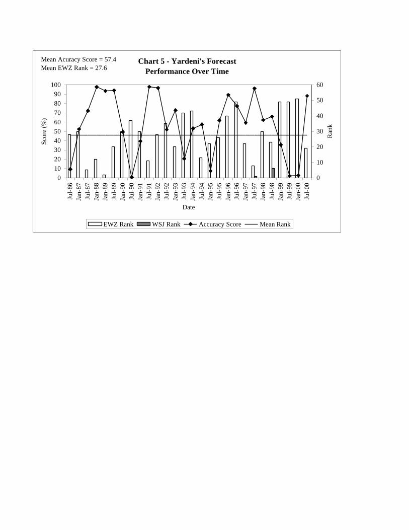
Chart 5 - Yardeni's Forecast Performance Over Time

0102030405060708090

100

Jul-

86Ja

n-87

Jul-

87Ja

n-88

Jan-

89Ju

l-89

Jan-

90Ju

l-90

Jan-

91Ju

l-91

Jan-

92Ju

l-92

Jan-

93Ju

l-93

Jan-

94Ju

l-94

Jan-

95Ju

l-95

Jan-

96Ju

l-96

Jan-

97Ju

l-97

Jan-

98Ju

l-98

Jan-

99Ju

l-99

Jan-

00Ju

l-00

Date

Scor

e (%

)

0

10

20

30

40

50

60

Ran

k

EWZ Rank WSJ Rank Accuracy Score Mean Rank

Mean Acuracy Score = 57.4Mean EWZ Rank = 27.6

Table 1 - Forecast Performance for Top Forecasters July 1999 WSJ Survey

3-Month T-Bill Rate

GDP Growth

Rate CPI

Inflation

Civilian Unemployment

Rate

30-Year T-Bond

Rate

Yen/Dollar Exchange

Rate EWZ Rank Accuracy

Score WSJ Rank Cahn 4.90 3.63 2.4 4.0 6.50 120 7 73.84 4

Dudley 5.00 3.27 2.5 4.0 5.80 115 4 86.85 6 Fosler 5.25 3.73 2.3 4.0 6.40 110 1 99.64 1

Littmann 4.75 3.27 2.7 4.2 6.15 116 3 87.43 7 Orr 5.45 3.80 2.5 4.2 6.35 135 44 12.73 5

Ramirez 5.40 3.67 2.5 4.0 7.00 125 19 52.31 3 Reynolds 5.20 2.57 2.8 4.7 6.40 117 5 80.29 20

Sinai 5.23 3.13 2.5 4.1 6.55 110 2 99.40 2 Thayer 4.40 2.80 2.2 4.4 5.20 112 6 79.08 37

Actual data 5.32 3.70 2.6 4.1 6.48 102

3-Month T-Bill 1.00 0.14 -0.11 -0.32 0.51 0.48 GDP Growth 0.14 1.00 0.02 -0.34 0.09 0.00

CPI -0.11 0.02 1.00 0.03 0.14 -0.22 Unemployment -0.32 -0.34 0.03 1.00 -0.18 0.01 30-Year T Bond 0.51 0.09 0.14 -0.18 1.00 0.27

Yen/Dollar 0.48 0.00 -0.22 0.01 0.27 1.00

Table 2 - July 1999 WSJ Survey Variance-Covariance Matrix

3-Month

T-Bill Rate GDP

Growth Rate CPI

Inflation


Rate 30-Year

T-Bond Rate

Yen/Dollar Exchange

Rate 3-Month T-Bill 3.27 0.35 -0.18 -0.36 0.87 10.26 GDP Growth 0.35 1.98 0.03 -0.29 0.12 -0.04

CPI -0.18 0.03 0.84 0.02 0.13 -2.44 Unemployment -0.36 -0.29 0.02 0.39 -0.11 0.06 30-Year T Bond 0.87 0.12 0.13 -0.11 0.91 3.09

Yen/Dollar 10.26 -0.04 -2.44 0.06 3.09 140.16 Correlation

3-Month T-Bill Rate

GDP

Growth Rate

CPI

Inflation


Rate

30-Year

T-Bond Rate

Yen/Dollar Exchange

Rate

Standard Standard Number of Jan 2002 Jan 2002Periods Average Deviation Average Deviation Forecast Survey Survey

Forecasters Covered Score of Scores Rank of Ranks Surveys Score Rank

Kudlow**July 88 - Jan 92, Jan 94, Jan

01 - Jan 02 69.6 38.78 19.75 16.42 12 11.4 53Resler Jan 86 - Jan 02 68.3 28.28 18.15 12.17 33 86.9 3

Soss*Jan 88 - Jan 94, July 01 - Jan

02 68.2 26.74 23.21 15.20 14 66.1 15DiClemente July 00 - Jan 02 67.4 44.60 14.25 19.81 4 76.3 9

Hoffman Jan 88 - Jan 02 66.5 26.72 19.89 9.44 28 33.5 38Levy Jan 86- Jan 02 63.7 29.38 22.18 10.79 33 33.5 37

WyssJan 89 - July 99, July 01 - Jan

02 63.6 27.86 25.48 12.95 29 60.3 20Harris July 86 - Jan 02 62.8 31.35 21.68 12.59 31 42.7 30

Hymans July 86 - Jan 02 62.3 32.81 21.34 14.20 29 80.8 6Swonk July 98 - Jan 02 61.7 29.30 19.57 16.97 7 71.9 12

Littmann Jan 93- Jan 02 61.5 32.34 22.72 14.83 18 82.8 5Perna July 94 - Jan 02 61.4 31.33 21.25 14.48 16 37.4 34Sinai Jan 86 - Jan 02 61.0 32.15 25.29 15.52 31 1.9 55

Berson Jan 90-Jan 02 60.7 28.88 22.52 13.24 25 26.1 43Rippe Jan 90 - Jan 02 60.7 31.22 24.28 11.23 25 76.8 8Daane July 88 - Jan 02 60.5 30.32 24.33 14.33 27 20.6 49

Karl Jan 94 - Jan 02 60.5 31.63 24.25 13.74 16 46.6 26Hyman/Lazar Jan 86 - Jan 02 59.7 28.46 25.68 12.13 31 72.4 11

Cosgrov e Jan 94 - Jan 02 59.7 32.99 25.65 16.48 17 62.9 19Ramirez July 92 - Jan 02 59.4 28.85 26.58 16.48 19 68.8 14Sy nnott July 94 - Jan 02 59.4 31.34 22.13 16.80 16 69.8 13

Berner/Greenlaw Jan 94-Jan 02 59.2 31.59 28.09 18.23 17 65.6 16Wilson Jan 86, Jan 01 - Jan 02 58.4 30.67 16.25 14.29 4 29.6 41Sterne July 94, July 99 - Jan 02 57.4 29.93 22.00 13.35 9 89.0 2Muell er July 91- Jan 02 56.3 31.30 26.68 14.94 19 49.1 25

McCulley July 94- Jan 02 55.0 30.93 25.87 13.23 15 49.4 24Coons Jan 94 - Jan 02 54.9 31.12 26.65 15.45 17 40.5 32

Hummer Jan 93 - Jan 02 54.7 28.61 28.37 12.12 19 65.5 17Thay er July 99 - Jan 02 54.3 21.83 21.17 15.05 6 21.5 47Lonski Jan 94- Jan 02 53.9 31.81 27.82 15.40 17 56.2 22Zandi July 95 - Jan 02 52.9 26.06 30.10 11.83 13 52.7 23

Dudley Jan 96 - Jan 02 51.7 37.99 32.38 19.16 13 65.5 18Sohn Jan 98 - Jan 02 51.4 32.25 24.89 17.25 9 12.6 52Smith Jan 87 - Jan 02 49.0 35.65 32.72 17.38 29 26.0 44

Herrick July 94 - Jan 02 48.4 30.74 32.94 15.19 16 39.3 33Shepherdson July 99 - Jan 02 47.4 28.87 25.50 19.17 6 25.5 45Laufenberg July 95 - Jan 02 47.0 35.45 29.57 20.68 14 92.3 1

Fosler Jan 91 - Jan 02 45.6 34.17 32.57 19.64 23 32.7 39Steinberg July 97 - Jan 02 45.6 29.66 29.40 14.99 10 45.7 27

Ev ans Jan 94 - July 96 45.5 32.88 33.71 17.50 7 18.3 50Gallagher Jan 99 - Jan 02 45.1 28.92 33.43 12.50 7 15.1 51

Ally n July 93-Jan 02 44.3 31.77 34.24 12.53 17 36.7 35Orr July 99 - Jan 02 40.0 36.90 31.00 15.85 6 40.8 31

Camilli July 99 - Jan 02 39.9 37.80 29.17 16.94 6 44.5 29Yamarone July 99 - Jan 02 39.8 33.62 29.33 18.82 6 21.5 48

Shilling Jan 86 - Jan 02 39.7 33.71 32.90 16.94 31 3.7 54Wesbury July 98 - Jan 02 35.9 33.35 33.02 20.18 7 30.2 40

* Soss's record was accumulated over largely the late1980s and early 1990's. His rank in July 2001 was 51st.** Kudlow's record was accumulated ov er largely the late 1980s and early 1990s. His ranks in Jan. and July of 2001 were 41st and 5th, respectiv ely .

Overall Forecast Performance For Those Forecasters With Four or More AvailableForecasts

Table 3

Standard Standard Number ofPeriods Average Deviation Average Deviation Forecast

Forecasters Covered Score of Scores Rank of Ranks SurveysMcDevitt July 96- July 01 59.0 29.93 26.89 13.99 9Angell July 94-July 01 58.8 34.99 23.67 16.25 15

Englund Jan 94 - July 01 46.2 26.24 33.27 13.87 15Cahn July 95 - Jan 01 59.2 29.12 27.40 14.01 10Blitzer July 94-Jan 01 55.8 30.05 27.64 17.82 14

Bussman July 97 - Jan 01 44.7 29.83 32.83 8.47 6Moskow itz Jan 86- July 99, July 00 65.2 29.45 19.79 10.53 28

Brown Jan 92 - July 00 59.6 33.12 27.39 17.80 18Yardeni July 87 - July 00 57.0 30.35 27.25 15.05 28Walter Jan 97 - July 00 54.9 35.58 27.75 22.77 8Platt July 88 - Jan 00 68.7 28.00 21.26 13.20 23

Reynolds July 86 - Jan 00 65.0 29.56 24.59 14.42 27Braverman Jan 86 -Jan 99 71.6 27.31 20.00 13.88 28Worseck Jan 89 - Jan 99 62.6 36.24 24.11 18.64 19Williams Jan 94 - Jan 99 56.4 31.40 28.09 12.77 10Karczmar July 93 - July 98 47.7 32.38 36.00 14.82 10

Boltz Jan 86 -Jan 98 62.0 30.27 25.24 15.59 25Leisenring July 87- July 97 73.7 22.95 19.52 11.69 21Bostian Jan 94 -July 97 64.4 29.24 23.63 17.11 8Palash July 95 - July 97 60.5 20.52 34.80 19.06 5

Straszheim July 86 - Jan 97 70.7 26.55 16.05 10.30 21Kellner Jan 86 - Jan 97 62.7 33.24 24.14 13.55 22

Dederick July 86 - July 96 72.1 29.66 18.62 12.13 21Laughlin July 94- July 96 58.6 28.05 24.20 15.94 5Evans Jan 94 - July 96 50.0 33.43 31.00 17.48 6Reaser July 92 - Jan 96 72.8 25.62 15.50 8.42 8

Robertson Jan 86 - Jan 96 69.4 30.73 17.45 10.36 20Wahed July 89 - Jan 96 65.4 34.91 22.42 12.92 12Kahan Jan 87 - Jan 96 62.0 35.20 22.24 15.11 17Keran Jan 94- Jan 96 51.3 21.19 27.40 17.99 5

Ciminero Jan 94, Jan 95 - Jan 96 48.2 37.25 25.50 14.71 4Gramley Jan 87-Jan 95 72.5 31.33 16.00 11.29 17Vignola July 92 - July 94 66.9 32.02 24.20 15.61 5Barbera Jan 90-Jan 94 56.2 32.56 29.11 8.65 9Hoey Jan 86 - Jan 94 54.0 33.66 25.00 11.58 16

Eickhoff July 91 - July 93 93.2 10.73 10.20 11.65 5Lerner July 86- July 93 62.5 26.52 23.73 13.12 15Jones July 86 - Jan 93 71.1 28.72 17.47 9.01 15Melton Jan 86- Jan 93 64.7 33.49 20.87 10.64 15

Michaelis July 87- Jan 92 78.4 28.54 11.50 7.44 10Jordan Jan 89 - Jan 92 56.6 39.35 21.00 12.37 7Schott Jan 86 - Jan 91 76.6 26.49 10.00 5.55 11Cooper Jan 86 - July 90 69.2 32.01 12.10 9.30 10Pate Jan 87 - July 89 82.3 25.67 11.33 9.42 6

Nathan July 96- Jan 89 64.6 30.55 19.50 6.72 6Hunt Jan 86 - Jan 89 41.5 31.12 26.43 6.70 7

Maude July 86- July 88 65.5 26.48 22.00 8.34 5How ard Jan 86 - July 87 40.7 35.96 21.25 8.46 4

Table 3 (cont.)

Overall Forecast Performance For Those Forecasters With Four or MoreAvailable Forecasts

Evaluating Wall Street Journal Survey Forecasters

Documents

Transcript of Evaluating Wall Street Journal Survey Forecasters