Disagreement Among Forecasters in G7 Countries
70
WORKING PAPER SERIES NO 1082 / AUGUST 2009 DISAGREEMENT AMONG FORECASTERS IN G7 COUNTRIES by Jonas Dovern, Ulrich Fritsche and Jiri Slacalek
-
Upload
uni-hamburg -
Category
Documents
-
view
0 -
download
0
Transcript of Disagreement Among Forecasters in G7 Countries
Work ing PaPer Ser i e Sno 1082 / auguSt 2009
DiSagreement among forecaSterS in g7 countrieS
by Jonas Dovern, Ulrich Fritsche and Jiri Slacalek

WORKING PAPER SER IESNO 1082 / AUGUST 2009
This paper can be downloaded without charge fromhttp://www.ecb.europa.eu or from the Social Science Research Network
electronic library at http://ssrn.com/abstract_id=1456859.
In 2009 all ECB publications
feature a motif taken from the
€200 banknote.
DISAGREEMENT AMONG
FORECASTERS IN G7 COUNTRIES 1
by Jonas Dovern 2, Ulrich Fritsche 3
and Jiri Slacalek 4
1 We are grateful to Torsten Schünemann and David Sondermann for excellent research assistance; to Jonathan Wright for helpful comments and
programs to estimate the UCSV model; to Michael Ehrmann, Michael Lamla, Bartosz Maćkowiak, Adina Popescu and seminar audiences at the
Česká národní banka, ECB and ZEW Mannheim for valuable feedback; and to Philip Hubbard for information about the data. Online appendix
with additional results and replication programs are available at http://www.slacalek.com/research/dfs09disagreement/dfs09disagreement_
onlineAppendix.pdf and http://www.slacalek.com/research/dfs09disagreement/dfs09disagreement.zip respectively.
The views presented in this paper are the authors’, and do not necessarily reflect those of the European Central Bank.
2 Kiel Economics Research & Forecasting, Fraunhoferstr. 13, D-24118 Kiel, Germany; e-mail: [email protected]
3 University of Hamburg, Edmund-Siemers-Allee 1, D-20146 Hamburg, Germany; e-mail: [email protected];
http://www.ulrich-fritsche.net/
4 European Central Bank, Kaiserstrasse 29, D-60311 Frankfurt am Main, Germany; e-mail: [email protected];
http://www.slacalek.com/
© European Central Bank, 2009
Address Kaiserstrasse 29 60311 Frankfurt am Main, Germany
Postal address Postfach 16 03 19 60066 Frankfurt am Main, Germany
Telephone +49 69 1344 0
Website http://www.ecb.europa.eu
Fax +49 69 1344 6000
All rights reserved.
Any reproduction, publication and reprint in the form of a different publication, whether printed or produced electronically, in whole or in part, is permitted only with the explicit written authorisation of the ECB or the author(s).
The views expressed in this paper do not necessarily refl ect those of the European Central Bank.
The statement of purpose for the ECB Working Paper Series is available from the ECB website, http://www.ecb.europa.eu/pub/scientific/wps/date/html/index.en.html
ISSN 1725-2806 (online)
3ECB
Working Paper Series No 1082August 2009
Abstract 4
Non-technical summary 5
1 Introduction 7
2 The data 10
2.1 The data set 10
2.2 Fixed event and fi xed horizon forecasts 11
2.3 Descriptive statistics 12
3 Drivers of disagreement 14
3.1 A fi rst look at disagreement 14
3.2 Disagreement over time 15
3.3 An intermezzo on macroeconomic volatility 16
3.4 Disagreement and macro variables 18
3.5 Disagreement andcentral bank independence 19
4 Disagreement across countries 21
4.1 Country-by-country regression analysis 21
4.2 Cross-variable and cross-country linksbetween disagreement 22
5 Turbulent expectations 2008-2009 23
6 Conclusion 24
References 24
Tables and fi gures 28
European Central Bank Working Paper Series 67
CONTENTS
4ECBWorking Paper Series No 1082August 2009
Abstract. Using the Consensus Economics dataset with individual expertforecasts from G7 countries we investigate determinants of disagreement (cross-sectional dispersion of forecasts) about six key economic indicators. Disagree-ment about real variables (GDP, consumption, investment and unemploy-ment) has a distinct dynamic from disagreement about nominal variables(inflation and interest rate). Disagreement about real variables intensifiesstrongly during recessions, including the current one (by about 40 percent interms of the interquartile range). Disagreement about nominal variables riseswith their level, has fallen after 1998 or so (by 30 percent), and is consider-ably lower under independent central banks (by 35 percent). Cross-sectionaldispersion for both groups increases with uncertainty about the underlyingactual indicators, though to a lesser extent for nominal series. Country-by-country regressions for inflation and interest rates reveal that both thelevel of disagreement and its sensitivity to macroeconomic variables tend tobe larger in Italy, Japan and the United Kingdom, where central banks be-came independent only around the mid-1990s. These findings suggest thatmore credible monetary policy can substantially contribute to anchoring ofexpectations about nominal variables; its effects on disagreement about realvariables are moderate.
Keywords: disagreement, survey expectations, monetary policy, forecasting
JEL Classification: E31, E32, E37, E52, C53
5ECB
Working Paper Series No 1082August 2009
Non-technical Summary
Macroeconomic models often impose homogeneity. Agents have the samepreferences, beliefs, information sets, are hit with the same shocks or processinformation in the same way. Such assumptions are convenient because theymake models simple and tractable while keeping them useful for aggregate policyanalysis. However, evidence from micro data and casual observations show thatpeople differ from each other, and economists have recently put much effort intoconstructing and studying models that can account for some of the differences.
Expectations are known to be a crucial determinant of economic dynamics.Although existing micro datasets make it possible to measure and test manyaspects of heterogeneity (e.g., differences in income, portfolios, demographics,shocks or labor force status), they typically contain little information aboutexpectations. In addition, even when such information exists, the length andfrequency of the series do not allow to adequately investigate how the cross-sectional distribution of expectations varies over time, business cycle and witheconomic policy. Consequently, there has been little work on joint analysis ofindividual survey expectations across countries and variables with micro data.
We investigate determinants of disagreement (cross-sectional dispersion offorecasts) about six key economic indicators in G7 countries roughly over thepast twenty years. Using a unique dataset with individual expert forecasts fromConsensus Economics we provide a set of statistics that capture the key featuresof dynamics of disagreement and are consistently calculated across countries andvariables. The dataset has been used quite extensively (see references below) butmost work investigates the central tendency—consensus—not the cross-sectionaldistribution of forecasts. Although it is often challenging in large datasets likeours, which covers six variables in seven countries, to find consistent results, tosummarize them and interpret, a number of results emerge quite clearly fromour analysis.
We find that disagreement about real variables (GDP, consumption, invest-ment and unemployment) has a distinct dynamic from disagreement about nom-inal variables (inflation and interest rate). Disagreement about real variablesintensifies strongly during recessions (by about 40 percent in terms of the in-terquartile range). Disagreement about nominal variables rises with their level,has fallen after 1998 or so (by 30 percent), and is considerably lower under inde-pendent central banks (by 35 percent). For both groups cross-sectional disper-sion increases with uncertainty about the underlying actual indicators, thoughto a lesser extent for nominal series, and disagreement is more strongly cross-correlated among variables within the groups than between them.
While we provide simple and transparent reduced-form estimates, we believeour statistics also suggest a causal relationship: central bank independence re-duces disagreement about nominal variables. Country-by-country regressionsfor inflation and interest rates reveal that both the level of disagreement andits sensitivity to macroeconomic variables tend to be larger in Italy, Japan andthe United Kingdom, where central banks became independent only around themid-1990s. These findings suggest that more credible monetary policy can sub-stantially contribute to anchoring of expectations about nominal variables. Incontrast, its effects on disagreement about real variables are moderate.
6ECBWorking Paper Series No 1082August 2009
While our analysis uses data on expectations of professional forecasters, qual-itatively similar results may obtain also for other economists (in industry, gov-ernment and academia) and households. This could be the case if our data aretaken as a proxy for expectations of the rest of population, or if news spreadepidemiologically from experts to other agents.
We believe our results could be of interest to both policy-makers and re-searchers. The large literature on monetary theory and policy agrees that an-chored inflation expectations are of utter importance for safeguarding of pricestability. Much work has documented that the inflation and GDP processes inG7 countries moderated in the late 1980s and their volatility has been fallingfurther most of the time until recently. Our dataset confirms the existing find-ings that the consensus (mean) expectations have also stabilized for most coun-tries and variables. However, for expectations to be perfectly anchored it isnecessary that also their cross-sectional dispersion—disagreement—disappears.Our results document across several countries and variables the extent to whichthis has been the case and suggest how economic shocks and monetary pol-icy setting contributed to the reduction of disagreement we often find in the2000s. Researchers could use the stylized facts we report to calibrate, test andimprove models with heterogeneous beliefs, learning or information processingconstraints, which have recently become quite widespread.
7ECB
Working Paper Series No 1082August 2009
1. Introduction
Macroeconomic models often impose homogeneity. Agents have the samepreferences, beliefs, information sets, are hit with the same shocks or processinformation in the same way. Such assumptions are convenient because theymake models simple and tractable while keeping them useful for aggregate policyanalysis. However, evidence from micro data and casual observations show thatpeople differ from each other, and economists have recently put much effort intoconstructing and studying models that can account for some of the differences.1
Expectations are known to be a crucial determinant of economic dynamics.2
Although existing micro data sets make it possible to measure and test manyaspects of heterogeneity (e.g., differences in income, portfolios, demographics,shocks or labor force status), they typically contain little information aboutexpectations. In addition, even when such information exists, the length andfrequency of the series do not allow to adequately investigate how the cross-sectional distribution of expectations varies over time, business cycle and witheconomic policy. Consequently, there has been little work on joint analysis ofindividual survey expectations across countries and variables.
We investigate determinants of disagreement (cross-sectional dispersion offorecasts) about six key economic indicators in G7 countries roughly over thepast twenty years. Using a unique data set with individual expert forecasts fromConsensus Economics we provide a set of statistics that capture the key featuresof dynamics of disagreement and are consistently calculated across countries andvariables. The data set has been used quite extensively (see references below) butmost work investigates the central tendency—consensus—not the cross-sectionaldistribution of forecasts. Although it is often challenging in large data sets likeours, which covers six variables in seven countries, to find consistent results, tosummarize them and interpret, a number of results emerge quite clearly fromour analysis.
We find that disagreement about real variables (GDP, consumption, invest-ment and unemployment) has a distinct dynamic from disagreement about nom-inal variables (inflation and interest rate). Disagreement about real variablesintensifies strongly during recessions (by about 40 percent in terms of the in-terquartile range). Disagreement about nominal variables rises with their level,has fallen after 1998 or so (by 30 percent), and is considerably lower under inde-pendent central banks (by 35 percent). For both groups cross-sectional disper-sion increases with uncertainty about the underlying actual indicators, though
1For example, models in which some households are more impatient than others (or are sub-ject to liquidity constraints) are useful in studying the monetary policy transmission mechanism(Iacoviello, 2005). Models with heterogeneous beliefs/expectations are becoming popular in as-set pricing literature (see Scheinkman and Xiong, 2003 for a survey). Carroll (1997) and Kruselland Smith (1998) model reaction of agents’ consumption–saving behavior to idiosyncratic (andaggregate) income shocks. Morris and Shin (2005b) investigate the value of providing of publicinformation to agents depending on the amount of private information they have.
2See Bernanke (2004), Morris and Shin (2005a), Woodford (2005) and many others.
8ECBWorking Paper Series No 1082August 2009
to a lesser extent for nominal series, and disagreement is more strongly cross-correlated among variables within the groups than between them.
While we provide simple and transparent reduced-form estimates, we believeour statistics also suggest a causal relationship: central bank independence re-duces disagreement about nominal variables. Country-by-country regressionsfor inflation and interest rates reveal that both the level of disagreement andits sensitivity to macroeconomic variables tend to be larger in Italy, Japan andthe United Kingdom, where central banks became independent only around themid-1990s. These findings suggest that more credible monetary policy can sub-stantially contribute to anchoring of expectations about nominal variables. Incontrast, its effects on disagreement about real variables are moderate.
We believe our results could be of interest to both policy-makers and re-searchers. The large literature on monetary theory and policy agrees that an-chored inflation expectations are of utter importance for safeguarding of pricestability. Much work (including Cogley and Sargent, 2001; Stock and Watson,2002 and Stock and Watson, 2005) has documented that the inflation and GDPprocesses in G7 countries moderated in the late 1980s and their volatility hasbeen falling further most of the time until recently.3 Our data set confirms theexisting findings that the consensus (mean) expectations have also stabilized formost countries and variables. However, for expectations to be perfectly anchoredit is necessary (though not sufficient) that also their cross-sectional dispersion—disagreement—disappears. Our results document across several countries andvariables the extent to which this has been the case and suggest how economicshocks and monetary policy setting contributed to the reduction of disagreementwe often find in the 2000s. Researchers could use the stylized facts we report tocalibrate, test and improve models with heterogeneous beliefs, learning or infor-mation processing constraints, which have recently become quite widespread.4
Our work builds on two strands of literature on survey expectations. The firstand larger area analyzes the central tendency in expectations about inflation,GDP, interest rates and exchange rates.5 The second, more recent and more
3More precisely, the work typically finds that the variance of the permanent component ofinflation and GDP was declining before 2006 or so. In addition, evidence below documents thatthe average variance of the permanent component of the six series we investigate was typicallyhigher in the 1990s than in the 2000s.
4For example, Erceg and Levin (2003) use the consensus inflation expectations from theUS Survey of Professional Forecasters to calibrate the signal-to-noise ratio, which determineshow households and firms disentangle persistent shifts in inflation target from transitory dis-turbances in the monetary policy rule. The ratio is the key determinant of the persistence ofactual inflation and output. Mankiw, Reis, and Wolfers (2003) compare how the sticky infor-mation model matches cross-sectional dispersion of inflation forecasts in various US surveys.Bloom, Floetotto, and Jaimovich (2009) document that uncertainty about economic activity isstrongly counter-cyclical and build a dynamic stochastic general equilibrium model with het-erogeneous firms, non-convex adjustment costs and changing variance of productivity shocks.In such model a rise in uncertainty leads to a fall in output.
5For example, Branch (2004) estimates a model of boundedly rational agents on inflation ex-pectations from the Survey of Consumer Attitudes and Behavior of the University of Michigan.Ang, Bekaert, and Wei (2007) find that survey expectations provide better inflation forecasts
9ECB
Working Paper Series No 1082August 2009
closely related body of work investigates heterogeneity in expectations, oftenusing micro data. The key inspiration for our work is a recent important paperof Mankiw et al. (2003), which analyzes central tendency and dispersion of in-flation expectations using several US survey data sets, and tests some theoriesof disagreement. Separate work of Souleles (2004) uses the Michigan Survey ofConsumer Attitudes and Behavior to examine the ability of various groups ofpopulation to forecast consumption expenditure. Blanchflower and Kelly (2008)study determinants of inflation expectations in the Bank of England’s InflationAttitudes Survey and the European Commission’s consumer survey. Pattonand Timmermann (2008b) use a simple reduced-form state-space model to ex-plain the cross-sectional dispersion of US GDP growth and inflation forecastsand argue that forecasters’ heterogeneity in prior beliefs is more important thanheterogeneity in information sets. Lahiri and Sheng (2009) show, using a decom-position of forecasts errors into common and idiosyncratic shocks, that aggregateforecast uncertainty can be expressed as a combination of disagreement amongthe forecasters and the perceived variability of future aggregate shocks. Carroll(2003) bridges the two strands of literature by proposing and testing a modelof average inflation and unemployment expectations of households interact withthose of experts. But joint analysis of individual survey expectations acrosscountries and variables is so far under-researched.
The estimates below capture dynamic correlations, conditional on the explana-tory variables included in the regressions. Besides being potentially subject tostandard econometric issues, such as mis-specification or omitted-variable bias,our estimates can to some extent be affected by endogeneity and, as a result,caution is required to draw strong conclusions about the causal nature of the es-timated relationships. We have undertaken a large number of robustness checks(some of which are in the online appendix). We believe the results reported inthis paper are reasonably stable although it is of course likely that future workon the topic will provide new, more refined insights.
than macro variables or asset markets. Bernanke and Boivin (2003) and Faust and Wright(2007) compare the Greenbook inflation and GDP forecasts (produced by the US Federal Re-serve) to predictions generated by reduced-form econometric models. Kim and Orphanides(2005), Piazzesi and Schneider (2008) and others use interest rate expectations from the USSurvey of Professional Forecasters to improve on the existing yield curve models.
Much work, like us, uses the Consensus Economics data set, although often just the centraltendency rather than the whole cross-section of observations. For example, Engel and Rogers(2008) and Devereux, Smith, and Yetman (2009) use expectations of consumption, inflationand exchange rates to test models of international risk sharing. Engel, Mark, and West (2008)feed inflation forecasts into the present-value model of the exchange rate in order to evaluateits forecasting performance. Levin, Natalucci, and Piger (2004) investigate the degree to whichinflation expectations are anchored in industrial countries. Patton and Timmermann (2008a)study how uncertainty about macroeconomic variables is resolved using forecasts of US inflationand GDP growth.
Separate large literature exists on extracting inflation expectations from prices of indexedbonds. For example Gurkaynak, Levin, and Swanson (2006), Ehrmann, Fratzscher, Gurkaynak,and Swanson (2007) and Beechey, Johannsen, and Levin (2008) use high-frequency financialdata to provide evidence complementary to ours on anchoring of long-run inflation expectationsin the euro area, Sweden, the UK and the US.
10ECBWorking Paper Series No 1082August 2009
2. The Data
2.1. The Data Set. We use a leading cross-country survey data set compiledby Consensus Economics, http://www.consensuseconomics.com/, a London-based economic survey organization.6 Each month, starting in October 1989,Consensus Economics polls experts from public and private economic institu-tions, mostly investment banks and economic research institutes, about theirpredictions about the most common macroeconomic indicators. Neither centralbanks nor governments participate in the survey. Our sample ranges betweenOctober 1989 and October 2006 and consists of 205 monthly observations.
While the survey is now conducted in more than twenty countries, the largestsample in terms of length and cross-sectional dimension (number of respondents)is available for G7 countries.7 Essentially the same survey is conducted in all G7countries using the same procedure: forecasters fill out the survey form mostlyelectronically in the first two weeks of each month and the data are publishedaround the middle of the month. In addition, country-specific expertise is guar-anteed as most panelists are located in the country they are analyzing. Conse-quently, the data set is comparable both across countries and across panelists,and collects some of the best economic forecasts.
The data set covers all principal macroeconomic indicators. We focus on thefollowing six: consumer-price inflation, nominal three-month interest rate, GDPgrowth, consumption growth, investment growth and unemployment rate.8 Al-though the survey contains information on other variables (most importantly,industrial/manufacturing production, producer prices, wages, current accountand budget balance), their coverage in terms of time period, countries and num-ber of respondents is less complete. These additional indicators are also arguablyless important and often less closely followed by forecasters than those we focuson.
Before the analysis we cleaned and transformed the data as follows. Thestarting point are the expectations series as given in the reports of ConsensusEconomics. We are able to keep track of the series of each forecaster and at-tempt to follow them as their institutions merged with others, were taken overor renamed (see the the online appendix). We checked the individual expecta-tions, which substantially differ from others (e.g., three inflation expectations in
6Several other data sets of economic forecasts of experts exist both in the US (Survey ofProfessional Forecasters and the Livingston Survey) and in Europe (European Central Bank’sSurvey of Professional Forecasters). These surveys typically cover only a single country oreconomic region (euro area), a subset of variables (most prominently inflation), or a shortertime period than the Consensus Economics survey.
7Although the survey currently covers all major industrial countries and many emergingeconomies, data from some relatively large European countries (such as Spain, the Netherlandsor Sweden) have only been available since December 1994. Expectations about the euro areavariables only go back to December 2002 (and are subject to composition effects as new countriesjoined the monetary union).
8We have also investigated expectations about industrial production but only report theseresults, which are broadly consistent with those for GDP in the online appendix.
11ECB
Working Paper Series No 1082August 2009
Japan in February and March 2002) and made sure they correctly reflect thefigures in the reports.9 For each respondent some observations—typically about10 percent—were linearly interpolated when a single observation was missing(and both adjacent observations were available) within a year or when two ob-servations were missing at the beginning or at the end of the year.
2.2. Fixed Event and Fixed Horizon Forecasts. Except for interest rates,the respondents give their expectations over the current and the next calendaryear; the survey data thus provides series of fixed event forecasts.10 However, webelieve fixed horizon (e.g., one-year-ahead) forecasts are preferable for the anal-ysis of disagreement because forecasting horizon of fixed event forecasts variesfrom month to month and consequently their uncertainty and cross-sectionaldispersion is strongly seasonal. In addition, we use fixed horizon forecasts be-cause we want to provide comparable results to much of the literature, includingMankiw et al., 2003.
We approximate fixed horizon forecasts as a weighted average of fixed eventforecasts as follows. Denote F fe
y0,m,y1(x) the fixed event forecast of variable x foryear y1 made in month m of previous year, y0 = y1−1, and F fh
y0,m,12(x) the fixedhorizon, twelve-month-ahead forecast made at the same time. For example, theNovember 2008 forecast for year 2009 is F fe
2008,11,2009(x). We approximate thefixed horizon forecast for the next twelve months as an average of the forecastsfor the current and next calendar year weighted by their share in forecastinghorizon:
F fhy0,m,12(x) =
12−m + 112
F fey0,m,y0(x) +
m− 112
F fey0,m,y0+1(x). (1)
For example, the November 2008 forecast of inflation rate between November2008 and November 2009 is approximated by the sum of F fe
2008,11,2008(π) andF fe
2008,11,2009(π) weighted by 212 and 10
12 respectively.We use this procedure for the five variables with the exception of interest rate,
which is reported as the fixed-horizon forecast of interest rate between now andthree months from now.
Because the disagreement series is used only as the dependent variable, theapproximation/measurement error in series F fh
y0,m,12(x) from (1) does not affectthe consistency of the regression estimates obtained below as long as the erroris not correlated with regressors. Such correlation should be relatively low alsogiven the high, monthly frequency of the data.
It is ultimately an empirical question how well our approximation performs.Using fixed event and fixed horizon forecasts in the US Survey of Professional
9It is possible that these outliers could have been due to typing errors by respondents.However, our measure of disagreement—the cross-sectional interquartile range—is robust tothe presence of a limited number of outliers.
10Once every quarter the survey includes additional questions for selected variables (CPIinflation, GDP, consumption) on the fixed horizon predictions for roughly the following twoyears. However, these questions are not useful for the analysis of disagreement because onlythe consensus (mean) forecasts are published.
12ECBWorking Paper Series No 1082August 2009
Forecasters, Dovern and Fritsche (2008) find that approach (1) captures wellcross-sectional dispersion of predictions. Correlation between cross-sectional dis-persion in (1) and the true dispersion of fixed horizon forecasts is roughly 0.8–0.9when measured with standard deviation and 0.6–0.9 for the interquartile range(IQR). The remaining nine methods Dovern and Fritsche investigate, includ-ing several specifications with unobserved components and seasonal adjustment,typically correlate with the true dispersion at 0.5–0.9 for standard deviation and0.2–0.8 for the interquartile range.
As the final issue, we need to decide about our preferred measure of cross-sectional dispersion of forecasts. Throughout the paper we use the width of theinterquartile range, the difference between the third and first quartile of obser-vations. We do so to be consistent with the previous work (Mankiw et al., 2003)and because the IQR is also likely to be more robust to outliers than standarddeviation. The results for disagreement measured with standard deviation areconsistent with those presented below, which is not surprising given the rela-tively high correlation (0.7–0.8) between the two measures shown in Table 15 inthe Appendix.11
2.3. Descriptive Statistics. Before we analyze disagreement among forecast-ers in more detail, let’s have a closer look at the data. Figures 1–6 comparethe expected and actual variables. The actual series are shifted backward bytwelve months so that the vertical difference between them and expectations isthe expectation error. (For example, for November 2003, the dots denote expec-tations of one-year ahead inflation rate and the actual series is inflation betweenNovember 2003 and November 2004.) The shaded areas denote recessions asidentified by the Economic Cycle Research Institute (using the business cyclemethod, which mirrors the NBER procedure).
Three findings appear for all six expectation series. First, expectations aremore stable than the actual series as the actual series contain substantial unpre-dictable and volatile component.
Second, expectations are sensitive to current conditions: expected one-yearahead rates are quite strongly correlated with the currently observed rates. Thisis perhaps not surprising in case of inflation, interest rate and unemployment,which are generally known to be quite persistent (so that the last observationis a good predictor of the future one(s)). However, the sensitivity to currentconditions is also apparent—although to a lesser extent—for variables like GDPgrowth, which are not highly serially correlated.
Third, expectations are sluggish in that they typically overestimate the de-velopments when the underlying variable is falling. This finding is apparent
11For a normal distribution standard deviation (stdev) is proportional to the interquartilerange, stdev = 1.349× IQR (because the 75th percentile of the standard normal distribution is0.6745). This scaling on average roughly holds in our data, e.g. for inflation in Canada averageIQR = 0.34 and stdev×1.349 = 0.26 × 1.349 = 0.35. The Shapiro–Wilk test does not rejectnormality in cross-section about 85–90 percent of time (somewhat below what is implied by itsnominal size of 0.05).
13ECB
Working Paper Series No 1082August 2009
for example during the disinflations of the early 1990s when inflation expecta-tions errors were on average positive. The result is clearer for more persistentvariables—inflation, interest rates and unemployment—than for those subjectto large transitory fluctuations (GDP, consumption and investment).
Table 1 summarizes the key descriptive statistics about expectations and ac-tual series. Average number of forecasters, displayed in the first line of eachpanel, typically ranges between 15 and 35 and shows little systematic variationover time: while in Canada, Japan and the US it is approximately constant, itrises somewhat in France, Germany and Italy and falls in the UK after 2000 orso. The number of respondents does not correlate with the phase of the businesscycle, and varies little across variables (in a given country). Observations foreach forecaster are available for about half of the time on average.
The second line in each panel shows the mean expectation error averagedacross forecasters and time periods. The individual forecasts are not statisticallysignificantly biased partly because the standard deviation of expectation errorsis quite large. (The bias of consensus, or mean, forecasts is significant for a fewvariables in some countries.) Average expectation errors are typically positive,which may reflect forecasters’ optimism or sluggishness (where the trend in theunderlying variable is falling most of the time, such as in the case of inflationand interest rates).12 There are few systematic differences across countries (forexample, while the US respondents do well in the case of interest rate, they arethe worst in the case of consumption).13
Lines three, four and five give the average mean squared errors of forecasts,average level of the underlying variable and its variance respectively (taken overthe sample period October 1989–October 2006). The level and the varianceof economic variables can plausibly be positively correlated—see Ball and Cec-chetti (1990) and Ball (1992)14 on empirical and theoretical investigation forinflation—and both can positively correlate with the MSEs (and also disagree-ment). However, the evidence in Table 1, based on variables averaged over thesample and summarized in the top panels of Figure 7, implies if anything a neg-ative correlation between the MSE and the level of the underlying variable.15
In contrast, imprecision of expectations tends to increase with the variance ofthe underlying variable, as one would expect. While Figure 7 is subject tomany criticisms—such as that the relationship is only bivariate and based on
12Bias of inflation forecasts tends to quite high and positive before 1999 and negativeafterwards.
13Detailed investigation of bias and efficiency of forecasts is beyond the scope of this paper.Large literature exists on this topic, mostly testing GDP, inflation and unemployment forecasts,including work that uses our data set, e.g. Harvey, Leybourne, and Newbold (2001), Isiklar,Lahiri, and Loungani (2006), Batchelor (2007), and Ager, Kappler, and Osterloh (2009).
14Ball (1992) proposes a model in which the level of inflation and its uncertainty are positivelycorrelated because when inflation is high, policy-makers face a dilemma: they would like todisinflate but fear the resulting recession.
15Note that investment, being an outlier due to large MSEs, is excluded from the Figure tobe able to assess if the positive relationship between the MSE and variance holds even withoutit.
14ECBWorking Paper Series No 1082August 2009
time-averaged statistics—we believe it is an interesting starting point for a morecareful regression analysis of disagreement below.16
3. Drivers of Disagreement
The previous section summarized some key properties of individual expecta-tions. In contrast, this section focuses on the disagreement among forecasters—defined as cross-sectional dispersion and measured with the cross-section in-terquartile range—its evolution over time and its relationship to the businesscycle and monetary policy.
3.1. A First Look at Disagreement. Line six in each panel of Table 1 sum-marizes the average disagreement by country and variable. Full-sample time-average of disagreement about inflation is relatively low for France, Germanyand Italy. Cross-sectional dispersion of interest rates is quite high in Canadaand the US, relatively low in France and Germany, and extremely low in Japan,the last finding being driven by effectively zero interest rates for much of thetime since 2000. Forecasters in France, Germany and Italy agree to a large ex-tent on GDP growth, compared to their counterparts in the UK, Canada andin particular Japan (where the dynamics are again dominated by the recessionpart of the sample). While the series for consumption growth is smoother thanthat for GDP growth, disagreement about consumption tends to be somewhathigher, driven perhaps by less attention that some forecasters pay to the con-sumption series. However, the two disagreement series correlate quite strongly,which one could expect given the large share of consumption in GDP (see alsoFigures 10–11 below for time perspective). Disagreement about investment issubstantially larger than for other series because of its high volatility. Unem-ployment on the other hand is smooth (and predictable), which translates intolittle disagreement.17
Figures 8–13 illustrate the evolution of disagreement over time by country andvariable. Perhaps unsurprisingly given the monthly frequency of our sample, dis-agreement is subject to much transitory but quite persistent variation. However,two findings arise in several countries and series. First, disagreement tends torise during recessions. Second, there is a downward time trend in disagreement.
Disagreement about inflation in Figure 8 is roughly constant in France andGermany but falls steadily after 1992 or so in Italy, as the country was expectedto join the euro area, in Japan and in the UK. The series is quite strongly anti-cyclical (in terms of the difference between its average in recessions and booms)in Canada, Italy, Japan, the UK and the US.
As shown in Figure 9, disagreement about interest rate tends to trend down-ward in all countries except for the US and its dynamics is strongly anti-cyclical
16Because the focus of this paper is on disagreement, we will not investigate the determinantsof MSEs below.
17The somewhat higher mean for Germany is driven by the uncertainty about labor marketstatistics during the re-unification.
15ECB
Working Paper Series No 1082August 2009
(except for Japan where there was little disagreement when the interest rateslied close to zero).
Disagreement about GDP growth in Figure 10 is again anti-cyclical, exceptfor France; in the remaining countries it is typically 30–50% higher in recessionsthan in booms. Disagreement about the remaining real variables (consumption,investment and unemployment) broadly tracks that of GDP.
One can think of at least two structural breaks in our sample: the introductionof the euro in January 1999 and the German re-unification in October 1990. Theexpectations of the first event seem to have affected disagreement about inflationin Italy, which started to fall following the breakdown of the European ExchangeRate Mechanism in September 1992. Disagreement in the remaining two euroarea members, France and Germany, has been roughly constant perhaps becausethe inflation rate in these two countries has been low and stable. Figures 8–13show, the structural break due to the German re-unification in October 1990temporarily elevated disagreement about real variables (GDP, consumption, in-vestment and unemployment), but not about inflation and interest rate. To alarge extent unrelated to these two events, there has been much dynamics indisagreement of various series, in particular the clear downward trend in the UKand cyclical dynamics in most countries. We investigate these developments inmore detail below using simple regression analysis.
3.2. Disagreement over Time. To provide quantitative insights Tables 2–7use the fixed effects panel estimator (in which coefficients other than the constantare restricted to be the same in all countries18) to assess general trends commonin all countries. We discuss the results for the three most important indicators—inflation, interest rates and GDP—in more detail and summarize the remainingvariables (consumption, investment and unemployment) only briefly.
The top panel (Panel A) of each of Tables 2–7 investigates how disagreement(“disagr”) varies over time and during recessions using two versions of regression:
disagrt = β0 + β1 × rect + β2 × post-1998t + ut,
where “rec” denotes the recession dummy and “post-1998” is the dummy for thesecond part of the sample.
Disagreement about inflation is analyzed in Table 2. Row 1 reports that thecross-sectional interquartile range averaged across countries and time is about0.3, which suggests that half of the forecasters typically lie within 0.15 percentagepoints of the consensus. Row 2 shows that disagreement rises by about 15 percentduring recessions, a fact that can be due to the increase in general macroeconomicuncertainty, and that disagreement is much lower—by 25%—in the second partof the sample, after 1998.
Qualitatively similar findings obtain for disagreement about interest rates andGDP growth and are reported in Tables 3 and 4 respectively. For both variables,disagreement rises during recessions and falls after 1998. While the effects for
18The constant term β0 in the Tables is normalized to give the average of country-specificintercepts.
16ECBWorking Paper Series No 1082August 2009
interest rates are quantitatively similar to those for inflation, the increase indisagreement about GDP during recessions is almost twice as large—44 percent(and the fall after 1998 is less pronounced). This seems reasonable as macroeco-nomic uncertainty during a recession is skewed toward GDP (and less evident forinterest rates and, in particular, inflation). The finding is also closely in line withthe evidence in Bloom et al. (2009), who construct a synthetic index of aggregateuncertainty based on measures of cross-firm and cross-industry dispersion, timevariation of aggregate data and forecaster disagreement (about GDP growthand unemployment rate); the index of Bloom et al. indicates that uncertaintyincreases by 42.5 percent during recessions. Results for consumption growth,investment growth and unemployment rate in Tables 5, 6 and 7 respectively areagain qualitatively consistent with the rest.
Qualitatively, the estimates (together with those of Tables 2–3) suggest thatthe recession differential in disagreement—the difference between average dis-agreement in a recession and a boom—is generally larger for real variables (GDP,consumption, investment and unemployment) than for the two nominal vari-ables. In contrast, the fall in disagreement after 1998 tends to be smaller for realvariables than for nominal ones.
Two important broad factors behind the variation in disagreement can bethe shocks to economic variables and economic policy. Larger shocks boost thevolatility of the underlying actual variables and make them less predictable. Asa result, forecasters are more likely to disagree about future outcomes (becauseof using different models, priors, subjective probabilities or data). More credibleeconomic policies can make economic indicators easier to forecast. An obviousexample is the introduction of an explicit numerical inflation target, which cancontribute to better anchoring of inflation expectations. Similarly, independentcentral banks are often perceived as better safeguards to price stability (andcan indirectly also contribute to the stabilization of output). We investigatethese two factors—economic shocks and policies—in a simple reduced-form setupbelow but before doing so we first have to measure them.
3.3. An Intermezzo on Macroeconomic Volatility. To capture the shocksthat hit the underlying actual variable xt we employ the following unobservedcomponent stochastic volatility (UCSV) model of Stock and Watson (2007),which is a simple, canonical device to decompose a series into the permanentand the transitory part with time-varying volatility.19 Intuitively, the dynamicsof xt are driven by a permanent component τt with white noise innovations εt
19The same specification is used in Wright (2008) to model inflation; Stock and Watson(2002) and Stock and Watson (2005) propose variants of this model for GDP, consumption,investment, employment and many other variables. Similar, more sophisticated models areanalyzed in Harvey and Trimbur (2003), Creal, Koopman, and Zivot (2008), Giordani andKohn (2008) and elsewhere.
17ECB
Working Paper Series No 1082August 2009
and a transitory component ηt:
xt = τt + ηt, (2)
τt = τt−1 + εt. (3)
Both ηt and εt are independently normally distributed and have time-varying(random-walk) variances σ2
η,t and σ2ε,t respectively (ηt ∼ N(0, σ2
η,t), εt ∼ N(0, σ2ε,t)):
log σ2η,t = log σ2
η,t−1 + νη,t, (4)
log σ2ε,t = log σ2
ε,t−1 + νε,t. (5)
Innovations to variances νt = (νη,t, νε,t)� are iid N(0, γI2) and γ is a scalarparameter which controls the smoothness of the estimated volatilities σ2·,t. Weestimate the model with the Gibbs sampling.20 We use the UCSV model as aflexible device to capture how the volatility of shocks varies over time. In theregressions below we investigate how disagreement correlates with the varianceσ2
ε,t because permanent uncertainty driven by shocks εt is much more importantfor the formation of expectations (over the next twelve months) than transitoryuncertainty due to ηt, which subsides immediately.21
Figures 14–19 summarize the dynamics of the variance of permanent shocksσ2
ε,t. Full-sample averages of σ2ε,t across countries and variables tend to positively
co-move with those of disagreement. For example, both shocks to investmentand disagreement about it are substantially higher than for other variables. Per-manent shocks to inflation have be quite modest for France, Germany and Italy,and permanent shocks to consumption have generally been larger than those toGDP.
Variance of permanent shocks is also positively related to the path of dis-agreement over time. Forecasters disagree more when the economy is hit withlarger permanent shocks, in particular in recessions but to a lesser extent alsobefore 1999 (compared to the post-1998 period). The key message to take awayfrom the comparison of Figures 8–13 and 14–19 is that both economic shocksand disagreement are more substantial during recessions and tended to be moremuted in the second part of our sample. In addition, the anti-cyclicality of dis-agreement and shocks is somewhat more pronounced for real variables than forinflation.
20The online appendix shows the diagnostics we used to assess the quality of the MCMCapproximation.
21As a robustness exercise we have also proxied uncertainty about the underlying variablext simply with its one-year squared difference Δ12x
2t = (xt − xt−12)
2. An advantage of thatmeasure is that it is independent of the parametric model used to back out σ2
ε,t. For the
specification (2)–(5), Δxt = εt + ηt − ηt−1 and E(Δx2t ) = σ2
ε,t + 2σ2η,t. Estimation results for
this alternative measure of uncertainty (Δ12x2t ) are broadly consistent with the baseline shown
below in sections 3.4 and 3.5. One difference is that disagreement about inflation correlates morestrongly with Δ12INFL2
t than with σ2INFL,ε,t. This is not surprising because both measures of
uncertainty co-move quite closely, with correlation of more than 0.4. (Estimation results andcomparison plots of Δ12x
2t and σ2
x,ε,t are shown in the online appendix.)

18ECBWorking Paper Series No 1082August 2009
3.4. Disagreement and Macro Variables. The middle panel (Panel B) of Ta-bles 2–7 investigates how disagreement correlates with the level of the underlyingactual variables, uncertainty about these variables proxied with the variance ofpermanent shocks, output gap22 and the squared change in the policy interestrate (Δpolicy rate2
t )—a proxy of the variation in monetary policy:
disagrt = β0 + β2 × xt + β3 × σ2x,t + β4 × output gapt + β5 ×Δpolicy rate2
t + ut,
where xt denotes the level of the underlying variable and σ2x,t is a short-hand
notation for the variance σ2x,ε,t of permanent shocks to xt (as given in equation
(5)).Disagreement about inflation rate increases with its level: one percentage
point increase in inflation raises the cross-sectional interquartile range by 0.026,or about 10 percent (with respect to the mean 0.299). The direct effect of in-flation uncertainty (the term σ2
INFL,t), while correctly signed, is statisticallyinsignificant. The coefficient on output gap is negative, which is in line with theprevious evidence that disagreement increases during recessions. Finally, dis-agreement about inflation rises when monetary policy rates change, which againtends to coincide with recessions. (But the positive coefficient on interest ratesis significant even when output gap is included.) In addition, including interestrates among explanatory variables substantially increases the explanatory powerof the regression.
Disagreement about interest rates shown in Table 3 rises with the level, un-certainty and squared change of rates. These findings are in line with the factreported in panel A that disagreement about interest rates fell after 1998, asboth the level and variation in rates is much lower in the second part of the sam-ple (see also Figure 2). In addition, disagreement also tends to move inverselyto the output gap. While the coefficients in these regressions are comparableto those for inflation and GDP growth, their explanatory power is considerablyhigher, and the uncertainty term is significant.
Table 4 analyzes drivers of disagreement about GDP growth. In contrast toinflation and interest rates but in line with the evidence of panel A, disagreementabout GDP growth moves inversely with its level: disagreement rises in periodsof weak economic growth. Arguably, the effects of GDP growth on disagreementare non-linear: disagreement can be expected to rise during periods of heighteneduncertainty, which likely occur during recessions, but also when economic growthaccelerates considerably. (However, the latter periods are virtually absent in oursample as GDP growth only rarely exceeds 5 percent.) In fact, the coefficienton shocks to GDP σ2
GDP,t is estimated to be positive, high and overwhelminglysignificant. As for disagreement about inflation and interest rates, variation ininterest rates analyzed in model 4 also improves the performance of the regression(measured with adjusted R2).
22The output gap used here is the ex post estimate taken from OECD’s Economic Outlook.The series is quarterly, interpolated constant within each quarter, and starts in 1991:Q1.
19ECB
Working Paper Series No 1082August 2009
Given the large share of consumption expenditure on output, it is not sur-prising that the findings for consumption in Table 5 mirror quite closely thosefor GDP. The results are qualitatively similar for investment and unemploymentrate although the explanatory power of investment regressions is smaller (as dis-agreement about investment tends to move more, much of which is unrelated tothe explanatory macro variables).
The results in panel B are also broadly agree with the bivariate illustrationof the relationship between time-averaged disagreement and the level/varianceof the underlying variable in the bottom panels of Figure 7. While the firstcorrelation is close to zero (for reasons outlined above), the one for variance,which proxies better for underlying uncertainty, is positive and quite strong.
Our findings in this and the previous section are in line with Mankiw et al.(2003) and Dopke and Fritsche (2006). Mankiw et al. (2003) report that in theUS disagreement about inflation increases with its level and absolute value ofits change, in particular when the change is sharp, and though it shows anti-cyclical pattern after 1975 or so for consumers, its dependence on the phase ofthe business cycle is less clear for experts. Dopke and Fritsche (2006) find thatdispersion of inflation and growth expectations in Germany is high before andduring recessions and correlates positively with macroeconomic uncertainty.
3.5. Disagreement and Central Bank Independence. It might be a prioriexpected that better macroeconomic policy alleviates economic uncertainty anddisagreement. Without going into much detail about measuring the quality ofeconomic institutions, panel C of Tables 2–7 provides a simple illustration ofhow much better and more credible monetary policy affects disagreement aboutvarious variables. In particular, we attempt to capture credibility of monetarypolicy using an indicator of central bank independence as defined in Table 8.23
We estimate two versions of the following regression
disagrt = β0 + β1 × CB Independencet + β2 × xt + β3 × σ2x,t +
+ β4 × output gapt + β5 ×Δpolicy rate2t + ut.
Although the dummy for central bank independence (CB Independencet) is neg-ative for all variables, it is larger and highly statistically significant for only forinflation, interest rate and unemployment. Quantitatively, the reduction in dis-agreement related to central bank independence is largest for the two nominalvariables, interest rates and inflation, 41% and 35% respectively; for real vari-ables it ranges between 5% and 20%. In addition, while the explanatory powerof these regressions is substantially larger than those with recession dummies of
23We intentionally use a simple indicator, which transparently tracks central bank inde-pendence throughout our sample. The indicator is broadly in line with a measure of politicalautonomy of central banks recently calculated by Arnone, Laurens, Segalotto, and Sommer(2007), who use the methodology proposed by Grilli, Masciandaro, and Tabellini (1991) andCukierman (1992). Their approach defines political autonomy as the ability of central banksto select the final objectives of monetary policy and measures it using a combination of eightcriteria related to how the governor and the board of directors are appointed, the relations withgovernment and the nature of the laws relevant for central banks.
20ECBWorking Paper Series No 1082August 2009
model 2 (and for inflation even marginally larger than those with recession andpost-1998 dummies of model 2) for nominal variables, this result reverses for realvariables (where adjusted R2s of model 4 are low).
Model 6 attempts to separate the effects of central bank independence andother factors (by including macroeconomic control variables of Panel B jointly).The estimates imply that the monetary policy indicator remains overwhelminglysignificant for nominal variables but not for real indicators (except unemploy-ment). For most variables, the point estimate of β1 changes only modestly(relative to model 5). At the same time other parameters turn out to be broadlycomparable in size to estimates of β3 of Panel B).
These findings suggest that (i) higher central bank independence coincideswith a substantial decline in disagreement and (ii) the effect is particularly pro-nounced for nominal variables.24 While the first result, the quantification ofeffects of central bank independence on disagreement, is to our knowledge new,it is related to the large literature on economic effects of central bank inde-pendence (Rogoff, 1985; Alesina and Summers, 1993; Alesina and Gatti, 1995and many others). Most empirical work in that field agrees that central bankindependence promotes price stability although its effects on real economic per-formance are hard to detect reliably, which is broadly in line with our secondfinding.
The second result can also be explained with the introduction of clear man-dates in terms of price stability (including inflation targeting) in some countriesin our sample and more generally with the adoption of more predictable mone-tary policy and increased and improved communication of central bankers withother economic agents. The effect of these developments is stronger for nominalvariables, which are directly affected by explicit inflation targets or communica-tion about possible future paths of policy rates. On the other hand, disagreementabout real variables, whose future dynamics central bank typically communicateless extensively, is less sensitive to the institutional setting of monetary policy.
The explanatory power of our regressions is quite low; adjusted R2 oftenranges between 0.1 and 0.2. This is perhaps not surprising because Figures 1–6show that disagreement is subject to much transitory variation, which cannoteasily be captured with the explanatory variables and simple models we use.The disagreement series we construct is subject to much measurement and sam-pling uncertainty: questions that aim to capture expectations about economicvariables can be challenging to answer even for professional forecasters; we usemonthly data, which are generally known to be noisy; we attempt to extractcross-sectional variation from a sample of about 20–30 experts. However, webelieve the data still do provide interesting information because many of thecoefficients we estimate are overwhelmingly significant and reasonable in size.
24Related work of Crowe and Meade (2008) finds that higher central bank transparency isassociated with more accurate private sector inflation forecasts.
21ECB
Working Paper Series No 1082August 2009
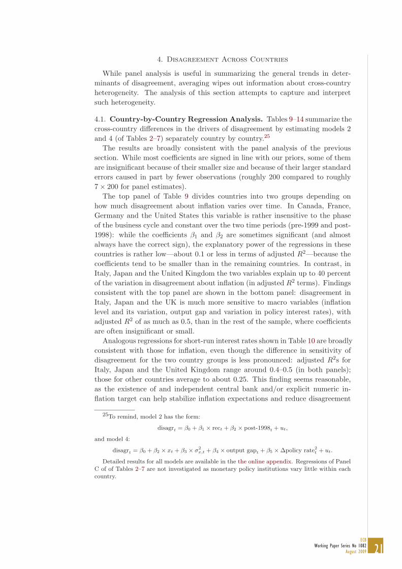
4. Disagreement Across Countries
While panel analysis is useful in summarizing the general trends in deter-minants of disagreement, averaging wipes out information about cross-countryheterogeneity. The analysis of this section attempts to capture and interpretsuch heterogeneity.
4.1. Country-by-Country Regression Analysis. Tables 9–14 summarize thecross-country differences in the drivers of disagreement by estimating models 2and 4 (of Tables 2–7) separately country by country.25
The results are broadly consistent with the panel analysis of the previoussection. While most coefficients are signed in line with our priors, some of themare insignificant because of their smaller size and because of their larger standarderrors caused in part by fewer observations (roughly 200 compared to roughly7× 200 for panel estimates).
The top panel of Table 9 divides countries into two groups depending onhow much disagreement about inflation varies over time. In Canada, France,Germany and the United States this variable is rather insensitive to the phaseof the business cycle and constant over the two time periods (pre-1999 and post-1998): while the coefficients β1 and β2 are sometimes significant (and almostalways have the correct sign), the explanatory power of the regressions in thesecountries is rather low—about 0.1 or less in terms of adjusted R2—because thecoefficients tend to be smaller than in the remaining countries. In contrast, inItaly, Japan and the United Kingdom the two variables explain up to 40 percentof the variation in disagreement about inflation (in adjusted R2 terms). Findingsconsistent with the top panel are shown in the bottom panel: disagreement inItaly, Japan and the UK is much more sensitive to macro variables (inflationlevel and its variation, output gap and variation in policy interest rates), withadjusted R2 of as much as 0.5, than in the rest of the sample, where coefficientsare often insignificant or small.
Analogous regressions for short-run interest rates shown in Table 10 are broadlyconsistent with those for inflation, even though the difference in sensitivity ofdisagreement for the two country groups is less pronounced: adjusted R2s forItaly, Japan and the United Kingdom range around 0.4–0.5 (in both panels);those for other countries average to about 0.25. This finding seems reasonable,as the existence of and independent central bank and/or explicit numeric in-flation target can help stabilize inflation expectations and reduce disagreement
25To remind, model 2 has the form:
disagrt = β0 + β1 × rect + β2 × post-1998t + ut,
and model 4:
disagrt = β0 + β2 × xt + β3 × σ2x,t + β4 × output gapt + β5 × Δpolicy rate2
t + ut.
Detailed results for all models are available in the the online appendix. Regressions of PanelC of of Tables 2–7 are not investigated as monetary policy institutions vary little within eachcountry.
22ECBWorking Paper Series No 1082August 2009
about inflation. In contrast, such targets are not announced for interest rates(or other variables).
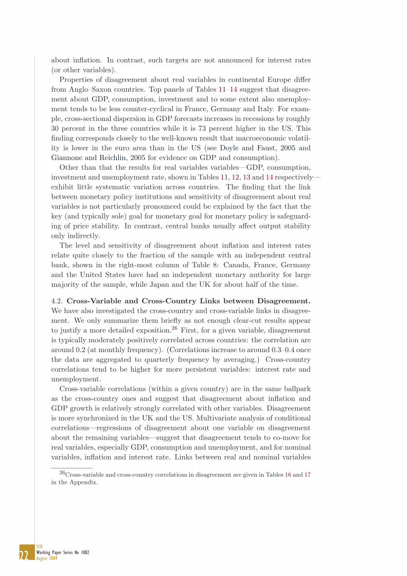
Properties of disagreement about real variables in continental Europe differfrom Anglo–Saxon countries. Top panels of Tables 11–14 suggest that disagree-ment about GDP, consumption, investment and to some extent also unemploy-ment tends to be less counter-cyclical in France, Germany and Italy. For exam-ple, cross-sectional dispersion in GDP forecasts increases in recessions by roughly30 percent in the three countries while it is 73 percent higher in the US. Thisfinding corresponds closely to the well-known result that macroeconomic volatil-ity is lower in the euro area than in the US (see Doyle and Faust, 2005 andGiannone and Reichlin, 2005 for evidence on GDP and consumption).
Other than that the results for real variables variables—GDP, consumption,investment and unemployment rate, shown in Tables 11, 12, 13 and 14 respectively—exhibit little systematic variation across countries. The finding that the linkbetween monetary policy institutions and sensitivity of disagreement about realvariables is not particularly pronounced could be explained by the fact that thekey (and typically sole) goal for monetary goal for monetary policy is safeguard-ing of price stability. In contrast, central banks usually affect output stabilityonly indirectly.
The level and sensitivity of disagreement about inflation and interest ratesrelate quite closely to the fraction of the sample with an independent centralbank, shown in the right-most column of Table 8: Canada, France, Germanyand the United States have had an independent monetary authority for largemajority of the sample, while Japan and the UK for about half of the time.
4.2. Cross-Variable and Cross-Country Links between Disagreement.We have also investigated the cross-country and cross-variable links in disagree-ment. We only summarize them briefly as not enough clear-cut results appearto justify a more detailed exposition.26 First, for a given variable, disagreementis typically moderately positively correlated across countries: the correlation arearound 0.2 (at monthly frequency). (Correlations increase to around 0.3–0.4 oncethe data are aggregated to quarterly frequency by averaging.) Cross-countrycorrelations tend to be higher for more persistent variables: interest rate andunemployment.
Cross-variable correlations (within a given country) are in the same ballparkas the cross-country ones and suggest that disagreement about inflation andGDP growth is relatively strongly correlated with other variables. Disagreementis more synchronized in the UK and the US. Multivariate analysis of conditionalcorrelations—regressions of disagreement about one variable on disagreementabout the remaining variables—suggest that disagreement tends to co-move forreal variables, especially GDP, consumption and unemployment, and for nominalvariables, inflation and interest rate. Links between real and nominal variables
26Cross-variable and cross-country correlations in disagreement are given in Tables 16 and 17in the Appendix.

23ECB
Working Paper Series No 1082August 2009
are less important (conditional on correlations between variables from the samegroup). We found little systematic pattern between countries in cross-countryconditional multivariate regressions (i.e., regressions of disagreement in one coun-try on disagreement in others for a given variable).
5. Turbulent Expectations 2008–2009
This section investigates in detail the dynamics of the cross-sectional distribu-tion of expectations during the ongoing financial turbulence. To describe thesedynamics we extend our data set until March 2009 and augment it with data forthe euro area.
Figure 20 illustrates the effects of the turmoil on disagreement about inflationand GDP growth.27 Although the recession in continental Europe and Japanhas according to CEPR’s business cycle dating committee and ECRI officiallystarted28 in the late 2007 or early 2008, substantial increase in disagreementoccurred only in the late 2008, following the fall of the investment bank LehmanBrothers in September, the considerable intensification of uncertainty on globalfinancial markets and the worsening of the macroeconomic outlook. By con-trast, disagreement about inflation and GDP in the US—the epicenter of theturbulence—gradually started to increase much earlier, right after the crisis brokein the summer 2007. Disagreement in the UK, whose financial sector is large andclosely linked with the US, evolved as an intermediate case between the US andcontinental Europe, starting to increase in the summer 2008. While before theturmoil the level of disagreement was roughly the same in all countries, the im-pact of the crisis on disagreement about GDP in Japan and disagreement aboutinflation in the UK and the US was significantly larger, reflecting sharper andlarger revisions of forecasts of these variables in the late 2008 and early 2009.29
Figures 21 and 22 display the cross-sectional distribution of GDP and infla-tion expectations (estimated using kernel density). The pre-crisis (June 2007)distribution of expectations is very peaked reflecting the widespread agreementamong forecasters. Before September 2008 expectations became more dispersedas the underlying variables moved and uncertainty was increasing. Comparisonof peaks of the distributions across regions suggests that expectations in the euroarea are more centered than in the UK and the US: For example, the probabil-ity weight on the mode of the euro area distribution of GDP (around 1) hastypically exceeded those in the UK and the US (around 0.7). (This observation
27Shaded areas again mark recessions as determined by ECRI and, for the euro area, byCEPR’s business cycle dating committee.
28We refer to the dates identified by CEPR’s business cycle dating committee for the euroarea, by NBER’s business cycle dating committee for the US, and by ECRI for other regions.
29For example, one-year ahead consensus expectations of GDP growth in Japan plummetedfrom 1.3 percent in August 2008 to −4.7 percent in March 2009. Consensus expectations ofinflation in the UK and the US, peaked in August 2008 at 3.8 and 3.6 percent respectivelybefore declining to 0.6 in the UK and −0.5 percent in the US in March 2009. (By comparison,inflation expectations in the euro area increased from roughly 2 percent before the crisis to 3percent in July 2008 and fell to 0.7 percent in March 2009.)

24ECBWorking Paper Series No 1082August 2009
remains broadly valid also for individual large euro area member countries shownin Figure 22.) The more spread-out distributions in the UK and US coincidewith more vigorous and volatile dynamics of the underlying variables and con-sensus expectations, in particular in the case of inflation (which has remainedmore stable in the euro area and its large members).30 Finally, the figures sug-gest that disagreement in most countries peaked in the early 2009 and decreasedsomewhat in March 2009.
6. Conclusion
Our estimates document a dichotomy between disagreement about real vari-ables (GDP, consumption, investment and unemployment), which is more stronglyaffected by real factors, and disagreement about nominal variables (inflation andinterest rate), which reacts to the institutional setting of monetary policy (in par-ticular central bank independence). Disagreement about real variables intensifiesstrongly during recessions. Disagreement about nominal variables is consider-ably lower under independent central banks. Cross-sectional dispersion for bothgroups increases with uncertainty about the underlying indicators. Country-by-country regressions for inflation and interest rates reveal that both the level ofdisagreement and its sensitivity to macroeconomic variables tend to be larger inItaly, Japan and the United Kingdom, where central banks became independentonly around the mid-1990s.
Our findings suggest that more credible monetary policy can substantially con-tribute to the anchoring of expectations about nominal variables; its effects ondisagreement about real variables are moderate. While our analysis uses data onexpectations of professional forecasters, qualitatively similar results may obtainalso for other economists (in industry, government and academia) and house-holds. This could be the case if our data are taken as a proxy for expectations ofthe rest of population, or if news spread epidemiologically from experts to otheragents (as proposed by Carroll, 2003).
To our knowledge, the results in this paper provide one of the first joint analy-ses of individual survey expectations across countries and variables. The strengthof some signals we use to investigate disagreement has been relatively weak: fol-lowing the Great Moderation, economic shocks in our sample (1989–2006) havebeen quite modest. Further insights about expectations and disagreement willbe gained once the data points covering the recent global turbulence accumulate.
References
Ager, Philipp, Marcus Kappler, and Steffen Osterloh (2009), “The Accuracy and Effi-ciency of the Consensus Forecasts: A Further Application and Extension of the PooledApproach,” International Journal of Forecasting, 25(1), 167–181.
30This is not the case in Germany, where the expected GDP growth was being revised quitesubstantially downward (compared to other euro area members and the US), reflecting in partthe country’s dependence on exports, and where disagreement intensified in the early 2009.

25ECB
Working Paper Series No 1082August 2009
Alesina, Alberto, and Roberta Gatti (1995), “Independent Central Banks: Low Inflationat No Cost?” American Economic Review, Papers and Proceedings, 85, 196–200.
Alesina, Alberto, and Lawrence H. Summers (1993), “Central Bank Independenceand Macroeconomic Performance: Some Comparative Evidence,” Journal of Money,Credit and Banking, 25, 151–162.
Ang, Andrew, Geert Bekaert, and Min Wei (2007), “Do Macro Variables, Asset Marketsor Surveys Forecast Inflation Better?” Journal of Monetary Economics, 54, 1163–1212.
Arnone, Marco, Bernard J. Laurens, Jean-Francois Segalotto, and Martin Sommer(2007), “Central Bank Autonomy: Lessons from Global Trends,” working paper 88,IMF.
Ball, Laurence (1992), “Why Does High Inflation Raise Inflation Uncertainty?” Journalof Monetary Economics, 29, 371–388.
Ball, Laurence, and Stephen Cecchetti (1990), “Inflation Uncertainty at Short and LongHorizons,” Brookings Papers on Economic Activity, 1, 251–254.
Batchelor, Roy (2007), “Bias in Macroeconomic Forecasts,” International Journal ofForecasting, 23, 189–203.
Beechey, Meredith J., Benjamin K. Johannsen, and Andrew T. Levin (2008), “AreLong-Run Inflation Expectations Anchored More Firmly in the Euro Area than inthe United States?” FEDS discussion paper 23, Federal Reserve Board.
Bernanke, Ben S. (2004), “The Logic of Monetary Policy,” remarks before the Nationaleconomists club, Federal Reserve Board.
Bernanke, Ben S., and Jean Boivin (2003), “Monetary Policy in a Data-Rich Environ-ment,” Journal of Monetary Economics, 50(3), 525–546.
Blanchflower, David G., and Roger Kelly (2008), “Macroeconomic Literacy, Numeracyand the Implications for Monetary Policy,” mimeo, Bank of England.
Bloom, Nicholas, Max Floetotto, and Nir Jaimovich (2009), “Really Uncertain BusinessCycles,” mimeo, Stanford University.
Branch, William A. (2004), “The Theory of Rationally Heterogeneous Expectations:Evidence from Survey Data on Inflation Expectations,” Economic Journal, 114(497),592–621.
Carroll, Christopher D. (1997), “Buffer-Stock Saving and the Life Cycle/PermanentIncome Hypothesis,” Quarterly Journal of Economics, 112(1), 1–55.
Carroll, Christopher D. (2003), “Macroeconomic Expectations of Households and Pro-fessional Forecasters,” Quarterly Journal of Economics, 118(1), 269–298.
Cogley, Timothy, and Thomas J. Sargent (2001), “Evolving Post-World War II U.S. In-flation Dynamics,” in Ben S. Bernanke and Kenneth Rogoff, editors, NBER Macroe-conomics Annual, volume 16, 331–388, NBER.
Creal, Drew, Siem Jan Koopman, and Eric Zivot (2008), “The Effect of the GreatModeration on the U.S. Business Cycle in a Time-Varying Multivariate Trend–CycleModel,” mimeo, Vrije Universiteit Amsterdam.
Crowe, Christopher, and Ellen E. Meade (2008), “Central Bank Independence andTransparency: Evolution and Effectiveness,” European Journal of Political Economy,24, 763–777.
Cukierman, Alex (1992), Central Bank Strategy, Credibility, and Independence, MITPress.
Devereux, Michael B., Gregor W. Smith, and James Yetman (2009), “Consumptionand Real Exchange Rates in Professional Forecasts,” working paper 1195, Queen’s

26ECBWorking Paper Series No 1082August 2009
University.Dopke, Jorg, and Ulrich Fritsche (2006), “When Do Forecasters Disagree? An Assess-
ment of German Growth and Inflation Forecast Dispersion,” International Journal ofForecasting, 22, 125–135.
Dovern, Jonas, and Ulrich Fritsche (2008), “Estimating Fundamental Cross-Section Dis-persion from Fixed Event Forecasts,” discussion paper 1, University Hamburg.
Doyle, Brian M., and Jon Faust (2005), “Breaks in the Variability and Co-movement ofG-7 Economic Growth,” Review of Economic and Statistics, 87(4), 721–740.
Ehrmann, Michael, Marcel Fratzscher, Refet S. Gurkaynak, and Eric T. Swanson (2007),“Convergence and Anchoring of Yield Curves in the Euro Area,” working paper 817,European Central Bank.
Engel, Charles, Nelson Mark, and Kenneth D. West (2008), “Exchange Rates ModelsAre Not As Bad As You Think,” in Daron Acemoglu, Kenneth Rogoff, and MichaelWoodford, editors, NBER Macroeconomics Annual 2007, volume 22, 381–441, Uni-versity of Chicago Press.
Engel, Charles, and John H. Rogers (2008), “Expected Consumption Growth fromCross-Country Surveys: Implications for Assessing International Capital Markets,”International Finance Discussion Paper 949, Federal Reserve System.
Erceg, Christopher J., and Andrew T. Levin (2003), “Imperfect Credibility and InflationPersistence,” Journal of Monetary Economics, 50(4), 915–944.
Faust, Jon, and Jonathan H. Wright (2007), “Comparing Greenbook Forecasts andReduced Form Forecasts using a Large Realtime Dataset,” working paper 13397,NBER.
Giannone, Domenico, and Lucrezia Reichlin (2005), “Euro Area and US Recessions,1970–2003,” in Lucrezia Reichlin, editor, The Euro Area Business Cycle: StylizedFacts and Measurement Issues, 83–93, CEPR.
Giordani, Paolo, and Robert Kohn (2008), “Efficient Bayesian Inference for MultipleChange-Point and Mixture Innovation Models,” Journal of Business and EconomicStatistics, 95(1), 66–77.
Grilli, Vittorio, Donato Masciandaro, and Guido Tabellini (1991), “Political and Mone-tary Institutions and Public Financial Policies in the Industrial Countries,” EconomicPolicy, 13, 341–392.
Gurkaynak, Refet S., Andrew T. Levin, and Eric T. Swanson (2006), “Does InflationTargeting Anchor Long-Run Inflation Expectations? Evidence from Long-Term BondYields in the US, UK and Sweden,” working paper 9, Federal Reserve Bank of SanFrancisco.
Harvey, Andrew C., and Thomas M. Trimbur (2003), “General Model-Based Filters forExtracting Cycles and Trends in Economic Time Series,” Review of Economics andStatistics, 85(2), 233–255.
Harvey, David I., Stephen J. Leybourne, and Paul Newbold (2001), “Analysis of a Panelof UK Macroeconomic Forecasts,” Econometrics Journal, 4(1), 37–55.
Iacoviello, Matteo (2005), “House Prices, Borrowing Constraints and Monetary Policyin the Business Cycle,” American Economic Review, 95(3), 739–764.
Isiklar, Gultekin, Kajal Lahiri, and Prakash Loungani (2006), “How Quickly Do Fore-casters Incorporate News? Evidence from Cross-country Surveys,” Journal of AppliedEconometrics, 21(6), 7033–725.
Kim, Don H., and Athanasios Orphanides (2005), “Term Structure Estimation withSurvey Data on Interest Rate Forecasts,” FEDS discussion paper 48, Federal Reserve

27ECB
Working Paper Series No 1082August 2009
Board.Krusell, Per, and Anthony A. Smith (1998), “Income and Wealth Heterogeneity in the
Macroeconomy,” Journal of Political Economy, 106(5), 867–896.Lahiri, Kajal, and Xuguang Sheng (2009), “Measuring Forecast Uncertainty by Dis-
agreement: The Missing Link,” Journal of Applied Econometrics, forthcoming.Levin, Andrew T., Fabio M. Natalucci, and Jeremy M. Piger (2004), “Explicit Inflation
Objectives and Macroeconomic Outcomes,” working paper 383, European CentralBank.
Mankiw, N. Gregory, Ricardo Reis, and Justin Wolfers (2003), “Disagreement on Infla-tion Expectations,” NBER Macroeconomics Annual, 209–248.
Morris, Stephen, and Hyun Song Shin (2005a), “Central Bank Transparency and theSignal Value of Prices,” Brookings Papers on Economic Activity, 2, 1–66.
Morris, Stephen, and Hyun Song Shin (2005b), “The Social Value of Public Informa-tion,” American Economic Review, 92, 1521–1534.
Patton, Andrew J., and Allan Timmermann (2008a), “The Resolution of MacroeconomicUncertainty: Evidence from Survey Forecasts,” mimeo, University of Oxford.
Patton, Andrew J., and Allan Timmermann (2008b), “Why Do Forecasters Disagree?Lessons from the Term Structure of Cross-Sectional Dispersion,” mimeo, Universityof Oxford.
Piazzesi, Monika, and Martin Schneider (2008), “Bond Positions, Expectations, and theYield Curve,” working paper 2, Federal Reserve Bank of Atlanta.
Rogoff, Kenneth (1985), “The Optimal Degree of Commitment to an Intermediate Mon-etary Target,” Quarterly Journal of Economics, 100, 1169–1190.
Scheinkman, Jose, and Wei Xiong (2003), “Heterogeneous Beliefs, Speculation and Trad-ing in Financial Markets,” in Paris–Princeton Lectures on Mathematical Finance,volume 1847, Springer.
Souleles, Nicholas S. (2004), “Expectations, Heterogeneous Forecast Errors, and Con-sumption: Micro Evidence from the Michigan Consumer Sentiment Surveys,” Journalof Money, Credit and Banking, 36(1), 39–72.
Stock, James H., and Mark W. Watson (2002), “Has the Business Cycle Changed andWhy?” in Mark Gertler and Ken Rogoff, editors, NBER Macroeconomics Annual,MIT Press.
Stock, James H., and Mark W. Watson (2005), “Understanding Changes in InternationalBusiness Cycle Dynamics,” Journal of the European Economic Association, 3, 968–1006.
Stock, James H., and Mark W. Watson (2007), “Why Has U.S. Inflation Become Harderto Forecast?” Journal of Money, Credit, and Banking, 39, 3–33.
Woodford, Michael (2005), “Central Bank Communication and Policy Effectiveness,”working paper 11898, NBER.
Wright, Jonathan H. (2008), “Term Premiums and Inflation Uncertainty: EmpiricalEvidence from an International Dataset,” FEDS Discussion Paper 25, Federal ReserveBoard.
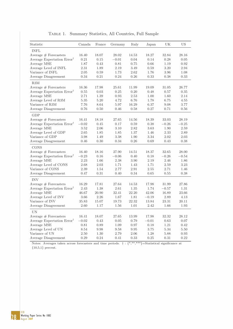
28ECBWorking Paper Series No 1082August 2009
Table 1. Summary Statistics, All Countries, Full Sample
Statistic Canada France Germany Italy Japan UK US
INFLAverage # Forecasters 16.40 18.07 28.02 14.53 18.27 32.84 28.16
Average Expectation Error† 0.21 0.15 −0.01 0.04 0.14 0.28 0.05Average MSE 1.87 0.43 0.81 0.75 0.66 1.19 0.92Average Level of INFL 2.31 1.89 2.19 3.49 0.59 3.20 2.94Variance of INFL 2.05 0.59 1.73 2.62 1.76 3.96 1.08Average Disagreement 0.34 0.21 0.24 0.26 0.33 0.38 0.33
R3MAverage # Forecasters 16.36 17.98 25.61 11.99 19.09 31.05 26.77
Average Expectation Error† 0.55 0.03 0.25 0.20 0.48 0.57 0.35Average MSE 2.71 1.39 0.93 2.53 1.00 1.60 2.14Average Level of R3M 5.35 5.20 4.72 6.76 1.78 6.75 4.55Variance of R3M 7.76 8.64 5.97 16.29 6.37 9.08 3.77Average Disagreement 0.76 0.50 0.46 0.58 0.27 0.71 0.56
GDPAverage # Forecasters 16.41 18.18 27.65 14.56 18.39 33.03 28.19
Average Expectation Error† −0.02 0.45 0.17 0.59 0.38 −0.26 −0.25Average MSE 3.52 2.06 3.10 2.82 3.63 1.90 2.59Average Level of GDP 2.65 1.85 1.85 1.37 1.46 2.33 2.89Variance of GDP 3.98 1.49 3.38 1.90 3.34 2.02 2.03Average Disagreement 0.46 0.30 0.34 0.26 0.69 0.43 0.38
CONSAverage # Forecasters 16.40 18.16 27.90 14.51 18.37 32.65 28.00
Average Expectation Error† −0.23 0.16 −0.06 0.40 0.18 −0.26 −0.54Average MSE 2.23 1.66 2.38 3.90 2.19 2.46 1.86Average Level of CONS 2.68 2.03 1.71 1.43 1.71 2.59 3.23Variance of CONS 2.39 1.54 2.77 2.91 2.55 2.71 1.46Average Disagreement 0.47 0.31 0.40 0.34 0.65 0.55 0.38
INVAverage # Forecasters 16.29 17.81 27.64 14.53 17.98 31.99 27.86
Average Expectation Error† 2.43 1.38 2.61 1.35 1.74 −0.57 1.31Average MSE 46.67 20.90 32.41 22.20 42.06 16.89 23.66Average Level of INV 3.66 2.26 1.67 1.81 −0.19 2.89 4.13Variance of INV 35.83 15.07 19.73 22.32 13.84 23.31 20.11Average Disagreement 2.60 1.17 1.56 1.01 2.42 1.66 1.93
UNAverage # Forecasters 16.41 18.07 27.65 13.99 17.98 32.32 28.12
Average Expectation Error† −0.02 0.43 0.05 0.79 −0.01 0.63 0.07Average MSE 0.81 0.89 1.09 0.97 0.18 1.21 0.42Average Level of UN 8.54 9.98 9.58 9.95 3.75 5.34 5.50Variance of UN 2.50 1.30 2.79 2.06 1.28 5.88 0.93Average Disagreement 0.29 0.24 0.41 0.33 0.25 0.31 0.22
Notes: Averages taken across forecasters and time periods. † : {*,**,***}=Statistical significance at
{10,5,1} percent.
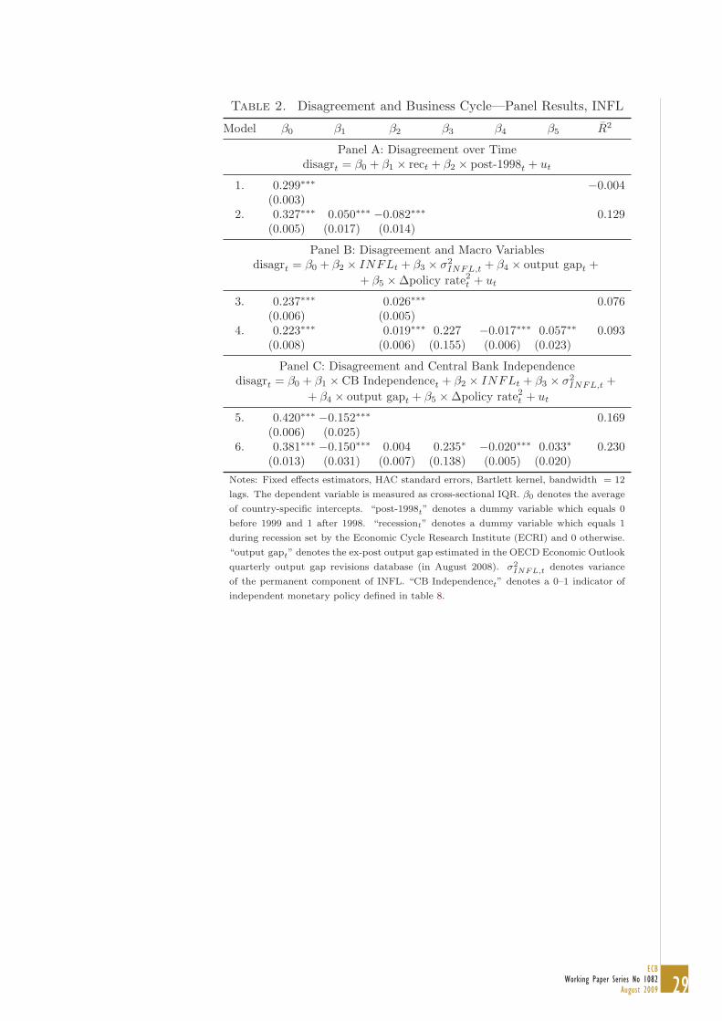
29ECB
Working Paper Series No 1082August 2009
Table 2. Disagreement and Business Cycle—Panel Results, INFL
Model β0 β1 β2 β3 β4 β5 R2
Panel A: Disagreement over Timedisagrt = β0 + β1 × rect + β2 × post-1998t + ut
1. 0.299∗∗∗ −0.004(0.003)
2. 0.327∗∗∗ 0.050∗∗∗ −0.082∗∗∗ 0.129(0.005) (0.017) (0.014)
Panel B: Disagreement and Macro Variablesdisagrt = β0 + β2 × INFLt + β3 × σ2
INFL,t + β4 × output gapt ++ β5 ×Δpolicy rate2
t + ut
3. 0.237∗∗∗ 0.026∗∗∗ 0.076(0.006) (0.005)
4. 0.223∗∗∗ 0.019∗∗∗ 0.227 −0.017∗∗∗ 0.057∗∗ 0.093(0.008) (0.006) (0.155) (0.006) (0.023)
Panel C: Disagreement and Central Bank Independencedisagrt = β0 + β1 × CB Independencet + β2 × INFLt + β3 × σ2
INFL,t ++ β4 × output gapt + β5 ×Δpolicy rate2
t + ut
5. 0.420∗∗∗ −0.152∗∗∗ 0.169(0.006) (0.025)
6. 0.381∗∗∗ −0.150∗∗∗ 0.004 0.235∗ −0.020∗∗∗ 0.033∗ 0.230(0.013) (0.031) (0.007) (0.138) (0.005) (0.020)
Notes: Fixed effects estimators, HAC standard errors, Bartlett kernel, bandwidth = 12
lags. The dependent variable is measured as cross-sectional IQR. β0 denotes the average
of country-specific intercepts. “post-1998t” denotes a dummy variable which equals 0
before 1999 and 1 after 1998. “recessiont” denotes a dummy variable which equals 1
during recession set by the Economic Cycle Research Institute (ECRI) and 0 otherwise.
“output gapt” denotes the ex-post output gap estimated in the OECD Economic Outlook
quarterly output gap revisions database (in August 2008). σ2INFL,t denotes variance
of the permanent component of INFL. “CB Independencet” denotes a 0–1 indicator of
independent monetary policy defined in table 8.
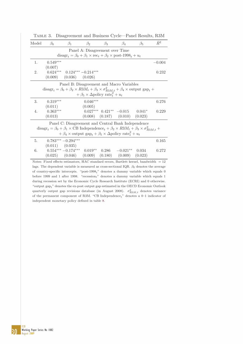
30ECBWorking Paper Series No 1082August 2009
Table 3. Disagreement and Business Cycle—Panel Results, R3M
Model β0 β1 β2 β3 β4 β5 R2
Panel A: Disagreement over Timedisagrt = β0 + β1 × rect + β2 × post-1998t + ut
1. 0.549∗∗∗ −0.004(0.007)
2. 0.624∗∗∗ 0.124∗∗∗ −0.214∗∗∗ 0.232(0.009) (0.036) (0.026)
Panel B: Disagreement and Macro Variablesdisagrt = β0 + β2 ×R3Mt + β3 × σ2
R3M,t + β4 × output gapt ++ β5 ×Δpolicy rate2
t + ut
3. 0.319∗∗∗ 0.046∗∗∗ 0.276(0.011) (0.005)
4. 0.363∗∗∗ 0.027∗∗∗ 0.421∗∗ −0.015 0.041∗ 0.229(0.013) (0.008) (0.187) (0.010) (0.023)
Panel C: Disagreement and Central Bank Independencedisagrt = β0 + β1 × CB Independencet + β2 ×R3Mt + β3 × σ2
R3M,t ++ β4 × output gapt + β5 ×Δpolicy rate2
t + ut
5. 0.783∗∗∗ −0.294∗∗∗ 0.165(0.011) (0.035)
6. 0.554∗∗∗ −0.174∗∗∗ 0.019∗∗ 0.286 −0.021∗∗ 0.034 0.272(0.025) (0.046) (0.009) (0.180) (0.009) (0.023)
Notes: Fixed effects estimators, HAC standard errors, Bartlett kernel, bandwidth = 12
lags. The dependent variable is measured as cross-sectional IQR. β0 denotes the average
of country-specific intercepts. “post-1998t” denotes a dummy variable which equals 0
before 1999 and 1 after 1998. “recessiont” denotes a dummy variable which equals 1
during recession set by the Economic Cycle Research Institute (ECRI) and 0 otherwise.
“output gapt” denotes the ex-post output gap estimated in the OECD Economic Outlook
quarterly output gap revisions database (in August 2008). σ2R3M,t denotes variance
of the permanent component of R3M. “CB Independencet” denotes a 0–1 indicator of
independent monetary policy defined in table 8.

31ECB
Working Paper Series No 1082August 2009
Table 4. Disagreement and Business Cycle—Panel Results, GDP
Model β0 β1 β2 β3 β4 β5 R2
Panel A: Disagreement over Timedisagrt = β0 + β1 × rect + β2 × post-1998t + ut
1. 0.410∗∗∗ −0.004(0.004)
2. 0.394∗∗∗ 0.160∗∗∗ −0.032∗ 0.134(0.006) (0.027) (0.018)
Panel B: Disagreement and Macro Variablesdisagrt = β0 + β2 ×GDPt + β3 × σ2
GDP,t + β4 × output gapt ++ β5 ×Δpolicy rate2
t + ut
3. 0.482∗∗∗ −0.035∗∗∗ 0.107(0.007) (0.006)
4. 0.379∗∗∗ −0.025∗∗∗ 0.686∗∗∗ −0.001 0.048 0.136(0.013) (0.007) (0.180) (0.007) (0.035)
Panel C: Disagreement and Central Bank Independencedisagrt = β0 + β1 × CB Independencet + β2 ×GDPt + β3 × σ2
GDP,t ++ β4 × output gapt + β5 ×Δpolicy rate2
t + ut
5. 0.458∗∗∗ −0.061∗ 0.010(0.007) (0.034)
6. 0.424∗∗∗ −0.060∗ −0.023∗∗∗ 0.677∗∗∗ −0.004 0.038 0.149(0.017) (0.031) (0.006) (0.178) (0.007) (0.033)
Notes: Fixed effects estimators, HAC standard errors, Bartlett kernel, bandwidth = 12
lags. The dependent variable is measured as cross-sectional IQR. β0 denotes the average
of country-specific intercepts. “post-1998t” denotes a dummy variable which equals 0
before 1999 and 1 after 1998. “recessiont” denotes a dummy variable which equals 1
during recession set by the Economic Cycle Research Institute (ECRI) and 0 otherwise.
“output gapt” denotes the ex-post output gap estimated in the OECD Economic Outlook
quarterly output gap revisions database (in August 2008). σ2GDP,t denotes variance
of the permanent component of GDP. “CB Independencet” denotes a 0–1 indicator of
independent monetary policy defined in table 8.

32ECBWorking Paper Series No 1082August 2009
Table 5. Disagreement and Business Cycle—Panel Results, CONS
Model β0 β1 β2 β3 β4 β5 R2
Panel A: Disagreement over Timedisagrt = β0 + β1 × rect + β2 × post-1998t + ut
1. 0.445∗∗∗ −0.004(0.004)
2. 0.419∗∗∗ 0.161∗∗∗ −0.012 0.128(0.006) (0.024) (0.015)
Panel B: Disagreement and Macro Variablesdisagrt = β0 + β2 × CONSt + β3 × σ2
CONS,t + β4 × output gapt ++ β5 ×Δpolicy rate2
t + ut
3. 0.512∗∗∗ −0.031∗∗∗ 0.073(0.007) (0.007)
4. 0.452∗∗∗ −0.023∗∗∗ 0.262∗∗∗ −0.002 0.044∗ 0.088(0.011) (0.008) (0.077) (0.007) (0.024)
Panel C: Disagreement and Central Bank Independencedisagrt = β0 + β1 × CB Independencet + β2 × CONSt + β3 × σ2
CONS,t ++ β4 × output gapt + β5 ×Δpolicy rate2
t + ut
5. 0.469∗∗∗ −0.031 −0.001(0.007) (0.030)
6. 0.458∗∗∗ −0.007 −0.023∗∗∗ 0.256∗∗∗ −0.002 0.043∗ 0.088(0.017) (0.031) (0.008) (0.082) (0.007) (0.024)
Notes: Fixed effects estimators, HAC standard errors, Bartlett kernel, bandwidth = 12
lags. The dependent variable is measured as cross-sectional IQR. β0 denotes the average
of country-specific intercepts. “post-1998t” denotes a dummy variable which equals 0
before 1999 and 1 after 1998. “recessiont” denotes a dummy variable which equals 1
during recession set by the Economic Cycle Research Institute (ECRI) and 0 otherwise.
“output gapt” denotes the ex-post output gap estimated in the OECD Economic Outlook
quarterly output gap revisions database (in August 2008). σ2CONS,t denotes variance of
the permanent component of CONS. “CB Independencet” denotes a 0–1 indicator of
independent monetary policy defined in table 8.
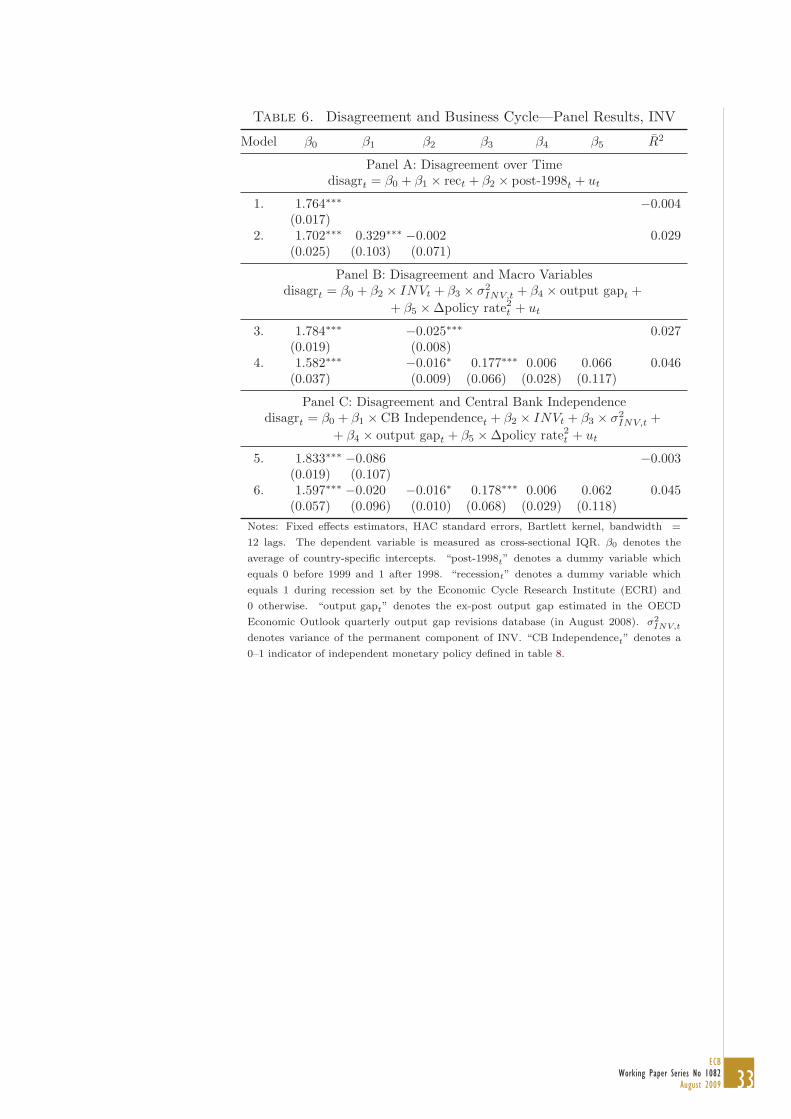
33ECB
Working Paper Series No 1082August 2009
Table 6. Disagreement and Business Cycle—Panel Results, INV
Model β0 β1 β2 β3 β4 β5 R2
Panel A: Disagreement over Timedisagrt = β0 + β1 × rect + β2 × post-1998t + ut
1. 1.764∗∗∗ −0.004(0.017)
2. 1.702∗∗∗ 0.329∗∗∗ −0.002 0.029(0.025) (0.103) (0.071)
Panel B: Disagreement and Macro Variablesdisagrt = β0 + β2 × INVt + β3 × σ2
INV,t + β4 × output gapt ++ β5 ×Δpolicy rate2
t + ut
3. 1.784∗∗∗ −0.025∗∗∗ 0.027(0.019) (0.008)
4. 1.582∗∗∗ −0.016∗ 0.177∗∗∗ 0.006 0.066 0.046(0.037) (0.009) (0.066) (0.028) (0.117)
Panel C: Disagreement and Central Bank Independencedisagrt = β0 + β1 × CB Independencet + β2 × INVt + β3 × σ2
INV,t ++ β4 × output gapt + β5 ×Δpolicy rate2
t + ut
5. 1.833∗∗∗ −0.086 −0.003(0.019) (0.107)
6. 1.597∗∗∗ −0.020 −0.016∗ 0.178∗∗∗ 0.006 0.062 0.045(0.057) (0.096) (0.010) (0.068) (0.029) (0.118)
Notes: Fixed effects estimators, HAC standard errors, Bartlett kernel, bandwidth =
12 lags. The dependent variable is measured as cross-sectional IQR. β0 denotes the
average of country-specific intercepts. “post-1998t” denotes a dummy variable which
equals 0 before 1999 and 1 after 1998. “recessiont” denotes a dummy variable which
equals 1 during recession set by the Economic Cycle Research Institute (ECRI) and
0 otherwise. “output gapt” denotes the ex-post output gap estimated in the OECD
Economic Outlook quarterly output gap revisions database (in August 2008). σ2INV,t
denotes variance of the permanent component of INV. “CB Independencet” denotes a
0–1 indicator of independent monetary policy defined in table 8.

34ECBWorking Paper Series No 1082August 2009
Table 7. Disagreement and Business Cycle—Panel Results, UN
Model β0 β1 β2 β3 β4 β5 R2
Panel A: Disagreement over Timedisagrt = β0 + β1 × rect + β2 × post-1998t + ut
1. 0.293∗∗∗ −0.004(0.005)
2. 0.297∗∗∗ 0.156∗∗∗ −0.074∗∗∗ 0.169(0.006) (0.041) (0.018)
Panel B: Disagreement and Macro Variablesdisagrt = β0 + β2 × UNt + β3 × σ2
UN,t + β4 × output gapt ++ β5 ×Δpolicy rate2
t + ut
3. 0.302∗∗∗ −0.001 −0.005(0.023) (0.013)
4. 0.432∗∗∗ −0.034∗ 7.857∗∗∗ −0.009 −0.017 0.162(0.027) (0.020) (1.927) (0.008) (0.014)
Panel C: Disagreement and Central Bank Independencedisagrt = β0 + β1 × CB Independencet + β2 × UNt + β3 × σ2
UN,t ++ β4 × output gapt + β5 ×Δpolicy rate2
t + ut
5. 0.344∗∗∗ −0.064∗∗ 0.011(0.023) (0.029)
6. 0.506∗∗∗ −0.050 −0.037∗ 7.284∗∗∗ −0.015∗ −0.023∗ 0.168(0.036) (0.032) (0.020) (1.874) (0.009) (0.014)
Notes: Fixed effects estimators, HAC standard errors, Bartlett kernel, bandwidth =
12 lags. The dependent variable is measured as cross-sectional IQR. β0 denotes the
average of country-specific intercepts. “post-1998t” denotes a dummy variable which
equals 0 before 1999 and 1 after 1998. “recessiont” denotes a dummy variable which
equals 1 during recession set by the Economic Cycle Research Institute (ECRI) and
0 otherwise. “output gapt” denotes the ex-post output gap estimated in the OECD
Economic Outlook quarterly output gap revisions database (in August 2008). σ2UN,t
denotes variance of the permanent component of UN. “CB Independencet” denotes a
0–1 indicator of independent monetary policy defined in table 8.
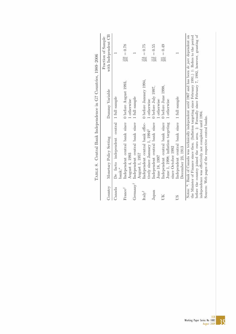
35ECB
Working Paper Series No 1082August 2009
Table
8.
Cen
tral
Ban
kIn
depe
nden
cein
G7
Cou
ntri
es,19
89–2
006
Frac
tion
ofSa
mpl
eC
ount
ryM
onet
ary
Pol
icy
Sett
ing
Dum
my
Var
iabl
ew
ith
Inde
pend
ent
CB
Can
ada
De
fact
oin
depe
nden
tce
ntra
lba
nk;∗
1fu
llsa
mpl
e1
Fran
ce†
Inde
pend
ent
cent
ral
bank
sinc
eA
ugus
t4,
1993
0be
fore
Aug
ust
1993
,1
othe
rwis
e
159
205
=0.
78
Ger
man
y†In
depe
nden
tce
ntra
lba
nksi
nce
Aug
ust
1,19
571
full
sam
ple
1
Ital
y†In
depe
nden
tce
ntra
lba
nkeff
ec-
tive
lysi
nce
Janu
ary
1,19
94‡
0be
fore
Janu
ary
1994
,1
othe
rwis
e
154
205
=0.
75
Japa
nIn
depe
nden
tce
ntra
lba
nksi
nce
June
18,19
970
befo
reJu
ly19
97,
1ot
herw
ise
112
205
=0.
55
UK
Inde
pend
ent
cent
ral
bank
sinc
eJu
ne1,
1998
;in
flati
onta
rget
ing
sinc
eO
ctob
er19
92
0be
fore
June
1998
,1
othe
rwis
e
101
205
=0.
49
US
Inde
pend
ent
cent
ral
bank
sinc
eD
ecem
ber
23,19
131
full
sam
ple
1
Note
s:*:
Bank
ofC
anada
was
tech
nic
ally
indep
enden
tuntil
1967
and
has
bee
nde
jure
dep
enden
ton
the
Min
iste
rofFin
ance
since
then
.(I
nflati
on
targ
etin
gsi
nce
Feb
ruary
1991.)
†:R
efer
sto
the
per
iod
bef
ore
the
countr
yjo
ined
the
euro
are
a.
‡:Form
ally
since
Feb
ruary
7,
1992,
how
ever
,gra
nti
ng
of
indep
enden
cew
as
effec
tivel
ynot
com
ple
ted
unti
l1994.
Sourc
es:
Web
pages
ofth
ere
spec
tive
centr
albanks.
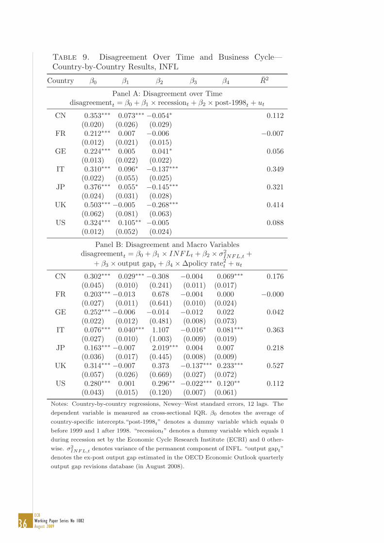
36ECBWorking Paper Series No 1082August 2009
Table 9. Disagreement Over Time and Business Cycle—Country-by-Country Results, INFL
Country β0 β1 β2 β3 β4 R2
Panel A: Disagreement over Timedisagreementt = β0 + β1 × recessiont + β2 × post-1998t + ut
CN 0.353∗∗∗ 0.073∗∗∗ −0.054∗ 0.112(0.020) (0.026) (0.029)
FR 0.212∗∗∗ 0.007 −0.006 −0.007(0.012) (0.021) (0.015)
GE 0.224∗∗∗ 0.005 0.041∗ 0.056(0.013) (0.022) (0.022)
IT 0.310∗∗∗ 0.096∗ −0.137∗∗∗ 0.349(0.022) (0.055) (0.025)
JP 0.376∗∗∗ 0.055∗ −0.145∗∗∗ 0.321(0.024) (0.031) (0.028)
UK 0.503∗∗∗ −0.005 −0.268∗∗∗ 0.414(0.062) (0.081) (0.063)
US 0.324∗∗∗ 0.105∗∗ −0.005 0.088(0.012) (0.052) (0.024)
Panel B: Disagreement and Macro Variablesdisagreementt = β0 + β1 × INFLt + β2 × σ2
INFL,t ++ β3 × output gapt + β4 ×Δpolicy rate2
t + ut
CN 0.302∗∗∗ 0.029∗∗∗ −0.308 −0.004 0.069∗∗∗ 0.176(0.045) (0.010) (0.241) (0.011) (0.017)
FR 0.203∗∗∗ −0.013 0.678 −0.004 0.000 −0.000(0.027) (0.011) (0.641) (0.010) (0.024)
GE 0.252∗∗∗ −0.006 −0.014 −0.012 0.022 0.042(0.022) (0.012) (0.481) (0.008) (0.073)
IT 0.076∗∗∗ 0.040∗∗∗ 1.107 −0.016∗ 0.081∗∗∗ 0.363(0.027) (0.010) (1.003) (0.009) (0.019)
JP 0.163∗∗∗ −0.007 2.019∗∗∗ 0.004 0.007 0.218(0.036) (0.017) (0.445) (0.008) (0.009)
UK 0.314∗∗∗ −0.007 0.373 −0.137∗∗∗ 0.233∗∗∗ 0.527(0.057) (0.026) (0.669) (0.027) (0.072)
US 0.280∗∗∗ 0.001 0.296∗∗ −0.022∗∗∗ 0.120∗∗ 0.112(0.043) (0.015) (0.120) (0.007) (0.061)
Notes: Country-by-country regressions, Newey–West standard errors, 12 lags. The
dependent variable is measured as cross-sectional IQR. β0 denotes the average of
country-specific intercepts.“post-1998t” denotes a dummy variable which equals 0
before 1999 and 1 after 1998. “recessiont” denotes a dummy variable which equals 1
during recession set by the Economic Cycle Research Institute (ECRI) and 0 other-
wise. σ2INFL,t denotes variance of the permanent component of INFL. “output gapt”
denotes the ex-post output gap estimated in the OECD Economic Outlook quarterly
output gap revisions database (in August 2008).

37ECB
Working Paper Series No 1082August 2009
Table 10. Disagreement Over Time and Business Cycle—Country-by-Country Results, R3M
Country β0 β1 β2 β3 β4 R2
Panel A: Disagreement over Timedisagreementt = β0 + β1 × recessiont + β2 × post-1998t + ut
CN 0.885∗∗∗ 0.190 −0.328∗∗∗ 0.295(0.084) (0.187) (0.093)
FR 0.514∗∗∗ 0.231∗∗ −0.101∗∗ 0.221(0.033) (0.111) (0.042)
GE 0.477∗∗∗ 0.110∗∗ −0.126∗∗ 0.191(0.054) (0.049) (0.049)
IT 0.720∗∗∗ 0.149∗ −0.341∗∗∗ 0.405(0.050) (0.080) (0.052)
JP 0.417∗∗∗ −0.052 −0.267∗∗∗ 0.513(0.026) (0.041) (0.050)
UK 0.827∗∗∗ 0.208∗∗ −0.299∗∗∗ 0.399(0.074) (0.086) (0.078)
US 0.549∗∗∗ 0.124∗∗∗ 0.008 0.031(0.035) (0.044) (0.056)
Panel B: Disagreement and Macro Variablesdisagreementt = β0 + β1 ×R3Mt + β2 × σ2
R3M,t ++ β3 × output gapt + β4 ×Δpolicy rate2
t + ut
CN 0.543∗∗∗ 0.026 −0.263 −0.053∗∗ 0.075∗∗ 0.213(0.079) (0.021) (0.574) (0.026) (0.036)
FR 0.444∗∗∗ −0.018∗ 1.695∗∗∗ 0.007 0.030 0.460(0.037) (0.010) (0.393) (0.016) (0.090)
GE 0.232∗∗∗ 0.041∗∗∗ 0.886 −0.032∗∗∗ −0.046 0.248(0.053) (0.015) (1.297) (0.011) (0.198)
IT 0.251∗∗∗ 0.045∗∗ 0.053 −0.045∗∗∗ 0.008 0.435(0.057) (0.018) (0.281) (0.012) (0.067)
JP 0.243∗∗∗ −0.021 1.798 0.071∗∗∗ 0.020 0.580(0.025) (0.015) (2.289) (0.011) (0.012)
UK 0.634∗∗∗ −0.020 3.187∗∗∗ −0.109∗∗∗ −0.102 0.463(0.105) (0.022) (1.100) (0.037) (0.086)
US 0.625∗∗∗ −0.024 0.441 −0.007 0.112 0.058(0.072) (0.015) (0.972) (0.019) (0.095)
Notes: Country-by-country regressions, Newey–West standard errors, 12 lags. The
dependent variable is measured as cross-sectional IQR. β0 denotes the average of
country-specific intercepts.“post-1998t” denotes a dummy variable which equals 0
before 1999 and 1 after 1998. “recessiont” denotes a dummy variable which equals 1
during recession set by the Economic Cycle Research Institute (ECRI) and 0 other-
wise. σ2R3M,t denotes variance of the permanent component of R3M. “output gapt”
denotes the ex-post output gap estimated in the OECD Economic Outlook quarterly
output gap revisions database (in August 2008).
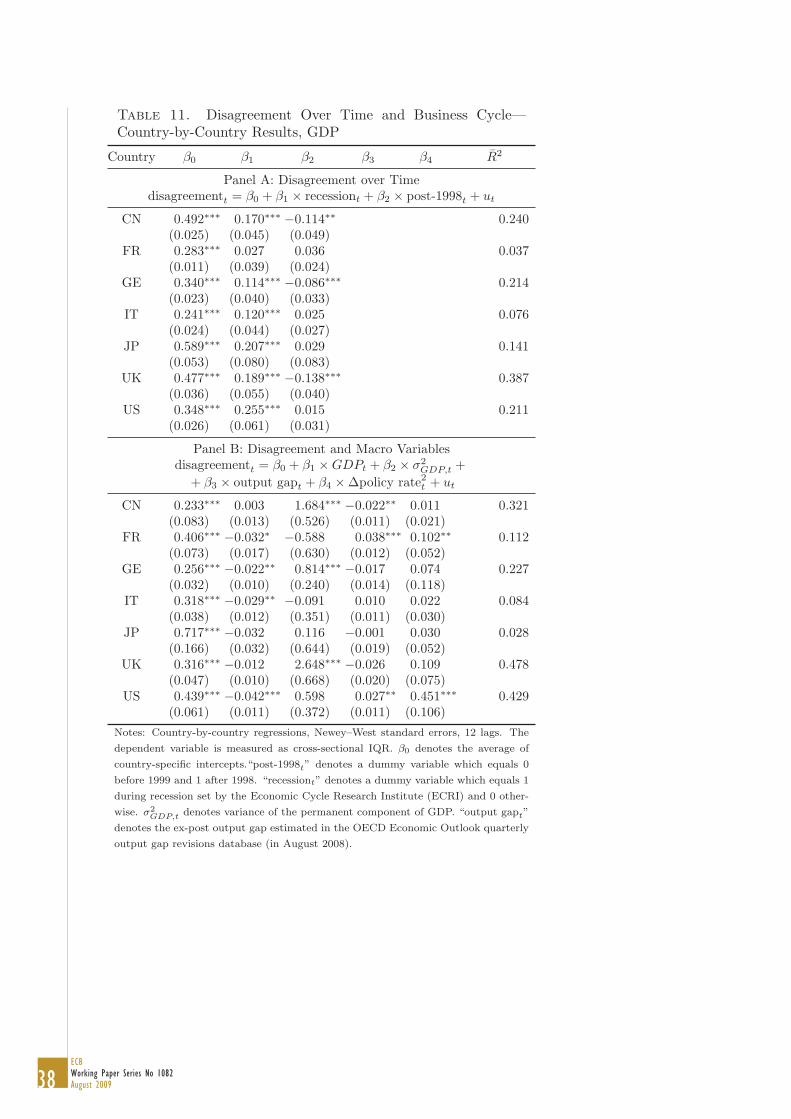
38ECBWorking Paper Series No 1082August 2009
Table 11. Disagreement Over Time and Business Cycle—Country-by-Country Results, GDP
Country β0 β1 β2 β3 β4 R2
Panel A: Disagreement over Timedisagreementt = β0 + β1 × recessiont + β2 × post-1998t + ut
CN 0.492∗∗∗ 0.170∗∗∗ −0.114∗∗ 0.240(0.025) (0.045) (0.049)
FR 0.283∗∗∗ 0.027 0.036 0.037(0.011) (0.039) (0.024)
GE 0.340∗∗∗ 0.114∗∗∗ −0.086∗∗∗ 0.214(0.023) (0.040) (0.033)
IT 0.241∗∗∗ 0.120∗∗∗ 0.025 0.076(0.024) (0.044) (0.027)
JP 0.589∗∗∗ 0.207∗∗∗ 0.029 0.141(0.053) (0.080) (0.083)
UK 0.477∗∗∗ 0.189∗∗∗ −0.138∗∗∗ 0.387(0.036) (0.055) (0.040)
US 0.348∗∗∗ 0.255∗∗∗ 0.015 0.211(0.026) (0.061) (0.031)
Panel B: Disagreement and Macro Variablesdisagreementt = β0 + β1 ×GDPt + β2 × σ2
GDP,t ++ β3 × output gapt + β4 ×Δpolicy rate2
t + ut
CN 0.233∗∗∗ 0.003 1.684∗∗∗ −0.022∗∗ 0.011 0.321(0.083) (0.013) (0.526) (0.011) (0.021)
FR 0.406∗∗∗ −0.032∗ −0.588 0.038∗∗∗ 0.102∗∗ 0.112(0.073) (0.017) (0.630) (0.012) (0.052)
GE 0.256∗∗∗ −0.022∗∗ 0.814∗∗∗ −0.017 0.074 0.227(0.032) (0.010) (0.240) (0.014) (0.118)
IT 0.318∗∗∗ −0.029∗∗ −0.091 0.010 0.022 0.084(0.038) (0.012) (0.351) (0.011) (0.030)
JP 0.717∗∗∗ −0.032 0.116 −0.001 0.030 0.028(0.166) (0.032) (0.644) (0.019) (0.052)
UK 0.316∗∗∗ −0.012 2.648∗∗∗ −0.026 0.109 0.478(0.047) (0.010) (0.668) (0.020) (0.075)
US 0.439∗∗∗ −0.042∗∗∗ 0.598 0.027∗∗ 0.451∗∗∗ 0.429(0.061) (0.011) (0.372) (0.011) (0.106)
Notes: Country-by-country regressions, Newey–West standard errors, 12 lags. The
dependent variable is measured as cross-sectional IQR. β0 denotes the average of
country-specific intercepts.“post-1998t” denotes a dummy variable which equals 0
before 1999 and 1 after 1998. “recessiont” denotes a dummy variable which equals 1
during recession set by the Economic Cycle Research Institute (ECRI) and 0 other-
wise. σ2GDP,t denotes variance of the permanent component of GDP. “output gapt”
denotes the ex-post output gap estimated in the OECD Economic Outlook quarterly
output gap revisions database (in August 2008).
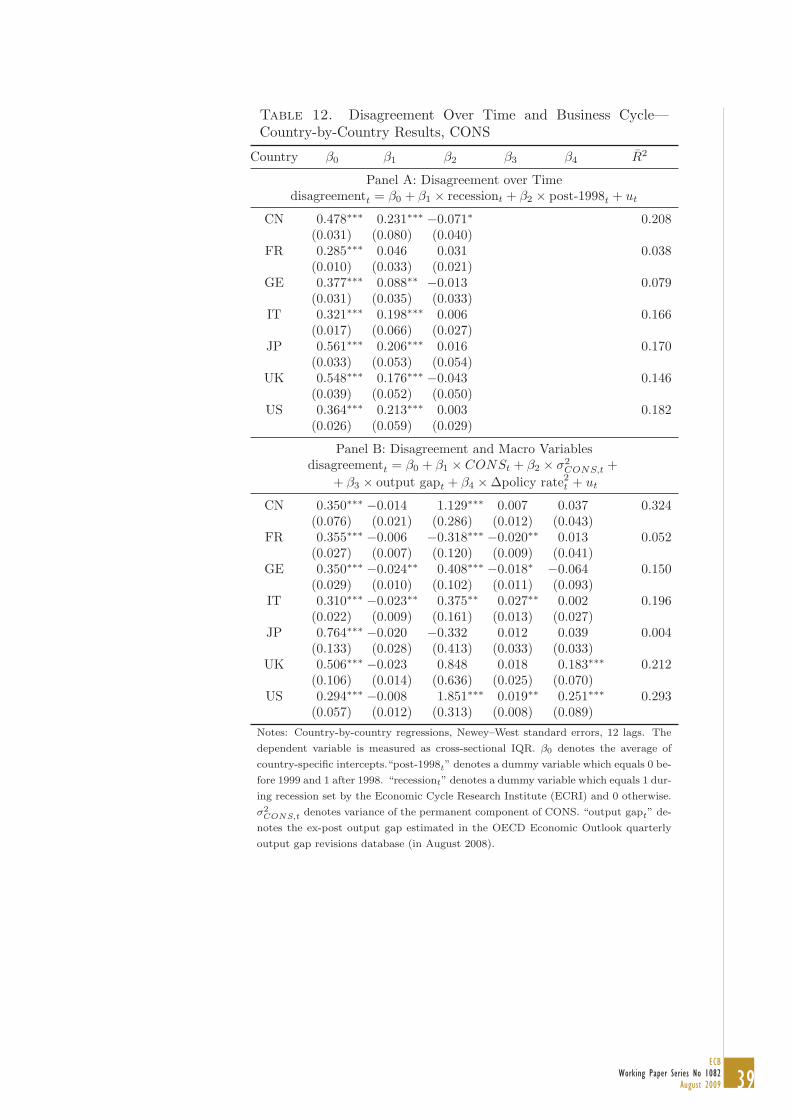
39ECB
Working Paper Series No 1082August 2009
Table 12. Disagreement Over Time and Business Cycle—Country-by-Country Results, CONS
Country β0 β1 β2 β3 β4 R2
Panel A: Disagreement over Timedisagreementt = β0 + β1 × recessiont + β2 × post-1998t + ut
CN 0.478∗∗∗ 0.231∗∗∗ −0.071∗ 0.208(0.031) (0.080) (0.040)
FR 0.285∗∗∗ 0.046 0.031 0.038(0.010) (0.033) (0.021)
GE 0.377∗∗∗ 0.088∗∗ −0.013 0.079(0.031) (0.035) (0.033)
IT 0.321∗∗∗ 0.198∗∗∗ 0.006 0.166(0.017) (0.066) (0.027)
JP 0.561∗∗∗ 0.206∗∗∗ 0.016 0.170(0.033) (0.053) (0.054)
UK 0.548∗∗∗ 0.176∗∗∗ −0.043 0.146(0.039) (0.052) (0.050)
US 0.364∗∗∗ 0.213∗∗∗ 0.003 0.182(0.026) (0.059) (0.029)
Panel B: Disagreement and Macro Variablesdisagreementt = β0 + β1 × CONSt + β2 × σ2
CONS,t ++ β3 × output gapt + β4 ×Δpolicy rate2
t + ut
CN 0.350∗∗∗ −0.014 1.129∗∗∗ 0.007 0.037 0.324(0.076) (0.021) (0.286) (0.012) (0.043)
FR 0.355∗∗∗ −0.006 −0.318∗∗∗ −0.020∗∗ 0.013 0.052(0.027) (0.007) (0.120) (0.009) (0.041)
GE 0.350∗∗∗ −0.024∗∗ 0.408∗∗∗ −0.018∗ −0.064 0.150(0.029) (0.010) (0.102) (0.011) (0.093)
IT 0.310∗∗∗ −0.023∗∗ 0.375∗∗ 0.027∗∗ 0.002 0.196(0.022) (0.009) (0.161) (0.013) (0.027)
JP 0.764∗∗∗ −0.020 −0.332 0.012 0.039 0.004(0.133) (0.028) (0.413) (0.033) (0.033)
UK 0.506∗∗∗ −0.023 0.848 0.018 0.183∗∗∗ 0.212(0.106) (0.014) (0.636) (0.025) (0.070)
US 0.294∗∗∗ −0.008 1.851∗∗∗ 0.019∗∗ 0.251∗∗∗ 0.293(0.057) (0.012) (0.313) (0.008) (0.089)
Notes: Country-by-country regressions, Newey–West standard errors, 12 lags. The
dependent variable is measured as cross-sectional IQR. β0 denotes the average of
country-specific intercepts.“post-1998t” denotes a dummy variable which equals 0 be-
fore 1999 and 1 after 1998. “recessiont” denotes a dummy variable which equals 1 dur-
ing recession set by the Economic Cycle Research Institute (ECRI) and 0 otherwise.
σ2CONS,t denotes variance of the permanent component of CONS. “output gapt” de-
notes the ex-post output gap estimated in the OECD Economic Outlook quarterly
output gap revisions database (in August 2008).

40ECBWorking Paper Series No 1082August 2009
Table 13. Disagreement Over Time and Business Cycle—Country-by-Country Results, INV
Country β0 β1 β2 β3 β4 R2
Panel A: Disagreement over Timedisagreementt = β0 + β1 × recessiont + β2 × post-1998t + ut
CN 2.929∗∗∗ −0.369∗ −0.619∗∗ 0.083(0.150) (0.192) (0.248)
FR 1.170∗∗∗ 0.001 −0.004 −0.010(0.037) (0.093) (0.100)
GE 1.284∗∗∗ 0.293∗∗ 0.374∗∗∗ 0.201(0.104) (0.119) (0.112)
IT 1.027∗∗∗ 0.224 −0.085 0.024(0.117) (0.142) (0.183)
JP 2.141∗∗∗ 0.294 0.346 0.061(0.165) (0.296) (0.271)
UK 1.641∗∗∗ 0.727∗∗∗ −0.147 0.224(0.114) (0.178) (0.149)
US 1.845∗∗∗ 1.021∗∗∗ −0.003 0.217(0.097) (0.117) (0.138)
Panel B: Disagreement and Macro Variablesdisagreementt = β0 + β1 × INVt + β2 × σ2
INV,t ++ β3 × output gapt + β4 ×Δpolicy rate2
t + ut
CN 1.646∗∗∗ 0.017 0.580∗∗∗ 0.179∗ 0.125 0.170(0.252) (0.020) (0.162) (0.093) (0.177)
FR 1.244∗∗∗ −0.026∗ −0.047 0.034 0.050 0.037(0.100) (0.014) (0.161) (0.043) (0.238)
GE 1.745∗∗∗ −0.029∗ −0.079 0.047 0.032 0.061(0.119) (0.016) (0.091) (0.035) (0.513)
IT 0.661∗∗∗ −0.039∗∗∗ 0.362∗∗∗ 0.171∗∗∗ 0.004 0.217(0.124) (0.015) (0.088) (0.059) (0.087)
JP 2.227∗∗∗ 0.059 0.032 −0.188∗∗∗ −1.426 0.110(0.352) (0.038) (0.491) (0.071) (0.931)
UK 1.725∗∗∗ −0.047∗∗∗ 0.017 0.051 0.309 0.228(0.182) (0.011) (0.118) (0.050) (0.294)
US 1.825∗∗∗ −0.030 0.365 −0.001 0.968 0.168(0.264) (0.023) (0.273) (0.054) (0.630)
Notes: Country-by-country regressions, Newey–West standard errors, 12 lags. The
dependent variable is measured as cross-sectional IQR. β0 denotes the average of
country-specific intercepts.“post-1998t” denotes a dummy variable which equals 0
before 1999 and 1 after 1998. “recessiont” denotes a dummy variable which equals
1 during recession set by the Economic Cycle Research Institute (ECRI) and 0 oth-
erwise. σ2INV,t denotes variance of the permanent component of INV. “output gapt”
denotes the ex-post output gap estimated in the OECD Economic Outlook quarterly
output gap revisions database (in August 2008).
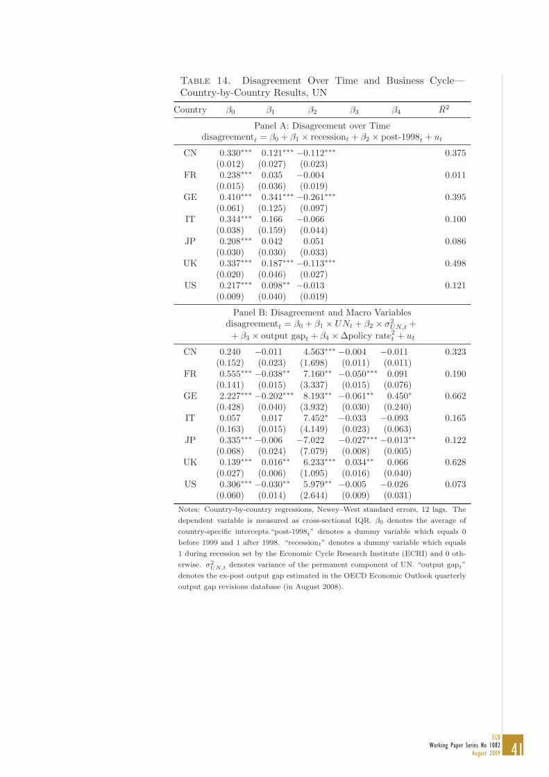
41ECB
Working Paper Series No 1082August 2009
Table 14. Disagreement Over Time and Business Cycle—Country-by-Country Results, UN
Country β0 β1 β2 β3 β4 R2
Panel A: Disagreement over Timedisagreementt = β0 + β1 × recessiont + β2 × post-1998t + ut
CN 0.330∗∗∗ 0.121∗∗∗ −0.112∗∗∗ 0.375(0.012) (0.027) (0.023)
FR 0.238∗∗∗ 0.035 −0.004 0.011(0.015) (0.036) (0.019)
GE 0.410∗∗∗ 0.341∗∗∗ −0.261∗∗∗ 0.395(0.061) (0.125) (0.097)
IT 0.344∗∗∗ 0.166 −0.066 0.100(0.038) (0.159) (0.044)
JP 0.208∗∗∗ 0.042 0.051 0.086(0.030) (0.030) (0.033)
UK 0.337∗∗∗ 0.187∗∗∗ −0.113∗∗∗ 0.498(0.020) (0.046) (0.027)
US 0.217∗∗∗ 0.098∗∗ −0.013 0.121(0.009) (0.040) (0.019)
Panel B: Disagreement and Macro Variablesdisagreementt = β0 + β1 × UNt + β2 × σ2
UN,t ++ β3 × output gapt + β4 ×Δpolicy rate2
t + ut
CN 0.240 −0.011 4.563∗∗∗ −0.004 −0.011 0.323(0.152) (0.023) (1.698) (0.011) (0.011)
FR 0.555∗∗∗ −0.038∗∗ 7.160∗∗ −0.050∗∗∗ 0.091 0.190(0.141) (0.015) (3.337) (0.015) (0.076)
GE 2.227∗∗∗ −0.202∗∗∗ 8.193∗∗ −0.061∗∗ 0.450∗ 0.662(0.428) (0.040) (3.932) (0.030) (0.240)
IT 0.057 0.017 7.452∗ −0.033 −0.093 0.165(0.163) (0.015) (4.149) (0.023) (0.063)
JP 0.335∗∗∗ −0.006 −7.022 −0.027∗∗∗ −0.013∗∗ 0.122(0.068) (0.024) (7.079) (0.008) (0.005)
UK 0.139∗∗∗ 0.016∗∗ 6.233∗∗∗ 0.034∗∗ 0.066 0.628(0.027) (0.006) (1.095) (0.016) (0.040)
US 0.306∗∗∗ −0.030∗∗ 5.979∗∗ −0.005 −0.026 0.073(0.060) (0.014) (2.644) (0.009) (0.031)
Notes: Country-by-country regressions, Newey–West standard errors, 12 lags. The
dependent variable is measured as cross-sectional IQR. β0 denotes the average of
country-specific intercepts.“post-1998t” denotes a dummy variable which equals 0
before 1999 and 1 after 1998. “recessiont” denotes a dummy variable which equals
1 during recession set by the Economic Cycle Research Institute (ECRI) and 0 oth-
erwise. σ2UN,t denotes variance of the permanent component of UN. “output gapt”
denotes the ex-post output gap estimated in the OECD Economic Outlook quarterly
output gap revisions database (in August 2008).

42ECBWorking Paper Series No 1082August 2009
Appendix—Additional Results
Table 15. Correlation between the Two Disagreement Mea-sures (Cross-Sectional IQR and Standard Deviation)
Canada France Germany Italy Japan UK US
Inflation 0.75 0.61 0.58 0.82 0.68 0.92 0.70Interest Rate 0.87 0.78 0.80 0.84 0.88 0.86 0.73GDP 0.79 0.62 0.78 0.69 0.76 0.66 0.83Consumption 0.78 0.51 0.69 0.68 0.76 0.72 0.82Investment 0.72 0.67 0.77 0.80 0.78 0.71 0.75Unemployment 0.79 0.66 0.93 0.84 0.75 0.85 0.71
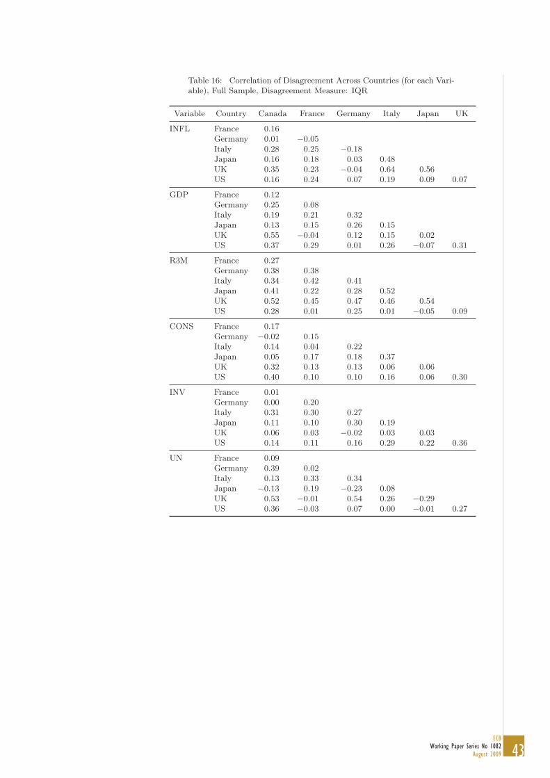
43ECB
Working Paper Series No 1082August 2009
Table 16: Correlation of Disagreement Across Countries (for each Vari-able), Full Sample, Disagreement Measure: IQR
Variable Country Canada France Germany Italy Japan UK
INFL France 0.16Germany 0.01 −0.05Italy 0.28 0.25 −0.18Japan 0.16 0.18 0.03 0.48UK 0.35 0.23 −0.04 0.64 0.56US 0.16 0.24 0.07 0.19 0.09 0.07
GDP France 0.12Germany 0.25 0.08Italy 0.19 0.21 0.32Japan 0.13 0.15 0.26 0.15UK 0.55 −0.04 0.12 0.15 0.02US 0.37 0.29 0.01 0.26 −0.07 0.31
R3M France 0.27Germany 0.38 0.38Italy 0.34 0.42 0.41Japan 0.41 0.22 0.28 0.52UK 0.52 0.45 0.47 0.46 0.54US 0.28 0.01 0.25 0.01 −0.05 0.09
CONS France 0.17Germany −0.02 0.15Italy 0.14 0.04 0.22Japan 0.05 0.17 0.18 0.37UK 0.32 0.13 0.13 0.06 0.06US 0.40 0.10 0.10 0.16 0.06 0.30
INV France 0.01Germany 0.00 0.20Italy 0.31 0.30 0.27Japan 0.11 0.10 0.30 0.19UK 0.06 0.03 −0.02 0.03 0.03US 0.14 0.11 0.16 0.29 0.22 0.36
UN France 0.09Germany 0.39 0.02Italy 0.13 0.33 0.34Japan −0.13 0.19 −0.23 0.08UK 0.53 −0.01 0.54 0.26 −0.29US 0.36 −0.03 0.07 0.00 −0.01 0.27

44ECBWorking Paper Series No 1082August 2009
Table 17: Correlation of Disagreement Across Variables Within Coun-try, Full Sample, Disagreement Measure: IQR
Country Variable Inflation GDP Int. Rate Cons Inv
CN GDP 0.19Interest Rate 0.22 0.27Consumption 0.22 0.53 0.27Investment 0.11 0.25 0.05 0.15Unemployment 0.31 0.57 0.34 0.48 0.28
FR GDP 0.16Interest Rate 0.26 0.14Consumption 0.04 0.41 0.12Investment 0.20 0.39 0.19 0.28Unemployment 0.05 0.23 0.27 0.16 0.11
GE GDP −0.03Interest Rate 0.09 0.18Consumption 0.14 0.44 0.28Investment 0.07 0.17 0.11 0.32Unemployment −0.04 0.34 0.22 0.23 −0.08
IT GDP 0.17Interest Rate 0.56 0.12Consumption 0.25 0.39 0.16Investment 0.29 0.36 0.23 0.32Unemployment 0.31 0.32 0.12 0.32 0.26
JP GDP 0.26Interest Rate 0.47 0.06Consumption 0.24 0.57 0.08Investment 0.13 0.53 −0.03 0.38Unemployment 0.04 0.50 −0.14 0.39 0.26
UK GDP 0.49Interest Rate 0.66 0.53Consumption 0.31 0.59 0.33Investment 0.37 0.56 0.41 0.52Unemployment 0.47 0.63 0.61 0.45 0.56
US GDP 0.41Interest Rate 0.31 0.22Consumption 0.36 0.74 0.05Investment 0.32 0.55 0.11 0.50Unemployment 0.18 0.48 0.12 0.50 0.37

45ECB
Working Paper Series No 1082August 2009
DISAGREEMENT AMONG FORECASTERS 39Fig
ure
1.
Exp
ecte
dan
dA
ctua
lIn
flati
onR
ate
(Per
cent
)
−202468
1990
1995
2000
2005
CN
0123451990
1995
2000
2005
FR
02468
1990
1995
2000
2005
GE
02468
1990
1995
2000
2005
IT
−4−20246
1990
1995
2000
2005
JP
0510
1990
1995
2000
2005
UK
02468
1990
1995
2000
2005
US
Note
:Shaded
are
as
den
ote
rece
ssio
ns
as
iden
tified
by
the
Eco
nom
icC
ycl
eR
esea
rch
Inst
itute
(usi
ng
the
busi
nes
scy
cle
met
hod).

46ECBWorking Paper Series No 1082August 2009
40 DOVERN, FRITSCHE AND SLACALEKFig
ure
2.
Exp
ecte
dan
dA
ctua
lSh
ort-
term
Inte
rest
Rat
es(P
erce
nt)
051015
1990
1995
2000
2005
CN
051015
1990
1995
2000
2005
FR
0246810
1990
1995
2000
2005
GE
05101520
1990
1995
2000
2005
IT0246810
1990
1995
2000
2005
JP
051015
1990
1995
2000
2005
UK
0246810
1990
1995
2000
2005
US
Note
:Shaded
are
as
den
ote
rece
ssio
ns
as
iden
tified
by
the
Eco
nom
icC
ycl
eR
esea
rch
Inst
itute
(usi
ng
the
busi
nes
scy
cle
met
hod).
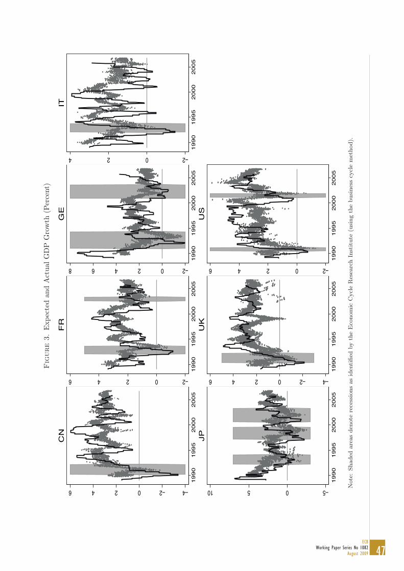
47ECB
Working Paper Series No 1082August 2009
DISAGREEMENT AMONG FORECASTERS 41Fig
ure
3.
Exp
ecte
dan
dA
ctua
lG
DP
Gro
wth
(Per
cent
)
−4−20246
1990
1995
2000
2005
CN
−202461990
1995
2000
2005
FR
−202468
1990
1995
2000
2005
GE
−2024
1990
1995
2000
2005
IT
−50510
1990
1995
2000
2005
JP
−4−20246
1990
1995
2000
2005
UK
−20246
1990
1995
2000
2005
US
Note
:Shaded
are
as
den
ote
rece
ssio
ns
as
iden
tified
by
the
Eco
nom
icC
ycl
eR
esea
rch
Inst
itute
(usi
ng
the
busi
nes
scy
cle
met
hod).
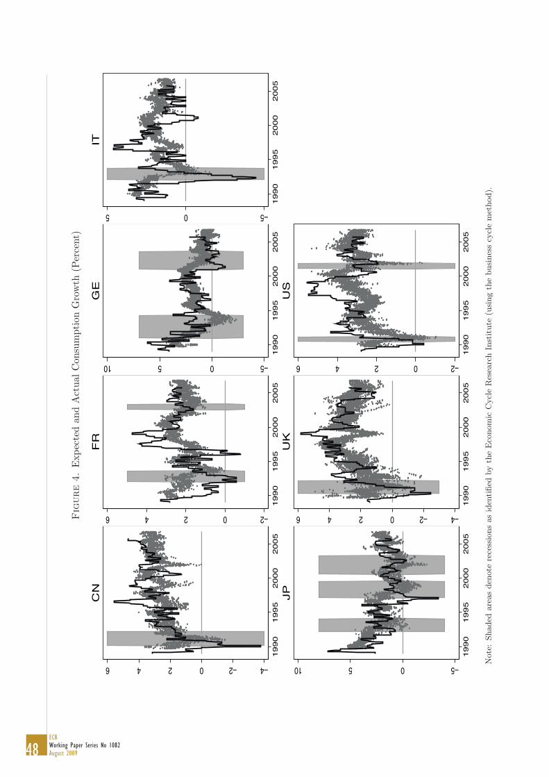
48ECBWorking Paper Series No 1082August 2009
42 DOVERN, FRITSCHE AND SLACALEKFig
ure
4.
Exp
ecte
dan
dA
ctua
lC
onsu
mpt
ion
Gro
wth
(Per
cent
)
−4−20246
1990
1995
2000
2005
CN
−20246
1990
1995
2000
2005
FR
−50510
1990
1995
2000
2005
GE
−505
1990
1995
2000
2005
IT−50510
1990
1995
2000
2005
JP
−4−20246
1990
1995
2000
2005
UK
−20246
1990
1995
2000
2005
US
Note
:Shaded
are
as
den
ote
rece
ssio
ns
as
iden
tified
by
the
Eco
nom
icC
ycl
eR
esea
rch
Inst
itute
(usi
ng
the
busi
nes
scy
cle
met
hod).

49ECB
Working Paper Series No 1082August 2009
DISAGREEMENT AMONG FORECASTERS 43Fig
ure
5.
Exp
ecte
dan
dA
ctua
lIn
vest
men
tG
row
th(P
erce
nt)
−1001020
1990
1995
2000
2005
CN
−505101990
1995
2000
2005
FR
−10−5051015
1990
1995
2000
2005
GE
−15−10−50510
1990
1995
2000
2005
IT
−20−1001020
1990
1995
2000
2005
JP
−10−5051015
1990
1995
2000
2005
UK
−20−1001020
1990
1995
2000
2005
US
Note
:Shaded
are
as
den
ote
rece
ssio
ns
as
iden
tified
by
the
Eco
nom
icC
ycl
eR
esea
rch
Inst
itute
(usi
ng
the
busi
nes
scy
cle
met
hod).

50ECBWorking Paper Series No 1082August 2009
44 DOVERN, FRITSCHE AND SLACALEKFig
ure
6.
Exp
ecte
dan
dA
ctua
lU
nem
ploy
men
tR
ate
(Per
cent
)
051015
1990
1995
2000
2005
CN
051015
1990
1995
2000
2005
FR
051015
1990
1995
2000
2005
GE
051015
1990
1995
2000
2005
IT02468
1990
1995
2000
2005
JP
051015
1990
1995
2000
2005
UK
02468
1990
1995
2000
2005
US
Note
:Shaded
are
as
den
ote
rece
ssio
ns
as
iden
tified
by
the
Eco
nom
icC
ycl
eR
esea
rch
Inst
itute
(usi
ng
the
busi
nes
scy
cle
met
hod).
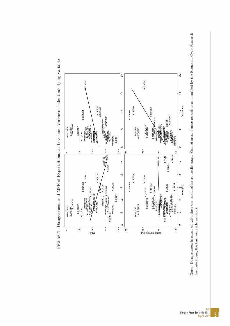
51ECB
Working Paper Series No 1082August 2009
Fig
ure
7.
Dis
agre
emen
tan
dM
SEof
Exp
ecta
tion
svs
.Lev
elan
dV
aria
nce
ofth
eU
nder
lyin
gV
aria
ble
CN
INFL
FRIN
FL
GE
INFL
ITIN
FLJP
INFL
UK
INFL
US
INFL
CN
GD
P
FRG
DP
GE
GD
P
ITG
DP
JPG
DP UK
GD
P
US
GD
PC
NR
3M
FRR
3M
GE
R3M
ITR
3M
JPR
3M
UK
R3M
US
R3M
CN
CO
NS
FRC
ON
S
GE
CO
NS
ITC
ON
S
JPC
ON
S
UK
CO
NS
US
CO
NS
CN
UN
FRU
NG
EU
NIT
UN
JPU
N
UK
UN
US
UN
01234MSE
02
46
810
CN
INFL
FRIN
FLGE
INFL
ITIN
FLJP
INFL
UK
INFL
US
INFL
CN
GD
P
FRG
DPG
EG
DP
ITG
DPJP
GD
P
UK
GD
P
US
GD
PC
NR
3M
FRR
3M
GE
R3M
ITR
3M
JPR
3M
UK
R3M
US
R3M
CN
CO
NS
FRC
ON
S
GE
CO
NS
ITC
ON
S
JPC
ON
S
UK
CO
NS
US
CO
NS
CN
UN
FRU
NGE
UN
ITU
N
JPU
N
UK
UN
US
UN
01234
05
1015
20
CN
INFL
FRIN
FLG
EIN
FLIT
INFL
JPIN
FL
UK
INFL
US
INFL
CN
GD
P
FRG
DP
GE
GD
P
ITG
DP
JPG
DP UK
GD
P
US
GD
P
CN
R3M
FRR
3MG
ER
3M
ITR
3M
JPR
3M
UK
R3M
US
R3M
CN
CO
NS
FRC
ON
S
GE
CO
NS
ITC
ON
S
JPC
ON
S
UK
CO
NS
US
CO
NS
CN
UN
FRU
N
GE
UN
ITU
N
JPU
N
UK
UN
US
UN
.2.4.6.8Disagreement (%)
02
46
810
Leve
l (%
)
CN
INFL
FRIN
FLGE
INFL
ITIN
FL
JPIN
FL
UK
INFL
US
INFL
CN
GD
P
FRG
DPG
EG
DP
ITG
DPJP
GD
P
UK
GD
P
US
GD
P
CN
R3M
FRR
3MG
ER
3M
ITR
3M
JPR
3M
UK
R3M
US
R3M
CN
CO
NS
FRC
ON
S
GE
CO
NS
ITC
ON
S
JPC
ON
S
UK
CO
NS
US
CO
NS
CN
UN
FRU
NGE
UN
ITU
N
JPU
N
UK
UN
US
UN
.2.4.6.8
05
1015
20V
aria
nce
Note
s:D
isagre
emen
tis
mea
sure
dw
ith
the
cross
-sec
tionalin
terq
uart
ile
range.
Shaded
are
as
den
ote
rece
ssio
ns
as
iden
tified
by
the
Eco
nom
icC
ycl
eR
esea
rch
Inst
itute
(usi
ng
the
busi
nes
scy
cle
met
hod).
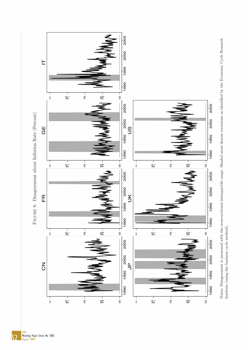
52ECBWorking Paper Series No 1082August 2009
46 DOVERN, FRITSCHE AND SLACALEKFig
ure
8.
Dis
agre
emen
tab
out
Infla
tion
Rat
e(P
erce
nt)
0.25.5.751
1990
1995
2000
2005
CN
0.25.5.751
1990
1995
2000
2005
FR
0.25.5.751
1990
1995
2000
2005
GE
0.25.5.751
1990
1995
2000
2005
IT0.25.5.751
1990
1995
2000
2005
JP
0.25.5.751
1990
1995
2000
2005
UK
0.25.5.751
1990
1995
2000
2005
US
Note
s:D
isagre
emen
tis
mea
sure
dw
ith
the
cross
-sec
tionalin
terq
uart
ile
range.
Shaded
are
as
den
ote
rece
ssio
ns
as
iden
tified
by
the
Eco
nom
icC
ycl
eR
esea
rch
Inst
itute
(usi
ng
the
busi
nes
scy
cle
met
hod).

53ECB
Working Paper Series No 1082August 2009
DISAGREEMENT AMONG FORECASTERS 47
Fig
ure
9.
Dis
agre
emen
tab
out
Shor
t-te
rmIn
tere
stR
ate
(Per
cent
)
0.25.5.7511.251.51.752
1990
1995
2000
2005
CN
0.25.5.7511.251.51.7521990
1995
2000
2005
FR
0.25.5.7511.251.51.752
1990
1995
2000
2005
GE
0.25.5.7511.251.51.752
1990
1995
2000
2005
IT
0.25.5.7511.251.51.752
1990
1995
2000
2005
JP0.25.5.7511.251.51.752
1990
1995
2000
2005
UK
0.25.5.7511.251.51.752
1990
1995
2000
2005
US
Note
s:D
isagre
emen
tis
mea
sure
dw
ith
the
cross
-sec
tionalin
terq
uart
ile
range.
Shaded
are
as
den
ote
rece
ssio
ns
as
iden
tified
by
the
Eco
nom
icC
ycl
eR
esea
rch
Inst
itute
(usi
ng
the
busi
nes
scy
cle
met
hod).
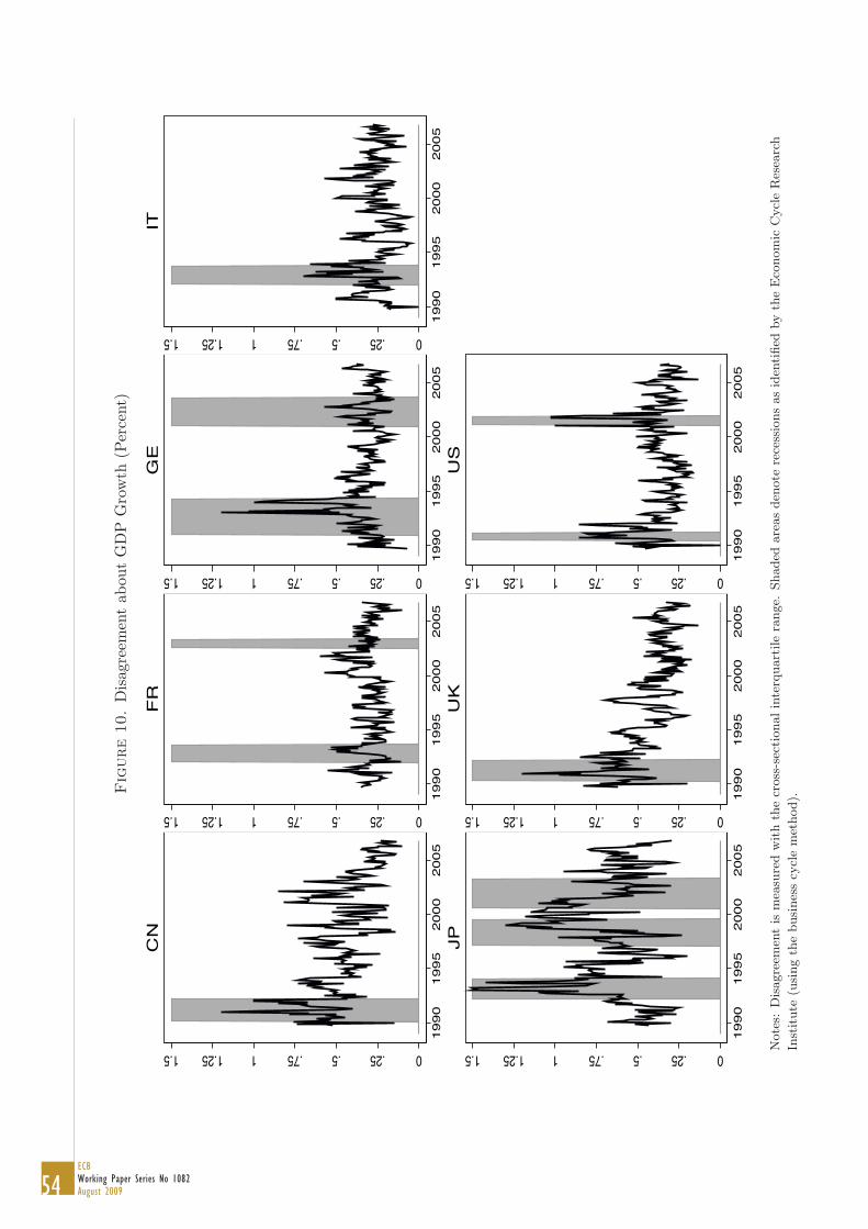
54ECBWorking Paper Series No 1082August 2009
48 DOVERN, FRITSCHE AND SLACALEKFig
ure
10.
Dis
agre
emen
tab
out
GD
PG
row
th(P
erce
nt)
0.25.5.7511.251.5
1990
1995
2000
2005
CN
0.25.5.7511.251.5
1990
1995
2000
2005
FR
0.25.5.7511.251.5
1990
1995
2000
2005
GE
0.25.5.7511.251.5
1990
1995
2000
2005
IT0.25.5.7511.251.5
1990
1995
2000
2005
JP
0.25.5.7511.251.5
1990
1995
2000
2005
UK
0.25.5.7511.251.5
1990
1995
2000
2005
US
Note
s:D
isagre
emen
tis
mea
sure
dw
ith
the
cross
-sec
tionalin
terq
uart
ile
range.
Shaded
are
as
den
ote
rece
ssio
ns
as
iden
tified
by
the
Eco
nom
icC
ycl
eR
esea
rch
Inst
itute
(usi
ng
the
busi
nes
scy
cle
met
hod).
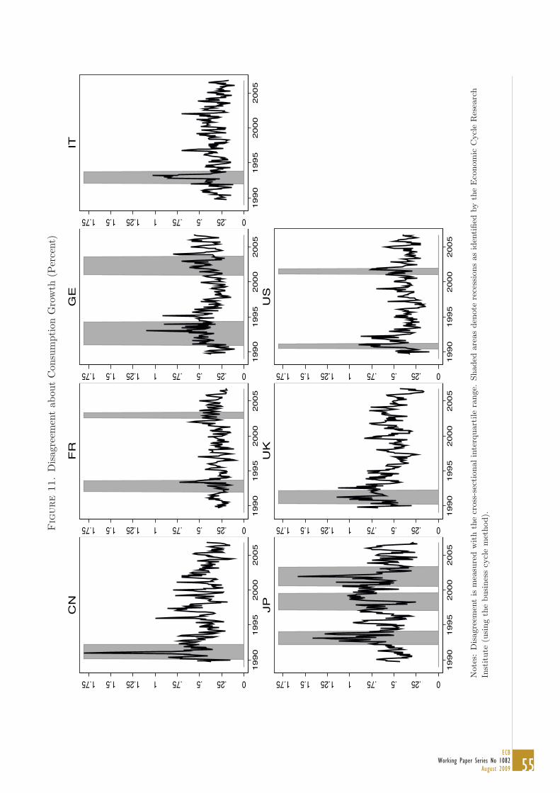
55ECB
Working Paper Series No 1082August 2009
DISAGREEMENT AMONG FORECASTERS 49
Fig
ure
11.
Dis
agre
emen
tab
out
Con
sum
ptio
nG
row
th(P
erce
nt)
0.25.5.7511.251.51.75
1990
1995
2000
2005
CN
0.25.5.7511.251.51.751990
1995
2000
2005
FR
0.25.5.7511.251.51.75
1990
1995
2000
2005
GE
0.25.5.7511.251.51.75
1990
1995
2000
2005
IT
0.25.5.7511.251.51.75
1990
1995
2000
2005
JP0.25.5.7511.251.51.75
1990
1995
2000
2005
UK
0.25.5.7511.251.51.75
1990
1995
2000
2005
US
Note
s:D
isagre
emen
tis
mea
sure
dw
ith
the
cross
-sec
tionalin
terq
uart
ile
range.
Shaded
are
as
den
ote
rece
ssio
ns
as
iden
tified
by
the
Eco
nom
icC
ycl
eR
esea
rch
Inst
itute
(usi
ng
the
busi
nes
scy
cle
met
hod).

56ECBWorking Paper Series No 1082August 2009
50 DOVERN, FRITSCHE AND SLACALEKFig
ure
12.
Dis
agre
emen
tab
out
Inve
stm
ent
Gro
wth
(Per
cent
)
0.511.522.533.544.555.56
1990
1995
2000
2005
CN
0.511.522.533.544.555.56
1990
1995
2000
2005
FR
0.511.522.533.544.555.56
1990
1995
2000
2005
GE
0.511.522.533.544.555.56
1990
1995
2000
2005
IT0.511.522.533.544.555.56
1990
1995
2000
2005
JP
0.511.522.533.544.555.56
1990
1995
2000
2005
UK
0.511.522.533.544.555.56
1990
1995
2000
2005
US
Note
s:D
isagre
emen
tis
mea
sure
dw
ith
the
cross
-sec
tionalin
terq
uart
ile
range.
Shaded
are
as
den
ote
rece
ssio
ns
as
iden
tified
by
the
Eco
nom
icC
ycl
eR
esea
rch
Inst
itute
(usi
ng
the
busi
nes
scy
cle
met
hod).
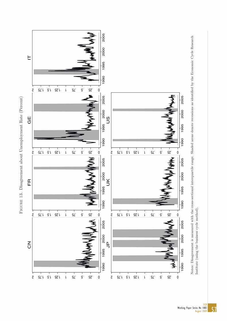
57ECB
Working Paper Series No 1082August 2009
DISAGREEMENT AMONG FORECASTERS 51
Fig
ure
13.
Dis
agre
emen
tab
out
Une
mpl
oym
ent
Rat
e(P
erce
nt)
0.25.5.7511.251.51.752
1990
1995
2000
2005
CN
0.25.5.7511.251.51.7521990
1995
2000
2005
FR
0.25.5.7511.251.51.752
1990
1995
2000
2005
GE
0.25.5.7511.251.51.752
1990
1995
2000
2005
IT
0.25.5.7511.251.51.752
1990
1995
2000
2005
JP0.25.5.7511.251.51.752
1990
1995
2000
2005
UK
0.25.5.7511.251.51.752
1990
1995
2000
2005
US
Note
s:D
isagre
emen
tis
mea
sure
dw
ith
the
cross
-sec
tionalin
terq
uart
ile
range.
Shaded
are
as
den
ote
rece
ssio
ns
as
iden
tified
by
the
Eco
nom
icC
ycl
eR
esea
rch
Inst
itute
(usi
ng
the
busi
nes
scy
cle
met
hod).

58ECBWorking Paper Series No 1082August 2009
52 DOVERN, FRITSCHE AND SLACALEKFig
ure
14.
Var
ianc
eof
Per
man
ent
Com
pone
ntσ
2 ε,t—
Infla
tion
0.1.2.3.4
1990
1995
2000
2005
CN
0.1.2.3.4
1990
1995
2000
2005
FR
0.1.2.3.4
1990
1995
2000
2005
GE
0.1.2.3.4
1990
1995
2000
2005
IT0.1.2.3.4
1990
1995
2000
2005
JP
0.1.2.3.4
1990
1995
2000
2005
UK
0.1.2.3.4
1990
1995
2000
2005
US
Note
:Shaded
are
as
den
ote
rece
ssio
ns
as
iden
tified
by
the
Eco
nom
icC
ycl
eR
esea
rch
Inst
itute
(usi
ng
the
busi
nes
scy
cle
met
hod).

59ECB
Working Paper Series No 1082August 2009
DISAGREEMENT AMONG FORECASTERS 53Fig
ure
15.
Var
ianc
eof
Per
man
ent
Com
pone
ntσ
2 ε,t—
Inte
rest
Rat
e
0.2.4.6.81
1990
1995
2000
2005
CN
0.2.4.6.811990
1995
2000
2005
FR
0.2.4.6.81
1990
1995
2000
2005
GE
0.2.4.6.81
1990
1995
2000
2005
IT
0.2.4.6.81
1990
1995
2000
2005
JP0.2.4.6.81
1990
1995
2000
2005
UK
0.2.4.6.81
1990
1995
2000
2005
US
Note
:Shaded
are
as
den
ote
rece
ssio
ns
as
iden
tified
by
the
Eco
nom
icC
ycl
eR
esea
rch
Inst
itute
(usi
ng
the
busi
nes
scy
cle
met
hod).
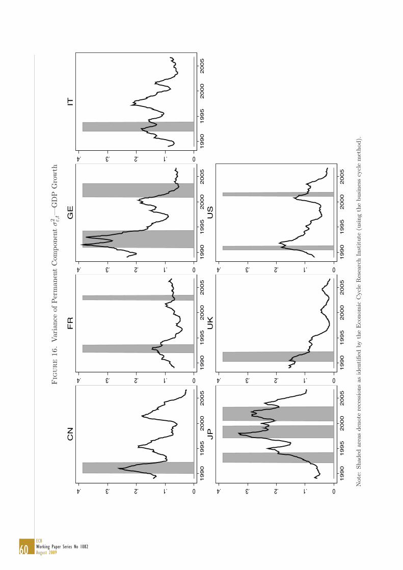
60ECBWorking Paper Series No 1082August 2009
54 DOVERN, FRITSCHE AND SLACALEKFig
ure
16.
Var
ianc
eof
Per
man
ent
Com
pone
ntσ
2 ε,t—
GD
PG
row
th
0.1.2.3.4
1990
1995
2000
2005
CN
0.1.2.3.4
1990
1995
2000
2005
FR
0.1.2.3.4
1990
1995
2000
2005
GE
0.1.2.3.4
1990
1995
2000
2005
IT0.1.2.3.4
1990
1995
2000
2005
JP
0.1.2.3.4
1990
1995
2000
2005
UK
0.1.2.3.4
1990
1995
2000
2005
US
Note
:Shaded
are
as
den
ote
rece
ssio
ns
as
iden
tified
by
the
Eco
nom
icC
ycl
eR
esea
rch
Inst
itute
(usi
ng
the
busi
nes
scy
cle
met
hod).
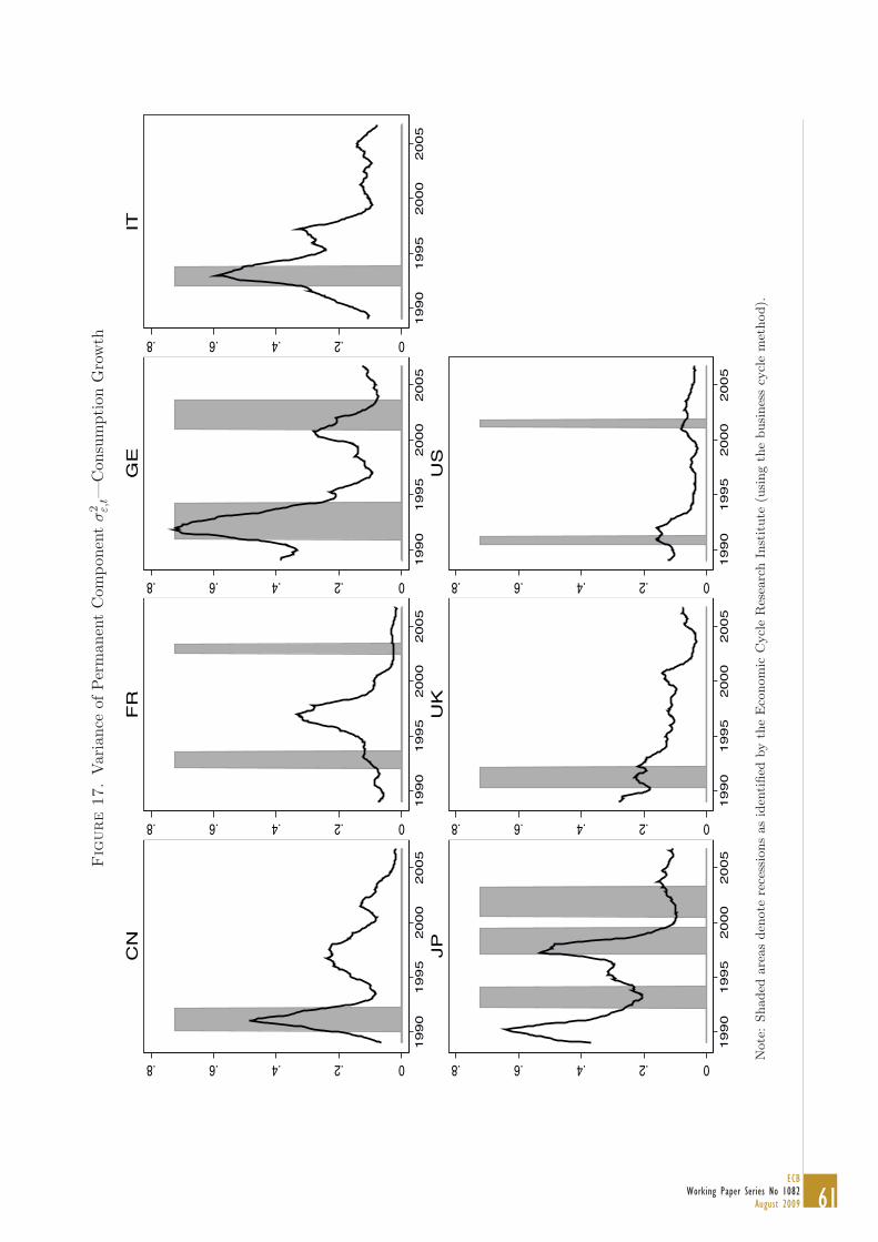
61ECB
Working Paper Series No 1082August 2009
DISAGREEMENT AMONG FORECASTERS 55Fig
ure
17.
Var
ianc
eof
Per
man
ent
Com
pone
ntσ
2 ε,t—
Con
sum
ptio
nG
row
th
0.2.4.6.8
1990
1995
2000
2005
CN
0.2.4.6.81990
1995
2000
2005
FR
0.2.4.6.8
1990
1995
2000
2005
GE
0.2.4.6.8
1990
1995
2000
2005
IT
0.2.4.6.8
1990
1995
2000
2005
JP0.2.4.6.8
1990
1995
2000
2005
UK
0.2.4.6.8
1990
1995
2000
2005
US
Note
:Shaded
are
as
den
ote
rece
ssio
ns
as
iden
tified
by
the
Eco
nom
icC
ycl
eR
esea
rch
Inst
itute
(usi
ng
the
busi
nes
scy
cle
met
hod).
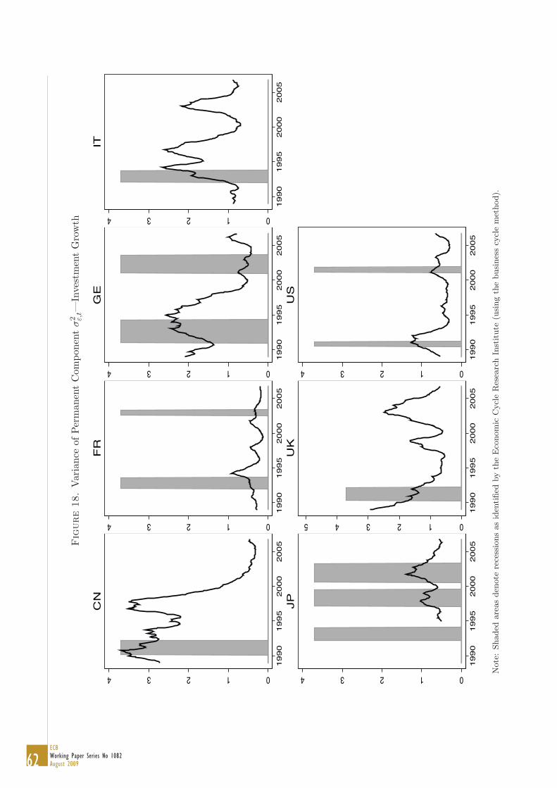
62ECBWorking Paper Series No 1082August 2009
56 DOVERN, FRITSCHE AND SLACALEKFig
ure
18.
Var
ianc
eof
Per
man
ent
Com
pone
ntσ
2 ε,t—
Inve
stm
ent
Gro
wth
01234
1990
1995
2000
2005
CN
01234
1990
1995
2000
2005
FR
01234
1990
1995
2000
2005
GE
01234
1990
1995
2000
2005
IT01234
1990
1995
2000
2005
JP
012345
1990
1995
2000
2005
UK
01234
1990
1995
2000
2005
US
Note
:Shaded
are
as
den
ote
rece
ssio
ns
as
iden
tified
by
the
Eco
nom
icC
ycl
eR
esea
rch
Inst
itute
(usi
ng
the
busi
nes
scy
cle
met
hod).

63ECB
Working Paper Series No 1082August 2009
DISAGREEMENT AMONG FORECASTERS 57
Fig
ure
19.
Var
ianc
eof
Per
man
ent
Com
pone
ntσ
2 ε,t—
Une
mpl
oym
ent
Rat
e
0.02.04.06.08.1
1990
1995
2000
2005
CN
0.02.04.06.08.11990
1995
2000
2005
FR
0.02.04.06.08.1
1990
1995
2000
2005
GE
0.02.04.06.08.1
1990
1995
2000
2005
IT
0.02.04.06.08.1
1990
1995
2000
2005
JP0.02.04.06.08.1
1990
1995
2000
2005
UK
0.02.04.06.08.1
1990
1995
2000
2005
US
Note
:Shaded
are
as
den
ote
rece
ssio
ns
as
iden
tified
by
the
Eco
nom
icC
ycl
eR
esea
rch
Inst
itute
(usi
ng
the
busi
nes
scy
cle
met
hod).
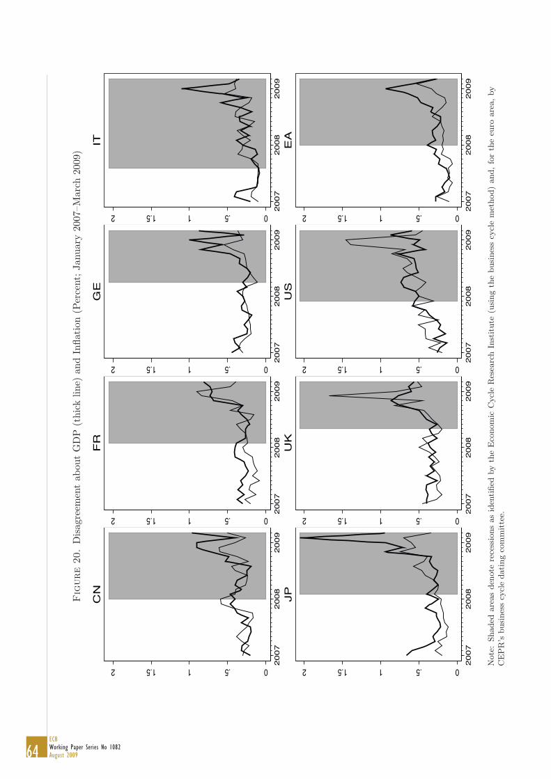
64ECBWorking Paper Series No 1082August 2009
Fig
ure
20.
Dis
agre
emen
tab
out
GD
P(t
hick
line)
and
Infla
tion
(Per
cent
;Ja
nuar
y20
07–M
arch
2009
)
0.511.52 2007
2008
2009
CN
0.511.52 2007
2008
2009
FR
0.511.52 2007
2008
2009
GE
0.511.52 2007
2008
2009
IT0.511.52 2
007
2008
2009
JP
0.511.52 2007
2008
2009
UK
0.511.52 2007
2008
2009
US
0.511.52 2007
2008
2009
EA
Note
:Shaded
are
as
den
ote
rece
ssio
ns
as
iden
tified
by
the
Eco
nom
icC
ycl
eR
esea
rch
Inst
itute
(usi
ng
the
busi
nes
scy
cle
met
hod)
and,fo
rth
eeu
roare
a,by
CE
PR
’sbusi
nes
scy
cle
dati
ng
com
mit
tee.

65ECB
Working Paper Series No 1082August 2009
Figure 21. Cross-sectional Dynamics of GDP and Inflation Ex-pectations (Percent; 2007–2009)—“Big” Economic Regions
01
23
45
−6 −5 −4 −3 −2 −1 0 1 2 3 4 5
EAGDP
02
46
−6 −5 −4 −3 −2 −1 0 1 2 3 4 5
EAINFL
0.5
11.5
2
−6 −5 −4 −3 −2 −1 0 1 2 3 4 5
USGDP
0.5
11
.5
−6 −5 −4 −3 −2 −1 0 1 2 3 4 5
USINFL
0.5
11.5
2
−6 −5 −4 −3 −2 −1 0 1 2 3 4 5
UKGDP
0.5
11.5
2
−6 −5 −4 −3 −2 −1 0 1 2 3 4 5
UKINFL
0.5
11.5
2
−6 −5 −4 −3 −2 −1 0 1 2 3 4 5
JPGDP
01
23
4
−6 −5 −4 −3 −2 −1 0 1 2 3 4 5
JPINFL
2007M6 2008M9 2008M10
2009M1 2009M2 2009M3
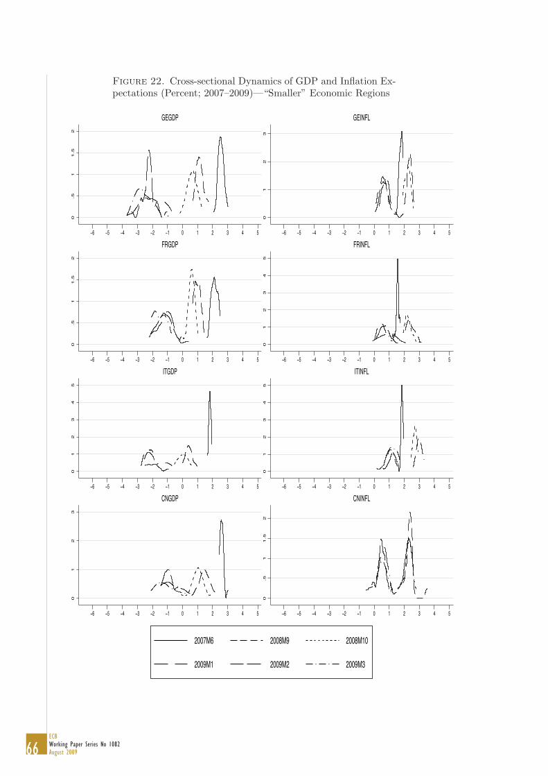
66ECBWorking Paper Series No 1082August 2009
Figure 22. Cross-sectional Dynamics of GDP and Inflation Ex-pectations (Percent; 2007–2009)—“Smaller” Economic Regions
0.5
11.5
2
−6 −5 −4 −3 −2 −1 0 1 2 3 4 5
GEGDP
01
23
−6 −5 −4 −3 −2 −1 0 1 2 3 4 5
GEINFL
0.5
11.5
2
−6 −5 −4 −3 −2 −1 0 1 2 3 4 5
FRGDP
01
23
45
−6 −5 −4 −3 −2 −1 0 1 2 3 4 5
FRINFL
01
23
45
−6 −5 −4 −3 −2 −1 0 1 2 3 4 5
ITGDP
01
23
45
−6 −5 −4 −3 −2 −1 0 1 2 3 4 5
ITINFL
01
23
−6 −5 −4 −3 −2 −1 0 1 2 3 4 5
CNGDP
0.5
11.5
2
−6 −5 −4 −3 −2 −1 0 1 2 3 4 5
CNINFL
2007M6 2008M9 2008M10
2009M1 2009M2 2009M3
67ECB
Working Paper Series No 1082August 2009
European Central Bank Working Paper Series
For a complete list of Working Papers published by the ECB, please visit the ECB’s website
(http://www.ecb.europa.eu).
1049 “Labour force participation in the euro area: a cohort based analysis” by A. Balleer, R. Gómez-Salvador
and J. Turunen, May 2009.
1050 “Wealth effects on consumption: evidence from the euro area” by R. M. Sousa, May 2009.
1051 “Are more data always better for factor analysis? Results for the euro area, the six largest euro area
countries and the UK” by G. Caggiano, G. Kapetanios and V. Labhard, May 2009.
1052 “Bidding behaviour in the ECB’s main refinancing operations during the financial crisis” by J. Eisenschmidt,
A. Hirsch and T. Linzert, May 2009.
1053 “Inflation dynamics with labour market matching: assessing alternative specifications” by K. Christoffel,
J. Costain, G. de Walque, K. Kuester, T. Linzert, S. Millard and O. Pierrard, May 2009.
1054 “Fiscal behaviour in the European Union: rules, fiscal decentralization and government indebtedness”
by A. Afonso and S. Hauptmeier, May 2009.
1055 “The impact of extreme weather events on budget balances and implications for fiscal policy”
by E. M. Lis and C. Nickel, May 2009.
1056 “The pricing of subprime mortgage risk in good times and bad: evidence from the ABX.HE indices”
by I. Fender and M. Scheicher, May 2009.
1057 “Euro area private consumption: Is there a role for housing wealth effects?” by F. Skudelny, May 2009.
1058 “National prices and wage setting in a currency union” by M. Sánchez, May 2009.
1059 “Forecasting the world economy in the short-term” by A. Jakaitiene and S. Dées, June 2009.
1060 “What explains global exchange rate movements during the financial crisis?” by M. Fratzscher, June 2009.
1061 “The distribution of households consumption-expenditure budget shares” by M. Barigozzi, L. Alessi,
M. Capasso and G. Fagiolo, June 2009.
1062 “External shocks and international inflation linkages: a global VAR analysis” by A. Galesi and M. J. Lombardi,
June 2009.
1063 “Does private equity investment spur innovation? Evidence from Europe” by A. Popov and P. Roosenboom,
June 2009.
1064 “Does it pay to have the euro? Italy’s politics and financial markets under the lira and the euro”
by M. Fratzscher and L. Stracca, June 2009.
1065 “Monetary policy and inflationary shocks under imperfect credibility” by M. Darracq Pariès and S. Moyen,
June 2009.
1066 “Universal banks and corporate control: evidence from the global syndicated loan market” by M. A. Ferreira
and P. Matos, July 2009.
1067 “The dynamic effects of shocks to wages and prices in the United States and the euro area” by R. Duarte
and C. R. Marques, July 2009.
68ECBWorking Paper Series No 1082August 2009
1068 “Asset price misalignments and the role of money and credit” by D. Gerdesmeier, H.-E. Reimers
and B. Roffia, July 2009.
1069 “Housing finance and monetary policy” by A. Calza, T. Monacelli and L. Stracca, July 2009.
1070 “Monetary policy committees: meetings and outcomes” by J. M. Berk and B. K. Bierut, July 2009.
1071 “Booms and busts in housing markets: determinants and implications” by L. Agnello and L. Schuknecht,
July 2009.
1072 “How important are common factors in driving non-fuel commodity prices? A dynamic factor analysis”
by I. Vansteenkiste, July 2009.
1073 “Can non-linear real shocks explain the persistence of PPP exchange rate disequilibria?” by T. Peltonen,
M. Sager and A. Popescu, July 2009.
1074 “Wages are flexible, aren’t they? Evidence from monthly micro wage data” by P. Lünnemann and L. Wintr,
July 2009.
1075 “Bank risk and monetary policy” by Y. Altunbas, L. Gambacorta and D. Marqués-Ibáñez, July 2009.
and R. Rossi, July 2009.
1077 “The reception of public signals in financial markets – what if central bank communication becomes stale?”
by M. Ehrmann and D. Sondermann, August 2009.
1078 “On the real effects of private equity investment: evidence from new business creation” by A. Popov
and P. Roosenboom, August 2009.
1079 “EMU and European government bond market integration” by P. Abad and H. Chuliá and M. Gómez-Puig,
August 2009.
1080 “Productivity and job flows: heterogeneity of new hires and continuing jobs in the business cycle”
by J. Kilponen and J. Vanhala, August 2009.
1081 “Liquidity premia in German government bonds” by J. W. Ejsing and J. Sihvonen, August 2009.
1082 “Disagreement among forecasters in G7 countries” by J. Dovern, U. Fritsche and J. Slacalek, August 2009.
1076 “Optimal monetary policy in a New Keynesian model with habits in consumption” by C. Leith, I. Moldovan

by Gabriel Fagan ina
work ing paper ser i e sno 1048 / apr i l 2009
WAGE DYNAMICSNETWORK