Evaluating the Performance of an Explicit Dynamic Relaxation Technique in Analyzing Nonlinear Geotechnical Engineering Problems

Hoang K. Dang1 and Mohamed A. Meguid2

* ManuscriptClick here to view linked References

2

Abstract Explicit dynamic relaxation is an efficient tool that has been used to solve problems involving

highly non-linear differential equations. The key feature of this method is the ability to use

explicit dynamic algorithms in solving static problems. Few attempts have been made to date to

apply this technique in conventional geotechnical engineering. In this study, an algorithm that

incorporates the application of a stiffness dependent time step scheme is proposed. The algorithm

has been successfully used to solve 2D and 3D non-linear geotechnical engineering problems. To

calibrate the developed algorithm, numerical simulations have been conducted for a strip and

square footings supported by Mohr-Coulomb material. Performance of four different types of

brick elements used in collapse load calculation is examined in terms of convergence speed and

accuracy. In addition, the role of employing adaptive time steps in reducing the number of

iterations needed for convergence is also evaluated.

Keywords: Numerical modeling; Dynamic relaxation; Bearing capacity; Geotechnical

Engineering

3

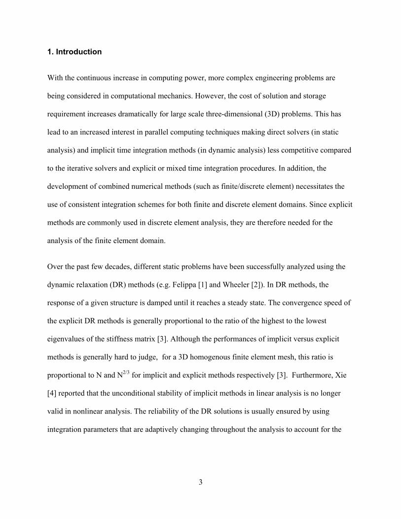
1. Introduction

With the continuous increase in computing power, more complex engineering problems are

being considered in computational mechanics. However, the cost of solution and storage

requirement increases dramatically for large scale three-dimensional (3D) problems. This has

lead to an increased interest in parallel computing techniques making direct solvers (in static

analysis) and implicit time integration methods (in dynamic analysis) less competitive compared

to the iterative solvers and explicit or mixed time integration procedures. In addition, the

development of combined numerical methods (such as finite/discrete element) necessitates the

use of consistent integration schemes for both finite and discrete element domains. Since explicit

methods are commonly used in discrete element analysis, they are therefore needed for the

analysis of the finite element domain.

Over the past few decades, different static problems have been successfully analyzed using the

dynamic relaxation (DR) methods (e.g. Felippa [1] and Wheeler [2]). In DR methods, the

response of a given structure is damped until it reaches a steady state. The convergence speed of

the explicit DR methods is generally proportional to the ratio of the highest to the lowest

eigenvalues of the stiffness matrix [3]. Although the performances of implicit versus explicit

methods is generally hard to judge, for a 3D homogenous finite element mesh, this ratio is

proportional to N and N2/3 for implicit and explicit methods respectively [3]. Furthermore, Xie

[4] reported that the unconditional stability of implicit methods in linear analysis is no longer

valid in nonlinear analysis. The reliability of the DR solutions is usually ensured by using

integration parameters that are adaptively changing throughout the analysis to account for the

4

nonlinear effects. Although a small time step is required to ensure numerical stability, the

computational cost per time step is generally low.

Oakley and Knight [5] developed an adaptive DR for non-linear hyperelastic structures. An

adaptive time step and mass proportional damping coefficient are calculated based on global

tangent stiffness. Sauvé and Metzger [6] applied the DR to solve geometrically nonlinear

structural engineering problems with creep material. A modification to the mass proportional

damping is developed by Metzger [7] to avoid the deleterious effects of sudden changes in the

damping coefficient. Shoukry et al. [8] used the DR with constant time step to study the response

of the pavement under thermal loading.

Given the numerical efficiency of the DR methods, attempts have been made to solve

geotechnical engineering problems involving highly nonlinear material models. Siddiquee et al.

[9] proposed an explicit dynamic relaxation technique to simulate the bearing capacity of a strip

footing on sand under plane strain condition. The time step was kept constant and several

techniques were proposed to maintain the stability of the integration (e.g. load control, arc length

control and displacement control). However, the above technique requires a careful user control

to maintain the stability of the analysis. Tanaka [10] applied the same techniques to study the

response of a single element under plane strain condition. The simulations were carried out

assuming plane strain and using a fine mesh of linear quadrilateral element.

As the stress state violates the failure criteria, the element stiffness can no longer be calculated

purely based on elastic formulation. The stiffness of the element often decreases significantly

when plasticity occurs. Since the time step depends on the element stiffness, the time step can be

adjusted as plasticity develops resulting in accelerated steady state.

5

In this study, a modified framework of dynamic relaxation applicable to plastic material is

proposed. The time step is calculated based on the element consistent tangent stiffness that

depends on the constitutive model. The algorithm is validated by simulating the bearing capacity

of a strip and square footings. The effect of the adaptive time step calculated based on element

consistent tangent stiffness is also evaluated. In addition, the performance of several solid

elements commonly used in 3D analysis is examined.

The developed algorithm and the finite element library were implemented as a finite element

package into the Discrete Element Open Source code YADE [11] using C++ programming as

part of the ongoing development of a generalized discrete-finite element framework for

geotechnical applications.

2. Governing Equations and Force Description

The developed algorithm was based on the adaptive dynamic relaxation (ADR) method proposed

by Oakley and Knight [5] with the addition of a simple plasticity model. The spatial

discretization of a damped structural system can be written as

PxMxCKx =++ &&& (1)

where K, C and M are the stiffness, damping and the mass matrix, respectively; x represents the

displacement vector and P is the external force vector. The internal force vector F can be

assembled on an element by element basis.

The solution of Eq. (1) was obtained using an explicit time integration technique. In this study

the central-difference scheme was adopted as it has been proven to be computationally efficient

[4]. To avoid the need for the assembly and factorization of the global matrices, a mass

6

proportional damping (cM) together with a diagonal mass matrix (M) obtained using mass

lumping were employed. The lumped mass matrix can also increase the numerical stability of the

explicit time integrator [12]. The errors introduced by the lumped masses are compensated for by

the central difference operator [13]. Eq. (1) can therefore be written as

PxMxcMKx =++ &&& (2)

where c is the damping coefficient for mass proportional damping.

3. Time Step Equation

In the central difference method, the velocities are defined at the mid point of the time step, and

the approximation for the temporal derivatives is given as:

)(1 12/1 nnn xxt

x −Δ

= ++& (3)

)(1 1 nnn xxt

x &&&& −Δ

= + (4)

where tΔ is the fixed time step increment. There are generally two options to derive an

incremental relationship: 1) assuming constant acceleration over tΔ ; 2) assuming constant

velocity over tΔ . In this study, the latter assumption was adopted and the velocity was taken as

the average value over tΔ :

)(21 2/12/1 −+ += nnn xxx &&& (5)

Substituting Eq. (3), (4) and (5) into Eq. (2), the expressions for advancing the velocity and

displacement vectors, respectively, can be written as:

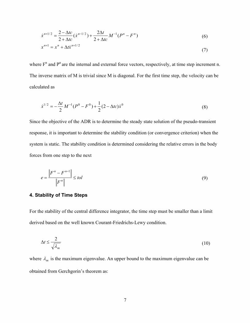
7

)(2

2)(22 12/12/1 nnnn FPM

tctx

tctcx −

Δ+Δ

+Δ+Δ−

= −−+ && (6)

2/11 ++ Δ+= nnn xtxx & (7)

where Fn and Pn are the internal and external force vectors, respectively, at time step increment n.

The inverse matrix of M is trivial since M is diagonal. For the first time step, the velocity can be

calculated as

00012/1 )2(21)(

2xtcFPMtx && Δ−+−

Δ−= − (8)

Since the objective of the ADR is to determine the steady state solution of the pseudo-transient

response, it is important to determine the stability condition (or convergence criterion) when the

system is static. The stability condition is determined considering the relative errors in the body

forces from one step to the next

tolF

FFe

n

nn

≤−

=−1

(9)

4. Stability of Time Steps

For the stability of the central difference integrator, the time step must be smaller than a limit

derived based on the well known Courant-Friedrichs-Lewy condition.

m

tλ2

≤Δ (10)

where mλ is the maximum eigenvalue. An upper bound to the maximum eigenvalue can be

obtained from Gerchgorin’s theorem as:

8

∑=

≤n

j ii

ijm M

K

1maxλ (11)

where Kij is an element of the element consistent tangent stiffness matrix. Kij is derived from the

return mapping algorithm described in the constitutive modeling section. It should be noted that

both the mass (either real or virtual) and time step size are not independent. Adjusting the mass

can lead to inaccurate results particularly when time dependent loading is applied. Thus the mass

has been fixed in the proposed algorithm and the time step has been adjusted based on the

changes in the element consistent tangent stiffness.

5. Optimal Convergence

Rapid convergence is usually obtained when the ratio of the maximum to minimum eigenvalues

is as small as possible. As shown by Oakley and Knight [5], the optimal convergence condition

is reached if

02 λ≤c (12)

where 0λ is the minimum eigenvalues. To estimate the minimum eigenvalue, the mass-stiffness

Rayleigh quotient can be used such that

2/12/1

2/12/1

0 )()(

−−

−−

≅ nTn

nnTn

xMxxSx&&

&&λ (13)

where S is the lumped stiffness matrix for linear problems. For nonlinear problem, Sn is

determined as follows

2/1

1

−

−

Δ−

≅ n

nnn

xtFFS

& (14)

9

No additional parameters are required as the algorithm automatically adjusts the optimal

damping coefficient and the time step based on the changes in the element consistent tangent

stiffness.

6. Constitutive Model

Plasticity models in geomechanics can be integrated using either explicit integration (forward

Euler) or implicit integration (backward Euler). The first is simple to be implemented and

generally is employed for element-base analysis. However, if the material is highly nonlinear,

much iteration may be needed to return the stress state to the failure surface. Moreover, as the

stress state violates the failure criteria, the element stiffness can no longer be calculated purely

by elastic formulation. Since the element stiffness decreases significantly when plasticity

develops and the time step depends on the element stiffness (see Eq. (10)), the time step can

therefore be increased resulting in that the steady state condition can be achieved faster. The

closest point projection method (CPPM) with consistent elastoplastic modulus was utilized at the

Gauss points to calculate the element tangent stiffness. The procedure to derive the consistent

tangent stiffness is described below.

In CPPM, the increments of plastic strain are calculated at the end of each iteration step.

Similarly, the yield condition is enforced at the end of the step (Simo and Hughes [14]). The

integration scheme is written in incremental form as

dqqdd p λλε Δ+Δ= )( (15)

)( pe ddDd εεσ −= (16)

10

0== σdadf T (17)

where pdε , σd and εd is the incremental plastic strain, incremental stress and incremental total

strain respectively; λΔ is the plastic multiplier.

⎟⎠⎞

⎜⎝⎛∂∂

=σfa (18)

where f is the yield function.

σσ

dqdq ⎟⎠⎞

⎜⎝⎛∂∂

= (19)

where q is the derivative of the plastic flow potential function g with respect to stress.

Plastic multiplier can be updated consequently at iteration (k+1)th based on iteration kth

kkk δλλλ +Δ=Δ +1 (20)

where kδλ is the increment in λΔ at k iteration. kδλ is calculated as follows

)()()(

)()()(

kkTk

kkTkkk

qRarRaf −

=δλ (21)

where

ekekk DqDIR1

)(−

⎥⎦⎤

⎢⎣⎡

∂∂

Δ+=σ

λ (22)

and

qr pdaccumulate

pk λεε Δ++−= (23)

11

where pdaccumulateε is the total plastic strain accumulated at the previous load step.

Substituting Eq. (15) into (16) with condition given by Eq. (17) and solving for d( λΔ ) gives

RdqaRdad T

T ελ =Δ )( (24)

Substituting into Eq. (16) gives

εσ dDd c= (25)

where Dc is the consistent elastoplastic modulus calculated as

Rqa

RRqaRD T

TC −= (26)

To approximate the consistent stiffness of the element, the B matrix derived from the shape

function of the element was employed. The element consistent tangent stiffness ceK then can be

determined as:

∫Ω

Ω=e

BdDBK CTce (27)

The flow chart used in the development of the proposed algorithm is shown in Fig. 1.

7. Calibration of the Proposed Algorithm

The proposed algorithm was used to simulate the bearing capacity of a strip and square footings

in weightless soil. The footings were assumed to be rigid enough to create uniform pressure on

the supporting soil. The Mohr Coulomb (MC) failure criterion with non associated flow rule was

utilized in both cases. Local rounding at the corners of the MC failure surface in the principal

12

stress space was used as described by Smith and Griffiths [15]. The material properties are

summarized in Table 1. The calculated load displacement behaviour for the two investigated

cases was established and compared with the conventional static analysis using the same mesh

and material properties.

Theoretically, the bearing capacity can be calculated as

cult cNq = (28)

where Nc is the bearing capacity factor expressed as (Prandtl, [16])

φcot)1( −= qc NN (29)

where

φπφ tan2 )2/45(tan eNq += (30)

For the drained case Nc = 14.83 and qult = 520 kPa; for the undrained case Nc = 5.14 and qult =

514 kPa

Strip footing

The analyzed footing is 4 m wide and supported by Mohr Coulomb drained material. Drained

condition was carried out using plane strain analysis. Considering the symmetry of the problem,

only one half of the footing was analyzed. Quadratic quadrilateral elements with reduced

integration (4 Gauss points) were employed in the simulation. The problem geometry and the

finite element mesh are shown in Fig. 2. In order to capture the failure load, a uniform pressure

of 200 kPa was first applied at the initial step. After the stability condition (expressed by Eq. (9))

was reached, the load was then increased to the next step. A tolerance value of 1e-6 was adapted

13

in the present analysis. Seven load increments of: 200 kPa, 300 kPa, 350 kPa, 400 kPa, 450 kPa,

480 kPa and 500 kPa were applied to approach the expected failure load. The load was

subsequently increased (1 kPa increments) up to failure which is characterized by the numerical

instability of the system.

In conventional implicit analysis, the applied load must be divided into several increments to

reach convergence and maintain stability. If the stress state is far from the yield surface, the

correct stress state cannot be easily determined. To demonstrate the robustness of the algorithm

in modelling highly nonlinear material, the total load was applied in one single step and the

displacement results were compared with the previous multi-step analysis.

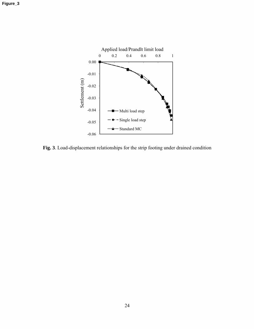
As shown in Fig. 3, the results of the dynamic relaxation analyses are in good agreement with

those obtained using the conventional static analysis. Both of the simulations captured the

theoretical Prandtl failure load (514 kPa). It can also be seen that the single step loading has

successfully produced the same response.

Square footing

The bearing capacity of a square footing 4 m x 4 m was analyzed under both drained and

undrained conditions. A schematic of the problem geometry and the 3D finite element mesh

(1728 elements) are illustrated in Fig. 4. Due to the symmetry, only 1/4 of the footing was

modeled. The mesh in the vicinity of the footing was refined to capture the rapid changes in

displacement gradients. Smooth rigid side boundaries and a rough rigid base boundary were used

in the analysis.

14

The performance of four different finite elements was also investigated in terms of speed and

accuracy. The examined element types are listed below:

1. Reduced integration twenty-node quadratic brick elements (20N8I)

2. Mixed integration rule eight-node quadratic brick elements (8NS8I) (Simo and Rifai,

[17])

3. Reduced integration eight-node quadratic brick elements (8N1I)

4. Reduced integration eight-node quadratic brick elements with stiffness hourglass control

(8NH1I) (Belytschko and Ong [18])

The finite element meshes generated using the above elements were further refined to examine

the effect of the element size on the calculated displacements. As shown in Fig. 5, the load

displacement curves exhibited little difference in all of the examined cases. The failure loads

captured by the different elements varied from 1.08 to 1.23 times of the Prandlt load. The

calculated values are consistent with those reported by Salgado et al. [19] for rectangular

footings. It is worth noting that the captured failure loads and the load displacement behaviour of

the 8NH1I elements varied depending on the value of the anti hourglass parameter.

It was also found that the 8N1I element (usually unstable element due to the deficient stiffness

ranking) performed reasonably well using the proposed algorithm. Similarly for the undrained

analysis where soil experienced constant volume deformation, no hourglass displacements were

observed. This can be explained by the dominating shear failure of the supporting soils. The

computational times for all examined cases are summarized in Table 2. It can be seen that the

20N8I required the most time among all examined elements, however, it provided an accurate

15

failure load prediction. 8NH1I and 8N1I elements are the most economical in terms of analysis

time meanwhile the accuracy is preserved. However, due to the formulation deficiency, the use

of 8N8Iis not recommended for collapse analysis. It is concluded that the 8NH1I has maintained

the balance between the calculation speed and the accuracy and therefore is considered to be the

best choice for the above type of analysis.

8. Effect of Using Adaptive Time Step Scheme

The effect of the adaptive time step in 2D and 3D analyses is illustrated in Fig. 6. When the load

applied was less than 45% of the failure load, no significant effect was observed. However,

increasing the applied load to about 70% of the failure load resulted in an increase in the number

of iterations needed for convergence in both the constant time step and adaptive time step

schemes. However, the constant time step scheme required 1.4 times the number of iterations

needed for the adaptive time step scheme. The ratio slightly decreased as the applied load

approached failure and the difference between the two schemes decreased to about 1.2.

9. Numerical Example

A square footing supported by Mohr Coulomb drained material is analyzed using the developed

algorithm adopting the problem geometry shown in Fig. 4. The soil unit weight is assumed to be

18 kN/m3 with friction angle of 30o. The material properties used in the analysis are provided in

Table 1. The bearing capacity of the footing has also been calculated based on Terzaghi [20]

bearing capacity theory:

γγBNqNcNq qcult 21

++= (31)

16

where q is the overburden pressure; γ is the soil unit weight; B is the footing width; Nγ is

derived by Michalowski [21] as follows:

φφγ tantan11.566.0 += eN (32)

Thus for sand with friction angle of 30, a value of 771 kN/m2 is obtained for the bearing capacity

of the square footing.

The same mesh in the previous section was used with 8NH1I elements (see Fig. 4). An additional

feature of the analysis is the activation of the soil unit weight and the initial stresses assigned at

Gaussian stress points. The coordinates of each Gauss point are calculated using the

isoparametric property of the element

∑=

=8

1iii yNy (33)

where N is the shape function of the brick element and y is the vertical coordinate of the element

nodes. Only the y coordinate is required in this case and the vertical stress yσ is obtained after

multiplication by the soil unit weight (Table 1). The normal effective stresses xσ and zσ are

obtained by multiplying yσ by the earth pressure coefficient at rest (K0) calculated using [Jaky,

22]:

φsin10 −=K (34)

The analysis consists of two stages: Geostatic stage and failure load analysis. In the geostatic

stage, the soil weight is activated and the equilibrium is first obtained. In the next stage, the same

procedure used in section 7 is employed to determine the failure load.

17

As shown in Fig. 7, the calculated failure load is found to be 862 kN/m3, the ratio of the

calculated value to the theoretical value (approximately 1.12) agrees well with that reported by

Ming and Michalowski [23]. It is worth noting the analysis reported by Ming and Michalowski

[23] employing the implicit methods required the use of a cohesion value of 3.6 kPa in order to

maintain convergence whereas in the present study no such assumption was needed to achieve

convergence.

10. Summary and Conclusions

An adaptive dynamic relaxation method applicable to geotechnical applications was developed

and implemented in this study. The use of diagonal mass and damping matrices with central

difference time integrator has proven to be an effective numerical approach for problems

involving material nonlinearity. Adjusting the adaptive time step based on the changes in the

element consistent tangent stiffness resulted in a decrease in the number of iterations needed for

convergence by up to 40% compared to the constant time step schemes. In the proposed

algorithm, the time step and damping values were automatically adjusted to achieve an optimal

convergence while maintaining the stability of the system. The robustness and accuracy of the

algorithm were demonstrated by analyzing the bearing capacity of strip and square footings.

The performance of four different brick elements was also evaluated. The accuracy of the eight-

node brick element with stiffness hourglass control was found to be heavily dependent on the

user experience. Finally, since the proposed finite element algorithm employs a explicit dynamic

scheme that is commonly adopted in Discrete Element analysis, it in can be easily combined with

a Discrete Element code in developing a hybrid Discrete-Finite element suitable for geotechnical

engineering applications.

18

Acknowledgement

This research is supported by a research grant from the Natural Sciences and Engineering

Research Council of Canada (NSERC). The financial support provided by McGill Engineering

Doctoral Award (MEDA) to the first author is greatly appreciated.

References

[1] Felippa, CA. Dynamic relaxation in quasi-Newton methods. In C. Taylor, E. Hinton, DRJ Owen and D. Onate (eds.), Numerical Methods for Nonlinear Problems. Swansea, 1986; 27-38.

[2] Underwood, PG. Dynamic Relaxation: A review. In T. Belytschko and TJR. Hughes (eds.), Computational Methods for Transient Dynamic Analysis, Chapter 5, North Holland, Amsterdam. 1983.

[3] Munjiza, A. The combined finite-discrete element method, John Wiley & Sons Ltd, England. 2004.

[4] Xie, YM. An assessment of time integration schemes for non-linear dynamic equations. Journal of Sound and Vibration, 1996; 192(1): 321-331.

[5] Oakley, DR, Knight, NF. Adaptive dynamic relaxation algorithm for non-linear hyperelastic structures Part I. Formulation. Computer Methods in Applied Mechanics and Engineering, 1995; 126(1): 67-89.

[6] Sauvé, RG, Metzger, DR. Advances in Dynamic Relaxation Techniques for Nonlinear Finite Element Analysis, Journal of Pressure Vessel Technology, 1995; 117, 170-176.

[7] Metzger DR. Adaptive damping for dynamic relaxation problems with non-monotonic spectral response. International Journal for Numerical Methods in Engineering, 2003; 56: 57–80

[8] Shoukry, SN, William, GW, Riad, MY, McBride, K.C. Dynamic Relaxation: A Technique for Detailed Thermo-Elastic Structural Analysis of Transportation Structures. International Journal for Computational Methods in Engineering Science and Mechanics, 2006; 7(4): 303-311.

[9] Siddiquee, MSA, Tanaka, T, Tatsuoka, F. Tracing the equilibrium path by dynamic relaxation in materially nonlinear problems. International Journal for Numerical and Analytical Methods in Geomechanics, 1995; 19(11): 749-767.

[10] Tanaka, T. Viscoplasticity of geomaterials and finite element analysis. In Soil Stress Strain Behavior: Measurement, Modeling and Analysis, Geotechnical Symposium in Rome, March, 2006; 769-778.

[11] Kozicki, J. Donze, FV. Applying an open-source software for numerical simulations using finite element or discrete modelling methods. Computer Methods in Applied Mechanics and Engineering, 2008; 197(49-50): 4429-4443.

[12] Belytschko, T. Mullen, R. Explicit integration of structural problems. In: Finite Elements in Nonlinear Mechanics, TAPIR, Trondheim, 1978.

19

[13] Krieg, R, Key, S. Transient shell response by numerical time integration. International Journal of Numerical Methods in Engineering, 1973; 17: 273–286.

[14] Simo, JC, Hughes, TJR. Computational inelasticity, Springer, New York, 1998. [15] Smith, IM, Griffiths, DV. Progamming the finite-element method, 4th Ed., Wiley, New

York, 2004. [16] Prandtl, L. Uber die Eindringungsfestigkeit (Härte) plastischer baustoffe und die

festigkeit von Schneiden. Zeitschrift fur angewandte Mathematik und Mechanik, 1921; 1(1): 15-20.

[17] Simo, JC, Rifai, MS. A class of mixed assumed strain methods and the method of incompatible modes, International Journal for Numerical Methods in Engineering, 1990; 29, 1595-1638.

[18] Belytschko, T, Ong, S. Hourglass control in linear and nonlinear problems, Computer Methods in Applied Mechanics and Engineering, 1984; 43, 251-276.

[19] Salgado, R, Lyamin, A, Sloan, S, Yu, HS. Two- and Three-dimensional Bearing Capacity of Footings in Clay. Geotechnique, 2004; 54(5): 297-306.

[20] Terzaghi, K. Theoretical soil mechanics, Wiley, New York. 1943 [21] Michalowski, R. L. An estimate of the influence of soil weight on bearing capacity using

limit analysis. Soils Found, 1997; 37(4): 57–64. [22] Jaky J. Pressure in soils, 2nd ICSMFE, London, 1: 103-107. [23] Ming, Z., and Michalowski, R. L., Shape Factors for Limit Loads on Square and

Rectangular Footings, Journal of Geotechnical and Geoenvironmental Engineering, 131: 223-231.

20

Table 1 Material properties

Cases Cohesion (Pa)

Friction angle

(degree)

Dilation angle

(degree)

Poisson’s ratio

Young’s modulus

(Pa)

Unit weight

(kN/m3)Strip footing drained condition 35 20 0 0.3 1 x 105 0

Square footing drained condition 35 20 0 0.3 1 x 105 0

Square footing undrained condition 100 0 0 0.49 1 x 105 0

Square footing drained condition (used in the numerical example)

0.1 30 30 0.3 1 x 106 18

21

Table 2 Computation time (minutes) Cases 20N8I 8NS8I 8NH1I 8N1I Square footing drained condition 156 12 4 3

Square footing undrained condition 195 30 6 5

22

Fig. 1. Flow chart for the adaptive explicit dynamic relaxation

Figure_1

23

Fig. 2. Finite element mesh used in the strip footing analysis

2 m

12 m

6 m

Figure_2

24

-0.06

-0.05

-0.04

-0.03

-0.02

-0.01

0.000 0.2 0.4 0.6 0.8 1

Settl

emen

t (m

)

Applied load/Prandlt limit load

Multi load step

Single load step

Standard MC

Fig. 3. Load-displacement relationships for the strip footing under drained condition

Figure_3

25

Fig. 4. Geometry and finite element mesh for the square footing

12m

12 m

2 m

12 m

2 m Square footing location

Figure_4

26

-0.07

-0.06

-0.05

-0.04

-0.03

-0.02

-0.01

0.000 0.4 0.8 1.2

Settl

emen

t (m

)

Applied load/Prandlt limit load

8NH1I

8N1I

8NS8I

20N8I

Standard MC

-0.07

-0.06

-0.05

-0.04

-0.03

-0.02

-0.01

0.000 0.4 0.8 1.2

Settl

emen

t (m

)

Applied load/Prandlt limit load

8NH1I

8N1I

8NS8I

20N8I

Standard MC

Fig. 5. Load-displacement relationships for the square footing:

a) drained condition; b) undrained condition

a)

b)

Figure_5

27

1.00

1.10

1.20

1.30

1.40

1.50

0.40 0.60 0.80 1.00

Nor

mal

ized

num

ber o

f ite

ratio

ns

(Nco

nsta

nt /

Nad

ativ

e)

Applied load/Failure load

2D

3D

Fig. 6. Comparison between constant and adaptive time step schemes

Figure_6

28

-0.35

-0.30

-0.25

-0.20

-0.15

-0.10

-0.05

0.000 0.2 0.4 0.6 0.8 1 1.2

Settl

emen

t (m

)

Normalized applied vs. theoretical load

Fig. 7. Load-displacement relationships for a square footing on sand

Figure_7