Es

Ea

b

c

d

a

ARA

KMTLG

1

vp(11bamsIs

n

0h

International Journal of Applied Earth Observation and Geoinformation 26 (2014) 286–297

Contents lists available at ScienceDirect

International Journal of Applied Earth Observation andGeoinformation

jo ur nal home p age: www.elsev ier .com/ locate / jag

valuating suitability of MODIS-Terra images for reproducing historicediment concentrations in water bodies: Lake Tana, Ethiopia

ssayas Kabaa,c,d,∗, William Philpotb, Tammo Steenhuisa,c

Department of Biological and Environmental Engineering, Cornell University, Ithaca, NY, USADepartment of Civil and Environmental Engineering, Cornell University, Ithaca, NY, USASchool of Civil and Water Resources Engineering, Bahir Dar University, Bahir Dar, EthiopiaGeospatial Data and Technology Center, Bahir Dar University, Bahir Dar, Ethiopia

r t i c l e i n f o

rticle history:eceived 13 December 2012ccepted 9 August 2013

eywords:ODIS

SSake Tanaetis–Ord Gi*

a b s t r a c t

Government and NGO funded conservation programs are being implemented in developing countrieswith the potential benefit of reduced sediment inflow into fresh water lakes. However, these claimsare difficult to verify due to limited historical sediment concentration data in lakes and rivers. Remotesensing can potentially aid in monitoring sediment concentration. With almost daily availability overthe past ten years and consistent atmospheric correction applied to the images, Moderate ResolutionImaging Spectroradiometer (MODIS) 250 meter images are potential resources capable of monitoringfuture concentrations and reconstructing historical sediment concentration records. In this paper, site-specific relationships are developed between reflectance in near-infrared (NIR) images and three factors:total suspended solids (TSS), turbidity and Secchi depth for Lake Tana near the mouth of the GumaraRiver. The first two sampling campaigns on November 27, 2010 and May 13, 2011 are used in calibration.Reflectance in the NIR varies linearly with turbidity (R2 = 0.89) and TSS (R2 = 0.95). Secchi depth fit best toan exponential relation with R2 of 0.74. The relationships are validated using a third sample set collectedon November 7, 2011 with RMSE of 11 Nephelometric Turbidity Units (NTU) for Turbidity, 16.5 mg l−1

for TSS and 0.12 meters for Secchi depth. The MAE was 10% for TSS, 14% for turbidity and 0.1% for Secchidepth. Using the relationship for TSS, a 10-year time series of sediment concentration in Lake Tana near theGumara River was plotted. It was found that after the severe drought of 2002 and 2003 the concentrationin the lake increased significantly. The results showed that MODIS images are potential cost effective toolsto monitor suspended sediment concentration and obtain a past history of concentration for evaluating

ment

the effect of best manage

. Introduction

Reduced sediment inflow decreases sedimentation of reser-oirs, ensures sunlight penetration in lake water, improves theroductivity of the whole food web in the aquatic systemVijverberg et al., 2009), increases zooplankton growth (Lind et al.,992) and makes water supply disinfection more effective (Gadgil,998). In the Ethiopian highlands, conservation practices areeing installed by government and NGO’s to reduce soil erosionnd thereby reduce sediment concentration in streams. Despiteillions of dollars invested (Betru and Sonali, 2010), very few mea-

urements are available on the effectiveness of these interventions.n few cases, soil and water conservation practices have decreasedediment concentrations (Herweg and Ludi, 1999; Nyssen et al.,

∗ Corresponding author at: Department of Biological and Environmental Engi-eering, Cornell University, Ithaca, NY, USA.

E-mail addresses: ekk45@cornell.edu, essayask@gmail.com (E. Kaba).

303-2434/$ – see front matter © 2013 Elsevier B.V. All rights reserved.ttp://dx.doi.org/10.1016/j.jag.2013.08.001

practices.© 2013 Elsevier B.V. All rights reserved.

2008). However, in general there is not a downward trend insediment concentrations (Tilahun et al., 2013). Some studies sug-gest that 70% of reservoirs built in the last 20 years have serioussiltation problems and that the useful life will end well before thedam design period (Haregeweyn et al., 2006). With the constructionof new hydroelectric dams in Ethiopia it becomes more and moreimportant to assess the effectiveness of conservation practices. Oneof the ways that this can be accomplished is by measuring sedi-ment concentration and turbidity in water bodies (Delmas et al.,2011; Villar et al., 2012). Turbidity gradients also help in identify-ing and interpreting geomorphologic and hydrological processes,as sediment transport, deposition and re-suspension (Güttler et al.,2013).

Intensive sampling of either sediment concentration (gravi-metric) or turbidity (by optical Secchi disk) on many locations is

prohibitively expensive and has led to efforts to map these param-eters using remotely sensed images (Chen et al., 2007; Nechad et al.,2010; Wang and Lu, 2010a; Hashimoto and Oki, 2012). Table 1 givessome of these relationships of remotely sensed reflectance and

E. Kaba et al. / International Journal of Applied Earth Observation and Geoinformation 26 (2014) 286–297 287

Table 1Correlations between different MODIS band reflectance and water quality parameters suggest site specific regression equations.

Parameter Equationa r2

Turbidity (NTU) 1203.9 × R1.087b1

0.73 Chen et al. (2007)

SSC (mg l−1) −23.03 + 60.24 × (Rb1 − Rb5) 0.73 Wang and Lu (2010a)

Log(TSS) (mg l−1) 0.1497e{1.859[log(Rb2)

10/log(Rb1)

10]} 0.61 Wang and Lu (2010a)

1.5144[log(Rb2)10 /log(Rb1)

10 ] − 0.5755 0.72

SS (mg l−1) 0.24e188.3×Rb1 0.90 Min et al. (2012)

xamp

seci(drttosT

1

tarahttWews2tacacmatiss

bcaip

2

wc

The MODIS-Terra satellite has been acquiring images of theentire globe since 2000 in 36 spectral bands with 250-m,

SSC (mg l−1) 0.95e(2.15×Rb4/Rb1)

a R refers to reflectance and b followed by a number refers to band number, for e

ediment concentration which are site specific (Liu et al., 2003; Maot al., 2012) due to two factors: first the combination of subjectiveriteria used by researchers in atmospheric correction, with empir-cal calibration factors for correcting the sensitivity of the sensorFroidefond et al., 1999) and second, the infinite combinations ofiverse water constituents create a wide variation in the spectraleflectance of shallow waters (Baban, 1993; Chami et al., 2006). Inhis paper a site specific relationships is developed for mapping TSS,urbidity and Secchi depth on Lake Tana. The relationship devel-ped for TSS is used to construct a ten year sequence of suspendedediment concentrations for the Gumara River that flows to Lakeana.

.1. Remote sensing platform

The use of remotely sensed images for sediment concentra-ion estimation has to strike a balance between ease of accessnd processing, sensitivity to change in water color, and tempo-al resolution of the remotely sensed data. In addition, the rigoroustmospheric correction required in using remotely sensed imagesas been a major source of uncertainty in the past because ofhe extreme sensitivity of most atmospheric correction algorithmso subtle changes in the visible spectrum (Jolivet et al., 2007;

erdell et al., 2010). Recent developments in remote sensing havenabled the global science community to have access to imagesith consistent atmospheric correction applied to them. One

uch achievement is the MODIS-Terra version-5 validated Stage products (USGS, 2011). MODIS has detectors in spectral regionshat provide direct measurements of atmospheric scattering andbsorption (Kaufman et al., 1998; Li et al., 2003) leading to a moreonsistent atmospheric correction. The release of these productsvoids the effort required for sensor calibration and atmosphericorrection. The accuracy of these products has been confirmed atany locations and time periods (USGS, 2011). MODIS images are

vailable on a daily basis making it possible to analyze TSS andurbidity dynamics (Min et al., 2012). MODIS medium-resolutionmages (250 m) provide the advantage of increased sensitivity foruspended solid observation in that these bands are 4–5 times moreensitive than the L7-ETM+ bands (Hu et al., 2004).

Correlations between MODIS measured reflectance and tur-idity, total suspended matter (TSM), suspended sedimentoncentration (SSC) and/or TSS have been reported by severaluthors. The equations and correlations from the most recent stud-es using MODIS images to quantify water quality parameters areresented in Table 1.

. Materials and methods

Lake Tana (Fig. 1) is situated on the basaltic plateau of the north-estern highland of Ethiopia (12◦N, 37◦15′E, and 1800 m altitude)

overing an area of over 3000 km2.

0.88 Bi et al. (2011)

le Rb1 refers to reflectance from band one.

The lake drains a catchment area of 16,000 km2. Six permanentrivers and 40 small seasonal rivers feed the lake. The shallow lake(average depth 9 m) is Ethiopia’s largest lake, containing half thecountry’s freshwater resources, and is the third largest in the NileBasin (Vijverberg et al., 2009). The most pronounced advantage ofLake Tana is its storage characteristics, in that it accommodates alive storage which amounts to more than two times that of the fivelarge reservoirs in Ethiopia,1 rendering a relatively low cost perunit of utilizable water (Gebeyehu, 2004). A bathymetric surveyundertaken in 2006 showed that the lake has a maximum depthof 15 m and stretches 65 km west-east and 74 km south-north(Ayana, 2007). The main rainy monsoon season begins in June andlasts through September and temperature varies between day timeextremes of 30 ◦C to night lows of 6 ◦C. The minimum recordedannual precipitation was 966 mm in the year 2002 and the annualmaximum was 1998 mm in the year 1997 (Yilma and Awulachew,2009).

2.1. TSS, turbidity and Secchi depth measurements

Three campaigns were carried out to collect water samples andmeasure Secchi depth during the satellite overpass time over LakeTana near the mouth of the Gumara River with a mean flow of60 m3/s during the rainy season. Separate campaigns were con-ducted during the mornings of November 27, 2010, May 13, 2011and November 7, 2011. Samples were collected along transectsparallel to the shore during each overpass (Fig. 2). Ground mea-surements were done within ±15 min of the seconds-long satelliteoverpass (i.e. a 30 min period centered on 10:30 AM). Concurrentmeasurements are crucial as sediment concentrations during highstream flow or wind can change quickly (Petus et al., 2010). Ateach location along the sampling path, bulk water samples werecollected from the upper 0.2 m of the water column in a 750 mlcontainer for turbidity and TSS analysis. GPS coordinates of sam-pled locations were also recorded. During sampling the commonlyknown algal bloom areas are excluded to avoid uncertainties in themeasurement.

Total suspended solids measurements were made in laboratoryby drawing 10 ml aliquot from a well mixed container, centrifugingfor ten minutes at 4000 rpm, pouring off supernatant, separatingand drying the retained solids, and weighing. Turbidity measure-ments were made using a Hach 2100N turbidimeter calibratedusing formazin solution.

2.2. MODIS data

1 Gilgel Gibe, Koka, Finchaa, Amerti, and Melka Wakena, provide an aggregatestorage capacity of about 4.4 billion m3, compared to Lake Tana’s live storage of 9billion m3.

288 E. Kaba et al. / International Journal of Applied Earth Observation and Geoinformation 26 (2014) 286–297

Fig. 1. In this 13 June 2000 MODIS image a turbid plume flows into the lake turning the shore and stream mouth locations to reddish brown and raising the water reflectance.(For interpretation of the references to color in this figure legend, the reader is referred to the web version of the article.)

Table 2Numbers of lake samples for the campaign days.

Parameter Unit Calibration Validation

November 27, 2010 # of samples May 13, 2011 # of samples November 7, 2011 # of samples

5aoanireefiit2us

2d

ra

tions of red and near infrared red (NIR) bands (Table 3). Followingthe work of Wang et al. (2010), several combinations of bands wereused (e.g. sum, the difference and ratio of reflectance of the twobands) to increase the goodness of fit of the regression equations.

Table 3Estimation statistics for various band combinations; bold numbers have the largestR2.

Band combination R2 Adjusted R2 Standard error Significance F

Turbidity (n = 43, mean = 100.03 NTU)NIR 0.89 16.57 0.000NIR/Red 0.76 0.75 25.26 0.000NIR + Red 0.08 0.06 49.4 0.063Red − NIR 0.48 0.47 37.04 0.000(Red − NIR)/(Red + NIR) 0.69 0.68 28.6 0.000

TSS (n = 54, mean = 48.43 mg l−1)NIR 0.95 10.77 0.000NIR/Red 0.89 0.88 16.86 0.000NIR + Red 0.76 0.76 24.34 0.000Red − NIR 0.86 0.85 18.96 0.000

Turbidity NTU 30

TSS mg l−1 30

Secchi depth m 30

00-m, and 1000-m spatial resolutions. The red (620–670 nm)nd NIR (841–876 nm) bands labeled ‘MOD09GQ’ are availablen a nearly daily basis at 250 m spatial resolution. These imagesre sensitive for turbid water applications (Hu et al., 2004). Aumber of previous studies have successfully used MODIS 250 m

mages to establish a reflectance–TSS, reflectance–turbidity andeflectance–Secchi depth relationships (Chen et al., 2007; Petust al., 2010; Miller and McKee, 2004; Dall’Olmo et al., 2005; Kutsert al., 2006). In this study MODIS Terra data are used because oureld samples were taken in the morning corresponding to Terra’s

maging time. MODIS red and NIR 250 m images corresponding tohe field water sampling dates (i.e. 27 November 2010, 13 May011 and 7 November 2011) were downloaded from the USGS sitesing MODIS Reprojection Tool Web Interface (MRTWeb).2 Table 2ummarizes the observations for the respective dates.

.3. MODIS reflectance relationship to TSS, turbidity and Secchiepth

In order to obtain the relationship between the MODISeflectance and indicators of sediment concentration in the lake

multiple regression analysis was performed on various combina-

2 https://mrtweb.cr.usgs.gov/.

51 3051 3451 30

(Red − NIR)/(Red + NIR) 0.88 0.88 16.92 0.000

Secchi depth (n = 73, mean = 0.22 m)NIR 0.74 0.02 0.000NIR/Red 0.58 0.57 0.03 0.000NIR + Red 0.50 0.49 0.03 0.000Red − NIR 0.38 0.36 0.03 0.000(Red − NIR)/(Red + NIR) 0.57 0.56 0.03 0.000

E. Kaba et al. / International Journal of Applied Earth Observation and Geoinformation 26 (2014) 286–297 289

F in Las

NucelgceiFaa

2c

ret

ig. 2. Three sampling campaigns were conducted near the outlet of Gumara Rivereason on November 27, 2010 and November 7, 2011.

ormalized ratios (NIR to red), band sum and band difference aresed along with single band regression. Samples from the first twoampaigns of November 27, 2010 and May 13, 2011 are used tostablish the relation (i.e. calibration) and the third sample col-ected on November 7, 2011 was used to validate the relation. Theoodness of fit of the models is evaluated based on the resultingoefficient of determination (R2). Adjusted R2 is also calculated forach regression to test if an improvement in the R2 is due to thenclusion of a band to the regression model or a random chance.or the validation step, the accuracies of predicted TSS, turbiditynd Secchi depth were assessed by root mean square error (RMSE)nd mean absolute error (MAE).

.4. Determining historical record of Lake sedimentoncentration near Gumara River

Assuming that the satellite overpass time is the time of theepresentative inflowing concentration of the day, the regressionquations can be applied to archived MODIS images to generateurbidity and TSS time series data for Lake Tana at entry location

ke Tana. During the dry season May 13 2011 and shortly after the end of the rainy

of Gumara River. Due to large cloud cover over the lake duringthe satellite overpass time only few images are available for useduring the rainy season. Thus to avoid large data gaps during therainy season and minimize error a mean monthly reflectance rasterare preferred. The time series data can be used to model turbidityand TSS emissions into Lake Tana. Nevertheless selecting the bestinflow-representative pixel requires careful consideration of actualsituation during sampling and imaging. This pixel represents themaximum TSS at the imaging time. The TSS spreads from this pixelto the neighboring pixels as the result of which the representativepixel is often surrounded by pixels of relatively higher TSS. In thisstudy we used the Getis–Ord Gi* statistic data mining technique toidentify this representative pixel (Ord and Getis, 1995).

The 10-year time span (2000–2009) NIR images of Gumara Riverentering Lake Tana are downloaded from USGS MODIS archive viaMRTWeb. Cloud contaminated images are excluded and the images

are masked with the water sampling location polygon (Hashimotoand Oki, 2012). This location is consistently more turbid in theimages from other times during the rainy season (Fig. 1). A meanmonthly reflectance raster is created using cell statistics operation

290 E. Kaba et al. / International Journal of Applied Earth Observation and Geoinformation 26 (2014) 286–297

Fig. 3. Getis–Ord Gi* analysis extent (December 2000). In a hot spot analysis the Getis–Ord Gi* statistic is calculated for each feature in the analysis extent by looking at eachf the z-score and p-values for each feature with either high or low values cluster spatially.T nded

r

irig

G

wf

t

s

eature within the context of neighboring features. The resulting attribute includeso be a statistically significant hot spot, a feature with a high value must be surrouepresentative value for the monthly TSS.

n ArcGIS. In each mean reflectance image the pixel with the largesteflectance is identified using the Getis–Ord Gi* statistic data min-ng technique (Getis and Ord, 2010). The Getis–Ord Gi* statistic isiven by:

∗i =

∑nj=1wi,jxj − X

∑nj=1wi,j

s

√[∑n

j=1w2

i,j−(∑n

j=1wi,j

)2]

n−1

(1)

here xj is the TSS value for pixel J, wi,j is the spatial weight betweeneature i and j, n is equal to the total number of pixels, X is mean of

he TSS values with in the cut off distance given by X =∑n

j=1xj

n and

=

√∑n

j=1x2

jn − (X)

2

by other features with high values as well. The TSS value of this feature is used as

The Getis–Ord Gi* statistic is used to generate the z score foreach pixel in the NIR raster which will help to identify the high orlow values that are clustered spatially. Each of the pixels withinthe delineated entry location will be looked within the context ofits neighboring pixels. The local sum for a pixel and its neighborsis compared proportionally to the sum of all features; when thelocal sum is much different than the expected local sum, and thatdifference is too large to be the result of random chance, a statisti-cally significant z score results. For statistically significant positivez scores, the larger the z score is, the more intense the clusteringof high values or a hot spot (Mitchell, 2005). A pixel with a high

value and surrounded by other features with high values as well isconsidered a hotspot from where sediment plume spreads out.

A masking polygon is used to extract the pixels at the rivermouth on the lake where the said turbid plumes are visible. The

E. Kaba et al. / International Journal of Applied Earth Observation and Geoinformation 26 (2014) 286–297 291

F cchi dp

mte

ec

ig. 4. Scatter plot of water reflectance (�) against observed Turbidity, TSS and Searameters.

asking polygon encloses 537 (i.e. n in Eq. (1) is 537) pixels inhe mean monthly NIR reflectance image. Fig. 3 shows the analysis

xtent for the Getis–Ord Gi* statistic.

The Getis–Ord Gi* tool in ArcGIS is used in this study to gen-rate the Gi* statistic. In this operation the TSS raster is firstonverted to a point feature in which the value field is the TSS

epth using different band combinations. The NIR band gives the best fit for all the

value picked for each pixel in the analysis extent. Spatial rela-tionship among features is then conceptualized by specifying a

distance up to which the algorithm will seek for similar TSS val-ues. Owing to the actual spatial resolution of the image rasterused (i.e. 231.65 m), a 232 meter distance is used. The analy-sis result is a new output feature class with a z-score (i.e. the

292 E. Kaba et al. / International Journal of Applied Earth Observation and Geoinformation 26 (2014) 286–297

TSS (b

Gc

3

alcdbst

T

w

T

w

S

Fig. 5. November 7, 2011 data is used to validate turbidity (a),

i* statistic) and p-value for each feature in the input featurelass.

. Results

The relationship between MODIS reflectance to TSS, turbiditynd Secchi depth are given in Table 3. In all band combinations ainear relationship was observed between the tested NIR and redombinations of MODIS bands and either TSS, turbidity and Secchiepth (Fig. 4). The relationship between MODIS reflectance to NIRand was superior to other combinations. The calibrated regres-ions between TSS, turbidity, Secchi depth and the reflectance inhe NIR band, �NIR were in order of decreasing r2:

SS = 2371 × �NIR − 62.8 (2)

here TSS is in mg l−1, n = 54, p < 0.001 and r2 = 0.95

urbidity = 3209 × �NIR − 50.1 (3)

here turbidity is in NTU, n = 43, p < 0.001 and r2 = 0.89

ecchi depth = 0.38 × e−12.2X�NIR (4)

) and Secchi depth (c); and associated residuals (d through f).

where Secchi depth is in meters, n = 73, p < 0.001 and r2 = 0.74n, pand r2 respectively are the number of samples used, the probabilitythat such a linear relation is occurring by chance (at 5% significancelevel) is 1 in a 1000, and coefficient of determination of the fit.

Applying these equations to the November 7, 2011 imageresulted in a root mean square error (RMSE) of 16.5 mg l−1, 15.6NTU and 0.11 m in comparison to measured TSS, turbidity and Sec-chi depth respectively. The MAE was 10% for TSS, 14% for turbidityand 0.1% for Secchi depth. The scatter plot for observed and esti-mated turbidity, TSS, and Secchi depth and the residual of theseestimates are shown in Fig. 5. The residuals were distributed within±35 mg l−1 for TSS, ±50 NTU for turbidity, and ±0.05 m for Sec-chi depth. The adjusted R2 is mainly applied when combination ofbands is used to establish the trend line to check if the new termimproves the model more than would be expected by chance.

The 10-year mean monthly time series data of maximum con-centration observed at the river mouth in Lake Tana is depictedin Fig. 6. The pixel with the highest z score for the Getis–Ord Gi*

statistic is identified for the mean monthly images of the rivermouth. The minimum concentration before 2004 was within the80–100 mg l−1 range. In 2004, the minimum concentration shiftedto about 200 mg l−1. Greatest concentration reached the lake with

E. Kaba et al. / International Journal of Applied Earth Observation and Geoinformation 26 (2014) 286–297 293

Tana

ta

4

cd(Tsedpbsooasccaatrarm(tTdtbbealst

TtF

installation of five additional gates to the controlling weir whichwas initially operated by two gates (McCartney et al., 2010). Lakelevel was declining at a rate of 0.5 m a year and reached historicminimum level (1784.6 m) in 2003. The minimum concentration

Fig. 6. Comparison of TSS at river mouth on Lake

he 2004 floods after which the annual peak concentration becomespproximately within the range of 450–600 mg l−1.

. Discussion

A single band regression equation performed better than otherombination of bands. The NIR band yields the highest coefficient ofetermination. Both TSS and turbidity exhibit a linear relationshipEqs. (2) and (3)) with the NIR band with a small offset (∼1.5 to 2.5%).he MAE is also reasonable as compared to similar range of mea-urements made by higher resolution images (Mao et al., 2012; Liut al., 2012). In the infrared, where the absorption is predominantlyue to water and the scattering is predominantly due to the sus-ended matter, it is reasonable to expect that the reflectance woulde roughly linearly proportional to measures of the suspended loado long as the scattering properties are consistent over the rangef observation. The linear relationship is also in agreement withther studies (Han and Rundquist, 1994; Doxaran et al., 2002; Mand Dai, 2005; Wang et al., 2009). The small offset in the regres-ion can be attributed to the uncertainty of the fit (at least for lowoncentrations), the small spatial scale variability (point vs. pixelomparison), uncertainties in the MODIS atmospheric correctionnd digitization, discrepancy in the actual TSS during sampling andt satellite overpass time are among these factors. As the magni-ude of TSS measured in the water samples is small, the difficulty toesolve low concentrations from low reflectance values is associ-ted with significant uncertainties. This is because a small errorapidly leads to a large relative error. Previous studies recom-ended the use of band combination to overcome such deficiencies

Hu et al., 2004; Wang and Lu, 2010b). The red band was used inhis research to exploit any advantages in improving the model.hree band combinations (band ratio, band combination and bandifference) are applied but all yielded a lower R2 in comparison tohe single band regression. The band ratios including the NDVI yieldetter R2 as compared to other combinations. The reason for the redand to fail to strongly correlate to TSS is likely explained by theffect of residues of aerosol that may remain in the visible bandsfter the atmospheric correction procedure (Wang et al., 2009). Theinear relation of TSS with NIR was fairly stable over the samplingeasons and the same equation is used to generate the 10 year TSSime series (Fig. 6).

In spite of high correlations observed between the NIR band andSS and turbidity, it was evident that the NIR band is not sensi-ive enough to detect turbidity variations below 60 NTU (Fig. 7).or higher turbidity, it was found that the regression equations are

and a gauging station upstream the river mouth.

fairly stable across varying seasons (two end-of rainy seasons andone dry season).

A strong linear relation (R2 = 0.76, p ≤ 0.001) is observedbetween TSS and turbidity (Fig. 7). This suggests turbidity in the lakeis mainly due to suspended solids and not from inflow of color caus-ing materials. As the watershed is predominantly cultivated land(with little dispersed bush land) the inflow of color causing agentsis minimal. However, the increased application of fertilizer (fromnone to 8.5 kg N ha−1 yr−1 and 9.8 kg P ha−1 yr−1 (Haileslassie et al.,2005)) and the subsequent flow of this into the lake will facilitatealgal growth and hence increased biological turbidity.

Nevertheless Han (2005) showed that the effect of algae on theTSS–reflectance relation was minimal at wavelengths between 700and 900 nm. The effect of algae on TSS measurement was min-imized by avoiding algal bloom areas during the sampling. Thestrong linear relationship is also useful in that it will enable usingturbidity as a surrogate for TSS concentrations. Turbidity measure-ments can be automated in situ and hence enable a near continuousTSS measurement Spear et al. (2008).

Fig. 8 depicts the dynamics between TSS concentration and flow(Fig. 8(a)) and TSS concentration and water level in lake (Fig. 8(b)).Peak concentration in the lake showed an increasing trend in the2000–2004 periods with flow showing no trend for the same timeperiod. The reduction in water level started in 2001 with the

Fig. 7. Strong correlation between TSS and turbidity indicates turbidity below 60NTU correlates poorly to the NIR or any of the band combination.

294 E. Kaba et al. / International Journal of Applied Earth Observation and Geoinformation 26 (2014) 286–297

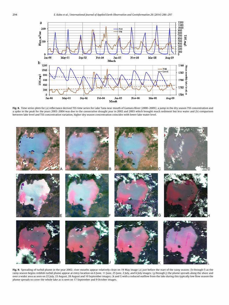
Fig. 8. Time series plots for (a) reflectance derived TSS time series for Lake Tana near mouth of Gumara River (2000–2009); a jump in the dry season TSS concentration anda spike in the peak for the years 2003–2004 was due to the consecutive drought year in 2002 and 2003 which brought much sediment but less water and (b) comparisonbetween lake level and TSS concentration variation, higher dry season concentration coincides with lower lake water level.

Fig. 9. Spreading of turbid plume in the year 2002; river mouths appear relatively clean on 19 May image (a) just before the start of the rainy season; (b through f) as therainy season begins reddish turbid plume appear at entry location on 6 June, 11 June, 25 June, 2 July, and 6 July images; (g through j) the plume spreads along the shore andover a wider area as seen on 22 July, 23 August, 28 August and 10 September images; (k and l) with a reduced outflow from the lake during this typically low flow season theplume spreads to cover the whole lake as is seen on 17 September and 9 October images.

E. Kaba et al. / International Journal of Applied Earth Observation and Geoinformation 26 (2014) 286–297 295

Fig. 10. 2000–2009 mean monthly reflectance-derived TSS (mg l−1) at river mouth depicting the annual cycle of alteration in the water clarity are constructed using theSURFER software.

2 th Obs

iog

lwtiflbwtosso2trbgctitTTl

iaftaf2trtoaca(mc

5

bwsrTohacdwMhtt

96 E. Kaba et al. / International Journal of Applied Ear

ncreased from 100 to 250 mg l−1 after 2002 due to a combinationf late wet season flows and apparent withdrawal for hydropowereneration.

The occurrence of TSS peak before flow peak is attributed to theoose soil condition at the start of the rainy season that is easily

ashed off and the suspended solids concentrations go up beforehe rainy season progresses. Recent field measurements on exper-mental watersheds in the Blue Nile showed that the subsurfaceow is negligible at the onset of the rainy season and the soil erodi-ility is the greatest because the soil is dry and loose. Once theatershed is saturated (i.e. the hill slopes are contributing water to

he stream), the sediment concentration in the water is a functionf the surface runoff and interflow components hence a decline inediment concentrations are observed toward the end of the rainyeason (Steenhuis et al., 2009). Same observations are reported byther studies made in the Ethiopian highlands (Bewket and Sterk,003; Descheemaeker et al., 2006; Tilahun et al., 2012). In contrast,he runoff coefficient and discharge are small in the beginning of theain and increase to the end of July where after the runoff coefficientecomes nearly constant (Liu et al., 2008). As the rainy season pro-resses, the soil becomes more cohesive and ground water begins toontribute to stream flow, further diluting the sediment concentra-ion. TSS estimates from the regression equation are much smallern comparison to data from a rating curve. During the rainy seasonhe river overflows its banks downstream of the gauging station.he river gradient at this reach is so small that flow velocity is low.he flood water then spreads to the plain damping the sedimentoad. Consequently, relatively less turbid water reaches the lake.

The change in the dry season concentration at the end of the yearn 2002 coincides with the consecutive drought years (2002–2003)nd as a consequence the lowering of the lake by about two metersrom the long term mean. In this time, the dry season TSS concen-ration shifted from about 100 mg l−1 to 250 mg l−1 (Fig. 7(a)). With

much reduced outflow during low water levels the residence timeor the water, which is three years in normal seasons (Kebede et al.,006), will increase considerably. This facilitates further mixing ofhe turbid plume with the lake water. Successive images collectedight at the beginning of the rainy season show the spreading ofhe plume over the larger part of the lake. Thus, when the floodf the following season reaches the lake, the TSS concentration islready at a higher TSS level and hence the TSS extraction processatches this phenomenon resulting in TSS peaks for the years 2003nd 2004 (Fig. 7(b)). Satellite images of May through October 2002Fig. 9) are used to show how the plume spreads over the lake. The

ean monthly TSS map at the river mouth is overlain with TSSontour lines (Fig. 10).

. Conclusion

Unlike discharge data, which are measured generally on a dailyasis, sediment concentration data often result from infrequentater quality monitoring campaigns. A robust statistical relation-

hip was constructed between TSS, turbidity and Secchi depth andemotely sensed reflectance at the entry location of Gumara River.he established regression equations can be used to provide syn-ptic water quality at the river entry and hence helps to assessow soil and water conservation investments pay dividends. Thevailability of MODIS images on an almost daily basis provides theapability to monitor sediment inflow dynamics especially in thery season and during the beginning of the rainy season, duringhich the peak of the sediment arrives the lake. Thus, the use of

ODIS images in TSS and turbidity measurement supersedes the

igher spatial resolution images in (e.g. Landsat ETM+, ASTER) dueo much higher temporal resolution. MODIS images also providehe advantage of increased sensitivity (Hu et al., 2004).

ervation and Geoinformation 26 (2014) 286–297

The regression equations may also be applied to adjacent water-sheds feeding Lake Tana that have similar soils and geologicalformations, as these are expected to have similar particle size char-acteristics and hence similar reflectance characteristics (Horsburghet al., 2010). However the transferability of the regression equationsdeveloped here should be verified. Thus, similar regression equa-tions have to be established for other major contributing rivers,at minimum with a validation sampling campaign and possiblyincluding more training sampling campaigns. The work is impor-tant enough to consider extending the regression equations tocover the whole lake. Time series TSS generated from the estab-lished regression equations can then be used to calculate an annualinflow and outflow sediment budget and then estimate loss of lakestorage capacity. However the estimation of total suspended solidswithin the lake requires profiling vertical TSS concentrations atrepresentative sites, or making defensible assumptions regardingthe vertical distribution (Li et al., 2003). The correlation betweenmeasured TSS and total sediment, once established, can be usedto determine the total inflowing sediment. The knowledge of TSShas great importance in modeling the inflow of nutrients and con-taminants which has implications for eutrophication, algal bloomsand degradation of aquatic habitat (Smith, 2008). A better under-standing of the movement of the turbid plume can also be used inhydrodynamic modeling of the lake.

Acknowledgments

USDA-SRE and the HED provided partial support for thisresearch. Bahir Dar Fishery and Aquatic Life Research Centre(BFALRC) and Tana Sub Basin Office (TaSBO) at Bahir Dar pro-vided logistic support in the data collection campaigns. The authorswould also like to thank the two anonymous reviewers for theirconstructive comments.

References

Ayana, E.K., 2007. Validation Of Radar Altimetry Lake Level Data And It’s ApplicationIn Water Resources Management. University of Twente, The Netherland, MasterThesis.

Baban, S.M., 1993. Detecting water quality parameters in the Norfolk Broads, UK,using Landsat imagery. International Journal of Remote Sensing 14, 1247–1267.

Betru, N., Sonali, W., 2010. Disaster risk reduction: experience from the MERETproject in Ethiopia. In: Steven Were Omamo, U.G.a.S.S. (Ed.), Revolution: FromFood Aid to Food Assistance. WFP, Rome, pp. 139–156.

Bewket, W., Sterk, G., 2003. Assessment of soil erosion in cultivated fields using asurvey methodology for rills in the Chemoga watershed, Ethiopia. Agriculture,Ecosystems & Environment 97, 81–93.

Bi, N., Yang, Z., Wang, H., Fan, D., Sun, X., Lei, K., 2011. Seasonal variation ofsuspended-sediment transport through the southern Bohai Strait. Estuarine,Coastal and Shelf Science 93, 239–247.

Chami, M., Marken, E., Stamnes, J., Khomenko, G., Korotaev, G., 2006. Variabilityof the relationship between the particulate backscattering coefficient and thevolume scattering function measured at fixed angles. Journal of GeophysicalResearch: Oceans 111, 1978–2012.

Chen, Z., Hu, C., Muller-Karger, F., 2007. Monitoring turbidity in Tampa Bay usingMODIS/Aqua 250-m imagery. Remote Sensing of Environment 109, 207–220.

Dall’Olmo, G., Gitelson, A.A., Rundquist, D.C., Leavitt, B., Barrow, T., Holz, J.C., 2005.Assessing the potential of SeaWiFS and MODIS for estimating chlorophyll con-centration in turbid productive waters using red and near-infrared bands.Remote Sensing of Environment 96, 176–187.

Delmas, M., Cerdan, O., Cheviron, B., Mouchel, J.-M., 2011. River basin sediment fluxassessments. Hydrological Processes 25, 1587–1596.

Descheemaeker, K., Nyssen, J., Rossi, J., Poesen, J., Haile, M., Raes, D., Muys, B., Moey-ersons, J., Deckers, S., 2006. Sediment deposition and pedogenesis in exclosuresin the Tigray Highlands, Ethiopia. Geoderma 132, 291–314.

Doxaran, D., Froidefond, J.-M., Lavender, S., Castaing, P., 2002. Spectral signature ofhighly turbid waters: application with SPOT data to quantify suspended partic-ulate matter concentrations. Remote Sensing of Environment 81, 149–161.

Froidefond, J.-M., Castaing, P., Prud’homme, R., 1999. Monitoring suspended partic-

ulate matter fluxes and patterns with the AVHRR/NOAA-11 satellite: applicationto the Bay of Biscay, Deep Sea Research Part II. Topical Studies in Oceanography46, 2029–2055.

Gadgil, A., 1998. Drinking water in developing countries. Annual Review of Energyand the Environment 23, 253–286.

th Obs

G

G

G

H

H

H

H

H

H

H

H

J

K

K

K

L

L

L

L

L

M

M

M

E. Kaba et al. / International Journal of Applied Ear

ebeyehu, A., 2004. The role of large water reservoirs. In: 2nd International Confer-ence on the Ethiopian Economy.

etis, A., Ord, J.K., 2010. The analysis of spatial association by use of distance statis-tics. In: Perspectives on Spatial Data Analysis. Springer, Berlin Heidelberg, pp.127–145.

üttler, F.N., Niculescu, S., Gohin, F., 2013. Turbidity retrieval and monitoring ofDanube Delta waters using multi-sensor optical remote sensing data: an inte-grated view from the delta plain lakes to the western–northwestern Black Seacoastal zone. Remote Sensing of Environment 132, 86–101.

aileslassie, A., Priess, J., Veldkamp, E., Teketay, D., Lesschen, J.P., 2005. Assessmentof soil nutrient depletion and its spatial variability on smallholders’ mixed farm-ing systems in Ethiopia using partial versus full nutrient balances. Agriculture,Ecosystems & Environment 108, 1–16.

an, L., 2005. Estimating chlorophyll-a concentration using first-derivative spectrain coastal water. International Journal of Remote Sensing 26, 5235–5244.

an, L., Rundquist, D.C., 1994. The response of both surface reflectance and theunderwater light field to various levels of suspended sediments: preliminaryresults. Photogrammetric Engineering and Remote Sensing 60, 1463–1471.

aregeweyn, N., Poesen, J., Nyssen, J., De Wit, J., Haile, M., Govers, G., Deckers, S.,2006. Reservoirs in Tigray (Northern Ethiopia): characteristics and sedimentdeposition problems. Land Degradation & Development 17, 211–230.

ashimoto, K., Oki, K., 2012. Estimation of discharges at river mouth with MODISimage. International Journal of Applied Earth Observation and Geoinformation.

erweg, K., Ludi, E., 1999. The performance of selected soil and water conservationmeasures—case studies from Ethiopia and Eritrea. Catena 36, 99–114.

orsburgh, J.S., Spackman Jones, A., Stevens, D.K., Tarboton, D.G., Mesner, N.O., 2010.A sensor network for high frequency estimation of water quality constituentfluxes using surrogates. Environmental Modelling & Software 25, 1031–1044.

u, C., Chen, Z., Clayton, T.D., Swarzenski, P., Brock, J.C., Muller-Karger, F.E.,2004. Assessment of estuarine water-quality indicators using MODIS medium-resolution bands: Initial results from Tampa Bay, FL. Remote Sensing ofEnvironment 93, 423–441.

olivet, D., Ramon, D., Deschamps, P.-Y., Steinmetz, F., Fougnie, B., Henry, P., 2007.How the ocean color product quality is limited by atmospheric correction. In:Envisat. Proc. Symposium.

aufman, Y.J., Herring, D.D., Ranson, K.J., Collatz, G.J., 1998. Earth observing systemAM1 mission to earth. IEEE Transactions on Geoscience and Remote Sensing 36,1045–1055.

ebede, S., Travi, Y., Alemayehu, T., Marc, V., 2006. Water balance of Lake Tanaand its sensitivity to fluctuations in rainfall, Blue Nile basin, Ethiopia. Journalof Hydrology 316, 233–247.

utser, T., Metsamaa, L., Vahtmäe, E., Strömbeck, N., 2006. Suitability of MODIS250 m resolution band data for quantitative mapping of cyanobacterial blooms.Estonian Academy of Sciences Proceedings Biology Ecology 55, 318–328.

i, R.-R., Kaufman, Y.J., Gao, B.-C., Davis, C.O., 2003. Remote sensing of suspendedsediments and shallow coastal waters. IEEE Transactions on Geoscience andRemote Sensing 41, 559–566.

ind, O.T., Doyle, R., Vodopich, D.S., Trotter, B.G., Gualberto Limón, J., Davalos-Lind, L.,1992. Clay turbidity: regulation of phytoplankton production in a large, nutrient-rich tropical lake. Limnology and Oceanography 37, 549–565.

iu, Y., Islam, M.A., Gao, J., 2003. Quantification of shallow water quality parametersby means of remote sensing. Progress in Physical Geography 27, 24–43.

iu, B.M., Collick, A.S., Zeleke, G., Adgo, E., Easton, Z.M., Steenhuis, T.S., 2008. Rainfall-discharge relationships for a monsoonal climate in the Ethiopian highlands.Hydrological Processes 22, 1059–1067.

iu, D., Fu, D., Xu, B., Shen, C., 2012. Estimation of total suspended matter inthe Zhujiang (Pearl) River estuary from Hyperion imagery. Chinese Journal ofOceanology and Limnology 30, 16.

a, R., Dai, J., 2005. Investigation of chlorophyll-a and total suspended matter con-centrations using Landsat ETM and field spectral measurement in Taihu Lake,China. International Journal of Remote Sensing 26, 2779–2795.

ao, Z., Chen, J., Pan, D., Tao, B., Zhu, Q., 2012. A regional remote sensing algorithm

for total suspended matter in the East China Sea. Remote Sensing of Environment124, 819–831.

cCartney, M., Alemayehu, T., Shiferaw, A., Awulachew, S., 2010. Evaluation of cur-rent and future water resources development in the Lake Tana Basin. Ethiopia,Iwmi.

ervation and Geoinformation 26 (2014) 286–297 297

Miller, R.L., McKee, B.A., 2004. Using MODIS Terra 250 m imagery to map con-centrations of total suspended matter in coastal waters. Remote Sensing ofEnvironment 93, 259–266.

Min, J.-E., Ryu, J.-H., Lee, S., Son, S., 2012. Monitoring of suspended sediment variationusing Landsat and MODIS in the Saemangeum coastal area of Korea. MarinePollution Bulletin 64, 382–390.

Mitchell, A., 2005. GIS Analysis Volume 2: Spatial Measurements & Statistics. ESRIPress, Redlands, California.

Nechad, B., Ruddick, K., Park, Y., 2010. Calibration and validation of a generic mul-tisensor algorithm for mapping of total suspended matter in turbid waters.Remote Sensing of Environment 114, 854–866.

Nyssen, J., Poesen, J., Descheemaeker, K., Haregeweyn, N., Haile, M., Moeyersons, J.,Frankl, A., Govers, G., Munro, N., Deckers, J., 2008. Effects of region-wide soil andwater conservation in semi-arid areas: the case of northern Ethiopia. Zeitschriftfür Geomorphologie 52, 291–315.

Ord, J.K., Getis, A., 1995. Local spatial autocorrelation statistics: distributional issuesand an application. Geographical Analysis 27, 286–306.

Petus, C., Chust, G., Gohin, F., Doxaran, D., Froidefond, J.-M., Sagarminaga, Y., 2010.Estimating turbidity and total suspended matter in the Adour River plume(South Bay of Biscay) using MODIS 250-m imagery. Continental Shelf Research30, 379–392.

Smith, H.G., 2008. Estimation of suspended sediment loads and delivery in an incisedupland headwater catchment, south-eastern Australia. Hydrological Processes22, 3135–3148.

Spear, B., Smith, D., Largay, B., Haskins, J., 2008. In: Watson, F. (Ed.), Turbidity as aSurrogate Measure for Suspended Sediment Concentration in Elkhorn Slough.The Watershed Institute, California State University Monterey Bay, Seaside CA,p. 26.

Steenhuis, T.S., Collick, A.S., Easton, Z.M., Leggesse, E.S., Bayabil, H.K., White, E.D.,Awulachew, S.B., Adgo, E., Ahmed, A.A., 2009. Predicting discharge and sedi-ment for the Abay (Blue Nile) with a simple model. Hydrological Processes 23,3728–3737.

Tilahun, S., Guzman, C., Zegeye, A., Engda, T., Collick, A., Rimmer, A., Steenhuis,T., 2012. An efficient semi-distributed hillslope erosion model for the subhumid Ethiopian Highlands. Hydrology and Earth System Sciences Discussions9, 2121–2155.

Tilahun, S., Guzman, C., Zegeye, A., Engda, T., Collick, A., Rimmer, A., Steenhuis, T.,2013. An efficient semi-distributed hillslope erosion model for the subhumidEthiopian Highlands. Hydrology and Earth System Sciences 17, 1051–1063.

USGS, Surface Reflectance Daily L2G Global 250 m, in, 2011.Vijverberg, J., Sibbing, F.A., Dejen, E., 2009. Lake Tana: Source of the Blue Nile.

Springer, The Nile, pp. 163–192.Villar, R.E., Martinez, J.-M., Guyot, J.-L., Fraizy, P., Armijos, E., Crave, A., Bazán, H.,

Vauchel, P., Lavado, W., 2012. The integration of field measurements and satelliteobservations to determine river solid loads in poorly monitored basins. Journalof Hydrology.

Wang, J.J., Lu, X., 2010a. Estimation of suspended sediment concentrations usingTerra MODIS: An example from the Lower Yangtze River, China. Science of theTotal Environment 408, 1131–1138.

Wang, J.-J., Lu, X., 2010b. Estimation of suspended sediment concentrations usingTerra MODIS: an example from the Lower Yangtze River, China. Science of theTotal Environment 408, 1131–1138.

Wang, J.J., Lu, X.X., Liew, S.C., Zhou, Y., 2009. Retrieval of suspended sedi-ment concentrations in large turbid rivers using Landsat ETM+: an examplefrom the Yangtze River, China. Earth Surface Processes and Landforms 34,1082–1092.

Wang, J.-J., Lu, X.X., Liew, S.C., Zhou, Y., 2010. Remote sensing of suspended sedimentconcentrations of large rivers using multi-temporal MODIS images: an examplein the Middle and Lower Yangtze River, China. International Journal of RemoteSensing 31, 1103–1111.

Werdell, P.J., Franz, B.A., Bailey, S.W., 2010. Evaluation of shortwave infrared atmo-spheric correction for ocean color remote sensing of Chesapeake Bay. Remote

Sensing of Environment 114, 2238–2247.

Yilma, A.D., Awulachew, S.B., 2009. Blue Nile Basin Characterization and GeospatialAtlas, Improved Water and Land Management in the Ethiopian Highlands: ItsImpact on Downstream Stakeholders Dependent on the Blue Nile, 6. Intermedi-ate Results Dissemination Workshop, ILRI, Addis Ababa, Ethiopia, 5–6 February.