EVAL: Utilizing Processors with Variation-Induced Timing Errors ∗

Smruti Sarangi, Brian Greskamp, Abhishek Tiwari , andJosep TorrellasDepartment of Computer Science

University of Illinois at Urbana-Champaignhttp://iacoma.cs.uiuc.edu

AbstractParameter variation in integrated circuits causes sections of

a chip to be slower than others. If, to prevent any resulting tim-ing errors, we design processors for worst-case parameter values,we may lose substantial performance. An alternate approach ex-plored in this paper is to design for closer to nominal values, andprovide some transistor budget to tolerate unavoidable variation-induced errors.

To assess this approach, this paper first presents a novel frame-work that shows how microarchitecture techniques can tradeoff variation-induced errors for power and processor frequency.Then, the paper introduces an effective technique to maximizeperformance and minimize power in the presence of variation-induced errors, namelyHigh-Dimensionaldynamic adaptation.For efficiency, the technique is implemented using a machine-learning algorithm. The results show that our best configurationincreases processor frequency by 56% on average, allowing theprocessor to cycle 21% faster than without variation. Processorperformance increases by 40% on average, resulting in a per-formance that is 14% higher than without variation — at only a10.6% area cost.

1 IntroductionAs integrated circuit technology continues to scale, the next

major challenge faced by high-performance processor designersis parameter variation [30]: the fact that Process, Voltage, andTemperature (PVT) values change from their nominal specifica-tions. Designing processors under variation is harder because theyhave to work under a wide range of conditions.

One of the most harmful effects of variation is that some sec-tions of the chip are slower than others — either because theirtransistors are intrinsically slower or because temperature or sup-ply voltage conditions render them so. Logic paths in these sec-tions may take too long to propagate signals and, as a result, in-duce timing errors. On current trends, designers in upcomingtechnology generations may have to create overly conservativedesigns to avoid risking these errors. It has been suggested thatparameter variation may wipe out a sizable fraction of the poten-tial gains of future technology generations [2].

An alternative scenario, which this paper explores, is that ina high-variability environment, cost-effective processors may bedesigned to tolerate errors due to parameter variation. In this case,

∗This work was supported by the National Science Foundation undergrant CPA-0702501 and by SRC GRC under grant 2007-HJ-1592. SmrutiSarangi is now with IBM India Software Laboratories, in Bangalore (sr-sarangi@in.ibm.com). Abhishek Tiwari is now with Goldman Sachs, inNew York City (abhishek.tiwari@gs.com).

processors may be designed not for worst-case parameter valuesbut for closer to nominal-case parameter values — and providesome transistor budget to tolerate the resulting variation-inducederrors. The result may be a higher-performing processor and/or acheaper manufacturing process — in short, a more cost-effectivedesign.

To explore this scenario, it is first necessary to consider how pa-rameter variation induces timing errors in high-performance pro-cessors. Second, while we could reuse existing fault-tolerant ar-chitectures to handle these errors, it is important to understandhow the rate of these errors can be traded-off for other quanti-ties, such as processor power or frequency. Finally, we need toidentify microarchitecture techniques that minimize such errors,possibly also affecting the power and frequency of the processor.This paper addresses the last two challenges and makes two con-tributions.

First, it introduces a novel framework called EVAL (Environ-ment for Variation-Afflicted Logic) to understand how processorscan tolerate and mitigate variation-induced errors. In EVAL, mi-croarchitecture techniques can trade off error rate for power andprocessor frequency.

Second, this paper presentsHigh-Dimensionaldynamic adap-tation, an effective microarchitecture technique to maximize pro-cessor performance and minimize power in the presence ofvariation-induced timing errors. The parameters adapted includethe processor frequency, multiple voltages, and two processorstructures. To efficiently support this technique, we propose animplementation based on machine learning.

Our results show that, under variation-induced timing errors,high-dimensional dynamic adaptation is feasible and effective.With no support for handling variation, a processor can only cy-cle at 78% of its no-variation frequency. However, by dynami-cally adapting processor frequency, per-subsystem voltages, issuequeue size, and functional-unit structure, the processor increasesits frequency by 56% on average — effectively cycling 21% fasterthan under no variation. Processor performance increases by 40%on average (or 14% over the no-variation scenario), always withinerror-rate, power, and temperature constraints. The area overheadof this technique is only 10.6% of the processor area.

This paper is organized as follows. Section 2 gives a back-ground; Section 3 presents the EVAL framework; Section 4 de-scribes high-dimensional dynamic adaptation and its implemen-tation; Sections 5–6 evaluate it; and Section 7 discusses relatedwork.

# of

Dyn

Pat

hs

var

T nom T var EE

rror

Rat

e (P

) E

Err

or R

ate

(P

)

f nom

(c)

Delay

nomT

(a) (b)

Delay

ft

1

(d)

Frequency

Frequency

Stage 1Stage 2

Processor

# of

Dyn

Pat

hsf

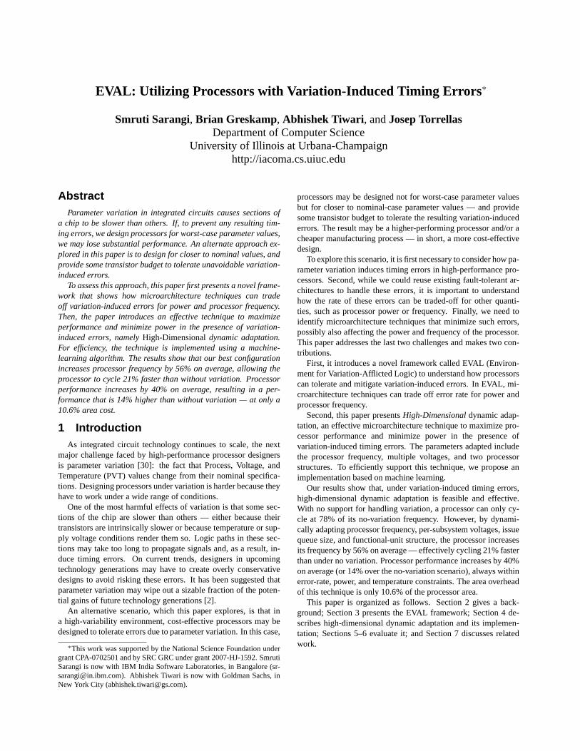
Figure 1:Impact of variation on processor frequency.

2 Background2.1 Modeling Process Variation

While process variation exists at several levels, we focus onWithin-Die (WID) variation, which is caused by bothsystematiceffects due to lithographic irregularities andrandomeffects, pri-marily due to varying dopant concentrations [30]. Two importantprocess parameters affected by variation are the threshold volt-age (Vt) and the effective channel length (Leff ). Variation ofthese two parameters directly affects a gate’s delay (Tg) [25] anda gate’s static power from subthreshold leakage (Psta). These twomeasures plus a gate’s dynamic power (Pdyn) are given by:

Tg ∝ VddLeff

µ(Vdd − Vt)α(1)

Psta ∝ VddT 2e−qVt/kT (2)

Pdyn ∝ CV 2ddf (3)

whereVdd, T, C, and f are the supply voltage, temperature, ca-pacitance, and frequency, respectively, whileµ andα are processparameters andq andk are physical constants.

To model process variation, we use the model in [26]. In thismodel, the systematic component ofVt’s variation is modeledwith two parameters:σsys andφ. A chip is divided into a grid.Each grid cell takes on a single value ofVt’s systematic compo-nent as given by a multivariate normal distribution with parame-tersµ=0 andσsys. Along with this, the systematic component ofVt is spatially correlated using a function that only depends on thedistance between two points — not on their position in the chipor on the direction of the line that connects them. Such a func-tion decreases to zero for a distanceφ calledrange. Intuitively,this means that at distanceφ, there is no correlation between thesystematic components ofVt for two transistors.Leff is mod-eled similarly with a differentσsys but the sameφ. Overall, withthis model, we can generate per-chip personalized maps of thesystematic components ofVt andLeff .

Random variation occurs at the much smaller granularity ofindividual transistors. Random variation is added analytically, asrandom values from a normal distribution withµ=0 andσran.

By combining the systematic and random components of vari-ation, we get the total variation. From here, using Equations 2and 1, we compute the variation in the static power and delay ofgates. Then, integration of the static power over the whole pro-cessor provides an estimate of the processor’s static power. Toestimate the processor’s frequency, we take the variation in gatedelay and, ideally, would apply it to the design files of a state-of-the-art processor. Since we do not have such files, we applythe gate delay variation to the models of critical path distributionsin pipeline stages with logic and with memory structures foundin [26]. From the resulting slowest critical paths, we estimate theprocessor frequency.

2.2 Modeling Variation-Induced Timing ErrorsProcess variation slows down some critical paths in a proces-

sor. As a result, the maximum frequency attainable by the proces-sor decreases. If we do not operate the processor at the resultinglow, safe frequency, the processor will suffer timing errors. To es-timate the rate of these timing errors as a function of the processorfrequency, we use the VATS model [26].

VATS considers the dynamic distribution of the delays of all theexercised paths in a pipeline stage. Without variation, such distri-bution may look like that in Figure 1(a). All paths take less thanthe nominal clock period (Tnom). Parameter variation changesgate delay (as per Equation 1), making some paths faster whileothers slower. The result is a more spread-out dynamic path de-lay distribution as in Figure 1(b). The processor now requires alonger clock period (Tvar) to operate without timing errors.

If a processor is clocked with a periodt < Tvar (Figure 1(b)),when the paths to the right oft are exercised, they may cause tim-ing errors. An alternate way to see this is by plotting the errorrate (or probability of errorPE) of the pipeline stage as we in-crease the pipeline frequency (Figure 1(c)). Forf > fvar, wherefvar=1/Tvar, there are errors.

VATS generates aPE(f) curve like the one in Figure 1(c) fora given pipeline stage. VATS then models ann-stage pipeline asa series failure system, where each stage can fail independently.Each stagei has an activity factorρi, which is the number oftimes that the average instruction exercises the stage. Finally, theprocessor error rate per instruction as a function of the frequencyf is given by Equation 4, and is shown in Figure 1(d) for a 2-stagepipeline.

PE(f) =

n∑i=1

(ρi × PEi(f)) (4)

2.3 Fine-Grain ABB and ASV ApplicationTwo techniques that modify the properties of gates are Adap-

tive Body Biasing (ABB) and Adaptive Supply Voltage (ASV).ABB [21, 35, 36] applies a body-bias voltageVbb between thesubstrate and the source (or drain) of transistors to either decreaseVt (Forward BB or FBB), or increaseVt (Reverse BB or RBB).As per Equations 1 and 2, decreasingVt reducesTg but increasesPsta; increasingVt causes the opposite behavior. ABB requiressome extra fabrication steps.

ASV changes theVdd applied to gates [5]. As per Equations 1,2 and 3, increasingVdd reducesTg but increasesPsta and, espe-cially, Pdyn; decreasingVdd causes the opposite behavior. ASVis simpler to implement than ABB.

A chip can have multiple ABB or ASV domains — an envi-ronment referred to as fine-grained. Tschanzet al. [35] built achip with 21 ABB domains. Narendraet al. [21] built a chip witha single ABB domain, although the chip includes 24 local biasgenerators with separate local bias networks — just as would berequired in an implementation with domains. Both sets of authorsestimate that the area overhead of their ABB support is≈2%.

2f

(e)(d)

f ff optf varf var f var f var f var f f

(b) (c)

After After

Perf

Perf

orm

ance

(Pe

rf)

(a)

Frequency

EEEE

rror

Rat

e (P

)

Err

or R

ate

(P

)

Err

or R

ate

(P

)

EE

rror

Rat

e (P

)

Before

EE

rror

Rat

e (P

) ReshapeTilt Shift Adapt

Frequency

Before Before

Frequency Frequency Frequencyf

AfterPE

1 nom

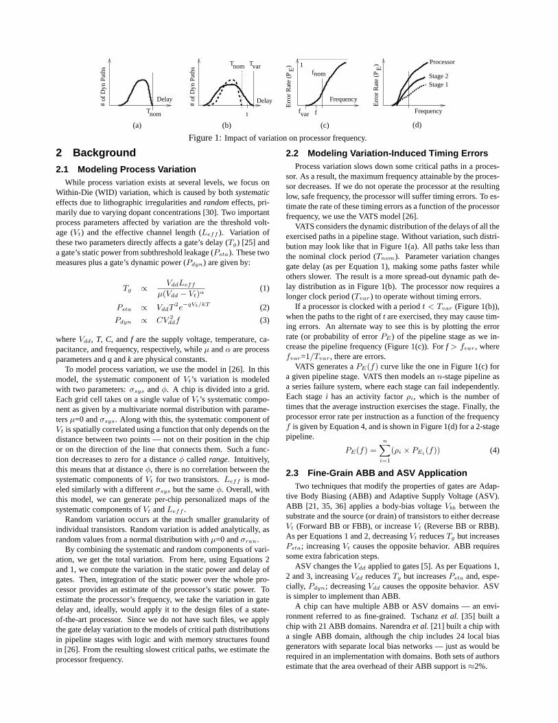
Figure 2:Tolerating (a) and mitigating (b)-(e) variation-induced errors in the EVAL framework.

If we assume that ASV supplies are chip-external, the areaoverhead of multiple ASV domains is small. Existing power sup-ply pins are repurposed to deliver customizedVdd levels to eachdomain. Then, level converters may need to be added to crossvoltage domains.

In this paper, we will initially assume that we can support over10 ABB and ASV domains in a processor pipeline. While thisis a stretch with current technology, current research (e.g., [15])points to promising directions to make it feasible. We will thensee that we do not need as much support.

3 The EVAL FrameworkWe assume that, in a high-variability environment, cost-

effective processors will not be slowed down to operate at worst-case parameter values — their performance atTvar is low. In-stead, we assume that they will be clocked with a periodt < Tvar

(Figure 1(b)) and suffer timing errors during normal execution.To design cost-effective processors in this challenging environ-

ment, we propose the EVAL framework to tolerate and mitigatevariation-induced errors. In EVAL, microarchitecture techniquescan trade-off error rate for power and processor frequency.

3.1 Tolerating ErrorsIf we augment the processor with support for error detection

and correction, it is possible to cycle the processor atf > fvar

while still ensuring correct execution. For instance, we can add achecker unit like Diva [40] to verify results from the main pipelineat instruction retirement. To ensure that the checker is error-free,it can be clocked at a safe, lower frequency than the main core,while the speed of its transistors is enhanced with ABB or ASV(Section 2.3) — according to [40], it is feasible to design a wide-issue checker thanks to its architectural simplicity. Alternately,we can add a checker processor like in Paceline [9], or augmentthe pipeline stages or functional units with error checking hard-ware like in a variety of schemes (e.g., [8, 37, 38]). With any ofthese architectures, the performance in instructions per second ofthe processor cycling atf is:

Perf(f) =f

CPI=

f

CPIcomp + CPImem + CPIrec

=f

CPIcomp + mr ×mp(f) + PE(f)× rp(5)

where, for the average instruction,CPIcomp are the computationcycles (including L1 misses that hit in the on-chip L2);CPImem

are stall cycles due to L2 misses; andCPIrec are cycles lost torecovery from timing errors. In addition,mr is the L2 miss ratein misses per instruction,mp is the observed L2 miss penalty incycles non-overlapped with computation,PE is the error rate perinstruction, andrp is the error recovery penalty in cycles.

To a first approximation,CPIcomp, mr, and rp remain con-stant as we changef. If we use a Diva-like scheme,rp is equal to

the branch misprediction penalty, since recovery involves takingthe result from the checker, flushing the pipeline, and restartingit from the instruction that follows the faulty one. On the otherhand, bothmpandPE increase withf.

For smallf, PE is small (Figure 1(c)), which makesPE × rpsmall. Consequently, asf increases,Perf goes up because the nu-merator grows while the denominator increases only slowly —driven by the second and third terms. Eventually, asf keeps in-creasing,PE reaches a point of fast growth, as shown in Fig-ure 1(c). At this point,PE × rp swells, andPerf levels off andquickly dips down. The result is shown in Figure 2(a), whichshows thePerf(f) curve with a solid line and thePE(f) curve indashes. We callfopt the f at the peakPerf. With this approach,we reach frequencies higher thanfvar by tolerating errors.

3.2 Mitigating Errors: Taxonomy of TechniquesWe can reduce the number of variation-induced errors with mi-

croarchitectural techniques. We group such techniques into fourclasses, depending on how they affect thePE vs f curve. In thissection, we describe the four classes — shown in Figures 2(b)-(e)— while in Section 3.3, we present one example of each class.

Tilt: This class of techniques speeds-up many paths that are al-most critical in a pipeline stage, but does not speed-up the slowestpaths in the stage. As a result, the slope of thePE vs f curvedecreases, but the point where the curve meets thef axis (fvar)remains unchanged (Figure 2(b)). Overall, for anf moderatelyhigher thanfvar, PE has decreased.

Shift: This class speeds-up all the paths in a stage by a similaramount. As a result, the curve largely shifts to the right (Fig-ure 2(c)), therefore reducingPE for a givenf .

Reshape: There is typically anenergy costin tilting or shift-ing the curve as just described. Consequently, another class oftechniques speeds-up the slow paths in the stage (thus consumingenergy) and then saves energy by slowing down the fast paths.The first action shifts the bottom of thePE vs f curve to the rightand/or reduces the curve’s initial slope; the second action shiftsthe top of the curve to the left and/or increases the curve’s finalslope (Figure 2(d)). For thef considered, the result is a lowerPE

with potentially little energy cost. In reality, it may be easier toobtain this behavior at the processor level by speeding-up slowpipeline stages and slowing down the fast stages.

Adapt: As an application executes, it changes the types of op-erations it performs. As a result, itsPE vs f curve also changes,as shown in Figure 2(e). A final class of techniques adapts thefof the processor dynamically, to keep it as high as possible whilemaintainingPE low at all times (Figure 2(e)).

3.3 Example of Error-Mitigation TechniquesWe now list one example of each of the four classes of tech-

niques to mitigate variation-induced errors.

3.3.1 Tilt: FU Replica without Critical-Path WallDesign tools often design pipeline stages or Functional Units

(FUs) with many near-critical paths. This is because, to save areaand power, the non-critical paths are not subjected to high opti-mization — as long as they are shorter than the critical path, theyare considered good enough. This creates a critical-path wall. Thetypical Tilt technique consists of taking a design and optimizingthe near-critical paths to be shorter, so that the distribution of pathdelays and, therefore, thePE vs f curve, become less steep. Onepossible way to do so is by increasing the width (W) of the tran-sistors in the non-critical paths. This decreases their delay, whichis proportional toK1 + K2/W. However, it also increases theirpower and area, since they are proportional toW [22].

Consequently, we propose to have two implementations of anFU side-by-side. Both contain the same logic circuit, but one isthe original design (Normal) and the other has the transistors inthe non-critical paths optimized (LowSlope). LowSlopeis lesspower-efficient, but it has a lower-slopedPE vs f curve. Con-sequently, if the pair of FUs falls on a chip area with fast transis-tors, since the FUs will not limit the processor frequency, we en-ableNormaland disableLowSlope— the processor will be morepower efficient. If the pair falls on an area with slow transistorsand limits the frequency of the processor, we enableLowSlopeand disableNormal — the processor will cycle at a higherf forthe samePE .

We implement this technique in the most critical (typically, thehottest) FUs: we replicate the integer ALU unit and, inside theFP unit, replicate the adder and multiplier. Due to the area im-plications discussed in Section 5, we conservatively add one ex-tra pipeline stage between the register file read and the executestages.

3.3.2 Shift: Resizable SRAM StructuresA technique that has been proposed for SRAMs such as caches

or queues is to dynamically disable sections of them to reducepower, access time or cycle time (e.g., [4]) — since smaller struc-tures are faster. In these schemes, transmission gates separatesections of the structure; disabling transmission gates reduces thestructure size. According to [4], SPICE simulations show that theimpact of properly-designed transmission gates on the cycle timeis negligible.

This is a possibleShift technique. On chips where the RAMstructure falls on a fast region, the whole structure is kept (Largedesign). On chips where it falls on a slow region and limits thechip’s f, we disable a fraction of the structure (Smalldesign). Withshorter buses to charge, most of the paths in the structure speed up,shifting thePE curve to the right. Consequently, at anyf, Small’sPE is lower thanLarge’s. A shortcoming is that downsizing maydecrease IPC. However, we now have room to trade morePE forhigherf and still come out ahead in performance.

We implement this technique in the integer and FP issuequeues, since they are often critical. We enable them to operate ateither full or3/4capacity.

3.3.3 Reshape: Fine-Grain ABB or ASVABB and ASV have been used to speed up slow sections of a

chip and reduce the power of fast sections of the chip (e.g., [31,36]). Using them in our framework reshapes thePE curve asin Figure 2(d): speeding-up the slow pipeline stages pushes thelower part of the curve to the right and reduces its initial slope;slowing down and saving power on the fast pipeline stages pushes

the upper part of the curve to the left and increases its final slope.

3.3.4 Dynamic AdaptationMany algorithms have been proposed to dynamically change

parameters such as voltage, frequency, or cache size to adapt toapplication demands (e.g., [6, 7, 10]). In the context of mitigatingWID parameter variation, the key difference is that the problemhas a veryhigh dimensionality. The reason is that, to be effective,we need to sense from and actuate on many chip localities — asmany as regions with different parameter values — and then opti-mize globally. Due to the complexity of the problem, we proposean implementation using machine learning algorithms; they en-able rapid adaptation in multiple dimensions with minimal com-putation cost.

High-dimensional dynamic adaptation is the key technique inEVAL, and the one that agglutinates all the other techniques. Wedescribe it next.

4 High-Dimensional DynamicAdaptation for Variation Errors

We proposeHigh-Dimensionaldynamic adaptation as a noveltechnique to effectively mitigate WID parameter variation in up-coming processor chips. The goal is to boost the processor fre-quency when there is room in the tolerablePE , power, andT.This technique involves (i) sensing from the several variation lo-calities, (ii) relying on local techniques totilt , shift, or reshapethePE vs f curve in each locality, and (iii) finally optimizing glob-ally. Given the complexity of the problem, we propose an im-plementation with asoftware-based fuzzycontroller. Every timethat a phase change is detected in the application, the processoris interrupted and runs the controller algorithm. The algorithmuses software data structures that contain fuzzy rules built by themanufacturer in a learning phase. In this section, we describe theproblem statement, the algorithm, and its implementation. As anexample, we adapt using all the example techniques described inSection 3.3, namely different ABB and ASV for each ofn pro-cessor subsystems, FU replication, and issue-queue resizing.

4.1 Optimization Problem StatementEvery optimization problem has a set of outputs subject to con-

straints, a final goal, and a set of inputs.Outputs. There are2n+3 outputs: (i) the core frequency, (ii) theVdd andVbb for each of then subsystems in the processor, (iii)the size of the issue queue (full or 3/4), and (iv) which FU to use(normal or low sloped). The last two outputs apply to integer orFP units depending on the type of application running.Constraints. There are three: (i) no point can be atT higher thanTMAX , (ii) the processor power cannot be higher thanPMAX ,and (iii) the total processorPE cannot be higher thanPEMAX .The reason for the latter is justified next.Goal. Our goal is to find the processorf that maximizes perfor-mance. However, taking Equation 5 and finding the point whereits derivative is zero is expensive. Instead, we can find a verysimilar f with little effort if our goal is to maximizef subject tothe processor’sPE being no higher thanPEMAX — assuming wechoose an appropriatePEMAX . Specifically, thePE(f) curve inFigure 2(a) is so steep that the range off betweenPE = 10−4 andPE = 10−1 errors/instruction is minuscule (only 2–3%). More-over, for typical values ofCPIcomp, CPImem, andrp in Equa-tion 5,PE = 10−4 makesCPIrec negligible, whilePE = 10−1

makesCPIrec so high thatPerf has already dropped. Conse-

MIN

f

fmax1

α1Vt01

thR1 ,,,K

sta1,K

dyn1

{ }f thRn Vt0

n αn,,,Kstan,K

dynn

{ f }

TH coref

α1Vt01

thR1 ,,,K

sta1,K

dyn1

{ }f thRn Vt0

n αn,,,Kstan,K

dynn

{ f }

VbbTH VbbV

ddV

ddn1 n1

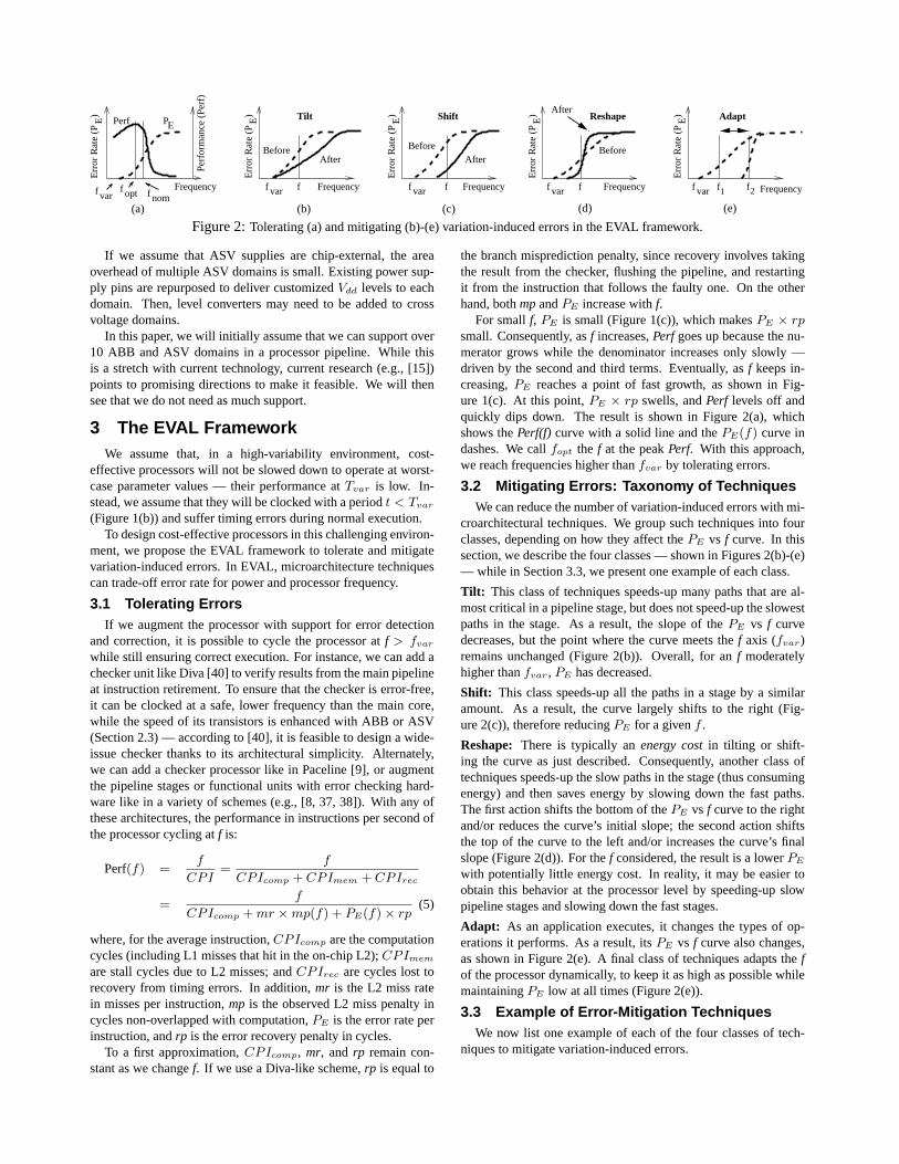
(a): Freq algorithm (b): Power algorithm

AlgorithmPowerPowerFreqFreq Algorithm Algorithm Algorithm

fmaxn

core

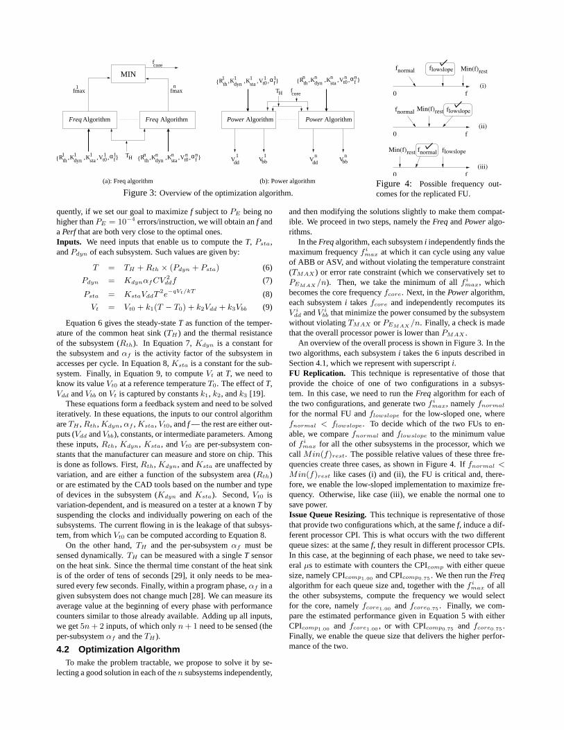
Figure 3:Overview of the optimization algorithm.

fnormal Min(f)rest

fnormalMin(f)rest flowslope

flowslope

fnormal flowslope Min(f)rest

(i)

(ii)

(iii)

f0

f0

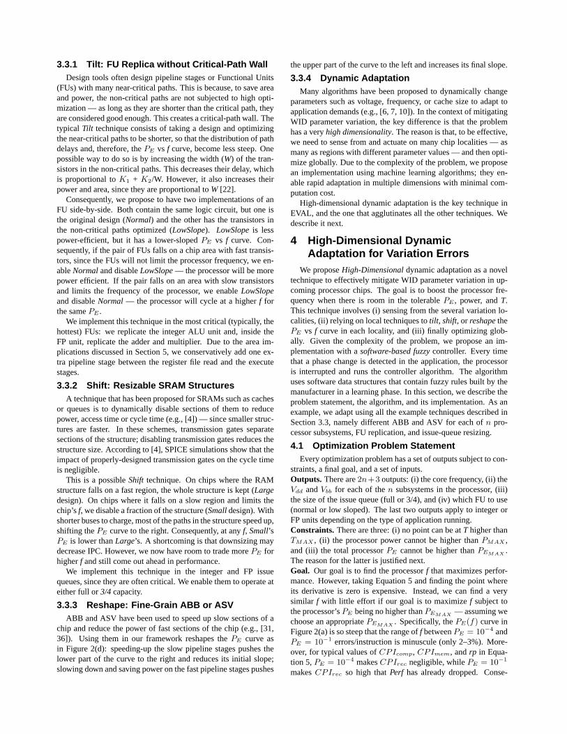
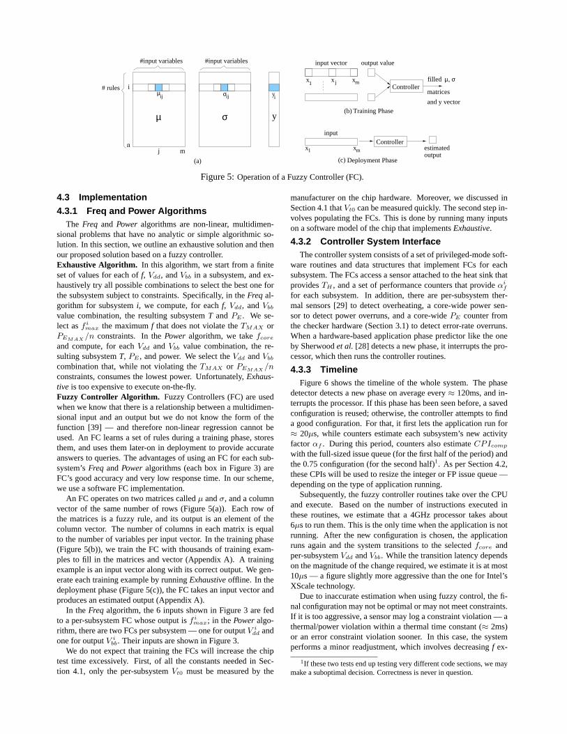
f0Figure 4: Possible frequency out-comes for the replicated FU.

quently, if we set our goal to maximizef subject toPE being nohigher thanPE = 10−4 errors/instruction, we will obtain anf andaPerf that are both very close to the optimal ones.Inputs. We need inputs that enable us to compute theT, Psta,andPdyn of each subsystem. Such values are given by:

T = TH + Rth × (Pdyn + Psta) (6)

Pdyn = KdynαfCV 2ddf (7)

Psta = KstaVddT 2e−qVt/kT (8)

Vt = Vt0 + k1(T − T0) + k2Vdd + k3Vbb (9)

Equation 6 gives the steady-stateT as function of the temper-ature of the common heat sink (TH ) and the thermal resistanceof the subsystem (Rth). In Equation 7,Kdyn is a constant forthe subsystem andαf is the activity factor of the subsystem inaccesses per cycle. In Equation 8,Ksta is a constant for the sub-system. Finally, in Equation 9, to computeVt at T, we need toknow its valueVt0 at a reference temperatureT0. The effect ofT,Vdd andVbb onVt is captured by constantsk1, k2, andk3 [19].

These equations form a feedback system and need to be solvediteratively. In these equations, the inputs to our control algorithmareTH , Rth, Kdyn, αf , Ksta, Vt0, andf — the rest are either out-puts (Vdd andVbb), constants, or intermediate parameters. Amongthese inputs,Rth, Kdyn, Ksta, andVt0 are per-subsystem con-stants that the manufacturer can measure and store on chip. Thisis done as follows. First,Rth, Kdyn, andKsta are unaffected byvariation, and are either a function of the subsystem area (Rth)or are estimated by the CAD tools based on the number and typeof devices in the subsystem (Kdyn and Ksta). Second,Vt0 isvariation-dependent, and is measured on a tester at a knownT bysuspending the clocks and individually powering on each of thesubsystems. The current flowing in is the leakage of that subsys-tem, from whichVt0 can be computed according to Equation 8.

On the other hand,TH and the per-subsystemαf must besensed dynamically.TH can be measured with a singleT sensoron the heat sink. Since the thermal time constant of the heat sinkis of the order of tens of seconds [29], it only needs to be mea-sured every few seconds. Finally, within a program phase,αf in agiven subsystem does not change much [28]. We can measure itsaverage value at the beginning of every phase with performancecounters similar to those already available. Adding up all inputs,we get5n + 2 inputs, of which onlyn + 1 need to be sensed (theper-subsystemαf and theTH ).

4.2 Optimization AlgorithmTo make the problem tractable, we propose to solve it by se-

lecting a good solution in each of then subsystems independently,

and then modifying the solutions slightly to make them compat-ible. We proceed in two steps, namely theFreq andPoweralgo-rithms.

In theFreqalgorithm, each subsystemi independently finds themaximum frequencyf i

max at which it can cycle using any valueof ABB or ASV, and without violating the temperature constraint(TMAX ) or error rate constraint (which we conservatively set toPEMAX /n). Then, we take the minimum of allf i

max, whichbecomes the core frequencyfcore. Next, in thePoweralgorithm,each subsystemi takesfcore and independently recomputes itsV i

dd andV ibb that minimize the power consumed by the subsystem

without violatingTMAX or PEMAX /n. Finally, a check is madethat the overall processor power is lower thanPMAX .

An overview of the overall process is shown in Figure 3. In thetwo algorithms, each subsystemi takes the 6 inputs described inSection 4.1, which we represent with superscripti.FU Replication. This technique is representative of those thatprovide the choice of one of two configurations in a subsys-tem. In this case, we need to run theFreq algorithm for each ofthe two configurations, and generate twof i

max, namelyfnormal

for the normal FU andflowslope for the low-sloped one, wherefnormal < flowslope. To decide which of the two FUs to en-able, we comparefnormal andflowslope to the minimum valueof f i

max for all the other subsystems in the processor, which wecall Min(f)rest. The possible relative values of these three fre-quencies create three cases, as shown in Figure 4. Iffnormal <Min(f)rest like cases (i) and (ii), the FU is critical and, there-fore, we enable the low-sloped implementation to maximize fre-quency. Otherwise, like case (iii), we enable the normal one tosave power.Issue Queue Resizing.This technique is representative of thosethat provide two configurations which, at the samef, induce a dif-ferent processor CPI. This is what occurs with the two differentqueue sizes: at the samef, they result in different processor CPIs.In this case, at the beginning of each phase, we need to take sev-eralµs to estimate with counters the CPIcomp with either queuesize, namely CPIcomp1.00 and CPIcomp0.75 . We then run theFreqalgorithm for each queue size and, together with thef i

max of allthe other subsystems, compute the frequency we would selectfor the core, namelyfcore1.00 andfcore0.75 . Finally, we com-pare the estimated performance given in Equation 5 with eitherCPIcomp1.00 and fcore1.00 , or with CPIcomp0.75 and fcore0.75 .Finally, we enable the queue size that delivers the higher perfor-mance of the two.

σ

µ σ ij yi

σ µfilled , 1

x xx j m

1j

(a)

# rules i

#input variables #input variables

nm

µ y

Controllermatrices

and y vector

input vector output value

x

inputController

xm estimated output

(b) Training Phase

(c) Deployment Phase

ij

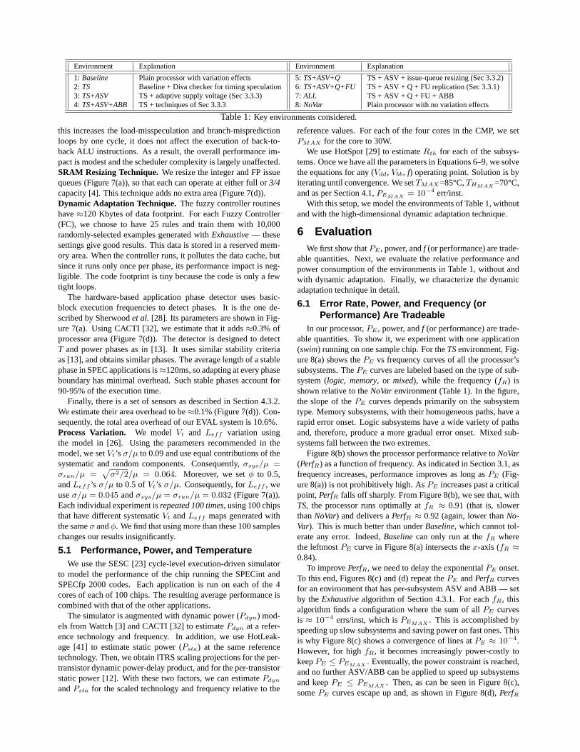
Figure 5:Operation of a Fuzzy Controller (FC).

4.3 Implementation4.3.1 Freq and Power Algorithms

The Freq and Power algorithms are non-linear, multidimen-sional problems that have no analytic or simple algorithmic so-lution. In this section, we outline an exhaustive solution and thenour proposed solution based on a fuzzy controller.Exhaustive Algorithm. In this algorithm, we start from a finiteset of values for each off, Vdd, andVbb in a subsystem, and ex-haustively try all possible combinations to select the best one forthe subsystem subject to constraints. Specifically, in theFreq al-gorithm for subsystemi, we compute, for eachf, Vdd, andVbb

value combination, the resulting subsystemT and PE . We se-lect asf i

max the maximumf that does not violate theTMAX orPEMAX /n constraints. In thePower algorithm, we takefcore

and compute, for eachVdd and Vbb value combination, the re-sulting subsystemT, PE , and power. We select theVdd andVbb

combination that, while not violating theTMAX or PEMAX /nconstraints, consumes the lowest power. Unfortunately,Exhaus-tive is too expensive to execute on-the-fly.Fuzzy Controller Algorithm. Fuzzy Controllers (FC) are usedwhen we know that there is a relationship between a multidimen-sional input and an output but we do not know the form of thefunction [39] — and therefore non-linear regression cannot beused. An FC learns a set of rules during a training phase, storesthem, and uses them later-on in deployment to provide accurateanswers to queries. The advantages of using an FC for each sub-system’sFreq andPoweralgorithms (each box in Figure 3) areFC’s good accuracy and very low response time. In our scheme,we use a software FC implementation.

An FC operates on two matrices calledµ andσ, and a columnvector of the same number of rows (Figure 5(a)). Each row ofthe matrices is a fuzzy rule, and its output is an element of thecolumn vector. The number of columns in each matrix is equalto the number of variables per input vector. In the training phase(Figure 5(b)), we train the FC with thousands of training exam-ples to fill in the matrices and vector (Appendix A). A trainingexample is an input vector along with its correct output. We gen-erate each training example by runningExhaustiveoffline. In thedeployment phase (Figure 5(c)), the FC takes an input vector andproduces an estimated output (Appendix A).

In the Freq algorithm, the 6 inputs shown in Figure 3 are fedto a per-subsystem FC whose output isf i

max; in thePoweralgo-rithm, there are two FCs per subsystem — one for outputV i

dd andone for outputV i

bb. Their inputs are shown in Figure 3.We do not expect that training the FCs will increase the chip

test time excessively. First, of all the constants needed in Sec-tion 4.1, only the per-subsystemVt0 must be measured by the

manufacturer on the chip hardware. Moreover, we discussed inSection 4.1 thatVt0 can be measured quickly. The second step in-volves populating the FCs. This is done by running many inputson a software model of the chip that implementsExhaustive.

4.3.2 Controller System InterfaceThe controller system consists of a set of privileged-mode soft-

ware routines and data structures that implement FCs for eachsubsystem. The FCs access a sensor attached to the heat sink thatprovidesTH , and a set of performance counters that provideαi

f

for each subsystem. In addition, there are per-subsystem ther-mal sensors [29] to detect overheating, a core-wide power sen-sor to detect power overruns, and a core-widePE counter fromthe checker hardware (Section 3.1) to detect error-rate overruns.When a hardware-based application phase predictor like the oneby Sherwoodet al. [28] detects a new phase, it interrupts the pro-cessor, which then runs the controller routines.

4.3.3 TimelineFigure 6 shows the timeline of the whole system. The phase

detector detects a new phase on average every≈ 120ms, and in-terrupts the processor. If this phase has been seen before, a savedconfiguration is reused; otherwise, the controller attempts to finda good configuration. For that, it first lets the application run for≈ 20µs, while counters estimate each subsystem’s new activityfactor αf . During this period, counters also estimateCPIcomp

with the full-sized issue queue (for the first half of the period) andthe 0.75 configuration (for the second half)1. As per Section 4.2,these CPIs will be used to resize the integer or FP issue queue —depending on the type of application running.

Subsequently, the fuzzy controller routines take over the CPUand execute. Based on the number of instructions executed inthese routines, we estimate that a 4GHz processor takes about6µs to run them. This is the only time when the application is notrunning. After the new configuration is chosen, the applicationruns again and the system transitions to the selectedfcore andper-subsystemVdd andVbb. While the transition latency dependson the magnitude of the change required, we estimate it is at most10µs — a figure slightly more aggressive than the one for Intel’sXScale technology.

Due to inaccurate estimation when using fuzzy control, the fi-nal configuration may not be optimal or may not meet constraints.If it is too aggressive, a sensor may log a constraint violation — athermal/power violation within a thermal time constant (≈ 2ms)or an error constraint violation sooner. In this case, the systemperforms a minor readjustment, which involves decreasingf ex-

1If these two tests end up testing very different code sections, we maymake a suboptimal decision. Correctness is never in question.

DTLB

FPQ

FPReg

LdStQ

Subsystem

Dcache

FPUnit

memory

memory

mixed

logic

memory

mixed

FPMap memory

IntALU logic

Type

ABB:From 2.4GHz to over 4GHz in 100MHz stepsFrom −500mV to 500mV in 50mV steps

From 800mV to 1200mV in 50mV stepsASV:

f:

MAX MAX H_MAX E_MAX

−4P =30W/proc, T =85C, T =70C, P =10 err/inst

IntReg

IntQ

IntMap

ITLB

memory

mixed

memory

memoryIcache memory

BranchPred mixed

Decode logic

(a): Some parameter values

(b): Subsystems used

(c): Logical organization of the checker

Checker 7.0

IntALU Repl

FPAdd/Mul Repl

I−Queue Resize 0.0

Phase Detector 0.3

Sensors 0.1

Total

CacheL1 I

CacheL1 D

Checker

Instr. QueueProcessor

Lower, Error−FreeFrequency

Core

L0 CachesParameter changes

Round trip latency in cycles from processor to:L1: 2; L2: 8; Memory: 208

IntALU subsystem (3 add/shift + 1 mult): 0.55% proc area1 FPadd + 1 FPmult: 1.90% proc area

Fuzzy controller system:Each FC: 25 rules; 10,000 training examplesPhase detector: 32 buckets; 6 bits/bucket

Process parameters:

Number of chips per experiment: 100

0.7

2.5

10.6

(d): Additional area

Area (% Proc)Source

0.0ASV

µ σ/µ φLeff: : 0.5 x Vt’sσ/µVt: : 150mV at 100C; : 0.09; : 0.5

σ/µ; :0.5φ

4−core CMP; Tech: 45nm; Vdd: 1V; f (no variation): 4GHz

Area measured from die photo:

Full−sized issue queues:Integer: 68 entriesFP: 32 entries

Figure 7:Characteristics of the system modeled.

10 µs

t

Heat sink cycle

Phase Phase

6 µs

0.5 µsNewMove 1 step

Bring to chosen working point

Measure

Retuning cycles

2−3 s

20 µs 2 ms 2 ms

Run fuzzy controller algorithm

compTest CPI for the 2 queue configurations

120 ms

αf for each subsystem

phasedetected

Figure 6:Timeline of the adaptation algorithm.

ponentially — first by 1 100MHz step, then by 2 steps, 4, and8 without running the controller — until the configuration causesno violation, and then gradually ramping upf in constant 100MHzsteps up until right below af that causes violations.

These smallf changes to prevent violations are calledRetun-ing Cycles(Figure 6). They donot involve re-running the fuzzycontroller. Finally, every 2–3s, theTH sensor is refreshed.

4.3.4 Summary of ComplexityWe believe that the complexity of this technique is modest. The

key part of the technique, namely the controller, is implementedin software, which reduces design complexity. The hardware as-pects include sensors, FU replication, issue-queue resizing, Divachecker, and fine-grain ABB/ASV. Note that this is not an “all-or-nothing” system — different subsets of techniques can be used.Finally, fuzzy control has been shown to be a simple, effectiveway to handle complicated control systems [39].

5 Evaluation EnvironmentWe model a Chip Multiprocessor (CMP) at 45nm technology

with four 3-issue cores similar to the AMD Athlon 64. Each corehas two 64KB L1 caches, a private 1MB L2, and hyper-transport

links to the other cores. We estimate a nominal (i.e., withoutvariation) frequency of 4GHz with a supply voltage of 1V. Fig-ure 7(a) shows some characteristics of the architecture. In thisevaluation, we choose to have 15 subsystems per core, as shownin Figure 7(b).

The frequency changes like in Intel XScale, and all changescan be effected in 10µs. Vbb andVdd can be adjusted on a per-subsystem basis, as in [36]. Figure 7(a) shows the ranges and stepsizes of the changes. Based on [21, 35], we estimate that the areaoverhead of ABB is≈ 2%. However, we will not include ABBin our preferred configuration. As indicated in Section 2.3, weoptimistically assume that the area overhead of ASV is largelynegligible [5], given chip-external ASV supplies. We will includeASV in our preferred configuration.

Each core has a checker like Diva [40] to detect and toleratecore errors (Figure 7(c)). The checker is sped up with ASV so thatit runs at 3.5GHz without any errors. It has a 4KB L0 D-cache,a 512B L0 I-cache, and a 32-entry queue to buffer instructionsretiring in the processor. To ensure that the checker reads the L1reliably, the L1 is augmented with the SRAM Razor scheme [14],which adds duplicate sense amplifiers to L1. L1 reads are per-formed with speculative timing for the core, and then a fraction ofa cycle later with safe timing for the checker. Since checker de-sign is not our contribution, we do not elaborate further, althoughwe include its area and power cost in our overall computations.FU Replication Technique. We replicate the integer ALU unitand, inside the FP unit, replicate the set composed of adder andmultiplier. To estimate the area, power, and timing of low-slopedFUs, we use the data in [1]. Although their circuit is a smallsequential circuit rather than an ALU, we consider that their mea-surements are an acceptable estimation of this optimization’s im-pact. On average, the low-sloped unit consumes 30% more areaand power, and its path delay distribution changes such that themean decreases by 25% and the variance doubles [1]. From this,and the FU area shown in Figure 7(a), it follows that integer andFP FU replication adds 0.7% and 2.5% of processor area (Fig-ure 7(d)).

Since replication lengthens the wires that connect the regis-ter file to the FUs, we conservatively add one additional pipelinestage between the register file read and the execute stages. While

Environment Explanation Environment Explanation

1: Baseline Plain processor with variation effects 5: TS+ASV+Q TS + ASV + issue-queue resizing (Sec 3.3.2)2: TS Baseline + Diva checker for timing speculation 6: TS+ASV+Q+FU TS + ASV + Q + FU replication (Sec 3.3.1)3: TS+ASV TS + adaptive supply voltage (Sec 3.3.3) 7: ALL TS + ASV + Q + FU + ABB4: TS+ASV+ABB TS + techniques of Sec 3.3.3 8: NoVar Plain processor with no variation effects

Table 1:Key environments considered.

this increases the load-misspeculation and branch-mispredictionloops by one cycle, it does not affect the execution of back-to-back ALU instructions. As a result, the overall performance im-pact is modest and the scheduler complexity is largely unaffected.SRAM Resizing Technique.We resize the integer and FP issuequeues (Figure 7(a)), so that each can operate at either full or3/4capacity [4]. This technique adds no extra area (Figure 7(d)).Dynamic Adaptation Technique. The fuzzy controller routineshave≈120 Kbytes of data footprint. For each Fuzzy Controller(FC), we choose to have 25 rules and train them with 10,000randomly-selected examples generated withExhaustive— thesesettings give good results. This data is stored in a reserved mem-ory area. When the controller runs, it pollutes the data cache, butsince it runs only once per phase, its performance impact is neg-ligible. The code footprint is tiny because the code is only a fewtight loops.

The hardware-based application phase detector uses basic-block execution frequencies to detect phases. It is the one de-scribed by Sherwoodet al. [28]. Its parameters are shown in Fig-ure 7(a). Using CACTI [32], we estimate that it adds≈0.3% ofprocessor area (Figure 7(d)). The detector is designed to detectT and power phases as in [13]. It uses similar stability criteriaas [13], and obtains similar phases. The average length of a stablephase in SPEC applications is≈120ms, so adapting at every phaseboundary has minimal overhead. Such stable phases account for90-95% of the execution time.

Finally, there is a set of sensors as described in Section 4.3.2.We estimate their area overhead to be≈0.1% (Figure 7(d)). Con-sequently, the total area overhead of our EVAL system is 10.6%.Process Variation. We model Vt and Leff variation usingthe model in [26]. Using the parameters recommended in themodel, we setVt’s σ/µ to 0.09 and use equal contributions of thesystematic and random components. Consequently,σsys/µ =σran/µ =

√σ2/2/µ = 0.064. Moreover, we setφ to 0.5,

andLeff ’s σ/µ to 0.5 ofVt’s σ/µ. Consequently, forLeff , weuseσ/µ = 0.045 andσsys/µ = σran/µ = 0.032 (Figure 7(a)).Each individual experiment isrepeated 100 times, using 100 chipsthat have different systematicVt andLeff maps generated withthe sameσ andφ. We find that using more than these 100 sampleschanges our results insignificantly.

5.1 Performance, Power, and TemperatureWe use the SESC [23] cycle-level execution-driven simulator

to model the performance of the chip running the SPECint andSPECfp 2000 codes. Each application is run on each of the 4cores of each of 100 chips. The resulting average performance iscombined with that of the other applications.

The simulator is augmented with dynamic power (Pdyn) mod-els from Wattch [3] and CACTI [32] to estimatePdyn at a refer-ence technology and frequency. In addition, we use HotLeak-age [41] to estimate static power (Psta) at the same referencetechnology. Then, we obtain ITRS scaling projections for the per-transistor dynamic power-delay product, and for the per-transistorstatic power [12]. With these two factors, we can estimatePdyn

andPsta for the scaled technology and frequency relative to the

reference values. For each of the four cores in the CMP, we setPMAX for the core to 30W.

We use HotSpot [29] to estimateRth for each of the subsys-tems. Once we have all the parameters in Equations 6–9, we solvethe equations for any (Vdd, Vbb, f) operating point. Solution is byiterating until convergence. We setTMAX=85°C,THMAX =70°C,and as per Section 4.1,PEMAX = 10−4 err/inst.

With this setup, we model the environments of Table 1, withoutand with the high-dimensional dynamic adaptation technique.

6 EvaluationWe first show thatPE , power, andf (or performance) are trade-

able quantities. Next, we evaluate the relative performance andpower consumption of the environments in Table 1, without andwith dynamic adaptation. Finally, we characterize the dynamicadaptation technique in detail.

6.1 Error Rate, Power, and Frequency (orPerformance) Are Tradeable

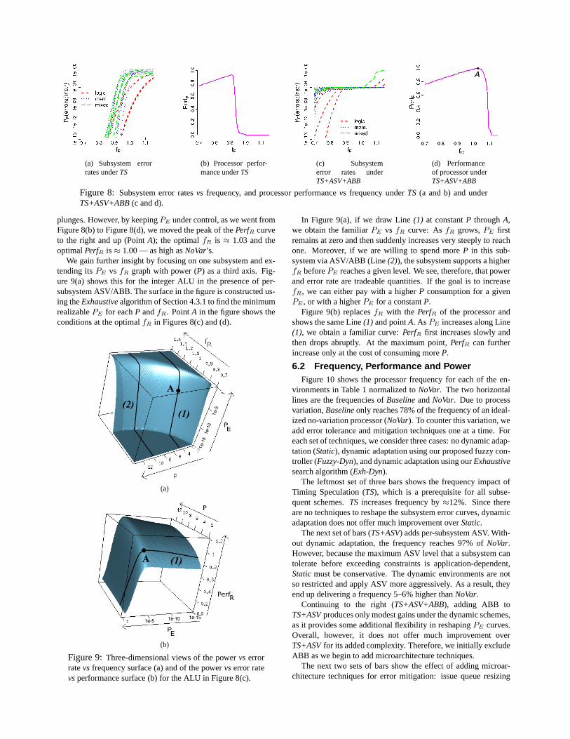
In our processor,PE , power, andf (or performance) are trade-able quantities. To show it, we experiment with one application(swim) running on one sample chip. For theTSenvironment, Fig-ure 8(a) shows thePE vs frequency curves of all the processor’ssubsystems. ThePE curves are labeled based on the type of sub-system (logic, memory, or mixed), while the frequency (fR) isshown relative to theNoVarenvironment (Table 1). In the figure,the slope of thePE curves depends primarily on the subsystemtype. Memory subsystems, with their homogeneous paths, have arapid error onset. Logic subsystems have a wide variety of pathsand, therefore, produce a more gradual error onset. Mixed sub-systems fall between the two extremes.

Figure 8(b) shows the processor performance relative toNoVar(PerfR) as a function of frequency. As indicated in Section 3.1, asfrequency increases, performance improves as long asPE (Fig-ure 8(a)) is not prohibitively high. AsPE increases past a criticalpoint,PerfR falls off sharply. From Figure 8(b), we see that, withTS, the processor runs optimally atfR ≈ 0.91 (that is, slowerthanNoVar) and delivers aPerfR ≈ 0.92 (again, lower thanNo-Var). This is much better than underBaseline, which cannot tol-erate any error. Indeed,Baselinecan only run at thefR wherethe leftmostPE curve in Figure 8(a) intersects thex-axis (fR ≈0.84).

To improvePerfR, we need to delay the exponentialPE onset.To this end, Figures 8(c) and (d) repeat thePE andPerfR curvesfor an environment that has per-subsystem ASV and ABB — setby theExhaustivealgorithm of Section 4.3.1. For eachfR, thisalgorithm finds a configuration where the sum of allPE curvesis ≈ 10−4 errs/inst, which isPEMAX . This is accomplished byspeeding up slow subsystems and saving power on fast ones. Thisis why Figure 8(c) shows a convergence of lines atPE ≈ 10−4.However, for highfR, it becomes increasingly power-costly tokeepPE ≤ PEMAX . Eventually, the power constraint is reached,and no further ASV/ABB can be applied to speed up subsystemsand keepPE ≤ PEMAX . Then, as can be seen in Figure 8(c),somePE curves escape up and, as shown in Figure 8(d),PerfR

(a) Subsystem errorrates underTS

(b) Processor perfor-mance underTS

(c) Subsystemerror rates underTS+ASV+ABB

A

(d) Performanceof processor underTS+ASV+ABB

Figure 8: Subsystem error ratesvs frequency, and processor performancevs frequency underTS (a and b) and underTS+ASV+ABB(c and d).

plunges. However, by keepingPE under control, as we went fromFigure 8(b) to Figure 8(d), we moved the peak of thePerfR curveto the right and up (PointA); the optimalfR is ≈ 1.03 and theoptimalPerfR is≈ 1.00 — as high asNoVar’s.

We gain further insight by focusing on one subsystem and ex-tending itsPE vs fR graph with power (P) as a third axis. Fig-ure 9(a) shows this for the integer ALU in the presence of per-subsystem ASV/ABB. The surface in the figure is constructed us-ing theExhaustivealgorithm of Section 4.3.1 to find the minimumrealizablePE for eachP andfR. PointA in the figure shows theconditions at the optimalfR in Figures 8(c) and (d).

(a)

(b)

Figure 9:Three-dimensional views of the powervserrorratevs frequency surface (a) and of the powervserror ratevsperformance surface (b) for the ALU in Figure 8(c).

In Figure 9(a), if we draw Line(1) at constantP throughA,we obtain the familiarPE vs fR curve: AsfR grows,PE firstremains at zero and then suddenly increases very steeply to reachone. Moreover, if we are willing to spend moreP in this sub-system via ASV/ABB (Line(2)), the subsystem supports a higherfR beforePE reaches a given level. We see, therefore, that powerand error rate are tradeable quantities. If the goal is to increasefR, we can either pay with a higherP consumption for a givenPE , or with a higherPE for a constantP.

Figure 9(b) replacesfR with the PerfR of the processor andshows the same Line(1) and pointA. AsPE increases along Line(1), we obtain a familiar curve:PerfR first increases slowly andthen drops abruptly. At the maximum point,PerfR can furtherincrease only at the cost of consuming moreP.

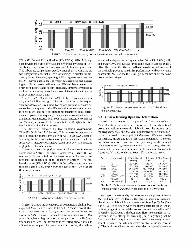
6.2 Frequency, Performance and PowerFigure 10 shows the processor frequency for each of the en-

vironments in Table 1 normalized toNoVar. The two horizontallines are the frequencies ofBaselineandNoVar. Due to processvariation,Baselineonly reaches 78% of the frequency of an ideal-ized no-variation processor (NoVar). To counter this variation, weadd error tolerance and mitigation techniques one at a time. Foreach set of techniques, we consider three cases: no dynamic adap-tation (Static), dynamic adaptation using our proposed fuzzy con-troller (Fuzzy-Dyn), and dynamic adaptation using ourExhaustivesearch algorithm (Exh-Dyn).

The leftmost set of three bars shows the frequency impact ofTiming Speculation (TS), which is a prerequisite for all subse-quent schemes.TS increases frequency by≈12%. Since thereare no techniques to reshape the subsystem error curves, dynamicadaptation does not offer much improvement overStatic.

The next set of bars (TS+ASV) adds per-subsystem ASV. With-out dynamic adaptation, the frequency reaches 97% ofNoVar.However, because the maximum ASV level that a subsystem cantolerate before exceeding constraints is application-dependent,Staticmust be conservative. The dynamic environments are notso restricted and apply ASV more aggressively. As a result, theyend up delivering a frequency 5–6% higher thanNoVar.

Continuing to the right (TS+ASV+ABB), adding ABB toTS+ASVproduces only modest gains under the dynamic schemes,as it provides some additional flexibility in reshapingPE curves.Overall, however, it does not offer much improvement overTS+ASVfor its added complexity. Therefore, we initially excludeABB as we begin to add microarchitecture techniques.

The next two sets of bars show the effect of adding microar-chitecture techniques for error mitigation: issue queue resizing

TS TS+ASV TS+ASV+ABB TS+ASV+Q TS+ASV+Q+FU ALL

Re

lative

Fre

qu

en

cy

0.0

0.4

0.8

1.2

Baseline

Static Fuzzy!Dyn Exh!Dyn

NoVar

Figure 10:Processor frequency for each environment normalized toNoVar.

(TS+ASV+Q) and FU replication (TS+ASV+Q+FU). Althoughnot shown in the figure, if we add them without any ABB or ASVcapability, they deliver a disappointing 2% frequency increase.This is because temperatures stay low enough that optimizing thetwo subsystems does not deliver, on average, a substantial fre-quency boost. However, applying ASV to aggressively re-shapethe PE curves pushes the subsystem temperatures and powershigher. Under these conditions, the FUs and issue queues rou-tinely form hotspots and become frequency-limiters. By speedingup these critical subsystems, the microarchitectural techniques de-liver good frequency gains.

The TS+ASV+Q and TS+ASV+Q+FU environments showthat, to take full advantage of the microarchitecture techniques,dynamic adaptation is required. Not all applications or phases ex-ercise the issue queue or the FUs enough to make them critical.In these cases, statically enabling these techniques costs perfor-mance or power. Consequently, it makes sense to enable these op-timizations dynamically. With both microarchitecture techniquesandFuzzy-Dyn, we reach a frequency that is 21% higher thanNo-Var (or 56% higher thanBaseline).

The difference between the two rightmost environmentsTS+ASV+Q+FUandALL is small. This suggests that it is reason-able to forgo the added complexity of ABB in an EVAL system.Similarly, the difference between using a fuzzy adaptation scheme(Fuzzy-Dyn) instead of exhaustive search (Exh-Dyn) is practicallynegligible in all environments.

Figure 11 shows the performance of all these environmentsnormalized toNoVar. The figure is organized as Figure 10. Wesee that performance follows the same trends as frequency, ex-cept that the magnitude of the changes is smaller. The pre-ferred scheme (TS+ASV+Q+FUwith Fuzzy-Dyn) realizes a per-formance gain of 14% overNoVaror, equivalently, 40% over theBaselineprocessor.

TS TS+ASV TS+ASV+ABB TS+ASV+Q TS+ASV+Q+FU ALL

Re

lative

Pe

rfo

rma

nce

0.0

0.4

0.8

1.2

Baseline

Static Fuzzy!Dyn Exh!Dyn

NoVar

Figure 11:Performance of different environments.

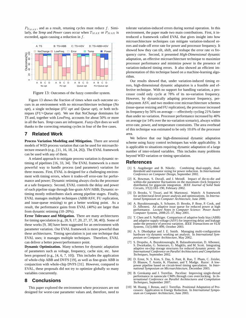
Figure 12 shows the average power consumed, including bothPdyn andPsta, in a core and its L1 and L2 caches. Recall that,for each processor, we setPMAX to 30W. We see that the averagepower forNoVar is 25W — although some processors reach 30Wat certain points of high activity and temperature — whileBase-line consumes 17W. The latter runs at lower frequency. As we addmitigation techniques, the power tends to increase, although its

actual value depends on many variables. WithTS+ASV+Q+FUand Fuzzy-Dyn, the average processor power is almost exactly30W. This shows that theFuzzy-Dyncontroller is making use ofthe available power to maximize performance without violatingconstraints. We also see thatExh-Dynconsumes about the samepower asFuzzy-Dyn.

TS TS+ASV TS+ASV+ABB TS+ASV+Q TS+ASV+Q+FU ALL

Pow

er (

W)

010

2030

Baseline

NoVar

Static Fuzzy−Dyn Exh−Dyn

Figure 12:Power per processor (core+L1+L2) for differ-ent environments.

6.3 Characterizing Dynamic AdaptationFinally, we compare the output of the fuzzy controller to

Exhaustiveto show why fuzzy control provides nearly optimalpower and performance results. Table 2 shows the mean error inthe frequency,Vdd, andVbb values generated by the fuzzy con-troller compared to the output ofExhaustive. We show resultsfor memory, mixed, and logic subsystems separately. The errorsare shown in absolute units and as a percentage of the nominalvalue (except forVbb, where the nominal value is zero). The tableshows that, in practically all cases, the fuzzy controller predictsfrequency,Vdd and, to a lesser extent,Vbb, quite accurately.

Param. Environment | Fuzzy Controller - Exhaustive| (% of Nom.)Memory Mixed Logic

TS 168 (4.1%) 146 (3.6%) 170 (4.2%)Freq. TS+ABB 170 (4.2%) 135 (3.3%) 149 (3.6%)(MHz) TS+ASV 450 (11.0%) 410 (10.0%) 160 (3.9%)

TS+ABB+ASV 176 (4.3%) 162 (4.0%) 146 (3.6%)Vdd TS+ASV 17 (1.7%) 24 (2.4%) 14 (1.4%)(mV) TS+ABB+ASV 16 (1.6%) 22 (2.2%) 22 (2.2%)Vbb TS+ABB 72 (–) 69 (–) 76 (–)(mV) TS+ABB+ASV 115 (–) 129 (–) 124 (–)

Table 2: Difference between the selections of the fuzzycontroller andExhaustivein absolute and relative terms.

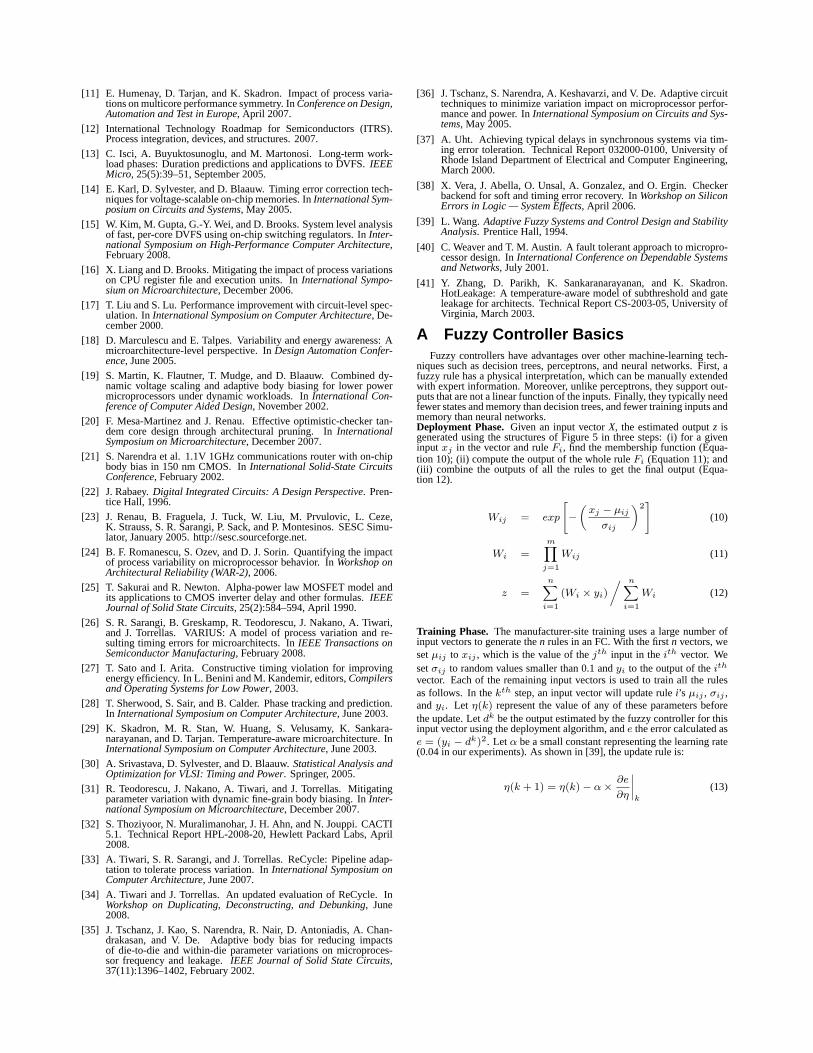
An important reason why the performance and power ofFuzzy-Dyn and Exh-Dyn are largely the same despite any inaccura-cies shown in Table 2 is the presence ofRetuning Cycles(Sec-tion 4.3.3). Specifically, when the fuzzy controller algorithm se-lects a configuration, any of the five outcomes shown in Figure 13is possible.NoChangeis the best case. Here, no constraint is vio-lated and the first attempt at increasingf fails, signifying that thefuzzy controller’s output was near optimal. InLowFreq, no con-straint is violated, but retuning cycles are able to further increasef . The third case (Error) occurs when the configuration violates

PEMAX , and as a result, retuning cycles must reducef . Simi-larly, theTempandPowercases occur whenTMAX or PMAX isexceeded, again causing a reduction inf .

A B C D A B C D A B C D A B C D

Out

com

es(%

)0

2040

6080

100

No opt FU opt Queue opt FU+Queue opt

NoChange LowFreq. Error Temp Power

A: TS B: TS+ABB C: TS+ASV D: TS+ABB+ASV

Figure 13:Outcomes of the fuzzy controller system.

Figure 13 shows the fraction of times when each outcome oc-curs in an environment with no microarchitecture technique (Noopt), a single technique (FU opt andQueue opt), or both tech-niques (FU+Queue opt). We see thatNoChangedominates forTSand, together withLowFreq, accounts for about 50% or morein all the bars.Tempcases are infrequent.Fuzzy-Dyndoes so wellthanks to the correcting retuning cycles in four of the five cases.

7 Related WorkProcess Variation Modeling and Mitigation. There are severalmodels of WID process variation that can be used for microarchi-tecture research (e.g., [11, 16, 18, 24, 26]). The EVAL frameworkcan be used with any of them.

A related approach to mitigate process variation is dynamic re-timing of pipelines [16, 33, 34]. The EVAL framework is a morepowerful way to handle process (and parameter) variation forthree reasons. First, EVAL is designed for a challenging environ-ment with timing errors, where it trades-off error-rate for perfor-mance and power; Dynamic retiming always clocks the processorat a safe frequency. Second, EVAL controls the delay and powerof each pipeline stage through fine-grain ASV/ABB; Dynamic re-timing mostly redistributes slack among pipeline stages. Finally,EVAL manages multiple techniques (ABB/ASV, FU replication,and issue-queue resizing) to get a better working point. As aresult, the performance gains from EVAL (40%) are larger thanfrom dynamic retiming (10–20%).Error Tolerance and Mitigation. There are many architecturesfor timing speculation (e.g., [8, 9, 17, 20, 27, 37, 38, 40]). Some ofthese works [9, 38] have been suggested for an environment withparameter variation. Our EVAL framework is more powerful thanthese architectures. Timing speculation is just one technique thatEVAL uses; it manages multiple techniques. Therefore, EVALcan deliver a better power/performance point.Dynamic Optimization. Many schemes for dynamic adaptationof parameters such as voltage, frequency, cache size, etc. havebeen proposed (e.g., [4, 6, 7, 10]). This includes the applicationof whole-chip ABB and DVFS [19], as well as fine-grain ABB inconjunction with whole-chip DVFS [31]. However, compared toEVAL, these proposals did not try to optimize globally so manyvariables concurrently.

8 ConclusionsThis paper explored the environment where processors are not

designed for worst-case parameter values and, therefore, need to

tolerate variation-induced errors during normal operation. In thisenvironment, the paper made two main contributions. First, it in-troduced a framework called EVAL that gives insight into howmicroarchitecture techniques can mitigate variation-induced er-rors and trade-off error rate for power and processor frequency. Itshowed how they can tilt, shift, and reshape the error ratevs fre-quency curve. Second, it presentedHigh-Dimensionaldynamicadaptation, an effective microarchitecture technique to maximizeprocessor performance and minimize power in the presence ofvariation-induced timing errors. It also showed an efficient im-plementation of this technique based on a machine-learning algo-rithm.

Our results showed that, under variation-induced timing er-rors, high-dimensional dynamic adaptation is a feasible and ef-fective technique. With no support for handling variation, a pro-cessor could only cycle at 78% of its no-variation frequency.However, by dynamically adapting processor frequency, per-subsystem ASV, and two modest-cost microarchitecture schemes(issue-queue resizing and FU replication), the processor increasedits frequency by 56% on average — effectively cycling 21% fasterthan under no variation. Processor performance increased by 40%on average (or 14% over the no-variation scenario), always withinerror-rate, power, and temperature constraints. The area overheadof this technique was estimated to be only 10.6% of the processorarea.

We believe that our high-dimensional dynamic adaptationscheme using fuzzy control techniques has wide applicability. Itis applicable to situations requiring dynamic adaptation of a largenumber of inter-related variables. This includes many problemsbeyond WID variation or timing speculation.

References[1] S. Augsburger and B. Nikolic. Combining dual-supply, dual-

threshold and transistor sizing for power reduction. InInternationalConference on Computer Design, September 2002.

[2] K. Bowman, S. Duvall, and J. Meindl. Impact of die-to-die andwithin-die parameter fluctuations on the maximum clock frequencydistribution for gigascale integration.IEEE Journal of Solid StateCircuits, 37(2):183–190, February 2002.

[3] D. Brooks, V. Tiwari, and M. Martonosi. Wattch: A frameworkfor architectural-level power analysis and optimizations. InInterna-tional Symposium on Computer Architecture, June 2000.

[4] A. Buyuktosunoglu, S. Schuster, D. Brooks, P. Bose, P. Cook, andD. Albonesi. An adaptive issue queue for reduced power at highperformance. Lecture Notes in Computer Science: Power AwareComputer Systems, 2008:25–37, May 2001.

[5] T. Chen and S. Naffziger. Comparison of adaptive body bias (ABB)and adaptive supply voltage (ASV) for improving delay and leakageunder the presence of process variation.IEEE Transactions on VLSISystems, 11(5):888–899, October 2003.

[6] A. S. Dhodapkar and J. E. Smith. Managing multi-configurationhardware via dynamic working set analysis. InInternational Sym-posium on Computer Architecture, May 2002.

[7] S. Dropsho, A. Buyuktosunoglu, R. Balasubramonian, D. Albonesi,S. Dwarkadas, G. Semeraro, G. Magklis, and M. Scott. Integratingadaptive on-chip storage structures for reduced dynamic power. InInternational Conference on Parallel Architectures and CompilationTechniques, September 2002.

[8] D. Ernst, N. S. Kim, S. Das, S. Pant, R. Rao, T. Pham, C. Zeisler,D. Blaauw, T. Austin, K. Flautner, and T. Mudge. Razor: A low-power pipeline based on circuit-level timing speculation. InInter-national Symposium on Microarchitecture, December 2003.

[9] B. Greskamp and J. Torrellas. Paceline: Improving single-threadperformance in nanoscale CMPs through core overclocking. InIn-ternational Conference on Parallel Architectures and CompilationTechniques, September 2007.

[10] M. Huang, J. Renau, and J. Torrellas. Positional Adaptation of Pro-cessors: Application to Energy Reduction. InInternational Sympo-sium on Computer Architecture, June 2003.

[11] E. Humenay, D. Tarjan, and K. Skadron. Impact of process varia-tions on multicore performance symmetry. InConference on Design,Automation and Test in Europe, April 2007.

[12] International Technology Roadmap for Semiconductors (ITRS).Process integration, devices, and structures. 2007.

[13] C. Isci, A. Buyuktosunoglu, and M. Martonosi. Long-term work-load phases: Duration predictions and applications to DVFS.IEEEMicro, 25(5):39–51, September 2005.

[14] E. Karl, D. Sylvester, and D. Blaauw. Timing error correction tech-niques for voltage-scalable on-chip memories. InInternational Sym-posium on Circuits and Systems, May 2005.

[15] W. Kim, M. Gupta, G.-Y. Wei, and D. Brooks. System level analysisof fast, per-core DVFS using on-chip switching regulators. InInter-national Symposium on High-Performance Computer Architecture,February 2008.

[16] X. Liang and D. Brooks. Mitigating the impact of process variationson CPU register file and execution units. InInternational Sympo-sium on Microarchitecture, December 2006.

[17] T. Liu and S. Lu. Performance improvement with circuit-level spec-ulation. InInternational Symposium on Computer Architecture, De-cember 2000.

[18] D. Marculescu and E. Talpes. Variability and energy awareness: Amicroarchitecture-level perspective. InDesign Automation Confer-ence, June 2005.

[19] S. Martin, K. Flautner, T. Mudge, and D. Blaauw. Combined dy-namic voltage scaling and adaptive body biasing for lower powermicroprocessors under dynamic workloads. InInternational Con-ference of Computer Aided Design, November 2002.

[20] F. Mesa-Martinez and J. Renau. Effective optimistic-checker tan-dem core design through architectural pruning. InInternationalSymposium on Microarchitecture, December 2007.

[21] S. Narendra et al. 1.1V 1GHz communications router with on-chipbody bias in 150 nm CMOS. InInternational Solid-State CircuitsConference, February 2002.

[22] J. Rabaey.Digital Integrated Circuits: A Design Perspective. Pren-tice Hall, 1996.

[23] J. Renau, B. Fraguela, J. Tuck, W. Liu, M. Prvulovic, L. Ceze,K. Strauss, S. R. Sarangi, P. Sack, and P. Montesinos. SESC Simu-lator, January 2005. http://sesc.sourceforge.net.

[24] B. F. Romanescu, S. Ozev, and D. J. Sorin. Quantifying the impactof process variability on microprocessor behavior. InWorkshop onArchitectural Reliability (WAR-2), 2006.

[25] T. Sakurai and R. Newton. Alpha-power law MOSFET model andits applications to CMOS inverter delay and other formulas.IEEEJournal of Solid State Circuits, 25(2):584–594, April 1990.

[26] S. R. Sarangi, B. Greskamp, R. Teodorescu, J. Nakano, A. Tiwari,and J. Torrellas. VARIUS: A model of process variation and re-sulting timing errors for microarchitects. InIEEE Transactions onSemiconductor Manufacturing, February 2008.

[27] T. Sato and I. Arita. Constructive timing violation for improvingenergy efficiency. In L. Benini and M. Kandemir, editors,Compilersand Operating Systems for Low Power, 2003.

[28] T. Sherwood, S. Sair, and B. Calder. Phase tracking and prediction.In International Symposium on Computer Architecture, June 2003.

[29] K. Skadron, M. R. Stan, W. Huang, S. Velusamy, K. Sankara-narayanan, and D. Tarjan. Temperature-aware microarchitecture. InInternational Symposium on Computer Architecture, June 2003.

[30] A. Srivastava, D. Sylvester, and D. Blaauw.Statistical Analysis andOptimization for VLSI: Timing and Power. Springer, 2005.

[31] R. Teodorescu, J. Nakano, A. Tiwari, and J. Torrellas. Mitigatingparameter variation with dynamic fine-grain body biasing. InInter-national Symposium on Microarchitecture, December 2007.

[32] S. Thoziyoor, N. Muralimanohar, J. H. Ahn, and N. Jouppi. CACTI5.1. Technical Report HPL-2008-20, Hewlett Packard Labs, April2008.

[33] A. Tiwari, S. R. Sarangi, and J. Torrellas. ReCycle: Pipeline adap-tation to tolerate process variation. InInternational Symposium onComputer Architecture, June 2007.

[34] A. Tiwari and J. Torrellas. An updated evaluation of ReCycle. InWorkshop on Duplicating, Deconstructing, and Debunking, June2008.

[35] J. Tschanz, J. Kao, S. Narendra, R. Nair, D. Antoniadis, A. Chan-drakasan, and V. De. Adaptive body bias for reducing impactsof die-to-die and within-die parameter variations on microproces-sor frequency and leakage.IEEE Journal of Solid State Circuits,37(11):1396–1402, February 2002.

[36] J. Tschanz, S. Narendra, A. Keshavarzi, and V. De. Adaptive circuittechniques to minimize variation impact on microprocessor perfor-mance and power. InInternational Symposium on Circuits and Sys-tems, May 2005.

[37] A. Uht. Achieving typical delays in synchronous systems via tim-ing error toleration. Technical Report 032000-0100, University ofRhode Island Department of Electrical and Computer Engineering,March 2000.

[38] X. Vera, J. Abella, O. Unsal, A. Gonzalez, and O. Ergin. Checkerbackend for soft and timing error recovery. InWorkshop on SiliconErrors in Logic — System Effects, April 2006.

[39] L. Wang.Adaptive Fuzzy Systems and Control Design and StabilityAnalysis. Prentice Hall, 1994.

[40] C. Weaver and T. M. Austin. A fault tolerant approach to micropro-cessor design. InInternational Conference on Dependable Systemsand Networks, July 2001.

[41] Y. Zhang, D. Parikh, K. Sankaranarayanan, and K. Skadron.HotLeakage: A temperature-aware model of subthreshold and gateleakage for architects. Technical Report CS-2003-05, University ofVirginia, March 2003.

A Fuzzy Controller BasicsFuzzy controllers have advantages over other machine-learning tech-

niques such as decision trees, perceptrons, and neural networks. First, afuzzy rule has a physical interpretation, which can be manually extendedwith expert information. Moreover, unlike perceptrons, they support out-puts that are not a linear function of the inputs. Finally, they typically needfewer states and memory than decision trees, and fewer training inputs andmemory than neural networks.Deployment Phase.Given an input vectorX, the estimated outputz isgenerated using the structures of Figure 5 in three steps: (i) for a giveninput xj in the vector and ruleFi, find the membership function (Equa-tion 10); (ii) compute the output of the whole ruleFi (Equation 11); and(iii) combine the outputs of all the rules to get the final output (Equa-tion 12).

Wij = exp

[−

(xj − µij

σij

)2]

(10)

Wi =m∏

j=1

Wij (11)

z =

n∑i=1

(Wi × yi)

/ n∑i=1

Wi (12)

Training Phase. The manufacturer-site training uses a large number ofinput vectors to generate then rules in an FC. With the firstn vectors, wesetµij to xij , which is the value of thejth input in theith vector. Wesetσij to random values smaller than 0.1 andyi to the output of theith

vector. Each of the remaining input vectors is used to train all the rulesas follows. In thekth step, an input vector will update rulei’s µij , σij ,andyi. Let η(k) represent the value of any of these parameters beforethe update. Letdk be the output estimated by the fuzzy controller for thisinput vector using the deployment algorithm, ande the error calculated ase = (yi − dk)2. Let α be a small constant representing the learning rate(0.04 in our experiments). As shown in [39], the update rule is:

η(k + 1) = η(k)− α×∂e

∂η

∣∣∣∣k

(13)