Estimation of Transport-Category Jet Airplane Maximum ...

Citation: Wislicenus, J.; Daidzic, N.E.

Estimation of Transport-Category Jet

Airplane Maximum Range and

Airspeed in the Presence of Transonic

Wave Drag. Aerospace 2022, 9, 192.

https://doi.org/10.3390/

aerospace9040192

Academic Editor: Kojiro Suzuki

Received: 19 October 2021

Accepted: 23 March 2022

Published: 2 April 2022

Publisher’s Note: MDPI stays neutral

with regard to jurisdictional claims in

published maps and institutional affil-

iations.

Copyright: © 2022 by the authors.

Licensee MDPI, Basel, Switzerland.

This article is an open access article

distributed under the terms and

conditions of the Creative Commons

Attribution (CC BY) license (https://

creativecommons.org/licenses/by/

4.0/).

aerospace

Article

Estimation of Transport-Category Jet Airplane Maximum Rangeand Airspeed in the Presence of Transonic Wave DragJan Wislicenus 1 and Nihad E. Daidzic 2,3,*

1 Department of Aerospace and Geodesy, Technical University of Munich, 80333 Munich, Germany;[email protected]

2 Department of Aviation, Minnesota State University, Mankato, MN 56001, USA3 AAR Aerospace Consulting, LLC, Saint Peter, MN 56082, USA* Correspondence: [email protected]

Abstract: One of the most difficult steps in estimating the cruise performance characteristics ofhigh-subsonic transport-category turbofan-powered airplanes is the estimation of the transonic wavedrag. Modern jet airplanes cruise most efficiently in the vicinity of the drag-divergence or drag-riseMach numbers. In the initial design phase and later when the preliminary wind-tunnel and/orCFD computations and drag polars are known with increased accuracy, a method of estimatingcruise performance is needed. In this study, a new semi-empirical transonic wave drag model usingmodified Lock’s equation was developed. For maximum range cruise estimations, an optimizationcriterion based on maximizing specific air range was used. The resulting nonlinear equations are of12th- and 13th-order. Numerical Newton–Raphson nonlinear solvers were used to find real positiveroots of such polynomials. The NR method was first tested for accuracy and convergence usingknown analytical solutions. A methodology for an initial guess was developed starting with themaximum-range cruise Mach without the wave-drag included. This guess resulted in fast quadraticconvergence in all computations. Other novel features of this article include a new semi-empiricalfuel-flow law, which was also extensively tested. Additionally, a semi-empirical turbofan thrustmodel usable for a wide range of bypass ratios and the entire flight envelope was developed. Suchphysics-based semi-empirical model can be used for a wide range of turbofans. The algorithm canbe utilized to identify most beneficial input parameter values and combinations for the cruise flightphase. The model represents a powerful tool to estimate important cruise performance airspeedslocated in the transonic regime. An intended application is in the conceptual development stages forearly design optimizations of future airplanes. It is possible with additional effort to extend existingmodel capabilities to deal with supersonic transports optimal cruise parameters.

Keywords: transonic wave drag; maximum range cruise; performance airspeeds; nonlinear equationssolvers; convergence of the Newton–Raphson method

1. Introduction

Estimation of performance airspeeds for various phases of high-subsonic transport-category (T-category) airplanes is an essential element in aircraft design, flight testing,certification, and in-service line operations. If the manufacturer’s advertised cruise speci-fications in terms of airspeeds, ranges, and endurances are not met, it could render newaircraft designs obsolete and unattractive and result in costly redesigns and delays. Thisapplies today to high-subsonic designs, but it is equally and perhaps even more criticalfor the future supersonic, hypersonic, and spaceplane designs. Performing transonic CFDand utilizing high-speed wind tunnels for proof of concept and actual designs is expensiveand time consuming. In the end, what sells aerospace transports is not utilization of com-plex CFD or transonic wind tunnels but ultimately meeting the advertised performancecharacteristics in operational service.

Aerospace 2022, 9, 192. https://doi.org/10.3390/aerospace9040192 https://www.mdpi.com/journal/aerospace

https://doi.org/10.3390/aerospace9040192


https://creativecommons.org/

https://creativecommons.org/licenses/by/4.0/

https://creativecommons.org/licenses/by/4.0/

https://www.mdpi.com/journal/aerospace

https://www.mdpi.com

https://orcid.org/0000-0003-0193-1328

https://orcid.org/0000-0001-6262-110X


https://www.mdpi.com/journal/aerospace

https://www.mdpi.com/article/10.3390/aerospace9040192?type=check_update&version=1

Aerospace 2022, 9, 192 2 of 28

For modern high-subsonic cruisers, the estimation of the transonic wave drag, andcomputation of cruise performance characteristic is essential. Having a performance toolthat integrates airplane components and airframe and powerplants characteristics anddelivers essential performance figures is essential. Obtaining drag polars from the initialwind-tunnel testing and/or CFD efforts also allows for analytical/numerical treatmentof performance airspeeds. No matter how effective CFD computations are at deliveringpressure, temperature, and velocity distributions, the spatial results need to be integratedand presented in terms of aerodynamic coefficients for the entire aircraft so that perfor-mance analysis can be completed. In the first design estimates, drag polars and otheraerodynamic and powerplant characteristics are not fully known, and this is an iterativeprocess that hopefully converges toward desired evolutionary designs. Flight testing ofprototypes will deliver final aerodynamic and propulsion characteristics that can be thenfed to performance calculators to deliver in-service figures and can be also used for crewtraining and development of the best operational practices.

Unrealistic cruise ranges and airspeeds are obtained if the transonic wave drag isnot properly accounted for in the high-speed cruise performance computations for high-subsonic T-category jet airplanes. While accounting for only few percentages of the totaldrag, the transonic wave-drag is concentrated in that high-speed range and has an essentialeffect on high-speed parameters. The transonic wave-drag differs from the supersonicwave-drag, mostly due to shock formation over the upper and lower wing surfaces andtheir interference with the boundary layer (BL). Often due to adverse pressure gradientsacross the shock, thickening and possible separation of the BL occurs, resulting in additionaltransonic pressure-drag. Supersonic wave drag is mostly the result of the kinetic energyloss through the bow and rear shocks. Total drag rise in transonic flow becomes especiallytroublesome as Mach-rise or Mach drag-divergence (MDD) is exceeded. While wing sweepwill increase freestream critical Mach number (MCR) and delay the onset of shocks, it is thesupercritical wing design that will expand the range between the MCR and MDD. In termsof range and economy of flight, it is normally not efficient to fly faster than MDD as thedrag increase may become very steep, thus reducing the maximum range.

Most of the modern high-subsonic swept-wing T-category jet airplanes certified un-der FAA FAR 25 (USA), EASA CS 25 (EU), etc., worldwide operate at Mach numbersexceeding critical Mach numbers by small amounts, thus ensuring locally transonic flows.The transonic region is defined for the range of freestream supercritical Mach numbers,typically between 0.75 and 1.2, but that classification is somewhat arbitrary and airplane-design dependent. Transonic flow regime consists of pockets of subsonic and supersonicflows. Lower regions of boundary layers are subsonic, while the outer parts may becomesupersonic.

Before we proceed, we must underscore that the approach adopted here is an integralmodelling of the transonic wave-drag in terms of a complex nonlinear algebraic modeland not in any kind of CFD computations or experimental results. The algebraic model oftotal airplane drag includes somewhat novel transonic wave-drag module based on themodified Lock’s integral momentum equation for speeds slightly above the critical Machnumbers and only on the subsonic side. In doing so, we also incorporated algebraic modelsfor turbofan engines and fuel flow laws, which enabled treatment of optimal performancecruise airspeeds based on one optimization criteria (maximizing still-air ranges). Hence, thisarticle does not go into any specific detail of complex transonic flow phenomena simulatingshocks and detailed flow parameters (such as air speed and pressure distributions) overmodern supercritical wings, other than giving a brief description of the problem andbasic equations, but instead focuses on high-subsonic cruise performance optimization,which is of ultimate operational significance. Naturally, the model developed here isbased on several assumptions regarding various drag components that must be checkedcomputationally, experimentally, and ultimately during certification flight tests. Results interms of airspeeds and ranges were compared to real high-subsonic airplane performance,and very reasonable estimates were obtained.

Aerospace 2022, 9, 192 3 of 28

Detailed treatment of transonic flow over aircraft structures accounting for variousinteractions is one of the most challenging problems in the aerodynamics of compressibleflows. Specialized high-speed wind tunnels and transonic CFD computations are theprimary tools in treating transonic flows. Shock-wave/boundary-layer interactions (SWBLI)with their intricacies are also fundamental in transonic flow computations. Computationally,transonic flow problems can be treated, in the order of complexity and difficulty, as:

• Small-perturbation potential-flow transonic flow equation.• Full nonlinear potential equation for inviscid, isentropic, and irrotational flow assum-

ing weak (third-order entropy increase) shocks.• Euler equations for adiabatic inviscid but rotational flows.• RANS-LES-DES simulations using Reynolds-averaged Navier–Stokes equations with

various turbulence modelling methods and models.• DNS simulations using spatially and temporally discretized Navier–Stokes equations.

Significant progress has been achieved in computational compressible aerodynamicsand CFD utilization in aircraft design over the past 50 years. Enlightening historicalreviews of existing state of the art computational aerodynamics and aircraft CFD designprogress and developments are given by [1–4]. Important references dealing specificallywith transonic flow and wave drag computations are given in [5–8]. A discussion ofcomputational capabilities utilizing RANS/LES transonic flow predictions was publishedin a recent review of RANS/LES turbulent flow modelling by [9].

SWBLIs play fundamental role in transonic wave drag physics due to thickening ofthe boundary layers (increasing profile drag) and possibly causing separation of the BL,which may result in shock-stall or high-speed buffet. Much has been published on SWBLI,and more or less detailed considerations can be found, for example, in [10–12]. A goodintroduction to SWBLI with laminar and turbulent BLs is also given in [13]. The detailedphysics of shock waves was examined in the classical works by [14] and in particular in [15].Inviscid hypersonic flow was examined in depth in [16]. Detailed consideration of bothinviscid and viscous hypersonic flight is given, for example, in [17].

An early treasure in analysis of subsonic, transonic, and supersonic airplane flightpaths from spherical rotating to simple flat non-rotating Earth is a book by Miele [18].Parabolic and arbitrary drag polars were used in addition to some simple fuel laws andengine characteristics. Many different cases were considered, including early consider-ations of optimal level cruise. Superb treatment of subsonic, transonic, and supersonicaerodynamics with many important details is given in Küechemann [19]. The author’streatment of swept wings in transonic (and supersonic) flight is especially important forus. Shevell [20] introduces the compressibility effects and drag on airfoils and wings. Theauthor also provides a semi-empirical relationship for the estimation of drag-divergenceMach number based on the critical Mach number for swept wings. Menon [21] has studiedaircraft cruise from the aspect of trajectory optimization and compared his theory with thepoint-mass and energy models. The author has shown that oscillatory cruise trajectoriesexist if the Hessian of a characteristic function is positive definite. Miller [22] also studiedoptimal cruise performance and the determination of optimal cruise speeds. Miller hasconcluded that the optimal cruise Mach number occurs in the drag-rise (transonic) region,i.e., between MCR and MDD. Wave drag becomes noticeable once MCR is exceeded but trulysignificant once MDD is surpassed. Mason [5] uses potential flow model for aerodynamic de-sign at transonic speeds. The author points out principal shortcomings of the potential flowmodels in terms that can be easily understood by aerodynamicists. Malone and Mason [23]present an approach to multidisciplinary aircraft design optimization that combines globalsensitivity equation method, parametric optimization, and analytic technology models.An expression for wave-drag and MDD is given for swept-wing aircraft—an extensionof the classical Korn equation. Torenbeek [24] provides very exhaustive consideration, aunified analytical treatment, and optimization techniques for the cruise performance ofsubsonic transport aircraft. A simple alternative to the celebrated Bréguet range equationis presented that applies to several practical cruise techniques. A practical non-iterative

Aerospace 2022, 9, 192 4 of 28

procedure for computing mission fuel and reserve fuel loads in the preliminary designstage is proposed. Mason [25] provides extended summary of transonic aerodynamicsof airfoils and (finite) wings. The historical development and facts were included thatshow the tortuous path that must be traveled to understand and solve transonic flowproblems. All operating considerations are based on the cost index (CI), which is themost suitable method in defining the new economical long-range cruise (ELRC). Fujinoand Kawamura [6] present an experimental and theoretical study of wave-drag reductionand increase in MDD in the case of over-the-wing nacelle configuration. Such nacelleconfiguration reduces transonic cruise drag without altering the original geometry of thenatural-laminar-flow wing. Jakirlic et al. [26] implemented CFD for performance estimationof supercritical transonic RAE2822 airfoil profiles. A near-wall RANS viscous turbulencemodel was used. Very recently, Friedewald [27] used URANS simulations for sinusoidalgust load modelling of often-used testbed RAE2822 airfoil involving different transonicMach numbers and using in-house-developed DLR TAU code based on a finite-volumeRANS solver.

Cavcar and Cavcar [28] delivered approximate cruise range solutions for the constant-altitude and constant high-subsonic cruise speed of transport category aircraft with cam-bered wing designs. The authors also used Mach-dependent specific fuel consumption(SFC), which differs from the one introduced in this work. The effect of Mach numberon the drag polar was evident when deriving approximate solutions. Wave drag wasconsidered when estimating optimum cruise factor. It was found that compressibilityeffects necessitate use of higher-order polynomial drag polar. Rivas and Valenzuela [29]analyzed maximum range cruise at constant altitude as a singular optimal control problemfor an aircraft model with a general compressible drag polar. Compressibility effects mustbe considered when seeking optimum cruise solutions in terms of speed and range. Theinfluence of flight altitude on optimal trajectories was shown to be important as well.Results presented were for a B767-300ER model, a popular long-range twin-jet design fromearly 1980’s. Daidzic [30] discussed global range of subsonic and supersonic airplanes andthe aerodynamic and propulsion developments needed.

A method to compute various performance airspeeds of FAR/CS 25 T-category turbo-fan airplanes was developed by Daidzic [31]. Newton–Raphson (NR) nonlinear-equationsolvers were used to find real positive zeros of high-order polynomials. However, theparabolic-drag model lacked (transonic) wave-drag, resulting in overestimation of maxi-mum airspeeds and unrealistic still-air ranges. Wave drag originates in the formation ofshock waves in supercritical subsonic flow. Hence, a semi-empirical wave-drag model,which was added to parabolic subcritical compressible drag model to capture transonicwave drag and compute high-speed range, was developed. To the best knowledge of theauthors, no such publicly available complete method has been introduced before. The eco-nomic and environmental importance of finding optimum cruising parameters under givenatmospheric conditions in air transportation should not be overlooked. In Daidzic [30], bothsubsonic and supersonic cruisers were compared in terms of passenger-miles (or passenger-km) per mass or weight unit of fuel and other economic factors. Increasing cruise economyalso reduces environmental pollution and has wider positive socio-economic impact.

The basic methodology presented here could perhaps be extended to emerging hyper-sonic suborbital and even orbital reentry transports. For example, Daidzic [32] discussesthe conceptual design and analysis of hypersonic RBCC SSTO spaceplane with glidingreentry for cost-effective LEO access. The article by Fusaro at al. [33] is focused on theanalysis and methodology of lowering direct operating cost of long-haul point-to-pointhypersonic transportation systems from 90% to about 70% utilizing liquid-hydrogen (LH2).Viola et al. [34] in a recent article provided technical insights into the aerodynamic charac-terization of a Mach-8 waverider hypersonic civil transport. While we specifically considermodern high-subsonic T-category airplanes in this article, the basic methodology could beextended for use in supersonic transports.

Aerospace 2022, 9, 192 5 of 28

Transonic flow problems, even in linearized form assuming small angles-of-attack(AOA) and thin airfoils, cannot be treated as easily as subcritical subsonic or fully developedsupersonic flows. This is because the small-perturbation potential transonic flow equationusing velocity potential for the inviscid irrotational flow remains nonlinear [35–39]:(

1−M2∞

)φxx + φyy + φzz = M2

∞

[(γ + 1)

φx

v∞

]· φxx (1)

This is a dramatically different situation from the linearized subcritical potentialflow equation, which is, de facto, linear and can be converted into the elliptic quasi-incompressible flow Laplace equation by proper coordinate transformation. Additionally,linearized small-perturbation subcritical potential flow results in the Prandtl–Glauertrule [35,36,39,40], which addresses the effect of shock-free air compressibility on the pres-sure, lift, and pitching-moment coefficients. Improved compressibility corrections wereobtained by Karman–Tsien [41,42] and Laitone [43] rules by considering local and notfreestream Mach numbers. Prandtl–Glauert compressibility correction diverges as Machone is approached and is not valid for transonic flow.

Inviscid irrotational CFD models can predict chordwise and spanwise pressure distri-butions and hence coefficients-of-lift and pitching-moments-coefficients with acceptableaccuracy. Full potential models include mass-, momentum-, and energy conservation inone single, albeit complex and nonlinear, velocity-potential PDE [35,36,39,40]:

(1− Φ2

xa2

)Φxx +

(1−

Φ2y

a2

)φyy +

(1− Φ2

za2

)Φzz −

2ΦxΦy

a2 Φxy −2ΦxΦz

a2 Φxz −2ΦyΦz

a2 Φyz = 0 (2)

where:a2 = a2

SL −γ− 1

2

(Φ2

x + Φ2y + Φ2

z

)(3)

The velocity vector is expressed by a scalar potential function for irrotational fieldeverywhere:

ς = curl v = ∇× v = ∇× (∇Φ) ≡ 0 ⇒ v = u→i + v

→j + w

→k = ∇Φ =

∂Φ∂x

→i +

∂Φ∂y

→j +

∂Φ∂z

→k (4)

Small perturbation or linearized (thin airfoils/wings and/or small AOAs) potentialequation with the Prandtl–Glauert compressibility-correction factor β for a swept wingwith sweep-angle Λ yields [13]:

β2φxx + φyy + φzz = 0 β =√

1−M2∞ cos2 Λ u′ =

∂φ

∂xv′ =

∂φ

∂yw′ =

∂φ

∂z(5)

This linear elliptic PDE, which is obtained from Equation (1) directly, is only valid forsubcritical subsonic range (M < MCR) and can be easily solved by coordinate transformationresulting in Laplace’s PDE [35,36,38]. The mixed supersonic-subsonic flow over transonicairfoils for two-dimensional geometry is treated by the hyperbolic-elliptic linear PDE orTricomi equation [36]. Supersonic linearized theory or Ackert’s rule (analog to subcriticalPrandtl–Glauert rule but on the supersonic side) is described, for example, in [13,35]. Thevalidity of asymptotic Ackert’s or Prandtl–Glauert rules ceases at the boundaries of thetransonic flow region, and small-perturbation transonic flow computations require use ofEquation (1).

Inviscid irrotational potential models can predict induced (vortex) drag and the wavedrag but cannot address the BL skin-friction drag and pressure drag due to BL separationand wakes. Inviscid full potential equation can be used for any inviscid irrotational flowfrom low subsonic to hypersonic. Panel methods could be used for subcritical compressibleflow on transformed Laplace equation but not for transonic flow. A good review ofpanel methods is given, for example, in [13,39]. An exceptional review of nonlinearpotential methods is given in [37]. Inviscid irrotational flow behind a curved shock-wave

Aerospace 2022, 9, 192 6 of 28

may become rotational, in which case Euler models, which do not require isentropic andirrotational conditions such as potential codes, are needed. Vorticity can exist in Euler’sinviscid flow, but the Euler equation itself provides no mechanisms for the generation(other than with curved shock waves) and dissipation of vorticity. Kelvin’s theorem ensuresthe conservation of circulation in such flows. However, continuity, three momentums forspeeds in each orthogonal direction, and the energy differential conservation equationsare required for this adiabatic, inviscid flow with no external body forces (gravity forceneglected), resulting in a system of five PDEs [35]:

∂ρ

∂t+∇ · (ρ v) = 0 ρ

D vDt

= −∇p ρD htot

D t=

∂p∂t

where htot ≡ hstatic +v2

2(6)

Using Lamb’s rotational form of the convective acceleration term in the material(substantial) derivative, one obtains the Euler equation with gravitational term neglected:

DvDt

=∂v∂t

+ (v · ∇)v =∂v∂t

+∇(

v2

2

)− v× (∇× v) = −∇p

ρv2 = v2 (7)

The Euler equations will account for entropy changes across shocks and production ofrotation behind curved shocks as seen from Crocco’s theorem [35,38,44,45]:

T · ∇s = ∇htot − v× (∇× v) +∂v∂t

(8)

Equation of state is required to complete the model. Most of the inviscid flow modelsuse BL equations to compute parasitic drag (viscosity induced skin-friction and to an extentpressure drag). The problem with DNS and turbulence modelling approaches is that theytake extensive time (especially for high Reynolds numbers) and require access to powerful(super-) computers and specialized codes. Despite this, many turbulence models andnumerical algorithms are still not capable of capturing shock/BL interactions correctly.Accordingly, total drag computations on supercritical-wings high-subsonic airplanes aredifficult and resource- and time-demanding.

For airframe performance computations, any CFD or wind tunnel results must beintegrated with the propulsion model and fuel laws to arrive at optimum airspeeds undervarious atmospheric conditions. Hence, in this article a semi-empirical approach to tran-sonic wave drag modeling is proposed in conjunction with the semi-empirical turbofanand fuel-law models. Of course, any semi-empirical wave-drag model cannot accountfor immense details in specific transonic aerospace designs. By adjusting the coefficientsin semi-empirical drag model, it is hoped that transonic and the total airplane drag canbe estimated with reasonable accuracy, thus enabling estimates of the optimal cruise pa-rameters, and aiding economic and environmental impact analysis in the early stages ofaerospace designs. These capabilities can be, in theory, extended to address supersonic airtransportation designs.

2. Mathematical Model of Transonic Drag Polars

In general, for an entire transonic airplane, the lift and drag aerodynamic coefficientsfor given geometry are additional functions of:

CD = f (α, β, Re, M) CL = g(α, β, Re, M)

Normally, the sideslip angle β will be small in cruising flight due to trimming offsideslip and continuous operation of yaw dampers. Additionally, since the cruising al-titudes of modern high-bypass turbofan high-subsonic jet transports typically occur ataltitudes between 30,000 and 40,000 feet (9 and 12 km), the effect of small changes inReynolds numbers primarily due to increasing kinematic viscosity of air with altitude onaerodynamic coefficients can be neglected for now. Hence, only AOA and the Mach number

Aerospace 2022, 9, 192 7 of 28

remain as the primary factors of aerodynamic behavior of fixed-geometry designs. At sub-critical airspeeds (M < MCR), the total drag is affected by compressibility, which is capturedhere by the Prandtl–Glauert rule. More accurate compressibility correction models exist,such as Karman–Tsien [41,42] and Laitone [43] rules, but at the cost of increased complexity.At supercritical subsonic airspeeds, the total drag is the sum of parasitic, vortex (induced),and transonic wave drag. Parabolic drag model for the intermediate linear range of AOAsand coefficients-of-lift was employed. Wave drag consisting of the parasitic zero-lift andthe lift-dependent parabolic component was added. Hence, the total airplane drag for ageneric slightly-cambered transonic supercritical airfoil is represented by:

CD(M, CL) = CD0(M) + KCamber(M) · CL + KLift(M) · C2L (9)

where drag-due-to-lift coefficient is:

KLi f t(M) = Ksec tion(M) + Kvortex(M) + Kwave(M)

Below critical-Mach (MCR), there are no local shocks so there is no transonic wave-drageither, although increasing Mach number is affecting pressure distribution and thus slightlyparasitic drag even in subcritical flow. Prandtl–Glauert or other more accurate relationshipscan be used to address the effect of shock-free compressibility. Exact estimation of MDD andwave-drag for an actual airfoil/wing can only be done using sophisticated CFD and/orwind tunnel measurements. Shevell [20] provides expression for drag divergence Machand the drag rise due to compressibility effect. Shevell [20] is basing MDD definition onthe slope of the CD vs. M curve being equal to 0.05. However, Shevell’s relationships aregenerally more applicable to older transonic airfoils.

2.1. Semi-Empirical Transonic Wave-Drag Algebraic Model

The improved semi-empirical transonic wave-drag airplane model is based on consid-erations from [31,46] as an extension of the original Lock’s equation. As reported in [10], C.N. H. Lock, in an unpublished paper titled “The ideal drag due to shock wave”, used smallincrease of Mach number above the critical as a prime variable in estimating shock-wavedrag. By using Rankine–Hugoniot shock-wave jump conditions, Glauert’s subcritical-flowrule, and integral of momentum approach, Lock derived ideal wave-drag relationship.Changing coefficient-of-lift also affects wave drag, thus resulting in a wave-drag modelused in this study:

CDw(M, CL) = z ·[M−MCR(CL)] + f · (CL − CL,0)

1/2m

z = 10÷ 30 f ≈ 5× 10−3 M ≥ MCR (10)

Design compressible lift-coefficient CL,0 equal zero with absolute AOA defined as theangle between the far-field relative wind and the zero-lift-line (ZLL) was used. Exponent mis typically four (Lock’s equation), but it can be non-integer to account for different wingdesigns. However, there are no physical bases for that. Computed coefficient of total dragas a function of Mach number and CL using transonic wave-drag model (m = 4, z = 20and f = 0.005) from Equation (10) is presented in Figure 1. Prandtl–Glauert rule has beenutilized for subcritical flow. Lower CL’s indicate higher MDD’s. By adjusting coefficients inEquation (10), original B747-100 data [47] were approximated reasonably well in the linearlift-curve region at not too high Mach numbers. However, at sufficiently high transonicMach numbers, the Mach-dependent parabolic drag model becomes increasingly deficient.This well-known fact was predicted and observed by many authors previously, such asin [28,48]. The wave-drag model expressed through Equation (10) becomes progressivelyinaccurate as the flight Mach number exceeds MDD. It would be unreasonable to expectthat a simple algebraic model could entirely capture rich and complex physics of the BL–SW interactions. The onset of significant wave drag rise due to normal shocks inducingincreased localized BL separation is based here on the McDonnell–Douglas industry-accepted criterion (∂CD/∂M = 0.1) and modified Lock’s equation as:

Aerospace 2022, 9, 192 8 of 28

(∂CDw∂M

)M=MDD

= m · z(MDD −MCR)m−1 ⇒ MCR = MDD −

[1

m · z

(∂CDw∂M

)MDD

]1/(m−1)

(11)

Aerospace 2022, 9, x FOR PEER REVIEW 8 of 30

as in [28,48]. The wave-drag model expressed through Equation (10) becomes progres-sively inaccurate as the flight Mach number exceeds MDD. It would be unreasonable to expect that a simple algebraic model could entirely capture rich and complex physics of the BL–SW interactions. The onset of significant wave drag rise due to normal shocks in-ducing increased localized BL separation is based here on the McDonnell–Douglas indus-try-accepted criterion (∂CD/∂M = 0.1) and modified Lock’s equation as:

( )( )1 1

1 1

DD DD

m

mDw DwDD CR CR DD

M M M

C Cm z M M M MM m z M

−

−

=

∂ ∂ = ⋅ − = − ∂ ⋅ ∂ (11)

Figure 1. Computed airplane’s total drag coefficient as a function of Mach and coefficient-of-lift.

Boeing company traditionally used increase in drag-coefficient of 0.0020 (20 drag counts) to define MDD. The definition of onset of drag rise is thus somewhat subjective. Drag-divergence (drag-rise) Mach number can be expressed by modified Korn’s equation [23,25,28]:

( ) ( )

, 0

max,02 3 3cos cos cos cos

DD CL

A LDD L DD L

M

t c CM C M Cκ κ κ

=

⋅ = − − = − ⋅ Λ Λ Λ Λ

(12)

where:

( )2 3

2 3max

1 sec seccos cos

DD DD

L

M Mt c C

κ κ ∂ ∂= − = − Λ = − = − Λ ∂ Λ ∂ Λ

Here, κA is the so-called wing-technology factor (ideal-wing MDD at zero AOA/CL and practically zero-thickness), which is commonly in the range 0.87–0.955 with higher values reserved for modern supercritical airfoils; Λ is the main wing-sweep angle at given chord location; (t/c)max is the maximum airfoil relative thickness; and κ is a slope-factor usually

Figure 1. Computed airplane’s total drag coefficient as a function of Mach and coefficient-of-lift.

Boeing company traditionally used increase in drag-coefficient of 0.0020 (20 dragcounts) to define MDD. The definition of onset of drag rise is thus somewhat subjective.Drag-divergence (drag-rise) Mach number can be expressed by modified Korn’s equa-tion [23,25,28]:

MDD(CL) =κA

cos Λ− (t/c)max

cos2 Λ︸︷︷︸MDD,CL=0

− κ · CL

cos3 Λ= MDD,0 −

( κ

cos3 Λ

)· CL (12)

where:[∂MDD

∂(t/c)max

]= − 1

cos2 Λ= − sec2 Λ

(∂MDD

∂CL

)= − κ

cos3 Λ= −κ sec3 Λ

Here, κA is the so-called wing-technology factor (ideal-wing MDD at zero AOA/CLand practically zero-thickness), which is commonly in the range 0.87–0.955 with highervalues reserved for modern supercritical airfoils; Λ is the main wing-sweep angle at givenchord location; (t/c)max is the maximum airfoil relative thickness; and κ is a slope-factorusually in the range of 0.1–0.14 [49]. Lower values of technology factors apply to olderNACA 6-series airfoils, while values of 0.92 and 0.95 may represent supercritical wingdesigns from the 80s (e.g., B767-300) and 90s (e.g., B777-200), respectively. Drag-divergenceMach number is linearly dependent on the coefficient-of-lift. Computations of MDD, as afunction of various factors for the constant slope-factor κ = 0.1, are presented in Figure 2.Plotted modified Korn’s equation for MDD agrees well with the NASA’s supercritical-wing

Aerospace 2022, 9, 192 9 of 28

development predictions [50] and with the prediction by Shevell [20] as already reportedin Mason [25]. The larger the sweep angles, the steeper the negative slopes of MDD.


in the range of 0.1–0.14 [49]. Lower values of technology factors apply to older NACA 6-series airfoils, while values of 0.92 and 0.95 may represent supercritical wing designs from the 80s (e.g., B767-300) and 90s (e.g., B777-200), respectively. Drag-divergence Mach num-ber is linearly dependent on the coefficient-of-lift. Computations of MDD, as a function of various factors for the constant slope-factor κ = 0.1, are presented in Figure 2. Plotted mod-ified Korn’s equation for MDD agrees well with the NASA’s supercritical-wing develop-ment predictions [50] and with the prediction by Shevell [20] as already reported in Mason [25]. The larger the sweep angles, the steeper the negative slopes of MDD.

Figure 2. Drag-divergence Mach as a function of wing-technology factor, wing’s maximum relative-thickness, coefficient-of-lift, and sweep-angle using modified Korn’s equation.

The freestream critical Mach number (MCR,∞) is estimated for wings with arbitrary sweep angles Λ. The coefficient-of-pressure (Cp) for the minimum pressure point corrected for compressibility through the Prandtl–Glauert rule is equal to isentropic pressure ratio between the wing’s minimum pressure point (where local Mn = 1) and the freestream static pressure [13]. First local sonic condition of the freestream normal component to the span will appear at the minimum pressure point:

( )( )

( )2 1. ,, ,

,22,,

1 1 22 1 01 1 2 cos1

CR n p cmprp inc CR nCR

CR nCR n

M CC MM

MM

γγγ

γ γ

−

∞

+ − ⋅ − − = = + − Λ−

(13)

The nonlinear Equation (13) was solved for normal-component and freestream MCR and minimum incompressible Cp. For example, for assumed incompressible coefficient-of-pressure Cp,inc of −0.7000 with 35° back-sweep angle (set at x/c = 0.25) at wing’s mini-mum pressure point, the normal-component critical Mach number was computed as 0.6645373 and corresponding freestream MCR of 0.8112502 with compressible Cp,cmpr of −0.936762 accurate to seven significant digits. For a 31.5° quarter-chord sweep angle (such as in B767-300), the critical freestream Mach number would be 0.7793878 (rounded 0.78). Total parabolic drag including wave-drag is modeled as:

Figure 2. Drag-divergence Mach as a function of wing-technology factor, wing’s maximum relative-thickness, coefficient-of-lift, and sweep-angle using modified Korn’s equation.

The freestream critical Mach number (MCR,∞) is estimated for wings with arbitrarysweep angles Λ. The coefficient-of-pressure (Cp) for the minimum pressure point correctedfor compressibility through the Prandtl–Glauert rule is equal to isentropic pressure ratiobetween the wing’s minimum pressure point (where local Mn = 1) and the freestream staticpressure [13]. First local sonic condition of the freestream normal component to the spanwill appear at the minimum pressure point:

Cp,inc√1−M2

CR,n

− 2γM2

CR,n

[

1 + (γ− 1)/2 ·M2CR,n

1 + (γ− 1)/2

] γγ−1

− 1

= 0 ⇒ MCR,∞ =MCR.n

(Cp,cmpr

)cos Λ

(13)

The nonlinear Equation (13) was solved for normal-component and freestream MCRand minimum incompressible Cp. For example, for assumed incompressible coefficient-of-pressure Cp,inc of −0.7000 with 35 back-sweep angle (set at x/c = 0.25) at wing’s minimumpressure point, the normal-component critical Mach number was computed as 0.6645373and corresponding freestream MCR of 0.8112502 with compressible Cp,cmpr of −0.936762accurate to seven significant digits. For a 31.5 quarter-chord sweep angle (such as inB767-300), the critical freestream Mach number would be 0.7793878 (rounded 0.78). Totalparabolic drag including wave-drag is modeled as:

D(σ, v) =12(σ ρSL) v2Sre f CD(M) = Cp(M)v2 + Ci(M)v−2 + Cw(M, CL)v2 (14)

where:

Cp =12(σ ρSL)Sre f CD,0(M) Ci =

2 K(M)Sre f n2

(σ ρSL)·(

WSre f

)2

Cw =12(σ ρSL)Sre f CDw(M, CL) (15)

Aerospace 2022, 9, 192 10 of 28

The semi-empirical model of transonic wave drag used here yields:

CDw = z ·[

vaSL√

θ−MDD,0 +

(∂CDw,MDD

m · z

)1/(m−1)+ f

√2nW

σ ρSLSre f

(1v

)+

κ

cos3 ΛLE

2nWσ ρSLSre f

(1v

)2]m

(16)

Here, we designate:

a =1

aSL√

θb = MDD,0 −

(∂CDw,MDD

m · z

) 1m−1

c = f d =

√2nW

σ ρSLSre fe =

κ

cos3 ΛLE(17)

where relative air temperature and density in ISA model atmosphere are defined as:

θ =T

TSLσ =

ρ

ρSL

Coefficient a in Equation (17) should not be confused with the acoustic-speed (speed-of-sound), and aSL is the ISA SL speed-of-sound. Assuming m = 4 and expanding fourth-orderpolynomial (Equation (16)), after tedious algebraic reductions, transonic wave-drag isexpressed as:

CDw(σ, v) = z ·(

Adwv4 + Bdwv3 + Cdwv2 + Ddwv + Edw + Fdwv−1 + Gdwv−2++Hdwv−3 + Idwv−4 + Jdwv−5 + Kdwv−6 + Mdwv−7 + Ndwv−8

)(18)

with coefficients:

Adw = a4; Bdw = 4a3b; Cdw = 2a2(2acd + b2)+ 4a2b2

Ddw = 4a2(aed2 − bcd)− 4ab

(2acd + b2)

Edw = 2a2d2(c2 − 2be)− 8ab

(aed2 − bcd

)+(2acd + b2)2

Fdw = 4a2ced3 − 4abd2(c2 − 2be)+ 4(2acd + b2)(aed2 − bcd

)Gdw = 2a2e2d4 − 8abced3 + 2d2(2acd + b2)(c2 − 2be

)+ 4(aed2 − bcd

)2

Hdw = −4abe2d4 + 4ced3(2acd + b2)+ 4d2(c2 − 2be)(

aed2 − bcd)

Idw = 2e2d4(2acd + b2)+ 8ced3(aed2 − bcd)+ d4(c2 − 2be

)2

Jdw = 4e2d4(aed2 − bcd)+ 4ced5(c2 − 2be

)Kdw = 2e2d6(c2 − 2be

)+ 4c2e2d6; Mdw = 4ce3d7; Ndw = e4d8

(19)

Total drag, including the semi-empirical transonic wave-drag model, yields:

D(σ, v) = Cpv2 + Civ−2 + z ·Cp

CD0

[Adwv6 + Bdwv5 + Cdwv4 + Ddwv3 + Edwv2 + Fdwv + Gdw+

+Hdwv−1 + Idwv−2 + Jdwv−3 + Kdwv−4 + Mdwv−5 + Ndwv−6

](20)

2.2. Specific Air Range Optimization Criteria

The specific air range (SAR) and Breguet range (R) in still-air can be expressed asfollowing using the arbitrary Thrust Specific-Fuel-Consumption (TSFC) law [31]:

SAR(v, σ) =RFW

=v

TSFC · D =

(aSL × θ1/2

TSFC

)·(

MLD

)·(

1W

)(21)

If the amount of fuel used per each NAM (Nautical Air Mile) is taken as the optimalitycriteria, then maximizing SAR or minimizing specific fuel consumption TSFC (inverse-SAR)results in:

∂

∂v

[1

SAR(σ, v)

]=

∂

∂v

[D(σ, v) · TSFC(σ, v)

v

]=

1a2

∂

∂M

[D(σ, M) · TSFC(σ, M)

M

]= 0 (22)

Aerospace 2022, 9, 192 11 of 28

Differential equation defining optimum condition for still-air MRC yields [31]:

− Dv+

∂D∂v

+D

TSFC· ∂TSFC

∂v= 0 v > 0 TSFC > 0 (23)

2.3. Turbofan and Fuel-Law Models

Semi-empirical turbofan thrust model is adopted from [31]:

Ta(σ, v) = neN1T0σm(1 + d1v + d2v2) T0 = TstaticSL,ISA σ =

ρ

ρSL(24)

The coefficients d’s are functions of the engine by-pass ratio (BPR), with d1 being lessthan zero, representing momentum drag, and d2 larger than zero, representing RAM effect.The SL-rated thrust is expressed as certified time-limited (5 or 10 min) maximum takeoffand go-around thrust (TOGA) and certified maximum continuous thrust (MCT) with nedesignating number of operating engines (including one-engine inoperative or OEI cases).For more details on the turbofan model, consult [31]. Fuel-laws considered in our cruiseperformance analysis are classified as:

a) TSFC = TSFC0b) TSFC = TSFC0 · θ1/2

c) TSFC = TSFCre f · θ1/2 ·Mn TSFCre f = (1.5÷ 1.9)TSFC0d) TSFC(θ, M) = TSFC0 · θ1/2 · (1 + M)n

(25)

The fuel-law (a) is simplest but also unrealistic. Indeed, TSFC decreases with increasingaltitude. Furthermore, it is speed-independent, just like fuel law (b). The latter, however,includes air temperature (altitude) dependence. Comparison of three fuel-laws (b, c, and d)for cruise analysis is performed. Fuel laws (c) and (d) are flight-speed (Mach)-dependentand much more realistic than fuel-laws (a) and (b). After comparison of results obtainedwith present equations with range data of real existing aircraft, the semi-empirical fuel-law(d) proposed by Daidzic [31] is found to be the most reliable for the entire flight envelope:

TSFC(θ, M) = TSFC0 · θ1/2 · (1 + M)n n =

0.2 Turbojet0.8 HBPR0.9 UHBPR

(26)

Standard atmosphere (ISA) computations used are based on methods presented in [51].Turbojet powerplant has BPR equal zero.

2.4. Maximum Cruise Range and Airspeed in the Presence of Wave Drag

Still-air MRC airspeed and range are essential parameters in T-category jet airplanecruise performance. Integrated SAR equation (Equation (21)) by utilizing new proposedfuel-law (Equation (26)) results in:

R(d)12 = −

W2∫W1

SAR(W)dW =aSL

TSFC0(1 + M)n

(M

LD

)ln(

W1

W2

)(27)

With the new fuel-law, for all other parameters constant, it is no longer enough to max-imize the aerodynamic range parameter (M · L/D), but the product (1 + M)n(M · L/D),noting that drag (D) increases with the Mach number, especially in the supercritical tran-sonic region past MDD, thus rapidly reducing aerodynamic efficiency, leading to decreaseof still-air range despite increased cruising Mach.

Aerospace 2022, 9, 192 12 of 28

Using differential equation for MRC criterion (Equation (23)) without wave-drag andapplying fuel-law (d) produces 5th-degree polynomial:

Cp(1 + n)v5 + Cpa0θ1/2v4 + Ci(n− 3)v− 3Cia0θ1/2 = 0 (28)

Differential equation for MRC, including semi-empirical wave-drag model:

− Dv+

∂D∂v

+D · n

aSLθ1/2(

1 + vaSLθ1/2

) =

(−D

v+

∂D∂v

)(v + aSLθ1/2

)+ D · n = 0 (29)

After lengthy manipulations, Equation (29) becomes a polynomial of the 13th-degree:

(5 + n)Adwv13 +[(4 + n)Bdw + 5Adwa0θ1/2

]v12 +

[(3 + n)Cdw + 4Bdwa0θ1/2

]v11+[

(2 + n)Ddw + 3Cdwa0θ1/2]v10 +

[(1 + n)

(Edw + CD0

20

)+ 2Ddwa0θ1/2

]v9+[

nFdw +(

Edw + CD020

)a0θ1/2

]v8 + (n− 1)Gdwv7 +

[(n− 2)Hdw − Gdwa0θ1/2

]v6+[

(n− 3)(

Idw + CiCD020Cp

)− 2Hdwa0θ1/2

]v5 +

[(n− 4)Jdw − 3a0θ1/2

(Idw + Ci

CD020Cp

)]v4+[

(n− 5)Kdw − 4Jdwa0θ1/2]v3 +

[(n− 6)Mdw − 5Kdwa0θ1/2

]v2+[

(n− 7)Ndw − 6Mdwa0θ1/2]v− 7Ndwa0θ1/2 = 0

(30)

Theoretical considerations of MRC airspeeds and ranges using other fuel-laws (a, b,and c) are summarized in Appendix A.

3. Methods and Methodology

MRC computations reduce to finding positive real roots of polynomials of high-order.In general, such polynomials have no closed-form or analytical solutions (except in fewlucky cases), and use of numerical solvers for finding roots of nonlinear equations isnecessary. Naturally, one is only looking for real positive roots, and any negative-real orcomplex-conjugate pairs are rejected on the physical grounds. A simple Newton–Raphson(NR) algorithm, which exhibits rapid quadratic convergence once the initial guess iswell chosen, was employed here. NR solvers are also very practical for polynomials astheir analytical derivatives are easily obtained. The initial guess for all computationsmust be selected carefully to ensure rapid convergence and accurate root finding. Usingan initial guess in the vicinity of wave-drag-free analytical solutions of MRC airspeedwas a sufficiently good starting value for ensuring rapid convergence in all cases. For apolynomial of m-th order, one can write iterative NR scheme with the convergence criterion:

vj+1 = vj −

M∑

m=0amvm

M∑

m=0m · amvm−1

v0 = vinitial j = 0, 1, 2, . . . , N∣∣vj+1 − vj

∣∣ ≤ ε (31)

Iterations j are discontinued when the absolute or relative difference between two sub-sequent iterations becomes arbitrarily small. A disadvantage of the standard NR methodoccurs when multiple zeroes (roots r > 1) exist for the given function. Convergence then isonly linear instead of quadratic. Alternatively, if root multiplicity is known beforehand,modified approaches can be applied. They ensure more rapidly converging results evenwhen r > 1. In our cases, multiplicity of zeroes was unknown. In such cases, modified NRalgorithm is significantly more complex but provides quadratic convergence. Complicat-ing matter in this context is the need for 2nd-order derivatives of polynomials. For thesummary and exact formulations of regular and alternative NR approaches, refer to [31].Computations in this study converged after a maximum of 11 iterations by using regularNR method, which can be considered quick considering the high functional values in theorder of 1023 when inserting initial speed guesses of 1000 ft/s (about 600 knots or 300 m/s)

Aerospace 2022, 9, 192 13 of 28

or more. Due to rapid convergence, no implementation of other numerical approaches,such as modified-NR methods used previously in [31], was necessary.

After extensive testing of the in-house developed NR numerical solver in terms ofreliability and accuracy, full confidence in the solver’s ability was gained and we proceededwith the computations of MRC ranges and airspeeds for the cases with and without wavedrag. Unrealistic results obtained by omitting wave drag were used to assess the relativeimportance and magnitude of wave drag in the supercritical regime of transonic flighton subsonic side. The maximum range performance of a fictitious T-category aircraft isanalyzed in a systematic manner.

Airplane still-air ranges (SAR) are dependent on airframe, powerplant, and in-flightweights for flights at constant-altitudes. They are computed here by solving a simulta-neous system of nonlinear algebraic equations for given design and flight conditions. Instraight and level (S&L) flight, thrust provided by powerplants must equal aerodynamicdrag (includes speed-dependent parasitic, induced, and wave drag). While parasitic andinduced drag can be computed explicitly, speed-dependent wave drag must be solved byiterative numerical method. Fuel consumption is computed, and the process is repeated forvarious flight conditions (ISA altitudes) and weights/masses using the same airplane andpowerplant models. Drag divergence Mach is computed using modified Korn’s equationfor given wing/airfoil design (supercritical design, sweep angle, relative airfoil thickness,and coefficient-of-lift). The critical Mach number is computed based on modified Lock’sequation, with coefficients being variable to accommodate for specific design changes.

This fictious airplane considered here is similar to popular long-range twinB767-300ER, but there was no attempt to replicate exact performance data, nor are suchdata available in public domain. Basic information on virtual and fictitious testbed airplaneis provided in Tables 1 and 2. Essential turbofan data [31] is presented in Table 3.

Table 1. Basic data for a large T-category FAR/CS 25 medium- to long-haul commercial jet.

MTOW [lb] MLW [lb] S [ft2] b [ft] AR [-] e [-]

400,000 320,000 3100 156.0 7.85 0.90 (cruise)

Table 2. Aerodynamic data of the fictitious large T-category FAR/CS 25 commercial jet.

Configuration CD,0 KSupercriticalSections κ

[-]

t/c[%]

Sweep Λ

[]

TechnologyFactor

MDD0 [-]

MaximumOper. Mach

MMO [-]

Clean/Cruise 0.020 0.045 0.14 12 35 0.94 0.85

Table 3. Basic data for flat-rated turbofan engines model used.

Turbofan TSL, Static [lb]TOGA/MCT

TSFC0 (MCT)[lb/lb-hr] n a1 a2

CarriedFuel

WFuel [lb]

HBPR 60,000/54,000 0.40 0.8 −8.5 × 10−4 +5.5 × 10−7 161,000

UHBPR 72,000/64,800 0.32 0.9 −9.5 × 10−4 +5.0 × 10−7 161,000

We will first compare range and SAR for the model airplane and powerplant usingfour different fuel laws (a–d) with and without (totally unrealistic) transonic wave drag.Subsequently, as most complex fuel-law (d) described in Equation (26) delivers mostpromising results, only this one will be used for further analysis to examine the effectof varying input parameters. Following introductory overview shows the cases we willpresent in detailed manner in the results:

• MRC range and airspeed (Figures 3 and 4 and Table 4) using fuel-laws (b), (c), and (d)(here designated as cases I, II, and III).

Aerospace 2022, 9, 192 14 of 28

• MRC range and airspeed (Figures 5 and 6), using fuel-law (d) only for various pressurealtitudes (flight levels).

• MRC range, airspeed, and drag breakdown (Figures 7–9), using fuel-law (d) for variousin-flight weights.

• MRC range and airspeed (Figure 10), using fuel-law (d) for various wing planformreference surface areas.

• MRC range, airspeed, and drag breakdown (Figures 11 and 12), using fuel-law (d) forvarious wing planform back-sweep angles.

• MRC range and airspeed (Figure 13), using fuel-law (d) for various turbofan en-gines BPRs.

4. Results and Discussion

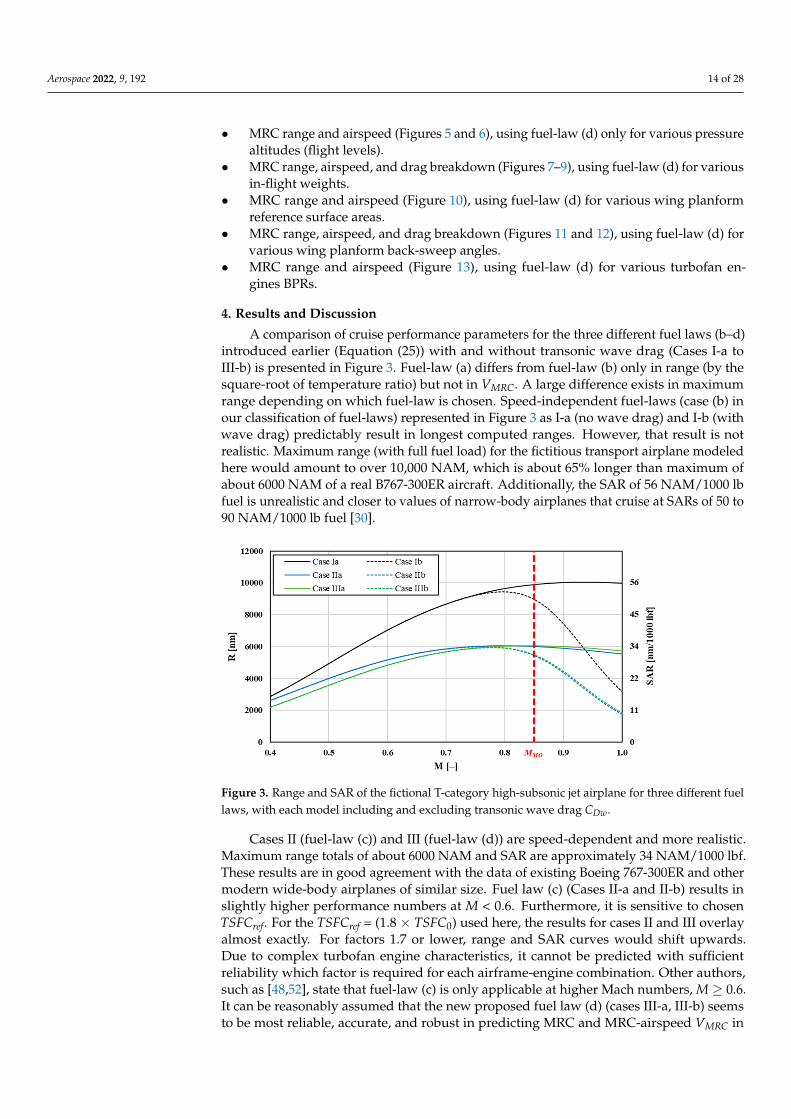
A comparison of cruise performance parameters for the three different fuel laws (b–d)introduced earlier (Equation (25)) with and without transonic wave drag (Cases I-a toIII-b) is presented in Figure 3. Fuel-law (a) differs from fuel-law (b) only in range (by thesquare-root of temperature ratio) but not in VMRC. A large difference exists in maximumrange depending on which fuel-law is chosen. Speed-independent fuel-laws (case (b) inour classification of fuel-laws) represented in Figure 3 as I-a (no wave drag) and I-b (withwave drag) predictably result in longest computed ranges. However, that result is notrealistic. Maximum range (with full fuel load) for the fictitious transport airplane modeledhere would amount to over 10,000 NAM, which is about 65% longer than maximum ofabout 6000 NAM of a real B767-300ER aircraft. Additionally, the SAR of 56 NAM/1000 lbfuel is unrealistic and closer to values of narrow-body airplanes that cruise at SARs of 50 to90 NAM/1000 lb fuel [30].


about 6000 NAM of a real B767-300ER aircraft. Additionally, the SAR of 56 NAM/1,000 lb fuel is unrealistic and closer to values of narrow-body airplanes that cruise at SARs of 50 to 90 NAM/1,000 lb fuel [30].

Figure 3. Range and SAR of the fictional T-category high-subsonic jet airplane for three different fuel laws, with each model including and excluding transonic wave drag CDw.

Cases II (fuel-law (c)) and III (fuel-law (d)) are speed-dependent and more realistic. Maximum range totals of about 6000 NAM and SAR are approximately 34 NAM/1,000 lbf. These results are in good agreement with the data of existing Boeing 767-300ER and other modern wide-body airplanes of similar size. Fuel law (c) (Cases II-a and II-b) results in slightly higher performance numbers at M < 0.6. Furthermore, it is sensitive to chosen TSFCref. For the TSFCref = (1.8 × TSFC0) used here, the results for cases II and III overlay almost exactly. For factors 1.7 or lower, range and SAR curves would shift upwards. Due to complex turbofan engine characteristics, it cannot be predicted with sufficient reliabil-ity which factor is required for each airframe-engine combination. Other authors, such as [48,52], state that fuel-law (c) is only applicable at higher Mach numbers, M ≥ 0.6. It can be reasonably assumed that the new proposed fuel law (d) (cases III-a, III-b) seems to be most reliable, accurate, and robust in predicting MRC and MRC-airspeed VMRC in the en-tire flight envelope. Subsequent investigations into the influence of dynamic input param-eters will therefore be mostly conducted using this new proposed fuel-law.

One can observe from Figure 3 an expected decrease in the maximum range in all cases when transonic wave drag model is included. Results start to diverge upon reaching MCR, which in these cases is around 0.75. One can also observe relatively flat maximums, meaning that small speed variations around MRC do not affect still-air range much. Range change for speed-independent fuel law (b) is quite severe but still overpredicts range in comparison with the speed-dependent fuel laws. This is not surprising as the maximum for case I-a is located deep in the transonic speed range close to M = 1. Once wave-drag is accounted for, maximum range for cases II and III occurs at lower airspeeds of approxi-mately M ≈ 0.8. It must be stated that the transonic wave-drag model becomes increasingly inaccurate as the freestream flight Mach number increases and especially as the upper boundary of transonic regime (M = 1.2) is approached. In the upper transonic region, shocks become stronger. However, we are only interested in the wave-drag at the lower end of the transonic region. Additionally, for all three cases, VMRC decreases when the wave-drag is included. The difference is largest for fuel law “b” (−15%) and least for “c” (−4.2%) as it exhibits the earliest maximum in the range. For the fuel-law “d”, wave drag penalty on VMRC is negative 7.2%. The exact data for fuel law comparison for the fictitious T-category airplane are summarized in Table 4 and Figure 4. Apparently, transonic wave drag has more effect on the VMRC/MMRC than on cruise range (MRC) itself. For all cases,

Figure 3. Range and SAR of the fictional T-category high-subsonic jet airplane for three different fuellaws, with each model including and excluding transonic wave drag CDw.

Cases II (fuel-law (c)) and III (fuel-law (d)) are speed-dependent and more realistic.Maximum range totals of about 6000 NAM and SAR are approximately 34 NAM/1000 lbf.These results are in good agreement with the data of existing Boeing 767-300ER and othermodern wide-body airplanes of similar size. Fuel law (c) (Cases II-a and II-b) results inslightly higher performance numbers at M < 0.6. Furthermore, it is sensitive to chosenTSFCref. For the TSFCref = (1.8 × TSFC0) used here, the results for cases II and III overlayalmost exactly. For factors 1.7 or lower, range and SAR curves would shift upwards.Due to complex turbofan engine characteristics, it cannot be predicted with sufficientreliability which factor is required for each airframe-engine combination. Other authors,such as [48,52], state that fuel-law (c) is only applicable at higher Mach numbers, M ≥ 0.6.It can be reasonably assumed that the new proposed fuel law (d) (cases III-a, III-b) seemsto be most reliable, accurate, and robust in predicting MRC and MRC-airspeed VMRC in

Aerospace 2022, 9, 192 15 of 28

the entire flight envelope. Subsequent investigations into the influence of dynamic inputparameters will therefore be mostly conducted using this new proposed fuel-law.

One can observe from Figure 3 an expected decrease in the maximum range in allcases when transonic wave drag model is included. Results start to diverge upon reachingMCR, which in these cases is around 0.75. One can also observe relatively flat maximums,meaning that small speed variations around MRC do not affect still-air range much. Rangechange for speed-independent fuel law (b) is quite severe but still overpredicts range incomparison with the speed-dependent fuel laws. This is not surprising as the maximumfor case I-a is located deep in the transonic speed range close to M = 1. Once wave-drag is accounted for, maximum range for cases II and III occurs at lower airspeeds ofapproximately M ≈ 0.8. It must be stated that the transonic wave-drag model becomesincreasingly inaccurate as the freestream flight Mach number increases and especially asthe upper boundary of transonic regime (M = 1.2) is approached. In the upper transonicregion, shocks become stronger. However, we are only interested in the wave-drag atthe lower end of the transonic region. Additionally, for all three cases, VMRC decreaseswhen the wave-drag is included. The difference is largest for fuel law “b” (−15%) andleast for “c” (−4.2%) as it exhibits the earliest maximum in the range. For the fuel-law“d”, wave drag penalty on VMRC is negative 7.2%. The exact data for fuel law comparisonfor the fictitious T-category airplane are summarized in Table 4 and Figure 4. Apparently,transonic wave drag has more effect on the VMRC/MMRC than on cruise range (MRC) itself.For all cases, MRC is obtained at airspeeds closer to drag-divergence Mach number thanminimum-drag airspeed (VMD/MMD). Maximum cruise range MMRC at high altitudes isusually 10–32% greater than MMD and located in transonic range. As fuel law (d) was nowidentified to deliver most robust results, subsequent analysis here will only consider thatfuel law. Analytical and polynomial MRC airspeeds and ranges for fuel-laws (a), (b), and(c) are summarized in Appendix A.


MRC is obtained at airspeeds closer to drag-divergence Mach number than minimum-drag airspeed (VMD/MMD). Maximum cruise range MMRC at high altitudes is usually 10–32% greater than MMD and located in transonic range. As fuel law (d) was now identified to deliver most robust results, subsequent analysis here will only consider that fuel law. An-alytical and polynomial MRC airspeeds and ranges for fuel-laws (a), (b), and (c) are sum-marized in Appendix A.

Table 4. Fuel law-dependence of MRC and MRC Mach number (MMRC) for both cases, with and without transonic wave-drag model.

MRC (Case I)

MRC (Case II)

MRC (Case III)

MMRC (Case I)

MMRC

(Case II) MMRC

(Case III) Without

wave drag 10,036 nm 6055 nm 6049 nm 0.935 0.797 0.838

With wave drag

9440 nm (−5.9%)

6005 nm (−0.8%)

5931 nm (−1.9%)

0.797 (−14.8%)

0.763 (−4.2%)

0.778 (−7.2%)

Figure 4. MRC and MRC airspeed for three fuel-laws tested—(b), (c), and (d)—for both cases, with and without transonic wave-drag model.

The numerical computations were performed for flight-level (FL) increments of 5000 ft (1500 m) starting at 5000 ft. Results reveal a tendency towards higher achievable range at greater altitudes and at increased airspeeds (>+40%). Wave drag must be taken into account only at typical cruise levels because, for the fictional T-category airplane modeled here, MMRC < MCR until up to about 28,000 ft. For flight levels where wave drag is present, it comes as no surprise that both range and MRC airspeed are located below the results when transonic wave drag is neglected. SAR changes from 22.5 NAM/1000 lb at 5000 ft to almost 33 NAM/1000 lb at FL330.

Figure 5 illustrates the behavior in the familiar two-dimensional layout, while Figure 6 resorts to a three-dimensional plot. Here, one can rapidly identify that maximum range occurs at the highest flight altitudes and at Mach numbers around 0.8. No confidence ex-ists for the results exceeding flight Mach numbers of about 0.94 for the present model.

Figure 4. MRC and MRC airspeed for three fuel-laws tested—(b), (c), and (d)—for both cases, withand without transonic wave-drag model.

Table 4. Fuel law-dependence of MRC and MRC Mach number (MMRC) for both cases, with andwithout transonic wave-drag model.

MRC(Case I)

MRC(Case II)

MRC(Case III)

MMRC(Case I)

MMRC(Case II)

MMRC(Case III)

Withoutwave drag 10,036 nm 6055 nm 6049 nm 0.935 0.797 0.838

With wavedrag

9440 nm 6005 nm 5931 nm 0.797 0.763 0.778(−5.9%) (−0.8%) (−1.9%) (−14.8%) (−4.2%) (−7.2%)

Aerospace 2022, 9, 192 16 of 28

The numerical computations were performed for flight-level (FL) increments of 5000 ft(1500 m) starting at 5000 ft. Results reveal a tendency towards higher achievable rangeat greater altitudes and at increased airspeeds (>+40%). Wave drag must be taken intoaccount only at typical cruise levels because, for the fictional T-category airplane modeledhere, MMRC < MCR until up to about 28,000 ft. For flight levels where wave drag is present,it comes as no surprise that both range and MRC airspeed are located below the resultswhen transonic wave drag is neglected. SAR changes from 22.5 NAM/1000 lb at 5000 ft toalmost 33 NAM/1000 lb at FL330.

Figure 5 illustrates the behavior in the familiar two-dimensional layout, while Figure 6resorts to a three-dimensional plot. Here, one can rapidly identify that maximum rangeoccurs at the highest flight altitudes and at Mach numbers around 0.8. No confidence existsfor the results exceeding flight Mach numbers of about 0.94 for the present model.


Figure 5. MMRC and range for different FLs for both models, with/without wave drag.

Figure 6. 3D plot visualizing the influence of altitude and Mach on range with transonic wave drag model.

Further investigations were conducted for clean cruise configurations at FL330 and variable in-flight weight. Reducing in-flight weight while keeping fuel capacity constant naturally leads to increased range due to reduced vortex drag. B767-300ER with a take-off and fuel weight of about 410,000 lb and 160,000 lb, respectively, has a usable fuel fraction of 39%. This is in the range of modern transport commercial jets, which have a fuel-weight ratio of less than half their maximum structural take-off weights (about 26% for medium-haul and 45% for long-haul planes). Maximum range decreases with increased in-flight weight, and MMRC is evaluated for both drag models, including and excluding wave drag, as shown in Figure 7. The relationship between the 1-g flight CL and Mach at given weight and altitude (pressure ratio) is:




Figure 6. 3D plot visualizing the influence of altitude and Mach on range with transonic wave drag model.

Further investigations were conducted for clean cruise configurations at FL330 and variable in-flight weight. Reducing in-flight weight while keeping fuel capacity constant naturally leads to increased range due to reduced vortex drag. B767-300ER with a take-off and fuel weight of about 410,000 lb and 160,000 lb, respectively, has a usable fuel fraction of 39%. This is in the range of modern transport commercial jets, which have a fuel-weight ratio of less than half their maximum structural take-off weights (about 26% for medium-haul and 45% for long-haul planes). Maximum range decreases with increased in-flight weight, and MMRC is evaluated for both drag models, including and excluding wave drag, as shown in Figure 7. The relationship between the 1-g flight CL and Mach at given weight and altitude (pressure ratio) is:

Figure 6. 3D plot visualizing the influence of altitude and Mach on range with transonic wavedrag model.

Aerospace 2022, 9, 192 17 of 28

Further investigations were conducted for clean cruise configurations at FL330 andvariable in-flight weight. Reducing in-flight weight while keeping fuel capacity constantnaturally leads to increased range due to reduced vortex drag. B767-300ER with a take-offand fuel weight of about 410,000 lb and 160,000 lb, respectively, has a usable fuel fraction of39%. This is in the range of modern transport commercial jets, which have a fuel-weightratio of less than half their maximum structural take-off weights (about 26% for medium-haul and 45% for long-haul planes). Maximum range decreases with increased in-flightweight, and MMRC is evaluated for both drag models, including and excluding wave drag,as shown in Figure 7. The relationship between the 1-g flight CL and Mach at given weightand altitude (pressure ratio) is:

M2CL ∝Wδ

(32)


2LWM Cδ

∝ (32)

Figure 7. MMRC and range for variable in-flight weight for both drag models, with and without tran-sonic wave drag.

In-depth analysis would show that the maximum still-air range will be obtained by maintaining the product M2 × CL constant, which, for decreasing in-flight weight (due to fuel consumption), will require an airplane to climb continuously at low climb rates (15–25 feet/minute). Since ATC separation traffic restrictions do not allow continuous-climb flight (except for famed Concorde’s continuous-climb at supersonic speeds), the next best thing is step-climb, which is an accepted operational practice made more feasible by in-troduction of RVSM [30]. 3D plot illustrating dependance of range on flight Mach number and in-flight weight is presented in Figure 8. When transonic shock systems are present, VMRC rises to certain point. After passing “critical weight” condition, best cruise airspeed stays almost constant and decreases only slightly with increased weight. The reason for is the increasing transonic wave-drag coefficient with increasing Mach number. In cases where transonic wave drag was neglected, VMRC increases almost linearly while range de-creases. Graphical representation of drag counts as a function of weight is shown with a bar-graph in Figure 9. Even at highest weights, transonic wave drag is a very small pro-portion of the total drag (less than 5%).

Figure 7. MMRC and range for variable in-flight weight for both drag models, with and withouttransonic wave drag.

In-depth analysis would show that the maximum still-air range will be obtained bymaintaining the product M2 × CL constant, which, for decreasing in-flight weight (dueto fuel consumption), will require an airplane to climb continuously at low climb rates(15–25 feet/minute). Since ATC separation traffic restrictions do not allow continuous-climb flight (except for famed Concorde’s continuous-climb at supersonic speeds), thenext best thing is step-climb, which is an accepted operational practice made more feasibleby introduction of RVSM [30]. 3D plot illustrating dependance of range on flight Machnumber and in-flight weight is presented in Figure 8. When transonic shock systems arepresent, VMRC rises to certain point. After passing “critical weight” condition, best cruiseairspeed stays almost constant and decreases only slightly with increased weight. Thereason for is the increasing transonic wave-drag coefficient with increasing Mach number.In cases where transonic wave drag was neglected, VMRC increases almost linearly whilerange decreases. Graphical representation of drag counts as a function of weight is shownwith a bar-graph in Figure 9. Even at highest weights, transonic wave drag is a very smallproportion of the total drag (less than 5%).

Aerospace 2022, 9, 192 18 of 28


Figure 8. 3D plot visualizing influence of in-flight weight and Mach number on the range, including transonic wave drag.

Figure 9. Drag breakdown for a simulated fictitious T-category aircraft, depending on in-flight cruise weight.

An overview of percentage variations of maximum range and corresponding best cruise airspeed is summarized in Table 5. It can be concluded that lift-dependent wave drag component has significant impact on cruise performance for heavy aircraft.

Table 5. Weight-dependence of maximum range and maximum-range airspeed, for both cases, with and without wave drag (including/excluding wave drag).

W [1000 lb] 300 340 380 420 460 500 Mach (M)

No wave drag 0.731 0.776 0.818 0.857 0.895 0.931

Mach (M) With wave drag

0.731 −0.0%

0.766 −1.3%

0.776 −5.1%

0.778 −9.2%

0.777 −13.2%

0.774 −16.9%

Figure 8. 3D plot visualizing influence of in-flight weight and Mach number on the range, includingtransonic wave drag.


Figure 8. 3D plot visualizing influence of in-flight weight and Mach number on the range, including transonic wave drag.

Figure 9. Drag breakdown for a simulated fictitious T-category aircraft, depending on in-flight cruise weight.

An overview of percentage variations of maximum range and corresponding best cruise airspeed is summarized in Table 5. It can be concluded that lift-dependent wave drag component has significant impact on cruise performance for heavy aircraft.

Table 5. Weight-dependence of maximum range and maximum-range airspeed, for both cases, with and without wave drag (including/excluding wave drag).

W [1000 lb] 300 340 380 420 460 500 Mach (M)

No wave drag 0.731 0.776 0.818 0.857 0.895 0.931

Mach (M) With wave drag

0.731 −0.0%

0.766 −1.3%

0.776 −5.1%

0.778 −9.2%

0.777 −13.2%

0.774 −16.9%

Figure 9. Drag breakdown for a simulated fictitious T-category aircraft, depending on in-flightcruise weight.

An overview of percentage variations of maximum range and corresponding bestcruise airspeed is summarized in Table 5. It can be concluded that lift-dependent wavedrag component has significant impact on cruise performance for heavy aircraft.

Aerospace 2022, 9, 192 19 of 28

Table 5. Weight-dependence of maximum range and maximum-range airspeed, for both cases, withand without wave drag (including/excluding wave drag).

W [1000 lb] 300 340 380 420 460 500

Mach (M)No wave drag 0.731 0.776 0.818 0.857 0.895 0.931

Mach (M) 0.731 0.766 0.776 0.778 0.777 0.774With wave drag −0.0% −1.3% −5.1% −9.2% −13.2% −16.9%

Range (R)No wave drag 8080 nm 7088 nm 6352 nm 5778 nm 5316 nm 4934 nm

Range (R) 8080 nm 7081 nm 6285 nm 5597 nm 4982 nm 4426 nmNo wave drag −0.0% −0.1% −1.0% −3.1% −6.3% −10.3%

Discussion of third input parameter wing reference surface area shows that increasingsurface area results in progressively lower maximum range as well as lower airplane’s bestcruise speed for both models including and excluding wave drag. Larger wing surfaceareas effectively reduce lift coefficient CL and cause later drag rise (higher MDD). On theother hand, larger wing wetted area creates more parasitic drag so that most economiccruise airspeed essentially moves to lower speeds. Interestingly, wave drag only comesinto account for smaller wing areas because for larger lifting surfaces VMRC is shifted intosubcritical subsonic region (M < MCR). Consequently, no wave drag can form, and thecurves for both models are identical as plotted in Figure 10.


Range (R) No wave drag 8080 nm 7088 nm 6352 nm 5778 nm 5316 nm 4934 nm

Range (R) No wave drag

8080 nm −0.0%

7081 nm −0.1%

6285 nm −1.0%

5597 nm −3.1%

4982 nm −6.3%

4426 nm −10.3%

Discussion of third input parameter wing reference surface area shows that increas-ing surface area results in progressively lower maximum range as well as lower airplane’s best cruise speed for both models including and excluding wave drag. Larger wing sur-face areas effectively reduce lift coefficient CL and cause later drag rise (higher MDD). On the other hand, larger wing wetted area creates more parasitic drag so that most economic cruise airspeed essentially moves to lower speeds. Interestingly, wave drag only comes into account for smaller wing areas because for larger lifting surfaces VMRC is shifted into subcritical subsonic region (M < MCR). Consequently, no wave drag can form, and the curves for both models are identical as plotted in Figure 10.

Figure 10. MMRC and range over wing surface area for both models, including and excluding CDw.

If transonic-flow normal shocks are ignored, the sweep-angle Λ parameter does not change the total drag significantly. Range and maximum cruise range airspeed remain constant in that case, as shown in Figure 11. With wave drag included, increasing leading-edge sweep delays critical flow conditions on the wing’s upper surface to higher Mach numbers as the LE perpendicular velocity component diminishes. A good example is Con-corde, which, although flying supersonically, had subsonic double-ogee wing planform. Thereby, CDw decreases and efficient flight at higher forward speeds is enabled. Accord-ingly, both VMRC and range also increase steadily with Λ (MDD increases with increasing sweep angle according to modified Korn equation). Wave drag decreases with increased sweep, a relation that is noticeable also with the drag proportions in Figure 12 and range and MMRC data presented in Table 6.

Figure 10. MMRC and range over wing surface area for both models, including and excluding CDw.

If transonic-flow normal shocks are ignored, the sweep-angle Λ parameter does notchange the total drag significantly. Range and maximum cruise range airspeed remainconstant in that case, as shown in Figure 11. With wave drag included, increasing leading-edge sweep delays critical flow conditions on the wing’s upper surface to higher Machnumbers as the LE perpendicular velocity component diminishes. A good example isConcorde, which, although flying supersonically, had subsonic double-ogee wing planform.Thereby, CDw decreases and efficient flight at higher forward speeds is enabled. Accordingly,both VMRC and range also increase steadily with Λ (MDD increases with increasing sweepangle according to modified Korn equation). Wave drag decreases with increased sweep, arelation that is noticeable also with the drag proportions in Figure 12 and range and MMRCdata presented in Table 6.

Aerospace 2022, 9, 192 20 of 28


Figure 11. MMRC and range for variable sweep angle Λ for both models, with and without CDw.

Figure 12. Drag breakdown of a fictitious T-category airplane as a function of sweep angle Λ.

Table 6. Maximum range and best cruise airspeed for both models, with and without wave drag.

Λ [degree] 10° 15° 20° 25° 30° 35° 40° M [-]

No CDw 0.838

M [-] With CDw

0.707 −15.6%

0.715 −14.7%

0.725 −13.4%

0.740 −11.7%

0.757 −9.6%

0.778 −7.2%

0.800 −4.5%

R [NAM] No CDw

6049 nm (11,200 km)

R [NAM] With CDw

5554 −8.2%

5608 −7.3%

5679 −6.1%

5762 −4.7%

5849 −3.3%

5931 −1.9%

5995 −0.9%






Λ [degree] 10° 15° 20° 25° 30° 35° 40° M [-]

No CDw 0.838

M [-] With CDw

0.707 −15.6%

0.715 −14.7%

0.725 −13.4%

0.740 −11.7%

0.757 −9.6%

0.778 −7.2%

0.800 −4.5%

R [NAM] No CDw

6049 nm (11,200 km)

R [NAM] With CDw

5554 −8.2%

5608 −7.3%

5679 −6.1%

5762 −4.7%

5849 −3.3%

5931 −1.9%

5995 −0.9%



Λ [degree] 10 15 20 25 30 35 40

M [-]No CDw

0.838

M [-] 0.707 0.715 0.725 0.740 0.757 0.778 0.800With CDw −15.6% −14.7% −13.4% −11.7% −9.6% −7.2% −4.5%

R [NAM]No CDw

6049 nm (11,200 km)

R [NAM] 5554 5608 5679 5762 5849 5931 5995With CDw −8.2% −7.3% −6.1% −4.7% −3.3% −1.9% −0.9%

Aerospace 2022, 9, 192 21 of 28

The last input parameter evaluated here is BPR of turbofan engines. Aircrafts equippedwith powerplants with higher BPR tend to achieve greater range due to lower TSFC.However, the airspeed VMRC at which optimum range is reached stays almost constant forHBPR (High BPR) and UHBPR (Ultra-High BPR) engines. At high Mach numbers between0.8 and 0.9, UHBPR turbofans show a larger thrust decrease due to ram effect than HBPRengines. Cruise altitudes such as FL330 result in only a minor difference in thrust availablefor both turbofan types, and consequently both VMRC are nearly identical. If one considersother engines than the P&Ws PW4056 modeled here with Equation (24), a greater BPRwould accentuate the trend towards better range performance. The higher the BPR, thehigher maximum range at still almost constant MMRC, as shown in Figure 13.


The last input parameter evaluated here is BPR of turbofan engines. Aircrafts equipped with powerplants with higher BPR tend to achieve greater range due to lower TSFC. However, the airspeed VMRC at which optimum range is reached stays almost con-stant for HBPR (High BPR) and UHBPR (Ultra-High BPR) engines. At high Mach numbers between 0.8 and 0.9, UHBPR turbofans show a larger thrust decrease due to ram effect than HBPR engines. Cruise altitudes such as FL330 result in only a minor difference in thrust available for both turbofan types, and consequently both VMRC are nearly identical. If one considers other engines than the P&Ws PW4056 modeled here with Equation (24), a greater BPR would accentuate the trend towards better range performance. The higher the BPR, the higher maximum range at still almost constant MMRC, as shown in Figure 13.

Figure 13. Range and SAR of the fictitious T-category airplane as a function of BPR and Mach num-ber for both models, including and excluding wave drag.

All previous computations and optimizations were made for the AEO (All Engines Operating) cruise scenarios. OEI (One Engine Inoperative) conditions were treated for all input parameters, but it was found that they do not require separate presentation as the maximum level airspeeds when OEI are significantly lower than for the AEO cases. Sud-den engine failure in flight is not a particularly serious problem as the aircraft will con-tinue to fly; however, a drift-down must be initiated toward OEI-service ceiling (typically 22,000–25,000 ft) where flight at constant airspeed can be maintained with remaining op-erating engine(s). OEI maximum range cruise airspeed will no longer be in transonic re-gion and hence no wave drag is present. Additionally, flight may proceed to unscheduled nearest acceptable airport. For more details on optimal subsonic airspeeds and range dur-ing OEI conditions, one can resort to [31].

Looking at the fictional aircraft modeled here with MTOW of 400,000 lb, sweep of 35°, wing area of 3100 ft2 and in cruise at FL330, wave drag accounts for only 1% of the total drag when flying at MRC Mach number of about 0.78. Drag breakdowns are also shown in Figures 9 and 12. However, many references estimate the transonic wave drag component for transport airplanes flown at cruise M below MDD at about 5% of the total drag [53,54]. This discrepancy cannot be ascribed to deficiencies of the mathematical model but finds its origin primarily in two contributing factors. Firstly, the sweep angle of 35° used here is rather high. Real B767-300ER, A350, and similar T-category airplanes feature leading edges with angles of 31.5 to 32°. Secondly, long-range jetliners will nor-mally cruise at speeds faster than MMRC. The cost index (CI) is practically never zero in

Figure 13. Range and SAR of the fictitious T-category airplane as a function of BPR and Mach numberfor both models, including and excluding wave drag.

All previous computations and optimizations were made for the AEO (All EnginesOperating) cruise scenarios. OEI (One Engine Inoperative) conditions were treated forall input parameters, but it was found that they do not require separate presentation asthe maximum level airspeeds when OEI are significantly lower than for the AEO cases.Sudden engine failure in flight is not a particularly serious problem as the aircraft willcontinue to fly; however, a drift-down must be initiated toward OEI-service ceiling (typi-cally 22,000–25,000 ft) where flight at constant airspeed can be maintained with remainingoperating engine(s). OEI maximum range cruise airspeed will no longer be in transonicregion and hence no wave drag is present. Additionally, flight may proceed to unschedulednearest acceptable airport. For more details on optimal subsonic airspeeds and rangeduring OEI conditions, one can resort to [31].

Looking at the fictional aircraft modeled here with MTOW of 400,000 lb, sweep of35, wing area of 3100 ft2 and in cruise at FL330, wave drag accounts for only 1% of thetotal drag when flying at MRC Mach number of about 0.78. Drag breakdowns are alsoshown in Figures 9 and 12. However, many references estimate the transonic wave dragcomponent for transport airplanes flown at cruise M below MDD at about 5% of the totaldrag [53,54]. This discrepancy cannot be ascribed to deficiencies of the mathematical modelbut finds its origin primarily in two contributing factors. Firstly, the sweep angle of 35

used here is rather high. Real B767-300ER, A350, and similar T-category airplanes featureleading edges with angles of 31.5 to 32. Secondly, long-range jetliners will normally cruiseat speeds faster than MMRC. The cost index (CI) is practically never zero in flight operations,and time-cost (crew time, etc.) plays an important role in finding best-economy airspeed.Flying with effective headwinds will require faster forward airspeeds to maximize range

Aerospace 2022, 9, 192 22 of 28

over ground or SGR [30]. While MMRC does not account for wind, economy-Mach (MECON)does. Modern T-category jets are sometimes flown at the long-range-cruise airspeed (MLRC)industry standard, which is based on the 99% MRC, which corresponds to somewhat higherLRC airspeeds (MLRC is typically MMRC + 0.02). For our fictious airplane model, MMRCis 0.78 so that MLRC could be about 0.80 (which also happens to be design cruise Machof B767-300). Wave drag and the total CD for new sweep and forward airspeed wouldamount to 0.00148 and 0.03395, respectively. Wave drag proportion of the total drag isnow 4.4% and close to the usual cited figures of 5% for high-subsonic wide-body airplanes,again validating the accuracy of the approach in this study. Using Flight ManagementSystems (FMS), the operational airspeeds are economy Mach numbers, which minimizestotal operating cost (fuel-cost and time-dependent cost). For more details on cruise speeds,ranges, and economy, see [30].

Maximum operating limit airspeeds in flight operations VMO/MMO are based on flighttesting and are established in relationship to design diving airspeed VD/MD, maximumflight demonstrated diving airspeed VDF/MDF, and the maximum airspeed for stabilitycharacteristics VFC/MFC. Some of the corresponding regulations in US are Title 14 ofCFR 25.253 (high-speed characteristics), CFR 25.335 (design airspeeds), and CFR 25.1505(maximum operating limit airspeed). Maximum operating limit airspeed is limited by max-q (at lower altitudes) and generally by aircraft static and dynamic stability, control, handlingqualities, upset recovery, structural integrity, flutter, vibrations, loads, and other limitations.More on this subject and airworthiness requirements of FAR and CS 25 airplanes can befound in [55–57]. Range is computed and summarized in Table 7 for various aerodynamic,performance, control, and operationally limiting airspeeds for an airplane similar to B767-300 (check Tables 1–3). Approximate operational cost index (CI) for a typical range 0–200(in older FMSs) was given as a reference. In these conditions, critical Mach number is about0.75 with the wave drag being zero. Still-air range at MCR is lower than at MMRC. Values ofwave drag proportion, airspeeds, and ranges agree well with the certified and flight-testedvalues for T-category airplanes of similar designs, demonstrating that modeling used hereis reasonably accurate.

Table 7. Flight Mach, maximum still-air range, and wave-drag percentage of the total drag for variousflight conditions at constant in-flight weight of 350,000 lb flying at 35,000 ft ISA.

M > MCRMMRC MLRC MECON MDD MMOCI = 0 CI ≈ 30–40 CI ≈ 80 CI ≈ 140 CI ≈ 200

FlightMach [-] 0.77 0.78 0.80 0.82 0.84 0.85

Air-Range[NAM]

7006 nm 7010 6950 6857 6655 6488−0.06% −0.14% −1.0% −2.18% −5.06% −7.47%

Wave Drag[%] 0.41% 0.71 1.88 3.37 6.15 8.38

It must be underscored again that transonic wave-drag represents complicated flowphenomenon that cannot be fully described by a relatively simple semi-empirical algebraicmodel in the supercritical flight regime as used here. For Mach numbers between MCRand MMO as investigated in this study, the proposed semi-empirical wave-drag, fuel-law,and turbofan models are still reasonably satisfactory and could be used to develop basicmethodology for design optimization in early aircraft development phases. During suchinitial phase, other performance airspeeds under control of wave-drag can be estimatedwith the present model, such as the maximum level-flight propulsion-limited airspeed.Computations of propulsion-limited maximum level flight airspeeds may be presented ina separate publication. It is also emphasized that this is perhaps one of several possiblemethodologies of estimating cruise parameters of modern transonic airplanes. The resultsobtained here show reasonable agreement with demonstrated flight data. Further improve-

Aerospace 2022, 9, 192 23 of 28

ments in models are possible and are envisioned. Present algebraic models could be, intheory, extended to account for supersonic flight of various aerospace designs. One of thebiggest difficulties in presented method is in choosing a wing-technology factor for a givendesign as no rational analysis for that currently exists.

5. Conclusions

Transonic wave-drag computations using modern RANS/LES/DNS codes is time,cost, and resource consuming. Thus, in this article a semi-empirical wave-drag model forsupercritical flow was developed and subsequently added to the standard compressiblesubcritical parabolic drag polar in the linear lift region. The wave drag model developed isincreasingly inaccurate for Mach numbers approaching one and should be fully discardedfor Mach numbers on supersonic side of the transonic regime. Luckily, only the subsonicside of the transonic supercritical flow around the drag-divergence Mach number wasneeded. The criterion of maximizing the specific air range (SAR) was developed. Optimalitycriterion delivers polynomials, whose analytical and numerical solutions agree well with theknown cruise range and airspeed results of modern commercial T-category jets. New semi-empirical turbofan model and fuel-laws were implemented, giving rise to polynomials of12th and higher orders. A numerical Newton–Raphson nonlinear equation solver code wasdeveloped and used for all computations. The NR algorithm searched only for positive realroots of polynomials representing the sought-after optimum airspeeds. The NR method andcode were extensively tested against known analytical cruise range solutions to guaranteeaccuracy and convergence. Cruise range is calculated by analytical or numerical integrationof Breguet range equation while utilizing several fuel-flow laws for comparison. It wasfound that transonic shock systems have a noticeable influence on cruise range parameters.The dependence of performance airspeeds on several design features was explored for aspecific airframe-powerplant vehicle and various atmospheric cruise conditions.

The numerical method used can be applied to all other drag polynomials, includingeventual non-integer exponents. If available, wind tunnel-, flight-test-, or CFD-obtainedtransonic drag polars can be incorporated into methodology developed. The model usedhere allows turbofan characteristics in any suitable polynomial form. It can be utilized toidentify the most beneficial input parameter values and combinations for the cruise flightphase, especially regarding geometric airframe data. The algorithm represents a powerfultool to estimate important performance airspeeds in transonic flights on the subsonicside. Its intended application is utilization in the conceptual development stages of thedesign optimization of high-subsonic jet airplanes. The results may also assist in improvingoperational techniques and best piloting practices in modern air transportation. Furtherimprovements of this integral algebraic model are certainly possible and are planned.

Author Contributions: Conceptualization, N.E.D.; Data curation, J.W.; Formal analysis, N.E.D.;Investigation, J.W.; Methodology, J.W. and N.E.D.; Software, J.W.; Supervision, N.E.D.; Writing—original draft, N.E.D.; Writing—review & editing, J.W. All authors have read and agreed to thepublished version of the manuscript.

Funding: No external funding was involved in this study.

Institutional Review Board Statement: Not applicable.

Informed Consent Statement: Not applicable.

Data Availability Statement: Not applicable.

Conflicts of Interest: The authors declare no conflict of interest.

Aerospace 2022, 9, 192 24 of 28

Glossary

Symbolsa Speed of Sound [m/s]c Chord (airfoil) [m]CD Coefficient of drag [-]Ci Coefficient of induced drag [-]CL Coefficient of lift [-]Cp Coefficient of pressure [-]Cp Coefficient of parasitic drag [-]Cw Coefficient of wave drag [-]D Drag force [N]f Coefficient in modified Lock’s equation [-]h Enthalpy (specific) [kJ/kg]K Coefficient of drag not-due-to-lift [-]L Lift force [N]m Exponent in modified Lock’s equation [-]M Mach number [-]n Load factor [-]n Exponent (fuel law) [-]p Pressure [Pa]Re Reynolds number [-]s Entropy (specific) [kJ/kg K]t Time [s]t Thickness (airfoil) [m]T Temperature (absolute) [K]T Thrust force [N]v Airspeed (true) [m/s]W Weight [N]z Coefficient in modified Lock’s equation [-]Notea, b, c, d, e Dummy coefficients (Equation (17))A, B, C, D, E, F, G, H, I, J, K, M, N Dummy coefficients (Equation (19))Greekα Angle of attack [radian or degree]β Compressibility correction factor [-]β Sideslip angle [radian or degree]φ Potential function (velocity)Φ Potential function (velocity)γ Coefficient of isentropic expansion [-]κA Wing technology factor in Korn’s equation [-]κ Wing slope factor in Korn’s equation [-]ρ Density (air) [kg/m3]Λ Sweep angle (wing) [radian or angular degree]θ Relative temperature (air) [-]σ Relative density (air) [-]ς Vorticity [rad/s]SubscriptsCR CriticalDD Drag divergenceDW Wave drag (transonic)LE Leading edgeref ReferenceSL Sea Leveltot Total

Aerospace 2022, 9, 192 25 of 28

AbbreviationsAEO All Engines OperatingAOA Angle-of-AttackATC Air Traffic ControlBL Boundary LayerBPR Bypass Ratio (turbofan engines)CFD Computational Fluid DynamicsCFR Code of Federal Regulation (FAA, Title 14 CFR)CI Cost IndexCS Certification Specifications (EASA)DES Detached Eddy SimulationDNS Direct Navier–Stokes simulationsEASA European Union Aviation Safety AgencyECON Economy cruise based on CIFAA Federal Aviation Administration (US Department of Transportation agency)FAR Federal Aviation Regulations (Tile 14 CFR, FAA)FL Flight Level (pressure altitude in hundreds of feet or meter)FMS Flight Management SystemHBPR High Bypass Ratio (turbofan engines)ICAO International Civil Aviation OrganizationISA International Standard AtmosphereLEO Low Earth OrbitLES Large-Eddy SimulationLRC Long Range CruiseMCT Maximum Continuous ThrustMO Maximum Operating (subscript)MRC Maximum Range CruiseNAM Nautical Air Miles (still-air nautical miles)NR Newton–Raphson nonlinear equations solverNS Navier–StokesOEI One Engine InoperativePDE Partial Differential EquationsRANS Reynolds-averaged Navier–Stokes equationsRBCC Rocket-Based Combined CycleRF Range FactorRVSM Reduced Vertical Separation Minimum (ICAO)SAR Specific Air Range (still-air)SGR Specific Ground Range (accounting for wind)S&L Straight and Level (cruise) flightSSTO Single-Stage to OrbitSWBLI Shock-Wave Boundary-Layer InteractionsTOGA Takeoff/Go-Around ThrustTSFC Thrust Specific Fuel ConsumptionUHBPR Ultra-High Bypass Ratio (turbofan engines)URANS Unsteady Reynolds-averaged Navier–Stokes

Appendix A. Other Fuel Laws

In the main text, all MRC range and airspeed computations and parameter variationsutilized fuel-law (d). Analytic expressions for MMRC using fuel-laws (a), (b), and (c) arepresented here. Some analytical expressions for MRC cruise parameters exist in case wave-drag is neglected and for simple fuel-laws. General differential equation for the optimumrange conditions (Equation (23)) yields:

− Dv+

∂D∂v

+D

TSFC· ∂TSFC

∂v= 0 v 6= 0 TSFC 6= 0 (A1)

Aerospace 2022, 9, 192 26 of 28

Speed-independent fuel-laws (a) and (b)

For speed-independent fuel-laws (a and b), we have from Equation (A1):

− Dv+

∂D∂v

= 0 (A2)

Both cases, with and without wave drag, will be entertained. Fuel-laws (a) and (b) aresimilar, with (b) being more accurate as it implements temperature (altitude) dependence.Fuel laws (a) and (b) without wave drag have familiar analytical solution for MRC airspeed:

∂D∂v

=Dv⇒ 2Cpv− 2Civ−3 = Cpv + Civ−3 (A3)

The (true) MRC airspeed is now the familiar expression (Eshelby, 2000; Mair andBirdsall, 1992):

vMRC = 4

√3 CiCp

= 31/4vMD ≈ 1.316 · vMD vMD =

(CiCp

)1/4=

(2

ρSLσ

)1/2(WS

)1/2( KCD,0

)1/4(A4)

Fuel-laws (a) and (b) when including wave-drag result in:

5Adwv12 + 4Bdwv11 + 3Cdwv10 + 2Ddwv9 +(

Edw + CD020

)v8 − Gdwv6 − 2Hdwv5−

3(

Idw + CiCD020Cp

)v4 − 4Jdwv3 − 5Kdwv2 − 6Mdwv− 7Ndw = 0

(A5)

This polynomial of 12th-degree must be solved numerically. Constant-Mach flightrange utilizing fuel-laws (a) and (b), respectively, after integration of Equation (21) yields(Daidzic, 2014):

R(a)12 =

aSL√

θ

TSFC0

(M

LD

)ln(

W1

W2

)R(b)

12 =aSL

TSFC0

(M

LD

)ln(

W1

W2

)(A6)

Speed-dependent fuel-law (c)

Simple speed-dependent fuel-law (c) yields (Mair and Birdsall, 1992):

TSFC = TSFCre f · θ1/2 ·Mn TSFCre f = (1.5÷ 1.9)TSFC0 (A7)

Fuel law (c), excluding wave drag, has analytical solution for the MRC airspeed:

−Dv + ∂D

∂v + DTSFC ·

∂TSFC∂v = −D

v + ∂D∂v + D · n · v−1 = 0

⇒ Cp(1 + n)v4 + Ci(n− 3) = 0(A8)

vMRC = 4

√Ci(3− n)CP(1 + n)

=

(3− n1 + n

)1/4·(

CiCP

)1/4=

(3− n1 + n

)1/4· vMD (A9)

This is also a well-known analytic performance result [48,52]. For n = 1 in Equation (A7),VMRC = VMD (or in Mach equivalent) because the fuel-flow law is linearly dependent onthe Mach number. For n = 0 (no speed-dependence) in Equation (A9), speed-independentresult VMRC = 1.316 × VMD is recovered (Equation (A4)). For typical turbofan enginesvalues of n = 0.5 [48,52], the MRC cruise speed is about 1.136 × VMD. Speed-dependentfuel law (c), including wave drag, is a polynomial of 12th-degree that has no analyticalsolution, but real positive roots were computed using NR nonlinear solver implementedhere:

Aerospace 2022, 9, 192 27 of 28

(5 + n)Adwv12 + (4 + n)Bdwv11 + (3 + n)Cdwv10 + (2 + n)Ddwv9 + (1 + n)(

Edw + CD020

)v8+

nFdwv7 + (n− 1)Gdwv6 + (n− 2)Hdwv5 + (n− 3)(

Idw + CiCD020Cp

)v4 + (n− 4)Jdwv3+

(n− 5)Kdwv2 + (n− 6)Mdwv + (n− 7)Ndw = 0

(A10)

Constant-Mach and aerodynamic-efficiency flight still-air range utilizing fuel-law (c)becomes [30]:

R(c)12 =

aSLTSFC0

(M1−n L

D

)ln(

W1

W2

)(A11)

References1. Chapman, D.R. Computational Aerodynamics Development and Outlook. AIAA J. 1979, 17, 1293–1313. [CrossRef]2. Johnson, F.T.; Tinoco, E.N.; Yu, N.J. Thirty years of development and application of CFD at Boeing Commercial Airplanes, Seattle.

Comput. Fluids 2005, 34, 1115–1151. [CrossRef]3. Drikakis, D.; Kwak, D.; Kiris, C.C. Computational aerodynamics: Advances and challenges. Aeronaut. J. 2016, 120, 13–36.

[CrossRef]4. Spalart, P.R.; Venkatakrishnan, V. On the role and challenges of CFD in the aerospace industry. Aeronaut. J. 2016, 120, 209–232.

[CrossRef]5. Mason, W. On the use of the potential flow model for aerodynamic design at transonic speeds. In Proceedings of the 33rd

Aerospace Sciences Meeting and Exhibit (AIAA 95-0741), Reno, NV, USA, 9–12 January 1995.6. Fujino, M.; Kawamura, Y. Wave-Drag Characteristics of an Over-the-Wing Nacelle Business-Jet Configuration. J. Aircr. 2003, 40,

1177–1184. [CrossRef]7. Cole, J.D.; Malmuth, N.D. Wave drag due to lift for transonic airplanes. Proc. R. Soc. A Math. Phys. Eng. Sci. 2005, 461, 541–560.

[CrossRef]8. Jameson, A.; Ou, K. 50 years of transonic aircraft design. Prog. Aerosp. Sci. 2011, 47, 308–318. [CrossRef]9. Chaouat, B. The State of the Art of Hybrid RANS/LES Modeling for the Simulation of Turbulent Flows. Flow Turbul. Combust.

2017, 99, 279–327. [CrossRef] [PubMed]10. Hilton, W.F. High Speed Aerodynamics; Longmans & Co.: London, UK, 1951.11. Hankey, W.L.; Holden, M.S. Two-Dimensional Shock-Wave Boundary Layer Interactions; AGARD-AG-203; NATO: Neuilly sur Seine,

France, 1975.12. Délery, J.; Dussauge, J.-P. Some physical aspects of shock wave/boundary layer interactions. Shock Waves 2009, 19, 453–468.

[CrossRef]13. Houghton, E.L.; Carpenter, P.W. Aerodynamics for Engineering Students, 5th ed.; Butterworth Heinemann: Oxford, UK, 2003.14. Landau, L.D.; Lifshitz, E.M. Fluid Mechanics (Volume 6—Course of Theoretical Physics), 2nd ed.; Translation from Russian; Pergamon

Press: Oxford, UK, 1987.15. Zel’dovich, Y.B.; Raizer, Y.P. Physics of Shock Waves and High-Temperature Hydrodynamic Phenomena; 1966 and 1967 Translation from

Russian; Hayes, W.D., Probstein, R.F., Eds.; Dover: Mineola, NY, USA, 2002; Volume 2.16. Hayes, W.D.; Probstein, R.F. Hypersonic Inviscid Flow; Dover: Mineola, NY, USA, 2003.17. Anderson, J.D., Jr. Hypersonic and High-Temperature Gas Dynamics, 2nd ed.; AIAA: Reston, VA, USA, 2006.18. Miele, A. Flight Mechanics: Theory of Flight Paths; Dover: Mineola, NY, USA, 2016.19. Küechemann, D. The Aerodynamic Design of Aircraft; AIAA: Reston, VA, USA, 2012.20. Shevell, R.S. Fundamentals of Flight; Prentice Hall: Englewood Cliffs, NJ, USA, 1989.21. Menon, P.K.A. Study of aircraft cruise. J. Guid. Control. Dyn. 1989, 12, 631–639. [CrossRef]22. Miller, L.E. Optimal cruise performance. J. Aircr. 1993, 30, 403–405. [CrossRef]23. Malone, B.; Mason, W.H. Multidisciplinary optimization in aircraft design using analytic technology models. J. Aircr. 1995, 32,

431–438. [CrossRef]24. Torenbeek, E. Cruise performance and range prediction reconsidered. Prog. Aerosp. Sci. 1997, 33, 285–321. [CrossRef]25. Mason, W.H. Transonic aerodynamics of airfoils and wings. In AOE 4124 Configuration Aerodynamics Lecture Notes; Virginia

Polytechnic Institute and State University: Blacksburg, VA, USA, 2002. Available online: http://www.aoe.vt.edu/~mason/Mason_f/ConfigAeroTran-sonics.pdf (accessed on 22 August 2021).

26. Jakirlic, S.; Eisfeld, B.; Jester-Zürker, R.; Kroll, N. Near-wall, Reynolds-stress model calculations of transonic flow configurationsrelevant to aircraft aerodynamics. Int. J. Heat Fluid Flow 2007, 28, 602–615. [CrossRef]

27. Friedewald, D. Numerical Simulations on Unsteady Nonlinear Transonic Airfoil Flow. Aerospace 2020, 8, 7. [CrossRef]28. Cavcar, M.; Cavcar, A. Approximate solutions of range for constant altitude–constant high subsonic speed flight of transport

aircraft. Aerosp. Sci. Technol. 2004, 8, 557–567. [CrossRef]29. Rivas, D.; Valenzuela, A. Compressibility Effects on Maximum Range Cruise at Constant Altitude. J. Guid. Control Dyn. 2009, 32,

1654–1658. [CrossRef]

http://doi.org/10.2514/3.61311

http://doi.org/10.1016/j.compfluid.2004.06.005

http://doi.org/10.1017/aer.2015.2

http://doi.org/10.1017/aer.2015.10

http://doi.org/10.2514/2.7207

http://doi.org/10.1098/rspa.2004.1376

http://doi.org/10.1016/j.paerosci.2011.01.001

http://doi.org/10.1007/s10494-017-9828-8

http://www.ncbi.nlm.nih.gov/pubmed/30069154

http://doi.org/10.1007/s00193-009-0220-z

http://doi.org/10.2514/3.20456

http://doi.org/10.2514/3.46349

http://doi.org/10.2514/3.46734

http://doi.org/10.1016/S0376-0421(96)00007-3

http://www.aoe.vt.edu/~mason/Mason_f/ConfigAeroTran-sonics.pdf

http://www.aoe.vt.edu/~mason/Mason_f/ConfigAeroTran-sonics.pdf

http://doi.org/10.1016/j.ijheatfluidflow.2007.04.001

http://doi.org/10.3390/aerospace8010007

http://doi.org/10.1016/j.ast.2004.04.002

http://doi.org/10.2514/1.44039

Aerospace 2022, 9, 192 28 of 28

30. Daidzic, N. Achieving global range in future subsonic and supersonic airplanes. Int. J. Aviat. Aeronaut. Aerosp. 2014, 1, 1–29.[CrossRef]

31. Daidzic, N.E. Estimation of performance airspeeds for high-bypass turbofans equipped transport-category airplanes. J. Aviat.Technol. Eng. (JATE) 2016, 5, 27–50. [CrossRef]

32. Daidzic, N.E. High-elevation equatorial catapult-launched RBCC SSTO space-plane for manned economic access to LEO. Int. J.Aviat. Aeronaut. Aerosp. 2016, 3, 1–57. [CrossRef]

33. Fusaro, R.; Vercella, V.; Ferretto, D.; Viola, N.; Steelant, J. Economic and environmental sustainability of liquid hydrogen fuel forhypersonic transportation systems. CEAS Space J. 2020, 12, 441–462. [CrossRef]

34. Viola, N.; Roncioni, P.; Gori, O.; Fusaro, R. Aerodynamic Characterization of Hypersonic Transportation Systems and Its Impacton Mission Analysis. Energies 2021, 14, 3580. [CrossRef]

35. Anderson, J.D., Jr. Modern Compressible Flow: With Historical Perspective, 3rd ed.; McGraw-Hill: New York, NY, USA, 2003.36. Ashley, H.; Landahl, M. Aerodynamics of Wings and Bodies; Dover: Mineola, NY, USA, 1985.37. Holst, T.L. Transonic flow computations using nonlinear potential methods. Prog. Aerosp. Sci. 2000, 36, 1–61. [CrossRef]38. Liepmann, H.W.; Roshko, A. Elements of Gasdynamics; Dover: Mineola, NY, USA, 2001.39. Moran, J. An Introduction to Theoretical and Computational Aerodynamics; Dover: Minneola, NY, USA, 2003.40. Kuethe, A.M.; Schetzer, J.D. Foundations of aerodynamics, 2nd ed.; John Wiley & Sons: New York, NY, USA, 1959.41. von Karman, T. Compressibility Effects in Aerodynamics. J. Aeronaut. Sci. 1941, 8, 337–356. [CrossRef]42. Tsien, H.-S. Two-Dimensional Subsonic Flow of Compressible Fluids. J. Aeronaut. Sci. 1939, 6, 399–407. [CrossRef]43. Laitone, E.V. New Compressibility Correction for Two-Dimensional Subsonic Flow. J. Aeronaut. Sci. 1951, 18, 350. [CrossRef]44. Batchelor, G.K. An Introduction to Fluid Dynamics; Cambridge University Press: Cambridge, UK, 2000.45. Drela, M. Flight Vehicle Aerodynamics; MIT Press: Cambridge, MA, USA, 2014.46. Vallone, M. Parameter Estimation of Fundamental Technical Aircraft Estimation Applied to Aircraft Performance. Master’s

Thesis, California Polytechnic State University, San Luis Obispo, CA, USA, 2010.47. Hanke, C.R.; Nordwall, D.R. The Simulation of the Jumbo-Jet Aircraft, Vol. 2: Modelling Data; NASA CR-114494; NASA ARC (Ames

Research Center): Moffett Field, CA, USA, 1970.48. Mair, W.A.; Birdsall, D.L. Aircraft Performance; Cambridge University Press: Cambridge, UK, 1992.49. Filippone, A. Advanced Aircraft Flight Performance; Cambridge University Press (CUP): Cambridge, UK, 2012.50. Harris, C.D. NASA Supercritical Airfoils: A Matrix of Family-Related Airfoils; NASA TP-2969; NASA LRC (Langley Research Center):

Hampton, VA, USA, 1990.51. Daidzic, N.E. Efficient general computational method for estimation of standard atmosphere parameters. Int. J. Aviat. Aeronaut.

Aerosp. 2015, 2, 1–37. [CrossRef]52. Eshelby, M.E. Aircraft Performance: Theory and Practice; Elsevier: Boston, MA, USA, 2000.53. Anderson, J.D., Jr. Aircraft Performance and Design; McGraw-Hill: New York, NY, USA, 1999.54. Bertin, J.J.; Cummings, R.M. Aerodynamics for Engineers, 5th ed.; Pearson Prentice Hall: Upper Saddle River, NJ, USA, 2009.55. Federal Aviation Administration (FAA). Flight Test Guide for Certification of Transport Category Airplanes (Advisory Circular AC

25-7D, 05/04/2018); Federal Aviation Administration: Washington, DC, USA, 2018.56. Federal Aviation Administration (FAA). Part 25, Airworthiness Standards: Transport Category Airplanes (Last Amended on 11/03/2021);

Federal Aviation Administration: Washington, DC, USA, 2021.57. European Aviation Safety Agency (EASA). Certification Specifications and Acceptable Means of Compliance for Large Aeroplanes (CS-25,

Amendment 27, 24 November 2021); European Aviation Safety Agency: Cologne, Germany, 2021.

http://doi.org/10.15394/ijaaa.2014.1038

http://doi.org/10.7771/2159-6670.1122


http://doi.org/10.1007/s12567-020-00311-x

http://doi.org/10.3390/en14123580

http://doi.org/10.1016/S0376-0421(99)00010-X

http://doi.org/10.2514/8.10737

http://doi.org/10.2514/8.916

http://doi.org/10.2514/8.1951


Estimation of Transport-Category Jet Airplane Maximum ...

Documents

Transcript of Estimation of Transport-Category Jet Airplane Maximum ...