1

1

ESTIMATION OF THERMODYNAMIC PROPERTIES OF IDEAL

FERMI GASES THROUGH THE APPLICATION OF QUANTUM

MECHANICS

M.Sc. Thesis

ZEWUDU BAYE

JANUARY 2020

HARAMAYA UNIVERSITY

ii

ii

HARAMAYA UNIVERSITY

POSTGRADUATE PROGRAM DIRECTORATE

ESTIMATION OF THERMODYNAMIC PROPERTIES OF IDEAL

FERMI GASES THROUGH THE APPLICATION OF QUANTUM

MECHANICS

A Thesis Submitted to the College of Natural and Computational Sciences

Department of Physics, School of Graduate Studies

Haramaya University

In Partial Fulfillment of the Requirements for the Degree of

Master of Science in Physics (Quantum Physics)

ZEWUDU BAYE

Major Advisor: Gashaw Bekele (PhD)

January 2020

Haramaya University

iii

iii

HARAMAYA UNIVERSITY

POSTGRADUATE PROGRAM DIRECTORATE

As Thesis Research Advisors, we here by certify that we have read and evaluated this thesis

prepared, under our guidance, by Zewudu Baye entitled ʻʻEstimation of Thermodynamic

Properties of Ideal Fermi Gases Through the Application of Quantum Mechanicsˮ.

We recommend that it be accepted as fulfilling the thesis requirement.

Gashaw Bekele (PhD) ______________________ ___________________

Major Advisor Signature Date

As Members of the Examining Boared of the Final M.Sc Thesis Open Defense Examination,

we certify that we have read and evaluated the thesis prepared by Zewudu Baye and examined

the candidate. We recommended that the thesis be accepted as fulfilling the thesis requirement

for the Degree of Master of Science in Physics (Quantum Physics).

_____________________ _____________________ _______________

Name of Chairman Signature Date

_____________________ ______________________ _______________

Name of Internal Examiner Signature Date

________________________ _______________________ ______________

Name of External Examiner Signature Date

iv

iv

DEDICATION

This work is dedicated to “Tigist Aschaleˮ for she is always with me, especially when I was

in my postgraduate study in every “aspectˮ!!

…………thank you “TG”…………..

v

v

STATEMENT OF THE AUTHOR

First I declare that this thesis is my work and that all sources of materials used for this thesis

have been properly acknowledged. This thesis has been submitted in partial fulfillment of the

requirement for M.Sc. degree in physics at Haramaya University and is deposited at the

university library to be made available to borrow under rules of library. I solemnly declare

that this thesis is not submitted to any other institution anywhere for the award of any

academic Degree, Diploma, or Certificate.

Brief quotation from this thesis is allowed without special permission provided that accurate

acknowledgement of source is made. Requests for permission for extended quotation from or

reproduction of this manuscript in whole or in part may be granted by the head of the Dean of

school of Graduate Studies or the Head of Physics Department when in his or her judgment

the proposed use of the material is in the interest of scholarship. In all other instances,

however, permission must be obtained from the author.

Name: ________________ Signature: _______________

Place: Haramaya University, Haramaya

Date of Submission: _____________________

vi

vi

BIOGRAPHICAL SKETCH OF THE AUTHOR

The author, Mr. Zewudu Baye was born in Eastern Gojjam Zone of Amhara region, in Enarj

Enawga woreda, Gedeb kebele in November 1992 to his father Baye Chere and mother

Yitateku Mekuriaw. He attended his elementary and junior secondary education at Gedeb and

Tenguma, respectively. He completed his high school education (9-10) and (11- 12) at Debre

work High School and Preparatory School from 2007-2010. He then joined Wollo University

in December 2011 and was awarded Bachelor of Science (BSc) degree in Physics on July 7,

2013. Immediately after graduation, Zewudu was employed in Gambella Region at Mading as

a teacher of high school under the Ministry of Education. He joined the School of Graduate

Studies, Haramaya University to pursue his postgraduate program study in Quantum

mechanics in July 2015.

vii

vii

ACKNOWLEDGEMENT

First of all I would like to thank the almighty God for keeping me safe and continually

blessing me in all aspects of my life. I extend my heartfelt gratitude to my advisor Dr. Gashaw

Bekele for his positive and valuable professional guidance, constructive comments,

suggestions and encouragements from the beginning up to the end of this thesis work. My

thanks go to my University friends, for providing me necessary materials during my study. I

would like to thank my sponsors (Ministry of Education). Without his financial support this

thesis wouldn’t have materialized. Last but not the least; I would like to thank my family for

their encouragement and support, both morally and psychologically.

viii

viii

ACRONYMS AND SYMBOLS

Beta

Boltzmann’s constant

Chemical potential

de Broglie wave length

Density of particles

Density of states

Energy

Energy at energy state

Entropy

Euler’s gamma function

Fermi energy

Fermi- Dirac

Fermi-Dirac function

Fermi temperature

Fugacity =

Helmholtz free energy

Momentum

Partition function

Pauli Exclusion Principle

Planck’s constant

Pressure

Riemann’s zeta function

Specific heat capacity

Temperature

Total number of particles

Volume

ix

ix

TABLE OF CONTENTS

STATEMENT OF THE AUTHOR v

BIOGRAPHICAL SKETCH OF THE AUTHOR vi

ACKNOWLEDGEMENT vii

ACRONYMS AND SYMBOLS viii

LIST OF FIGURES xi

ABSTRACT xii

1. INTRODUCTION 1

1.1. Background 1

1.2. Objective of the study 4

1.2.1. General objective 4

1.2.2. Specific objectives 4

2. REVIEW OF LITERATURE 5

2.2. Quantum statistics 5

2.2.1. Fermi-Dirac statistics 5

2.2.2. Fermi-Dirac distribution 6

2.3. Non-interacting ideal Fermi-Gas 9

2.4. Density of states 10

3. MATHEMATICAL METHODOLOGY 12

3.1. Grand Partition function of ideal gas 12

3.2. The Fermi-Dirac integrals 12

3.3. Fermi-Dirac function and its derivation 13

3.4. Euler’s Gamma and Riemann’s Zeta functions 14

3.5. Expressions of internal energy and Equation of states of ideal gase 15

3.6. Expressions of Specific heat and entropy of ideal gas 15

4. RESULTS AND DISCUSSION 16

x

x

TABLE OF CONTENTS (Cont…)

4.1. Partition function of ideal Fermi-Gas 16

4.2. Internal energy of ideal Fermi-Gas 24

4.3. Specific heat of ideal Fermi-Gas in normal phases 48

4.4. Entropy of ideal Fermi-Gas 56

4.5. Numerical results 60

4.5.1. Chemical potential 61

4.5.2. Internal energy 62

4.5.3. Equation of state 64

4.5.4. Specific heat 65

4.5.5. Entropy 66

5. SUMMARY, CONCLUSION AND RECOMMENDATIONS 67

5.1. Summary 68

5.2. Conclusion 69

5.3. Recommendations 70

6. REFERENCES 71

7. APPENDICES 75

xi

xi

LIST OF FIGURES

Figure page

1. Fermionic distributions function versus energy 8

2. Energy level occupations for an ideal Fermi gas, at and 9

3. Three-dimensional box with volume V 18

4. Three dimensional systems of volume in k-space 19

5. The volume of momentum space from p to dp in 3D momentum space 36

6. Fermi surface in momentum space 37

7. Chemical potential of ideal Fermi gas versus temperature parameter

61

8. Internal energy of ideal Fermi gas versus temperature parameter

63

9. Equation of state of ideal Fermi gas versus temperature parameter

64

10. Specific heat of ideal Fermi gas versus temperature parameter

65

11. Entropy of ideal Fermi gas versus temperature parameter

66

xii

xii

Estimation of Thermodynamic Properties of Ideal Fermi-Gases through the

Application of Quantum Mechanics

ABSTRACT

In ideal Fermions system, at high temperature limit, quantum effects are small but when the

temperature is lowered, quantum effects start becoming important. The main purpose of this

study was to formulate thermodynamic properties of an ideal Fermi gases in low temperature

limit through the application of quantum Mechanics. The research work involved the

evaluation of partition function, using estimated mean values of the internal energy, specific

heat, entropy, chemical potential and equation of state of ideal Fermi gases in terms of the

Fermi-Dirac function. Numerical results were generated using Matlab R2016a programming

language. At low temperature limit of the ideal Fermi gas both specific heat and entropy

showed the same numerical value that vanished at absolute zero. However, as the

temperature increased above such strong dependence of the two quantities on temperature

disappeared and they almost become constant (temperature independent). It shows the

classical effect of the gas. The ground-state pressure of an ideal Fermi gas arises because

there must be moving particles at absolute zero. At T = 0, the particles are distributed among

the single particle states so that the total energy of the gas is minimum because no more than

one particle occupies each single state due to the quantum effect called the Pauli exclusion

principle. At higher temperature, the chemical potential becomes negative where the system

behaves like an ideal classical gas. The results of thermodynamic properties of the ideal

Fermi gas near are unrealistic as the approximate calculations are only valid in the limits

and .

Keywords: Fermi temperature, Fermi-Dirac function, Partition function, Specific heat,

Internal energy, Entropy, Fermi energy and Ideal Fermi gas.

1

1. INTRODUCTION

1.1. Background

Particles with

- integer angular momentum obey the Pauli Exclusion Principle (PEP) which

states that a restriction that no more than one such identical particle can occupy the same

quantum state. Alternatively, PEP states that any single particle with

- integer spin quantum

state can have an occupation number of only 0 or 1. This restriction was announced by W.

Pauli in 1924, for which, in 1945, he received the Nobel Prize in Physics. The PEP was later

generalized independently by P. Dirac and E. Fermi who integrated it into quantum

mechanics. As a consequence half-integral spin particles are called Fermi-Dirac particles or

fermions. PEP applies to electrons, protons, neutrons, neutrinos, quarks and their antiparticles

as well as composite fermions, such as He3 atoms (Mullin and Blaylock, 2003).

In classical mechanics particles can be distinguished, at least in principle, by attaching some

label to each of them and following their individual trajectories. Due to Heisenberg's

uncertainty principle this is no longer possible for quantum particles, at least if the average

distance between them is smaller than the spread of the single-particle wave functions. This

indistinguishability has important consequences for the many-particle states and accordingly

for the statistical description of a quantum many-particle system (Huang, 1987).

The particles described by product function correspond to different microstate by

interchanging particles between states. These are then distinguishable particles and obey

Maxwell-Boltzmann statistics. In the case of symmetric wave functions, interchanging of

particles does not generate a new microstate. Thus, the particles are indistinguishable. Also,

all the particles in a single state correspond to a non vanishing wave function. That means

accumulation of all the particles in a single state is possible. These particles obey Bose-

Einstein statistics and are called bosons. For the anti-symmetric wave function, if the two

particles are exchanged, the two columns of the determinant are exchanged and leads to the

same wave function with a different sign. Thus, the particles are again indistinguishable.

However, if any two particles are in one state then the corresponding rows of the determinant

are the same and the wave function vanishes. This means that a state cannot be occupied by

2

more than one particle. This is known as PEP principle. These particles obey Fermi-Dirac

statistics and they are called fermions (Santra, 2014).

The passage to the statistical mechanics of systems of identical quantum particles is achieved

in two steps. First step is the appearance of the quantum states. These are generally obtained

from stationary or time dependent equations that control the dynamics of the quantum state.

For example, in the well known framework of non-relativistic quantum mechanics, such states

correspond to the solutions of the Schrödinger equations. The second step is how the particles

are distributed in these quantum states. This is where quantum statistics comes into the

picture. These two steps also have to be consistent with each other since the quantum

description of any system is very different from its classical description (Ghosh and Padhi,

2013).

In the first step one takes into consideration that quantum particles cannot be described by full

specifications of their coordinate and momentum, because of the uncertainty principle. Instead

the particles are described by wave functions of their container to which they are confined. If

the particles are non-interacting, then they are independent of each other and each particle is

described by its own wave function. The principal effect of quantum mechanics on the

thermodynamic properties of the systems of identical particles is brought about by the

quantum mechanical constraints on the identification of allowed, distinguishable microscopic

state of the system. Such constraints follow from the symmetry properties that must be obeyed

by wave function of many identical particles (Mullin and Blaylock, 2003). .

All possible quantum particles may be divided into two types. Those are fermions and bosons.

In the case of fermions; no single particle states can be occupied by more than one particle.

Here the states are characterized by the occupation numbers that can be either 0 or 1 (Cornell,

1996). Any set of {0, 1} occupation numbers correspond to a microscopic state of the system.

Fermions are found to possess half-integer spins. The Fermi temperature is the temperature at

which thermal effects are comparable to quantum effects associated with Fermi statistics

(Ghosh and Padhi, 2013) and Bose-Einstein particles (or bosons) in which as single particle

states can be occupied by any number of particles. However, for any distribution of

occupation numbers there is a single microscopic state of the system (Pathria, 1998).

3

In ideal Fermions system, at high temperature, quantum effects are small and the wave nature

of particles is in principle negligible. This corresponds to the nature of ideal classical gas.

However, as temperature is lowered, a quantum effect becomes important and the wave nature

of particles is no longer negligible (Sanner et al., 2010). At sufficiently low temperature all

fermions occupy the lowest single particle states, so up to some energy , the system is full,

and above the system empty. To put it differently all particles in the system occupy states

below some Fermi-energy. As temperature further increases slowly, all physical properties of

ideal Fermi-gas go over smoothly to manifest their classical behavior (Sevilla, 2011).

At high temperatures, particles have lots of energy and many quantum states are available to

them. On average, the probability that any quantum state is occupied is rather small ( )

and the PEP plays little role. At lower temperatures, particles have less energy, fewer

quantum states are available and average occupation number of each state increases. Then the

PEP becomes essential and the available levels up to some maximum energy (determined by

the density) are, on average, nearly filled while higher levels are, on average, nearly empty.

Such systems are then termed degenerate (Bagnato and Rochin, 2005). Actually these

statements are strictly true only at zero temperature and when the mutual interactions of the

fermions are ignored (Jaffe, 1996).

4

1.2. Objective of the study

1.2.1. General objective

To apply quantum statistics to estimate the basic thermodynamic properties of

ideal Fermi gas.

1.2.2. Specific objectives

To derive the partition function for a system of an ideal Fermi gas.

To estimate the basic macroscopic properties (internal energy, specific heat,

entropy, etc) of an ideal Fermi gas, and

To perform numerical analysis of their dependence on temperature.

5

2. REVIEW OF LITERATURE

2.2. Quantum statistics

The discovery of the quantum statistics that incorporate Pauli’s exclusion principle (1925),

made independently by Fermi (1926) and Dirac (1926) allowed the qualitative understanding

of several physical phenomena in a wide range of values of the particle density, from

astrophysical scales to sub-nuclear ones in terms of the ideal Fermi gas (Sevilla,2016).

Classical and Quantum statistics were established by Ludwig Boltzmann (1844-1906) and

Enrico Fermi (1901-1954) respectively. The fundamental feature of quantum mechanics that

distinguishes it from classical mechanics is that particles of a particular type are

indistinguishable from one another. This means that in any assembly consisting of similar

particles, interchanging any two particles does not lead to a new configuration of the system.

In classical mechanics, all particles in the system are considered distinguishable (Swendsen,

2002). This means that individual particles in a system can be tracked. As a consequence,

changing the position of any two particles in the system leads to a complete different

configuration of the entire system. Furthermore, there is no restriction on placing more than

one particle in any given state accessible to the system. This characteristic of the classical

positions are given by the Maxwell-Boltzmann Statistics (Santra, 2014).

The application of statistical formalisms to a gas of classical particles allowed the elucidation

of the physics of a many-particle system without the need to know the microscopic details

(Landau and Lifshitz, 1970). Experiments involving degenerate Fermi gases deviate from

classical Maxwell-Boltzmann statistics which govern particles at high temperatures. At low

temperatures these systems operate under quantum statistics (Fenech, 2016). The difference

between classical and quantum description of systems is fundamental to all of quantum

statistics. The statistics is divided into two classes, namely Bose Einstein statistics and Fermi-

Dirac statistics depending on the basis of symmetry of the system (Dorlas, 1999; Pauli, 1940).

2.2.1. Fermi-Dirac statistics

Fermi-Dirac statistics describes a distribution of particles over energy states in a system

consisting of many identical particles that obey the PEP (Obregón and Cruz, 2017). In this

6

statistics, interchanging any two particles of the system, results in anti symmetric state. That

is, the wave function of the system before interchanging equals the negative of wave function

of the system after interchanging. Indistinguishability of the particles in the quantum regime

requires the N particles wave function of the system satisfy certain symmetry

properties. These symmetry requirements for the wave function of the N particle system

imply the existence of two fundamental classes of quantum systems, for which the total wave

function is symmetric with respect to the exchange on the positions of any two particles

(Pauli, 1940). For a system formed by particles called bosons, they include photons, helium-4,

phonons etc (Toral and Peralta, 2016).

Other system where the wave function is anti symmetric with respect to this action is given as

Anti-symmetric wave function particles such as electrons, protons, neutrons, etc, can only

have a spin with positive half-integer values (i.e.,

). In quantum statistics the energy

states of such particle is described by Fermi-Dirac statistics a distribution (Sevilla, 2011).

Fermi-Dirac (FD) statistics is applied to identical particles with half-integer spin in a system

with thermodynamic equilibrium (Cowan, 2019). Additionally, the particles in this system are

assumed to have negligible mutual interaction that allows the many-particle system to be

described in terms of single-particle energy states. The result is the FD distribution of

particles over these states, which include the condition that no two particles can occupy the

same state. This has a considerable effect on the properties of the system. It is most

commonly applied to electrons, which are fermions with spin

. Fermi-Dirac statistics is a part

of the more general field of statistical mechanics and use the principles of quantum mechanics

(Luo, 2008).

2.2.2. Fermi-Dirac distribution

Fermi-Dirac distribution is essential for describing thermodynamic properties of a Fermi gas.

It is directly obtainable from the thermodynamic partition function in the grand canonical

ensemble (Pathria and Beale, 2011) that fully describes the thermodynamic processes. In the

high temperature limit (when the energy ), the Fermi-Dirac distribution reduces to the

7

classical Boltzmann distribution and the system can be viewed as a classical gas (Fenech,

2016). At such high temperature ( , Maxwell-Boltzmann distribution is essential for

describing the classical gas (Maxwell, 1860).

The Gibbs distribution gives the probability to find the system, in a single quantum state

(Pearson, 2008). A single state is specified by the set of ; where is the number of

particles in the energy level . The probability to find the system in a particular state is the

product of the probabilities of finding a particular number of particles in a particular state.

The probability is therefore, given as

where is the probability to find particles in energy level . The mean number of

particles in the particular energy level (Pearson, 2008) is obtained the sum of the product of

and as

In the fermionic case, one can only have either one or zero particles in each state. Thus, the

sum over n is just for n = 0, 1. Hence:

8

Since the second term in nonexistent,

Equation is called the Fermi-Dirac Distribution. At , the exponential is

when or when hence, the occupancy is unity for all states with below

and is zero for all states with above . Therefore, at absolute zero Fermi gas is

described as a complete degenerate gas (Kelly, 1996).

Figure 1: Fermionic distributions function versus energy (Kelly, 1996).

At the Fermi-Dirac distribution equation reduces to step function:

The energy level occupations for an ideal Fermi gas, at T = 0, there is unit occupation of states

up to the Fermi energy (Cook and Dickerson, 1995). At there is some excitation of

states around . For , the system approaches the classical limit, with particles

occupying many high-energy states.

9

Figure 2: Energy level occupations for an ideal Fermi gas, at (left), (middle)

and (right)

As temperature is increased from zero, the step-like Fermi-Dirac distribution becomes

broadened about representing that some high energy particles become excited to

energies exceeding . It is useful to define the Fermi temperature

. At low

temperatures , only particles in states close to can be excited out of the Fermi sphere,

and the system is still dominated by the stacking of particles. For high temperatures ,

there is significant excitation of most particles, thermal effects dominates, and the system

approaches the classical Boltzmann result. The Fermi temperature is associated with the onset

of degeneracy that occurs when quantum effects dominate the system (Cook and Dickerson,

1995).

2.3. Non-interacting ideal Fermi-Gas

The thermodynamic properties of non-interacting and non-relativistic ideal Fermi gas will be

calculated with the use of equilibrium properties of systems in a semi classical approximation,

in which the energy spectrum is treated as a continuum and the statistical distribution function

can be describing by the single particle density of states, which is a key ingredient in the

calculation of thermodynamic properties of ideal Fermi gas (Soroka and Poluektov, 2017).

Thermodynamic properties of Fermi-gas will be calculated as functions of the temperature

10

(Pethick, 2008) and they are conveniently expressed as functional relations between variables

known as equations of state (Fenech et al., 2016). The physical behaviour of the class of

systems will be investigate in detail, while the intermolecular interaction are still negligible,

the effect of quantum statistics will have an increasingly important role in the case of

indistinguishability of the particles. This means that the temperature and the particle density n

of the system no longer conform to the criterion (Pathria, 1996).

where

is the mean thermal de Broglie wave length of the particles. It becomes larger at low

temperatures and serves as a length scale over which quantum effects appear (Leggett, 2006).

Equation (2.8) indicates at higher temperature and lower density the particles are far apart and

their wave packets do not overlap so which is the classical effect but at low

temperature and higher density the particles are nearest to each other and their wave packets

are overlap so that which is the manifestation of quantum effects. In the limit

( ), all physical properties go over smoothly to their classical counterparts. When it

becomes of the order of unity, the behaviour of a system exhibit significant departure from

typical classical behaviour and it is also influenced by whether the particles constituting the

system obey (BE) or (FD) statistics, moreover, the smaller the particle mass the larger the

quantum effects (Pathria, 1996). In our case we deal with FD statistics.

2.4. Density of states

A number of important properties of a quantum gas can be determined by the density of states

(Vignolo et al., 2000). For a homogeneous system in three dimensional phase space all

allowed momentum states are contained within a sphere with volume

, where

is the momentum. For a large volume, the sum over all one- particle states can be

written in terms of integral

11

Here we have used

; it is derived by considering the classical phase space (Pelster

and Klǜnder, 2009). The quantity

is the number of states in the one- particle phase space, and also

is the one-particle density of states (Tong, 2012).

12

3. MATHEMATICAL METHODOLOGY

In this section, the mathematical methods are presented to be employed in the detailed

calculations needed to achieve the objectives of this work.

3.1. Grand Partition function of ideal gas

The grand canonical partition function of an arbitrary non interacting quantum gases could be

written

With are the levels the quantum states of a single Bose or spinless Fermi particle with

spectrums and

, = 0, 1, 2 for the Bosons and = 0, 1, for fermions (Hang

et al., 2014).

3.2. The Fermi-Dirac integrals

The Fermi-Dirac integral is described in different books to use for the expansion of Fermi-

Dirac functions at low temperature (Huang, 1987). For large fugacity (z= , the Fermi-

Dirac integral is given by

Apart from the factor , the integrand is an even function of t. Hence for odd n, For

n= 0

Using integration by substitution method,

Let and , substituting these to above equation

After integrated this

13

Now substituting the value of u given

Rearranging this given

where

and for n= 2,

Generally for even ,

where is Riemann’s Zeta Function, it illustrated in section (3.4) and represents Fermi-

Dirac integral.

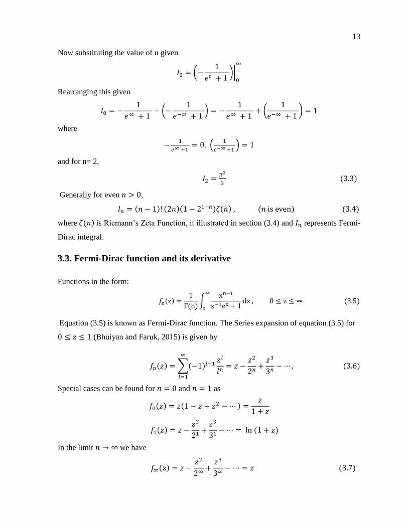
3.3. Fermi-Dirac function and its derivative

Functions in the form:

Equation (3.5) is known as Fermi-Dirac function. The Series expansion of equation (3.5) for

(Bhuiyan and Faruk, 2015) is given by

Special cases can be found for and as

In the limit we have

14

Recurrence relations:

For instance, using n values of half integral multiple (for fermions)

The asymptotic expansion for at low temperature is given by

3.4. Euler’s Gamma and Riemann’s Zeta functions

The Riemann’s Zeta Function is defined as a Dirichlet series (Boas and Stutz, 1971).

where =

.Using half integral multiple function of

=1.127

The Gamma Functions is defined for the complex z plane excluding the non positive integers:

For integer values the gamma function coincides with the factorial

function:

15

Some special values are

3.5. Expressions of internal energy and Equation of states of ideal gase

Internal energy of a system is the sum total energy of each particle in each particle energy

state. It can be express with partition function (Huang, 1987) as

The equation of states then takes in the form of the virial expansion (Tong, 2012) as

3.6. Expressions of Specific heat and entropy of ideal gas

The specific heat of ideal gas can be obtained by differentiating the internal energy with

respect to temperature, keeping total number of particles and volume constant (Pathria, 1996).

Thus,

And to examine the entropy of ideal gas system using thermodynamic formula from the

thermodynamic point of view, it is written as

And also the Helmholtz free energy can express in terms of entropy as

So that the entropy of ideal gas can be express in terms of Helmholtz free energy as

16

4. RESULTS AND DISCUSSION

4.1. Partition function of ideal Fermi-Gas

The grand canonical partition function applies to a grand canonical ensemble, in which the

system can exchange both heat and particles with the environment at fixed temperature,

volume, and chemical potential; it is the sum over all possible energy states that describe the

statistical properties of a system in thermodynamic equilibrium. It is a function of temperature

and other parameters, such as the volume enclosing the gas. Most of the aggregate

thermodynamic variables of the system, such as the total energy, free energy, entropy and

pressure, can be expressed in terms of the partition function or its derivatives. The sum of

partition function has a central role in statistical thermodynamics because once it is known as

a function of the variables on which it depends, all thermodynamic quantities may be

calculated from it directly.

Assume the energy of non interacting single-particle quantum state to be

the total energy of the system of identical particles is given as

where = is the number of particles in a single - particle state k. The total

number of particles of the system is therefore,

Then the grand-canonical partition function of an arbitrary non interacting Bose or Fermi

system is defined as

where

Now substitute Eq. and Eq. into Eq. , we get

17

Rearranging Eq. (4.5), gives

Thus, from Eq. (4.6) the grand canonical partition function for N indistinguishable fermions is

given by

The fermions have only two states, = 0 or 1. For =0 or 1,

Similarly for = 0 or 1,

Using these values in Eq. (4.7) yields

Equation (4.10) is the expression of the grand partition function of the system. Taking the

logarithm of the partition function

or

z is fugacity of the gas which is related to the chemical potential through . Using

this solution reshow Eq. (4.12) to the form

18

This is supposed to be Eq. given where the term appears in Eq. . In order to

express the partition function in the form of Fermi-Dirac function, consider a spin less ideal

Fermi gas confined in three dimensional box of side L is shown in Fig 3.

Figure 3: Three-dimensional box with volume V.

Then the energy can be express in the form of momentum as

The wave function is of the ideal Fermi gas is a solution of the Schrödinger equation

where is the Hamiltonian without the potential energy, in quantum theory, may

be represented by the operator

so that the ideal Fermi gas three

dimensional Schrödinger equations is

From our knowledge of quantum mechanics we expect the solution of this equation to be

represented by a standing wave, in three dimensions is

The have integer values the solutions vanish at and in the

wave vector as

19

where has components, thus

and

We can plot three vectors

in -space, where the points at the tips of the vectors fill the -space. These points are from a

cubic lattice with spacing

. The volume per point of -space is

. How many of the

allowed modes have wave vectors between and . are greater than zero

because negative k values do not add more energy states. Thus, if we imagine the set of points

at the tips of the wave vectors centered at the origin forming a sphere, we should take only the

positive octant. The number of modes with a wave vectors between and is

as shown in Fig 4. Then

Figure 4. Three dimensional systems of volume in k-space

where is the volume of the shell and

is volume per point and , then

Using where and considering that particles with momentum between and

20

On the other hand, the number of quantum states between momentums and is

where is linear momentum, is volume that is taken from momentum space. From

uncertainty principle we know that

Thus, is the length of the three dimensional box so that

, and

Then,

where is the volume of elementary cell in a phase space, and

and is volume and momentum space respectively. Now from the energy

we get momentum as

Thus,

where and are the mass and the linear momentum of a particle respectively, and energy

of states can also rewritten as,

This formula can also be derived by considering the classical phase space. Using Eq. (4.25),

(4.26), (4.27) and (4.28)

21

For three dimensional systems the sum converts to integrals and is the number of quantum

states lying between and or number of states in the one particle phase space. Then

the density of states for an ideal Fermi gas confined to a box of volume is defined as

To formulate the grand canonical partition function for a three dimensional ideal Fermi gases

substituting Eq. into Eq. as

Now to integrate Eq. we use the method of integration by parts

Let

Now substituting, Eqs. (4.34) and into Eq. , we get

From Eq. the term

since in Eq the first term of the product vanishes at upper limit and second term of the

limit vanishes at lower limit. The remaining term is

Let and

,

. Now Eq. (4.38) can be rewritten as

22

and

Taking out of the integral sign and expanding it in the form of gives

Let

where is the volume of phase space taken up by one state. Recalling Fermi-Dirac function

If

, the Fermi-Dirac functions written as

where

The integral of Eq. and Eq. are the same. Therefore,

Then the equations of state can be written in the form of partition function as

Rearranging Eq. gives

or

23

Using Eq. is can be written in the form of,

From the relations thermal de Broglie wave length

and

, the momentum of

particle can be related to its wave vector as = . Hence, the energy can be expressed in

the form of Eq. as

or

From,

Rearranging this yields

where =2 . Eq. (4.50) yields

Rearranging this gives

The relation between wave vector and the thermal de Broglie wave length can be expressed as

Here also the total number of particles can be obtained, from the grand canonical partition

function,

24

Substituting Eq. into Eq. we get

or

Using the recurrence relations:

Substituting Eq. (4.56) into Eq. (4.54) yields

Eq. is the total number of particles in the form of Fermi-Dirac function and when

written in the particle density form looks like

4.2. Internal energy of ideal Fermi-Gas

Internal energy of a system is the sum total energy of each particle in each particle energy

state. The energy levels are discrete. However, with many particles the energy levels will be

finely spaced and can be effectively treated as a continuum. The change in internal energy of

the Fermi gas must be positive, but a little below . As the temperature increases, more of the

low-lying states become vacant. To add a new particle without increasing the entropy, it

requires the new particle to go into a low-lying single-particle state, considerably well below

while once again cooling the gas slightly to avoid an increase in the number of microstates.

The total energy of ideal Fermi gas can be derived from grand canonical partition function as

25

Since

This gives

Substituting Eq. ( ) into Eq. gives

This implies

and substituting Eq. into Eq. yields

Differentiating this equation with respect to temperature gives

This implies that

Rearrangement of the above equation gives

Using with Eq. it is possible to reformulate Eq. as

Using Eq. as

26

Eq. yields

Again, we can now differentiate the grand partition function with respect to to check its

equality with Eq. . Similarly, we can substitute Eq. into Eq. gives

where

Inserting this into Eq. gives

In order to differentiate this with respect to we substitute

into Eq. . This

gives

Rearranging the equation gives

27

or

This can also be written by systematic rearrangement as

Substituting Eq. into this equation gives

Finally, the internal energy can be expressed in terms of Fermi functions as

such that the internal energy per particle becomes

From Eq. and

From Eq.

28

Rearranging this gives

And thermodynamic properties of ideal Fermi gas are conveniently expressed as functional

relations between variables known as equations of state. Using Eq. and Eq.

gives

Using Eq. we can write Eq. as

Then which implies that

or again, substituting Eq. into Eq. gives

so that Eq. is verified. From Eq. and

From Eq.

Replacing for in the above equation gives

Finally, the equation of state yields

The pressure of ideal Fermi gas also can be obtained directly from the logarithm of the grand

partition function as

29

so that this equation becomes

At higher temperature, for , or for small the Fermi-Dirac function

can be expanded as a convergent series such that

which is derived in Appendix A. When

the above equation becomes

when,

Since we can do the following approximation for the two functions:

Hence, by using the above expansion into Eq. the equation of state becomes:

so that is determined by density of particles and it is in the form of the series expansion of

the Fermi-Dirac function (Eq. 4.58)

From Eq. and Eq. , we can get

This is identical to the equation of state of a classical ideal gas. From the relationship

30

At , (and hence , both pressure and specific heat of the gas approach their

classical values, known by

and

respectively. Also, in the series expansion for

and

only the first two terms can be retained as,

Thus, Eq. and Eq. can be reduce as

and

or

The simplest approximation in this limit is

This is equivalent to assuming that

, that measures the particle density and the thermal

de Broglie wave length are small and since

, the temperature is high. In the next

approximation using the notation

Starting from the binomial series

31

Hence, when

The equation of state for pressure is then

or

Factoring out gives

Then substituting

(Eq. ) we obtain

or

Multiplying both sides of the above equation by

yields

Therefore, the equation of state in the first quantum correction can be

From Eq.

32

Substituting for from Eq. gives

Then the internal energy per particle gives as

In this expression, the first term corresponds to the internal energy for the classical ideal gas,

while the second term is the first quantum mechanical correction.

For temperatures much larger than the Fermi temperature, , the Fermi-Dirac

distribution approaches to Maxwell-Boltzmann, and the equation of state tends towards that of

the ideal classical gas as

The equation of state then takes in the form of the virial expansion such that Eq. can

be extended to higher order and it can be

The explicit form of Eq. (4.99) is

where, are the virial coefficients of expansion of the pressure, with values

,

and so on. This derivation shown under Appendix C. This

expansion is valid when is small, which means low density and high temperatures. Eq.

(4.100) can also be rewritten as

Then the relation between internal energy and the equation of state (Eq. (4.76) and Eq. (4.85)

can be gained to give

33

Inserting Eq. into Eq. ), the internal energy of ideal Fermi-gas equates

At high temperature , we can consider two cases to express the thermodynamic

properties of ideal Fermi gases in terms of temperature parameters.

Case : In the limit goes to one , the Bose gas in the infinite series can be

expressed as Riemann’s Zeta Function as

If we set alpha =

we obtain

and

But in the case of Fermi gas at , we need an extra effort to get the corresponding

integral, so that the infinite series can be expressed as Riemann’s Zeta Functions as

If

Thus, in general for

34

In terms of Riemann zeta function this can rewritten as

and if

so that

Hence, the total number of particles at can be expressed as Riemann’s Zeta Functions

as

which is derived below in the appendix B and this implies that at , and

because we consider the range of fugacity, so at the fugacity

or

becomes which means and which is the quantum

effects of the system so that the temperature of the system is Fermi temperature but when

from absolute zero temperature then or

is approaches to zero which is the

classical effect so that the temperature of the system is normal temperature then the above

equation becomes

Substituting this equation into Eq. we get

Thus,

This is the internal energy per particle at a higher temperature, where

, and so on.

35

The behavior of the Fermi gas at low temperatures is very different than that of the Bose or

the classical gas, due to the fact that the maximum number of particles that can occupy an

energy level is one for Fermions. As particles are added into the box they must occupy higher

and higher energy levels, so that the last particles to be added are in states with high kinetic

energy. Even at low temperatures the Fermi gas then has a high pressure, called the

degeneracy pressure, and the particles have high kinetic energy.

To understand the degeneracy pressure and other properties of ideal Fermi gases, we first

need to understand the chemical potential and the fugacity at low temperatures. Since at low

temperatures the chemical potential is controlled by the energy contribution, and the energy

required for adding a particle to the volume is equal to the lowest unoccupied single particle

energy level, the chemical potential is finite and positive at low temperatures. In that case,

becomes large at low temperature and the fugacity is then very large and positive.

In the low temperature limit the Fermi distribution function behaves like a step

function. This means, all the states with energy below the Fermi energy ,

are occupied and all those above are empty. In momentum space the occupied states lie within

the Fermi sphere of radius . Such situation is quantum degeneracy. For mathematical

convenience we approximate the discrete energy levels by a continuum, which is valid

provided there are a large number of accessible energy levels. Replacing the level variables

with continuous quantities ( and , the number of particles at

energy is written,

where is the density of states. The total number of particles (N) and total internal energy

(U) follow as the integrals respectively,

The density of states is defined such that the total number of possible states in phase

space is,

36

Figure 5: The volume of momentum space from p to dp in 3D momentum space.

In Fig 5, the quantity represents the number of states lying between momentum

and . These states occupy a volume in phase space which is the sum of their

volume in position space and their volume in momentum space. The box volume and

the range and represents a spherical shell in momentum space with inner radius

and thickness with momentum space volume . Hence the phase space volume

is . Now recall that each quantum state takes up a volume in phase space. Thus

the number of states between and

From Eq. (4.28) is given as

This is the density of states for an ideal gas confined to a box of volume. These are

diminishing amount of states in the limit of zero energy and increasing amount with large

energy. At , all states are occupied up to and with this simplified distribution it is

straight forward to integrate the number of particles,

Now substituting for from Eq. into this equation gives

37

Substituting for from Eq. (4.113) and assuming gives

Hence

In order to obtain the total number of particles at ground state the above equation has to be

integrated to yield

Rearranging this equation given the Fermi energy in terms of particle density

or

with a corresponding Fermi temperature

Alternatively, the Fermi energy can be expressed in Fermi momentum and Fermi wave

number.

Figure 6: Fermi surface in momentum space

38

As shown in Fig 6, at absolute zero temperature, all states within the Fermi sphere in

momentum space are occupied and the rest are empty. The radius of the sphere is the Fermi

momentum , where is the Fermi wave vector. Using the momentum space

The Fermi surface is described by and Equating Eq. and Eq. gives

the Fermi wave number

Rearranging this equation we obtain the particle density as

At the system is in its ground state, with the internal energy given by

Substituting for from Eq. (4.108)

Replacing from Eq. (4.113) results in

After integrating the above equation the ground state internal energy is obtained and it is

Expressing Eq. and Eq. in terms of and equating

Rearranging and cancelling like terms yields

39

This equation, shows quantum effect because, classically the total internal energy of the

system at absolute is zero. Hence the internal energy per particle at absolute zero temperature

is

This indicates that even at ground state, the internal energy of the Fermi gas is positive. This

is due to the fact that only one Fermion can be in each energy level, which means high energy

states are occupied at absolute zero temperature. As the density increases the Fermi energy or

energy of the highest occupied states increases. The ground state energy is clearly a quantum

effect arising due to Pauli Exclusion Principle due to which the system cannot settle down

into a single energy state as in the case of Bose gas and it is directly proportional to the total

number of particles and the Fermi temperature. And therefore, some particles are spread over

a lowest available energy states even at absolute zero temperature in lots of kinetic energy;

classically the total energy of a system at absolute zero temperature is zero.. Since

the pressure, is

Replacing Eq. , gives

or

where is number of particle per volume as

Replacing Eq. in Eq. its equivalent value in Eq.(4. 117) yields

40

Thus the ground-state pressure of an ideal Fermi gas at absolute zero temperature solely

depends on its concentration

. This zero-point pressure arises from the fact that there must

be moving particles at absolute zero temperature since the zero momentum state can hold only

one particle of a given state and the pressure increases with density. The ground state pressure

is a quantum effect arising due to Pauli Exclusion Principle; even at absolute zero temperature

the particles move inside a cubical box and hit the well of the box then produce the ground

state pressure.

Case : Quantum limit ( From Eq. we recall that the Fermi energy

at is

From this relation, the Fermi temperature can be expressed in terms of particle density as

Dividing both sides of the equation by gives

Expressing as

transforms the equation to

The equation can rewritten as

or

Rearranging this gives

41

Then dividing both sides by yields

Since

Rearranging this equation gives

Now substituting Eq. into Eq. , we get

Next substituting the virial coefficients,

, so on, we get

or

Recalling Eq.

, the equation of state,

42

At high temperatures Fermi gases act like a classical gases. The chemical potential is the

energy necessary to add one particle to the system without changing both the entropy and

volume and it is given by,

Now using Eq. into we obtain

or

Then using the properties of logarithm (i.e.)

the above equation becomes

which is the chemical potential at higher temperature and it is negative.

For low temperature the Fermi-distribution deviates from that at mainly in the

neighborhood of in layer of thickness particles of energies of the order of below

the Fermi energy are excited to energies of the order of above the Fermi energy. In the

low temperature limit, , a fixed density corresponds to the condition

In the low temperature limit, is large and one cannot use power series expansion for

deriving an asymptotic formula for

and

. Instead, such formula is obtained by the

asymptotic expansion as

43

This expansion is derived in Appendix A. Hence, if

the above equation becomes

Then, we get

Retaining the first term of the given result of

where

Rearranging Eq. (4.137) gives

At ,

,

and Eq. gives

which gives the correct limiting value for the chemical potential including the next order in

the expression of Eq. ,

This can be rewritten as

We now substitute on the right-hand side of this equation by

( Eq. 4.139)

44

Using the series expansion

and considering the first two terms

From Eq. (4.139) and Eq. follows the asymptotic formula for the chemical potential:

Hence

Multiplying both sides by

the chemical potential gives

This equation can be rewritten as

Moreover, the above equation written in the second order series expansion as

Then we can write the chemical potential in terms of different values of temperatures

At low temperature we use the asymptotic expansion to expand the Fermi Dirac function to

express the thermodynamic properties of ideal Fermi gas in terms of the expansion of the

Fermi Dirac function and it is written as

45

which, if

gives

so that after some rearrangement this written as

If

following the same procedure

and if

Recalling that

Eq. transform to

or

where

Hence, the particle density is

or

46

In the zero approximation

Eq. is identical with the ground state result . In the next approximation, we

obtained

In order to get the internal energy of ideal Fermi gases, substituting Eq and Eq.

into gives

Then after some rearrangement we can write

The above equation is simplified as

Applying the binomial series

Dividing both sides by gives

Linking this with Eq gives

Then after multiplying and some rearrangement the above equation can be written as

47

or

where

so that adding the above terms becomes

This is the first order series expansion of the internal energy per particle. This equation can be

written in the second order series expansion as

or

The pressure of the ideal Fermi gas is then given as

and the equation of state is,

or

Thus, the equation of state can be written as

48

Therefore, the total internal energy, pressure and the equation of state of the ideal Fermi gas

are expanded in terms of even number power of temperature parameters at low temperature.

The internal energy of ideal Fermi gas can be written in different values of temperature as

4.3. Specific heat of ideal Fermi-Gas in normal phases

The importance of the heat capacity is defined in terms of things that we can actually measure

and it is always proportional to the number of particles in the system. In three dimensional

Fermi-gases, contribution to heat capacity comes from the states on Fermi surface. The

specific heat of the ideal Fermi gas can be obtained by differentiating the internal energy with

respect to temperature, keeping total number of particles and volume constant, and follows the

recurrence formula. From Eq. (4.84) and Eq. (4.85)

or

Since from Eq. (4.77)

Inserting this into Eq. (4.162) yields

49

In order to evaluate the differentiation with respect to temperature we have to employ the

product rule which gives

Next applying the quotient rule on the last term of the above equation

Using chain rule,

Using the recurrence relation

From Eq. (4.137a)

Since from Eq. (4.41)

Substituting this into Eq. (4.168) gives

50

Multiplying the right hand side by

gives

Thus,

Eq. can also be rewritten in the form

and using the recurrence relation

Equating Eq. ( with Eq. gives

Similarly equating Eq. with Eq. gives

This implies

where

51

Dividing both sides of Eq. by

yields

Using Eq. and Eq. in Eq. gives

Then substituting for

from Eq. in Eq. we get

or

Further simplification gives

or

Then the specific heat capacity of ideal Fermi-gas at higher temperature is

The classical limit at high temperature can easily be obtained taken from the

above equation, by considering

52

Hence

that gives

Starting with Eq. (4.162) and replacing U from Eq. (4.97) gives

Then

After differentiating we get

or

After rearrangement this equation becomes

Therefore the specific heat per particle of the ideal Fermi gas at high temperature can be

written as

53

Recalling case at and substituting Eq. in Eq. (4. 183) gives

After some rearrangement this becomes

In order to get the higher order heat capacity of the ideal Fermi gas at we used Eq.

as a function of temperature parameter

. Eq. is the most general, written

in terms of fugacity ( . Eq. can be evaluated in terms of temperature parameters using

the relationship

Recalling equation of pressure given by

where is determined by implicit relationship

and

Now we can eliminate the fugacity z using

54

Rearranging Eq. we obtain as

where virial coefficients and their values are given as

, so on. Now substituting the value of the virial

coeffietients into the above equation we get

Using Eq. into Eq. (i.e. replacing

) gives

or

which is the specific heat at higher temperature at and at Substituting

Eq into Eq. gives

Thus,

To obtain the higher order quantum correction we can differentiate Eq. with respect

to temperature as

This implies

55

Thus, at a finite temperature, the specific heat of the gas is smaller than its limiting value,

. The heat capacity of an ideal Fermi gas is the energy required to raise its temperature

by unit amount at a constant volume. From the temperature dependent part of the total energy

or Eq. we obtain specific heat of the gas at a constant volume for low temperature.

Substitute Eq. into Eq. gives

Finally, the equation simplifies to

Replacing for gives

Eq. is the series expansion of specific heat of ideal Fermi gas at low temperature and

it is valid for , and . It shows that at a temperature much less than the Fermi

temperature, the heat capacity is proportional to the temperature, and vanishes in the

limit . Thus, for ,

is the Fermi temperature of the system and since the

Fermi temperature is proportional to the two-third power of density and hence a high density,

Fermi density gas has a high Fermi temperature. The Fermi gas is called degenerate if its

temperature is much lower than Fermi temperature. The specific heat varies linearly with

temperature; moreover, in magnitude, it is considerably smaller than the classical value. Since

56

the specific heat per particle of ideal Fermi gas can be expressed in terms of different values

of temperature as

4.4. Entropy of ideal Fermi-Gas

Entropy is the measure of randomness in a system and it depends only on the state of the

system. In this section, we have to examine the entropy of ideal Fermi gas system using

thermodynamic formula. From the thermodynamic point of view it is written as

Dividing both sides by gives

The Helmholtz free energy of the gas is given as

From Eq.

Now replacing for in Eq. (4.203) gives

Using the relation

the equation can also be written as

Using quantum statistics, fugacity is expressed as

57

That means,

or

Substituting Eq. into Eq. gives

or

which is the Helmholtz free energy in terms of Fermi-Dirac function. The entropy of the ideal

Fermi gas can be expressed in terms of internal energy and Helmholtz free energy as

Substituting Eq. and Eq. into Eq. yields

or

Now collecting like terms we obtain

58

or

This is the expression of entropy per particle at a higher temperature limit. Now using Eq.

and Eq. a result the form

Writing the summation in expand form gives

Using the values of the virial coefficients,

and

etc the sum becomes

At , substituting Eq. into Eq. we obtain

Then after some rearrangement we get

This is called the entropy per particle at higher temperature, and using Eq. into

Eq. we obtain

so that at , hence this equation can be written as

59

This is called the entropy per particle of gas in terms of temperature parameter at higher

temperature. For low temperature, limit, the Helmholtz free energy of the system

follows direct substitution of Eq. and Eq. into Eq.

or

and then by subtract like terms the above equation simplify as

so that the Helmholtz free energy of ideal Fermi gas in terms of temperature parameter is

written as

from which the Helmholtz free energy per particle at low temperature is given as

Noting that ,

The entropy of ideal Fermi gas can be obtained from Helmholtz free energy at low

temperature as

60

Substituting Eq. into Eq. we get

The entropy of ideal Fermi gas can be written in terms of temperature parameter at low

temperature is

At since the entropy has no contribution in the absolute zero temperature

limits. Hence, the Helmholtz free energy and the entropy of ideal Fermi gas can be expanded

at low temperature in terms of even and odd number power of temperature parameters

respectively. Now we can write the entropy per particle of ideal Fermi gas at different values

of temperatures as

4.5. Numerical results

In this section, the numerical results of the macroscopic properties of the ideal Fermi gas are

presented and discussed. In order to perform the numerical analysis of the chemical potential,

internal energy per particle, specific heat per particle, equation of state per particle and

entropy per particle are first converted into matlab source code. Eqs.

, , and where used to obtain the figures ( Fig 6-Fig 10).

61

4.5.1. Chemical potential

The chemical potential for ideal Fermi gas is given in Eq. This result allows us to

plot the chemical potential as a function of temperature. For the sake of convenience, both

axes where made to be dimension-less such that the study will not become system-specific.

Figure 6 displays chemical potential as a function of temperature parameter.

Figure 7. Chemical potential of ideal Fermi gas versus temperature parameter

Figure 6 illustrates the numerical results for chemical potential of ideal Fermi gas below and

above Fermi temperature . This particular result is obtained by taking the range of the

temperature parameter (

). Moreover, the chemical potential is defined as the

Fermi energy at , vanishes at Fermi temperature. From Figure 6 we see that the

chemical potential decreases from Fermi energy at , which is quantum behavior to

smaller and smaller values, until . At all low lying single particle states are filled,

up to Fermi energy in accordance with Pauli Exclusion Principle. All states above Fermi level

are empty. There is only one microstate available to the system. When adding another

Fermion, at , it must going to a single particle state just above the Fermi level. So the

energy increase of the system is and thus . Note that this is a positive

quantity, so there is still only one available microstate. As the temperature rises, the total

internal energy of the system increases, and some fermions begin to occupy excited states. If

62

the gas is at very low but non zero temperature and consider the effect of adding one particle,

the entropy of the system must not increase when the particle is added. The new particle must

going to one of the states close to the energy level , since fermions leave these states first

when excited higher states. In fact, the new particle must be going to a low lying vacant single

particle state which will be a little below the gas must also be cooled a little to avoid

increasing the number of accessible microstates. Usually, adding a particle to a system causes

an increase in the number of accessible microstates, even if the internal energy of the system

remains constant. The reason is the number of ways of distributing the total energy among the

particles is increase. The change internal energy of the Fermi gas, must be positive

but a little smaller than until , just below the , at which even the single particle

ground state is unlikely to be occupied.

After this point, as the temperature rises, the gas eventually begins to mimic classical

behavior and the chemical potential decreases and becomes increasingly negative. If a new

particle is added to the system the internal energy must decrease, the entropy remains

constant. The chemical potential measures the change in internal energy of the system when

one more particle is added, while holding the volume and the entropy constant, adding the

particle while allowing the internal energy of the system to decrease by . This makes the

total energy Thus the entropy remains constant, so and this

negative sign simply indicates that the system’s energy must decrease as a particle is added.

At both classical and quantum effects of the chemical potential are unrealistic, even

at , the discontinuity shows, the transition region which signifies to separate classical

and quantum regions.

4.5.2. Internal energy

The internal energy per particle for ideal Fermi gas is given in Eq. (4. 161). Figure 7 displays

this result as a function of temperature above and below the Fermi-temperature.

63

Figure 8. Internal energy of ideal Fermi gas versus temperature parameter

Figure 7 illustrates the numerical results for the internal energy of ideal Fermi gas by taking

the range of the temperature parameter (

). In the high temperature limit ( ,

the internal energy of free quantum gases reduces to the form of classical gas. At T = 0, the

internal energy of the classical gases goes to zero. In low temperature limit ( the

internal energy of the quantum gas of fermions never goes to zero. It suggests that the non

zero ground state energy seen here is clearly a quantum effect arising due to the Pauli

Exclusion Principle. This shows that the internal energy of the Fermi gas is positive, and only

one Fermion can be in each energy level so high energy states are occupied even at zero

temperature. As the density increases, the Fermi energy or energy of the highest occupied

state increases, this is the quantum behavior of the gas. At T = 0, the system is in its ground

state, and the particles are distributed among the single particle states so that the total energy

of the gas is at minimum. As the temperature raise, the total internal energy of the system

increases and the gas tends to manifest classical behavior, that is, it only shows linear

dependence on temperature. When , both classical and quantum effects of the internal

energy are unrealistic, even at , the discontinuity shows the transition region, which

signifies to separate classical and quantum regions.

64

4.5.3. Equation of state

The equation of state for ideal Fermi gas above and below the Fermi-temperature is given in

Eq. (4.160). Figure 8 displays this result as a function of temperature

.

Figure 9. Equation of state of ideal Fermi gas versus temperature parameter

Figure 8 illustrates the numerical results for equation of state of the ideal Fermi gas below and

above Fermi temperature. This particular result is obtained by taking the range of the

temperature parameter

). Figure 8 shows that in classical limit, at higher

temperature the equation of state is linear in temperature so that the pressure of the

gas increase with temperature, but at zero temperature it goes to zero. In quantum limit, at

lower temperature the ground state pressure never goes to zero. It suggests that the

ground state pressure seen here is clearly a quantum effect arising due to the Pauli Exclusion

Principle, which allows only one particle to have zero momentum, but all other particles have

finite momentum. Figures 7 and 8 appear to display similar shape, but with slight difference

in magnitude by a factor of

near absolute zero. At the pressure is unrealistic because

our estimation of thermodynamic properties of ideal Fermi gas is at lower and

higher temperature. When both classical and quantum effects of the

65

equations of state are unrealistic, even at , the discontinuity shows the transition

region, which signifies to separate classical and quantum regions.

4.5.4. Specific heat

The specific heat for ideal Fermi gas above and below the Fermi-temperature is given in Eq.

(4.205). Figure 8 displays this result as a function of temperature.

Figure 10. Specific heat of ideal Fermi gas versus temperature parameter

Figure 9 illustrates the numerical results for specific heat of ideal Fermi gas as a function of

temperature parameter. This particular result is obtained by taking the range of the

temperature parameter (

). In the higher temperature limit, the limit of specific heat

approaches its classical value as it becomes

. This is constant, independent of

temperature, in violation of the third law of thermodynamics. This is because of the classical

approximation, even at zero temperature it is different from zero. Instead, at low temperature,

due to quantum correction it gradually reduces and we typically find a very small contribution

to the heat capacity which is linear in temperature, a result that can be explained by quantum

mechanics. At zero temperature it goes to zero according to third law of thermodynamics

which is the consequence of quantum mechanics and becomes lower and lower at low

66

temperature. For a small increase in temperature, only Fermions close to the Fermi energy are

excited. Most of the Fermions are below the Fermi energy and are not excited at all. Since

they cannot be excited, these Fermions would not contribute to the heat capacity. So it is

mainly the fermions close to the Fermi energy that would contribute to the heat capacity. So

we used these to estimate the heat capacity and ignored the rest at which is unrealistic

specific heat. At both classical and quantum effects are unrealistic, even at the

discontinuity of the graph shows the transition region, which signifies to separate classical

and quantum regions. When and quantum and classical effects are display

respectively.

4.5.5. Entropy

The entropy for ideal Fermi gas above and below the Fermi-temperature is given in Eq.

(4.226). Figure 8 displays this result as a function of temperature.

Figure 11. Entropy of ideal Fermi gas versus temperature parameter

Figure 10 illustrates the numerical results for entropy of ideal Fermi gas as a function of

temperature parameter. This particular result is obtained by taking the range of the

temperature parameter (

). In classical limit, at higher temperature, the entropy of

the classical ideal gas is constant in temperature; even at it is different from zero. In

67

quantum limit, at lower temperature, the entropy will gradually reduces, even at zero

temperature it goes to zero, which means the fermions are well ordered which is the quantum

effect of the gas. The entropy is reduced at low temperature because a nearly degenerate

Fermi gas is highly ordered; permutation symmetry strongly reduces the number of states

available to fermions. At , the values of entropy is negative. This is totally unrealistic

and it is in violation of the third law of thermodynamics, because our estimation of

thermodynamic properties of ideal Fermi gas is at lowers temperature and higher

temperature . At both classical and quantum effects are unrealistic, even at

the discontinuity shows the transition region, which is signifies to separate classical

and quantum regions.

68

5. SUMMARY, CONCLUSION AND RECOMMENDATIONS

5.1. Summary

In the present study, the grand partition function, the chemical potential, internal energy,

equation of state, specific heat and entropy of the non interacting Fermi gas are calculated in

the framework of Fermi Dirac function. Approximation forms of thermodynamic properties of

ideal Fermi gas were obtained for lower temperature using asymptotic expansion of Fermi-

Dirac function and for higher temperature using the virial expansion method and series

expansion of Fermi Dirac function.

The numerical analysis of thermodynamic properties of an ideal Fermi gas performed using

Matlab program language to generate plots of our calculations for higher and lower

temperature limit. For numerical analysis we have used fifty data points (N=50) to present the

numerical results for the thermodynamic properties of ideal Fermi gas at lower and higher

temperatures. Comparison of these quantities in the numerical and series expansion methods

shows a good agreement with their theoretical description at lower and higher temperatures.

At absolute zero temperature the specific heat and entropy of the ideal Femi gases have no

value and the internal energy of the Fermi gas is positive which means only one Fermion can

be in each energy level such that further energy states are also occupied. The ground-state

pressure of an ideal Fermi gas at absolute zero temperature solely depends on its

concentration and there must be moving particles at absolute zero temperature since the zero

momentum state can hold only one particle of a given state and the pressure increases with

density. At higher temperature, the internal energy and equation of state of the non interacting

Fermi gas increase and decrease at low temperature, but the specific heat and entropy of ideal

Fermi gas are constant at higher temperature and gradually reduces at lower temperature. The

chemical potential is negative at higher temperature which is classical effect. For temperature

near the Fermi temperature, the values of the thermodynamic properties of ideal Fermi gas is

un-physical because our estimation at lowers temperature and higher

temperature .

69

5.2. Conclusion

In the present study, we have introduced the basic concept of the basic macroscopic properties

of ideal Fermi gas through the application of quantum mechanics. We have also studied

relationship of these parameters with Fermi temperature and the normal temperature .

We have demonstrated the thermodynamic properties of the ideal Fermi gas through the

application of quantum mechanics. The greatest success of this study is to explain the

thermodynamic properties of the ideal Fermi gas in the lower temperature limit through the

application of quantum mechanics.

At absolute zero temperature, the chemical potential of ideal Fermi gas is equal to the Fermi

energy, and as the temperature continues to rise; the chemical potential decreases and

becomes increasingly negative and eventually begins to mimic classical behavior. This

decreasing chemical potential indicates that particles move from energy states below the

Fermi energy to energy states above the Fermi energy. The internal energy of the ideal Fermi

gas at absolute zero temperature leads to the nonzero ground state energy which is clearly a

quantum effect arising due to the Pauli Exclusion Principle. This shows that the internal

energy of the Fermi gas is positive, and only one Fermion can be in each energy level so high

energy states are occupied at absolute zero temperature. As the temperature rises, the total

internal energy of the system increases and some of the fermions begin to occupy excited

states.

The ground state pressure is clearly a quantum effect arising due to the Pauli Exclusion

Principle, which indicates that at absolute zero temperature, particles move around, hit the

wall of the cubic box and exert pressure. As the temperature rises, the pressure increase,

which means, it has linear dependence on temperature. At low temperature limit, both specific

heat and entropy of the ideal Fermi gas have the same numerical value, and at absolute zero

temperature both specific heat and entropy gets zero according to the third law of

thermodynamics which is the consequence of quantum mechanics. As the temperature gets

higher, the value of both specific heat and entropy of the ideal Fermi gas almost constant

which means they are independent of temperature, so that the gas is called classical gas. For

the near temperature the Fermi temperature, the values of the macroscopic properties of the

70

ideal Fermi gas are unrealistic because we used the approximations, at lowers and

higher temperature to performed calculations.

5.3. Recommendations

In the present study the thermodynamic properties of an ideal Fermi gas confined in cubical

box volume have been studied conventionally in thermodynamic limit by ignoring the

interaction between particles in the gas through the application of quantum mechanics. For

realistic study, interactions between constituents of the Fermi gas should be included.

Moreover, a follow up study of the thermodynamic properties of interacting Fermi gas can be

carried out through the application of the laws of quantum mechanics and the mean field

approximation.

71

6. REFERENCES

Bagnato, S. and Rochin, R. 2005. Thermodynamics of an Ideal Gas of Bosons Harmonically

Trapped: Equation of State and Susceptibilities. Brazilian Journal of Physics,

35(3A): 607-614.

Bhuiyan, G. and Faruk, M. 2015. Thermodynamics of ideal Fermi gas under generic power

law potential in d-dimension. Journal of acta physica polonika B, 46(12): 2419-2434.

Boas, R. and Stutz, C. 1971. Estimating sums with integrals. American Journal physics, 39:

745.

Cook, G. and Dickerson, R. 1995. Understanding the Chemical Potential. American Journal

physics, 63(8): 737-774.

Cornell, E. 1996. The Nanokelvin physics of Bose-Einstein Condensation. National Institute

of Standards and Technology and University of Colorado. Journal of Research of the

National Institute of Standards and Technology, 101(4): 419-434.

Cowan, B. 2019. On the Chemical Potential of Ideal Fermi and Bose Gases. Journal of Low

Temperature Physics, 197: 412-444.

Dirac, P. 1926. On the Theory of quantum Mechanics. Proceedings of the Royal Society,

London, A (112): 661.

Dorlas, T. 1999. Statistical Mechanics Fundamental and Model solutions. IOP Ltd. pp. 128-

222.

Fenech, K., Dyke, P., Peppler, T., Lingham, M., Hoinka, S., Hu, H. and Vale, C. 2016.

Thermodynamics of an Attractive 2D Fermi Gas. Physical Review Letters, 116:

045302.

Fermi, E. 1926. On the quantization of the mono atomic ideal gas, Journal of Rendiconti

Accademia Lincei, 3: 145.

Ghosh, S. and Padhi, B. 2013. Cavity optomechanics with synthetic landau levels of ultra

cold Fermi gas. Physical Review Letters, 111: 043603-043642.

72

Hang T., Anh, T., Dien, V., Van, T., Lan, T. and Viet, A. 2014. Thermodynamic equivalent

between non-interacting Bose and Fermi gas in metallic carbon nano tubes.

Communications in Physics, 24(3S2): 146-150.

Huang, K. 1987. Statistical Mechanics, Second edition. Massachusetts Institute of

Technology, John Wiley & sons. pp. 127-243.

Jaffe, L. 1996. Degenerate fermions systems Lecture note, 8.322. Massachusetts Institute of

Technology, Cambridge. 3p.

Kelly, J. 1996. Statistical Mechanics of ideal Fermi systems. Universidad Autonoma de

Madrid. Retrieved 2018-03-15. Ideal quantum Gases: Statistical physics using

Mathematica. 14p.

Landau, L. and Lifshitz, E. 1970. Statistical physics. Butterworth-Heinemann, University of

Oxford, England. 5: 544.

Leggett, A. 2006. Quantum Liquids, Bose condensation & cooper pairing in condensed matter

systems, Oxford University press. 34p.

Luo, L. 2008. Entropy and Super fluid Critical Parameters of a strongly interacting Fermi gas.

Doctoral Dissertation, University of Duke, Durham, North Carolina. pp. 2-3.

Maxwell, J. 1860. Illustrations of the dynamical theory of gases. Part I. On the motions and

collisions of perfectly elastic spheres, Philosophical magazine. 4th

series. 19: 19-32.

And Part II. On the process of diffusion of two or more kinds of moving particles

among one another, Philosophical magazine, 4th

series. 20: 21-37.

Mullin, W. and Blaylock, G. 2003. Quantum statistics. University of Massachusetts,

Amherst. American Journal physics, 71(12): 1223.

Mullin, J. and Fernandez, P. 2002. Bose-Einstein Condensation, Fluctuations, and Recurrence

Relations in statistical Mechanics. University of Massachusetts, Amherst,

Massachusetts01003. arXiV: cond-mai/0211115v3 [cond-mat.stat-mech]. 10p.

73

Obregón, O. and Cruz, M. 2017. Generalized Entropies Depending Only on the Probability

and their Quantum Statistics. 4th

international Electronic conferences on entropy and

its application. Proceedings 2018. 169: 2.

Pathria, R. 1996. Statistical Mechanics, Second edition, University of Waterloo, Waterloo,

Ontario, Canada. pp. 158-166.

Pathria, R. 1998. Similarities and differences between Bose and Fermi gases. Physical

Review, E 57: 2697-2702.

Pathria, R. and Beale, P. 2011. Statistical Mechanics, Third edition. Journal of contemporary

physics, 52: 619-620.

Pauli, W.1925. On the connection of the conclusion of the electron groups in the atom with the

complex structure of the spectra. Journal for physics, 31: 765-783.

Pauli, W. 1940. The connection between Spin and Statistics. Physical Review, 58: 716.

Pearson, J. 2008. Thermal physics of Bose and Fermi gases, University of Manchester. 10p.

Pelster, A. and Klǜnder, B. 2009. Systematic semi classical expansion for harmonically

trapped ideal Bose gases. European Physical Journal, B68: 457-465.

Pethick, C. 2008. Bose-Einstein Condensation in dilute gases, Second Edition, Cambridge

University press. pp. 1-5.

Sanner, C., Su, E., Keshet, A., Gommers, R., Shin, Y., Huang, W. and Ketterle, W. 2010.

Suppression of Density Fluctuations in a Quantum Degenerate Fermi Gas. Physical

Review Letter, 105 (4): 040402.

Santra, B. 2014. Thermodynamics and statistical mechanics, Indian Institute of Technology

Guwahati-781039, Assam, India. 69p.

Sevilla, F. 2011.Revisiting the concept of chemical potential in classical and quantum

gases: A perspective from Equilibrium Statistical Mechanics. arXiV: 1104.2611V1

[cond- mat.stat.mech]. 12p.

74

Sevilla, F. 2016. Thermodynamics of low-dimensional trapped Fermi-gas. Journal of low

temperature physics, 175: 427-434.

Soroka, A. and Poluektov, Y. 2017. Thermodynamics of the Fermi gas in a nano tube.

arXiV: 1704.03317V1, physics.gen-ph. 56p.

Swendsen, R. 2002. Statistical mechanics of classical systems of distinguishable particles.

Journal of Statistical Physics, 107: 1143-1165.

Tong, D. 2012. Statistical physics part II mathematical tripos, University of Cambridge, UK.

pp. 62-63.

Tora, R. and Peralta, A. 2016. Ensemble Equivalence for Distinguishable Particles. Entropy,

18: 259-272.

Vignolo, P., Minguzzi, A. and Tosi, M. 2000. Exact Particle and Kinetic-Energy Densities

for One-Dimensional Confined Gases of Non interacting Fermions. Physical Review

Letter, 85: 2850.

75

7. APPENDICES

Appendix A: Fermi-Dirac function

In this section, the series expansion of the Fermi-Dirac function,

is derived clearly at higher temperature and also we derive the asymptotic expansion at low

temperature. We first investigate the properties of the Fermi-Dirac function for

we may denote a series expansion

Then substitute this equation into Eq. , gives

This equation is the series expansion of the Fermi-Dirac function at high temperature.

Where

Moreover, to derive the series expansion of the Fermi-Dirac equation at low temperature we

start from the logarithm of the grand partition function:

76

And the wave vector is defined as

Each state has in k-space an average of

In the thermodynamic limit, when , and

constant, so that the

sum can be substituted by an integral over space as

Now substituting, Eq. into Eq. we obtain

In terms of spherical coordinates we have

Let

,

and

Then,

But already we derived in the above the grand partition function in terms of Fermi-Dirac

function as

77

Now we consider Eq. and Eq. gives

And

In order to calculate the integral, we perform aTaylor expansion of the logarithm:

So that Eq. can be expand as

Substitute Eq. into Eq. gives

Which is the series expansion of the Fermi-Dirac function at higher temperature (

Now also apply Eq. one can we get

78

This series expansions, for

and

are poorly convergent at low temperature, so we

need a different approach. Following the asymptotic expansion, it is more convenient to carry

out an expansion in . The procedure is as follows, we work the integral form

of

. We change variables to , then and integrate by parts,

Substitute Eq. into Eq. , we obtain

And then

Now substitute Eq. into Eq. we get

By using integration by parts we can integrate Eq. :

Let

,

(19A)

And

Then substitute Eq. (18A) into Eq. we get

79

But,

And

Then consider Eq. , we get

Or

The integration by parts leads to an integrand that is convergent at large . Now we expand

in a Taylor series about ,

So that, substitute Eq. into Eq. , we get

Defining yields

Now we break the integral up as

80

From the above equation the second integral is exponentially small, O , so we can ignore

it. Finally we have,

Where

, while by symmetry is zero for odd . For even is related to the Reimann

zeta function, through,

If ,

Substitute Eq. into Eq. and employing Eq. we get

Then, this equation can be simplify as

So that we can write in a general form as

Or

81

This is the series expansion of the Fermi-Dirac expansion at lower temperatures

82

Appendix B: Integrals in quantum statistics

In quantum statics we frequently encounter integrals of the form:

Where the plus sign is for Fermi statics and minus sign for Bose statics, and is appositive

number, usually an integer, or a half-integer. Since for , we may substitute the

following expansion,

Now substitute this equation into Eq. and integrate it term by term. If , we have

For the Bose case the infinite series can be expressed as a Riemann zeta function

with . In general is defined as

With appositive number, in fact it is required that otherwise the series diverges.

We need an extra effort to get the corresponding integral for Fermi statistics,

83

Or

By using the same approach, one can evaluate the following two types of integrals (for

positive ):

This is for the Bose case, but for the case of Fermi statistics

For a degenerate ideal Fermi gas

And

Where integration by part is used to obtain the first equality, some other useful integrals are

84

Appendix C: Equation of state

In this section we derived the equation of state in virial Expansion that used in the above to

express the equation of state in a higher order expansion. So that for small value of in

Eq. , and Eq. , can be written as

And

Thus, the process of reverting the series, equation of state in virial expansion can be written

by involving some steps as follows. These are

Writing as a power series in

, and its value obtained in Eq. one can obtain

equation of state in the virial expansion form

Where

substituting it in equation Eq. , we obtain

By equating like power of

on both sides one can obtain coefficients of the power

series written in the first step or on comparing the coefficients on both sides we get

85

And

Then,

And then,

Thus

Now we can substitute Eq. into Eq. as

And after some rearrangement this becomes

Thus,

86

Then, both sides divided by gives

Or

Where

and

, so on

Therefore, the equation of state in the Fermi case can be written in general form as

87

Appendix D: Numerical results

Equation of state, internal energy, specific heat, entropy and chemical potential.

% Quantum estimations of thermodynamic properties of Fermi ideal gas.

% N = 50

% T/T_F EoS U/Nk_BT_F CV/Nk_B S/Nk_B MU/k_BT_F

0.00e+00 4.00e-01 6.00e-01 0.00e+00 0.00e+00 1.00e+00

4.08e-02 4.03e-01 6.04e-01 2.01e-01 2.01e-01 9.99e-01

8.16e-02 4.11e-01 6.16e-01 3.98e-01 3.96e-01 9.95e-01

1.22e-01 4.25e-01 6.37e-01 5.88e-01 5.82e-01 9.88e-01

1.63e-01 4.44e-01 6.66e-01 7.68e-01 7.53e-01 9.78e-01

2.04e-01 4.69e-01 7.03e-01 9.34e-01 9.04e-01 9.66e-01

2.45e-01 4.99e-01 7.48e-01 1.08e+00 1.03e+00 9.51e-01

2.86e-01 5.34e-01 8.01e-01 1.21e+00 1.13e+00 9.33e-01

3.27e-01 5.75e-01 8.63e-01 1.31e+00 1.19e+00 9.12e-01

3.67e-01 6.22e-01 9.33e-01 1.38e+00 1.21e+00 8.89e-01

4.08e-01 6.74e-01 1.01e+00 1.43e+00 1.19e+00 8.63e-01

4.49e-01 7.32e-01 1.10e+00 1.43e+00 1.11e+00 8.34e-01

4.90e-01 7.95e-01 1.19e+00 1.40e+00 9.86e-01 8.03e-01

5.31e-01 8.63e-01 1.29e+00 1.32e+00 7.99e-01 7.68e-01

5.71e-01 9.37e-01 1.41e+00 1.20e+00 5.48e-01 7.31e-01

6.12e-01 1.02e+00 1.52e+00 1.03e+00 2.27e-01 6.92e-01

6.53e-01 1.10e+00 1.65e+00 8.11e-01 -1.69e-01 6.49e-01

6.94e-01 1.19e+00 1.79e+00 5.32e-01 -6.44e-01 6.04e-01

7.35e-01 1.29e+00 1.93e+00 1.92e-01 -1.20e+00 5.56e-01

7.76e-01 1.39e+00 2.08e+00 -2.11e-01 -1.85e+00 5.05e-01

88

8.16e-01 1.50e+00 2.24e+00 -6.82e-01 -2.60e+00 4.52e-01

8.57e-01 1.61e+00 2.41e+00 -1.22e+00 -3.44e+00 3.96e-01

8.98e-01 1.73e+00 2.59e+00 -1.84e+00 -4.38e+00 3.37e-01

9.39e-01 1.85e+00 2.77e+00 -2.53e+00 -5.44e+00 2.75e-01

9.80e-01 1.98e+00 2.97e+00 -3.31e+00 -6.61e+00 2.11e-01

1.02e+00 1.15e+00 1.72e+00 1.42e+00 3.47e+00 -3.21e-01

1.06e+00 1.19e+00 1.78e+00 1.42e+00 3.42e+00 -3.97e-01

1.10e+00 1.23e+00 1.84e+00 1.43e+00 3.37e+00 -4.74e-01

1.14e+00 1.27e+00 1.90e+00 1.43e+00 3.32e+00 -5.54e-01

1.18e+00 1.30e+00 1.96e+00 1.43e+00 3.28e+00 -6.36e-01

1.22e+00 1.34e+00 2.01e+00 1.44e+00 3.25e+00 -7.21e-01

1.27e+00 1.38e+00 2.07e+00 1.44e+00 3.21e+00 -8.07e-01

1.31e+00 1.42e+00 2.13e+00 1.44e+00 3.18e+00 -8.95e-01

1.35e+00 1.46e+00 2.19e+00 1.44e+00 3.15e+00 -9.85e-01

1.39e+00 1.50e+00 2.25e+00 1.45e+00 3.12e+00 -1.08e+00

1.43e+00 1.54e+00 2.31e+00 1.45e+00 3.10e+00 -1.17e+00

1.47e+00 1.58e+00 2.37e+00 1.45e+00 3.07e+00 -1.27e+00

1.51e+00 1.62e+00 2.43e+00 1.45e+00 3.05e+00 -1.36e+00

1.55e+00 1.66e+00 2.49e+00 1.45e+00 3.03e+00 -1.46e+00

1.59e+00 1.70e+00 2.54e+00 1.45e+00 3.01e+00 -1.56e+00

1.63e+00 1.74e+00 2.60e+00 1.46e+00 2.99e+00 -1.67e+00

1.67e+00 1.78e+00 2.66e+00 1.46e+00 2.97e+00 -1.77e+00

1.71e+00 1.81e+00 2.72e+00 1.46e+00 2.96e+00 -1.87e+00

1.76e+00 1.85e+00 2.78e+00 1.46e+00 2.94e+00 -1.98e+00

1.80e+00 1.89e+00 2.84e+00 1.46e+00 2.93e+00 -2.09e+00

89

1.84e+00 1.93e+00 2.90e+00 1.46e+00 2.91e+00 -2.20e+00

1.88e+00 1.97e+00 2.96e+00 1.46e+00 2.90e+00 -2.31e+00

1.92e+00 2.01e+00 3.02e+00 1.47e+00 2.89e+00 -2.42e+00

1.96e+00 2.05e+00 3.08e+00 1.47e+00 2.87e+00 -2.53e+00

2.00e+00 2.09e+00 3.14e+00 1.47e+00 2.86e+00 -2.65e+00