RESEARCH ARTICLE

Estimation of the velocity field induced by plunging breakersin the surf and swash zones

German Rivillas-Ospina • Adrian Pedrozo-Acuna •

Rodolfo Silva • Alec Torres-Freyermuth •

Cesar Gutierrez

Received: 15 December 2010 / Revised: 1 September 2011 / Accepted: 16 September 2011 / Published online: 28 September 2011

� Springer-Verlag 2011

Abstract This study presents an investigation into the

spatial and temporal evolution of the velocity field induced

by plunging waves using the bubble image velocimetry

(BIV) technique. The BIV velocity estimates are validated

with both direct single-point measurements and a well-

validated VOF-type numerical model. Firstly, BIV-derived

time series of horizontal velocities are compared with

single-point measurements, showing good agreement at

two cross-shore locations on the impermeable slope in the

swash and surf zones. The comparison includes a discus-

sion on the uncertainty associated with both data sets. In

order to evaluate the transient two-dimensional description

of the flow field, a high-resolution VOF-type numerical

model based on the Reynolds-averaged Navier–Stokes

equations is used. A reliable estimation of the numerically

derived surf zone velocity is established. In the swash zone,

however, an overprediction of the offshore flow is identi-

fied, which may be ascribed to the single-phase nature of

the numerical description, suggesting the importance of the

dynamics of the air/water mixture for accurate modelling

of this breaker type. The non-intrusive BIV technique was

shown to be a good complementary tool to the numerical

model in the estimation of velocity field induced by

plunging waves in the laboratory. It is shown that the BIV

technique is more suitable when the nature of the velocity

field under the presence of an aerated flow is sought. This is

relevant for hydrodynamic studies of plunging breakers

when, due to air entrainment, the use of other measurement

techniques or single-phase formulations in numerical

models may provide uncertain results.

1 Introduction

It is widely acknowledged that understanding the nature of

the flow in the nearshore zone presents one of the most

challenging tasks in coastal engineering (Govender et al.

2002a; Kimmoun and Branger 2007; Bakhtyar et al. 2010).

The complex hydrodynamics associated with high-magni-

tude flows are far from being understood. The surf and

swash zones are linked through feedback processes

(Brocchini and Baldock 2008) but have generally been

studied separately, e.g., the offshore flow located near the

bottom in the velocity profile (Kimmoun et al. 2004) and

the measurement of velocity flow field in the breaking zone

(Govender et al. 2002b). Although it is accepted that sed-

iment advection from the surf zone into the swash zone

plays a key role in controlling sediment transport (Masselink

and Puleo 2006), the feedback between these zones has

hardly received any attention, in the laboratory or field,

perhaps due to the major challenge implied in studying the

turbulent and rapidly varying swash for even the most

advanced hydrodynamic equipment.

In the laboratory, the methods most widely used to

acquire flow information within the swash and surf zones

are intrusive current meters, of various types, and non-

intrusive techniques such as the laser Doppler anemometry

(Ting and Kirby 1994, 1995, 1996) or the particle image

velocimetry (PIV) (Holland et al. 2001). The intrusive

instruments include acoustic Doppler velocimeter (ADVs)

which measure velocity in the surf zone (Ting 2006) and

G. Rivillas-Ospina � A. Pedrozo-Acuna (&) � R. Silva �C. Gutierrez

Instituto de Ingenierıa, Universidad Nacional Autonoma de

Mexico, Cd. Universitaria, 04360 Mexico city, Mexico

e-mail: APedrozoA@ii.unam.mx

A. Torres-Freyermuth

Instituto de Ingenierıa, Universidad Nacional Autonoma de

Mexico, Puerto de Abrigo s/n, 92718 Sisal, Mexico

123

Exp Fluids (2012) 52:53–68

DOI 10.1007/s00348-011-1208-x

turbulence, e.g., the evaluation of energy dissipation in the

water column at the point of wave breaking. These

instruments provide measurements of instantaneous flow

velocity at a single point and a fixed height above the bed.

However, their main drawback is that they can be affected

by the presence of air bubbles. A further disadvantage is

that no data are obtained when the water depth is lower

than the elevation of the sensor head which may lead to

truncation of the thinning, high-velocity backwash

(Masselink et al. 2005).

With regard to the non-intrusive methods, laser

Doppler anemometry (LDA or LDV) is a novel technique

which provides velocity measurements for a single height

in the water column and has sufficient frequency reso-

lution to measure the fluctuations of fluid velocities in

turbulent flows (e.g. Ting and Kirby 1994, 1995, 1996;

Cox et al. 1996; Cox and Kobayashi 2000, Govender

et al. 2002a; Kimmoun and Branger 2007). The velocity

field under breaking waves is then constructed by

repeating the same experiment many times and moving

the measurement volume to a succession of points across

the flow field. Single-point measurements are effective

for determining the time- and ensemble-averaged prop-

erties of the flow field. However, it is well known that in

order to obtain reliable information with this technique,

its use should be limited to the part of the flow which has

no air bubbles (Petti and Longo 2001; Cox and Shin

2003).

A number of researchers have measured instantaneous

velocity fields under breaking waves, in laboratory-gener-

ated surf zones, by means of PIV (e.g. Govender et al.

2002b, 2004; Cowen et al. 2003, Kimmoun and Branger

2007, Huang et al. 2009; 2010; O’Donoghue et al. 2010).

These measurements can provide a more complete picture

of the space–time evolution of the velocity field. Never-

theless, Kimmoun and Branger (2007) noted that in highly

aerated and turbulent flows, PIV is not recommended as the

frequency image acquisition (frames per second taken by

the camera) is poor. This is particularly important during

bore arrival which might constitute the main contribution

to sediment transport.

Measurement of flow fields in the surf–swash transition

zone is essential for the dissection of the hydrodynamic

processes involved in this region. Therefore, in this

investigation, we employ a technique called bubble image

velocimetry (BIV) (Ryu et al. 2005), which allows the

measurements of flow velocity in the aerated breaking

zone, where PIV is ineffective. The BIV method has been

successfully used previously to measure the velocity field

in green water and in the aerated region of the breaker

close to vertical structures (Ryu and Chang 2008; Ryu et al.

2005, 2007), as well as overtopping events from violent

wave impacts (Jayaratne et al. 2008).

Although this technique has been widely used to study

flow propagation in front of vertical structures, this is the

first time BIV has been used to estimate the velocity field

induced by the propagation of a plunging wave on an

impermeable slope. Particular attention is given to the

characteristics of the flow in the surf and swash zones as a

unit. BIV measurements are compared at these two loca-

tions (swash and surf zones), against those recorded with

an acoustic Doppler velocimeter (ADV), enabling a dis-

cussion on the uncertainty associated with both experi-

mental techniques. In addition, phase-averaged velocity

fields are derived from the BIV measurements and com-

pared against those obtained with a high-resolution VOF-

type numerical model based on the Reynolds-averaged

Navier–Stokes (RANS) equations. On the one hand, this is

done with the purpose of evaluating the transient two-

dimensional nature of the flow field, whilst it also enables

the validation of the spatio-temporal velocity field maps

derived from a RANS model.

This paper is organised as follows. The experimental

set-up and numerical model are described in Sect. 2. Sec-

tion 3 gives the BIV validation using single-point (ADV)

measurements at two cross-shore locations in the surf and

swash zones. Snapshots of the spatio-temporal nature of the

flow field derived by this experimental method are also

compared to those computed with a high-resolution

numerical model based on the Reynolds-averaged Navier–

Stokes (RANS) equations. The selected modelling frame-

work was chosen because of its ability to describe the

plunging wave breaking process, in order to investigate the

nature of the instantaneous flow field under plunging

breaking waves. Finally, concluding remarks are set out.

2 Methodology

2.1 Experimental set-up

The experiments were performed in the two-dimensional,

glass-walled wave flume of the Coastal Engineering

Laboratory of the Engineering Institute at the National

University of Mexico, Fig. 1. In the investigation, we

employed a subset of the experimental data which includes

detailed point velocity measurements along the imperme-

able slope (Pedrozo-Acuna et al. 2011). This enables the

validation of the non-intrusive BIV technique and its

comparison with a high-resolution numerical model. The

wave flume is 37 m long, 0.8 m wide and 1.2 m in height.

The mean water depth was set to h = 0.44 m for all

experiments. The wave maker is piston type, and the beam

is driven by a DC servo motor. The paddle has a maximum

stroke of 0.8 m, a maximum velocity of 0.81 cm s-1 and

frequency ranges from 0.5 to 2.0 Hz. It incorporates an

54 Exp Fluids (2012) 52:53–68

123

active absorbing system, which prevents waves being

reflected back from the paddle by measuring the wave

height at the paddle. The signal is modified in real time in

order to consider the reflected wave energy from the

modelled beach.

The impermeable slope was constructed with acrylic for

the bed and aluminium frames for the base, with a slope of

1:5 (Fig. 2). The model structure has a length of 3.5 m, a

height of 0.7 m and the same width as the wave flume. The

experimental programme included detailed velocity mea-

surements for two selected tests of regular waves with a

period of 1.5 s: (1) for a wave height H = 0.18 m and (2)

for a smaller wave of H = 0.10 m. For these cases,

velocity point measurements were taken using an ADV at

several locations on the slope (offshore, breaking and

swash zones), as illustrated in panels b and c of Fig. 3. The

ADV has an acoustic frequency of up to 10 MHz and can

measure velocities within several ranges (i.e. ±0.01, ±0.1,

±1, ±2, ±4) with great accuracy. For this exercise, the

sampling frequency of all instruments was set to 100 Hz.

The wave conditions are based on the value of their

associated Iribarren number, thus comprising values of nbetween 0.6 and 1.017. Following the results presented by

Pedrozo-Acuna et al. (2008), it is expected that for these

Iribarren number values, the plunging wave will produce

an intense impact on the impermeable bed, creating more

air in the fluid, thus indicating the suitability of these cases

for the application of the BIV technique.

The experimental set-up used is shown in Fig. 4, where

the location of the high-speed digital video camera

(Fastec HighSpec 1) and the back lighting is shown.

Source light was provided by two Fresnel lights (650 W),

placed at both corners of the domain of interest with an

open face light (650 W) placed above the impermeable

beach slope. Continuous video recording was carried out

at a rate of 1,008 fps with a resolution of 1,248 9 554 for

a single-wave period. The aperture of the camera was set

with an f-number between 5.6 and 8.0, and the distance

L was 1.33 m. A trigger pulse was sent to the data

acquisition system at the end of the recording. The

camera was mounted perpendicular to the direction of the

flow in front of the glass side wall of the flume (see

Fig. 4b). Since BIV uses bubbles and air–water interfaces

as tracers, it is necessary to examine whether the mea-

surements are representative of the fluid velocity (i.e. the

mixture of air and water). For bubble motion to reflect

fluid motion, the ratio of the inertia force to the buoyancy

force should be 10–20, which was the case in this study,

meaning that the measured velocity does, indeed, repre-

sent the fluid velocity.

Fig. 1 Wave flume

Fig. 2 Impermeable slope with

acrylic bed and aluminium

frames

Exp Fluids (2012) 52:53–68 55

123

26 26.90.25

0.3

0.35

0.4

0.45

0.5

0.55

Chainage (m)

Ele

vati

on

(m

)

26 26.90.25

0.3

0.35

0.4

0.45

0.5

0.55

Chainage (m)

Ele

vati

on

(m

)

Impermeable slope 1:5Impermeable slope 1:5

(a)

(b) (c)

Fig. 3 a Experimental facilities at UNAM; b Detailed ADV measurements for H = 18 cm T = 1.5 s and c H = 10 cm T = 1.5 s

Fig. 4 a Schematic

representation of the BIV

technique set-up;

b Photographic evidence of the

system at work

56 Exp Fluids (2012) 52:53–68

123

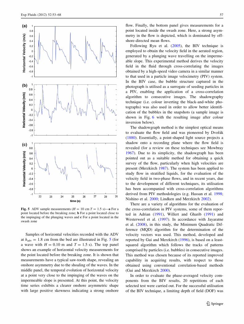
Samples of horizontal velocities recorded with the ADV

at hadv = 1.8 cm from the bed are illustrated in Fig. 5 (for

a wave with H = 0.10 m and T = 1.5 s). The top panel

shows an example of horizontal velocity measurements for

the point located before the breaking zone. It is shown that

measurements have a typical saw-tooth shape, revealing an

onshore asymmetry due to the shoaling of the waves. In the

middle panel, the temporal evolution of horizontal velocity

at a point very close to the impinging of the waves on the

impermeable slope is presented. At this point, the velocity

time series exhibits a clearer onshore asymmetric shape

with large positive skewness indicating a strong onshore

flow. Finally, the bottom panel gives measurements for a

point located inside the swash zone. Here, a strong asym-

metry in the flow is depicted, which is dominated by off-

shore-directed mean flows.

Following Ryu et al. (2005), the BIV technique is

employed to obtain the velocity field in the aerated region,

generated by a plunging wave travelling on the imperme-

able slope. This experimental method derives the velocity

field in the fluid through cross-correlating the images

obtained by a high-speed video camera in a similar manner

to that used in a particle image velocimetry (PIV) system.

In the BIV case, the bubble structure captured in the

photograph is utilised as a surrogate of seeding particles in

a PIV, enabling the application of a cross-correlation

algorithm to consecutive images. The shadowgraphy

technique (i.e. colour inverting the black-and-white pho-

tographs) was also used in order to allow better identifi-

cation of the bubbles in the snapshots (a sample image is

shown in Fig. 6 with the resulting image after colour

inversion below).

The shadowgraph method is the simplest optical means

to evaluate the flow field and was pioneered by Dvorak

(1880). Essentially, a point-shaped light source projects a

shadow onto a recording plane where the flow field is

revealed (for a review on these techniques see Mowbray

1967). Due to its simplicity, the shadowgraph has been

pointed out as a suitable method for obtaining a quick

survey of the flow, particularly when high velocities are

present (Merzkirch 1987). The system has been applied to

study flow in stratified liquids, for the evaluation of the

velocity field in two-phase flows, and in recent years, due

to the development of different techniques, its utilisation

has been accompanied with cross-correlation algorithms

derived from PIV methodologies (e.g. Hassan et al. 1998;

Nishino et al. 2000; Lindken and Merzkirch 2002).

There are a variety of algorithms for the evaluation of

the cross-correlation in PIV systems, some of them repor-

ted in Adrian (1991), Willert and Gharib (1991) and

Westerweel et al. (1997). In accordance with Jayaratne

et al. (2008), in this study, the Minimum Quadratic Dif-

ference (MQD) algorithm for the determination of the

velocity vectors was used. This method, developed and

reported by Gui and Merzkirch (1996), is based on a least-

squared algorithm which follows the tracks of patterns

comprised by particles (i.e. bubbles) in consecutive images.

This method was chosen because of its reported improved

capability in acquiring results, with respect to those

obtained using conventional correlation-based methods

(Gui and Merzkirch 2000).

In order to evaluate the phase-averaged velocity com-

ponents from the BIV results, 20 repetitions of each

selected test were carried out. For the successful utilisation

of the BIV technique, a limiting depth of field (DOF) was

-1

-0.8

-0.6

-0.4

-0.2

0

0.2

0.4

0.6

0.8

1H

ori

zon

tal V

elo

city

(m

/s)

(a)

(b)

(c)

Fig. 5 ADV sample measurements (H = 10 cm T = 1.5 s)—a For a

point located before the breaking zone; b For a point located close to

the impinging of the plunging waves and c For a point located in the

swash zone

Exp Fluids (2012) 52:53–68 57

123

defined, representing the focal distance of the camera, at

which objects appear sharp and well focused. The field of

view (FOV) was determined assuming that the lens focuses

on a point at a distance L from the forward nodal point of

the lens (which is sufficiently close to the distance between

the lens front and the point). For the experiments presented

here, the FOV was 70 cm 9 30 cm (1,245 9 505 pixels),

and following Ryu et al. (2005), the DOF was estimated by

means of the formulae proposed by Ray (2002), which can

be expressed as follows: DOF = S - R, where R repre-

sents the nearest limit and S the farthest limit of the DOF.

The estimation of these two edges (S and R) was

undertaken following S = Lf2/(f2 - NLC) and R = Lf2/

(f2 - NLC). In these two expressions, f is the focal length

of the camera focal lens, C represents the value for the

circle of confusion that depends on the property of the

camera (C = 0.01) and N is the f number of the camera

aperture. Bubbles located outside the region defined by the

DOF appear blurred in the captured image, producing an

unclear texture, which has a small effect on the correlation

algorithm used for the determination of the velocity field.

In contrast, bubbles within the DOF appear sharp, with a

clear pattern resulting from the flow. This pattern was

employed in the correlation method for the estimation of

Fig. 6 Top panel: Sample image taken with the high-speed video camera (H = 10 cm T = 1.5 s); bottom panel: Same image using a

shadowgraphy technique for colour inversion

58 Exp Fluids (2012) 52:53–68

123

the resulting velocity vectors. In this study, the error of the

derived velocity associated with the thickness of the DOF

was estimated as 6%. This value is approximately deter-

mined with the values for the photographic parameters

reported in Table 1, by means of the following expression

e = DOF/2L.

Measurements of the same wave test (H = 10 cm;

T = 1.5 s) with different distances from the nodal point of

the lens were taken in order to revise the accuracy of the

instantaneous and phase-averaged velocity measurements

estimated with this technique. The selected L distances are

shown in Table 1, along with the f-stop scale, the pupil

diameter and the focal length of the lens. Mean velocities

for each case were obtained by phase-averaging measured

instantaneous velocities at each phase applying the fol-

lowing equation:

ukh i ¼1

N

XN

l¼1

uðlÞk ¼ Uk ð1Þ

where the symbol hi represents phase-average, uðlÞk is the

k-component velocity obtained from the lth instantaneous

velocity measurement, N is the total number of instanta-

neous velocities at that phase and Uk is the phase-averaged

mean velocity. Therefore, the velocity field is the mean

velocity obtained from ensemble averaging 20 repeated

instantaneous velocity measurements (i.e. N = 20 events).

As a result of the highly turbulent nature of the breaking

process generated by a plunging wave, the instantaneous

images do not match perfectly the mean velocities in some

instants. The initial time for each event was defined as the

instant when the curled free surface of the wave was first

approaching the impermeable slope. All 20 sets of the

instantaneous velocity fields were matched at this moment,

so that errors in the ensemble average due to mismatch of

the cases are minimised.

Figure 7 shows the comparison between the computed

mean velocities (10 events) for the three cases at two

different points on the impermeable slope. For clarity,

Fig. 7a gives the selected positions for the two points

corresponding to the jet of the plunging wave on the

slope (square), and the return flow region in the swash

zone (cross). Figure 7b and c show very good agreement

of the phase-averaged horizontal velocities at both

selected points. In all cases, velocities are obtained using

the same algorithm and same interrogation window size

of 32 9 32 pixels. A median filter is also applied to

eliminate the spurious vectors in the calculated velocity

maps.

Table 2 details the mean velocities and standard devia-

tion estimated for the three test cases. Small differences are

observed in the reported values of ensemble-averaged

quantities, which provide confidence in the reported values

of this study.

2.2 Reynolds-averaged Navier–Stokes model

The numerical model employed in this study, COBRAS,

is a phase- and depth-resolving model which solves the

2DV spatially averaged Reynolds-averaged Navier–

Stokes equations (e.g. Hsu et al. 2002). As this type of

numerical model has been previously described else-

where, only a general description is presented here. For

more details, readers are referred to the papers of Lin

and Liu (1998a, b) and Liu et al. (1999) where the

equations’ derivation, boundary and initial conditions and

the numerical implementation of the model are presented

in detail. The spatially averaged Navier–Stokes equations

are

o uih ioxi¼ 0 ð2Þ

o uih iotþ uj

� � o uih ioxj¼ � 1

qo p0h ioxiþ gi þ

1

q

o sij

� �

oxj� o u00ou00h ii

oxj

ð3Þ

where the instantaneous velocity, u, and pressure, p0, fields are

decomposed into spatially averaged quantities, �h i, and

spatially fluctuating quantities, �h i00, i.e., ui ¼ uih i þ u00i� ��

n

and p0 ¼ �p0 þ p000 where subscripts denote horizontal

(i, j = 1) and vertical (i, j = 2) components, and m is the

molecular viscosity. The second term on the right-hand side

of (3) is the viscous stress tensor of the mean flow, and the

last term of (3) is the correlation of the spatial velocity

fluctuation.

The numerical model was chosen as it details the main

physical processes required to understand the propagation

of plunging breakers over an impermeable slope and, in

particular, the validation of the BIV technique with the

spatio-temporal snapshots of the velocity field derived by

the model. Although this model has been extensively val-

idated in the laboratory on a small scale (Garcia et al. 2004;

Lara et al. 2006) and a large scale (Pedrozo-Acuna et al.

2010), this work is the first to compare numerical results

against spatio-temporal velocity snapshots measured by

means of the BIV technique. The region of interest covers

Table 1 Fastec HighSpec1 camera parameters

L1 L2 L3

f Stop scale f/8.0 f/5.6 f/5.6

Pupil diameter (mm) 3.125 4.464 4.464

Lens focal length (mm) 25 25 25

Distance from the forward nodal point of the lens

L (m) 1.13 1.23 1.33

DOF (m) 0.21 0.22 0.18

Exp Fluids (2012) 52:53–68 59

123

the process of the plunging wave impinging on the bed, in

the transition region between the surf and the swash zones.

The numerical model does not consider the air entrain-

ment during the wave breaking. Thus, perfect agreement

between model predictions and observations should not be

expected. The model–data comparison presented here is

carried out with the objective of ensuring that the numer-

ical model is able to qualitatively capture the wave trans-

formation along the impermeable slope. The numerical

discretisation of the domain, based on a convergence test,

was defined with a regular grid of Dx = 0.005 m and

Dz = 0.005 m.

3 Results

3.1 Validation of the BIV technique

The validation of BIV was carried out at two points on the

impermeable slope, one in the surf zone and the other in the

swash zone. In addition, the measurements obtained using

the experimental methods were compared with numerical

results from the RANS model.

Figure 8 compares the temporal evolution of horizontal

velocity in the surf zone at h = 1.8 cm from the bed, for a

wave condition defined by h = 0.44 m, H = 10 cm and

T = 1.5 s. In this figure, the top panel shows the photo-

graphic evidence of the measurements taken with a normal

video camera, whilst the lower panel presents the com-

parison of the ensemble horizontal velocity values derived

from both ADV and BIV measurements against the RANS

model results. The experimental time series (ADV and

BIV) are illustrated along their relative confidence levels

evaluated by l ± r, where l represents the mean value and

r is the standard deviation of the measurement. It is shown

that the measurement techniques are in agreement with

Fig. 7 a Location of selected

points; BIV-derived

instantaneous horizontal

velocities estimated with

different focal distances

(H = 10 m T = 1.5 s) at the jet

(b) and swash zones (c) filledtriangle—L = 0.9 m; filledcircle—L = 1.1 m; filleddiamond—L = 1.0 m.

Estimated mean velocities solidline L = 0.9 m; broken lineL = 1.1 cm; doted line,

L = 1.0 cm

Table 2 Mean velocities and standard deviation of horizontal

velocity estimated with the BIV technique using the three different

focal distances

(cm/s) L1 L2 L3

Uswashh i -43.14 -43.81 -44.67

Ujeth i 116.29 115.37 115.95

Sd Uswashh i 3.29 3.02 4.80

Sd Ujeth i 3.67 4.60 2.45

60 Exp Fluids (2012) 52:53–68

123

each other. However, some differences are identified and

need to be discussed. At the beginning of the time record,

just after the passage of the wave crest (from 0 to 0.5 s), the

uncertainty associated with the ADV measurements is

shown to be larger than that determined for the BIV

measurements. This is due to the nature of the flow, which

at this stage may entrain an important amount of air.

Subsequently, at the start of the flow reversal (t * 0.65 s),

the error in the ADV measurements is significantly

reduced, indicating a better level of confidence than that

shown in the BIV measurements. It is concluded that this is

a consequence of the reduction of air present in the flow,

which confirms a better performance of an ADV in flows

with little amount of air. Moreover, time series determined

with the numerical model exhibit the same behaviour as

those observed with both experimental methods. The

numerical results are mostly within the error bands esti-

mated for the measurements. In particular, the magnitude

of the peak onshore velocity is relatively the same in both

experimental techniques and the RANS model.

Figure 9 shows these comparisons for a point within the

swash zone, where the flow is characterised by the run-up of

the turbulent bore generated by the wave impingement.

Although good agreement of both techniques is generally

reported for most of the events, it is noted that the error bars

shown in the BIV measurements are smaller than those

depicted for the ADV. This demonstrates the better per-

formance of the BIV technique in this zone, where turbu-

lence and bubbles are certainly present in the flow. Indeed,

the greater presence of air in the uprush phase of the flow

(positive velocities) is represented in the large uncertainty

associated with the ADV measurements. On the other hand,

the RANS model estimates appear to be closer to the

measurements only during the uprush phase of the flow. In

the backwash phase of the swash event, the RANS model

clearly overpredicts the offshore velocity. This is explained

by the nature of the numerical model, which does not

consider the effects of the air entrainment in the dynamics

of the flow. In addition, a well-posed bottom boundary

condition is not possible in the numerical model due to the

partial cell treatment which is used to represent the obstacle

(Zhang and Liu 2008). However, the three sets of results are

characterised by a maximum uprush velocity (u is positive

onshore) at the beginning of the event and then the velocity

gradually decreases as the swash runs up the slope, falling to

zero by the time of flow reversal.

3.2 Spatio-temporal evolution of the flow field

The results obtained for the detailed point measurements at

these locations enable a comparison of spatio-temporal

0.5 1 1.5

-1

-0.5

0

0.5

1

Time (s)

Vel

oci

ty (m

/s)

(a)

(b)

Fig. 8 Comparison of the derived ensemble horizontal velocities and

associated error bars (l ± r) in the surf zone for H = 10 cm

T = 1.5 s. a Photographic evidence of the ADV measurements;

b ADV (solid line); BIV (filled circle) and RANS model (broken line)

0 0.5 1 1.5

-1

-0.8

-0.6

-0.4

-0.2

0

0.2

0.4

0.6

0.8

1

time (s)V

elo

city

(m

/s)

(a)

(b)

Fig. 9 Comparison of the derived ensemble horizontal velocities and

associated error bars (l ± r) in the swash zone for H = 10 cm

T = 1.5 s. a Photographic evidence of the ADV measurements;

b ADV (solid line); BIV (filled circle) and RANS model (broken line)

Exp Fluids (2012) 52:53–68 61

123

snapshots obtained using the BIV technique against those

obtained with the RANS model for the wave condition

H = 010 m and T = 1.5 s. Due to the nature of the

numerical model, results of the velocity field for a given

wave height are phase-averaged values.

To enable the BIV comparison, 20 recordings of the

selected wave conditions were used to estimate ensemble

averages for the BIV velocity fields. These were deter-

mined by averaging 20 events for each selected snapshot.

This procedure permits the comparison of the mean vector

velocity plots estimated with the model against those

derived from the BIV measurements.

In Fig. 10, the mean velocity vectors are plotted during

the uprush phase of the flow, obtained from the BIV

technique (top) and those calculated with the RANS model

(lower panel). Results of mean flows derived from the BIV

technique reveal with great detail the complexity of the

flow during the wave impingement over the impermeable

slope, illustrating the resulting splash of water from the

wave impact. Interestingly, the BIV measurements reveal a

vortical structure at the back of the impact point (x =

55 cm; see top, middle and right panels). These measure-

ments show that the maximum velocities of the uprush

phase are associated with the splash of water, which is

characterised by the mixture of water and air incorporated

during the breaking process.

Numerical results for the mean flows during the uprush

phase reveal a qualitatively similar picture of the flow.

However, some differences are clearly identified when

numerical results are compared against BIV measurements,

especially for those instants illustrated in the bottom mid-

dle and right panels. Although the splash of water is

reproduced by the numerical model, the turbulent structure

of the flow is not well captured. This is attributed to the

limitation of the turbulence model and especially the

absence of representation of biphasic flows. This result

points towards the importance of the air in the description

of fluid dynamics within this hydrodynamic region.

On the other hand, Fig. 11 illustrates the mean flows

during the backwash phase of the flow. BIV measurements

illustrate a clear predominance of offshore flows with a

more uniform flow structure during this phase in compar-

ison with that depicted during the uprush. The flow

homogeneity during the backwash is the result of the dis-

sipation of turbulence and the destruction of the bubbles

within the fluid, which restore the single-phase nature of

the flow (water only). These characteristics are also

reflected in the representation of the measured mean

backwash flows by the numerical description as shown in

the lower panels. Here, the structure of the velocity field

estimated with the numerical model shows better agree-

ment with the BIV measurements. However, the magnitude

of the offshore flow is clearly overestimated. As mentioned

earlier, these differences are due to the role of air in the

flow dynamics.

In order to determine the dominance of the flow towards

the onshore or offshore direction, the velocity field is

decomposed in mean horizontal and vertical components to

provide a more detailed comparison between BIV mea-

surements and results from the RANS model. Figure 12

shows the comparison of mean horizontal velocities during

the uprush phase of a plunging wave travelling on the slope

(H = 10 cm and T = 1.5 s). The spatio-temporal maps of

the mean horizontal flow field depict instants immediately

before (a), during (b) and after (c) wave impact. The top

panels illustrate the mean horizontal flow field determined

with the BIV method, whilst the numerical model results

are shown below. Interestingly, in all the panels, qualita-

tively good agreement is found during the uprush phase of

the flow. Experimental and numerical results show close

agreement at the wave crest (left panels—time: 67.8 s). In

contrast, the swash lens, running down the slope, shows

Fig. 10 Comparison of phase-averaged horizontal velocity during the uprush of a plunging wave (H = 10 m T = 1.5 s). Top panels—BIV

measurements and bottom panels—RANS model results

62 Exp Fluids (2012) 52:53–68

123

small differences in the magnitude of offshore velocities,

with greater values for the numerical results.

In the centre sections of the figure, results for the

moment at which the overturning jet impinges on the slope

are shown (time = 67.84 s). At these moments, the overall

behaviour of the flow is well described by the numerical

model. Large positive onshore velocities are due to the

wave-impact process, whilst an offshore velocity is seen

close to the impact point. It is evident that the observed

flow separation in the swash tongue is a result of the wave

impact on the backwash phase of the flow.

The right-hand panels present the results an instant after

the wave impact. Here, the differences between the

experimental and numerical flow fields are even more

evident. The resulting splash from the impact process is

clearly larger in the BIV results than those of the numerical

model. Again, this might be accounted for by the single-

phase nature of the numerical description of the flow.

However, despite these differences, the overall magnitudes

of horizontal velocities shown in both panels are in close

agreement. This indicates that, within its limitations, the

numerical description is doing a fair job in the reproduction

of the experiments.

Figure 13 gives the vertical velocities for the same

moments as those shown in Fig. 12. During the initial stage

of the uprush of the plunging wave, a reduced contribution

of the vertical velocities is given by the BIV method, with

positive vertical velocities in the face of the wave under the

crest. This phenomenon is reproduced by the numerical

model, with slightly higher vertical velocities. Here, the

limitations of the BIV method are evident as a significant

portion of the field of view appears white. This does not

mean that vertical velocities are null but reflects the

absence of bubbles in the fluid. Indeed, small vertical

velocities are reported in numerical results for the swash

lens (lower panel). A better picture is seen in the middle

panels, which show the instant the plunging wave impinges

on the slope. Similar patterns of behaviour are observed in

the results of the numerical model; in particular, a strong

vertical jet surrounded by two regions of positive vertical

velocities is seen. However, once again a slight overpre-

diction in the magnitude of vertical velocities is identified.

Fig. 11 Comparison of phase-averaged vertical velocity during the backwash of a plunging wave (H = 10 m T = 1.5 s). Top panels—BIV

measurements and bottom panels—RANS model results

Fig. 12 Comparison of phase-averaged horizontal velocity during the uprush of a plunging wave (H = 10 m T = 1.5 s). Top panels—BIV

measurements and bottom panels—RANS model results

Exp Fluids (2012) 52:53–68 63

123

This is attributed to the need of some representation of the

effect of air entrainment in the velocity field, which is

indeed present in the experimental data. This limitation is

even more evident in the right-hand panels here, where a

later stage of the jet is shown. BIV results show a con-

siderable spread in the plume of water resulting from the

impact process, whilst the numerical model results for the

splash are smaller, with higher velocities. The reported

differences in velocities between the numerical model and

the BIV technique at this instant may be regarded as the

effect of air compressibility in the dynamics of the jet of

water.

The nature of the velocity field in the second phase of

the swash event is seen in Fig. 14, which gives the results

for instants of horizontal velocity in the backwash phase.

As in the previous figures, the top panels illustrate snap-

shots derived from the BIV technique and the bottom

shows the numerical results obtained from the RANS

model. It can be seen that in all the events, the agreement

found is better than in the uprush phase. The swash lens is

shown to have a predominant offshore-directed flow

(negative velocities) in all the instants illustrated. The left-

hand panels present the start of the backwash phase, which

is identified with a thicker swash lens. The horizontal

velocity derived by the BIV technique shows negative

values with patches of white areas, which indicate the

reduction in the number of bubbles present in the fluid at

this stage. The middle panels show a thinning in the swash

lens and a more uniform flow in this phase of the event.

Both the BIV technique and the RANS model identify

small variations along the water column in the values of

horizontal velocities. However, the overestimation of the

magnitude of the horizontal velocity observed in the

numerical results is again identified. A more intense off-

shore flow is present in the bottom panel. It is considered

that this is the consequence of the single-phase nature (only

water) of the numerical description and/or limitations in the

present numerical set-up to resolve the wave boundary

layer dynamics in this region. Despite these identified

limitations, it is fair to say that despite the differences, the

numerical model does a good job of predicting flow

velocities in the region. The right-hand panels illustrate the

Fig. 13 Comparison of phase-averaged vertical velocity during the uprush of a plunging wave (H = 10 m T = 1.5 s). Top panels—BIV

measurements and bottom panels—RANS model results

Fig. 14 Comparison of phase-averaged horizontal velocity during the backwash phase of a plunging wave (H = 10 m T = 1.5 s). Top panels—

BIV measurements and bottom panels—RANS model results

64 Exp Fluids (2012) 52:53–68

123

end of the backwash phase. At this stage, the swash lens is

thinner in both measurements and computed values of

horizontal velocities, although the numerical results are

slightly larger than those obtained using the BIV technique.

This confirms the results presented in the comparison of the

horizontal velocity time series shown in Fig. 9, where both

ADV measurements and BIV offshore flows are of similar

magnitudes. This may indicate that in order to describe the

backwash velocities more accurately, it is necessary to

include the water/air interactions in this region. Indeed,

overestimation of offshore swash velocities has also been

reported with field measurements and the use of a depth-

averaged model based on the non-linear shallow water

equations (NLSWE) (Raubenheimer 2002).

Figure 15 presents the vertical velocities associated with

the same instants as those in Fig. 14. In all panels, it is

shown that the vertical component of the velocity is small.

This indicates the predominance of the horizontal compo-

nent in the behaviour of the fluid in this region and

therefore a hydrostatic pressure field prevails. Vertical

velocities generated with the numerical model are also

consistent with this behaviour.

The process of a plunging wave breaking on an imper-

meable slope triggers violent turbulent motions of fluid

particles; this is clear in both the BIV- or RANS-derived

velocity fields shown in Figs. 10 and 11. The air bubbles

generated during wave breaking make these vortices visi-

ble, as is clearly illustrated in the colour-inverted images of

the BIV results (top panels Figs. 10 and 11).

The horizontal and vertical motions are highly coherent

and thus most of their contributions come from the mean

flow motions which are two dimensional in the laboratory

experiment. On a real beach, the detailed mechanisms of

vorticity generation are highly complex, as the process is

tridimensional (i.e. vortex stretching) and the potential flow

hypothesis is no longer valid. However, in order to enable a

comparison of the mean vorticity dynamics for both uprush

and backwash phases, we derive the mean vorticity asso-

ciated with the mean velocity field at the same instants as

shown in Figs. 10 and 11. This exercise is carried out to

qualitatively determine whether the model reproduces the

measured vorticity resulting from the propagation of the

plunging wave over the slope. It should be noted that

the coarse spatial resolution of the BIV velocity measure-

ments only provides a relative, rather than absolute, value

of the vorticity (Ryu and Chang 2008). On the other hand,

Lin and Liu (1998b) pointed out that the numerical model

assumes the validity of the eddy viscosity hypothesis,

which means that the vortex stretching mechanism will not

be significant in the derived mean flows, and the mean

vorticity will be redistributed only by advection and

diffusion.

The vorticity at a given point is calculated using circu-

lation from the velocities of its eight neighbouring points

as:

Xi;j ¼Ci;j

4DxDzð4Þ

where X is vorticity, C ¼H

v~ � dl~ is circulation and Dx and

Dz are the distances between the adjacent points in the

x and z directions.

Figure 16 presents the mean vorticity field for the

uprush phase of the swash when the plunging wave is

impinging on the slope. The cold colours (blue) represent

negative vorticity, whilst the warm colours (red) represent

positive vorticity (counter clockwise). Both BIV and

numerical results show that the majority of the vorticity is

generated around the overturning of the wave front. Indeed,

for the three instants presented, the vorticity has the same

rotational direction as the overturning jet. Figure 16(mid-

dle) shows the moment of the wave impact on the slope.

Here, there is a small region close to the impact point

Fig. 15 Comparison of phase-averaged vertical velocity during the backwash phase of a plunging wave (H = 10 m T = 1.5 s). Top panels—

BIV measurements and bottom panels—RANS model results

Exp Fluids (2012) 52:53–68 65

123

where positive and negative vorticity coexist. The highest

values of mean vorticity are related to the wave impact

resulting from the plunging jet of water touching on the

backwash tongue.

The mean vorticity calculated for the backwash phase of

the flow is shown in Fig. 17, where a considerable reduc-

tion in the vorticity is illustrated in all panels. In general,

good agreement is found in the comparison of the vorticity

structure along the slope. However, during this phase, it is

evident that vorticity results derived from the BIV mean

velocity field do not illustrate in detail the vorticity diffu-

sion which is observed in results from the RANS model.

Despite the differences, the order of magnitude of the

measured and modelled mean vorticity O(10 s-1) is

similar to that reported in other experimental studies

(Nadaoka et al. 1989; Petti et al. 1994). These qualitative

comparisons provide some confidence in the results pre-

sented here.

4 Conclusions

The work presented here describes the validation of a non-

intrusive method to measure velocity fields induced by

plunging waves from the impinge point and into the swash

zone in the laboratory. Measurements of the velocity field

obtained by the bubble image velocimetry (BIV) technique

were compared to single-point measurements (ADV) along

with their relative confidence levels. Results in the surf zone

show that ADV measurements contain less uncertainty than

those derived from the BIV due to the slight presence of

bubbles in the flow, indicating a better performance of this

instrument in this region. This is ascribed to the nature of

the flow in a region where strong turbulence and aeration

are not yet fully developed. Notably, time series determined

with the numerical model illustrated a similar trend to those

recorded with both experimental methods (i.e. numerical

results are within the estimated error bands).

Fig. 16 Comparison of mean vorticity during the uprush phase of a plunging wave (H = 10 m T = 1.5 s). Top panels—BIV measurements and

bottom panels—RANS model results

Fig. 17 Comparison of mean vorticity during the backwash phase of a plunging wave (H = 10 m T = 1.5 s). Top panels—BIV measurements

and bottom panels—RANS model results

66 Exp Fluids (2012) 52:53–68

123

On the other hand, in the swash zone, although agree-

ment between both techniques is reported for most of the

duration of the event, a different picture is revealed. The

error bars shown for the BIV measurements are smaller

than those depicted for the ADV, illustrating a better per-

formance of the BIV technique in a region where bubbles

are obviously present in the flow. It is reflected that the

greater presence of air in the flow is due to the propagation

of a turbulent bore generated by the wave impingement.

A high-resolution numerical model based on the Rey-

nolds-averaged Navier–Stokes (RANS) equations was used

to evaluate the transient two-dimensional description of the

flow field under plunging breakers. Good agreement was

noted for numerically derived surf zone velocities, whilst in

the swash zone, an overprediction of the offshore flow was

identified. This is thought to be a consequence of the single-

phase nature (only water) of the numerical description.

However, despite this identified limitation, the numerical

model does a fair job of predicting flow velocities within both

regions. Snapshots of the spatio-temporal nature of the flow

field derived by this experimental method (BIV) were also

compared to those computed with the RANS model. Good

agreement was also found in the overall behaviour of the flow

throughout the entire swash event. However, when consid-

ering plunging breakers, the numerical model tends to

overpredict the velocity field as compared with that derived

by the BIV technique. Differences between BIV velocity

estimations and numerical model predictions can be ascribed

to the effects of air compressibility in the dynamics of the

resulting jet of water (after the wave impact), which indicates

the importance of considering the dynamics of the air/water

mixture when an accurate modelling of this type of breaker is

sought. Both BIV and numerical results show that the

majority of the vorticity is generated around the overturning

of the wave front with highest values of mean vorticity

related to the wave impact resulting from the plunging jet of

water touching on the backwash tongue.

An advantage of the BIV technique is that surf–swash zone

velocities can be obtained at any point in the cross-shore

direction, even if the flow is highly aerated. Moreover, the

technique is non-intrusive. In contrast, disadvantages of the

method are that the derivation of a velocity field depends on

the presence of bubbles in the fluid, and no information is

derived if bubbles are not present in the flow. Therefore, under

hydrodynamic conditions induced by plunging waves, the

BIV technique was shown to be a good complementary tool to

numerical models in the estimation of velocity fields in the

laboratory, where the fluid is highly aerated and the use of

other methods is not possible.

Acknowledgments The research was supported in part by research

grants from the National Autonomous University of Mexico (PAPIIT

IN106610) and the research fund provided by the Engineering

Institute (A2). We would like to thank the following for their assis-

tance with the laboratory work described in this paper: Ariadna Cruz

Quiroz, Jorge G. Gonzalez Armenta, Miguel A. Laverde Barajas and

Juan P. Rodrıguez Rincon.

References

Adrian RJ (1991) Particle-imaging techniques for experimental fluid

mechanics. Annu Rev Fluid Mech 23:261–304

Bakhtyar AMR, Barry DA, Yeganeh-Bakhtiary A, Zou QP (2010)

Air-water two-phase flow modeling of turbulent surf and swash

zone wave motions. Adv Water Resour 33(12):1560–1574

Brocchini M, Baldock TE (2008) Recent advances in modelling

swash zone dynamics: Influence of Surf-Swash interaction on

nearshore hydrodynamics and morphodynamics. Rev Geophys

46:RG3003. doi:10.1029/2006RG000215

Cowen EA, Sou IM, Liu PLF, Raubenheimer B (2003) Particle image

velocimetry measurements within a laboratory-generated swash

zone. J Eng Mech 129(10):1119–1129

Cox DT, Kobayashi N (2000) Identification of intense, intermittent

coherent motions under shoaling and breaking waves. J Geophys

Res 105:14223–14236

Cox DT, Shin S (2003) Laboratory measurements of void fraction and

turbulence in the bore region of surf zone waves. J Eng Mech

Res 129:1197–1205

Cox DT, Kobayashi N, Okayasu A (1996) Bottom shear stress in the

surf zone. J Geophys Res 101:14337–14348

Dvorak V (1880) Uber eine neue einfache Art der Schlierenbeobach-

tung. Ann der Physik 245(3):502–512. doi:10.1002/andp.1880

2450309

Garcia N, Lara JL, Losada IJ (2004) 2-D numerical analysis of near-

field flow at low-crested permeable breakwaters. Coastal Eng

51(10):991–1020

Govender K, Mocke GP, Alport MJ (2002a) Video-imaged surf zone

wave and roller structures and flow fields. J Geophys Res

107(C7):3072

Govender K, Alport MJ, Mocke G, Michallet H (2002b) Video

measurements of fluid velocities and water levels in breaking

waves. Physica Scripta T97:152–159

Govender K, Mocke GP, Alport MJ (2004) Dissipation of isotropic

turbulence and length-scale measurements through the wave roller

in laboratory spilling waves. J Geophys Res 109(C8):C08018

Gui L, Merzkirch W (1996) A method of tracking ensembles of

particle images. Exp Fluids 21:465–468

Gui L, Merzkirch W (2000) A comparative study of the MQD method

and several correlation-based PIV evaluation algorithms. Exp

Fluids 28:36–44

Hassan YA, Schmidl WD, Ortiz-Villafuerte J (1998) Investigation of

three-dimensional two-phase flow structure in a bubbly pipe

Meas. Sci Technol 9:309–326

Holland KT, Puleo JA, Kooney TN (2001) Quantification of swash

flows using video-based particle image velocimetry. Coastal Eng

44(2):65–77

Hsu T-J, Sakakiyama T, Liu PL-F (2002) A numerical model for

wave motions and turbulence flows in front of a composite

breakwater. Coastal Eng 46(1):25–50

Huang ZC, Hsiao SC, Hwung HH, Chang KA (2009) Turbulence and

energy dissipations of surf-zone spilling breakers. Coastal Eng

56(7):733–746

Huang ZC, Hwung HH, Hsiao SC, Chang KA (2010) Laboratory

observation of boundary layer flow under spilling breakers in

surf zone using particle image velocimetry. Coastal Eng 57(3):

343–357

Exp Fluids (2012) 52:53–68 67

123

Jayaratne R, Hunt-Raby A, Bullock G, Bredmose H (2008) Individual

violent overtopping events: new insights. In: Proceedings of the

31th international conference on coastal engineering, Hamburg,

World Scientific, 1-13 pp

Kimmoun O, Branger H (2007) A particle image velocimetry

investigation on laboratory surf-zone breaking waves over a

sloping beach. J Fluid Mech 588:353–397

Kimmoun O, Branger H, Zucchini B (2004) Laboratory PIV

measurements of wave breaking on a beach. In: Proceedings of

the 14th international offshore and polar engineering conference,

May 23–28

Lara JL, Garcia N, Losada IJ (2006) RANS modelling applied to

random wave interaction with submerged permeable structures.

Coastal Eng 53(3–4):395–417

Lin P, Liu PL-F (1998a) A numerical study of breaking waves. J Fluid

Mech 359:239–264

Lin P, Liu PL-F (1998b) Turbulence transport, vorticity dynamics,

and solute mixing under plunging waves in surf zones. J Geophys

Res 103(15):15677–15694

Lindken R, Merzkirch W (2002) A novel PIV technique for

measurements in multi-phase flows and its application to two-

phase bubbly flows. Exp Fluids 33:814–825

Liu PL-F, Lin P, Chang KA, Sakakiyama T (1999) Numerical

modeling of wave interaction with porous structures. J Waterway

Port Coastal Ocean Eng 125:322–330

Masselink G, Puleo JA (2006) Swash-zone morphodynamics. Cont

Shelf Res 26(5):661–680

Masselink G, Evans D, Hughes MG, Russell P (2005) Suspended

sediment transport in the swash zone of a dissipative beach.

Marine Geol 216(3):169–189

Merzkirch W (1987) Flow visualization, 2nd edn. Academic Press,

New York

Mowbray DE (1967) The use of schlieren and shadowgraph

techniques in the study of flow patterns in density stratified

liquids. J Fluid Mech 27(3):595–608. doi:10.1017/S00221120

67000564

Nadaoka K, Hino M, Koyano Y (1989) Structure of the turbulent flow

field under breaking waves in the surf zone. J Fluid Mech

204:359–387

Nishino K, Kato H, Torii K (2000) Stereo imaging for simultaneous

measurement of size and velocity of particles in dispersed two-

phase flow Meas. Sci Technol 11:633–645

O’Donoghue T, Pokrajac D, Hondebrink LJ (2010) Laboratory and

numerical study of dambreak-generated swash on impermeable

slopes. Coast Eng 57(5):513–530. doi:10.1016/j.coastaleng.

2009.12.007

Pedrozo-Acuna A, Simmonds DJ, Reeve DE (2008) Wave-impact

characteristics of plunging breakers acting on gravel beaches.

Mar Geol 253(1):26–35. doi:10.1016/j.margeo.2008.04.013

Pedrozo-Acuna A, Torres-Freyermuth A, Zou QP, Hsu T-J, Reeve DE

(2010) Diagnostic investigation of impulsive pressures induced

by plunging breakers impinging on gravel beaches. Coastal Eng

57(3):252–266. doi:10.1016/j.coastaleng.2009.09.010

Pedrozo-Acuna A, Ruiz de Alegrıa-Arzaburu A, Torres-Freyermuth

A, Mendoza E, Silva R (2011) Laboratory investigation on

pressure gradients induced by plunging breakers. Coastal Eng

58(8):722–738. doi:10.1016/j.coastaleng.2011.03.013

Petti M, Longo S (2001) Turbulence experiments in the swash zone.

Coastal Eng 43:1–24

Petti M, Quinn PA, Liberatore C, Easton WJ (1994) Wave velocity

field measurements over a submerged breakwater. In: Proceed-

ings of the 24th international conference on coastal engineering,

pp 525–539

Raubenheimer B (2002) Observations and predictions of fluid

velocities in the surf and swash zones. J Geophys Res 107(C11):

3190. doi:10.1029/2001JC001264

Ray SD (2002) Applied photographic optics. Focal, Oxford,

pp 215–233

Ryu Y, Chang K-A (2008) Green water void fraction due to breaking

wave impinging and overtopping. Exp Fluids 45:883–898

Ryu Y, Chang K-A, Lim H-J (2005) Use of bubble image velocimetry

for measurement of plunging wave impinging on structure and

associated greenwater. Meas Sci Technol 16:1945–1953

Ryu Y, Chang K-A, Mercier R (2007) Runup and green water

velocities due to breaking wave impinging and overtopping. Exp

Fluids 43:555–567

Ting FCK (2006) Large-scale turbulence under a solitary wave. Coast

Eng 53(5–6):441–462

Ting FCK, Kirby JT (1994) Observation of undertow and turbulence

in a laboratory surf zone. Coast Eng 24(1–2):51–80

Ting FCK, Kirby JT (1995) Dynamics of surf-zone turbulence in a

strong plunging breaker. Coast Eng 24:177–204

Ting FCK, Kirby JT (1996) Dynamics of surf-zone turbulence in a

spilling breaker. Coast Eng 27:131–160

Westerweel J, Dabiri D, Gharib M (1997) The effect of a discrete

window offset on the accuracy of cross-correlation analysis of

digital PIV recordings. Exp Fluids 23:20–28

Willert CE, Gharib M (1991) Digital particle image velocimetry. Exp

Fluids 10:181–193

Zhang Q, Liu PL-F (2008) A numerical study of swash flow generated

by bores. Coastal Eng 55(12):1113–1134

68 Exp Fluids (2012) 52:53–68

123