Swash zone boundary conditions derived from opticalremote sensing of swash zone flow patterns

H. E. Power,1 R. A. Holman,2 and T. E. Baldock1

Received 13 October 2010; revised 27 January 2011; accepted 3 February 2011; published 15 June 2011.

[1] Optical remote sensing is used to measure flow patterns in the swash zone. Timestackimages are analyzed to measure the asymmetry and the relative duration of the inflow intothe swash zone. This varies significantly between individual swashes, contrary to theclassical analytical swash model for runup induced by bores, which predicts a similar flowpattern for all events. For swash forced by breaking bores, the gradient of the x‐t locusof flow reversal varies over a wide range and flow reversal can occur simultaneouslyacross the whole swash zone. This variation of the gradient of the locus of flow reversal inx‐t space can be parameterized in terms of a single free variable in recent solutions to thenonlinear shallow water equations, which fully defines the swash boundary inflowcondition. Consistent with the theory, the horizontal runup, the swash period, and theswash similarity parameter were observed to be independent of the swash inflowconditions but the flow asymmetry is not. Only a weak correlation was observed betweenthe swash boundary condition and the Iribarren number and beach slope. Conversely, theanalysis suggests that the degree of swash‐swash interaction does influence the swashboundary condition and the resulting internal flow kinematics. The variation in inflowconditions is expected to influence the magnitudes of the velocity moments within theswash zone and therefore sediment transport rates.

Citation: Power, H. E., R. A. Holman, and T. E. Baldock (2011), Swash zone boundary conditions derived from optical remotesensing of swash zone flow patterns, J. Geophys. Res., 116, C06007, doi:10.1029/2010JC006724.

1. Introduction

[2] Swash zone dynamics are a fundamental componentof the forcing for the beach system. The swash zone linksthe terrestrial and marine environments and is an importantmechanism of sediment exchange between the surf zone andsubaerial beach [Masselink and Puleo, 2006]. However,sediment transport is generally poorly predicted, particularlyaccretionary conditions [Elfrink and Baldock, 2002;Masselinkand Puleo, 2006]. To address this, a recent focus of study hasbeen the advection of sediment into the swash zone, whichbalances the natural asymmetry of the swash hydrodynamicsthat favor the export sediment from the swash zone [Hugheset al., 1997; Puleo et al., 2000; Pritchard and Hogg, 2005;Masselink and Puleo, 2006]. Both the quantity of advectedsediment and the flow asymmetry depend on the flow char-acteristics, particularly the duration of the inflow and the timeat which the flow reverses between uprush and backwash. Inviolation of the classical Shen and Meyer [1963] model,observations show considerable scatter or variability of theseparameters on a swash‐by‐swash basis [Raubenheimer, 2002;Puleo et al., 2003; Hughes and Baldock, 2004; Houser and

Barrett, 2010]. Shen and Meyer [1963] found that the swashis independent of the variability of the bore conditions in theinner surf zone, i.e., the solution depends on a fixed seawardboundary condition and initial shoreline velocity. However,Guard and Baldock [2007] showed that different boundaryconditions provide alternative solutions of the nonlinearshallow water wave equations. These different boundaryconditions describe different forcing or inflow conditions atthe seaward swash boundary, and allow the solutions todescribe variability in the internal flow field for different swashevents. In nondimensional form, the solutions are controlledby a single free boundary condition parameter, k, whichcontrols the mass and momentum flux into the swash zone. Indimensional form, or physical parameters, the characteristicsof the flow are controlled by the wave or bore height, waveor bore period, waveshape and asymmetry, and incidentvelocity [Elfrink and Baldock, 2002]. In addition, the innersurf conditions experienced by the incident bore depend onswash‐swash interactions, wave‐induced currents and longwaves, all of which have the potential to influence themomentum flux into the swash zone.[3] The Shen andMeyer [1963] model is a special solution to

the nonlinear shallow water (NLSW) equations [Peregrine andWilliams, 2001; Pritchard and Hogg, 2005], and representsan asymptotic description of the flow close to the wave tip fora single and specific boundary condition. It has been shown toclosely approximate the shoreline motion in the swash zone,particularly if frictional effects at the wave tip are included

1School of Civil Engineering, University of Queensland, St Lucia,Queensland, Australia.

2College of Oceanic and Atmospheric Sciences, Oregon StateUniversity, Corvallis, Oregon, USA.

Copyright 2011 by the American Geophysical Union.0148‐0227/11/2010JC006724

JOURNAL OF GEOPHYSICAL RESEARCH, VOL. 116, C06007, doi:10.1029/2010JC006724, 2011

C06007 1 of 13

[Hughes, 1995; Baldock and Holmes, 1999; Puleo andHolland, 2001]. However, it does not accurately describethe internal hydrodynamics, i.e., the flow depth and velocity[Baldock et al., 2005; Guard and Baldock, 2007]. Further, theapparent scatter in the asymmetry between uprush andbackwash flow durations, as widely observed in the field andlaboratory [Kemp, 1975; Raubenheimer et al., 1995; Baldockand Holmes, 1997; Masselink and Hughes, 1998;Raubenheimer, 2002], is not consistent with the Shen‐Meyersolution. On fine‐grained sandy beaches, these differences arenot likely to be a result of friction or infiltration, which pri-marily influence the flow close to the leading edge, i.e., theshoreline motion. For example, Packwood [1983] showsnegligible influence from infiltration during runup on fineand medium sand beaches. In addition, the classical solu-tion is hydrodynamically similar for all swash events andsimply scales on the runup amplitude [Peregrine andWilliams, 2001]; i.e., after the initial bore collapse, theinternal properties of the swash are independent of the con-ditions at the seaward swash boundary irrespective of the surfzone conditions. This is inconsistent with a wide range ofobservations of variability in the hydrodynamics, sedimenttransport and morphological change, where the latter alsovaries on a swash‐by‐swash basis [Waddell, 1976; Baldock,2009; Turner et al., 2009].[4] The Shen‐Meyer solution neglects the mass and

momentum of the flow behind the incident bore front, andhence any variability in these physical parameters as a resultof variability in the inner surf conditions. Recognizing this,Guard and Baldock [2007] developed new numerical solu-tions to the nonlinear shallow water equations that allowvariable swash boundary conditions. The variable swashboundary conditions do not affect the shoreline motion,which does not differ from that predicted by Shen and Meyer[1963]; only the internal kinematics, in particular the flowasymmetry and time of flow reversal, are different. Thephysical cause for the different flow behavior is the inclusionof the mass and momentum of the flow behind the incidentbore front, i.e., a more sustained inflow across the seawardboundary of the swash zone.[5] The importance of the swash zone boundary condition

was illustrated by Baldock et al. [2005], who showed thatreal swash overtopping volumes were much greater thanpredicted by the Shen‐Meyer model [cf. Peregrine andWilliams, 2001] and by Pritchard [2009] who demonstratedthat sediment transport predictions differ between the Shen‐Meyer model [cf. Pritchard and Hogg, 2005] and the morerecent solutions. Differences in asymmetry in the flow fieldbetween different swash events are likely to lead to differ-ences in net sediment transport directions [Elfrink andBaldock, 2002; Pritchard, 2009]. Indeed, Houser andBarrett [2010] show differences between periods of accre-tion or erosion of the beach face could be separated by thedifferent relative time of flow reversal in the swash zone.However, while the field data of Masselink and Hughes[1998], Raubenheimer [2002], Hughes and Baldock [2004],and Houser and Barrett [2010] suggest that the time of flowreversal is quite variable and different from the behaviorpredicted by the Shen‐Meyer model, this has not been relatedto the different possible solutions of the nonlinear shallowwater equations for natural conditions. Further, the variationof the incoming mass and momentum for different surf and

swash conditions has not been identified and quantified inthe field. Identifying such variations is important for improvedwave by wave and stochastic descriptions of overtoppingof structures and dunes, and for modeling the sediment fluxacross the surf‐swash boundary.[6] This paper addresses this issue and presents the first

comprehensive data set showing the variation in the swashinflow conditions on real beaches and that this variation isconsistent with the recent solutions of the NLSW equations.The data suggest that this is the reason why natural boreinduced swash is different from the Shen‐Meyer model,instead of being a result of other processes which mightmake the swash deviate from the Shen‐Meyer solution (e.g.,the effects of infiltration and friction). We also show thedevelopment of a new application of remote sensing toprovide quantitative data which can be directly compared tonumerical model results. Section 2 outlines the numericalmodel and illustrates the importance of the boundary con-dition for the swash hydrodynamics. Section 3 describes themethods of data collection, the preprocessing required toobtain timestack images and the method used to identify andverify the locus of flow reversal and the boundary conditionparameter, k, for individual swash events. The results of thisanalysis are presented in section 4 together with a statis-tical analysis of the relationship between k and varioustime‐averaged offshore and individual wave characteristics.Section 5 presents a discussion of the data and illustrateshow remote measurements of the locus of flow reversal andk could be used to infer other parameters, particularly mag-nitudes of velocity moments. Final conclusions are outlinedin section 6.

2. Swash Hydrodynamics Model

[7] The Guard and Baldock [2007] model solves a non-dimensional form of the NLSW equations written as

@h

@tþ @ uhð Þ

@x¼ 0

@u

@tþ u

@u

@xþ @h

@xþ 1 ¼ 0;

ð1Þ

where x is the dimensionless cross‐shore distance, t is thedimensionless time, h is the dimensionless water depth mea-sured perpendicular to the slope, and u is the dimensionlessflow velocity [Peregrine and Williams, 2001]. These param-eters are related to the dimensional variables as follows:

x ¼ sin �swð Þx*a

; t ¼ sin �swð Þt*ffiffiffig

a

r; h ¼ cos�swð Þh*

a; u ¼ u*ffiffiffiffiffi

gap ;

ð2Þ

where * denotes dimensional variables, bsw is angle of thebeach face in the swash zone, g is the acceleration due togravity, and 2a is the vertical excursion of the undisturbedswash. Substituting for the nondimensional shallow waterwave speed, c =

ffiffiffih

p, (1) may be rearranged to obtain

@

@tþ uþ cð Þ @

@x

� �uþ 2cþ tð Þ ¼ 0

@

@tþ u� cð Þ @

@x

� �u� 2cþ tð Þ ¼ 0:

ð3Þ

POWER ET AL.: SWASH ZONE BOUNDARY CONDITIONS C06007C06007

2 of 13

Introducing the characteristic variables a(x, t) and b(x, t)gives

d

dt� ¼ 0 on

dx

dt¼ uþ c; ð4Þ

d

dt� ¼ 0 on

dx

dt¼ u� c; ð5Þ

where

� x; tð Þ ¼ uþ 2cþ t

� x; tð Þ ¼ u� 2cþ t:ð6Þ

The solutions and model results are controlled by the valueof a(t) on the seaward swash boundary. The Shen‐Meyersolution corresponds to a constant value of a = 2, whichresults in a very thin swash. Guard and Baldock [2007]allowed the value of the characteristic variable on the sea-ward boundary, a, to vary over time, such that

� tð Þ ¼ 2þ kt; ð7Þ

where k is a constant for each individual swash and k = 0corresponds to the Shen‐Meyer solution. Choosing k ≠ 0allows a(t) to vary through time, which is the fundamentaldifference introduced by Guard and Baldock [2007]. Ananalytical form of these solutions was later developed byPritchard et al. [2008], verifying the previous numericalscheme. Initially k was expected to lie in the range 0 < k < 1,where k = 1 corresponds to conditions representative of uni-form incident bores. Hence, the Shen‐Meyer solution isidentical for all swash events, but the Guard‐Baldock modelallows different hydrodynamics for different individual swashevents by specification of different values for the boundarycondition parameter k. Baldock and Hughes [2006] presentedphotographs of incident bores where the water surface ele-vation behind the bore front is horizontal, consistent with nearuniform bore conditions. The solutions in nondimensionalform are independent of beach slope, swash period and runupamplitude. It is therefore important to note that values of kderived from observations should therefore not be dependenton swash beach slope, swash period or runup amplitude,although beach slope does influence the inner surf zoneconditions.[8] Varying the boundary conditions on the seaward

boundary, corresponding to varying a(t) on the incomingcharacteristics, results in deeper and less asymmetric swashflows than those predicted by the Shen‐Meyer solution. Thephysical significance of the characteristic values a and b isshown by writing

u ¼ �þ � � 2t

2c ¼ �� �

4; ð8Þ

which gives the nondimensional volume flux, q, andmomentum flux, M, per unit length of wave crest as

q ¼ uh ¼ 1

32�þ � � 2tð Þ �� �ð Þ2

M ¼ u2h ¼ 1

64�þ � � 2tð Þ2 �� �ð Þ2:

ð9Þ

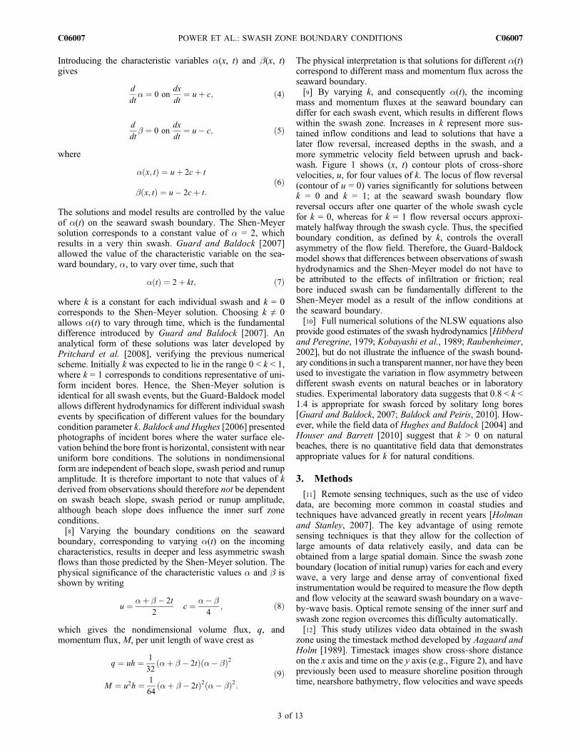
The physical interpretation is that solutions for different a(t)correspond to different mass and momentum flux across theseaward boundary.[9] By varying k, and consequently a(t), the incoming

mass and momentum fluxes at the seaward boundary candiffer for each swash event, which results in different flowswithin the swash zone. Increases in k represent more sus-tained inflow conditions and lead to solutions that have alater flow reversal, increased depths in the swash, and amore symmetric velocity field between uprush and back-wash. Figure 1 shows (x, t) contour plots of cross‐shorevelocities, u, for four values of k. The locus of flow reversal(contour of u = 0) varies significantly for solutions betweenk = 0 and k = 1; at the seaward swash boundary flowreversal occurs after one quarter of the whole swash cyclefor k = 0, whereas for k = 1 flow reversal occurs approxi-mately halfway through the swash cycle. Thus, the specifiedboundary condition, as defined by k, controls the overallasymmetry of the flow field. Therefore, the Guard‐Baldockmodel shows that differences between observations of swashhydrodynamics and the Shen‐Meyer model do not have tobe attributed to the effects of infiltration or friction; realbore induced swash can be fundamentally different to theShen‐Meyer model as a result of the inflow conditions atthe seaward boundary.[10] Full numerical solutions of the NLSW equations also

provide good estimates of the swash hydrodynamics [Hibberdand Peregrine, 1979; Kobayashi et al., 1989; Raubenheimer,2002], but do not illustrate the influence of the swash bound-ary conditions in such a transparent manner, nor have they beenused to investigate the variation in flow asymmetry betweendifferent swash events on natural beaches or in laboratorystudies. Experimental laboratory data suggests that 0.8 < k <1.4 is appropriate for swash forced by solitary long bores[Guard and Baldock, 2007; Baldock and Peiris, 2010]. How-ever, while the field data of Hughes and Baldock [2004] andHouser and Barrett [2010] suggest that k > 0 on naturalbeaches, there is no quantitative field data that demonstratesappropriate values for k for natural conditions.

3. Methods

[11] Remote sensing techniques, such as the use of videodata, are becoming more common in coastal studies andtechniques have advanced greatly in recent years [Holmanand Stanley, 2007]. The key advantage of using remotesensing techniques is that they allow for the collection oflarge amounts of data relatively easily, and data can beobtained from a large spatial domain. Since the swash zoneboundary (location of initial runup) varies for each and everywave, a very large and dense array of conventional fixedinstrumentation would be required to measure the flow depthand flow velocity at the seaward swash boundary on a wave‐by‐wave basis. Optical remote sensing of the inner surf andswash zone region overcomes this difficulty automatically.[12] This study utilizes video data obtained in the swash

zone using the timestack method developed by Aagaard andHolm [1989]. Timestack images show cross‐shore distanceon the x axis and time on the y axis (e.g., Figure 2), and havepreviously been used to measure shoreline position throughtime, nearshore bathymetry, flow velocities and wave speeds

POWER ET AL.: SWASH ZONE BOUNDARY CONDITIONS C06007C06007

3 of 13

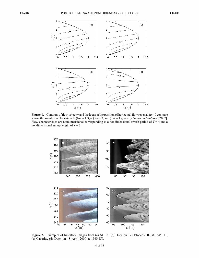
Figure 1. Contours of flow velocity and the locus of the position of horizontal flow reversal (u = 0 contour)across the swash zone for (a) k = 0, (b) k = 1/3, (c) k = 2/3, and (d) k = 1 given byGuard and Baldock [2007].Flow characteristics are nondimensional corresponding to a nondimensional swash period of T = 4 and anondimensional runup length of x = 2.

Figure 2. Examples of timestack images from (a) NCEX, (b) Duck on 17 October 2009 at 1345 UT,(c) Cabarita, (d) Duck on 18 April 2009 at 1540 UT.

POWER ET AL.: SWASH ZONE BOUNDARY CONDITIONS C06007C06007

4 of 13

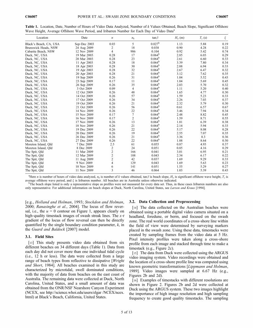
[e.g., Holland and Holman, 1993; Stockdon and Holman,2000; Ranasinghe et al., 2004]. The locus of flow rever-sal, i.e., the u = 0 contour on Figure 1, appears clearly onhigh‐quality timestack images of swash streak lines. The x‐tgradient of the locus of flow reversal can then be directlyquantified by the single boundary condition parameter, k, inthe Guard and Baldock [2007] model.

3.1. Field Sites

[13] This study presents video data obtained from sixdifferent beaches on 34 different days (Table 1). Data fromeach day did not cover more than one individual tidal cycle(i.e., 12 h or less). The data were collected from a largerange of beach types from reflective to dissipative [Wrightand Short, 1984]. All beaches examined in this study arecharacterized by microtidal, swell dominated conditions,with the majority of data from beaches on the east coast ofAustralia. The remaining data were collected at Duck, NorthCarolina, United States, and a small amount of data wasobtained from the ONR/NSF Nearshore Canyon Experiment(NCEX, see http://science.whoi.edu/users/elgar /NCEX/ncex.html) at Black’s Beach, California, United States.

3.2. Data Collection and Preprocessing

[14] The data collected on the Australian beaches wereobtained using a portable digital video camera situated on aheadland, foredune, or berm, and focused on the swashzone. The real world coordinates of a cross‐shore line withinthe field of view were determined by surveying markersplaced in the swash zone. Using these data, timestacks werecreated by sampling frames from the video data at 5 Hz.Pixel intensity profiles were taken along a cross‐shoreprofile from each image and stacked through time to make atimestack (e.g., Figure 2c).[15] The data from Duck were collected using the ARGUS

video imaging system. Video recordings were obtained andthe location of a cross‐shore profile line was computed usingknown geometric transformations [Lippmann and Holman,1989]. Video images were sampled at 6.67 Hz (e.g.,Figures 2b and 2d).[16] Examples of timestacks with different resolutions are

shown in Figure 2. Figures 2b and 2d were collected atDuck using the ARGUS system. These two images highlightthe importance of high image resolution and high samplingfrequency to create good quality timestacks. The sampling

Table 1. Location, Date, Number of Hours of Video Data Analyzed, Number of k Values Obtained, Beach Slope, Significant OffshoreWave Height, Average Offshore Wave Period, and Iribarren Number for Each Day of Video Dataa

Location Date n nk tanb Ho (m) Tz (s) x

Black’s Beach, CA, USA Sep‐Dec 2003 0.03 5 0.027b 1.13 5.88 0.19Brunswick Heads, NSW 24 Aug 2009 2 18 0.038 0.90 4.28 0.22Cabarita Beach, NSW 12 Nov 2009 4 986 0.104 0.92 5.42 0.74Duck, NC, USA 19 Mar 2003 0.28 17 0.064b 2.85 6.03 0.29Duck, NC, USA 20 Mar 2003 0.28 23 0.064b 2.61 6.60 0.33Duck, NC, USA 11 Apr 2003 0.28 18 0.064b 3.39 7.80 0.34Duck, NC, USA 18 Apr 2003 0.28 30 0.064b 2.88 6.94 0.33Duck, NC, USA 19 Apr 2003 0.28 32 0.064b 2.67 6.47 0.32Duck, NC, USA 20 Apr 2003 0.28 21 0.064b 3.12 7.62 0.35Duck, NC, USA 19 Sep 2009 0.26 31 0.064b 1.04 5.52 0.43Duck, NC, USA 23 Sep 2009 0.17 11 0.064b 1.04 5.69 0.45Duck, NC, USA 26 Sep 2009 0.26 35 0.064b 2.03 5.70 0.32Duck, NC, USA 3 Oct 2009 0.09 4 0.064b 1.11 5.20 0.40Duck, NC, USA 12 Oct 2009 0.26 48 0.064b 1.65 4.77 0.30Duck, NC, USA 14 Oct 2009 0.26 57 0.064b 1.59 5.23 0.33Duck, NC, USA 17 Oct 2009 0.26 34 0.064b 2.26 7.03 0.37Duck, NC, USA 19 Oct 2009 0.26 21 0.064b 2.32 5.79 0.30Duck, NC, USA 21 Oct 2009 0.26 56 0.064b 0.61 6.57 0.67Duck, NC, USA 14 Nov 2009 0.26 22 0.064b 3.46 7.94 0.34Duck, NC, USA 15 Nov 2009 0.17 7 0.064b 2.48 8.82 0.45Duck, NC, USA 16 Nov 2009 0.17 2 0.064b 1.59 8.71 0.55Duck, NC, USA 17 Nov 2009 0.26 13 0.064b 1.81 6.39 0.38Duck, NC, USA 18 Nov 2009 0.26 21 0.064b 2.14 5.94 0.33Duck, NC, USA 19 Dec 2009 0.26 22 0.064b 5.17 8.08 0.28Duck, NC, USA 20 Dec 2009 0.26 19 0.064b 2.55 7.07 0.35Duck, NC, USA 26 Dec 2009 0.26 21 0.064b 3.36 8.3 0.36Duck, NC, USA 27 Dec 2009 0.26 22 0.064b 1.88 8.64 0.50Moreton Island, Qld 7 Dec 2009 2.5 61 0.055 0.87 4.93 0.37Moreton Island, Qld 8 Dec 2009 2 24 0.051 0.85 4.16 0.29The Spit, Qld 11 Mar 2009 2 166 0.041 3.01 6.95 0.21The Spit, Qld 12 Mar 2009 2 188 0.043 2.34 6.17 0.22The Spit, Qld 11 Aug 2009 2 42 0.037 1.69 9.29 0.33The Spit, Qld 9 Nov 2009 4 129 0.043 1.69 5.63 0.23The Spit, Qld 10 Nov 2009 6 141 0.051 1.55 5.29 0.27The Spit, Qld 11 Nov 2009 3 46 0.064 1.03 5.39 0.43

aHere n is number of hours of video data analyzed, nk is number of k values obtained, tanb is beach slope, Ho is significant offshore wave height, Tz isaverage offshore wave period, and x is Iribarren number. All beaches are in Australia unless otherwise indicated.

bThe beach slope listed is only a representative slope as profiles were not measured for every data set. Thus, in these cases Iribarren numbers are alsoonly representative. For additional information on beach slopes at Duck, North Carolina, United States, see Larson and Kraus [1994].

POWER ET AL.: SWASH ZONE BOUNDARY CONDITIONS C06007C06007

5 of 13

frequency of these images is 2 and 6.67 Hz respectively.Figure 2a was collected during NCEX (see http://science.whoi.edu/users/elgar/NCEX/ncex.html) and is another exam-ple of a high‐quality timestack; it has a sampling frequencyof 6 Hz. Figure 2c is representative of the data sets collectedin Australia using a portable digital video camera. All datacollected in Australia was sampled at 5 Hz. The time offlow reversal at multiple cross‐shore locations can be easilyidentified in the images, i.e., when the gradients of thestreak lines change sign.

3.3. Calculation of k

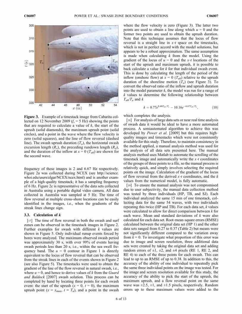
[17] The time of flow reversal in both the swash and surfzones can be observed in the timestack images in Figure 2.Further examples for swash with different k values areshown in Figure 5. Only individual runup events forced bybores were analyzed. The maximum observed swash periodwas approximately 30 s, with over 99% of events havingswash periods less than 20 s, i.e., within the sea swell fre-quency band. The u = 0 contour in Figure 1 is directlyequivalent to the locus of flow reversal that can be observedfrom the streak lines in each of the events shown in Figure 2(see also Figure 5). The timestacks were used to obtain thegradient of the line of the flow reversal in natural swash, i.e.,where u = 0, and hence to derive values of k from the Guardand Baldock [2007] swash solution. This process can becompleted by hand by locating three points for each swashevent: the start of the uprush (x = 0, t = 0), the maximumuprush point (x = xmax, t = Tu), and a point in the swash

where the flow velocity is zero (Figure 3). The latter twopoints are used to obtain a line along which u = 0 and theformer two points are used to obtain the uprush duration.Note that this technique assumes that the locus of flowreversal is a straight line in x‐t space on the timestacks,which is not in perfect accord with the model solutions, butappears to be a robust approximation. The same assumptionis made when calculating k from the model. Using thegradient of the locus of u = 0 and the x‐t locations of thestart of the uprush and maximum uprush, it is possible toback calculate a value for k for that individual swash event.This is done by calculating the length of the period of theinflow (onshore flow) at x = 0 (Tu0) relative to the uprushduration of the shoreline motion (Tu) (see Figure 3). Toconvert the observed ratio of the inflow and uprush durationinto the model parameter k, the model was run for a range ofk values to determine the following relationship betweenTu0/Tu and k

k ¼ 0:77e0:48Tu0=Tu � 10:16e�4:67Tu0=Tu ; ð10Þ

which completes the analysis.[18] For analysis of large data sets or near real time analysis

of swash data it would be ideal to have a more automatedprocess. A semiautomated algorithm to achieve this wasdeveloped by Power et al. [2009] but this requires high‐quality images and timestacks which were not consistentlyavailable for this study. Therefore, to maintain consistency inthe method applied, a manual analysis method was used forthe analysis of all data sets presented here. The manualanalysis method uses Matlab to automate the scrolling of thetimestack image and automatically write the x‐t coordinatesof the groups of three points to a file, so the manual process isrelatively quick, and simply involves selecting the requiredpoints on the image. Calculation of the gradient of the locusof flow reversal from the derived x‐t coordinates, and the kvalues from the numerical model, is fully automatic.[19] To ensure the manual analysis was not compromised

due to user subjectivity, the manual data collection methodwas tested by three individuals (HP, TB, and SJ). Eachindividual analyzed the same 15 min of one timestack, col-lecting data for the same 54 waves, with two individualsrepeating this twice (HP and TB). For each data set, k valueswere calculated to allow for direct comparison between k foreach wave. Mean and standard deviations of k were alsocalculated for each data set. Root‐mean‐square errors (RMSE)calculated between the original data set (HP 1) and the otherdata sets ranged from 0.27 to 0.37 (Table 2) but means werenot significantly different compared to the variation awayfrom k = 0. To investigate what proportion of this error wasdue to image and screen resolution, three additional datasets were created by taking the original data set and addingrandom errors of ±1, ±2, and ±4 pixels (RE 1, RE 2, andRE 4) to each of the three points for each swash. This canlead to up to an RMSE of up to 0.38. In addition to this, theaccuracy of the ability of one individual to repeatedly pickthe same three individual points on the image was tested. Forthe image and screen resolution available for this study, theaccuracy of the ability to pick the start of the uprush, themaximum uprush, and a flow reversal point on the samewave was ±2.5, ±1, and ±1.5 pixels, respectively. Randomerrors up to these maximum values were added to the

Figure 3. Example of a timestack image from Cabarita col-lected on 12 November 2009 (fs = 5 Hz) showing the pointsthat are required to calculate a value of k, the start of theuprush (solid diamonds), the maximum uprush point (solidcircles), and a point in the wave where the flow velocity iszero (solid squares), and the line of flow reversal (dashedline). The swash uprush duration (Tu), the horizontal swashexcursion length (Rx), the preceding rundown length (Rd),and the duration of the inflow at x = 0 (Tu0) are shown forthe second wave.

POWER ET AL.: SWASH ZONE BOUNDARY CONDITIONS C06007C06007

6 of 13

original data set, providing a further data set (RE T). TheRMSE for this test demonstrates that such errors account forhalf or more of the difference between data sets. Conse-quently, while the method is subject to inaccuracy in deter-mining exact values of k for each individual swash, there isno obvious bias introduced by different users, and absoluteexact values of k are not relevant to the remaining analysis.To ensure consistency, all data presented here were ana-lyzed by HP.[20] To determine if oblique swash could potentially bias

the k values, a 15 min sample timestack was created along aprofile line at an angle of 11.31° to shore normal. This obliquetimestack has a corresponding timestack taken along a normalcross‐shore profile line that is part of the total data set. In the

same manner as the method described above, k values werecollected for the same 54waves on this oblique timestack (HPO) and compared to the original data set from the normaltimestack (HP 1). The RMSE value for this comparison, 0.24,is almost equal to the RMSE introduced by image resolutionand user accuracy, indicating that any errors due to obliqueswash are not significant compared to the errors inherent inthe image analysis process. In addition, a geometric anal-ysis shows that this method of back calculating k is notaffected by angle of the swash providing that the velocityof the foam creating the streaklines travels at fixed pro-portions of the velocity of the leading edge for that swash. Inessence, the relative time between flow reversal and the time ofthe maximum uprush is not affected, and thus the x‐t gradientof the locus of flow reversal is unchanged.

4. Results

4.1. The k Values for Individual Waves

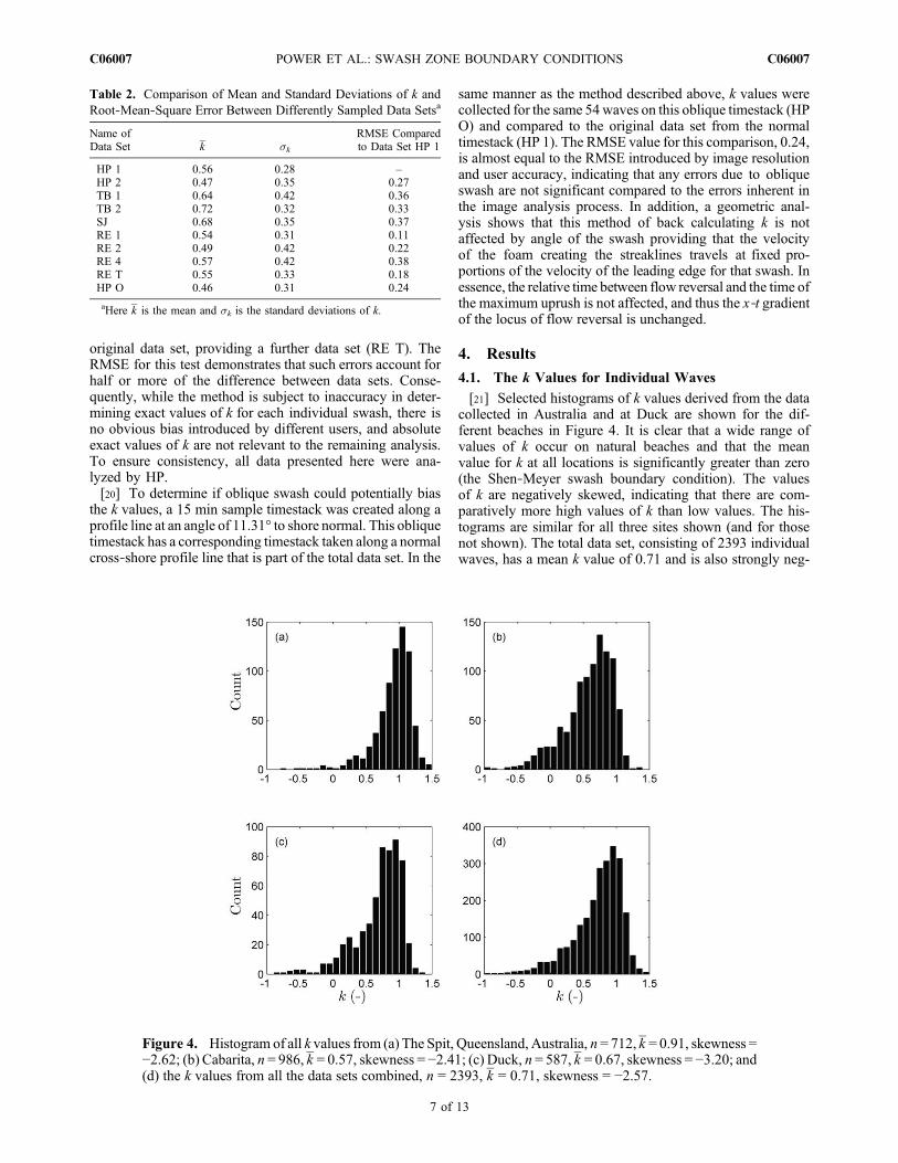
[21] Selected histograms of k values derived from the datacollected in Australia and at Duck are shown for the dif-ferent beaches in Figure 4. It is clear that a wide range ofvalues of k occur on natural beaches and that the meanvalue for k at all locations is significantly greater than zero(the Shen‐Meyer swash boundary condition). The valuesof k are negatively skewed, indicating that there are com-paratively more high values of k than low values. The his-tograms are similar for all three sites shown (and for thosenot shown). The total data set, consisting of 2393 individualwaves, has a mean k value of 0.71 and is also strongly neg-

Table 2. Comparison of Mean and Standard Deviations of k andRoot‐Mean‐Square Error Between Differently Sampled Data Setsa

Name ofData Set k sk

RMSE Comparedto Data Set HP 1

HP 1 0.56 0.28 –HP 2 0.47 0.35 0.27TB 1 0.64 0.42 0.36TB 2 0.72 0.32 0.33SJ 0.68 0.35 0.37RE 1 0.54 0.31 0.11RE 2 0.49 0.42 0.22RE 4 0.57 0.42 0.38RE T 0.55 0.33 0.18HP O 0.46 0.31 0.24

aHere k is the mean and sk is the standard deviations of k.

Figure 4. Histogram of all k values from (a) The Spit, Queensland, Australia, n = 712, k = 0.91, skewness =−2.62; (b) Cabarita, n = 986, k = 0.57, skewness = −2.41; (c) Duck, n = 587, k = 0.67, skewness = −3.20; and(d) the k values from all the data sets combined, n = 2393, k = 0.71, skewness = −2.57.

POWER ET AL.: SWASH ZONE BOUNDARY CONDITIONS C06007C06007

7 of 13

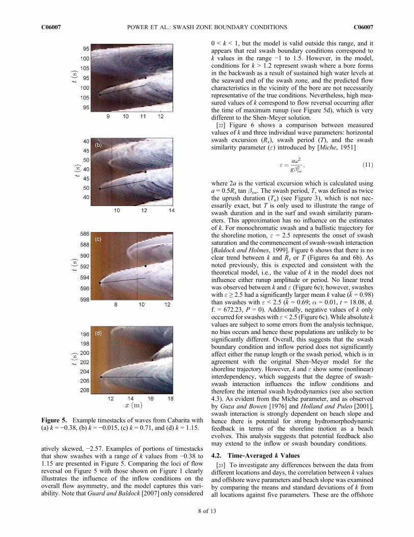
atively skewed, −2.57. Examples of portions of timestacksthat show swashes with a range of k values from −0.38 to1.15 are presented in Figure 5. Comparing the loci of flowreversal on Figure 5 with those shown on Figure 1 clearlyillustrates the influence of the inflow conditions on theoverall flow asymmetry, and the model captures this vari-ability. Note that Guard and Baldock [2007] only considered

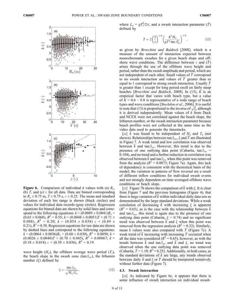
0 < k < 1, but the model is valid outside this range, and itappears that real swash boundary conditions correspond tok values in the range −1 to 1.5. However, in the model,conditions for k > 1.2 represent swash where a bore formsin the backwash as a result of sustained high water levels atthe seaward end of the swash zone, and the predicted flowcharacteristics in the vicinity of the bore are not necessarilyrepresentative of the true conditions. Nevertheless, high mea-sured values of k correspond to flow reversal occurring afterthe time of maximum runup (see Figure 5d), which is verydifferent to the Shen‐Meyer solution.[22] Figure 6 shows a comparison between measured

values of k and three individual wave parameters: horizontalswash excursion (Rx), swash period (T), and the swashsimilarity parameter (") introduced by [Miche, 1951]

" ¼ a!2

g�2sw

; ð11Þ

where 2a is the vertical excursion which is calculated usinga = 0.5Rx tan bsw. The swash period, T, was defined as twicethe uprush duration (Tu) (see Figure 3), which is not nec-essarily exact, but T is only used to illustrate the range ofswash duration and in the surf and swash similarity param-eters. This approximation has no influence on the estimatesof k. For monochromatic swash and a ballistic trajectory forthe shoreline motion, " = 2.5 represents the onset of swashsaturation and the commencement of swash‐swash interaction[Baldock and Holmes, 1999]. Figure 6 shows that there is noclear trend between k and Rx or T (Figures 6a and 6b). Asnoted previously, this is expected and consistent with thetheoretical model, i.e., the value of k in the model does notinfluence either runup amplitude or period. No linear trendwas observed between k and " (Figure 6c); however, swasheswith " ≥ 2.5 had a significantly larger mean k value (k = 0.98)than swashes with " < 2.5 (k = 0.69; a = 0.01, t = 18.08, d.f. = 672.23, P = 0). Additionally, negative values of k onlyoccurred for swashes with " < 2.5 (Figure 6c).While absolute kvalues are subject to some errors from the analysis technique,no bias occurs and hence these populations are unlikely to besignificantly different. Overall, this suggests that the swashboundary condition and inflow period does not significantlyaffect either the runup length or the swash period, which is inagreement with the original Shen‐Meyer model for theshoreline trajectory. However, k and " show some (nonlinear)interdependency, which suggests that the degree of swash‐swash interaction influences the inflow conditions andtherefore the internal swash hydrodynamics (see also section4.3). As evident from the Miche parameter, and as observedby Guza and Bowen [1976] and Holland and Puleo [2001],swash interaction is strongly dependent on beach slope andhence there is potential for strong hydromorphodynamicfeedback in terms of the shoreline motion as a beachevolves. This analysis suggests that potential feedback alsomay extend to the inflow or swash boundary conditions.

4.2. Time‐Averaged k Values

[23] To investigate any differences between the data fromdifferent locations and days, the correlation between k valuesand offshore wave parameters and beach slope was examinedby comparing the means and standard deviations of k fromall locations against five parameters. These are the offshore

Figure 5. Example timestacks of waves from Cabarita with(a) k = −0.38, (b) k = −0.015, (c) k = 0.71, and (d) k = 1.15.

POWER ET AL.: SWASH ZONE BOUNDARY CONDITIONS C06007C06007

8 of 13

wave height (Ho), the offshore average wave period (Tz),the beach slope in the swash zone (tanbsw), the Iribarrennumber (x) defined by

� ¼ tan �swffiffiffiffiffiffiffiffiffiffiffiffiffiHo=Lo

p ; ð12Þ

where Lo = gTz2/2p, and a swash interaction parameter (T̂ )

defined by

T̂ ¼ 22

�

� �1=4 K2Ho

gT 2 tan �2sw

� �1=4

; ð13Þ

as given by Brocchini and Baldock [2008], which is ameasure of the amount of interaction expected betweenmonochromatic swashes for a given beach slope and off-shore wave conditions. The difference between " and (T̂ )arises through the use of the offshore wave height andperiod, rather than the swash amplitude and period, which arenot independent of each other. Small values of T̂ correspondto no swash interaction and values of T̂ greater than orequal to 1 correspond to strong swash interaction. Usually T̂is greater than 1 except for long period swell on fairly steepbeaches [Brocchini and Baldock, 2008]. In (13), K is anempirical factor that varies with beach type, but a valueof K ≈ 0.6 − 0.8 is representative of a wide range of beachtypes and wave conditions [Stockdon et al., 2006]. It is usefulto note that (13) is proportional to the inverse of

ffiffiffi�

p, although

it is derived independently. Mean values of k from Duckand NCEX were not correlated against the beach slope, theIribarren number, or the swash interaction parameter becausebeach profiles were not collected at the same time as thevideo data used to generate the timestacks.[24] k was found to be independent of Ho and Tz (not

shown). Relationships between tanbsw, x and T̂ are illustratedin Figure 7. A weak trend and low correlation was observedbetween k and tanbsw. However, this trend is due to thepresence of one outlying data point (Cabarita, tanbsw =0.104), and no trend and a further reduction in correlation wasobserved between k and tanbswwhen this point was removedfrom the analysis (R2 = 0.0073; Figure 7a). Again, this lackof dependency is consistent with the theoretical basis of themodel; the variation in patterns of flow reversal are a resultof different inflow conditions for individual swash eventsand not strongly dependent on time‐averaged offshore waveconditions or beach slope.[25] Figure 7b shows the comparison of k with x. It is clear

from Figure 7 and the previous histograms (Figure 4), thatthere is large variation of k within individual daily data sets asdemonstrated by the large standard deviations. While a weakcorrelation of decreasing k with increasing x is apparent(R2 = 0.65), as is the case with the relationship between kand tanbsw, this trend is again due to the presence of oneoutlying data point (Cabarita, x = 0.74) and no significanttrend was observed between k and x when this point wasremoved from the regression analysis (R2 = 0.32). Similarly,mean k values were also compared with T̂ (Figure 7c). Aweak trend of k increasing with increasing T̂ occurred whenall the data was considered (R2 = 0.65), however, as with thetrends between k and tanbsw and k and x, no trend wasobserved when the one outlying data point was removed(Cabarita, T̂ = 1.10; R2 = 0.25). Additionally, in both cases, asthe standard deviations of k are large, any trends observedbetween daily k and x or T̂ should be interpreted tentativelywithout further data (Figure 7).

4.3. Swash Interaction

[26] As indicated by Figure 6c, it appears that there issome influence of swash interaction on individual swash‐

Figure 6. Comparison of individual k values with (a) Rx,(b) T, and (c) " for all data. Data are binned correspondingto Rx ± 0.75 m, T ± 0.75 s, " ± 0.25. The mean and standarddeviation of each bin range is shown (black circles) andvalues for individual data records (gray circles). Regressionequations for binned data are shown by solid lines and corre-spond to the following equations: k = (0.0089 ± 0.0041)Rx +(0.65 ± 0.068), R2 = 0.55; k = (0.0048 ± 0.0051)T + (0.71 ±0.088), R2 = 0.20; k = (0.054 ± 0.038) " + (0.69 ±0.21), R2 = 0.38. Regression equations for raw data are shownby dashed lines and correspond to the following equations:k = (0.0064 ± 0.0036)Rx + (0.68 ± 0.030), R2 = 0.0050; k =(0.0026 ± 0.0040)T + (0.70 ± 0.045), R2 = 0.00067; k =(0.18 ± 0.018) " + (0.39 ± 0.036), R2 = 0.19.

POWER ET AL.: SWASH ZONE BOUNDARY CONDITIONS C06007C06007

9 of 13

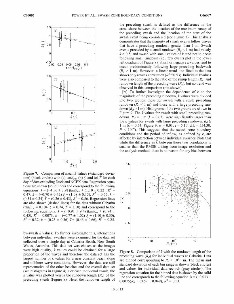
by‐swash k values. To further investigate this, interactionsbetween individual swashes were examined for the data setcollected over a single day at Cabarita Beach, New SouthWales, Australia. This data set was chosen as the imageswere high quality, k values could be obtained for a largeproportion of the waves and therefore the data set has thelargest number of k values for a near constant beach slopeand offshore wave conditions. However, the data are stillrepresentative of the other beaches and the overall data set(see histograms in Figure 4). For each individual swash, thek value was plotted versus the rundown length (Rd) of thepreceding swash (Figure 8). Here, the rundown length of

the preceding swash is defined as the difference in thecross shore between the location of the maximum runup ofthe preceding swash and the location of the start of theswash event being considered (see Figure 3). This analysisdemonstrates that the majority of swash events follow wavesthat have a preceding rundown greater than 1 m. Swashevents preceded by a small rundown (Rd < 1 m) had mostlyk > 0.5, and swash with small values of k tend not to occurfollowing small rundown (i.e., few events plot in the lowerleft quadrant of Figure 8). Small or negative k values tend tooccur predominantly following large preceding backwash(Rd > 1 m). However, a linear trend line fitted to the datashows only aweak correlation (R2 = 0.53). Individual k valueswere also compared to the ratio of the runup length (Rx) andrundown length of the preceding wave (Rd), but no trend wasobserved in this comparison (not shown).[27] To further investigate the dependence of k on the

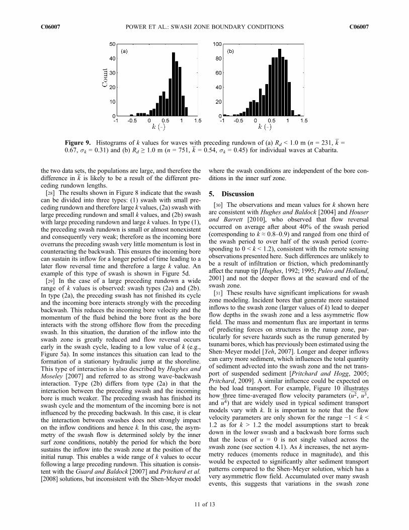
magnitude of the preceding rundown, k values were dividedinto two groups: those for swash with a small precedingrundown (Rd < 1 m) and those with a large preceding run-down (Rd > 1 m). Histograms of the two groups are shown inFigure 9. The k values for swash with small preceding run-downs, Rd < 1 m (k = 0.67), were significantly larger thanthe k values for swash with large preceding rundown, Rd ≥1 m (k = 0.54; Figure 9; a = 0.01; t = 5.10; d.f. = 554.30,P < 10−6). This suggests that the swash zone boundaryconditions and the period of inflow, as defined by k, areaffected by interaction between individual swashes. Note thatwhile the difference in k between these two populations issmaller than the RMSE arising from image resolution andthe analysis method, there is no reason for any bias between

Figure 8. Comparison of k with the rundown length of thepreceding wave (Rd) for individual waves at Cabarita. Dataare binned corresponding to Rd ± 100.1 m. The mean andstandard deviation of each bin range is shown (black circles)and values for individual data records (gray circles). Theregression equation for the binned data is shown by the solidline and corresponds to the following equation: k = (−0.013 ±0.0075)Rd + (0.69 ± 0.049), R2 = 0.53.

Figure 7. Comparison of mean k values (±standard devia-tion) (black circles) with (a) tanbsw, (b) x, and (c) T̂ for eachday of data excluding Duck and NCEX data. Regression equa-tions are shown (solid lines) and correspond to the followingequations: k = (−4.56 ± 3.91)tanbsw + (1.10 ± 0.22), R2 =0.47; k = (−0.70 ± 0.42) x + (1.08 ± 0.15), R2 = 0.65; k =(0.34 ± 0.24) T̂ + (0.26 ± 0.43), R2 = 0.56. Regression linesare also shown (dashed lines) for the data without Cabarita(tanbsw = 0.104, x = 0.74, T̂ = 1.10) and correspond to thefollowing equations: k = (−0.91 ± 9.49)tanbsw + (0.94 ±0.45), R2 = 0.0073; k = (−0.77 ± 1.02) x + (1.10 ± 0.30),R2 = 0.32; k = (0.23 ± 0.36) T̂+ (0.46 ± 0.66), R2 = 0.25.

POWER ET AL.: SWASH ZONE BOUNDARY CONDITIONS C06007C06007

10 of 13

the two data sets, the populations are large, and therefore thedifference in k is likely to be a result of the different pre-ceding rundown lengths.[28] The results shown in Figure 8 indicate that the swash

can be divided into three types: (1) swash with small pre-ceding rundown and therefore large k values, (2a) swash withlarge preceding rundown and small k values, and (2b) swashwith large preceding rundown and large k values. In type (1),the preceding swash rundown is small or almost nonexistentand consequently very weak; therefore as the incoming boreoverruns the preceding swash very little momentum is lost incounteracting the backwash. This ensures the incoming borecan sustain its inflow for a longer period of time leading to alater flow reversal time and therefore a large k value. Anexample of this type of swash is shown in Figure 5d.[29] In the case of a large preceding rundown a wide

range of k values is observed: swash types (2a) and (2b).In type (2a), the preceding swash has not finished its cycleand the incoming bore interacts strongly with the precedingbackwash. This reduces the incoming bore velocity and themomentum of the fluid behind the bore front as the boreinteracts with the strong offshore flow from the precedingswash. In this situation, the duration of the inflow into theswash zone is greatly reduced and flow reversal occursearly in the swash cycle, leading to a low value of k (e.g.,Figure 5a). In some instances this situation can lead to theformation of a stationary hydraulic jump at the shoreline.This type of interaction is also described by Hughes andMoseley [2007] and referred to as strong wave‐backwashinteraction. Type (2b) differs from type (2a) in that theinteraction between the preceding swash and the incomingbore is much weaker. The preceding swash has finished itsswash cycle and the momentum of the incoming bore is notinfluenced by the preceding backwash. In this case, it is clearthe interaction between swashes does not strongly impacton the inflow conditions and hence k. In this case, the asym-metry of the swash flow is determined solely by the innersurf zone conditions, notably the period for which the boresustains the inflow into the swash zone at the position of theinitial runup. This enables a wide range of k values to occurfollowing a large preceding rundown. This situation is consis-tent with the Guard and Baldock [2007] and Pritchard et al.[2008] solutions, but inconsistent with the Shen‐Meyer model

where the swash conditions are independent of the bore con-ditions in the inner surf zone.

5. Discussion

[30] The observations and mean values for k shown hereare consistent with Hughes and Baldock [2004] and Houserand Barrett [2010], who observed that flow reversaloccurred on average after about 40% of the swash period(corresponding to k ≈ 0.8–0.9) and ranged from one third ofthe swash period to over half of the swash period (corre-sponding to 0 < k < 1.2), consistent with the remote sensingobservations presented here. Such differences are unlikely tobe a result of infiltration or friction, which predominantlyaffect the runup tip [Hughes, 1992; 1995; Puleo and Holland,2001] and not the deeper flows at the seaward end of theswash zone.[31] These results have significant implications for swash

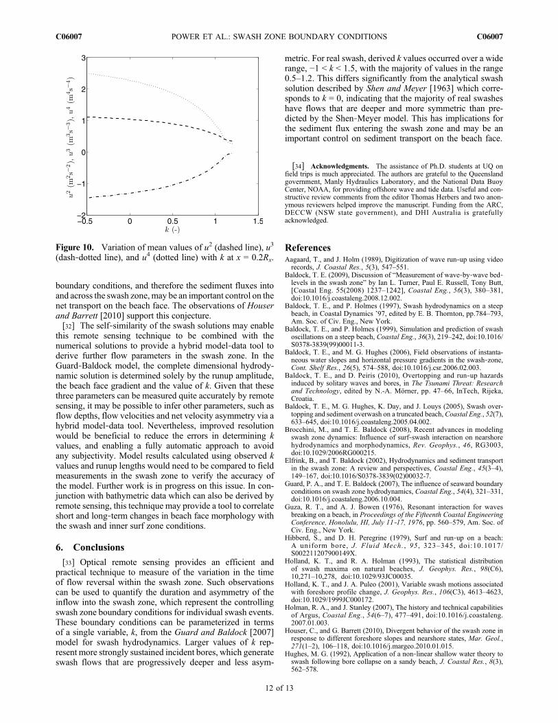
zone modeling. Incident bores that generate more sustainedinflows to the swash zone (larger values of k) lead to deeperflow depths in the swash zone and a less asymmetric flowfield. The mass and momentum flux are important in termsof predicting forces on structures in the runup zone, par-ticularly for severe hazards such as the runup generated bytsunami bores, which has previously been estimated using theShen‐Meyer model [Yeh, 2007]. Longer and deeper inflowscan carry more sediment, which influences the total quantityof sediment advected into the swash zone and the net trans-port of suspended sediment [Pritchard and Hogg, 2005;Pritchard, 2009]. A similar influence could be expected onthe bed load transport. For example, Figure 10 illustrateshow three time‐averaged flow velocity parameters (u2, u3,and u4) that are widely used in typical sediment transportmodels vary with k. It is important to note that the flowvelocity parameters are only shown for the range −1 < k <1.2 as for k > 1.2 the model assumptions start to breakdown in the lower swash and a backwash bore forms suchthat the locus of u = 0 is not single valued across theswash zone (see section 4.1). As k increases, the net asym-metry reduces (moments reduce in magnitude), and thiswould be expected to significantly alter sediment transportpatterns compared to the Shen‐Meyer solution, which has avery asymmetric flow field. Accumulated over many swashevents, this suggests that variations in the swash zone

Figure 9. Histograms of k values for waves with preceding rundown of (a) Rd < 1.0 m (n = 231, k =0.67, sk = 0.31) and (b) Rd ≥ 1.0 m (n = 751, k = 0.54, sk = 0.45) for individual waves at Cabarita.

POWER ET AL.: SWASH ZONE BOUNDARY CONDITIONS C06007C06007

11 of 13

boundary conditions, and therefore the sediment fluxes intoand across the swash zone, may be an important control on thenet transport on the beach face. The observations of Houserand Barrett [2010] support this conjecture.[32] The self‐similarity of the swash solutions may enable

this remote sensing technique to be combined with thenumerical solutions to provide a hybrid model‐data tool toderive further flow parameters in the swash zone. In theGuard‐Baldock model, the complete dimensional hydrody-namic solution is determined solely by the runup amplitude,the beach face gradient and the value of k. Given that thesethree parameters can be measured quite accurately by remotesensing, it may be possible to infer other parameters, such asflow depths, flow velocities and net velocity asymmetry via ahybrid model‐data tool. Nevertheless, improved resolutionwould be beneficial to reduce the errors in determining kvalues, and enabling a fully automatic approach to avoidany subjectivity. Model results calculated using observed kvalues and runup lengths would need to be compared to fieldmeasurements in the swash zone to verify the accuracy ofthe model. Further work is in progress on this issue. In con-junction with bathymetric data which can also be derived byremote sensing, this technique may provide a tool to correlateshort and long‐term changes in beach face morphology withthe swash and inner surf zone conditions.

6. Conclusions

[33] Optical remote sensing provides an efficient andpractical technique to measure of the variation in the timeof flow reversal within the swash zone. Such observationscan be used to quantify the duration and asymmetry of theinflow into the swash zone, which represent the controllingswash zone boundary conditions for individual swash events.These boundary conditions can be parameterized in termsof a single variable, k, from the Guard and Baldock [2007]model for swash hydrodynamics. Larger values of k rep-resent more strongly sustained incident bores, which generateswash flows that are progressively deeper and less asym-

metric. For real swash, derived k values occurred over a widerange, −1 < k < 1.5, with the majority of values in the range0.5–1.2. This differs significantly from the analytical swashsolution described by Shen and Meyer [1963] which corre-sponds to k = 0, indicating that the majority of real swasheshave flows that are deeper and more symmetric than pre-dicted by the Shen‐Meyer model. This has implications forthe sediment flux entering the swash zone and may be animportant control on sediment transport on the beach face.

[34] Acknowledgments. The assistance of Ph.D. students at UQ onfield trips is much appreciated. The authors are grateful to the Queenslandgovernment, Manly Hydraulics Laboratory, and the National Data BuoyCenter, NOAA, for providing offshore wave and tide data. Useful and con-structive review comments from the editor Thomas Herbers and two anon-ymous reviewers helped improve the manuscript. Funding from the ARC,DECCW (NSW state government), and DHI Australia is gratefullyacknowledged.

ReferencesAagaard, T., and J. Holm (1989), Digitization of wave run‐up using videorecords, J. Coastal Res., 5(3), 547–551.

Baldock, T. E. (2009), Discussion of “Measurement of wave‐by‐wave bed‐levels in the swash zone” by Ian L. Turner, Paul E. Russell, Tony Butt,[Coastal Eng. 55(2008) 1237–1242], Coastal Eng., 56(3), 380–381,doi:10.1016/j.coastaleng.2008.12.002.

Baldock, T. E., and P. Holmes (1997), Swash hydrodynamics on a steepbeach, in Coastal Dynamics ’97, edited by E. B. Thornton, pp.784–793,Am. Soc. of Civ. Eng., New York.

Baldock, T. E., and P. Holmes (1999), Simulation and prediction of swashoscillations on a steep beach, Coastal Eng., 36(3), 219–242, doi:10.1016/S0378-3839(99)00011-3.

Baldock, T. E., and M. G. Hughes (2006), Field observations of instanta-neous water slopes and horizontal pressure gradients in the swash‐zone,Cont. Shelf Res., 26(5), 574–588, doi:10.1016/j.csr.2006.02.003.

Baldock, T. E., and D. Peiris (2010), Overtopping and run‐up hazardsinduced by solitary waves and bores, in The Tsunami Threat: Researchand Technology, edited by N.-A. Mörner, pp. 47–66, InTech, Rijeka,Croatia.

Baldock, T. E., M. G. Hughes, K. Day, and J. Louys (2005), Swash over-topping and sediment overwash on a truncated beach,Coastal Eng., 52(7),633–645, doi:10.1016/j.coastaleng.2005.04.002.

Brocchini, M., and T. E. Baldock (2008), Recent advances in modelingswash zone dynamics: Influence of surf‐swash interaction on nearshorehydrodynamics and morphodynamics, Rev. Geophys., 46, RG3003,doi:10.1029/2006RG000215.

Elfrink, B., and T. Baldock (2002), Hydrodynamics and sediment transportin the swash zone: A review and perspectives, Coastal Eng., 45(3–4),149–167, doi:10.1016/S0378-3839(02)00032-7.

Guard, P. A., and T. E. Baldock (2007), The influence of seaward boundaryconditions on swash zone hydrodynamics, Coastal Eng., 54(4), 321–331,doi:10.1016/j.coastaleng.2006.10.004.

Guza, R. T., and A. J. Bowen (1976), Resonant interaction for wavesbreaking on a beach, in Proceedings of the Fifteenth Coastal EngineeringConference, Honolulu, HI, July 11‐17, 1976, pp. 560–579, Am. Soc. ofCiv. Eng., New York.

Hibberd, S., and D. H. Peregrine (1979), Surf and run‐up on a beach:A uniform bore, J. Fluid Mech. , 95 , 323–345, doi:10.1017/S002211207900149X.

Holland, K. T., and R. A. Holman (1993), The statistical distributionof swash maxima on natural beaches, J. Geophys. Res., 98(C6),10,271–10,278, doi:10.1029/93JC00035.

Holland, K. T., and J. A. Puleo (2001), Variable swash motions associatedwith foreshore profile change, J. Geophys. Res., 106(C3), 4613–4623,doi:10.1029/1999JC000172.

Holman, R. A., and J. Stanley (2007), The history and technical capabilitiesof Argus, Coastal Eng., 54(6–7), 477–491, doi:10.1016/j.coastaleng.2007.01.003.

Houser, C., and G. Barrett (2010), Divergent behavior of the swash zone inresponse to different foreshore slopes and nearshore states, Mar. Geol.,271(1–2), 106–118, doi:10.1016/j.margeo.2010.01.015.

Hughes, M. G. (1992), Application of a non‐linear shallow water theory toswash following bore collapse on a sandy beach, J. Coastal Res., 8(3),562–578.

Figure 10. Variation of mean values of u2 (dashed line), u3

(dash‐dotted line), and u4 (dotted line) with k at x = 0.2Rx.

POWER ET AL.: SWASH ZONE BOUNDARY CONDITIONS C06007C06007

12 of 13

Hughes, M. G. (1995), Friction factors for wave uprush, J. Coastal Res.,11(4), 1089–1098.

Hughes, M. G., and T. E. Baldock (2004), Eulerian flow velocities in theswash zone: Field data and model predictions, J. Geophys. Res., 109,C08009, doi:10.1029/2003JC002213.

Hughes, M. G., and A. S. Moseley (2007), Hydrokinematic regions withinthe swash zone, Cont. Shelf Res., 27(15), 2000–2013, doi:10.1016/j.csr.2007.04.005.

Hughes, M. G., G. Masselink, and R. W. Brander (1997), Flow velocityand sediment transport in the swash zone of a steep beach, Mar. Geol.,138(1–2), 91–103, doi:10.1016/S0025-3227(97)00014-5.

Kemp, P. H. (1975), Wave asymmetry in the nearshore zone and breakerarea, in Nearshore Sediment Dynamics and Sedimentation, edited byJ. Hail and A. Carr, pp. 47–67, John Wiley, Hoboken, N. J.

Kobayashi, N., G. S. DeSilva, and K. D. Watson (1989), Wave transforma-tion and swash oscillation on gentle and steep slopes, J. Geophys. Res.,94(C1), 951–966, doi:10.1029/JC094iC01p00951.

Larson, M., and N. C. Kraus (1994), Temporal and spatial scales of beachprofile change, Duck, North Carolina, Mar. Geol., 117(1–4), 75–94,doi:10.1016/0025-3227(94)90007-8.

Lippmann, T. C., and R. A. Holman (1989), Quantification of sand barmorphology: A video technique based on wave dissipation, J. Geophys.Res., 94(C1), 995–1011, doi:10.1029/JC094iC01p00995.

Masselink, G., and M. Hughes (1998), Field investigation of sedimenttransport in the swash zone, Cont. Shelf Res., 18(10), 1179–1199,doi:10.1016/S0278-4343(98)00027-2.

Masselink, G., and J. A. Puleo (2006), Swash‐zone morphodynamics,Cont. Shelf Res., 26(5), 661–680, doi:10.1016/j.csr.2006.01.015.

Miche, R. (1951), Le pouvoir réfléchissant des ouvrages maritimes exposésà l’action de la houle, Ann. Ponts Chaussees, 121, 285–319.

Packwood, A. R. (1983), The influence of beach porosity on wave uprushand backwash, Coastal Eng., 7(1), 29–40, doi:10.106/0378-3839(83)90025-X.

Peregrine, D. H., and S. M. Williams (2001), Swash overtopping a trun-cated plane beach, J. Fluid Mech., 440, 391–399, doi:10.1017/S002211200100492X.

Power, H. E., M. Palmsten, R. A. Holman, and T. E. Baldock (2009),Remote sensing of swash zone boundary conditions using videoand ARGUS, in Proceedings of Coastal Dynamics 2009, edited byM. Mizuguchi and S. Sato, pp. 1–11, Am. Soc. of Civ. Eng., New York.

Pritchard, D. (2009), Sediment transport under a swash event: The effectof boundary conditions, Coastal Eng., 56(9), 970–981, doi:10.1016/j.coastaleng.2009.06.004.

Pritchard, D., and A. J. Hogg (2005), On the transport of suspended sedi-ment by a swash event on a plane beach, Coastal Eng., 52(1), 1–23,doi:10.1016/j.coastaleng.2004.08.002.

Pritchard, D., P. A. Guard, and T. E. Baldock (2008), An analytical modelfor bore‐driven run‐up, J. Fluid Mech., 610, 183–193.

Puleo, J. A., and K. T. Holland (2001), Estimating swash zone friction coef-ficients on a sandy beach,Coastal Eng., 43(1), 25–40, doi:10.1016/S0378-3839(01)00004-7.

Puleo, J. A., R. A. Beach, R. A. Holman, and J. S. Allen (2000), Swashzone sediment suspension and transport and the importance of bore‐generated turbulence, J. Geophys. Res., 105(C7), 17,021–17,044,doi:10.1029/2000JC900024.

Puleo, J. A., K. T. Holland, N. G. Plant, D. N. Slinn, and D. M. Hanes(2003), Fluid acceleration effects on suspended sediment transport inthe swash zone, J. Geophys. Res., 108(C11), 3350, doi:10.1029/2003JC001943.

Ranasinghe, R., G. Symonds, K. Black, and R. A. Holman (2004), Morpho-dynamics of intermediate beaches: A video imaging and numericalmodelling study, Coastal Eng., 51(7), 629–655, doi:10.1016/j.coastaleng.2004.07.018.

Raubenheimer, B. (2002), Observations and predictions of fluid velocitiesin the surf and swash zone, J. Geophys. Res., 107(C11), 3190,doi:10.1029/2001JC001264.

Raubenheimer, B., R. T. Guza, S. Elgar, and N. Kobayashi (1995), Swashon a gently sloping beach, J. Geophys. Res., 100(C5), 8751–8760,doi:10.1029/95JC00232.

Shen, M. C., and R. E. Meyer (1963), Climb of a bore on a beach Part 3.Run‐up, J. Fluid Mech., 16, 113–125, doi:10.1017/S0022112063000628.

Stockdon, H. F., and R. A. Holman (2000), Estimation of wave phase speedand nearshore bathymetry from video imagery, J. Geophys. Res., 105(C9),22,015–22,033, doi:10.1029/1999JC000124.

Stockdon, H. F., R. A. Holman, P. A. Howd, and A. H. Sallenger (2006),Empirical parameterization of setup, swash, and runup, Coastal Eng.,53(7), 573–588, doi:10.1016/j.coastaleng.2005.12.005.

Turner, I. L., P. E. Russell, T. Butt, C. E. Blenkinsopp, and G. Masselink(2009), In‐situ estimates of net sediment flux per swash: Reply to dis-cussion by TE Baldock of “Measurement of wave‐by‐wave bed‐levelsin the swash zone”, Coastal Eng., 56(9), 1009–1012, doi:10.1016/j.coastaleng.2009.06.001.

Waddell, E. (1976), Swash‐groundwater‐beach profile interactions, inBeach and Nearshore Sediment, Spec. Publ. Ser., vol. 24, edited byR.A. Davis andR.L. Etherington, pp. 115–125, Soc. of Econ. and Paleontol.Mineral., Tulsa, Okla.

Wright, L. D., and A. D. Short (1984), Morphodynamic variability of surfzones and beaches: A synthesis, Mar. Geol., 56(1–4), 93–118,doi:10.1016/0025-3227(84)90008-2.

Yeh, H. (2007), Design tsunami forces for onshore structures, J. DisasterRes., 2(6), 531–536.

T. E. Baldock and H. E. Power, School of Civil Engineering, Universityof Queensland, Level 3, Room C312, Hawken Engineering Building,St Lucia, Qld 4072, Australia. (h.power@uq.edu.au)R. A. Holman, College of Oceanic and Atmospheric Sciences, Oregon

State University, 104 COAS Administration Bldg., Corvallis, OR 97331,USA.

POWER ET AL.: SWASH ZONE BOUNDARY CONDITIONS C06007C06007

13 of 13