arX

iv:g

r-qc

/950

3013

v1 7

Mar

199

5

On estimation of the post-Newtonian parameters in the

gravitational-wave emission of a coalescing binary

Andrzej Krolak

Max-Planck-Research-Group Gravitational Theory

at the Friedrich-Schiller-University, 07743 Jena, Germany ∗

Kostas D. Kokkotas

Section Astrophysics, Astronomy and Mechanics,

Department of Physics, Aristotle University of Thessaloniki,

540 06 Thessaloniki, Macedonia, Greece

Gerhard Schafer

Max-Planck-Research-Group Gravitational Theory

at the Friedrich-Schiller-University, 07743 Jena, Germany

∗Permanent address: Institute of Mathematics, Polish Academy of Sciences, Sniadeckich 8, 00-950 Warsaw, Poland.

2

Abstract

The effect of the recently obtained 2nd post-Newtonian corrections on the accuracy of estimationof parameters of the gravitational-wave signal from a coalescing binary is investigated. It is shownthat addition of this correction degrades considerably the accuracy of determination of individualmasses of the members of the binary. However the chirp mass and the time parameter in the signalis still determined to a very good accuracy. The possibility of estimation of effects of other theoriesof gravity is investigated. The performance of the Newtonian filter is investigated and it is comparedwith performance of post-Newtonian search templates introduced recently. It is shown that bothsearch templates can extract accurately useful information about the binary.

PACS numbers: 04.30.+x,04.80.+x,95.85.5z,97.80.Af

3

1 Introduction

It is currently believed that the gravitational waves that come from the final stages of the evolution ofcompact binaries just before their coalescence are very likely signals to be detected by long-arm laserinterferometers [1]. The reason is that in the case of binary systems we can predict the gravitationalwaveform very well; and the amplitudes are reasonably high for sources at distances out to 200 Mpc.An estimate based on the number of compact binaries known in our galaxy and extrapolated to the restof the Universe shows that there should be one neutron star compact binary coalescence per year outto the distance of 200Mpc [2, 3]. This estimate is a safe lower bound on the rate of binary coalescence.Arguments based on progenitor evolution scenarios suggest that there should be 100 of two neutronstar coalescences, 5 neutron star - black hole coalescences, and 0.5 two black hole coalescences out to200Mpc [4]. The waveform derived using the quadrupole formula has been known for quite some time[5]. A standard optimal method to detect the signal from a coalescing binary in a noisy data set andto estimate its parameters is to correlate the data with the filter matched to the signal and vary theparameters of the filter until the correlation is maximal. The parameters of the filter that maximize thecorrelation are estimators for the parameters of the signal. The detailed algorithms and the performanceof the matched-filtering method in application to coalescing binary gravitational-wave signal has beeninvestigated by several authors, e.g. [6, 7, 8, 9, 10]. It has recently been realized [11] that the correlationis very sensitive even to very small variations of the phase of the filter because of the large numberof cycles in the signal. Consequently the addition of small corrections to the phase of the signal dueto the post-Newtonian effects decreases the correlation considerably. Thus the post-Newtonian effectsin the coalescing binary waveform can be detected and estimated to a much higher accuracy than itwas thought before [12]. This opens up new prospects but also considerable data analysis challengesfor the LIGO, VIRGO, and GEO600 projects which are rapidly progressing. It was also found [11]that the post-Newtonian series is not converging rapidly for a binary near coalescence. Hence higherpost-Newtonian corrections will affect the correlation. Currently three post-Newtonian corrections to thequadrupole formula are already known [13] and the calculation of further ones is in progress. In thisarticle we analyse the estimation of parameters of the 2nd post-Newtonian signal. This part of workcomplements a recent detailed analysis of the 3/2 post-Newtonian signal performed recently in Ref.[10].We also examine the detectability of the post-Newtonian signal and estimation of its parameters using theNewtonian waveform as a filter. This filter can be used as the simplest search template. We compare theNewtonian search templates with the post-Newtonian search templates recently investigated in Ref.[14].

The paper is organized as follows. In the first part of Section 2 we present the gravitational wave signalfrom a binary system to the currently known 2nd post-Newtonian order. In this work we analyse the signalin the “restricted” post-Newtonian approximation (i.e. only the phase of the signal is given to the 2ndpost-Newtonian accuracy whereas the amplitude of the signal is calculated from the quadrupole formula),we assume circularized orbits, and we assume the spin parameters to be constant. In the second part webriefly describe the optimal method of detection of such a signal in noise and the maximum likelihood(ML) method to estimate the parameters of the signal. We derive a number of properties of the MLestimators of the parameters of our signal and we examine the bounds on their variances. Our analysis isbased on the Cramer-Rao bound. In the third part we give the approximate rms errors of the estimatorsfor the signal at various post-Newtonian orders. In the fourth part of Section 2 we consider the effectsof other theories of gravity and their detectability from gravitational-wave measurements. We considerJordan-Fiertz-Brans-Dicke theory and Damour-Esposito-Farese biscalar tensor theory. In Section 3 weconsider the so called “search templates” introduced in Ref.[11]. These are simple filters containing asfew parameters as possible to effectively detect the multi-parameter signals. In the first part of Section 3we analyse the simplest search template - the Newtonian filter which is the waveform of the gravitationalsignal from a binary in the quadrupole approximation. We examine the Newtonian filter as a tool bothto detect the signal and also to determine its nature. In the second part of Section 3 we compare theNewtonian filter with the other search template analysed recently [14] based on the full post-Newtoniansignal. In Section 4 we summarize conclusions from our results. A number of results is left to appendices.In Appendix A we examine the first order effects on the phase of the signal due to eccentricity. InAppendix B we give numerical values of the covariance matrices at various post-Newtonian orders. InAppendix C we give certain detailed formulae for the Damour-Esposito-Farese theory. In Appendix Dwe briefly review the theory of optimal detection of known signal in noise and we generalize it to non-optimal detection. In Appendix E we give a useful analytic approximation to the correlation integral of

4

the optimal filter with the signal from a binary.

The units are chosen such that G = c = 1.

2 Post-Newtonian effects

2.1 Gravitational wave signal from a coalescing binary

Let us first give the formula for the gravitational waveform of a binary with the three currently knownpost-Newtonian corrections. We make the following approximations. We work within the so called“restricted” post-Newtonian approximation i.e. we only include the post-Newtonian corrections to thephase of the signal keeping the amplitude in its Newtonian form; this is because the effect of the phase onthe correlation is dominant. The inclusion of post-Newtonian effects in amplitudes will not qualitativelychange our results. Due to the effect of rapid circularization of the orbit by radiation reaction one canassume that the orbit is quasicircular. For example in the case of the gravitational wave signal from theHulse-Taylor binary pulsar at the characteristic frequency of the detector for such a signal of around 47Hzthe eccentricity e would be ∼ 10−6. Moreover the first order contribution to the phase of the signal due toeccentricity goes like e2. Nevertheless for completeness we include the first order correction to the signaldue to eccentricity in our formulae. We give a detailed derivation of this correction in Appendix A. Weneglect the tidal effects. All tidal contributions to the gravitational wave signal from a coalescing binarywere estimated to be small [12, 15]. There is also a small additional contribution to the phase due to taileffects which detectability has been considered in detail [16] and was found to be small. This correctionis formally of the 4th post-Newtonian order and consequently we neglect it in the present analysis.

With these approximations the waveform, as a function of time, is given by the following expression,

h(t) = Af(t)2/3 cos[2π

∫ t

ta

f(t′)dt′ − φ], (1)

where

A =8

5π2/3 µm2/3

R(2)

and where φ is an arbitrary phase, µ and m are the reduced and the total mass of the binary, respectively;ta is a time parameter and R is the distance to the source. A is the rms average amplitude over all Eulerangles determining the position of the binary on the sky and the inclination angle between the plane of theorbit of the binary and the line of sight. The rms amplitude A is 2/5 of the maximum possible amplitude.The characteristic time for the evolution of the binary to the currently known 2nd post-Newtonian orderis given by

τ2PN :=f

df/dt=

5

96

1

µm2/3

1

(πf)8/3× (3)

[1 − 157

24

Ie

f19/9+ (

743

336+

11

4

µ

m)(πmf)2/3 − (4π − so)(πmf) + (4)

(3058673

1016064+

5429

1008

µ

m+

617

144(µ

m)2 + ss

m

µ)(πmf)4/3]

where Ie is the asymptotic eccentricity invariant,

Ie = e20f

19/9

0 , (5)

e0 is the eccentricity of the binary at gravitational frequency f0 (see Appendix A for derivation andexplanations). The quantities so and ss are spin-orbit and spin-spin parameters respectively. They aregiven by the formula

so =113

12(s1 + s2) +

25

4(s1

m2

m1

+ s2

m1

m2

) (6)

ss =247

48s1 · s2 − 721

48s1s2 (7)

5

s1 =S1

m2, s2 =

S2

m2(8)

s1 = L · s1, s2 = L · s2, (9)

where L is the total orbital angular momentum and S1, S2 are the spin angular momenta of the twobodies. The terms in square brackets in Eq.(4) are respectively: at lowest order, Newtonian (quadrupole);at order f−19/9, lowest order contribution due to eccentricity (see Appendix A); at order f2/3, 1PN [17];at order f , the non-linear effect of ”tails” of the wave (4π term) [18, 43, 35, 21]), and spin-orbit effects[22]; and at order f4/3, 2PN [13] and spin-spin effects [22].

In general the spin parameters vary with time. It was shown [10] that so is nearly conserved, it neverdeviates from its average value by more than ∼ 0.25. Moreover the time dependent part of the spinparameter is oscillatory what reduces considerably its influence on the phase of the signal [10]. In thiswork we shall assume that both spin-orbit and spin-spin parameters are constant. We also neglect theeffect of the precession of the orbital plane due to spin on the waveform. The effects of the spin on thewaveform of the signal from an inspiralling binary have been investigated in detail in [23]. If we take theavailable estimate of the moment of inertia for the pulsar in the Hulse-Taylor binary and assume massesof the neutron stars in the binary of 1.4 solar masses then so ≃ 4.8 × 10−2 and ss ≃ 2.4 × 10−5. If suchvalues are typical then spin effects will make negligible contributions to the phase of the signal. Howeverthis may not be the case for binaries containing black holes. Moreover if cosmic censorship is violated andblack holes rotate at a higher rate than allowed by maximally rotating Kerr black hole the spin effectswill significantly affect the gravitational waveform.

In the analysis of the detection of the above signal and estimation of its parameters it is convenient towork in the Fourier domain. The expression for the Fourier transform of our signal in the stationaryphase approximation is given by (cf.[1, 24, 6, 10])

h = Af−7/6 exp i[2πfta − φ − π/4 + (10)

5

48(a(f ; fa)k + ae(f ; fa)ke + a1(f ; fa)k1 + a3/2(f ; fa)k3/2 + a2(f ; fa)k2)],

for f > 0 and by the complex conjugate of the above expression for f < 0 where

A =1

(30)1/2

1

π2/3

µ1/2m1/3

R, (11)

k =1

µm2/3, (12)

ke =1

µm2/3e20(πf0)

19/9, (13)

k1 =1

µ(743

336+

11

4ν), (14)

k3/2 =m1/3

µ(4π − so), (15)

k2 =m4/3

µ

(

3058673

1016064+

5429

1008ν +

617

144ν2 +

ss

ν

)

, (16)

a(f ; fa) =9

40

1

(πf)5/3+

3

8

πf

(πfa)8/3− 3

5

1

(πfa)5/3, (17)

ae(f ; fa) = −157

24

(

81

1462

1

(πf)34/9+

9

43

πf

(πfa)43/9− 9

34

1

(πfa)34/9

)

, (18)

a1(f ; fa) =1

2

1

πf+

1

2

πf

(πfa)2− 1

πfa, (19)

a3/2(f ; fa) = −(

9

10

1

(πf)2/3+

3

5

πf

(πfa)5/3− 3

2

1

(πfa)2/3

)

, (20)

a2(f ; fa) =9

4

1

(πf)1/3+

3

4

πf

(πfa)4/3− 3

(πfa)1/3(21)

hold and where fa = f(ta).

6

The stationary phase approximation, Eq.(11), is an excellent approximation of the Fourier transform ofthe signal for frequencies which are not influenced by the finite time window of the measurement. In theabove expressions for the gravitational wave signal from a binary we can make an arbitrary choice of thetime parameter and the phase of the signal.

We also point out that going from the time to the frequency domain we have made yet another approxi-mation. Namely we have taken the modulus | h | of the Fourier transform to be the Newtonian one i.e.

| h |∼ f−7/6. In the stationary phase approximation | h | goes like 1/

√

f and consequently by Eq.(153)there would be other powers of frequency due to the post-Newtonian effects. We neglect those additionalterms since the post-Newtonian corrections to the phase have the dominant effect. The inclusion of thepost-Newtonian amplitudes to the signal will not qualitatively change the results of this work.

A convenient parameter is the chirp mass defined as M := k−3/5. In the quadrupole approximation thegravitational wave signal from a binary is entirely determined by the chirp mass.

We shall consider three models of binaries: neutron star/neutron star (NS-NS), neutron star/black hole(NS-BH), and black hole/black hole (BH-BH) binaries with parameters summarized in Table I.

Table I. Numerical values of the parameters of the three fiducial binary systems. Black holes are of 10solar masses and neutron stars are of 1.4 solar masses. Spin parameters are assumed to be constant.Spin for neutron stars was calculated from the typical estimate of the moment of inertia I for a neutronstar of I = 1038 kg m2.

A

Binary m1[M⊙] m2[M⊙] M[M⊙] s1 s2 so ss

1. NS-NS 1.4 1.4 1.2 1.5×10−3 1.5×10−3 4.8×10−2 2.4×10−5

2. NS-BH 1.4 10 3.0 3.0×10−5 0.38 4.0 3.5 ×10−4

3. BH-BH 10 10 8.7 0.13 0.13 3.9 0.15

B

Binary k[M−5/3

⊙ ] k1[M−1⊙ ] k3/2[M

−2/3

⊙ ] k2[M−1/3

⊙ ]1. NS-NS 0.72 4.1 25 132. NS-BH 0.16 2.0 16 153. BH-BH 2.7×10−2 0.58 4.7 7.7

where M⊙ means solar mass.

For neutron stars we calculated the spin using the available estimate of the moment of inertia for theneutron star in the binary pulsar PSR1916+19. We have taken black holes to be spinning at half themaximum rate (i.e. si = 0.5m2

i /m2). The orbital momenta vectors were assumed to be parallel to thespin vectors.

To have an idea of the size of the post-Newtonian corrections in the gravitational wave signal from a binarywhen it enters the observation window of the laser interferometer we have evaluated the characteristictime τ2PN for the above three models at the frequency f ′

o = 47 Hz which is the characteristic frequencyof the detector for this signal (see below). We have made explicit the contributions to the characteristictime from the three post-Newtonian corrections.

τ12PN = 44(1 + 0.046[from 1pn] − 0.025[from 3/2pn] + 0.0012[from 2pn])sec (22)

τ22PN = 9.9(1 + 0.10[from 1pn] − 0.071[from 3/2pn] + 0.0060[from 2pn])sec (23)

τ32PN = 1.7(1 + 0.17[from 1pn] − 0.12[from 3/2pn] + 0.018[from 2pn])sec (24)

One concludes from the above numbers that for the earth-based laser interferometers post-Newtoniancorrections are significant. Moreover several things are apparent. The quadrupole term is dominant forall the three models. This indicates a very good accuracy of the quadrupole formula even in the regimeof strongly gravitating bodies. This has been noticed in other studies for example in the numericalinvestigation of the gravitational wave emission from the two black hole collisions [44]. The difference

7

in size between the 1st post-Newtonian correction and the 3/2 post-Newtonian correction (tail term)is rather small. They differ by a factor of 2 for NS-NS binary and only by a factor of around 1.5 forbinaries with a black hole. The second post-Newtonian correction is noticably smaller then the 3/2 post-Newtonian correction. The difference varies form a factor of 20 for a NS-NS binary to a factor of 7 for aBH-BH binary. The convergence of the post-Newtonian series appears to be worst for BH-BH binariesand in this case it would be desirable to have accurate numerical waveforms and not only the ones basedon the post-Newtonian approximation. Such waveforms should be available as a result of the numericalprojects such as Grand Challenge project currently under way in the United States.

2.2 Detection of the signal and estimation of its parameters

For the purpose of this investigation we shall use a fit to the total spectral density Sh(f) of the noise inthe advanced LIGO detectors, devised in [10]. This fit comprises seismic, thermal, shot, and quantumnoises in the detector.

Sh(f) = So((fo/f)4 + 2(1 + (f/fo)2))/5, (25)

where fo = 70Hz and So = 3 × 10−48Hz−1. It is an excellent approximation to the detailed formulaefor various noises given in [6]. The sensitivity function Sen(f) of the detector is defined as 1/Sh(f).The sensitivity function has the maximum at frequency fo given above and its half width half magnitude(HWHM) σo is around 48Hz.

To determine whether or not there is a signal in a noisy data set we use the Neyman-Pearson test (seeAppendix D). When the noise in the detector is Gaussian the Neyman-Pearson test is the correlator test.It consists of linear filtering the data with the filter which Fourier transform is the Fourier transformof the signal divided by the spectral density of the noise [26]. The signal-to-noise ratio d that can beachieved by optimal filtering is given by d = (h|h)1/2 where following [10] the scalar product (h1|h2) isdefined by

(h1|h2) = 4ℜ∫ ∞

fi

h∗1h2

Sh(f)df, (26)

where ℜ denotes the real part. Thus we have

d2 = 4A2

∫ ∞

fi

df

Sh(f)f7/3. (27)

We shall call the integrand of the above signal-to-noise integral signal sensitivity function and we denoteit by Ind(f). This function has the maximum at the frequency f ′

o where f ′o = 47Hz and its HWHM σ′

o

is ≃ 26Hz, around half of that of the sensitivity function. This is the signal-to-noise ratio after filteringof the data. We see that linear filtering introduces an effective narrowing of the detector bandwidth [27].

In the case of our chirp signal the linear filtering increases the signal-to-noise ratio by an amount givenroughly by the square root of the number n(f) of cycles spent near the frequency f ′

o where n(f) is definedby [1]

n(f) := fτ ≃ 5

96π

1

M5/3

1

(πf)5/3(28)

Consequently the effectiveness of matched filtering falls with the chirp mass. On the other hand theamplitude A of the signal increases with the chirp mass like M5/3 and the overall factor in the signal-to-noise ratio increases as M5/6. This is born out by the amplitude A of the Fourier transform. Thus theprobability of detection of binaries with the same rate of occurrence increases with the chirp mass.

To estimate the parameters of the signal it is proposed to use the maximum likelihood estimation (MLE)[28]. It is by no means guaranteed that this is the best or the ultimate method. It may sometimes fail togive an estimate and other methods may lead to more accurate estimates. The MLE method consists ofmaximizing the likelihood ratio with respect to the parameters of the filter. In the case of the Gaussiannoise the logarithm of the likelihood ratio Λ is given by [28]

ln Λ = (x|hF ) − 1

2(hF |hF ) (29)

8

where hF which we call the filter has the form of the signal but with arbitrary parameters and x are thedata. We assume that the noise n in the detector is additive i.e. x = h + n. The maximum likelihood(ML) estimators of the parameters of the signal are given by the following set of differential equationsproviding that one can differentiate under the integration sign of the scalar product defined above.

(x − hF |hF , i) = 0, (30)

where hF , i is the derivative of hF with respect to the ith parameter. Rarely these equations can besolved analytically. It was shown [7] that in the case of the signal from a binary within the stationaryphase approximation analytic expressions can be obtained for the maximum likelihood estimators of theamplitude and the phase.

The ML estimators are random variables since they depend on the noise. It is important to know thestatistical properties of these estimators and their probability distributions so that we can determine howwell they estimate the true values of the parameters. The most important quantities are the expectationvalue of the estimator and its variance. We would like to have the expectation value of the estimator to beas close as possible to the true value of the parameter and we would like the variance of the estimator tobe as small as possible. The difference between the expectation value of an estimator of a parameter andthe true value of the parameter is called the bias of the estimator. The ML estimator is not guaranteedto be either unbiased or minimum variance. We have the following useful general inequality called theCramer-Rao inequality [29] that gives lower bound of the variance of estimators. Let (θi) be a set of n

parameters and let θI be one of the parameters then the variance of its estimator θI satisfies the followinginequality

V ar[θI ] ≥ (Γ−1)ijαiαj , (31)

where αi and Γij are given by

αi =∂E[θI ]

∂θi, (32)

Γij = E[∂ ln Λ

∂θi

∂ ln Λ

∂θj], (33)

where E is the expectation value. The matrix Γ is called the Fisher information matrix and its inverseis called the covariance matrix. One easily sees from the above inequality that when an estimator θI isunbiased then the lower bound on its variance is given by the (II) component of the covariance matrix.For this inequality to hold certain mathematical assumption must be fulfilled [29].

1. The likelihood ratio must be a differentiable function with respect to all the parameters θi.

2. The order of differentiation with respect to parameters and the integration in the expectation valueintegral must be interchangeable.

3. The variances of the estimators must be bounded.

4. The Fisher information matrix must be positive definite.

The Cramer-Rao inequality is very general. It holds no matter what is the probability distribution of thedata and it applies to any estimator providing the regularity conditions mentioned above are fulfilled.The above inequality guarantees only that the variance of an estimator is greater then a certain amount.It is important for us to know how well the right hand side of the Cramer-Rao inequality approximatesthe actual variance of an estimator. It was shown [26, 6] that in the case of Gaussian noise and in thelimit of high signal to noise ratio d to the first order the maximum likelihood estimators are Gaussian andmoreover they are unbiased and their covariances are given by the covariance matrix defined above. Instatistical literature there also exists a series of refined Cramer-Rao bounds called Battacharyya bounds[29]. However in our case a useful approach to have an idea of the accuracy of the Cramer-Rao lowerbound is given in Ref.[10] where the maximum likelihood equations were solved iteratively and a formulafor the covariance matrix of the ML estimators was derived to one higher order then given by the inverseof the Fisher information matrix. This formula can be treated as an approximation to the variances ofthe ML estimators by a series in 1/d where d is the signal-to-noise ratio. The first order terms given

9

by the inverse of Fisher matrix go as 1/d2 and the correction terms go like 1/d4. Consequently one canexpect that for signal-to-noise ratios of 10 or so the diagonal elements of the inverse of the Fisher matrixgive variances of the ML estimators to an accuracy of few %.

We shall show that the set of parameters that we have chosen for our chirp signal has particularly usefulproperties. Note that the phase of the Fourier transform is linear in the phase, the time parameter,and the mass parameters ki. We shall call these parameters phase parameters. Moreover the Fouriertransform is linear in the amplitude parameter A. The maximum likelihood estimators are those valuesof the parameters that maximize the likelihood ratio. The expectation value of the log likelihood is givenby

E[ln Λ] = (h|hF ) − 1

2(hF |hF ), (34)

where (h|hF ) is called the correlation function and is denoted by H . Using the stationary phase approx-imation to the Fourier transform of the signal H is given by the integral

H(∆t, ∆φ, ∆k, ∆ke, ∆k1, ∆k3/2, ∆k2) = (35)

4AAF

∫ ∞

fi

df

Sh(f)f7/3cos[2πf∆t − ∆φ +

5

48(a(f ; fa)∆k + ae(f ; fa)∆ke

a1(f ; fa)∆k1 + a3/2(f ; fa)∆k3/2 + a2(f ; fa)∆k2)],

where ∆t means the difference in time parameters of the signal and the filter. The expectation ofthe log likelihood ratio depends on the phase parameters only through the correlation integral since(hF |hF ) = H(0, 0, 0, 0, 0, 0, 0) = d2 where d is the signal-to-noise ratio. We see that the correlationfunction depends only on the differences between the values of the phase parameters in the signal andthe filter and it has the maximum when the differences are zero. Moreover the value of the correlation isthe same if we move by the same amount from the maximum in any direction for a given parameter i.e.H(−∆t, 0, 0, 0, 0, 0, 0) = H(∆t, 0, 0, 0, 0, 0, 0) and so on for all phase parameters1. This property meansthat the probability distribution of any estimator of the phase parameter will be an even function of thedifference between the estimator and its true value. In other words the probability distributions of theestimators of the phase parameters are symmetric about their true values. Consequently we have

ml := E[(θI − θI)l] = 0 for l odd (36)

and moreover for l even the moments ml are independent of the true values of the phase parameters.Thus the ML estimators of the phase parameters are unbiased (this is immediate from Eq.36 for l = 1)and the covariance matrix of the estimators of the phase parameters is independent of their values. Theprobability distributions of the phase parameters will depend on the signal-to-noise ratio. We know thatfor large signal-to-noise ratio they will tend to Gaussian probability distributions. The estimator of theamplitude parameter is biased nevertheless by the symmetry property of the probability distributions ofthe phase parameters its bias is independent of the values of the phase parameters. These properties of theparameters can be also seen explicitly from the first two terms of the series solution of the ML equations(Eq.30) given in ref.[10]. The properties of our chosen set of parameters greatly simplify calculation ofthe Cramer-Rao bounds. In our case the Fisher information matrix Γ is given by

Γij =∂H

∂θiS∂θjF θkS=θkF

, (37)

where S refers to the parameters of the signal and F to the parameters of the filter. The inverse of the Γmatrix is called the covariance matrix and is denoted by C. It is easily seen that ΓAi components are allequal to zero when i 6= A. Thus the amplitude parameter decouples from the phase parameters. Becausethe phase parameters are unbiased the lower bounds of their variances are given just by the appropriatediagonal elements of the covariance matrix C. In the case of the amplitude parameter the Cramer-Raobound is given by V arA ≥ b′(A)/ΓAA where b′(A) is the derivative of the bias of amplitude parameterw.r.t. amplitude and ΓAA = d2/A2. Note that ΓAA is independent of A. This is a consequence of thelinearity of the signal in the amplitude.

It is clear from the linearity of the function H in the differences ∆θ that the Γ matrix is independent of thevalues of the phase parameters. Thus the Cramer-Rao bound on these parameters is also independent of

1We are indebted to Dr. J.A. Lobo for this observation, see also [26] p. 276.

10

the values of the parameters. From the argument above we know that this holds not only for the boundson the variances but also for the variances themselves.

To obtain the maximum of the correlation each phase parameter of the filter has to match a correspondingparameter in the signal (see Eq.36). Thus by linear filtering we shall get estimates of the time parameterta, phase, and the mass parameters ki. In the filter one can always make an arbitrary choice of the timeparameter ta. For example instead of choosing ta as the time at which frequency is fa one can choosetime t′a as the time at which the frequency is equal to f ′

a. This new choice is equivalent to the followingtransformation

t′a = ta + δ0k0 + δeke + δ1k1 + δ3/2k3/2 + δ2k2, (38)

φ′ = φ + δ0k0 + δeke + δ1k1 + δ3/2k3/2 + δ2k2, (39)

where

δ0 =5

256(

1

(πfa)8/3− 1

(πf ′a)8/3

), (40)

δ0 =1

16(

1

(πfa)5/3− 1

(πf ′a)5/3

), (41)

δe =785

11008(

1

(πfa)43/9− 1

(πf ′a)43/9

), (42)

δe =785

4352(

1

(πfa)34/9− 1

(πf ′a)34/9

), (43)

δ1 =5

192(

1

(πfa)2− 1

(πf ′a)2

), (44)

δ1 =5

48(

1

πfa− 1

(πf ′a)

), (45)

δ3/2 =1

32(

1

(πfa)5/3− 1

(πf ′a)5/3

), (46)

δ3/2 =5

32(

1

(πfa)2/3− 1

(πf ′a)2/3

), (47)

δ2 =5

128(

1

(πfa)4/3− 1

(πf ′a)4/3

), (48)

δ2 =5

16(

1

(πfa)1/3− 1

(πf ′a)1/3

). (49)

The mass parameter frequency functions ai(f ; fa), (i = 0, 1, 3/2, 2) in Eq.11 are then transformed toai(f ; f ′

a). The mass parameters remain invariant under the above transformations. By linear filteringwith the template parametrized by the new time parameter and the new phase given by the abovetransformation we estimate the new time parameter t′a and the new phase φ′ but the same mass parameterski.

There is also a particularly simple parametrization of the signal. Let us rewrite the Fourier transform ofthe gravitational wave signal from a binary in the following form

h = Af−7/6 exp i[2πftc − φc − π/4 + (50)

3

128

k

(πf)5/3− 4239

11696

ke

(πf)34/9+

5

96

k1

πf− 3

32

k3/2

(πf)2/3+

15

64

k2

(πf)1/3],

(for f > 0 and by the complex conjugate of the above expression for f < 0) where tc and φc are coalescencetime and phase respectively and they are given by

tc = ta +5

256

k

(πfa)8/3− 785

110008

ke

(πf)43/9+

5

192

k1

(πfa)2− 1

32

k3/2

(πfa)5/3+

5

128

k2

(πfa)4/3, (51)

φc = φa +1

16

k

(πfa)5/3− 785

4352

ke

(πf)34/9+

5

48

k1

πfa− 5

32

k3/2

(πfa)2/3+

5

16

k2

(πfa)1/3. (52)

11

Coalescence time amd coalescence phase are obtained when the time parameter t′a is such that thecorresponding frequency f ′

a is infinite which occurs when the two point masses coalesce. We can estimatethe coalescence time and the coalescence phase of the template if we filter for combinations of the timeand phase parameters with the mass parameter given precisely by right hand sides of Eqs.(51) and (52).There is also a transformation of the phase that we shall find useful (see next Section).

φ′′ = φ − 2πfmta. (53)

where fm is some arbitrary constant frequency. Using the new phase parameter in the filter given by abovetransformation we shall estimate a new value of the phase shifted by the amount 2πfmta. It is not difficultto show that all the above transformations do not change the CR bound on the mass parameters howeverthe transformation Eq.(49) changes the bound for time and phase parameters whereas transformationEq.(53) changes the bound on the phase. We can use the freedom of these transformations in the filterto obtain better accuracies of estimation of the time and the phase parameters.

2.3 Numerical analysis of the rms errors of the estimators

First of all we investigate the influence of the increasing number of post- Newtonian parameters on theaccuracy of their estimation. To this end we have calculated the covariance matrices for the signal con-taining only the quadrupole term, then covariance matrices for 1st post-Newtonian, 3/2 post-Newtonian,and 2nd post-Newtonian signal, and finally for the 2nd post-Newtonian signal with first order contributiondue to eccentricity. The results are summarized in Table II where we have given rms errors of the phaseparameters. We have given the rms errors for the time and phase of coalescence tc and φc respectively.We have also determined the frequency fmin for which the error in the time parameter is minimum andwe have given the minimum error ∆tmin in the time parameter and the corresponding error ∆φ in phase.We have considered a reference binary of M = 1M⊙ located at the distance of 100Mpc. We have takenthe range of integration from 10Hz to infinity. The signal-to-noise ratio for such a binary is around 25.

Table II. The rms errors for the phase parameters at various post-Newtonian orders for a referencebinary of chirp mass of 1 solar mass at the distance of 100Mpc. Expected advanced LIGO noise spectraldensity is assumed and the integration range from 10Hz to infinity is taken giving signal-to-noise ratio ofaround 25.

∆tm[msec] ∆φ ∆tc[msec] ∆φc ∆k[M−5/3

⊙] ∆k1[M

−1

⊙] ∆k3/2[M

−2/3

⊙] ∆k2[M

−1/3

⊙] ∆ke[M

−5/3

⊙100Hz19/9]

0.14 0.073 0.17 0.10 8.3 ×10−6 - - - -0.15 0.087 0.27 0.33 4.0 ×10−5 5.8 ×10−3 - - -0.18 0.14 0.54 1.9 1.7 ×10−4 0.70 ×10−1 0.52 - -0.24 0.14 1.6 24 6.6 ×10−4 0.50 7.2 28 -0.25 0.17 2.3 45 2.3 ×10−3 1.3 17 59 1.2 ×10−6

The above bounds scale exactly as the inverse of the signal-to-noise ratio d and they do not depend onthe numerical values of the phase parameters. From the above table we see that increasing the numberof post-Newtonian corrections and parameters we filter for decreases the accuracy of estimation of theparameters independently of the size of the post-Newtonian correction. Thus searching for a negligiblecorrection due to eccentricity increases the rms error in other parameters by over 100%.

For completeness in Appendix B we give the numerical values of covariance matrices for the phaseparameters at various post-Newtonian orders and the corresponding values of the frequency fmin.

As we have indicated above the estimator of the amplitude parameter is biased however if one takes theexpansion of the variance of the estimator in the inverse powers of the signal-to-noise ratio (see [10] fora general formula) then the leading term for the variance of the amplitude is just 1/ΓAA where ΓAA isindependent of A. The higher order corrections to the CR bounds of the amplitude go like 1/d4 and theydo depend on the value of the amplitude. As an amplitude parameter we find convenient to choose A⊕

given by

A⊕ =M5/6

⊙

r100Mpc(54)

12

where M⊙ is the chirp mass in the units of solar masses and r100Mpc is the distance in the units of100Mpc. For our reference binary the amplitude A⊕ = 1 and thus the approximate rms error in its MLestimator is A⊕/d ≃ 1/25 = 0.04 and as explained above this last number is independent of the truevalue of the amplitude.

It is important to assess the accuracy of estimation of the physical parameters of the binary, i.e. thetwo masses of its members and the spin parameters so and ss. This means that we have to make atransformation to a different parameter set. A nice property of the ML estimators is the following. Letθi be the maximum likelihood estimators of the set of parameters θi. Let f(θi) be a function of the

parameters then f(θi) is the maximum likelihood estimator of the function f (see Ref[28]). Howeverit is not true in general that if estimators of the old parameters are unbiased then the new parameteris unbiased as well. Consequently by transforming the bounds of the old parameters one will not getthe Cramer-Rao bound on the new set of parameters. However we know that Cramer-Rao bounds areapproximately equal to the true variances in the limit of high signal-to-noise ratio d, correction termsbeing of the order of 1/d2. Hence by transforming the C-R bounds one gets the rms errors of theestimators accurate to the order 1/d. Another important point is that the transformation to the newparameter set may be singular. Then the determinant of the Γ′ matrix for the new set of parameters iszero and thus Γ′ is not positive definite, consequently the Cramer-Rao inequality does not hold. A wayto get errors of estimators of the new parameters in such a case could be to attempt to calculate the biasand the variance directly from some approximate probability distributions for the estimators (see ref.[10]for such treatment to determine the accuracy of the distance to the binary). It may happen howeverthat the probability density function is such that the expectation value and the variance do not exist (anexample is Cauchy probability distribution) and then one may have to use another measure of bias anderror, e.g. median and interquartile distance. The other method proposed in [10] is to use confidenceintervals. We shall return to this problem in the future work [30, 31].

The transformation from the 4 mass parameters kI to new parameters - total mass (m) , reduced mass (µ)and the spin parameters so and ss is regular. Thus we can obtain approximate values of the errors of theestimators of the reduced mass, the total mass and the spin parameters. However the transformation fromm and µ to individual masses m1 and m2 is singular (determinant of the Jacobian of the transformationis zero when masses are equal, see Ref.[10]). Consequently the errors in the determination of the massescannot be obtained from the C-R bounds calculated above.

In Table III we show the degradation of the accuracy of estimation of the chirp mass, the reduced mass,and the total mass with the increasing number of parameters in the signal for the NS-NS binary at adistance of 200Mpc.

Table III. Degradation of the accuracy of estimation of the chirp mass, the reduced mass, and the totalmass for the fiducial neutron star - neutron star binary with increasing number of parameters in thesignal. 2 pN means that the phase of signal is taken to 2nd post- Newtonian order with spin parametersincluded and we maximize the correlation of the signal with a template matched to the signal for all thephase parameters.

pN order ∆M/M ∆µ/µ ∆m/m1 pN 0.0054% 0.55% 0.81%

3/2 pN 0.023% 6.4% 9.6%2 pN 0.080% 42% 63%

For the calculation of the numbers in the table above and all other tables in the remaining part of thisSection we have taken the range of integration in the Fisher matrix integrals to be from 10Hz to thefrequency f = (63/2πm)−1 corresponding to the last stable orbit of the test particle in Schwartzschildspace-time. This may very roughly correspond to the last stable orbit in a binary [32, 33].

In Table IV we give the signal-to-noise ratios and the Cramer-Rao bounds for the mass and the spinparameters in percents of their true values for the 2nd post-Newtonian signal for our three representative

13

binary systems at the distance of 200Mpc. We have also given the improvement factors in√

n in the S/Ndue to filtering.

Table IV. Accuracy of estimation of the parameters of the 2nd post-Newtonian signal for the three fiducialbinaries.

Binary S/N√

n ∆M/M ∆µ/µ ∆m/m ∆so/so ∆ss/ss

NS-NS 15 32 0.080% 42% 63% 60 × 102% 12 × 106%NS-BH 32 15 0.26% 40% 59% 11% 19 × 104%BH-BH 77 6 0.92% 150% 230% 240% 890%

We see that only the rms error in the chirp mass is small and also the accuracy of the determination ofthe spin-orbit parameter for NS-BH binary is satisfactory. The errors in reduced and total masses arelarge.

One can derive simple general formulae for the accuracy of determination of the chirp mass, the reducedmass, and the total mass in terms of rms errors of the mass parameters ki. From the definition of thechirp mass one immediately obtains the following formula for the relative rms error in terms of the rmserror in the mass parameter k,

∆M/M =3

5r100Mpc∆kM5/3

⊙ . (55)

For the errors in the reduced and the total mass we obtain the following general formulae using thestandard law of propagation of errors

∆µ =| − ∂k1

m

√∆k + ∂k

m

√∆k1|

det, (56)

∆m =|∂k1

µ

√∆k − ∂k

µ

√∆k1|

det, (57)

where

det =∂k

m

∂k1

∂µ− ∂k

∂µ

∂k1

∂m(58)

and ∆k, ∆k1 are rms error in mass parameters k and k1 respectively. The formula above is the same whenthe 1st post-Newtonian, the 3/2 post-Newtonian, and the 2nd post-Newtonian corrections are included.We observe that errors in µ and m depend only on the masses and the rms errors in the parameters kand k1. The other mass parameters influence the errors in µ and m only through their correlations withthe mass parameters k and k1 and only through the functional form of the corrections as the rms errorin the mass parameters are independent of their values. The errors in µ and m are independent of thenumerical values of the parameters k3/2 and k2. Since in general the rms error ∆k is considerably smallerthan ∆k1 we get the following simplified expressions for the relative errors in the reduced and the totalmass.

∆µ/µ =1

ar100Mpcµ⊙∆k1, (59)

∆m/m =3

2ar100Mpcµ⊙∆k1, (60)

where a = 743/336 - 33/8 µ/m. We see that the error in the determination of the reduced mass and thetotal mass is determined by error in the first post-Newtonian mass parameter k1. Since the ratio µ/m is≤ 1/4 to a fairly good approximation we can take the value of a roughly equal to 1.

If the spin effects could entirely be neglected and we would only have the reduced mass and the totalmass as unknown in the mass parameters ki then we could achieve the accuracies in the parameters ofthe signal summarized in Table V. We considered three fiducial binary systems and 2nd post-Newtoniansignal but with spin-orbit and spin-spin parameters removed. Thus the number of parameters estimatedis 2 less than for the signal considered in Table IV.

Table V Accuracy of estimation of the parameters for 3 fiducial binary systems and the 2nd post-Newtonian signal but with spin parameters removed.

14

Binary S/N ∆tcms ∆φc ∆µ/µ ∆m/mNS-NS 15 0.47 0.82 0.29% 0.43%NS-BH 32 0.32 0.47 0.19% 0.28%BH-BH 77 0.18 0.24 0.27% 0.37%

We see that if spin parameters could be neglected we would have an excellent accuracy of estimation ofthe reduced and the total mass of the binary.

2.4 The effects of other theories of gravity

We shall consider two alternative theories. One is Jordan-Fiertz-Brans-Dicke (JFBD) theory (see [35] fora detailed discussion) and the other is a multi-scalar field theory recently proposed in [37].

In the JFBD theory in addition to the tensor gravitational field there is also a scalar field. The theory canbe characterized by a coupling constant that we denote by ω. General relativity is obtained when ω goesto infinity. The JFBD theory has two effects on gravitational emission. It admits dipole gravitationalradiation and secondly there is a modification of the quadrupole emission due to the interaction of thescalar field with gravitating bodies. In the case of binary system the effects of the JFBD theory hasbeen studied in great detail [34] and a general formula for the change of orbital period was derived([35] eq.(14.22)). From that formula we get the following expression for the characteristic time τ of theevolution of the binary due to radiation reaction in the case of circularized orbits and assuming that thecontribution due to the dipole term is small

τ =5

96

1

µm2/3

G4/3

κ

1

(πf)8/3× (61)

(1 − 5

192kB

G4/3

κ

Σ2

(πmf)2/3),

where

kB =1

2 + ω, (62)

G = 1 − kB

2(C1 + C2 − C1C2), (63)

κ = G2(1 − kB

2+

kB

12γ2), (64)

γ = 1 − m1C2 + m2C1

m1 + m2

, (65)

Σ = C1 − C2. (66)

C1 and C2 are “sensitivities” of the two bodies to changes of the scalar field. For a black hole the sensitivityC is always equal to 1. For a neutron star C depends on the equation of state. For neutron stars thesensitivity has been studied in [37] for a number of equations of state and it was found for a wide rangeof such equations that it is proportional to the mass of the neutron star with proportionality constantvarying from .17 to .31. Here we shall assume that Ci = 0.21mi⊙ for a neutron star of mi⊙ solar mases.From the above formulae one sees that the dipole radiation will vanish if the binary system consists oftwo black holes or the neutron stars in the binary are the same.

The Fourier transform of the signal in the stationary phase approximation including contributions dueto JFKB theory is given by (we neglect any contributions due to eccentricity)

h = Af−7/6 exp i[2πfta − φ − π/4 (67)

+5

48(a(f ; fa)k

′ + a1(f ; fa)k1 + a3/2(f ; fa)k3/2 + a2(f ; fa)ad(f ; fa))kd)]

for f > 0 and by the complex conjugate of the above expression for f < 0 where the function ad(f ; fa)due to dipole radiation has the form

ad(f ; fa) = − 5

192(

9

70

1

(πf)7/3+

3

10

f

(πfa)10/3− 3

7

1

(πfa)7/3), (68)

15

and where

k′ =1

µm2/3

G4/3

κ, (69)

kd =1

µm4/3kB

G8/3

κ2Σ2 (70)

Curent observational tests constrain ω to be greater than 600 and from timing of binary pulsar a lowerlimit on ω of 200 can be set. Thus it is sufficient to keep only the first terms in 1/ω. Then the twoparameters above are approximately given by

k′ =1

µm2/3(1 − dkd), (71)

kd =1

µm4/3kBΣ2 (72)

where

dkd = kB[1

3(C1 + C2 − C1C2) +

1

2− γ2

12]. (73)

We thus see the the JFBD theory introduces a new parameter kd due to the dipole radiation and modifiesthe standard chirp mass parameter k by fraction dkd.

We have investigated the potential accuracy of estimation of the parameter kd assuming that the spineffects are negligible. We have taken neutron star/black hole binary with parameters given in Table I atthe distance of 200Mpc. The result is summarized in Table VI.

Table VI. The rms error for signal parameters in JFKB theory assuming spins are negligible for thebinary of 1.4 solar mass neutron star and 10 solar mass black hole.

S/N ∆tc[ms] ∆φc ∆µ/µ ∆m/m ∆kd[M−5/3

⊙ ]32 0.47 0.97 0.57% 0.73% 2.3 × 10−5

The potential accuracy of determination of the dipole radiation parameter kd is high. Current obser-vational constraints indicate however that this parameter is small. We have the following numericalvalues.

kd = 3.2 × 10−5(500

ω)(

Σ2

0.5)(

32

µ⊙m4/3

⊙

) (74)

∆kd

kd= 0.7(

ω

500)(

0.5

Σ2)(

µ⊙m4/3

⊙

32) (75)

We conclude that the gravitational-wave measurement by planned long arm laser interferometers havethe potential of testing JFBD to the accuracy comparable to tests in solar system and measurementsfrom the binary pulsars [36].

From the general class of tensor-multi-scalar theories studied recently [37] we shall consider a two-parameter subclass of tensor-bi-scalar theories denoted by T(β′,β′′). Theories in this subclass havetwo scalar fields and they tend smoothly to general theory of relativity when both parameters β′ and β′′

tend to zero. The subclass is defined in such a way that the dipole radiation vanishes. From the generalformulae [37] one can calculate the characteristic time τ . For circularized orbits the only modification isan effective change of the chirp mass parameter k given by the following formula

k′′ = k − dDF , (76)

dDF =5

144κo(m1, C1, m2, C2) +

1

6(κq(m1, C1, m2, C2) + (77)

κd1(m1, C1, m2, C2)) +5

48κd2(m1, C1, m2, C2)

16

where coefficients κo, κq, κd1, κd2 are due to contributions from quadrupole helicity zero, corrections toquadrupole helicity two, and dipole radiation respectively. They are complicated functions of the massesand sensitivities. We give the detailed formulae in Appendix C. In all the tensor-multi-scalar field theorieswhenever one of the component is a black hole corrections to the radiation reaction vanish. We havealso found that for a simple model where sensitivities are proportional to masses of neutron stars andthe proportionality constant is the same the correction dDF does not depend on the parameter β′′. Fora system of two identical neutron stars the correction dDF takes a simple form

dDF = 0.21βC2, (78)

where C is the sensitivity of the neutron star to changes of the scalar field introduced above. Currentobservations constrain parameter β to be less than 1. For circularized orbits (the case considered above)the bi-scalar theory does not introduce a new mass parameter in the phase of the signal but only a shiftin the “Newtonian” mass parameter k. We shall consider the possibility of estimating this shift in thenext section.

3 Search templates

3.1 The Newtonian filter

We have seen in the previous Section that the accuracy of estimation of the parameters is significantlydegraded with increasing number of corrections even though a correction may be small. If we include the2nd post-Newtonian correction and filter for all unknown parameters then the accuracy of determinationof the masses of the binary becomes undesirably low. Moreover we cannot entirely exclude unpredictedsmall effects in the gravitational-wave emission (e.g. corrections to general theory of gravity) that weat present cannot model. Thus there is a need for simple filters or search templates that will enableus to scan the data effectively and isolate stretches of data where the signal is most likely to be [11].The simplest such filter is just a Newtonian waveform hN which Fourier transform in stationary phaseapproximation is given by

hN =1

301/2

1

π2/3

µ1/2m1/3

Rf−7/6 exp i[2πftc − φc − π/4 + k

3

128(πf)−5/3]. (79)

We shall call the Newtonian filter the filter which Fourier transform is given by the above formula andwe shall denote it by Nf . This filter has been investigated by the present authors [9, 39, 40] and also byother researchers [41, 42, 43, 44, 14]. A different search template based on the post-Newtonian signal hasrecently been introduced in Ref.[14]. We discuss this alternative search template in the next subsection.

In this section we examine the performance of the Newtonian filter. We demonstrate that such a templatewill perform well in detecting the signal from a binary and it also gives a reasonable idea of the nature ofthe binary. We shall investigate the performance of the Newtonian filter both analytically and numerically.

Let us consider the correlation of the post-Newtonian signal with the Newtonian filter. Such an integralhas the same form as the correlation integral given by Eq.36 in Section 2.1 except that all post-Newtonianmass parameters will be unmatched by the parameters of the filter. The correlation will be high if wecan reduce the oscillations due to the cosine function as much as possible. Since the integrand of thecorrelation integral is fairly sharply peaked (HWHM ≃ 26Hz) around its maximum at the frequencyf ′

o ≃ 47Hz we can achieve this by making the phase as small as possible around the peak frequency f ′o.

The argument Φ of the cosine in the integrand of the correlation of the post-Newtonian signal with theNewtonian filter including the effects due to eccentricity and dipole radiation takes the form

Φ(f) = 2πf∆t + ∆φ + (80)

5

48[a(f ; fa)∆k + ae(f ; fa)ke + a1(f ; fa)k1 + a3/2(f ; fa)k3/2 + a2(f ; fa)k2 + ad(f ; fa)kd].

First we note that for all the mass parameter frequency functions ai(f ; fa) the functions and their firstderivatives vanish at the frequency fa. We shall therefore choose fa = f ′

o. Let us also transform the

17

phase parameter according to transformation given by Eq.53 with fm = f ′o. In the new parametrization

the phase Φ takes the form

Φ(f) = 2π(f − f ′

o)∆t′ + ∆φ′′ + (81)

5

48[a(f ; f ′

o)∆k − ae(f ; f ′

o)ke + a1(f ; f ′

o)k1 − a3/2(f ; f ′

o)k3/2 + a2(f ; f ′

o)k2 − ad(f ; f ′

o)kd].

Let us examine the functional behaviour of Φ(f) around the frequency f ′o. We find

Φ(f) ≃ 2π(f − f ′

o)∆t′ + ∆φ′′ + (82)

5

96(f/f ′

o − 1)2[∆k

(πf ′o)

5/3− 157

24

ke

(πf ′o)

19/9+

k1

πf ′o

− k3/2

(πf ′o)

2/3+

k2

(πf ′o)

1/3− 5

192

kd

(πf ′o)

7/3]

+ O[(f/f ′

o − 1)3].

We see that in the above approximation we can make the phase Φ vanish to the order (f/f ′o − 1)3 when

the following conditions hold

∆tmax = t′Fmax − t′ = 0, (83)

∆φ′′ = φ′′

Fmax − φ′′ = 0, (84)

∆kmax = kFmax − k = (85)

−157

24

ke

(πf ′o)

19/9+ k1(πf ′

o)2/3 − k3/2(πf ′

o) + k2(πf ′

o)4/3 − 5

192

kd

(πf ′o)

2/3

where subscript Fmax means the value of the parameter of the Newtonian filter that maximizes thecorrelation. Hence we can expect to match the Newtonian template to the post-Newtonian signal withthe Newtonian mass parameter k shifted from the true value by a certain well-defined amount. Theshift depends both on the parameters of the two-body system and the noise in the detector through thefrequency f ′

o. However the value of the shift in the k parameter is independent of the choice of the timeparameter and phase in the Newtonian filter.

In the following table we have given the numerical values of the shift in the parameter k calculated fromEq.86 for the 3 binary systems considered in the previous section. We have given three values of theshifts including one (δk1), two (δk3/2), and finally three (δk2) post-Newtonian corrections.

Table VII. Numerical values of the shifts in the mass parameter of the Newtonian filter calculated fromthe analytic formula (Eq.86).

Binary δk1 δk3/2 δk2

NS-NS 0.03328 0.01512 0.01597NS-BH 0.01641 0.005052 0.006023BH-BH 0.004660 0.001276 0.001775

We have also investigated the problem numerically and we have found the maxima to be located at thevalues of the shifts in the phase, the time, and the mass parameter k given in Tables VIIIA (1st post-Newtonian shift), VIIIB (3/2 post-Newtonian shift), VIIIC (2nd post-Newtonian shift) below. We havealso given the factor l which is defined as

l =

√

(h|hN )

(h|h)(86)

In a previous work by these authors ([39, 40]) we have claimed the factor l to be the drop in the signal-to-noise ratio as a result of using non-optimal (Newtonian) filter. However the signal-to-noise ratio falls assquare of the factor l2 (see Appendix D). We also give the range of integration over which we calculatedthe correlation. We have found that the we gain very little by extending the integration beyond thatrange. For the case of a neutron star binary increasing the range of integration up to 800Hz increasesthe signal-to-noise ratio by less than 1%. The reason for this is the effective narrowing of the band of thedetector by the chirp signal discussed in the previous section.

2We are grateful to T. Apostolatos for pointing this to us.

18

Table VIII. Numerical values of the factor l and shifts in the parameters of the Newtonian filter withrespect to the true values for various post-Newtonian orders calculated numerically by maximizing thecorrelation function.

A

Binary l1 δk1 δt′ δφ′′ RangeNS-NS 0.68 0.03721 3.0 × 10−3 0.61 30Hz - 200HzNS-BH 0.76 0.01867 1.7 × 10−3 -0.53 30Hz - 100HzBH-BH 0.85 0.004931 −4.1 × 10−3 -0.20 30Hz - 100Hz

B

Binary l3/2 δk3/2 δt′ δφ′′ RangeNS-NS 0.90 0.01564 −3.5 × 10−3 -0.40 30Hz - 200HzNS-BH 0.87 0.004905 0.61 × 10−3 0.068 30Hz - 100HzBH-BH 0.87 -0.001219 0.39 × 10−3 0.030 30Hz - 100Hz

C

Binary l2 δk2 δt′ δφ′′ RangeNS-NS 0.85 0.01658 −5.5 × 10−3 -0.44 30Hz - 200HzNS-BH 0.87 0.006014 -1.1 × 10−3 -0.024 30Hz - 100HzBH-BH 0.87 0.001789 -0.51× 10−3 -0.018 30Hz - 100Hz

We see that the agreement between the predicted values of the shifts in the parameters and the numericalvalues given above is very good. In particular the difference between the predicted values and the valuesof the shifts for the k parameter obtained numerically differ by less then 5%.

The results of the detailed analysis carried out in [14] show that when the amplitude and phase modu-lations due to the time dependence of the spin parameters are taken into account then in the worst casel = 0.63 for the correlation of the Newtonian filter with the 3/2pN signal.

We have also performed the correlation using the signal in the time domain and evaluating the correlationusing the fast Fourier transform. We kept the amplitude Newtonian. As we have remarked earlier therestricted post-Newtonian approximation are not equivalent in the frequency and the time domain. Sothe results are not the same.

19

Table IX. Numerical values of the l factor and the shifts obtained from the correlation of the Newtoniantemplate with the signal in the time domain at various post-Newtonian orders.

Binary l1 δk1 l3/2 δk3/2 l2 δk2 RangeNS-NS 0.67 0.04097 0.97 0.01576 0.88 0.01899 30Hz - 200HzNS-BH 0.87 0.01916 1.00 0.004889 0.93 0.01097 30Hz - 100HzBH-BH 0.97 0.005130 1.00 0.001896 0.94 0.005874 30Hz - 100Hz

We therefore conclude that the Newtonian filter will perform reasonably well in detecting the post-Newtonian signal.

Using the Newtonian filter we would not like to loose any signals. We can achieve this by suitably loweringthe detection threshold when filtering the data with the Newtonian filter. By this procedure we wouldisolate stretches of data where correlation has crossed the lowered threshold. The reduced data wouldcontain all the signals that would be detected with the optimal filter but would also contain false alarmswhich number would be increased comparing to number of false alarms with the optimal filter. This isthe effect of lowering the threshold. The next step would be to analyse the reduced set of data with moreaccurate templates and the initial threshold to make the final detection.

In Table X we have given examples of the performance of the above procedure. We assume the signal-to-noise ratio threshold dT = 5 and we assume we have 1 signal for the optimal signal-to-noise ratio d. N isthe expected number of detected signals with the optimal filter, NF is the number of false alarms, NN isthe number of detected signals with the Newtonian filter, TN is the lowered threshold, NL is the numberof signals with the lowered threshold and NFL is the number of false alarms with the lowered threshold(see Appendix D for definition of these quatities).

20

Table X. Comparision of number of true events and false alarms obtained with the optimal filter and theNewtonian filter.

d FF N NF NN TN NL NFL

15 .81 27 0.055 20 4.5 28 0.1615 .36 27 0.055 5.6 3.225 28 2.130 .81 225 1.1 165 4.5 230 2.230 .25 225 1.1 31 2.875 229 32

The theory of filtering with a suboptimal filter is outlined in Appendix D and the terms used in thisSection are precisely defined.

We have also calculated the covariance matrix for the parameters estimated with the Newtonian filter.Calculating the second derivatives of the correlation function at the maximum given by the numericalvalues of the parameters in Table VIII one gets the Γ matrix. The inverse gives the covariance matrix.The square roots of a diagonal components of the covariance matrix give lower bounds on the accuracyof determination of parameters with the Newtonian filter and they are approximate rms error for highsignal-to-noise ratio as explained in Section 2. The results are summarized in Table XI for our threebinary systems located at the distance of 200Mpc. The numbers are given for signals with the currentlyknown post-Newtonian corrections but without the eccentricity and the dipole terms.

Table XI. Accuracy of determination of parameters of the Newtonian filter for the three fiducial binarieslocated at the distance of 200Mpc.

Binary ∆taN [ms] ∆kN [M−5/3

⊙ ]NS-NS 2.9 0.37 × 10−3

NS-BH 0.53 0.051 × 10−3

BH-BH 0.22 0.021 × 10−3

One can easily calculate from Table II that the accuracy of determination of the mass parameter k withthe Newtonian filter lies between the accuracy of determination of k for 1 and 3/2 post-Newtonian signal.

In Appendix E we have derived a useful formula for the correlation function based on the approximationto the phase Φ considered above.

We shall next show that the Newtonian filter can also give a useful estimator characterizing the binarysystem. From the analytic investigation of the Newtonian filter given above it is clear that we can obtainan estimator of an effective mass parameter kE of the binary system given approximately by (cf.Eq.86)

kE = k − 157

24

ke

(πf ′o)

19/9+ k1(πf ′

o)2/3 − k3/2(πf ′

o) + k2(πf ′

o)4/3 − 5

192

kd

(πf ′o)

2/3(87)

and the numerical investigation has shown that the Newtonian filter will determine the effective massparameter which numerically value is accurately given by the above analytic formula. The kE parametercan be used to give an estimate of the chirp mass of the binary system. We define generalized chirp massMg as

Mg = 1/k3/5

E (88)

We have calculated numerically the generalized chirp mass using the analytic formula (87) and we havefound that it deviates from the true value by less than 4% for the range of masses from 1.4 to 10 solarmass. For the range of masses from 1.01 to 1.64 which is the expected range of neutron star masses givenpresent observations of binary pulsars [45] the generalized chirp mass is always less than the true one byaround 4% but with a very small range of .5% around the average value.

Because of the inequality m ≥ 26/5M and the closeness of the generalized chirp mass to the true chirpmass the generalized chirp mass Mg gives a lower bound on the total mass of the system. Thus from its

21

estimate we can determine what binary system we observe. Also the R.H.S. of the above inequality givesa poor man’s estimate of the total mass. For the range of masses of (1M⊙,10M⊙) it deviates by 50%from the true value of the total mass but for the range of (1.01M⊙, 1.64M⊙) acceptable for neutron starbinaries it is only 5% smaller than the true mass.

Another application of this estimate is that it can be used as an additional check on whether we areobserving the real signal. If our estimate would deviate unusually from the predicted range of Mg

corresponding to the range of individual masses of (1M⊙,10M⊙) we could veto the detection.

An interesting application of the Newtonian filter would be to determine unexpected effects in the binaryinteraction that we would not be able to model and introduce into multiparameter numerical templatesbecause we do not know their form. The idea is to use the estimates of the effective mass parameterkE . Particularly useful would be estimates of kE in the case of neutron star binaries. Since the rangeof the neutron star masses in a binary system is rather narrow the range of the allowable values for thegeneralized chirp mass will also be narrow. From the analysis in [45] the range from the least lowerbound and to the greatest upper bound is (1.01M⊙, 1.64M⊙) and the range from greatest lower boundto least upper bound is as narrow as (1.34M⊙, 1.43M⊙). This implies the respective ranges in kE to be(0.57, 1.26) and (0.79, 0.71). From the population of estimates of the parameter kE we can determineits probability distribution and also the mean, variance or range of observed values of kE . One can thencompare the observed distribution of kE and its characteristics with the ones obtained from observationsof the neutron star binaries in our Galaxy or from the theoretical analysis and search for differences. Asan example we consider Damour-Esposito-Farese bi-scalar tensor theory described at the end of Section2.4. The shift in the Newtonian mass parameter k due to effects of this theory is given by formula (78).We have calculated this shift numerically and we have found that for the range of neutron star masses(1.01M⊙ , 1.64M⊙) and the parameter β = 1 (current observational bound) the shift is in the range of(0.018, 0.022). This shift is much larger than rms error in estimation of kE of 0.00037 (see Table XI).Consequently the effects of the bi-scalar theory could be determined to an accuracy depending on howwell we would know the probability distribution of the neutron star masses and the number of availabledetections of gravitational waves from binaries.

3.2 Post-Newtonian search templates

In a recent work [14] different search templates than the Newtonian filter were recommended and ex-tensively analysed. The proposed templates are the post-Newtonian waveforms with all the spin effectsand parameters removed. They have four parameters: amplitude, phase, reduced mass, total mass. Weshall denote such search templates by 1PNf, 3/2PNf, 2PNf where the number in front refers to the orderof post-Newtonian effects included. In Ref.[14] the fitting factor FF (FF = l2 see Appendix D) of the3/2PNf search template was calculated and it was concluded that this template family works quite welleven for signals with with both spin-modulational and the nonmodulated 3/2 post-Newtonian effectscombined. In this Appendix we investigate the performance of the 2PNf search template for the caseof the 2nd post-Newtonian signal in the approximation considered in Section 2. This means that weignore all post-Newtonian effects in the amplitudes of both the signal and the template and we assumethat the spin-orbit and the spin-spin parameters so and ss in the signal are constant. In Table XII wegive the factor l and the shift in the time parameter, phase, reduced mass and total mass for the threerepresentative binary systems described in Section 2. We have also given the shifts in the reduced andthe total mass parameters in percentages of their true values.

Table XII. Performance of the 2nd post-Newtonian search template for the three fiducial binaries locatedat the distance of 200Mpc.

Binary l δµ δµµ δm δm

m δt[ms] δφ

NS-NS 0.98 0.0028 0.5% -0.017 0.61% -9.5×10−3 0.00027NS-BH 0.95 0.52 42% -4.8 42% -3.0 -0.28BH-BH 0.98 1.9 38% -7.8 39% 2.3×10−3 -0.00053

We see that the 2PNf search template fits the signal better than the Newtonian search template Nfinvestigated in Section 3.1. There are two reasons for this. The 2PNf template has one more parameter

22

than Nf template and the phase of 2PNf template has all post-Newtonian frequency evolution termswhereas the phase of the Nf template has only Newtonian frequency evolution f−5/3. Also in the caseof NS-NS binary which has small spin parameters the expectation values of the estimates of the reducedand the total masses are close to their true values.

The advantage of the Newtonian search template might be its simplicity: it has the least possible numberof parameters and hence the least computational time is needed to implement such a template in dataanalysis algorithms. Before the detailed data analysis schemes are developed for the real detectors it isuseful to investigate theoretically a wide range of possible search templates.

We have also calculated the covariance matrix for the 2PNf template. The results are summarized inTable XIII where we have given the rms errors in the time, reduced mass and the total mass parametersof this search template for the three binary systems. We have also given the errors in the reduced andthe total mass in percentage of their true values.

Table XIII. The rms errors in the estimators of the parameters of the 2nd post-Newtonian searchtemplate for the three fiducial binary systems located at the distance of 200Mpc.

Binary ∆ta[ms] ∆µPN [M⊙] ∆mPN [M⊙] ∆µPN

µ∆mPN

m

NS-NS 0.80 0.0078 1.1% 0.011 0.39%NS-BH 0.40 0.012 1.0% 0.0068 0.06%BH-BH 0.16 0.0090 0.2% 0.0050 0.03%

We see that the rms errors of the parameters of the post-Newtonian search template are comparable torms errors obtained with optimal filtering of the signal with spin parameters removed.

4 Conclusions

The analysis of the accuracy of estimation of parameters of the 2nd post-Newtonian signal (Section 2.3)has shown that main characteristics of this signal: chirp mass and the time parameter can be estimatedto a very good accuracy: chirp mass to 0.1% - 1.0% amd time parameter to a quarter of a millisecondfor typical binaries. A typical binary consists of compact objects of 1.4 to 10 solar masses and is locatedat the distance of 200Mpc from Earth and the amplitude of its gravitational wave signal is averagedover all directions and orientations. The signal-to-noise ratio of typical binaries varies from 15 to 77 forthe planned advanced LIGO interferometers. However the accuracy of determination of post-Newtonianeffects is considerably degraded due to large number parameters: 6 parameters in the phase of the 2ndpost-Newtonian signal (Table II). Consequently the errors in determination of the reduced mass and thetotal mass are large and range from 50% to 200% for typical systems (Table IV). If spin effects could beneglected thereby reducing the number of parameters by 2 the rms errors of estimation of reduced andtotal masses would have a very impressive value of a fraction of a percent (Table V).

Analysis of the accuracy of estimation of the effects of the dipole radiation in the Jordan-Fiertz-Brans-Dicke theory of gravity has shown that the planned laser interferometric gravitational wave detectorsshould have ability of testing alternative theories of gravity comparable to that of current observationsin the solar system and our Galaxy.

The numerical analysis of Section 2 supports the need for the search templates emphasized in Ref.[11].The results of Section 3 show that the Newtonian filter (a search template with only one mass parameter)will perform reasonably well at least for the case of of constant spin parameters. Such a filter can be usedto perform an on line scan of the data to search for the candidates for real signals. The measurement ofthe mass parameter of the Newtonian signal provides an accurate estimate of an effective mass parameterkE of the binary (see Eq.87). The value of this parameter gives the information about the binaryanalogous to the chirp mass in the analysis of the signal in the quadrapole approximation. Moreover thisparameter contains information about the post-Newtonian effects and it can contain information aboutthe effects that we cannot at present model for example about the effects due to unknown corrections to

23

general relativity in the strong field regime. Such information can be extracted if we built a probabilitydistribution of kE from its estimators by the Newtonian filter. The post-Newtonian search templatesanalysed in [14] perform better than Newtonian filters and considering increasing computational capabilitythey can also be used in the on line analysis of the data. In the case of large spin parameters it wouldbe useful to obtain relations of the two mass parameters in such templates to the true masses and spinssimilar to relation of the effective mass parameter of the Newtonian filter to the other parameters of thebinary (see Eq. 87). For the case of the observed binary systems, binaries consisting of two neutronstars with small spin parameters the Newtonian filter will provide an accurate estimate of the chirp masswhereas the post-Newtonian search templates will provide accurate estimates of reduced and total masses.

Acknowledgment

One of us (A. Krolak) would like to thank the Max-Planck-Gesellschaft for support and the ArbeitsgruppeGravitationstheorie an der Friedrich- Schiller-Universitat in Jena for hospitality during the time this workwas done. We would like to thank T. Apostolatos and K. S. Thorne for helpful discussions. This workwas supported in part by KBN grant No. 2 P302 076 04.

24

Appendix A: The effects of eccentricity

In this appendix we derive the first order correction due to eccentricity in the phase of the gravitationalwave signal from a binary system. The derivation is due to N. Wex [38].

Let a and e be respectively the semi-major axis and the eccentricity of the Keplerian orbit of a binary.From the quadrupole formula one obtains the following expressions for the secular changes of a and eaveraged over an orbit [46]

⟨

da

dt

⟩

= − β

a3

1 + 73

24e2 + 37

96e4

(1 − e2)7/2,

⟨

de

dt

⟩

= −304

15

β

a4

e(

1 + 121

304e2

)

(1 − e2)5/2. (89)

where β = 64

5m2µ. From these equations we get da/de which can be integrated with respect to e. The

result is:

a(e) = a0

ξ(e)

ξ(e0), ξ(e) ≡ e12/19

(

1 + 121

304e2

)870/2299

1 − e2(90)

where e0 is an arbitrary initial eccentricity and a0 = a(e0). From Kepler’s third law πf = m1/2a3/2,where f is gravitational wave frequency we get an analytic expression for f as a function of e.

f(e) = f0

η(e0)

η(e), η(e) ≡ e18/19

(

1 + 121

304e2

)1305/2299

(1 − e2)3/2(91)

where f0 = f(e0). For small eccentricities we find

e = e0

(

f

f0

)−19/18[

1 + O(

e20

)]

. (92)

Thus to first order in e the quantity Ie = e20f

19/9

0 is a constant. We call Ie the asymptotic eccentricityinvariant. The characteristic time for the evolution of the binary system is given by

τe :=f

df/dt= f

(

df

da

da

dt

)−1

. (93)

From Kepler’s third law we find

τe =5

96

1

µm2/3

1

(πf)8/3

(1 − e2)7/2

1 + 73

24e2 + 37

96e4

(94)

For small eccentricities e we get

τe =5

96

1

µm2/3

1

(πf)8/3

[

1 − 157

24e2 + O

(

e4)

]

. (95)

Therefore using Eq.92 we can express the characteristic time with first order correction due to eccentricityas

τe =5

96

1

µm2/3

1

(πf)8/3

[

1 − 157

24e20

(

f

f0

)−19/9]

. (96)

The phase of the Fourier transform of the signal in the stationary phase approximation is given by

ϕ[f ] = 2πfti − ϕi − π/4 − 2π

∫ f

fi

τe(f′)(1 − f/f ′) df =

= 2πfta − ϕ +1

128µm2/3×

[(

3

(πf)5/3+

5πf

(πfa)8/3− 8

(πfa)5/3

)

− 785

1462e20(πf0)

19/9

(

9

(πf)34/9+

34πf

(πfa)43/9− 43

(πfa)34/9

)]

(97)

25

and consequently the Fourier transform of our signal in the stationary phase approximation has the form

h(f) = Af−7/6 exp i

[

2πfta − ϕ − π/4 +5

48(a(f ; fa)k + ae(f ; fa)ke)

]

, for f > 0. (98)

(and by the complex conjugate of the above expression for f < 0) where

A =1

301/2

1

π2/3

µ1/2m1/3

R, (99)

k =1

µm2/3, ke =

1

µm2/3e20(πf0)

19/9, (100)

a(f ; fa) =9

40

1

(πf)5/3+

3

8

πf

(πfa)8/3− 3

5

1

(πfa)5/3, (101)

ae(f ; fa) = −157

24

(

81

1462

1

(πf)34/9+

9

43

πf

(πfa)43/9− 9

34

1

(πfa)34/9

)

. (102)

We have investigated the accuracy of measurements of parameters of the above signal with first ordereccentricity contribution. We have considered neutron star/neutron star binary. The results are summa-rized in Table XIV.

Table XIV The rms errors of the parameters of the signal with first order contribution due to eccentricityfor a binary of two neutron stars of 1.4 solar mass each at the distance of 200Mpc.

S/N ∆tc[ms] ∆φc ∆µ/µ ∆m/m ∆ke[M−5/3

⊙ (100Hz)19/9]15 0.56 1.2 0.50% 0.74% 3.6 × 10−7

However for the currently observed binaries the eccentricity invariant Ie is extremely small. For Hulse-

Taylor pulsar Ie = 1.8 × 10−13[M−5/3

⊙ 100Hz19/9]. We have the following numerical values.

ke = 1.3 × 10−13(Ie

1.8 × 10−13)(

1.2

M⊙

)5/3[M−5/3

⊙ 100Hz19/9] (103)

∆ke

ke= 2.8 × 106r200Mpc(

Ie

1.8 × 10−13)(M⊙

1.2)5/3, (104)

where r200Mpc is distance in 200Mpc. Thus for eccentricity effects to be measured one would needextremely short period binaries of high eccentricity. Such binaries could perhaps occur in the center of agalaxy or be created as a result of some supernova explosions.

Appendix B: Covariance matrices at various post-Newtonian orders

In this Appendix we give the numerical values of the covariance matrices at various post-Newtonianorders for the reference binary. The reference binary has the chirp mass M of 1 solar mass and is locatedat the distance of 100Mpc. We only give reduced covariance matrices i.e. covariance matrices for thephase parameters. As indicated in Section 2 the estimator of the amplitude parameter is uncorrelatedwith phase parameters. The integration range in the Fisher matrix integrals was taken to be from 10Hz toinfinity and the spectral density of advance LIGO detectors was assumed (Eq.25). The frequency fa waschosen such that the rms error in the time parameter is minimum. The minimum frequency is denotedby fm and its numerical value is given for each covariance matrix. The subscripts N, 1PN, 3/2PN, 2PN,2PNe refer to signal including quadrupole radiation, 1st post-Newtonian correction, 3/2 post-Newtoniancorrection, 2nd post-Newtonian correction, and 1st order effect due to eccentricity respectively. The orderof parameters in the matrices is the following: tc, φc, k, k1, k3/2, k2, ke.

fNm = 70Hz

CN =

1.96 × 10−8 8.2 × 10−6 1.21 × 10−10

8.2 × 10−6 0.00537 2.08 × 10−7

1.21 × 10−10 2.08 × 10−7 6.65 × 10−11

(105)

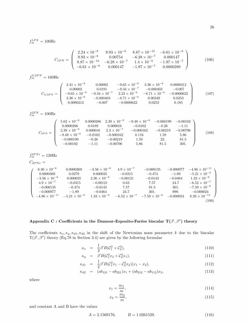
26

f1PNm = 100Hz

C1PN =

2.24 × 10−8 9.93 × 10−6 8.87 × 10−10 −6.61× 10−8

9.93 × 10−6 0.00754 −6.28× 10−7 0.0001478.87 × 10−10 −6.28 × 10−7 1.4 × 10−9 −1.97× 10−7

−6.61 × 10−8 0.000147 −1.97× 10−7 0.0000289

(106)

f3/2PNm = 160Hz

C3/2PN =

3.41 × 10−8 0.00002 −9.65 × 10−9 3.36 × 10−6 0.00002120.00002 0.0191 −9.34 × 10−7

−0.000403 −0.007−9.65 × 10−9

−9.34 × 10−7 2.23 × 10−8−8.71 × 10−6

−0.00006223.36 × 10−6

−0.000403 −8.71 × 10−6 0.00349 0.02530.0000212 −0.007 −0.0000622 0.0253 0.185

(107)

f2PNm = 100Hz

C2PN =

5.62 × 10−8 0.0000286 2.39 × 10−9−9.48 × 10−6

−0.000199 −0.001020.0000286 0.0189 0.000016 −0.0162 −0.26 −1.11

2.39 × 10−9 0.000016 2.3 × 10−7−0.000162 −0.00219 −0.00796

−9.48 × 10−6−0.0162 −0.000162 0.116 1.59 5.86

−0.000199 −0.26 −0.00219 1.59 22. 81.5−0.00102 −1.11 −0.00796 5.86 81.5 305.

(108)

f2PNem = 120Hz

C2PNe =

6.36 × 10−8 0.0000369 −3.56 × 10−8 4.9 × 10−7−0.000135 −0.000977 −4.86 × 10−11

0.0000369 0.0279 0.000035 −0.0315 −0.474 −1.89 −5.21 × 10−9

−3.56 × 10−8 0.000035 2.36 × 10−6−0.00121 −0.0143 −0.0464 1.33 × 10−9

4.9 × 10−7−0.0315 −0.00121 0.63 7.57 24.7 −6.52 × 10−7

−0.000135 −0.474 −0.0143 7.57 91.5 301. −7.59 × 10−6

−0.000977 −1.89 −0.0464 24.7 301. 999. −0.000024−4.86 × 10−11

−5.21 × 10−9 1.33 × 10−9−6.52 × 10−7

−7.59 × 10−6−0.000024 8.28 × 10−13

(109)

Appendix C : Coefficients in the Damour-Esposito-Farese biscalar T(β′, β′′) theory

The coefficients κo, κq, κd1, κd2 in the shift of the Newtonian mass parameter k due to the biscalarT(β′, β′′) theory (Eq.78 in Section 3.4) are given by the following formulae

κo =1

2β′B(C2

1 + C22), (110)

κq = β′B(C21x2 + C2

2x1), (111)

κd1 =1

2β′B(C2

1x1 − C22x2)(x1 − x2), (112)

κd2 = (ab121 − ab221)x1 + (ab212 − ab112)x2, (113)

where

x1 =m1

m, (114)

x2 =m2

m, (115)

and constant A and B have the values

A = 2.1569176, B = 1.0261529. (116)

27

C1 and C2 are sensitivities of the two bodies to changes of the scalar field. The functions ab are given by

ab121 = β′(−C2 − BC21 + (A − 3B)C2

2 − (A − B)2C2C21 + (117)

(2A2 − 7AB + 5B2)C22C2

1) + β′2B2(−3C31 + 2C2

1C22 + C4

1 +1

2C2C4

1 + AC22C4

1) +1

2β′′BC2

2 ,

ab212 = β′(−C1 − BC22 + (A − 3B)C2

1 − (A − B)2C1C22 + (118)

(2A2 − 7AB + 5B2)C21C2

2) + β′2B2(−3C31 + 2C2

1C22 + C4

1 +1

2C1C4

2 + AC21C4

2) +1

2β′′BC2

1 ,

ab221 = β′(−C2 −1

2B(C2

1 + C22) + (A − 3B)C2

2 − (A − B)C2(C21 + C2

2)+, (119)

1

2(2A2 − 7AB + 5B2)C2

2(C21 + C2

2)) + β′2B2(−3C32 + C2

2(C21 + C2

2)+,

C42 +

1

2C32C2

1 + AC21C4

2) +1

2β′′BC2

2 ,

ab112 = β′(−C2 −1

2B(C2

1 + C22) + (A − 3B)C2

1 − (A − B)C1(C21 + C2

2)+, (120)

1

2(2A2 − 7AB + 5B2)C2

1(C21 + C2

2)) + β′2B2(−3C31 + C2

1(C21 + C2

2)+,

C41 +

1

2C22C3

1 + AC22C4

1) +1

2β′′BC2

1 .

For a detailed exposition of the theory the reader should consult Ref.[37].

Appendix D: Detection of the known signal with a non-optimal filter

Suppose that we would like to know whether or not in a given data set x there is present a signal h. Weassume that the noise n in the data is additive. There are two alternatives:

NO SIGNAL : x = n

SIGNAL : x = h + n (121)

A standard method to determine which of the two alternatives holds is to perform the Neyman-Pearsontest[28]. This test consists in comparing the likelihood ratio Λ, the ratio of probability density distributionsof the data x when the signal is present and when the signal is absent, with a threshold. The thresholdis determined by the false alarm probability that we can tolerate (the false alarm probability is theprobability of saying that the signal is present when there is no signal). The test is optimal in thesense that it maximizes the probability of detection of the signal. In the case of Gaussian noise anddeterministic signal h the logarithm of Λ is given by

ln Λ = (x|h) − 1

2(h|h). (122)

Thus in this case the optimal test consists of correlating the data with the expected signal and it isequivalent to comparing the correlation G := (x|h) with a threshold. The probability distributions p0

and p1 of G when respectively the signal is absent and present are given by

p0(G; d) =1√

2πd2exp

[

−G2

d2

]

, (123)

p1(G; d) =1√

2πd2exp

[

− (G − d2)2

d2

]

, (124)

where d is the optimal signal-to-noise ratio d2 = (h|h) and we assumed that the noise is a zero meanGaussian process.

Let T be a given threshold. This means that we say that the signal is present in a given data set if G > T .The probabilities PF and PD of false alarm and detection respectively are given by

PF (T, d) =

∫ ∞

T

p0(G; d) dG, (125)

PD(T, d) =

∫ ∞

T

p1(G; d) dG (126)

28

In the Gaussian case they can be expressed in terms of the error functions.

PF (dT , d) =1

2erfc(

d2T√2d

), (127)

PD(dT , d) =1

2(1 + erf(

d2 − d2T√

2d), (128)

where erf and erfc are error and complementary error functions respectively [47]. and we have introducedfor convenience the quantity dT :=

√T that we call the threshold signal-to-noise ratio. In practice we

adopt a certain value of the false alarm probability that we can accept and from formula (127) we calculatethe detection threshold T.

Let F be a linear filter and let n be the additive noise in data x then

(x|F ) = (s|F ) + (n|F ). (129)

The signal-to-noise (S/N) ratio is defined by

(S/N)2 :=E1[(s|F )2]

E1[(n|F )2]=

(s|F )2

(F |F ). (130)

where E1 means expectation value when the signal is present. By Schwartz inequality we immediatelysee that (S/N) is maximal and equal to d when the linear filter is matched to the signal i.e. F = h. Thisis another interpretation of the matched filter - it maximizes the signal-to-noise ratio over all linear filters[28]. However when the noise is not Gaussian the matched filter is not the optimal filter; it does notmaximize probability of detection of the signal. We see that in the case of Gaussian noise the problem ofdetecting a known signal by optimal filter is determined by one parameter - the optimal signal-to-noiseratio d.

Suppose that because of certain restrictions of practical nature we cannot afford to use the optimal filterh and we use a suboptimal one - hN which is not perfectly matched to the signal. Thus (h|hN ) < (h|h).We denote

√

(h|hN ) by do and we assume that (hN |hN ) = (h|h) = d2. Our suboptimal correlationfunction is given by GN = (x|hN ) and its probability distributions pN0 and pN1 when respectively thesignal is absent and present are given by

pN0(GN ; d) =1√

2πd2exp

[

−G2N

d2

]

, (131)

pN1(GN ; d, do) =1√

2πd2exp

[

− (GN − d2o)

2

d2

]

. (132)

We see that the suboptimal detection problem is determined by two parameters - d and do, square rootsof the expectation values of the optimal and suboptimal correlations when the signal is present. The falsealarm and detection probabilities as in the optimal case can be expressed in terms of the error functions.

PF (dT , d) =1

2erfc(

d2T√2d

), (133)

PD(dT , d, do) =1

2(1 + erf(

d2o − d2

T√2d

). (134)

We see that the probability of false alarm for the suboptimal case is the same as in the optimal casehowever the probability of detection in the suboptimal case is always less then the probability of detectionin the optimal case since do < d and the error function erf(x) is an increasing function of the argumentx. The signal-to-noise ratio in the case of suboptimal linear filter hN is given by

(S/N)2 =(h|hN )2

(hN |hN )= d2(

do

d)4. (135)

Let us denote the ratio do/d by l. The ratio l measures the drop in the expectation value of the correlationfunction as a result of non-optimal filtering. We see that due to suboptimal filtering the signal-to-noise

29

ratio decreases by square of the factor l. We denote l2 by FF and following Ref.[14] call it the fittingfactor.

In our considerations we need to calculate the number of events that will be detected by linear filtering.We shall make a number of simplifying assumptions. We shall assume a Euclidean universe where in thesphere of radius ro we have one source and that at the distance ro the optimal signal-to-noise ratio is d.Moreover we shall assume that the magnitudes of the signal h and the suboptimal filter hN are inverselyproportional to the distance r from the source. Then the square roots dr and dor of the expectationvalues of the optimal and suboptimal correlations at the distance r are given by

dr =ro

rd, (136)

dor =ro

rdo. (137)

We assume that the sources are uniformly distributed in space. Then the expected number of detectedreal events N and NN in the optimal and the suboptimal case respectively is given by

N(dT , d) =4π

∫ ∞

0r2PD(dT , dr) dr

4π3

r3o

=

3

∫ ∞

0

x2PD(dT , d/x) dx (138)

NN(dT , d, do) =4π

∫ ∞

ror2PND(dT , d, do/r) dr

4π3

r3o

=

3

∫ ∞

0

x2PND(dT , d, do/x) dr. (139)

The assumptions that led to the above formulae mean that we neglect general relativistic, cosmologicaland evolutionary effects. Because of the noise even if there is no signal there is always a non zeroprobability that the correlation function crosses the threshold. Thus there will be a certain number NF

of false events. For a given optimal signal-to-noise ratio and a threshold dT this number is the same forboth the optimal and suboptimal filter and it is given by

NF =4π

∫ ∞

ro

r2PF (dT , d/r) dr4π3

r3o

= (140)

3

∫ ∞

o

x2PF (dT , d/x) dx.

We observe that in the Gaussian case the integrals in the formulae (138), (139), and (141) are convergenteven though we integrate over the all infinite Euclidean volume.

Appendix E: An approximate formula for the correlation function.

In this Appendix we shall derive an approximate formula for the correlation integral. Let us considerthe expression for the correlation function given by (36). The integrand of the correlation integral is theproduct of the integrand of the signal-to-noise integral Ind(f) considered in Section 2 and oscillatingfactor. We know that the Ind(f) is a fairly sharply peaked around a certain frequency f ′

o consequentlyto obtain a reasonable approximation we expand the phase around the frequency f ′

o. Keeping only theterms to the second order we get

Φ(f) ≃ 2π(f − f ′

o)∆t′ − ∆φ′′+, (141)

5

96

(f/f ′o − 1)2

(πf ′o)

5/3∆kTB + + O[(f/f ′

o − 1)3].

whereφ′′

o = φo − 2πf ′

ot′

o (142)

30

and

kE = k − 157

24

ke

(πf ′o)

19/9+ k1(πf ′

o)2/3 − k3/2(πf ′

o) + k2(πf ′

o)4/3 − 5

192

kD

(πf ′o)

2/3. (143)

We shall call kE an effective mass parameter. ∆kE is the difference in the effective mass parameter of thesignal and the filter. Thus in the above approximation the post-Newtonian signal can be parametrizedby one effective mass parameter kE . In other words the dimension of the parameter space of the filtersis effectively reduced. This last interpretation has been emphasized in [44] where 1st post-Newtoniancorrections to the phase were considered. The mass parameter estimated by Newtonian filter consideredin Section 3 is just the effective mass parameter. We stress that the parameter kE depends not only onthe parameters of the two-body system but also on the characteristic frequency f ′

o of the noise in thedetector.

The next step is to obtain a manageable approximation to the function Ind(f). We approximate it bya Gaussian function with the mean equal to the frequency f ′

o and the standard deviation equal to theHWHM σ′

o of the function Ind(f). We extend the range of integration from −∞ to +∞. We introducea normalization factor such that the integral of the approximate integrand is equal to the optimal signal-to-noise ratio d. It is then useful to introduce a reduced correlation integral H ′ = H/d2 where d is theS/N ratio. Thus our approximate formula for the reduced correlation integral takes the form

H ′

a =1√

2πσ2

∫ +∞

−∞

exp[−(f − f ′

o)/(2σ′

o2)] cos[2π(f − f ′

o)∆t′ + ∆φ′′ +5

96

(f/f ′o − 1)2

(πf ′o)

5/3∆kTB ] (144)

The above integral can be done analytically. It is convenient to introduce the following new variablesand new parameters

y =f − f ′

o√

2σ′o2

, (145)

ϑ′′ = ∆φ′′, (146)

τ = 2π∆t′√

2σ′o2, (147)

κ =5

96

∆kE

f ′o2(πf ′

o)5/3

2σ′

o2

(148)

then our integral takes a simple form

H ′

a(ϑ, τ, κ) =1√π

∫ +∞

−∞

exp[−y2] cos[−ϑ′′ + τy + κy2]dy. (149)

We see that in the new variables introduced above the reduced correlation integral is independent of thecharacteristics of the integrand Ind(f) i.e. f ′

o and σ′o. The analytic formula for the function H ′

a(ϑ′′, τ, κ)is given by

H ′

a(ϑ′′, τ, κ) =1

(1 + κ2)1/4exp[− τ2

4(1 + κ2)] cos[1/2(arctanκ − κτ2

2(1 + κ2)) − ϑ′′] (150)

By appropriate transformations given in Section 2 we can obtain approximate formulae to the corre-lation integral for an arbitrary choice of the time and the phase parameters. Let us first consider thetransformation given by Eq.(53). In the coordinates introduced above it takes the form

ϑ′′ = ϑ − 1√2τρ (151)

Then the approximate formula for the correlation function is given by

H ′

a(ϑ, τ, κ) =1

(1 + κ2)1/4exp[− τ2

4(1 + κ2)] cos[1/2(arctanκ − κτ2

2(1 + κ2)) +

1√2τρ − ϑ] (152)

We see that in these new coordinates for κ = 0 the correlation function oscillates with the maxima at thediscrete values of τ coordinate given by

τmax =2√

2π

ρn, (153)

31

where

ρ = f ′

o/σo (154)

and n is an integer. In the original coordinates Eq.(153) takes the form ∆t = 1/f ′o. Thus the correlation

integral oscillates with the period determined by the characteristic frequency of the noise of the detectorf ′

o.

The expressions for the correlation function for different choice of the time and the phase parameters canbe obtained by the following transformations. These are transformations given by Eqs.(39) and expressedin our dimensionless coordinates.

ϑ = ϑ′ +3

5κ′ρ2(1 − δ5/3), (155)

τ = τ ′ +3

4√

2κ′ρ′(1 − δ8/3) (156)

where

δ = f ′

o/fa. (157)

From the approximate formula for the correlation function obtained above we see that the correlationis given by the product of an oscillating cosine function and an envelope. In the cosine function thereare oscillations with the period of 1/f ′

o. The envelope function is exponentially damped if we move awayfrom the maximum at the center except for the direction given by τ = 0 along which the damping isleast. The equation of the ridge τ = 0 in the primed coordinates is given by

τ ′ = − 3

4√

2κ′ρ′(1 − δ8/3), (158)

and in the original coordinates it takes the form

∆t =5

256

1

(πf ′o)

8/3(1 − (

fa

f ′o

)8/3)∆kE . (159)

Consequently we conclude that the general appearance of the correlation function in coordinates ∆t′ and∆k is a series of peaks aligned along a straight line given by Eq.(159) above and occurring with theperiod 1/f ′

o in the time coordinate. Numerical investigation shows that the correlation integral exhibitsthese properties and that our analytic formula reproduces qualitatively its behaviour. The approximateformula obtained above may be a useful tool for developing algorithms to recognize the chirp signal in anoisy data set.

32

References

[1] K.S. Thorne, in 300 Years of Gravitation, edited by S.W. Hawking and W. Israel (Cambridge Uni-versity Press, Cambridge, 1987), pp. 330-458.

[2] R. Narayan, T. Piran, and A. Shemi, Astrophys. J. 379, L17 (1991).

[3] E. S. Phinney, Astrophys. J. 380, L17 (1991).

[4] A. V. Tutukov and L. R. Yungelson, Mon. Not. R. Astron. Soc. 260, 675 (1993).

[5] P.C. Peters, Phys. Rev. 136, B1224 (1964).

[6] L.S. Finn and D.F. Chernoff, Phys. Rev. D 47, 2198 (1993).

[7] A. Krolak, J.A. Lobo, and B.J. Meers, Phys. Rev. D 48, 3451 (1993).

[8] B. S. Sathyaprakash and S. V. Dhurandhar, Phys. Rev. D 44, 3819 (1993); ibid 49, 1707 (1994).

[9] K. D. Kokkotas, A. Krolak, and G. Tsegas, Class. Quantum Grav. 11, 1901 (1994).

[10] C. Cutler and E. Flanagan, Phys. Rev. D 49, 2658 (1994).

[11] C. Cutler, T. A. Apostolatos, L. Bildsten, L. S. Finn, E. E. Flanagan, D. Kennefick, D. M. Markovic,A. Ori, E. Poisson, G. J. Sussman and K. S. Thorne, Phys. Rev. Lett. 70, 2984 (1993).

[12] A. Krolak, in Gravitational Wave Data Analysis, edited by B.F. Schutz (Kluwer, Dordrecht, 1989),pp. 59-69.

[13] L. Blanchet, T. Damour, B. R. Iyer, C. M. Will and A. G. Wiseman, Gravitational-RadiationDamping of Compact Binary Systems to Second Post-Newtonian Order, submitted to Phys. Rev.Lett.(1995).

[14] T. A. Apostolatos, Ph. D. Thesis, California Institute of Technology (1994), unpublished.

[15] C. W. Lincoln and C. M. Will, Phys. Rev. D 42, 1123 (1990).

[16] L. Blanchet and B. S. Sathyaprakash, Phys. Rev. Lett. 74, 1067 (1995).

[17] R. V. Wagoner and C. M. Will, Astrophys. J. 210, 764 (1976);ibid 215, 984 (1977).

[18] E. Poisson, Phys. Rec.D 47, 1497 (1993).

[19] L. Blanchet and T. Damour, Phys. Rev. D46, 4301 (1992).

[20] A. G. Wiseman, Phys. Rev. D 48, 4757 (1993).

[21] L. Blanchet and G. Schafer, Class. Quantum Grav.10, 2699 (1993).

[22] L. E. Kidder, C. M. Will, and A. G. Wiseman, Phys. Rev.D 47, R4183 (1993).

[23] T. A. Apostolatos, C. Cutler, G. J. Sussman, and K. S. Thorne, Phys. Rev.D 49, 6274 (1994).

[24] S. Dhurandhar, A. Krolak, B. F. Schutz, and J. Watkins, Filtering the Gravitational Wave Signal ofa Coalescing Binary, (unpublished).

[25] L. Smarr, in Sources of Gravitational Radiation, edited by L. Smarr (Cambridge University Press,Cambridge, 1979).

[26] C. W. Helstrom, Statistical Theory of Signal Detection, 2nd ed. (Pergamon Press, London, 1968).

[27] S. V. Dhurandhar and B. F. Schutz, Phys. Rev. D 50, 2390 (1994).

[28] M. H. A. Davies, in Gravitational Wave Data Analysis, edited by B. F. Schutz (Kluwer, Dordrecht,1989), pp. 73-94.

[29] E. L. Lehmann, Theory of point estimation, (John Wiley & Sons, New York, 1983).

33

[30] P. Jaranowski, K. D. Kokkotas, A. Krolak, and G. Tsegas in preparation.

[31] A. Krolak and J. A. Lobo in preparation.

[32] N. Wex and G. Schafer, Class. Quantum Grav. 10, 2729 (1993).

[33] L.E. Kidder, C.M. Will, and A.G. Wiseman, Class. Quantum Grav. 9, L125 (1992); and Phys. Rev.D 47, 3281 (1993).

[34] C. M. Will and H. W. Zaglauer, Astrophys. J. 346, 366 (1989).

[35] C. M. Will, Theory and Experiment in Gravitational Physics, revised ed. (Cambridge UniversityPress, Cambridge, England, 1993).

[36] When this work was completed we learnt that accuracy of determination of the ω parameter in JFBDtheory by gravitational-wave observations from coalescing binaries has already been considered indetail by Clifford Will (C. M. Will, Phys. Rev. D 50,6058 (1994)) and a conclusion similar to ours wasreached. Moreover detection of scalar-type gravitational wave emission from gravitational collapsein JFKB theory by laser interferometers was investigated in paper: M. Shibata, K. Nakao, and T.Nakamura, Phys. Rev. D50, 7304 (1994).

[37] T. Damour and G. Esposito-Farese, Class. Quantum Grav.9, 2093 (1992).

[38] N. Wex, report (unpublished).

[39] A. Krolak in Proceedings of the Cornelius Lanczos International Centenar Conference, edited by J.D. Brown, M. T. Chu, D. C. Ellison and R. J. Plemmons (SIAM, Philadelphia, 1994) p. 482.

[40] K. D. Kokkotas, A. Krolak and G. Schafer in Proceedings of the XIVth Moriond Workshop ”ParticleAstrophysics, Atomic Physics and Gravitation, edited by J. Tran Thanh Van (Editions Frontieres,Gif-sur-Yvette, France, 1994).

[41] E. Flanagan, private communication.

[42] S. L. Finn, private communication.

[43] R. Balasubramanian and S. V. Dhurandhar, Phys. Rev. D 50, 6080 (1994).

[44] B. S. Sathyaprakash, Phys. Rev. D50, R7111 (1994).

[45] S. L. Finn, Phys. Rev. Lett. 73, 1878 (1994).

[46] P. C. Peters and J. Mathews, Phys. Rev. D 131, 435 (1963).

[47] The error function erf(x) is defined by

erf(x) =2√π

∫ x

0

exp(−t2) dt (160)

and the complementary error function erfc(x) is defined by

erfc(x) = 1 − erf(x). (161)