Estimation of Mediterranean crops evapotranspiration by means of remote-sensing based models

HESSD6, 1–38, 2009

Estimation ofMediterranean cropsevapotranspiration

M. Minacapilli et al.

Title Page

Abstract Introduction

Conclusions References

Tables Figures

J I

J I

Back Close

Full Screen / Esc

Printer-friendly Version

Interactive Discussion

Hydrol. Earth Syst. Sci. Discuss., 6, 1–38, 2009www.hydrol-earth-syst-sci-discuss.net/6/1/2009/© Author(s) 2009. This work is distributed underthe Creative Commons Attribution 3.0 License.

Hydrology andEarth System

SciencesDiscussions

Papers published in Hydrology and Earth System Sciences Discussions are underopen-access review for the journal Hydrology and Earth System Sciences

Estimation of Mediterranean cropsevapotranspiration by means ofremote-sensing based models

M. Minacapilli1, C. Agnese1, F. Blanda1, C. Cammalleri2, G. Ciraolo2, G. D’Urso3,M. Iovino1, D. Pumo1, G. Provenzano1, and G. Rallo1

1Dipartimento di Ingegneria e Tecnologie Agro-Forestali (ITAF), Universita di Palermo, Italy2Dept. of Hydraulic Engineering and Environmental Applications, Universita di Palermo, Italy3Dept. Agricultural Engineering and Agronomy, University of Naples “Federico II”, Italy

Received: 24 October 2008 – Accepted: 5 November 2008 – Published: 5 January 2009

Correspondence to: M. Minacapilli ([email protected])

Published by Copernicus Publications on behalf of the European Geosciences Union.

1

http://www.hydrol-earth-syst-sci-discuss.net

http://www.hydrol-earth-syst-sci-discuss.net/6/1/2009/hessd-6-1-2009-print.pdf

http://www.hydrol-earth-syst-sci-discuss.net/6/1/2009/hessd-6-1-2009-discussion.html

http://creativecommons.org/licenses/by/3.0/

HESSD6, 1–38, 2009



Title Page



Tables Figures

J I

J I

Back Close

Full Screen / Esc



Abstract

Actual evapotranspiration from typical Mediterranean crops has been assessed in aSicilian study area by using Surface Energy Balance and Agro-Hydrological models.Both modelling approaches require remotely sensed data to estimate evapotranspi-ration fluxes in a spatially distributed way. The first approach exploits visible (VIS),5

near-infrared (NIR) and thermal (TIR) observations to solve the surface energy bal-ance equation. To this end two different schemes have been tested: the two-sourcesTSEB model, where soil and vegetation components of the surface energy balanceare treated separately, and the widely used one-source SEBAL model, where soil andvegetation are considered as a sole source. Actual evapotranspiration estimates by10

means of the two surface energy balance models have been compared with the resultsof the Agro-Hydrological model SWAP, applied in a spatially distributed way to simu-late one-dimensional water flow in the soil-plant-atmosphere continuum. In this lattermodel, remote sensing data in the VIS and NIR spectral ranges have been used toinfer spatially distributed vegetation parameters needed to set up the upper boundary15

condition of SWAP. In the comparison presented here, actual evapotranspiration val-ues obtained from the application of the soil water balance model SWAP have beenconsidered as the reference.

Considering that the study area is characterized by typical Mediterranean sparsevegetation, i.e. olive, citrus and vineyards, we focused the attention on the main con-20

ceptual differences between SEBAL and TSEB. Airborne hyperspectral data acquiredduring a NERC campaign in 2005 have been used. The results of the investigation evi-denced that the remote sensing two-sources approach used in TSEB model describesturbulent and radiative surface fluxes in a more realistic way than the one-source ap-proach.25

2





HESSD6, 1–38, 2009



Title Page



Tables Figures

J I

J I

Back Close

Full Screen / Esc



1 Introduction

The estimation of temporal and spatial distribution of actual evapotranspiration (ET) isan essential step for mapping crop water requirements and for water management pur-poses, especially in Mediterranean areas where water scarcity and semiarid climatecause often fragility and severe damage in the agro-ecosystems. The determination5

of ET in water-limited conditions is not an easy task, due to the heterogeneity andcomplexity of involved hydrological and biophysical processes. During recent years,several procedures and models have been developed to simulate mass and energy ex-change in the Soil-Plant-Atmosphere (SPA) system (Feddes et al., 1978; Bastiaanssenet al., 2007). In particular, deterministic models have been proposed for detailed simu-10

lation of all the components of the water balance, including crop growth, irrigation andsolute transport (Vanclooster et al., 1994; van Dam et al., 1997; Droogers et al., 2000;Ragab, 2002). These models have been developed for site-specific applications butthey have seldom been applied to large areas, due to the complexity in the acqui-sition of input data, often characterised by spatial and temporal variability. To over-15

come this problem, techniques have been suggested which involve the use of GIS (Liuet al., 2007a, b; Liu, 2009) and Remote Sensing techniques to gather quantitative in-formation on the temporal and spatial distribution of various vegetation parameters, i.e.albedo, crop coefficient, leaf area index (Choudhury et al., 1994; D’Urso et al., 1999;Schultz and Engman, 2000). These studies are based on the fact that crop canopy re-20

flects solar radiation, which can be measured with a radiometer at various wavelengthin the visible and near-infrared (VIS/NIR) spectral range. The feasibility of using re-motely sensed crop parameters in combination of Agro-Hydrological models has beeninvestigated in several studies (D’Urso, 2001; D’Urso and Minacapilli, 2006; Immerzeelet al., 2008; Crown et al., 2008; Minacapilli et al., 2008) with the aim of enabling the25

spatially distributed evaluation of water balance components in the SPA system.A further contribution offered by Remote Sensing techniques has been the devel-

opment of operational methods for the direct estimation of actual evapotranspiration

3





HESSD6, 1–38, 2009



Title Page



Tables Figures

J I

J I

Back Close

Full Screen / Esc



based on the Surface Energy Balance (SEB) approach, which exploits thermal infrared(TIR) observations of the Earth’s surface acquired from satellite and/or airborne plat-forms (Norman et al., 1995; Chehbouni et al., 1997; Bastiaanssen et al., 1998a, b; Su,2002). In the recent years, several SEB schemes have been developed (Schmuggeet al., 2002) with varying degree of complexity. In all these schemes the evapotran-5

spiration is derived in terms of latent heat flux, λET (W m−2), ad it is computed as theresidual of the surface energy balance equation:

λET = Rn − G0 − H (1)

where Rn (W m−2) is the total net radiation, G0 (W m−2) is the soil heat flux, and H(W m−2) is the sensible heat flux.10

The largest uncertainty in estimating λET is due to the computation of H . Followingthe bulk resistance or “one-source” approach for a natural surface, the basic equationfor soil-plus-canopy sensible heat flux, H , is given by:

H =ρcp(T0h − Ta)Ra + Rex

=ρcp(T0h − Ta)

Rah(2)

where ρ (kg m−3) is the air density, cp is the specific heat of air (J kg−1 K−1), T0h (K)15

is the so-called “aerodynamic surface temperature” (Kalma and Jupp, 1990), definedas the air temperature “which satisfies the bulk resistance formulation for sensible heattransport, H” (Kustas et al., 2007), Ta (K) is the air temperature at some referenceheight, Ra (s m−1) is the aerodynamic resistance (Brutsaert, 1982), Rex (s m−1) is theexcess resistance associated with heat transport and Rah (s m−1) is the total resistance20

to heat transport across the temperature difference (T0h–Ta). Since the aerodynamicsurface temperature is usually unknown, the common approach used in various single-source schemes is to empirically relate the radiative surface temperature, Tr , to T0h ordirectly to the term (T0h–Ta).

Differently, the so-called “two-sources” approach (Shuttleworth and Wallace, 1985;25

Shuttleworth and Gurney, 1990; Norman et al., 1995) considers the partitioning of4





HESSD6, 1–38, 2009



Title Page



Tables Figures

J I

J I

Back Close

Full Screen / Esc



fluxes in two components, i.e. soil and vegetation, as viewed from a remote sensorwith an incidence angle θ. Hence, the total sensible heat flux is given by the sum ofHs, related to soil, and Hc, related to the vegetation canopy:

H = Hs + Hc (3)

Hc = ρcp

[Tc − TaRah

](4)5

Hs = ρcp

[Ts − TaRs + Rah

](5)

In Eqs. (4) and (5) Tc and Ts (K) are, respectively, the canopy and soil aerodynamictemperatures and Rs (s m−1) is the soil resistance to the heat transfer (Goudriaan,1977; Norman et al., 1995; Kustas and Norman 1999a, b).

In this paper the SEBAL single-source model (Bastiaanssen et al., 1998a, b) and the10

TSEB two-sources model (Norman et al., 1995) have been applied to determine thesurface energy fluxes in an area located in the South West of Sicily and characterizedby typical Mediterranean crops.

Of particular interest to this study is the use of airborne high-resolution (3 m×3 m)remote sensing data in the VIS/NIR and TIR regions providing a detailed observation15

of spectral reflectance and surface temperature. The remote acquisition has beentaken during an intensive field campaign carried out in 2005, where intensive dataincluding soil and hydrological measurements have been collected. This intensive fielddata set has been used to implement the soil water balance model SWAP (van Damet al., 1997) in a spatially distributed way. The spatial distribution of canopy parameters20

has been derived from airborne observations in the visible and near-infrared ranges,and it has been used to define the upper boundary condition of the SWAP model(D’Urso et al., 1999). The output of the spatially distributed SWAP includes actualevapotranspiration calculated from the root water uptake, validated by means of soilwater content measurements. As such, these ET values have been considered as the25

“reference” in the comparison between SEBAL and TSEB energy balance models, in5





HESSD6, 1–38, 2009



Title Page



Tables Figures

J I

J I

Back Close

Full Screen / Esc



absence of a sufficiently dense network of flux instrumentations installed in the studyarea, which would have been impossible to install in an efficient way due to the highlevel of agricultural fragmentation.

2 Models description

SEBAL, TSEB and SWAP models use different approaches to calculate actual evap-5

otranspiration. Key differences and peculiarities of the models are described in thefollowing subsections.

2.1 SEBAL and TSEB models

A first application of the models in the same study area can be found in Ciraoloet al. (2006) and in Minacapilli et al. (2007). A detailed description of SEBAL and10

TSEB models can be found in Norman et al. (1995), Bastiaanssen et al. (1998a, b),Kustas and Norman (1999a, b). Here we only describe the main differences of themodels.

In both models, the estimation of total net radiation, Rn, can be obtained by com-puting the net available energy considering the rate lost by surface reflection in the15

shortwave (0.3/2.5 µm) and emitted in the longwave (6/100 µm):

Rn = (1 − α)Rswd + ε0

(ε′σT 4

a − σT 40

)(6)

where Rswd (W m−2) is the global incoming solar radiation, α (–) is the surface albedo,ε′ is the atmospheric emissivity (–), ε0 is the surface emissivity (–), σ (W m−2 K−4) is theStefan-Boltzmann constant, Ta (K) is the air temperature, and T0 (K) is the land surface20

temperature derivable from thermal remote sensing data. Moreover, the TSEB modelsplits the net radiation Rn between canopy (Rn,c) and soil (Rn,s), that is computed as

6





HESSD6, 1–38, 2009



Title Page



Tables Figures

J I

J I

Back Close

Full Screen / Esc



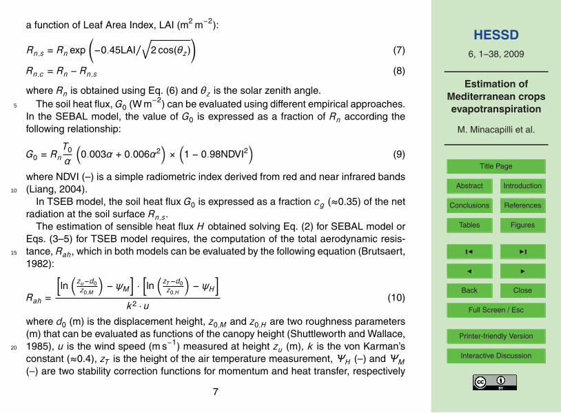
a function of Leaf Area Index, LAI (m2 m−2):

Rn,s = Rn exp(−0.45LAI/

√2 cos(θz)

)(7)

Rn,c = Rn − Rn,s (8)

where Rn is obtained using Eq. (6) and θz is the solar zenith angle.The soil heat flux, G0 (W m−2) can be evaluated using different empirical approaches.5

In the SEBAL model, the value of G0 is expressed as a fraction of Rn according thefollowing relationship:

G0 = RnT0

α

(0.003α + 0.006α2

)×(

1 − 0.98NDVI2)

(9)

where NDVI (–) is a simple radiometric index derived from red and near infrared bands(Liang, 2004).10

In TSEB model, the soil heat flux G0 is expressed as a fraction cg (≈0.35) of the netradiation at the soil surface Rn,s.

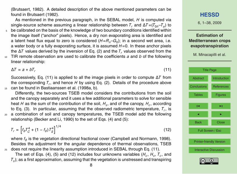
The estimation of sensible heat flux H obtained solving Eq. (2) for SEBAL model orEqs. (3–5) for TSEB model requires, the computation of the total aerodynamic resis-tance, Rah, which in both models can be evaluated by the following equation (Brutsaert,15

1982):

Rah =

[ln(zu−d0z0,M

)− ψM

]·[ln(zT−d0z0,H

)− ψH

]k2 · u

(10)

where d0 (m) is the displacement height, z0,M and z0,H are two roughness parameters(m) that can be evaluated as functions of the canopy height (Shuttleworth and Wallace,1985), u is the wind speed (m s−1) measured at height zu (m), k is the von Karman’s20

constant (≈0.4), zT is the height of the air temperature measurement, ΨH (–) and ΨM(–) are two stability correction functions for momentum and heat transfer, respectively

7





HESSD6, 1–38, 2009



Title Page



Tables Figures

J I

J I

Back Close

Full Screen / Esc



(Brutsaert, 1982). A detailed description of the above mentioned parameters can befound in Brutsaert (1982).

As mentioned in the previous paragraph, in the SEBAL model, H is computed viasingle-source scheme assuming a linear relationship between Tr and ∆T=(T0h–Ta) tobe calibrated on the basis of the knowledge of two boundary conditions identified within5

the image itself (“anchor” pixels). Hence, a dry non evaporating area is identified anda latent heat flux equal to zero is considered (H=Rn–G0); in a second wet area, i.e.a water body or a fully evaporating surface, it is assumed H=0. In these anchor pixelsthe ∆T values derived by the inversion of Eq. (2) and the Tr values observed from theTIR remote observation are used to calibrate the coefficients a and b of the following10

linear relationship:

∆T = a + bTr (11)

Successively, Eq. (11) is applied to all the image pixels in order to compute ∆T fromthe corresponding Tr , and hence H by using Eq. (2). Details of the procedure abovecan be found in Bastiaanssen et al. (1998a, b).15

Differently, the two-sources TSEB model considers the contributions from the soiland the canopy separately and it uses a few additional parameters to solve for sensibleheat H as the sum of the contribution of the soil, Hs, and of the canopy, Hc, accordingto Eq. (3). In particular, assuming that the observed radiometric temperature, Tr , isa combination of soil and canopy temperatures, the TSEB model add the following20

relationship (Becker and Li, 1990) to the set of Eqs. (4) and (5):

Tr =[fθT

4C + (1 − fθ) T 4

S

]1/4(12)

where fθ is the vegetation directional fractional cover (Campbell and Normann, 1998).Besides the adjustment for the angular dependence of thermal observations, TSEBdoes not require the linearity assumption introduced in SEBAL through Eq. (11).25

The set of Eqs. (4), (5) and (12) includes four unknowns variables (Hc, Hs, Tc, andTs); as a first approximation, assuming that the vegetation is unstressed and transpiring

8





HESSD6, 1–38, 2009



Title Page



Tables Figures

J I

J I

Back Close

Full Screen / Esc



at the potential rate, the TSEB model uses the Priestly-Taylor equation (Priestly andTaylor, 1972) to estimate the latent heat flux λETc as:

λETc = Rn,c − Hc = αp∆

∆ + γRn,c (13)

where αp (–) is the Priestly–Taylor parameter, which is initially set to 1.26 (“potential”condition) and progressively adjusted, as explained below. In Eq. (13) ∆ is the slope5

of the saturation vapour pressure-temperature curve at TC (Pa K−1) and γ is the psy-chrometric constant. Using Eq. (8) to compute Rn,c, Eq. (13) is solved for Hc and thenEq. (4) is inverted to estimate Tc as:

Tc =(

1 − α ∆∆ + γ

)Rn,c

rcρcp

+ Ta (14)

The constraint in Eq. (12) can then be inverted to estimate Ts as:10

Ts =

(T 4r − fθT

4c

1 − fθ

)1/4

(15)

Prediction of Ts allows for calculation of Hs via Eq. (5) using, for Rs, a relationshipsuggested by the Authors in the original paper of the model (Norman et al., 1995;Kustas and Norman 1999a, b). Consequently the soil evaporation Es can be computedas:15

Es = G0 − Hs = cgRn,s − Hs (16)

If the vegetation canopy is undergoing water stress, Eq. (13) will lead to an overes-timation of λETc, which turns in a negative value of Es in Eq. (16). This problem isaddressed by iteratively decreasing αp in Eq. (13) until a positive Es is reached (Kus-tas and Norman, 1999).20

9





HESSD6, 1–38, 2009



Title Page



Tables Figures

J I

J I

Back Close

Full Screen / Esc



For both the models, once the Rn, G0 and H spatial distributions are obtained, theλET (W m−2) spatial distribution is computed using Eq. (1). Finally, the daily evapo-transpiration ETd (mm d−1) can be obtained by the time integration of λET using theevaporative fraction parameter, Λ (Menenti and Choudhury, 1993):

Λ =λET

Rn − G0(17)5

Several studies (Brutsaert and Sugita, 1992; Crago, 1996) demonstrated that, withindaytime hours, the Λ(0−1) values are almost constant in time. This fact suggests touse the Λ parameter as a temporal integration parameter. Following this hypothesis,the daily evapotranspiration, ETd (mm d−1), can be derived using the equation:

ETd = ΛRn,24

λ(18)10

where λ (MJ kg−1) is the latent heat of vaporization and Rn,24 represents the averagednet daily radiation, that can be derived by direct measurement or by using the classicalformulation proposed in FAO 56 paper (Allen et al., 1998).

2.2 The agro-hydrological SWAP model

SWAP (Soil-Water-Atmosphere-Plant) is a one-dimensional physically based model15

for water, heat and solute transport in saturated and unsaturated soil, and includesmodules to simulate irrigation practice and crop growth (Kroes and van Dam, 2003).SWAP simulates the vertical soil water flow and solute transport in close interactionwith crop growth. Richards’ equation (Richards, 1931), including root water extraction,is applied to compute transient soil water flow:20

C(h)∂h∂t

=∂∂z

[K (h)

(∂h∂z

+ 1)]

+ S(h) (19)

under specified upper and lower boundary conditions. In Eq. (19) z (cm) is the verticalcoordinate, assumed positive upwards, t (d) is time, C (cm−1) is the differential moisture

10





HESSD6, 1–38, 2009



Title Page



Tables Figures

J I

J I

Back Close

Full Screen / Esc



capacity, K (h) (cm d−1) is the soil hydraulic conductivity function and S (d−1) is the rootuptake term that, in the case of uniform root distribution, is defined by the followingequations:

S(h) = αw (h)Tp|zr |

(20)

Tp = Kc × ET0[1 − exp(−KgrLAI)

](21)5

in which Tp (cm d−1) is the potential transpiration, zr (cm) is the rooting depth andαw (–) is a h-dependant reduction factor which accounts for water deficit and oxygenstress (Feddes et al., 1978), Kc (–) is the crop coefficient, ET0 (cm d−1) is the referenceevapotranspiration and Kgr (–) is an extinction coefficient for global solar radiation.The numerical solution of Eqs. (19), (20) and (21) is possible after specifying initial,10

and upper and lower boundary conditions and the soil hydraulic properties, i.e. thesoil water retention curve, θ(h), and the soil hydraulic conductivity function, K (h) areknown; detailed field and/or laboratory investigations are therefore needed.

In this study, the application of SWAP has been carried out in a spatially distributedway, according to the procedure suggested by D’Urso (2001). The study area has15

therefore been discretized in individual one-dimensional units, with homogenous soiland canopy parameters. Canopy parameters such crop coefficient, Kc, and the leafarea index, LAI, have been determined by using the remote sensing approach pro-posed by D’Urso et al. (1999, 2001). Thus, for a given set of climatic variables, usingthe above mentioned approach, the spatial distributions of the potential evapotran-20

spiration has been derived, and this information has been used to define – in eachelementary unit – the upper boundary condition of the soil water balance model SWAP,represented by Eq. (21). A detailed description of the entire procedure can be found inD’Urso (2001) and in Minacapilli et al. (2008).

11





HESSD6, 1–38, 2009



Title Page



Tables Figures

J I

J I

Back Close

Full Screen / Esc



3 Case study and data collection

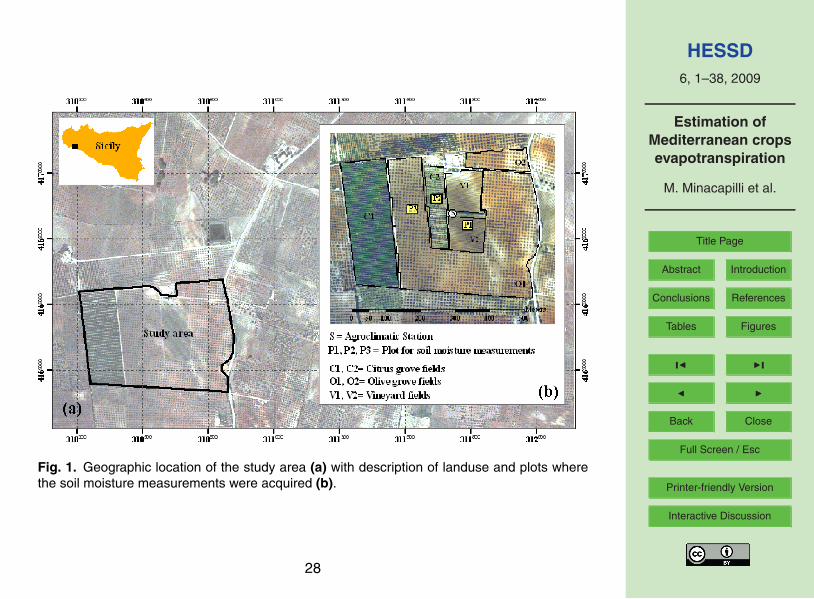
The study area covers an extension of approximately 20 ha, located in the south-western coast of Sicily (Fig. 1). Orchard crops (mainly olives, grapes and citrus) rep-resent the dominant vegetation; soil can be classified as silty clay loam (USDA classi-fication). During 2005, daily meteorological data (incoming short-wave solar radiation,5

air-temperature and humidity, wind speed and rainfall) have been acquired with stan-dard meteorological instrumentations. A soil survey has been carried out to identify themain soil hydraulic parameters, needed as input in SWAP. In particular temporal vari-ability of soil moisture contents in the different plots (Fig. 1) and at different depths weremeasured using TDR techniques and Diviner 2000 Sentek capacitive sensors. These10

values have been used for validating SWAP in selected locations. Canopy parametersand radiometric surface temperatures have been acquired during a airborne campaignsupported by NERC (National Environment Research Council, UK).

3.1 Aircraft remote sensing pre-processing

The NERC airborne campaign has taken place on 16 May 2005 at about noon (local15

time). The flight altitude of 1400 m and the optical characteristics of the ATM sensor(Airborne Thematic Mapper) has produced images with a nominal spatial resolution(pixel size) of 3×3 m. ATM has 8 spectral bands in the visible and near-infrared ranges(VIS/NIR) 2 in the short-wave infrared (SWIR) and 1 in the thermal infrared region(TIR). At the same time of the acquisition flight, a field survey was carried out by mea-20

suring spectral and vegetation parameters in correspondence of predefined homoge-neous targets. Spectral measurements on water, bare soil and grass surfaces havebeen acquired by using an ASDI FieldSpect HH spectroradiometer; these measure-ments have been used for the radiometric and atmospheric corrections of the VIS-NIRimages of ATM by using the empirical line method (Slater et al., 1996). The result-25

ing surface reflectance values have been successively used to calculate the surfacealbedo and the vegetation indexes. At-surface temperature measurements have been

12





HESSD6, 1–38, 2009



Title Page



Tables Figures

J I

J I

Back Close

Full Screen / Esc



made in selected locations simultaneously to the flight, in order to perform an empir-ical calibration of the thermal images acquired by the ATM sensor. Figure 2a and bshows the accuracy obtained from the abovementioned corrections in both VIS/NIRand TIR bands. The geometric correction of the entire data set has been performedusing the NERC Azgcorr software, that performs geocorrection of images using aircraft5

navigation data and Digital Elevation Model (DEM) of the acquired zone.

3.2 SWAP model parameterization

The minimum data-set required for the application of the SWAP model includes fourmain information types: i) soil hydraulic parameters; ii) lower boundary condition, de-fined by the groundwater table or the water flux to or from an existent aquifer; iii) pa-10

rameters related to the upper boundary, i.e. rainfall and/or potential evapotranspiration;iv) soil moisture content or soil water pressure head profile for the initial condition.

Maps of soil hydraulic properties have been realised by means of a soil survey withan intensive undisturbed sampling. Laboratory investigations on the undisturbed soilcores have been carried to determine the soil water hydraulic and retention curves15

required in input for SWAP. The saturated hydraulic conductivity, Ks (cm d−1) has beendetermined by means of the constant head technique (Reynolds et al., 2002); soil watercontent θ has been determined in correspondence of a set of pressure head values,h, ranging from −5 to −15 300 cm by means of a hanging water column apparatus(Burke et al., 1986) and a pressure plate apparatus (Dane and Hopmans, 2002). The20

water retention function of van Genuchten (1980) has been fitted to the measured θ-hvalues by using the RETC (RETention Curve) code (van Genuchten et al., 1991). Theunsaturated hydraulic conductivity function has been derived by using the Mualem-vanGenuchten model (van Genuchten, 1980). Due to the limited spatial variability of soilproperties, it has been possible to consider an unique soil profile for the simulations of25

soil water balance in the study area, which characteristics are summarised in Table 1.The intensive field measurements collected during 2005 showed that the soil water

content was always near to saturated value from 1.2 m to lower depths. Therefore, the13





HESSD6, 1–38, 2009



Title Page



Tables Figures

J I

J I

Back Close

Full Screen / Esc



simulations were carried out considering a zero flux at the bottom of the soil profile.The upper boundary condition, in terms of potential evapotranspiration ETp (mm d−1)

was obtained by multiplying the reference evapotranspiration (ET0) with the crop coef-ficients (Kc). The ET0 was determined by using the Penman-Monteith equation (Allenet al., 1998), while the spatial distribution of the crop coefficients was obtained using the5

remote sensing approach proposed by D’Urso (2001). As mentioned in Sect. 2.2, theprocedure requires the knowledge of canopy parameters such as the surface albedo,α, the leaf area index, LAI, the crop height hc, and the standard set of meteorologicaldata (wind speed at reference height, shortwave incoming solar radiation, air tempera-ture and humidity). For the study area, the crop parameters have been derived using10

spectral reflectance values acquired from the ATM VIS/NIR bands. In particular, thesurface albedo have been computed as weighted average over VIS and NIR spectrumassuming as weighting parameter the solar irradiance for each bandwith (Liang, 2004).The LAI spatial distribution has been detected using the following semi-empirical rela-tionship (Clevers, 1989):15

LAI = − 1α∗ ln

(1 − WDVI

WDVI∞

)(22)

in which WDVI is a vegetation index derived from ATM red and near-infrared bands(Clevers, 1989), WDVI∞ is the asymptotic value of WDVI for LAI→∞, and α∗ is anextinction coefficient, denoting the increase of LAI for a unit increase of WDVI, thathas to be estimated from simultaneous measurements of LAI and WDVI. In our case,20

the calibration of Eq. (22) was preliminarily carried out by in-situ LAI measurementscollected with the portable instrument LAI2000 (Li-Cor, Lincoln, NE). A complete de-scription of the leaf area index estimation conducted for the study area is given inMinacapilli et al. (2005, 2008). Otherwise, as suggested by other authors (Andersonet al., 2004) the crop heigh, hc, has been calculated using a polynomial relationship25

derived from field data of LAI and hc. Once derived α, LAI and hc crop parameters,the pixel based spatial distribution of crop coefficients Kc has been derived for the dateof the NERC airborne overflight (16 May 2005, J=135) with the resolution of 3 m×3 m

14





HESSD6, 1–38, 2009



Title Page



Tables Figures

J I

J I

Back Close

Full Screen / Esc



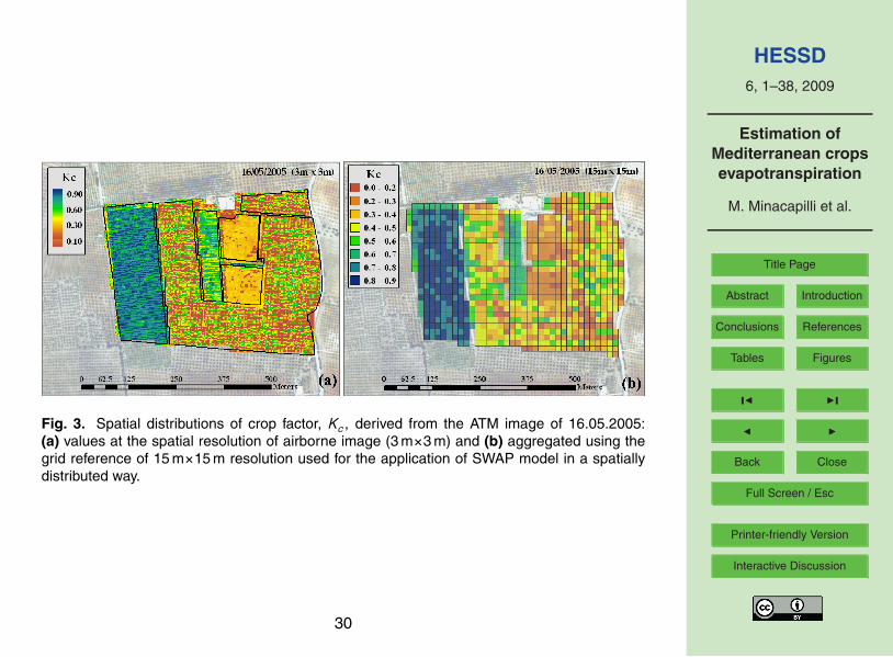
(Fig. 3a); afterwards the values were spatially aggregated using a regular vector gridhaving a mesh size of 15 m×15 m (Fig. 3b) and corresponding to the set of single unitsthat will be used for the spatially distributed application of SWAP model.

Considering that, with the exception of the grape, all the other crops in the studyarea are evergreen, the only ATM airborne surveys, acquired on 16.05.2005 has been5

sufficient to derive crop coefficients values as input in the SWAP simulation period(15.04.2005–15.05.2005). At the starting date, a lumped value of the crop coefficientfor grape was derived from specific literature (Allen et al., 1998) by assuming a linearvariation during the period of simulation.

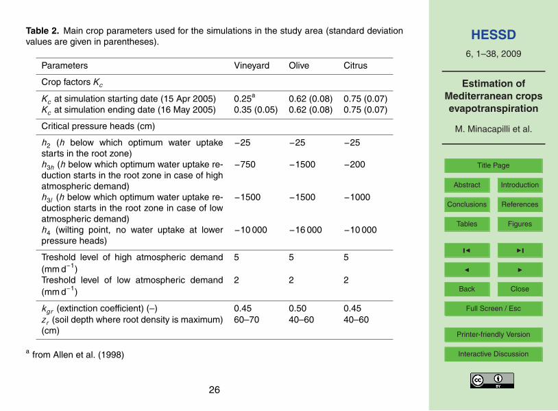
Others crop parameters required by SWAP, i.e. kgr , zr and the critical pressure head10

values defining the reduction factor αw in Eq. (20), were taken from specific literature(Taylor and Ashcroft, 1972; Doorenbos and Kassam, 1979; Wesseling et al., 1991) withsome minor adaptations based on local observations. Crop parameters for the casestudy used for the simulations are summarized in Table 2.

4 Results and discussion15

The following results focus on the crop evapotranspiration estimated using both en-ergy (SEBAL and TSEB) and soil-water (SWAP) balance modelling approaches. Inparagraph 4.1, a preliminary validation of SWAP model at field scale is discussed;afterwards the application of SWAP model has been replicated in a distributed wayusing the approach described in paragraph 3.2. Finally, in paragraph 4.2 evaluation of20

the spatially patterns of surface energy fluxes and evapotraspiration values predictedby SEBAL and TSEB models is showed, as well as the final comparison of spatiallydistributed crop evapotranspiration estimated with the three different approaches.

15





HESSD6, 1–38, 2009



Title Page



Tables Figures

J I

J I

Back Close

Full Screen / Esc



4.1 Validation of SWAP at field scale and its spatially distributed application

The validation of SWAP has been carried out in correspondence of three different loca-tions, inside the experimental farm (Fig. 1), where measurements of soil water contenthave been continuously acquired during the simulation period. Mean Kc values for thedifferent crop types at these locations – and extracted from the map in Fig. 3a – are5

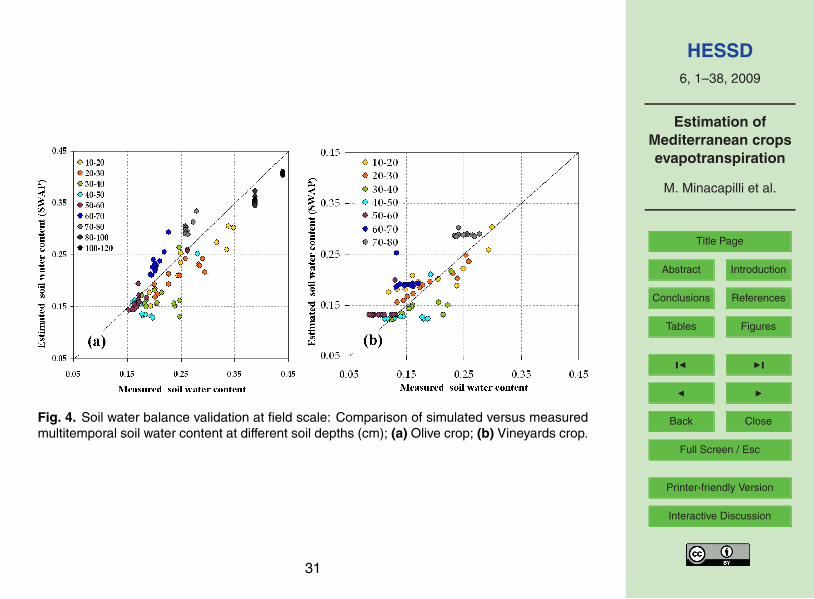
summarized in Table 2. As evidenced in the plots of Fig. 4, a good agreement has beenfound between measured and simulated soil water content; a more complete descrip-tion of the validation procedures of SWAP model at field scale can be found in Blanda(2007).

From the application of the SWAP model to the study area, we have simulated the10

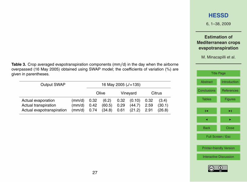
actual evapotranspiration for each elementary unit on a daily basis; an example of theresulting map for the simulation day corresponding to the NERC flight is shown in Fig. 5.A summary of the values obtained for each crop type is given in Table 3. From Fig. 5,we may notice a significant spatial variability in evapotranspiration in the olive orchard,as highlighted by the higher coefficient of variation (34.8%). This behaviour is driven15

largely by variations of the fraction of ground covered by canopy (fraction cover) insideeach 15 m×15 m simulated unit. Otherwise for the citrus grove the greater uniformity ofthe fraction cover involves a lower spatial variability in evapotranspiration patterns. Onthe same date the vineyards was less developed so that less evapotranspiration rateswas recognized.20

4.2 Estimating ET by SEB models and final comparison

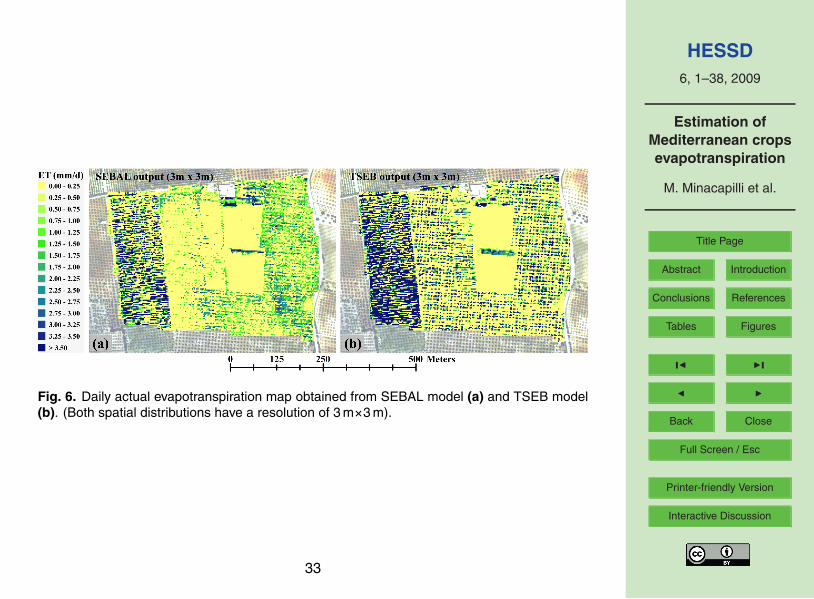
The two surface energy balance models, i.e. SEBAL and TSEB, have been applied byusing VIS/NIR and TIR data acquired during the NERC campaign on 16 May 2005 asdescribed in Sect. 3.1. The output of these models has been compared in terms ofspatial patterns of actual ET, as well as in terms of statistical correlation on a pixel-25

by-pixel basis. The resulting maps of ET, as displayed in Fig. 6a and b, have beenproduced with a spatial resolution of 3 m; thanks to this high spatial resolution of TIR

16





HESSD6, 1–38, 2009



Title Page



Tables Figures

J I

J I

Back Close

Full Screen / Esc



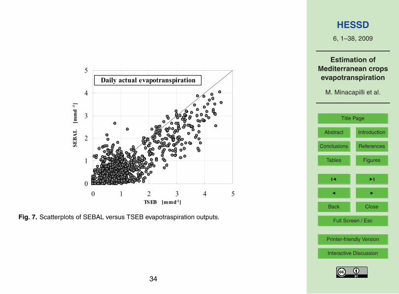
data, it is possible to observe in great detail the spatial patterns of ET, which may im-prove the interpretation of the model results. The plot in Fig. 7 is a pixel-wise scatterplotof the daily ET values obtained with the two models. This plot evidences that SEBALproduces an underestimation of ET compared to TSEB of about 1 mm d−1. This under-estimation can be explained by giving a closer look to the values of the different terms5

of the energy balance, as shown by Fig. 8, where maps and scatterplots of sensibleheat flux H and soil heat flux G are represented. From this figure, we may notice thatSEBAL gives a systematic strong overestimation of H , which is not compensated bythe opposite behaviour of G. This effect, which has been already observed in othersimilar studies (Savige et al., 2005; Ciraolo et al., 2006; Minacapilli et al., 2007), has10

been related to an underestimation of the total resistance to the heat transport oversparsely vegetated surface, since SEBAL does not take into account the soil–canopyinteractions. Diversely, TSEB model based on the partitioning between soil and canopyis able to provide a more physically-based picture of the surface resistances involved.As a result, being the available energy (Rn−G) quite similar between the two mod-15

els, the overestimation of sensible heat flux in SEBAL is mainly responsible for thedisagreement in λET shown in Fig. 7.

In the first phase, assuming the actual evapotranspiration values simulated by SWAPas reference, the ET values obtained using SEBAL and TSEB models have been spa-tially aggregated by using the same 15 m×15 m grid adopted in the SWAP simulation.20

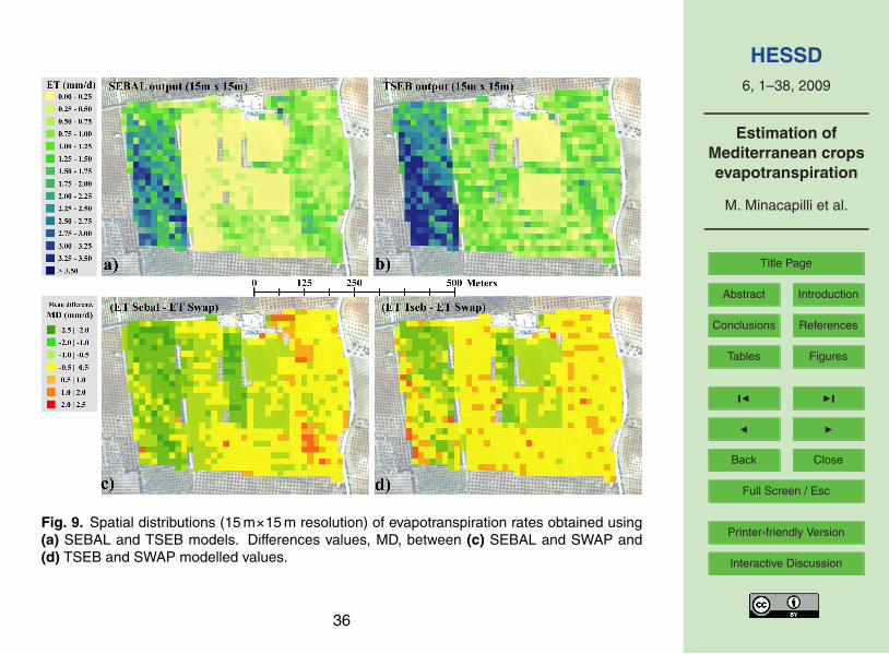
A further comparison has then been carried out by considering the spatial distribu-tion of the different values of ET, as shown by Fig. 9a and b. Again, we notice thatthe different scale does not compensate for the difference in ET between TSEB andSEBAL, already observed at 3 m×3 m pixel resolution.

Finally, an assessment of models performances were evaluated computing the dif-25

ference MD (mm/d) between the actual ET obtained by means of SEBAL/TSEB andSWAP.

Maps presenting the spatial distribution of MD values are shown in Fig. 9c and d: forboth models MD values range from −2.5 to 2.5 mm/d with a smaller mean value using

17





HESSD6, 1–38, 2009



Title Page



Tables Figures

J I

J I

Back Close

Full Screen / Esc



TSEB (−0.14 mm/d) compared to SEBAL (−0.55 mm/d). The MD spatial distributionsallow to identify where the largest discrepancies occur: for citrus and vineyard similardifferences for both models, but with a lesser extent for the TSEB, can be observed.Olive fields are however characterized by larger discrepancies in the spatial patterns.

The analysis of frequency distribution of MD values, shown in Fig. 10a–c, evi-5

dences that these discrepancies are related to canopy fragmentation. This phenomenacan be explained using different classes of LAI, i.e. over sparsely vegetated surfaces(0.5<LAI<2.5) the largest discrepancies between one- and two source approaches areparticularly evident since SEBAL does not split energy fluxes into soil and vegetationcomponents.10

Figure 11 shows the comparison between crop average evapotranspiration ET ob-tained with SWAP, SEBAL and TSEB models. Also from this type of comparison a bet-ter agreement can be recognized between SWAP and TSEB, whereas a general un-derestimation of ET values is obtained using SEBAL. For the vineyard both TSEB andSEBAL ET values are equally underestimated compared with the values evaluated15

with SWAP. This behaviour might be due to the initial development stage of vineyardon 16/05 with low LAI and a strong row architecture of the plants, causing high valuesof radiometric temperatures influenced by the bare soil rather than the canopy.

5 Conclusions

The main aim of this study was the assessment of actual crop evapotranspiration rates,20

ET, derived using both surface energy balance and agro-hydrological modelling ap-proaches. Since we focused on the evaluation of ET in a spatially distributed manner,two algorithms (SEBAL and TSEB), specifically developed as Remote Sensing basedsurface energy balance models, were tested. Regarding the agro-hydrological mod-elling approach, a procedure combining the agro-hydrological SWAP model with high25

resolution remote sensing data, allowing to simulate in a spatially distributed way allthe components of water balance in Soil Plant Atmosphere system, was applied. The

18





HESSD6, 1–38, 2009



Title Page



Tables Figures

J I

J I

Back Close

Full Screen / Esc



choice to use this type of comparison has been driven by the awareness of difficultiesin performing flux field measurements to directly validate surface energy balance mod-els, i.e. eddy covariance or scintillometer techniques, especially in agricultural areaswith high level of crop fragmentation. Agro-hydrological approaches based on masswater balance, such as the SWAP model, instead provide the opportunity to validate5

and/or calibrate the estimates of the soil water balance system, using spatial soil watermeasurements.

In the present paper the crop evapotranspiration values estimated with SEBAL andTSEB models are compared to the values obtained with the Agro-Hydrological SWAPmodel. Using the procedure suggested by D’Urso (2001), the SWAP model has been10

applied in a spatially distributed way, and the actual evapotranspiration outputs havebeen used as references value for the comparison between SEBAL and TSEB.

Considering that the study area is characterized by typical Mediterranean sparsevegetation, i.e. olive, citrus and vineyards, we focused at the main conceptual differ-ences between SEBAL “single-source” and TSEB “two-sources”. The results of the15

investigation indicated that the remote sensing two-source approach used in TSEBmodel represents turbulent and radiative surface fluxes in a more realistic way thanthe one-source approach. Using spatially distributed evapotranspiration estimates ob-tained by an accurate application of SWAP the largest discrepancies between TSEBand SEBAL occurred over sparsely vegetated areas, where TSEB provides a more ac-20

curate estimate of spatial variability of aerodynamic surface resistance of the coupledsoil/canopy system.

Acknowledgements. The research was supported by a joint grant from Universita di Palermo,Ministero dell’Istruzione dell’Universita e della Ricerca (PRIN PUMO 2006) and AssessoratoAgricoltura e Foreste Regione Sicilia (AGROIDROLOGIA SICILIA 2007). The Authors equally25

set up the research and analyzed the results. The report was drawn up by Mario Minacapilli.

19





HESSD6, 1–38, 2009



Title Page



Tables Figures

J I

J I

Back Close

Full Screen / Esc



References

Allen, R. G., Pereira, L. S., Raes, D., and Smith, M.: Crop evapotranspiration. Guidelines forcomputing crop water requirements. FAO Irrigation and Drainage Paper (56), Rome, Italy,1998.

Anderson, M. C., Neale, C. M. U., Li, F., Norman, J. M., Kustas, W. P., Jayanthi, H., and5

Chavez, J.: Upscaling ground observations of vegetation water content, canopy height, andleaf area index during SMEX02 using aircraft and Landsat imagery, Remote Sens. Environ.,92, 447–464, 2004.

Bastiaanssen, W. G. M., Menenti, M., Feddes, R. A., and Holtslag, A. A. M.: The SurfaceEnergy Balance Algorithm for Land (SEBAL): Part 1 formulation, J. Hydrol., 212/213, 198–10

212, 1998a.Bastiaanssen, W. G. M., Pelgrum, H., Wang, J., Ma, Y., Moreno, J., Roerink, G. J., and van

der Wal, T.: The Surface Energy Balance Algorithm for Land (SEBAL): Part 2 validation, J.Hydrol., 212/213, 213–229, 1998b.

Bastiaanssen, W. G. M., Allen, R. G., Droogers, P., D’Urso, G., and Steduto, P.: Twenty-five15

years modeling irrigated and drained soils: State of the art, Agr. Water Manage., 92, 111–125, 2007.

Becker, F. and Li, Z. L.: Temperature-independent spectral indices in thermal infrared bands,Remote Sens. Environ., 32, 17–33, 1990.

Blanda, F.: Indagini sperimentali e modellistica dei processi agroidrologici di colture tipiche20

dell’ambiente mediterraneo (Experimental researches and agrohydrological modeling of typi-cal Mediterranean crops, PhD thesis dissertation), Universita di Palermo, Dottorato in Idrono-mia Ambientale, 124 pp., 2005 (in Italian with English abstract).

Brutsaert, W. and Sugita, M.: Regional surface fluxes from satellite-derived surface tempera-tures (AVHRR) and radiosonde profiles, Bound. Layer Met., 58, 355–366, 1992.25

Brutsaert, W.: Evaporation into the Atmosphere. Theory, History and Applications. D. ReidelPubl. Co., Dordrecht, The Netherlands, 1982.

Burke, W., Gabriels, D., and Bouma, J.: Soil structure assessment. Balkema, Rotterdam, TheNetherlands, 1986.

Campbell, G. S. and Norman, J. M.: An introduction to environmental biophysics. Springer,30

New York, 286 pp., 1998.Chehbouni, A., Nichols, W. D., Njoku, E. G., Qi, J., Kerr, Y., and Cabot, F.: A three component

20





HESSD6, 1–38, 2009



Title Page



Tables Figures

J I

J I

Back Close

Full Screen / Esc



model to estimate sensible heat flux over sparse shrubs in Nevada, Remote Sens. Rev., 15,99–112, 1997.

Choudhury, B. J., Ahmed, N. U., Idso, S. B., Reginato, R. J., and Daughtry, C. S. T.: Rela-tions between evaporation coefficients and vegetation indices studied by model simulations,Remote Sens. Environ., 50, 1–17, 1994.5

Ciraolo, G., D’Urso, G., and Minacapilli, M.: Actual evapotranspiration estimation by meansof airborne and satellite remote sensing data. In: Proc. Remote Sensing for Agriculture,Ecosystems and hydrology VIII, edited by: Owe, M., D’Urso, G., and Neale, C., SPIE Europe,Stoccolma, Italy, 2006.

Clevers, J. G. P. W.: The application of a weighted infrared-red vegetation index for estimating10

leaf area index by correcting for soil moisture, Remote Sens. Environ., 29, 25–37, 1989.Crago, R. D.: Conservation and variability of the evaporative fraction during the daytime, J.

Hydrol., 180, 173–194, 1996.Crown, W. T., Kustas, W. P., and Prueger, J. H.: Monitoring root-zone soil moisture through

the assimilation of a thermal remote sensing-based soil moisture proxy into a water balance15

model, Remote Sens. Environ., 112, 1268–1281, 2008.D’Urso, G., Menenti, M., and Santini, A.: Regional application of one-dimensional water flow

models for irrigation management, Agr. Water Manage., 40, 291–302, 1999.D’Urso, G. and Minacapilli, M.: A semi-empirical approach for surface soil water contentesti-

mation from radar data without a-priori information on surface roughness, J. Hydrol., 321,20

297–310, 2006.D’Urso, G.: Simulation and management of on-demand irrigation systems: a combined agro-

hydrological and remote sensing approach, Monography, Wageningen University, ISBN 90-5808-399-3, 174 pp., 2001.

Dane, J. H. and Hopmans, J. W.: Water retention and storage: laboratory, in: Methods of Soil25

Analysis. Part 4. Physical Methods, edited by: Dane, J. H. and Topp, G. C., Soil Sci. Soc.Am. Book Series No.5. Madison, WI, pp. 688–692, 2002.

Doorenbos, J. and Kassam, A. H.: Yield response to water. FAO Irrigation and Drainage Paper33, Food and Agricultural Organization of the United Nations, Rome, 1979.

Droogers, P., Bastiaanssen, W. G. M., Beyazgul, M., Kayam, Y., Kite, G. W., and Murray-30

Rust, H.: Distributed agro-hydrological modeling of an irrigation system in western Turkey,Agr. Water Manage., 43, 183–202, 2000.

Feddes, R. A., Kowalik, P. J., and Zaradny, H.: Simulation of field water use and crop yield,

21





HESSD6, 1–38, 2009



Title Page



Tables Figures

J I

J I

Back Close

Full Screen / Esc



Monographs, Pudoc (Centre for Agricultural Publishing and Documentation), Wageningen,189 pp., 1978.

Goudriaan, J.: Crop micrometeorology: a simulation study, Center for Agric. Publ. and Doc.,Wageningen, The Netherlands, 1977.

Immerzeel, W. W., Gaur, A., and Zwart, S. J.: Integrating remote sensing and a process-based5

hydrological model to evaluate water use and productivity in a south Indian catchment, Agr.Water Manage., 95, 11–24, 2008.

Kalma, J. D. and Jupp, D. L. B.: Estimating evaporation from pasture using infrared thermome-try: evaluation of a one-layer resistance model, Agr. Forest Meteorol., 51, 223–246, 1990.

Kroes, J. G., Wesseling, J. G., and van Dam, J. C.: Integrated modelling of the soil-water10

atmosphere-plant system using the model SWAP 2.0, an overview of theory and an applica-tion, Hydrol. Process., 14, 1993–2002, 2000.

Kustas, W. P. and Norman, J. M.: A two-source energy balance approach using directionalradiometric temperature observations for sparse canopy covered surface, Agron. J., 92, 847–854, 1999a.15

Kustas, W. P. and Norman, J. M.: Evaluation of soil and vegetation heat flux predictions usinga simple two-source model with radiometric temperature for partial canopy cover, Agr. ForestMeteorol., 94, 13–29, 1999b.

Kustas, W. P., Anderson, M. C., Norman, J. M., and Li, F.: Utility of radiometric-aerodynammictemperature relations for heat flux estimation, Bound.-Lay. Meteorol., 122, 167–187, 2007.20

Liang, S.: Qantitative Remote Sensing of Land Surface, J. Wiley & Sons, Inc., Publication, 528pp., 2004.

Liu, J., Williams, J. R., Zehnder, A. J. B., and Yang, H.: GEPIC – modelling wheat yield and cropwater productivity with high resolution on a global scale, Agr. Syst., 94(2), 478–493, 2007a.

Liu, J., Wiberg, D., Zehnder, A. J. B., and Yang, H.: Modelling the role of irrigation in winter25

wheat yield and crop water productivity in China, Irrigation Sci., 26(1), 21–33, 2007b.Liu, J.: A GIS-based tool for modelling large-scale crop-water relations, Environ. Modell. Softw.,

24(3), 411–422, 2009.Menenti, M. and Choudhury, B. J.: Parameterization of land surface evaporation by means

of location dependent potential evaporation and surface temperature range, in: Exchange30

Processes at the Land Surface for a Range of Space and Time Scales, edited by: Bolle, H. J.,Feddes, R. A., and Kalma, J. D., pp. 561–568, IAHS Publ. 212, IAHS Press, Wallingford, UK,1993.

22





HESSD6, 1–38, 2009



Title Page



Tables Figures

J I

J I

Back Close

Full Screen / Esc



Minacapilli, M., Ciraolo, G., and D’Urso, G.: Evaluating actual evapotranspiration by meansof multi-platform remote sensing data: a case study in Sicily, Proceedings of SymposiumHS3007 at IUGG2007, Perugia, July 2007, IAHS Publ. 316, 2007.

Minacapilli, M., D’Urso, G., and Qiang, L.: Applicazione e confronto dei modelli SAIL e CLAIRper la stima dell’indice di area fogliare da dati iperspettrali MIVIS (A comparison between5

SAIL and CLAIR models for LAI estimation from hyperspectral MIVIS data), Riv. Ital. Teleril-evamento, 33, 15–25, 2005 (in Italian with English abstract).

Minacapilli, M., Iovino, M., and D’Urso, G.: A distributed agro-hydrological model for irrigationwater demand assessment, Agr. Water Manage., 95, 123–132, 2008.

Norman, J. M., Kustas, W. P., and Humes, K. S.: A two-source approach for estimating soil and10

vegetation energy fluxes in observations of directional radiometric surface temperature, Agr.Forest Meteorol., 77, 263–293, 1995.

Priestley, C. H. B. and Taylor, R. J.: On the assessment of surface heat flux and evaporationusing large-scale parameters, Mon. Weather Rev., 100, 81–92, 1972.

Ragab, R.: A holistic generic integrated approach for irrigation, crop and field management:15

the SALTMED model, Environ. Modell. Softw., 17, 345–361, 2002.Reynolds, W. D., Elrick, D. E., Young, E. G., Booltink, H. W. G., and Bouma, J.: Saturated and

field-saturated water flow parameters: water transmission parameters: Laboratory meth-ods. In: Methods of Soil Analysis. Part 4. Physical Methods, edited by: Dane, J. H. andTopp, G. C., Soil Sci. Soc. Am. Book Series No. 5. Madison, WI, pp. 802–817, 2002.20

Richards, L. A.: Capillary conduction of liquids through porous mediums, Physics, 1, 318–333,1931.

Savige, C., Western, A., Walker, J. P., Kalma, J. D., French, A., and Abuzar, M.: Obtainingsurface energy fluxes from remotely sensed data, in: Proc. Modelling and Simulation, editedby: Zerger, A. and Argent, R. M., pp. 2946–2952, MODSIM 2005 Society of Australia and25

New Zealand, 2005.Schultz, G. A. and Engman, E. T. (Eds.): Remote Sensing in Hydrology and Water Manage-

ment, Springer-Verlag Inc., New York, USA, 473 pp., 2000.Schumugge, T. J., Kustas, W. P., Ritchie, J. C., Jackson, T. J., and Rango, A.: Remote sensing

in hydrology, Adv. Water Resour., 25, 1367–1385, 2002.30

Shuttleworth, W. J. and Gurney, R. J.: The theoretical relationship between foliage temperatureand canopy resistance in sparse crop, Q. J. Roy. Meteorol. Soc., 116, 497–519, 1990.

Shuttleworth, W. J. and Wallace, J. S.: Evaporation from sparse crops – an energy combination

23





HESSD6, 1–38, 2009



Title Page



Tables Figures

J I

J I

Back Close

Full Screen / Esc



theory, Q. J. Roy. Meteorol. Soc., 111, 839–855, 1985.Slater, P., Biggar, S., Thome, K., Gellman, D., and Spyak, P.: Vicarious radiometric calibrations

of EOS sensors, J. Atmos. Ocean Tech., 13, 349–359, 1996.Su, Z.: The Surface Energy Balance System (SEBS) for estimation of turbulent heat fluxes,

Hydrol. Earth Syst. Sci., 6, 85–100, 2002,5

http://www.hydrol-earth-syst-sci.net/6/85/2002/.Taylor, S. A. and Ashcroft, G. M.: Physical Edaphology. The Physics of irrigated and non-

irrigated soils, Freeman, San Francisco, CA, 563 pp., 1972.van Dam, J. C., Huygen, J., Wesseling, J. G., Feddes, R. A., Kabat, P., van Walsum, P. E. V.,

Groenendijk, P., and van Diepen, C. A.: Theory of SWAP version 2.0. Simulation of wa-10

ter flow, solute transport and plant growth in the Soil-Water-Atmosphere-Plant environment,Technical Document 45, Wageningen Agricultural University and DLO Winand Staring Cen-tre, The Netherlands, 1997.

van Genuchten, M. T., Leij, F. J., and Yates, S. R.: The RETC code for quantifying the hydraulicfunctions of unsaturated soils. Report No. EPA/600/2-91/065, US Environmental Protection15

Agency, Office of Research and Development, Washington, D.C., 1991.van Genuchten, M. T.: A closed form equation for predicting the hydraulic conductivity of un-

saturated soils, Soil Sci. Soc. Am. J., 44, 892–898, 1980.Vanclooster, M., Viane, P., Diels, J., and Christiens, K.: Wave. A mathematical model for sim-

ulating water and agrochemicals in the soil and vadose environment. Reference and user’s20

manual (release 2.0), Institute for Land and Water Management, Katholieke Universiteit Leu-ven, Leuven, Belgium, 1994.

Warrick, A. W. and Nielsen, D. R.: Spatial variability of soil physical properties in the field, in:Application of Soil Physics, edited by: Hillel, D., Academic Press, NY, pp. 319–344, 1980.

Wesseling, J. G., Elbers, J. A., Kabat, P., and van den Broek, B. J.: SWATRE: instructions for25

input. Internal note, Winand Staring Centre (alterra), Wageningen, The Netherlands, Inter-national Waterlogging and Salinity Research Institute, Lahore, Pakistan, 29 pp., 1991.

Wosten, J. H. M., Bannik, M. H., De Gruijter, J. J., and Bouma, J.: A procedure to identifydifferent groups of hydraulic-conductivity and moisture-retention curves for soil horizons, J.Hydrol., 86, 133–145, 1986.30

24





http://www.hydrol-earth-syst-sci.net/6/85/2002/

HESSD6, 1–38, 2009



Title Page



Tables Figures

J I

J I

Back Close

Full Screen / Esc



Table 1. Soil characteristics and hydraulic parameters according to van Genuchten (1980).

Layers depth Ks θs θr n αmg(cm) (cm d−1) (m3 m−3) (m3 m−3) (–) (cm−1)

0–20 10 0.400 0.030 1.838 0.010420–40 3 0.444 0.139 2.128 0.011840–60 30 0.400 0.103 1.548 0.015960–180 0.24 0.410 0.119 1.487 0.046

25





HESSD6, 1–38, 2009



Title Page



Tables Figures

J I

J I

Back Close

Full Screen / Esc



Table 2. Main crop parameters used for the simulations in the study area (standard deviationvalues are given in parentheses).

Parameters Vineyard Olive Citrus

Crop factors Kc

Kc at simulation starting date (15 Apr 2005) 0.25a 0.62 (0.08) 0.75 (0.07)Kc at simulation ending date (16 May 2005) 0.35 (0.05) 0.62 (0.08) 0.75 (0.07)

Critical pressure heads (cm)

h2 (h below which optimum water uptakestarts in the root zone)

−25 −25 −25

h3h (h below which optimum water uptake re-duction starts in the root zone in case of highatmospheric demand)

−750 −1500 −200

h3l (h below which optimum water uptake re-duction starts in the root zone in case of lowatmospheric demand)

−1500 −1500 −1000

h4 (wilting point, no water uptake at lowerpressure heads)

−10 000 −16 000 −10 000

Treshold level of high atmospheric demand(mm d−1)

5 5 5

Treshold level of low atmospheric demand(mm d−1)

2 2 2

kgr (extinction coefficient) (–) 0.45 0.50 0.45zr (soil depth where root density is maximum)(cm)

60–70 40–60 40–60

a from Allen et al. (1998)

26





HESSD6, 1–38, 2009



Title Page



Tables Figures

J I

J I

Back Close

Full Screen / Esc



Table 3. Crop averaged evapotranspiration components (mm/d) in the day when the airborneoverpassed (16 May 2005) obtained using SWAP model; the coefficients of variation (%) aregiven in parentheses.

Output SWAP 16 May 2005 (J=135)

Olive Vineyard Citrus

Actual evaporation (mm/d) 0.32 (6.2) 0.32 (0.10) 0.32 (3.4)Actual transpiration (mm/d) 0.42 (60.5) 0.29 (44.7) 2.59 (30.1)Actual evapotranspiration (mm/d) 0.74 (34.8) 0.61 (21.2) 2.91 (26.8)

27





HESSD6, 1–38, 2009



Title Page



Tables Figures

J I

J I

Back Close

Full Screen / Esc



Fig. 1. Geographic location of the study area (a) with description of landuse and plots wherethe soil moisture measurements were acquired (b).

28





HESSD6, 1–38, 2009



Title Page



Tables Figures

J I

J I

Back Close

Full Screen / Esc



Fig. 2. Validation of correction procedures used to calibrate (a) VIS-NIR and (b) TIR ATMbands.

29





HESSD6, 1–38, 2009



Title Page



Tables Figures

J I

J I

Back Close

Full Screen / Esc



Fig. 3. Spatial distributions of crop factor, Kc, derived from the ATM image of 16.05.2005:(a) values at the spatial resolution of airborne image (3 m×3 m) and (b) aggregated using thegrid reference of 15 m×15 m resolution used for the application of SWAP model in a spatiallydistributed way.

30





HESSD6, 1–38, 2009



Title Page



Tables Figures

J I

J I

Back Close

Full Screen / Esc



Fig. 4. Soil water balance validation at field scale: Comparison of simulated versus measuredmultitemporal soil water content at different soil depths (cm); (a) Olive crop; (b) Vineyards crop.

31





HESSD6, 1–38, 2009



Title Page



Tables Figures

J I

J I

Back Close

Full Screen / Esc



Fig. 5. Daily actual evapotranspiration map obtained from SWAP model on 16 May 2005.

32





HESSD6, 1–38, 2009



Title Page



Tables Figures

J I

J I

Back Close

Full Screen / Esc



Fig. 6. Daily actual evapotranspiration map obtained from SEBAL model (a) and TSEB model(b). (Both spatial distributions have a resolution of 3 m×3 m).

33





HESSD6, 1–38, 2009



Title Page



Tables Figures

J I

J I

Back Close

Full Screen / Esc



Fig. 7. Scatterplots of SEBAL versus TSEB evapotraspiration outputs.

34





HESSD6, 1–38, 2009



Title Page



Tables Figures

J I

J I

Back Close

Full Screen / Esc



Fig. 8. Energy balance fluxes obtained using SEBAL and TSEB models; scatterplots of SEBALversus TSEB soil heat flux, G0, (f) and sensible heat flux, H , (i).

35





HESSD6, 1–38, 2009



Title Page



Tables Figures

J I

J I

Back Close

Full Screen / Esc



Fig. 9. Spatial distributions (15 m×15 m resolution) of evapotranspiration rates obtained using(a) SEBAL and TSEB models. Differences values, MD, between (c) SEBAL and SWAP and(d) TSEB and SWAP modelled values.

36





HESSD6, 1–38, 2009



Title Page



Tables Figures

J I

J I

Back Close

Full Screen / Esc


Interactive DiscussionFig. 10. Frequency distribution of difference values (MD) between SEBAL/TSEB and SWAPmodelled evapotranspiration rates.

37





HESSD6, 1–38, 2009



Title Page



Tables Figures

J I

J I

Back Close

Full Screen / Esc



Fig. 11. Comparison between crop averaged evapotranspiration estimates (lines represent therange of +0.5 standard deviations).

38





Estimation of Mediterranean crops evapotranspiration by means of remote-sensing based models

Documents

Transcript of Estimation of Mediterranean crops evapotranspiration by means of remote-sensing based models