IEEE TRANSACTIONS ON GEOSCIENCE AND REMOTE SENSING, VOL. 53, NO. 6, JUNE 2015 3095

Estimation of Hydraulic Properties of a Sandy SoilUsing Ground-Based Active and Passive

Microwave Remote SensingFrançois Jonard, Lutz Weihermüller, Mike Schwank, Khan Zaib Jadoon, Harry Vereecken, and Sébastien Lambot

Abstract—In this paper, we experimentally analyzed the fea-sibility of estimating soil hydraulic properties from 1.4 GHz ra-diometer and 0.8–2.6 GHz ground-penetrating radar (GPR) data.Radiometer and GPR measurements were performed above a sandbox, which was subjected to a series of vertical water contentprofiles in hydrostatic equilibrium with a water table located atdifferent depths. A coherent radiative transfer model was used tosimulate brightness temperatures measured with the radiometer.GPR data were modeled using full-wave layered medium Green’sfunctions and an intrinsic antenna representation. These forwardmodels were inverted to optimally match the corresponding pas-sive and active microwave data. This allowed us to reconstructthe water content profiles, and thereby estimate the sand waterretention curve described using the van Genuchten model. Un-certainty of the estimated hydraulic parameters was quantifiedusing the Bayesian-based DREAM algorithm. For both radiome-ter and GPR methods, the results were in close agreement within situ time-domain reflectometry (TDR) estimates. Comparedwith radiometer and TDR, much smaller confidence intervals wereobtained for GPR, which was attributed to its relatively largebandwidth of operation, including frequencies smaller than 1.4GHz. These results offer valuable insights into future potential andemerging challenges in the development of joint analyses of passiveand active remote sensing data to retrieve effective soil hydraulicproperties.

Index Terms—Bayesian uncertainty, ground-penetrating radar(GPR), inverse modeling, microwave radiometry, soil hydraulicproperties.

I. INTRODUCTION

HYDROLOGICAL states of the terrestrial land surfaceaffect energy and mass fluxes between the atmosphere

Manuscript received January 13, 2014; revised September 22, 2014; acceptedOctober 31, 2014. This work was supported by the Helmholtz Alliance on“Remote Sensing and Earth System Dynamics” and by the CROPSENSeproject funded by the German Federal Ministry of Education and Research(BMBF). The ELBARA-II radiometer was provided by TERENO “TerrestrialEnvironmental Observatories”, also funded by the BMBF.

F. Jonard, L. Weihermüller, and H. Vereecken are with Agrosphere (IBG-3),Institute of Bio- and Geosciences, Forschungszentrum Jülich GmbH,52425 Jülich, Germany (e-mail: f.jonard@fz-juelich.de; l.weihermueller@fz-juelich.de; h.vereecken@fz-juelich.de).

M. Schwank is with Swiss Federal Institute for Forest, Snow and LandscapeResearch (WSL), 8903 Birmensdorf, Switzerland, and also with GAMMA Re-mote Sensing AG, 3073 Gümligen, Switzerland (e-mail: mike@schwank.ch).

K. Z. Jadoon is with Water Desalination and Reuse Center, King AbdullahUniversity of Science and Technology, Thuwal 23955-6900, Saudi Arabia(e-mail: Khan.Jadoon@kaust.edu.sa).

S. Lambot is with Earth and Life Institute, Université catholique de Louvain,1348 Louvain-la-Neuve, Belgium (e-mail: sebastien.lambot@uclouvain.be).

Color versions of one or more of the figures in this paper are available onlineat http://ieeexplore.ieee.org.

Digital Object Identifier 10.1109/TGRS.2014.2368831

and the land surface [1], [2]. Accurate knowledge of thesetransfer processes is very relevant to improve predictions ofweather, environmental disasters, food production, and in gen-eral, to advance research on climate change and adaptation.Surface energy and water fluxes are estimated from land surfacemodels, which depend on forcing data (e.g., atmospheric data)and a wide range of parameters, including radiative, vegetation,and soil parameters. In particular, soil hydraulic properties arecrucial for accurate modeling of water fluxes in soils.

Typically, estimates of soil hydraulic properties rely eitheron laboratory measurements based on undisturbed soil samples[3], [4] or they are based on soil water content data normallyextracted from soil samples, in situ time-domain reflectometry(TDR) [5] or tensiometry. However, given the inherent spatialvariability of soil hydraulic properties, these measurementsare usually not very representative and fail to describe large-scale hydrological processes [6], [7]. For field- to catchment-scale applications, pedotransfer functions are typically usedto estimate soil hydraulic properties from more easily mea-surable soil properties (i.e., soil texture, bulk density, organicmatter content, water content, etc.) [8], [9]. However, thesefunctions suffer from relatively large uncertainties due to thelack of detailed soil maps and the heterogeneous nature of soils[10], [11].

Remote sensing techniques offer a possible solution, as muchlarger areas can be observed compared with in situ measure-ments. Since the 1980s, microwave remote sensing has beenincreasingly used to provide hydrologically relevant data atlarge scales [12]–[19]. Remote measurements at microwavefrequencies are sensitive with respect to the amount of liquidsoil water. This makes both passive and active remote sensorsvery attractive for deriving information on hydrological states(e.g., soil moisture), and likewise on soil hydraulic properties.As the dependence of the microwave measurement on soilmoisture is highest in the low-microwave region (< 10 GHz),microwave sensors operate in either the L-band (frequencyf = 1–2 GHz, wavelength λ = 30–15 cm), C-band (f =4–8 GHz, λ = 7.5–3.8 cm), or the X-band (f = 8–12 GHz,λ = 3.8–2.5 cm). In particular, remote signals in the L-bandpermit deeper characterization depth as a consequence oflower attenuation and scattering in natural media such as soilsand vegetation. In this context, the European Space Agency(ESA) initiated the Soil Moisture and Ocean Salinity (SMOS)mission [20], [21]. Since May 2010, the L-band radiometerMIRAS on board the SMOS satellite has been measuringmultiangular brightness temperatures with approximately

0196-2892 © 2015 IEEE. Personal use is permitted, but republication/redistribution requires IEEE permission.See http://www.ieee.org/publications_standards/publications/rights/index.html for more information.

3096 IEEE TRANSACTIONS ON GEOSCIENCE AND REMOTE SENSING, VOL. 53, NO. 6, JUNE 2015

40-km spatial resolution and a global revisit time of approx-imately three days [22]. In addition, the National Aeronauticsand Space Administration plans to launch the Soil Moisture Ac-tive Passive (SMAP) mission in 2015 [23]. The SMAP missionobjective is to provide soil moisture estimates at 9-km resolu-tion and global coverage with a revisit time of approximatelythree days. This product will be obtained from coincidingmeasurements of low-resolution L-band brightness temperatureand high-resolution L-band radar backscatter. SMAP soil mois-ture retrieval seeks to optimally combine the complementarysensitivities of passive and active L-band signals with respectto soil moisture and vegetation/soil surface roughness and thedifferent spatial resolutions of the sensors [24].

Although many studies have been initiated in support ofthe SMOS and SMAP missions, most of them have focusedon the estimation of surface soil moisture, given the fact thatthe L-band measurements mainly depend on the water contentof the first few centimeters of the soil. However, several au-thors have investigated the possibility of remotely retrievingsoil hydraulic properties using a combination of hydrologicalmodels, radiative transfer (RT) models, and time series ofremotely sensed soil moisture data [25]–[28]. Even if severalof these studies were validated against reference measurements,the large heterogeneity in, e.g., soil water content, soil surfaceroughness, and vegetation restricted the reliable assessmentof the proposed methods. Recently, Santanello et al. [29]have used soil moisture estimates derived from passive andactive microwave remote sensing to calibrate a land surfacemodel and to infer soil hydraulic properties. In order to obtainphysically meaningful estimates of soil hydraulic properties,pedotransfer functions were used in the land surface model.Harrison et al. [30] extended the study of Santanello et al.[29] to include an estimation of uncertainty with regardto soil hydraulic properties. Researchers, such as Ines andMohanty [31], performed synthetic studies to assess soil hy-draulic parameters derived from remote sensing. Montzka et al.[32] used a data assimilation approach by means of whichsynthetic data were used to estimate soil hydraulic proper-ties from L-band satellite data. The performance of the pro-posed approach was evaluated for four different soil types.However, only homogeneous soils were considered in thisstudy. A review of recent developments related to soil hy-draulic property estimation using remote sensing is given byMohanty [33].

At the field scale, a number of geophysical methods suchas electromagnetic induction, electrical resistance tomography,and ground-penetrating radar (GPR) are increasingly used toprovide valuable information on the hydrological properties ofthe vadose zone. Field-scale techniques are particularly relevantfor supporting agricultural management practices and also forimproving and validating spaceborne data products. Amongstthem, GPR has demonstrated good performance for high-resolution soil moisture mapping at the field scale [34]–[36].Over the past decade, significant progress has been made in themodeling of GPR data. An advance of particular interest is thefull-wave modeling approach, which permits the exploitationof all the information contained in the radar data [37]–[39].Several authors have also investigated the application of GPR

to infer soil hydraulic properties mainly using cross-hole GPRdata [40]–[43]. A major difficulty with these approaches isto constrain the inverse problem in order to obtain a uniquesolution. A promising approach is the use of a joint hydro-geophysical inversion technique, where the geophysical andhydrodynamic models constrain each other, which allows thecomplexity of the optimization process to be considerably re-duced. Lambot et al. [44] applied this method using off-groundGPR data to estimate the hydraulic properties of a laboratorysand during an infiltration event. Despite the relatively large fre-quency band of the radar and the laboratory-controlled condi-tions, some differences were observed between the inverted soilhydraulic properties and direct measurements on soil samples,which were attributed to inherent heterogeneities and differentcharacterization scales. Recently, Jadoon et al. [45] have alsoapplied the method locally to a bare agricultural field.

In this paper, we used radiometer and GPR data to retrieve thewater retention curve of a sand subjected to a series of verticalwater content profiles in hydrostatic equilibrium with a watertable located at different depths. Measurements were performedat 1.4 GHz for the radiometer and in the range of 0.8–2.6 GHzfor the GPR. Radiometer data were described using a coherentRT model, whereas GPR data were modeled using full-wavelayered medium Green’s functions. Radiometer and GPR for-ward models were inverted to estimate the sand water retentioncurve and the related hydraulic parameters. Uncertainty of theestimated hydraulic parameters was quantified in a Bayesianframework using the DREAM algorithm [46]. The hydraulicparameters estimated from GPR and radiometer data werecompared against reference laboratory measurements and es-timates from TDR. The main benefits of TDR compared withthe reference laboratory characterization are: 1) the in situmeasurements; and 2) the larger characterization scale, bothmaking TDR more comparable with the GPR and radiometermeasurements given the inherent variability in the sand. In addi-tion, TDR being a dielectric sensor, will be affected in the sameway as GPR and radiometer with respect to uncertainties in therelationship between permittivity and water content. However,TDR may suffer from bias in the permittivity estimates, whichis not easily quantifiable. This study represents the first attemptto compare passive and active microwave sensing methods toremotely identify key soil hydraulic properties.

II. EXPERIMENTAL SETUP

The ground-based remote sensing experiment was conductedat the TERENO (Terrestrial Environmental Observatories) testsite in Selhausen, Germany (latitude 50◦ 87 N, longitude 6◦ 45 E,105 m above sea level). L-band radiometer and off-ground GPRmeasurements were performed over a wooden box (1.00-mdeep and 2.00 × 2.00 m in area) filled with sand (see Fig. 1).The L-band radiometer was fixed on an aluminium arc 4 mabove the ground and the antenna pointed toward the sand boxwith an observation angle of 36◦ relative to nadir. The GPR an-tenna was fixed above the sand box on a wooden frame (seeFig. 2). The GPR antenna aperture was situated about 0.40 mabove the sand surface with normal incidence. To avoid interfe-rences between the two instruments, the radiometer and GPR

JONARD et al.: ESTIMATION OF HYDRAULIC PROPERTIES OF A SANDY SOIL 3097

Fig. 1. (a) Picture of the experimental setup including a radiometer fixed on an arc and a sand box in the center of a wire grid at the TERENO test site inSelhausen (Germany). (b) Sketch of the experimental setup showing the location and dimensions of the sand box and the wire grid. Dashed ellipses indicate theradiometer footprints at −3, −6, and −10 dB and their respective half-beamwidth (bw) is also indicated.

measurements were not performed simultaneously. In particular,the GPR system was removed for the radiometer measurements.

The inner sides of the wooden box were covered with alumi-nium foil to avoid interference from the surrounding ground.Watertightness was ensured using a polyvinyl chloride foilplaced against the aluminium foil. To increase the sensitivity ofthe radiometer measurements to radiance originating from thesand box and to minimize the influence of radiance from the surrounding area, a wire grid was placed around the sand box co-vering an area of approximately 122 m2 (see Fig. 1). The meshsize of the grid was 0.5 cm, thereby emulating a perfect reflectorgiven the ≈21 cm wavelength at 1.4 GHz.

Radiometer and GPR measurements were performed forseven different water table depths, ranging from the bottomof the sand box to almost the sand surface. In order to avoidincreased electrical conductivity, along with increased electricallosses within the moist sand, distilled water was used to set thewater table. After each change in water table depth, hydrostaticequilibrium was reached in the unsaturated zone within 6 to11 days. This hydrostatic equilibrium caused the water contentprofile above the water table to follow the water retention curveof the sand. Precipitation and evaporation at the surface wereprevented using a hermetic cover that was only removed for themeasurements.

3098 IEEE TRANSACTIONS ON GEOSCIENCE AND REMOTE SENSING, VOL. 53, NO. 6, JUNE 2015

Fig. 2. Picture of the radar horn antenna connected to a vector networkanalyzer and fixed about 0.40 m above the sand surface.

A. Reference Laboratory Measurements

The soil water retention curve was determined in the labora-tory by desaturating soil samples stepwise from close saturation(pressure head of −1 cm) to a pressure head of −70 cm.Therefore, soil columns with a length of 5 cm and a totalvolume of 100 cm3 were filled with sand to the same bulkdensity as in the sand box (1.64 g · cm−3). The samples werethen saturated from below by settling the samples on a sandbed with the water table adjusted to the lower end of thesamples [3]. In the next step, the water table was lowered tothe predefined pressure steps (−5, −10, −15, −20, −25, −30,−35, −40, −45, −50, −60, and −70 cm). For each pressurestep, the water content of the column was determined bymeasuring the sample’s weight or the cumulative water lossafter hydraulic equilibrium had been reached. Equilibrium wasthereby defined by a stable weight of the sample over time. Toensure reliability of the data, a minimum of six replicates weremeasured, whereby the measurements were also cross-checkedby analyzing samples in two independent laboratories. Due tothe known problems in the homogeneous vertical water contentdistribution of the sand sample, the applied pressure steps werecorrected by adding half of the soil column length (2.5 cm) toeach pressure step.

B. In Situ TDR Measurements

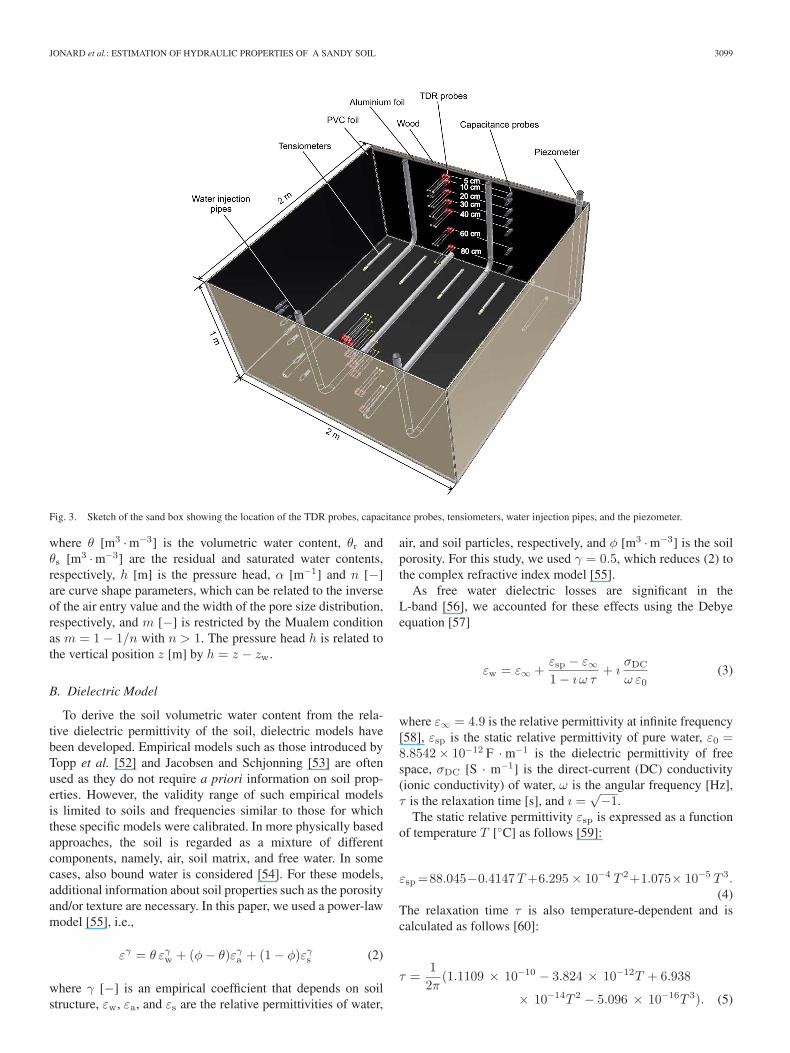
TDR andcapacitance sensors were installed at seven differentdepths, i.e., 5, 10, 20, 30, 40, 60, and 80 cm, below the sand sur-face at two opposite sides of the sand box to measure profiles ofthe relative dielectric permittivity, i.e., ε, and bulk electrical con-ductivity, i.e.,σ (see Fig. 3). TDR measurements were carried outevery 20 min using homemade three-rod probes with a length of20 cm that were inserted horizontally into the sand. TDR probeswere connected to a TDR100 cable tester and a CR1000 datalogger (both Campbell Scientific, Logan, Utah, USA). The TDRwaveforms were analyzed using the tangent method in the timedomain [47]. Bulk soil electrical conductivity and soil tempera-ture measurements were carried out every 15 min using 5TEcapacitance sensors (Decagon Devices, Inc., Pullman, Wash-ington, USA) composed of three prongs of 5.2-cm length,also inserted horizontally into the sand. Furthermore, a piezo-meter was used to monitor the water table depth (see Fig. 3).

C. Remote Sensing Systems

1) L-Band Radiometer: We used the L-band radiometerELBARA-II [48], which is the same instrument as those usedby ESA for calibration and validation activities of the SMOSmission. The ELBARA-II radiometer is sensitive within theprotected frequency band 1400–1427 MHz of the microwaveL-band. The internal noise reference sources used to achievecalibrated brightness temperature were realized with a hotresistive noise source (at about 313 K) and an active coldsource (at about 40 K). Furthermore, the noise power at theradiometer input ports was corrected for the noise added bythe lossy feed cables (about 0.2 dB) assumed to be at theair temperature. A detailed description of the ELBARA-IIsystem and of the applied calibration procedure is providedby Schwank et al. [48]. Each day when measurements wereperformed, the radiometer was calibrated by measuring skyradiance at an elevation angle of about 55◦ above the horizonand oriented approximately toward the north. Each radiometermeasurement was performed with a 3-s integration time toachieve an absolute accuracy better than 1 K [49]. The ra-diometer was equipped with a dual-mode conical horn antenna(aperture diameter = 60 cm, length = 67 cm) with symmetri-cal and identical beams and a −3-dB full beamwidth of 23◦

in the far field. The antenna directivity was derived from thetime series of brightness temperatures measured with the sunpassing through the antenna field of view [48].

2) Ground-Penetrating Radar: The radar measurementswere carried out using an ultrawideband stepped-frequencycontinuous-wave radar [37], [50]. The radar system was setup using a vector network analyzer (VNA, ZVRE, Rohde& Schwarz, Munich, Germany) connected to a transmittingand receiving linear polarized double-ridged broadband hornantenna (BBHA 9120 A, Schwarzbeck Mess-Elektronik,Schönau, Germany). The antenna was connected to thereflection port of the VNA with a low-loss N-type 50-ohmimpedance coaxial cable. Before each measurement, the VNAwas calibrated at the connection between the coaxial cable andthe antenna using a standard open-short-match calibration kit.The antenna has a length of 22 cm and a 14 × 25 cm2 aperturearea. Its −3-dB full beamwidth is 26◦ in the E-plane and 20◦ inthe H-plane (at 2 GHz). The antenna nominal frequency rangeis 0.8–5.2 GHz and its isotropic gain ranges from 4.4–14 dBi.Measurements were performed between 0.8–2.6 GHz with afrequency step of 8 MHz.

III. MODELING APPROACH

A. Soil Hydraulic Model

Radiometer and radar measurements were performed whenthe sand was in hydrostatic equilibrium with a water tablelocated at position zw [m]. In hydrostatic equilibrium, the watercontent profile follows the water retention curve of the soil,which we described using the van Genuchten model [51], i.e.,

θ(h) =

{θr + (θs − θr) [1 + |αh|n]−m for h < 0

θs for h ≥ 0(1)

JONARD et al.: ESTIMATION OF HYDRAULIC PROPERTIES OF A SANDY SOIL 3099

Fig. 3. Sketch of the sand box showing the location of the TDR probes, capacitance probes, tensiometers, water injection pipes, and the piezometer.

where θ [m3 ·m−3] is the volumetric water content, θr andθs [m3 ·m−3] are the residual and saturated water contents,respectively, h [m] is the pressure head, α [m−1] and n [−]are curve shape parameters, which can be related to the inverseof the air entry value and the width of the pore size distribution,respectively, and m [−] is restricted by the Mualem conditionas m = 1− 1/n with n > 1. The pressure head h is related tothe vertical position z [m] by h = z − zw.

B. Dielectric Model

To derive the soil volumetric water content from the rela-tive dielectric permittivity of the soil, dielectric models havebeen developed. Empirical models such as those introduced byTopp et al. [52] and Jacobsen and Schjonning [53] are oftenused as they do not require a priori information on soil prop-erties. However, the validity range of such empirical modelsis limited to soils and frequencies similar to those for whichthese specific models were calibrated. In more physically basedapproaches, the soil is regarded as a mixture of differentcomponents, namely, air, soil matrix, and free water. In somecases, also bound water is considered [54]. For these models,additional information about soil properties such as the porosityand/or texture are necessary. In this paper, we used a power-lawmodel [55], i.e.,

εγ = θ εγw + (φ− θ)εγa + (1− φ)εγs (2)

where γ [−] is an empirical coefficient that depends on soilstructure, εw, εa, and εs are the relative permittivities of water,

air, and soil particles, respectively, and φ [m3 ·m−3] is the soilporosity. For this study, we used γ = 0.5, which reduces (2) tothe complex refractive index model [55].

As free water dielectric losses are significant in theL-band [56], we accounted for these effects using the Debyeequation [57]

εw = ε∞ +εsp − ε∞1− ı ω τ

+ ıσDC

ω ε0(3)

where ε∞ = 4.9 is the relative permittivity at infinite frequency[58], εsp is the static relative permittivity of pure water, ε0 =8.8542× 10−12 F · m−1 is the dielectric permittivity of freespace, σDC [S · m−1] is the direct-current (DC) conductivity(ionic conductivity) of water, ω is the angular frequency [Hz],τ is the relaxation time [s], and ı =

√−1.

The static relative permittivity εsp is expressed as a functionof temperature T [◦C] as follows [59]:

εsp=88.045−0.4147T+6.295× 10−4 T 2+1.075× 10−5 T 3.(4)

The relaxation time τ is also temperature-dependent and iscalculated as follows [60]:

τ =1

2π(1.1109 × 10−10 − 3.824 × 10−12T + 6.938

× 10−14T 2 − 5.096 × 10−16T 3). (5)

3100 IEEE TRANSACTIONS ON GEOSCIENCE AND REMOTE SENSING, VOL. 53, NO. 6, JUNE 2015

C. Microwave Emission Model (Radiometer)

The first part of this section describes the model used toderive the reflectivities Rp

s of the sand box from the brightnesstemperatures T p

B measured with the L-band radiometer. Thesubsequent part of this section outlines the approach used torelate sand box reflectivities Rp

s to water content profiles.1) Brightness Temperatures: The thermal L-band emission,

also called brightness temperature, T pB, is expressed with a RT

model that fulfills Kirchhoff’s law (e.g., [16]). To include bothradiance emitted from the sand box and from the surroundingarea, T p

B at horizontal (p = H) and vertical (p = V) polariza-tion is represented as a corresponding linear combination, i.e.,

T pB = ηp [(1−Rp

s )Ts +Rps Tsky]

+ (1− ηp) [(1−Rp0)T0 +Rp

0 Tsky] . (6)

The weighting factor ηp is used to express the fractionalamounts of radiance emitted from the sand box (ηp) and thesurrounding area covered with the wire grid (1− ηp).

Rps [−] and Rp

0 [−] are the reflectivities of the sand boxand the surrounding area, respectively. At thermal equilibrium,(1−Rp

s ) and (1−Rp0) represent the corresponding emissiv-

ities. The downwelling sky radiance reflected at the groundis assumed to be Tsky = 4.8K [61]. Ts [K] and T0 [K] arethe effective physical temperatures of the filled sand box andthe surrounding area, respectively. In this paper, Ts was ap-proximated as the arithmetic mean of the sand temperaturesmeasured at depths of 5 and 40 cm. T0 was approximated bythe air temperature measured near the radiometer feed point.

The weighting factor ηp used in (6) is computed from the nor-malized antenna directivity D(Θ) = exp(−0.005309Θ2) withΘ(x, y) being the polar angle between the main direction ofthe antenna and the position of a facet with coordinates (x, y)within the footprint plane

η =

∫ ∫A

D(Θ(x, y)) dΩ(x, y, dx, dy). (7)

This integral is evaluated numerically over area A of thesand box, with dΩ(x, y, dx, dy) [rad] being the solid anglesof footprint facets with infinitesimal areas dxdy. Consideringall the dimensions depicted in Fig. 1(b), the evaluation of(7) yields η = 0.48. It is worth noting that η in (7) does notdepend on polarization p as the antenna directivity D(Θ) canbe considered as polarization independent for the symmetricalPicket horn antenna. The value of ηp = 0.48 in (6) allows usto derive the reflectivities Rp

0 of the surrounding area from T pB

measured with the sand box covered with a copper sheet actingas a reflector with Rp

s,ref = 1. Solving (6) with ηp = 0.48 andRH

s,ref = RVs,ref = 1 yielded RH

0 = 0.95 and RV0 = 0.92.

Alternatively, the weighting factor ηp and the effective re-flectivity Rp

0 of the area outside the sand box are derived from(6) without a priori information on the antenna directivity.To this end, T p

B was measured for two different footprintconfigurations: 1) the area A = 4m2 of the sand box is coveredwith a reflector (copper sheet); and 2) the sand box is cov-

Fig. 4. Three-dimensional planar layered medium with a radar point sourceand receiver or a radiometer point receiver (S). Each layer is characterized bythe dielectric permittivity εn, electric conductivity σn, magnetic permeabilityμn, and thickness hn.

ered with a microwave absorber (EPP22, Telemeter Elektronic,Donauwörth, Germany). The attenuation of the absorber isspecified as −30 dB at the microwave L-band. Accordingly,the reflectivity of the absorber is assumed to be Rp

s,abs = 0.Considering the T p

B measured for the configurations (1) and(2) with associated reflectivities Rp

s = Rps,ref = 1 and Rp

s =

Rps,abs = 0 in (6) yields two equations for the two unknowns

ηp and Rp0. Solving these two equations (each with p = H or

V) for the two unknowns yielded ηH = ηV = 0.54 and RH0 =

0.94, RV0 = 0.90. Although the results derived from the two

approaches were very similar, we considered the model-basedvalues ηp = 0.48, RH

0 = 0.95, and RV0 = 0.92 derived from

the antenna directivity. This choice was based on the fact thatthe antenna directivity is considered to be more reliable than theassumption Rp

s,abs = 0, which is crucial for the experimentalapproach. Finally, sand box reflectivities Rp

s can be derivedfrom T p

B measurements carried out for the uncovered sand box.2) Reflectivities: Reflectivities Rp

s of the sand box canbe modeled based on sand permittivity data using differentapproaches. A rather simple approach is to assume a con-stant water content along the sand depth. However, a moresophisticated approach is required to model Rp

s in order toaccount for the water retention curve profiles dealt with inthis study. To this end, a coherent RT model [62], applicableto planar layered dielectric media, was used. This model isvery efficient in terms of computation time as it uses a matrixformulation of the boundary conditions at the layer interfacesderived from Maxwell’s equations. This is important in view ofthe fine discretization required to represent smooth dielectricprofiles realistically across the sand depth. Accordingly, Rp

s

were computed with the coherent RT model evaluated for Ndielectric layers (distinguished by subscript n = 1, 2, . . . , N )with thickness hn = 0.5 cm, which corresponds to one-tenth ofthe minimum wavelength in the medium in order to emulateprofile continuity [63]. As depicted in Fig. 4, each layer ischaracterized by its dielectric permittivity εn and its electricalconductivity σn. The magnetic permeability (μn) is consideredconstant and equal to the permeability of free space (μ0 =4π10−7 H · m−1). To derive the reflectivities Rp

s of the layer

JONARD et al.: ESTIMATION OF HYDRAULIC PROPERTIES OF A SANDY SOIL 3101

stack, the sand permittivity profiles and the related water con-tent profiles were simulated using the van Genuchten model[see (1)].

D. GPR Model

The first part of this section describes the radar equation usedto derive Green’s functions G↑

xx(ω) from off-ground GPR mea-surements. Here, G↑

xx(ω) represents the backscattered electricfield from the sand box normalized to a unit-strength electricsource. In the second part of this section, we introduce theapproach used to simulate the medium response, namely,Green’s function G↑

xx(ω), based on permittivity profileinformation.

1) Radar Equation: The radar measurements (raw data)S11(ω) can be expressed as the ratio between the backscatteredelectromagnetic field b(ω) and the incident electromagneticfield a(ω) at the VNA calibration plane, with ω being the an-gular frequency. In far-field conditions, the spatial distributionof the backscattered electromagnetic field over the antennaaperture can be assumed to be independent of the layeredmedium, i.e., only the phase and amplitude of the field change(homogeneous field over the antenna aperture). In this case, thefollowing radar equation, expressed in the frequency domain,can be used to describe the radar raw data [37]

S11(ω) =b(ω)

a(ω)= Hi(ω) +

H(ω)G↑xx(ω)

1−Hf(ω)G↑xx(ω)

(8)

where S11(ω) is the international standard quantity measuredby the VNA, Hi(ω) is the global reflection coefficient of theantenna for the fields incident from the VNA calibration planeonto the point source (corresponding to the free space responseof the antenna), H(ω) = Ht(ω)Hr(ω) where Ht(ω) is theglobal transmission coefficient for fields incident from the VNAcalibration plane onto the point source, Hr(ω) is the globaltransmission coefficient for fields incident from the field pointonto the VNA calibration plane, Hf(ω) is the global reflectioncoefficient for the field incident from the layered medium ontothe field point, and G↑

xx(ω) is the planar layered mediumGreen’s function.

The global reflection and transmission coefficients [Hi(ω),H(ω), and Hf(ω)] were determined by solving a system ofequations [see (8)] for different model configurations. We usedseveral well-defined configurations with the antenna at differentheights above a copper plane functioning as an infinite perfectelectrical conductor. Once the antenna characteristic functionsare known, antenna effects can be filtered out from the radarmeasurements, i.e., Green’s functions can be derived from theS11(ω) measurements.

2) Green’s Functions: The radar model used to simulateGreen’s functions G↑

xx(ω) consists of a 3-D planar layeredmedium (N horizontal layers) with a point source and receiver(see Fig. 4). The use of a 3-D model is essential to take intoaccount spherical divergence (geometric spreading) in wavepropagation. The medium of the nth layer is assumed to behomogeneous and can be characterized by a single dielec-tric permittivity εn, an electrical conductivity σn, a magnetic

permeability μn = μ0, and a thickness hn = 0.5 cm. Green’sfunction, formulated as an exact solution of the 3-D Maxwellequations for electromagnetic waves propagating in planar lay-ered media, is derived by computing, with a recursive scheme,the transverse electric (TE) and magnetic (TM) global reflec-tion coefficients of the planar layered medium in the spectraldomain [64]. The transformation back to the spatial domain isperformed by numerically evaluating a semi-infinite complexintegral [65].

E. Bayesian Inversion Scheme

A coupled electromagnetic and hydrological inversion of theGPR and the radiometer data was performed to estimate thehydraulic parameters (θr, θs, α, and n) of the van Genuchtenmodel. The saturated water content θs was used as a fixedparameter and was set to the value derived from the estimatedsand porosity (see below). It is worth noting that θs can be ex-perimentally obtained from radar or radiometer measurementswhen the soil surface is fully saturated. However, it was notpossible to saturate the sand surface during the experiment dueto technical constraints. Water table levels zw were measured,and, therefore, considered as a known parameter for the in-versions. The parameter space considered for the three freeparameters θr, α, and n involved in the inversions was definedas [0 ≤ θr ≤ 0.10m3 · m−3; 1 ≤ α ≤ 20m−1; 1.1 ≤ n ≤ 10].

The optimal values of the model parameters and their uncer-tainties were estimated using a Bayesian inversion method, asimplemented in the DiffeRential Evolution Adaptive Metropo-lis (DREAM) algorithm. DREAM is a Markov chain MonteCarlo sampler that can be used to efficiently estimate theposterior probability distribution of the model parameters fornonlinear problems [46]. After convergence, the last 5000 sam-ples were used to represent the posterior parameter distribution.

Under the assumption of independent and identically dis-tributed Gaussian error residuals, the likelihood function (L),which represents, in probabilistic sense, the overall distance be-tween the model simulations and corresponding observations,can be simply defined as follows [66]:

log(L) ∝ −Nobs

2log(SSR) (9)

where Nobs is the number of observations. In order to solvethe inverse problem, the log-likelihood [see (9)] is maximizedusing the global optimization algorithm DREAM. SSR, thesum of squared residuals, is defined according to the sens-ing method considered. For the off-ground GPR, SSR isdefined as

SSRGPR(b) =∣∣G↑∗

xx −G↑xx

∣∣T ∣∣G↑∗xx −G↑

xx

∣∣ (10)

where G↑∗xx = G↑∗

xx(ω, zw) and G↑xx = G↑

xx(ω, zw,b) are, re-spectively, the measured and modeled complex Green’s func-tions in the frequency domain [antenna effects are removedusing (8)], b = [θr, α, n] is the parameter vector to be es-timated. To further reduce the dimensionality of the inverseproblem, the distance between the sand surface and the GPR

3102 IEEE TRANSACTIONS ON GEOSCIENCE AND REMOTE SENSING, VOL. 53, NO. 6, JUNE 2015

Fig. 5. Water content profiles for seven water table depths zw. Solid lines represent the sand water retention curve estimated using all TDR data simultaneously.Markers represent TDR measurements, for the two different profiles (red circles and blue triangles). Horizontal dashed lines represent the water table levels. Notethat TDR measurements at 0.80 m depth were not taken into consideration when fitting the water retention curve.

antenna phase center h0 [m] (see Fig. 4) was previously esti-mated by performing inversion of the electromagnetic modelin the time domain [34], [35]. The height h0 was then used as afixed parameter for the inversion. For the microwave radiometer(MR), SSR is defined as

SSRMR(b) = (R∗s −Rs)

T (R∗s −Rs) (11)

where R∗s = R∗

s(p, zw) and Rs = Rs(p, zw,b) are, respec-tively, the measured and modeled reflectivities, and b =[θr, α, n, η] is the parameter vector to be estimated. Note thatthe weighting factor η used in (6) was also retrieved. Thesand hydraulic parameters were also estimated based on TDR-derived relative dielectric permittivities. In this case, SSR isdefined as

SSRTDR(b) = (ε∗ − ε)T (ε∗ − ε) (12)

where ε∗=ε∗(zTDR, zw) and ε=ε(zTDR, zw,b) are, respec-tively, the measured and modeled relative dielectric permittivityvectors, b=[θs, θr, α, n] is the parameter vector to be estimated,and zTDR is the depth of the TDR sensors. Here, θs was esti-mated and not used as a fixed parameter because several TDRsensors were also located in the saturated zone (the number ofTDR sensors depended on the actual water table depth).

IV. RESULTS AND DISCUSSION

A. In Situ TDR Data

We considered sand water content measured with TDR at thetime of radar and radiometer measurements for the inversion.However, continuous TDR measurements were taken to analyzethe behavior of the in situ sensors and to confirm the hydrostaticequilibrium of the sand box at the times of the remote measure-ments. The water table levels zw measured with a piezometer at

hydrostatic equilibrium were at zw=0.86m on DOY 294, zw=0.57m on DOY 304, zw=0.50m on DOY 311, zw=0.41m onDOY 319, zw=0.30m on DOY 325, zw=0.18m on DOY 332,and zw=0.17m on DOY 343.

TDR-derived volumetric water content values θ are plottedin Fig. 5 for the seven measured water table depths zw. Each θdata shown consists of a mean of six measurements. It shouldbe noted that similar water content values were observed forthe two measurement profiles located at the two sides of thesand box (mean standard deviation (STD) of 0.016 m3 ·m−3)indicating a rather homogeneous sand along the horizontaldirection (see Fig. 3). The sand water retention curve was fittedto the data according to (1) and (12), whereby only a singleretention curve was fitted to all TDR data without consideringthe data collected at a depth of 0.80 m. These water contentvalues were omitted as they show substantially higher valuescompared with all other TDR readings at saturation, suggestingmeasurement errors.

B. Brightness Temperatures

Fig. 6 shows brightness temperatures (T pB) measured with

the L-band radiometer at horizontal and vertical polariza-tion above the experimental setup (sand box + surroundingwire grid). The radiometer measurements were performed forthree different configurations, i.e., with the open sand surface(T p

B,sand+grid), with the sand surface covered by a microwaveabsorber (T p

B,abs+grid), and with the sand surface coveredby a perfect reflector (T p

B,ref+grid). Each T pB,sand+grid value

corresponds to a mean of at least 20 measurements performedfor 45 min. The STD of the repeated T p

B,sand+grid measure-ments is systematically smaller than 0.3 K, which confirmsthe repeatability of the measurements. T p

B,sand+grid decreaseswith increasing water table level zw from 150 K to 112 K for

JONARD et al.: ESTIMATION OF HYDRAULIC PROPERTIES OF A SANDY SOIL 3103

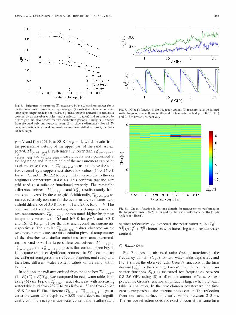
Fig. 6. Brightness temperature TB measured by the L-band radiometer abovethe free sand surface surrounded by a wire grid (triangles) as a function of watertable depth (depth scale is not linear). TB measurements above the sand surfacecovered by an absorber (circles) and a reflector (squares) and surrounded bya wire grid are also shown for two calibration periods. Finally, TB emittedfrom the sand only and retrieved using (6) is shown (diamonds). For all TB

data, horizontal and vertical polarizations are shown (filled and empty markers,respectively).

p = V and from 138 K to 88 K for p = H, which results fromthe progressive wetting of the upper part of the sand. As ex-pected, TH

B,sand+grid is systematically lower than TVB,sand+grid.

T pB,ref+grid and T p

B,abs+grid measurements were performed atthe beginning and in the middle of the measurement campaignto characterize the setup. T p

B,ref+grid measured above the sandbox covered by a copper sheet shows low values (14.9–16.9 Kfor p = V and 11.9–12.2 K for p = H) comparable to the skybrightness temperature (≈4.8 K). This confirms that the wiregrid used as a reflector functioned properly. The remainingdifference between T p

B,ref+grid and T psky results mainly from

areas not covered by the wire grid. Additionally, T pB,ref+grid re-

mained relatively constant for the two measurement dates, witha slight difference of 0.3 K for p = H and 2.0 K for p = V. Thisconfirms that the setup did not significantly change between thetwo measurements. T p

B,abs+grid shows much higher brightnesstemperature values with 169 and 167 K for p=V and 163 Kand 161 K for p=H for the first and second measurements,respectively. The similar T p

B,abs+grid values observed on thetwo measurement dates are due to similar physical temperaturesof the absorber and similar emissions from areas surround-ing the sand box. The large differences between T p

B,ref+grid,T pB,abs+grid, and T p

B,sand+grid proves that our setup (see Fig. 1)is adequate to detect significant contrasts in T p

B measured forthe different configurations (reflector, absorber, and sand) and,therefore, different water content values of the sand withinthe box.

In addition, the radiance emitted from the sand box T pB,sand=

(1−Rps )Ts+Rp

s Tsky was computed for each water table depthusing (6) (see Fig. 6). T p

B,sand values decrease with increasingwater table level from 282 K to 203 K for p=V and from 266 to163 K for p=H. The difference T p

B,sand−T pB,sand+grid is great-

est at the water table depth zw=0.86m and decreases signifi-cantly with increasing surface water content and resulting sand

Fig. 7. Green’s function in the frequency domain for measurements performedin the frequency range 0.8–2.6 GHz and for two water table depths, 0.57 (blue)and 0.17 m (green), respectively.

Fig. 8. Green’s function in the time domain for measurements performed inthe frequency range 0.8–2.6 GHz and for the seven water table depths (depthscale is not linear).

surface reflectivity. As expected, the polarization ratio (TVB −

THB )/(TV

B + THB ) increases with increasing sand surface water

content.

C. Radar Data

Fig. 7 shows the observed radar Green’s functions in thefrequency domain (G↑

xx) for two water table depths zw, andFig. 8 shows the observed radar Green’s functions in the timedomain (g↑xx) for the seven zw. Green’s function is derived fromscatter functions S11(ω) measured for frequencies between0.8–2.6 GHz using (8) to filter out antenna effects. As ex-pected, the Green’s function amplitude is larger when the watertable is shallower. In the time-domain counterpart, the timezero corresponds to the antenna phase center. The reflectionfrom the sand surface is clearly visible between 2–3 ns.The surface reflection does not exactly occur at the same time

3104 IEEE TRANSACTIONS ON GEOSCIENCE AND REMOTE SENSING, VOL. 53, NO. 6, JUNE 2015

TABLE IESTIMATED HYDRAULIC PARAMETERS FROM LABORATORY, TDR,

RADIOMETER, AND GPR MEASUREMENTS AND THEIR 2.5%, 50%, AND

97.5% PERCENTILE VALUES OBTAINED USING DREAM. THE LOWER

AND UPPER BOUNDS DEFINE THE PARAMETER SPACES CONSIDERED

FOR THE ESTIMATION OF THE HYDRAULIC PARAMETERS

for each measurement, as the height of the antenna was slightlydifferent for the different measurements (0.35–0.40 m). Theamplitude of the reflection increases with increasing water tablelevel as a consequence of the increased dielectric gradientbetween the free-space layer and the surface-sand layer (seeFig. 4). The remaining oscillations in the time-domain signalare aliasing effects caused by the band-limited (0.8–2.6 GHz)inverse Fourier transform. No clear reflection can be observedbelow the surface reflection, and the water table interfaceis not detectable either. This means that the sand dielectricprofile is rather smooth and without sharp transitions for thefrequencies used and that the electromagnetic waves are almosttotally attenuated in the capillary fringe and saturated zone. Theassumption of a smooth dielectric profile for the unsaturatedzone and an infinite lower half-space for the saturated zone inthe electromagnetic model can therefore be confirmed.

D. Soil Hydraulic Parameters and Water Retention Curve

The soil moisture profiles were reconstructed from the threefield measurement techniques, namely, TDR, radiometer, andoff-ground GPR, and the related hydraulic parameters of thevan Genuchten model [see (1)] were estimated. The referencelaboratory-derived hydraulic parameters, as well as the esti-mated hydraulic parameters from TDR, radiometer, and GPRand their 95% corresponding confidence intervals are presentedin Table I.

In the laboratory, soil hydraulic parameters are classicallyderived by fitting the van Genuchten model to retention data ob-tained from hydrostatic column experiments (see Section II-A).However, for the coarse-textured sand used in our experiment,the pores are relatively large and the air entrance value is

smaller than the height of the samples used in the laboratory.Therefore, parts of the column cannot be saturated at thebeginning of the laboratory experiment. Consequently, datarecorded at the first pressure steps are unreliable and θs cannotbe accurately estimated [3], [4]. Laboratory data at the first twopressure steps (−1 and −5 cm) were then not considered for theestimation of the hydraulic parameters. Alternatively, θs can beestimated from its porosity φ = θs expressed with

φ = 1− ρbulk/ρs (13)

where ρbulk [g · cm−3] is the bulk density measured from undis-turbed samples (ρbulk = 1.64 g · cm−3) and ρs [g · cm−3] is thesoil particle density, which is assumed to be ρs = 2.62 g · cm−3

for a quartz sand. The value obtained is θs = 0.37m3 · m−3,which is similar to the value derived from TDR data (θs =0.36m3 · m−3). As already mentioned, θs was not estimatedfrom radiometer and radar measurements, as saturated condi-tions at the soil surface could not be attained in the sand box.Estimation of the hydraulic parameters from radiometer andradar data were therefore performed by constraining θs to thevalue derived from the estimated porosity [see (13)].

Table I shows that the radiometer- and GPR-derived θr valuesare equal to 0 such as the reference laboratory-derived θr,whereas TDR-derived θr is equal to 0.03 m3 ·m−3. GPR- andTDR-derived α show similar values, whereas the α estimatefrom radiometer is slightly smaller. In addition, the laboratory-derived α value is significantly higher compared with that de-rived from the three other techniques. The estimated values forn are similar when derived from the field techniques, whereasthe laboratory-derived n value is significantly smaller.

In general, the confidence intervals for the estimated param-eters are significantly smaller for GPR (0.002 m3 ·m−3 for θr,0.63 m−1 for α, and 0.67 for n) compared with TDR (0.045 m3 ·m−3 for θr, 0.92 m−1 for α, and 1.86 for n), radiome-ter (0.063 m3 ·m−3 for θr, 1.94 m−1 for α, and 2.44 forn), and the laboratory measurements (0.049 m3 ·m−3 for θr,3.03 m−1 for α, and 0.52 for n), except for the confidenceinterval for n, which is slightly smaller for the laboratorymeasurements. The smaller confidence intervals of the GPR-derived parameters could be explained by the larger amountof information contained in the GPR data (226 frequen-cies) compared with the TDR (2 × 7 positions) and theradiometer data (2 polarizations). In addition, the lower fre-quencies of the GPR provide information for greater depthscompared with the radiometer. It is worth noting that thehigh accuracy of the GPR electromagnetic model for theconfiguration used (e.g., homogeneous sand box, smooth soilsurface, no vegetation cover) could also lead to relatively smallconfidence intervals for the estimates.

Parameter η, which is the fractional amount of the measuredradiance emitted from the sand box, was also estimated fromradiometer data simultaneously with the hydraulic parameters.The estimated value of η is 0.50 with a 95% confidence intervalof [0.49 0.54]. This value is similar to that obtained fromthe antenna characterization (η = 0.48) and the absorber andreflector measurements (η = 0.54).

JONARD et al.: ESTIMATION OF HYDRAULIC PROPERTIES OF A SANDY SOIL 3105

Fig. 9. Marginal posterior probability distribution of the model parametersestimated by the different methods (laboratory, TDR sensors, radiometer,and GPR). Parameter distributions are obtained using the last 5000 samplesgenerated with DREAM.

TABLE IICORRELATIONS BETWEEN THE ESTIMATED HYDRAULIC PARAMETERS

FROM TDR, RADIOMETER, AND GPR MEASUREMENTS

To gain more information about the parameter uncertainties,the marginal posterior distribution of the model parametersestimated by the different techniques is plotted in Fig. 9. Theparameter distributions are obtained using the last 5000 samplesgenerated with DREAM. As can be seen, very narrow confi-dence intervals are obtained for the GPR-derived parameters(θr, α, and n) and n derived in the laboratory.

Table II shows the correlation between the hydraulic pa-rameters for the three measurement techniques applied tothe sand box. The correlation between α and n is large forthe GPR inversion, whereby a general correlation betweenthese two parameters has already been detected in variouspublications [5], [67]–[69]. Hardly any correlation betweenthese two parameters can be found using TDR data. The cor-relation is intermediate for the radiometer-derived parameters.This can also be clearly observed in Fig. 10, which shows

Fig. 10. Response surfaces of the log-likelihood [see (9)] in the α–n parame-ter plane for the TDR (a), radiometer (b), and GPR (c) inversions. The asteriskrepresents the global maximum. Note that the color scale differs for the threeresponse surfaces.

3106 IEEE TRANSACTIONS ON GEOSCIENCE AND REMOTE SENSING, VOL. 53, NO. 6, JUNE 2015

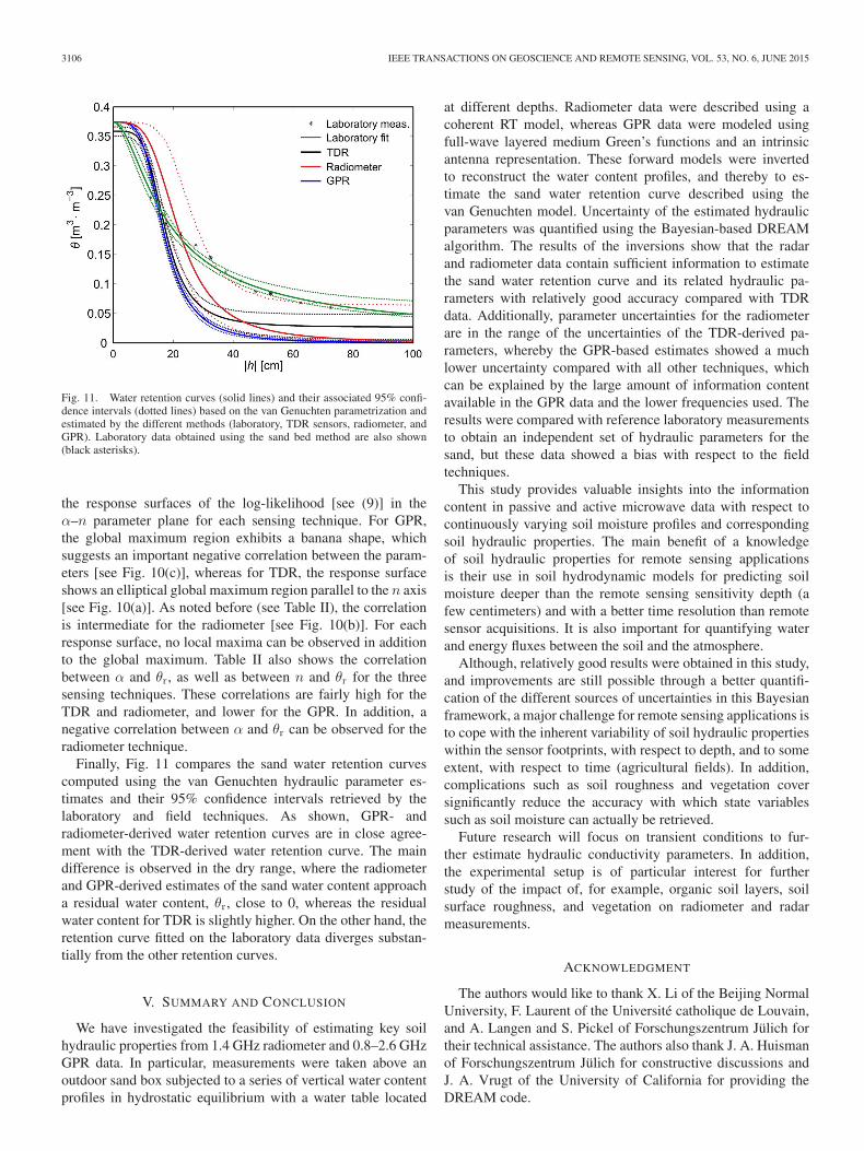
Fig. 11. Water retention curves (solid lines) and their associated 95% confi-dence intervals (dotted lines) based on the van Genuchten parametrization andestimated by the different methods (laboratory, TDR sensors, radiometer, andGPR). Laboratory data obtained using the sand bed method are also shown(black asterisks).

the response surfaces of the log-likelihood [see (9)] in theα–n parameter plane for each sensing technique. For GPR,the global maximum region exhibits a banana shape, whichsuggests an important negative correlation between the param-eters [see Fig. 10(c)], whereas for TDR, the response surfaceshows an elliptical global maximum region parallel to the n axis[see Fig. 10(a)]. As noted before (see Table II), the correlationis intermediate for the radiometer [see Fig. 10(b)]. For eachresponse surface, no local maxima can be observed in additionto the global maximum. Table II also shows the correlationbetween α and θr, as well as between n and θr for the threesensing techniques. These correlations are fairly high for theTDR and radiometer, and lower for the GPR. In addition, anegative correlation between α and θr can be observed for theradiometer technique.

Finally, Fig. 11 compares the sand water retention curvescomputed using the van Genuchten hydraulic parameter es-timates and their 95% confidence intervals retrieved by thelaboratory and field techniques. As shown, GPR- andradiometer-derived water retention curves are in close agree-ment with the TDR-derived water retention curve. The maindifference is observed in the dry range, where the radiometerand GPR-derived estimates of the sand water content approacha residual water content, θr, close to 0, whereas the residualwater content for TDR is slightly higher. On the other hand, theretention curve fitted on the laboratory data diverges substan-tially from the other retention curves.

V. SUMMARY AND CONCLUSION

We have investigated the feasibility of estimating key soilhydraulic properties from 1.4 GHz radiometer and 0.8–2.6 GHzGPR data. In particular, measurements were taken above anoutdoor sand box subjected to a series of vertical water contentprofiles in hydrostatic equilibrium with a water table located

at different depths. Radiometer data were described using acoherent RT model, whereas GPR data were modeled usingfull-wave layered medium Green’s functions and an intrinsicantenna representation. These forward models were invertedto reconstruct the water content profiles, and thereby to es-timate the sand water retention curve described using thevan Genuchten model. Uncertainty of the estimated hydraulicparameters was quantified using the Bayesian-based DREAMalgorithm. The results of the inversions show that the radarand radiometer data contain sufficient information to estimatethe sand water retention curve and its related hydraulic pa-rameters with relatively good accuracy compared with TDRdata. Additionally, parameter uncertainties for the radiometerare in the range of the uncertainties of the TDR-derived pa-rameters, whereby the GPR-based estimates showed a muchlower uncertainty compared with all other techniques, whichcan be explained by the large amount of information contentavailable in the GPR data and the lower frequencies used. Theresults were compared with reference laboratory measurementsto obtain an independent set of hydraulic parameters for thesand, but these data showed a bias with respect to the fieldtechniques.

This study provides valuable insights into the informationcontent in passive and active microwave data with respect tocontinuously varying soil moisture profiles and correspondingsoil hydraulic properties. The main benefit of a knowledgeof soil hydraulic properties for remote sensing applicationsis their use in soil hydrodynamic models for predicting soilmoisture deeper than the remote sensing sensitivity depth (afew centimeters) and with a better time resolution than remotesensor acquisitions. It is also important for quantifying waterand energy fluxes between the soil and the atmosphere.

Although, relatively good results were obtained in this study,and improvements are still possible through a better quantifi-cation of the different sources of uncertainties in this Bayesianframework, a major challenge for remote sensing applications isto cope with the inherent variability of soil hydraulic propertieswithin the sensor footprints, with respect to depth, and to someextent, with respect to time (agricultural fields). In addition,complications such as soil roughness and vegetation coversignificantly reduce the accuracy with which state variablessuch as soil moisture can actually be retrieved.

Future research will focus on transient conditions to fur-ther estimate hydraulic conductivity parameters. In addition,the experimental setup is of particular interest for furtherstudy of the impact of, for example, organic soil layers, soilsurface roughness, and vegetation on radiometer and radarmeasurements.

ACKNOWLEDGMENT

The authors would like to thank X. Li of the Beijing NormalUniversity, F. Laurent of the Université catholique de Louvain,and A. Langen and S. Pickel of Forschungszentrum Jülich fortheir technical assistance. The authors also thank J. A. Huismanof Forschungszentrum Jülich for constructive discussions andJ. A. Vrugt of the University of California for providing theDREAM code.

JONARD et al.: ESTIMATION OF HYDRAULIC PROPERTIES OF A SANDY SOIL 3107

REFERENCES

[1] A. K. Betts, J. H. Ball, A. C. M. Beljaars, M. J. Miller, and P. A. Viterbo,“The land surface-atmosphere interaction: A review based on obser-vational and global modeling perspectives,” J. Geophys. Res., Atmos.,vol. 101, no. D3, pp. 7209–7225, Mar. 1996.

[2] R. D. Koster et al., “Regions of strong coupling between soil moisture andprecipitation,” Science, vol. 305, no. 5687, pp. 1138–1140, Aug. 2004.

[3] A. Peters and W. Durner, “Improved estimation of soil water retentioncharacteristics from hydrostatic column experiments,” Water Resour. Res.,vol. 42, no. 11, Nov. 2006, Art. ID. W11401.

[4] M. Bittelli and M. Flury, “Errors in water retention curves determinedwith pressure plates,” Soil Sci. Soc. Amer. J., vol. 73, no. 5, pp. 1453–1460,Sep. 2009.

[5] C. M. Mboh, J. A. Huisman, and H. Vereecken, “Feasibility of sequen-tial and coupled inversion of time domain reflectometry data to infersoil hydraulic parameters under falling head infiltration,” Soil Sci. Soc.Amer. J., vol. 75, no. 3, pp. 775–786, May 2011.

[6] D. L. Corwin, J. Hopmans, and G. H. de Rooij, “From field- to landscape-scale vadose zone processes: Scale issues, modeling, and monitoring,”Vadose Zone J., vol. 5, no. 1, pp. 129–139, Jan. 2006.

[7] H. Vereecken, R. Kasteel, J. Vanderborght and T. Harter, “Upscalinghydraulic properties and soil water flow processes in heterogeneous soils:A review,” Vadose Zone J., vol. 6, no. 1, pp. 1–28, Feb. 2007.

[8] J. H. M. Wösten, Y. A. Pachepsky, and W. J. Rawls, “Pedotransfer func-tions: Bridging gap between available basic soil data and missing soilhydraulic characteristics,” J. Hydrol., vol. 251, no. 3/4, pp. 123–150,2001.

[9] H. Vereecken et al., “Using pedotransfer functions to estimate the vanGenuchten-Mualem soil hydraulic properties: A review,” Vadose Zone J.,vol. 9, no. 4, pp. 795–820, Nov. 2010.

[10] M. G. Schaap, “Accuracy and uncertainty in PTF predictions” inDevelopment of Pedotransfer Functions in Soil Hydrology, vol. 30,Y. P. Rawls and W. J., Eds. Amsterdam, The Netherlands: Elsevier,2004, pp. 33–43.

[11] H. L. Deng, M. Ye, M. G. Schaap, and R. Khaleel, “Quantification ofuncertainty in pedotransfer function-based parameter estimation for un-saturated flow modeling,” Water Resour. Res., vol. 45, no. 4, Apr. 2009,Art. ID. W04409.

[12] F. T. Ulaby, M. K. Moore, and A. K. Fung, Microwave Remote Sensing:Active and Passive, vol. I, Fundamentals and Radiometry. Reading, MA,USA: Addison-Wesley, 1981.

[13] F. T. Ulaby, M. K. Moore, and A. K. Fung, Microwave Remote Sensing:Active and Passive, vol. II, Radar Remote Sensing and Surface Scatteringand Emission Theory. Norwood, MA, USA: Artech House, 1982.

[14] F. T. Ulaby, M. K. Moore, and A. K. Fung, Microwave Remote Sensing:Active and Passive, vol. III, From Theory to Applications. Norwood,MA, USA: Artech House, 1986.

[15] T. J. Schmugge, W. P. Kustas, J. C. Ritchie, T. J. Jackson, and A. Rango,“Remote sensing in hydrology,” Adv. Water Resourc., vol. 25, no. 8–12,pp. 1367–1385, Aug. 2002.

[16] C. Mätzler, Thermal Microwave Radiation: Applications for RemoteSensing. London, U.K.: The Inst. Eng. Technol., 2006, ser. IETElectromagnetic Waves series 52.

[17] W. Wagner et al., “Operational readiness of microwave remote sensing ofsoil moisture for hydrologic applications,” Nordic Hydrol., vol. 38, no. 1,pp. 1–20, 2007.

[18] J. C. Shi et al., “Progresses on microwave remote sensing of land sur-face parameters,” Sci. China–Earth Sci., vol. 55, no. 7, pp. 1052–1078,Jul. 2012.

[19] H. Vereecken, L. Weihermüller, F. Jonard, and C. Montzka, “Characteriza-tion of crop canopies and water stress related phenomena using microwaveremote sensing methods: A review,” Vadose Zone J., vol. 11, no. 2,May 2012.

[20] Y. H. Kerr et al., “Soil moisture retrieval from space: The Soil Moistureand Ocean Salinity (SMOS) mission,” IEEE Trans. Geosci. Remote Sens.,vol. 39, no. 8, pp. 1729–1735, Aug. 2001.

[21] Y. H. Kerr et al., “The SMOS mission: New tool for monitoringkey elements of the global water cycle,” Proc. IEEE, vol. 98, no. 5,pp. 666–687, May 2010.

[22] S. Mecklenburg et al., “ESA’s soil moisture and ocean salinity mission:Mission performance and operations,” IEEE Trans. Geosci. Remote Sens.,vol. 50, no. 5, pp. 1354–1366, May 2012.

[23] D. Entekhabi et al., “The Soil Moisture Active Passive (SMAP) mission,”Proc. IEEE, vol. 98, no. 5, pp. 704–716, May 2010.

[24] N. N. Das, D. Entekhabi, and E. G. Njoku, “An algorithm for mergingSMAP radiometer and radar data for high-resolution soil-moisture re-

trieval,” IEEE Trans. Geosci. Remote Sens., vol. 49, no. 5, pp. 1504–1512,May 2011.

[25] P. J. Camillo, P. E. Oneill, and R. J. Gurney, “Estimating soil hydraulicparameters using passive microwave data,” IEEE Trans. Geosci. RemoteSens., vol. GE-24, no. 6, pp. 930–936, Nov. 1986.

[26] E. J. Burke, R. J. Gurney, L. P. Simmonds, and P. E. O’Neill, “Usinga modeling approach to predict soil hydraulic properties from passivemicrowave measurements,” IEEE Trans. Geosci. Remote Sens., vol. 36,no. 2, pp. 454–462, Mar. 1998.

[27] N. M. Mattikalli, E. T. Engman, T. J. Jackson, and L. R. Ahuja,“Microwave remote sensing of temporal variations of brightness temper-ature and near-surface soil water content during a watershed-scale fieldexperiment, and its application to the estimation of soil physical proper-ties,” Water Resour. Res., vol. 34, no. 9, pp. 2289–2299, Sep. 1998.

[28] D. H. Chang and S. Islam, “Estimation of soil physical properties usingremote sensing and artificial neural network,” Remote Sens. Environ.,vol. 74, no. 3, pp. 534–544, Dec. 2000.

[29] J. A. Santanello et al., “Using remotely sensed estimates of soil moistureto infer soil texture and hydraulic properties across a semi-arid water-shed,” Remote Sens. Environ., vol. 110, no. 1, pp. 79–97, Sep. 2007.

[30] K. W. Harrison, S. V. Kumar, C. D. Peters-Lidard, and J. A. Santanello,“Quantifying the change in soil moisture modeling uncertainty from re-mote sensing observations using Bayesian inference techniques,” WaterResour. Res., vol. 48, no. 11, Nov. 2012, Art. ID. W11514.

[31] A. V. M. Ines and B. P. Mohanty, “Near-surface soil moistureassimilation for quantifying effective soil hydraulic properties usinggenetic algorithms: 2. Using airborne remote sensing duringSGP97 and SMEX02,” Water Resour. Res., vol. 45, no. 1, Jan. 2009,Art. ID. W01408.

[32] C. Montzka et al., “Hydraulic parameter estimation by remotely sensedtop soil moisture observations with the particle filter,” J. Hydrol., vol. 399,no. 2011, pp. 410–421, Mar. 2011.

[33] B. P. Mohanty, “Soil hydraulic property estimation using remote sensing:A review,” Vadose Zone J., vol. 12, no. 4, pp. 1–9, 2013.

[34] S. Lambot et al., “Analysis of air-launched ground-penetrating radar tech-niques to measure the soil surface water content,” Water Resour. Res.,vol. 42, no. 11, Nov. 2006, Art. ID. W11403.

[35] F. Jonard et al., “Mapping field-scale soil moisture with L-band radiome-ter and ground-penetrating radar over bare soil,” IEEE Trans. Geosci.Remote Sens., vol. 49, no. 8, pp. 2863–2875, Aug. 2011.

[36] J. Minet, P. Bogaert, M. Vanclooster, and S. Lambot, “Validation ofground penetrating radar full-waveform inversion for field scale soil mois-ture mapping,” J. Hydrol., vol. 424–425, pp. 112–123, Mar. 2012.

[37] S. Lambot, E. C. Slob, I. van den Bosch, B. Stockbroeckx, andM. Vanclooster, “Modeling of ground-penetrating radar for accuratecharacterization of subsurface electric properties,” IEEE Trans. Geosci.Remote Sens., vol. 42, no. 11, pp. 2555–2568, Nov. 2004.

[38] A. Klotzsche et al., “Full-waveform inversion of cross-hole ground-penetrating radar data to characterize a gravel aquifer close to the ThurRiver, Switzerland,” Near Surf. Geophys., vol. 8, no. 6, pp. 635–649,2010.

[39] S. Lambot and F. André, “Full-wave modeling of near-field radar data forplanar layered media reconstruction,” IEEE Trans. Geosci. Remote Sens.,vol. 52, no. 5, pp. 2295–2303, May 2014.

[40] A. Binley, G. Cassiani, R. Middleton, and P. Winship, “Vadose zoneflow model parameterisation using cross-borehole radar and resistivityimaging,” J. Hydrol., vol. 267, no. 3/4, pp. 147–159, Oct. 2002.

[41] D. F. Rucker and T. P. A. Ferré, “Parameter estimation for soil hydraulicproperties using zero-offset borehole radar: Analytical method,” Soil Sci.Soc. Amer. J., vol. 68, no. 5, pp. 1560–1567, Sep. 2004.

[42] M. B. Kowalsky et al., “Estimation of field-scale soil hydraulicand dielectric parameters through joint inversion of GPR andhydrological data,” Water Resour. Res., vol. 41, no. 11, Nov. 2005,Art. ID. W11425.

[43] M. Looms, A. Binley, K. H. Jensen, L. Nielsen, and T. M. Hansen, “Iden-tifying unsaturated hydraulic parameters using an integrated data fusionapproach on cross-borehole geophysical data,” Vadose Zone J., vol. 7,no. 1, pp. 238–248, Feb. 2008.

[44] S. Lambot et al., “Remote estimation of the hydraulic properties of asand using full-waveform integrated hydrogeophysical inversion of time-lapse, off-ground GPR data,” Vadose Zone J., vol. 8, no. 3, pp. 743–754,Aug. 2009.

[45] K. Z. Jadoon et al., “Estimation of soil hydraulic parameters in the field byintegrated hydrogeophysical inversion of time-lapse ground-penetratingradar data,” Vadose Zone J., vol. 11, no. 4, Nov. 2012.

[46] J. A. Vrugt et al., “Accelerating Markov Chain Monte Carlo simula-tion by differential evolution with self-adaptive randomized subspace

3108 IEEE TRANSACTIONS ON GEOSCIENCE AND REMOTE SENSING, VOL. 53, NO. 6, JUNE 2015

sampling,” Int. J. Nonlinear Sci. Numer. Simul., vol. 10, no. 3,pp. 273–290, Mar. 2009.

[47] T. J. Heimovaara and W. Bouten, “A computer-controlled 36-channel timedomain reflectometry system for monitoring soil-water contents,” WaterResour. Res., vol. 26, no. 10, pp. 2311–2316, Oct. 1990.

[48] M. Schwank et al., “ELBARA II, an L-band radiometer system for soilmoisture research,” Sensors, vol. 10, no. 1, pp. 584–612, Jan. 2010.

[49] M. Schwank et al., “L-band radiative properties of vine vegetation at theMELBEX III SMOS cal/val site,” IEEE Trans. Geosci. Remote Sens.,vol. 50, no. 5, pp. 1587–1601, May 2012.

[50] F. Jonard et al., “Characterization of tillage effects on the spatial variationof soil properties using ground-penetrating radar and electromagneticinduction,” Geoderma, vol. 207/208, pp. 310–322, Oct. 2013.

[51] M. T. van Genuchten, “A closed-form equation for predicting the hy-draulic conductivity of unsaturated soils,” Soil Sci. Soc. Amer. J., vol. 44,pp. 892–898, Sep. 1980.

[52] G. Topp, J. L. Davis, and A. P. Annan, “Electromagnetic determinationof soil water content: Measurements in coaxial transmission lines,” WaterResour. Res., vol. 16, no. 3, pp. 574–582, Jun. 1980.

[53] O. H. Jacobsen and P. Schjonning, “A laboratory calibration of time-domain reflectometry for soil-water measurement including effects ofbulk-density and texture,” J. Hydrol., vol. 151, no. 2–4, pp. 147–157,Nov. 1993.

[54] D. A. Robinson, S. B. Jones, J. M. Wraith, D. Or, and S. P. Friedman, “Areview of advances in dielectric and electrical conductivity measurementin soils using time-domain reflectometry,” Vadose Zone J., vol. 2, no. 4,pp. 444–475, Nov. 2003.

[55] K. Roth, R. Schulin, H. Flühler, and W. Attinger, “Calibration of time-domain reflectometry for water-content measurement using a compositedielectric approach,” Water Resour. Res., vol. 26, no. 10, pp. 2267–2273,Oct. 1990.

[56] T. J. Heimovaara, W. Bouten, and J. M. Verstraten, “Frequency domainanalysis of time domain reflectometry waveforms, 2, a four-componentcomplex dielectric mixing model for soils,” Water Resour. Res., vol. 30,no. 2, pp. 201–209, Feb. 1994.

[57] P. Debye, Polar Molecules. New York, NY, USA: Reinhold, 1929.[58] J. A. Lane and J. A. Saxton, “Dielectric dispersion in pure polar liquids

at very high radio frequencies. III. The effect of electrolytes in solution,”Proc. R. Soc. Lond. A, Math. Phys. Sci., vol. 214, no. 1119, pp. 531–545,Oct. 1952.

[59] L. A. Klein and C. T. Swift, “An improved model for the dielectricconstant of sea water at microwave frequencies,” IEEE Trans. AntennasPropag., vol. AP-25, no. 1, pp. 104–111, Jan. 1977.

[60] A. Stogryn, “Equations for calculating the dielectric constant of salinewater,” IEEE Trans. Microw. Theory Tech., vol. MTT-19, no. 8,pp. 733–736, Aug. 1971.

[61] T. Pellarin et al., “Two-year global simulation of L-band brightness tem-peratures over land,” IEEE Trans. Geosci. Remote Sens., vol. 41, no. 9,pp. 2135–2139, Sep. 2003.

[62] J. A. Dobrowolski, “Optical properties of films and coatings” in Hand-book of Optics, vol. I, M. Bass, E. W. Van Stryland, D. R. Williams, andW. L. Wolfe, Eds. New York, NY, USA: McGraw-Hill, 1995, pp. 42.

[63] S. Lambot, J. Rhebergen, I. van den Bosch, E. C. Slob, andM. Vanclooster, “Measuring the soil water content profile of a sandy soilwith an off-ground monostatic ground penetrating radar,” Vadose Zone J.,vol. 3, no. 4, pp. 1063–1071, Nov. 2004.

[64] E. C. Slob and J. Fokkema, “Coupling effects of two electric dipoles onan interface,” Radio Sci., vol. 37, no. 5, pp. 1073, 2002.

[65] S. Lambot, E. Slob, and H. Vereecken, “Fast evaluation of zero-offset Green’s function for layered media with application to ground-penetrating radar,” Geophys. Res. Lett., vol. 34, no. 21, Nov. 2007,Art. ID. L21405.

[66] B. Scharnagl, J. A. Vrugt, H. Vereecken, and M. Herbst, “Inverse mod-elling of in situ soil water dynamics: Investigating the effect of differentprior distributions of the soil hydraulic parameters,” Hydrol. Earth Syst.Sci., vol. 15, no. 10, pp. 3043–3059, 2011.

[67] J. A. Vrugt, W. Bouten, and A. H. Weerts, “Information content ofdata for identifying soil hydraulic parameters from outflow experiments,”Soil Sci. Soc. Amer. J., vol. 65, no. 1, pp. 19–27, Jan. 2001.

[68] S. Lambot, M. Javaux, F. Hupet, and M. Vanclooster, “A global mul-tilevel coordinate search procedure for estimating the unsaturated soilhydraulic properties,” Water Resour. Res., vol. 38, no. 11, pp. 6:1–6:15,Nov. 2002.

[69] N. K. C. Twarakavi, H. Saito, J. Simunek, and M. T. van Genuchten,“A new approach to estimate soil hydraulic parameters using only soilwater retention data,” Soil Sci. Soc. Amer. J., vol. 72, no. 2, pp. 471–479,Mar. 2008.

François Jonard received the M.Sc. and Ph.D.degrees in environmental engineering from the Uni-versité catholique de Louvain (UCL), Louvain-la-Neuve, Belgium, in 2002 and 2012, respectively.

From 2003 to 2004, he worked with UCL as a Re-search Assistant on modeling water fluxes in forestecosystems. From 2006 to 2009, he was a Consul-tant with the European Commission in the fields ofgeographic information systems and remote sensingof the environment. Since 2009, he has been withthe Agrosphere, Institute of Bio- and Geosciences,

Forschungszentrum Jülich, Jülich, Germany. In 2011, he spent several monthsat the NASA Goddard Space Flight Center, Greenbelt, MD, as a VisitingScientist, working in the context of the Soil Moisture Active Passive mission.His current research interests include hydrogeophysics and microwave remotesensing of soil and vegetation.

Lutz Weihermüller received the Diploma degreein geography from the Universität Bremen, Bremen,Germany and the Ph.D. degree in the field of nu-merical modeling from the Universität Bonn, Bonn,Germany, in 2005.

He is currently working as a Postdoctoral Re-searcher with the Forschungszentrum Jülich, Jülich,Germany. His research interests are the numeri-cal modeling of water, solute, and gas transport inthe unsaturated zone and parameter estimation forvarious applications. Additionally, he works on dif-

ferent hydrogeophysical methods such as ground-penetrating radar and radiom-etry for soil water monitoring.

Dr. Weihermüller is a member of the American Geophysical Union,European Geosciences Union, and Soil Science Society of America.

Mike Schwank received the bachelor’s degree inelectrical engineering in 1989 and the Ph.D. degreein physics from ETH-Zürich, Zürich, Switzerland, in1999.

From 1999–2003, he has experience with in-dustrial research and development (R&D) in thefields of micro-optics and telecommunications.From 2007–2009 and since 2013, he has part-timeemployments at GAMMA Remote Sensing AG,Gümligen, Switzerland and at the Swiss FederalInstitute for Forest, Snow and Landscape Research

(WSL), Birmensdorf, Switzerland. He is experienced with leading Ph.D.students, and the coordination of large research projects such as TERENO(Terrestrial Environmental Observatories). The main focus of his research since2003 is on microwave remote sensing studies in support of the Soil Moistureand Ocean Salinity mission.

Khan Zaib Jadoon received the Ph.D. degreein environmental engineering from the Universitécatholique de Louvain, Louvain-la-Neuve, Belgium,in 2010.

From 2007 to 2011, he was with theAgrosphere, Institute of Bio- and Geosciences,Forschungszentrum Jülich, Germany, as a ResearchAssistant and Postdoctoral Researcher. In early2012, he joined King Abdullah University ofScience and Technology (KAUST), Thuwal, SaudiArabia, as a Postdoctoral Researcher and presently

working with Earth System Observation and Modeling group at KAUST as aResearch Scientist.

Dr. Jadoon is a member of the American Geophysical Union, EuropeanGeosciences Union, Society of Exploration Geophysicists, and Environmentaland Engineering Geophysical Society.

JONARD et al.: ESTIMATION OF HYDRAULIC PROPERTIES OF A SANDY SOIL 3109

Harry Vereecken received the M.Sc. degree in agri-cultural engineering and the Ph.D. degree in agri-cultural sciences from the Katholieke UniversiteitLeuven, Leuven, Belgium, in 1982 and 1988, re-spectively. His Ph.D. degree was on the developmentof pedotransfer functions to estimate soil hydraulicproperties.

From 1988 to 1990, he was a Research Assistanton modeling nitrogen and water fluxes in soils andgroundwater. From 1990 until 1992, he worked asa Researcher with the Institute of Petroleum and

Organic Geochemistry, Forschungszentrum Jülich, Jülich Germany, and hebecame Head of division “Behavior of pollutants in geological systems” at thesame institute from 1992 to 2000. He was appointed Director of the InstituteAgrosphere in 2000. His current field of research is modeling of flow andtransport processes in soils and hydrogeophysics.

Sébastien Lambot received the M.Sc. and Ph.D. de-grees in agricultural and environmental engineeringfrom the Université catholique de Louvain (UCL),Louvain-La-Neuve, Belgium, in 1999 and 2003,respectively.

From 2004 to 2005, he was with the Delft Uni-versity of Technology, Delft, The Netherlands, as aEuropean Marie-Curie Postdoctoral Scientist. From2006 to 2012, he was with ForschungszentrumJülich, Jülich, Germany, as a Research Group Leader.Since 2006, he has been a Professor and Fonds de la

Recherche Scientifique (FNRS) Researcher with UCL. His current research in-terests include ground-penetrating radar and electromagnetic induction forwardand inverse modeling for digital soil mapping and nondestructive testing ofmaterials.

Dr. Lambot was the General Chair of the Third International Workshop onAdvanced Ground Penetrating Radar in 2005 and the General Chair of the15th International Conference on Ground Penetrating Radar in 2014. He is anAssociate Editor for the Vadose Zone Journal.