Working Paper Series

U.S. Environmental Protection AgencyNational Center for Environmental Economics1200 Pennsylvania Avenue, NW (MC 1809)Washington, DC 20460http://www.epa.gov/economics

Estimating Welfare Effects from Supply Shocks withDynamic Factor Demand Models

Adam Daigneault and Brent Sohngen

Working Paper # 08-03February, 2008

Estimating Welfare Effects from Supply Shocks with DynamicFactor Demand Models

Adam Daigneault and Brent Sohngen

NCEE Working Paper Series

Working Paper # 08-03February, 2008

DISCLAIMERThe views expressed in this paper are those of the author(s) and do not necessarily representthose of the U.S. Environmental Protection Agency. In addition, although the research describedin this paper may have been funded entirely or in part by the U.S. Evironmental ProtectionAgency, it has not been subjected to the Agency's required peer and policy review. No officialAgency endorsement should be inferred.

Estimating Welfare Effects from Supply Shocks with Dynamic Factor Demand Models*

Adam J. Daigneault National Center for Environmental Economics

US Environmental Protection Agency 1200 Pennsylvania Ave., NW (MC 1809T)

Washington, DC 20460 202-566-2348 (Office)

202-566-2338 (Fax) Daigneault.Adam@epa.gov

Brent Sohngen

The Ohio State Univesity Dept. of Agr., Env. and Dev. Economics

Sohngen.1@osu.edu

* The authors would like to thank Richard Haynes, Darius Adams, and Ian Lange for their thoughtful comments and suggestions on earlier drafts of this paper. The views expressed in this paper are those of the authors and do not necessarily reflect those of the Environmental Protection Agency.

Abstract

This paper examines how the demand for commodities adjusts to supply shocks, and shows the importance of capturing this adjustment process when calculating welfare effects. A dynamic capital adjustment model for U.S. softwood stumpage markets is developed, and compared to a traditional lagged adjustment model. The results show that timber markets in the U.S. adjusted to the large supply shock of the late 1980's over a 5 to 8 year period. Our short-run price elasticity estimates are similar to the existing literature, ranging from -0.002 to -0.253, although our estimates show that the demand is substantially more elastic in the long-run, with long-run elasticity estimates ranging from -0.134 to -0.506. If this adjustment in the demand function is taken into account when calculating welfare effects, the effects of the supply shock in timber markets of the late 1980's on consumer surplus declines by over 50% compared to the estimated effects when using the short-run model, and the total welfare effects decline by 37%.

Keywords: dynamic adjustment, environmental regulation, price elasticity, regional timber markets, structural change, stumpage demand, timber supply Subject Area: Forests (25), Environmental Policy (52), Economic Impacts (59)

2

Introduction

A key issue in the economics of natural resource scarcity revolves around the

effect of supply shocks on prices and welfare. Elasticity estimates for many commodities

are typically found to be highly inelastic (e.g., Wear and Murray 2004; Bohi 1981;

Krichene 2002), suggesting that disruptions to supply will have large effects on prices,

and consequently on consumer surplus. Most econometric studies, however, focus on

short-run adjustments and fail to consider how long the adjustment to the long run might

take, and what effects this adjustment may have on welfare estimates. While it is widely

acknowledged that the price elasticity of demand should become more elastic over time

(Samuelson 1947), few studies examine just how quickly demand elasticity changes, and

what the consequences of this change in elasticity are for welfare estimates.

A difference between the short run and long run price elasticity depends on a

given market’s ability to effectively substitute factors of production (capital, labor, raw

materials, etc.) over time. In the short run, some factors of production are typically fixed

(e.g., capital). When supply shocks occur, firms face constraints associated with

adjusting their inputs to achieve the optimal mix of inputs. Only in the longer run, after

input constraints are no longer binding, are firms able to substitute across all factors of

production and reach the optimal cost minimization (profit maximization) point. As

these quasi-fixed factors become “unstuck,” it is expected that the demand for the factors

that are less-costly-to-change (i.e. have low transaction costs) will become more elastic.

Theoretically, the notion that price elasticity becomes greater in the long run has been

explained with Samuelson’s (1947) adaptation of the Le Chatelier principle.

Understanding the extent to which short and long run elasticity estimates change has

3

important implications for natural resource policy. Industries that can adjust fairly

quickly are likely to have smaller welfare impacts with supply shocks compared to

industries that adjust more slowly.

When measuring welfare effects of supply shocks, it is important to carefully

measure the entire adjustment process. Relying on short-run demand estimates can

potentially overstate the welfare effects because the resulting price changes will be too

large. While one would expect markets to adjust in the long-run, focusing on long-run

estimates could have the opposite effect, e.g., estimates of welfare effects could be too

small. It is important to account for the entire adjustment process in elasticity in order to

trace the welfare effects over time.

This paper presents methods for estimating the short run and long run elasticities

and ensuing welfare effects associated with a natural resource supply shock. We focus on

timber stumpage markets, and examine the effects of the reduction in federal timber

harvests from the western U.S. that occurred in the late 1980’s primarily because the

northern spotted owl was listed on the Endangered Species List, but also because of

changing interregional trends in forest resources and various trade policies between

Canada and the US. These supply shocks had the immediate impact of reducing the

supply of timber by around 15% nationally (Wear and Murray 2004). To show the

importance of correctly accounting for adjustments in demand elasticity, a lagged

adjustment model following Houthakker and Taylor (1970) is estimated and compared to

estimates from a dynamic factor market adjustment model. By comparing these models,

we show how to trace the adjustment in price elasticity over time in response to a supply

shock. Results from both models are used to calculate and compare welfare effects.

4

This research expands the existing literature in several ways. First, most demand

analyses assume static equilibriums, and consequently, studies over the years have found

that timber stumpage demand is highly inelastic. The dynamic demand analysis

conducted here shows that the Le Chatelier principle holds for forestry markets, and that

demand will become more elastic as the market adjusts to a supply shock. Second, we

are able to measure rates of investment in capital in the forest products industry. We find

that capital adjustment in the forestry sector appears to be slower than in other industries

of the economy, but even this slower adjustment moderates estimated welfare effects.

Third, most economic assessment of the effects of supply shocks indicate that substantial

welfare effects occur in the short run, however, since capital is found to turn-over within

5-10 years, and substantial supply shocks similar to our empirical example can persist,

analysts should be careful measuring welfare effects over several years from models

constructed on static equilibriums. For other commodities that have even quicker capital

turn-over rates, it may be equally important to use the dynamic methods here when

estimating welfare effects.

Literature Review

Within the literature, there have been a number of attempts to assess differences

between short and long run elasticities. Koyck (1954) and Houthakker and Taylor (1970)

recommended using a lagged adjustment model, however, as noted by Bohi (1981), the

empirical results from lagged adjustment models are known to be highly sensitive to

variations in the model specification, causing estimates of both SR and LR elasticities to

5

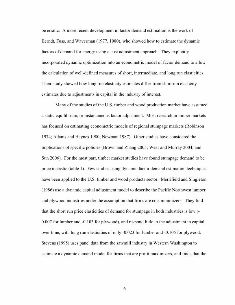
be erratic. A more recent development in factor demand estimation is the work of

Berndt, Fuss, and Waverman (1977, 1980), who showed how to estimate the dynamic

factors of demand for energy using a cost adjustment approach. They explicitly

incorporated dynamic optimization into an econometric model of factor demand to allow

the calculation of well-defined measures of short, intermediate, and long run elasticities.

Their study showed how long run elasticity estimates differ from short run elasticity

estimates due to adjustments in capital in the industry of interest.

Many of the studies of the U.S. timber and wood production market have assumed

a static equilibrium, or instantaneous factor adjustment. Most research in timber markets

has focused on estimating econometric models of regional stumpage markets (Robinson

1974; Adams and Haynes 1980; Newman 1987). Other studies have considered the

implications of specific policies (Brown and Zhang 2005; Wear and Murray 2004; and

Sun 2006). For the most part, timber market studies have found stumpage demand to be

price inelastic (table 1). Few studies using dynamic factor demand estimation techniques

have been applied to the U.S. timber and wood products sector. Merrifield and Singleton

(1986) use a dynamic capital adjustment model to describe the Pacific Northwest lumber

and plywood industries under the assumption that firms are cost minimizers. They find

that the short run price elasticities of demand for stumpage in both industries is low (-

0.007 for lumber and -0.103 for plywood), and respond little to the adjustment in capital

over time, with long run elasticities of only -0.023 for lumber and -0.105 for plywood.

Stevens (1995) uses panel data from the sawmill industry in Western Washington to

estimate a dynamic demand model for firms that are profit maximizers, and finds that the

6

elasticity of demand for sawlogs increases from -0.183 in the short run to -0.467 in the

long run.

The Lagged Adjustment Model

Following standard theory, the regional demand for softwood stumpage in a given

supply region is derived from the production of final goods, and can be specified using

the framework of production theory. For region i, Qit is the aggregate output produced by

all mills in the region i, where ),,( itititit KLSfQ = . The function f(·) is a fixed-factor

production function with inputs of stumpage (Sit), labor (Lit), and capital (Kit) used by

firms in period t. For simplicity, we assume that each region has a single, perfectly

competitive market, so that each mill faces the same input costs. The region’s aggregate

profit function is defined as:

(1) ititititititititrwpit KrLwSpQPititit

−−−= *

,,maxπ

where Pit is the regional product price, Q*it is the optimal amount of output for the end

product, and pit,, wit and rit are the respective input costs of stumpage, labor, and capital.

Applying Hotelling’s lemma, region i’s derived demand for stumpage is a function of the

demand for its output and the prices of all factors of production:

(2) ),,,( ititititDit PrwpfS =

where SDit is the stumpage demand in region i at time t.

To measure how firms are adjusting their production process over time, a one

period lag for the quantity of stumpage demanded (SDit-1) is added to the econometric

model that empirically estimates the regional derived demand functions. This

7

formulation is commonly referred to as the lagged adjustment model first derived by

Koyck (1954) and is consistent with the model suggested by Houthakker and Taylor

(1970), who show that the optimal amount of the consumption good (St*) is specified as a

function of its price (pt) and other variables (Zt) along with a disturbance term (εt), such

that the demand equation is:

(3) ∑=

+++=n

jtjtjt

Dt ZapaaS

210 ε

Equation (3) can then be put in an operational form that only contains observable

variables such that an adjustment process relating actual and desired input is observed, as

expressed in the following equation:

(4) 10)( 1*

1 ≤<−+= −− γγ for S SSS Dt

DDt

Dt

This indicates that in the current period, t, the firm will only adjust a part of the way from

the initial condition (St-1) to the desired condition (St*) in response to a change in input

prices. The closer that γ is to unity, the faster the adjustment process. Combining (3) and

(4), we get:

(5) ∑=

− ++−++=n

jtjtj

Dtt

Dt ZaSpaaS

2110 )1( εγγγγ

Incorporating our knowledge about the regional demand for stumpage, we can then

formulate regional derived demand curves, where pt is the input price for stumpage and

Zjt are other factors of derived demand, specifically capital, wage, and the price of

lumber. The parameters estimated in equation (5) can then be used to determine short-

run and long run elasticities, where a1γ is the short run response and a1γ/[1-(1- γ)] is the

long run response to a change in price.

8

Empirical Lagged Adjustment Model

The lagged adjustment model is estimated empirically for three major timber

supply regions that are distinguished by their final end products, tree species, and owner

composition. The supply and demand system for two Pacific Northwest regions, divided

between east and west by the Cascade Mountains, are both dominated by the sawmill

industry, yet differ in species and composition. The model for the South includes supply

and demand equations for both the sawmill and the pulp and paper industries, as they

each contribute to a large portion of the region’s timber sector.

Equation (5) is the industry-specific demand function, which is defined above.

The supply-side in stumpage markets is individual landowners, including both private

and governmental sources, who have production functions that depend on the biological

growth and other factors of production. Suppliers require labor, and capital stock

(standing inventory) to produce their desired amount of output, which is in turn

demanded by the mills in order to produce their final good. For the two Pacific

Northwest regions (PNWW and PNWE), we also include a dummy variable (D89) equal

to 1 for the years greater or equal to 1989 and 0 otherwise, as it acts as a fixed effect for

the supply shift caused by federal timber restrictions in the 1990s. In the case of the

South, where federally owned forests supply little timber, the price of sawnwood or

pulpwood stumpage is included to test for a potential substitution effect. The aggregate

supply function for all forest owners in a region is expressed as:

(6) ),,,( fit

fit

fit

sit

Sit YkwpfS =

9

where SSit is the total amount of stumpage demanded in a region i at time t, is the

hourly wage of a logger, is the standing merchantable inventory (million ft

fitw

fitk 3) and Yit is

the region-specific supply shifter that is discussed above. Merchantable inventory is the

inventory in age classes nearing or above the optimal rotation period.

The regional derived demand equations for the Pacific Northwest (ignoring the

pulp markets) are estimated using a demand and supply system. The demand equation

uses the factors derived in equation (5). The supply equation uses the variables defined

in equation (6) but does not include a lagged dependent variable because capital on the

supply side, merchantable forest stock, is determined over a substantially longer time

period. This system is defined as:

(7) i = PNWW, PNWE it

Dit

sit

sit

sit

sit

Dit

ititf

itmerchf

itsit

Sit

vSkwPpS

DwkpS

++++++=

+++++=

−1543210

43,

210

,

89

ββββββ

εααααα

where sitp is the volume-weighted average real price for stumpage per thousand board feet

(MBF), is a the real regional price of lumber ($/MBF),sitP s

itw is the real regional hourly

wage rate for sawmill workers, and sitk is amount of capital stock in billions of dollars.

On the supply side, is the amount of merchantable forest stock (million ftmerchfitk , 3) for the

region, and fitw is the real hourly wage rate of loggers. All prices and input costs are

deflated to 1982 dollars to be consistent with estimates from the previous literature. The

respective error terms for the supply and demand equations are εit and vit. The market

clearing condition is that quantity supplied (SSit) equals quantity demanded (SD

it), and is

measured in million cubic feet.

For the South, both the sawnwood and pulpwood markets are considered:

10

(8)

pSt

PulpDSt

pSt

pSt

pSt

pSt

PulpDSt

pSt

sSt

fSt

totfSt

pSt

PulpSSt

sSt

SawDSt

sSt

sSt

sSt

sSt

SawDSt

sSt

pSt

fSt

merchfSt

sSt

SawSSt

vSkwPpS

pwkpS

vSkwPpS

pwkpS

++++++=

+++++=

++++++=

+++++=

−

−

1543210

43,

210

1543210

43,

210

,

,

ϕϕϕϕϕϕ

εδδδδδ

ββββββ

εααααα

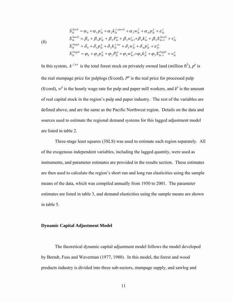
In this system, is the total forest stock on privately owned land (million fttotfk , 3), pp is

the real stumpage price for pulplogs ($/cord), PP

p is the real price for processed pulp

($/cord), wp is the hourly wage rate for pulp and paper mill workers, and kp is the amount

of real capital stock in the region’s pulp and paper industry. The rest of the variables are

defined above, and are the same as the Pacific Northwest region. Details on the data and

sources used to estimate the regional demand systems for this lagged adjustment model

are listed in table 2.

Three-stage least squares (3SLS) was used to estimate each region separately. All

of the exogenous independent variables, including the lagged quantity, were used as

instruments, and parameter estimates are provided in the results section. These estimates

are then used to calculate the region’s short run and long run elasticities using the sample

means of the data, which was compiled annually from 1950 to 2001. The parameter

estimates are listed in table 3, and demand elasticities using the sample means are shown

in table 5.

Dynamic Capital Adjustment Model

The theoretical dynamic capital adjustment model follows the model developed

by Berndt, Fuss and Waverman (1977, 1980). In this model, the forest and wood

products industry is divided into three sub-sectors, stumpage supply, and sawlog and

11

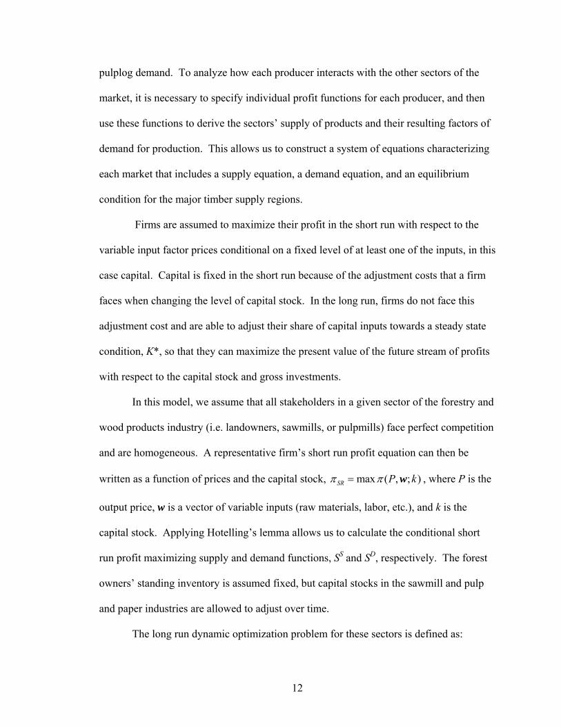
pulplog demand. To analyze how each producer interacts with the other sectors of the

market, it is necessary to specify individual profit functions for each producer, and then

use these functions to derive the sectors’ supply of products and their resulting factors of

demand for production. This allows us to construct a system of equations characterizing

each market that includes a supply equation, a demand equation, and an equilibrium

condition for the major timber supply regions.

Firms are assumed to maximize their profit in the short run with respect to the

variable input factor prices conditional on a fixed level of at least one of the inputs, in this

case capital. Capital is fixed in the short run because of the adjustment costs that a firm

faces when changing the level of capital stock. In the long run, firms do not face this

adjustment cost and are able to adjust their share of capital inputs towards a steady state

condition, K*, so that they can maximize the present value of the future stream of profits

with respect to the capital stock and gross investments.

In this model, we assume that all stakeholders in a given sector of the forestry and

wood products industry (i.e. landowners, sawmills, or pulpmills) face perfect competition

and are homogeneous. A representative firm’s short run profit equation can then be

written as a function of prices and the capital stock, max ( , ; )SR P kπ π= w , where P is the

output price, w is a vector of variable inputs (raw materials, labor, etc.), and k is the

capital stock. Applying Hotelling’s lemma allows us to calculate the conditional short

run profit maximizing supply and demand functions, SS and SD, respectively. The forest

owners’ standing inventory is assumed fixed, but capital stocks in the sawmill and pulp

and paper industries are allowed to adjust over time.

The long run dynamic optimization problem for these sectors is defined as:

12

(9) 0

max [ ( , ; ) ( ) ( )] rtP k u r k c k e dπ δ∞ •

−− + −∫ w t

where π(• ) is the profit function, u is the asset price of capital that is a function of the

discount rate, r, and the depreciation rate, δ; and ( )c k•

is the adjustment cost of capital,

which is a function of investment, or the change in capital, k•

. Using Euler’s equation of

the calculus of variation, the first-order condition of (9) for the quasi-fixed input is:

(10) π δ( )kk k k

u r rc c k• • •

••

= + + −

where πk is the first derivative of the profit function with respect to k and is the

derivative of the net capital investment with respect to time.

k••

In the long run, we assume that the capital stock fully adjusts to its optimal

steady-state level of input, k*. In this case, the annual investment ( ) and change in

investment ( ) will be equal to zero. If we also assume that adjustment costs are zero

when no investment occurs, the first order condition becomes:

k•

k••

(11) *( *, 0) ( )k k k u rπ δ•

= = +

where *kπ is the first derivative of the profit function with respect to k and k* is the

optimal level of capital stock. Equation (11) can also be interpreted as the well-known

static condition where the marginal return to capital is equal to the user cost of capital.

The demand function for the capital good can then be formalized by linearly

approximating equation (11) around the long run optimal capital stock, k*, in a manner

first presented by Lucas (1967). This method obtains a second order differential equation

that can be solved for its stable root, λ, resulting in the following equation:

13

(12) ( * )k k kλ•

= −

where λ = is a stable root is between zero and one, where

zero implies no adjustment and one implies full adjustment in that given time period

(Treadway 1971; 1974). Because discrete annual changes will be used to determine

empirical estimates, it is more convenient to rewrite equation (12) using discrete time

subscripts such that the demand equation for capital is:

21/ 2{ ( 4 / ) }kk

kkr r cπ • •− − − 1/ 2

tk(13) *1 (1 )tk kλ λ+ = + −

Equation (13) is the foundation of our capital adjustment equation, where λ is a parameter

directly estimated in the empirical dynamic factor demand system. Equation (13) and the

specified supply and demand equations can be used to empirically estimate the dynamic

factors of demand and resulting short, intermediate, and long run elasticities for the two

production sectors of the wood products industry.

Empirical Dynamic Capital Adjustment Model

Specified functional forms of the profit and capital adjustment cost equations are

necessary to empirically estimate the factor demands and resulting elasticities. Quadratic

functions are chosen as approximations of the true profit functions because of their

flexible functional form. For the empirical specification, superscripts i = f, s, and p are

used to distinguish between the three sectors: forest owners, sawmills, and the pulp and

paper industry, respectively. Capital inputs are identified by ki and considered to be the

only quasi-fixed inputs in the demand system, and w indicates variable inputs. Time

14

indexation is denoted by t, and is only used to distinguish between lead and lag variables.

For the sawmill and pulp and paper industry, the respective profit functions are:

(14)

lp,i wwwkwkkZ

kZwZZPkPwPP

ls,i wwwkwkkZ

kZwZZPkPwPP

i j

pj

piij

i

pii

pkk

i

pi

pki

pk

pZZ

ppZk

i

pi

pzi

pz

pPP

ppPk

i

pi

pPi

pP

p

i j

sj

siij

i

sii

skk

i

si

ski

sk

sZZ

ssZk

i

si

szi

sz

sPP

ssPk

i

si

sPi

sP

s

=++++++

+++++++=

=++++++

+++++++=

∑∑∑∑

∑∑

∑∑∑∑

∑∑

ϕϕϕϕϕϕ

ϕϕϕϕϕϕϕϕπ

ββββββ

ββββββββπ

5.0)(5.0)(5.0

)(5.0

5.0)(5.0)(5.0

)(5.0

22

20

22

20

where subscripts i = s,p,l denote the inputs of sawlogs, pulpwood, and labor, respectively,

PP

s indicates the market price for lumber, PpP

is the final product price for pulp, and Zi is an

exogenous shifter specific to a region’s supply or demand equation.

The aggregate supply function for forest owners in a given region is the same as

equation (6). The regional derived demand equations for stumpage are determined by

applying Hotelling’s lemma to equation (14), such that the supply and demand system is:

(15)

pp

pp

plpl

pppp

ppPp

Dp

fpz

fpk

flpl

ppppp

Sp

ssz

ssk

slsl

ssss

ssPs

Ds

fsz

fsk

flsl

sssss

Ss

ZkwwPS

ZkwwS

ZkwwPS

ZkwwS

ϕϕϕϕϕϕ

δδδδδ

ββββββ

ααααα

+++++=

++++=

+++++=

++++=

where is the sawmills’ demand for sawlogs, is the pulp and paper industry’s

demand for pulplogs, and and are the forest landowners respective annual supply

of sawlogs and pulplogs. Using equation (11), where the marginal return to capital is

equal to the user cost of capital

DsS D

pS

SsS S

pS

1, the long run optimal capital stock (k*) can be derived

from (14):

1 For this model, the user cost of capital is calculated as a function of the investment producer price index (ppiinv), the general ppi (ppitot), the interest rate (r), and a constant depreciation rate (δ), such that:

( ), ,ippii ikU r it ppitotal

δ= + s p=

15

(16) [ ]

[ ]plkl

ppkp

pkPk

p

kk

p

slkl

ssks

skPk

s

kk

s

wwPruk

wwPruk

ϕϕϕϕδϕ

ββββδβ

−−−−+=

−−−−+=

)(1

)(1

*

*

Substituting ks* and kp* into equation (13) forms the demand function for capital at the

end of period t for the sawmill and pulp and paper industries:

(17) [ ]

[ ] pt

pplkl

ppkp

pkPk

p

kk

pp

t

st

sslkl

ssks

skPk

s

kk

sst

kwwPruk

kwwPruk

)1()(

)1()(

1

1

λϕϕϕϕδϕλ

λββββδβλ

−+−−−−+=

−+−−−−+=

+

+

Combining equations (15) and (17), we now have a complete system of equations that

allows us to derive the responses in supply and demand to price changes in the short,

intermediate, and long run. As in the case of the lagged adjustment model, the system of

equations for the two Pacific Northwest regions only include the sawtimber industry,

while the South accounts for both sawlog and pulplog markets.

To also be consistent with the lagged adjustment model, region-specific

exogenous supply and demand variables were included in the system of equations.

Exogenous variables in the regional supply equations were the same as the lagged

adjustment model. Real gross domestic product per capita (GDP, in 1982$) is included

in the demand equations to test for any potential income or growth effects on regional

demand. A detailed explanation of the data and the sources where each regional statistic

was obtained for 1950-2001 is listed in table 2. All data was listed at the regional level

with the exception of capital stock, which was disaggregated by multiplying the

proportion of a region’s production relative to national production by the national

measure of capital stock. The annual changes in estimated regional capital stock values

16

were then verified using regional annual investment data that is still published on an

annual basis (U.S. Bureau of Labor Statistics 2005). Regional parameter estimates are

shown in table 4.

The short run demand responses can be interpreted simply by the parameter

estimates for α, δ, β and φ. Because this is a linear demand function, short run elasticity

is simply dS/dp( psw / S ), where p

sw is average price, and S is average quantity . The

intermediate run (IR) elasticity for stumpage price in the sawmill sector is then calculated

as follows:

(18) Sw

wS p

ssn

i

is

kk

ksskssp

s

IRDs

⎭⎬⎫

⎩⎨⎧

−+−=∂∂ ∑

=

λλβββ

β0

,

)1(

where λs is the capital adjustment parameter for sawmills and i = 1…n are the number of

years in the intermediate adjustment period (usually 2 or more years). LR elasticities are

calculated when λs is set equal to one, as this is when the long run demand for capital is

equal to the optimal capital stock.

The endogenous variables on the right hand side of the equations require using an

instrumental variable method to estimate the parameters. The endogenous variables in

the system are stumpage price, stumpage quantity, and capital stock. The rest of the

variables in the system are used as the instrument variables. In this case, the non-linear

three-stage least squares (NL3SLS) method is preferred over the seemingly unrelated

regression (SUR) method for estimating the model, as it is a consistent estimator when

the first difference of the capital stock and the error term are not independent (Greene

2003). This dependency condition is confirmed using a Hausman (1978) test.

17

Results

The results of the lagged adjustment model are shown in table 3. The negative

sign for the PNW-Westside sawlog stumpage price meets economic theory of a

downward sloping demand curve, and the positive signs on the other inputs suggest that

labor and capital are substitutes for stumpage as factors of the production process. The

large value for the lagged quantity parameter (0.66) indicates relatively slow adjustment.

The positive signs for stumpage price and inventory both match the theory that as prices

and inventories increase, so does supply. A large estimate for D89 (-820.4) accounts for

the large shift in supply due to harvest restrictions and other changes in the industry.

Results for the PNW-Eastside demand equation are all significant at the 90

percent confidence level with the exception for the price of lumber and the constant.

Stumpage price is negative and significant. The signs on the other inputs show that labor

and capital are both substitutes for stumpage in the production of sawnwood. Firms are

also slow to adjust their factors of production. For the eastside’s supply equation,

stumpage price was positive, indicating an upward sloping supply curve that fits

economic theory. Again, a large estimate for D89 (-184.7) accounts for a large shift in

sawtimber supply since the late 1980s, although the absolute decline in stumpage

quantity is not as large as the westside because the region has smaller total production.

The South sawlog parameter estimates for the lagged adjustment model were all

significant at the 90 percent level. Stumpage price was negative, and the signs on the

other inputs indicate that capital and labor are substitutes for stumpage. The estimated

18

the speed of adjustment is similar to the PNW. The variables for the South’s sawlog

supply equation were all significant at the 90 percent level or better, and sawlog

stumpage price and inventory parameters were positive, indicating that the supply

function was correctly specified. The pulplog stumpage price parameter estimate that

was included in the supply function was positive and significant, revealing that sawlogs

and pulplogs are complements. Many firms sell pulpwood as a byproduct of a softwood

harvest, so that sawlogs and pulplogs are net complements in production.

The pulplog parameter estimates for the Southern regression in the lagged

adjustment model were significant at the 90 percent level, with the exception of wage.

The pulpwood stumpage price parameter was negative, and the lower value for the lagged

quantity parameter (0.52) suggests that Southern pulpwood processing mills have a faster

adjustment rate than regional sawmills. The pulplog stumpage price was positive as was

the sawlog stumpage price parameter, reaffirming that sawlogs and pulplogs are net

complements in production.

Results for Dynamic Capital Adjustment Model

The results of the dynamic capital adjustment model are shown in table 4. Most

of the parameters in the regional supply and demand equations have the same sign and

magnitudes as the lagged adjustment models, though many estimates had a reduction in

explanatory power relative to the simple model. Many of the parameter estimates for the

capital adjustment equations were also not significant. As expected, capital and labor are

found to be substitutes for stumpage in the production process. The only exception is that

19

the parameter on labor price is insignificant in the South sawlog demand model. Labor

and capital are also found to be substitutes for pulpwood stumpage in the South.

The capital adjustment parameter (λ) is positive and significant at least at the 10%

level in all regions except the PNW-East. For the PNW-West, the parameter is 0.20,

implying that capital turns over about once every 8 years in that region. The coefficient

for the PNW-East is 0.05, but insignificant, suggesting that capital takes many years to

adjust in that region, and that investments potentially lag relative to the rest of the

economy. The capital adjustment coefficient for the South’s sawtimber industry is

approximately 0.14, which is comparable to the Pacific Northwest estimates. This

indicates that eighty percent of the change to the desired level of capital stock is

accomplished over a 10 year period. The capital adjustment parameter for the South’s

pulp and paper industry is 0.33, suggesting that there is substantially faster capital

adjustment than the sawtimber processing sector, as was also determined in the lagged

adjustment model.

These results are consistent with a national dynamic demand model for major

sectors in U.S. manufacturing developed by Berndt, Fuss, and Waverman (1980). They

estimated a partial adjustment parameter of 0.12 for all wood products, and 0.42 for pulp

and paper products. The difference between sawmill and pulp and paper mills estimates

may be explained by the structure of the production process for both industries. Pulp and

paper mills tend to be larger in size and capacity, thereby allowing more possibilities to

invest not only in new machinery but also to improve upon older machines to improve

efficiency and capacity (Ince et al., 2001). Sawmills tend to be smaller in nature and are

20

often dependent on the size and species of the available timber in a given region, thereby

limiting the ability to quickly adjust to changing market conditions.

Elasticity Estimates

In general the own-price elasticity estimates suggest relatively inelastic demand

for timber in the short run, and that all regions respond similarly to a change in stumpage

price, even without observing the same structural change or species of input. For the

PNW-Westside, SR elasticity estimates are -0.18 to -0.25, which are at the high end of

earlier estimates from Merrifield and Singleton (1986) and Haynes, Connaughton, and

Adams (1981). For the PNW-Eastside, SR elasticity ranges from -0.002 to -0.08. These

suggest fairly low elasticity in the SR, but are in-line with the earlier estimates (see table

1). For the South sawtimber market, the SR own price elasticity ranges from -0.12 to -

0.20, and for the pulp market, -0.07 to -0.15. These are both lower than the results found

in Carter (1992) and Newman (1987). These earlier models of the southern timber

markets did not account for capital adjustments, as modeled here, and therefore may have

captured some long run effects in their static models, pushing up the elasticity estimates.

The LR elasticity estimates are higher in both the lagged adjustment and dynamic

factor demand models, and supports the hypothesis of Le Chatelier’s principle. The

dynamic factor demand model also provides a method to capture an intermediate run (IR)

elasticity estimate, which is assumed to be three years for all regions. For the PNW-

Westside, we find that there is little change in the elasticity estimate from the SR to the

IR. Most of the change in elasticity occurs from the IR to the LR. Similar results are

21

found for the other regions. LR elasticities for the region are in the range of -0.35 to -

0.48. While still inelastic, this suggests that factor demand becomes more elastic in the

LR. This result can help explain the relatively quick reduction in real prices in responses

to the supply shocks of the early 1990's. For example, for the PNW-Westside, a

permanent 30% reduction in supply, such as occurred in the early 1990's, would be

expected to increase prices by 120% in the first year or two. However, over a 5-10 year

period, one would expect this price increase to moderate to only an 85% increase in

prices. While still large, the smaller price effect could have important welfare

consequences. LR elasticity estimates are similar for the PNW-Eastside, indicating that

markets will react to harvest restrictions in a similar fashion.

The South’s pulpwood demand models produced very inelastic SR elasticities that

are on the low end of estimates from other pulpwood stumpage demand studies (Carter

1992; Newman 1987). No other econometric model focusing on regional U.S. pulplog

supply and demand has attempted to distinguish between SR and LR elasticities. These

results, coupled with the large capital adjustment parameter estimated for the southern

pulpwood market, indicate that the production process is relatively consistent and that

perhaps the faster turnover of capital is able to account for this.

Wage is relatively elastic in the LR for both regions in the PNW, and it can

fluctuate more in this region than in the South. Using the earlier example where harvests

in the PNW were reduced significantly in the 1990s, we would expect to see a similar

level of decline in wages in the region over the same time period, resulting in significant

losses for workers in the timber processing industry. On the contrary, an increase in

production in the South is not expected to increase wages for that region by the same

22

magnitude, even over the long run. High elasticity estimates for the South’s dynamic

capital adjustment models suggest that fluctuations in capital are expected to occur at a

greater magnitude than the region’s labor force, regardless of whether one is employed in

the pulp and paper or sawmill industry.

The SR stumpage own-price elasticities of supply for sawlogs are inelastic for all

three regions (ranges from 0.073 to 0.258). These estimates are towards the low end of

previous studies (see table 1), and suggest that landowners are not very responsive to

fluctuating prices, and perhaps harvest on a more fixed agenda than when previous

estimates were derived in the 1980s. The pulplog stumpage supply elasticities for the

South (0.487 and 0.598) were greater than the region’s sawlog estimates, revealing that

landowners who produce pulplogs respond to short-term changes in market variables

more than sawlog producers.

Welfare Effects

Welfare changes from a supply shock vary with the specification of the supply

and demand curves. An example of how differences between SR and LR elasticity

estimates can have a large impact on welfare calculations for a given reduction in

quantity is shown in figure 1. Not shown in the graph is the series of intermediate run

demand curves, which have slopes that range between the short run (DSR) and long run

(DLR) demand. The dynamic welfare change calculations assume that the demand curve

rotates from DSR to DLR while the original equilibrium point (Q*, P*) is held constant.

The time that it takes firms to adjust to the LR is determined by the dynamic capital

23

adjustment parameter (λ). Apparent in the graph is that the supply curve must shift

farther back along the DSR relative to DLR demand curve for the change in quantity to

remain constant. This leads to significantly larger changes in welfare relative to the LR

scenario, as highlighted by the light gray areas. Welfare changes calculated along the

path of demand and supply shifts fall somewhere in between the two extremes.

Forest landowners and lumber and wood producers in the Pacific Northwest all

faced significant losses over the course of the 1990s due to changes in the structure of the

region’s timber industry, while those in the South benefited from an increase in market

share. Averages of the estimated supply and demand elasticities from the dynamic

capital adjustment model were used to calculate regional changes in welfare using an

equilibrium displacement model (see, for example, Davis and Espinoza 1998; Sun and

Kinnucan 2001). Status quo (pre-harvest reduction) equilibrium prices and quantities are

assumed to be the average price and quantity for regional stumpage from 1980-1988,

when the market was relatively stable. The SR demand curve welfare change

calculations assume a constant estimated elasticity for the duration of the supply shifts

from 1989-2001 using average estimates of the two models shown in table 5. The

dynamic demand curve assumes that the elasticity of demand changes from the SR to the

LR over time using the estimated capital adjustment parameter (λ) from the dynamic

capital adjustment model, and is estimated to be at least 10 years for all three timber

supply regions. The regional supply curve is assumed to have a constant elasticity of for

all scenarios, and is also an average of the two estimates.

Changes in welfare associated with the federal timber harvest restrictions are

calculated by differencing the actual stumpage quantities from the status quo average (P*,

24

Q*), beginning in 1989. This procedure is then used to estimate the annual shifts in the

regional supply curve relative to a hypothetical case where there were no harvest

restrictions. A summary of the estimated changes in regional consumer, producer, and

total surplus for the three timber supply regions is shown in table 6. The results are listed

as a discounted sum of annual changes in stumpage supply from 1989 to 2001. The

welfare calculations represent the present value in 1989, and assume an annual discount

rate of 0.05, thus giving more weight to the supply shifts in the earlier years of

adjustment. The total change in welfare is simply a summation of the three major

softwood supply regions.

The calculations find that harvest reductions in the entire Pacific Northwest

resulted in present value total surplus losses in the two regions’ sawlog market of $1.7 to

$1.9 billion, depending on the different elasticity and dynamic adjustment assumptions.

Large losses experienced in the PNW were not offset by welfare improvements in the

South, as the total welfare change for the three major timber supply regions ranges from -

$0.7 to -$1.1 billion. Consumer losses in the PNW are 40-48% less, and producer losses

are 40-76% larger, if estimated with a dynamic demand curve instead of the standard

short run response. The relatively larger effects on producers make sense intuitively

since the less elastic side of the market will bear the greater incidence of a change in

price. For the three regions combined, the long-run, dynamic estimates suggest a 37%

smaller welfare effect than the short-run model. Thus, estimating and using highly

inelastic demand functions to measure welfare effects over a given time period could

substantially overstate the welfare effects.

25

Discussion and Conclusions

This paper estimates two derived demand systems for softwood stumpage in three

major softwood timber supply regions. This analysis uses one of the most comprehensive

datasets in timber and wood product demand estimation, spanning from 1950 to 2001.

The methodology and elasticity estimations discussed in this paper are a pivotal step

towards obtaining a sound understanding of how the derived factors of demand in timber

markets evolve and can vary over time regions, and with the specification of the model.

Estimates derived in this paper can give researchers and policy makers more insight on

how timber markets react to various shocks over time, and help produce more efficient

timber production forecasts and the resulting welfare effects.

Results indicate that there are differences between SR and LR demand elasticities

for all timber supply regions, and these estimates can vary with the structure of the model

and regional production process. As expected, the price elasticity of demand for

stumpage increases over time, thereby satisfying the Le Chatelier principle. Elasticity

estimates for other inputs also are shown to become more elastic over time, indicating

that there is flexibility between the three factors of demand (stumpage, labor, capital)

when producers have adequate time to adjust. While the capital adjustment period is

found to be a decade or more for sawtimber markets in all regions, the adjustment period

in the South’s pulpwood market appears to be a shorter 5 years. Differences in capital

adjustment paths can be explained by the size and capacity of the pulp and paper mills

that often have economies of scale and have the capabilities to upgrade existing machines

26

and improve efficiency. Using a simple static demand model ignores this adjustment

process and consequently overstates the welfare effects.

Neither the lagged adjustment model nor the two dynamic factor demand models

consistently estimated larger degrees of changes between short run and long run

elasticities. The key contribution of the dynamic model over the lagged adjustment

model is its ability to determine the time and path that capital stock adjusts by estimating

an explicit capital adjustment parameter. This has important policy implications, as some

have called for the need to evaluate how quickly capital investments in timber growing

and manufacturing may adapt to future regional changes in forest resources (Irland et al.

2001). These slow adjustment rates imply that the adoption of technology embodied in

new capital inputs will take longer in the timber processing industry relative to other

sectors of the economy. Investment-oriented policies, such as investment tax credits, are

likely to have a limited effect on growth in the industry.

Acknowledging the difference between the SR and LR own-price elasticities of

demand has important policy implications. First, many timber supply models used to

forecast changes in the market assume that a single price elasticity estimate holds for all

periods (e.g., Adams and Haynes 1996). Second, this measurement is often obtained

using sample means of an outdated econometric model that does not include the

structural change that has occurred in recent years (Brown and Zhang 2005). These

misspecifications can have significant effects, especially in the case where the model is

investigating potential long run welfare changes associated with a given shock (Sun

2006). If the demand curve is assumed to be highly inelastic (as in the case of most of

our SR estimates), then price changes will affect total welfare differently depending on

27

the elasticity of the supply curve (which we found here to be price inelastic). As shown

in this paper, however, firms adjust in the long run to a shock by changing their inputs

and production process (or even shutting down). As firms adjust their share of inputs

over time, the slope of the derived demand curve will change. Welfare measures based

solely on short run estimates of demand will overstate consumer losses and understate

producer gains. Our analysis finds that this overstatement could be significant. For the

example of the late 1980s reduction in federal timber harvests in the western U.S., using

short-run demand curves to estimate welfare effects would cause would overstate net

welfare effects by as much as $400 million in present value terms, or 37%.

28

References Adams, D., and R.W. Haynes. 1980. “The 1980 softwood timber assessment market

model: structure, projections, and policy simulations.” Forest Science Monograph 22: 1-64.

---. 1996. The 1993 Timber Assessment Market Model: Structure, Projections and Policy

Simulations. Gen. Tech. Rep. PNW-GTR-368. Portland, OR: U.S. Department of Agriculture, Forest Service, Pacific Northwest Research Station.

Adams, D., K.C. Jackson, and R.W. Haynes. 1988. Production, Consumption, and Prices

of Softwood Products in North America – Regional Time Series Data, 1950-1985. Resour. Bull. PNW-RB-151. Portland, OR: U.S. Department of Agriculture, Forest Service, Pacific Northwest Research Station.

Adams, D., R.W. Haynes, and A.J. Daigneault. 2006. Estimated Timber Harvest by U.S.

Region and Ownership, 1950-2002. Gen. Tech. Rep. PNW-GTR-659. Portland, OR: U.S. Department of Agriculture, Forest Service, Pacific Northwest Research Station.

Bartelsman, E.J., R.A. Becker, and W.B. Gray. 2000. NBER-CES Manufacturing Industry Database. Last accessed May 25, 2006: http://www.nber.org/nberces/.

Berndt, E.R., M.A. Fuss, and L. Waverman. 1980. Dynamic adjustment models of

industrial energy demand: empirical analysis for U.S. Manufacturing, 1947-1974. Electric Power Research Institute, Res Rep EA-1613, Palo Alto, CA.

---. 1977. Dynamic models of the industrial demand for energy. Electric Power Research

Institute, Res Rep EA-580, Palo Alto, CA. Berndt, E.R., and B.C. Field, eds. 1981. Modeling and Measuring Natural Resource

Substitution. Cambridge, MA: MIT Press. Bohi, D.R. 1981. Analyzing Demand Behavior: A Study of Energy Elasticites.

Baltimore, MD: Resources For the Future, by The Johns Hopkins University Press. Brown, R., and D. Zhang. 2005. “The sustainable forestry initiative’s impact on

stumpage markets in the U.S. South.” Canadian Journal of Forest Research. 35:2056-2064.

Carter, D.R. 1999. “Structural change in Southern softwood stumpage markets.” In: K.L.

Abt and R.C. Abt, eds. Proceedings of the 1998 Southern Forest Economics Workshop. Southern Research Station, USDA Forest Service, Williamsburg, VA. pp. 112-117.

29

Davis, G.C., and M.C. Espinoza. 1998. “A unified approach to sensitivity analysis in equilibrium displacement models.” American Journal of Agricultural Economics 80:868-879.

Greene, W.H. 2003. Econometric Analysis: Fifth Edition. Upper Saddle River, NJ:

Prentice Hall. Haynes, R.W. 2006. “Will markets provide sufficient incentive for sustainable forest

management?” In R.L Deal, and S.M. White, eds. Understanding Key Issues of Sustainable Wood Production in the Pacific Northwest. Gen. Tech. Rep. PNW-GTR-626. Portland, OR: U.S. Department of Agriculture, Forest Service, Pacific Northwest Research Station, pp. 13-19.

Haynes, R.W., K.P. Connaughton, and D.M. Adams. 1981. Projections of the Demand

for National Forest Stumpage, by Region, 1980-2030. USDA Forest Service Research Paper PNW-282. Portland, OR: U.S. Dept. of Agriculture, Forest Service, Pacific Northwest Forest and Range Exp. Station.

Haynes, R.W., tech, coord. 2003. An analysis of the timber situation in the United States:

1952 to 2050. Gen. Tech. Rep. PNW-GTR-560. Portland, OR: U.S. Department of Agriculture, Forest Service, Pacific Northwest Research Station.

Houthakker, H.S., and L.D. Taylor. 1970. Consumer Demand in the United States:

Analyses and Projections. Cambridge, MA: Harvard University Press. Howard, J.L. 2003. U.S. Timber Production, Trade, Consumption, and Price Statistics,

1965-2002. Res. Pap. FPL-RP-615. Madison, WI: U.S. Department of Agriculture, Forest Service, Forest Products Laboratory.

Ince, P.J., X. Li, M. Zhou, J. Buongiorno, and M.R. Reuter. 2001. United States Paper,

Paperboard, and Market Pulp Capacity Trends by Process and Location, 1970–2000. Res. Pap. FPL-RP-602. Madison, WI: U.S. Department of Agriculture, Forest Service, Forest Products Laboratory.

Irland, L.C., D.Adams, R. Alig, C. J. Betz, C. Chen, M. Hutchins, B.A. McCarl, K. Skog,

and B.L. Sohngen. 2001. “Assessing socioeconomic impacts of climate change on U.S. forests, wood-product markets, and forest recreation.” BioScience 51(9):753-764.

Koyck, L.M. 1954. Distributed Lags and Investment Analysis. Amsterdam: North-

Holland Publishing Company. Krichene, N. 2002. “World crude oil and natural gas: a demand and supply model.”

Energy Economics 24:557-576. Lucas, R. 1967. “Optimal investment policy and the flexible accelerator.” International

Economic Review 8(1):78-85.

30

Merrifield, D.E., and W.R. Singleton. 1986. “A dynamic cost and factor demand

analysis for the Pacific Northwest lumber and plywood industries.” Forest Science 32(1):220-233.

Murray, B.W., and D.N. Wear. 1998. “Federal timber restrictions and interregional

arbitrage in U.S. lumber.” Land Economics 74(1):111-128. Newman, D.H. 1987. “An econometric analysis of the southern softwood stumpage

market: 1950-1980.” Forest Science 33(4):932-945. Robinson, V.L. 1974. “An econometric model of softwood lumber and stumpage

markets, 1947-1967.” Forest Science 20:171-179. Samuelson, P.A. 1947. Foundations of Economic Analysis. Cambridge, MA: Harvard

University Press. Smith, B.W., P.D. Miles, J.S. Vissage, and S.A. Pugh. 2004. Forest Resources of the

United States, 2002: A Technical Document Supporting the USDA Forest Service 2005 Update of the RPA Assessment. Gen. Tech. Rep. GTR-NC-241. St. Paul, MN: U.S. Department of Agriculture, Forest Service, North Central Research Station.

Stevens, J.A. 1995. “Heterogeneous labor demand in the Western Washington sawmill

industry.” Forest Science 41(1): 181-193. Sun, C. 2006. Welfare effects of forestry best management practices in the United States.

Canadian Journal of Forest Research 36:1674-1683. Sun, C., and H.W. Kinnucan. 2001. “Economic impact of environmental regulations on

southern softwood stumpage markets: A reappraisal.” Southern Journal of Applied Forestry 25(3):108-115.

Treadway, A.B . 1974. “The globally optimal flexible accelerator.” Journal of Economic

Theory 7:17-39. ---. 1971. “The rational multivariate flexible accelerator.” Econometrica. 39(5): 845-855. Wear, D. W., and B.C. Murray. 2004. “Federal timber restrictions, interregional

spillovers, and the impact on US softwood markets.” Journal of Environmental Economics and Management 47:307-330.

U.S. Bureau of Labor Statistics. 2005. Website for interactive query of manufacturing

costs. Last accessed December 10, 2005: http://www.bls.gov/data/home.htm. U.S. Council of Economic Advisors. 2005. Economic Report of the President.

Washington D.C.

31

U.S. Department of Commerce, Bureau of the Census. 1950-2004. Annual Survey of

Manufacturers. Washington D.C. ---. 1950-2004. Census of Manufacturers. Washington D.C.

32

Table 1. Summary of Econometric Studies of Softwood Stumpage Demand and Supply Elasticities

Study Region Product SR Demand LR Demand SR SupplyRobinson (1974) South Softwood -0.52Adams and Haynes (1980) SC Softwood 0.39 - 0.47Adams and Haynes (1980) SE Softwood 0.30 - 0.47Haynes et al (1981) SC Softwood -0.13Haynes et al (1981) SE Softwood -0.05Adams and Haynes (1985) SC Softwood 0.17 - 0.63Adams and Haynes (1985) SE Softwood 0.17 - 1.20Daniels and Hyde (1986) N. Carolina Hard and Soft -0.03 0.27Newman (1987) South Pulpwood -0.43 0.23Newman (1987) South Sawtimber -0.57 0.55Abt (1987) South Lumber -0.25Robinson and Fey (1990) South Softwood -0.25Abt and Kelly (1991) FL and GA Softwood -0.10 0.30 - 0.40Carter (1992) Texas Pulpwood -0.41 0.28Newman and Wear (1993) SE Sawtimber 0.22 - 0.27Newman and Wear (1993) SE Pulpwood 0.33 - 0.58Adams and Haynes (1996) SC Softwood 0.06 - 0.26Adams and Haynes (1996) SE Softwood 0.16 - 0.18Carter (1999) South Sawtimber 0.15 - 0.35Carter (1999) South Pulpwood 0.17 - 0.27Polyakov et al. (2004) Alabama Pulpwood -1.72 0.35Adams and Haynes (1980) PNW-West Softwood 0.29 - 0.32Adams and Haynes (1980) PNW-East Softwood 0.19 - 0.29Haynes et al (1981) PNW-West Softwood -0.14Haynes et al (1981) PNW-East Softwood -0.17Merrifield and Haynes (1985) PNW-West Lumber -0.001Merrifield and Haynes (1985) PNW-West Plywood 0.02Merrifield and Haynes (1985) PNW-East Lumber -0.07Merrifield and Haynes (1985) PNW-East Plywood -0.85Merrifield and Singleton (1986) PNW Lumber -0.01 -0.023Merrifield and Singleton (1986) PNW Plywood -0.10 -0.105Abt (1987) West Lumber -0.20Stevens (1995) West. WA Sawtimber -0.18 -0.47 0.42 - 0.44Adams and Haynes (1996) PNW-West Softwood 0.42 - 0.44Adams and Haynes (1996) PNW-East Softwood 0.17 - 0.40SE = South East, SC = South Central, PNW = Pacific Northwest

33

Table 2. Variables Used in the Estimation of Factor Demand Models

Variables Symbol Description Source

Softwood sawlog supply/demand

Annual supply/demand of sawlogs (million ft3), 1950-2002 Adams et al. (2006), Table 6

Softwood pulpwood supply/demand

Annual supply/demand of pulpwood (million ft3), 1950-2002 Adams et al. (2006), Table 6

Price of sawlog stumpage Average annual price of sawlogs ($/MBF) Howard (2003), Table 26 Warren (2004), Table 102

Price of pulplog stumpage Average annual price of pulplogs ($/cord) Howard (2003), Table 26

Labor costs in logging industry

Wage rate of workers in logging industry ($/hour) Howard (2003), Table 3

Standing inventory Total inventory of softwood timber on regional timberland (million ft3)

Haynes (2003), Tables 34, 36, 42, 44 Smith et al. (2004), Table 30

1989 Dummy D89 Dummy equal to one if year is 1989 or later, 0 otherwise

Years of federal timber harvest restrictions in Pacific Northwest

Price of lumber Price of regional softwood lumber ($/MBF) Howard (2003), Tables 35, 36

Price of final product pulp Price of regional softwood pulp ($/cord) Howard (2003), Table 51

Labor costs in sawmill industry

Wage rate of workers in sawmill industry ($/hour) Howard (2003), Table 3

Labor costs in pulp and paper industry

Wage rate of workers in pulp and paper industry ($/hour) Howard (2003), Table 3

Capital Stock in sawmill industry

Value of sawmill machines and buildings (billion $)

U.S. Bureau of Labor Statistics (2005) Bartlesman et al. (2000)

Capital Stock in pulp and paper industry

Value of pulp and paper mill machines and buildings (billion $)

U.S. Bureau of Labor Statistics (2005) Bartlesman et al. (2000)

User cost of capital Function of the cap. invest. ppi, general ppi, dep. rate and the interest rate

U.S. Bureau of Labor Statistics (2005) Bartlesman et al. (2000)

Depreciation rate Constant depreciation of capital stock in sawmill and pulp and paper industry

Economic Report of the President (2004)

Real interest rate r Yield on AAA bonds Economic Report of the President (2004)

flw

sP

slw

plw

sk

pP

pk

,s pt tu u

δ

sS

pS

fk

ss

s wp ,

pp

p wp ,

34

Table 3. Parameter Estimates for Regional Softwood Stumpage Demand System, Lagged Adjustment Model PACIFIC NORTHWEST - WESTSIDESAWLOG SUPPLY SAWLOG DEMANDParms Variable Estimate Parms Variable Estimate

α0 Constant -1019.0 β0 Constant -214.1α1 Stump Saw Price 3.779 ** β1 Stumpage Price -2.663 ***α2 Priv. Merch. Inv. 0.027 * β2 Lumber Price 0.745 *α3 Logging Wage 148.3 *** β3 Sawmill Wage 93.40 ***α4 1989 Dummy -820.4 *** β4 Capital 81.32

β5 Lag Quantity 0.658 ***PACIFIC NORTHWEST - EASTSIDESAWLOG SUPPLY SAWLOG DEMANDParms Variable Estimate Parms Variable Estimate

α0 Constant 62.6 β0 Constant -249.2α1 Stump Saw Price 1.134 * β1 Stumpage Price -0.473 *α2 Total Merch. Inv. 0.006 β2 Lumber Price 0.329α3 Logging Wage 21.42 *** β3 Sawmill Wage 16.88 ***α4 1989 Dummy -184.7 *** β4 Capital 382.2 ***

β5 Lag Quantity 0.671 ***SOUTHSAW SUPPLY SAW DEMANDParms Variable Estimate Parms Variable Estimate

α0 Constant 598.9 ** β0 Constant -806.9 ***α1 Stump Saw Price 2.708 * β1 Stumpage Price -2.240 **α2 Priv. Merch. Inv. 0.061 *** β2 Lumber Price 5.283 ***α3 Logging Wage -213.0 *** β3 Sawmill Wage 76.92 ***α4 Stump Pulp Price 46.92 *** β4 Capital 69.11 **

β5 Lag Quantity 0.729 ***SOUTHPULP SUPPLY PULP DEMANDParms Variable Estimate Parms Variable Estimate

δ0 Constant -1461.1 *** φ0 Constant -247.2 *δ1 Stump Pulp Price 64.88 *** φ1 Stumpage Pulp Price -8.60 *δ2 Total Private Inv. 0.0268 *** φ2 Pulp Price 10.49 ***δ3 Logging Wage 5.031 φ3 Pulpmill Wage 27.82 **δ4 Stump Saw Price 1.8734 ** φ4 Capital 71.87 ***

φ5 Lag Quantity 0.519 ***estimation using 3SLS, with exogenous variables as instruments*** significant at 1% level** significant at 5% level* significant at 10% level

35

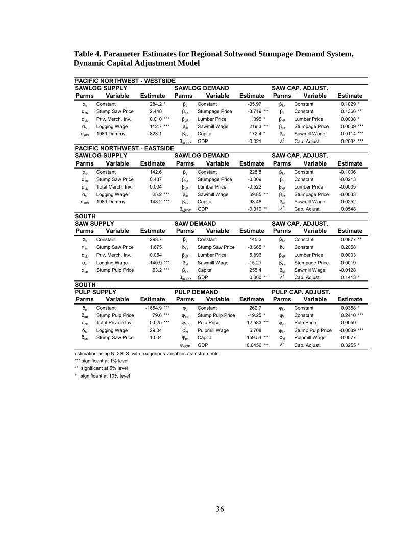
Table 4. Parameter Estimates for Regional Softwood Stumpage Demand System, Dynamic Capital Adjustment Model PACIFIC NORTHWEST - WESTSIDESAWLOG SUPPLY SAWLOG DEMAND SAW CAP. ADJUST.Parms Variable Estimate Parms Variable Estimate Parms Variable Estimate

αs Constant 284.2 * βs Constant -35.97 βkk Constant 0.1029 *αss Stump Saw Price 2.448 βss Stumpage Price -3.719 *** βk Constant 0.1366 **αsk Priv. Merch. Inv. 0.010 *** βsP Lumber Price 1.395 * βkP Lumber Price 0.0038 *αsl Logging Wage 112.7 *** βsl Sawmill Wage 219.3 *** βks Stumpage Price 0.0009 ***αs89 1989 Dummy -823.1 βsk Capital 172.4 * βkl Sawmill Wage -0.0114 ***

βsGDP GDP -0.021 λs Cap. Adjust. 0.2034 ***PACIFIC NORTHWEST - EASTSIDESAWLOG SUPPLY SAWLOG DEMAND SAW CAP. ADJUST.Parms Variable Estimate Parms Variable Estimate Parms Variable Estimate

αs Constant 142.6 βs Constant 228.8 βkk Constant -0.1006αss Stump Saw Price 0.437 βss Stumpage Price -0.009 βk Constant -0.0213αsk Total Merch. Inv. 0.004 βsP Lumber Price -0.522 βkP Lumber Price -0.0005αsl Logging Wage 25.2 *** βsl Sawmill Wage 69.85 *** βks Stumpage Price -0.0033αs89 1989 Dummy -148.2 *** βsk Capital 93.46 βkl Sawmill Wage 0.0252

βsGDP GDP -0.019 ** λs Cap. Adjust. 0.0548SOUTHSAW SUPPLY SAW DEMAND SAW CAP. ADJUST.Parms Variable Estimate Parms Variable Estimate Parms Variable Estimate

αs Constant 293.7 βs Constant 145.2 βkk Constant 0.0877 **αss Stump Saw Price 1.675 βss Stump Saw Price -3.665 * βk Constant 0.2058αsk Priv. Merch. Inv. 0.054 βsP Lumber Price 5.896 βkP Lumber Price 0.0003αsl Logging Wage -140.9 *** βsl Sawmill Wage -15.21 βks Stumpage Price -0.0019αsp Stump Pulp Price 53.2 *** βsk Capital 255.4 βkl Sawmill Wage -0.0128

βsGDP GDP 0.060 ** λs Cap. Adjust. 0.1413 *SOUTHPULP SUPPLY PULP DEMAND PULP CAP. ADJUST.Parms Variable Estimate Parms Variable Estimate Parms Variable Estimate

δp Constant -1654.9 *** φp Constant 262.7 φkk Constant 0.0358 *δpp Stump Pulp Price 79.6 *** φpp Stump Pulp Price -19.25 * φk Constant 0.2410 ***δpk Total Private Inv. 0.025 *** φpP Pulp Price 12.583 *** φkP Pulp Price 0.0050δpl Logging Wage 29.04 φpl Pulpmill Wage 6.708 φkp Stump Pulp Price -0.0089 ***δps Stump Saw Price 1.004 φpk Capital 159.54 *** φkl Pulpmill Wage -0.0077

φGDP GDP 0.0456 *** λpCap. Adjust. 0.3255 *

estimation using NL3SLS, with exogenous variables as instruments*** significant at 1% level** significant at 5% level* significant at 10% level

36

Table 5. Estimated Supply and Demand Elasticities for Three Timber Supply Regions

Lagged Dynamic Capital Adjustment Adjustment

Variable SR LR SR IRa LRPNW-W Stumpage Price -0.181 -0.483 -0.253 -0.273 -0.351Sawlog Lumber Price 0.098 0.260 0.183 0.354 1.023Demand Sawmill Wage 0.441 1.174 1.036 1.054 1.126

Capital Stock 0.093 0.246 0.000 0.829 1.907PNW-W Stump Saw Price 0.258 0.167Sawlog Logging Wage 0.724 0.550Supply Priv. Merch. Inv 0.652 0.242

PNW-E Stump Saw Price -0.079 -0.240 -0.002 -0.029 -0.506Sawlog Lumber Price 0.189 0.574 -0.299 -0.313 -0.540Demand Sawmill Wage 0.311 0.945 1.286 1.310 1.717

Capital Stock 0.415 1.263 0.000 0.439 1.010PNW-E Stump Saw Price 0.189 0.073Sawlog Logging Wage 0.409 0.228Supply Total Merch. Inv 0.368 0.480

South Stump Saw Price -0.120 -0.443 -0.197 -0.239 -0.497Sawlog Lumber Price 0.441 1.623 0.492 0.501 0.556Demand Sawmill Wage 0.219 0.805 -0.043 -0.058 -0.149

Capital Stock 0.080 0.295 0.000 1.355 3.117South Stump Saw Price 0.145 0.090Sawlog Logging Wage -0.864 -0.572Supply Priv. Merch. Inv 1.168 1.031

Stump Pulp Price 0.286 0.325South Stump Pulp Price -0.065 -0.134 -0.145 -0.242 -0.443Pulplog Pulp Price 0.241 0.887 0.289 0.453 0.794Demand Pulpmill Wage 0.176 0.647 0.042 0.113 0.259

Capital Stock 0.140 0.515 0.000 3.673 8.450South Stump Pulp Price 0.487 0.598Pulplog Logging Wage 0.025 0.145Supply Total Merch Inv 0.690 0.647

Stump Saw Price 0.124 0.066a. Intermediate run (IR) is three years for all regions and outputs

37

Table 6. Present Value of Estimated Annual Welfare Changes from Federal Harvest Restrictions, 1989-2001, Under Different Elasticity Assumptions (r=0.05)

Short Run Dynamic Difference in Estimates

million $ %PNW-W PV Δ CS (1,023)$ (617)$ -39.6%PNW-W PV Δ PS (682)$ (953)$ 39.7%PNW-W PV Δ TS (1,704)$ (1,570)$ -7.9%PNW-E PV Δ CS (226)$ (117)$ -48.3%PNW-E PV Δ PS (129)$ (227)$ 76.4%PNW-E PV Δ TS (355)$ (344)$ -3.0%South PV Δ CS 411$ 332$ -19.2%South PV Δ PS 547$ 887$ 62.0%South PV Δ TS 958$ 1,219$ 27.2%Total PV Δ CS (838)$ (402)$ -52.0%Total PV Δ PS (263)$ (293)$ 11.4%Total PV Δ TS (1,101)$ (695)$ -36.8%CS = consumer surplus, PS = producer surplus, TS = total surpluspresent value (PV) discounted to 1989, with a discount rate of 0.05

38

Figure 1. Welfare changes with short run and long run demand specifications

39