Estimating variable structure and dependence in multitask learning via gradients

ESTIMATING VARIABLE STRUCTURE IN MULTITASK LEARNING

Estimating variable structure and dependence in multitasklearningvia gradients

Justin Guinney1,2 [email protected]

Qiang Wu1,3,4 [email protected]

Sayan Mukherjee1,3,4 [email protected] Institute for Genome Sciences & Policy2 Program in Computational Biology and Bioinformatics3 Department of Statistical Science4 Department of Computer ScienceDuke UniversityDurham, NC 27708, USA

Editor: ?

Abstract

We consider the problem of hierarchical or multitask modeling in the regression context wherein addition to the regression function we seek to infer the underlying geometry and dependencebetween variables. We demonstrate how the gradient of the multiple related regression functionsover the tasks allow for dimension reduction and inference of dependencies both across tasks andspecifically for each task. We provide Tikhonov regularization algorithms for both classificationand regression that are efficient and robust for high-dimensional data, and a mechanism for incor-porating a priori knowledge of task (dis)similarity into this framework. The utility of this methodto infer geometric structure via dimension reduction, and the inference of dependencies betweenpredictive variables via graphical models is illustrated for both simulated and real data.

Keywords: multitask learning, dimension reduction, covariance estimation, inverse regression,graphical models

1. Introduction

The problem of dimension reduction in the context of regression models is of fundamental interest inthe physical and biological sciences and has a storied history (Fisher, 1922; Hotelling, 1933; Cook,2007). For much of biological and psychometric data, regression modeling needs to be extendedto respect dependencies between observations based on temporal, structural, or general subgroupstructure due to the way the data is collected. Classic examples of these regression models fallunder the purview of Bayesian hierarchical models, hierarchical models with mixed effects, and inthe context of machine learning, multitask models. These models are closely related and can berestated as independent models connected by shared hyper-priors and seek to combinesimilar datafor analysis under a single model, rather than each separately. In this paper we develop a method forsimultaneous dimension reduction and inference of dependence structure for Bayesian hierarchicalor multitask regression models. We first motivate the methodwith an important applied problem inwhole genome analysis or expression analysis in cancer genetics.

1

GUINNEY, ET AL .

Cancer like many complex traits is a heterogeneous disease requiring the accumulation of muta-tions in order to proceed through tumorigenesis, and an important problem is to predict and infer themechanism for cancer progression. For any particular cancer the genetic heterogeneity of the dis-ease is caused by two main sources: the stage or phenotypic variation of the disease and variabilityacross individuals. A regression model can be built for eachdisease state to address the heterogene-ity across the disease stage and one can select genes that arestrongly correlated with progression.The problem with this stratification approach is loss of power due to smaller sample sizes in eachseparate model and the fact that few genes or features individually may be predictive of phenotype.A natural paradigm to address this loss of power is to borrow strength across samples – multitasklearning – and borrow strength across genes – simultaneous dimension reduction and regression.We return to this application in subsection 5.4.2 where we model the progression of prostate cancer.

This same problem arises in more classical artificial intelligence applications such as digit clas-sification and text categorization since both documents andimages of digits have hierarchical struc-ture. In subsection 5.2 we illustrate this, demonstrating that inference of the distinction between a“5” and an “8” helps with discriminating a “3” from an “8.” In this case we are borrowing strengthacross the digit images and learning linear combinations ofpixels that are predictive subspaces.

The argument behind multitask learning is that pooling related samples (tasks) together in ajoint analysis can improve predictive accuracy (Evgeniou et al., 2005; Caruana, 1997; Ben-Davidand Schuller, 2003; Obozinski et al., 2006; Argyriou et al.,2006; Ando and Zhang, 2005; Jebara,2004), especially under conditions where there are few samples. Typically in this framework theidea of data similarity is traditionally considered in one of two distinct ways: sharing a similardiscriminative function, or having variables or features that tend to covary. Our objective is to modelthese two properties of the data conjointly to uncover shared structure between tasks (dependent taskvariables) as well as the task specific structure (independent task variables).

We will show that this conjoint analysis across tasks as wellas dependence structure resultsin more accurate predictive models than addressing each task individually. However, a point ofemphasis of this paper is that the inference of the predictive geometry and dependencies betweenvariables is of vital importance to interpret the results ofour models. This point is stressed inSection 5 where we use the dimension reduction and graphicalmodeling approaches we develop toinfer structure in genomic data, scientific documents, and images of digits. The key idea that willenable us to learn this structure is the simultaneous inference of both the regression (classification)function and its gradient.

2. Statistical Basis for Multitask Gradient Learning

In multitask learning we are givennt observations for each oft ∈ 1, . . . ,N tasks where the obser-

vations are drawn from a task specific joint distribution function, (Xit, Yit)nt

i=1i.i.d.∼ ρt(X,Y ). The

input variables are a subspace ofRp and the output variableYit ∈ R for regression orYit ∈ −1, 1

for classification. The total number of samples isn =∑

t nt. We will denote the observations fromthe taskt asDt andD as the set of all the observations:D = D1, . . . ,DN . The objective inmultitask modeling is to build a regression or classification function,Ft(x), for each taskt that hasa baseline termf0(x) over all tasks and a task specific correctionft(x):

Yt = Ft(x) + ε = f0(x) + ft(x) + ε, εiid∽ No(0, σ2). (1)

2


The common as well as task specific regression functions are simultaneously learned using allDobservations.

The key idea in multitask gradient learning is providing an estimate of the regression functionsf0, (ft)

Nt=1 and their gradientsf0,∇f0, (ft,∇ft)

Nt=1. The gradients provide information both

for dimension reduction as well as the inference of a conditional independence graph for the inputvariables. The central assumption in our model is that each regression function depends on a fewdimensions,d, in R

p,

Y = Ft(X) + ε = g(bT1 Xt, . . . , b

Td Xt) + ε, (2)

whereε is noise andBt = (bT1 , ..., bT

d ) is the effective dimension reduction (EDR) space.In a series of papers (Mukherjee and Zhou, 2006; Mukherjee and Wu, 2006; Mukherjee et al.,

2007; Wu et al., 2007a) a formal relation between dimension reduction and the conditional indepen-dence of predictive variables was developed. The central quantity in this relation was the gradientouter product matrixΓ, ap × p matrix with elements

Γij =

⟨

∂Ft

∂xi,∂Ft

∂xj

⟩

L2ρX

, (3)

whereρX

is the marginal distribution of the explanatory variables in taskt. Using the notationa ⊗ b = abT for a, b ∈ R

p, we can write

Γt = E(∇Ft ⊗∇Ft).

It was shown in Wu et al. (2007a) that a spectral decomposition of Γ can be used to computerelevant directions for dimension reduction. Under the semi-parametric model in equation (2) thegradient outer product matrixΓt is of rank at mostd so the relevant directions are characterized bythed eigenvectorsv1, . . . , vd associated to the nonzero eigenvalues ofΓt.

It was further shown in Wu et al. (2007a) thatΓt has a natural interpretation in terms of the co-variance of the inverse regression for each task,ΩX|Y = cov

Y[E

X(X|Y )]. Under certain conditions

the spectral decomposition ofΩX|Y can be used to compute the EDR directionsB = (b1, . . . , bd).A formal relation betweenΩX|Y andΓ can be stated for both linear as well as nonlinear regression.

For the linear case

y = βT x + ε, E ε = 0,

the following holds

Γ = σ2Y

(

1 − σ2ε

σ2Y

)2Σ−1

XΩ

X|YΣ−1

X, (4)

whereσ2Y

= var(Y ), σ2ε = var(ε), andΣ

X= cov(X) which we assume is full rank.

When the regression function is smooth and nonlinear the covariance of the inverse regressionis less intuitive but the gradient outer product matrix is still informative and can be composed as anaverage of local covariances of the inverse regression. In this case consider partitions of the inputspaceX =

⋃Ii=1 Ri such that the regression functionFt can be approximated in each partition

by a first order Taylor series expansion. Define in each partition Ri the following local quantities:the covariance of the input variablesΣi = cov(X ∈ Ri), the covariance of the inverse regressionΩi = cov(E(X ∈ Ri|Y )), the variance of the output variableσ2

i = var(Y |X ∈ Ri). Assuming

3

GUINNEY, ET AL .

that matricesΣi are full rank, the gradient outer product matrix can be computed in terms of theselocal quantities

Γ ≈I∑

i=1

ρX

(Ri)σ2i

(

1 −σ2

εi

σ2i

)2

Σ−1i Ω

iΣ−1

i . (5)

These two results suggest that learning the common gradientouter product as well as the taskspecific gradient outer products

Γ(f0) = E(∇f0 ⊗∇f0),

Γ(ft) = E(∇ft ⊗∇ft),

Γ(Ft) = E(∇Ft ⊗∇Ft),

can be used to find the common and task specific subspacesB0, (Bt)Nt=1. We will illustrate the

utility of these subspaces in Section 5.In Mukherjee et al. (2007); Wu et al. (2007a) the above conclusions were shown to extend under

weak conditions to the case where the input space is concentrated on a lower dimensional manifoldM, dM ≪ p. Details of this extension and the weak conditions under which it holds are stated inMukherjee et al. (2007); Wu et al. (2007a).

2.1 Comments

A variety of methods for simultaneous dimension reduction and regression to find directions thatare informative with respect to predicting the response variable have been proposed. These methodscan be summarized by three categories: (1) methods based on inverse regression (Li, 1991; Cookand Weisberg, 1991; Fukumizu et al., 2005; Wu et al., 2007b),(2) methods based on gradients ofthe regression function (Xia et al., 2002; Mukherjee and Zhou, 2006; Mukherjee and Wu, 2006),(3) methods based on combining local classifiers (Hastie andTibshirani, 1996; Sugiyama, 2007). Inthis paper we will build upon the approach outlined in Mukherjee and Zhou (2006); Mukherjee andWu (2006). Mathematical and statistical relations betweensome of these approaches are developedin Wu et al. (2007a).

3. Learning Multitask Gradients

3.1 Formulating the optimization problem

Given observationsD = D1, . . . ,DN over N tasks, our goal is to estimate the regression orclassification functionsf0(x), f1(x), . . . , fT (x) and gradients∇f0(x),∇f1(x), . . . ,∇fT (x).These estimates can be used to obtain the gradient outer product matrix specific to each task,Γ(ft),and the baseline gradient outer product for all tasks,Γ(f0). We will formulate the optimizationproblem to estimate functions and their gradients both for classification and regression.

For binary classification on a single task,yit ∈ −1, 1, we first define a convex loss functionφ(t) based on a link function such as the logistic link. Under thismodelFt is real-valued and maybe smooth. For example, in the case of the logistic function

φ(yFt(x)) = log(

1 + e−y Ft(x))

.

4


the classification function has a clear statistical interpretation (modelling the conditional probabilityProb(y|X) as a Bernoulli random variable)

Prob(y = ±1|x) =1

1 + e−y Ft(x).

In this case the classification function is

Ft(x) = ln

[

Prob(y = 1|x)

Prob(y = −1|x)

]

and the gradient offt exists under very mild conditions on the underlying marginal distribution. Inaddition, for a rich enough class of functionsF a Bayes optimal classifier exists

Ft = arg minFt∈F

Eρ(Xt,Yt)[φ(YtFt(Xt))].

Assume thatFt is smooth then the first order Taylor series expansion is written as

Ft(x) ≈ Ft(u) + ∇Ft(x) · (x − u), for x ≈ u. (6)

If a functionf and a vector valued function~f = (f1, . . . , fp) approximatesFt and its gradient well,then given the dataDt = (xit, yit)

nt

i=1, the expected error

E(YtFtφ(Xt)) ≈ EφDt

(f, ~f) =1

n2t

nt∑

i,j=1

w(s)i,j φ(yi(f(xj) + ~f(xi) · (xi − xj)))

is small, wherew(s)i,j is a weight function with bandwidths restricting the locality byws

i,j → 1as‖xi − xj‖ → 0. Estimates of the classification function and its gradient can be computed byminimizing the above functional with a reproducing kernel Hilbert space penalty added for regular-ization

(fDt ,~fDt) = arg min

(f, ~f)∈Hp+1

K

EφDt

(f, ~f) + λ1‖f‖2K + λ2‖~f‖2

K

,

wherefDt and ~fDt are estimates ofFt and∇Ft, respectively,‖~f‖2K =

∑pi=1 ‖fi‖

2K , andλ1, λ2

are regularization parameters. The bandwidth function imposes localization of the samples as re-quired by the Taylor expansion, while the regularization parameters provide numeric stability to theclassification and gradient functions estimates.

To extend from a single task to multiple tasks we begin with the hierarchical model in equation(1)

Ft(x) = f0(x) + ft(x),

and substitute this into equation (6)

Ft(x) ≈ f0(u) + ∇f0(x) · (x − u) + ft(u) + ∇ft(x) · (x − u), for x ≈ u. (7)

This results in an empirical error functional of the form

EφDt

(f0, ft, ~f0, ~ft) =1

n2t

nt∑

i,j=1

wi,j;tφ(

yit

(

(

f0(xjt) + ft(xjt))

+ (~f0(xjt) + ~ft(xjt)) · (xit − xjt)))

5

GUINNEY, ET AL .

where~f0 and ~ft are vector valued functions and model the gradient off0 andft respectively. Sincewe want to build a model jointly over all tasks and borrow strength across the entire data setD =D1, ...,DN we use the average empirical error over the tasks as the errorfunctional for the model

EφD

(

f0, ftNt=1 , ~f0, ~fN

t=1

)

=1

N

N∑

i=1

EφDt

(f0, ft, ~f0, ~ft).

The above functional is regularized by a RKHS penalty resulting in the following penalized errorfunctional which we minimize to obtain our classification function and gradient estimates

(

fD,0, fD,tNt=1,

~fD,0, ~fD,tNt=1

)

= arg min(ft, ~ft)T

t=0∈Hp+1

K

EφD

(

f0, ftNt=1 , ~f0, ~fN

t=1

)

+λ

2

(

‖f0‖2K + ‖~f0‖

2K

)

+µ

2N

N∑

t=1

(

‖ft‖2K + ‖~ft‖

2K

)

.

(8)

The regularization parametersµ andλ provide a priori assumptions on task similarity such thatwhen µ

λ becomes small the model puts greater emphasis on theN tasks as independent functionswhereas for a large ratio the common model dominates the optimization.

The above optimization problem can be considered as a combination of the gradient estimationideas in Mukherjee and Zhou (2006); Mukherjee and Wu (2006) with the Tikhonov regularizationformulation of multitask learning in Evgeniou and Pontil (2004). The behavior of this optimizationproblem with respect to the regularization is identical to that of Evgeniou and Pontil (2004). Notethat there are identifiably issues with the model stated in equation 7 unless we assume a priorithat∇f0⊥∇ft, i.e. the task corrected gradient is in the null space of the common gradient. Thisassumption does not effect the model fit but it does effect theinterpretation of the model.

3.2 Solving the optimization problem

A key insight in the Tikhonov regularization formulation ofmultitask learning in Evgeniou andPontil (2004) was that the multitask problem can be restatedas a single task optimization problemover all the dataD with a very particular kernel. We will couple this observation with the singletask gradient learning results in Mukherjee and Zhou (2006); Mukherjee and Wu (2006) to outlinethe classification and regression multitask gradient learning algorithms.

3.2.1 REGRESSION

We begin with regression since the resulting optimization problem is simpler. In the regressionsetting we are given observations from the regression model, yit ≈ Ft(xit), so we need only estimatethe gradients. Assuming a Gaussian noise model this resultsin the following least square taskdependent loss functional

EDt(~f0, ~ft) =

1

n2t

nt∑

i,j=1

wi,j;t

(

yit − yjt − (~f0(xjt) + ~ft(xjt)) · (xit − xjt))2

.

6


Minimizing the regularized version of the above error functional leads to the following optimizationproblem

(~fD,0, ~fD,t) = arg min(~ft)T

t=0∈Hp

K

1

N

N∑

t=1

EDt(~f0, ~ft) +

λ

2‖~f0‖

2K +

µ

2N

N∑

t=1

‖~ft‖2K

. (9)

The minimizer of this infinite dimensional optimization problem has the following finite dimen-sional representation

~f0 =∑

t

∑

i

α0,t,iK(xit, ·) ~ft =∑

i

ct,iK(xit, ·), (10)

with the coefficientsα0,t,i, ct,i ∈ Rp. This is a direct consequence of Mukherjee and Zhou (2006,

Theorem 5).Substituting the above representation into equation (9) and setting the partial derivatives to0 we

obtain the following linear system which we solve to obtain the coefficients

µct,j + Bt,j

(

N∑

s=1

ns∑

l=1

K(xls, xjt)α0,s,l +nt∑

l=1

K(xlt, xjt)ct,l

)

= Yt,j (11)

where

α0,t,i =µ

Nλct,i, (12)

Bt,j =

nt∑

i=1

1

n2t

wi,j;t(xit − xjt)(xit − xjt)T ,

Yt,j =

nt∑

i=1

1

n2t

wi,j;t(yit − yjt)(xit − xjt).

The linear system in equation (11) can be simplified based on ideas developed in Evgeniou andPontil (2004). Denote the data setD = (xi, yi)i=1,...,n as the samples arranged by task order andti as the task of the i-th sample. For example,xi = xi1 wheni ≤ n1. Denote byδst the Kroneckerdelta on tasks,δst = 1 if s = t andδst = 0 otherwise. Define the kernel

K((x, s), (x′, t)) = K(x, x′)( µ

Nλ+ δst

)

. (13)

DefineWt as thent × nt matrix with entriesWt(i, j) = 1n2

t

wi,j;t andW = diag(W1, . . . , WN ).

Let B be thenp × np matrix composed byN × N blocks where the(s, t) block is annsp × ntpsub-matrix with

Bst = 0 if s 6= t andBst = diag(Bt,1, . . . , Bt,nt) if s = t.

Let Yt = (Y Tt,1, . . . , Y

Tt,nt

)T andY = (Y T1 , . . . , Y T

N )T . We can rewrite the linear system (11) as

(

µInp + B(K ⊗ Ip))

c = Y (14)

7

GUINNEY, ET AL .

wherec = (cT1,1, . . . c

T1,n1

, cT2,1, . . . , c

T2,n2

, . . . , cTN,1, . . . , c

TN,nN

)T .Using results from Mukherjee and Zhou (2006) it can be shown that the solution of the linear

system (14) results in gradient estimates that minimize thefollowing single-task gradient learningproblem

~fD(x, t) = arg min

n∑

i,j=1

Wi,j

(

yi − yj − ~f(xi, ti) · (xi − xj))2

+ µ‖~f‖2K

,

where

~fD,0(x) + ~fD,t(x) = ~fD(x, t),

~fD,0 =µ

Nλ

N∑

t=1

~fD,t.

The linear system (14) isnp × np which whenp is large is not practically feasible. However,this linear system can be reduced to ann2 × n2 linear system using the matrix reduction argumentdeveloped for single-task gradient learning in Mukherjee and Zhou (2006).

3.2.2 CLASSIFICATION

The minimizer of the infinite dimensional optimization problem in equation (8) has the followingfinite dimensional representation

fD,0 =

N∑

t=1

nt∑

i=1

α0,t,iK(xit, ·) fD,t =

nt∑

i=1

αt,iK(xit, ·)

~fD,0 =N∑

t=1

nt∑

i=1

c0,t,iK(xit, ·) ~fD,t =

nt∑

i=1

ct,iK(xit, ·),

(15)

with coefficientsα0,t,i, αt,i ∈ R andc0,t,i, ct,i ∈ Rp. This is a direct consequence of Mukherjee and

Wu (2006, Proposition 4).Substituting the above representation into equation (8) and setting the partial derivatives to0

results in a system of equations equivalent to the following

0 =1

n2t

nt∑

i=1

wi,j;tφ′(Υi,j,t) + µαt,j

0 =1

n2t

nt∑

i=1

wi,j;tφ′(Υi,j,t)(xit − xjt) + µct,j

α0,t,i =µ

Nλαt,i

c0,t,i =µ

Nλct,i

where

Υi,j,t = yit

[

T∑

s=1

ns∑

l=1

α0,s,lK(xls, xjt) +

nt∑

l=1

αt,lK(xlt, xjt)

+(

T∑

s=1

ns∑

l=1

c0,s,lK(xls, xjt) +nt∑

l=1

ct,lK(xlt, xjt))

· (xit − xjt)]

.

8


The above system of equations is an(p + 1) × n(p + 1) system and can be solved using Newton’smethod. Note that whenp is very large this is not practical.

To address this computational problem we use the idea of reducing the multitask optimizationproblem to a single-task optimization problem with a different kernel. This allows us to use theefficient solver developed in Mukherjee and Wu (2006). Denote by D = (xi, yi)i=1,...,n thesamples rearranged in task order andti is the task associated with samplexi. Define the samekernelK as in the regression setting. LetWt be thent × nt matrix with entriesWt(i, j) = 1

n2t

wi,j;t

andW = diag(W1, . . . , WT ). Given the kernelK, weight matrixW , and dataD the followingsingle-task optimization problem can be used to compute thecoefficients for the multitask problem.The following is a direct result of the computations in Mukherjee and Wu (2006, Section 2).

Proposition 1 Consider the following single-task learning gradient problem

(gD(x, t), ~gD(x, t)) = arg ming,~g∈Hp+1

K

Eφ

D,W(g,~g) + µ‖g‖2

K+ µν‖~g‖2

K.

(16)

We havefD,0 + fD,t = gD(·, t) and ~f0 + ~ft = ~g(·, t). (17)

A result of this equivalence is that

fD,0 =µ

Nλ

N∑

t=1

fD,t and ~fD,0 =µ

Nλ

N∑

t=1

~fD,t. (18)

In Mukherjee and Wu (2006) it was shown that the single-task gradient problem could be re-duced to solving an2 × n2 nonlinear system of equations. This has been efficiently solved usingNewton’s method whenn is small.

4. Dimension reduction, task similarity, and conditional dependencies

The fundamental quantities inferred in the MTGL framework are theN + 1 gradient outer productmatricesΓ0, Γ1, ..., ΓN. These matrices and the subspaces spanned by them will be used both fordimension reduction to infer predictive structure as well as learning graphical models to infer thepredictive conditional dependencies in the data.

In Section 5 we illustrate how we can use these gradient outerproduct matrices to develop moreaccurate classifiers as well as better understand the predictive geometrical and dependence structurein the data. This analysis will require three ideas based on the gradient outer product matrices thatwe now introduce.

4.1 Dimension reduction

A primary purpose in estimating theN + 1 gradient outer product matricesΓ0, Γ1, ..., ΓN is toestimate the effective dimension reduction subspace for the common across tasks,B0, in addition tothe effective dimension reduction subspace for each task(Bt)

Nt=1. The effective dimension reduction

subspace is the span of the gradient outer productBi = span(Γi) which is computed by spectral

decomposition of the gradient outer product matrices. Given Γi the eigenvaluesλ(i)1 . . . λ

(i)p and

9

GUINNEY, ET AL .

eigenvectorsv(i)1 , . . . , v

(i)p are computed and the effective dimension reduction subspace is the

span of the eigenvectors corresponding to eigenvalues above a thresholdτ , Bi = spanv(i)k∈K

whereK = i such thatλik ≥ τ.

The immediate application of the effective dimension reduction subspaces is to project the dataonto this space and use this lower dimensional representation for classification or clustering.

4.2 Inference of task similarity

In addition to using the effective dimension subspaces for better classification accuracy, the overlapbetween these spaces provides geometric information aboutthe similarity or overlap between tasks.This can be of fundamental interest since a natural questionto ask is how related are the tasks andwhat combinations of variables characterize task similarity. We therefore construct a measure ofsubspace similarity, or overlap, as a way of measuring the relatedness of linear subspaces. Thisscore serves as a summary statistic of task similarity. We use the following measure:

Definition 2 LetΓ1 andΓ2 be twop × p symmetric (gradient outer product) matrices with entriesin R, with B1 a d-dimensional subspace ofΓ1, andB1 a f -dimensional subspace ofΓ2. Also, letv

(1)1 , . . . , v

(1)p , λ(1)

1 . . . λ(1)p andv(2)

1 . . . v(2)p , λ(2)

1 . . . λ(2)p be the eigenvectors, eigenvalues

of Γ1 andΓ2, respectively. We define the subspace overlap score (SOS) ofΓ1 andΓ2 as

SSscore1,2 =SS1→2

2+

SS2→1

2=

∑pi=1 λ

(1)i ‖P

(2)⊥ v

(1)i ‖L2

2∑p

i=1 λ(1)i

+

∑pi=1 λ

(2)i ‖P

(1)⊥ v

(2)i ‖L2

2∑p

i=1 λ(2)i

(19)

We denoteP (1)⊥ as the orthogonal projection matrix ontoB1, and determine the subspace using the

topd eigenvectors, for specifiedǫ ∈ [0, 1], such that

∑di λ

(1)i

∑pi λ

(1)i

< ǫ.

In words, the SOS is the weighted projection of one subspace onto another. Scores are in the interval[0, 1], and subspaces with complete symmetric overlap will have scores close to 1. In the case whereB1 ⊂ B2, we would expectSS1→2 ≈ 1 and it may therefore be useful to consider the two termsfrom (19) separately instead of averaged together.

4.3 Inference of graphical models and conditional dependencies

The theory of Gauss-Markov graphs (Speed and Kiiveri, 1986;Lauritzen, 1996) was developed formultivariate Gaussian densities to model conditional dependencies between variables

p(x) ∝ exp

(

−1

2xT JX + hT x

)

,

where the covariance isJ−1 and the mean isµ = J−1h. The result of the theory is that the precisionmatrix J , given byJ = Σ−1

X , provides a measurement of conditional independence. For example,Jij is said to be conditionally independent given all other variables ifJij ≈ 0. The meaning of

10


this dependence is highlighted by the partial correlation matrix RX where each elementRij is ameasure of dependence between variablesi andj conditioned on all other variablesS/ij andi 6= j

Rij =cov(xi, xj |S

/ij)√

var(xi|S/ij)√

var(xj |S/ij).

The partial correlation matrix is typically computed from the precision matrixJ

Rij = −Jij/√

JiiJjj . (20)

In the regression and classification framework inference ofthe conditional dependence betweenexplanatory variables has limited information. Much more useful would be the conditional de-pendence of the explanatory variables conditioned on variation in the response variable. Since thegradient outer product matrices provide estimates of the covariance of the explanatory variablesconditioned on variation in the response variable over all tasks and for each task, the inverses ofthese matrices

Ji = Γ−1i N

i=1,

provide evidence for the conditional dependence between explanatory variables conditioned on theresponse over all tasks and for each task. See Wu et al. (2007a) for more details on the relationbetween inference of conditional dependencies and dimension reduction.

We will use the inferred conditional dependencies to construct sparse graphs that indicate thedependence structure on simulated and biological data.

5. Experiments

We apply the multitask gradient learning algorithm (MTGL) to simulated and real data for simul-taneous classification and inference of the variable dependence structure. We explore the effect ofthe regularization parameters in modulating the bias-variance trade-off (Hastie et al., 2001) and itsimpact on predictive performance. We also compute subspaceoverlap scores to aid in our inter-pretation of the structures we infer. We restrict our analysis to the classification setting using onlyseveral tasks, although the method generalizes to any number of tasks.

5.1 Simulation

We construct two tasks containing 40 samples each (20 in class1, 20 in class-1) in a 120-dimensionalspace. We generate a data matrix for binary classification that contains features that are commonto both tasks as well as features that are specific to each task. The matrix is initialized with back-ground noise drawn fromNo(0, .2), defined as normal distributionNo(µ, σ2). We then generatesamples according to the following table, using the notation of xi as thei-th sample andxj as thej-th component:

1. task 1, class 1:xi20

i=1

xj ∼ No(2, 2), for j = 1, . . . , 10; xj ∼ No(2, .5), for j = 11, . . . , 20,

xj ∼ No(2, 2), for j = 61, . . . , 70; xj ∼ No(2, .5), for j = 71, . . . , 80

11

GUINNEY, ET AL .

2. task 1, class -1:xi40

i=21


3. task 2, class 1:xi60

i=41


xj ∼ No(2, 2), for j = 61, . . . , 70; xj ∼ No(2, .5), for j = 71, . . . , 80

4. task 2, class -1:xi80

i=61

xj ∼ No(−2, 2), for j = 91, . . . , 100; xj ∼ No(−2, .5), for j = 101, . . . , 110

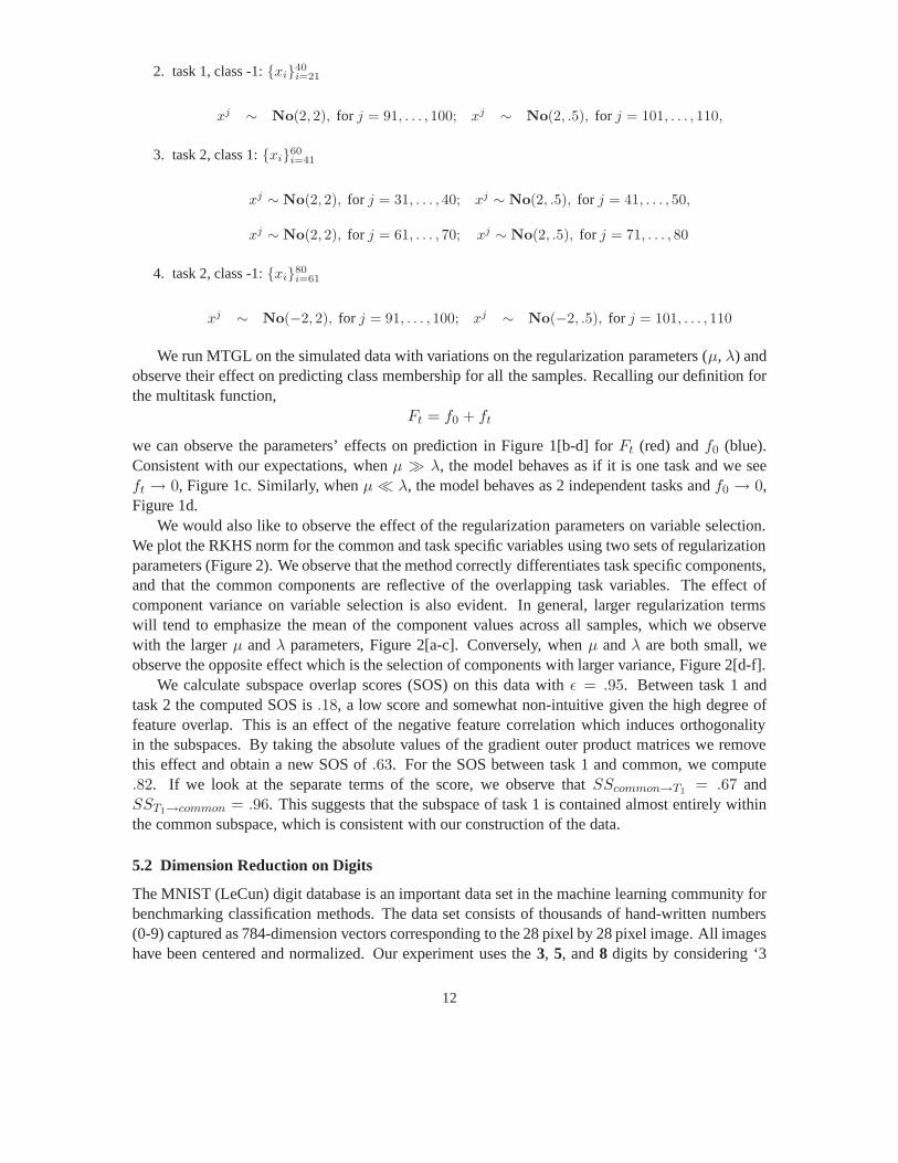
We run MTGL on the simulated data with variations on the regularization parameters (µ, λ) andobserve their effect on predicting class membership for allthe samples. Recalling our definition forthe multitask function,

Ft = f0 + ft

we can observe the parameters’ effects on prediction in Figure 1[b-d] for Ft (red) andf0 (blue).Consistent with our expectations, whenµ ≫ λ, the model behaves as if it is one task and we seeft → 0, Figure 1c. Similarly, whenµ ≪ λ, the model behaves as 2 independent tasks andf0 → 0,Figure 1d.

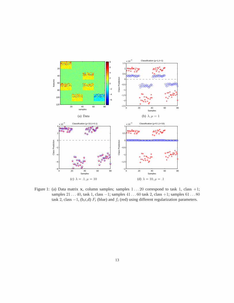
We would also like to observe the effect of the regularization parameters on variable selection.We plot the RKHS norm for the common and task specific variables using two sets of regularizationparameters (Figure 2). We observe that the method correctlydifferentiates task specific components,and that the common components are reflective of the overlapping task variables. The effect ofcomponent variance on variable selection is also evident. In general, larger regularization termswill tend to emphasize the mean of the component values across all samples, which we observewith the largerµ andλ parameters, Figure 2[a-c]. Conversely, whenµ andλ are both small, weobserve the opposite effect which is the selection of components with larger variance, Figure 2[d-f].

We calculate subspace overlap scores (SOS) on this data withǫ = .95. Between task 1 andtask 2 the computed SOS is.18, a low score and somewhat non-intuitive given the high degree offeature overlap. This is an effect of the negative feature correlation which induces orthogonalityin the subspaces. By taking the absolute values of the gradient outer product matrices we removethis effect and obtain a new SOS of.63. For the SOS between task 1 and common, we compute.82. If we look at the separate terms of the score, we observe thatSScommon→T1

= .67 andSST1→common = .96. This suggests that the subspace of task 1 is contained almost entirely withinthe common subspace, which is consistent with our construction of the data.

5.2 Dimension Reduction on Digits

The MNIST (LeCun) digit database is an important data set in the machine learning community forbenchmarking classification methods. The data set consistsof thousands of hand-written numbers(0-9) captured as 784-dimension vectors corresponding to the 28 pixel by 28 pixel image. All imageshave been centered and normalized. Our experiment uses the3, 5, and8 digits by considering ‘3

12


samples

feat

ures

20 40 60 80

20

40

60

80

100

120

−6

−4

−2

0

2

4

6

8

(a) Data

0 20 40 60 80−2.5

−2

−1.5

−1

−0.5

0

0.5

1

1.5x 10

−4 Classification (µ=1,λ=1)

Samples

Cla

ss P

redi

ctio

n

(b) λ, µ = 1

0 20 40 60 80−8

−6

−4

−2

0

2

4x 10

−4 Classification (µ=10,λ=0.1)

Samples

Cla

ss P

redi

ctio

n

(c) λ = .1, µ = 10

0 20 40 60 80−2

−1.5

−1

−0.5

0

0.5

1x 10

−3 Classification (µ=0.1,λ=10)

Samples

Cla

ss P

redi

ctio

n

(d) λ = 10, µ = .1

Figure 1: (a) Data matrixx, column samples; samples1 . . . 20 correspond to task1, class+1;samples21 . . . 40, task1, class−1; samples41 . . . 60 task2, class+1; samples61 . . . 80task2, class−1, (b,c,d)Ft (blue) andft (red) using different regularization parameters.

13

GUINNEY, ET AL .

0 20 40 60 80 100 1200

0.5

1

1.5

2

2.5

3x 10

−3

Features

Common Features (µ=1,λ=1)

(a) Common

0 20 40 60 80 100 1200

0.5

1

1.5

2

2.5

3

3.5x 10

−3

Features

RK

HS

nor

m

Task 1 Features (µ=1,λ=1)

(b) Task 1

0 20 40 60 80 100 1200

0.5

1

1.5

2

2.5

3

3.5x 10

−3

Features

RK

HS

nor

m

Task 2 Features (µ=1,λ=1)

(c) Task 2

0 20 40 60 80 100 1200

0.01

0.02

0.03

0.04

0.05

0.06

0.07

Features

RK

HS

nor

m

Common Features (µ=0.01,λ=0.01)

(d) Common

0 20 40 60 80 100 1200

0.01

0.02

0.03

0.04

0.05

0.06

0.07

0.08

Features

RK

HS

nor

m

Task 1 Features (µ=0.01,λ=0.01)

(e) Task 1

0 20 40 60 80 100 1200

0.02

0.04

0.06

0.08

0.1

0.12

Features

RK

HS

nor

m

Task 2 Features (µ=0.01,λ=0.01)

(f) Task 2

Figure 2: Variance-bias tradeoff and regularization. [a,b,c] µ, λ = 1. [d,e,f] µ, λ = .01. Highvariance features in red, low variance features in blue.

14


5 10 15 20 25

5

10

15

20

25

(a) Common

5 10 15 20 25

5

10

15

20

25

(b) Task 1: 3 vs 8

5 10 15 20 25

5

10

15

20

25

(c) Task 2: 5 vs 8

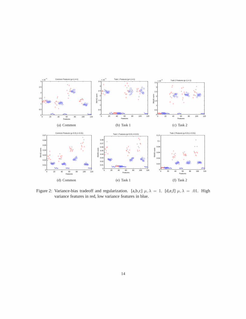
Figure 3: Digit plots of the top eigenvectors after a decomposition of the common, task 1, and task2 GOP matrices.

vs 8’ as one task, and ‘5 vs 8’ as a second task. The choice of these digits provides some helpfulintuition: the bottom half of the 3 and 5 are nearly identical, and the top halves, when taken asa composite, reproduce the top half of an 8. This therefore becomes an interesting classificationproblem. The goal of our experiment is to locate relevant subspaces within the predictive paradigm,and to compare these subspaces across tasks.

We build our data matrixX with a random selection of 50 3’s, 50 5’s, and 50 8’s, whereXi ∈R

784 andi ∈ 1, . . . , 200. We run MTGL on the data and obtain gradient outer product matricesfor the common, task 1 (3 vs 8) and task 2 (5 vs 8) models. By a spectral decomposition we canobserve the top eigenvector (corresponding to the largest eigenvalue) for each of these matrices andcompare the important components. We reshape the top eigenvector back into the 28-by-28 matrixand plot the components, see Figure 3. The dominant observable features are what we would expectgiven the canonical forms of the 3, 5, and 8 - the significant common features are located in the leftlower quadrant of the plot and correspond to the common open loop of the 3 and 5 (Figure 3a). Weobserve similar patterns in the task specific plots (Figures3b,c).

We would like to demonstrate that the subspaces obtained from the spectral decomposition arerelevant for prediction (classification). This is analogous to the well-known PCA regression whichconstructs a classifier after projection of the data onto a lower dimensional space. We use thetop l = 1, 2, 3, 4 significant eigenvectors to define a subspace for our data, and predict classmembership using the MNIST validation set (3, n=1010; 5, n=892; 8, n=974). Unlike PCA, wehave 3 subspaces in which to operate - common, task 1, and task2 - so we utilize the followingprediction strategy: we run k-nearest neighbors (kNN) in each of the subspaces separately, and usethe consensus of the largest nearest neighbor values to determine the class label. We compare ourmethod’s results with PCA regression and support vector machines (SVM, Vapnik (1998)), wherethe SVM is trained within the original component space. All regression models and SVM are trainedas ’3,5’ vs ’8’.

The above experiment is repeated 50 times and summary statistics are generated. We reportclassification accuracy as well as standard deviations, seeTable 1. Here we observe that MTGLoutperforms PCA regression considerably, reflecting the importance of utilizing response variablesfor dimension reduction. While MTGL outperforms SVM, the difference in accuracy is less sig-nificant, although it is important to note that the final regression model for MTGL has many fewervariables than the SVM model.

15

GUINNEY, ET AL .

3 5 8 Total

MTGL 94.3 (2.1) 94.0 (2.6) 82.4 (3.7) 90.2

PCA-R 85.7 (5.2) 74.4 (13.5) 72.2 (6.9) 77.6

SVM 94.0 (2.2) 91.9 (3.4) 80.6 (4.3) 88.8

Table 1: Digit classification after dimension reduction: ’3 and 5’ vs’8’. Values are percentages (standarddeviations) of prediction accuracy.

−0.1 −0.08 −0.06 −0.04 −0.02 0 0.02 0.04 0.06 0.08 0.1−0.14

−0.12

−0.1

−0.08

−0.06

−0.04

−0.02

0

0.02

0.04

0.06

1st Eigenvector

2nd

eige

nvec

tor

Earth Sciences

Astronomy

Other

(a) Common

−0.06 −0.04 −0.02 0 0.02 0.04 0.06 0.08 0.1−0.12

−0.1

−0.08

−0.06

−0.04

−0.02

0

0.02

0.04

0.06

1st eigenvector

2nd

eige

nvec

tor

Earth Sciences

Astronomy

Other

(b) Task 1 (Earth Science)

−0.12 −0.1 −0.08 −0.06 −0.04 −0.02 0 0.02 0.04 0.06−0.2

−0.15

−0.1

−0.05

0

0.05

0.1

0.15

1st eigenvector

2nd

eige

nvec

tor

Earth Sciences

Astronomy

Other

(c) Task 2 (Astronomy)

Figure 4: Earth Sciences & Astronomy vs Other. Plots depict corresponding embedding of datausing top 2 eigenvectors.

5.3 Science Documents/Words

We now consider a data set of 1047 science articles which has been previously shown to have aninterpretable hierarchical structure (Maggioni and Coifman, 2007). Each article in the documentcorpora is categorized according to one of the following 8 subjects: Anthropology, Astronomy, So-cial Sciences, Earth Sciences, Biology, Mathematics, Medicine, or Physics. We restrict our analysisto 2036 words considered most relevant over all the documents. This yields a document-word ma-trix where entry(i, j) is the frequency of wordj in documenti. We formulate a multitask learningproblem from this data by classifying Earth Sciences and Astronomy as task 1 and 2, respectively,against the remaining subjects. We randomly sample 25 documents from each of these 3 groups asinput to MTGL and learn the relevant subspaces, as was done previously. We plot the 2-dimensionalembedding of the validation data by projection on the top 2 eigenvectors (Figure 4). We observethat with just two dimensions, the categories separate well. As we would expect, the Earth Sciencecategory is harder to classify since it is more likely to haveoverlapping terms with subjects such asBiology and Anthropology.

We next use the gradient outer product matrices to extract strongly covarying components(words) by selecting large off-diagonal elements. In general, the covarying terms we observe have anatural interpretation with respect to their corresponding science categories (Table 2). The most sig-nificant covarying term for both Astronomy and Earth Sciences isearth, a term that we recognize asimmediately relevant for both subjects. Within the Astronomy task,earthco-varies with the wordsstar, galaxy, anduniverse; for Earth Science,earthstrongly co-varies withwater, lake, andocean.(From these results, we are tempted to conclude that the biggest difference between Earth and other

16


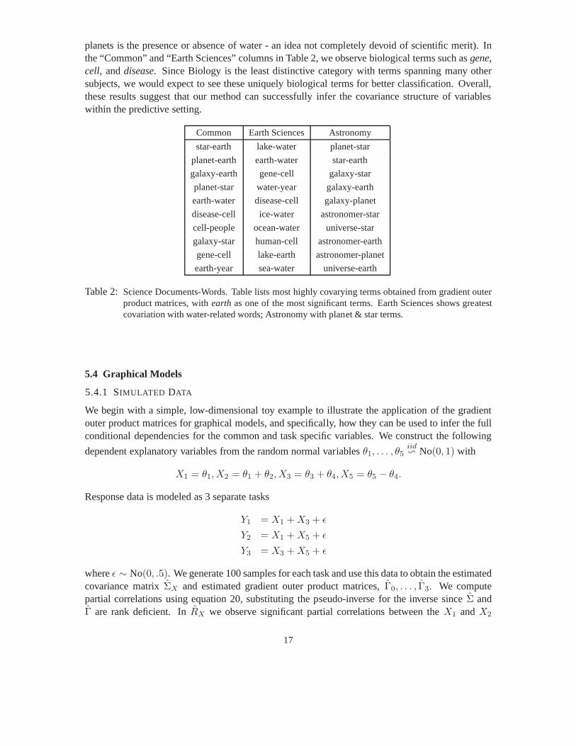
planets is the presence or absence of water - an idea not completely devoid of scientific merit). Inthe “Common” and “Earth Sciences” columns in Table 2, we observe biological terms such asgene,cell, anddisease. Since Biology is the least distinctive category with termsspanning many othersubjects, we would expect to see these uniquely biological terms for better classification. Overall,these results suggest that our method can successfully infer the covariance structure of variableswithin the predictive setting.

Common Earth Sciences Astronomy

star-earth lake-water planet-star

planet-earth earth-water star-earth

galaxy-earth gene-cell galaxy-star

planet-star water-year galaxy-earth

earth-water disease-cell galaxy-planet

disease-cell ice-water astronomer-star

cell-people ocean-water universe-star

galaxy-star human-cell astronomer-earth

gene-cell lake-earth astronomer-planet

earth-year sea-water universe-earth

Table 2: Science Documents-Words. Table lists most highly covarying terms obtained from gradient outerproduct matrices, withearthas one of the most significant terms. Earth Sciences shows greatestcovariation with water-related words; Astronomy with planet & star terms.

5.4 Graphical Models

5.4.1 SIMULATED DATA

We begin with a simple, low-dimensional toy example to illustrate the application of the gradientouter product matrices for graphical models, and specifically, how they can be used to infer the fullconditional dependencies for the common and task specific variables. We construct the following

dependent explanatory variables from the random normal variablesθ1, . . . , θ5iid∽ No(0, 1) with

X1 = θ1,X2 = θ1 + θ2,X3 = θ3 + θ4,X5 = θ5 − θ4.

Response data is modeled as 3 separate tasks

Y1 = X1 + X3 + ǫ

Y2 = X1 + X5 + ǫ

Y3 = X3 + X5 + ǫ

whereǫ ∼ No(0, .5). We generate 100 samples for each task and use this data to obtain the estimatedcovariance matrixΣX and estimated gradient outer product matrices,Γ0, . . . , Γ3. We computepartial correlations using equation 20, substituting the pseudo-inverse for the inverse sinceΣ andΓ are rank deficient. InRX we observe significant partial correlations between theX1 andX2

17

GUINNEY, ET AL .

1 2 3 4 5 6 7 8

1

2

3

4

5

6

7

8

−1

−0.8

−0.6

−0.4

−0.2

0

0.2

0.4

(a) RX

1 2 3 4 5 6 7 8

1

2

3

4

5

6

7

8

−1

−0.8

−0.6

−0.4

−0.2

0

0.2

(b) R0Γ - Common

1 2 3 4 5 6 7 8

1

2

3

4

5

6

7

8

−1

−0.8

−0.6

−0.4

−0.2

0

0.2

0.4

0.6

0.8

(c) R1Γ - Task 1

1 2 3 4 5 6 7 8

1

2

3

4

5

6

7

8

−1

−0.8

−0.6

−0.4

−0.2

0

0.2

0.4

0.6

0.8

(d) R2Γ - Task 2

1 2 3 4 5 6 7 8

1

2

3

4

5

6

7

8

−1

−0.8

−0.6

−0.4

−0.2

0

0.2

0.4

0.6

0.8

(e) R3Γ - Task 3

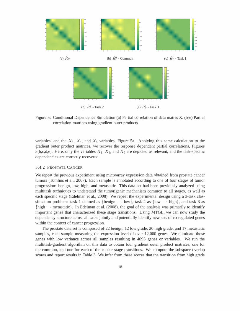
Figure 5: Conditional Dependence Simulation (a) Partial correlation of data matrix X. (b-e) Partialcorrelation matrices using gradient outer products.

variables, and theX3, X4, andX5 variables, Figure 5a. Applying this same calculation to thegradient outer product matrices, we recover the response dependent partial correlations, Figures5[b,c,d,e]. Here, only the variablesX1, X3, andX5 are depicted as relevant, and the task-specificdependencies are correctly recovered.

5.4.2 PROSTATE CANCER

We repeat the previous experiment using microarray expression data obtained from prostate cancertumors (Tomlins et al., 2007). Each sample is annotated according to one of four stages of tumorprogression: benign, low, high, and metastatic. This data set had been previously analyzed usingmultitask techniques to understand the tumorigenic mechanism common to all stages, as well aseach specific stage (Edelman et al., 2008). We repeat the experimental design using a 3-task clas-sification problem: task 1 defined asbenign → low, task 2 aslow → high, and task 3 ashigh → metastatic. In Edelman et al. (2008), the goal of the analysis was primarily to identifyimportant genes that characterized these stage transitions. Using MTGL, we can now study thedependency structure across all tasks jointly and potentially identify new sets of co-regulated geneswithin the context of cancer progression.

The prostate data set is composed of 22 benign, 12 low grade, 20 high grade, and 17 metastaticsamples, each sample measuring the expression level of over12,000 genes. We eliminate thosegenes with low variance across all samples resulting in 4095genes or variables. We run themultitask-gradient algorithm on this data to obtain four gradient outer product matrices, one forthe common, and one for each of the cancer stage transitions.We compute the subspace overlapscores and report results in Table 3. We infer from these scores that the transition from high grade

18


to metastatic represents the greatest gene expression shift, demonstrated by the largest value (.62)across the common model. The next greatest shift is seen in the transition from benign to low grade.We also observe that theben→ low andlow → high transitions are highly scored (.63) sug-gesting that the kind of genetic disregulation between these stage transitions may be one of degreeand not kind.

Common Ben→ Low Low → High High→ Met

Common – .29 .18 .62

Ben→ Low .29 – .63 .41

Low → High .18 .63 – .26

High→ Met .62 .41 .26 –

Table 3: Prostate Cancer: Subspace Overlap Scores

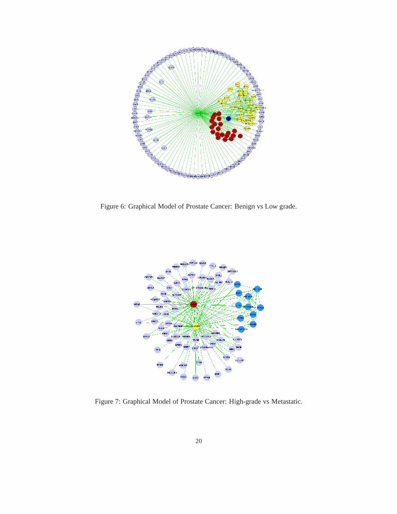
To explore the genetic dependency structure in finer detail,we construct graphical models fromthe ben → low andhigh → met gradient outer products. Since a graphical depiction of all4095 genes is too complex for visualization purposes here, we use the diagonal of the gradient outerproduct matrix to select top ranked genes. The graphs in Figures 6 & 7 recapitulate some of thebiological processes and significant genes known in prostate cancer. In the center of the first graph(ben→ low), we observe the gene MME (labeled green) connected to all other nodes in the graph,suggesting its strong global dependence. MME has been previously confirmed as strongly differen-tially expressed in aggressive prostate cancer (Tomlins etal., 2007). Also in this graph, we observetwo distinct clusters; we label theseC1 andC2 and annotate them in the graph with red and yellow,respectively. The genes in clusterC1 are not connected with each other but do all share an edge withENG (labled blue) and MME. ClusterC2, on the other hand, has many interconnections within thecluster in addition to connections with MME and ENG. ENG (Endoglin) has been previously impli-cated in vasculature development (angiogenesis), and is animportant hallmark of tumor growth. InclusterC2 we identify many well known prostate cancer genes includingAMACR, ANXA1, CD38and TFβ3.

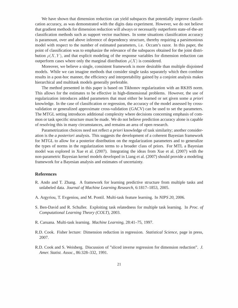
In Figure 7 we depict the gene dependency graph for thehigh → met progression. Thelabeled is dominated by two genes ABCC4 and PLA2G2A annotated in red and yellow respec-tively. ABCC4 has the pseudonym MRP (multi-drug resistant protein) and is known to have ele-vated expression in chemo-insensitive tumors, while PLA2G2A has also been identified in malig-nant prostate cancer (Jiang et al., 2002). The cluster in blue is strongly interconnected and containsseveral genes with known roles in prostatic tumor growth.

6. Discussion

We have presented a framework for dimension reduction of multivariate, multitask data in the pre-dictive setting. In addition to finding relevant subspaces,our method is capable of learning thedependency structure of variables, allowing estimation ofthe full conditional dependency matrixand the construction of graphical models. Our method is based on the simultaneous learning ofthe regression function and its gradient, formulated as a linear combination of common and taskspecific components. Assuming smooth functions over all tasks, we can use the Taylor expansionto estimate gradients.

19

GUINNEY, ET AL .

Figure 6: Graphical Model of Prostate Cancer: Benign vs Low grade.

Figure 7: Graphical Model of Prostate Cancer: High-grade vsMetastatic.

20


We have shown that dimension reduction can yield subspaces that potentially improve classifi-cation accuracy, as was demonstrated with the digits data experiment. However, we do not believethat gradient methods for dimension reduction will always or necessarily outperform state-of-the-artclassification methods such as support vector machines. In some situations classification accuracyis paramount, over and above inference of dependency structure, thereby requiring a parsimoniousmodel with respect to the number of estimated parameters, i.e. Occam’s razor. In this paper, thepoint of classification was to emphasize the relevance of thesubspaces obtained for the joint distri-bution ρ(X,Y ), and that explicit modeling of the response variables for dimension reduction canoutperform cases where only the marginal distributionρ(X) is considered.

Moreover, we believe a single, consistent framework is moredesirable than multiple disjointedmodels. While we can imagine methods that consider single tasks separately which then combineresults in a post-hoc manner, the efficiency and interpretability gained by a conjoint analysis makeshierarchical and multitask models generally preferable.

The method presented in this paper is based on Tikhonov regularization with an RKHS norm.This allows for the estimates to be effective in high-dimensional problems. However, the use ofregularization introduces added parameters that must either be learned or set given somea prioriknowledge. In the case of classification or regression, the accuracy of the model assessed by cross-validation or generalized approximate cross-validation (GACV) can be used to set the parameters.The MTGL setting introduces additional complexity where decisions concerning emphasis of com-mon or task specific structure must be made. We do not believe prediction accuracy alone is capableof resolving this in many circumstances, and remains an areaof open research.

Parametrization choices need not reflecta priori knowledge of task similarity; another consider-ation is thea posteriorianalysis. This suggests the development of a coherent Bayesian frameworkfor MTGL to allow for a posterior distribution on the regularization parameters and to generalizethe types of norms in the regularization terms to a broader class of priors. For MTL a Bayesianmodel was explored in Xue et al. (2007). Integrating the ideas from Xue et al. (2007) with thenon-parametric Bayesian kernel models developed in Liang et al. (2007) should provide a modelingframework for a Bayesian analysis and estimates of uncertainty.

References

R. Ando and T. Zhang. A framework for learning predictive structure from multiple tasks andunlabeled data.Journal of Machine Learning Research, 6:1817–1853, 2005.

A. Argyriou, T. Evgeniou, and M. Pontil. Multi-task featurelearning. InNIPS 20, 2006.

S. Ben-David and R. Schuller. Exploiting task relatedness for multiple task learning. InProc. ofComputational Learning Theory (COLT), 2003.

R. Caruana. Multi-task learning.Machine Learning, 28:41–75, 1997.

R.D. Cook. Fisher lecture: Dimension reduction in regression. Statistical Science, page in press,2007.

R.D. Cook and S. Weisberg. Discussion of ”sliced inverse regression for dimension reduction”.J.Amer. Statist. Assoc., 86:328–332, 1991.

21

GUINNEY, ET AL .

E.J. Edelman, J. Guinney, J. Chi, P.G. Febbo, and S. Mukherjee. Modeling cancer progression viapathway dependencies.PLoS Comput. Biol., 4(2), 2008.

T. Evgeniou and M. Pontil. Regularized multi-task learning. In Proc. Conference on KnowledgeDiscovery and Data Mining, 2004.

T. Evgeniou, C. Micchelli, and M. Pontil. Learning multipletasks with kernel methods.Journal ofMachine Learning Research, 6:615–637, 2005.

R.A. Fisher. On the mathematical foundations of theoretical statistics.Philosophical Transactionsof the Royal Statistical Society A, 222:309–368, 1922.

K Fukumizu, FR Bach, and MI Jordan. Dimensionality reduction in supervised learning with re-producing kernel Hilbert spaces.Journal of Machine Learning Research, 5:73–99, 2005.

T. Hastie and R. Tibshirani. Discriminant analysis by Gaussian mixtures.J. Roy.Statist. Soc. Ser. B,58(1):155–176, 1996.

T. Hastie, R. Tibshirani, and J. Friedman.The Elements of Statistical Learning. Springer, 2001.

H. Hotelling. Analysis of a complex of statistical variables in principal components.Journal ofEducational Psychology, 24:417–441, 1933.

T. Jebara. Multi-task feature and kernel selection for svms. In Proc. of ICML, 2004.

J Jiang, B Neubauer, J Graff, M Chedid, J Thomas, N Roehm, S Zhang, G Eckert, M Koch, J Eble,and L Cheng. Expression of group iia secretory phospholipase a2 is elevated in prostatic intraep-ithelial neoplasia and adenocarcinoma.Am. Jour. Pathology, 160:667–671, 2002.

S.L. Lauritzen.Graphical Models. Oxford: Clarendo Press, 1996.

Y. LeCun. Mnist database. URLhttp://yann.lecun.com/exdb/mnist.

K.C. Li. Sliced inverse regression for dimension reduction. J. Amer. Statist. Assoc., 86:316–342,1991.

F. Liang, K. Mao, S. Mukherjee, M. Liao, and M. West. Non-parametric Bayesian kernel models.2007.

M Maggioni and R Coifman. Multiscale analysis of data sets using diffusion wavelets.Proc. DataMining for Biomedical Informatics, 2007.

S. Mukherjee and Q. Wu. Estimation of gradients and coordinate covariation in classification.J.Mach. Learn. Res., 7:2481–2514, 2006.

S. Mukherjee and DX. Zhou. Learning coordinate covariancesvia gradients.J. Mach. Learn. Res.,7:519–549, 2006.

S. Mukherjee, Q. Wu, and D. Zhou. Learning gradients and feature selection on manifolds. 2007.

G. Obozinski, B. Taskar, and M. Jordan. Multi-task feature selection. Technical report, Dept. ofStatistics, University of California, Berkeley, 2006.

22


T. Speed and H. Kiiveri. Gaussian Markov distributions overfinite graphs.Ann. Statist., 14:138–150, 1986.

Masashi Sugiyama. Dimensionality reduction of multimodallabeled data by local fisher discrimi-nant analysis.J. Mach. Learn. Res., 8:1027–1061, 2007.

S.A. Tomlins, R. Mehra, D.R. Rhodes, X. Cao, L. Wang, S.M. Dhanasekaran, S. Kalyana-Sundaram, J.T. Wei, M.A. Rubin, K.J. Pienta, R.B. Shah, and A.M. Chinnaiyan. Integrativemolecular concept modeling of prostate cancer progression. Nature Genetics, 39(1):41–51, 2007.

V.N. Vapnik. Statistical Learning Theory. Wiley, New York, 1998.

Q. Wu, J. Guinney, M. Maggioni, and S. Mukherjee. Learning gradients: predictive models thatreflect geometry and dependencies. 2007a.

Q. Wu, F. Liang, and S. Mukherjee. Regularized sliced inverse regression for kernel models. Tech-nical Report 07-25, ISDS, Duke Univ., 2007b.

Y. Xia, H. Tong, W. Li, and L-X. Zhu. An adaptive estimation ofdimension reduction space.J.Roy.Statist. Soc. Ser. B, 64(3):363–410, 2002.

Y. Xue, X. Liao, L. Carin, and B Krishnapuram. Multi-task learning for classication with dirichletprocess priors.Journal of Machine Learning Research, 8:35–63, 2007.

23

Estimating variable structure and dependence in multitask learning via gradients

Documents

Transcript of Estimating variable structure and dependence in multitask learning via gradients