A comparative study of ocean thermal gradients A comparative study of ocean thermal gradients from GHRSST Level 4 SST productsfrom GHRSST Level 4 SST products

Marouan Bouali, Jorge Vazquez-Cuervo, Paulo Polito and Olga SatoMarouan Bouali, Jorge Vazquez-Cuervo, Paulo Polito and Olga Sato

2020thth GHRSST International Science Team Meeting GHRSST International Science Team MeetingESA/ESRIN, Frascati, Italy, 3-7 June 2019ESA/ESRIN, Frascati, Italy, 3-7 June 2019

Outline

Importance of fronts

Statistics vs Geometry

SST gradients from Level 4 productsFeature resolutionTemporal variability

Conclusion

Fronts in oceanography

Aqua MODIS, February 4, 2019Aqua MODIS, February 4, 2019

Landsat 8, OLI, June 3, 2018Landsat 8, OLI, June 3, 2018

Aqua MODIS, July 5, 2018Aqua MODIS, July 5, 2018Aqua MODIS, March 18, 2019Aqua MODIS, March 18, 2019

Marine ecosystem boundaries

Fisheries

Ocean 2D / 3D dynamics

Ocean-Atmosphere interaction

https://oceancolor.gsfc.nasa.gov/gallery/

Product selection for SST gradients

“What's the “best” Level 4 product for SST gradients?”

Fronts in synoptic maps Fishing spots Submarine acoustic communication

Seasonal variability Coastal Upwelling Ocean models

Long term change Impact of climate on ocean frontal activity

>10 Years

Tem

po

ral

Co

vera

ge

Daily

Fronts in synoptic mapsFronts in synoptic maps Fishing spots Submarine acoustic communication

Seasonal variability Seasonal variability Coastal Upwelling Ocean models

Long term change Long term change Impact of climate on ocean frontal activity

>10 Years

Tem

po

ral C

ove

rag

e

Daily

Can we use in situ measurements to evaluate the quality of a dataset with respect to SST gradients?

“What's the “best” Level 4 product for SST gradients?”

Statistics vs Geometry

Bias = 0.16˚CStdev = 0.5˚C

Matchup

In situ Satellite

1km

Statistics vs Geometry

Matchup

In situ Satellite

Bias = 0.16˚CStdev = 0.5˚C

Statistics vs Geometry

Matchup

In situ Satellite

Bias = 0.16˚CStdev = 0.5˚C

Statistics vs Geometry

Matchup

In situ Satellite

Same statisticsSame statisticsDifferent geometries...Different geometries...

How consistent are SST gradients from GHRSST Level 4 datasets?How consistent are SST gradients from GHRSST Level 4 datasets?

6 GHRSST Level 4 SST (2016-2018)

Canadian Meteorological Center CMC

Naval Oceanographic Office K10

Remote Sensing Systems REMSS_MW_IR

UK MetOffice OSTIA

Danish Meteorological Institute DMI

NASA/JPL Multiscale Ultrahigh Resolution MUR

All data downloaded from PODAAC and reprojected to a 0.1°Lat/Lon grid

Datasets

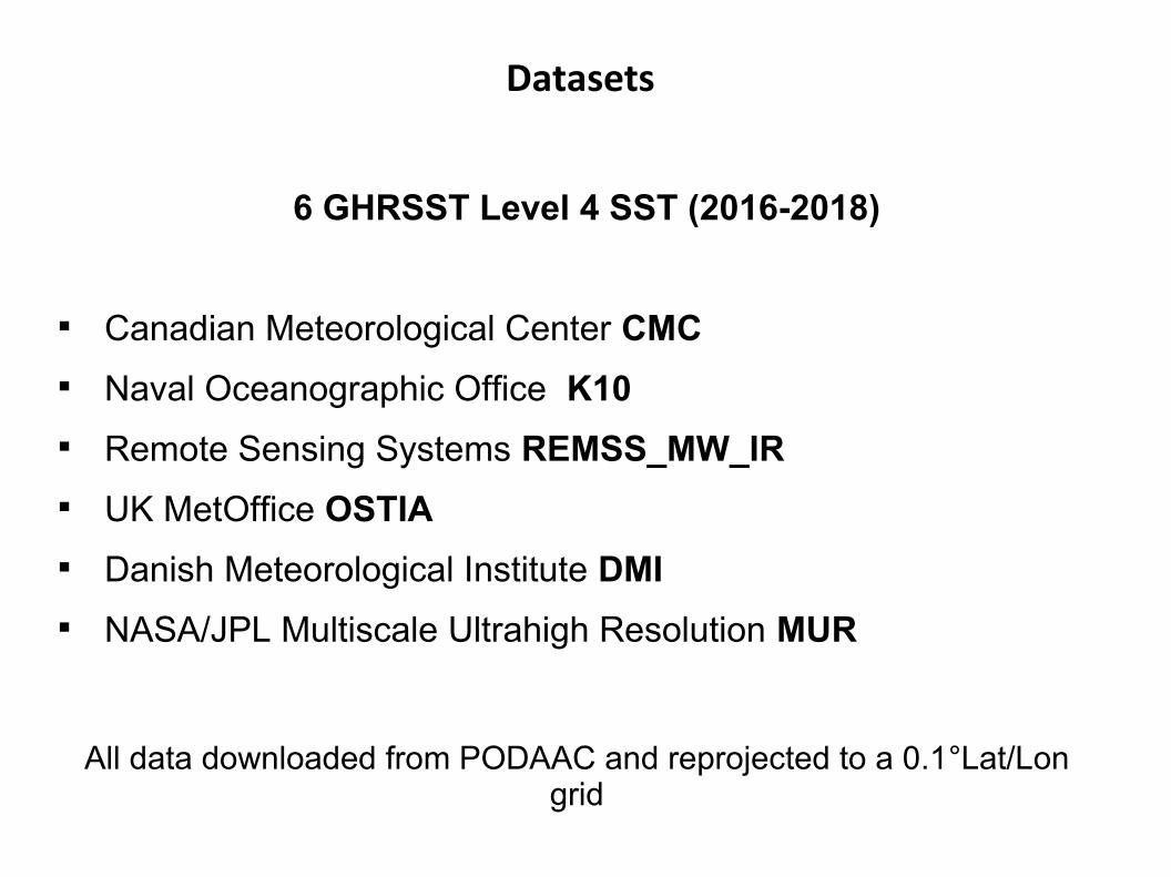
Comparison over 5 regions

Brazil-Malvinas confluence region

California Current System

Agulhas current and retroflection zone

Gulf Stream

Peruvian Upwelling System

Datasets

INFRARED MICROWAVE

In situIn situ MODISMODIS AVHRRAVHRR VIIRSVIIRS ABIABI GOESGOES SEVIRISEVIRI AMSR-EAMSR-E AMSRE-2AMSRE-2 TMITMI GMIGMI WINDSAT

CMCCMC K10K10

REMSSREMSS

OSTIAOSTIA

DMIDMI MURMUR

Datasets

Feature resolution

Aqua MODIS Dec 31 2018, Brazil-Malvinas (Level 2P, 1 km)

~300 km

CMC K10 REMSS

OSTIA DMI MUR

MODIS

Level 3U (0.1° grid)

Level 4 (0.1° grid)

Feature resolution

Bias Stdv MSE

CMC 0.32˚ 0.59˚ 0.460.46

K10 0.28˚ 0.37˚ 0.22

REMSS 0.00˚ 0.41˚ 0.17

OSTIA 0.34˚ 0.48˚ 0.35

DMI 0.29˚ 0.55˚ 0.39

MUR 0.65˚ 0.23˚ 0.470.47

SST_OBS SST_REF

err_1

err_2

Mean Squared ErrorMSE = (err_12+err_22+....)/N

Feature resolution

CMC K10 REMSS

OSTIA DMI MUR

MODIS

Bias Stdv MSE SSIM*

CMC 0.32˚ 0.59˚ 0.46 0.59

K10 0.28˚ 0.37˚ 0.22 0.79

REMSS 0.00˚ 0.41˚ 0.17 0.76

OSTIA 0.34˚ 0.48˚ 0.35 0.66

DMI 0.29˚ 0.55˚ 0.39 0.72

MUR 0.65˚ 0.23˚ 0.47 0.910.91

* Structural similarity (SSIM) indexWang, Zhou; Bovik, A.C.; Sheikh, H.R.; Simoncelli, E.P. (2004). "Image quality assessment: from error visibility to structural similarity". IEEE Transactions on Image Processing. 13 (4): 600–612Citations May 2019 > 21400

Feature resolution

SST_OBS SST_REF

CMC K10 REMSS

OSTIA DMI MUR

MODIS

Interannual variability: SSTInterannual variability: SST

Interannual variability: Interannual variability: ||▽▽SST|SST|

Histogram of |Histogram of |▽▽SST|SST|

Histogram of SST gradient magnitudes from Level 4 (Daily, Global)

Annual Cycle: Annual Cycle: ||▽▽SST|SST|

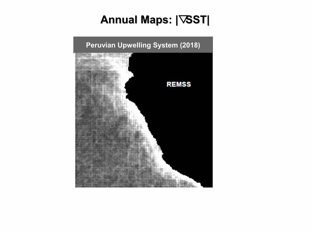
Annual Maps: Annual Maps: ||▽▽SST|SST|

Peruvian Upwelling System (2018)

CMC K10 REMSS

OSTIA DMI MUR

Annual Maps: Annual Maps: ||▽▽SST|SST|

Peruvian Upwelling System (2018)

Annual Maps: Annual Maps: ||▽▽SST|SST|

CMC K10 REMSS

OSTIA DMI MUR

Brazil-Malvinas (2018)

Annual Maps: Annual Maps: ||▽▽SST|SST|

Brazil-Malvinas (2018)

CMC

Conclusion

The magnitude of SST gradients from Level 4 products shows major differences in space and time despite consistency of SST

Differences originate from the SST analysis AND the Level 2 data ingested

Statistical metrics (Bias, Stdv, MSE) do not quantify the “geometrical quality” of SST fields (i.e., Statistical validation ≠ Geometrical validation)

Validation of SST gradients requires new methods and metrics

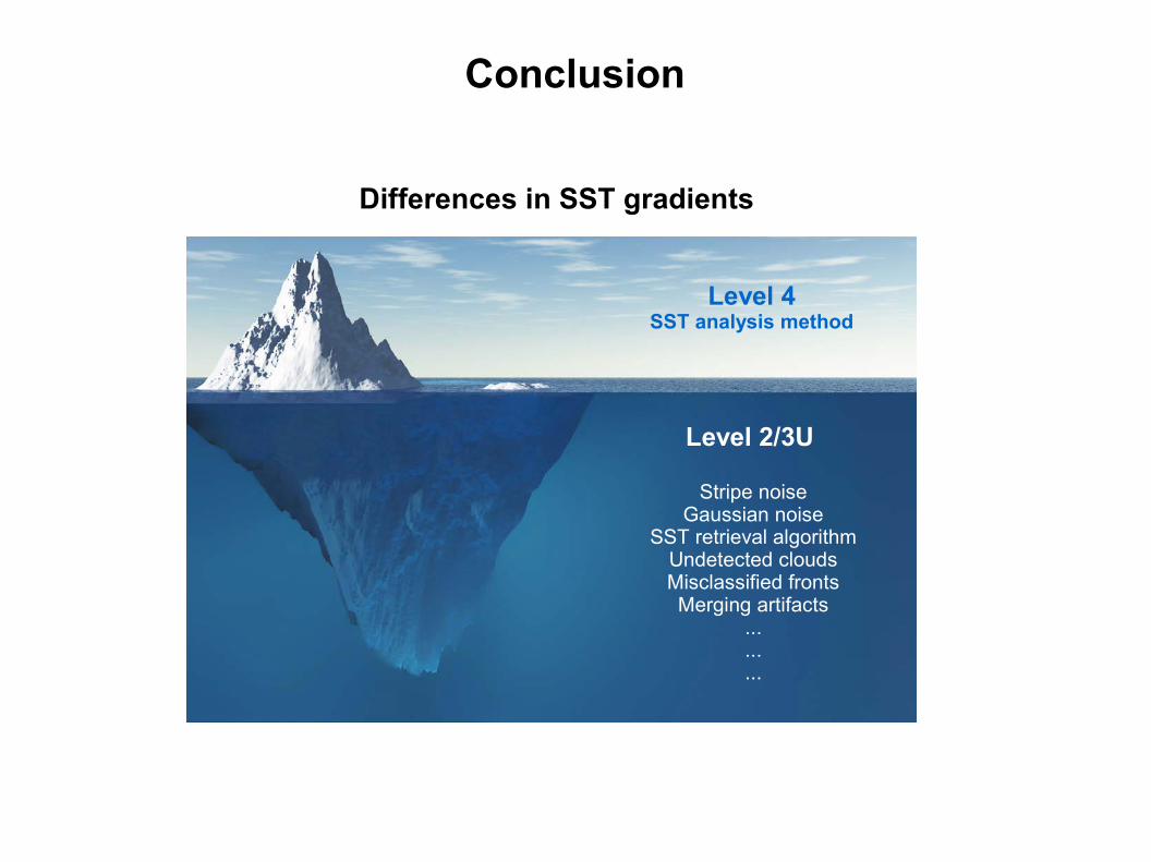
Conclusion

Differences in SST gradients

Level 4SST analysis method

Level 2/3U

Stripe noiseGaussian noise

SST retrieval algorithmUndetected cloudsMisclassified frontsMerging artifacts

...

...

...

Case study SST gradients from Level 2 MODIS

California Current System

Case study SST gradients from Level 2 MODIS

California Current System

Increasing trend of SST gradients on Terra MODIS due to continuous degradation of detectors in channels used for SST

Thank you! Questions?